Embed Size (px)
Citation preview
1
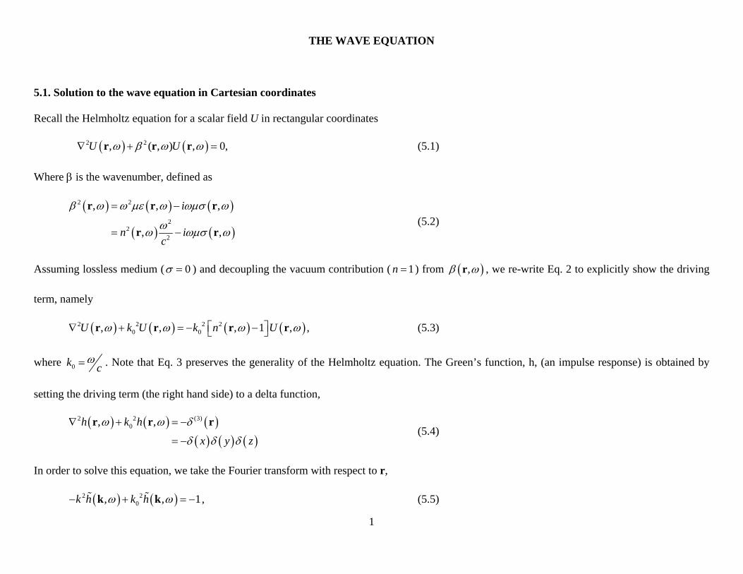
THE WAVE EQUATION
5.1. Solution to the wave equation in Cartesian coordinates
Recall the Helmholtz equation for a scalar field U in rectangular coordinates
2 2, ( , ) , 0,U U r r r (5.1)
Where is the wavenumber, defined as
2 2
22
2
, , ,
, ,
i
n ic
r r r
r r (5.2)
Assuming lossless medium ( 0 ) and decoupling the vacuum contribution ( 1n ) from , r , we re-write Eq. 2 to explicitly show the driving
term, namely
2 2 2 20 0, , , 1 , ,U k U k n U r r r r (5.3)
where 0k c . Note that Eq. 3 preserves the generality of the Helmholtz equation. The Green’s function, h, (an impulse response) is obtained by
setting the driving term (the right hand side) to a delta function,
2 2 (3)0, ,h k h
x y z
r r r (5.4)
In order to solve this equation, we take the Fourier transform with respect to r,
2 20, , 1k h k h k k , (5.5)
2
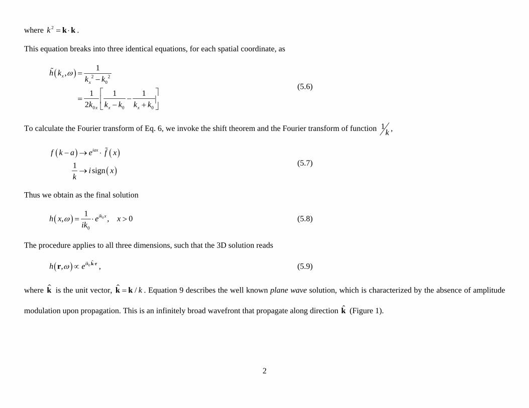
where 2k k k .
This equation breaks into three identical equations, for each spatial coordinate, as
2 20
0 0 0
1,
1 1 12
xx
x x x
h kk k
k k k k k
(5.6)
To calculate the Fourier transform of Eq. 6, we invoke the shift theorem and the Fourier transform of function 1k ,
1 sign
iaxf k a e f x
i xk
(5.7)
Thus we obtain as the final solution
0
0
1, , 0ik xh x e xik
(5.8)
The procedure applies to all three dimensions, such that the 3D solution reads
, 0ikh e k rr , (5.9)
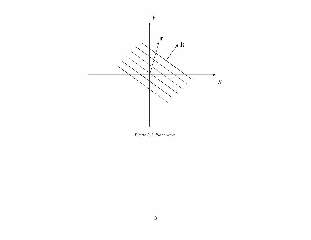
where k is the unit vector, / kk k . Equation 9 describes the well known plane wave solution, which is characterized by the absence of amplitude
modulation upon propagation. This is an infinitely broad wavefront that propagate along direction k̂ (Figure 1).
3
k
y
r
x
Figure 5-1. Plane wave.
4
5.2. Solution of the wave equation in spherical coordinates
For light propagation with spherical symmetry, such as emission from a point source in free space, the problem becomes on dimensional, with the
radial coordinate as the only variable,
(1)(3)
2
(3)
, ,
, ,
121
h U r
h U k
rr
r
k
r
r
(5.10)
Recall that the Fourier transform pair is defined in this case as
2
0
2
0
sinc
sinc
h r h k kr k dk
h k h r kr r dr
(5.11)
The Fourier properties of (3) r and 2 extend naturally to the spherically symmetric case as
(3)
2 2
1r
k
(5.12)
Thus, by Fourier transforming Eq. 4, we obtain the frequency domain solution,
2 20
1,h kk k
(5.13)
5
Not surprisingly, the frequency domain solutions for the Cartesian and spherical coordinates (Eqs. 6 and 13, respectively) look quite similar, except
that the former depends on one component of the wave vector and the latter on the modulus of the wave vector. The solution in the spatial domain
becomes
22 2
00
0 00
00
sin1,
1 1 12 2
1 .4
ikr ikr
ikr
krh r k dk
k k kr
e e dkr k k k k i
e dkir k k
(5.14)
We recognize in Eq. 15 the Fourier transform of a shifted 1k function, which we encountered earlier (Eqs. 7). Thus, evaluating this Fourier
transform, we finally obtain Green’s function for propagation from a point source,
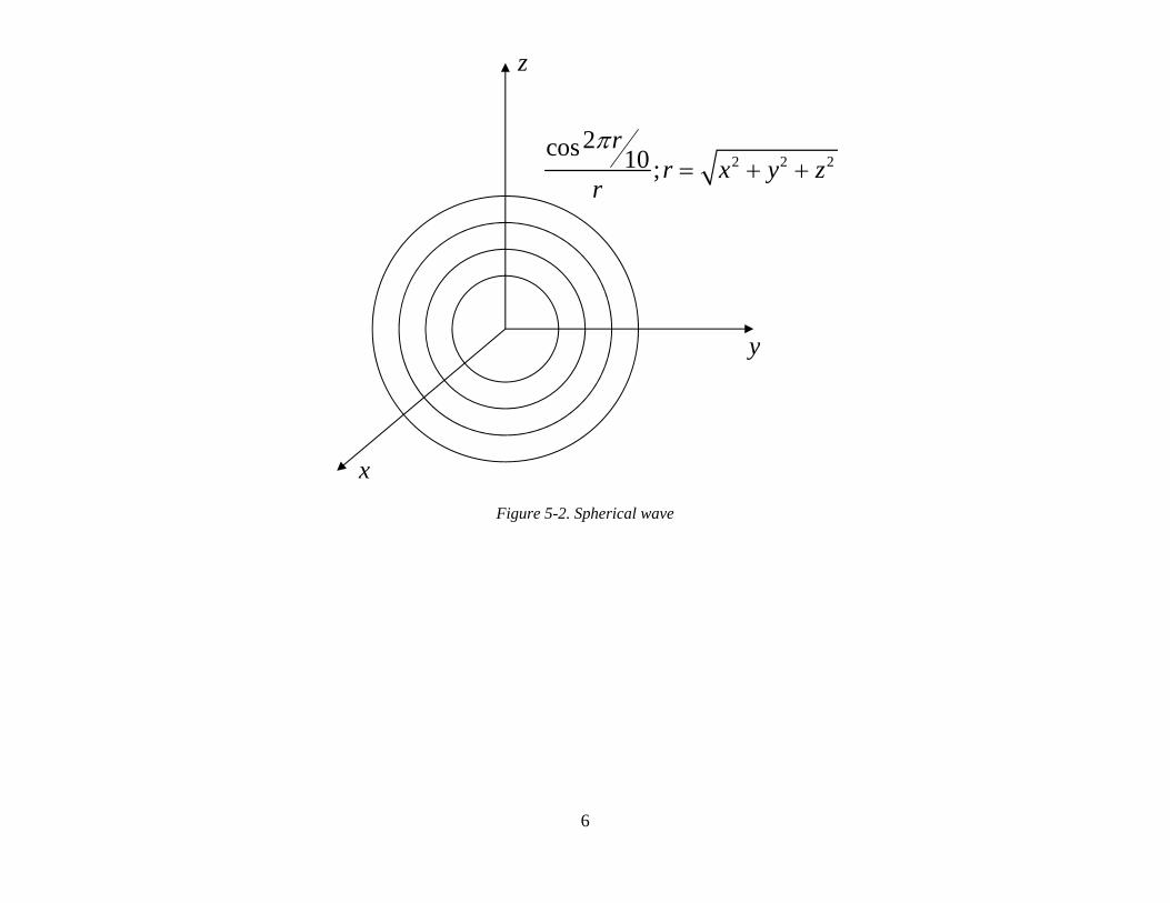
, , 0ikreh r rr
(5.15)
This solution defines a (outgoing) spherical wave.
6
cos2r10
r;r x2 y2 z2
z
x
y
Figure 5-2. Spherical wave
Chapter 6 – Fourier Optics
Gabriel Popescu
University of Illinois at Urbana‐Champaigny p gBeckman Institute
Quantitative Light Imaging Laboratory
Electrical and Computer Engineering, UIUCPrinciples of Optical Imaging
Quantitative Light Imaging Laboratoryhttp://light.ece.uiuc.edu
3.10 Lens as a phase transformer
ECE 460 – Optical Imaging
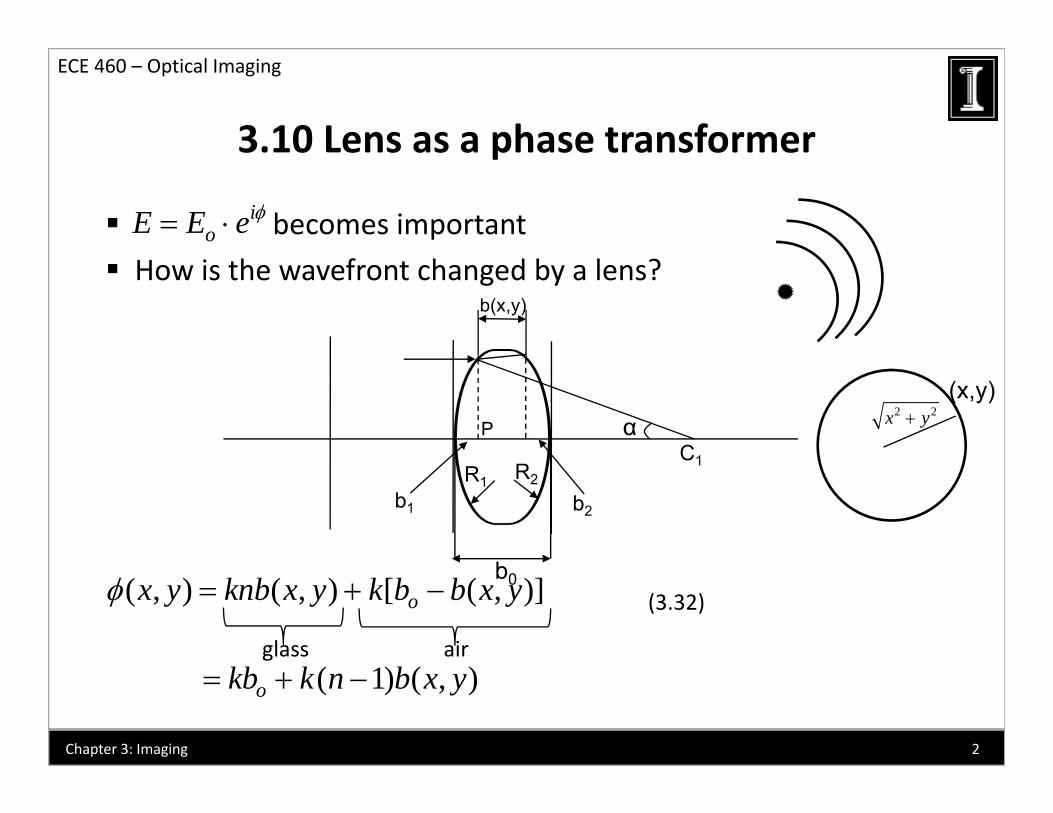
becomes important
3.10 Lens as a phase transformer
ioE E e
How is the wavefront changed by a lens?b(x,y)
C1
αP
(x,y)2 2x y
C1
b1 b2
R1 R2
( , ) ( , ) [ ( , )]ox y knb x y k b b x y
glass air
(3.32)b0
( 1) ( , )okb k n b x y
2Chapter 3: Imaging
3.10 Lens as a phase transformer
ECE 460 – Optical Imaging
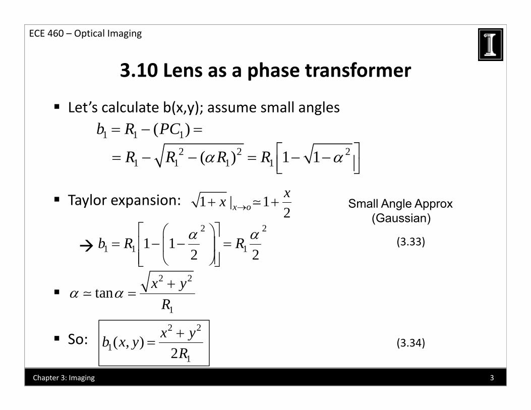
Let’s calculate b(x,y); assume small angles
3.10 Lens as a phase transformer
( )b R PC1 1 1( )b R PC 2 2 2
1 1 1 1( ) 1 1R R R R
Taylor expansion: 1 | 12x oxx
2 2
Small Angle Approx(Gaussian)
2 2
1 1 11 12 2
b R R
2 2x y
(3.33)
S
1tan x y
R
2 2x y So: 1
1( , )
2x yb x y
R
(3.34)
3Chapter 3: Imaging
3.10 Lens as a phase transformer
ECE 460 – Optical Imaging
3.10 Lens as a phase transformer
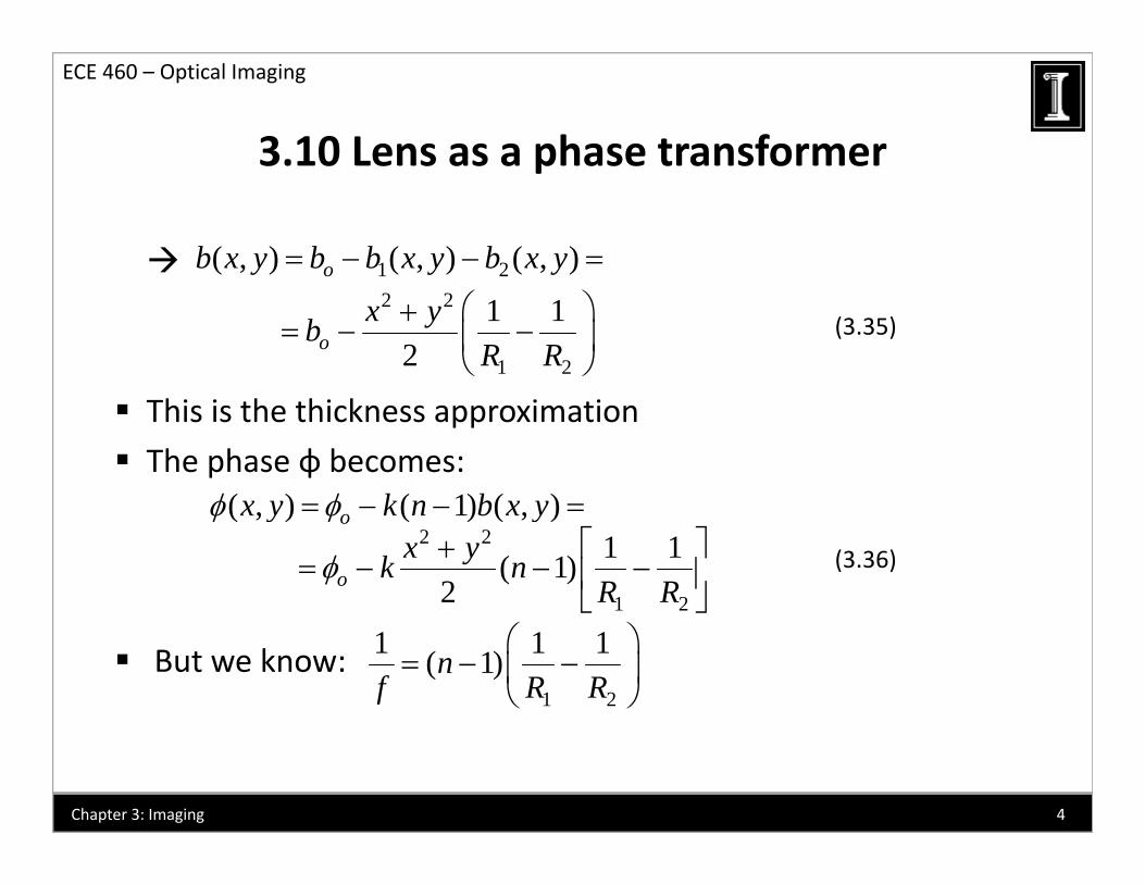
1 2( , ) ( , ) ( , )ob x y b b x y b x y 1 2o
(3.35)2 2
1 2
1 12o
x ybR R
This is the thickness approximation
The phase φ becomes:( ) ( 1) ( )k b ( , ) ( 1) ( , )ox y k n b x y
2 2
1 2
1 1( 1)2o
x yk nR R
(3.36)
But we know:
1 2
1 2
1 1 1( 1)nf R R
4Chapter 3: Imaging
3.10 Lens as a phase transformer
ECE 460 – Optical Imaging
3.10 Lens as a phase transformer
k
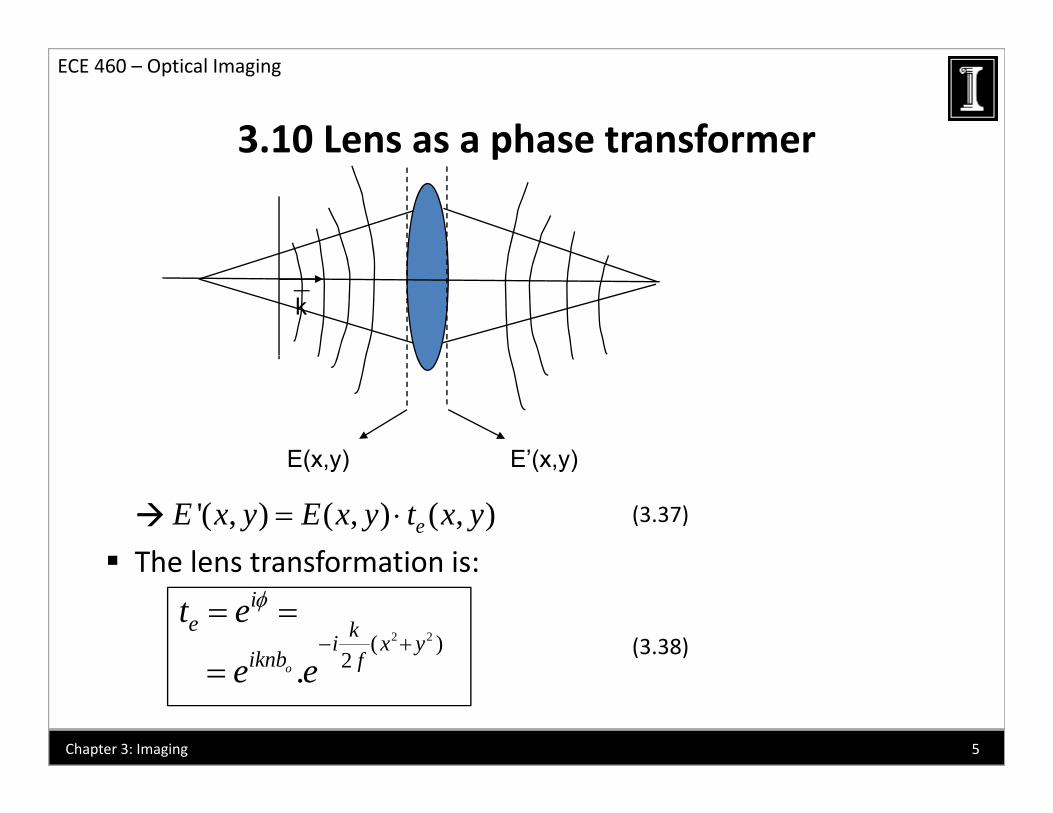
E(x y) E’(x y)
The lens transformation is:
'( , ) ( , ) ( , )eE x y E x y t x y (3.37)
E(x,y) E (x,y)
The lens transformation is:i
et e 2 2( )
2ki x y
iknb f (3.38)2.oiknb fe e
5Chapter 3: Imaging
3.10 Lens as a phase transformer
ECE 460 – Optical Imaging
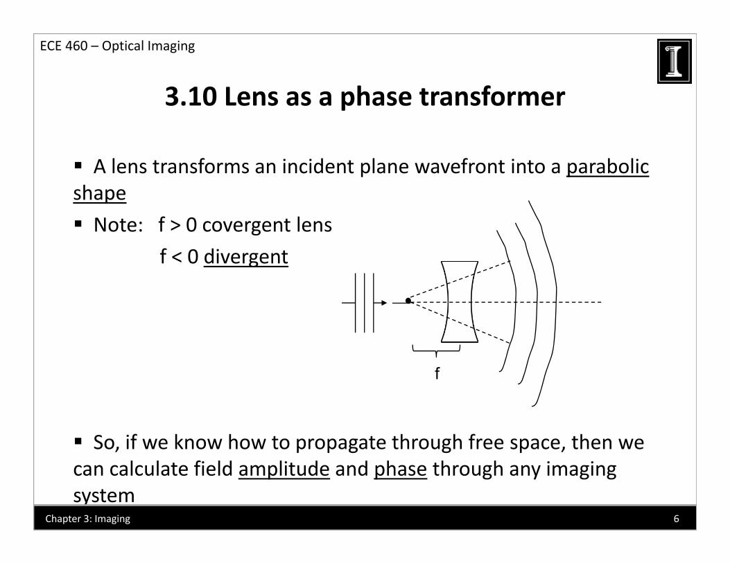
A lens transforms an incident plane wavefront into a parabolic
3.10 Lens as a phase transformer
p pshape
Note: f > 0 covergent lens
f < 0 divergent
f
So, if we know how to propagate through free space, then we can calculate field amplitude and phase through any imaging system
6Chapter 3: Imaging
3.11 Huygens‐Fresnel principle
ECE 460 – Optical Imaging
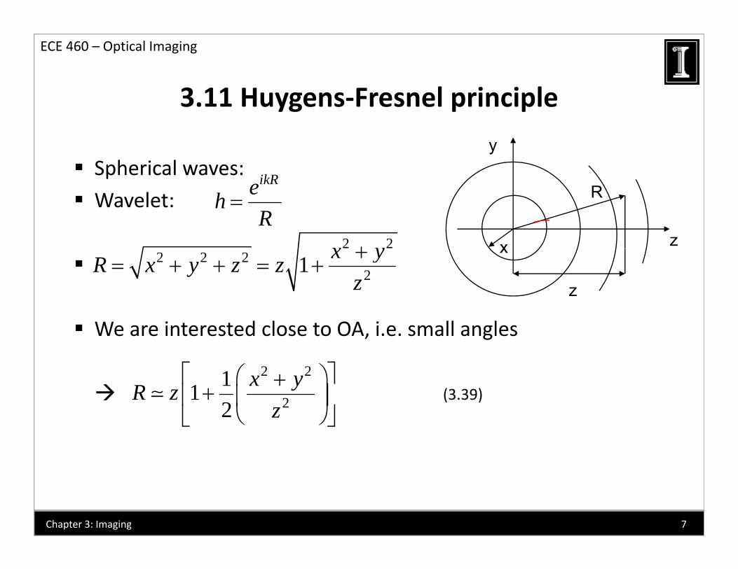
Spherical waves:
3.11 Huygens Fresnel principle
ikR
yp
Wavelet: ikRehR
2 2x y zx
R
2 2 221 x yR x y z z
z
x
z
We are interested close to OA, i.e. small angles
2 211 x yR z
(3 39) 21
2R z
z
(3.39)
7Chapter 3: Imaging

3.11 Huygens‐Fresnel principle
ECE 460 – Optical Imaging
For amplitude is OK
3.11 Huygens Fresnel principle
1 1R z ikRe
R For phase
2 2
211 x ykR kzz z
R z
R
The wavelet becomes:2 2( )2( )
k x yikz izeh
(3 40a) 2 2( )f x y x y
z
Remember, for the lens we found:
2( , ) zh x y ez
(3.40a) ( , )f x y x y 2( )f x x
Free space acts on the wavefront like a divergent lens
2 2( )2( , ) o
ki x yi f
et x y e e
(3.40b)Negative Lens
Free space acts on the wavefront like a divergent lens
(note “+” sign in phase)8Chapter 3: Imaging
3.11 Huygens‐Fresnel principle
ECE 460 – Optical Imaging
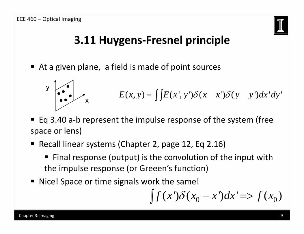
At a given plane, a field is made of point sources
3.11 Huygens Fresnel principle
( , ) ( ', ') ( ') ( ') ' 'E x y E x y x x y y dx dy y
x
Eq 3.40 a‐b represent the impulse response of the system (free space or lens)
x
space or lens)
Recall linear systems (Chapter 2, page 12, Eq 2.16)
Final response (output) is the convolution of the input with p ( p ) pthe impulse response (or Greeen’s function)
Nice! Space or time signals work the same!
9Chapter 3: Imaging
0 0( ') ( ') ' ( )f x x x dx f x
3.11 Huygens‐Fresnel principle
ECE 460 – Optical Imaging
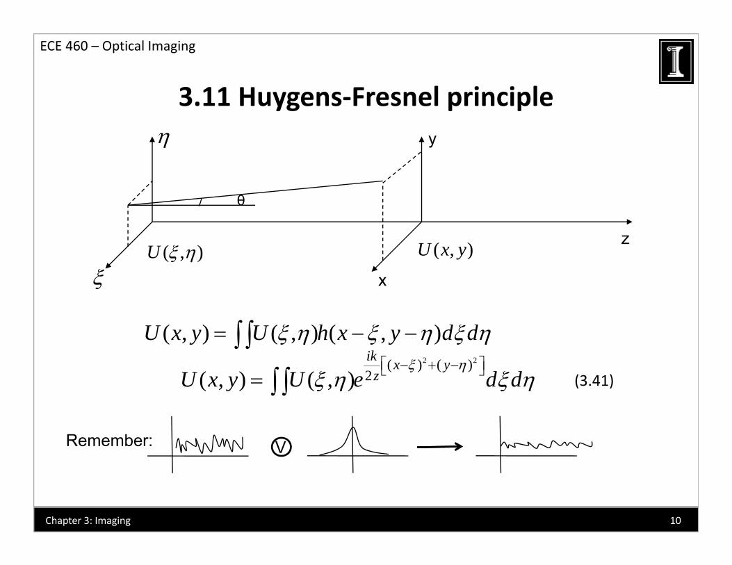
3.11 Huygens Fresnel principley
z
θ
( )U ( )Ux
( , )U ( , )U x y
( , ) ( , ) ( , )U x y U h x y d d 2 2( ) ( )
2( , ) ( , )ik x yzU x y U e d d
(3.41)( , ) ( , )y
VRemember:
10Chapter 3: Imaging
3.11 Huygens‐Fresnel principle
ECE 460 – Optical Imaging
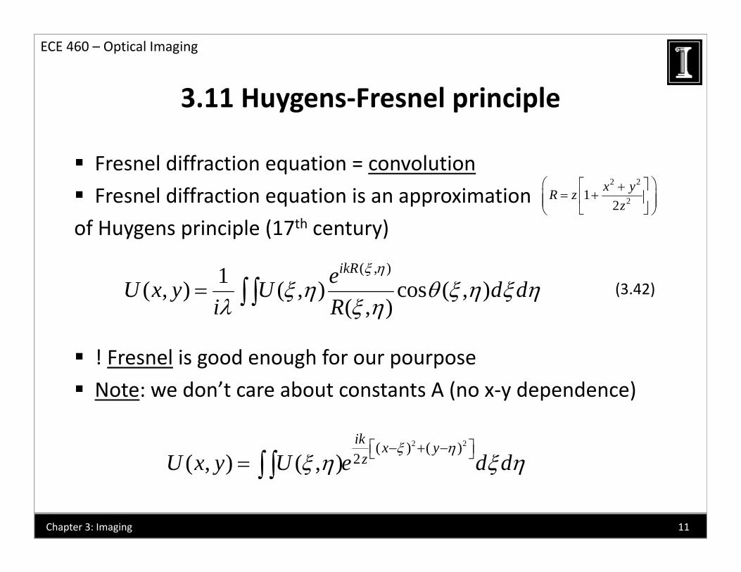
Fresnel diffraction equation = convolution
3.11 Huygens Fresnel principle
Fresnel diffraction equation is an approximation
of Huygens principle (17th century)
2 2
212
x yR zz
( , )1( , ) ( , ) cos ( , )( , )
ikReU x y U d di R
(3.42)
! Fresnel is good enough for our pourpose
Note: we don’t care about constants A (no x‐y dependence)Note: we don t care about constants A (no x y dependence)
2 2( ) ( )2( ) ( )ik x yzU x y U e d d
( , ) ( , )U x y U e d d
11Chapter 3: Imaging
3.12 Fraunhofer Approximation
ECE 460 – Optical Imaging
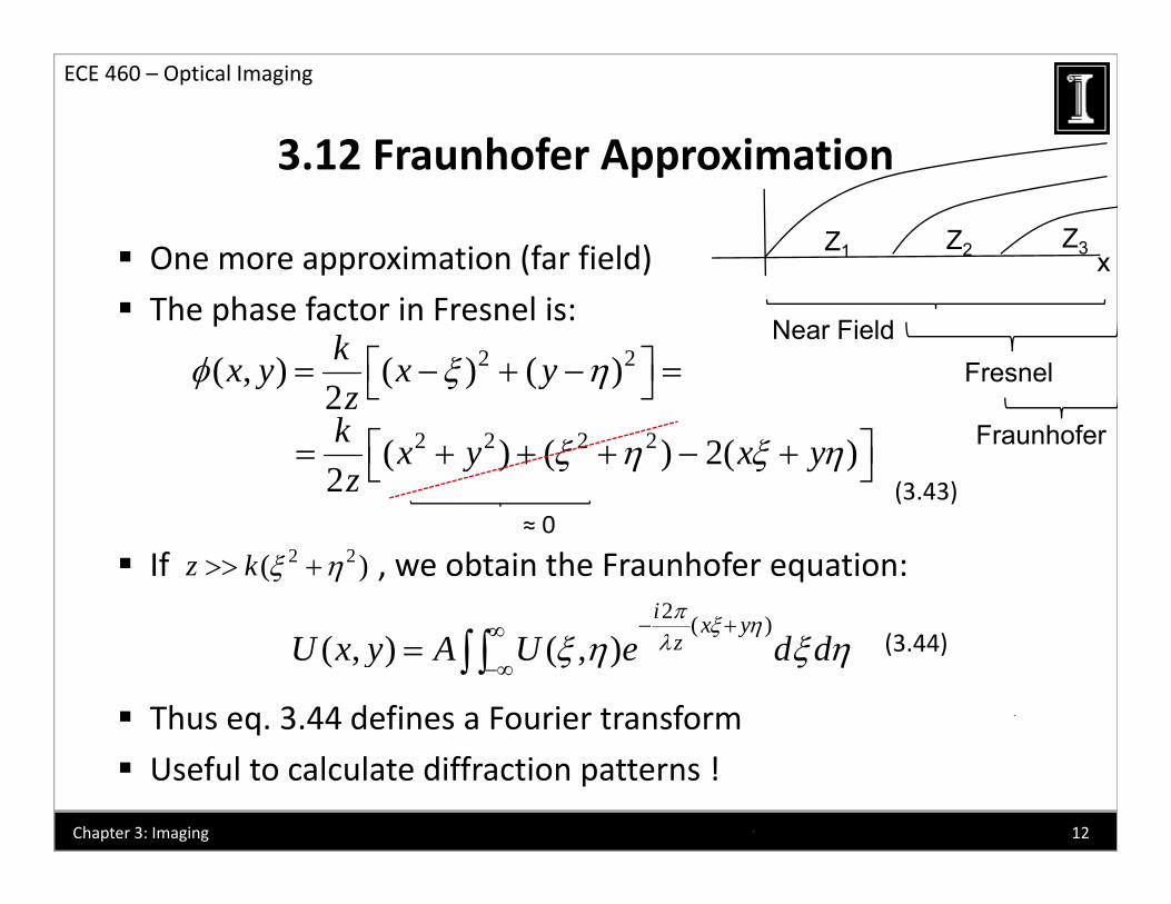
One more approximation (far field)
3.12 Fraunhofer Approximation
Z1 Z2 Z3 x
The phase factor in Fresnel is:2 2( , ) ( ) ( )
2kx y x yz
Near FieldFresnel
2z 2 2 2 2( ) ( ) 2( )
2k x y x yz
(3.43)
Fraunhofer
If , we obtain the Fraunhofer equation:2 2( )z k ≈ 0
2 ( )i x y
Thus eq. 3.44 defines a Fourier transform
( )( , ) ( , )
x yzU x y A U e d d
(3.44)
Useful to calculate diffraction patterns !
12Chapter 3: Imaging
3.12 Fraunhofer Approximation
ECE 460 – Optical Imaging
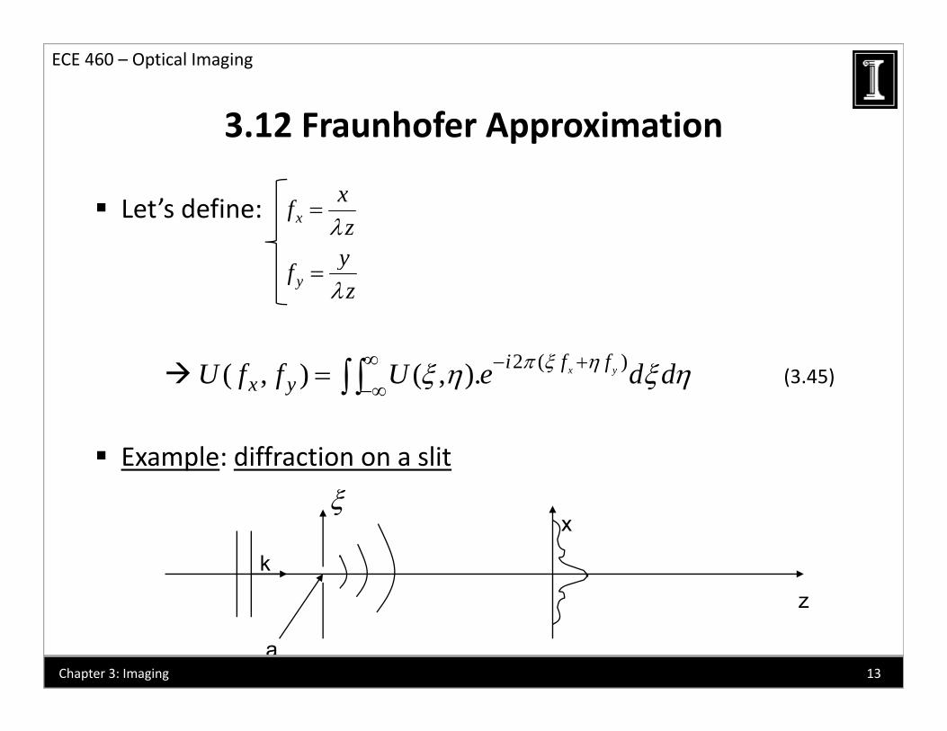
Let’s define:
3.12 Fraunhofer Approximation
xxfz
y
zyfz
2 ( )( , ) ( , ). x yi f fx yU f f U e d d
(3.45)
Example: diffraction on a slit
k
x
z
a13Chapter 3: Imaging
3.12 Fraunhofer Approximation
ECE 460 – Optical Imaging
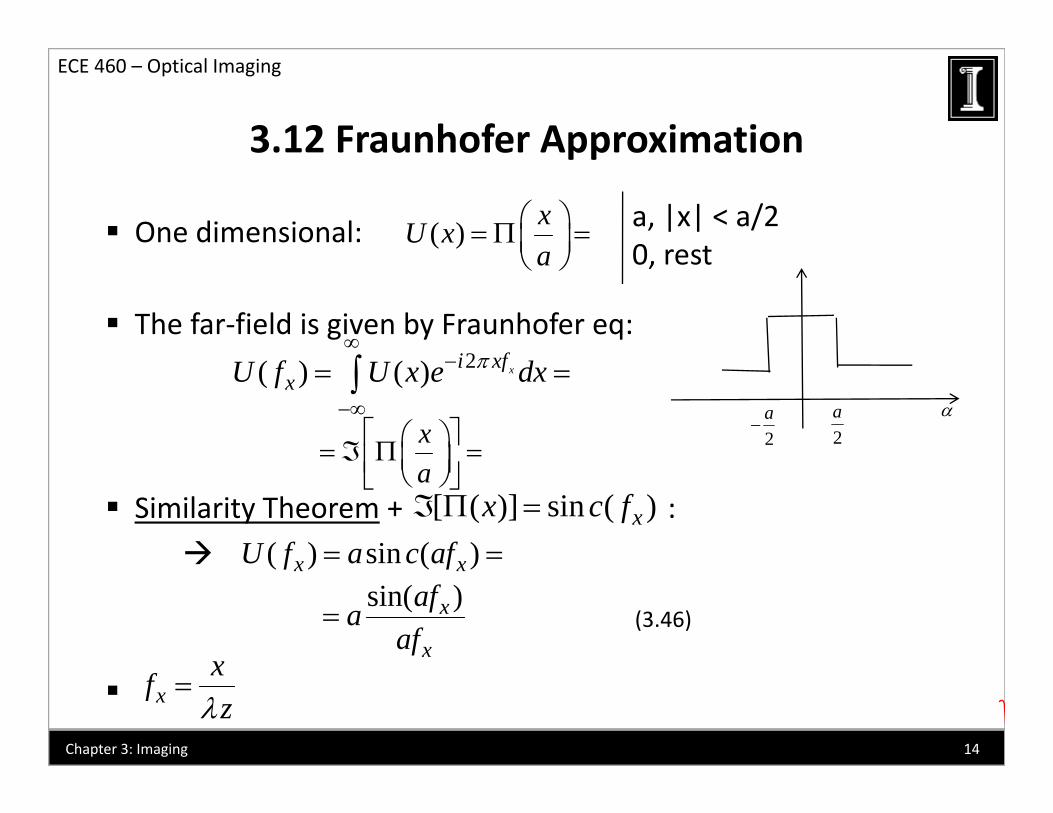
One dimensional:
3.12 Fraunhofer Approximation
( ) xU xa
a, |x| < a/20 rest
The far‐field is given by Fraunhofer eq:
a 0, rest
2i f
2( ) ( ) xi xfxU f U x e dx
x
2a
2a
Similarity Theorem + :
a
[ ( )] sin ( )xx c f ( ) sin ( )U f a c af ( ) sin ( )x xU f a c af
sin( )x
x
afaaf
(3.46)
x x
xfz
14Chapter 3: Imaging
3.12 Fraunhofer Approximation
ECE 460 – Optical Imaging
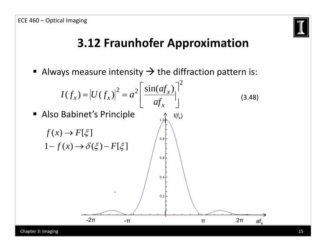
Always measure intensity the diffraction pattern is:
3.12 Fraunhofer Approximation
22 2 sin( )( ) ( ) x
x xx
afI f U f aaf
(3.48)
I(fx) Also Babinet’s Principle
( ) [ ]f x F 1 ( ) ( ) [ ]f x F
-π-2π 2ππ afx15Chapter 3: Imaging
3.12 Fraunhofer Approximation
ECE 460 – Optical Imaging
3.12 Fraunhofer Approximation
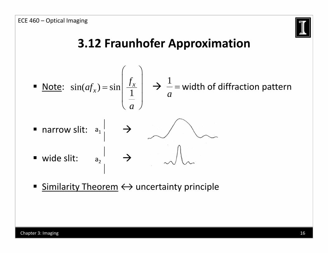
f 1
Note: width of diffraction patternsin( ) sin 1x
xfaf
a
1a
narrow slit: a1
wide slit: a2
Similarity Theorem↔ uncertainty principle
16Chapter 3: Imaging
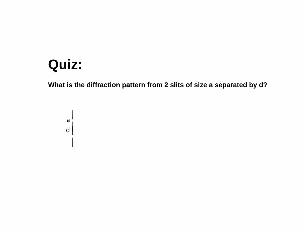
Quiz:What is the diffraction pattern from 2 slits of size a separated by d?
a
dd
3.13 Fourier Properties of lenses
ECE 460 – Optical Imaging
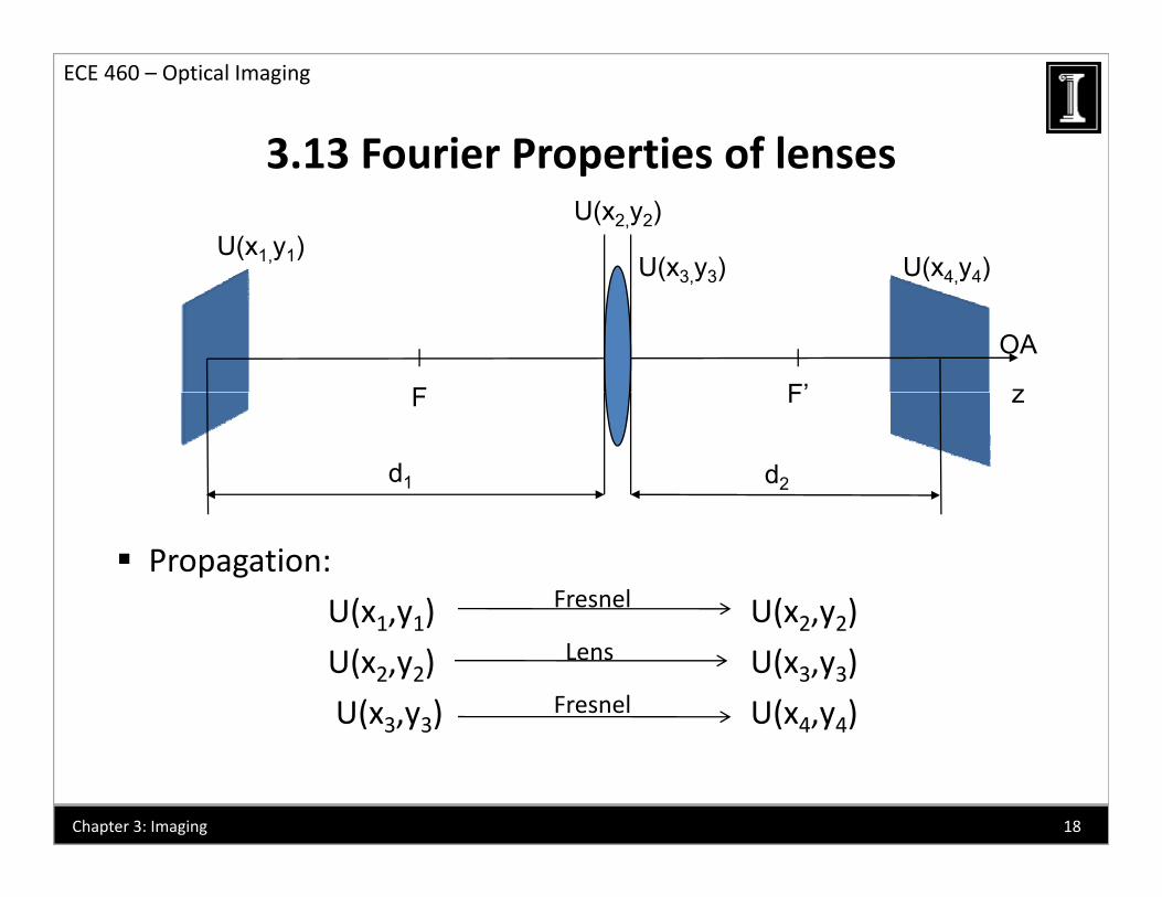
3.13 Fourier Properties of lenses
U(x1,y1)U(x2,y2)
U(x3 y3) U(x4 y4)
F F’
( 3,y3)
OA
z
( 4,y4)
F F z
d1 d2
Propagation:
U(x1,y1) U(x2,y2)FresnelU(x1,y1) U(x2,y2)
U(x2,y2) U(x3,y3)
U(x3,y3) U(x4,y4)Fresnel
Lens
3 3 4 4
18Chapter 3: Imaging
3.13 Fourier Properties of lenses
ECE 460 – Optical Imaging
3.13 Fourier Properties of lenses
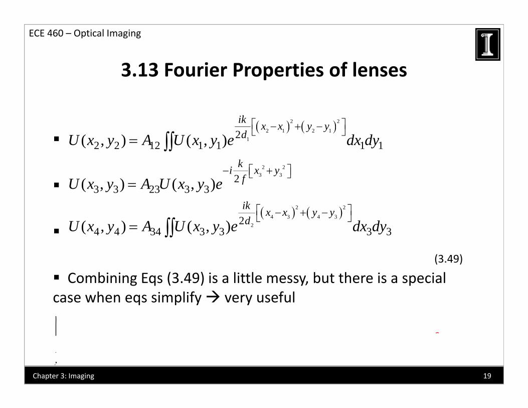
2 2ik x x y y
2 1 2 11
2 23 3
22 2 12 1 1 1 1
2
( , ) ( , )
( ) ( )
x x y yd
ki x yf
U x y A U x y e dx dy
2 2
4 3 4 32
23 3 23 3 3
24 4 34 3 3 3 3
( , ) ( , )
( , ) ( , )
f
ik x x y yd
U x y A U x y e
U x y A U x y e dx dy
Combining Eqs (3.49) is a little messy, but there is a special
4 4 34 3 3 3 3( , ) ( , )U x y A U x y e dx dy(3.49)
Combining Eqs (3.49) is a little messy, but there is a special case when eqs simplify very useful
19Chapter 3: Imaging
3.13 Fourier Properties of lenses
ECE 460 – Optical Imaging
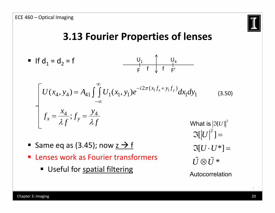
If d1 = d2 = f
3.13 Fourier Properties of lenses
U1 U4
1 12 ( )4 4 41 1 1 1 1 1( ) ( ) x yi x f y fU x y A U x y e dx dy
(3 50)
F F’f f
4 4 41 1 1 1 1 1
4 4
( , ) ( , )
;x y
U x y A U x y e dx dy
x yf ff f
(3.50)
2
Same eq as (3 45); now z f
x yf ff f What is 2[ ]U
2[ ][ *]UU U
Same eq as (3.45); now z f Lenses work as Fourier transformers
Useful for spatial filtering
[ *]*
U UU U
Autocorrelation
20Chapter 3: Imaging
Autocorrelation
3.13 Fourier Properties of lenses
ECE 460 – Optical Imaging
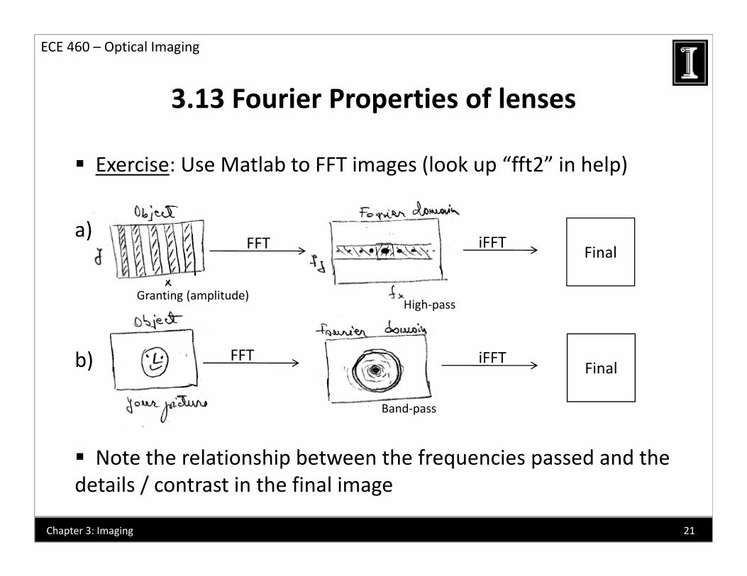
Exercise: Use Matlab to FFT images (look up “fft2” in help)
3.13 Fourier Properties of lenses
a)FFT iFFT
FinalFinal
Granting (amplitude)High‐pass
b) FFT iFFTFinal
Note the relationship between the frequencies passed and the
Band‐pass
details / contrast in the final image
21Chapter 3: Imaging
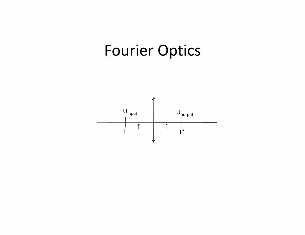
Fourier Optics
Uinput
F
Uoutput
F’f f
F F
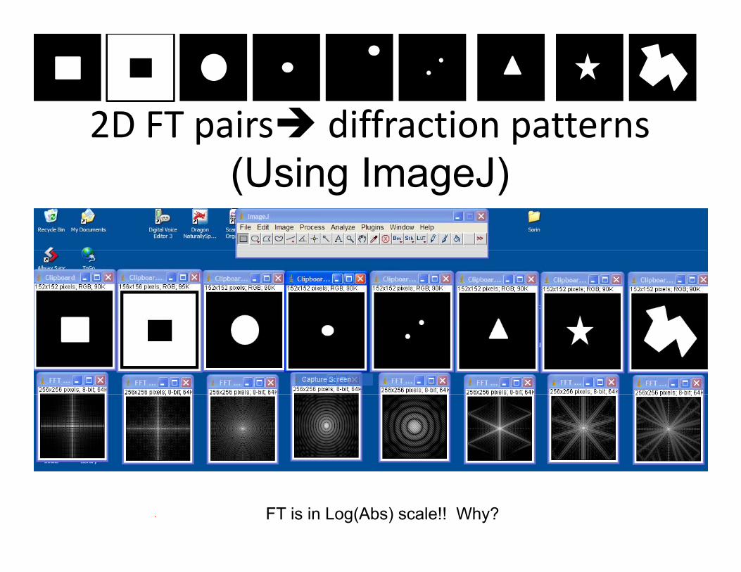
2D FT pairs diffraction patterns(Using ImageJ)(Using ImageJ)
FT is in Log(Abs) scale!! Why?
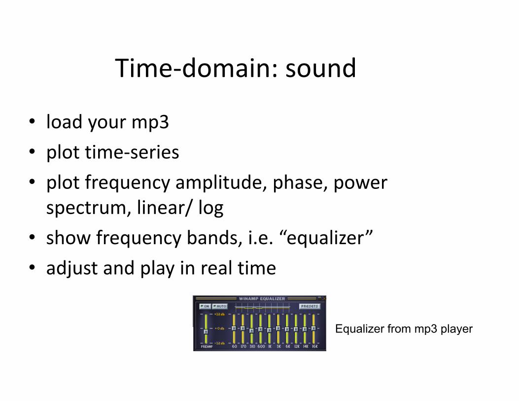
Time‐domain: soundTime domain: sound
• load your mp3load your mp3
• plot time‐series
l f li d h• plot frequency amplitude, phase, power spectrum, linear/ log
• show frequency bands, i.e. “equalizer”
• adjust and play in real timej p y
Equalizer from mp3 playerEqualizer from mp3 player
Space‐domain: image
• load your image
Space domain: image
load your image
• display image
h 2 f li d h• show 2D frequency amplitude, phase, power spectrum, linear/ log
• show rings of equal freq., “image equalizer”
• adjust and display in real time‐ example on j p y pnext slide
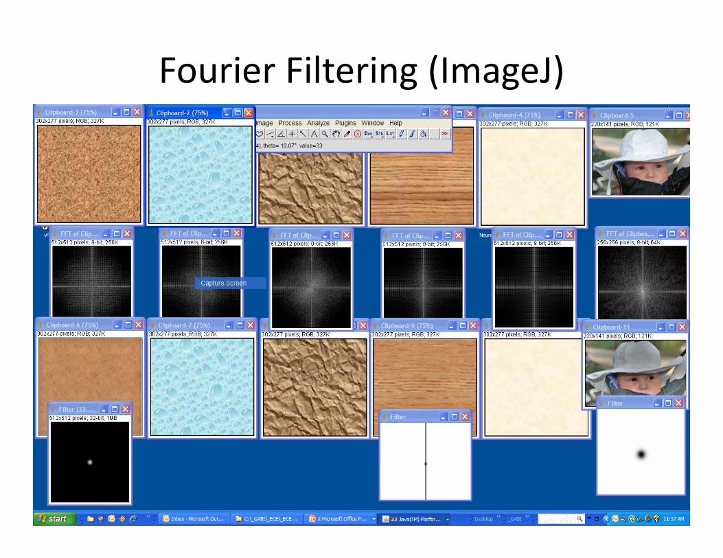
Fourier Filtering (ImageJ)