Embed Size (px)
Citation preview
Finite Key Analysis in Quantum Cryptography
Inaugural-Dissertation
zur
Erlangung des Doktorgrades der
Mathematisch-Naturwissenschaftlichen Fakultat
der Heinrich-Heine-Universitat Dusseldorf
vorgelegt von
Tim Meyer
aus Neustadt am Rubenberge
Oktober 2007
Aus dem Institut fur Theoretische Physik, Lehrstuhl III
der Heinrich-Heine Universitat Dusseldorf
Gedruckt mit der Genehmigung der
Mathematisch-Naturwissenschaftlichen Fakultat der
Heinrich-Heine-Universitat Dusseldorf
Referent: Prof. Dr. D. Bruß
Koreferent: Prof. Dr. R. Egger
Tag der mundlichen Prufung: 31. Oktober 2007
“Die grundlegende Theorie [der Quantenkryptographie] ist [. . . ] schon
geklart. Die Theoriefragen beziehen sich heute hauptsachlich auf die
Fragen der Sicherheit, es geht dabei beispielsweise um grundsatzliche
Sicherheitsbeweise der Systeme. Was interessanterweise bei unseren
Methoden etwas ist, das wir nicht benotigen.
Es gibt verschiedene Moglichkeiten, physisch diese Quantenverbindun-
gen, die dann die Schlussel austauschen, zur Verschlusselung zu real-
isieren. Wir machen das auf eine Art, bei der die Sicherheit offenkundig
ist, dazu brauchen wir nicht einmal einen Beweis.”
O. Univ.-Prof. Dr. phil. Anton Zeilinger, e&i, Heft 5 2007

Abstract
In view of experimental realization of quantum key distribution schemes, the study of
their efficiency becomes as important as the proof of their security. The latter is the
subject of most of the theoretical work about quantum key distribution, and many
important results such as the proof of unconditional security have been obtained. The
efficiency and also the robustness of quantum key distribution protocols against noise
can be measured by figures of merit such as the secret key rate (the fraction of input
signals that make it into the key) and the threshold quantum bit error rate (the maximal
error rate such that one can still create a secret key). It is important to determine
these quantities because they tell us whether a certain quantum key distribution scheme
can be used at all in a given situation and if so, how many secret key bits it can
generate in a given time. However, these figures of merit are usually derived under
the “infinite key limit” assumption, that is, one assumes that an infinite number of
quantum states are send and that all sub-protocols of the scheme (in particular privacy
amplification) are carried out on these infinitely large blocks. Such an assumption
usually eases the analysis, but also leads to (potentially) too optimistic values for the
quantities in question.
In this thesis, we are explicitly avoiding the infinite key limit for the analysis of
the privacy amplification step, which plays the most important role in a quantum key
distribution scheme. We still assume that an optimal error correction code is applied
and we do not take into account any statistical errors that might occur in the param-
eter estimation step. In [1], Renner and coworkers derived an explicit formula for the
obtainable key rate in terms of Renyi entropies of the quantum states describing Alice’s,
Bob’s, and Eve’s systems. This results serves as a starting point for our analysis, and
we derive an algorithm that efficiently computes the obtainable key rate for any finite
number of input signals, without making any approximations.
As an application, we investigate the so-called “Tomographic Protocol” [2, 3], which
is based on the Six-State Protocol [4, 5] and where Alice and Bob can obtain the ad-
ditional information which quantum state they share after the distribution step of the
5
protocol. We calculate the obtainable secret key rate under the assumption that the
eavesdropper only conducts collective attacks and give a detailed analysis of the depen-
dence of the key rate on various parameters: The number of input signals (the block
size), the error rate in the sifted key (the QBER), and the security parameter. Further-
more, we study the influence of multi-photon events which naturally occur in a realistic
implementation.

Zusammenfassung
Im Zuge der experimentellen Realisierung von Protokollen zur quantenmechanischen
Schlusselverteilung wird die Analyse ihrer Effizienz genauso wichtig wie der Beweis ihrer
Sicherheit. Letzteres ist das Thema der meisten theoretischen Arbeiten auf diesem
Gebiet, welche wichtige Ergebnisse lieferten, wie etwa der Beweis der unbedingten
Abhorsicherheit. Die Effizienz und die Robustheit eines Protokolls lassen sich durch
Gutekriterien wie die Schlusselrate (der Bruchteil der gesendeten Signale, die den Schlus-
sel bilden) oder die Schwellen-Quantenfehlerrate (die maximale tolerierbare Fehlerrate,
bei der die Schlusselerzeugung noch moglich ist) definieren. Diese Großen mussen bes-
timmt werden, um fur ein gegebenes Szenario festzustellen, ob ein gewisses Protokoll
uberhaupt anwendbar ist und wenn ja, wieviele Bits sicherer Schlussel generiert werden
konnen. Im Allgemeinen jedoch konnen diese Gutekriterien nur unter der Annahme
berechnet werden, dass alle Zwischenschritte des Protokolls — insbesondere der pri-
vacy amplification-Schritt — mit unendlich vielen Signalen arbeiten. Diese Annahme
erleichtert die Analyse zwar, allerdings werden dadurch moglicherweise zu optimitische
Werte fur die Gutekriterien errechnet.
Aus diesem Grund vermeiden wir in dieser Arbeit die Annahme der unendlich
vielen Signale fur den privacy amplification-Schritt, welcher der wichtigste in einem
Schlusselverteilungsprotokoll ist. Jedoch nehmen wir weiterhin an, dass nur optimale
Fehlerkorrekturcodes verwendet werden und wir berucksichtigen auch keine statistischen
Fehler, die im Parameter-Abschatzungsschritt auftreten konnen. In [1] haben Renner
et al. eine explizite Formel fur die erreichbare Schlusselrate bzgl. Renyi-Entropien der
Quanten-Zustande, die Alices, Bobs und Eves Quanten-System beschreiben, ermittelt.
Dieses Ergebnis ist der Ausgangspunkt fur unsere Analyse, in der wir einen Algorith-
mus entwickeln, welcher die erreichbare Schlusselrate fur jegliche Anzahl von Signalen
effizient berechnet, ohne auf Naherungen zuruckzugreifen.
Als eine Anwendung betrachten wir das sogenannte “Tomographische Protokoll” [2,
3], welches auf dem Six-State-Protokoll [4, 5] basiert, und in welchem Alice und Bob
zusatzlich bestimmen konnen, welchen Quantenzustand sie sich nach dem Verteilungss-

chritt des Protokolls teilen. Wir berechnen die erreichbare Schlusselrate unter der An-
nahme, dass Eve nur kollektive Attacken durchfuhrt und analysieren detailliert, auf
welche Weise die Schlusselrate von folgenden Parametern abhangt: Die Anzahl der Ein-
gangssignale (die Blocklange), die Fehlerrate im “gesiebten” Schlussel (die QBER) und
der Sicherheitsparameter. Außerdem untersuchen wir den Einfluß von Mehr-Photonen-
Signalen, welche in jeder realistischen Anwendung auftreten.
Contents
1 Introduction 11
1.1 Secret Communication . . . . . . . . . . . . . . . . . . . . . . . . . . . . 11
1.2 Quantum Key Distribution . . . . . . . . . . . . . . . . . . . . . . . . . 13
1.3 Efficiency of Quantum Key Distribution . . . . . . . . . . . . . . . . . . 17
1.4 Summary of the Main Results . . . . . . . . . . . . . . . . . . . . . . . . 18
1.5 Outline of This Work . . . . . . . . . . . . . . . . . . . . . . . . . . . . . 20
2 Preliminaries 23
2.1 Classical World . . . . . . . . . . . . . . . . . . . . . . . . . . . . . . . . 23
2.2 Quantum World . . . . . . . . . . . . . . . . . . . . . . . . . . . . . . . 24
3 Quantum Key Distribution Protocols 27
3.1 Composition of a QKD Protocol . . . . . . . . . . . . . . . . . . . . . . 27
3.2 Quantum Part/Distribution of Quantum States . . . . . . . . . . . . . . 30
3.2.1 Prepare-and-measure Schemes . . . . . . . . . . . . . . . . . . . 30
3.2.2 Entanglement-based Schemes . . . . . . . . . . . . . . . . . . . . 32
3.2.3 Equivalence of Entanglement-based and Prepare-and-measure. . . 33
3.2.4 Eavesdropping . . . . . . . . . . . . . . . . . . . . . . . . . . . . 34
3.3 Classical Part . . . . . . . . . . . . . . . . . . . . . . . . . . . . . . . . . 35
3.3.1 Measurement . . . . . . . . . . . . . . . . . . . . . . . . . . . . . 35
3.3.2 Parameter Estimation . . . . . . . . . . . . . . . . . . . . . . . . 36
3.3.3 Pre-processing . . . . . . . . . . . . . . . . . . . . . . . . . . . . 36
3.3.4 Information Reconciliation . . . . . . . . . . . . . . . . . . . . . 36
3.3.5 Privacy Amplification. . . . . . . . . . . . . . . . . . . . . . . . . 37
4 Security of Quantum Key Distribution 39
4.1 Security in the Classical World . . . . . . . . . . . . . . . . . . . . . . . 39
4.2 Security in the Quantum World . . . . . . . . . . . . . . . . . . . . . . . 40
9
Contents
4.3 Classification of Eavesdropping Strategies . . . . . . . . . . . . . . . . . 42
4.4 The Role of Purifications . . . . . . . . . . . . . . . . . . . . . . . . . . 43
4.4.1 Purifications in QKD . . . . . . . . . . . . . . . . . . . . . . . . 43
4.4.2 On the (Im)possibility of Physical Purification . . . . . . . . . . 44
5 Privacy Amplification 47
5.1 Introduction . . . . . . . . . . . . . . . . . . . . . . . . . . . . . . . . . . 47
5.2 Privacy Amplification in the Quantum World . . . . . . . . . . . . . . . 49
5.3 Smooth Renyi Entropies . . . . . . . . . . . . . . . . . . . . . . . . . . . 52
5.3.1 General Properties . . . . . . . . . . . . . . . . . . . . . . . . . . 52
5.3.2 Simplifications for Sε2 and Sε
0 . . . . . . . . . . . . . . . . . . . . 53
5.3.3 Explicit Calculation of Sε2, S
ε0, and Hε
0 . . . . . . . . . . . . . . . 56
5.3.4 Additivity . . . . . . . . . . . . . . . . . . . . . . . . . . . . . . . 64
6 Finite Key Analysis for the Tomographic Protocol 67
6.1 Description of the Protocol . . . . . . . . . . . . . . . . . . . . . . . . . 68
6.2 Privacy Amplification for Finite Block Size . . . . . . . . . . . . . . . . 71
6.3 Results for Single-Copy Signal States . . . . . . . . . . . . . . . . . . . . 73
6.4 Inclusion of Multi-Photon Events . . . . . . . . . . . . . . . . . . . . . . 81
6.4.1 Concept . . . . . . . . . . . . . . . . . . . . . . . . . . . . . . . . 83
6.4.2 Symmetric Splitting . . . . . . . . . . . . . . . . . . . . . . . . . 86
6.4.3 Asymmetric Splitting . . . . . . . . . . . . . . . . . . . . . . . . 89
6.4.4 Decoy States . . . . . . . . . . . . . . . . . . . . . . . . . . . . . 91
7 Conclusion 95
A Numerical methods 97
10
Chapter 1
Introduction
Quantum key distribution has taken the step from a theoretician’s mind to experimental
implementation, becoming a commercial product [6, 7]. During the last basic models
which barely described the real world, culminating in the proof of universal composabil-
ity and security under the most general circumstances. Besides these conceptual proofs
it is necessary to investigate the performance of protocols. What rate of secret key bits
can be generated by a specific setup? The answer to this question certainly depends
on the type of equipment that is used in the actual implementation. A performance
measure which only depends on the underlying protocol is given by the number of secret
key bits per quantum signal sent. The main subject of this thesis is to compute such
a figure of merit (the secret key rate) for a restricted class of quantum key distribution
protocols.
1.1 Secret Communication
The ability to secretly communicate has always been of great importance in many aspects
of our life: Already in 500 B.C., the Spartans invented a cryptographic device called
scytale [8]. This is a wooden rod around which one wraps a strap of leather or parchment.
Afterwards, the message which is to be encrypted (also called plain text) is written onto
the strap such that each letter appears on a new twist. Then the strap is unwrapped, now
showing only incoherent letters, and is transported to the receiver who owns a scytale
of the same diameter to decode the message. The scytale implements an encryption
method known as shift cipher, in which every letter of the plain text gets shifted by a
fixed amount. Another example is the Caesar cipher [9], invented by the Roman emperor
in 50 B.C., in which letters of the plain text alphabet are replaced by certain other letters.
Such a simple scrambling of the plain text renders a message unreadable, at least at first
11
1.1. Secret Communication
glance, but 2000 years ago this was apparently enough to scare off adversaries. Ever
since then, cryptography (the science of code making) and cryptoanalysis (the science of
code breaking) are two fields constantly feeding each other: Whenever some encryption
scheme gets broken, cryptographers are forced to invent a new code, being even harder
to break. This in turn encourages code breakers to search for flaws in this new scheme.
Eventually, this mutual outperforming has led to the situation we are facing today: The
search for an encryption method which is inherently secure, thus impossible to break.
RSA
One of the most successful cryptosystems used today is the RSA system, named after
its inventors Rivest, Shamir, and Adleman [10]. It is an asymmetric cryptosystem,
employing two keys, a private and a public one. The public key (as the name suggests)
is announced to everybody who might be willing to communicate secretly with the holder
of the private key, which is kept secret. Mathematically, the scheme is based on so-called
(trap door) one-way functions [11], which are easy to compute (using the public key), but
hard to invert, unless one possesses some kind of “trap door” information, the private
key. In this way it is guaranteed that, only having access to the public key, everybody
can encrypt messages, but lacking the private key, one cannot decrypt them. However,
the fact that one-way functions are “hard” to invert is merely a matter of observation
rather than a mathematical statement. Being hard to calculate in this sense means that
there has not yet been found any algorithm solving the task in polynomial time. By a
reasonable choice of the size of some input parameters (the key length), one can ensure
that using any known algorithm, computing the plain text from the cipher text while
only knowing the public key becomes unfeasible, as the time needed for these algorithms
to finish can be made arbitrarily large.
Still, there are two problems threatening the applicability of RSA: First, it might
happen that an algorithm is found, which can invert one-way functions in a polynomial
time. Although such a discovery seems unlikely, is has not yet been ruled out by a
rigorous mathematical proof. Second, and possibly more severe, as computer power is
increasing exponentially all times [12], brute force methods becoming more and more
feasible. For instance, older implementation of RSA, using a built-in key length which
appeared to providing enough security a decade ago can potentially be broken these
days.1 Also with the advent of the quantum computer, which might be superior to
1In 1977, it was supposed to take about 40 · 1015 years (one million times the age of the universe)
to break a 425-bit key. In 1994, 1600 computers “only” needed eight months, and nowadays, a single
desktop PC could to the same job. It is recommended today to use at least 2048-bit keys [13].
12
Chapter 1. Introduction
classical algorithms, it is not clear how long it takes until inverting one-way functions
becomes feasible.
Unconditional Security
To provide secure communication which is not suffering the flaw of potentially becoming
insecure at a certain time in the future, a new type of cryptographic application is
needed. We call a scheme unconditionally secure if its security can be mathematically
proven and if it is not based on any assumptions about the adversary’s abilities, such as
being limited in computer power, memory, or time. Fortunately, such a scheme exists:2
The Vernam cipher [14] is used to encrypt messages given in binary notation using a
key consisting of random bits which is as long as the message and shared between the
parties which wish to communicate. Encryption is performed by calculating bitwise
addition modulo two of the plain text and the key, and decryption by adding the cipher
text to the key. It has been shown by Shannon [15] that such a cryptographic scheme
is unconditionally secure if the key is completely random and only used once (and is
of course unknown to the adversary), thus the name “one-time pad”. The proof of its
security is quite intuitive, since the result mi ⊕ ki of the addition of a plain text bit mi
to a key bit ki is completely random if the key bit is completely random. Therefore, the
cipher text bit mi ⊕ ki does not contain any information about the plain text mi, and
consequently the scheme is perfectly secure.
The catch of the one-time pad is the following: Since the key is a random bit string
of the same length as the message, which needs to be generated from scratch for each
message to be sent, one faces the problem of distributing large amounts of data. More-
over, the problem of keeping this key secret remains. In former times, code books where
employed, where pages with used codes were torn out. For state-of-the-art applications,
we need to find a reliable and efficient key distribution scheme.
1.2 Quantum Key Distribution
Quantum Key Distribution (QKD) aims exactly at providing such a distribution scheme
for random keys. To do so, a QKD protocol makes use of a quantum channel connecting
the honest parties, traditionally called Alice and Bob. Through this channel, they can
send quantum systems as they see fit. In a real implementation, this quantum channel
will usually be an optical fiber guiding photons, but our analysis will not assume any
2Actually, exactly one such scheme has been found yet.
13
1.2. Quantum Key Distribution
Eve
Classical channel
Quantum channel
Alice Bob
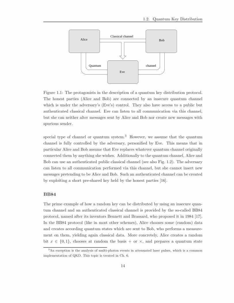
Figure 1.1: The protagonists in the description of a quantum key distribution protocol.
The honest parties (Alice and Bob) are connected by an insecure quantum channel
which is under the adversary’s (Eve’s) control. They also have access to a public but
authenticated classical channel. Eve can listen to all communication via this channel,
but she can neither alter messages sent by Alice and Bob nor create new messages with
spurious sender.
special type of channel or quantum system.3 However, we assume that the quantum
channel is fully controlled by the adversary, personified by Eve. This means that in
particular Alice and Bob assume that Eve replaces whatever quantum channel originally
connected them by anything she wishes. Additionally to the quantum channel, Alice and
Bob can use an authenticated public classical channel (see also Fig. 1.2). The adversary
can listen to all communication performed via this channel, but she cannot insert new
messages pretending to be Alice and Bob. Such an authenticated channel can be created
by exploiting a short pre-shared key held by the honest parties [16].
BB84
The prime example of how a random key can be distributed by using an insecure quan-
tum channel and an authenticated classical channel is provided by the so-called BB84
protocol, named after its inventors Bennett and Brassard, who proposed it in 1984 [17].
In the BB84 protocol (like in most other schemes), Alice chooses some (random) data
and creates according quantum states which are sent to Bob, who performs a measure-
ment on them, yielding again classical data. More concretely, Alice creates a random
bit x ∈ 0, 1, chooses at random the basis + or ×, and prepares a quantum state
3An exception is the analysis of multi-photon events in attenuated laser pulses, which is a common
implementation of QKD. This topic is treated in Ch. 6.
14
Chapter 1. Introduction
|x+〉 = |x〉 in case of the +-basis or |x×〉 = (|0〉 + (−1)x|1〉)/√
2 in case of the ×-basis.
Thus one out of four possible states is sent through the quantum channel. Bob on his
side also chooses one of the two bases + and × at random and performs a measurement
on the arriving quantum state with respect to that basis. His measurement outcome is
some random number y ∈ 0, 1, possibly (hopefully) correlated with the bit x Alice
chose. This procedure is repeated many times, creating a string of bits on Alice’s and
Bob’s side. Assuming a perfect channel (in particular, no eavesdropping), Bob will get
the quantum states sent by Alice undisturbed and we observe that a measurement in an
incompatible basis results in a random bit y, uncorrelated with x. On the other hand,
when Bob measures in the same basis as Alice chose, the outcome y will be equal to x.
In the next step, Alice and Bob announce the bases they used for preparing/measuring
each quantum state via the public channel. They determine the non-matching events
and discard all corresponding bits. If there was no eavesdropping or other noise, they
are now left with an identical, random bit string.
A simple strategy to break this protocol seems to be to simply copy the quantum
states while they are traveling from Alice to Bob. In a classical world, there is nothing
that the honest parties could do about that. In a quantum world however, things look
different (and more promising for the security of key distribution).
The No-Cloning Theorem
It can be viewed as the fundamental concept, rendering quantum key distribution pos-
sible, that non-orthogonal quantum states cannot be copied (or cloned) perfectly. This
is the statement of the No-Cloning Theorem [18], which can be proven in a simple
way: Suppose there exists some unitary operation4 U with U |ψ1〉|0〉 = |ψ1〉|ψ1〉 and
U |ψ2〉|0〉 = |ψ2〉|ψ2〉, where |ψ1,2〉 are two states which are to be cloned and |0〉 is some
arbitrary input state. By taking the scalar products of the left- and right-hand sides of
these equations, it follows that 〈ψ1|ψ2〉 = |〈ψ1|ψ2〉|2, which implies that |ψ1〉 and |ψ2〉are either identical (the trivial case) or orthogonal. For the BB84 protocol this implies
that the adversary cannot perfectly copy the states sent from Alice to Bob, since they
are taken from a set containing non-orthogonal states.
A more general strategy for Eve would be to perform a similar unitary operation
on the input states |ψi〉 and some probe state |0〉, U |ψi〉|0〉 = |ψ′i〉|φi〉 and then try
to distinguish the output probe states |φ〉. By the same argument as above, one can
show that 〈ψ′1|ψ′
2〉〈φ1|φ2〉 is constant, which means that whenever one wants to have
the output states |φi〉 to be more orthogonal, the input states |ψi〉 are getting more
4A unitary operation is the most general way to describe the evolution of a pure quantum state.
15
1.2. Quantum Key Distribution
identical. This means that more distinguishable states probe states come at the cost of
more disturbance of the input states. In this way the eavesdropper runs into the danger
of being detected by Alice and Bob, who can monitor the error rate in their data.
The Role of Entanglement
In 1991, Ekert proposed a QKD protocol not based on sending classical information
encoded into certain quantum systems, but rather on entanglement [19]. The idea of this
protocol is to exploit the correlations one obtains when performing local measurements
on entangled quantum states. In the original work, Alice and Bob aim at distributing
the singlet state |ψ−〉 = (|01〉 − |10〉)/√
2 and then measuring a spin component along
a direction chosen at random from a set of three possible directions. The distribution
and measurements are repeated many times, and afterwards Alice and Bob reveal the
measurement directions they chose. Those are selected such that there exists a common
direction for Alice and Bob, yielding an (anti)correlated string of measurement outcomes
and moreover, using the expectation value for the other directions, one can evaluate some
CHSH inequality [20] (see also [21]). In this way, Alice and Bob can verify whether the
quantum state upon which they performed their measurement was entangled. Ideally,
they would find that they shared the state |ψ−〉, which ensures that the key they draw
from the measurement outcomes is perfectly secure, since the state |ψ−〉 is pure and
cannot be correlated with anything else.
Entanglement theory provides some powerful tools for the understanding of such
“entanglement-based” protocols: Most notably, one can show that whenever Alice and
Bob share a separable state, no secret key can created [22]. If the quantum systems are
qubits, entanglement is even a sufficient condition, which means that entanglement is
equivalent to the possibility of secret key extraction [23]. Surprisingly, it is not enough
to only share the entanglement, Alice and Bob even need to be able to verify it from
their measurement data, if they aim at creating the key using these measurements [24].
In general, the quantum system Alice and Bob distribute between them is some mixed,
partly entangled state due to imperfect fibers and/or eavesdropping. Entanglement
distillation [25] (see also [26] and references therein) can be used to turn a number of
these non-maximally entangled state into fewer pure ones from which the key can be
drawn by measurements. It has been shown [27, 28] that the distillation can equivalently
be performed by a proper encoding and decoding of the quantum states using CSS
codes [29, 30]. In this way, one can show that the BB84 and the Ekert protocol are
actually equivalent.
An important consequence of this equivalence is that many QKD protocols can be
16
Chapter 1. Introduction
reformulated “entanglement-based”, which enables us to utilize entanglement theory to
quantify many features of the protocol, most notably its security.
Classical Post-processing
As far as we presented quantum key distribution by now, it aims at generating classical,
correlated data by measuring a non-local quantum state. Except for the idealized case
if which Alice and Bob are connected by a noiseless fiber and in particular, they are
not eavesdropped, the classical data is perfectly correlated and unknown to any other
party. In reality, the keys will never be perfect, and additional routines need to be ex-
pended. Altogether, these routines are called “classical post-processing”, indicating that
this is a collection of classical algorithms which are performed on classical data. After
a “parameter estimation” step, in which the number of errors in the key is appraised,
errors correction is performed, which leaves Alice and Bob with perfectly correlated
data. Still, it cannot be safely used as a key, since the eavesdropper might have some
information about it by attacking the quantum states which Alice and Bob measured.
This knowledge can be made arbitrarily small by a procedure called “privacy amplifica-
tion” [31, 32, 33], in which a certain function is applied to the data, outputting a shorter
but more private key. Privacy amplification is of great importance, because it can be
applied in any scenario in which the honest parties only share an error-free raw key.
1.3 Efficiency of Quantum Key Distribution
During the last decade, many experiments implementing a quantum key distribution
protocol using photons were performed (for an overview of these experiments, refer to [34,
13] and references therein). The optical setup has already been miniaturized to fit into
handy boxes, which are commercially sold [7, 6]. They implement the BB84 protocol,
using photons as carriers for the quantum information. Photons are particularly suited
because they can be easily and cheaply prepared using by lasers and optical elements,
they travel through already available optical fibers (e.g. telecom fibers) or free space
and they can be easily detected by common photo detectors. Still, this implementation
suffers a limitation: The detection rate, i.e. the fraction of signals sent by Alice that get
detected by Bob, is quite low, usually of the order 10−3. There a two reasons for this:
First, the signals suffer attenuation due to absorbance in the channel5 or unintentional
reflections in optical elements. Second, Bob’s detector are not perfect, i.e., only a fraction
5Single-mode fibers at 1300 nm and 1550 nm have a loss rate of 0.35 dB/km and 0.2 dB/km, respec-
tively. Note that 0.2 dB/km already results in 99% loss after 100 km.
17
1.4. Summary of the Main Results
of the arriving photons will get detected.6 Also the repetition rate, which is the number
of signals Alice’s source can prepare and send to Bob per time slot, cannot be made
arbitrarily large because of the down-time of Bob’s detectors. This is the duration after
a detection event in which due to technical limitations, no signal can be detected.
We have already mentioned that if the key generated by the QKD protocol is to be
used in a one-time pad, it has to be as long as the message. This means that the user of
a QKD device will typically be interested in large keys to be able to encrypt his or her
message, which results in the demand for an efficient quantum key distribution scheme
in the following sense: Given a number n′ of quantum states that are sent through
the quantum channel, what length ℓ (or rate ℓ/n′) of the secret key can we expect the
protocol to output? The answer to this question is the central result of this work.
1.4 Summary of the Main Results
This work focuses on the efficiency of the privacy amplification step, which is a building
block of any quantum key distribution protocol in order to reduce the eavesdropper’s
knowledge about the key. More concretely, we are investigating privacy amplification by
two-universal hashing [35, 36], in which Alice and Bob pick a certain random function
and apply it to the classical data X and Y which they hold, respectively. The output
of the hash function is in general much shorter than the input, but one can show that
the privacy can be increased by any arbitrary amount [37]. The most important input
to our work is a result derived by Renner and Konig in [37]: It provides the maximal
possible length ℓ of the output (the secret key), fulfilling a certain security requirement
quantified by a parameter ε, in terms of entropies Sε2, S
ε0, and Hε
0 of the global quantum
system describing the classical and quantum data held by all parties ρXE :
ℓ = Sε2(ρXE) − Sε
0(ρE) −Hε0(X|Y) + 2 log(ε). (1.1)
This result is remarkable because it tells us how “much” privacy amplification one has
to invest (i.e., how much one has to shrink the input data) in order to obtain a secret
key of desired security ε. An important parameter is the size of the input data, which
is usually given by a string of bits of length n (which we will call “block size”). This
allows us to quantify the efficiency of the parameter estimation step by the secret rate
r = ℓ/n, which is also a function of the desired security (measured by ε). The block size
appears implicitly in the above formula as the dimension of the density matrices ρXE
and ρE and of the probability distribution PX|Y.
6Typical InGaAs/InP detectors used for 1300 nm photons have a detection efficiency of 15%. For
1550 nm, it is about 5-10%.
18
Chapter 1. Introduction
Privacy Amplification with a Finite Number of Signals
We are motivated by the fact that as of today, the rate r of the privacy amplification
step has only be calculated for the limiting case of n→ ∞ and ε→ 0, i.e., infinity block
size and perfect security [1] (see also [38]). This is because of the complicated form
of the formula for the key length ℓ, in particular since it is a function of the so-called
“smooth Renyi entropies” Sεα, defined as
Sεα(ρ) :=
1
1 − αinf
σ∈Bε(ρ)log trσα, (1.2)
where the infimum is taken over all density matrices σ (taken from arbitrarily large
Hilbert spaces) which have a distance of at most ε to ρ. We we reformulate this definition
to involve only an optimization over a finite set of numbers and eventually provide a
simple and efficient algorithm that calculates smooth Renyi entropies of arbitrary density
matrices in a time proportional to n. As a corollary, we are able to calculate the length of
the secret key generated by privacy amplification for any given block size n and security
parameter ε.
Obtainable Secret Key Rates
As an application, we investigate a special variant of the Six-State Protocol [4, 5] which
we call “Tomographic Protocol” [2, 3], as its main peculiarity is that Alice and Bob
can find out in the parameter estimation step which quantum state they shared. This
is possible because the measurements performed in the entanglement-based version of
the protocol allow for state tomography [39]. Since the knowledge of the quantum state
describing Alice’s, Bob’s, and Eve’s systems is all what is needed for the calculation
of the key length ℓ, we can calculate it for this special kind of protocol. Alternatively,
one can argue that our result is also applicable for all usual QKD protocols under the
restriction that the eavesdropper only performs a certain symmetric attacks because in
the tomographic protocol, Alice and Bob verify this symmetry and abort the protocol
if it is broken.
We will show that the obtainable secret key rate for the Tomographic Protocol
strongly depends on the block size n for n . 104. At n ≈ 104, the rate reaches about
83% of the asymptotic value for n→ ∞ and approaches this value as n increases. From
this result one can read off what reasonable block sizes one should choose in the privacy
amplification protocol in order to obtain a desired efficiency of the protocol. Moreover,
we investigate the dependence of the key rate on the security of the key, measured by the
parameter ε. It has the intuitive interpretation that the key is perfectly secure except
19
1.5. Outline of This Work
with probability ε. There is currently no general understanding what is a reasonable
range for this parameter. Our results show that, remarkably, up to ε ≈ 10−28, one can
still generate a secret key for a block size of n = 105 and a common error rate. We also
show that for increasing block size, the key rate becomes less dependent on the security
parameter.
Our analysis of the Tomographic Protocol is also valid for arbitrary dimensions d
which determine the alphabet size Alice and Bob use for the raw key and also the
dimension of the quantum system which are employed. Without taking into account
the fraction of the raw key that gets discarded in the sifting step, it turns out that
larger dimensions are always favorable, in the sense that they yield the largest key rates.
Considering also that for a d-dimensional variant, roughly a number of n′ = (d + 1)n
signals need to be sent in order to obtain a block size of n, we find that the “efficient key
rate” ℓ/n′ still increases for increasing dimension if the error rate in the sifted key is high.
For low error rates however, we find the reverse result, namely that low dimensions yield
optimal effective key rates. Interestingly, for each error rate there exists a particular
dimension for which the effective key rate becomes maximal.
Multi-photon Events
Every implementation of a QKD protocol that is based on photons as a carrier of quan-
tum information has to deal with multi-photon events which means that two or more
photons with the same information encoded are sent through the channel. This enables
the eavesdropper to split off one photon, store it, and measure it in the correct basis
after Alice and Bob announced these in the sifting step (the so-called photon number-
splitting attack). Fortunately, such an attack can be countered by privacy amplification,
and we show that the obtainable key rate decreases in order to remove the additional
knowledge Eve obtains due to the multi-photon events. It turns out that for a fraction η
of single-photon pulses among all non-empty pulses, the key rate is ηr, with r denoting
the key rate for the ideal case, i.e. η = 1. Similarly, we find that when Alice and Bob
estimate an error rate Q from their measurement data, one needs to consider the larger
value Q/η for the calculation of the key rate. Finally, we show how one can achieve a
better estimate by including decoy pulses [40, 41] into the scheme.
1.5 Outline of This Work
This work aims at both providing concise introduction into the theory of quantum
key distribution and presenting a novel and important result in the direction of re-
20
Chapter 1. Introduction
alistic implementations of these concepts. We are motivated by the fact that there
exist some ambiguities and misconceptions, in particular about the equivalence between
entanglement-based and prepare-and-measure schemes (cf. Sec. 3.2.3) and about the
role of purifications (cf. Sec. 4.4). The first part of this thesis (Ch. 3) will deal with
these issues while developing the theory of QKD. The main emphasis however lies in the
analysis of privacy amplification by two-universal hashing (cf. Ch. 5). Our motivation
comes from the lacking analysis of quantum key distribution with a finite number of
signals, which plays an important role in experimental realizations. An application of
this analysis is provided by the Tomographic Protocol (cf. Ch. 6).
After this introductory chapter, in Ch. 2 we introduce some basic information-
theoretic and quantum mechanical concepts and notation. In Ch. 3, we present the
general structure of quantum key distribution protocols. We will not focus on any
particular protocol, but leave the introduction completely general: The protocol is di-
vided into two parts, a quantum part (Sec. 3.2) and classical part (Sec. 3.3). In the
quantum part, we explain how quantum states are distributed among Alice and Bob
which yield the raw key upon measurement. Two different classes of protocols, classified
based on how the quantum states are distributed, are presented in this section: Prepare-
and-measure schemes in Sec. 3.2.1, and entanglement-based schemes in Sec. 3.2.2. In
Sec. 3.2.3 we show that these two types are actually equivalent, in the sense that each
protocol can be formulated in the other way. An implication of this result on the anal-
ysis of eavesdropping attacks is presented in Sec. 3.2.4. The classical part of the QKD
protocol is again split up, treating the different sub-protocols that are carried out in
this step: Measurements (Sec. 3.3.1), parameter estimation (Sec. 3.3.2), pre-processing
(Sec. 3.3.3), and information reconciliation (Sec. 3.3.4).
In Ch. 4, we introduce the notion of security against the background of quantum key
distribution. We start by reviewing the definition of security in an information-theoretic
sense (Sec. 4.1) and introduce the concept of ε-security in Sec. 4.2. This finally enables
us to present possible strategies of the eavesdropper in Sec. 4.3. In Sec. 4.4, we take a
little excursion and study the possibility of creating purifications by physical processes.
This topic is related to QKD, since purifications naturally appear when we describe
eavesdropping attacks.
In Ch. 5, we derive the central result of this work. It treats the privacy amplification
protocol, which is the final step in the classical part of any quantum key distribution
protocol. The first section (Sec. 5.1) in this chapter provides an introduction, focusing
in particular on classical privacy amplification. Sec. 5.2 reviews the main technical
results derived in [37, 1], which are taken as a starting point of our own analysis. We
21
1.5. Outline of This Work
show that in order to derive the achievable key rate of QKD protocol, one needs to
calculate so-called smooth Renyi entropies, which involves finding the extremum of a
certain function over the space of density matrices. Sec. 5.3 is devoted to the analysis of
these entropies and contains most of the technical results of this thesis. After presenting
the definition and general properties in Sec. 5.3.1, we focus on three particular Renyi
entropies that appear in the formula for the achievable key rate. In Sec. 5.3.2, we
derive some important simplifications which ease the analysis significantly, allowing us
to construct simple algorithms to compute the entropies for arbitrary density matrices in
Sec. 5.3.3. Finally, in Sec. 5.3.4 we derive a special additivity property for the particular
Renyi entropies.
We introduce a special quantum key distribution protocol, the “Tomographic Pro-
tocol” in Ch. 6 and apply our analysis of the privacy amplification procedure to this
special case. The basic idea of the protocol is presented in Sec. 6.1 and we show how
it fits into the framework developed in Ch. 3. Of particular importance is Sec. 6.2 in
which we compute the obtainable key length for the Tomographic Protocol as a function
of the parameters that Alice and Bob choose and which they measure in the parameter
estimation step. We make use of the results found in Ch. 5. The dependence of the
key rate on the various parameters (in particular the block size n and the security pa-
rameter ε) is shown in Sec. 6.3, for the idealized case of a single-photon realization of
the protocol. This restriction is dropped in Sec. 6.4, where we take into account that
inevitably multiple copies of the signal states are generated in any experiment.
We conclude in Ch. 7. In the appendix, we comment on the numerical methods
employed to obtain the results of the preceding chapters.
22
Chapter 2
Preliminaries
This chapter is devoted to the introduction of the concepts and notation that is used
throughout this thesis. In the forthcoming chapters, we will employ elements from
both classical probability theory (such as probability distributions and entropies) and
quantum information theory (such as density matrices and entanglement). These two
fields are not completely separated from each other, rather, many concepts that were
introduced in one area were carried over to other, mainly in the direction from the
classical to the quantum world. The organization of this chapter is as follows: In
Sec. 2.1, we will introduce the concepts and basic notation from classical probability
theory that are important for the understanding of this thesis. Very specific definitions,
that only appear in a certain section and which are of no importance for the global scope
will be introduced in their respective section. Sec. 2.2 presents the notation and some
special concepts from quantum information theory. Whenever possible, we will point
out direct connections between classical and quantum concepts.
2.1 Classical World
In this section, we present some basic concepts of classical probability theory. We will
often use the concept of a random variable. (Very) formally, it is defined as follows:
Definition 2.1.1. Let (Ω, P ) be a discrete probability space, i.e., Ω is some finite or
countably infinity set, and P is a probability distribution on Ω, that is, some map P :
Ω → [0, 1] with∑
ω∈Ω P (ω) = 1. A random variable X with range X is a function
X : Ω → X .
We will always use the convention that a capital letter X denotes the random vari-
able, a calligraphic letter X denote its range, that is, X takes values x = X(ω) ∈ X . The
23
2.2. Quantum World
probability P (ω) of this event ω will equivalently be denoted by Prob[X = x] ≡ PX(x).
Random variables that take vectors as values, e.g. X = 0, 1n, will be denoted by bold
letters X. The cardinality of a random variable, i.e., the size of its range, is given by |X |.For two random variables X and Y , we denote the combined probability of X taking the
value x and Y taking the value y by PXY (x, y), whereas we denote the corresponding
conditional probability by PX|Y (x, y).
Next, we introduce a measure of the similarity of two probability distributions:
Definition 2.1.2. Let P and Q be two probability distributions over the same range X .
Then the variational distance between P and Q is given by
‖P −Q‖ =1
2
∑
x∈X
|P (x) −Q(x)|. (2.1)
This definition can easily be generalized to the case where P and Q are defined
over different ranges by setting P (x) = 0 for all x which are not in the range of P , and
similarly forQ. The variational distance is a metric on the set of probability distributions
with range X . As such, it fulfills the triangle inequality and ‖P − Q‖ = 0 if and only
if P and Q are identical. The distance ‖P − Q‖ of two probability distributions can
be interpreted as the probability that two random variables X and X ′, described by a
joint probability distribution PXX′ with P = PX and Q = PX′ , take different values:
‖P −Q‖ = Prob[X 6= X ′].
We are often interested in quantifying the information that one random variable X
contains about another one Y . This is done by the mutual information I(X : Y ) =
H(X) −H(X|Y ), where H(X) is the usual Shannon entropy, H(X) = −∑x∈X PX(x)
log PX(x), and H(X|Y ) = H(X,Y ) − H(Y ) is the conditional Shannon entropy, with
H(X,Y ) = −∑x,y PXY (x, y) log PXY (x, y). The base of the logarithm is arbitrary;
usually, one takes it to be two, which means that the entropy is measured in bits. Note
that the mutual information is a symmetric quantity, i.e. I(X : Y ) = I(Y : X).
2.2 Quantum World
Quantum mechanical systems are described by positive semidefinite operators ρ with
trace one. In the following, we use “positive operator” as a synonym for “positive
semidefinite operator”. We also adopt the usual habit and call ρ a state even if it is
not pure. The set of all positive operators acting on a Hilbert space H will be denoted
by P(H), and the set of all such operators having trace one by B(H) = σ ∈ P(H) :
24
Chapter 2. Preliminaries
tr σ = 1. For quantum states, we can also introduce a distance measure, similarly to
the classical case of Def. 2.1.2:
Definition 2.2.1. Let ρ, σ ∈ B(H) be two density operators. Then the trace distance
between ρ and σ is given by
‖ρ− σ‖ =1
2tr |ρ− σ|, (2.2)
where |A| =√AA†.
Like the variational distance, the trace distance defines a metric on B(H). Mea-
surements on quantum states ρ ∈ B(H) are defined by positive operator valued mea-
surements (POVMs) [42], which are a set M = Mi ⊂ P(H) of positive operators
summing up to the identity,∑
iMi = 1H. As the measurement outcome i is obtained
with probability tr(ρMi), we can construct a probability distribution P ρM describing
the statistics of all possible measurement outcomes with P ρM(i) = tr(ρMi). One can
show that the variational distance is a lower bound on the trace distance of two quan-
tum states when the same POVM M is applied, ‖ρ − σ‖ ≥ ‖P ρM − P σ
M‖. Equality is
obtained for “classical states” ρX , which are the quantum states representing a classi-
cal random variable X with range X and associated probability distribution PX , i.e.
ρX =∑
x∈X PX(x)|x〉〈x| ∈ B(H), where H is some |X |-dimensional Hilbert space with
basis |x〉x∈X . For those classical states, we have ‖ρX − ρX′‖ = ‖PX − PX′‖.We will often encounter the situation where classical data, described by some random
variable X, is correlated with a quantum system. The quantum state describing the
combined system is called “cq-state” (“classical-quantum-state”):
Definition 2.2.2. Let X be a random variable with range X and probability distribution
PX , and let ρxE ∈ B(HE) be a quantum state that depends on the value x of X. Then
the joint state of the system is given by the so-called cq-state
ρXE =∑
x∈X
PX(x)|x〉〈x| ⊗ ρxE, (2.3)
with ρXE ∈ B(H ⊗ HE), and H is some |X |-dimensional Hilbert space with basis
|x〉x∈X .
This definition is straightforwardly generalized to, say, ccq-states, where a quantum
state ρxx′
E is correlated with two random variables X and X ′. We will also encounter cq-
states ρXE where the classical part is described by a random variable X taking vectors
as values, and the quantum part ρxE may depend on all values x. States of this form
naturally appear in the analysis of the security of QKD, where classical data (the key)
is correlated with a quantum system held by the eavesdropper.
25
2.2. Quantum World
The evolution of a quantum system is most generally described by a completely
positive (CP) map Λ : P (H) → P (H). Such a map has the property that any extension
to larger Hilbert spaces maps positive matrices to positive matrices, i.e. [idH′⊗Λ](ρ) ≥ 0,
for any H′ and ρ ∈ P(H′ ⊗H). For all deterministic processes, this map is additionally
trace-preserving, tr Λ(ρ) = tr ρ. Any CP map can be written in the so-called Kraus
decomposition [43] or alternatively, and more convenient for our analysis, in the following
way [44]: Λ(ρ) = trA(Uρ ⊗ |0〉〈0|BU †). That is, some auxiliary system B in some
(without loss of generality) pure state |0〉 is appended to ρ, then some unitary operation
U is performed on the combined system, and the part A (which may be different from
B) is traced out.
26
Chapter 3
Quantum Key Distribution
Protocols
3.1 Composition of a QKD Protocol
The goal of all quantum key distribution protocols is to provide the honest parties,
Alice and Bob with random, correlated, and private classical data, the key. To achieve
this, they have a quantum channel at their disposal, which is however to be assumed
completely under the control of the adversary, Eve. This means that whatever quantum
state Alice or Bob send through the channel, the output can be completely arbitrary, the
only restriction is consistency with quantum mechanics.1 In addition to the quantum
channel, the honest parties can make use of a public, classical channel, which is assumed
to be authentic, that is, everybody (in particular Eve) can listen to all communication
over the channel, but she cannot alter or forge messages.2
In the most general sense, the secret key is generated from classically created ran-
dom data (e.g. coin-flipping) and/or outcomes of measurements of quantum states.
Every QKD protocol can be divided into two parts: A quantum part, in which quantum
mechanical systems are distributed between Alice and Bob and upon which some mea-
surements are carried out, and a classical part, in which the classical data generated in
the first part is transformed into a secret key by means of so-called “post-processing”.3
Post-processing is a collection of purely classical algorithms such as error correction and
1In Ch. 4.3, we give a detailed classification of possible eavesdropping attacks and the resulting
structure of the quantum states.2One can show that authenticity can be created from some short secret key that Alice and Bob share
beforehand [16].3We will only consider one-way classical post-processing, which will be described in detail below.
27
3.1. Composition of a QKD Protocol
Quantum part
Privacy amplification
quantum statesDistribution of
Parameter estimation
Pre−processing
Error correction
Classical part
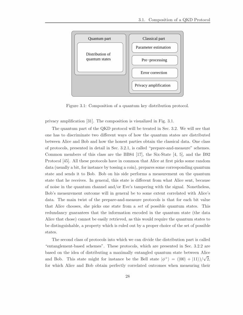
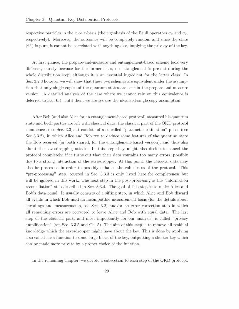
Figure 3.1: Composition of a quantum key distribution protocol.
privacy amplification [31]. The composition is visualized in Fig. 3.1.
The quantum part of the QKD protocol will be treated in Sec. 3.2. We will see that
one has to discriminate two different ways of how the quantum states are distributed
between Alice and Bob and how the honest parties obtain the classical data. One class
of protocols, presented in detail in Sec. 3.2.1, is called “prepare-and-measure” schemes.
Common members of this class are the BB84 [17], the Six-State [4, 5], and the B92
Protocol [45]. All these protocols have in common that Alice at first picks some random
data (usually a bit, for instance by tossing a coin), prepares some corresponding quantum
state and sends it to Bob. Bob on his side performs a measurement on the quantum
state that he receives. In general, this state is different from what Alice sent, because
of noise in the quantum channel and/or Eve’s tampering with the signal. Nonetheless,
Bob’s measurement outcome will in general be to some extent correlated with Alice’s
data. The main twist of the prepare-and-measure protocols is that for each bit value
that Alice chooses, she picks one state from a set of possible quantum states. This
redundancy guarantees that the information encoded in the quantum state (the data
Alice that chose) cannot be easily retrieved, as this would require the quantum states to
be distinguishable, a property which is ruled out by a proper choice of the set of possible
states.
The second class of protocols into which we can divide the distribution part is called
“entanglement-based schemes”. These protocols, which are presented in Sec. 3.2.2 are
based on the idea of distributing a maximally entangled quantum state between Alice
and Bob. This state might for instance be the Bell state |φ+〉 = (|00〉 + |11〉)/√
2,
for which Alice and Bob obtain perfectly correlated outcomes when measuring their
28
Chapter 3. Quantum Key Distribution Protocols
respective particles in the x or z-basis (the eigenbasis of the Pauli operators σx and σz,
respectively). Moreover, the outcomes will be completely random and since the state
|φ+〉 is pure, it cannot be correlated with anything else, implying the privacy of the key.
At first glance, the prepare-and-measure and entanglement-based scheme look very
different, mostly because for the former class, no entanglement is present during the
whole distribution step, although it is an essential ingredient for the latter class. In
Sec. 3.2.3 however we will show that these two schemes are equivalent under the assump-
tion that only single copies of the quantum states are sent in the prepare-and-measure
version. A detailed analysis of the case where we cannot rely on this equivalence is
deferred to Sec. 6.4; until then, we always use the idealized single-copy assumption.
After Bob (and also Alice for an entanglement-based protocol) measured his quantum
state and both parties are left with classical data, the classical part of the QKD protocol
commences (see Sec. 3.3). It consists of a so-called “parameter estimation” phase (see
Sec 3.3.2), in which Alice and Bob try to deduce some features of the quantum state
the Bob received (or both shared, for the entanglement-based version), and thus also
about the eavesdropping attack. In this step they might also decide to cancel the
protocol completely, if it turns out that their data contains too many errors, possibly
due to a strong interaction of the eavesdropper. At this point, the classical data may
also be processed in order to possibly enhance the robustness of the protocol. This
“pre-processing” step, covered in Sec. 3.3.3 is only listed here for completeness but
will be ignored in this work. The next step in the post-processing is the “information
reconciliation” step described in Sec. 3.3.4. The goal of this step is to make Alice and
Bob’s data equal. It usually consists of a sifting step, in which Alice and Bob discard
all events in which Bob used an incompatible measurement basis (for the details about
encodings and measurements, see Sec. 3.2) and/or an error correction step in which
all remaining errors are corrected to leave Alice and Bob with equal data. The last
step of the classical part, and most importantly for our analysis, is called “privacy
amplification” (see Sec. 3.3.5 and Ch. 5). The aim of this step is to remove all residual
knowledge which the eavesdropper might have about the key. This is done by applying
a so-called hash function to some large block of the key, outputting a shorter key which
can be made more private by a proper choice of the function.
In the remaining chapter, we devote a subsection to each step of the QKD protocol.
29
3.2. Quantum Part/Distribution of Quantum States
3.2 Quantum Part/Distribution of Quantum States
In this section we present a general description of the distribution step of a QKD proto-
col. The next two subsections treat the prepare-and-measure variant (see Sec. 3.2.1) and
the entanglement-based variant (see Sec. 3.2.2) separately. Their equivalence is proven
in the third subsection, Sec. 3.2.3.
Although most QKD implementations only encode bits into quantum states, we will
generalize our analysis to arbitrary alphabets of size d. Note that in the end, after
the classical post-processing (cf. Sec. 3.3), we will always end up with a key that only
consists of bits. Let |φjx〉, with x = 0, 1, . . . , d − 1 and j = 1, 2, . . . , r be a family
a pure states such that for each j, the |φjx〉 are linearly independent. Furthermore, let
Mj = M jx,M
j? denote some set of POVMs such that Mj unambiguously discriminates
the |φjx〉, i.e. 〈φj
x|M jy |φj
x〉 ∼ δxy for all j. Again for completeness, we include the
possibility of inconclusive outcomes, represented by M j? , in the case where the |φj
x〉 are
not mutually orthogonal. However, the inconclusive outcomes will not play any special
role in our analysis. We say that the index j labels the encoding of the dit x and
the states |φjx〉 are called signal states. Finally, let PJ and PK be some probability
distributions on the set of encodings 1, 2, . . . , r. The probability distribution PJ will
be used by Alice to choose an encoding for each signal, and likewise PK will be used by
Bob to choose a POVM Mk. For the sake of completeness, define a third probability
distribution PX on 0, 1, . . . , d − 1 for the choice of the dit x that is to be encoded.
Although in our analysis we will only consider uniform distributions, i.e. PX(x) = 1/d
for all x, for the sake of generality and in order to unify the notation, we allow also for
arbitrary probability distributions PX .
The idea behind the introduction of additional redundancy by having r different
encodings (that is, dr different quantum states are used to encode only one dit) is that
it becomes more difficult to identify a certain state taken from a set of different states
as the size of the set increases. However, if the encoding j is known, Mj is constructed
such that this task is feasible.4
3.2.1 Prepare-and-measure Schemes
Most QKD protocols fall into this category, for instance the BB84 [17], Six-State [4],
and the B92 [45] Protocol. They all have in common that Alice encodes some classical
4In a real experiment, even the implementation of a measurement that discriminates only two (non-
orthogonal) states might not be highly efficient [46]. However, in our analysis we will ignore such
practical problems.
30
Chapter 3. Quantum Key Distribution Protocols
information (e.g., a bit) into a set of quantum states that are sent to Bob. Bob on his
part will measure the quantum system and obtains some classical measurement result.
We will now discuss the details of this procedure.
Alice chooses n numbers xi ∈ 0, 1, . . . , d − 1 and n numbers ji ∈ 1, 2, . . . , raccording to PX and PJ , respectively, prepares the state |φj1
x1〉 ⊗ · · · ⊗ |φjn
xn〉, and
sends it to Bob.
Since Alice keeps her choice of all dits and encodings in mind, the combined state
describing her classical data and the prepared quantum system is given by
ρnJAB =
d−1∑
x=0
r∑
j=1
PJ(j)PX (x)|j〉〈j| ⊗ |x〉〈x| ⊗ |φjx〉〈φj
x|
⊗n
(3.1)
Consider for a moment that Alice and Bob are connected by a noiseless channel (i.e.,
there is no eavesdropper), thus Bob receives[∑d−1
x=0
∑rj=1 PJ(j)PX (x)|φj
x〉〈φjx|]⊗n
undis-
turbed. In order to “decode” the x’s, he chooses n numbers ki ∈ 1, 2, . . . , r according
to PK and performs the POVM Mk1 ⊗ · · · ⊗ Mkn on this state obtaining the result
y ∈ 0, 1, . . . , d − 1, ?×n. That is, for each signal arriving, he picks a encoding ki ac-
cording to the probability distribution PK and performs a measurement, given by Mki
on the quantum state. He adds the outcome yi to a list which forms his “raw key”.
Again, there might be inconclusive measurement outcomes depending on the specific
protocol.5
To fill this sketch of a protocol with life, let us consider a common version of the BB84
protocol: In the BB84 protocol, we have r = 2 different encodings for a bit (d = 2),
namely the eigenstates of the σz and σx Pauli operators, i.e. |φ10〉 = |0〉, |φ1
1〉 = |1〉,|φ2
0〉 = (|0〉 + |1〉)/√
2, and |φ21〉 = (|0〉 − |1〉)/
√2. Since for each encoding, the two
different “codewords” are orthogonal, the two POVMs employed by Bob are given by
Mj = |φj0〉〈φ
j0|, |φ
j1〉〈φ
j1|, j = 1, 2, without inconclusive outcomes. The bits 0 and 1
will be encoded with equal probability, therefore we choose PX to be a flat distribution.
On the other hand, it turns out that it is preferable that Alice almost always uses the
same encoding to increase the efficiency of the protocol [47]. Bob on his side takes PK
to be flat again, that is, he randomly chooses M1 or M2 for his measurement.
5Note that we do not take into account any inconclusive outcomes which originate from experimental
imperfections such as dark counts, stray light, detector dead time, or losses.
31
3.2. Quantum Part/Distribution of Quantum States
3.2.2 Entanglement-based Schemes
In contrast to the class of protocols described in the previous section, entanglement-
based protocols aim at distributing a maximally entangled state between Alice and Bob.
The correlation inherent in this state and its detachment from the environment enable
Alice and Bob to create a common secret key. This is achieved in the following way:
Suppose Alice and Bob share the maximally entangled state |φ+〉 = (|00〉 + |11〉)/√
2
and measure their respective system in the computational basis. They will both obtain
either the bit 0 or 1 with probability 1/2. Moreover, since |φ+〉 is pure, it can easily
be shown that no other (classical or quantum) system can contain any information
about this bit [28, 27]. This leaves one with the problem of how to distribute the
state |φ+〉, since it has to be prepared locally and therefore it has to pass through the
quantum channel which potentially can be attacked by the eavesdropper. The original
idea [19, 27] was to let Alice prepare n copies of |φ+〉, send the second half to Bob,
resulting in a state ρ⊗n of n non-maximally entangled states ρ. Instead of performing
classical privacy amplification on their data, Alice and Bob now run an entanglement
distillation protocol [25, 48, 49] on all these copies and obtain a number m < n of
maximally entangled states. Unfortunately, such a protocol is hard to implement because
it requires quantum memory. However, it has been shown [28] that the entanglement
distillation can equivalently be performed using certain quantum error-correcting codes
(CSS codes [29, 30]). We do not need to go into the details here, since we only consider
classical privacy amplification.
The distribution of quantum states using an entanglement-based protocols works as
follows:
Alice chooses n numbers ji ∈ 1, 2, . . . , r according to PJ , prepares the state∑d−1
x=0
√
PX(x)|x〉|φj1x 〉 ⊗ · · · ⊗∑d−1
x=0
√
PX(x)|x〉|φjn
x 〉, and sends the second half
(the |φji
x 〉 part for all i) to Bob.
The only difference to the prepare-and-measure scheme is that each signal is in a coherent
superposition of |x〉|φjx〉 for all x. The encoding j of each signal is chosen classically,
thus the combined state describing Alice’s data and the quantum systems sent to Bob
is given by
ρJAB =
r∑
j=1
PJ(j)|j〉〈j| ⊗(
d−1∑
x=0
√
PX(x)|x〉|φjx〉)(
d−1∑
x=0
√
PX(x)〈x|〈φjx|)
⊗n
(3.2)
The “encoding” is performed by Alice measuring each of her quantum states in the
computational basis |x〉, resulting in a measurement outcome xi with probability
32
Chapter 3. Quantum Key Distribution Protocols
PX(xi). The decoding step works in the same way as for the prepare-and-measure
version: Bob chooses n numbers ki ∈ 1, 2, . . . , r according to PK and performs the
POVM Mk1 ⊗ · · · ⊗Mkn on this state. He obtains the result y ∈ 0, 1, . . . , d− 1, ?×n,
which again might contain inconclusive measurement outcomes.
3.2.3 Equivalence of Entanglement-based and Prepare-and-measure
Schemes
It is easy to see that the schemes presented in previous two subsections are equivalent,
that is, they provide Alice and Bob with the same correlations and are indistinguishable.
We see that any prepare-and-measure scheme can be recast entanglement-based by
introducing a purifying system in the state (3.1). We say that a quantum state ρ ∈ B(H)
is purified [50, 51] by a state σ ∈ B(Haux) (or by a system Haux) if there exists a pure
state |Ψ〉 ∈ H⊗Haux such that ρ and σ are both marginal states of this pure state, i.e.
ρ = trHaux|Ψ〉〈Ψ| and σ = trH |Ψ〉〈Ψ| (see also Sec. 4.4). Here, we choose the system R
such that it purifies the mixture∑d−1
x=0 PX(x)|x〉〈x| ⊗ |φjx〉〈φj
x| and is neither controlled
by Alice and Bob nor by Eve:
ρJABR =
r∑
j=1
PJ (j)|j〉〈j| ⊗(
d−1∑
x=0
√
PX(x)|x〉|φjx〉|x〉R
)(d−1∑
x=0
√
PX(x)〈x|〈φjx|〈x|R
)
⊗n
(3.3)
This state is equal to the state (3.2) from Alice’s, Bob’s, and Eve’s point of view, thus the
prepare-and-measure scheme is contained in the class of entanglement-based schemes.
Conversely, consider the state (3.2) describing an entanglement-based scheme. If
Alice measures the system A in the |x〉-basis without revealing the result, we arrive
at the state (3.1). This shows that any entanglement-based scheme is also contained in
the class of prepare-and-measure schemes, which proofs their equivalence.
In certain cases however one would like to go further and describe a protocol as
being entirely based on distributing entangled states. To this end, define the so-called
encoding operators
Aj =
d−1∑
x=0
|φjx〉〈x|. (3.4)
For simplicity, let us assume that the |φjx〉 are mutually orthogonal for each encoding j,
implying that the Aj are unitary.
Using these operators, we see that the signal states can be prepared by the action
33
3.2. Quantum Part/Distribution of Quantum States
of Aj :d−1∑
x=0
√
PX(x)|x〉|φjx〉 = 1⊗Aj
d−1∑
x=0
√
PX(x)|x〉|x〉 =: 1⊗Aj |φ+〉, (3.5)
where we have defined |φ+〉 =∑d−1
x=0
√
PX(x)|x〉|x〉, which, for PX(x) = 1/d is equal to
the maximally entangled state in d dimensions. In this way, the preparation (encoding)
can be absorbed into the operator Aj. Suppose that we can find some operators Aj such
that 1 ⊗ Aj |φ+〉 = Aj ⊗ 1|φ+〉 holds. This means that Alice can perform a modified
encoding operation Aj on her half of the state |φ+〉 instead of applying Aj to Bob’s part.
In particular, the distributed state is now simply |φ+〉, independent of the encoding
and thus it is the same for each protocol. It is easy to see that we can always [1]
choose Aj := AjT if Aj does not map the states |x〉 from Cd into a higher-dimensional
Hilbert space. The important case where this happens is when Alice sends (probably
unintentionally) more than one copy of the signal states, that is Aj =∑d−1
x=0 |φjx〉
⊗n〈x|for some n > 1. The analysis of these multi-photon events is more involved and will be
discussed for the example of the “Tomographic Protocol” in Sec. 6.4. Until then, we
will stick to case where n = 1 and where the encoding maps states from Cd to Cd′ with
d′ ≤ d.
3.2.4 Eavesdropping
An important consequence of this modified encoding approach in which for any protocol
only one particular state |φ+〉 =∑d−1
x=0
√
PX(x)|x〉|x〉 has to be distributed is the simple
analysis of the eavesdropping attack: We will see in Ch. 4 that Eve’s attack can be fully
described by a unitary operation that she applies on the quantum state sent from Alice
to Bob and a “probe system” that she attaches to it. This means that the total state
shared between Alice, Bob, and Eve right after her attack is given by
|Ψ〉ABE = 1A ⊗ UBE |φ+〉AB|0〉E , (3.6)
where UBE is the unitary operation the eavesdropper applies on the system B and her
probe system E, which is in some arbitrary initial state |0〉. Eve keeps a subsystem
of BE and forwards the remaining part to Bob. Without loss of generality, we can
assume that she keeps her original probe E and sends B on to Bob, because the unitary
operation UBE can in particular contain a swapping operation of arbitrary subspaces.
This means that Bob will receive the state ρB = trAE(UBE |φ+〉〈φ+| ⊗ |0〉〈0|EU†BE),
whereas the knowledge of the eavesdropper about the key at this point is also fully
characterized by the quantum state held by her, which is
ρE = trAB(UBE |φ+〉〈φ+| ⊗ |0〉〈0|EU†BE). (3.7)
34
Chapter 3. Quantum Key Distribution Protocols
This state is independent of the particular encoding and thus, independent of the specific
protocol.
To conclude this section, we have shown that the entanglement-based and prepare-
and-measure type of the preparation of the quantum system are equivalent, in the sense
that the total states (3.1) describing the distributed quantum states together with any
classical data the honest parties hold are the same from Alice’s, Bob’s, and Eve’s point
of view. Additionally, for a restricted set of encodings, where the signals states live
in a Hilbert space of dimension not greater than d, where d is defined by the state
|φ+〉 =∑d−1
x=0
√
PX(x)|x〉|x〉, the quantum state held by the adversary is independent
of the encoding, as shown by (3.7). In particular, this holds for the BB84, B92, and
Ekert protocol. This is important because one step of the security analysis, classifying
the state held by the adversary, is therefore common for all such protocols (cf. Sec.4.3).
3.3 Classical Part
In this part of the key distribution the classical strings which Alice and Bob obtain
upon measuring the quantum state distributed in the quantum part, will be made equal
and secure. The states given in Eq. (3.1) (for the prepare-and-measure scheme) and
Eq. (3.2) (for the entanglement-based scheme) describe the situation before the signal
states reach Bob. Since they pass through a quantum channel about which Alice and
Bob have only partial knowledge (they might know some of its basic properties such as
attenuation in the absence of an eavesdropper), the state shared by Alice and Bob after
the transmission might be of a complicated structure. In general, it is only possible
for Alice and Bob to obtain some partial knowledge about this state, because there
are many states that are compatible with a given measurement statistics. In Ch. 6 we
present a special protocol in which Alice and Bob can in principle exactly infer which
quantum state they shared prior to the measurement. In this section, we present the
classical part of the protocol by only assuming that Alice and Bob share some n-partite
state ρnAB .
3.3.1 Measurement
We already indicated in Sec. 3.2.1 and 3.2.2 how Bob decodes the dit string chosen
by Alice: For the ith signal, he chooses an encoding ki according to the probability
distribution PK , applies the POVM Mki and obtains the outcome yi ∈ 0, 1, . . . , d−1, ?,where “?” denotes an inconclusive answer.
Denote by x = (x1, x2, . . . , xn) the dit string Alice has chosen in the preparation step
35
3.3. Classical Part
(or which she has measured in an entanglement-based scheme). Since each xi was chosen
according to the probability distribution PX , we can introduce a random variable X with
range of all n dit-strings 0, 1, . . . , d−1×n and an associated probability distribution PX
with PX(x) = PX(x1) · · ·PX(xn). Likewise, let y with yi ∈ 0, 1, . . . , d−1, ? denote the
n outcomes of Bob’s application of Mk. Finally, we can introduce random variables Y,
J, and K for Bob’s measurement outcomes and Alice’s and Bob’s choice of the encoding,
respectively.
3.3.2 Parameter Estimation
All data Alice and Bob gathered is described by the random variables X, Y, J, and K.
By comparing (part of) this data, Alice and Bob can try to infer some characteristics of
the eavesdropping attack. In particular, they have to be able to conclude whether it is
at least possible to create a secret key from those classical data. An important quantity
that can be estimated in this step is the quantum bit error rate (QBER), which is the
fraction of signals i for which Alice and Bob chose the same encoding, i.e. ji = ki, but
where Bob got a measurement outcome different from what Alice prepared, i.e. xi 6= yi.
The calculation of secret key rates (cf. Sec. 6.2) also yields results that are dependent
on the parameters Alice and Bob estimate in this step.
3.3.3 Pre-processing
It might be advantageous for Alice and Bob not to generate a secret key directly from
X and Y, but to have Alice calculate two new random variables U and V obtained by
some conditional probability distributions PU|X and PV|U. Alice keeps U and sends V
to Bob. (Bob will calculate a guess for U using V, the error correction information, and
his data Y, see below.) In our analysis, we will neglect this step, thus choosing U ≡ X
and V to be trivial (uniform). Nevertheless, it turned out that the performance of a
protocol can actually be improved by choosing U to be a “noisy” version of X. On the
other hand, the variable V does not seem to play any role [1].
3.3.4 Information Reconciliation
Up to this point, the classical strings x and y Alice and Bob hold are not identical,
because in general, they originate from measuring some quantum state which is disturbed
due to Eve’s interaction. In the information reconciliation step, the strings are made
equal. To achieve this, Alice sends error correction information — quantified by another
random variable W — to Bob, who uses Y, V, W to calculate a guess for U. (In our
36
Chapter 3. Quantum Key Distribution Protocols
case, U ≡ X, since we neglect the pre-processing.) We assume that after this step, Alice
and Bob hold the same random variable U, at least with probability 1−ε. Usually, in this
step W contains at least the information about J, that is, which encodings Alice used
for each signal. A simple so-called “sifting” method for Bob is then to simply discard all
signals for which he used a different encoding. There exist also more sophisticated sifting
strategies, for instance in the SARG protocol [52], in which more signals get discarded,
but Eve also has less knowledge about the remaining ones. In addition to the sifting,
also all other errors that were introduced by Eve or the noisy channel are corrected.
Since we neglect the pre-processing step, we will from now on denote the dit string
shared by Alice and Bob (from which the key will be created) by X and the error
correction information sent by Alice by W, which is also known by Eve, because it is
sent over the public channel. It has been shown in [53] that the minimal amount of
information W which allows Bob to guess X with probability of at least 1− ε, knowing
only Y and W , is given by Hε0(X|Y ). This quantity, called conditional smooth Renyi
entropy, will be discussed in detail in Sec. 5.3 (see also Sec. 5.2).
3.3.5 Privacy Amplification.
Although at this point Alice and Bob share a common dit string x, it is not very
reasonable to directly use it as a secret key, since the eavesdropper might have too much
information about it. In the privacy amplification step, Alice and Bob shrink the length
of the key x and at the same time reduce the information that Eve might have about
it, thereby generating a secret key. Since privacy amplification is an important step
which will be the starting point of the analysis of of secret key rates, we review this
sub-protocol in more detail in Sec. 5.2. We also review the security analysis of privacy
amplification and present an expression for an achievable secret key length, as found
in [1].
37

3.3. Classical Part
38
Chapter 4
Security of Quantum Key
Distribution
In this section, we present methods that enable us to quantify the secrecy of a key
created with a QKD protocol described in the previous chapter. The main peculiarity
is that we want to quantify the knowledge that an adversary holding a quantum system
might have about a classical key. For a better understanding of this issue, we start with
a brief review of a classical security definition in Sec. 4.1 and show that generalizing the
classical definition for the quantum case does not yield a satisfactory security definition.
In the main section of this chapter, Sec. 4.2, we will see how this issue can be settled by
a completely different approach, involving the distance of quantum states.
4.1 Security in the Classical World
Before focusing on the problem of how to define the security of a QKD protocol, we
take one step back and consider the classical case. Suppose Alice and Bob run some
(classical) key distribution protocol such that, at the end, they hold two strings SA
and SB, respectively. We now ask ourselves what qualifies SA and SB as secret key?
Certainly, the answer to that question depends on “how secure” we want the key to be.
Usually, we are interested in a security definition which is not based on any assumptions
such as limited computing power or memory, or restricting the possible actions of the
eavesdropper. Rather, we are looking for a statement that qualifies a key as information-
theoretically secure: [54]
Definition 4.1.1. Let SA, SB, and Z be random variables and ε ≥ 0. Then (SA, SB) is
an ε-secure key pair with respect to Z if there exists some random variable S with range
39
4.2. Security in the Quantum World
S such that
Prob[SA = SB = S] ≥ 1 − ε (4.1)
H(S) = log |S| (4.2)
I(S : Z) ≤ ε. (4.3)
This definition has the following intuitive interpretation: The strings SA and SB
are secure with respect to an adversary having access to the information contained in1
Z, if they are almost (except with probability ε) equal to a uniform string S about
which the eavesdropper has almost no information. Uniformity is quantified by the
Shannon information H(S), and the knowledge of the eavesdropper about Z is given
by the mutual information I(S : Z). It is important to allow for small deviations from
the case of a perfectly secure key (ε = 0), since perfect security is impossible to obtain
with a probabilistic protocol running on a finite time scale. Def. 4.1.1 already provides
us with the strongest security definition appropriate for any classical application, thus
it seems reasonable to take it as a starting point for our quantum version.
Let us now think about how we can translate our consideration from the last sub-
section to the quantum world: Clearly, at the end of any (quantum) protocol, Alice and
Bob are left with classical data, the key. However, we have to consider the case that the
adversary conducts an attack that provides her with a quantum system which contains
some information about the key (we will see in the next section how she can do this).
In this case, a natural generalization of Eq. (4.3) would be to bound Eve’s accessible
information, which is the maximal amount of information she can obtain about the key
when choosing the optimal measurement on her quantum state. However, it has been
shown that such an approach is problematic, due to an undesirable feature of the ac-
cessible information: Although the adversary’s accessible information about the key S
is negligibly small, it might happen that S is completely insecure in certain applica-
tions [55]. This shows that the security definition Def. 4.1.1 and also its generalization
is not appropriate in the quantum case. In the next section, we introduce a security
definition which accurately describes secret keys generated with QKD protocols.
4.2 Security in the Quantum World
As we have already mentioned, in quantum key distribution we need to deal with the
case in which the adversary potentially holds a quantum system correlated with the
1For instance, Z might describe all public communication the adversary learns.
40
Chapter 4. Security of Quantum Key Distribution
classical data to which the privacy amplification is to be applied. Moreover, we need
to keep in mind that a QKD protocol is a probabilistic procedure that needs to be
described at least partly by classical probability theory. For instance, we have to be
able to include in the right way cases where the eavesdropper is extraordinarily lucky
when it comes to making decisions such as the choice of measurement bases. In every
protocol it might happen that Eve by accident chooses all the time the right basis in an
intercept-resend attack, but obviously only with exceedingly small probability. A second
major issue which one has to deal with when looking for reasonable security definitions
for QKD is universal composability : Certainly, the key generated by a QKD scheme
will be used in some other cryptographic application (e.g. a one-time pad); quite rarely,
Alice and Bob will be satisfied with shared randomness. Therefore, we need to consider
a QKD protocol composed with another cryptographic primitive. In this section, we will
introduce a security definition that takes this into account.
In order to describe such universal composability, we need a formalism introduced
in [56], the so-called “cq-states” defined in Def. 2.2.2: Consider a protocol together with
an arbitrary eavesdropping strategy that can output keys from some set X . For instance,
if the protocol consists of n rounds each creating a single bit, X might be the set of all
n-bit strings. Suppose a key x ∈ X is generated with probability px, and in this case
the eavesdropper holds a quantum system ρxE. Introducing a classical random variable
X with range X and probability distribution PX(x) := px, the state
ρXE =∑
x∈X
PX(x)|x〉〈x| ⊗ ρxE, (4.4)
describes all possible outcomes of the QKD protocol, together with the corresponding
states of the adversary. Using this formalism, we can introduce the following definition
of a secret key [37, 55, 57, 58]:
Definition 4.2.1. Let ρSASBE ∈ B(HS ⊗ HS ⊗ HE) be a ccq-state for some random
variables SA and SB with range S and let ε ≥ 0. We say that (SA, SB) is an ε-secure
key pair, if
‖ρSASBE − ρuniform ⊗ ρE‖ ≤ ε, (4.5)
where ρuniform =∑
s∈S |s〉〈s| ⊗ |s〉〈s|/|S| is the state describing an identical, uniformly
distributed key pair, and ρE = trSA,SB(ρSASBE).
The interpretation of the state ρSASBE is that Alice and Bob hold (not necessarily
identical) bit strings described by the random variables SA and SB, respectively, and
Eve holds a quantum system ρE that might be correlated with them. The ideal case, in
which Alice’s and Bob’s strings are identical and uniformly distributed, together with
41
4.3. Classification of Eavesdropping Strategies
Eve being completely uncorrelated with them, is given by ρuniform ⊗ ρE . A distance of ε
of the state ρSASBE to this ideal scenario means that the key pair (SA, SB) behaves as
an ideal key, except with probability ε.
4.3 Classification of Eavesdropping Strategies
In this section, we will give a classification of eavesdropping strategies based on the
complexity of the eavesdropper’s interaction with the quantum states and measure-
ment. Formally, the set of all possible eavesdropping strategies can be divided into
three classes, “individual”, “collective”, and “coherent” attacks. Individual attacks are
the simplest ones, corresponding to an eavesdropper with little power. Coherent attacks
are potentially the most powerful, assuming an eavesdropper with unlimited technolog-
ical power and resources, only being limited by the laws of nature. More concretely,
these classes of strategies are defined by how Eve interacts with the quantum signals
that are sent from Alice to Bob and how she processes the information she gathers in
this way. The most general way to describe how information about a quantum system
ρA is extracted is the following: Attach an ancilla system in a predefined state |0〉〈0|E to
ρA and perform a unitary operation U on the composite system ρA ⊗ |0〉〈0|E. Then do
a measurement on the ancilla system ρE := trA(U †ρA ⊗ |0〉〈0|EU). The measurement is
given by a POVM M = Mj which yields outcome j with probability tr(Mjρ), when
measuring a state ρ. We denote the classical probability distribution which is obtained
in this way by P ρM, i.e. P ρ
M(j) = tr(Mjρ).
Consider the case where Alice sends n quantum systems ρ1A, . . . , ρ
nA to Bob. An indi-
vidual attack is an attack where Eve attaches an ancilla system |0〉〈0|E to each state ρiA,
applies the same unitary operation U and measures her part of all the composite systems
individually using a POVM M1 for each system. Collective attacks are more general
concerning the measurement, as they allow the eavesdropper to measure all ancilla sys-
tems collectively, using a POVM Mn acting on all of her probes simultaneously. The
most general attack is the coherent attack, in which it is assumed that Eve attaches one
“large” ancilla system to the total state ρ1A⊗· · ·⊗ρn
A and then performs a global unitary
transformation Un and measurement. More formally, the probability distribution that
the eavesdropper obtains for each class of attacks is given by:
Individual: Pρ1
E
M1 · · ·Pρn
E
M1 , ρiE = trA(U †ρi
A ⊗ |0〉〈0|EU), (4.6)
Collective: Pρ1
E⊗···⊗ρn
E
Mn , ρiE = trA(U †ρi
A ⊗ |0〉〈0|EU), (4.7)
Coherent: P ρE
Mn , ρE = trA(U †n(ρ1
A ⊗ · · · ⊗ ρnA) ⊗ |0〉〈0|EUn), (4.8)
42
Chapter 4. Security of Quantum Key Distribution
Note that in this classification we always included a final measurement on the eavesdrop-
per’s system. This assumption has to some extent only a historical legitimation, since
before the introduction of universal composability, the mutual information was used to
quantify the eavesdropper’s knowledge about the key. Thus, one had to classify how the
adversary extract classical information out of her quantum state, which naturally leads
to the distinction we have presented so far.
In the previous section we have seen that if we demand universal composable security,
we have to consider the case where the adversary keeps a quantum system beyond the
end of the QKD protocol. Since the distinction between individual and collective attacks
is only on the level of measurements, for our security analysis which does not consider
measurements on the adversary’s system, these attacks are actually equivalent. The
only two possibilities we can now discriminate is whether Eve’s attaches a probe to each
signal individually (the collective attack) or globally to all signals (the coherent attack).
4.4 The Role of Purifications
This section covers a simple mathematical concept in quantum information theory, pu-
rifications. Note that there exists two different notions of the word “purification”: One
of them describes the process of performing a global operation on several identical copies
of input states, such that the purity of some of them is increased. One example of this
process in entanglement distillation. When we are talking about a purification of some
state ρ ∈ B(H), we mean a pure state |Ψ〉 ∈ H⊗Haux from a higher-dimensional Hilbert
space such that traux |Ψ〉〈Ψ| = ρ. In subsection 4.4.1, we explain how this concept can
be used to find the quantum state describing the system of Alice, Bob, and Eve. Sub-
section 4.4.2 deals with physical processes that create purifications. This section partly
goes beyond the concepts of QKD, but we believe that the results are interesting on
their own.
4.4.1 Purifications in QKD
In chapter 5 dealing with privacy amplification, it is shown that it is important for the
analysis of the protocol to know the overall distributed state ρABE describing Alice’s,
Bob’s and Eve’s system after the eavesdropping attack, but before the measurements.
We have already derived in Sec. 3.2.3 that this state is given by
|Ψ〉ABE = UBE(1⊗Aj |φ+〉)|0〉E , (4.9)
43
4.4. The Role of Purifications
where the encoding operators Aj account for the signal states used in the protocol and
|φ+〉 =∑d−1
x=0
√
PX(x)|x〉|x〉. Eq. (4.9) is valid for all three classes of eavesdropping
strategies presented in the previous section, but for simplicity, we investigate it for
collective attacks. Also recall that for the idealized scenario in which in fact single
copies of the signal states |φjx〉 are prepared, the preparation can be performed by the
action of some modified encoding operators Aj acting on Alice’s system,
|Ψ〉ABE = Aj ⊗ UBE |φ+〉|0〉E, (4.10)
thus the attack of the eavesdropper is performed on (one half of) the state |φ+〉, in-
dependently of the actual encoding. However, Eq. (4.10) is not of great help, because
it still contains an arbitrary (unknown) unitary operation UBE . Fortunately, one can
easily characterize Eve’s state simply in terms of the state shared between Alice and
Bob after the distribution, ρAB. This is because if Eve applies a unitary operation on
the pure state |φ+〉 sent by Alice, UBE |φ+〉|0〉E = |Ψ〉ABE , the overall state |Ψ〉ABE will
remain pure and fulfills trE |Ψ〉〈Ψ|E = ρAB , i.e., Eve holds the purifying system of ρAB .
This approach is particularly suited for the analysis of the tomographic protocol
(cf. Ch. 6) as in this protocol it is (at least in principle) possible for Alice and Bob
to determine the state ρAB they share after the distribution. As we will see, for the
calculation of the achievable key rate it is necessary to know the quantum state Eve
holds, which then can be easily calculated by assuming that Eve holds the purifying
system of ρAB.
4.4.2 On the (Im)possibility of Physical Purification
The question that arises in this context is: “How realistic is the assumption that Eve
can create a purification of a given quantum system?” Being realistic means that there
should exist a physical process, mapping the input state to its purification. We started
investigating this topic in view of its application to QKD, as it is presented in the pre-
vious section. Specifically, we ask whether it is possible to purify a number of unknown
quantum states by a single physical operation. However, it turned out that in QKD,
this question can be answered by “no”.
For any state ρ ∈ B(H), from the spectral decomposition ρ =∑
i pi|λi〉〈λi|, with
pi ≥ 0 and∑
i pi = 1, a purification is given by |Ψ〉 =∑
i
√pi|λi〉|χi〉, where the |χi〉 are
mutually orthogonal states in an auxiliary Hilbert space Haux. Such a state is unique
up to unitary operation on Haux [51]. Since we are interested in physical processes, we
look for completely positive and trace preserving maps Λ (which we will call “purifier”)
fulfilling tr Λ(ρ)2 = 1 (purity) and traux Λ(ρ) = ρ (“faithfullness”).
44
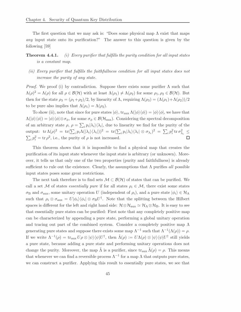
Chapter 4. Security of Quantum Key Distribution
The first question that we may ask is: “Does some physical map Λ exist that maps
any input state onto its purification?” The answer to this question is given by the
following [59]
Theorem 4.4.1. (i) Every purifier that fulfills the purity condition for all input states
is a constant map.
(ii) Every purifier that fulfills the faithfullness condition for all input states does not
increase the purity of any state.
Proof. We proof (i) by contradiction. Suppose there exists some purifier Λ such that
Λ(ρ)2 = Λ(ρ) for all ρ ∈ B(H) with at least Λ(ρ1) 6= Λ(ρ2) for some ρ1, ρ2 ∈ B(H). But
then for the state ρ3 = (ρ1+ρ2)/2, by linearity of Λ, requiring Λ(ρ3) = (Λ(ρ1)+Λ(ρ2))/2
to be pure also implies that Λ(ρ1) = Λ(ρ2).
To show (ii), note that since for pure states |φ〉, traux Λ(|φ〉〈φ|) = |φ〉〈φ|, we have that
Λ(|φ〉〈φ|) = |φ〉〈φ|⊗σφ, for some σφ ∈ B(Haux). Considering the spectral decomposition
of an arbitrary state ρ, ρ =∑
i pi|λi〉〈λi|, due to linearity we find for the purity of the
output: tr Λ(ρ)2 = tr(∑
i piΛ(|λi〉〈λi|))2 = tr(∑
i pi|λi〉〈λi| ⊗ σλi)2 =
∑
i p2i trσ2
λi≤
∑
i p2i = tr ρ2, i.e., the purity of ρ is not increased.
This theorem shows that it is impossible to find a physical map that creates the
purification of its input state whenever the input state is arbitrary (or unknown). More-
over, it tells us that only one of the two properties (purity and faithfullness) is already
sufficient to rule out the existence. Clearly, the assumptions that Λ purifies all possible
input states poses some great restrictions.
The next task therefore is to find sets M ⊂ B(H) of states that can be purified. We
call a set M of states essentially pure if for all states ρi ∈ M, there exist some states
σB and σaux, some unitary operation U (independent of ρi), and a pure state |φi〉 ∈ HA
such that ρi ⊗ σaux = U |φi〉〈φi| ⊗ σBU†. Note that the splitting between the Hilbert
spaces is different for the left and right hand side: H⊗Haux ≃ HA⊗HB. It is easy to see
that essentially pure states can be purified: First note that any completely positive map
can be characterized by appending a pure state, performing a global unitary operation
and tracing out part of the combined system. Consider a completely positive map Λ
generating pure states and suppose there exists some map Λ−1 such that Λ−1(Λ(ρ)) = ρ.
If we write Λ−1(ρ) = traux Uρ ⊗ |ψ〉〈ψ|U †, then Λ(ρ) := UΛ(ρ) ⊗ |ψ〉〈ψ|U † still yields
a pure state, because adding a pure state and performing unitary operations does not
change the purity. Moreover, the map Λ is a purifier, since traux Λ(ρ) = ρ. This means
that whenever we can find a reversible process Λ−1 for a map Λ that outputs pure states,
we can construct a purifier. Applying this result to essentially pure states, we see that
45
4.4. The Role of Purifications
we have a map Λ(ρi) = trB Uρi ⊗ σauxU† that maps each state ρi ∈ M to a pure state
|φi〉. Additionally, there exists a reverse map Λ−1(|φi〉〈φi|) = traux U†|φi〉〈φi| ⊗ σBU
which implies that there exists a purifier for the set M.
Not so obvious, essentially pure state are the only states that can be collectively
purified by a single physical operation. This is formalized by the following [59]
Theorem 4.4.2. Let M ⊂ B(H). Then the following statements are equivalent:
(i) M is a set of essentially pure states.
(ii) A purifier for M exists.
(iii) There exists a completely positive and trace preserving map Λ such that tr Λ(ρ)2 =
1 for all ρ ∈ M and ‖ρ− ρ′‖ = ‖Λ(ρ) − Λ(ρ′)‖ for all ρ, ρ′ ∈ M.
Proof. For the proof, see [59].
Although this theorem classifies all states that can be purified completely, it is in
general not easy to check whether a set of states is essentially pure.
Let us close our excursion about physical purification with the remark that, al-
though the impetus for the study of this topic was the description of eavesdropping
attacks in QKD, the concept presented in this section is not directly applicable: For
the entanglement-based scheme (cf. Sec. 3.2.2), Eve seeks to create a purification of
the state ρAB that gets distributed between Alice and Bob. Since Alice sends half of
the state |φ+〉AB =∑d−1
x=0
√
PX(x)|x〉|x〉, Eve can only act on this half of the state:
|φ+〉 → 1A ⊗ UBE |φ+〉AB |0〉E =: |Ψ〉ABE . Thus obviously, after her attack, the overall
state |Ψ〉ABE is pure and she holds the purifying system ρE = trAB |Ψ〉〈Ψ|ABE of the dis-
tributed state ρAB = trE |Ψ〉〈Ψ|ABE . On the other hand, for the prepare-and-measure
scheme (cf. Sec. 3.2.1), Alice sends one of the r signals states |φxj 〉 to Bob. But here, Eve
is not interested in obtaining a purification of each single state. Rather, she would like to
have the purifying system of the state describing all possible signals, Eq. (3.1). But we
already have shown in Sec. 3.2.3 that this state is equivalent to the entanglement-based
version, therefore we know that Eve can actually obtain the purifying system.
46
Chapter 5
Privacy Amplification
This chapter deals with the privacy amplification (PA) protocol Alice and Bob apply
after the information reconciliation step (cf. Sec. 3.3.4). We start in Sec. 5.1 by ex-
plaining the basic ideas of privacy amplification from a purely classical point of view.
Although in QKD, PA remains a classical protocol, i.e. it is some algorithm which is
applied to classical data. Problems arise when we need to consider the case where the
adversary holds a quantum system which might be correlated with this data. In Sec. 5.2,
we will deal with this issue. The main result which we present in this section was derived
in [37, 1]; it is an expression for the maximally achievable key length one can obtained
by privacy amplification, as a function of entropies of the quantum states the adversary
holds. These entropies are discussed in detail in Sec. 5.3, because they play a crucial role
in the calculation of the key length. This section will be a cornerstone for the analysis
of the “Tomographic Protocol” in Ch. 6.
5.1 Introduction
The aim of privacy amplification is to turn a string of (e.g.) bits held by the honest par-
ties and about which the adversary might have some knowledge into a secret one. This is
in general done by applying a certain function which shrinks the length of the string, but
on the other hand outputs a key about which Eve has less information. In this section,
we present a classical scenario as an example of how this can be achieved. We denote
the string that Alice and Bob hold by random variables X and Y, respectively, with
range X = Y = 0, 1n. Eve’s knowledge is quantified by a random variable Z with the
same range, and their correlation is given by a tripartite probability distribution PXYZ.
For simplicity, we assume that the data is generated by independent and identically per-
formed experiments, that is, the probability distribution PXYZ factorizes with respect
47
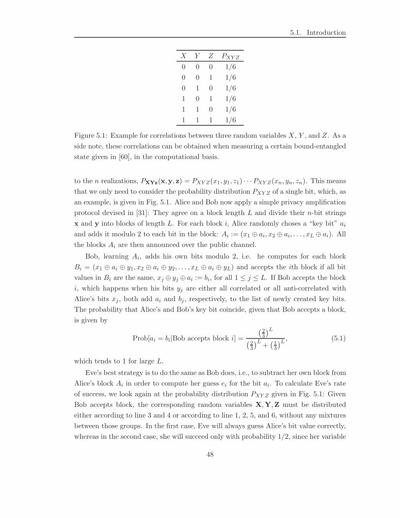
5.1. Introduction
X Y Z PXY Z
0 0 0 1/6
0 0 1 1/6
0 1 0 1/6
1 0 1 1/6
1 1 0 1/6
1 1 1 1/6
Figure 5.1: Example for correlations between three random variables X, Y , and Z. As a
side note, these correlations can be obtained when measuring a certain bound-entangled
state given in [60], in the computational basis.
to the n realizations, PXYz(x,y, z) = PXY Z(x1, y1, z1) · · ·PXY Z(xn, yn, zn). This means
that we only need to consider the probability distribution PXY Z of a single bit, which, as
an example, is given in Fig. 5.1. Alice and Bob now apply a simple privacy amplification
protocol devised in [31]: They agree on a block length L and divide their n-bit strings
x and y into blocks of length L. For each block i, Alice randomly choses a “key bit” ai
and adds it modulo 2 to each bit in the block: Ai := (x1 ⊕ ai, x2 ⊕ ai, . . . , xL ⊕ ai). All
the blocks Ai are then announced over the public channel.
Bob, learning Ai, adds his own bits modulo 2, i.e. he computes for each block
Bi = (x1 ⊕ ai ⊕ y1, x2 ⊕ ai ⊕ y2, . . . , xL ⊕ ai ⊕ yL) and accepts the ith block if all bit
values in Bi are the same, xj ⊕ yj ⊕ ai := bi, for all 1 ≤ j ≤ L. If Bob accepts the block
i, which happens when his bits yj are either all correlated or all anti-correlated with
Alice’s bits xj , both add ai and bj, respectively, to the list of newly created key bits.
The probability that Alice’s and Bob’s key bit coincide, given that Bob accepts a block,
is given by
Prob[ai = bi|Bob accepts block i] =
(23
)L
(23
)L+(
13
)L, (5.1)
which tends to 1 for large L.
Eve’s best strategy is to do the same as Bob does, i.e., to subtract her own block from
Alice’s block Ai in order to compute her guess ei for the bit ai. To calculate Eve’s rate
of success, we look again at the probability distribution PXY Z given in Fig. 5.1: Given
Bob accepts block, the corresponding random variables X,Y,Z must be distributed
either according to line 3 and 4 or according to line 1, 2, 5, and 6, without any mixtures
between those groups. In the first case, Eve will always guess Alice’s bit value correctly,
whereas in the second case, she will succeed only with probability 1/2, since her variable
48
Chapter 5. Privacy Amplification
is completely uncorrelated from Alice’s in that situation. Thus,
Prob[ai = ei|Bob accepts block i] =
(13
)L+(
23
)L 12
(23
)L+(
13
)L, (5.2)
which tends to 1/2 for large L. This means that in the limit of large block length, Alice
and Bob can generate a new pair of strings (ai, bi), which are almost perfectly correlated,
yet completely unknown to Eve.
This simple privacy amplification scheme may no be very efficient, since possibly
very large block lengths L are needed to remove Eve’s correlations with the key. We will
focus on another method, the so-called two-universal hashing. Roughly speaking, Alice
randomly chooses a function f from a certain set of functions (see Def. 5.1.1 below) and
computes f(x). Then she announces f via the public channel to Bob, who on his side
computes f(y). The key pair is then given by (f(x), f(y)), which can be shown to be
more private than the original data (x,y) before. We will formalize this for the relevant
quantum mechanical case in Sec. 5.2.
Definition 5.1.1. A family of two-universal functions is a set F of functions F : X → Ytogether with a probability distribution PF , such that
Prob[f(x) = f(x′)] ≤ 1
|Y| , ∀x 6= x′ ∈ X , (5.3)
where f ∈ F is randomly chosen according to PF .
We are interested in hash functions, i.e., functions where the cardinality of the image
is (much) smaller than that of the domain. In particular, we will consider functions
mapping their input to a bit string, that is, F : X → 0, 1ℓ, with ℓ ≤ |X |. In the
following, we will call ℓ the key length.
5.2 Privacy Amplification in the Quantum World
The main peculiarity with which we need to deal is the fact that the eavesdropper holds
a quantum system which is correlated with Alice’s and Bob’s data. This implies that we
cannot argue in the way we did in the previous section, and we have also explained in
Sec. 4.1 that it is not enough to consider arbitrary measurements for Eve. It is important
that we consider that the adversary holds a quantum system throughout the protocol.
In this section, we review a result showing that privacy amplification by two-universal
hashing can generate unconditionally secure keys. At first, we focus on the case where
Alice’s and Bob’s data are already identical. Afterwards, we will loosen this assumption
by including the error correction step into the analysis.
49
5.2. Privacy Amplification in the Quantum World
Assume that Alice and Bob apply the privacy amplification protocol at a step in
which Alice’s and Bob’s classical data is already identical. Therefore, we only need
to consider a single random variable X which is correlated with a quantum system E
under Eve’s control, as described by a cq-state ρXE . Alice chooses a hash function f
from the set F according to PF (which may be taken to be uniform), computes f(x),
and communicates f to Bob. After this step, they hold a classical bit string f(x), where
x is chosen according to PX and f according to PF . Since the choice of f is broadcasted
over the classical channel, we have to add this information to Eve’s pool of knowledge.
We denote the quantum state describing this situation together with the system E that
was correlated with x by ρF (X)EF . Formally, it is given by
ρF (X)EF =∑
f∈F
PF (f)ρf(X)E ⊗ |f〉〈f |, (5.4)
where ρf(X)E is the joint state where a particular function f is applied to X:
ρf(X)E =∑
x∈X
|f(x)〉〈f(x)| ⊗ ρxE (5.5)
Note that in (5.4), both the system E and F are under Eve’s control.
The following theorem bounds the distance of a secret key generated by two-universal
hashing from an ideal key:
Theorem 5.2.1. Let ρXE ∈ B(HX ⊗ HE) be a cq-state for some random variable X
with range X and let F : X → 0, 1ℓ be a family of two-universal hash functions.
Furthermore, denote by ρF (X)EF the state after the two-universal hashing. Then
‖ρF (X)EF − ρU ⊗ ρEF‖ ≤ 1
22−
1
2(S2(ρXE)−S0(ρE)−ℓ), (5.6)
where ρU = 1/2ℓ∑
x∈0,1ℓ |x〉〈x| is a uniform key and ρEF = trF (X) ρF (X)EF and ρE =
trX ρXE.
Proof. For the proof, see [37, 58].
The quantities S2 and S0, occurring in (5.6) (and Sε′2 and Sε′
0 that appear below
in (5.7)) are called (smooth) Renyi entropies. We devote Sec. 5.3 to their detailed
analysis. It turns out that the bound in (5.6) can be generalized and potentially improved
by exploiting the triangle inequality of the trace distance. The simple calculation can
be found in [58], yielding
‖ρF (X)EF − ρU ⊗ ρEF‖ ≤ 1
22−
1
2(Sε
′
2 (ρXE)−Sε′
0 (ρE)−ℓ) + 2ε′, (5.7)
50
Chapter 5. Privacy Amplification
for any ε′ ≥ 0.
When studying QKD protocols, one is usually interested in the achievable key length
for a given scenario. Moreover, one might require that the generated key fulfills some
security requirements, for instance, it is ε-secure for some predefined ε. Thus, one would
like to have the left-hand side of (5.7) to be upper bounded by ε, i.e.
1
22−
1
2(Sε
′
2 (ρXE)−Sε′
0 (ρE)−ℓ) + 2ε′!≤ ε. (5.8)
This relation holds if the secret key length ℓ is bounded by
ℓ ≤ Sε′2 (ρXE) − Sε′
0 (ρE) + 2 log(2ε− 4ε′). (5.9)
In this equation, we have one free parameter 0 ≤ ε′ < ε/2, with ε fixed by the security
requirement. In [37], ε′ was put to ε/4, for no apparent reason. To keep our notation
consistent with [1], we start with a slightly modified version of (5.9), which was used
in [1], however no proof was given:
ℓ ≤ Sε′2 (ρXE) − Sε′
0 (ρE) + 2 log(ε). (5.10)
with ε′ = (ε/8)2 (again for no apparent reason).
Relation (5.10) has the following interpretation: If Alice and Bob managed to dis-
tribute some random string X about which the adversary has some knowledge (in the
form of a correlated quantum state), such that the total system is described by the state
ρXE , then, performing a PA protocol based on two-universal hashing, it is impossible
to turn X into ε-secret of length ℓ larger than the right hand side of Eq. (5.10). Note
that this result is independent of how Alice and Bob actually obtained X, in particular,
which distribution protocol they chose (cf. Sec. 3.2). Another very important feature of
relation (5.10) is that the bound on the key length ℓ is tight, i.e. for an optimal choice
of the PA protocol, equality can be achieved [61]. Since the proof of this statement is
even constructive [61], we will from now on assume that Alice and Bob use an optimal
PA protocol, thus, we will take
ℓ = Sε′
2 (ρXE) − Sε′
0 (ρE) + 2 log(ε), (5.11)
where ℓ is the maximally achievable key length, as a starting point for our further
analysis (cf. also [1]).
Note that up to now, we have assumed that Alice and Bob both already hold the
same string X. However to achieve this, they have to correct their original strings X and
Y (cf. Sec. 3.3.4). This involves sending some error correction information W over the
51
5.3. Smooth Renyi Entropies
public channel, which means that some information is leaking to Eve. One can show [1]
that, using an optimal error correction protocol1, the length of W is given by Hε′0 (X|Y).
Here, Hε′0 is another smooth Renyi entropy, which is defined below in Sec. 5.3. This
amount has to be subtracted from (5.11), leading to [1]
ℓ = Sε′
2 (ρXE) − Sε′
0 (ρE) −Hε0(X|Y) + 2 log(ε). (5.12)
Finally, we have obtained an expression for the obtainable secret key length ℓ for the
case where Alice and Bob start with some classical data X and Y, respectively, and
where the correlation between the data X and the eavesdropper is described by the
quantum state ρXE .
5.3 Smooth Renyi Entropies
In this section, we derive technical results concerning smooth Renyi entropies. Part
of these result can be found in [62]. We start with the general definition and show in
Sec. 5.3.2 how it can be reformulated in way that allows us to explicitly calculate the
entropies for arbitrary input states. The main focus will lie on the analysis of Sε2, S
ε0,
and Hε0 , which are the entropies occurring in the formula for the key length, Eq. (5.12).
For these cases, we derive in Sec. 5.3.3 a solution which can be calculated by a simple
algorithm. This allows us to calculate the obtainable key rate for the “Tomographic
Protocol” (cf. Ch. 6). Finally, in Sec. 5.3.4, we derive some additivity properties of the
Renyi entropies Sε2 and Sε
0, which play an important role in the analysis of multi-photon
events in Sec. 6.4.
5.3.1 General Properties
Before we give the definition of the smooth Renyi entropies, we have to introduce some
notation: Recall that we denote by P(Cd) the set of positive operators acting on Cd and
by B(Cd) := σ ∈ P(Cd) : trσ = 1 the set of all density matrices acting on Cd. For
ρd ∈ B(Cd), define ed′(ρd) := ρd⊕diag (0, . . . , 0)︸ ︷︷ ︸
d′−d
to be an embedding of ρd into a Hilbert
space of dimension d′. Finally, let Bε(ρd) := σd′ ∈ B(Cd′) : d′ ≥ d, ‖σd′ − ed′(ρd)‖ ≤ εbe the set of density operators of dimension greater than or equal to d which are ε-close
to ρd. In this chapter, we will often index a density matrix with the dimension of the
Hilbert space on which it is acting.
1Note that realistic error correction protocols need more overhead. Their analysis however is much
more involved and a topic of current research on its own.
52
Chapter 5. Privacy Amplification
The quantum version of smooth Renyi entropies is defined in the following way [1, 37]
Definition 5.3.1. Let ρd ∈ B(Cd), α ∈ [0,∞], and ε ∈ [0,∞). The ε-smooth Renyi
entropy of order α of ρd is defined as
Sεα(ρd) :=
1
1 − αinf
σd′∈Bε(ρd)
log trσαd′ . (5.13)
For the definition of the classical conditional smooth Renyi entropy, we use the nota-
tion that for some random variable X with range X and associated probability distribu-
tion PX , we denote by Bε(PX) := QX : QX(x) ≤ PX(x)∀x ∈ X ,∑x∈X QX(x) ≥ 1− εthe set of probability distributions QX which are ε-close to PX .
Definition 5.3.2. Let X and Y be two random variables with range X and Y, respec-
tively, and let PXY be some joint probability distribution. Furthermore, let α ∈ [0,∞],
and ε ∈ [0,∞). The conditional ε-smooth Renyi entropy of order α of X given Y is
defined as
Hεα(X|Y ) :=
1
1 − αinf
QXY ∈Bε(PXY )maxy∈Y
log∑
x∈X
QX|Y =y(x)α. (5.14)
We are in particular interested in the entropies occurring in Eq. (5.12), that is, Sε2,
Sε0, and Hε
0 . For these cases, the two definitions from above reduce to the following
form:
Sε2(ρd) = − inf
σd′∈Bε(ρd)
log trσ2d′ (5.15)
Sε0(ρd) = inf
σd′∈Bε(ρd)
log rankσd′ (5.16)
Hε0(X|Y ) = min
A:Prob[A]≥1−ε
(
maxy∈Y
log |x ∈ X : PXA|Y =y(x) > 0|)
, (5.17)
where the minimum in (5.17) ranges over all events A occurring with probability of at
least 1 − ε.
The explicit calculation of these entropies will be done in Sec. 5.3.3. However,
for the case of the quantum Renyi entropies Sε2 and Sε
0, we will first translate the
minimization over the set Bε(ρd) to a minimization over real vectors, which eases the
analysis significantly. The derivation of this transformation is the subject of the following
section.
5.3.2 Simplifications for Sε2 and Sε
0
The main result of this section is that since the Renyi entropies only depend on the
eigenvalues of the states taken from the set Bε(ρd), the minimization can equivalently
53
5.3. Smooth Renyi Entropies
be performed over the set of spectra that can be found in Bε(ρd). This statement is
proven below in Lemma 5.3.1.
Recall the definition of the set of operators which are ε-close to a given one, Bε(ρd) :=
σd′ ∈ B(Cd′) : d′ ≥ d, ‖σd′ − ed′(ρd)‖ ≤ ε. Now define Dε(ρd) := σd′ ∈ Bε(ρd) :
[σd′ , ed′(ρd)] = 0 to be the set of all such operators which additionally commute with
ρd. Finally, let λ(ρd) be the ordered spectrum of ρd, i.e. λ(ρd) = (λ1, . . . , λd) ∈ Rd in
ascending order and denote by ‖λ−λ′‖ = 1/2∑
i |λi − λ′i| the distance of the vectors λ
and λ′.
Lemma 5.3.1. The two sets ΛεB(ρd) = λ(σd′) : σd′ ∈ Bε(ρd), and Λε
D(ρd) = λ(σd′) :
σd′ ∈ Dε(ρd), defined as the sets of spectra that correspond to the sets of density matrices
Bε(ρd) and Dε(ρd), respectively, are identical.
Proof. Since Dε(ρd) ⊂ Bε(ρd), it follows directly that ΛεD(ρd) ⊂ Λε
B(ρd). To show the
other inclusion, let µ ∈ ΛεB(ρd). This means that there exists some σd′ ∈ Bε(ρd) such
that µ = λ(σd′) and ‖σd′ − ed′(ρd)‖ ≤ ε. From the spectral decomposition ed′(ρd) =∑d′
i=1 νi|i〉〈i| define σd′ :=∑d′
i=1 µi|i〉〈i|, i.e. [σd′ , ed′(ρd)] = 0. We then have that
‖σd′ − ed′(ρd)‖ = ‖λ(σd′) − λ(ed′(ρd))‖ (5.18)
= ‖λ(σd′) − λ(ed′(ρd))‖ (5.19)
≤ ‖σd′ − ed′(ρd)‖ (5.20)
≤ ε, (5.21)
which implies that σd′ ∈ Dε(ρd), and since µ = λ(σd′), it follows that µ ∈ ΛεD(ρd).
We will now reformulate the definition of Dε(ρd). Since for all σd′ ∈ Dε(ρd), we
have that [σd′ , ed′(ρd)] = 0, it follows that σd′ = σd ⊕ σd′−d with σd, σd′−d ∈ P(Cd) and
trσd, tr σd′−d ≤ 1. Thus,
‖σd′ − ed′(ρd)‖ = ‖σd − ρd‖ + ‖σd′−d‖ (5.22)
= ‖σd − ρd‖ +1
2trσd′−d (5.23)
= ‖σd − ρd‖ +1
2(1 − trσd). (5.24)
We can therefore write
Dε(ρd) = σd ⊕ σd′−d ∈ B(Cd′) : (5.25)
trσd, trσd′−d ≤ 1, [σd, ρd] = 0, ‖σd − ρd‖ ≤ ε− 1
2(1 − trσd). (5.26)
54
Chapter 5. Privacy Amplification
Turning to the smooth Renyi entropies Sεα(ρd), since they only depend on the eigenvalues
of ρd, we can use the above lemma to replace the infimum over the set Bε(ρd) by the
infimum over Dε(ρd):
Sεα(ρd) :=
1
1 − αinf
σd′∈Bε(ρd)
log trσαd′ (5.27)
=1
1 − αinf
σd′∈Dε(ρd)
log trσαd′ (5.28)
=1
1 − αinf
σd⊕σd′−d
∈Dε(ρd)log tr(σd ⊕ σd′−d)
α (5.29)
=1
1 − αinf
σd⊕σd′−d
∈Dε(ρd)log(trσα
d + trσαd′−d) (5.30)
=1
1 − αinf
σd∈Dε(ρd),d′≥dlog
[
trσαd + (d′ − d)
(1 − trσd
d′ − d
)α]
(5.31)
=1
1 − αinf
σd∈Dε(ρd),d′≥dlog
[
trσαd +
1
(d′ − d)α−1(1 − trσd)
α
]
(5.32)
=1
1 − αinf
σd∈Dε(ρd)log tr σα
d , α 6= 1 (5.33)
The crucial step in this derivation is from (5.30) to (5.31): Note that σd′−d is only
restricted by trσd′−d = 1− trσd, otherwise, it is completely arbitrary (it only has to be
positive). Thus the infimum over trσαd′−d can be evaluated separately, and it is obtained
for a uniform distribution of the eigenvalues, i.e. each eigenvalue is trσd′−d/(d′ − d) =
(1− tr σd)/(d′ − d). The only freedom one still has is to choose the dimension d′ and σd,
which is now taken from the set
Dε(ρd) := σd ∈ P(Cd) : trσd ≤ 1, [σd, ρd] = 0, ‖σd − ρd‖ ≤ ε− 1
2(1 − trσd), (5.34)
which is loosely speaking the “remaining” part of the set Dε(ρd) when forgetting about
σd′−d. Concerning the step from (5.32) to (5.33), note that the second term in the
logarithm is always non-negative, so for α > 1 the infimum is obtained for d′ → ∞,
whereas for α < 1 it is obtained for d′ = d, which leads to (5.33) in both cases. In
particular, for α < 1, the final infimum has to be taken over all σd ∈ Dε(ρd) with
tr σd = 1. Since for α < 1, the minimization is performed over the set Dε(ρd) containing
states with arbitrary trace, we can split up the infimum by fixing the trace to be t and
finally minimizing over t, which leads to
Sεα(ρd) =
11−α inf
σd∈Dε1(ρd)
log trσαd for α < 1
11−α inf
1−ε≤t≤1inf
σd∈Dεt(ρd)
log trσαd for α > 1
, (5.35)
55
5.3. Smooth Renyi Entropies
where we have defined the set Dεt (ρd) to be the set Dε(ρd) where all density matrices
have trace t:
Dεt (ρd) := σd ∈ P(Cd) : trσd = t, [σd, ρd] = 0, ‖σd − ρd‖ ≤ ε− 1
2(1 − t) (5.36)
The range of the parameter t is obtained by using the following lower bound on the
trace distance of the operators σd and ρd which occurs in (5.36):
ε− 1
2(1 − t) ≥ ‖σd − ρd‖ (5.37)
=1
2tr |σd − ρd| (5.38)
≥ 1
2| tr(σd − ρd)| (5.39)
=1
2(1 − t) (5.40)
⇔ t ≥ 1 − ε, (5.41)
where we have used that σd and ρd commute.
The calculations can finally be further simplified by observing that the function
which is to be minimized, log trσαd , only depends on the eigenvalues of σd. Since the
infimum in (5.33) only ranges over all σd taken from a set Dε(ρ) of operators which
commute with the input state ρ, we can entirely focus on the eigenvalues of ρ (this is
the essence of Lem. 5.3.1). Therefore, we can write
Sεα(ρd) =
11−α inf
µ∈Λε
D1(ρd)
logd∑
i=1µα
i for α < 1
11−α inf
1−ε≤t≤1inf
µ∈Λε
Dt(ρd)
logd∑
i=1µα
i for α > 1
(5.42)
where
ΛεDt
(ρd) = µ ∈ Rd :
d∑
i=1
µi = t, ‖µ − λ(ρd)‖ ≤ ε− 1
2(1 − t). (5.43)
To conclude, we have transformed the minimization over a subset of a Hilbert space
to a minimization over a set of real vectors subjected to simple constraints. In the next
subsection, we will evaluate Eq. (5.42) for two special cases (namely α = 0 and α = 2)
which play an important role in the privacy amplification step (cf. Sec. 5.2).
5.3.3 Explicit Calculation of Sε2, Sε
0, and Hε0
The aim of this section is to construct an algorithm that computes the Renyi entropies
Sε2 and Sε
0. Due to the minimization involved, it is not possible to present a closed
expression, since Sεα(ρ) strongly depends on the explicit distribution of the eigenvalues
of ρ. However, we found a strategy that allows us compute these entropies efficiently.
56
Chapter 5. Privacy Amplification
Calculation of Sε0(ρ)
For the case of α = 0, from Eq. (5.42) we find that the smooth Renyi entropy takes a
very simple form:
Sε0(ρ) = inf
µ∈Λε
D1(ρ)
log
d∑
i=1
µ0i (5.44)
= infµ∈Λε
D1(ρ)
log |µi > 0|, (5.45)
where the set ΛεD1
(ρ) is defined in (5.43). Note that for α < 1, there is no optimization
over t, rather, we only need to consider the case t = 1. Calculating Sε0(ρ) is thus
equivalent to finding the solution x of the following optimization problem:
|xi > 0| → min (5.46)n∑
i=1
xi = 1 (5.47)
n∑
i=1
|xi − yi| ≤ 2ε, (5.48)
where the vector y corresponds to the vector of eigenvalues of ρd (which is given). The
solution to this optimization problem is very simple: Find the largest number k such
that the sum of the smallest k values yi is smaller or equal to ε. We define the solution
x by starting from y (which certainly satisfies (5.47) and (5.48)) and modify it in the
following way: Put the smallest k values yi to zero and rise the largest yi by ε such that
both (5.47) and (5.48) are still satisfied. The solution x obtained in this way fulfills
|xi > 0| = |yi > 0| − k.
To be more specific, let ρ ∈ B(Cd) some density matrix having eigenvalues λi with
degeneracy ni, for 1 ≤ i ≤ m, i.e.∑m
i=1 niλi = 1 and∑m
i=1 ni = d. We assume that the
λi are given in ascending order. Define
s−(r) :=r∑
i=1
niλi, (5.49)
for 0 ≤ r ≤ m, which is the sum of r smallest different eigenvalues. (For r = 0, the sum
is taken to be zero.) Moreover, let
b− := maxr : s−(r) ≤ ε (5.50)
be the largest number r such that the sum of the r smallest different eigenvalues is
smaller than ε. Then the number k we are looking for is thus given by
k =
b−∑
i=1
ni +
⌊ε− s−(b−)
λb−+1
⌋
, (5.51)
57
5.3. Smooth Renyi Entropies
where ⌊x⌋ denotes the largest integer smaller than or equal to x. Finally, we have found
that
Sε0(ρ) = log(d− k). (5.52)
Calculation of Hε0(X|Y )
The calculation of this classical Renyi entropy is similar to the calculation of Sε0(ρ)
performed in the previous section. First note that we can rewrite its definition,
Hε0(X|Y ) = min
A:Prob[A]≥1−εmaxy∈Y
log |PAy|, (5.53)
introducing the set PAy := x ∈ X : PXA|Y =y(x) > 0. In the analysis of the Tomo-
graphic Protocol (see Sec. 6.1) we will encounter the case where the set PAy is actually
independent of y. This means that we can drop the minimization over y and simply
consider the set PAy0, for some arbitrarily chosen y0. Thus the only restriction on the
size of the PAy0is given by A. The minimization over all such events occurring with
probability of at least 1 − ε can be solved in the following way: It is easy to see that
all such events are necessarily of the form [X = x1] ∨ [X = x2] ∨ · · · ∨ [X = xk] with∑k
i=1 PX(xi) ≥ 1−ε. Since we are searching for the smallest set PAy0, we are interested
in those events which are most restrictive, i.e. which have k as small as possible. This
means we need to find the smallest number k such that the sum of k largest probabil-
ities occurring in PX|Y =y0is greater than or equal to 1 − ε. We then have found that
Hε0(X|Y ) = log k.
To explicitly calculate k, consider some probability distribution PX|Y =y0having m
entries pi with multiplicity ni, for 1 ≤ i ≤ m, i.e.∑m
i=1 nipi = 1. We again assume that
the pi are given in ascending order. In analogy to the calculation of Sε0(ρ), define
s+(r) :=
r∑
i=1
nm−i+1pm−i+1, (5.54)
which is the sum of r largest different probabilities. Also define
b+ := minr : s+(r) ≥ 1 − ε (5.55)
to be the smallest number r such that sum of the largest r probabilities is greater than
or equal to 1 − ε. The number k is then given by
k =
b+∑
i=1
nm−i+1 +
⌊s+(b+) − (1 − ε)
pm−b+
⌋
, (5.56)
58
Chapter 5. Privacy Amplification
which finally leads to
Hε0(X|Y ) = log k. (5.57)
Note that this result only holds if the number of non-zero entries in PX|Y =y does not
depend on y. (However, this is the only case we are interested in.) If this is not the
case, one would first need to find the corresponding y which maximizes the number of
non-zero entries, which corresponds to evaluating the maximum in (5.53).
Calculation of Sε2(ρ)
The calculation of Sε2(ρ) is more involved, mainly because we have an additional pa-
rameter t which corresponds to the trace of the density matrices over which we have to
minimize (in contrast to the entropies Sε0 and Hε
0). From Eq. (5.42), we find that
Sε2(ρ) = − inf
1−ε≤t≤1inf
µ∈Λε
Dt(ρ)
logd∑
i=1
µ2i , (5.58)
where the set ΛεDt
(ρ) is defined by (5.43). We defer the minimization over t until the
very end. Therefore, for a fixed t, we are facing an optimization problem of the following
form:
(o1)n∑
i=1
x2i → min (5.59)
(c1)
n∑
i=1
xi = t (5.60)
(c2)
n∑
i=1
|xi − yi| ≤ 2ε− (1 − t) (5.61)
Here, the yi are the eigenvalues of ρd (which are given).
We will construct the solution of this optimization problem successively by a series
of small steps. First note that we can demand that the components in the vector y are
given in ascending order, i.e. yi ≤ yj for all i ≤ j. It is then easy to see that any solution
x can be ordered in the same way:
Lemma 5.3.2. Let x be a solution of (o1,c1,c2). Suppose there exist two indices k ≤ l
such that yk ≤ yl and xk ≥ xl. Then x = (x1, . . . , xl, . . . , xk, . . . , xn), i.e., the original
solution with xk and xl interchanged, is also a solution of (o1,c1,c2).
Proof. Obviously, we have that∑n
i=1 x2i =
∑ni=1 x
2i and
∑ni=1 xi =
∑ni=1 xi, that is, x
fulfills (o1) and (c1). It remains to show that also (c2) holds, which can be done by
verifying |xk − yk| + |xl − yl| ≥ |xl − yk| + |xk − yl| using the triangle inequality and
considering all (six) possible relations between xk, xl, yk, and yl separately.
59
5.3. Smooth Renyi Entropies
By successive application of Lemma 5.3.2 we see that any non-monotonically increas-
ing solution x can be turned into a monotonically increasing one x. The next lemma
reveals something about the structure of the solution.
Lemma 5.3.3. Let x be a solution of (o1,c1,c2), where the xi are in ascending order.
Then we can transform x in the following two ways without changing its optimality:
1. (a) Let J ⊂ [1, n] be the set2 of indices such that xj ≤ yj for all j ∈ J . Let jmin
be the smallest index in J such that xjmin< yjmin
and jmax the largest index
in J . Define
xjmin:= min(yjmin
, (xjmin+ xjmax
)/2) (5.62)
xjmax:= max(xjmax
− xjmin+ yjmax
, (xjmin+ xjmax
)/2), (5.63)
and xj = xj for all j 6= jmin, jmax.
(b) Permute the xjj∈J such that they are again in ascending order.
2. (a) Let K ⊂ [1, n] be the set of indices such that xk ≥ yk for all k ∈ K. Let
kmin be the smallest index in K and kmax be the largest index in K such that
xkmax> ykmax
. Define
xkmax:= max(ykmax
, (xkmin+ xkmax
)/2) (5.64)
xkmin:= min(xkmin
+ xkmax− ykmax
, (xkmin+ xkmax
)/2), (5.65)
and xk = xk for all k 6= kmin, kmax.
(b) Permute the xkk∈K such that they are again in ascending order.
Proof. We proof the assertion only for the first transformation, the proof for the second
one is completely analogous. Due to Lemma 5.3.2, step (b) preserves the optimality of
the solution. It remains to consider step (a), i.e., we have to show that x is a solution
of (o1,c1,c2). By construction, we have that xjmin− xjmin
= −xjmax+ xjmax
=: δ, which
implies that x fulfills (c1) and (c2). To show (o1), we directly calculate∑
j∈J
x2j =
∑
j 6=jmin,jmax
x2j + (xjmin
+ δ)2 + (xjmax− δ)2 (5.66)
=∑
j∈J
x2j + 2δ2 + 2δ(xjmin
− xjmax︸ ︷︷ ︸
=−2δ
) (5.67)
≤∑
j∈J
x2j . (5.68)
2It is easy to see that the set J is always non-empty unless ε = 0 and t = 1.
60
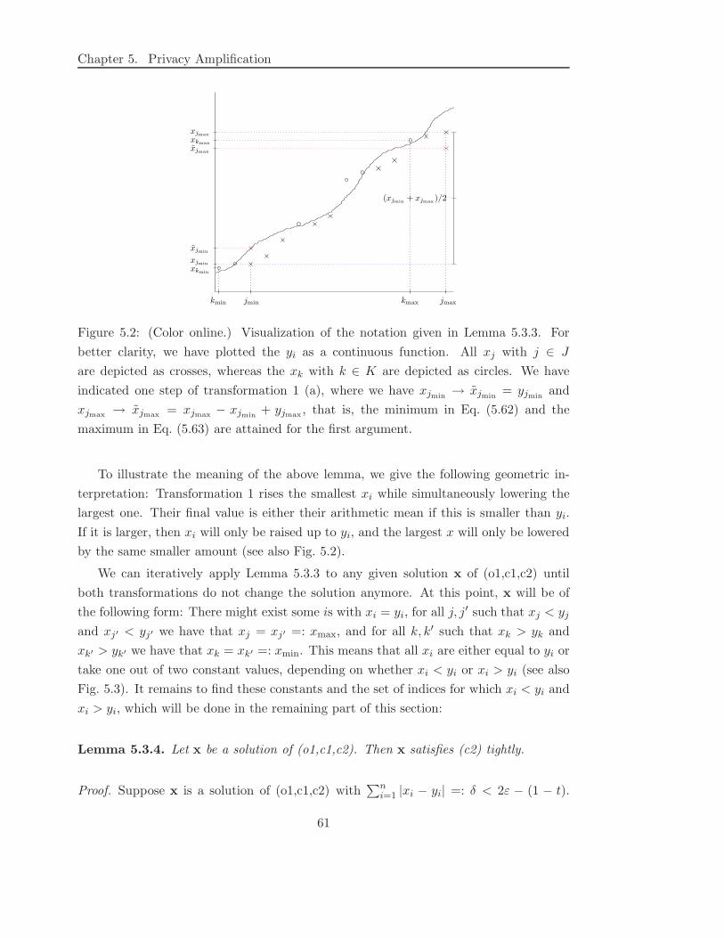
Chapter 5. Privacy Amplification
xjmax
xkmax
xjmax
xjmin
xjmin
xkmin
kmin jmin kmax jmax
(xjmin+ xjmax
)/2
Figure 5.2: (Color online.) Visualization of the notation given in Lemma 5.3.3. For
better clarity, we have plotted the yi as a continuous function. All xj with j ∈ J
are depicted as crosses, whereas the xk with k ∈ K are depicted as circles. We have
indicated one step of transformation 1 (a), where we have xjmin→ xjmin
= yjminand
xjmax→ xjmax
= xjmax− xjmin
+ yjmax, that is, the minimum in Eq. (5.62) and the
maximum in Eq. (5.63) are attained for the first argument.
To illustrate the meaning of the above lemma, we give the following geometric in-
terpretation: Transformation 1 rises the smallest xi while simultaneously lowering the
largest one. Their final value is either their arithmetic mean if this is smaller than yi.
If it is larger, then xi will only be raised up to yi, and the largest x will only be lowered
by the same smaller amount (see also Fig. 5.2).
We can iteratively apply Lemma 5.3.3 to any given solution x of (o1,c1,c2) until
both transformations do not change the solution anymore. At this point, x will be of
the following form: There might exist some is with xi = yi, for all j, j′ such that xj < yj
and xj′ < yj′ we have that xj = xj′ =: xmax, and for all k, k′ such that xk > yk and
xk′ > yk′ we have that xk = xk′ =: xmin. This means that all xi are either equal to yi or
take one out of two constant values, depending on whether xi < yi or xi > yi (see also
Fig. 5.3). It remains to find these constants and the set of indices for which xi < yi and
xi > yi, which will be done in the remaining part of this section:
Lemma 5.3.4. Let x be a solution of (o1,c1,c2). Then x satisfies (c2) tightly.
Proof. Suppose x is a solution of (o1,c1,c2) with∑n
i=1 |xi − yi| =: δ < 2ε − (1 − t).
61
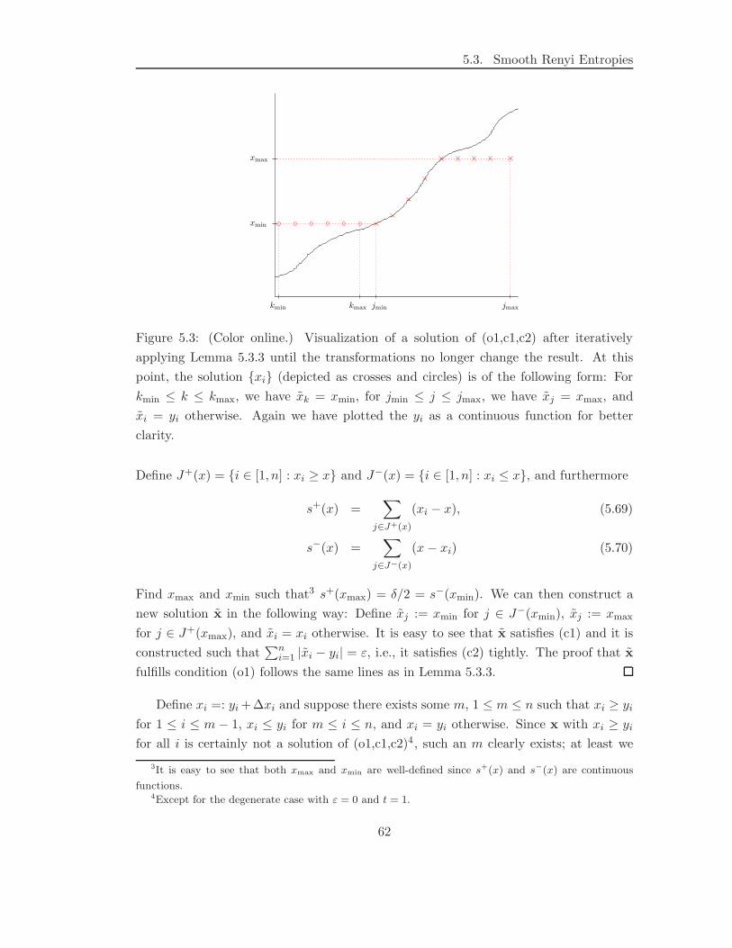
5.3. Smooth Renyi Entropies
xmin
xmax
kmin kmax jmin jmax
Figure 5.3: (Color online.) Visualization of a solution of (o1,c1,c2) after iteratively
applying Lemma 5.3.3 until the transformations no longer change the result. At this
point, the solution xi (depicted as crosses and circles) is of the following form: For
kmin ≤ k ≤ kmax, we have xk = xmin, for jmin ≤ j ≤ jmax, we have xj = xmax, and
xi = yi otherwise. Again we have plotted the yi as a continuous function for better
clarity.
Define J+(x) = i ∈ [1, n] : xi ≥ x and J−(x) = i ∈ [1, n] : xi ≤ x, and furthermore
s+(x) =∑
j∈J+(x)
(xi − x), (5.69)
s−(x) =∑
j∈J−(x)
(x− xi) (5.70)
Find xmax and xmin such that3 s+(xmax) = δ/2 = s−(xmin). We can then construct a
new solution x in the following way: Define xj := xmin for j ∈ J−(xmin), xj := xmax
for j ∈ J+(xmax), and xi = xi otherwise. It is easy to see that x satisfies (c1) and it is
constructed such that∑n
i=1 |xi − yi| = ε, i.e., it satisfies (c2) tightly. The proof that x
fulfills condition (o1) follows the same lines as in Lemma 5.3.3.
Define xi =: yi +∆xi and suppose there exists some m, 1 ≤ m ≤ n such that xi ≥ yi
for 1 ≤ i ≤ m− 1, xi ≤ yi for m ≤ i ≤ n, and xi = yi otherwise. Since x with xi ≥ yi
for all i is certainly not a solution of (o1,c1,c2)4 , such an m clearly exists; at least we
3It is easy to see that both xmax and xmin are well-defined since s+(x) and s−(x) are continuous
functions.4Except for the degenerate case with ε = 0 and t = 1.
62
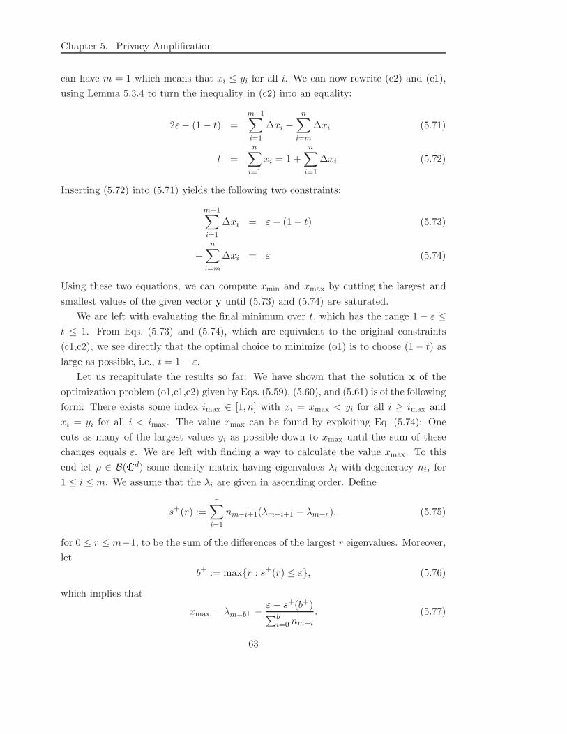
Chapter 5. Privacy Amplification
can have m = 1 which means that xi ≤ yi for all i. We can now rewrite (c2) and (c1),
using Lemma 5.3.4 to turn the inequality in (c2) into an equality:
2ε− (1 − t) =
m−1∑
i=1
∆xi −n∑
i=m
∆xi (5.71)
t =n∑
i=1
xi = 1 +n∑
i=1
∆xi (5.72)
Inserting (5.72) into (5.71) yields the following two constraints:
m−1∑
i=1
∆xi = ε− (1 − t) (5.73)
−n∑
i=m
∆xi = ε (5.74)
Using these two equations, we can compute xmin and xmax by cutting the largest and
smallest values of the given vector y until (5.73) and (5.74) are saturated.
We are left with evaluating the final minimum over t, which has the range 1 − ε ≤t ≤ 1. From Eqs. (5.73) and (5.74), which are equivalent to the original constraints
(c1,c2), we see directly that the optimal choice to minimize (o1) is to choose (1 − t) as
large as possible, i.e., t = 1 − ε.
Let us recapitulate the results so far: We have shown that the solution x of the
optimization problem (o1,c1,c2) given by Eqs. (5.59), (5.60), and (5.61) is of the following
form: There exists some index imax ∈ [1, n] with xi = xmax < yi for all i ≥ imax and
xi = yi for all i < imax. The value xmax can be found by exploiting Eq. (5.74): One
cuts as many of the largest values yi as possible down to xmax until the sum of these
changes equals ε. We are left with finding a way to calculate the value xmax. To this
end let ρ ∈ B(Cd) some density matrix having eigenvalues λi with degeneracy ni, for
1 ≤ i ≤ m. We assume that the λi are given in ascending order. Define
s+(r) :=
r∑
i=1
nm−i+1(λm−i+1 − λm−r), (5.75)
for 0 ≤ r ≤ m−1, to be the sum of the differences of the largest r eigenvalues. Moreover,
let
b+ := maxr : s+(r) ≤ ε, (5.76)
which implies that
xmax = λm−b+ − ε− s+(b+)∑b+
i=0 nm−i
. (5.77)
63
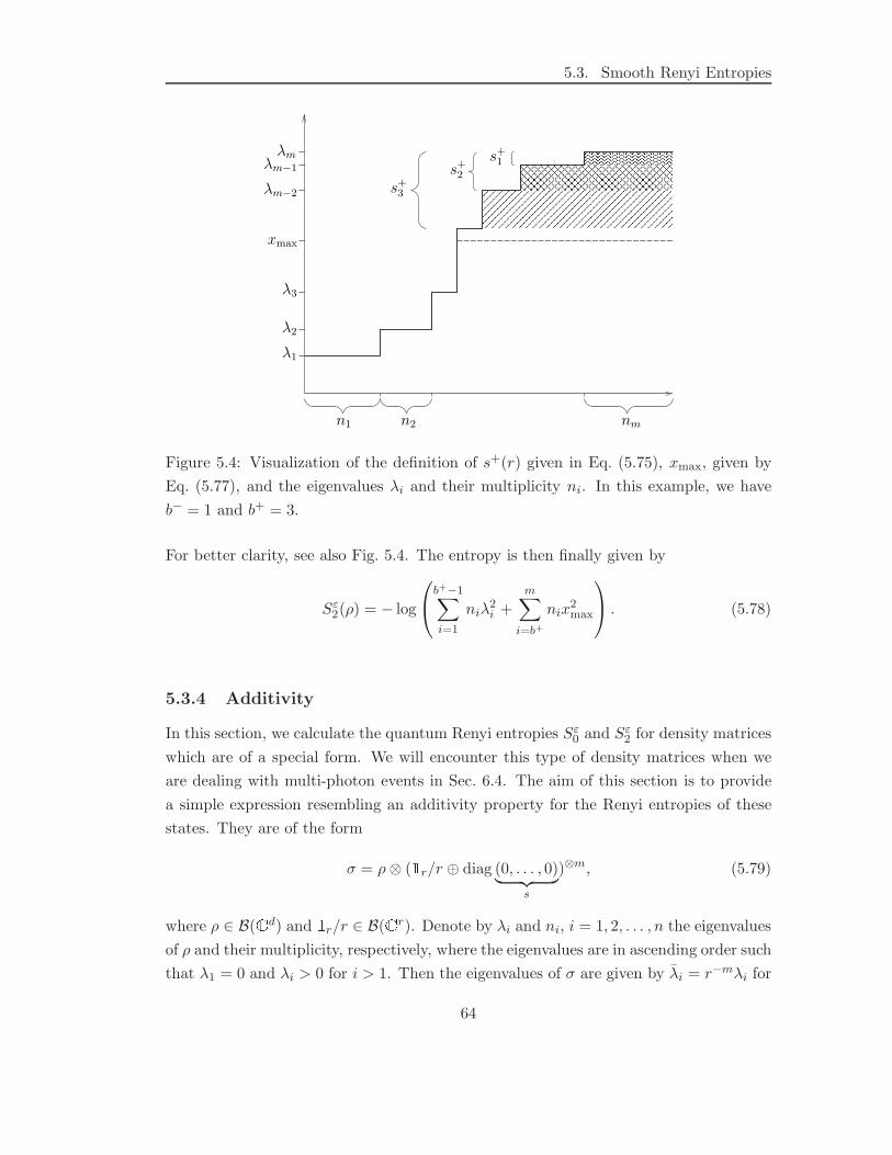
5.3. Smooth Renyi Entropies
λmλm−1
λm−2
xmax
λ3
λ2
λ1
n1 n2 nm
s+1
s+2
s+3
Figure 5.4: Visualization of the definition of s+(r) given in Eq. (5.75), xmax, given by
Eq. (5.77), and the eigenvalues λi and their multiplicity ni. In this example, we have
b− = 1 and b+ = 3.
For better clarity, see also Fig. 5.4. The entropy is then finally given by
Sε2(ρ) = − log
b+−1∑
i=1
niλ2i +
m∑
i=b+
nix2max
. (5.78)
5.3.4 Additivity
In this section, we calculate the quantum Renyi entropies Sε0 and Sε
2 for density matrices
which are of a special form. We will encounter this type of density matrices when we
are dealing with multi-photon events in Sec. 6.4. The aim of this section is to provide
a simple expression resembling an additivity property for the Renyi entropies of these
states. They are of the form
σ = ρ⊗ (1r/r ⊕ diag (0, . . . , 0)︸ ︷︷ ︸
s
)⊗m, (5.79)
where ρ ∈ B(Cd) and 1r/r ∈ B(Cr). Denote by λi and ni, i = 1, 2, . . . , n the eigenvalues
of ρ and their multiplicity, respectively, where the eigenvalues are in ascending order such
that λ1 = 0 and λi > 0 for i > 1. Then the eigenvalues of σ are given by λi = r−mλi for
64
Chapter 5. Privacy Amplification
all i, and the multiplicities are given by n1 = rmn1 + d[(r + s)m − rm)] and ni = rmni
for i > 1.
Approximate additivity of Sε0
Recall that, due to Eq. (5.52) and the proceeding discussion, Sε0(ρ) = log(dim ρ − k),
where k =∑b−
i=1 ni + ⌊(ε − s−(b−))/λb−+1⌋ with b− = maxr : s−(r) ≤ ε and s−(r) =∑r
i=1 niλi. Likewise, denote by k, b−, and s(r) all those quantities referring to σ given
by (5.79). We see that
s−(r) =
r∑
i=1
niλi =
r∑
i=2
niλi + (rmn0 + d[(r + s)m − rm]) · 0 = s−(r), (5.80)
and therefore also b− = b−. However, the expression for k is more complicated due
to the Gauss brackets involved. We introduce the quantity δ which amounts for the
rounding:
k =b−∑
i=1
ni−1 +
⌊ε− s−(b−)
λb−+1
⌋
=b−∑
i=1
ni−1 +ε− s−(b−)
λb−+1− δ (5.81)
and similar for k with δ:
k =
b−∑
i=1
ni−1 +
⌊ε− s−(b−)
λb−+1
⌋
=
b−∑
i=1
ni−1 +ε− s−(b−)
λb−+1
− δ (5.82)
Now we can express k in terms of k:
k =
b−∑
i=1
ni−i +
⌊ε− s−(b−)
λb−+1
⌋
(5.83)
=
r∑
i=2
rmni−1 + rmn0 + d[(r + s)m − rm] +
⌊ε− s−(b−)
λb−+1
⌋
(5.84)
=r∑
i=2
rmni−1 + rmn0 + d[(r + s)m − rm] +ε− s−(b−)
r−mλb−+1− δ (5.85)
= rmk + rmδ − δ + d[(r + s)m − rm]. (5.86)
Since dimσ = (r + s)m dim ρ = d(r + s)m, we finally obtain for the entropy:
Sε0(σ) = log
(d(r + s)m − rmk − d[(r + s)m − rm] − rmδ − δ
)(5.87)
= log rm + log(d− k − δ + r−mδ
)(5.88)
= log rm + log
(
(d− k)
[
1 +r−mδ − δ
d− k
])
(5.89)
= log rm + Sε0(ρ) + log
(
1 +r−mδ − δ
d− k
)
, (5.90)
65
5.3. Smooth Renyi Entropies
where the last term on the right hand side is only exponentially small in m:
log
(
1 +r−mδ − δ
d− k
)
≤ r−mδ − δ
d− k(5.91)
≤ 1
rm(d− k)(5.92)
≤ r−m for ε < 1, (5.93)
where we have used that δ < 1 and δ < 1. To conclude, for two density matrices σ and
ρ related by (5.79), we have found that
Sε0(σ) ≈ Sε
0(ρ) + log rm, (5.94)
where the approximation is up to r−m.
Exact additivity of Sε2
The general solution for Sε2 is given by Eq. (5.78): Sε
2(ρ) = − log(∑b+−1
i=1 niλ2i +∑d
i=b+ ni
x2max), with xmax = λd−b+−(ε−s+(b+))/
∑b+
i=0 nd−i, where s+(r) :=∑r
i=1 nd−i+1(λd−i+1
−λd−r) and b+ := maxr : s+(r) ≤ ε. Denote by xmax, s+(r), and b+ all these
quantities referring to σ. We now calculate
s+(r) =
r∑
i=1
nd−i+1(λd−i+1 − λd−r) (5.95)
=r∑
i=1
rmnd−i+1(r−mλd−i+1 − r−mλd−r) (5.96)
= s+(r) (5.97)
which also directly implies that b+ = b+ and xmax = r−mxmax. Finally, we find for the
entropy:
Sε2(σ) = − log
b+−1∑
i=1
niλ2i +
d∑
i=b+
nix2max
(5.98)
= − log
r−mb+−1∑
i=1
niλ2i + r−m
d∑
i=b+
nix2max
(5.99)
= Sε2(ρ) + log rm, (5.100)
which is very similar to the result obtained for Sε0, Eq. (5.94).
To conclude this section, we have shown that for density matrices of the special
form (5.79), the smooth Renyi entropies Sε0 and Sε
2 behave (for the former case at least
approximately) additive.
66
Chapter 6
Finite Key Analysis for the
Tomographic Protocol
In this chapter we present the main results of this thesis: An application of the analysis
of privacy amplification to a specific quantum key distribution protocol, the so-called
“Tomographic Protocol”. Part of the results presented here can be found in [62]. The
emphasis lies on analyzing the success of two-universal hashing for finite block sizes n.
We will not deal with any finite-size effects that may emerge from statistical issues such
as estimating an error rate in the parameter estimation step.1 Additionally we assume
that the adversary performs a collective eavesdropping attack (cf. Ch 4.3).2 Our goal
is to calculate the maximally achievable key rate of this protocol, that is the fraction
of signals (after the sifting step) that make it into the final key. This number is of
interest because of two reasons: First, it can be viewed as a measure of the efficiency
of the privacy amplification step, and second Alice and Bob can use this information to
determine how “much” privacy amplification they need to apply, because the key rate
is equal to the factor by which the raw key needs to be shrunken in order to have the
desired security.
Besides the dependence on the block size n, we present a detailed analysis of the
dependence of the key rate on a number of different parameters: We show that for a
security parameter ε (which is the probability that the key is insecure) of to 10−28, one
can still create a secret key. Moreover, we will see that the dependence on ε becomes
less pronounced as the block size n increases, which means that one can create keys with
1We will also assume that optimal error correction protocols are employed.2Is has been shown in [63] that the analysis of collective attacks is sufficient, since the most general
attacks, coherent attacks, are not more powerful, at least in the limiting case of n → ∞. Note however
that we are explicitly avoiding this approximation.
67
6.1. Description of the Protocol
higher security by increasing the block size. We are also able to compare variants of
the Tomographic Protocol using different alphabet sizes (and quantum systems of cor-
responding dimension) and show for instance that for higher error rates, low dimensions
are always favorable.
The first part of our analysis will deal with the ideal case in which Alice sends a
single copy of each signal state to Bob, as she would do if she possessed a single-photon
source. We will first derive all results for this scenario and then show in the second part
how one can include also the case where Alice sends (accidentally) more than one copy
of each state into the analysis. This is the situation one naturally encounters in most
experimental implementations.
This chapter is organized as follows: The specifics of the Tomographic Protocol are
presented in Sec. 6.1 and in Sec. 6.2 we derive the maximally achievable key rates for this
protocol, using the results from Ch. 5, at first for the idealized case where in the quantum
part of the protocol only single copies of the signal states are prepared (Sec. 6.3). This
assumption will be loosened in Sec. 6.4, where we generalize the analysis to incorporate
multi-photon events.
6.1 Description of the Protocol
The Tomographic Protocol was originally introduced in [2] (see also [3]). It is based on
the Six-State Protocol [4] and generalizations thereof to higher dimensions. The main
twist of the Tomographic Protocol is its special strategy to do parameter estimation:
Since the measurements involved in the six state protocol form a tomographically com-
plete POVM, it is (at least in principle) possible to reconstruct the density matrix of
the measured state. Alice and Bob then use this knowledge to rigorously abort the
protocol if they learn that the quantum state they shared is not compatible with some
channel model (the depolarizing channel) they are expecting. In this way, they force
the adversary to launch an attack that provides Alice and Bob with the same quantum
state as they would obtain if they were only connected by a depolarizing channel, i.e.
Eve has to perform a symmetric attack.
Such a symmetric attack has the advantage that the analysis of the privacy amplifi-
cation step becomes simple, since the density matrices involved have only a few different
eigenvalues (due to the high symmetry).
In more detail, the protocol works as follows: Alice and Bob use an alphabet of size
d and consequently d-dimensional quantum systems for the encoding of the information.
Some of the results we derive only hold for the case of qubits, i.e. d = 2, but when not
68
Chapter 6. Finite Key Analysis for the Tomographic Protocol
mentioned explicitly, any dimension is valid. We assume that the privacy amplification
protocol outputs a string of bits, a binary key. As already mentioned, Alice chooses the
encodings (cf. Sec. 3.2) such that they form a set of mutually unbiased bases [64, 42],
that is, we have d + 1 different encodings (or “bases”) for the signal states: For each
dit value x ∈ 0, 1, . . . , d− 1 and encoding j = 1, 2, . . . , d+ 1, we denote the signal state
by |φxj 〉. They have the following properties: 〈φx
j |φyj 〉 = δxy (for each encoding, they
form a basis) and 〈φxi |φ
yj 〉 = 1/
√d for i 6= j (the basis vectors from different bases are
“mutually unbiased”). It was shown in [65, 66] that such a set of bases exists at least
for the case of prime dimensions. The measurement performed by Bob (cf. Sec. 3.3.1)
is given by the POVM Mk = |φ0k〉〈φ0
k|, |φ1k〉〈φ1
k|, . . . , |φd−1k 〉〈φd−1
k | for some randomly
chosen k = 1, 2, . . . , d+1. This measurement is said to be tomographically complete [39],
which means that from the measurement statistics obtained P ρMk , it is possible to infer
the measured state ρ. We assume that Alice chooses each dit x with equal probability
1/d, and likewise, Alice and Bob choose each encoding and measurement, respectively,
with equal probability 1/(d + 1).
We are now turning to the entanglement-based version (cf. Sec. 3.2.2 and 3.2.3)
of this protocol in which Alice prepares a maximally entangled state in d dimensions,
|φ+d 〉 =
∑d−1x=0 |xx〉/
√d and sends the second half of it to Bob. Due to Eve’s interaction,
it gets disturbed, and we denote the quantum state they share at this point by ρAB.
So far we have described the entanglement-based version as Alice applying the modified
encoding operators
AjT =
d−1∑
x=0
|x〉〈φjx| (6.1)
to her part of the state ρAB followed by a measurement in the computational basis |x〉by Alice. Since the signal state |φj
x〉 form a basis for each j, the application of AjT
corresponds to a basis rotation of system A. Instead of performing the rotation and
measuring in the computational basis, Alice can equivalently directly measure in the
|φjx〉-basis. This means that now Alice and Bob both perform the same tomographi-
cally complete measurement on their respective subsystems. We denote the outcome of
this measurement by random variables X and Y , respectively. By classical communi-
cation, Alice and Bob can now check on which state ρAB they actually performed their
measurements.
When we are talking about state tomography, we are usually working in a scenario
where the same measurements are applied to identical copies of quantum states. In
particular, the number of copies involved can be very large [67], which is an important
issue for the performance of a QKD protocol. However, we will take the idea that
69
6.1. Description of the Protocol
Alice and Bob have the possibility to reconstruct their shared quantum state as nothing
more than an impetus for an assumption of the eavesdropping attack, namely that it
is symmetric. We will not actually assume that Alice and Bob could do an efficient
state tomography on the state ρAB , rather, Eve is restricted to an attack that leads to
a specific form for ρAB which Alice and Bob could in principle check to probe for an
eavesdropper.
At this point, we have to introduce the multi signal picture. So far we have considered
measurements on the states ρAB corresponding to one signal sent from Alice to Bob,
and one dit X and Y of data. Consider now the case where Alice sends n′ signals to
Bob and that the eavesdropper launches a collective attack (cf. Sec. 4.3), that is, for
each half of |φ+d 〉 Alice sends to Bob, Eve performs the same unitary transformation.
Moreover, we are assuming that Eve holds a purifying system ρE of each state ρAB
shared by Alice and Bob after her attack (cf. Sec. 4.4.1), i.e. there exists some pure
state |Ψ〉ABE with ρE = trAB |Ψ〉〈Ψ| and ρAB = trE |Ψ〉〈Ψ| for each signal. This implies
that if Alice sends n′ times half of the state |φ+d 〉 to Bob, they will share the state ρ⊗n′
AB
in the end, where Eve holds the purifying system of each state in the tensor product.
Because of the tensor structure of the quantum state ρ⊗n′
AB , for most of the analysis it
is sufficient to consider the single states ρAB . Whenever we are referring to a quantum
state depending on a string of dits described by a random variable X, we will use the
notation ρXE to avoid confusion.
In the parameter estimation step (cf. Sec. 3.3.2), Alice and Bob use part of the data
they obtained by the tomographic measurements to verify that the quantum state ρAB
they shared prior to their measurement is of the form
ρdepAB(β0, β1) := (β0 − β1)|φ+
d 〉〈φ+d | +
β1
d1⊗ 1, (6.2)
where we have adopted the notation of [2]. If it is not of this form, they abort the
protocol. The state ρdepAB(β0, β1) is the result of |φ+
d 〉 passing through a depolarizing
channel [67]. The two parameters are not independent, but fulfill the normalization
condition β0 + (d − 1)β1 = 1. When measuring ρdepAB(β0, β1) in the same basis, the
probability of Alice and Bob obtaining the same outcome is β0, whereas the probability
of obtaining two particular different outcomes is β1. After Alice and Bob have verified
that they shared the state (6.2), they discard all instances where they chose a different
encoding for their measurement or where they got an inconclusive measurement outcome.
They will be left with classical data X and Y, respectively, which are dit strings of
length n < n′. The error rate in this sifted key (for d = 2 this is the QBER) is given
by 1 − β0 = (d− 1)β1 (strictly speaking, only in the limit of n → ∞). We assume that
70
Chapter 6. Finite Key Analysis for the Tomographic Protocol
0 ≤ β1 < 1/d < β0 ≤ 1, since β0 = β1 = 1/d corresponds to case of no correlations in
the state ρAB.
We skip the pre-processing step (cf. Sec. 3.3.3) and turn directly to information
reconciliation and privacy amplification protocols, which will be described in more detail
in the next section.
6.2 Privacy Amplification for Finite Block Size
In this section, we analyze the success of the privacy amplification protocol described
in Sec. 5.2, using the notion of ε-security (cf. Sec. 4.2). There are two free parameters
that can be chosen at will by Alice and Bob, namely the block size n on which the PA
protocol works and the security parameter ε that provides a measure of how secure the
final key will be.
At this point of the QKD protocol, Alice and Bob hold classical data described
by random variables X and Y, respectively, with range X = Y = 0, 1, . . . , d − 1n.
Their correlation can be easily obtained from Eq. (6.2) and it is given by the probability
distribution
PXY(x,y) =
n∏
i=1
β1 + δxiyi(β0 − β1). (6.3)
Since X and Y originate from measuring a tensor product state ρdepAB(β0, β1)
⊗n, this
probability distribution also factors: PXY(x,y) = PXY (x1, y1) · · ·PXY (xn, yn), with
PXY (x, y) = β1 + δxy(β0 − β1). (6.4)
As already mentioned in Sec. 3.3.4 and 5.2, we assume that Alice and Bob employ an op-
timal error correction protocol which needs to communicate a string of length Hε0(X|Y)
(in the limit of n→ ∞) over the public channel. After the error correction, Bob will be
able to guess the string X from his data Y and the error correction information with
probability of at least 1 − ε.
In order to obtain the information the eavesdropper has about the key, we need to
consider the purification of the state (6.2), which was shown in [3] to be
|Ψ〉ABE =
√
β0
d
d−1∑
x=0
|xx〉AB |Exx〉E +
√
β1
d
∑
x 6=y
|xy〉AB|Exy〉E , (6.5)
where Eve’s states |Exy〉 are orthogonal to all other states for x 6= y and 〈Exx|Eyy〉 =
1 − β1/β0 for x 6= y. From the purification (6.5), we can easily obtain the state
ρxyE = AB〈xy|Ψ〉ABE (6.6)
71
6.2. Privacy Amplification for Finite Block Size
held by the eavesdropper, when Alice and Bob obtain the measurement result x and y,
respectively.
Finally, consider all possible measurement outcomes x and y for a single signal, which
occur with probability PXY (x, y). The ccq-state describing these outcomes together with
the adversary’s quantum state ρxyE is given by
ρXY E =∑
x,y
PXY (x, y)|x〉〈x| ⊗ |y〉〈y| ⊗ ρxyE . (6.7)
Since after the error correction, Bob has corrected his dit y to Alice’s dit x, we are only
interested in Eve’s correlation with the final key dit x. Therefore, we need to consider
the state ρXE = trY ρXY E , which is given by
ρXE =∑
x,y
PXY (x, y)|x〉〈x| ⊗ ρxyE . (6.8)
Considering all n signals, because of the tensor product structure of the shared state,
the final cq-state ρXE describing Eve’s correlation with the whole n-dit key is also of a
simple tensor structure:
ρXE =
[∑
x,y
PXY (x, y)|x〉〈x| ⊗ ρxyE
]⊗n
(6.9)
We can now employ the formula for the secret key length which was derived in Sec. 5.2:
ℓ = Sε′2 (ρXE) − Sε′
0 (ρE) −Hε0(X|Y) + 2 log(ε). (6.10)
where ε′ = (ε/8)2 and ε is the security parameter that quantifies how secure the final
key will be (cf. Sec. 4.2). The secret key rate is given by ℓ/n, where n is the length
of the string X on which the PA protocol is working. Note that this length is much
shorter than the initial number of signals sent from Alice to Bob, which was denoted
by n′, since during the parameter estimation and sifting step, a large number of signals
need to be discarded. For instance, even if no parameter estimation would be carried
out, n would only be of the order of n′/(d + 1), since the protocol uses d + 1 different
encodings. But since we are only interested in the PA step, we take n to quantify the
input resources, whereas ℓ quantifies the length of the output.
In Sec. 5.3.3, we have derived an explicit formula for the Renyi entropies occurring in
Eq. (6.10) in terms of eigenvalues and probabilities of ρXE , ρE = trX ρXE, and PX|Y=y0
for y0 ∈ 0, 1, . . . , d − 1n chosen arbitrarily. The eigenvalues of ρXE and ρE can be
72
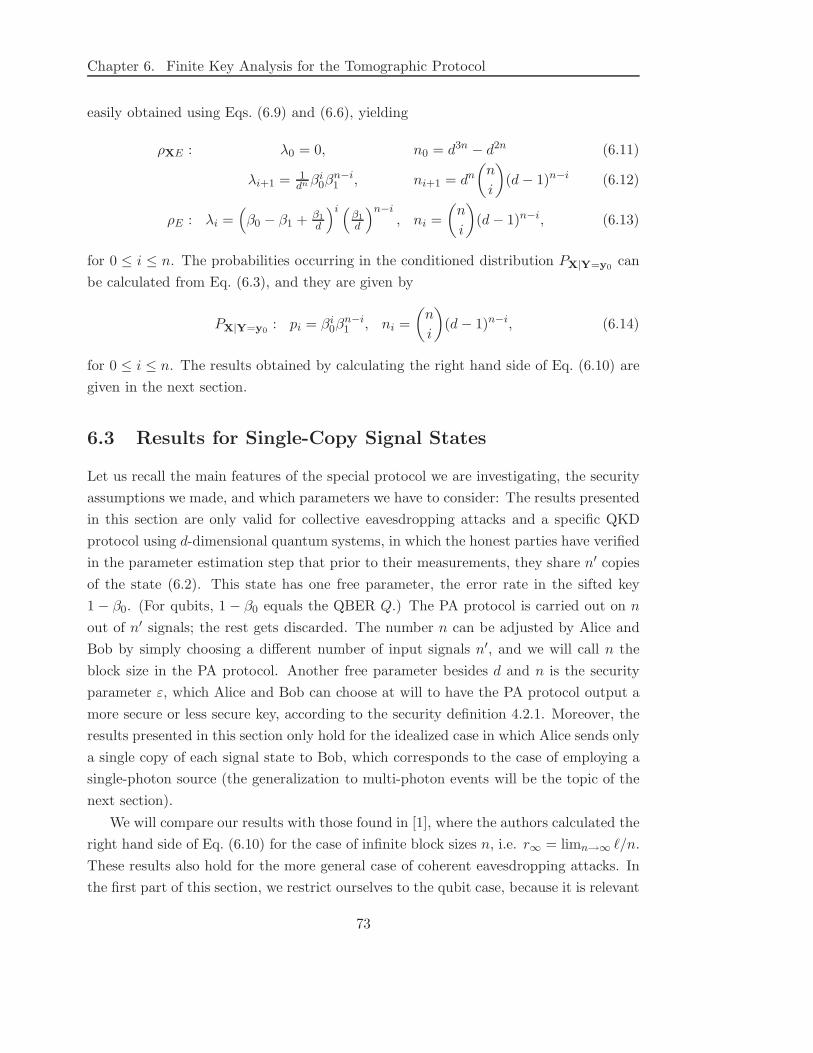
Chapter 6. Finite Key Analysis for the Tomographic Protocol
easily obtained using Eqs. (6.9) and (6.6), yielding
ρXE : λ0 = 0, n0 = d3n − d2n (6.11)
λi+1 = 1dnβi
0βn−i1 , ni+1 = dn
(n
i
)
(d− 1)n−i (6.12)
ρE : λi =(
β0 − β1 + β1
d
)i (β1
d
)n−i, ni =
(n
i
)
(d− 1)n−i, (6.13)
for 0 ≤ i ≤ n. The probabilities occurring in the conditioned distribution PX|Y=y0can
be calculated from Eq. (6.3), and they are given by
PX|Y=y0: pi = βi
0βn−i1 , ni =
(n
i
)
(d− 1)n−i, (6.14)
for 0 ≤ i ≤ n. The results obtained by calculating the right hand side of Eq. (6.10) are
given in the next section.
6.3 Results for Single-Copy Signal States
Let us recall the main features of the special protocol we are investigating, the security
assumptions we made, and which parameters we have to consider: The results presented
in this section are only valid for collective eavesdropping attacks and a specific QKD
protocol using d-dimensional quantum systems, in which the honest parties have verified
in the parameter estimation step that prior to their measurements, they share n′ copies
of the state (6.2). This state has one free parameter, the error rate in the sifted key
1 − β0. (For qubits, 1 − β0 equals the QBER Q.) The PA protocol is carried out on n
out of n′ signals; the rest gets discarded. The number n can be adjusted by Alice and
Bob by simply choosing a different number of input signals n′, and we will call n the
block size in the PA protocol. Another free parameter besides d and n is the security
parameter ε, which Alice and Bob can choose at will to have the PA protocol output a
more secure or less secure key, according to the security definition 4.2.1. Moreover, the
results presented in this section only hold for the idealized case in which Alice sends only
a single copy of each signal state to Bob, which corresponds to the case of employing a
single-photon source (the generalization to multi-photon events will be the topic of the
next section).
We will compare our results with those found in [1], where the authors calculated the
right hand side of Eq. (6.10) for the case of infinite block sizes n, i.e. r∞ = limn→∞ ℓ/n.
These results also hold for the more general case of coherent eavesdropping attacks. In
the first part of this section, we restrict ourselves to the qubit case, because it is relevant
73
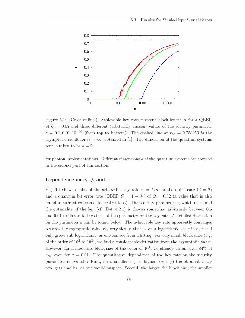
6.3. Results for Single-Copy Signal States
0
0.1
0.2
0.3
0.4
0.5
0.6
0.7
0.8
10 100 1000 10000
r
n
Figure 6.1: (Color online.) Achievable key rate r versus block length n for a QBER
of Q = 0.02 and three different (arbitrarily chosen) values of the security parameter
ε = 0.1, 0.01, 10−10 (from top to bottom). The dashed line at r∞ = 0.758059 is the
asymptotic result for n → ∞, obtained in [1]. The dimension of the quantum systems
sent is taken to be d = 2.
for photon implementations. Different dimensions d of the quantum systems are covered
in the second part of this section.
Dependence on n, Q, and ε
Fig. 6.1 shows a plot of the achievable key rate r := ℓ/n for the qubit case (d = 2)
and a quantum bit error rate (QBER Q = 1 − β0) of Q = 0.02 (a value that is also
found in current experimental realizations). The security parameter ε, which measured
the optimality of the key (cf. Def. 4.2.1) is chosen somewhat arbitrarily between 0.5
and 0.01 to illustrate the effect of this parameter on the key rate. A detailed discussion
on the parameter ε can be found below. The achievable key rate apparently converges
towards the asymptotic value r∞ very slowly, that is, on a logarithmic scale in n, r still
only grows sub-logarithmic, as one can see from a fitting. For very small block sizes (e.g.
of the order of 102 to 103), we find a considerable derivation from the asymptotic value.
However, for a moderate block size of the order of 104, we already obtain over 84% of
r∞, even for ε = 0.01. The quantitative dependence of the key rate on the security
parameter is two-fold: First, for a smaller ε (i.e. higher security) the obtainable key
rate gets smaller, as one would suspect. Second, the larger the block size, the smaller
74
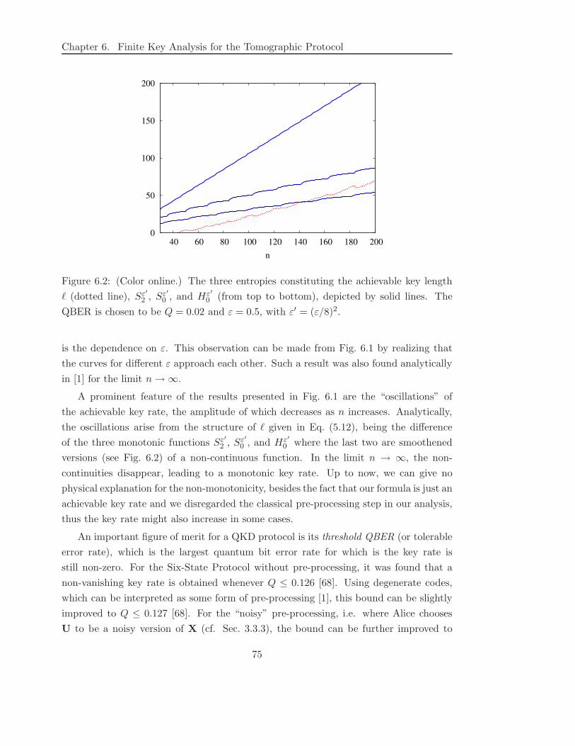
Chapter 6. Finite Key Analysis for the Tomographic Protocol
0
50
100
150
200
40 60 80 100 120 140 160 180 200
n
Figure 6.2: (Color online.) The three entropies constituting the achievable key length
ℓ (dotted line), Sε′2 , Sε′
0 , and Hε′0 (from top to bottom), depicted by solid lines. The
QBER is chosen to be Q = 0.02 and ε = 0.5, with ε′ = (ε/8)2.
is the dependence on ε. This observation can be made from Fig. 6.1 by realizing that
the curves for different ε approach each other. Such a result was also found analytically
in [1] for the limit n→ ∞.
A prominent feature of the results presented in Fig. 6.1 are the “oscillations” of
the achievable key rate, the amplitude of which decreases as n increases. Analytically,
the oscillations arise from the structure of ℓ given in Eq. (5.12), being the difference
of the three monotonic functions Sε′2 , Sε′
0 , and Hε′0 where the last two are smoothened
versions (see Fig. 6.2) of a non-continuous function. In the limit n → ∞, the non-
continuities disappear, leading to a monotonic key rate. Up to now, we can give no
physical explanation for the non-monotonicity, besides the fact that our formula is just an
achievable key rate and we disregarded the classical pre-processing step in our analysis,
thus the key rate might also increase in some cases.
An important figure of merit for a QKD protocol is its threshold QBER (or tolerable
error rate), which is the largest quantum bit error rate for which is the key rate is
still non-zero. For the Six-State Protocol without pre-processing, it was found that a
non-vanishing key rate is obtained whenever Q ≤ 0.126 [68]. Using degenerate codes,
which can be interpreted as some form of pre-processing [1], this bound can be slightly
improved to Q ≤ 0.127 [68]. For the “noisy” pre-processing, i.e. where Alice chooses
U to be a noisy version of X (cf. Sec. 3.3.3), the bound can be further improved to
75
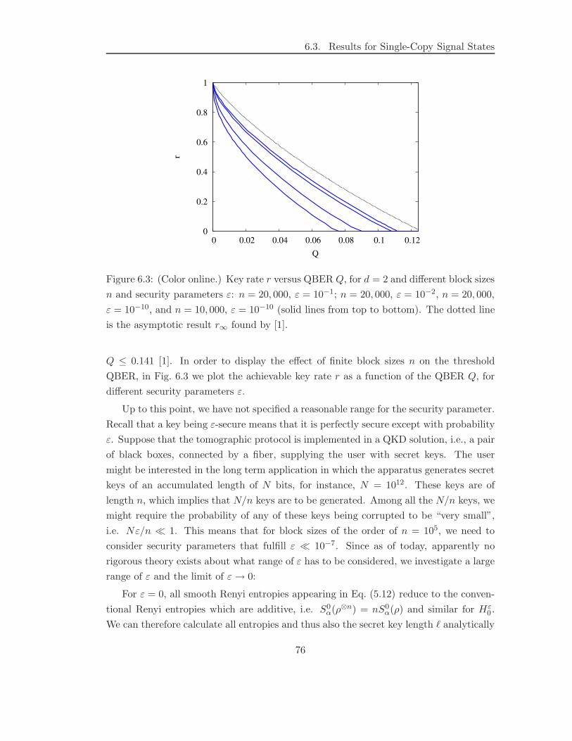
6.3. Results for Single-Copy Signal States
0
0.2
0.4
0.6
0.8
1
0 0.02 0.04 0.06 0.08 0.1 0.12
r
Q
Figure 6.3: (Color online.) Key rate r versus QBER Q, for d = 2 and different block sizes
n and security parameters ε: n = 20, 000, ε = 10−1; n = 20, 000, ε = 10−2, n = 20, 000,
ε = 10−10, and n = 10, 000, ε = 10−10 (solid lines from top to bottom). The dotted line
is the asymptotic result r∞ found by [1].
Q ≤ 0.141 [1]. In order to display the effect of finite block sizes n on the threshold
QBER, in Fig. 6.3 we plot the achievable key rate r as a function of the QBER Q, for
different security parameters ε.
Up to this point, we have not specified a reasonable range for the security parameter.
Recall that a key being ε-secure means that it is perfectly secure except with probability
ε. Suppose that the tomographic protocol is implemented in a QKD solution, i.e., a pair
of black boxes, connected by a fiber, supplying the user with secret keys. The user
might be interested in the long term application in which the apparatus generates secret
keys of an accumulated length of N bits, for instance, N = 1012. These keys are of
length n, which implies that N/n keys are to be generated. Among all the N/n keys, we
might require the probability of any of these keys being corrupted to be “very small”,
i.e. Nε/n ≪ 1. This means that for block sizes of the order of n = 105, we need to
consider security parameters that fulfill ε ≪ 10−7. Since as of today, apparently no
rigorous theory exists about what range of ε has to be considered, we investigate a large
range of ε and the limit of ε→ 0:
For ε = 0, all smooth Renyi entropies appearing in Eq. (5.12) reduce to the conven-
tional Renyi entropies which are additive, i.e. S0α(ρ⊗n) = nS0
α(ρ) and similar for Hε0 .
We can therefore calculate all entropies and thus also the secret key length ℓ analytically
76
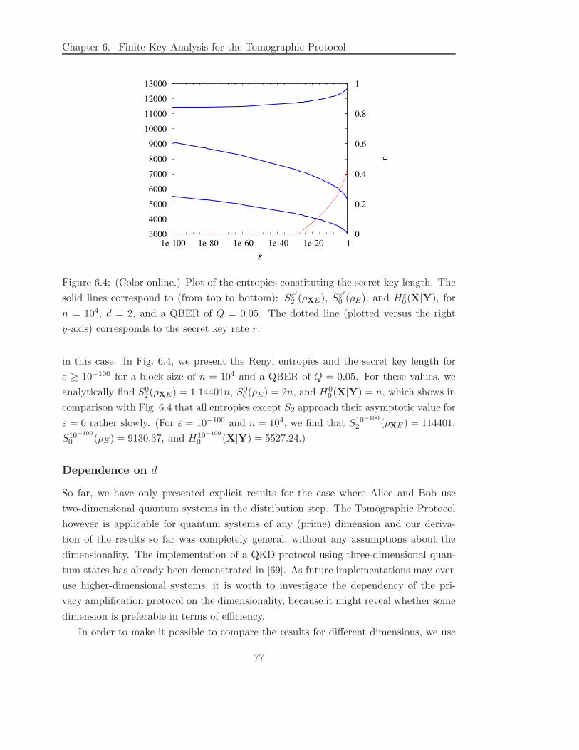
Chapter 6. Finite Key Analysis for the Tomographic Protocol
3000
4000
5000
6000
7000
8000
9000
10000
11000
12000
13000
1e-100 1e-80 1e-60 1e-40 1e-20 1 0
0.2
0.4
0.6
0.8
1
r
ε
Figure 6.4: (Color online.) Plot of the entropies constituting the secret key length. The
solid lines correspond to (from top to bottom): Sε′2 (ρXE), Sε′
0 (ρE), and Hε0(X|Y), for
n = 104, d = 2, and a QBER of Q = 0.05. The dotted line (plotted versus the right
y-axis) corresponds to the secret key rate r.
in this case. In Fig. 6.4, we present the Renyi entropies and the secret key length for
ε ≥ 10−100 for a block size of n = 104 and a QBER of Q = 0.05. For these values, we
analytically find S02(ρXE) = 1.14401n, S0
0(ρE) = 2n, and H00 (X|Y) = n, which shows in
comparison with Fig. 6.4 that all entropies except S2 approach their asymptotic value for
ε = 0 rather slowly. (For ε = 10−100 and n = 104, we find that S10−100
2 (ρXE) = 114401,
S10−100
0 (ρE) = 9130.37, and H10−100
0 (X|Y) = 5527.24.)
Dependence on d
So far, we have only presented explicit results for the case where Alice and Bob use
two-dimensional quantum systems in the distribution step. The Tomographic Protocol
however is applicable for quantum systems of any (prime) dimension and our deriva-
tion of the results so far was completely general, without any assumptions about the
dimensionality. The implementation of a QKD protocol using three-dimensional quan-
tum states has already been demonstrated in [69]. As future implementations may even
use higher-dimensional systems, it is worth to investigate the dependency of the pri-
vacy amplification protocol on the dimensionality, because it might reveal whether some
dimension is preferable in terms of efficiency.
In order to make it possible to compare the results for different dimensions, we use
77
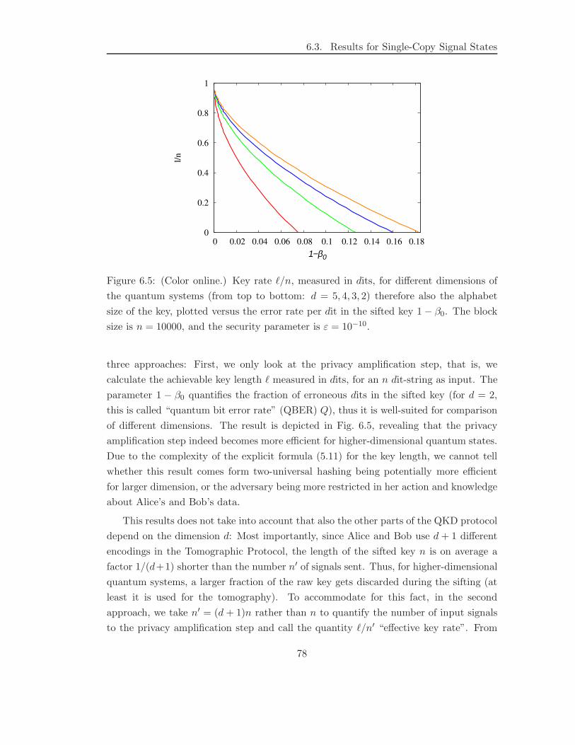
6.3. Results for Single-Copy Signal States
0
0.2
0.4
0.6
0.8
1
0 0.02 0.04 0.06 0.08 0.1 0.12 0.14 0.16 0.18
l/n
1−β0
Figure 6.5: (Color online.) Key rate ℓ/n, measured in dits, for different dimensions of
the quantum systems (from top to bottom: d = 5, 4, 3, 2) therefore also the alphabet
size of the key, plotted versus the error rate per dit in the sifted key 1 − β0. The block
size is n = 10000, and the security parameter is ε = 10−10.
three approaches: First, we only look at the privacy amplification step, that is, we
calculate the achievable key length ℓ measured in dits, for an n dit-string as input. The
parameter 1 − β0 quantifies the fraction of erroneous dits in the sifted key (for d = 2,
this is called “quantum bit error rate” (QBER) Q), thus it is well-suited for comparison
of different dimensions. The result is depicted in Fig. 6.5, revealing that the privacy
amplification step indeed becomes more efficient for higher-dimensional quantum states.
Due to the complexity of the explicit formula (5.11) for the key length, we cannot tell
whether this result comes form two-universal hashing being potentially more efficient
for larger dimension, or the adversary being more restricted in her action and knowledge
about Alice’s and Bob’s data.
This results does not take into account that also the other parts of the QKD protocol
depend on the dimension d: Most importantly, since Alice and Bob use d + 1 different
encodings in the Tomographic Protocol, the length of the sifted key n is on average a
factor 1/(d+1) shorter than the number n′ of signals sent. Thus, for higher-dimensional
quantum systems, a larger fraction of the raw key gets discarded during the sifting (at
least it is used for the tomography). To accommodate for this fact, in the second
approach, we take n′ = (d + 1)n rather than n to quantify the number of input signals
to the privacy amplification step and call the quantity ℓ/n′ “effective key rate”. From
78
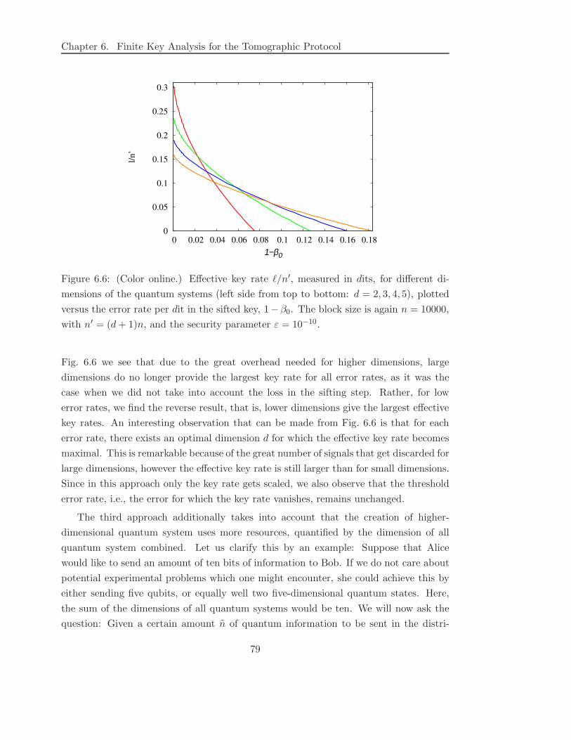
Chapter 6. Finite Key Analysis for the Tomographic Protocol
0
0.05
0.1
0.15
0.2
0.25
0.3
0 0.02 0.04 0.06 0.08 0.1 0.12 0.14 0.16 0.18
l/n
’
1−β0
Figure 6.6: (Color online.) Effective key rate ℓ/n′, measured in dits, for different di-
mensions of the quantum systems (left side from top to bottom: d = 2, 3, 4, 5), plotted
versus the error rate per dit in the sifted key, 1−β0. The block size is again n = 10000,
with n′ = (d+ 1)n, and the security parameter ε = 10−10.
Fig. 6.6 we see that due to the great overhead needed for higher dimensions, large
dimensions do no longer provide the largest key rate for all error rates, as it was the
case when we did not take into account the loss in the sifting step. Rather, for low
error rates, we find the reverse result, that is, lower dimensions give the largest effective
key rates. An interesting observation that can be made from Fig. 6.6 is that for each
error rate, there exists an optimal dimension d for which the effective key rate becomes
maximal. This is remarkable because of the great number of signals that get discarded for
large dimensions, however the effective key rate is still larger than for small dimensions.
Since in this approach only the key rate gets scaled, we also observe that the threshold
error rate, i.e., the error for which the key rate vanishes, remains unchanged.
The third approach additionally takes into account that the creation of higher-
dimensional quantum system uses more resources, quantified by the dimension of all
quantum system combined. Let us clarify this by an example: Suppose that Alice
would like to send an amount of ten bits of information to Bob. If we do not care about
potential experimental problems which one might encounter, she could achieve this by
either sending five qubits, or equally well two five-dimensional quantum states. Here,
the sum of the dimensions of all quantum systems would be ten. We will now ask the
question: Given a certain amount n of quantum information to be sent in the distri-
79
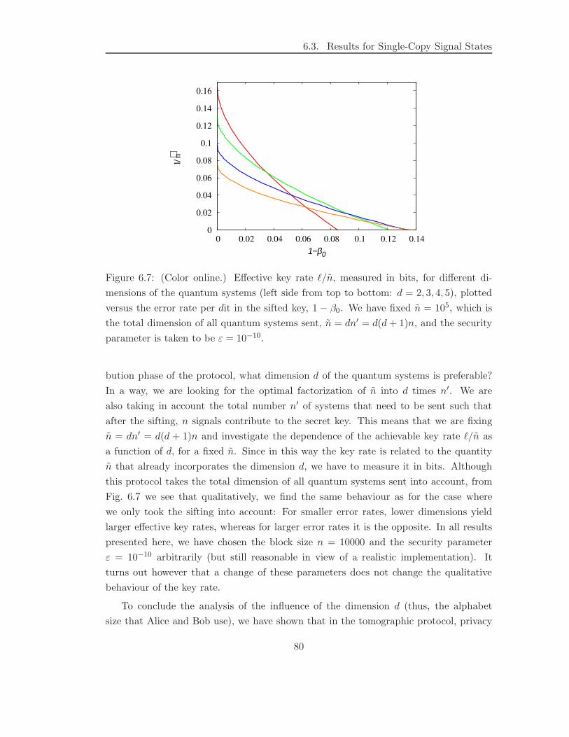
6.3. Results for Single-Copy Signal States
0
0.02
0.04
0.06
0.08
0.1
0.12
0.14
0.16
0 0.02 0.04 0.06 0.08 0.1 0.12 0.14
l/∼ n
1−β0
Figure 6.7: (Color online.) Effective key rate ℓ/n, measured in bits, for different di-
mensions of the quantum systems (left side from top to bottom: d = 2, 3, 4, 5), plotted
versus the error rate per dit in the sifted key, 1 − β0. We have fixed n = 105, which is
the total dimension of all quantum systems sent, n = dn′ = d(d+ 1)n, and the security
parameter is taken to be ε = 10−10.
bution phase of the protocol, what dimension d of the quantum systems is preferable?
In a way, we are looking for the optimal factorization of n into d times n′. We are
also taking in account the total number n′ of systems that need to be sent such that
after the sifting, n signals contribute to the secret key. This means that we are fixing
n = dn′ = d(d + 1)n and investigate the dependence of the achievable key rate ℓ/n as
a function of d, for a fixed n. Since in this way the key rate is related to the quantity
n that already incorporates the dimension d, we have to measure it in bits. Although
this protocol takes the total dimension of all quantum systems sent into account, from
Fig. 6.7 we see that qualitatively, we find the same behaviour as for the case where
we only took the sifting into account: For smaller error rates, lower dimensions yield
larger effective key rates, whereas for larger error rates it is the opposite. In all results
presented here, we have chosen the block size n = 10000 and the security parameter
ε = 10−10 arbitrarily (but still reasonable in view of a realistic implementation). It
turns out however that a change of these parameters does not change the qualitative
behaviour of the key rate.
To conclude the analysis of the influence of the dimension d (thus, the alphabet
size that Alice and Bob use), we have shown that in the tomographic protocol, privacy
80
Chapter 6. Finite Key Analysis for the Tomographic Protocol
amplification is more efficient if greater dimensions are used. We cannot tell whether this
is a consequence of two-universal hashing itself or because of the special restrictions the
eavesdropper encounters due to the tomography. If we take into account that actually
(d + 1)n signals need to be sent in the protocol because of the sifting and define the
key rate with respect to this number, it turns out that for lower error rates, lower
dimensions become favorable, whereas for higher error rates, higher dimensions yield
larger key rates. Moreover, for each error rate there exists a certain dimension which
yields the optimal key rate. Lastly, defining the error rate with respect to the total
dimension d(d+ 1)n of all signals sent (the “resources” needed to establish the key), we
also find that smaller dimensions are favorable for lower error rates and larger dimensions
for larger error rates.
6.4 Inclusion of Multi-Photon Events
In this chapter, we turn towards experimental realizations of QKD protocols and the
security problems that naturally arise in this context. Since most of the experiments
performed so far only employ two-dimensional quantum systems, we restrict our anal-
ysis to the qubit case (d = 2). A common experimental implementation is to use the
polarization degree of freedom of photons as a qubit. Our discussion of the Tomographic
Protocol so far was idealized in the sense that we assumed that Alice sends one of the
signal states |φjx〉 to Bob. This corresponds to the case where Alice prepares exactly
one photon in the corresponding polarization state and sends it to Bob, which is an
unrealistic assumptions because single photon sources do not exist. In reality, Alice uses
an attenuated laser beam with very low intensity such that the average photon number
in each pulse is very low. The light pulse emitted by a laser is a coherent state
|α〉 = e−|α|2/2∞∑
m=0
αm
√m!
|m〉, (6.15)
which is parameterized by some complex number α. Here, |m〉 is a Fock state. If the
phase argα of this coherent state is randomized, we obtain the following state:
ρ =
∫d argα
2π|α〉〈α| =
∞∑
m=0
P (m)|m〉〈m|, (6.16)
which is a mixture of all Fock states wighted with a Poissonian distribution,
P (m) = e−|α|2 |α|2m
m!. (6.17)
81
6.4. Inclusion of Multi-Photon Events
The average photon number of such a pulse is given by m = |α|2. Common QKD
implementations (using these so-called “weak coherent pulses”) employ attenuated lasers
where the average photon number of each pulse is of the order of 0.1. From Eq. (6.17),
we can compute that such pulses are mostly empty, P (0) ≈ 0.905, contain one photon
with probability P (1) ≈ 0.09 and more than one photon with probability∑∞
m=2 P (m) ≈0.005.
Using such a weak coherent pulse-implementation, it follows that Alice does not send
the signal states |φjx〉 to Bob, but rather an unknown number of copies, i.e. |φj
x〉〈φjx|
⊗m
where the number of copies is distributed according to the Poissonian statistic (6.17).
In this situation, the following eavesdropping attack (called “photon number splitting”
(PNS) attack), which cannot be covered by our analysis so far, becomes imminent: Con-
sider that Alice and Bob are connected by a lossy fiber and that Bob’s photo detectors
cannot resolve the photon number (i.e. they can only tell “there was no photon” or
“there were some photons”), which is an assumption that holds in any real-world imple-
mentation. For each pulse sent from Alice to Bob, Eve measures its photon number via
a non-demolition measurement3 [70]. If it is more than one, she splits off one photon,
stores it, and sends the remaining photons to Bob through a lossless fiber. If the pulse
contains no photons, she forwards the vacuum pulse to Bob. If the photon number
is one, she either completely blocks the pulse or performs some single-state attack as
described in Sec. 4.3. She chooses one of these possibilities and the disturbance caused
by the single-state attack in a way that the photon statistics that Bob expects to receive
(he assumes a lossy channel having some yield γ, or attenuation 1 − γ) are maintained.
It is easy to see that such a PNS attack always exists if the yield γ is smaller than the
probability of emitting a multi-photon pulse [40]. In this attack, it is impossible for
Alice and Bob to detect the eavesdropper, because their estimation of the channel yield
is what they expect from a lossy fiber, but Eve has a copy of each signal state of the
multi-photon events. If the QKD protocol employs a simple information reconciliation
step, in which after the distribution, Alice and Bob talk about the encodings used, Eve
can measure all her copies in the corresponding basis and obtains the same classical
data as Alice for signals that were encoded into a multi-photon pulse.
However, under these circumstances, the QKD protocol is not completely insecure.
As long as Alice and Bob can find a proper description of the total system, i.e. the ccq-
state ρXE given by Eq. (6.9), the obtainable secret key length (6.10) can be calculated
also for the weak coherent pulse implementation. The result will certainly be a smaller
key length ℓ than which is obtained for the single-photon case, which tells Alice and
3Using such an operation Eve introduces no errors and thus cannot be detected.
82
Chapter 6. Finite Key Analysis for the Tomographic Protocol
Bob that they need to do “more” privacy amplification, thus sacrificing more raw key.
In the next section, we show how we can find the ccq-state for a weak coherent pulse
implementation of the Tomographic Protocol, under the assumptions of a collective
eavesdropping attack (which is assumed throughout this chapter).
6.4.1 Concept
For the single-photon case, recall that we can express the preparation of the signal
states |φjx〉 in the entanglement-based picture (cf. Sec. 3.2.2), which implies that for
an encoding j chosen by Alice, she prepares
|ψj〉AB =
1∑
x=0
√
PX(x)|x〉A|φjx〉B . (6.18)
It is sufficient to consider some fixed encoding j, because we assume that Alice chooses
them with equal probability and all signals in which Bob chooses a different one are
discarded in the sifting step. In the previous section we have seen that in a weak
coherent pulse implementation, Alice does not prepare the signal states |φjx〉, but rather
a classical mixture of |φjx〉〈φj
x|⊗m
where m is distributed according to a Poissonian
distribution4 P (m). We can incorporate this in Eq. (6.18) by introducing an auxiliary
system R, which is neither controlled by Alice and Bob nor by Eve and which holds the
photon number m, thus purifying the mixture∑∞
m=0 P (m)|φjx〉〈φj
x|⊗m
:
|ψj〉ABR =∞∑
m=0
1∑
x=0
√
P (m)√
PX(x)|x〉A|φjx〉
⊗mB |m〉R. (6.19)
As we have seen in Sec. 4.3, the eavesdropper’s attack is fully described by the attach-
ment of a probe system |0〉E to the signal states underway to Bob and some unitary
operation UBE acting on these two systems, which implies that the state after Eve’s
attack is given by
|ψj〉ABER =
∞∑
m=0
1∑
x=0
√
P (m)√
PX(x)|x〉AUBE |φjx〉
⊗mB |0〉E |m〉R. (6.20)
Since it is possible for Eve to find out the number of photons m in each signal without
introducing any noise, she can actually choose a different unitary operation U(m)BE de-
pending on the photon number. In particular, for m > 1, she can apply a swap operation
4The Poissonian distribution is a special case that occurs for the weak coherent pulse implementation.
Our analysis is valid for arbitrary probability distributions P (m).
83
6.4. Inclusion of Multi-Photon Events
which supplies her with one of the signal states, and some operation U(1)BE for the pulses
containing exactly one photon, as already mentioned in the previous chapter.
Note that this eavesdropping attack is no longer a strictly collective attack, because
we allow the eavesdropper to apply a different unitary operation U(m)BE to each signal
state depending on its photon number. However, this strategy is the most simple gener-
alization of a collective attack to the multi-photon case, since U(m)BE only depends on the
photon number m, and we do not allow Eve to choose an arbitrary unitary operation
for each signal. All signals containing the same photon number will be attacked in the
same way.
Consider the case where Alice employs a source that emits single-photon pulses with
a probability of psingle and multi-photon pulses with a probability of pmulti. During the
sifting, Alice and Bob will discard all empty pulses, which makes it reasonable to define
η = psingle/(psingle + pmulti) to be the rate of single-photon pulses among all non-empty
pulses. Finally, we can define the number of single-photon pulses to be ns = ⌊ηn⌋, and
the number of multi-photon pulses to be nm = ⌊(1 − η)n⌋, where n is total number of
signals after the sifting.5
Let us now investigate the state ρnABE describing all n signals that survive the sifting
step. If we introduce the operators U(m)BE in Eq. (6.20) and project the system R onto a
certain photon number m for each of the n signals, we can separate the total n-signal
state between m = 1 and m > 1:
ρnABE =
[(1∑
x=0
√
PX(x)|x〉AU(1)BE |φj
x〉B |0〉E
)
(h.c.)
]⊗ns
⊗[
∞∑
m=2
P (m)
(1∑
x=0
√
PX(x)|x〉AU(m)BE |φj
x〉⊗mB |0〉E
)
(h.c.)
]⊗nm
(6.21)
=: |Ψsingle〉〈Ψsingle|⊗ns
ABE ⊗ ρmultiABE
⊗nm, (6.22)
where we have defined |Ψsingle〉⊗ns
ABE and ρnm
ABE for the single and multi-photon part,
respectively. Note that Eqs. (6.21) and (6.22) have to be read modulo permutation of
the n subsystems, because the order of the pulses is in general different. Also recall that
we can fix some encoding j, because we are only looking at the signals which survive
the sifting step, and for all those signals Alice and Bob have chosen the same encoding
j.
For the multi-photon part ρ⊗nm
ABE , we have already argued that Eve can split one
signal off |φjx〉〈φj
x|⊗m
B to store it until she learns its encoding j. Then she can measure
5We ignore possible rounding errors and assume that ns + nm = n.
84
Chapter 6. Finite Key Analysis for the Tomographic Protocol
it and obtains the same bit as Bob. Since we assumed that Eve replaces the lossy fiber
between her and Bob by a noiseless one, it is sufficient to forward only one of the photons
in the pulse to Bob, even if there were more than two. Using this strategy, the state
ρnm
ABE is actually also pure and of the form
|Ψmulti〉⊗nm
ABEE′ =
[1∑
x=0
√
PX(x)|x〉AU(1)′
BE |φjx〉B |0〉E|φj
x〉E′
]⊗nm
, (6.23)
where Eve is still free to choose some unitary operation U(1)′
BE on her auxiliary system E
and the remaining photon that she will send on to Bob, and we have introduced a second
system E′ under Eve’s control which stores the copy of the signal state. Comparing
the multi-photon |Ψmulti〉⊗nm
ABEE′ and single-photon part |Ψsingle〉⊗ns
ABE , we observe that
they are essentially identical, the only difference being that for the multi-photon case,
Eve has the additional advantage that she holds the system |φjx〉E′. Moreover, the state
|Ψsingle〉ABE describes exactly the situation discussed in the previous section, which only
dealt with the idealized single-photon case. We therefore make the same assumption as
before, namely that Eve can obtain the purifying system of the state ρAB distributed
between Alice and Bob, now for both the single and multi-photon part. In this way we
can adopt our previous analysis for the state describing all n signals (after the sifting),
|Ψn〉ABE = |Ψsingle〉⊗ns
ABE ⊗ |Ψmulti〉⊗nm
ABE , (6.24)
where we only have to keep in mind that Eve also holds a copy of the signal state for
each of the multi-photon pulses.
For each (non-empty) signal arriving at Alice and Bob, they measure a tomographi-
cally complete POVM, which makes it in principle possible to check for the “effectively”
distributed single signal state
ρeffAB = trE(η|Ψsingle〉〈Ψsingle|ABE + (1 − η)|Ψmulti〉〈Ψmulti|ABE) (6.25)
to be of a certain form. Since otherwise Alice and Bob will abort the protocol, we
assume that Eve prepares the states |Ψsingle〉ABE and |Ψmulti〉ABE such that
ρeffAB = ρdep
AB(β0, β1) := (β0 − β1)|φ+〉〈φ+| + β1
21, (6.26)
that is, the effectively distributed state is a depolarized version of the maximally entan-
gled state |φ+〉 :=∑1
x=0 |xx〉/√
2, in the same way as in the previous section.
The measurements Alice and Bob perform are carried out on the effectively dis-
tributed state (6.25) which is the same as for the idealized single-photon case in the
85
6.4. Inclusion of Multi-Photon Events
previous section. Thus their correlation, described by PXY, given by Eq. (6.3), remains
unchanged. To find the correlation between Eve and Alice’s data X, we need to con-
struct the cq-state corresponding to Eq. (6.9) which we found in the previous section
for the case of single-photon events.
In order to calculate the obtainable key length in a scenario including multi-photon
events, we need to know the structure of the global state (6.24). But Alice and Bob
can only find on which “effective” state (6.25) they performed their measurements. The
global state can thus be any state that is compatible with Eq. (6.25) and Eq. (6.26).
In the next two subsections, we present two different approaches for the determination
of |Ψn〉ABE . In Sec. 6.4.2, we are making the apparent assumption that the single-
photon part trE |Ψsingle〉ABE and the multi-photon part trE |Ψmulti〉ABE are themselves
depolarized states (6.26). Thus also their convex combination via the parameter η in
Eq. (6.25) is a depolarized state. Using this ansatz as a “first guess”, we are able
to calculate the secret key rate for this scenario. However, this approach is not the
most general one, because there are many other states |Ψsingle〉ABE and |Ψmulti〉ABE
which have the desired feature that they lead to the depolarized state in the convex
combination (6.25). One of these possibilities could be favorable for Eve, i.e. it could
lead to a lower obtainable key rate for Alice and Bob. Therefore, in Sec. 6.4.3, we
extend our considerations from Sec. 6.4.2 to a more general case. It will turn out that
it is indeed not sufficient to consider the single- and multi-photon part to be the same
depolarized state — there exists a more general strategy for Eve that leads to a lower
key rate.
6.4.2 Symmetric Splitting
Fixing the form of the effectively distributed state (6.25) to be (6.26) leaves a lot of
freedom in the structure of the states |Ψsingle〉ABE and |Ψmulti〉ABE ; only their mixture
has to be a depolarized maximally entangled state.
In this section, we restrict our attention to the case where both these states are
purifications of the “same” depolarized state, i.e.,
trE |Ψsingle〉〈Ψsingle|ABE = ρdepAB(βs
0, βs1), (6.27)
trE |Ψmulti〉〈Ψmulti|ABE = ρdepAB(βm
0 , βm1 ), (6.28)
only for different parameters βs0,1 and βm
0,1. This assumption is an obvious choice which
fulfills Eq. (6.25), which implies the parameters β0 and β1 measured by Alice and Bob
86
Chapter 6. Finite Key Analysis for the Tomographic Protocol
in the parameter estimation step are given by
β0 = ηβs0 + (1 − η)βm
0 , (6.29)
β1 = ηβs1 + (1 − η)βm
1 . (6.30)
Recall that the parameters β0 and β1 are not independent, rather, they are related by
β0 + β1 = 1.
By Eqs. (6.27) and (6.28), the total state for both the single and the multi-photon
part is the same as for the analysis of the idealized single-photon case in Sec. 6.2. For
this case, we have already derived the cq-state describing Eve’s correlation with Alice’s
data X, and it is given by (cf. also Eq. (6.9))
ρXE =
[∑
x,y
PXY (x, y)|x〉〈x| ⊗ ρxyE
]⊗ns
, (6.31)
with PXY (x, y) = β1 + δxy(β0 − β1) and where
ρxyE = AB〈xy|Ψsingle〉ABE . (6.32)
If we assume that Alice and Bob employ a simple sifting strategy in which they
announce the encoding used for each pulse, Eve will know all key bits that are generated
from the multi-photon part, because she then can measure the stored signals in the
correct basis. This means that the cq-state for the multi-photon part is of the simple
form [1/2∑1
x=0 |x〉〈x| ⊗ |x〉〈x|E ]⊗nm . It follows that for all n signals, the cq-state is
given by
σXE = ρXE ⊗[
1
2
1∑
x=0
|x〉〈x| ⊗ |x〉〈x|E
]⊗nm
, (6.33)
again modulo permutation of the n subsystems (cf. discussion in Sec. 6.4.1).
What is now the maximally obtainable secret key length that can be extracted from
X and Y in the realistic scenario described by Eq. (6.33)? One might expect that the
only contribution to the secret key comes from the single-photon part,
ℓ(σXE)?= ℓ(ρXE). (6.34)
In order to answer this question, we need to evaluate ℓ(σXE), i.e. Eq. (6.10). Note that
σXE = ρXE ⊗ (1r/r ⊕ diag(0, . . . , 0︸ ︷︷ ︸
s
))m, with r = 2, s = 22 − 2, and m = nm. We have
calculated the Renyi entropies appearing in Eq. (6.10) for density matrices of this form
in Sec. 5.3.4, and we already noticed that the correlations between X and Y remain
87
6.4. Inclusion of Multi-Photon Events
unchanged when we are taking multi-photon events into account. Thus we immediately
obtain
ℓ(σXE) ≈ ℓ(ρXE), (6.35)
where the approximation is up to an additive constant of the order of 2−nm . This re-
sult tells us that all nm multi-photon signals do not contribute to the key length at
all, only the single-photon part is important. Due to Eq. (6.27), this part is described
by |Ψsingle〉ABE , the purification of ρdepAB(βs
0, βs1), which is the depolarized state given by
Eq. (6.26). The amount of secret key that can be extracted from this state depends on
the parameter βs0 (or βs
1 = 1 − βs0). But Alice and Bob cannot measure this parameter
directly, only the convex combination β0 given by Eq. (6.29). They can therefore only
infer a lower bound on the secret key length by making the most pessimistic assump-
tion on βs0 compatible with their measurement, which is βm
0 = 1, meaning that most
of the correlations they measured come from the multi-photon part (which does not
contribute). This leads to the lowest possible value for βs0:
βs,min0 =
1
η(β0 − (1 − η)) , (6.36)
or, in terms of quantum bit error rates,
Qmin =1
ηQ, (6.37)
where Q = 1− β0 is the QBER Alice and Bob obtain in the parameter estimation step.
From these considerations we also see that if β0 ≤ 1−η ⇔ Q = 1−β0 ≥ η, all correlations
can be contributed to the multi-photon part, i.e. βs0 = 0 and ℓ = 0. This is a well-known
result [40, 41, 71], meaning that if the error rate in the sifted key is larger than the
probability of creating a single-photon pulse, no secret key can be generated. Another
simple upper bound on the tolerable QBER is obtained by the following consideration:
Remember that the secret key is drawn entirely from the single-photon part (6.27),
which we assumed to be the depolarized state (6.26). If this state is separable, no secret
key can be distilled from it [22, 23]. The condition on the parameters for which this
happens is β0 ≤ 2/3, i.e. Q ≥ 1/3.
As a recap, if Alice and Bob run the Tomographic Protocol in a weak coherent pulse
implementation with a fraction η of single-photon pulses among all n pulses after the
sifting and QBER Q, they can expect to generate a secret key of the same length as if
they ran the protocol using a single photon implementation with only ns = ηn signals
and a larger QBER of Q/η. This result is visualized in Fig. 6.8. Note that if Alice
and Bob would employ decoy pulses [40, 41], they might be able to learn more about
88
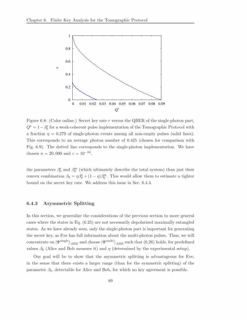
Chapter 6. Finite Key Analysis for the Tomographic Protocol
0
0.2
0.4
0.6
0.8
1
0 0.01 0.02 0.03 0.04 0.05 0.06 0.07 0.08 0.09
r
Qs
Figure 6.8: (Color online.) Secret key rate r versus the QBER of the single-photon part,
Qs = 1−βs0 for a weak-coherent pulse implementation of the Tomographic Protocol with
a fraction η = 0.279 of single-photon events among all non-empty pulses (solid lines).
This corresponds to an average photon number of 0.425 (chosen for comparison with
Fig. 6.9). The dotted line corresponds to the single-photon implementation. We have
chosen n = 20, 000 and ε = 10−10.
the parameters βs0 and βm
0 (which ultimately describe the total system) than just their
convex combination β0 = ηβs0 + (1− η)βm
0 . This would allow them to estimate a tighter
bound on the secret key rate. We address this issue in Sec. 6.4.4.
6.4.3 Asymmetric Splitting
In this section, we generalize the considerations of the previous section to more general
cases where the states in Eq. (6.25) are not necessarily depolarized maximally entangled
states. As we have already seen, only the single-photon part is important for generating
the secret key, as Eve has full information about the multi-photon pulses. Thus, we will
concentrate on |Ψsingle〉ABE and choose |Ψmulti〉ABE such that (6.26) holds, for predefined
values β0 (Alice and Bob measure it) and η (determined by the experimental setup).
Our goal will be to show that the asymmetric splitting is advantageous for Eve,
in the sense that there exists a larger range (than for the symmetric splitting) of the
parameter β0, detectable for Alice and Bob, for which no key agreement is possible.
89
6.4. Inclusion of Multi-Photon Events
We consider the following general6 ansatz for |Ψsingle〉ABE :
|Ψsingle〉ABE =√α1|φ+〉|1〉 +
√α2|φ−〉|2〉 +
√α3|ψ+〉|3〉 +
√α4|ψ−〉|4〉, (6.38)
with∑4
i=1 αi = 1. The marginal state shared by Alice and Bob is thus ρsingleAB =
α1|φ+〉〈φ+|+ · · ·+α4|ψ−〉〈ψ−|, which is separable (i.e., no secret key can be extracted)
if and only if αi ≤ 1/2 for all i.7 Condition (6.25), evaluated for the marginal states
implies that
ρmultiAB =
1
1 − η(ρdep
AB(β0, β1) − ηρsingleAB ), (6.39)
where we again have assumed that the effectively shared state is the depolarized state
(6.26). Inserting the explicit form of ρsingleAB and ρdep
AB(β0, β1) into (6.39) yields
ρmultiAB =
1
1 − η
[(3β0 − 1
2− ηα1
)
|φ+〉〈φ+| +(
1 − β0
2− ηα2
)
|φ−〉〈φ−| (6.40)
+
(1 − β0
2− ηα3
)
|ψ+〉〈ψ+| +(
1 − β0
2− ηα4
)
|ψ−〉〈ψ−|]
. (6.41)
The only assumption we make on ρmultiAB is its positivity, which yields the following
bounds on the parameters αi:
α1 ≤ 3β0 − 1
2η(6.42)
αi ≤ 1 − β0
2ηfor i = 2, 3, 4 (6.43)
A simple bound for the threshold QBER is given by the value of Q for which ρsingleAB
becomes separable. (However, separability is only a sufficient conditions, i.e., there
exist entangled states which also lead to a vanishing key rate.) Thus we look for the
range of β0 which allows αi ≤ 1/2 for all i. The only αi that could possibly be larger than
1/2 is α1, since αi < 1/6 for i = 2, 3, 4 is equivalent to α1 = 1−α2−α3−α4 > 1/2. From
Eq. (6.43), we see that this happens if (1−β0)/(2η) > 1/6, i.e. 1−β0 > η/3. In terms of
the QBER Q, this reads Q ≥ η/3, which needs to be contrasted to the bound Q ≥ 1/3
for the symmetric splitting found in the previous section. This means that for the more
general splitting of the effectively distributed state (6.25) considered in this section, we
can derive a lower tolerable QBER than for the symmetric splitting. This tells us that
the symmetric splitting assumption is not well-suited for a security analysis, because
there exists a strategy for Eve (the asymmetric splitting) which provides Alice and Bob
6This is the most general ansatz because we have shown in Sec. 5.3.2 that the Renyi entropies S2α(ρ)
only depend on the eigenvalues of ρ.7This can be easily verified by consulting the PPT criterion [72].
90
Chapter 6. Finite Key Analysis for the Tomographic Protocol
with a possibly lower key rate for the same QBER. Thus we need to consider the case
where the eavesdropper chooses this attack, which is favorable from her perspective.
To conclude, we have found that for an asymmetric splitting and a measured QBER
of Q ≥ η/3, there exists a separable state ρsingleAB that produces the depolarized state
in the effective mixture (6.25), i.e., no secret key agreement is possible. For the sym-
metric splitting, the corresponding bound reads Q ≥ 1/3, which is too optimistic. This
indicates that the symmetric splitting approach is potentially yields a too optimistic
key rate, since we have shown that it at least yields a too optimistic threshold QBER.
Unfortunately, we cannot calculate the they rate for the asymmetric splitting approach,
as the corresponding density matrices contain too many different eigenvalues, resulting
in an increasing running time of our algorithms. Therefore, we have to leave this issue
unsolved.
6.4.4 Decoy States
The problem that Alice and Bob face whenever they have to deal with multi-photon
pulses is that Eve’s options are greatly increased. We have seen this in the previous
section where the eavesdropper was able to devise a strategy that depends on the photon
number of each pulse. Unfortunately for Alice and Bob, using the standard protocol,
they cannot get enough information about this new strategy to tightly bound the newly
arising parameters, and thus they have to make the most pessimistic assumptions (cf.
Eq. 6.36).
The decoy state protocol aims at solving this problem: By employing a second
photon source with a different photon number statistic, Alice and Bob can measure
more characteristics of their data and can potentially infer the value of all parameters
in the protocol.
Suppose that Alice holds two photon sources which we label a and b. Originally [40,
41], the idea was that pulses from one source (the “signal” source) are used in a stan-
dard (i.e., BB84 or 6-state) protocol to generate the secret key. “Decoy” pulses are
interspersed in between them to probe the eavesdropping strategy. It turned out that
both sources can play an equal role in the key generation, making the naming mislead-
ing. The two sources need to have exactly the same characteristic such as frequency
distribution and polarization, but it is crucial that they have a different photon num-
ber distribution. For simplicity, we assume that they are both Poissonian, but with a
different mean photon number. We denote by ηa,b the fraction of single photon pulses
among all non-empty pulses emitted by source a and b, respectively, and 1 − ηa,b is the
fraction of multi-photon pulses.
91
6.4. Inclusion of Multi-Photon Events
We consider the case where Alice decides for each pulse whether to choose source a
or b, and that Eve cannot distinguish these pulses. However, she can choose her attack
according to the photon number of the pulse. The distributed state is therefore of the
form
ρnAB = ρdep
AB(βs0, β
s1)
⊗nas ⊗ ρdep
AB(βm0 , β
m1 )⊗na
m ⊗ ρdepAB(βs
0, βs1)
⊗nbs ⊗ ρdep
AB(βm0 , β
m1 )⊗nb
m , (6.44)
where na,bs = ηa,bna,b are the number of single photon pulses originating from source a
and b, respectively, and na,bm = (1 − ηa,b)na,b are the corresponding number of multi-
photon pulses. The total number of pulses in source a and b are denoted by na,b, with
na + nb = n. As Alice and Bob can (only) differentiate between pulses from the two
different sources, they measure two effectively distributed states:
ρaAB =
nas
naρdep
AB(βs0, β
s1) +
nam
naρdep
AB(βm0 , β
m1 ) = ρdep
AB(βa0 , β
a1 ), (6.45)
ρbAB =
nbs
naρdep
AB(βs0, β
s1) +
nbm
nbρdep
AB(βm0 , β
m1 ) = ρdep
AB(βb0, β
b1), (6.46)
with
βa,b0 =
na,bs
na,bβs
0 +na,b
m
na,bβm
0 = ηa,bβs0 + (1 − ηa,b)βm
0 , (6.47)
βa,b1 =
na,bs
na,bβs
1 +na,b
m
na,bβm
1 = ηa,bβs1 + (1 − ηa,b)βm
1 . (6.48)
Here, βa,b0,1 are the measurable quantities for Alice and Bob, and the ηa,b are known
because Alice knows the characteristics of her sources. The quantity βs0, i.e., the cor-
relations present in the single-photon pulses, determine the extractable key length, and
need to be determined by Alice and Bob. Since Eqs. (6.47) and (6.48) form a linear
system of equations, Alice and Bob can compute βs0 from their data. This is in contrast
to the scenario depicted in the previous section, where Alice and Bob were not able to
determine the value of these variables exactly, but needed a pessimistic assumption.
As we have shown in Sec. 6.4.2, only the single-photon pulses contribute to the
secret key rate. Thus, by introducing the appropriate cq-states for the different terms
in Eq. (6.44), which are given by Eq. (6.33), we find again that only the single-photon
part, i.e. only ns signals, contribute to the secret key rate. The important parameter
determining the extractable key length is the correlation βs0 in the single-photon part,
which is given by
βs0 =
1
ηa,b(βa,b
0 − (1 − ηa,b)βm0 ) (6.49)
=(1 − ηa)βb
0 − (1 − ηb)βa0
ηa − ηb, (6.50)
92
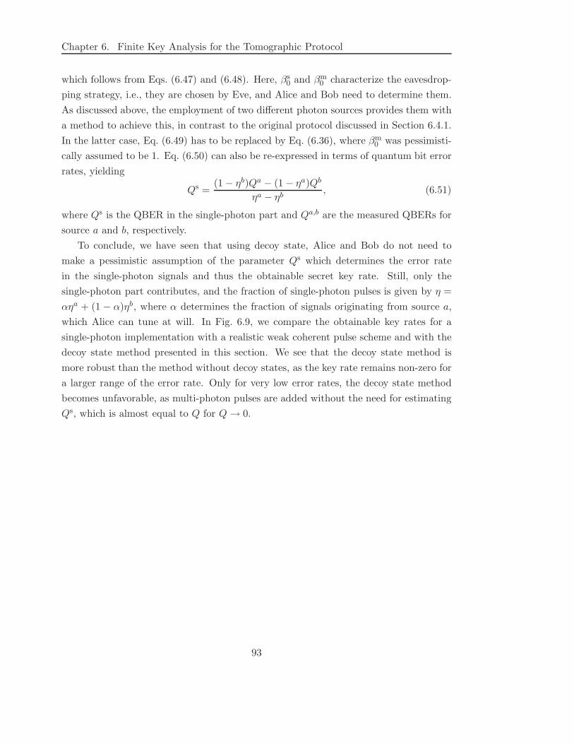
Chapter 6. Finite Key Analysis for the Tomographic Protocol
which follows from Eqs. (6.47) and (6.48). Here, βs0 and βm
0 characterize the eavesdrop-
ping strategy, i.e., they are chosen by Eve, and Alice and Bob need to determine them.
As discussed above, the employment of two different photon sources provides them with
a method to achieve this, in contrast to the original protocol discussed in Section 6.4.1.
In the latter case, Eq. (6.49) has to be replaced by Eq. (6.36), where βm0 was pessimisti-
cally assumed to be 1. Eq. (6.50) can also be re-expressed in terms of quantum bit error
rates, yielding
Qs =(1 − ηb)Qa − (1 − ηa)Qb
ηa − ηb, (6.51)
where Qs is the QBER in the single-photon part and Qa,b are the measured QBERs for
source a and b, respectively.
To conclude, we have seen that using decoy state, Alice and Bob do not need to
make a pessimistic assumption of the parameter Qs which determines the error rate
in the single-photon signals and thus the obtainable secret key rate. Still, only the
single-photon part contributes, and the fraction of single-photon pulses is given by η =
αηa + (1 − α)ηb, where α determines the fraction of signals originating from source a,
which Alice can tune at will. In Fig. 6.9, we compare the obtainable key rates for a
single-photon implementation with a realistic weak coherent pulse scheme and with the
decoy state method presented in this section. We see that the decoy state method is
more robust than the method without decoy states, as the key rate remains non-zero for
a larger range of the error rate. Only for very low error rates, the decoy state method
becomes unfavorable, as multi-photon pulses are added without the need for estimating
Qs, which is almost equal to Q for Q→ 0.
93
6.4. Inclusion of Multi-Photon Events
0
0.1
0.2
0.3
0.4
0.5
0.6
0.7
0.8
0.9
1
0 0.01 0.02 0.03 0.04 0.05 0.06 0.07 0.08 0.09
r
Qs
Figure 6.9: (Color online.) Secret key rate r versus the QBER of the single-photon part,
Qs = 1 − βs0 for a single-photon implementation (dashed line), a weak-coherent pulse
implementation with a fraction η = 0.279 of single-photon events (blue), and a decoy
state implementation (red). For the decoy states, we have used the same parameters as
in [73], that is, ηa = 0.279, ηb = 0.166, and a fraction of α = 3/4 of signals from source
a. We have chosen n = 20, 000 and ε = 10−10.
94
Chapter 7
Conclusion
In this thesis, we have developed a novel method to calculate secret key rates for quantum
key distribution protocols. It consists of algorithms that allow for the explicit calculation
of smooth Renyi entropies, which determine the key rate r by virtue of an expression
found by [1] (see Eq. (5.12)). Our notion of secret key rate is defined with respect to
the privacy amplification step, i.e., it is the ratio of the output (the number of secret
key bits ℓ) and the input (the number of raw key bits n, the block size) of the privacy
amplification step. In particular, our results are valid for any finite value of n (however,
for numerical limitations, we are restricted to values of n . 7 · 104).
As an example application of our algorithms, we investigated the Tomographic Pro-
tocol, a variant of the well-known Six-state Protocol. In its analysis, we made two
assumptions: First, Alice and Bob can verify in the parameter estimation step that the
quantum state they share after the distribution is of a certain form ρdepAB (see Eq. 6.2).
The idea behind this assumption is that Alice and Bob would expect to share this
state in the absence of an eavesdropper if they are connected by a depolarizing channel,
which is a reasonable error model for a realistic channel. The maximally entangled state
|φ+〉 Alice distributes evolves into ρdepAB under the action of this channel. “Verification”
means that we assume that Alice and Bob always share this state, because any instance
in which they find a different state will be treated as an indication for an eavesdropping
attack and the protocol will be aborted. Alternatively, we can interpret the Tomo-
graphic Protocol as the standard Six-state Protocol with an additional restriction on
the eavesdropping attack, namely that it is symmetric, i.e. the noise that it introduces
is white noise, in the same way as for the depolarizing channel. The second assumption
is that the eavesdropper only conducts collective attacks, that is, each signal is attacked
in the same way. There are indications that assuming collective attacks is not really a
restriction, because Alice and Bob can enforce such a high symmetry by only adding a
95
small extra step to the protocol [1, 38, 63].
We are able to calculate the secret key rate for the Tomographic Protocol as a
function of various parameters: The block size n, the quantum bit error rate (QBER)
Q (which is the only free parameter describing the quantum states distributed between
Alice and Bob), the dimension of the quantum systems d, and the security parameter ε.
For a realistic implementation, it is important to assume a finite block size n (the number
of signals that are inputed to the privacy amplification step) and a non-vanishing security
parameter (which is the probability that the final key is insecure). We have found that
the key rate heavily depends on both n and ε: It converges to the asymptotic value r∞
for n → ∞ found in [1], reaching approximately 86% of it at n = 7 · 104 for low error
rates (Q = 0.02) and a security parameter of ε = 10−3. We believe that typical privacy
amplification protocols work with block sizes of the order of 105, therefore our results
suggest that the finiteness of n does not lead to a dramatic decrease of the secret key rate
in a realistic setting. Potentially more severe is the influence of the security parameter
on the key rate for a finite block size, as it was shown that r becomes independent of it
only in the limit n → ∞ [1]. Indeed our results show that the key rate decreases with
decreasing ε. Still, for a realistic error rate of Q = 0.05 and a block size of n = 104, we
have found that the key rate remains non-zero even for very small security parameters
up to ε > 10−28. This is an important result that shows that unconditionally secure
keys can also be created in a realistic scenario. Note that up to now, there is no general
understanding of what are reasonable values to choose for ε.
We extended our analysis of the tomographic protocol to include also multi-photon
events. These are signals send from Alice containing more than one copy of a signal
states, enabling the so-called photon number splitting (PNS) attack. Such events in-
evitably occur in any realistic application relying on weak coherent pulses. Making the
most pessimistic assumptions that the eavesdropper has complete knowledge about all
key bits originating form multi-photon pulses, we have shown that the key rate will
decrease only by a factor of η (the fraction of single photon events) with respect to
an idealized single-photon implementation. However, the estimation of the QBER Q
becomes more involved. Our results suggest that the “real” QBER, which is used for
the calculation of the key rate, is at least a factor of 1/η larger than the QBER which
is estimated from Alice’s and Bob’s data.
Our results show that secret key generation by privacy amplification remains feasi-
ble when taking into account realistic assumptions, namely: The privacy amplification
protocol works with finite blocks of classical data, and the quality of the key is measured
by some security parameter which can be set to a desired value.
96
Appendix A
Numerical methods
In this chapter, we present the numerical methods that were employed to derive the
results presented in Ch. 6. The main task in that section was to find the achievable
key rate for a specific QKD protocol, which involved calculating smooth Renyi entropies
of the quantum states describing Alice’s and Eve’s systems (and of the probability
distribution describing Alice’s and Bob’s correlations). In Sec. 5.3.3, we derived a simple
expression for the Renyi entropies Sε2(ρ), S
ε0(ρ), and Hε
0(X|Y ) in terms of the eigenvalues
and probabilities occurring in ρ and PX|Y , respectively. Since the numerical evaluation
of these expressions are very similar for all entropies, we focus on Sε0(ρ) to present the
details. For ρ ∈ B(Cd), recall that
Sε0(ρ) = log(d− k), (A.1)
where
k =
b−∑
i=1
ni−1 +
⌊ε− s−(b−)
λb−
⌋
, (A.2)
b− = maxr : s−(r) ≤ ε (A.3)
s−(r) =
r∑
i=1
ni−1λi−1. (A.4)
Here, λi and ni with 1 ≤ i ≤ m are the eigenvalues and multiplicities of ρ, respectively,
and 0 ≤ r, b− ≤ m + 1. The specific form of the eigenvalues in given in Eq. (6.13).
The main complication lies in the calculation of b−, for which we cannot give a closed
expression, because we cannot solve (A.4) for r. Therefore, we need to devise an al-
gorithm that checks for all r whether s−(r) ≤ ε and returns the largest one of these.
Unfortunately, it is unfeasible to start from r = 0, increasing r by one in each step and
97

test if s−(r) ≤ ε, because this requires (in the worst case scenario) m + 1 operations.
For the QKD protocol we investigated in Ch. 6, the density matrix ρ is an n-fold tensor
product (cf. Eq. (6.9)), i.e. m is usually of the order of 2n (unless it is pure), where n is
the block size of the privacy amplification protocol, which can easily be of the order of
105 (cf. Sec. 6.2). Thus, this simple approach for finding r needs a number of operations
that scales exponentially in n.
A more desirable approach is to employ a more sophisticated search algorithm to find
b−. This is possible because the elements of the search space, the s+(r), are ordered.
In this work, we implemented a binary search algorithm [74] that cuts the interval
containing the solution in half in each step. Such an algorithm has a running time of
log(m+1), if the search space contains m+1 elements, which is in our case of the order
of log 2n = n. In this way, the running time stays polynomial in the block size of the
PA protocol.
The calculations were performed on standard desktop PCs, equipped with Pentium
4 processors running at 3.2 GHz and 1GB memory. The algorithms were written in
C++, using Ginac’s arbitrary precision library, cln [75]. This is necessary because we
are dealing with very small numbers due to the large size of input density matrices:
The smallest eigenvalue is typically of the order of 2−n (cf. Sec. 6.2). Note that all
calculations performed do not contain any approximations and are exact up to possible
rounding errors. For most of the calculations, it is sufficient to use a precision of 20
significant digits; we verified however for all calculations that a variation of the precision
does not lead to change in the result (the key length, which is of the order of n) of more
than 10−5.
A typical calculation of the secret key length for, say, a block size of n = 20, 000 and
security parameter ε = 10−10 lasts about 10 min. Since the runtime of the algorithms is
only linear in n, there is in principle no limitation for block sizes n to be calculated, as
long as one is investing more computer power and memory. With our limited resources,
we were able to calculate key rates for block sizes up to n = 70, 000, which lasts a couple
of hours, but already uses up all memory. Moving to vector processors or clusters, this
limit could certainly be pushed further, but we do not expect any new insights from
calculating secret key rates for block sizes beyond 105.
98
Bibliography
[1] R. Renner, N. Gisin, and B. Kraus, Phys. Rev. A 72, 012332 (2005).
[2] D. Bruß et al., Phys. Rev. Lett. 91, 097901 (2003).
[3] Y. C. Liang et al., Phys. Rev. A 68, 22324 (2003).
[4] D. Bruß, Phys. Rev. Lett. 81, 3018 (1998).
[5] H. Bechmann-Pasquinucci and N. Gisin, Phys. Rev. A 59, 4238 (1999).
[6] http://www.magiqtech.com.
[7] http://www.idquantique.com.
[8] T. Kelly, Cryptologia 22, 244 (1998).
[9] D. Kahn, The Codebreakers: The Comprehensive History of Secret Communication
from Ancient Times to the Internet (B&T, Charlotte, 1996).
[10] R. Rivest, A. Shamir, and L. Adleman, Communications of the ACM 21, 120
(1978).
[11] C. Papadimitriou, Computational Complexity (Addison Wesley, Amsterdam, 1993).
[12] G. Moore, Electronics 38, (1965).
[13] M. Dusek, N. Lutkenhaus, and M. Hendrych, Progress in Optics 49, 381 (2006).
[14] G. S. Vernam, Journal of IEEE 55, 109 (1926).
[15] C. Shannon, Bell System Technical Journal 28, 656 (1949).
[16] P. Gemmell and N. Naor, Advances in Cryptology–CRYPTO ’93 773, 355 (1993).
99
Bibliography
[17] C. H. Bennett and G. Brassard, in Proceedings of the IEEE International Confer-
ence on Computers, Systems, and Signal Processing, Bangalora, India (IEEE, New
York, 1985), pp. 175–179.
[18] W. K. Wootters and W. H. Zurek, Nature 299, 802 (1982).
[19] A. Ekert, Phys. Rev. Lett. 67, 661 (1991).
[20] J. Clauser, M. Horne, A. Shimony, and R. Holt, Phys. Rev. Lett. 23, 880 (1969).
[21] J. S. Bell, Physics 1, 195 (1964).
[22] A. Acın and N. Gisin, Phys. Rev. Lett. 94, 020501 (2005).
[23] A. Acın, L. Masanes, and N. Gisin, Phys. Rev. Lett. 91, 167901 (2003).
[24] M. Curty, M. Lewenstein, and N. Lutkenhaus, Phys. Rev. Lett. 92, 217903 (2004).
[25] C. H. Bennett et al., Phys. Rev. Lett. 76, 722 (1996).
[26] R. Horodecki, P. Horodecki, M. Horodecki, and K. Horodecki, quant-ph/0702225
(2007).
[27] H.-K. Lo and H. F. Chau, Science 283, 2050 (1999).
[28] P. W. Shor and J. Preskill, Phys. Rev. Lett. 85, 441 (2000).
[29] A. R. Calderbank and P. W. Shor, Phys. Rev. A 54, 1098 (1996).
[30] A. M. Steane, Proc. R. Soc. London A 452, 2551 (1996).
[31] U. M. Maurer, IEEE Transactions on Information Theory 39, 733 (1993).
[32] C. H. Bennett, G. Brassard, C. Crepeau, and U. M. Maurer, IEEE Trans. Info.
Theory 41, 1915 (1995).
[33] C. H. Bennett, G. Brassard, and J.-M. Robert, SIAM Journal on Computing 17,
210 (1988).
[34] N. Gisin, G. Ribordy, W. Tittel, and H. Zbinden, Rev. Mod. Phys. 74, 145 (2002).
[35] J. L. Carter and M. N. Wegman, Journal of Computer and System Sciences 18,
143 (1979).
[36] M. N. Wegman and J. L. Carter, Journal of Computer and System Sciences 22,
265 (1981).
100
Bibliography
[37] R. Renner and R. Konig, in Second Theory of Cryptography Conference, TCC 2005,
Vol. 3378 of LNCS, edited by J. Kilian (Springer, New York, 2005), pp. 407–425.
[38] R. Renner, N. Gisin, and B. Kraus, Phys. Rev. Lett. 95, 080501 (2005).
[39] W. K. Wootters and B. D. Fields, Ann. Phys. (N.Y.) 191, 363 (1989).
[40] W.-Y. Hwang, Phys. Rev. Lett. 91, 057901 (2003).
[41] H.-K. Lo, X. Ma, and K. Chen, Phys. Rev. Lett. 94, 230504 (2005).
[42] A. Peres, Quantum Theory: Concepts and Methods (Kluwer Academic Publishers,
Dordrecht, 1995).
[43] K. Kraus, States, Effects and Operations: Fundamental Notions of Quantum The-
ory (Springer, New York, 1983).
[44] F. W. Stinespring, Proc. Amer. Math. Soc. 6, 211 (1955).
[45] C. Bennett, Phys. Rev. Lett. 68, 3121 (1992).
[46] C. W. Helstrøm, Quantum Detection and Estimation Theory (Academic, New York,
1976).
[47] H.-K. Lo, H. F. Chau, and M. Ardehali, J. of Cryptology 18, 133 (2005).
[48] D. Deutsch et al., Phys. Rev. Lett. 77, 2818 (1996).
[49] I. Devetak and A. Winter, Phys. Rev. Lett. 93, 080501 (2004).
[50] N. Gisin, Helv. Phys. Acta 62, 363 (1989).
[51] L. P. Hughston, R. Jozsa, and W. K. Wootters, Phys. Lett. A 183, 14 (1993).
[52] V. Scarani, A. Acın, G. Ribordy, and N. Gisin, Phys. Rev. Lett. 92, 057901 (2004).
[53] R. Renner and S. Wolf, Lecture Notes in Computer Science 3788, 199 (2005).
[54] N. Gisin, R. Renner, and S. Wolf, Algorithmica 34, 389 (2002).
[55] R. Konig, R. Renner, A. Bariska, and U. Maurer, Phys. Rev. Lett. 98, 140502
(2007).
[56] I. Devetak and A. Winter, Phys. Rev. A 68, 042301 (2003).
101
Bibliography
[57] M. Ben-Or et al., in Second Theory of Cryptography Conference, TCC 2005,
Vol. 3378 of LNCS, edited by J. Kilian (Springer, New York, 2005), pp. 386–406.
[58] R. Renner, Ph.D. thesis, ETH Zurich, 2005.
[59] M. Kleinmann, H. Kampermann, T. Meyer, and D. Bruß, Phys. Rev. A 73, 062309
(2006).
[60] W. Dur, J. I. Cirac, and R. Tarrach, Phys. Rev. Lett. 83, 3562 (1999).
[61] R. Renner, (private communication).
[62] T. Meyer, H. Kampermann, M. Kleinmann, and D. Bruss, Phys. Rev. A 74, 042340
(2006).
[63] R. Renner, quant-ph/0703069 (2007).
[64] J. Schwinger, Proceedings of the National Academy of Sciences of the United States
of America 46, 570 (1960).
[65] S. Bandyopadhyay, P. O. Boykin, V. Roychowdhury, and F. Vatan, Algorithmica
34, 512 (2002).
[66] A. Klappenecker and M. Rotteler, in 7th International Conference on Finite Fields
and Applications (Springer, New York, 2004), Vol. 2984, pp. 137–144.
[67] M. A. Nielsen and I. Chuang, Quantum Computation and Quantum Information
(Cambridge University Press, Cambridge, 2000).
[68] H.-K. Lo, QIC 1, 81 (2001).
[69] S. Groeblacher et al., New J. Phys. 8, 75 (2005).
[70] N. Imoto, H. A. Haus, and Y. Yamamoto, Phys. Rev. A 32, 2287 (1985).
[71] D. Gottesman, H.-K. Lo, N. Lutkenhaus, and J. Preskill, Quant. Inf. Comput. 5,
325 (2004).
[72] A. Peres, Phys. Rev. Lett. 77, 1413 (1996).
[73] Z. L. Yuan, A. W. Sharpe, and A. J. Shields, Appl. Phys. Lett. 90, 011118 (2007).
[74] D. E. Knuth, The Art of Computer Programming (Addison-Wesley Longman, Am-
sterdam, 1999).
[75] http://www.ginac.de/CLN/.
102
Acknowledgements
First and foremost, I would like to thank Prof. Dr. Dagmar Bruß for giving me the
opportunity to work in her group, for the great freedom I experienced during my work,
and for the encouragement I received. Furthermore, I am indebted to the other (also
former) group members Dr. Hermann Kampermann, Dr. Razmik Unanyan, Matthias
Kleinman, Zahra Shadman, and Patrick Skwara for the pleasant atmosphere, countless
discussions, and many advices and enlightments.
Special thanks go to Dr. Renato Renner, Dr. Barbara Kraus, and Prof. Dr. Norbert
Lutkenhaus for helpful discussions.
Finally, I would like to thank my parents and my girlfriend Alexandra for their
understanding and support during the work on this thesis.
103