GAKUTO International Series

Mathematical Sciences and Applications, Vol.32(2010)

Current Advances in Nonlinear Analysis and Related Topics, pp.463–482

GAKKOTOSHO

TOKYO JAPAN

FORCHHEIMER LAW IN COMPUTATIONAL

AND EXPERIMENTAL STUDIES OF FLOW

THROUGH POROUS MEDIA AT PORESCALE

AND MESOSCALE

Ma lgorzata Peszynska

Department of Mathematics, Oregon State UniversityCorvallis, OR, 97331, USA

E-mail: mpesz@math.oregonstate.edu

Anna Trykozko

Interdisciplinary Centre for Mathematical and Computational Modelling, University of Warsawul. Pawinskiego 5a, 02-106 Warsaw, Poland

E-mail: a.trykozko@icm.edu.pl

and

Wojciech Sobieski

Faculty of Technical Sciences, University of Warmia and Mazury in Olsztynul. Oczapowskiego 11, 10-957 Olsztyn, Poland

E-mail: wojciech.sobieski@uwm.edu.pl

Abstract. We propose an algorithm for upscaling of flow with inertia within a multiscaleframework ranging from porescale (microscale) to lab scale (mesoscale). In particular, wesolve Navier-Stokes equations over complex pore geometries and average their solutionsto get flow parameters at mesoscale. For periodic geometries, this is exactly the ideaof homogenization. As concerns averaging, we follow the methodology derived in ourprevious work, which was succesful in deriving stable parameters for flow with inertia,i.e., Forchheimer flow model, at mesoscale. The focus of this paper is twofold: i) to verifythat results of our computational experiments are stable in the homogenization limit, andii) to compare those virtual results with those from physical experiments.

AMS Subject Classification 35Q35, 76S05, 68U20c⃝Gakkotosho 2010, GAKKOTOSHO CO.,LTD

464

1 Introduction

In many mathematical models of important phenomena with real-life applications, onefaces the challenge of multiple spatial and temporal scales. This is true in particular inthe study of flow and transport in porous media, which is important in environmentalstudies, geophysics, reservoir engineering, chemical engineering, and medicine.

The multi-scale nature of porous media is well known. In this work we are goingto deal mainly with microscale, also referred to as porescale, and with lab-scale, alsocalled mesoscale or Darcy scale. At microscale, a porous medium is represented as arigid solid skeleton with fluid flowing through pores (void space). At mesoscale, it is seenas a continuum: a permeable material. Other scales relevant to porous media includemacroscale which is appropriate in large regional groundwater flow models and in oilreservoir engineering. Passage from mesoscale to macroscale is known as upscaling and willnot be addressed here. See [37, 45, 25] for general overview and references and specifically[22, 29] for results on upscaling Forchheimer flow from mesoscale to macroscale.

In this work following [35, 34] we are interested in flow at micro- and meso-scale.The flow through porous media at microscale is described, in general, by Navier-Stokesequations, and the flow at mesoscale is described by Darcy’s law or its extensions.

Darcy’s law [6] postulates a linear relationship between pressure drop and flow rate.It has been shown first in [19] that its validity is restricted to a limited range of flowvelocities quantified by a Reynolds number Re. In [19] it is proposed that the inertiaeffects start to play a significant role for higher values of Re and a linear law is not validany more. To account for inertia terms, Forchheimer proposed a quadratic correctionterm. The coefficient β associated with the correction term is, however, hard to findexperimentally and has been the subject of many discussions and controversies; see thediscussion in [40]. In fact, there is actually no agreement even as concerns the form of thenonlinear correction. The mathematical theory of homogenization states however that,as long as a certain scaling with a parameter ϵ denoting the relative grain size to the sizeof the domain is applied, one can relate the local averages of porescale computations tosome flow model at mesoscale.

These difficulties and ambiguities motivated on one hand our experimental work [40]on flow with inertia and on the other hand the idea of a computational (virtual) laboratoryin which we connect the flow at microscale with the averaged flow at mesoscale [35, 34].The latter idea has not been feasible until recently. However, thanks to a significantincrease in computational power in the last decade, numerical solutions of Navier-Stokesequations in pore geometries, i.e. at microscale, can be now obtained not only for onepore, but actually for a domain composed of a considerable number of pores. While ourinitial work [35] was successful in connecting the porescale to mesoscale, it was clear thatthe numerical approximation of the solutions to Navier-Stokes equations required care toensure convergence and stability [34].

The next natural research question is to relate these results to their mathematicalfoundations and to verify i) whether the ideas of homogenization and, in particular, thescaling of coefficients, can be interpreted using the computational models and, in otherwords, whether they remain stable with grain diameters going to 0. In addition, we set outto verify ii) how the coefficients obtained in computational experiments compared with

465

experimental values from our other work on flow with inertia [40]. These two questionsare addressed in this paper.

If answers to i) and ii) are affirmative, our computational method can be seen as aprototype of a virtual laboratory which can be used en lieu of physical experiments. Wedescribe the steps to verify i) and ii) below.

First we set up the virtual laboratory. We start by defining a reference microscalegeometry for the porous medium. We mention several methods which can help to iden-tify porescale geometry including micro-computerized tomography images [8], models ofvirtual reconstruction of porous samples based on modelling of geological processes ofrock formation [28], random structures generation [27], and different variants of regularstructures of solid-void space distribution [12, 21, 4]. However, in this paper we restrictourselves to a periodic geometry appropriate for i). We consider grain diameter of asimilar size to those measured in experiments and use the simplest virtual microstruc-ture consisting of equally distributed spheres/circles. The flow is driven by boundaryconditions; this is not a standard set-up for homogenization.

Second, given the microscale geometry, we simulate fluid flow through the pores nu-merically. We use a continuum level method, i.e., we use a numerical discretization ofNavier-Stokes equations. These are well studied, but their use in complex geometriesrequires fine grids and is, in general, nontrivial. In our approach we use a finite-volumediscretization [43]. Alternative non-continuum methods include Lattice-Boltzman meth-ods [28] and pore network models [33, 13].

Third, we use averaging to get macroscale values of velocity and pressure drop, andcalculate the values of effective coefficient of proportionality called conductivity. Thiscalculation is only superficially straightforward, since the stability of results with respectto grids and algorithms over a large range of Reynolds numbers must be ensured.

The results of these three steps are applied in a series of experiments to periodicgeometries of a decreasing value of ϵ. Based on these we verify i). Next, to answer ii), wecompare the results of the reference case to the experimental data. Details, theoreticalframework and discussion are shown below.

To our knowledge, the approach in this work following [35, 34] is the first such result inthe literature. Related work in [3, 11, 30, 12] addressed the qualitative character of inertiaat porescale without deriving upscaled models, discussing homogenization, or comparisonwith experimental data.

This paper is organized as follows. In Section 2 we recall mathematical models of flowat micro- and mesoscale. Computational laboratory concepts and averaging techniquesare described in Section 3. Section 4 discusses the homogenization aspects of the project,i.e., addresses i). Special attention is paid to the issue of boundary conditions which aredriving the flow instead of external forces. In Section 5 we address ii), i.e., we compareexperimental data with values computed for the synthetic porous medium. We concludeand outline open questions in Section 6.

466

2 Mathematical models at porescale and macroscale

Let Ω ⊂ Rd, d = 2, 3 be an open bounded domain occupied by a porous medium and thefluid within. For simplicity in what follows only d = 2 will be considered. We denote by(q)i, i = 1, 2 the components of a vector q ∈ R2, and e1 and e2 denote unit vectors of acoordinate system.

2.1 Flow at porescale

At porescale the solid and liquid phases are distinct. Let ΩF be the part of Ω occupiedby the fluid and denote the solid by ΩR. Let Γ = ∂ΩF ∩ ∂ΩR be the rock–fluid interface,and denote the external boundary of flow Γext := ∂ΩF ∩ ∂Ω; it is composed of the inflowΓin and outflow Γout parts. Also, we have ∂ΩF = Γext ∪ Γ.

We consider an incompressible Newtonian fluid of velocity u and pressure p, flowingin ΩF . The fluid’s viscosity is denoted by µ and the (constant) density by ρ.

The flow is driven primarily by external boundary conditions, such as in a lab core.We prescribe the inflow velocity at Γin with maximum denoted by uin and parabolic shapebetween the walls. On Γout we impose a numerical outflow condition [43]. On internalboundaries Γ we assume the no-slip condition u = 0.

Reynolds number Re = |u|δµ

, where δ stands for a characteristic length in the domainof the flow, e.g., width of a channel or the diameter of porous grains, is routinely usedto distinguish between different flow regimes [44, 24, 26, 40]. In porous media the linearlaminar flow regime corresponds to Re < 1, the nonlinear regime is for 1 ≤ Re < 10,and turbulence may occur for Re ≥ 10 [39, 6]; the turbulence rarely occurs in porousmedia. The values of Re characterizing the flow regimes given above vary depending ona quantitative definition of the end of each regime, on a structure of a medium, and on adefinition of the Reynolds number itself [44, 40]. In our computational experiments thevalue of Re is related to the inflow velocity uin.

Now we discuss the mathematical model for flow at microscale (porescale). For steady-state flow, in the absence of forces and mass source/sink terms, the momentum and massconservation in Eulerian frame are expressed by the Navier-Stokes system [5]. Aftersetting for simplicity in the presentation ρ ≡ 1 and rescaling variables with µ, we havethe stationary Navier-Stokes equations

∇ · u = 0, x ∈ ΩF , (2.1)

u · ∇u − µ u = −∇p, x ∈ ΩF . (2.2)

An alternative formulation in terms of the vorticity vector ω = ∇ × u and the streamfunction ψ defined by u = ∇× ψ was considered in [35].

For small Re, viscous effects dominate and the nonlinear convective, i.e., inertia termsassociated with u· are dropped from (2.2), resulting in the linear Stokes approximation;see Section 4.

467

2.2 Flow at Darcy scale

At Darcy (lab scale/mesoscale) the boundaries between ΩF and ΩR are not recognized.Instead, the average flow in Ω characterized by average pressure P and velocity (flux)U is considered. Mass conservation ∇ · U = 0,x ∈ Ω. The flow is driven by boundaryconditions which average porescale boundary conditions.

Darcy’s law is a linear momentum equation at mesoscale

K−1U = −∇P, x ∈ Ω, (2.3)

where K is the conductivity tensor; its values are measured experimentally [6]. Moreprecisely, K may be expressed as K = κ

µwith absolute permeability tensor κ reflecting

properties of the medium. In what follows, notions of K and κ will be used alternatively.

In general, K =

[K11 K12

K21 K22

]for flow in d = 2 dimensions, and is symmetric. If co-

ordinate axis are aligned with the principal directions of the porous medium, then K isdiagonal. Furthermore, in isotropic media K is diagonal and K11 = K22. Due to largeviscous dissipation and interstitial effects common in porous media, Darcy’s law is a goodapproximation for a large class of flow phenomena.

For large flow rates Darcy’s law is not accurate. In the nonlinear laminar regime withsignificant inertia a non-Darcy model which extends (2.3) reads

K−1(U)U = −∇P, x ∈ Ω. (2.4)

The Forchheimer model K−1(U) := K−1 + β|U | was first proposed for the scalar caseΩ ⊂ R [19]; it was extended to multidimensional isotropic media [16, 6, 39, 14] and isused in petroleum industry around wells [17] in the form

K−1(U)U :=(K−1 + β|U|

)U = −∇P, x ∈ Ω. (2.5)

The form of nonlinear map K for general anisotropic 2D and 3D media has been thesubject of theoretical research [31, 20, 23, 10]. Experimental studies [26, 40] focus onidentification of flow regimes. There are controversies and inconsistencies concerning theform of K as well as the values of the coefficient β.

3 Computational model

Now we recall the set-up of our virtual lab described originally in [35, 34]. The compu-tational lab is restricted in this paper to d = 2. The case of d = 3 is not substantiallyharder logically but requires much more pre-processing and computational power. Onceall elements of the virtual laboratory are well understood, we will consider 3D geometries.

Our computational laboratory includes two elements: fluid flow simulations at porescaleand upscaling to mesoscale. We discuss both below.

The aim of upscaling is to derive models with effective coefficients at higher scale andto incorporate as many processes and nonhomogeneities from the lower scale as possible.There are two main methodologies for upscaling: homogenization- and volume averaging-based approaches.

468

The homogenization theory provides theorems on convergence of the averages of lower-scale quantities to the higher scale counterparts together with appriopriate formulas[7, 38]. A good control of the error estimates and qualitative analysis is provided. Ho-mogenization is essentially restricted to periodic geometries at lower scales; this may bean important limitation. However, in periodic geometries, the computations may be per-formed on an elementary cell only. The volume averaging based techniques belong toa second group of methods used in upscaling. There are no restrictions with respect togeometry patterns provided the region of averaging, i.e., REV ≡ Representative Elemen-tary Volume, is large enough to ensure stability of averaged quantities, and small enoughnot to be influenced by boundary conditions. Effective parameters are computed basedon volume averages of microscale variables. In Section 4 we discuss the homogenizationapproach and link the volume averaging approach to convergence results provided byhomogenization theory.

Now we go over the sequence of steps performed in the computational laboratory.We start by defining the geometry of a synthetic porous medium at microscale and anappropriate grid at mesoscale. The subscript h is associated with numerical solutions atmicroscale and H applies at mesoscale.

A synthetic porous medium is defined by a regular structure of equally distributedcircles of equal radii representing solid grains; while ΩF is the space between the grains, seeFigure 2. We define an unstructured mesh of triangular elements over ΩF ; the parameterh is the maximum diameter of the mesh elements. We solve the steady-state Navier-Stokes equations (2.1)–(2.2) numerically and obtain uh and ph. The method is based onfinite-volume discretization [18, 43]. Mesh generation and computations are performedunder ANSYS FLUENT software [18].

Figure 1: Macrocells used in upscaling

Next we consider mesoscale grid over Ω. It is often the case that upscaling is per-formed with respect to a specific discretization scheme to be implemented at a higherscale. Our approach [35, 34] is inspired by the conservative cell-centered finite difference(CCFD) method and resembles the ideas of mesoscale upscaling in porous media from[15], providing at the same time a bridge to macroscale as in [22]. In CCFD the cellcenters are associated with pressure unknowns PH and the cell edges are associated withvelocity unknowns UH . We impose a similar structure in our averaging approach.

Assume we are concerned with flow in ΩF around some point X0 ∈ Ω0 ⊂ Ω. In orderto define the averages over Ω0, a mesoscale discretization needs to be superimposed overthe microscale grid, see Figure 1. Solving numerically the Navier-Stokes equations (2.1)–(2.2) we obtain uh, ph. Next we identify the values UH , PH |X0 at Darcy scale with some

469

averages ⟨ujh⟩, ⟨p

jh⟩ over Ω0 ⊂ Ω. The set Ω0 is a proper subset of Ω, we make sure that

the boundaries of Ω0 are far enough from inlet and outlet boundaries Γin,Γout of Ω toavoid any numerical boundary artifacts.

Now, in order to compute K, a discrete form of (2.3) and of ∇PH is needed. In[15] such values are inferred from boundary conditions. In our case this is not directlypossible since the boundary conditions are defined at porescale. Instead, we partition Ω0

into pairs of cells, ΩL, ΩR, and ΩT , ΩB, see Figure 1. The first component of the gradientis calculated as GLR = PL−PR

xR−xL, where PL = ⟨ph⟩ΩL

, PR = ⟨ph⟩ΩR, with xR and xP denoting

x-coordinates of centers of gravity of ΩL and ΩR. Analogically we get GBT = PB−PT

yT−yB. The

velocity is computed as Uj = ⟨ujh⟩Ω0 and it has components (U j

LR, UjBT ).

In order to find four unknown components of K from U = −K∇P , we need twoindependent sets of data for Uj and for the associated pressure drops G so that thesystem

U1LR

U1BT

U2LR

U2BT

=

G1

LR G1BT

G1LR G1

BT

G2LR G2

BT

G2LR G2

BT

K11

K12

K21

K22

(3.6)

has a unique solution.

To generate data U1,U2 and the associated pressures, we set up virtual flow experi-ments j = 1, 2 with boundary conditions forcing the flow in different directions for eachj. The easiest is to ensure that the (global) flow directions are essentially orthogonal.

Note that we do not explicitly impose the symmetry K12 = K21 which is a funda-mental property of the tensor K. Rather, we expect it to hold for computational results.A numerically confirmed symmetry is one of the measures of the quality of numericalexperiments.

Repeating the experiment described above for increasing values of Re, we obtain asequence of corresponding values of K in (2.4) and are able to compute β by inversemodeling.

4 Homogenization approach

Now we discuss our computational experiments within the homogenization framework inorder to address issue i) from the Introduction. We use notation from Section 2 and thetraditional notation for Sobolev spaces Hk(Ω) [1, 42].

First we discuss Stokes flow which is a linearization of (2.1), (2.2). The flow is drivenby external forces appearing in the momentum equation (4.7), and by external boundaryconditions (4.9). The mathematical model for Stokes flow is given by

∇p− µ u = f , x ∈ ΩF , (4.7)

∇ · u = 0, x ∈ ΩF , (4.8)

u = g, x ∈ ∂ΩF , (4.9)

470

where f ∈ (H−1(ΩF ))d and g ∈ (H1/2(∂ΩF ))d are given. We require for well-posednessthat the boundary ∂ΩF is C2 smooth [42]1, and that the compatibility condition∫

∂ΩF

g · n = 0 (4.10)

is satisfied.

Remark 4.1 Based on these conditions it is shown in [42], [Chapter 1, Theorem 2.4],that there exists a unique solution (u, p) ∈ (H1(ΩF )d, L2(Ω)/R) to (4.7), (4.8), (4.9). Iff,g vanish simultaneously, it follows that p ≡ const,u ≡ 0.

a) b) c) d)

Figure 2: Homogenization approach a) elementary cell, b) Ωϵ1F , c) Ωϵ2

F , and d) Ωϵ3F

We now give consideration to the terms f,g driving the flow.In the problem of interest to us which is determination of the flow coefficients at

lab scale, we envision a computational experiment simulating a physical experiment in alaboratory in which a core is filled by a porous medium and a fluid. The fluid flows dueto a pressure difference which can be measured. After the flow rates are measured, theconductivity coefficient is determined as a proportionality constant between the flow rateand pressure drop. It is not necessary in such experiments to consider gravity since thecore can be placed horizontally; in this case f ≡ 0, g ≡ 0.

As concerns g, it needs to be prescribed on ∂ΩF = Γext ∪ Γ = Γin ∪ Γout ∪ Γ, and weshall prescribe g that is continuous on Γin ∪ Γ which then satisfies g ∈ (H1/2(∂ΩF ))d. Itis customary to prescribe the no-slip condition g|Γ = 0 on the walls of porous medium∂ΩR, and from this follows that the condition on Γext must honor the compatibility thatg|Γext∩Γ = 0. It remains to define g|Γext .

For the inflow condition g|Γin, we impose the “usual” parabolic profile between the

walls whereby g vanishes in contact with the walls ∂ΩR, and achieves maximum in themiddle of a pore throat; on straight inflow edges its tangential component is zero. Asconcerns g|Γout , it is important to recall that in numerical experiments one customarilyprescribes inflow velocity at Γin and a numerical outflow condition on Γout [43], Section6.2]. This technique avoids numerical instabilities and formation of artificial boundarylayers. In other words, we do not prescribe g|Γout in numerical experiments.

However, in the discussion below we shall assume that that g as a trace of u is smoothenough on the entire ∂ΩF . While it is possible to formulate another well-posedness resultfor the actual problems solved numerically, we will not attempt it.

1It is actually shown in [42] that the boundary only has to be Lipschitz.

471

4.1 Homogenization for homogeneous boundary conditions

Now consider the situation in which ΩϵF has periodic geometry with period size ϵ, see

Figure 2. It was observed in [38] that the solutions to (4.7)-(4.8)-(4.9) should be periodic,or at least that they should have some periodic components. Additionally, it was postu-lated that the pressure is close to its local averages and that velocities can be averaged togive an idea of prevailing flow conditions. This “closeness” should become “better” if ϵ issmaller. The technique of homogenization then attempts to derive the effective equationssatisfied by those averages. It turns out that these equations are Darcy’s law (2.3).

In other words, we approximate the solution to a Stokes problem on ΩϵF by a solution

to Darcy problem at lab scale posed in Ω. To deal with the fact that fluid/rock boundariesare not recognized at lab scale, one extends the velocities from Ωϵ

F to ΩϵR by zero (they

already satisfy a no-slip condition on Γ); the pressures are extended by their averages; see[2]. One also computes the conductivity coefficient by averaging some auxiliary solutionsdependent on pore geometry.

The formal asymptotic expansions and calculations demonstrating that Darcy’s lawis effectively an average of Stokes momentum equation, were first shown in [38] and werecomplemented by a proof of convergence in [41]. The convergence was L2-weak for ve-locities and L2-strong for pressures. A stronger result using a corrector was proved byAllaire; see details and references in [[2], Prop.1.2]. The above calculations and conver-gence proofs are applicable to flow problems driven by an external force field f ≡ 0 andrequire homogeneous boundary conditions on Γext.

In this paper we are interested in discussing f ≡ 0, and nonhomogeneous boundaryconditions on Γext. In what follows we revisit the ideas of homogenization in this context,first considering the case in which f ≡ 0,g ≡ 0.

4.2 Asymptotics for homogeneous boundary conditions

We briefly recall the ansatz for formal asymptotic expansions in which each variable isexpanded in powers of ϵ. The usual asymptotic technique is to discern between globaland local spatial coordinates x and y = x

ϵ, with x ∈ Ω, y ∈ Y , where Y is a unit periodic

cell, and to pose equations in which differential operators have components with respectto x and y appropriately scaled, e.g., ∇ 7→ ∇x + 1

ϵ∇y. Additionally, all components of

variables are assumed Y periodic with respect to y ∈ Y :

pϵ(x) = p0(x) + ϵp1(x, y) + . . . , (4.11)

uϵ(x) = u0(x, y) + ϵu1(x, y) + . . . . (4.12)

Next, the idea is to substitute (4.11), (4.12) into (4.7), (4.8) and to match the termsappearing at the same orders of ϵ. It is very important [38, 23, 9] to impose the scalingµ = ϵ2µ0 on viscosity, where µ0 is some reference value. For simplicity, we set µ0 ≡ 1 asin [38].

The calculations lead to an equation satisfied by u0, p0

∇xp0 + ∇yp1 + yyu0 = f , (4.13)

∇y · u0 = 0. (4.14)

472

If the homogeneous boundary conditions are imposed, then one obtains after averaging(4.14) that ∇x · ⟨u0⟩ = 0 which is the statement of mass conservation. However, merelyaveraging (4.13) does not yield momentum equation for u0. Instead, consider multiplyingit by a Y -periodic test function ψ ∈ H1,∇ · ψ = 0, ψ|Γ = 0, and integrating over Y . Inthis variational formulation of (4.13) one discovers that for any such ψ,∫

Y ∩ΩF

(−f + ∇xp0 + yyu0) · ψ = 0, (4.15)

where we have eliminated the second term by integrating by parts and periodicity.To decouple further, the ansatz u0 =

∑i(fi − ∂po

∂xi)ωi conveniently separates scales in

(4.13) and (4.15) to yield a local problem to be solved for Y -periodic ωi, which can bewritten in the strong form as

∇yπ + yyωi = ei, (4.16)

∇ · ωi = 0. (4.17)

The global mode of variation of u0, or rather its average ⟨u0⟩Y over Y , satisfies

⟨u0⟩Y = K(f −∇xp0). (4.18)

Now, to find K, one should first solve the generic problems (4.16)-(4.17) over Y fori = 1, 2, i.e., in at least 2 experiments when d = 2, and find K from its definition

(K)ij = (⟨ωi⟩Y )j. (4.19)

Alternatively, if (f −∇xp0) is known, we could calculate K from matching both sidesof (4.18). It is clear however that we need two experiments to get K. We extend thisobservation now.

We propose to solve the flow problem (4.7)–(4.9) for u, p over a contiguous union Ym

of m translations of periodic cells Y denoted each by Yj so that Ym = Y1 ∪ Y2 . . . ∪ Ym ⊂Ωϵ

F . Assuming ϵ is small enough and m not too large with respect to diam(Ω), we canapproximate ⟨p⟩m×Y ≈ ⟨p0⟩Ym , ⟨u⟩Ym ≈ ⟨u0⟩Ym . Next, since p0 varies with x, i.e. with jindexing Yj, we do not have ⟨p0⟩Ym ≈ ⟨p0⟩Yj

. However, if f does not vary too much withx i.e. within Ym, then ⟨u0⟩Ym ≈ ⟨u0⟩Yj

and ⟨f −∇xp0⟩Ym ≈ ⟨f −∇xp0⟩Yjfor any j.

Now the following calculation makes sense. Add (4.18) over all members of Ym toobtain

⟨u⟩Ym ≈ ⟨u0⟩Y = K⟨f −∇xp⟩Ym . (4.20)

In other words, one can find K from matching the two sides of (4.20) for multiple compu-tational experiments. A discussion on how to deal with general anisotropy in K is givenin [34, 36].

From computational point of view, solving over Ym for large m requires substantialcomputational power. If that is available, then the approach is more favorable than theuse of (4.19) because it generalizes to non-periodic geometries. Most importantly, it hasa functional similarity to the one of lab experiments.

473

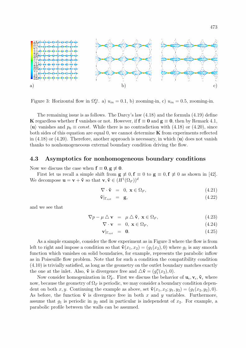
a) b) c)

Figure 3: Horizontal flow in Ωϵ2F . a) uin = 0.1, b) zooming-in, c) uin = 0.5, zooming-in.

The remaining issue is as follows. The Darcy’s law (4.18) and the formula (4.19) defineK regardless whether f vanishes or not. However, if f ≡ 0 and g ≡ 0, then by Remark 4.1,⟨u⟩ vanishes and p0 ≡ const. While there is no contradiction with (4.18) or (4.20), sinceboth sides of this equation are equal 0, we cannot determine K from experiments reflectedin (4.18) or (4.20). Therefore, another approach is necessary, in which ⟨u⟩ does not vanishthanks to nonhomogeneoous external boundary condition driving the flow.

4.3 Asymptotics for nonhomogeneous boundary conditions

Now we discuss the case when f ≡ 0,g ≡ 0.First let us recall a simple shift from g ≡ 0, f ≡ 0 to g ≡ 0, f ≡ 0 as shown in [42].

We decompose u = v + v so that v, v ∈ (H1(ΩF ))d

∇ · v = 0, x ∈ ΩF , (4.21)

v|Γext = g, (4.22)

and we see that

∇p− µ v = µ v, x ∈ ΩF , (4.23)

∇ · v = 0, x ∈ ΩF , (4.24)

v|Γext = 0. (4.25)

As a simple example, consider the flow experiment as in Figure 3 where the flow is fromleft to right and impose a condition so that v(x1, x2) = (g1(x2), 0) where g1 is any smoothfunction which vanishes on solid boundaries, for example, represents the parabolic inflowas in Poiseuille flow problem. Note that for such a condition the compatibility condition(4.10) is trivially satisfied, as long as the geometry on the outlet boundary matches exactlythe one at the inlet. Also, v is divergence free and v = (g′′1(x2), 0).

Now consider homogenization in ΩϵF . First we discuss the behavior of uϵ,vϵ, vϵ where

now, because the geometry of ΩF is periodic, we may consider a boundary condition depen-dent on both x, y. Continuing the example as above, set v(x1, x2; y1, y2) = (g1(x2, y2), 0).As before, the function v is divergence free in both x and y variables. Furthermore,assume that g1 is periodic in y2 and in particular is independent of x2. For example, aparabolic profile between the walls can be assumed.

474

The asymptotic expansions as above now suggest that vϵ and vϵ may have decompo-sitions similar to uϵ, and that, given v0, one could solve the cell-problem for v0

∇yp1 + ∇xp0 − µyy v0 = µyy v0, y ∈ Y, (4.26)

∇y · v0 = 0, y ∈ Y, (4.27)

v0|Γ = 0, (4.28)

v0 periodic in Y. (4.29)

Now notice that v0 satisfies ∇y · v0 = 0. In addition, v0 satisfies the no-slip conditionon Γ. In general we cannot guarantee that v0 is Y -periodic. However, in the special casev(x1, x2; y1, y2) = (g1(y2), 0) with a Y -periodic function g1, this is satisfied. This meansthat u0 = v0 + v0 satisfies

∇yp1 + ∇xp0 − µyy u0 = 0, y ∈ Y, (4.30)

∇y · u0 = 0, y ∈ Y, (4.31)

u0|Γ = 0, (4.32)

u0 periodic in Y. (4.33)

Averaging as proposed in Section 4.2 we obtain that ⟨u0⟩Y = ⟨v0 + v0⟩Y = −K∇xp0. Anextension to Ym and (4.20) is immediate.

We remark that the ansatz proposed here is not the only case in which we obtain ananalogue of (4.20). For example, the use of v which only depends on x would also leadto (4.20).

As for the behavior of p,u, and K for large velocities, the Stokes approximation maynot be valid and neither is its Darcy average. This is discussed in the next section.

4.4 Homogenization for large velocities

For large velocities, we use (2.2) en lieu of (4.7). It must be appropriately scaled asdiscused above:

ϵαuϵ · ∇uϵ + ∇pϵ − ϵ2µ uϵ = f , x ∈ ΩϵF (4.34)

This equation is complemented by (4.8) and (4.9) which together make the Navier-Stokesmodel for flow.

Well-posedness results in [[42], II.1.4 (Theorems 1.5 and 1.6)], while available, dependon the smallness of data f, g, and on a sufficiently large viscosity µ. Additionally, insteadof (4.10), we require that g = ∇× ζ for some smooth function ζ.

Upscaling of the Navier-Stokes model to a nonlinear counterpart of (2.3) known asnon-Darcy model, has been considered in [38], and [23] as well as in several other sources,see references in [2]. The main controversy appears to be as regards the form of theupscaled model. Within homogenization theory, the discussion centers around the scalingα of the advective term in (4.34) and of viscosity term. In particular, [32] suggests to useϵ2 for viscosity which we already included in (4.34). In [[25], Section 3.2.2] additionallyα = 1 which guarantees that the nonlinear corrections do not “disappear” in the processof passing to the limit with ϵ→ 0.

475

Another source of difficulties comes from the boundary conditions. The simple linearshift from nonhomogeneous boundary conditions to nonhomogeneous source term doesnot work for Navier-Stokes system in which a nonlinear term is present. Nevertheless,we apply the same general ideas as in Sections 4.2,4.3 to compute K which now dependson ⟨u⟩Y . Additionally, since the magnitude of ⟨u⟩Y depends on the boundary condition,we consider scaling of g by ϵ. We note that there is a concern that with the scaling ofviscosity, its “large enough” magnitude required for well-posedness is not guaranteed eventhough the scaling via α partially alleviates it.

4.5 Computational experiments

Our considerations will be illustrated with computational results. A synthetic porousmedium at microscale is defined as described above, see Figure 2 b). The distance betweencentres of neighboring circles is d = 0.002[m] and the grain diameter is δ = 0.0019[m],i.e., the radius of grains is 0.00095[m].

As fluid parameters we use ρ = 998.2[kg/m3] and µ = 0.001003[Pa.s], which areproperties of water in standard conditions in a lab. What follows, Re and uin imposedas a boundary condition are linked by Re = 1890, 907uin. For example, uin = 0.001 ;

Re = 1.89. Furthermore, to simulate the homogenization procedure and test whetherthe computational upscaling is stable, we generate a sequence of computational domainsΩϵi

F , i = 1, 2, 3. The reference geometry Ωϵ1F is as in Figure 2 b). To get from Ωϵi

F toΩ

ϵi+1

F , i = 1, 2 we apply a factor 1/2 to the radii of circles. Computations are performedin all domains independently and are denoted as cases ϵ1, ϵ2, and ϵ3.

According to the remark from Section 4.2 we impose scaling of viscosities with a factorϵ2. That is, for ϵ2 we have µ2 = 0.00025075[Pa.s], and µ3 = 0.00006268[Pa.s] for ϵ3.

As opposed to the theoretical presentation of previous sections, where different modelsare applied to describe low and large velocity flows, computations are performed in thesame way for the whole sequence of uin values ranging from 0.00001 to 1, thus coveringlinear and nonlinear flow regimes. In general, more iterations of the numerical solver areneeded for larger velocities.

Figure 3 gives plots of velocity magnitude distribution. Patterns of flow differ in eachflow regime; Figure 3 c) is an illustration of inertia effects.

Now we discuss the results in the context of the homogenization approach. We haveseveral intuitions that we want to verify and confirm. First, as ϵ→ 0, we expect that thepressures and velocities at microscale converge L2-strongly and L2-weakly, respectively, totheir average p0(x) which satisfy Darcy’s law. The convergence of pressures is illustratedin Figure 4; we skip the illustration of velocity convergence, as this would require thecomputation of a corrector. There is a visible difference in pressure shapes obtainedfor low velocity value (uin = 0.1) and large velocities, uin = 0.5 and uin = 1. Similarpressure curves have been reported in [21, 12]. Our experiments confirm the stability ofcomputational laboratory in the homogenization limit.

Second, we expect that K and K can be computed reliably. We use the proceduredescribed in Section 3 to find K (or K) for a range of imposed velocities uin and compareresults obtained for cases ϵ1, ϵ2, and ϵ3.

As is demonstrated in Figure 5 a), K remains essentially constant for a large range of

476

a) b)

c)

Figure 4: Pressure at y = 0 in ΩϵiF , i = 1, 2, 3. a) uin = 0.1, b) uin = 0.5, c) uin = 1.0.

flow rates, moreover, its values obtained for cases ϵ1, ϵ2 and ϵ3 are in a good agreement.Starting from some value of uin we observe the onset of the nonlinear regime, i.e., that Kstarts decreasing with increasing flow rates as predicted by a nonlinear non-Darcy model(2.4). Equivalently the resistance K−1 increases with increasing Re. This qualitativeobservation is fundamental and is consistent with one in upscaling from mesoscale tomacroscale [22]; see also quantitative discussion of K−1 in [34]. Small differences in theasymptotic behavior of K for large velocities are observed.

An interesting result is given in Figure 5 b). We compare K computed for the case ϵ3for different scaling schemes applied to uin and µ. More precisely, we apply 1) scaling µwith the factor ϵ2 as in Section 4.2, or 2) scaling velocity with a factor ϵ1/2 and viscositywith the factor ϵ3/2, or 3) scaling only viscosity with ϵ3/2. For linear regime of flow allthe scalings result in the same value of K; still there are differences in K. This will be asubject of further studies.

Convergence and stability issues related to the upscaling procedure are not addressedin this work; more results are provided in [34].

477

a) b)

Figure 5: Upscaled permeability a) for ΩϵiF , i = 1, 2, 3, no scaling. b) for Ωϵ3

F ; with scalingas follows: 1: ϵ2µ, 2: ϵ3/2µ, ϵ1/2uin, 3: µϵ3/2.

5 Physical experiment

To complete our study and address issue ii) from the Introduction, we compare our com-putational results to the data obtained in the physical experiment reported in [40].

Consider a laboratory stand as given in Figure 6 a). We deal with unconsolidatedporous media composed of granulate of diameter δ = 0.00195[mm]. During the experi-ment, 10 independent measurements of water levels are taken for 12 different values ofvolumetric inflow QV . We calculate mean filtration velocity v = QV /S, where S denotesthe cross-sectional area of a column. The corresponding pressure differences p betweenmeasurements points are computed from water level values. Next we compute absolutepermeability κ, following

κ−1µU = −∇P. (5.35)

More details about the experiment and values of parameters are given in [40].

Now we compare experimental data to the results delivered by the virtual lab experi-ment. First we comment on the parameters of synthetic and experimental porous media.We use δ = 0.0019[mm] and δ = 0.0018[mm] in the former and δ = 0.00195[mm] in thelatter experiment. These are close but not identical. We expect to find similar but notidentical corresponding permeability values.

Next, we discuss scaling between K and κ and flow rates. Since our computationalexperiments delivered K, the values of K−1 in our computational results are multipliedby µ = 0.001003[Pa.s] to get κ−1. Additionally, we shift the computational results tofit measured mean filtration velocities by comparing global water inflow. The combinedcomputational and experimental results are shown in Figure 6.

478

First, we notice the expected qualitative difference between permeabilities computedfor δ = 0.0019[mm] and those for δ = 0.0018[mm]: the conductivities for smaller diametersare larger. Next, we see that the range of velocities covered by the experiment is muchsmaller that the range of velocities used in computations; this is due to the equipmentcapacity, more precisely, to the abilities of rotameter of Figure 6 a) acting in a limited rangeof flow rates. Most importantly, we see a very good qualitative but not perfect quantitativeagreement between computational and experimental conductivities. We believe that theircloseness is quite satisfactory given that they came from uncorrelated experiments. Wealso recall the perspective raised in [6] as concerns poor quality of estimated values of κtypically lying between 1/3 and 3 times the true value. These observations address issueii) raised in Introduction.

In other words, we were able to confirm that the results of the virtual laboratorywere within reasonable accuracy with respect to a physical experiment. In addition,the computational lab did not have the limitations of the experimental setup: we couldperform experiments in any velocity range insofar as the converence and stability of thenumerical scheme could be acertained. Moreover, once the preprocessing i.e. the syntheticporescale geometry is completed, it is relatively inexpensive to obtain data for many flowrates while the cost is linear for experimental results.

We consider these results very encouraging. Taking into account all the simplifica-tions made in our virtual model and poor precision of even good laboratory tests, ourresults compare quite well qualitatively and offer an inexpensive virtual alternative to labexperiments.

6 Conclusions

The computational lab can be applied in order to study Darcy’s law in the transitionfrom linear to nonlinear flow regime. It may also be used in order to study the natureof the Forchheimer coefficient β and its dependence on various factors, see [35, 34]. Weshowed that the virtual lab applies to a range of geometries and in particular thosesuggested by the theory of homogenization. This allows us to find a bridge betweenelegant mathematical theories of homogenization to a more generally applicable theory ofvolume averaging.

In addition we showed that the results of the virtual laboratory were within reasonableaccuracy with respect to the physical experiment. The benefit of such comparison ismultifold. First, the virtual results can be used instead of experimental results. On theother hand, virtual results can be used to guide the set-up of experimental results. Third,once properly callibrated, it could be used to add to the sparse experimental data.

The concept of a computational lab may prove helpful in addressing issues that arehard to handle analytically. More consideration should be given to homogenization forlarge velocities and to appropriate scaling schemes. A systematic study of permeabilitybehavior as a function of synthetic medium geometry, porosity and other parameters forlarge ranges of Re values will be developed in a forthcoming paper.

479

a) b)

Figure 6: a) Scheme of a laboratory stand: a plexi pipe filled with granulate of diameterδ = 0.00195[mm] (6), recharged from the bottom with water, coming from a container (1)through a pump (2). Intensity of inflow is controlled by a valve (3). After passing througha porous bed, water reaches the upper reservoir (7), and then, through the overfall (8)goes down to the bottom reservoir. The flow intensity is measured by a rotameter (5).Pressures are measured by means of U-tube manometers linked to connector pipes (10).b) Measured and computed permeabilities.

Acknowledgements: Peszynska’s research was partially supported from NSF grant0511190 and DOE grant 98089. We used computational facilities at ICM (Sun Constella-tion System with AMD Quad-Core Opteron 835X processors) as well as the facilities atOregon State University including the COE cluster.

References

[1] Robert A. Adams. Sobolev spaces. Academic Press [A subsidiary of Harcourt BraceJovanovich, Publishers], New York-London, 1975. Pure and Applied Mathematics,Vol. 65.

[2] Gregoire Allaire. Mathematical approaches and methods. In Ulrich Hornung, editor,Homogenization and porous media, volume 6 of Interdiscip. Appl. Math., pages 225–250, 259–275. Springer, New York, 1997.

[3] J. S. Andrade, U. M. S. Costa, M. P. Almeida, H. A. Makse, and H. E. Stanley.Inertial effects on fluid flow through disordered porous media. Phys. Rev. Lett.,82(26):5249–5252, Jun 1999.

480

[4] B. Bang and D. Lukkassen. Application of homogenization theory related to Stokesflow in porous media. Applications of Mathematics, 44:309–319, 1999.

[5] G. K. Batchelor. An introduction to fluid dynamics. Cambridge Mathematical Li-brary. Cambridge University Press, Cambridge, paperback edition, 1999.

[6] Jacob Bear. Dynamics of Fluids in Porous Media. Dover, New York, 1972.

[7] Alain Bensoussan, Jacques-Louis Lions, and George Papanicolaou. Asymptotic anal-ysis for periodic structures, volume 5 of Studies in Mathematics and its Applications.North-Holland Publishing Co., Amsterdam, 1978.

[8] B. Biswal, R.J. Held, V. Khanna, J. Wang, and R. Hilfer. Towards precise predictionof transport properties from synthetic computer tomography of reconstructed porousmedia. Physical Review E, 80:041301, 2009.

[9] Zhangxin Chen. Expanded mixed finite element methods for linear second-orderelliptic problems. I. RAIRO Model. Math. Anal. Numer., 32(4):479–499, 1998.

[10] Zhangxin Chen, Stephen L. Lyons, and Guan Qin. Derivation of the Forchheimerlaw via homogenization. Transp. Porous Media, 44(2):325–335, 2001.

[11] K. J. Cho, M.-U. Kim, and H.D. Shin. Linear stability of two–dimensional steadyflow in wavy–walled channels. Fluid Dynamics Research, 23:349–370, 1998.

[12] O. Coulaud, P. Morel, and J.P. Caltagirone. Numerical modelling of nonlinear effectsin laminar flow through a porous medium. J. Fluid. Mech., 190:393–407, 1988.

[13] H. Dong and M.J. Blunt. Pore-network extraction from micro-computerized-tomography images. Physical Review E, 80:036307, 2009.

[14] F.L. Dullien. Porous media. Academic Press San Diego, 1979.

[15] L. J. Durlofsky. Numerical calculation of equivalent grid block permeability tensorsfor heterogeneous porous media. Water Resources Research, 27(5):699–708, 1991.

[16] S. Ergun. Fluid flow through packed columns. Chemical Engineering Progress, 48:89–94, 1952.

[17] Richard E. Ewing, Raytcho D. Lazarov, Steve L. Lyons, Dimitrios V. Papavassiliou,Joseph Pasciak, and Guan Qin. Numerical well model for non-darcy flow throughisotropic porous media. Comput. Geosci., 3(3-4):185–204, 1999.

[18] Fluent Inc. Fluent User’s Guide, ver. 6.3, 2006.

[19] P. Forchheimer. Wasserbewegung durch Boden. Zeit. Ver. Deut. Ing., (45):1781–1788, 1901.

[20] M. Fourar, R. Lenormand, M. Karimi-Fard, and R. Horne. Inertia effects in high-rate flow through heterogeneous porous media. Transport in Porous Media, 60:353–370(18), September 2005.

481

[21] M. Fourar, G. Radilla, R. Lenormand, and C. Moyne. On the non-linear behavior oflaminar single-phase flow through two and three-dimensional porous media. Adv. inWat. Res., 27:669–677, 2004.

[22] C.R. Garibotti and M. Peszynska. Upscaling non-Darcy flow. Transport in PorousMedia, 80:401–430, 2009.

[23] Tiziana Giorgi. Derivation of Forchheimer law via matched asymptotic expansions.Transport in Porous Media, 29:191–206, 1997.

[24] W. Gray and S. Majid Hassanizadeh. High velocity flow in porous media. Transportin porous media, 2:521–531, 1987.

[25] Ulrich Hornung, editor. Homogenization and porous media, volume 6 of Interdisci-plinary Applied Mathematics. Springer-Verlag, New York, 1997.

[26] H. Huang and J. Ayoub. Applicability of the Forchheimer equation for non-Darcyflow in porous media. SPE Journal, (SPE 102715):112–122, March 2008.

[27] Y. Jiao, F.H. Stillinger, and S. Torquato. Modeling heterogeneous materials via two-point correlation functions: basic principles. Physical Review E, 76:031110, 2007.

[28] Guodong Jin, T.W. Patzek, and D.B. Silin. Direct prediction of the absolute perme-ability of unconsolidated and consolidated reservoir rock. SPE 90084, 2004.

[29] M. Karimi-Fard and L.J. Durlofsky. Detailed near-well Darcy-Forchheimer flow mod-eling and upscaling on unstructured 3d grids. SPE 118999, 2009.

[30] S. Mahmud, A.K.M. Sadrul Islam, and M. A. H. Mamun. Separation characteristicsof fluid flow inside two parallel plates with wavy surface. International Journal ofEngineering Science, 40, 2002.

[31] C. C. Mei and J.-L. Auriault. The effect of weak inertia on flow through a porousmedium. J. Fluid Mech., 222:647–663, 1991.

[32] Andro Mikelic. Non-Newtonian flow. In Ulrich Hornung, editor, Homogenization andporous media, volume 6 of Interdiscip. Appl. Math., pages 77–94, 259–275. Springer,New York, 1997.

[33] C. Pan, M. Hilpert, and C.T. Miller. Pore-scale modeling of saturated permeabilitiesin random sphere packings. Physical Review E., 64(066702), 2001.

[34] M. Peszynska and A. Trykozko. Convergence and stability in upscaling of flow withinertia from porescale to mesoscale. accepted to Int. Journal for Multiscale Compu-tational Engineering, December 2009

[35] M. Peszynska, A. Trykozko, and K. Augustson. Computational upscaling of inertiaeffects from porescale to mesoscale. In G. Allen, J. Nabrzyski, E. Seidel, D. vanAlbada, J. Dongarra, and P. Sloot, editors, ICCS 2009 Proceedings, LNCS 5544,Part I, pages 695–704, Berlin-Heidelberg, 2009. Springer-Verlag.

482

[36] M. Peszynska, A. Trykozko, and K. Kennedy. Sensitivity to parameters in non-Darcyflow model from porescale through mesoscale. submitted

[37] P. Renard, and G. de Marsily. Calculating effective permeability: a review. Adv.Water Resour, 20:253–278, 1997.

[38] Enrique Sanchez-Palencia. Nonhomogeneous media and vibration theory, volume 127of Lecture Notes in Physics. Springer-Verlag, Berlin, 1980.

[39] Adrian E. Scheidegger. The physics of flow through porous media. Revised edition.The Macmillan Co., New York, 1960.

[40] W. Sobieski and A. Trykozko. Darcy and Forchheimer laws in experimental andsimulation studies of flow through porous media. in review.

[41] Luc Tartar. Incompressible fluid flow in a porous medium–convergence of the ho-mogenization process. In Nonhomogeneous media and vibration theory, volume 127of Lecture Notes in Physics, pages 368–377. Springer-Verlag, Berlin, 1980.

[42] Roger Temam. Navier-Stokes equations, volume 2 of Studies in Mathematics and itsApplications. North-Holland Publishing Co., Amsterdam, 1979.

[43] Pieter Wesseling. Principles of computational fluid dynamics, volume 29 of SpringerSeries in Computational Mathematics. Springer-Verlag, Berlin, 2001.

[44] Z. Zeng and R. Grigg. A criterion for non-darcy flow in porous media. Transport inPorous Media, 63:57–69, 2006.

[45] Wouter Zijl and Anna Trykozko. Numerical homogenization of the absolute perme-ability using the conformal-nodal and mixed-hybrid finite element method. Transp.Porous Media, 44(1):33–62, 2001.