Full Factorial Design of · PDF fileFull Factorial Design of Experiments. 1 Module Objectives By the end of this module, the participant will: ... • Create and analyze designs in

0

Full Factorial Design of Experiments

1

Module ObjectivesModule Objectives

By the end of this module, the participant will:• Generate a full factorial design• Look for factor interactions• Develop coded orthogonal designs• Write process prediction equations (models) • Set factors for process optimization• Create and analyze designs in MINITAB™

• Evaluate residuals• Develop process models from MINITAB analysis• Determine sample size

2

Why Learn About Full Factorial DOE?Why Learn About Full Factorial DOE?

A Full Factorial Design of Experiment will• Provide the most response information about

– Factor main effects– Factor interactions

• Provide the process model’s coefficients for – All factors– All interactions

• When validated, allow process to be optimized

3

What is a Full Factorial DOEWhat is a Full Factorial DOE

A full factorial DOE is a planned set of tests on the response variable(s) (KPOVs) with one or more inputs (factors) (PIVs) with all combinations of levels–ANOVA analysis will show which factors are significant–Regression analysis will provide the coefficients for the

prediction equations• Mean• Standard deviation

–Residual analysis will show the fit of the model

4

DOE TerminologyDOE Terminology

• Response (Y, KPOV): the process output linked to the Client CTQ

• Factor (X, PIV): uncontrolled or controlled variable whose influence is being studied

• Level: setting of a factor (+, -, 1, -1, hi, lo, alpha, numeric)• Treatment Combination (run): setting of all factors to obtain

a response• Replicate: number of times a treatment combination is run

(usually randomized)• Repeat: non-randomized replicate• Inference Space: operating range of factors under study

5

( , , ...)Y f A B C∧

=

( , , ...)s f A B C∧

=

Full Factorial DOE ObjectivesFull Factorial DOE Objectives

• Learning the most from as few runs as possible.. • Identifying which factors affect mean, variation,

both or have no effect• Modeling the process with prediction equations,

• Optimizing the factor levels for desired response• Validating the results through confirmation

6

Linear Combinations of Factors for Two Levels

7

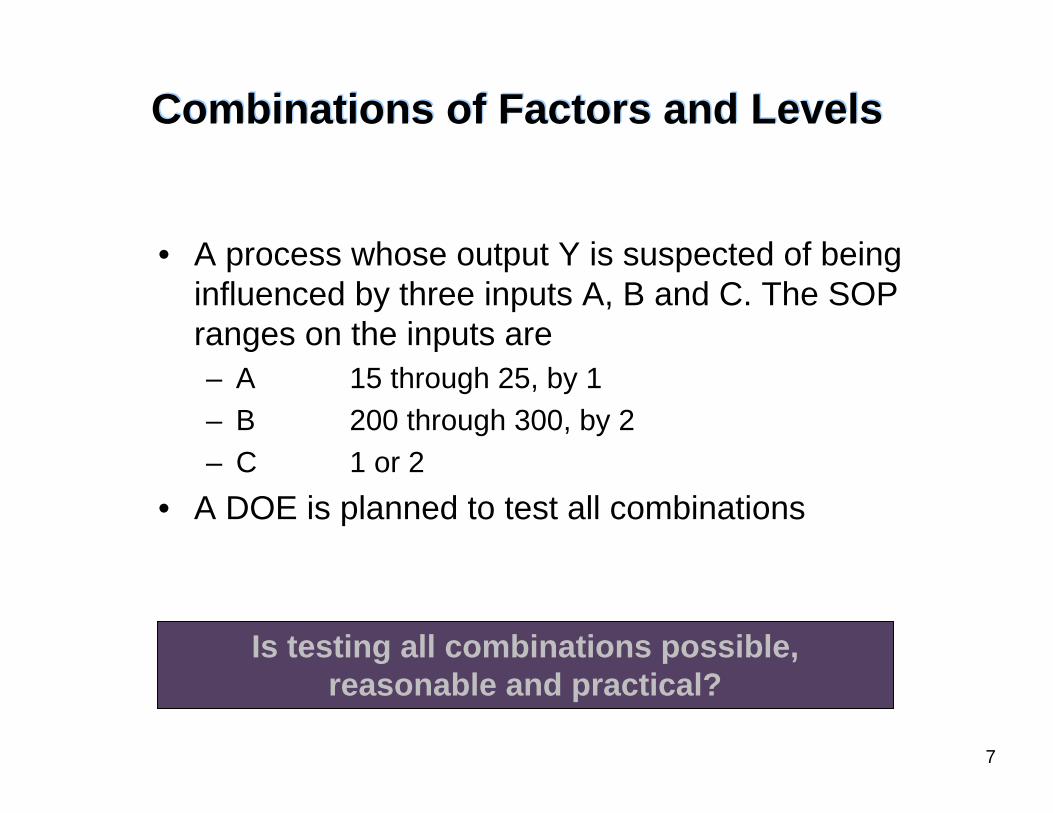
Is testing all combinations possible, reasonable and practical?

Combinations of Factors and LevelsCombinations of Factors and Levels

• A process whose output Y is suspected of being influenced by three inputs A, B and C. The SOP ranges on the inputs are– A 15 through 25, by 1– B 200 through 300, by 2– C 1 or 2

• A DOE is planned to test all combinations

8

We must make assumptions about the response in order to manage the experiment

Combinations of Factors and Levels cont’dCombinations of Factors and Levels cont’d

• Setting up a matrix for the factors at all possible process setting levels will produce a really large number of tests.

• The possible levels for each factor are– A = 11– B = 51– C = 2

• How many combinations are there?

A B C15 200 116 200 117 200 118 200 119 200 120 200 121 200 122 200 123 200 124 200 125 200 115 202 116 202 117 202 1. . .. . .. . .. . .

22 300 223 300 224 300 225 300 2

9

The design becomes much more manageable!

Linear Response for Factors at Two LevelsLinear Response for Factors at Two Levels

• The team decides, from process knowledge, that the response is close to being linear throughout the range of factor level settings (inference space).

• A reasonable assumption for most processes• The levels of the factors for the test would then be

– A 15 and 25– B 200 and 300– C 1 and 2

10

A B C15 200 115 200 215 300 115 300 225 200 125 200 225 300 125 300 2

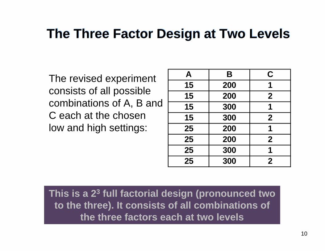
This is a 23 full factorial design (pronounced two to the three). It consists of all combinations of

the three factors each at two levels

The Three Factor Design at Two LevelsThe Three Factor Design at Two Levels

The revised experiment consists of all possible combinations of A, B and C each at the chosen low and high settings:

11

factorlevel

Naming ConventionsNaming Conventions

• The naming convention for full factorial designs has the level raised to the power of the factor:

• And is called “a (level) to the (factor) design”

• What would a two level, four factor design be called?

• How many combinations (runs) are in a 23 design?

12

Write the total number of combinations for the following designs

23

24

Did we all generate the same designs?

Class ExerciseClass Exercise

A B C D

Assume factors are named A, B, C, D, etc. and the levels are low“-” and high “+”.

13

The Yates Standard Order

A method to generate experimental designs in a consistent and logical fashion was

developed by Frank Yates.

14

Runs A B C12345678

Factors

For a 23

there will be 8 runs

The Yates Standard Order: Step 1The Yates Standard Order: Step 1

Create a matrix with factors along the top, runs down the left side (23 example shown)

15

Runs A B C1 152 253 154 255 156 257 158 25

Factors


Starting with the first factor, insert its low value in the first row followed by its high value in the second row. Repeat through the last row.

16

Runs A B C1 15 2002 25 2003 15 3004 25 3005 15 2006 25 2007 15 3008 25 300

Factors


Move to the next factor and place its low value in the first two rows, followed by its high value in the next two rows. Repeat through the last row.

17

Runs A B C1 15 200 12 25 200 13 15 300 14 25 300 15 15 200 26 25 200 27 15 300 28 25 300 2

Factors


Move to the next factor and place its low value in the first four rows, followed by its high value in the next four rows. Repeat through the last row.

18

The Yates Standard Order: Step NThe Yates Standard Order: Step N

Continue the pattern until all factors are included• Yates Design Generator

– Factor Row Pattern– 1st 1 low, 1 high– 2nd 2 low, 2 high– 3rd 4 low, 4 high

– nth 2n-1 low, 2n-1 high

19

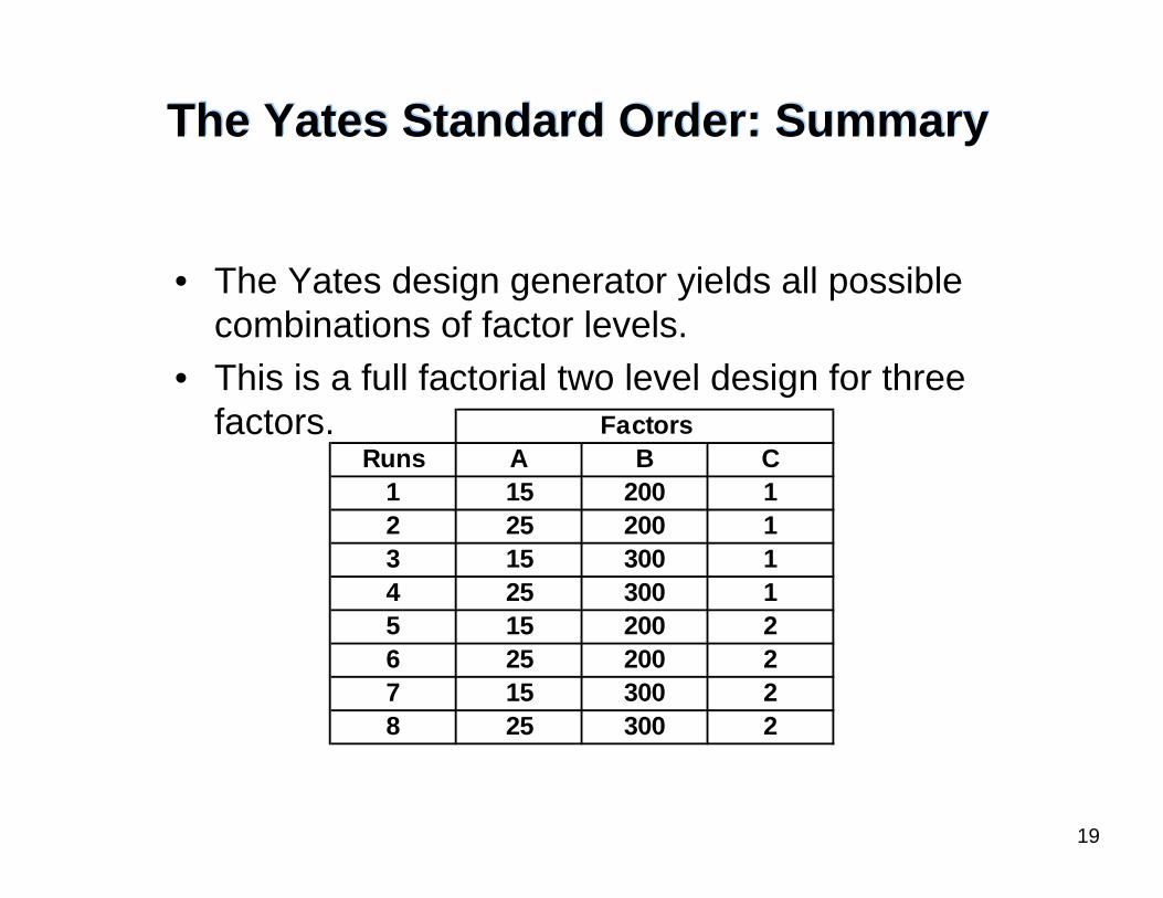
The Yates Standard Order: SummaryThe Yates Standard Order: Summary

• The Yates design generator yields all possible combinations of factor levels.

• This is a full factorial two level design for three factors.

Runs A B C1 15 200 12 25 200 13 15 300 14 25 300 15 15 200 26 25 200 27 15 300 28 25 300 2

Factors

20

Class ExerciseClass Exercise

• Write the total number of combinations for the following designs using the Yates Standard order design generator.– 23

– 24

• Assume factors are named A, B, C, D, etc. and the levels are low = “-” and high =“+”.

Did we all generate the same designs?

21

This is the Yates Standard order for a 23

uncoded design

Creating a Factorial Design in MINITABCreating a Factorial Design in MINITAB

22

StdOrder Column of MINITAB DesignStdOrder Column of MINITAB Design

The StdOrder Column is the Yates Standard Order

23

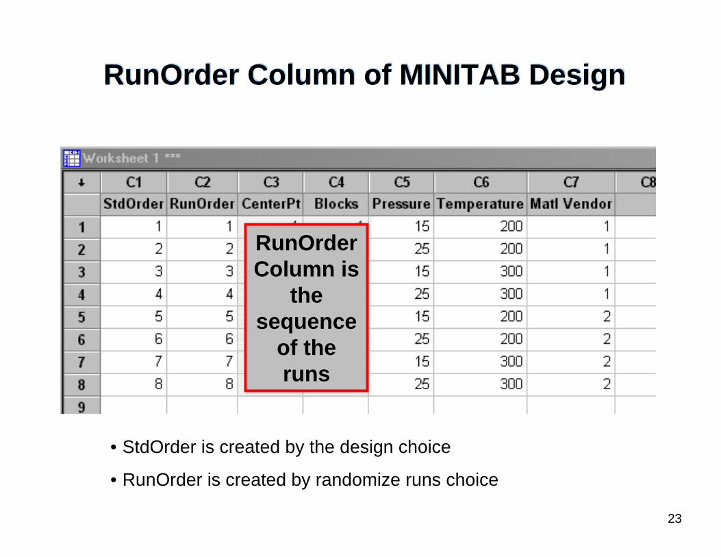
RunOrder Column of MINITAB DesignRunOrder Column of MINITAB Design

RunOrder Column is

the sequence

of the runs

• StdOrder is created by the design choice

• RunOrder is created by randomize runs choice

24

Replicates and Repeats

25

What are Replicates and Repeats?What are Replicates and Repeats?

Replicate• Total run of all treatment combinations

– Usually in random order• Requires factor level change between runs• All experiments will have one replicate

– Two replicates are two complete experiment runs• Statistically best experimental scenario• Repeat (also repetition)• Additional run without factor level change

26

MINITAB Design ReplicationMINITAB Design Replication

MINITAB easily handles replicating the design• Replicate or repeat is treated same in design• Actual factor level change between runs is at the

discretion of the experimenter– MINITAB provides treatment combination– Randomization or information needed is part of

strategy of experiment

27

Replication in MINITAB Step 1 Replication in MINITAB Step 1

Create a 22 with two non randomized replicatesTool Bar Menu > Stat > DOE > Factorial > Create Factorial Design

28


29


Skip the other dialog options

Un-check randomize box in Options

30


First Replicate

Second Replicate

Response Y would be placed in C7

31

Randomized Replication in MINITAB for Step 4

Response Y would be placed in C7

32

Coding the Design

Coding the design by transforming the low factor level to a “-1” and the high factor

level to a “+1” offers analysis advantages

33

Any uncoded design can be transformed into a coded design

Runs A B C A B C1 15 200 12 25 200 13 15 300 14 25 300 15 15 200 26 25 200 27 15 300 28 25 300 2

Uncoded Factors Coded Factors

Coding Review ExerciseCoding Review Exercise

Fill in the coded design based upon the uncoded design

34

Coded to Uncoded TransferCoded to Uncoded Transfer

• The transfer from coded to uncoded values is

• where– Hi = the uncoded high level– Low = the uncoded low level

2 2uncoded codedHi Lo Hi LoX X+ −

= +

35

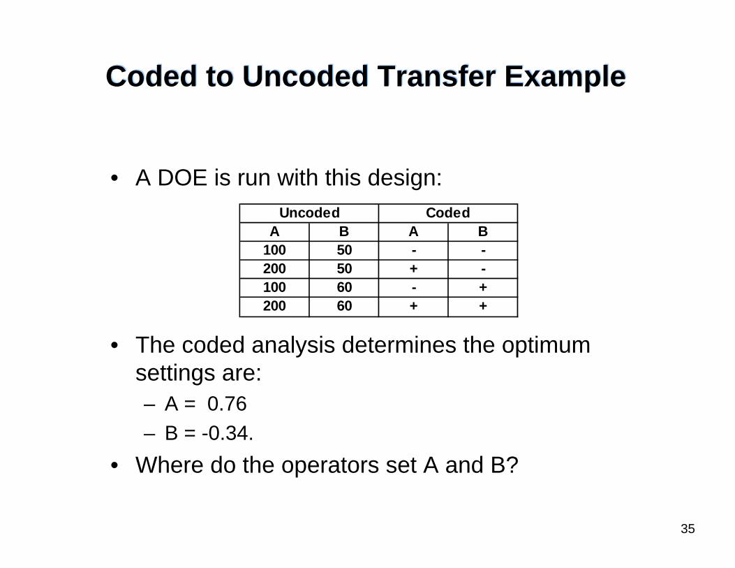
Coded to Uncoded Transfer ExampleCoded to Uncoded Transfer Example

• A DOE is run with this design:

• The coded analysis determines the optimum settings are: – A = 0.76 – B = -0.34.

• Where do the operators set A and B?

A B A B100 50 - -200 50 + -100 60 - +200 60 + +

Uncoded Coded

36

Converting A Uncoded Factor SettingsConverting A Uncoded Factor Settings

200 100 200 1000.76

2 2uncodedA+ −

= +

150 0.76*50

188

uncoded

uncoded

A

A

= +

=

2 2uncoded codedH i Lo Hi LoX X+ −

= +

Remembering

for Acoded = 0.76

37

Converting B Uncoded Factor SettingsConverting B Uncoded Factor Settings

60 50 60 50( 0.34)

2 2uncodedB+ −

= + −

55 0.34*5

53.3

uncoded

uncoded

B

B

= −

=

2 2uncoded codedH i Lo Hi LoX X+ −

= +

Remembering

for Bcoded = -0.34

38

Class Coding Transfer ExerciseClass Coding Transfer Exercise

• The optimum coded settings from a 23 DOE show the significant factors should be set to– A = 0.43C = -0.87

• Where do you tell your operators to set the real world process values?

• Be prepared to present your results.

O2 flow lpm A 43.6 61.6

Au Slurry lb/hr B 0.01 15Mandrel rpm C 91 142

Factor Label

SOP LOW

SOP HIGH

Process Input Units

39

Requirement of Factor IndependenceRequirement of Factor Independence

Factors are mathematically independent when only the response is a function of the factors–A factor is not a function of another factor–The coded design is orthogonal –Factors will be independent

DOE analysis requires that the factors be independent

40

Orthogonal Designs

41

Determining OrthogonalityDetermining Orthogonality

OutPutRuns X1 X2 Y

1 -1 -1 (y1)2 1 -1 (y2)3 -1 1 (y3)4 1 1 (y4)

Coded FactorsConsider the 22

design

The run outputs, Yn, can be described by

1 2n n nY b X c X= + where b and c are coded settings of the factors

It can be shown that for X1to be independent of X2

10

n

i ii

b c=

=∑

42

Calculating OrthogonalityCalculating Orthogonality

Coef1*coeff2Runs X1 X2 X1*X2

1 -1 -1 12 1 -1 -13 -1 1 -14 1 1 1

Σ 0

Coded Factors

Satisfies1

0n

i ii

b c=

=∑ Therefore orthogonal and independent

43

Orthogonality ExerciseOrthogonality Exercise

Verify the orthogonality of a 23 full factorial design.

Runs X1 X2 X3 X1X2 X1X3 X2X31 -1 -1 -12 1 -1 -13 -1 1 -14 1 1 -15 -1 -1 16 1 -1 17 -1 1 18 1 1 1

Σ

Coded Factors Prod of Factor Settings

44

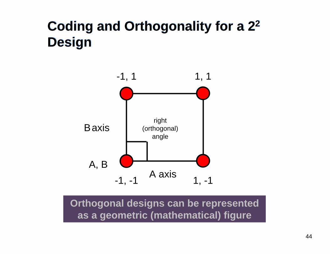
Orthogonal designs can be represented as a geometric (mathematical) figure

Coding and Orthogonality for a 22

DesignCoding and Orthogonality for a 22

Design

right (orthogonal)

angle

A axis

Baxis

-1, -1

-1, 1 1, 1

1, -1A, B

45

Coding and Orthogonality for a 23

DesignCoding and Orthogonality for a 23

Design

A

BC

-1,1,1

1,1,-1-1,1,-1

1,1,1

-1,-1, 1 1,-1,1

1,-1,-1-1,-1,-1

The vertices are the response measurement points; the volume within is the inference space

46

A

B

-1, -1

-1, 1 1, 1

1, -1

Y(-1,-1)

Y(-1, 1) Y(1, 1)

Y(1, -1)

Response and OrthogonalityResponse and Orthogonality

The response can be measured at each corner of the design, as represented by Y(A,B).

47

Since the factors are orthogonal, Y is a linear combination of each factor

Fitting a linear model to the coded design becomes very easy

Coding and the Linear ModelCoding and the Linear Model

The linear equation,

describes the line between the points

0 1Y b b A= +

1b =Rise/Run0b = Intercept

-1 1YA

0b Rise

Run

48

Main Effects and Interactions

49

A DOE is run:

The factor (or main) effects are easily calculated

(@ ) (@ )effect Y factorhigh Y factorlow= −

ResponseA B Y-1 -1 481 -1 96-1 1 721 1 36

Yave at FACTORhigh 66 54Yave at FACTORlow 60 72

Effect 6 -18

Coded Factors

What does a non-zero effect

mean?

Calculating Main EffectsCalculating Main Effects

96 36 662+

=

50

A response change due to both A and B changing is called an interaction

Discovering InteractionsDiscovering Interactions

ResponseA B Y-1 -1 481 -1 96-1 1 721 1 36

Coded Factors

51

1 30 2Y b b A ABb bB∧

= + + +

Linear Prediction Equation With Interaction TermLinear Prediction Equation With Interaction Term

• The interaction will add a term to the linear equation

• A and B are the main effects• AB is the interaction• b0 is the grand mean (intercept)• b1, b2, and b3 are the term coefficients

52

Finding the interaction levels in a coded design is as simple as multiplying one times one

A B-1 -11 -1-1 11 1

AB1-1-11

-1*-1 = 11*-1 = -1-1*1 = -11*1 = 1

Coded Values for InteractionsCoded Values for Interactions

The coded value matrix for an interaction is the product of the factor coded values:

53

The interaction is set by the design (math) based upon the factor settings

Interaction ResponseA B AB Y-1 -1 1 481 -1 -1 96-1 1 -1 721 1 1 36

Yave at FACTORhigh 66 54 42Yave at FACTORlow 60 72 84

Effect 6 -18 -42

Coded Factors

Calculating Interaction EffectsCalculating Interaction Effects

The DOE again• This is the Yates Standard Order for a 22 coded

design with interaction

54

Main Effects, Interactions and Cube Plots in MINITAB

55

Input the Y response

Create the ExperimentCreate the Experiment

Create a 22 coded design for factors A and B.

56

Select the type of factorial plot

desired

Select the response column and the factor columns

Similarly setup interaction and

cube plots

Factorial Plots in MINITAB: Step 1Factorial Plots in MINITAB: Step 1

57

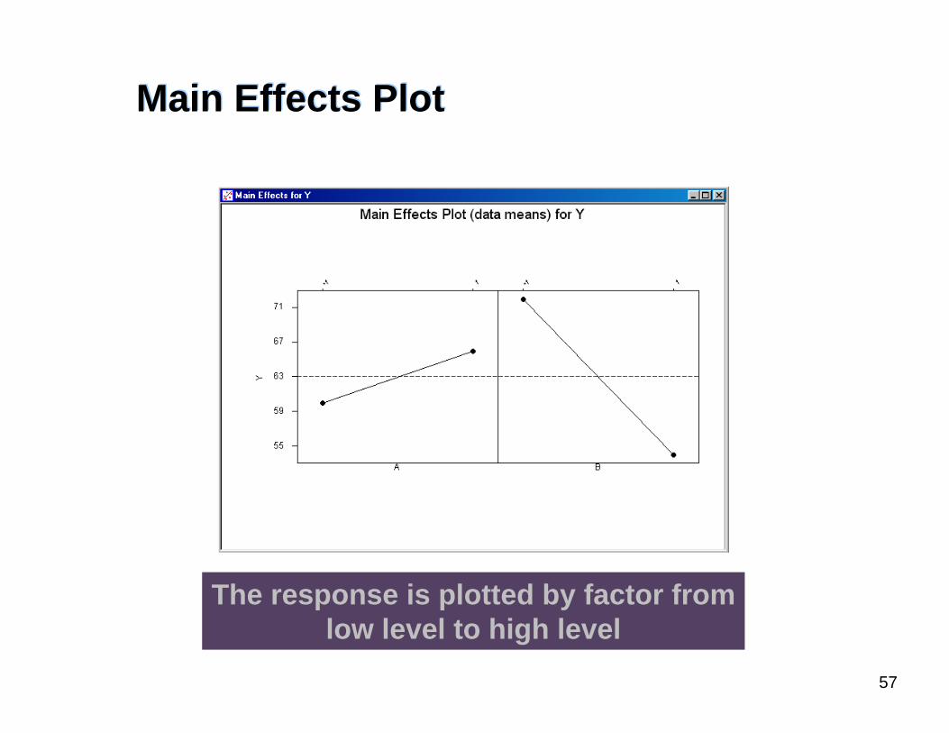
The response is plotted by factor from low level to high level

Main Effects PlotMain Effects Plot

58

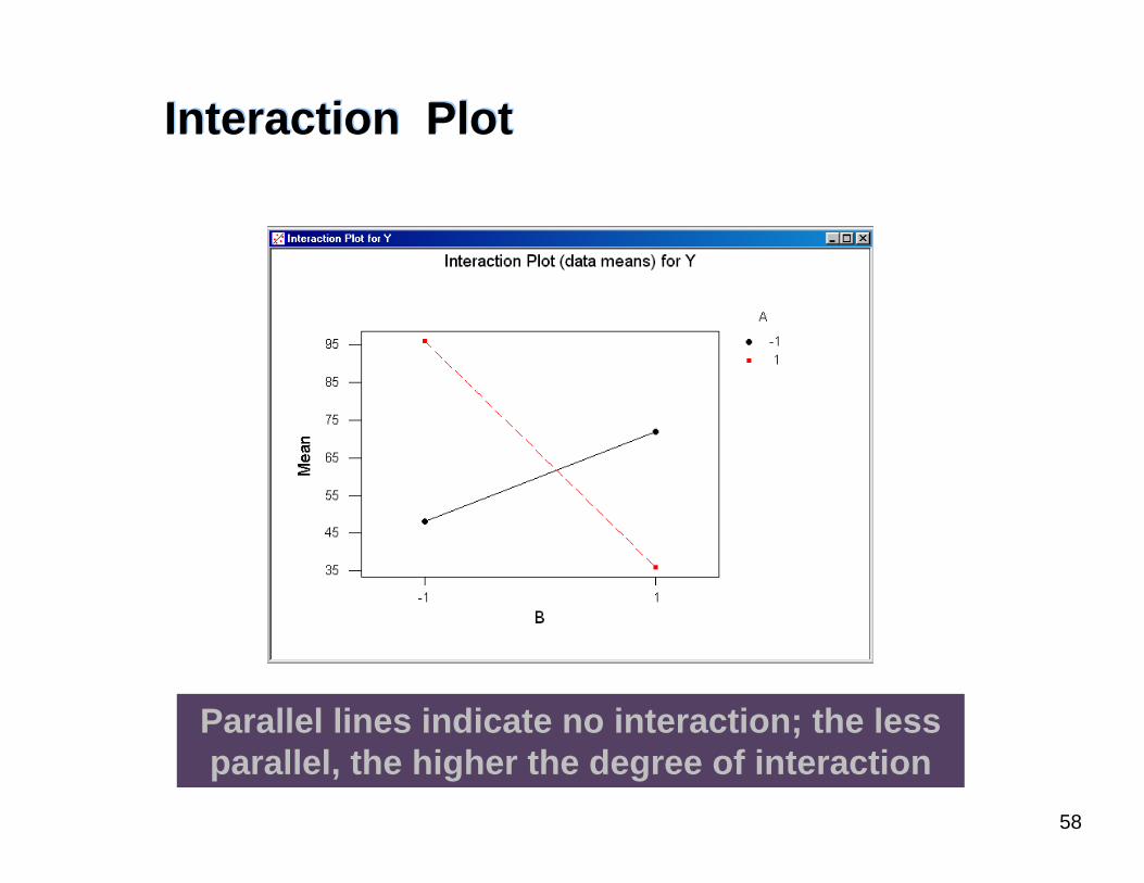
Parallel lines indicate no interaction; the less parallel, the higher the degree of interaction

Interaction PlotInteraction Plot

59

The response is plotted on the orthogonal factor axis

Cube PlotCube Plot

60

The Prediction Equations

61

0 1 2 3Y b b A b B b AB∧

= + + +

Developing the Prediction EquationDeveloping the Prediction Equation

Knowing the design, responses and effect analysis the prediction equation can be found.


Yave at FACTORhigh 66 54 42Yave at FACTORlow 60 72 84

Effect 6 -18 -42

Coded Factors

62

0 1 2 3Y b b A b B b AB∧

= + + +

0Y b∧

=

The regression constant is the grand mean of the responses for a coded design

The Intercept – Constant – Grand Mean RelationshipThe Intercept – Constant – Grand Mean Relationship

• If we set all (coded) factors to equal zero, the equation becomes:

• which is the overall average, or grand mean. The grand mean of the response is 63.

63

1 2 363Y b A b B b AB∧

= + + +

Looking at in coded units 1b Awhen A = 1, Yave = 66and when A = -1, Yave = 60

The rise from –1 to +1 is 6 The run is 2The slope is 6/2 = 3

The regression coefficients are the factor effects divided by two for a coded design

Finding the CoefficientsFinding the Coefficients

-1 1

Y@(A= -1)

Y@(A= 1)

YA

y

64

Verify the equation for the coded A and B values in the matrix


Yave at FACTORhigh 66 54 42 Grand Mean 63Yave at FACTORlow 60 72 84

Effect 6 -18 -42Coefficient 3 -9 -21

Coded Factors

63 3 9 21Y A B AB∧

= + − −

Finishing the MatrixFinishing the Matrix

65

Interaction Response Std DevA B A B AB Y1, Y2, ...Yn Yaverage s

200 15 48 7.36300 15 96 7.36200 25 72 3.96300 25 36 3.96

Grand Mean

Coded Factors

Yave at FACTORhigh

Yave at FACTORlow

Uncoded Factors

s Effects Coefficient

Y EffectY Coefficient

s at FACTORhigh

s at FACTORlow

Where would you set the factors to minimize Y and s?

Class Model Building ExerciseClass Model Building Exercise

Given the following designed experiment and responses, determine the prediction equation for Y and s

66

DOE Analysis in MINITAB

67

Input the Y response

Create the ExperimentCreate the Experiment

Create or recall the 22 coded design for factors A and B.

68

Select the Y response

Go to terms menu

Setting Up the AnalysisSetting Up the Analysis

Tool Bar Menu > Stat > DOE > Factorial > Analyze Factorial Design

69

Select all of the available

terms

note the AB interaction!

Selecting TermsSelecting Terms

70

The coefficients are identical to manual analysis

The AnalysisThe Analysis

71

Select the Y

responseGo to terms menu

Another AnalysisAnother Analysis

Recalling the exercise fileTool Bar Menu > Stat > DOE > Factorial > Analyze Factorial Design

72

Select all of the

available terms

note interaction

terms

What can be estimated with this model? How many terms in the prediction equation?

Setting Up the AnalysisSetting Up the Analysis

73

From the Graphs menu

select the graphs shown

Selecting Graph OptionsSelecting Graph Options

74

The ANOVA Table shows temperature and pressure are significant; regression coefficients are listed

The ANOVA ResultsThe ANOVA Results

75

Normality Plot and Histogram of the

residuals show the residuals to be “normal”

Residuals can also stored in the worksheet for

normality testing

The Graph ResultsThe Graph Results

76

Looking for random distributions without a

pattern

The residual vs. fits show slight widening, but the widening here is

not a concern; look for strong outliers and patterns that could

indicate special cause

The Residuals GraphsThe Residuals Graphs

77

The Pareto of effects shows the ranking of the variation identified by each source; note the “line of significance”

Where did the axis values come from?

The Pareto of Standardized EffectsThe Pareto of Standardized Effects

78

The ANOVA table coefficients column feeds the

prediction equation

0 1 2 3 4 5 6 7Y b b A b B b C b AB b AC b BC b ABC∧

= + + + + + + +

The ANOVA table p-value column identifies the significant effects, or terms of the regression; to simplify the prediction

equation the number of terms must be reduced

The Prediction Equation from MINITABThe Prediction Equation from MINITAB

79

Remove insignificant terms

Removing Model Terms in MINITABRemoving Model Terms in MINITAB

80

Removing Terms StepwiseRemoving Terms Stepwise

When reducing the regression model do not remove all insignificant terms at once–Removed terms variance go into error, along with their

degrees of freedom–Significance levels can change as terms are removed–Start with higher order terms and remove no more than

two at a time –Run analysis and check for changes in significance

81

Compare the significant terms Adj MS with the residual error; the error should be less than 20% of the total variation

0.664 0.061 0.026Y A B∧

= − −

Where do you set the factors to optimize this process?

Re-run Reduced Model in MINITABRe-run Reduced Model in MINITAB

82

Sample Size in MINITAB

83

Input the values

Power and Sample Size in MINITAB Step 1Power and Sample Size in MINITAB Step 1

Set up risk

Solving for replicates

Tool Bar Menu > Stat > Power and Sample Size > 2 Level Factorial Design

84

Power and Sample Size in MINITAB Step 2Power and Sample Size in MINITAB Step 2

Optional worksheet storage

85

To detect an effect difference of 3, two replicates must be taken

Power and Sample Size in MINITABPower and Sample Size in MINITAB

86

Class Sample Size ExerciseClass Sample Size Exercise

• You are running a 2 level four factor design trying to see a difference of 1.4 hours. The standard deviation is 1.1 hours. Accepting an α risk of 0.05 and a β risk of 0.10, how many replicates do you need?

• Be prepared to show your results.

87

The General Linear Model

88

Why GLM?Why GLM?

The General Linear Model • Allows more flexible design• Allows multiple levels• Does not require factors to have same number of

levels• Is well suited for business process problems

89

Setting up a GLM DesignSetting up a GLM Design

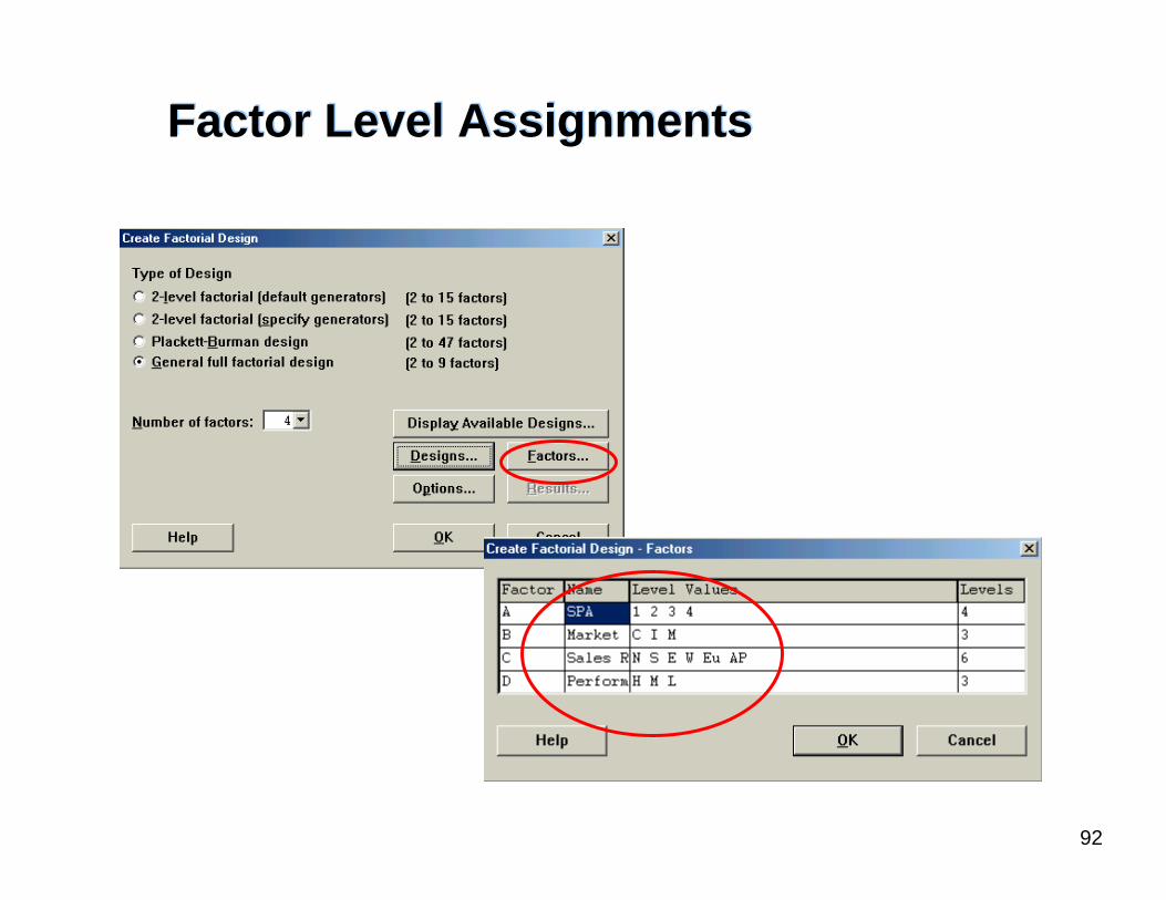
• Account receivables lockup, where payments are withheld, is thought to be caused by four factors– SPAs (Special Pricing Agreements) -4 categories– Market sector – 3 demographics– Sales region – 6 regional centers– Performance to contract – 3 levels

• Design a DOE to study the problem

90

Setting up GLMSetting up GLM

Tool Bar Menu > Stat > DOE > Factorial > Create Factorial Design

91

Factor Name and Number of Level AssignmentsFactor Name and Number of Level Assignments

92

Factor Level AssignmentsFactor Level Assignments

93

Options Options

94

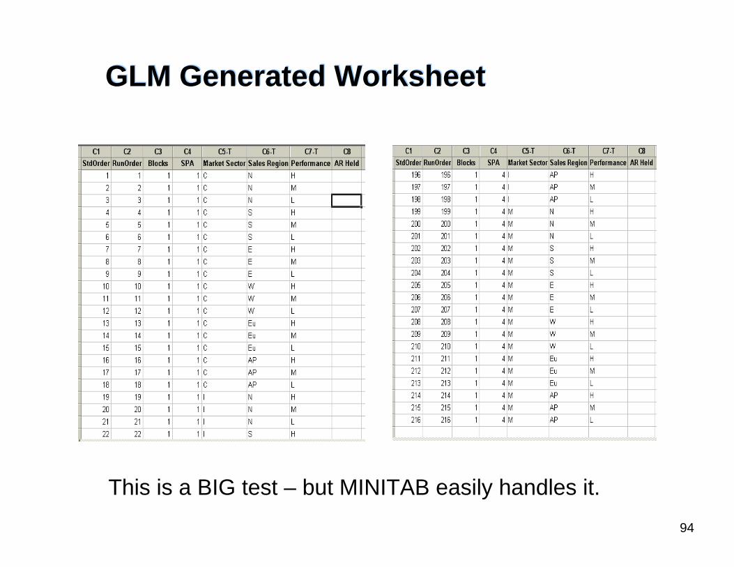
GLM Generated WorksheetGLM Generated Worksheet

This is a BIG test – but MINITAB easily handles it.

95

Objectives ReviewObjectives Review

By the end of this module, the participant should:• Generate a full factorial design• Look for factor interactions• Develop coded orthogonal designs• Write process prediction equations (models) • Set factors for process optimization• Create and analyze designs in MINITAB• Evaluate residuals• Develop process models from MINITAB analysis• Determine sample size

Documents

Full Factorial Design of · PDF fileFull Factorial Design of Experiments. 1 Module Objectives By the end of this module, the participant will: ... • Create and analyze designs in