Generation scheduling technologies supporting large ... i it j i it F Pu j w C P u S u u 1 1 1 1 ( , ) ( , ) ( ) ( , ) 2 : Fuelconsunp tio n function i it j i j it i j i C P u a P

© Hitachi, Ltd. 2016. All rights reserved.

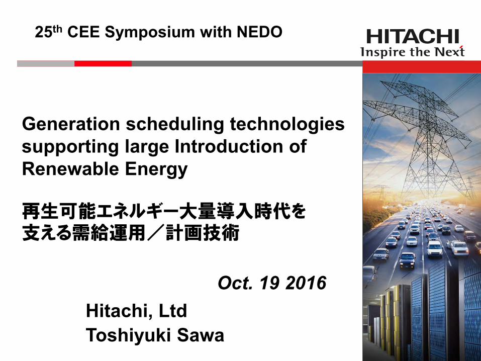
再生可能エネルギー大量導入時代を支える需給運用／計画技術

Oct. 19 2016 Hitachi, Ltd Toshiyuki Sawa

Generation scheduling technologies supporting large Introduction of Renewable Energy

25th CEE Symposium with NEDO


Contents

1. Backgrounds and Objectives 2. Overview of methods for Uncertainties 3. UC method using Quadratic Programming 4. Proposed method for Uncertainties 5. Results 6. Conclusions & Future works


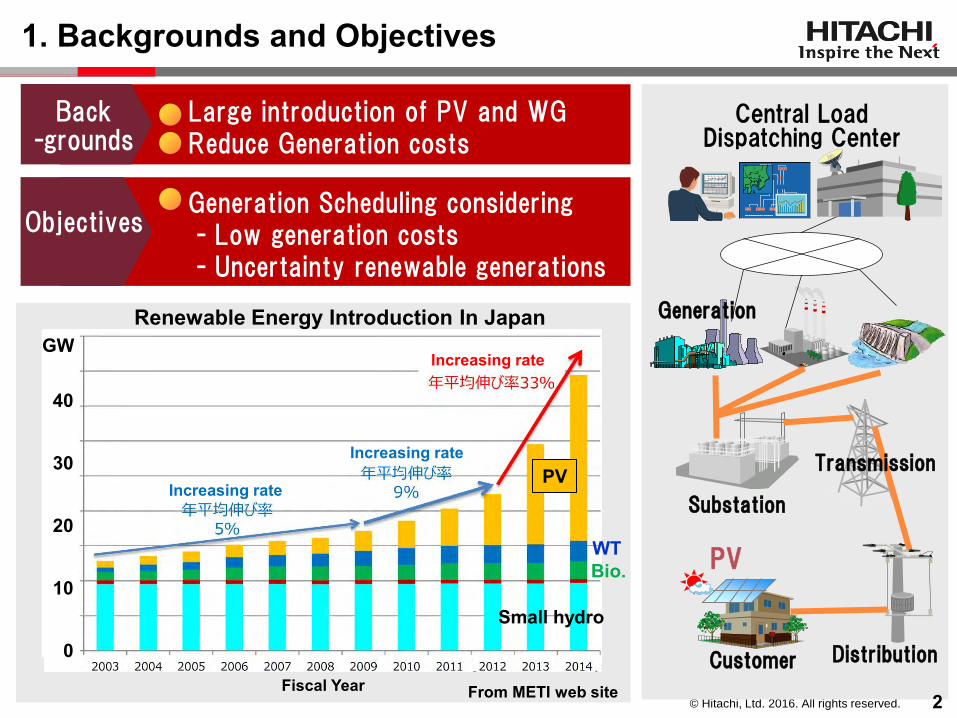
Large introduction of PV and WG Reduce Generation costs

1. Backgrounds and Objectives

Central Load Dispatching Center

Generation

Substation

Transmission

Distribution Customer

PV

Back -grounds

Generation Scheduling considering - Low generation costs - Uncertainty renewable generations

Objectives

Fiscal Year

10

0

20

30

40

GW

Increasing rate

Increasing rate

Increasing rate

PV

WT Bio.

Small hydro

Renewable Energy Introduction In Japan

From METI web site 2


Contents


© Hitachi, Ltd. 2016. All rights reserved. 4

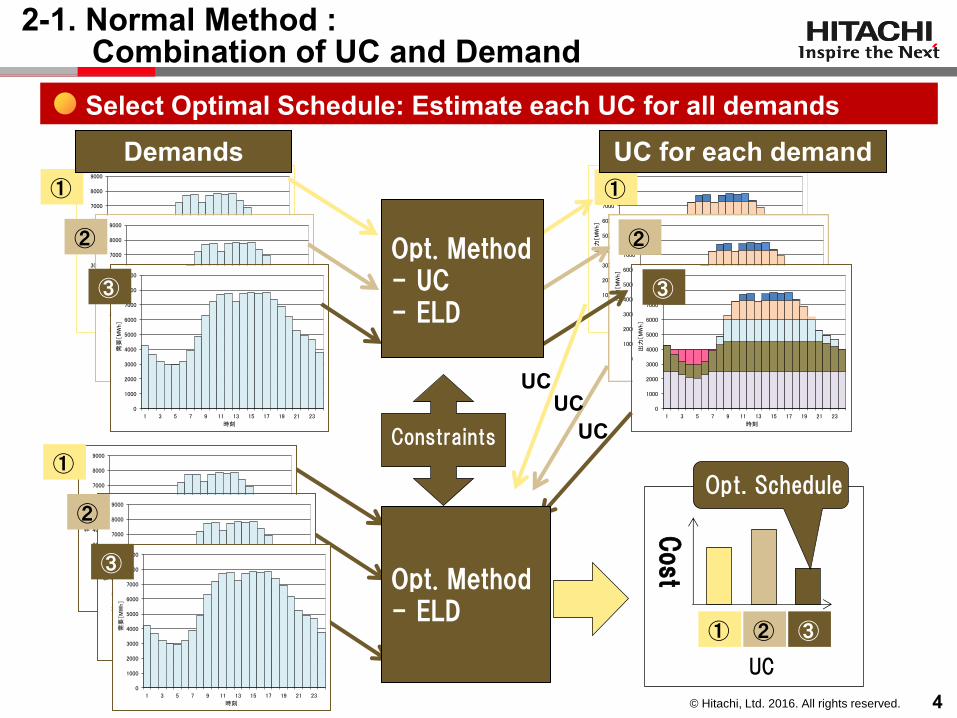
2-1. Normal Method : Combination of UC and Demand

0

1000

2000

3000

4000

5000

6000

7000

8000

9000

1 3 5 7 9 11 13 15 17 19 21 23

需要

［M

Wh］

時刻

0

1000

2000

3000

4000

5000

6000

7000

8000

9000

1 3 5 7 9 11 13 15 17 19 21 23

出力

［M

Wh］

時刻

0

1000

2000

3000

4000

5000

6000

7000

8000

9000

1 3 5 7 9 11 13 15 17 19 21 23

需要

［M

Wh］

時刻

0

1000

2000

3000

4000

5000

6000

7000

8000

9000

1 3 5 7 9 11 13 15 17 19 21 23

需要

［M

Wh］

時刻

0

1000

2000

3000

4000

5000

6000

7000

8000

9000

1 3 5 7 9 11 13 15 17 19 21 23

出力

［M

Wh］

時刻

0

1000

2000

3000

4000

5000

6000

7000

8000

9000

1 3 5 7 9 11 13 15 17 19 21 23

出力

［M

Wh］

時刻UC

①

②

③

Opt. Method - UC - ELD

Constraints

UC UC

UC for each demand Select Optimal Schedule: Estimate each UC for all demands

Opt. Method - ELD

0

1000

2000

3000

4000

5000

6000

7000

8000

9000

1 3 5 7 9 11 13 15 17 19 21 23

需要

［M

Wh］

時刻

0

1000

2000

3000

4000

5000

6000

7000

8000

9000

1 3 5 7 9 11 13 15 17 19 21 23

需要

［M

Wh］

時刻

UC

Cost

① ② ③

0

1000

2000

3000

4000

5000

6000

7000

8000

9000

1 3 5 7 9 11 13 15 17 19 21 23

需要

［M

Wh］

時刻

Opt. Schedule

①

②

③

Demands

①

②

③

© Hitachi, Ltd. 2016. All rights reserved. 5

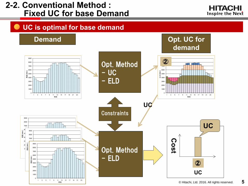
2-2. Conventional Method : Fixed UC for base Demand

0

1000

2000

3000

4000

5000

6000

7000

8000

9000

1 3 5 7 9 11 13 15 17 19 21 23

需要

［M

Wh］

時刻

0

1000

2000

3000

4000

5000

6000

7000

8000

9000

1 3 5 7 9 11 13 15 17 19 21 23

出力

［M

Wh］

時刻

②

0

1000

2000

3000

4000

5000

6000

7000

8000

9000

1 3 5 7 9 11 13 15 17 19 21 23

需要

［M

Wh］

時刻

0

1000

2000

3000

4000

5000

6000

7000

8000

9000

1 3 5 7 9 11 13 15 17 19 21 23

需要

［M

Wh］

時刻

0

1000

2000

3000

4000

5000

6000

7000

8000

9000

1 3 5 7 9 11 13 15 17 19 21 23

需要

［M

Wh］

時刻

UC

Cost

②

UC

UC

Demand Opt. UC for demand

UC is optimal for base demand

Opt. Method - UC - ELD

Constraints

Opt. Method - ELD


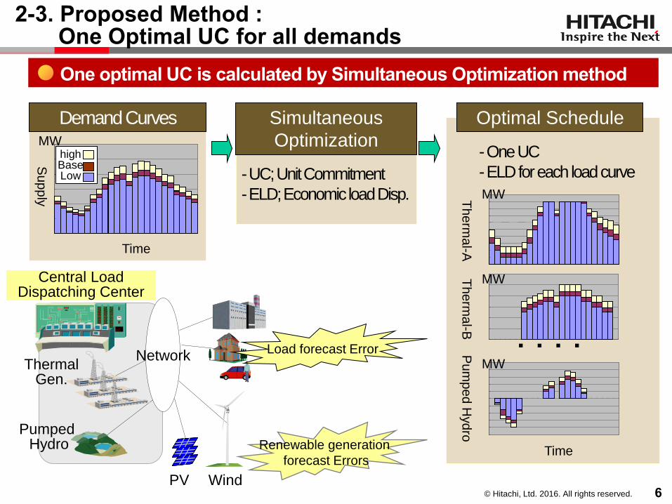
2-3. Proposed Method : One Optimal UC for all demands

Thermal Gen.

Pumped Hydro Renewable generation

forecast Errors

Wind

Load forecast Error

Supply

時間 Time

Th

erm

al-A

T

he

rma

l-B

Pu

mp

ed

Hyd

ro

Time

・・・・

- One UC

- ELD for each load curve

Network

PV

high Base Low

Demand Curves Optimal Schedule

- UC; Unit Commitment

- ELD; Economic load Disp.

Simultaneous

Optimization

Central Load Dispatching Center

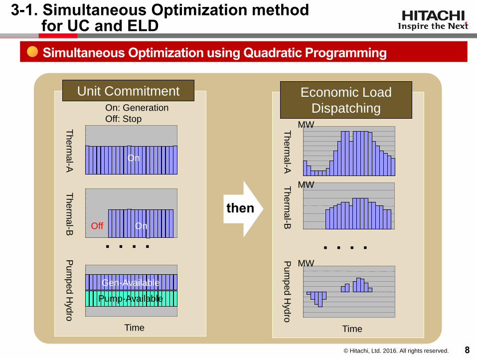
One optimal UC is calculated by Simultaneous Optimization method

MW

MW

MW

MW

6


Contents



3-1. Simultaneous Optimization method for UC and ELD

時間

Th

erm

al-A

T

he

rma

l-B

Pu

mp

ed

Hyd

ro

Time

・・・・

Economic Load

Dispatching

Pu

mp

ed

Hyd

ro

Time

・・・・

Unit Commitment

時間

Th

erm

al-A

時間

Th

erm

al-B

On

On Off

Gen-Available

Pump-Available

MW

MW

MW

On: Generation

Off: Stop

then

Simultaneous Optimization using Quadratic Programming

8


3-2. Formulation for Integrated Unit Commitment

N

i

ii

T

t

N

i

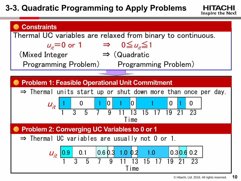
ititi SCuPCuPF11 1

)(),(),(

itiitiitiiti ucPbPaPC 2

)( iiii SvSC )(

Thermal UC Variable uit 0≦uit≦1 relaxing binary to continuous Increasing UC Variable uit≦uit+1 when demand increasing Decreasing UC Variable uit≧uit+1 when demand decreasing

Fuel Cost Start-up Cost

- Generation Capacity and minimum generation - System demand and supply balance - Spinning Reserve - Minimum up and down times - Transmission Constraints - LNG Consumption - Hydro unit power, load limit and reservoir water level

・・・(1) Mixed integer programming problem

↓ Quadratic programming problem

Objective Function：Generation Costs → min

Newly added Constraints

Main constraints

9


3-3. Quadratic Programming to Apply Problems

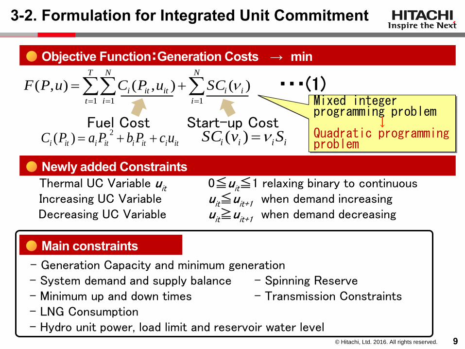
Problem 1: Feasible Operational Unit Commitment ⇒ Thermal units start up or shut down more than once per day.

Problem 2: Converging UC Variables to 0 or 1 ⇒ Thermal UC variables are usually not 0 or 1.

Thermal UC variables are relaxed from binary to continuous. uit＝0 or １ ⇒ 0≦uit≦1 （Mixed Integer ⇒ （Quadratic Programming Problem） Programming Problem）

1 3 5 7 9 11 13 15 17 19 21 23 Time

uit 1 0 0 0 1 1 0 1 0 1

1 3 5 7 9 11 13 15 17 19 21 23 Time

uit 0.9 0.1 0.6 0.3 1.0 0.2 1.0 0.3 0.6 0.2

Constraints

Problem 1: Feasible Operational Unit Commitment

Problem 2: Converging UC Variables to 0 or 1

10


3-4. Measure against Problem 1

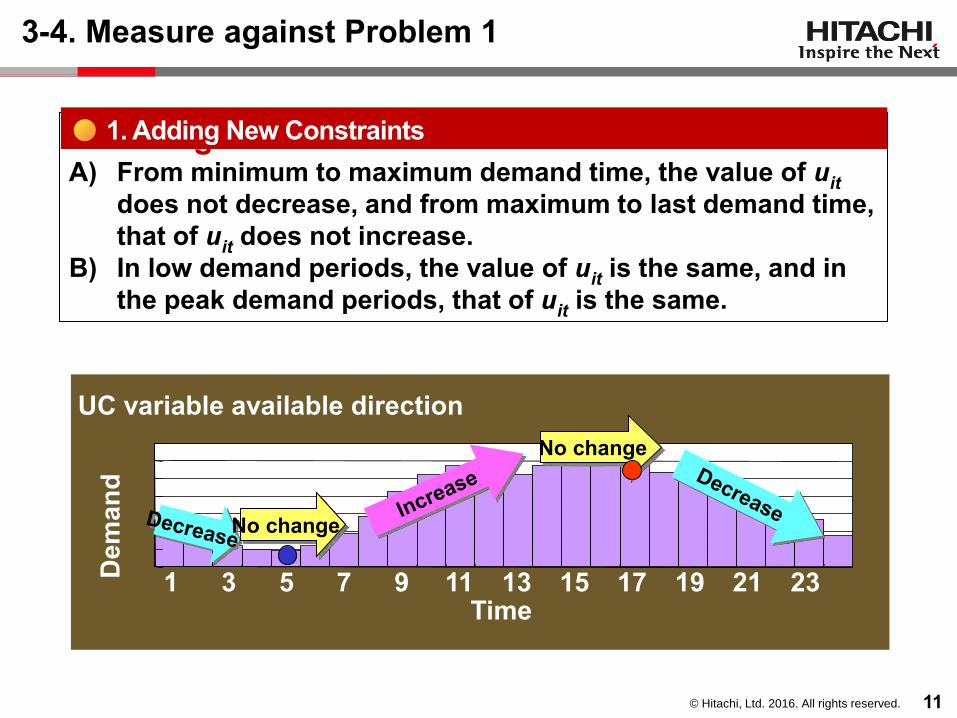
1. Adding New Constraints A) From minimum to maximum demand time, the value of uit

does not decrease, and from maximum to last demand time, that of uit does not increase.

B) In low demand periods, the value of uit is the same, and in the peak demand periods, that of uit is the same.

1 3 5 7 9 11 13 15 17 19 21 23 Time

Dem

and

No change

No change

UC variable available direction

1. Adding New Constraints

11


3-5. Measure against Problem 2

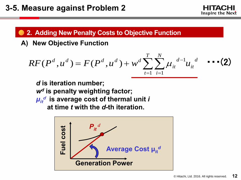
A) New Objective Function

Average Cost μitd

Generation Power

Pitｄ

Fuel

cos

t

T

t

N

i

d

it

d

it

ddddd uwuPFuPRF1 1

1),(),(

d is iteration number; wd is penalty weighting factor; μiｔ

ｄ is average cost of thermal unit i at time t with the d-th iteration.

・・・(2)

2. Adding New Penalty Costs to Objective Function

12


3-6. Flowchart for generation scheduling

Yes

No

Calculate dispatching power and unit commitment using QP in Eq. 29

Calculate initial dispatching power and unit commitment using QP in Eq. 29 （d=0, wd=0,）

d=d+1, wd＝10d

Calculate per-unit fuel cost μ itk

at present dispatching power Pitd

k>kmax ?

Calculate dispatching power using QP in Eq. 1

Decide unit commitmentif uit

d >0 then uit=1(committed) else uit=0

Output final generation schedule

d > dmax ?

Yes

No

Calculate dispatching power and unit commitment using QP in Eq. 29

Calculate initial dispatching power and unit commitment using QP in Eq. 29 （d=0, wd=0,）

d=d+1, wd＝10d

Calculate per-unit fuel cost μ itk

at present dispatching power Pitd

k>kmax ?

Calculate dispatching power using QP in Eq. 1

Decide unit commitmentif uit

d >0 then uit=1(committed) else uit=0

Output final generation schedule

d > dmax ?

d

it

13


Contents



4-1. Mathematical Formation for generation scheduling （１）目的関数：発電コスト＝燃料費＋起動費最小化

・・・・・・・・・・・・ (1)

（２）制約条件

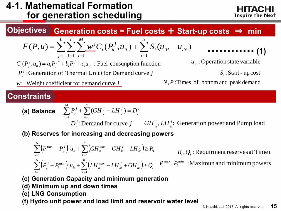
(a) Balance (b) Reserves for increasing and decreasing powers (c) Generation Capacity and minimum generation (d) Minimum up and down times (e) LNG Consumption (f) Hydro unit power and load limit and reservoir water level

N

i

iNiPi

L

j

T

t

M

i

it

j

iti

j uuSuPCwuPF11 1 1

)(),(),(

functionn consunptio Fuel:),(2

iti

j

i

j

iit

j

i ucPbPauPCititit

jiP j

itcurve Demandfor UnitThermal of Generation:

variablestateOperation:itu

costupStart: iS

jw j curve demandfor t coefficienWeight : demandpeak and bottom of Times:, PN

jjK

k

jM

i

j

tktktitDLHGHP

)(11

jD j

t curvefor Demand: load Pump andpower Generation：, jj

ktktLHGH

t

K

k

j

kt

j

ktkit

N

i

j

i RLHGHGHuPPit

1

max

1

max

t

K

k

j

kt

j

ktkit

N

i

i

j QGHLHLHuPPit

1

max

1

min powersminimum andMaximun:, minmax 　ii PP

tQR tt TimeatreservesRequirment:,

Generation costs = Fuel costs ＋ Start-up costs ⇒ min Objectives

Constraints

15


4-2. Conditions of Scheduling Problem

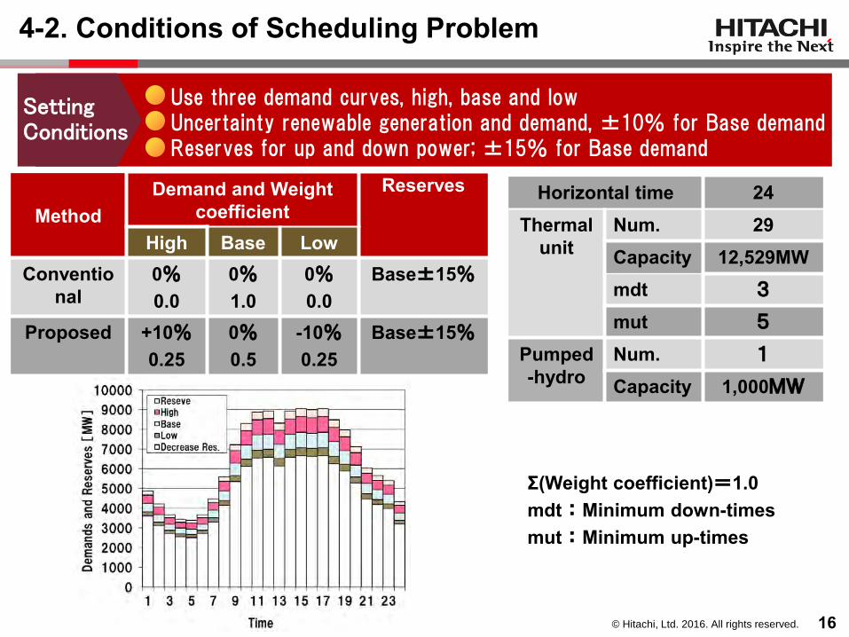
Horizontal time 24 Thermal

unit Num. 29 Capacity 12,529MW mdt ３ mut ５

Pumped-hydro

Num. １ Capacity 1,000ＭＷ

Method Demand and Weight

coefficient Reserves

High Base Low Conventio

nal 0％ 0.0

0％ 1.0

0％ 0.0

Base±15％

Proposed +10％ 0.25

0％ 0.5

-10％ 0.25

Base±15％

Σ(Weight coefficient)＝1.0 mdt ： Minimum down-times mut ： Minimum up-times

Use three demand curves, high, base and low Uncertainty renewable generation and demand, ±10％ for Base demand Reserves for up and down power; ±15％ for Base demand

Setting Conditions

16


Contents



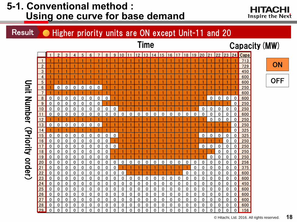
5-1. Conventional method : Using one curve for base demand

Unit N

um

ber

（Priority o

rder

）

時間 1 2 3 4 5 6 7 8 9 10 11 12 13 14 15 16 17 18 19 20 21 22 23 24 容量

1 1 1 1 1 1 1 1 1 1 1 1 1 1 1 1 1 1 1 1 1 1 1 1 1 7132 1 1 1 1 1 1 1 1 1 1 1 1 1 1 1 1 1 1 1 1 1 1 1 1 7293 1 1 1 1 1 1 1 1 1 1 1 1 1 1 1 1 1 1 1 1 1 1 1 1 4504 1 1 1 1 1 1 1 1 1 1 1 1 1 1 1 1 1 1 1 1 1 1 1 1 6005 1 1 1 1 1 1 1 1 1 1 1 1 1 1 1 1 1 1 1 1 1 1 1 1 6006 1 0 0 0 0 0 0 1 1 1 1 1 1 1 1 1 1 1 1 1 1 1 1 1 2507 1 1 1 1 1 1 1 1 1 1 1 1 1 1 1 1 1 1 1 1 1 1 1 1 6008 0 0 0 0 0 0 0 0 1 1 1 1 1 1 1 1 1 1 1 1 0 0 0 0 6009 0 0 0 0 0 0 0 1 1 1 1 1 1 1 1 1 1 1 1 1 1 1 1 0 250

10 0 0 0 0 0 0 0 0 0 1 1 1 1 1 1 1 1 1 1 0 0 0 0 0 25011 0 0 0 0 0 0 0 0 0 0 0 0 0 0 0 0 0 0 0 0 0 0 0 0 60012 1 1 1 1 1 1 1 1 1 1 1 1 1 1 1 1 1 1 1 1 0 0 0 0 25013 0 0 0 0 0 0 0 1 1 1 1 1 1 1 1 1 1 1 1 1 1 1 1 0 25014 1 1 1 1 1 1 1 1 1 1 1 1 1 1 1 1 1 1 1 1 1 1 1 0 32515 0 0 0 0 0 0 0 0 0 1 1 1 1 1 1 1 1 1 1 0 0 0 0 0 32516 0 0 0 0 0 0 0 0 1 1 1 1 1 1 1 1 1 1 1 1 1 1 0 0 25017 0 0 0 0 0 0 0 0 0 1 1 1 1 1 1 1 1 1 1 0 0 0 0 0 25018 0 0 0 0 0 0 0 0 1 1 1 1 1 1 1 1 1 1 1 1 1 0 0 0 25019 0 0 0 0 0 0 0 0 1 1 1 1 1 1 1 1 1 1 1 1 0 0 0 0 25020 0 0 0 0 0 0 0 0 0 0 0 0 0 0 0 0 0 0 0 0 0 0 0 0 25621 0 0 0 0 0 0 0 0 0 1 1 1 1 1 1 1 1 1 0 0 0 0 0 0 37522 0 0 0 0 0 0 0 0 0 0 1 1 1 1 1 1 1 0 0 0 0 0 0 0 60023 0 0 0 0 0 0 0 0 0 0 0 0 0 0 0 0 0 0 0 0 0 0 0 0 60024 0 0 0 0 0 0 0 0 0 0 0 0 0 0 0 0 0 0 0 0 0 0 0 0 45025 0 0 0 0 0 0 0 0 0 0 0 0 0 0 0 0 0 0 0 0 0 0 0 0 60026 0 0 0 0 0 0 0 0 0 0 0 0 0 0 0 0 0 0 0 0 0 0 0 0 60027 0 0 0 0 0 0 0 0 0 0 0 0 0 0 0 0 0 0 0 0 0 0 0 0 60028 0 0 0 0 0 0 0 0 0 0 0 0 0 0 0 0 0 0 0 0 0 0 0 0 60029 0 0 0 0 0 0 0 0 0 0 0 0 0 0 0 0 0 0 0 0 0 0 0 0 156

Time

ON

OFF

Higher priority units are ON except Unit-11 and 20 Result

Capacity(MW) Capa

18


5-2. Proposed method : Simultaneous Optimization method using three demand curves

時間 1 2 3 4 5 6 7 8 9 10 11 12 13 14 15 16 17 18 19 20 21 22 23 24 容量

1 1 1 1 1 1 1 1 1 1 1 1 1 1 1 1 1 1 1 1 1 1 1 1 1 7132 1 1 1 1 1 1 1 1 1 1 1 1 1 1 1 1 1 1 1 1 1 1 1 1 7293 1 1 1 1 1 1 1 1 1 1 1 1 1 1 1 1 1 1 1 1 1 1 1 1 4504 1 1 1 1 1 1 1 1 1 1 1 1 1 1 1 1 1 1 1 1 1 1 1 1 600

5 1 1 1 1 1 1 1 1 1 1 1 1 1 1 1 1 1 1 1 1 1 1 1 1 6006 0 0 0 0 0 0 0 0 0 1 1 1 1 1 1 1 1 1 1 1 0 0 0 0 2507 1 1 1 1 1 1 1 1 1 1 1 1 1 1 1 1 1 1 1 1 1 1 1 1 6008 0 0 0 0 0 0 0 0 1 1 1 1 1 1 1 1 1 1 1 0 0 0 0 0 6009 1 0 0 0 0 0 0 1 1 1 1 1 1 1 1 1 1 1 1 1 1 1 1 1 250

10 0 0 0 0 0 0 0 0 0 1 1 1 1 1 1 1 1 1 1 1 0 0 0 0 25011 1 1 1 1 1 1 1 1 1 1 1 1 1 1 1 1 1 1 1 1 1 1 1 0 60012 0 0 0 0 0 0 0 0 1 1 1 1 1 1 1 1 1 1 1 1 0 0 0 0 25013 0 0 0 0 0 0 0 1 1 1 1 1 1 1 1 1 1 1 1 1 1 0 0 0 25014 1 1 1 1 1 1 1 1 1 1 1 1 1 1 1 1 1 1 1 1 1 1 1 1 32515 0 0 0 0 0 0 0 1 1 1 1 1 1 1 1 1 1 1 1 1 1 1 1 0 32516 0 0 0 0 0 0 0 0 1 1 1 1 1 1 1 1 1 1 1 1 1 1 0 0 25017 0 0 0 0 0 0 0 0 0 0 0 0 0 0 0 0 0 0 0 0 0 0 0 0 25018 0 0 0 0 0 0 0 0 0 1 1 1 1 1 1 1 1 1 0 0 0 0 0 0 25019 1 0 0 0 0 0 1 1 1 1 1 1 1 1 1 1 1 1 1 1 1 1 1 1 25020 0 0 0 0 0 0 0 0 0 0 0 1 1 1 1 1 1 0 0 0 0 0 0 0 25621 0 0 0 0 0 0 0 0 0 0 1 1 1 1 1 1 1 0 0 0 0 0 0 0 37522 0 0 0 0 0 0 0 0 0 0 0 0 0 0 0 0 0 0 0 0 0 0 0 0 60023 0 0 0 0 0 0 0 0 0 0 0 0 0 0 0 0 0 0 0 0 0 0 0 0 600

24 0 0 0 0 0 0 0 0 0 0 0 0 0 0 0 0 0 0 0 0 0 0 0 0 45025 0 0 0 0 0 0 0 0 0 0 0 0 0 0 0 0 0 0 0 0 0 0 0 0 600

26 0 0 0 0 0 0 0 0 0 0 0 0 0 0 0 0 0 0 0 0 0 0 0 0 60027 0 0 0 0 0 0 0 0 0 0 0 0 0 0 0 0 0 0 0 0 0 0 0 0 60028 0 0 0 0 0 0 0 0 0 0 0 0 0 0 0 0 0 0 0 0 0 0 0 0 60029 0 0 0 0 0 0 0 0 0 0 0 0 0 0 0 0 0 0 0 0 0 0 0 0 156

Higher priority units are ON except Unit-17 Result

Unit N

um

ber

（Priority o

rder

）

Time

ON

OFF

Capacity(MW) Capa

19


5-3. Differences of Unit commitments

1 2 3 4 5 6 7 8 9 10 11 12 13 14 15 16 17 18 19 20 21 22 23 24 容量

6 0 0 0 0 0 0 0 0 0 1 1 1 1 1 1 1 1 1 1 1 0 0 0 0 2507 1 1 1 1 1 1 1 1 1 1 1 1 1 1 1 1 1 1 1 1 1 1 1 1 6008 0 0 0 0 0 0 0 0 1 1 1 1 1 1 1 1 1 1 1 0 0 0 0 0 6009 1 0 0 0 0 0 0 1 1 1 1 1 1 1 1 1 1 1 1 1 1 1 1 1 250

10 0 0 0 0 0 0 0 0 0 1 1 1 1 1 1 1 1 1 1 1 0 0 0 0 25011 1 1 1 1 1 1 1 1 1 1 1 1 1 1 1 1 1 1 1 1 1 1 1 0 60012 0 0 0 0 0 0 0 0 1 1 1 1 1 1 1 1 1 1 1 1 0 0 0 0 25013 0 0 0 0 0 0 0 1 1 1 1 1 1 1 1 1 1 1 1 1 1 0 0 0 25014 1 1 1 1 1 1 1 1 1 1 1 1 1 1 1 1 1 1 1 1 1 1 1 1 32515 0 0 0 0 0 0 0 1 1 1 1 1 1 1 1 1 1 1 1 1 1 1 1 0 32516 0 0 0 0 0 0 0 0 1 1 1 1 1 1 1 1 1 1 1 1 1 1 0 0 25017 0 0 0 0 0 0 0 0 0 0 0 0 0 0 0 0 0 0 0 0 0 0 0 0 25018 0 0 0 0 0 0 0 0 0 1 1 1 1 1 1 1 1 1 0 0 0 0 0 0 25019 1 0 0 0 0 0 1 1 1 1 1 1 1 1 1 1 1 1 1 1 1 1 1 1 25020 0 0 0 0 0 0 0 0 0 0 0 1 1 1 1 1 1 0 0 0 0 0 0 0 25621 0 0 0 0 0 0 0 0 0 0 1 1 1 1 1 1 1 0 0 0 0 0 0 0 37522 0 0 0 0 0 0 0 0 0 0 0 0 0 0 0 0 0 0 0 0 0 0 0 0 600

Unit N

um

ber

（Priority o

rder

）

Time

ON by only Proposed method

Capacity(MW)

ON by only Conventional method

600MW Unit-11 ON 250MW Unit-12 ON

Bottom Peak

600MW-11+256MW-20 Units ON 600MW-22+250MW-17 Units ON

Proposed Conventional

Differences of UC are one and two units in bottom and peak times respectively Other differences are start-up and shut-down time

Difference

Capa

20


5-4. Results : In case of high demand, base + 10％

① All constraints are satisfied in case of 15 % reserve for base demand.

② Final water level ＜ Target level Power[kW]can balance at each time but not energy[kWh]

③ Compensation costs are added to raise target water level Average unit cost × ΔWater Level [k¥/kWh] [kWh]

0

500

1000

1500

2000

2500

1 3 5 7 9 11 13 15 17 19 21 23

予備力[

M

W

ｈ]

時刻

揚水火力

0

500

1000

1500

2000

2500

1 3 5 7 9 11 13 15 17 19 21 23

予備力[

M

W

ｈ]

時刻

揚水火力

Proposed ① Satisfy all constraints

Conventional ② Violation of Water level

③ Lower than target Level

Time

Time

Res

erve

(M

W)

Res

erve

(M

W)

Pump Therm

Pump Therm

Thermal Units P

um

pe

d

Pu

mp

ed

21


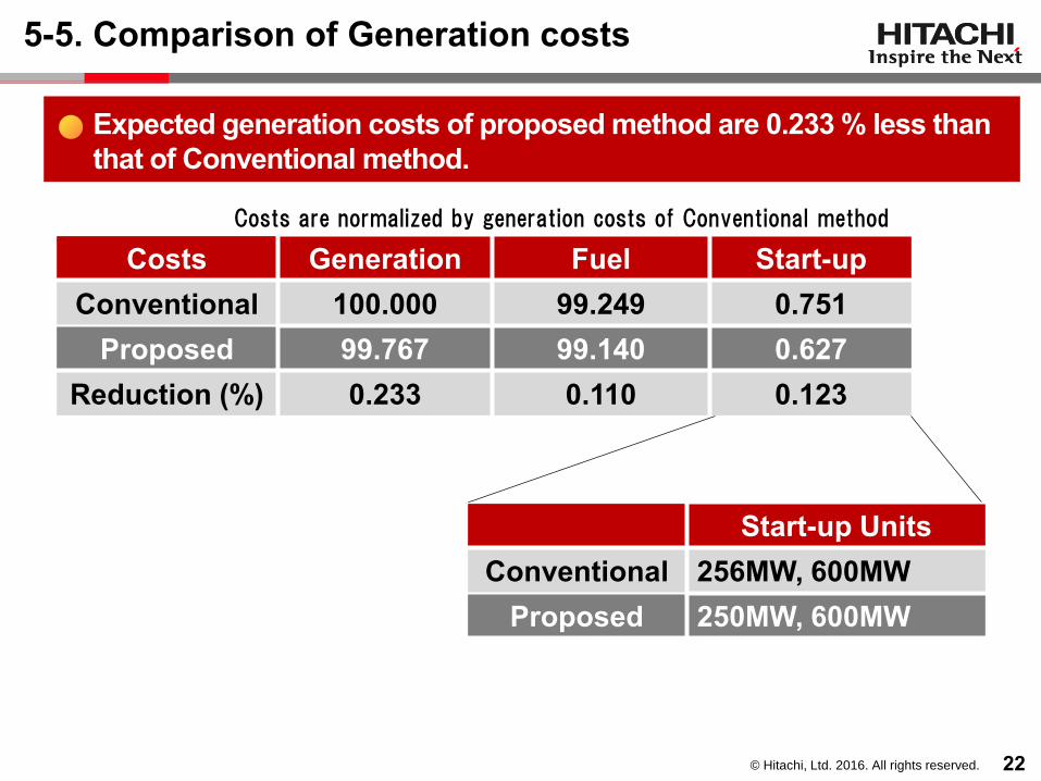
5-5. Comparison of Generation costs

Costs Generation Fuel Start-up Conventional 100.000 99.249 0.751

Proposed 99.767 99.140 0.627 Reduction (%) 0.233 0.110 0.123

Costs are normalized by generation costs of Conventional method

Start-up Units Conventional 256MW, 600MW

Proposed 250MW, 600MW

Expected generation costs of proposed method are 0.233 % less than that of Conventional method.

22


Contents



6-1. Conclusions

Generation Scheduling method has been developed for uncertainties such as large introduction of renewable energy. - Using Quadratic Programming - Solving simultaneously UC and ELD Simulation results from proposed method show - Satisfy all constraints - Reduce generation costs by 0.233%. Pumped-hydro as energy storage system is important for uncertainties to keep not only kW-power balance but also kWh-energy balance.

24


6-2. Future works

Simulate and estimate more realistic cases considering - Uncertainties for each time dependent - Network constraints

25

Thank you for your kind attention!

Documents

Generation scheduling technologies supporting large ... i it j i it F Pu j w C P u S u u 1 1 1 1 ( , ) ( , ) ( ) ( , ) 2 : Fuelconsunp tio n function i it j i j it i j i C P u a P