Embed Size (px)
Citation preview
Genetic Algorithms for
multiple resource constraints
Production Scheduling with multiple levels of product structure
By : Pupong Pongcharoen (Ph.D. Research Student)
Supervisors : Prof. Paul Braiden
Dr. Chris Hicks
26 April 1999
Dept. of MMME, University of Newcastle upon Tyne
Overview of this presentation
Background and literature review Characteristics of production scheduling
problem Optimisation algorithms Genetic Algorithms(GAs) applied to production
scheduling Experimental Program Results Discussions and conclusions
What is scheduling ?
“ The allocation of resources over time to perform a collection of tasks ”
“ Scheduling problems in their simple static and deterministic forms are extremely simple to describe and formulate but difficult to solve ”
Baker(1974)
King and Spackis(1980)
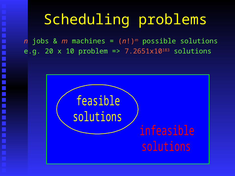
Scheduling problems
n jobs & m machines = (n!)m possible solutions
e.g. 20 x 10 problem => 7.2651x10183 solutions
feasiblesolutions
infeasiblesolutions
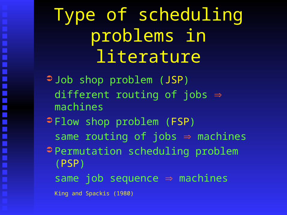
Type of scheduling problems in literature
Job shop problem (JSP)
different routing of jobs machines Flow shop problem (FSP)
same routing of jobs machines Permutation scheduling problem (PSP)
same job sequence machinesKing and Spackis
(1980)
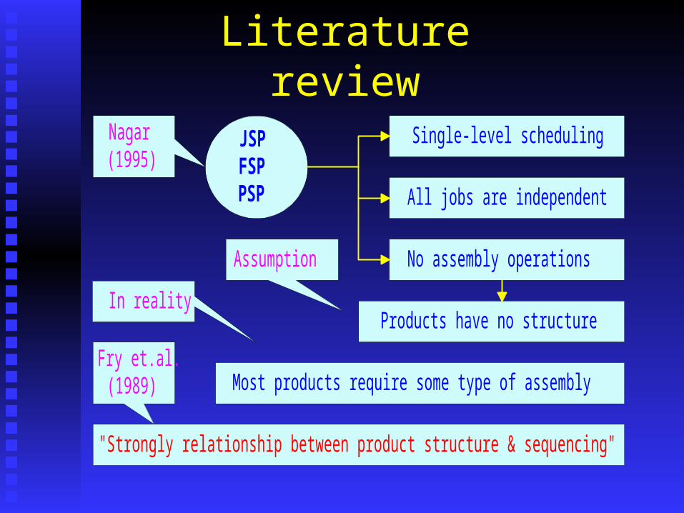
Literature review
JSPFSPPSP All jobs are independent
Single-level scheduling
No assembly operations
Nagar(1995)
Assumption
Products have no structureIn reality
Most products require some type of assembly
"Strongly relationship between product structure & sequencing"
Fry et.al.(1989)
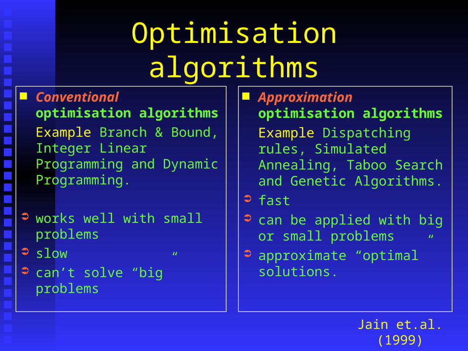
Optimisation algorithms
Conventional optimisation algorithms
Example Branch & Bound, Integer Linear Programming and Dynamic Programming.
works well with small problems
slow can’t solve “big” problems
Approximation optimisation algorithms
Example Dispatching rules, Simulated Annealing, Taboo Search and Genetic Algorithms.
fast can be applied with big or
small problems approximate “optimal”
solutions.
Jain et.al. (1999)
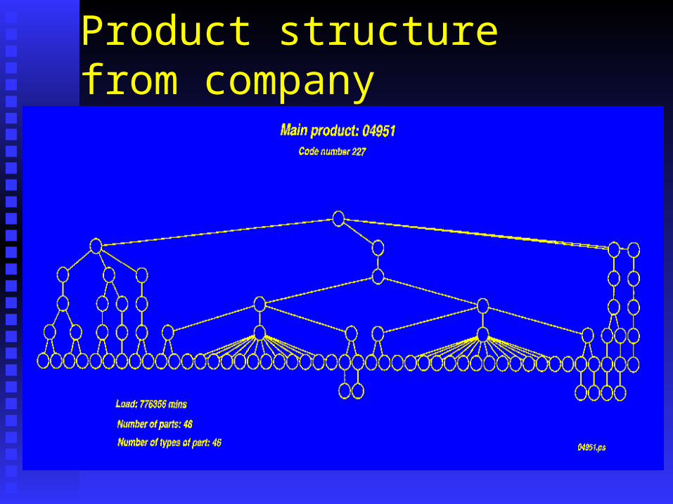
Product structure from company
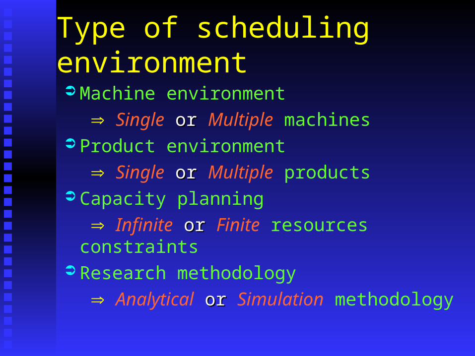
Type of scheduling environment
Machine environment
Single or or Multiple machines Product environment
Single or or Multiple products Capacity planning
Infinite or or Finite resources constraints Research methodology
Analytical or or Simulation methodology
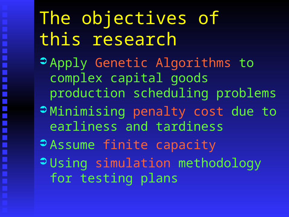
The objectives of this research
Apply Genetic Algorithms to complex capital goods production scheduling problems
Minimising penalty cost due to earliness and tardiness
Assume finite capacity Using simulation methodology for testing
plans
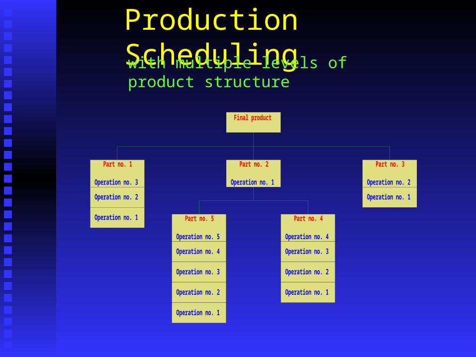
Production Scheduling
Final product
Part no. 1
Operation no. 3
Part no. 3
Operation no. 2
Operation no. 2
Operation no. 1
Operation no. 1
Part no. 2
Operation no. 1
Part no. 5
Operation no. 5
Operation no. 2
Operation no. 1
Operation no. 4
Operation no. 3
Part no. 4
Operation no. 4
Operation no. 2
Operation no. 1
Operation no. 3
with multiple levels of product structure
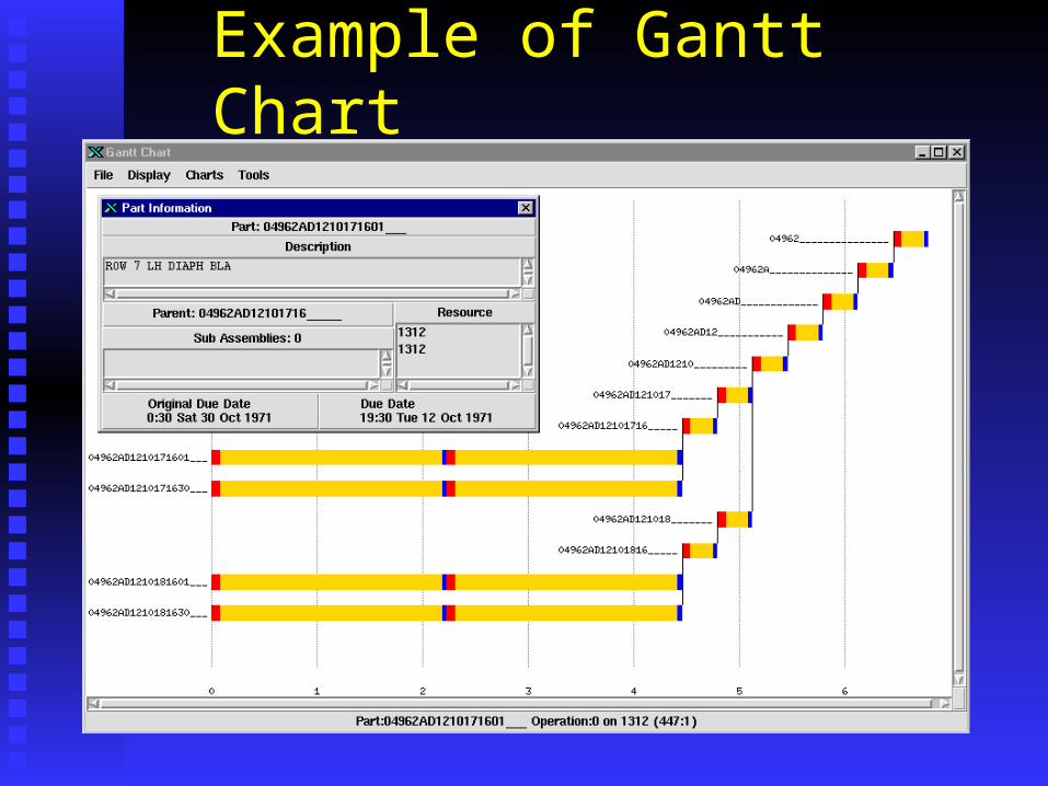
Example of Gantt Chart

Fitness function
Minimise : Pe(Ec+Ep) + Pt(Tp)
Where Ec = max (0, Dc - Fc)
Ep = man (0, Dp - Fp)
Tp = max (0, Fp - Dp)
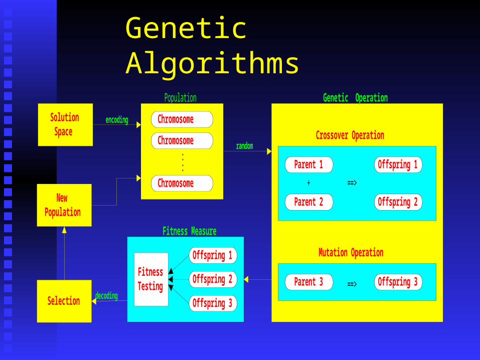
Genetic Algorithms
Chromosome
Chromosome
Chromosome
:: Parent 1
Parent 2
+ ==>
Offspring 1
Offspring 2
Parent 3 ==> Offspring 3
Mutation Operation
Crossover Operation
Genetic OperationPopulation
SolutionSpace
Fitness Measure
Offspring 1
Offspring 2
Offspring 3
FitnessTesting
Selection
NewPopulation
random
encoding
decoding
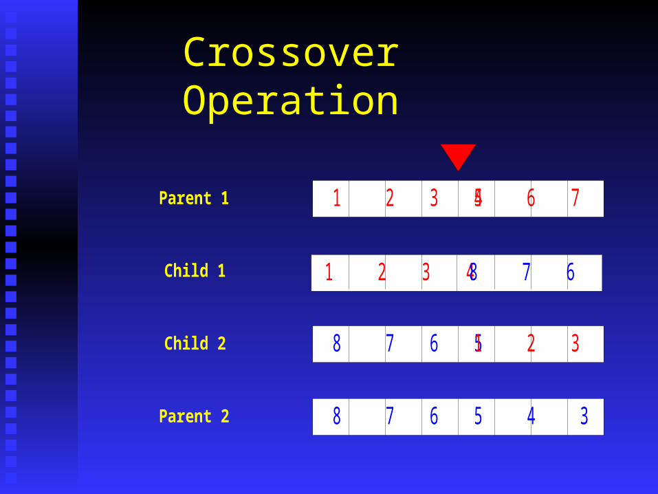
Crossover Operation
1 2 3 4 5 6 7 8
8 7 6 5 4 3 2 1
Parent 1
Parent 2
Child 1
Child 2
1 2 3 4 8 7 6 5
8 7 6 5 1 2 3 4
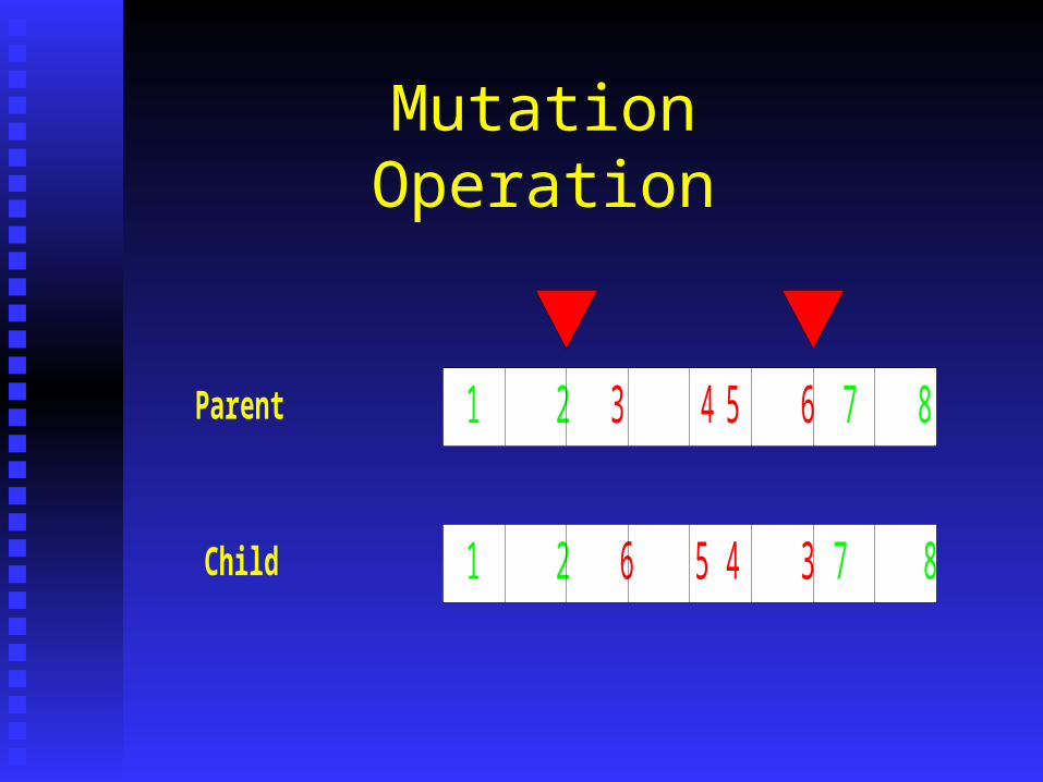
Mutation Operation
1 2 3 4 5 6 7 8Parent
1 2 6 5 4 3 7 8Child
Demonstration of Genetic Algorithm Program
Genetic Algorithms for scheduling problems was written by using Tcl/Tk programming language.
The program was runs on Unix system V release 4.0 on a Sun workstation.
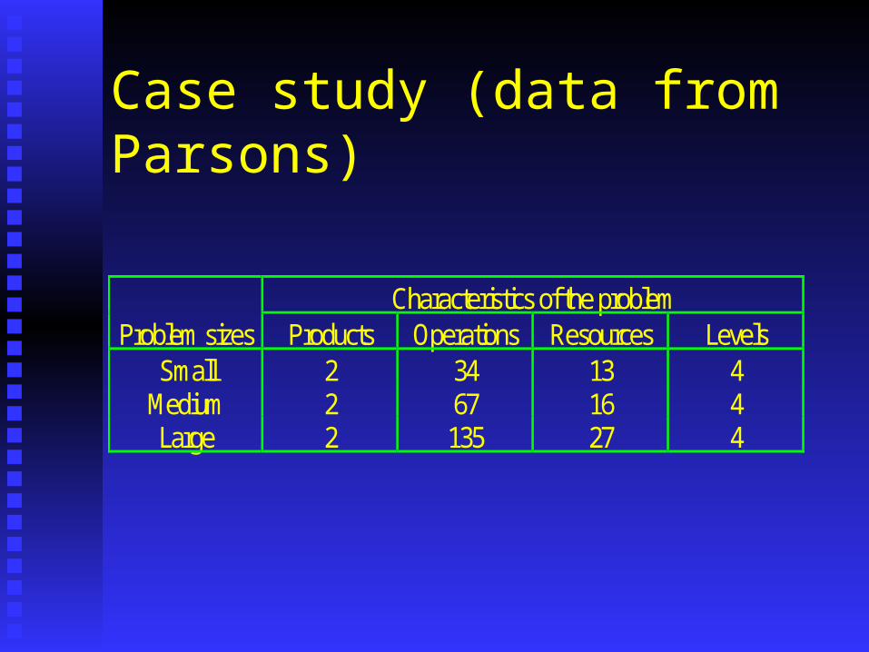
Case study (data from Parsons)
Characteristics of the problemProblem sizes Products Operations Resources Levels
Small 2 34 13 4Medium 2 67 16 4Large 2 135 27 4
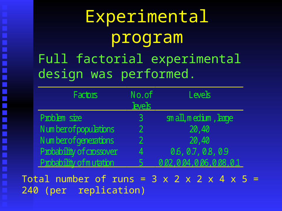
Experimental program
Factors No. oflevels
Levels
Problem size 3 small, medium, largeNumber of populations 2 20, 40Number of generations 2 20, 40Probability of crossover 4 0.6, 0.7, 0.8, 0.9Probability of mutation 5 0.02, 0.04, 0.06, 0.08, 0.1
Full factorial experimental design was performed.
Total number of runs = 3 x 2 x 2 x 4 x 5 = 240 (per replication)
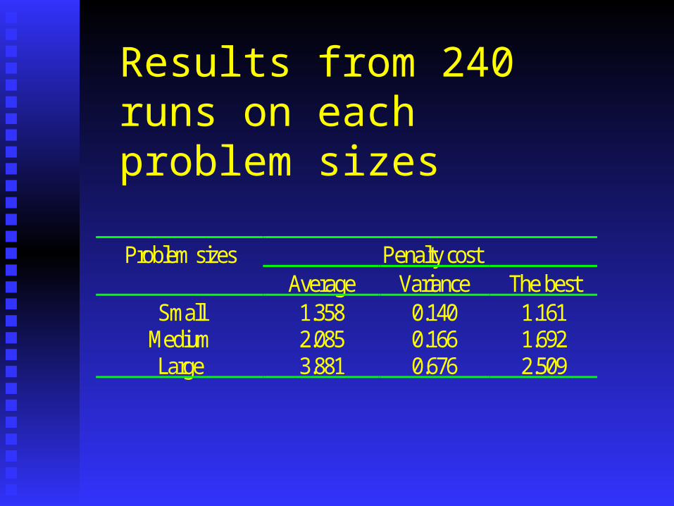
Results from 240 runs on each problem sizes
Problem sizes Penalty costAverage Variance The best
Small 1.358 0.140 1.161Medium 2.085 0.166 1.692Large 3.881 0.676 2.509
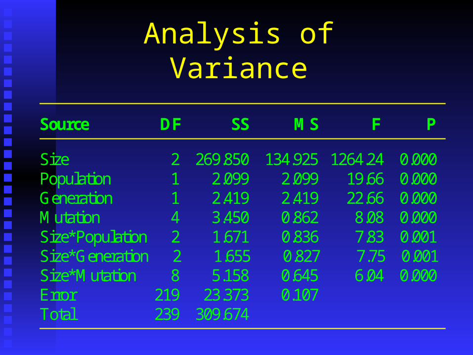
Analysis of Variance
Source DF SS MS F P
Size 2 269.850 134.925 1264.24 0.000Population 1 2.099 2.099 19.66 0.000Generation 1 2.419 2.419 22.66 0.000Mutation 4 3.450 0.862 8.08 0.000Size*Population 2 1.671 0.836 7.83 0.001Size*Generation 2 1.655 0.827 7.75 0.001Size*Mutation 8 5.158 0.645 6.04 0.000Error 219 23.373 0.107Total 239 309.674

The best performance of GAs on the problems
Population average RunningProblem sizes Generation Improve Standard deviation Decreasing Time
first last (%) first last (%) (Min.)Small 2.215 1.242 43.9 0.279 0.033 88.2 2.4
Medium 3.124 1.955 37.4 0.425 0.157 63.1 8.7Large 6.232 2.709 56.5 0.659 0.134 79.7 25.6
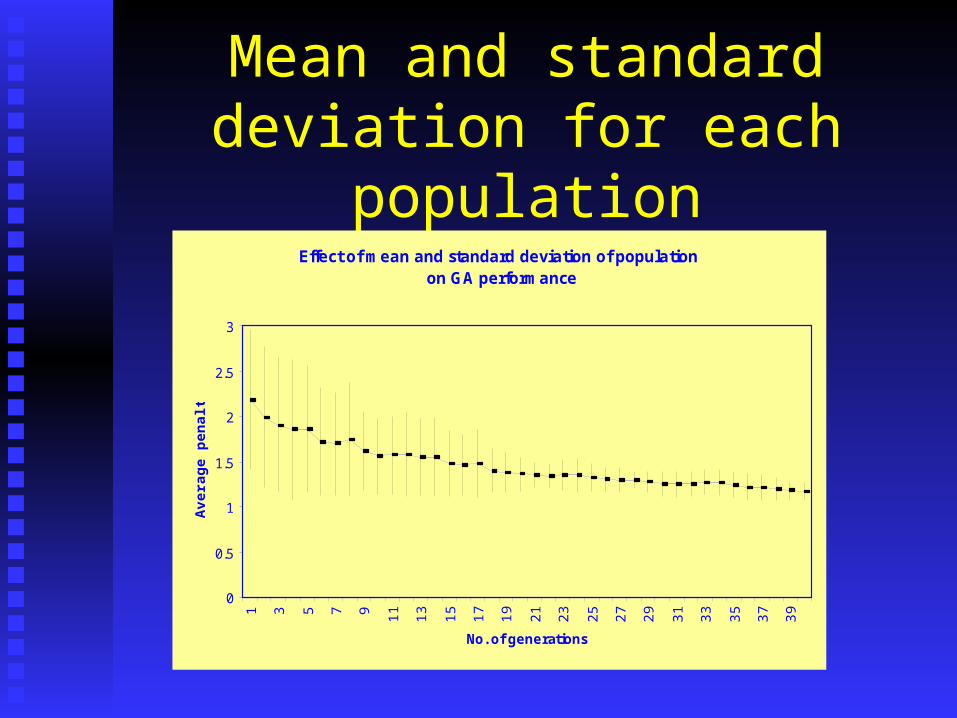
Mean and standard deviation for each population
Effect of mean and standard deviation of population on GA performance
0
0.5
1
1.5
2
2.5
3
1 3 5 7 9 11 13 15 17 19 21 23 25 27 29 31 33 35 37 39
No. of generations
Ave
rag
e p
enal
ty
Discussions
When the problem size increases the execution times increase exponentially.
Next step is to break “large” problems down into smaller independent problems that can be solved in a “reasonable” amount of time.
The solutions to the small problems will be integrated to give an overall solution.
Conclusions
Genetic algorithms represents a powerful technique for solving scheduling problems.
Practical software produced for solving scheduling problems.
Solutions far better than original schedules obtained from Company
Appropriate levels for Genetic Algorithm parameters identified.
Further Research
Bicriteria scheduling problems.
Multiple criteria scheduling problems.

Any questions please ?