Gibbs Sampler in Local Multiple Alignment

Review by 온 정 헌

Topic

하나 . Gibbs Sampler algorithm in Multiple Sequence Alignment( 기전 설명 ) (Lawrence et al., Science 1993; J. Liu et al. JASA, 1995)

둘 . Brief Review of Bayesian missing data problem and Gibbs Sampler ( 개발된 배경… )

Aim of Local MSA

• 기능상 중요한 서열들은 보통 보존되어있다 . (Conserved Sequence)

• Locate relatively short patterns shared by otherwise dissimilar sequences

예 . 1. Regulon 들의 upstream sequence 에 서 Regulatory Motif 찾기 2. Protein 서열의 alignment 를 통해 interaction motif 찾기

Local MSA method• EM(MEME) http://meme.sdsc.edu/meme/website/

• Gibbs sampler (AlignACE, Gibbs motif sampler) http://bayesweb.wadsworth.org/gibbs/gibbs.html

• HMM(HMMER) http://hmmer.wustl.edu/

• MACAW ftp://ncbi.nlm.nih.gov/pub/macaw

Gibbs Sampler AlgorithmIn Practice

(Predictive Update version of Gibbs Sampler)

Problem Description• Given a set of N sequences S1,…,SN

of length nk (k=1,…,N)

• Identify a single pattern of fixed width(W) within each (N)input sequence

• A= {ak} (k=1,…,N) : a set of starting positions for the common pattern within each sequence ; ak=1…nk-W+1

• Objective: to find the “best,” defined as the most probable, common pattern

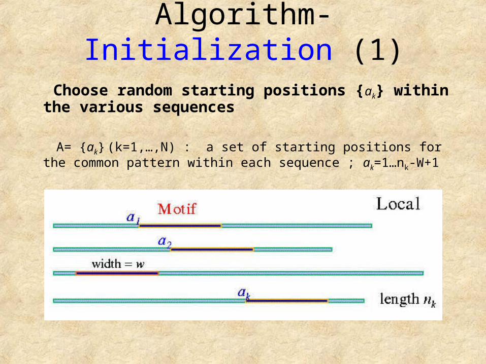
Algorithm- Initialization (1)

Choose random starting positions {ak} within the various sequences

A= {ak} (k=1,…,N) : a set of starting positions for the common pattern within each sequence ; ak=1…nk-W+1

Algorithm- Predictive Update (2)

• One of the N sequences, Z, is chosen either at random or in specified order.

• The pattern description qij and background frequency q0j are then calculated excluding z.

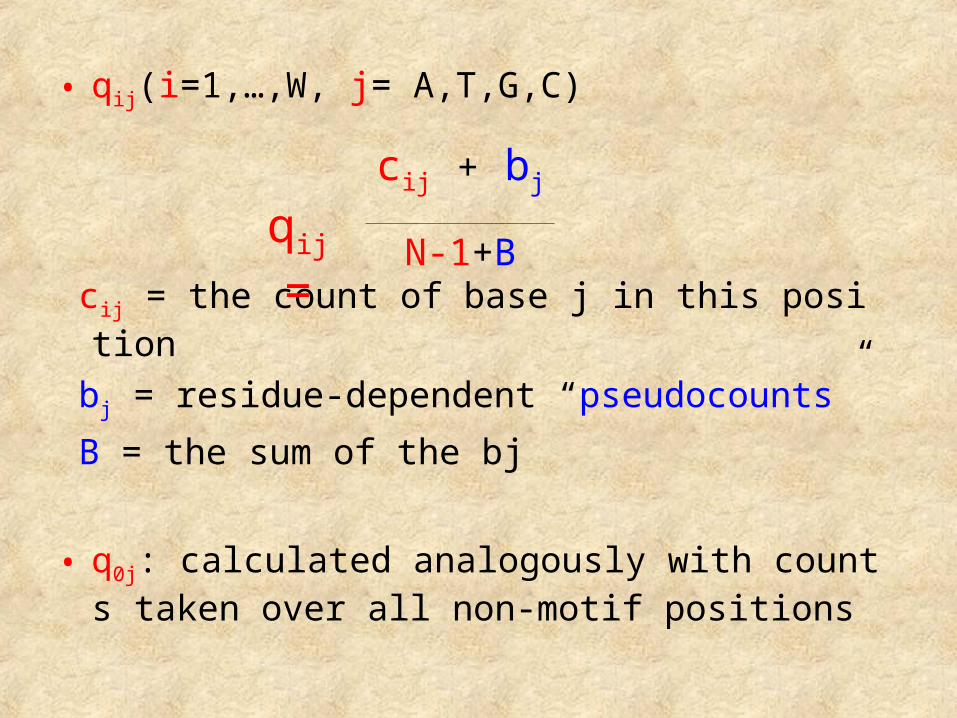
• qij(i=1,…,W, j= A,T,G,C)

cij = the count of base j in this position

bj = residue-dependent “pseudocounts”

B = the sum of the bj

• q0j: calculated analogously with counts taken over all non-motif positions

qij =cij + bj

N-1+B

X X X X X X X X X X X X X Z

X X X X X X M X X X X

X X X X M X X X X X X X

X X X X X X M X X X

X X X X X X X X M X

X X M X X X X X X X

A G G A G C A A G A

A C A T C C A A G T

T C A T G A T A G T

T G T A A T G T C A

A A T G T G G T C A

N=6, W=10

q1A= 3/5, q2G = 2/5, …( 편의상 pseudocount 제외 )

q1G= 0 ( 문제 , pseudocount 꼭 필요 )

Q4*W = q1A q2A …… qWA

q1T q2T ……. qWT

q1G q2G ……. qWG

q1C q2C …… qWC

Q0 4*1 = q0A

q0T

q0G

q0C

A= {a1,a2,…,ak}

Resulting parameters

Algorithm- Sampling step (3)

• Every possible segment of width(W) within sequence z is considered

• The probability Qx (Bx) of generating each segment x according to qij (q0j) are calculated

• The weight Ax = Qx/Bx is assigned to segment x, and with each segment so weighted, a random one is selected.

• Its position then becomes the new az

• Iterations

X X X X X X X X X X X X Z

X X X X X M X X X X

X X M X X X X X X X

X X X X X X M X X X

X X X X X X X X M X

X X M X X X X X X X

A T G G C T A A G C C A T T A A T C G C

q3G X q4G X q5C X q6T X q7A X q8A X q9G X q10C X q11C X

q12A

q0G x q0G x q0C x q0T x q0A x q0A x q0G x q0C x q0C x q0A

AX= Qx/Bx =

Select a set of ak’s that maximizes the product of these ratios, or F

F = Σ 1≤i≤W Σ j∈ {A,T,G,C} ci,jlog(qij/q0j)

Bayesian missing data problem

and Gibbs Sampler

중간 Review

Simulation

• Joint pdf f(x,y,z) 가 주어져있을 때 EX 를 어떻게 구할까 ?

• 원래는 f(x)=∫∫f(x,y,z)dzdy, EX= ∫xf(x)dx

• 그런데 , f(x)=∫∫f(x,y,z)dzdy 를 계산하기 어렵다면 ?…Simulation(sampling)

• x1,x2,x3,….x1000 을 생성시켜 1/m∑xi = EX 으로 approximation

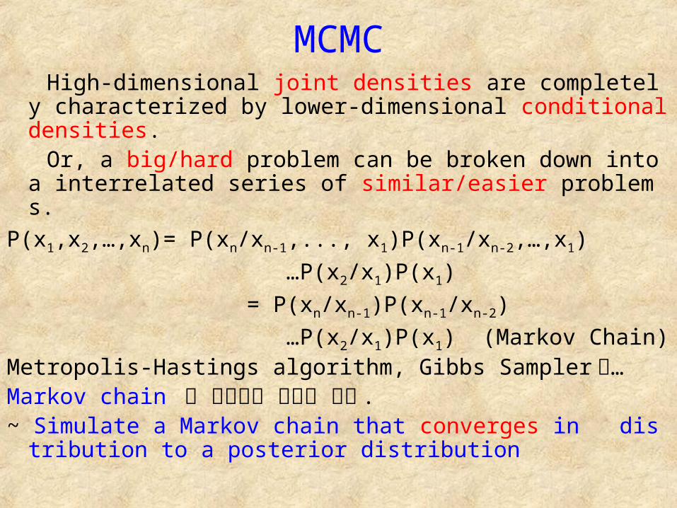
MCMC High-dimensional joint densities are completely charact

erized by lower-dimensional conditional densities. Or, a big/hard problem can be broken down into a inter

related series of similar/easier problems. P(x1,x2,…,xn)= P(xn/xn-1,..., x1)P(xn-1/xn-2,…,x1) …P(x2/x1)P(x1) = P(xn/xn-1)P(xn-1/xn-2) …P(x2/x1)P(x1) (Markov Chain)Metropolis-Hastings algorithm, Gibbs Sampler 등…Markov chain 을 구성하여 문제를 푼다 .~ Simulate a Markov chain that converges in distributio

n to a posterior distribution

Gibbs Sampler(two-component)

(X,Y) 에서 sample 을 하고 싶다면… Choose Y0, t=0;

Generate Xt ~ f(x/yt);

Generate Yt+1~f(y/xt);

t = t+1; iterate

(Y0, X0) (Y1, X1) (Y2, X2),…,(Yk, Xk),…… π (Y, X)~ invariant(stationary) distribution

2-dimension(x1,x2) 의 경우

Gibbs Sampler

Gibbs Sampler

Bayes theorem

Posterior ∝ Likelihood X Prior

잠시 ~~

Bayesian missing data problemΘ: parameter of interestX={x1,…,xN}: a set of complete i.i.d. observations from a density that depends upon θ: π(X┃θ)

π (θ┃X) = Π i=1,…,nπ (xi┃ θ) π (θ) / π (X)

In practical situations, xi may not be completely observed.Assuming the unobserved values are missing completely atrandom, let X=(Y,Z), xi=(yi,zi) i=1,…,n yi: observed part, zi=missing part

π (θ┃Y) = ∫ π (θ┃Y, Z) π (Z┃Y)dZ

Imputation

Multiple values, Z(1) ,…,Z(m) are drawn fromπ (Z┃Y) to form m complete data sets. Withthese imputed data sets and the ergodicitytheorem,

π(θ┃Y) ≈ 1/m*{π(θ┃Y, Z(1))+ … + π(θ┃Y, Z(m))}

But in most applied problems it is impossibleto draw Z from (Z┃Y) directly.

Tanner and Wong’s data augmentation(DA) which applied Gibbs Sampler to draw multiples of θ’s and multiples of Z’s jointly from π(θ, Z┃Y), manages to cope with the problem by evolving a Markov chain.

By iterating between drawing θ from π (θ┃Y,Z) a

nd drawing Z from π (Z┃θ,Y),DA constructs a Markov chain whose equilibrium distribution is π (θ, Z┃Y)

Collapsed Gibbs Sampler(J. Liu)Consider Sampling from π(θ┃D), θ=(θ1,θ2,θ3)• Original Gibbs Sampler

• Collapsed Gibbs Sampler (J. Liu): 계산 용이

Back to Multiple Sequence Alignment

Bayesian missing data problem 과 어떤 관계가… ?

Q4*W = q1A q2A …… qWA

q1T q2T ……. qWT :Parameter of Interest q1G q2G ……. qWG

q1C q2C …… qWC

Q0 4*1 = q0A

q0T

q0G

q0C

A= {a1,a2,…,ak} : Missing Data!B= Given Sequences : Observed Data!

Resulting parameters

Revisiting…

By iterating between drawing Q from π (Q┃A, B) and drawing Z from π (A┃Q, B), DA constructs aMarkov chain whose equilibrium distribution is

π (Q, A┃B)

Collapsed Gibbs Sampler:π (A┃B)

Original Gibbs Sampler algorithm

Step0. choose an arbitrary starting point A0=(a1,0,a2,0,…,aN,0,Q0);

Step2. Generate At+1=(a1,t+1,a2,t+1,…,aN,t+1,Qt+1) as follows:

Generate a1,t+1~π (a1┃ a2,t,…,aN,t , Qt, B);

Generate a2,t+1~π (a2┃ a1,t+1, a3,t …,aN,t , Qt, B);

… Generate aN,t+1~π (aN┃ a1,t+1, a2,t+1 …,aN-1,t+1, Qt, B);

Generate Qt+1~π (aN┃ a1,t+1, a2,t+1 …,aN,t+1, B);

Step3. Set t=t+1, and go to step 1

Collapsed Gibbs SamplerStep0. choose an arbitrary starting point A0=(a1,0,a2,0,…,aN,0);

Step2. Generate At+1=(a1,t+1,a2,t+1,…,aN,t+1 ) as follows:

Generate a1,t+1~ π (a1┃ a2,t,…,aN,t , B);

Generate a2,t+1~ π (a2┃ a1,t+1, a3,t …,aN,t , B);

… Generate aN,t+1~ π (aN┃ a1,t+1, a2,t+1 …,aN-1,t+1, B);

Generate Qt+1 ~ π (Q┃ a1,t+1, a2,t+1 …,aN,t+1, B);

Step3. Set t=t+1, and go to step 1

Predictive Update Version?Predictive distribution

π (A┃B)

A[-k] ={ a1,a2,...,ak-1, ak+1,…, aN}, B: Sequences

π (ak=i ┃A[-k] ,B) …

계산 (Q 에 관한 적분… )…

∝ Л 1≤i≤W(qij/q0j)

<-- why we calculated Ax

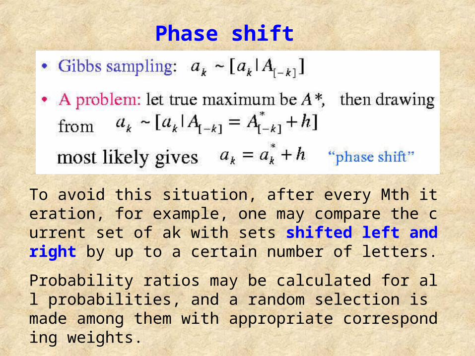
Phase shift

To avoid this situation, after every Mth iteration, for example, one may compare the current set of ak with sets shifted left and right by up to a certain number of letters.

Probability ratios may be calculated for all probabilities, and a random selection is made among them with appropriate corresponding weights.

Convergence 양상

AlignACE 에 포함된 기능-Automatic detection of variable pattern widths

-Multiple motif instances per input sequence

-Both strands are now considered

-Near-optimum sampling method was improved

-Model for base background frequencies was fixed to the background nucleotide frequencies in the

genome being considered

종 합

Lawrence, Liu, Neuwald, Collapsed Gibbs Sampler algorithm in Multiple Sequence Alignment

1993,1994,1995

최근… Gibbs Sampler 를 응용한 motif search program 들 다수 (Gibbs Motif Sampler, AlignACE,)

Dempster, EM algorithm ,1977 Tanner & Wong, Data Augmentation 에 의한 사후

확률 계산 , 1987, JASA (Gibbs Sampler 이용 )