GOMOS VALIDATION REVIEW, DECEMBER 2002

Odile Fanton d’Andon(1)

, Gilbert Barrot (1)

, Jean-Loup Bertaux(2)

, Charles Cot(2)

, Francis Dalaudier(2)

,

Renaud Fraisse (3)

, Didier Fussen(5)

, Marielle Guirlet(1)

, Alain Hauchecorne(2)

, Rob Koopman(6)

, Erkki Kyrölä(4)

,

Antoine Mangin(1)

, Lidia Saavedra(6), Paul Snoeij(6), Viktoria Sofieva(4), Johanna Tamminen(4),

Bertrand Théodore(1), Filip Vanhellemont(5), Tobias Wehr(6)

(1) ACRI-ST,260, route du Pin Montard, Sophia-Antipolis CedexBP 234 F-06904 FRANCE, gomval@acri.fr (2) Service d’Aéronomie du CNRS BP3 - 91371 - Verrieres le Buisson Cedex F- FRANCE, bertaux@aerov.jussieu.fr

(3)Astrium SAS, 31402 TOULOUSE cedex FRANCE, renaud.fraisse@astrium-space.com (4) FMI, P.O.BOX 503, FIN-00101 Helsinki FINLAND, Erkki.Kyrola@fmi.fi

(5) IASB, Avenue Circulaire 3 B-1180 Brussels Belgium , Didier.Fussen@bira-iasb.oma.be (6) ESA

ABSTRACT/RESUME

This paper summarises the status of the GOMOS validation assessed by the GOMOS CAL/VAL team after nine months of the instrument in-flight life. The first GOMOS occultation was successfully measured on March 22, 2002, starting the calibration and verification activity phase. Since this date, more than 50 000 occultations have been performed until the end of 2002. This paper focuses on the status of the GOMOS level 2 algorithms and on the results of the preliminary geophysical validation. Building on the latter, recommendations for algorithms upgrades are provided.

1 GOMOS CAL/VAL

1.1 Overview of the organisation

Within the overall ENVISAT CAL/VAL, coordinated by Guido Levrini, the GOMOS Calibration and Algorithms Verification team has performed his activities according to the tasks defined in the ENVISAT calibration and validation plan [1], [2]. The GOMOS CAL/VAL facilities are located at ACRI-ST (Sophia-Antipolis, France).

The GOMOS CAL/VAL team is composed of engineers and scientists members of ESA, GOMOS ESL (SA, FMI, IASB), ACRI-ST, Astrium, AO CAL/VAL project PIs, SSF as shown in Fig. 1.

Mission planning &

operations

Instrument

performance

Level 1b

verification

Level 2

verification

Level 1&2

validation

P. Snoeij

B. Théodore

A. Hauchecorne

R. Fraisse

O. Fanton d’Andon

R. Fraisse

G. Barrot

J.L. Bertaux

A. Mangin

A. Hauchecorne

O. Fanton d’Andon

R. Koopman

L. Saavedra

G. Barrot

J.L. Bertaux

A. Mangin

A. Hauchecorne

F. Dalaudier

E. Kyrölä

O. Frauenberger

A. Mangin

A.Hauchecorne

F. Dalaudier

O. Fanton

d’Andon

J. Tamminen

V. Sofieva

E. Kyrölä

D. Fussen

C. Cot

F. Vanhellemont

O. Frauenberger

A.Hauchecorne

J. Tamminen

E. Kyrölä

A. Mangin

M. Guirlet

V. Sofieva

O. Fanton

d’Andon

F. Dalaudier

D. Fussen

B. Théodore

R. Koopman

Fig. 1. GOMOS CAL/VAL team (ACRI-ST/Sd’A-CNRS/FMI/IASB/Astrium/ESA)

__________________________________________________________________________________________________________Proc. of Envisat Validation Workshop, Frascati, Italy, 9 – 13 December 2002 (ESA SP-531, August 2003)

A special acknowledgement for useful feedback contributions to the GOMOS products analysis is also given here to Y. Meijer, U. Blum, K.H Fricke, J.B. Renard, , T. Leblanc, S. Migliorini, S. Pal and H. Oelhaf.

The GOMOS CAL/VAL team is in charge of i) the full in-flight calibration and re-characterisation of GOMOS, ii) all the activities required to achieve the complete verification of the level 1b processing models, including: algorithms, auxiliary products, instrument performance and geophysical validation. Within the scope of the commissioning phase activity, the GOMOS CAL/VAL team is also in charge of all the activities required to achieve the verification of the level 2 processing models, including: algorithms, auxiliary products. Lastly, the GOMOS CAL team provides the relevant inputs to the GOMOS mission planning monitoring and to the future routine calibration operations and validation activities.

1.2 GOMOS processing and data distribution

According to [1], an extensive validation program has been established including ground based measurements, ozone sondes, balloons, aircrafts and other satellites. These validating measurements are either results of regular measurements or additional specific measurements for ENVISAT. During the period September-December 2002, 7187 GOMOS occultations were processed and made available at the address: ftp://ftp.fr-acri.com for use by the CAL/VAL team and 26 ENVISAT AO teams. The most intensive work has concentrated on the two selected reference data sets measured during 27-31.7. 2002 and 30.9-3.10. 2002. Both data sets comprise more than 500 occultations in dark limb (Fig.1).

Fig. 1.Geographical distribution of the GOMOS measurements obtained over 4 days, with the local density at a constant pressure level (here, 10 hPa) colour-coded (in units of 1012 mol/cm3). Each point corresponds to one single occultation.

1.3 Objectives

The goal was to achieve by the validation workshop the verification of the processing chain up to L2, as well as to reach a preliminary geophysical validation. Consequently, the objectives of the team activities were:

��To review the Level 2 product algorithms ��To review the geophysical consistency of the GOMOS products ��To provide an error estimation of the Level 2 products ��To recommend instrument re-calibration ��To recommend algorithm upgrades where needed

The status of the instrument performance is thoroughly discussed in [3] together with all the results related to calibration activities. The present paper focuses on the verification of the level 2 algorithms and on the results of the preliminary geophysical validation. It addresses only night side measurements, as it was not possible within the limited time frame of the validation phase to perform an appropriate calibration of the limb signal, thus degrading the quality of results in bright limb. The current characterisation of the limb and straylight contribution to the useful GOMOS signal is addressed in a separate paper [4].

2 STATUS OF THE LEVEL 2 ALGORITHMS

2.1 Brief reminder of the GOMOS mission and processing

Among the three instruments devoted to atmospheric chemistry, the particular role of GOMOS (acronym for Global Ozone Monitoring by Occultation of Stars) is to establish the 3-D distribution of ozone in the stratosphere and to monitor its trend as a function of altitude, thanks to the particularly high absolute accuracy offered by the occultation of stars [5]. The aim of the level 2 processing is to retrieve O3, NO2, NO3, O2, H2O, and in favourable conditions also OClO and BrO, the air density and temperature profiles, the aerosols extinction coefficient and wavelength dependency parameters from the transmission spectra measured by GOMOS as well as information about atmospheric turbulence from the photometers. The principle of the stellar occultation consists in acquiring a star outside the atmosphere (thus providing a reference

stellar spectrum, So(λ)) and tracking it as it sets behind the horizon. The stellar spectrum travelling through the

atmosphere is modified by several phenomena which may be summarised as follows : 1. The refractive effects are the results of the density variation of the atmosphere (versus the altitude) and will modify

the direction and the intensity of any ray as a function of the considered wavelength.

• For a nominal wavelength, the ray will be curved and its curvature increases if the tangent height decreases; this effect is called the geometric refraction. Furthermore, for a given tangent height, the geometric refraction of the ray will increase as the considered wavelength decreases; this latter effect is called the chromatic refraction.

• Without considering losses of energy due to scattering and absorption, we can consider constant the energy flux between two very close rays for a fixed surface. As a consequence of the refraction these two rays will progressively diverge so that the energy effectively received at a given occultation point is diminished. This is the dilution effect.

• Due to turbulence phenomena in the atmosphere, the air density could be considered as a sum of a mean value (say

ρ ) and a fluctuating part (say ′ρ ). Therefore the dilution could be evaluated as the combination of the effect of

what is called the mean dilution (depending on ρ ) and of the scintillation (linked to ′ρ ). The limit between these

two aspects depends on the perturbation length scale affecting the density. Depending on the retrieval method, the scintillation could be considered as a noise affecting the final spectrum or could be considered as an additional source of information.

• The variation of the dilution as a function of wavelength can be modelled accurately; this correction takes into account the amplitude variation (with wavelength) of the scintillation. This is called the chromatic dilution.

2. The scattering and the absorption effects, although of different nature, are gathered under the same convenient

terminology extinction.

The spectrum S(λ,z) is modified by the absorption of all atmospheric constituents integrated over the line of sight from GOMOS to the star, according to the Beer-Lambert law :

[ ]0( )

( , ) ( ) exp , ( ) ( )i i

i

S z S T l n l dlσ λΓ

� �λ = λ −� �� ��� (1)

where λ is the wavelength, z is the tangent altitude of the line of sight, ni(l) (mol./cm3) is the molecular density and σι the cross section of species i which depend on the temperature. Actually, this dependence σ σ

i iT)= ( is not very

strong for most of the atmospheric components; so, the inversion process is initialised considering that σi depends

only on the wavelength, the temperature is considered uniform and equal to the one at the tangent point. Under this assumption, the formula (1) may be simplified as follows:

[ ]0( , ) ( ) exp , ( ) ( )

i i

i

S z S T z N zσ λ� �λ = λ −� �� �� (2)

introducing the integrated density Ni(z) (mol./cm2) of the species i along the line of sight (referred to as the “slant

column density”).

When the occulted spectra are divided by the reference spectrum, measured out of atmosphere, nearly calibration-free horizontal transmission spectra are obtained, assuming the instrument response function does not change during one occultation; lasting typically 30 to 40 seconds. These transmissions provide the basis for retrieval of atmospheric constituents density profiles, which benefits from the fact that observing the star light confines the measurement to a "thin" well-defined volume. The transmission including the conjugated effects of the absorption and the dilution - assumed to be decoupled – is indeed approximated as :

.

sd aT T T= (3)

The refractive part, Tsd, consists of the refractive dilution part and the modulation part caused by the scintillations. In the GOMOS processing, an external model (ECMWF for altitude below 50 km combined with MSIS-90 model above) provides estimation for the dilution part and photometers are used to estimate the modulations by scintillations. The extinction part, Ta, is the basis for geophysical retrieval of constituent densities: the retrieval technique applied by the GOMOS Level 2 processing splits the inversion problem into a spectral inversion and a vertical inversion using the effective cross section method and making an approximation for the integration time averaging. The spectral inversion produces slant column densities for different constituents by fitting a modelled extinction transmission to the observed transmission corrected for refraction effect [6]. All constituents are retrieved simultaneously and all wavelengths excluding the O2 bands (i.e. [200,627.7] + [630.3,686.7] nm) are used. The vertical density profiles are the result of the vertical inversion of slant column densities, with the assumption of linear variation between two measurement points. Spectral and vertical dependences of aerosol extinction are also estimated from transmission data. Lastly, from the analysis of fast photometers signals, high resolution temperature and density profiles are calculated.

2.2 Level 2 processing chain verification (step by step)

In line with [1], the basic step by step verification of the level 2 algorithms has been performed before the CAL review meeting, working on specific occultation, especially R00799/S081 which had the advantage to be coincident with a lidar measurement. Two tasks were performed in parallel :

1) Thorough detailed step by step analysis to check the complete correctness of the processing and to optimise the tuning of the level 2 configuration parameters

2) Global and statistical analysis of the reference data set to try to sort out the pathological cases and classify them as a function of latitude and altitude ranges.

The internal correctness of each individual processing step has been successfully checked and the derivation of the associated error budget has been attempted although not yet completed at the end of 2002. GOMOS is a special case: the error not only depends on the measured quantity but also on the star magnitude and spectrum shape (colour, or temperature of the star). In addition, the scintillation effect which distorts somewhat the shape of the stellar spectrum makes the disentangling analysis of the various contributors to the error budget more complicated.

1) Scintillation/dilution correction : the complete algorithm has been checked against breadboard by A. Hauchecorne (SA) with the conclusion that it behaves as expected. Unfortunately, the algorithm cannot account for the effect of the isotropic turbulence which seems to be a strong contributor to the overall noise budget that would explain the bad retrieval results observed in a number of cases (see spectral inversion below).

2) Spectral inversion : A particular emphasis was (and is still to be) given to the spectral inversion extracting the slant column densities Ni from the atmospheric transmission Ta for the reason that it is the heart of the GOMOS retrieval. It is a strongly over-determined problem (hundreds of spectral pixels measurements yielding a few unknowns Ni ), and also the retrieval is affected by the particular spectrum and intensity of the star, and various atmospheric effects (absorption, refraction, scintillation) distort the transmission spectrum and must be taken into account in the retrieval. In addition, the absorption is a non-linear function of slant column densities, calling for non-linear least square fit algorithms. An analysis, performed by A. Hauchecorne (SA), focused on residual extinction spectra, using the different reference data sets and computing their variance (Fig. 2). If the transmission model is perfect, Vcor should be around 0. This is verified at high altitude.

80x103

60

40

20

Altitude m

10-7

10-6

10-5

10-4

10-3

Variance corrected from noise

The variance V of the residual spectrum Res=Tcor-Tmod is computed for each spectrum between pixels 454 and 1396. Tcor : transmission corrected for scintillation-dilution Tmod : Model transmission In order to suppress the contribution of measurement noise (assumed white noise), a 5 points running mean is applied to the residual spectrum and the variance Vsmo of the smoothed spectrum is computed.

The corrected variance is taken equal to : Vcor =Vsmo-V

Fig. 2 : Variance corrected for photon noise in RDS V3 for the 4 brightest stars (stars 1, 2, 8, 9). Spectra with uncorrected variance greater than 3.10-4 have been suppressed (this represents about 5% of spectra).

Residual spectra present a systematic deviation from 0 below 42 km, with a maximum of 1% (10-4 in variance) around 32 km. This value is reduced to 0.7% (5.10-5 in variance) when the spectral range is reduced to 512-627 nm. The altitude of the maximum corresponds approximately to the expected altitude for the transition from weak turbulence above to strong turbulence below. We have to keep in mind that the residual variance also includes all terms that are not accounted for in the transmission model. For instance, if the presence of scintillations degrades the spectral inversion with the present algorithm, as it seems to be the case for NO2 and NO3, this will contribute to the estimated variance. The characteristics of the autocorrelation functions which have been computed are consistent with the hypothesis that spectra are perturbed by small scale refractive structures. However, they do not seem to fit perfectly with the hypothesis of pure isotropic turbulence. There is probably a mixing between isotropic and anisotropic (stratified) perturbations to be further investigated in the future.

3) Error on Tmod & loop over cross-sections : Currently, the error on Tmod is set to zero which is a too poor approximation in some cases. Furthermore, for the sake of simplicity in the current still on-going investigation phase, there is currently no iteration over temperature of cross-sections.

4) Smoothing : the initial nominal method was a smoothing with an adaptive cubic spline, which made the level of smoothing variable with the data. As a consequence, the vertical resolution after smoothing was not known. An alternative method has been implemented in the course of the commissioning : a Gaussian filter with the advantages that i) the level of smoothing is under control, ii) the error bar is decreased by 2 compared to un-smoothed profiles, iii) the anti-correlation between layers is almost suppressed. A minimum smoothing parameter was applied so far as the objective was to look at as raw data as possible during this phase in order to more easily point out toward any unexpected discrepancy and also to assess the true accuracy and vertical resolution of the GOMOS retrieved profiles.

The outcomes of the validation (see, e.g. Fig. 3) have clearly demonstrated the need to revise the vertical sampling below 20 km (currently of the order of 600 m due to refraction effects).

5) Vertical inversion : checked and proven to work correctly. The only problem was related to the writing in the level 2 product where negative values were set to a minimum value. This problem is corrected in the latest implementation of the processing chain.

6) Aerosols : some tests were performed at ACRI by Didier Fussen (IASB) in favour of a degree one polynom against a law in 1/lambda. All the reference data set are thus retrieved with a polynom of degree one since then. Taking into account the other issues, there is still, of course, a need of consolidation rendered difficult by the current low level of stratospheric aerosols.

7) H2O,O2 : the algorithms have been preliminary checked by Jean-Loup Bertaux (SA). Transmission spectra are compared with HITRAN line-by-line calculations of the model transmission Tmod. Concerning H2O, a refined analysis should be performed, in order to find an accurate wavelength assignment: a simple constant shift along the whole spectrum might not be sufficient to get a perfect match over the whole wavelength range. Also, a refined study of the actual measurement spectra should be pursued, in order to identify persistent differences between measured and model transmission, with a possible revision of the HITRAN data base, or the identification of additional lines or absorbing species. Concerning O2, the external validations which were performed by comparing the GOMOS O2 retrievals with ECMWF data show an important bias, with more O2 in the GOMOS retrieval than predicted by ECMWF. The bias factor is of the order of 1.5; it will be important, in the near future, to determine if this bias factor is constant or not. If it is reasonably constant, then a short term solution would be to include the bias factor in the retrieval. Of course, it would be also recommended to understand the cause of this bias in the retrieval; comparisons with solar occultation transmissions measured by ILAS on ADEOS, or measured in balloon borne instrument during CAL-VAL activities of ENVISAT should be instructive in this respect.

To summarise, the main lessons from these GOMOS ESL team studies are illustrated on Fig. 3 which displays typical GOMOS ozone profiles relative difference with external sources in dark limb conditions. Three regimes appear which points towards the main characteristics of the current GOMOS retrieval : 1. excellent above 40 km, 2. fluctuations of the order of +/- 20% due to scintillation effects in the altitude range 20-40 km, 3. high fluctuations below 20 km, due to a combined effect of weak SNR and the current vertical sampling (only minimal smoothing is applied).

Fig. 3 : Main characteristics of the current GOMOS ozone retrieval : 1. excellent above 40 km, 2. fluctuations of the order of +/- 20% due to scintillation effects, 3. high fluctuations below 20 km due to a combined effect of weak SNR

and the current vertical sampling (only minimal smoothing is applied).

3 GOMOS PRODUCTS ASSESSMENT

Preliminary evaluation of the geophysical content of GOMOS products has been performed by comparing them with climatology and external sources. This section addresses the activities specifically carried out by the GOMOS CAL/VAL team. Much more work was performed in the frame of the ENVISAT validation by other ACVT teams; among others, the reader is in particular referred to [7], [8], and [9]. The summary section (§3.5) integrates the conclusions provided either by internal investigation or from external sources.

3.1 GOMOS level 2 product overview

Level 2 products are geophysical data. Their main characteristics are listed below

Turbulence MDS (sampling rate 40 Hz – below 50 km – dark limb only)

• High resolution temperature profile (HRTP)

• Product Confidence Data (PCD) including error estimates of Temperature

• Air density profile

• Tangent altitude

Tangent line densities MDS (sampling rate 2 Hz – below 120 km)

• Tangent line density profile for Air, O3, NO2, NO3, OCLO, O2 and H2O

• Associated standard deviations and PCD

Aerosols MDS (sampling rate 2 Hz – below 120 km)

• Aerosol tangent integrated extinction profile + standard deviation + spectral parameters and PCD

• Aerosol extinction coefficient profile + standard deviation + spectral parameters and PCD

Local density MDS (sampling rate 2 Hz – below 120 km)

• Local density profile for Air, O3, NO2, NO3, O2, H2O, OCLO

• Associated standard deviations and PCD

Geolocation ADS

• Geometry of the occultation

• Temperature and pressure profiles from external model

• Re-built air density and temperature profiles (combining internal and external contributions)

Accuracy estimation ADS

• Covariance matrix after spectral and vertical inversion where MDS means Measurement Data Set and ADS means Auxiliary Data Set.

3.2 GOMOS turbulence MDS (HRTP) assessment

3.2.1 Introduction

This section presents the comparison of the high-resolution air density and temperature profiles distributed in the Level 2 product files in the measurement dataset NL _Turbulence with reference air density (ECMWF). This work was performed by the FMI team (V.Sofieva E.Kyrölä, J.Tamminen). The reference dataset version 2 of July 2002 (noted RDS2) is analysed. For comparison purposes, the error of temperature reconstruction is transformed to absolute values.

3.2.2 Uncertainty of ECMWF data

It is known that the ECMWF data have high accuracy in lower atmosphere: its uncertainty can be approximated by a linear function, increasing from 2% to 18% in the range 0 -120 km, e.g. [10]. Uncertainty of ECMWF temperature profile is 1-2 K for altitudes 0 -30 km, for altitudes 30-60 km it grows almost linearly from 2 K to 15 K and for upper atmosphere the temperature uncertainty is 15 - 20 K that corresponds to climatology [11].

3.2.3 Product overview

The vertical resolution of high-resolution products is better than 200m and it covers the altitude range 15-40 km. Fig. 4 presents the distribution of minimal and maximal altitude in the reference dataset 2 (July). As it follows from the figure,

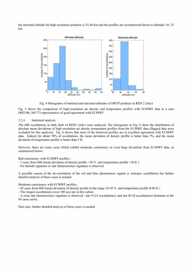
the maximal altitude for high resolution products is 35-40 km and the profiles are reconstructed down to altitudes 10- 25 km.

Fig. 4 Histograms of minimal and maximal altitudes of HRTP products in RDS 2 (July)

Fig. 5 shows the comparison of high-resolution air density and temperature profiles with ECMWF data in a case (R02186_S0177) representative of good agreement with ECMWF.

3.2.4 Statistical analysis

The 600 occultations in dark limb of RDS2 (July) were analysed. The histograms in Fig. 6 show the distribution of absolute mean deviations of high resolution air density temperature profiles from the ECMWF data (flagged data were excluded for this analysis). Fig. 6 shows that most of the retrieved profiles are in excellent agreement with ECMWF data. Indeed, for about 70% of occultations, the mean deviation of density profile is better than 5%, and the mean deviation of temperature profile is better than 5 K.

However, there are some cases which exhibit moderate consistency or even large deviations from ECMWF data, as summarised below.

Bad consistency with ECMWF profiles : - 7 cases from 600 (mean deviation of density profile >30 % and temperature profile >30 K ) - No latitude signature or star characteristics signature is observed. A possible reason of the de-correlation of the red and blue photometers signals is isotropic scintillation but further detailed analysis of these cases is needed. Moderate consistency with ECMWF profiles : - 49 cases from 600 (mean deviation of density profile in the range 10-30 % and temperature profile 8-40 K ) - The longest occultations (over 200 sec) are in this subset. - A clear star characteristics signature is observed : star 9 (14 occultations), and star 84 (8 occultations) dominate in the 49 cases series. Here also, further detailed analysis of these cases is needed.

Fig. 5 Comparison of high-resolution air density and temperature profiles with ECMWF data: occultation R02186_S0177. Left top : air density profiles. Left bottom : temperature profile. Red line presents reconstructed high-

resolution profile; pink lines present 1-sigma error bars. Right top: relative deviation of density profile from the ECMWF data in percent. Right bottom: absolute deviation of temperature profile from ECMWF data

Fig. 6. Distribution of mean deviations from ECMWF density and temperature profiles

3.2.5 PCD values in NL_TURBULENCE

The PCD values represent 10 times the relative errors of retrieved temperature in percent. For flagged values PCD=65000. Fig. 7 shows the histogram of percentage of flagged data in RDS2 (July). For other data, the estimated error seems to be overestimated. Fig. 8 presents the histogram of the estimated error for the occultation R02186_S0177, beyond the deviation derived from ECMWF data (3.6 K for temperature). It can be observed that the estimated error significantly exceeds the deviation from the ECMWF profile and the uncertainty of the ECMWF data.

Fig. 7. Percentage of flagged data in RDS2 Fig. 8. The histogram of the estimated errors of

temperature for occultation R02186_S0177. Flagged values are not included

3.3 GOMOS Air density in Local density MDS assessment

3.3.1 Introduction

This section presents the comparison of the air density profiles distributed in the Level 2 product files in the measurement dataset NL_LOCAL_SPECIES_DENSITY with reference air density (ECMWF). This work was performed by the FMI team (V.Sofieva, E.Kyrölä, J.Tamminen). The same reference dataset version 2 of July 2002 (noted RDS2) as in the previous section is analysed.

3.3.2 Product overview

Fig. 9 shows comparison of the reconstructed air density and temperature profiles with ECMWF data. Note that more examples can be found in supporting movies. In many cases, the reconstructed Level 2 air density profile significantly fluctuates around the reference profile.

Fig. 9 Comparison of Level2 air density with ECMWF data : bright star (star 9). Left : Level 2 air density profile with error bars (1-sigma), ECMWF profile. Right: relative deviation of density profile from the ECMWF data in %

3.3.3 Statistical analysis

The 600 occultations in dark limb of RDS2 were analysed. The main attention was given to the following questions:

• Is the distribution of the deviations from ECMWF profile unbiased? The unbiased distribution indicates that the fluctuating behaviour of reconstructed profiles can be explained by the noise in the measurements, which is expected to be Gaussian or approximately Gaussian.

• What is the range of deviations from the reference profile?

• What is the altitude dependence of the deviations

Fig. 10 shows the relative deviations from ECMWF air density profile in the reference dataset. 'The cloud' of deviation extends beyond the 100%-level. The green line corresponds to mean of this distribution and the blue line shows the median. For the altitudes 20 - 50 km the mean and median are almost coincidental, while for upper stratosphere these lines significantly deviate from each other. Similarity of mean and median indicates that the distribution is symmetric: estimation of the quantity of interest (here: air density) is unbiased. For altitudes above 50 km as well as ~15 km, the mean and the median differ. It indicates that the distribution contains outliers. Let us also note that the median (more robust characteristic of the 'center' of distribution in presence of outliers) is around the zero-line. Therefore, we can conclude that the median of the reconstructed air density is in good agreement with ECMWF data.

Fig. 11 shows the histograms of the deviations from the ECMWF profile that are plotted for 2 km thick layers and presented as a shaded contour plot. The histograms are normalized by the number of points, so that Figure 4 presents

the estimated probability density function for each altitude. For all altitudes it is Gaussian-like with the standard deviation of ~ 10% for the altitude range 15- 35 km, which slightly exceeds the estimated error plus uncertainty of ECMWF data .

Fig. 10. Deviations from ECMWF density profiles in reference dataset 2 (July).

Fig. 11. Histograms of deviations vs altitude

Fig. 12 presents the percentiles of deviations from ECMWF data in the reference dataset.

Central red line is the median; 25 % lines bound the region containing 50% of all data; 10% lines - the 80%-interval (10% of point from each side is outside this range). This figure shows:

1) 50 % of data have deviation from ECMWF profiles less that 20% in the altitude range 15- 40 km. 2) The shape of the percentiles curves is similar to the error estimation curves.

Fig. 12. Percentiles of deviations from ECMWF profiles

3.4 GOMOS ozone density in Local density MDS assessment

3.4.1 Introduction

This section presents the comparison of the ozone density profiles distributed in the Level 2 product files in the measurement dataset NL_LOCAL_SPECIES_DENSITY mostly with zonal and monthly average profiles from Fortuin and Kelder (F-K) climatology (1998) [12]. This work was performed by the M. Guirlet (ACRI-ST).

3.4.2 Product overview

As first examples, Fig. 13 shows the comparison of two individual profiles (one in September, the other in July) with corresponding latitudinal climatology profile and Fig. 14 shows the comparison with a GOMOS O3 profiles zonal average. We note that the agreement is excellent.

Fig. 13: left: comparison between R03057/S009 (30/09/02, 25.9°N, 101.3°E, black solid line) and F-K climatological profile and variability profile (September, 30°N, orange line); right: comparison between R02129/S135 (27/07/02,

0.24°N, 39.89°E, black solid line) and F-K climatological profile and variability profile (July, 0°N).

Fig. 14. Average O3 profile for GOMOS measurements in 10N-20N for the period 28/07/02 – 31/07/02 compared with the vertical profile of the F-K climatology; the dispersion bar attached to the GOMOS results is the 1 sigma dispersion

of all the GOMOS measurements in this range of latitude and altitude and for this period.

3.4.3 Statistical analysis

Several thousands of occultations were analysed, including the two reference data sets. The main attention was given to the following questions :

• What is the consistency with climatological profiles ?

• Is there latitude or star characteristics signature ?

• Do we observe deficiencies of processing ? Comparisons on two limited periods (dataset for orbits between 2129 and 2187, dates between 27/07/02 and 31/07/02, and dataset for orbits between 3056 to 3103, dates between 30/09/02 and 03/10/02) allowed to identify profiles showing oscillations in the vertical scale which exceed atmospheric variability. This anomaly generally occurs for the same star during successive orbits. It is more frequent at high latitudes (northward of 60°N and southward of 60°S), but also happens at mid and low latitudes. It is most of the time associated with strong oscillations of the air density vertical profile, indicating a deficiency of the inversion algorithm as the most likely cause for this anomaly. Detailed investigation clearly demonstrated that the origin of these oscillations is a too strong background signal. For a few of them (S038 and S052), the occultation is considered as a dark limb occultation whereas it occurred at least partly in bright limb conditions.

The relative difference (GOMOS-climato) was calculated for a longer period (orbits between 1204 and 3805, dates between 24/05/2002 and 21/10/2002) at different pressure levels and within different latitude bands. The variability of this difference is larger at high latitudes (both hemispheres). Fig. 15 shows the results obtained in the latitude band [-5°,+5°].

Fig. 15. Individual GOMOS measurements at equator and at various pressure levels are plotted according to day of the year, with the ordinates displaying the relative difference with the reference O3 mixing ratio of the Fortuin-Kelder

climatology. At the two highest levels of 1 and 0.3 hPa, GOMOS is higher than climatology most likely due to GOMOS night side measurements ,while the climatology reflects also day side measurements.

This kind of systematic study allowed us to check the reasonable agreement for some O3 profiles (in terms of altitude and amplitude of the O3 maximum for instance), and to identify occultations with strong anomalies, mostly related to background contribution.

3.4.4 Comparison with external sources

The validation results obtained by comparison with lidars deployed in the NDSC are extensively discussed in [7]. However, it is worth mentioning in this section a comparison performed at ACRI-ST comparing two coincident GOMOS measurements with the Mauna Loa lidar (courtesy of T. Leblanc, S. Mc Dermid, JPL; P. Keckhut, IPSL/CNRS). Fig. 16 shows the relative difference of vertical ozone profiles from two occultations : R02967/S009 and R02967/S143 on the same orbit with the lidar measurement. Fig. 17 displays the corresponding three ozone profiles. We note the very good agreement with the lidar profile as well as the excellent consistency of the two GOMOS profiles.

Fig. 16. Relative difference of vertical ozone profiles from two occultations : R02967/S009 and R02967/S143 with the Mauna Loa lidar measurement

Fig. 17. Vertical ozone profiles from two occultations : R02967/S009 (blue) and R02967/S143 (green)

with the Mauna Loa lidar measurement (+ 1 σ standard deviation)

GOMOS profiles were also successfully compared with POAM and Haloe data. For the latter, 1717 O3 profiles

between 30/05/02 and 07/10/02 were compared (acknowledgements: J.M. Russell III and the Langley Research Center,

E. Thompson (NASA), L. Deaver (NASA), ETHER (CNES/IPSL)). Statistical results are displayed on Fig. 18 and show a good agreement in the altitude range : 20 – 50 km.

Fig. 18 : Mean and median profiles of the relative difference between GOMOS and Haloe over 1717 profiles.

3.5 GOMOS level 2 product status summary

General lessons on the observations

• Large difference between observations in dark or bright limb

• Degraded results in twilight conditions

• Large oscillations at the bottom of the profiles

• Error estimates underestimated with one exception for HRTP product. Ozone product :

• Individual differences up to 20 %

• Excellent mean profiles : no bias with lidar and bias less than 10% with other sources

Air product :

• The reconstructed Level2 air profile significantly fluctuates around the reference profile

• Median of deviations from ECMWF profile is unbiased. However, small bias (up to 5%) around 25 km altitude is observed.

• 50 % of data deviate from the ECMWF profiles by less than 20 % in the altitude range 15-40 km. It points to overall consistency with the ECMWF data.

Temperature product (low resolution) :

The low resolution product is derived from a combination of GOMOS data and model – ECMWF/MSIS.

• Criticism. Lack of knowledge about model contribution.

Temperature product (high resolution profile - HRTP)

• very promising (agreement with ECMWF better than 5K in 70% of cases)

• The estimated error of temperature reconstruction contains 20 to 40% of flagged data. For non-flagged data the error is overestimated. The revision of the error estimation is recommended.

NO2 and NO3 products : • Retrieval may be improved by changes in the algorithm (DOAS like method).

H2O product :

• very preliminary;

• realistic in UTLS since last spectral re-calibration (end of November – V4)

O2 product :

• show bias

• need scientific study of algorithm and/or � database

4 CONCLUSIONS-RECOMMENDATIONS

The GOMOS level 2 processor has been proven to be healthy and robust enough to process the entire GOMOS data without trouble. Although the products are in general promising the validation team recommends a number of actions that are listed below with a tentative time table:

Level 2 - Algorithms :

Short term – emergency (test and specifications within 6 months) 1.Experiment and qualify alternative spectral inversion schemes (in relation with scintillation effects) 2.Qualify and adapt smoothing in vertical inversion 3.Improve the error estimates and quality indicators (to be continued) Medium term (within 12-18 months) 1.Specify modelling error 2.Experiment and qualify the full covariance matrix method 3.Compute averaging kernels and provide them in products 4.Investigate the use of SFA (Steering Front Assembly) angles to derive refraction angle and density profiles 5.Improve the O2/H2O retrieval scheme and solve present weaknesses Long term 1. Experiment coupling of spectrometers 2.Other species retrieval (OClO, …) 3. Study aerosol model variations and the use of a priori information

Level 2 – algorithm tuning :

Short term (2003) 1. Tuning of High resolution Temperature Profile processing parameters and its error estimates 2. Check temperature effects in spectral inversion (p-loop)

Level 2 – products updates :

Short term (2003) 1.New temperature/density products : GOMOS only (Rayleigh + O2 + HRTP) and external ECMWF+MSIS profiles 2.Add HRTP product into the meteo product 3.Solar zenith angle at tangent point should be provided

5 REFERENCES

1. ENVISAT Calibration and Validation Plan, PO-PL-ESA-GS-1092. 2. GOMOS Calibration-Validation Plan, ref. PO-AD-ACR-GS-0003 3. Barrot G., et al. GOMOS Calibration on ENVISAT – status at end of December 2002, ENVISAT validation workshop proceedings, 2002 4. Mangin A., et al. Limb and straylight contribution to GOMOS signal – status at end of December 2002, ENVISAT validation workshop proceedings, 2002 5. Bertaux, J-L., et al. Monitoring of ozone trend by stellar occultations: The GOMOS instrument, Adv. Space Res., 11(3):237-242, 1991. 6. Kyrölä, E., et al. Inverse Theory for Occultation Measurements 1. Spectral Inversion, J. Geophys. Res., 98, 7367-7381, 1993.

7. Keckhut P., et al. Validation of GOMOS ozone profiles using NDSC lidar : statistical comparisons, ENVISAT validation workshop proceedings, 2002 8. Marchand S., et al. Validation of GOMOS air density and temperature profiles, ENVISAT validation workshop proceedings, 2002 9. Renard J.P. et al. Validation of GOMOS products using SALOMON algorithms and data, ENVISAT validation workshop proceedings, 2002 10. Palmer P.I et al: A nonlinear optimal estimation inverse method for radio occultation measurements of temperature, humidity, and surface pressure. Journal of Geophysical Research, Vol. 105, No. D13, pp. 17513-17526, 2000. 11. Rieder M. and G. Kirchengast: Error analysis and characterization of atmospheric profiles retrieved from GNSS occultation data. Journal of Geophysical Research, Vol.106, No.D23, Pages 31,775-31,770, 2001 12. Paul,J., Fortuin,F., Kelder,H., An ozone climatology based on ozone sonde and satellite measurements, Journal of Geophysical Research, 103,31709-31734,1998.