Guide to Reducing IFU Data, 2014

With Specific Application to the “Pak” Family of IFUs Feeding the BenchSpectrograph at WIYN

This guide began as the February 2, 2012 version of the “General Guide for the Reduction of WIYN Fiber­fed Spectrograph Data” written by Paul Sell with input from Marsha Wolf, Eric Hooper, Matt Bershady, and Ryan Sanders.    The modifications include changes of parameters to accurately reflect Sparsepak, updates of some data reduction strategies to reflect the current practice of the Wolf­Hooper Group, new sections, plus extensive wording and organizational alterations.  This is a working document, and changes are anticipated as software and techniques evolve.  Contributors to the 2012 Sparsepak version:  Eric Hooper, Marsha Wolf, Paul Sell, Emily Moravec, Zach Griffith, and Michelle Wojtaszek.  Contributors to the 2013 SparsePak version:  Eric Hooper, Marsha Wolf, Michelle Wojtaszek, Greg Mosby, and Mikayla Kelly. 

Two new IFUs, HexPak and GradPak, were delivered in the fall of 2014.  As commissioning and early science continues we are updating this guide to reflect all three of the Pak family of IFUs.  In addition, we are adding graphics.  Contributors to the 2014 version:  Eric Hooper, Guanying Zhu, Marsha Wolf

Last modified:  21 NOV 2014

Table of ContentsIntroduction................................................................................4

Key Advice.........................................................................................4General advice...................................................................................4Notational conventions.......................................................................5

Overscan Correction and Image Trimming.....................................7

Overview of Combining Similar Spectra.......................................12

Cosmic Ray Removal on Individual Images..................................19Task 'cosmicrays'..............................................................................19Task 'PyCosmic'................................................................................20

Bias (also known as Zero) Correction..........................................21Combine the Zeros............................................................................21Apply the Combined Zero to the Other Images...................................22

Dark Correction.........................................................................24Combine the Darks...........................................................................24Apply the Combined Dark to the Other Images, as Needed..................26

1

Combine the Flats......................................................................28Combine the Dome Flats...................................................................28Combine the Twilight Sky Flats..........................................................29

Combine Other Similar Sets of Data............................................33

Extract Spectra from the Fibers (DOHYDRA)................................34Setting the “hydra” high-level parameters........................................34Setting the “dohydra” task parameters.............................................35Setting the “hydra” package parameters...........................................38Run dohydra.....................................................................................40

Better Calibrations....................................................................45

Fiber-to-fiber and Spectrograph Throughout Corrections.............46

Flux Calibration.........................................................................50

Advanced Sky Subtraction..........................................................54

Conclusion................................................................................56

Appendix A: Very brief introduction to PyRAF and IRAF................57

Appendix B: Overview of different types of images......................61Overscan..........................................................................................61Zeros...............................................................................................61Darks...............................................................................................61Flats................................................................................................62Domeflats:.........................................................................................................62Skyflats:............................................................................................................62

Standard Star...................................................................................63Comparison Lamps...........................................................................64Objects............................................................................................64

Appendix C: Layout and Fiber Numbering Scheme of the IFU Bundles....................................................................................65

SparsePak........................................................................................65HexPak............................................................................................66GradPak...........................................................................................67

Appendix D: Bench Spectrograph Characteristics........................68

Appendix E: More detailed discussions........................................70The Use of Laplacian Edge Detection to Remove Cosmic Rays in SparsePak Data................................................................................70Setting Parameter 'statsec' in Task 'imcombine'.................................70Combining all of the Twilight Flats, Even when the Spectra are very Different..........................................................................................71How to Adjust Task 'dohydra' so that it Does not Crash when Using Data from More than One Night.................................................................73Tracing the Fiber Positions in Task 'dohydra'......................................74Pixel-to-pixel Corrections in the Task 'dohydra'..................................74

2

Appendix F: Some notes on the Hydra instrument.......................76Dome Flats with Hydra......................................................................76Running dohydra..............................................................................76

3

Introduction

This guide starts immediately, in the next section, with a detailed description of the reduction steps.  This assumes a strong working knowledge of the types of observations taken and their purposes, plus PyRAF/IRAF.  If you are not yet familiar with these items, it is essential that you first read Appendix A and Appendix B, as well as some of the references contained therein.  You should re­read these appendices as you go through the guide and gain familiarity with the reduction steps.  

It is recommended that PyRAF be used for almost all steps.  In fact, future augments to the basicoperations will be written in Python and PyRAF.  However, a few steps may not yet work well in PyRAF, in which case you will need to close PyRAF and start a regular IRAF session. 

General advice

Don’t be afraid to experiment and redo steps, or even the entire reduction, when you’re first learning to work with these kind of data.

Compare the titles of the images (use the IRAF/PyRAF command  ­ ­ > imhead  *.fits) to what is listed for each image in the log sheet from the observing run.  Sometimes they are inconsistent, either because the observer mis­wrote in the log or mis­typed the title in the detector control computer; for those cases you should investigate and determine what the image really is.  Note the inconsistencies and the correct nature of these images for future reference when you are generating lists of various types of images during the reduction steps.  

You should frequently visually (e.g., in ds9) and arithmetically (e.g., with the PyRAF/IRAF taskimstat) inspect your images as you reduce them.  This is an important quick check to help you 

Key AdviceCarefully consider what you are doing and why at each step! Do not go through the data reduction on autopilot without thinking. Do not set every parameter exactly as written and take every number exactly as printed in this guide without first thinking whether it is appropriate to your data. WIYN has three IFUs, people choose different binning values, and the scientific goals are different from project to project. Otherwise, you risk having to redo the reductions more than you had planned, or worse, end up with erroneous data without realizing it.

understand what corrections are being made and also check to see if the corrections are being made as you intended.

Keep all of the original data in a separate directory, as well as backup media, untouched by any reduction steps so that you always have the option of starting from scratch if necessary.  The tasks as laid out in this guide do not overwrite data, and usually create new files in parallel directories.  You should not delete images from intermediate steps unless you are short on disk space, or have come to the end and are sure that you are happy with the reductions, because you might want to refer back to them later (e.g., to check your steps, to show your reduction scheme/progress).

Frequently check that you are in the correct directory, especially when you are running unix shell commands and PyRAF/IRAF commands in separate windows.  

It is generally much easier to enter lists of input and output images using text files via the construct “@objects.lis” where objects.lis is the text file containing the names of the images.  This also makes it easier to keep track of what you have done and to repeat steps.  This approachis used in many of the steps below. 

Keep detailed notes of your reduction steps, including checklists.  It is prudent to keep an electronic file with the listing of all of the parameters for each task you use (PyRAF/IRAF task 

­ ­ > lpar <task name>) in the order you use them and with the date of use.  

The lists of input files and corresponding output files are generated semi­automaticlly, in part based on parameters in the image headers.  It is important to check these lists carefully to make sure they are correct, via the log sheets and the imhead command.  

Notational conventions

The string “unix%” refers to the unix shell prompt.  (You can also run commands in the unix shell from within the PyRAF/IRAF environment by preceding the command with the '!' symbol.)

The string “­ ­ >” refers to the PyRAF (or IRAF) prompt. 

Task parameters which require special explanation are listed in red italic font; often there is an explanatory note near the task parameter listing. 

The listing of the parameters for each PyRAF/IRAF task in this guide is accompanied by the complete list of IRAF packages and sub­packages within which the task is found.  Often the top­level package is loaded automatically (controlled by entries in your login.cl file).  You need to load any package or sub­package only once during each PyRAF/IRAF session.  

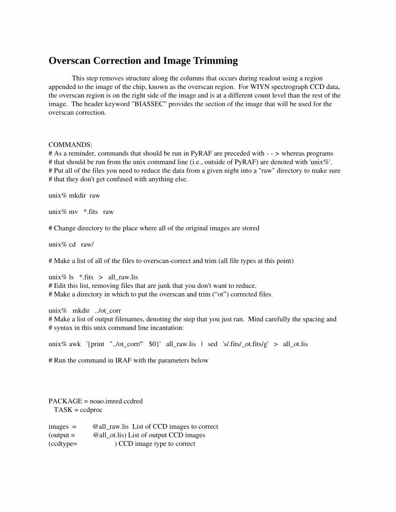
Overscan Correction and Image Trimming

This step removes structure along the columns that occurs during readout using a region appended to the image of the chip, known as the overscan region.  For WIYN spectrograph CCD data, the overscan region is on the right side of the image and is at a different count level than the rest of the image.  The header keyword "BIASSEC" provides the section of the image that will be used for the overscan correction.  

COMMANDS:# As a reminder, commands that should be run in PyRAF are preceded with ­ ­ > whereas programs # that should be run from the unix command line (i.e., outside of PyRAF) are denoted with 'unix%'.# Put all of the files you need to reduce the data from a given night into a "raw" directory to make sure# that they don't get confused with anything else.

unix% mkdir  raw

unix% mv   *.fits   raw

# Change directory to the place where all of the original images are stored

unix% cd   raw/

# Make a list of all of the files to overscan­correct and trim (all file types at this point)

unix% ls   *.fits   >   all_raw.lis# Edit this list, removing files that are junk that you don't want to reduce.# Make a directory in which to put the overscan and trim (“ot”) corrected files.

unix%   mkdir   ../ot_corr# Make a list of output filenames, denoting the step that you just ran.  Mind carefully the spacing and# syntax in this unix command line incantation:

unix% awk   '{print   "../ot_corr/"   $0}'   all_raw.lis   |   sed   's/.fits/_ot.fits/g'   >   all_ot.lis

# Run the command in IRAF with the parameters below

                                                 PACKAGE = noao.imred.ccdred   TASK = ccdproc

images  =         @all_raw.lis  List of CCD images to correct(output =          @all_ot.lis) List of output CCD images(ccdtype=                     ) CCD image type to correct

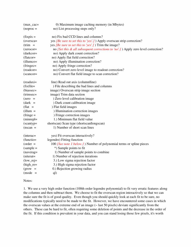
(max_cac=                    0) Maximum image caching memory (in Mbytes)(noproc =                   no) List processing steps only?

(fixpix =                   no) Fix bad CCD lines and columns?(oversca=                yes [Be sure to set this to 'yes'.] ) Apply overscan strip correction?(trim   =                  yes [Be sure to set this to 'yes'.] ) Trim the image?(zerocor=                   no [Set this & all subsequent corrections to 'no'.] ) Apply zero level correction?(darkcor=                   no) Apply dark count correction?(flatcor=                   no) Apply flat field correction?(illumco=                   no) Apply illumination correction?(fringec=                   no) Apply fringe correction?(readcor=                   no) Convert zero level image to readout correction?(scancor=                   no) Convert flat field image to scan correction?

(readaxi=                 line) Read out axis (column|line)(fixfile=                     ) File describing the bad lines and columns(biassec=                image) Overscan strip image section(trimsec=                image) Trim data section(zero   =                     ) Zero level calibration image(dark   =                     ) Dark count calibration image(flat   =                     ) Flat field images(illum  =                     ) Illumination correction images(fringe =                     ) Fringe correction images(minrepl=                   1.) Minimum flat field value(scantyp=            shortscan) Scan type (shortscan|longscan)(nscan  =                    1) Number of short scan lines

(interac=                  yes) Fit overscan interactively?(functio=             legendre) Fitting function(order  =                  100 [See note 1 below.] ) Number of polynomial terms or spline pieces(sample =                    *) Sample points to fit(naverag=                    1) Number of sample points to combine(niterat=                    1) Number of rejection iterations(low_rej=                   3.) Low sigma rejection factor(high_re=                   3.) High sigma rejection factor(grow   =                   0.) Rejection growing radius(mode   =                   ql)

Notes:

1.  We use a very high order function (100th order legendre polynomial) to fit very erratic features alongthe columns and then subtract them.  We choose to fit the overscan region interactively so that we can make sure the fit is of good quality.  Even though you should quickly look at each fit to be sure, no modifications typically need to be made to the fit.  However, we have encountered some cases in which the overscan values at the extreme end of an image (~ last 50 pixels) deviate significantly from the others.  These can be hard to fit, often requiring some deletion of points and the decrease in the order of the fit.  If this condition is prevalent in your data, and you can stand losing those few pixels, it's worth 

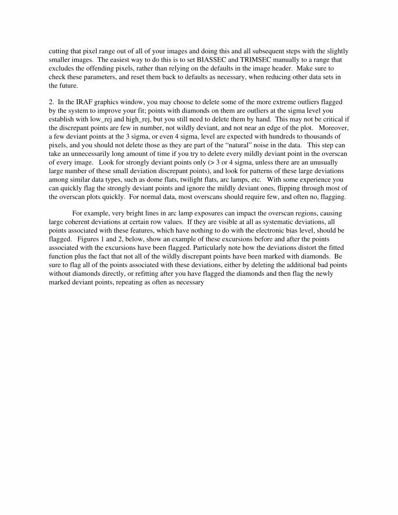
cutting that pixel range out of all of your images and doing this and all subsequent steps with the slightlysmaller images.  The easiest way to do this is to set BIASSEC and TRIMSEC manually to a range that excludes the offending pixels, rather than relying on the defaults in the image header.  Make sure to check these parameters, and reset them back to defaults as necessary, when reducing other data sets in the future.   

2.  In the IRAF graphics window, you may choose to delete some of the more extreme outliers flagged by the system to improve your fit; points with diamonds on them are outliers at the sigma level you establish with low_rej and high_rej, but you still need to delete them by hand.  This may not be critical ifthe discrepant points are few in number, not wildly deviant, and not near an edge of the plot.   Moreover,a few deviant points at the 3 sigma, or even 4 sigma, level are expected with hundreds to thousands of pixels, and you should not delete those as they are part of the “natural” noise in the data.   This step can take an unnecessarily long amount of time if you try to delete every mildly deviant point in the overscan of every image.   Look for strongly deviant points only (> 3 or 4 sigma, unless there are an unusually large number of these small deviation discrepant points), and look for patterns of these large deviations among similar data types, such as dome flats, twilight flats, arc lamps, etc.   With some experience you can quickly flag the strongly deviant points and ignore the mildly deviant ones, flipping through most of the overscan plots quickly.  For normal data, most overscans should require few, and often no, flagging. 

For example, very bright lines in arc lamp exposures can impact the overscan regions, causing large coherent deviations at certain row values.  If they are visible at all as systematic deviations, all points associated with these features, which have nothing to do with the electronic bias level, should be flagged.   Figures 1 and 2, below, show an example of these excursions before and after the points associated with the excursions have been flagged. Particularly note how the deviations distort the fitted function plus the fact that not all of the wildly discrepant points have been marked with diamonds.  Be sure to flag all of the points associated with these deviations, either by deleting the additional bad points without diamonds directly, or refitting after you have flagged the diamonds and then flag the newly marked deviant points, repeating as often as necessary  

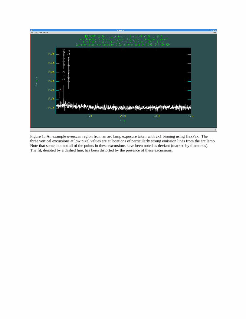
Figure 1. An example overscan region from an arc lamp exposure taken with 2x1 binning using HexPak. The three vertical excursions at low pixel values are at locations of particularly strong emission lines from the arc lamp.Note that some, but not all of the points in these excursions have been noted as deviant (marked by diamonds). The fit, denoted by a dashed line, has been distorted by the presence of these excursions.

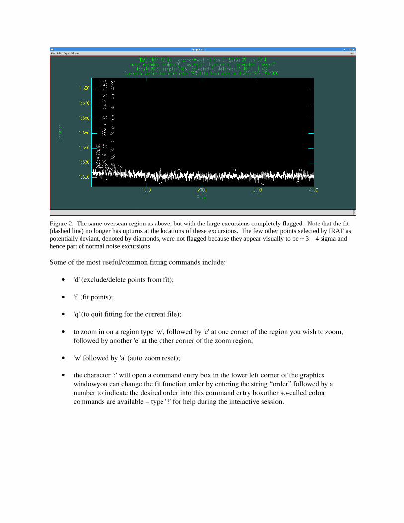
Figure 2. The same overscan region as above, but with the large excursions completely flagged. Note that the fit (dashed line) no longer has upturns at the locations of these excursions. The few other points selected by IRAF as potentially deviant, denoted by diamonds, were not flagged because they appear visually to be ~ 3 – 4 sigma and hence part of normal noise excursions.

Some of the most useful/common fitting commands include:    

'd' (exclude/delete points from fit); 

'f' (fit points); 

'q' (to quit fitting for the current file); 

to zoom in on a region type 'w', followed by 'e' at one corner of the region you wish to zoom, followed by another 'e' at the other corner of the zoom region; 

'w' followed by 'a' (auto zoom reset); 

the character ':' will open a command entry box in the lower left corner of the graphics windowyou can change the fit function order by entering the string “order” followed by a number to indicate the desired order into this command entry boxother so­called colon commands are available – type '?' for help during the interactive session. 

Overview of Combining Similar Spectra

Typically a number of similar exposures are combined into a single 2­D image.  These include bias frames, dark exposures, various types of flat field exposures, and in some cases observations of objects in the sky.  This is done to increase S/N and remove cosmic rays, bad pixels, etc.  Use the IRAF task imcombine to accomplish this.  We have found that it may not be effective to combine several 2­D observations of long exposure science program objects.  See the next section for further discussion of cosmic­ray cleaning when image stacking isn't effective.   

If your images within a group of similar exposures (e.g., zeros, flats, etc.) have differing signal levels you should consider scaling, or applying an additive offset to, the individual images to bring themto a common level before combining them.  Variations in overall image level are frequent occurrences due to variations in exposure time, sky conditions, flat field lamp brightness, or detector electronics.  Adjusting for even relatively small offsets can aid in the rejection of bad pixels and cosmic rays.  Larger than expected offsets can alert you to potential trouble, such as unstable electronics in the case of zeros or a flaky lamp in the case of dome flats.  Twilight flats unavoidably will be very different from each other and so will require large scale factors.   Generally the most effective statistic to use for scaling or applying additive offsets is the median or mode.   Another option, if you are sure that the differences in image scaling results only from different exposure times, and not any other factors, then you can tell IRAF to use the exposure time keyword (EXPTIME) in the file headers to scale the images.   Finally, if none of the above are appropriate, you can set any scale factors you want by entering the numbers in a file, one line at a time and in the same order as the list of input files.  If the name of this file is object_scales.txt, for example, then enter “@object_scales.txt” for the scale parameter in the PyRAF/IRAF imcombine task.  

If the signal levels are significantly different, such as with twilight flats, you should apply weights to each frame to reduce the influence of lower signal and noisier images.  Typically it is not necessary to weight zeros, darks, or dome flats, as the individual frames usually are quite similar to eachother (within a percent or so).  As with scale factors, you can weight by the mean, median, mode, exposure times or by values in a user supplied file.

The image scaling, zero point offsets, and weights will be calculated over a region of the image designated by the 'statsec' parameter.  If this is left blank, imcombine defaults to using the entire image.  In general observers may choose to restrict the statsec to the portion of the image that avoids undesireable features (e.g., bad and variable pixels near the edge of the ccd, or regions of no illumination).   Some people routinely exclude a few pixels around all of the edges from the statsec1.  Data that contain signal from a light source (flats, celestial targets, etc.) present a special complication due to the alternating light and dark regions.  See Appendix E for further discussion.  It is likely that the best approach is to either use the statsec above but select “average” for all statistics (e.g., scaling and weights), in which case one is more susceptible to outliers; or use the more robust “median” or “mode” 

1

For example, with SparsePak and the CCD binned 4x3 we have often used [45:610,15:1320] for a nearly full-frame statsec. However, do not automatically use this statsec for any data, as this section will not be correct for data from different IFUs and / or binning. You must evaluate each data set separately for the correct statsec.

with a statsec that is restricted to the region around a single fiber's spectrum2.  Which of these approaches is best may vary from one situation to another and should be the subject of some investigation.  

In many cases it is possible and desirable to identify and remove unstable pixels and those affected by cosmic rays while combining similar images.  Use this approach whenever it is effective, as it is easier and faster than removing cosmic rays on individual images.  Situations in which cosmic ray removal during image combination may not work well include:  there are only a few images to combine,and you do not have a sufficiently accurate model of the noise; the individual frames are quite different from each other, as can happen with twilight sky flats and sometimes long exposure science observations; or you simply don't wish to combine your images for other reasons.  Removing cosmic rays while combining images can be tricky to do well, and it is easy to remove a lot of real data without realizing it if regions of the images vary by more than is expected from the statistical model assumed in the selected clipping method.   This problem could greatly reduce the S/N of your final result.  One of the best defenses against this is to set the imcombine parameter 'nkeep' to a sensible value.  The best value for nkeep should be the subject of experiment; as a rule of thumb, do not set this parameter to a value below 2/3 of the total number of images (assuming the number to be combined is > 2).  

It is also imperative that you carefully check the diagnostics that can be produced each time you combine a set of images.  The PyRAF/IRAF task imcombine provides the option to create detailed diagnostics of the cosmic­ray rejection process.  The more specialized combining tasks, such as flatcombine, zerocombine, and darkcombine, which are based on the noao.imred.ccdred.combine task, do not offer this option.  Hence, it is important to use imcombine for all image combinations.  

The most important of these diagnostics is enabled by entering a file name for the imcombine parameter nrejmasks.  This will save a single 2­D image with the same number of pixels as exist in each of the input images.  This image is a pixel list file, in which integers represent the number of values the imcombine routine has rejected at each pixel.  For example, if 10 images are combined, a value of 3 at a given pixel means that 3 of the 10 values available at that pixel were rejected.  The minimum value in this pixel list image is 0 and the maximum value should not exceed the number of input images minus the value of the 'nkeep' parameter.  This output file is very useful for quickly diagnosing many problems with pixel rejection in imcombine, and its routine use is strongly recommended.  The result of pixel flagging can vary significantly from one set of images to another.  

Start evaluating the pixel list file containing the number of rejected values by using the PyRAF/IRAF task imstat.  First set the “fields” parameter in imstat to the following string for a good general purpose listing of image statistics: image,npix,mean,midpt,mode,stddev,min,max .  In particular,look at the maximum value.  Is it as high as the maximum number of values which could have been rejected in any pixel (number of images combined minus the value you selected for the nkeep parameter), or did the imcombine task not have to go that high?  Most pixels should not have had any values rejected, so the average over the image should be <~ 1.  Next display the pixel list file.  You cannot display a pixel list file in the normal way with ds9 by itself (using the file open menu operation). Use the PyRAF/IRAF task display to load the pixel list image into ds9.  To be most effective, turn off the auto scaling in the display task and set the maximum display level to the maximum number of pixels

2 Again, using our SparsePak data 4x3 as an example, a useful single column statsec in some cases has been [364:368,15:1320]. You must select your own region based on inspecting your own data!

which were rejected, as determined from imstat.  Type the following literally, as written, except substitute the approriate names and values for the descriptors in brackets: 

­ ­ > display <pixel list image name> zr­  zs­  z1=0  z2=<max number of rejected pixels>

When prompted for the frame number just enter 1 or whichever frame you prefer.  It is also useful to display in different frames (you can use the regular ds9 file open procedure now) the resulting combinedimage and a few of the original images that went into the combination.  You must carefully consider whether the algorithm succeeded in two different measures: 

1. Did it successfully reject almost all real cosmic rays?  Look at the final combined image for structures that look like cosmic rays; there should be few, if any.  You can get a sense of what real cosmic rays look like by looking at any on­sky data with exposures times > a minute or two.Note that hot pixels which don't vary by much will get through the rejection process and may look like small cosmic rays.  You can check this by looking through a few of the original images.  The constant hot pixels should appear in the same places in the original images, as wellas in the combined image.  As you look through the original images, note any particularly prominent cosmic rays.  The same pattern should also appear in the image of rejected pixels.  

2. Many people stop at the previous step without considering that their data might have been subjected to over­cleaning, which is potentially worse than under­cleaning the cosmic rays.  Unlike under­cleaning, over­cleaning may not be obvious in the combined image.  The image may look wonderful, but you may have lost S/N without realizing it.  The quickest way to look for over­cleaning is to study the rejected pixel image.  Do you see many pixels in which the number of rejected values is larger than you expect, based on your rejection threshold and the number of images combined?  Do you see patterns of rejected pixels that look like real features in your data, such as sky lines, the dispersed light from real objects, etc.?  If you encounter suchissues then you likely have a problem and should adjust the rejection parameters (for example, lsigma and hsigma) and try again.  

If you remain baffled by problems with cosmic­ray rejection, you can select an option in imcombine to record every pixel rejected in each of the input files.  By entering a file name in the 'rejmask' parameter, you will trigger IRAF to save an image stack in which each plane is a 2­D image containing the same number of pixels as each of the input images.  The first image plane corresponds to the first image in the list, etc.  Each of these 2­D images is a “pixel list” image, in which a pixel has a value of 1 if that pixel in the corresponding image was rejected during the combination.  Pixels that werenot rejected have a value of 0 in the pixel list image. Hence, this image stack contains complete information about the pixels rejected by imcombine: you can determine which pixels in which images were rejected.  This can be a large image stack and is often time consuming to analyze. Consequently, electing to receive a rejmask is recommended only if the pixel rejection problems cannot be adequately diagnosed with the simpler nrejmask. 

Another diagnostic image you should routinely create and examine is one containing the r.m.s. of the values in each pixel.  Do this by entering a list of names of files to be created in the “sigmas” parameter, one file for each image in the list of output images.  In typical applications in this guide, thereis only one output image, so there should be only one sigma image listed.  Examine the sigma image in ds9.  If you combined images that were exposed to light, the brighter regions should have higher r.m.s. 

values in the sigma image.   Typical r.m.s. values should be approximately equal to the quadrature sum of the read noise and the Poisson noise from the recorded photons.  The r.m.s. in combinations of bias images should be approximately equal to the read noise alone.  You can examine statistics of the entire sigma image, or rectangular subsections, with the PyRAF/IRAF task imstat.  

Finally, you need to choose from among many different rejection algorithms.  These are detailedby typing “help imcombine” at the PyRAF/IRAF prompt.  Recommended options for this parameter, or guidance on how to choose one, will be given in each of the following sections which make use of the imcombine task. The more commonly used rejection algorithms include: 

ccdclip  This uses the CCD characteristics (read noise and gain) and assumes a Poisson noise model to predict the standard deviation about the central value in each pixel.  Values associated with a particular pixel that are more than lsigma and hsigma times smaller or larger, respectively, than this standard deviation are rejected.  This can be an effective algorithm, and it works with as few as two input values.  However, it can be tricky to get right and can easily go awry.  First, you must have accurate values for read noise and gain.  If there are any systematic variations in the signal beyond basic counting noise, such as changes in the sky condition, source flux, throughput due to telescope flexure, flat lamp variations, unstable electronics, etc., then this method may well cause problems, particularly in terms of over­flagging.  It may be possible to mitigate this effect somewhat by giving a non­zero value to the “snoise” parameter, which boosts the assumed noise by a fixed fraction of the central value.  We don't have much experience with setting this “sensitivity noise” value, and you will need to experiment if you want to try this.  Sometimes you may need to use larger than typical “lsigma” and “hsigma” values to get this to work correctly.  Study the diagnostics described above particularly closely ifyou use this rejection algorithm.  If you can use a different algorithm effectively, it is probably better to do so.  

crreject   This is the same as ccdclip but flags only high values, such as cosmic rays.  The same cautions apply.  

sigclip   This calculates the standard deviations of the values for a given pixel from the data themselves.   This is a simple and often very effective rejection algorithm that typically doesn't require as much thought on your part if you are combining a large number of images.  However,it is very dangerous and will utterly fail if you have only a few images.  Specifically, you must have more images than the maximum of lsigma or hsigma squared.  For example, if you set the rejection at 3 sigma, then you must have more than 9 or 10 images for the algorithm to be able to reject any pixels at all.  It can be demonstrated mathematically that if you have fewer than ~ N2 images, you cannot reject any pixels at the N sigma or greater level.  You can reduce N, but then you run the risk of rejecting too much real data.  It is better to use a different algorithm if you have only a few images.  On the other hand, for biases and dome flats, where you typically have many very similar images, this is probably the rejection algorithm of choice.  

avsigclip   This … needs to be filled in! 

minmax   This will reject a fixed number of values at the low end of the distribution in each pixel and/or a fixed number at the high end.  The number rejected at either end is set by the imcombine parameters “nlow” and “nhigh.”  This is crude rejection algorithm, because it will 

reject the same number of values, regardless of whether the values are deviant or not, from every pixel in the image.  It is handy for quick looks at the data but probably should not be used for final reductions.  

pclip   We do not have much experience with this algorithm. 

COMMANDS: # The example below is general.  It shows all of the parameters associated with the imcombine # task.  You will want to adjust these parameters and run imcombine for each group of frames # that you wish to combine. # # This process will be described specifically and in detail for each of the standard sets of images # (biases, flats, darks) in subsequent sections.  Only parameters which must be adjusted or need # further attention will be listed in those sections. 

# Below is an example of how to select all of the files with image type “object” and place # a list of these images into a file.  Don't actually execute this step right now.  Each section # describing a specific image combination task will suggest a way to construct the input # and output files.  

­ ­ >  hselect  *.fits  $I,IMAGETYP  'yes'  >  all_files.lis

unix%  awk  '$2  ==  "object"  {print $1}'  all_files.lis  >  all_objectcomb.lis# Edit the file all_objectcomb.lis to remove any images you don't want to be combined with # the others, and then run the IRAF task imcombine with '@all_objectcomb.lis' for the input.  # Again, zeros, darks, and flats will have their own incantations for generating input file lists, # as detailed in subsequent sections.  

                                 PACKAGE = images.immatch   TASK = imcombine

input   = @all_[object, comp, or standard]comb.lis  List of images to combineoutput  = [Object, Comp, or Standard].fits  List of output images(headers=                     ) List of header files (optional)(bpmasks=                     ) List of bad pixel masks (optional)(rejmask=   [see discussion above] ) List of rejection masks (optional)(nrejmas=  [see discussion above]  ) List of number rejected masks (optional)(expmask=                     ) List of exposure masks (optional)(sigmas =   [see discussion above] ) List of sigma images (optional)(imcmb  =                   $I) Keyword for IMCMB keywords(logfile=               STDOUT) Log file

(combine=            median) Type of combine operation(reject =             sigclip) Type of rejection

(project=                   no) Project highest dimension of input images?(outtype=                 real) Output image pixel datatype(outlimi=                     ) Output limits (x1 x2 y1 y2 ...)(offsets=                 none) Input image offsets(masktyp=                 none) Mask type(maskval=                    0) Mask value(blank  =                   0.) Value if there are no pixels

(scale  =              median [see note 1 below] ) Image scaling(zero   =                 none [see note 1 below]) Image zero point offset(weight =             none) Image weights(statsec=  [see note 2 below]) Image section for computing statistics(expname=              EXPTIME) Image header exposure time keyword

(lthresh=                INDEF [see note 3 below]) Lower threshold(hthresh=                INDEF [see note 3 below]) Upper threshold(nlow   =                    1) minmax: Number of low pixels to reject(nhigh  =                    1) minmax: Number of high pixels to reject(nkeep  = [see discussion above]) Minimum to keep (pos) or maximum to reject (neg)(mclip  =                  yes) Use median in sigma clipping algorithms?(lsigma =                    [see note 4 below]) Lower sigma clipping factor(hsigma =                   [see note 4 below]) Upper sigma clipping factor(rdnoise =         RDNOISE [see note 5 below] ) ccdclip: CCD readout noise (electrons)(gain   =             GAIN [also see note 5 below]) ccdclip: CCD gain (electrons/DN)(snoise =                   0.) ccdclip: Sensitivity noise (fraction)(sigscal=                  0.1) Tolerance for sigma clipping scaling corrections(pclip  =                 ­0.5) pclip: Percentile clipping parameter(grow   =                   0.) Radius (pixels) for neighbor rejection(mode   =                   ql)

Notes on parameters for imcombine:

1. If the exposure times are different, you might consider entering “exposure” for the scale parameter.  Otherwise, and perhaps even if the exposures are different, consider an empirical scaling such as “median.”  The parameter 'zero' will apply an additive offset to each image if selected.  Generally an additive offset won't be used often, except perhaps when combining bias frames.  If for some reason you decide to apply both scaling and additive offsets, be careful and read the help for imcombine carefully to understand what it's doing in this case.  If you use scaling then pay particular attention to statsec.  You want the statsec to sample the part of the image that is relevant to determining the scale values.  For example, if you’re trying to scale by flux in an object but your statsec contains mostly sky, the scaling won’t work very well.    

2. Parameter 'statsec' indicates the region of the image over which the statistics for image scaling (parameter 'scale') are computed.  See the discussion above.    For bias and dark frames use a nearly full­frame statsec.  Use this same statsec for frames with illumination if you are using 

“average” for all of your statistics (e.g., scaling and weights).  Otherwise, for the illuminated frames use the region around a single fiber.  

3. In many applications of imcombine it's probably fine to leave lthresh and hthresh set to the default values of INDEF (which turns off the thresholding).  Values which are out of range due to bad pixels or cosmic rays should be culled by the clipping algorithm you select without resorting to thresholding.  Turning on thresholding can in principle hide problems from you, since you may not see misbehaving pixels in the rejected pixel files.  It's also possible to toss outall of the values in a pixel and cause an error (preferred in this situation) or have the code substitute a value of its own choosing (not preferred – I'm not sure if this would happen; need to check).  However, in situations where parts of some of the images are deliberately saturated to increase the S/N in another part of the image, as can happen with twilight flat fields, then settingappropriate values for the threshold parameters, and carefully watching the rejections, is essential.  

4. The conventional sigma clipping values (lsigma and hsigma) are 3.  For standard stars and arc lamps you will likely have to increase the parameters lsigma and hsigma to values larger than the canonical 3 sigma (try 4 or 5, higher if needed), to avoid clipping real data such as emission lines.  Check the nrejmask image to look for evidence of clipping real data. These should also beincreased when combining bias frames, as described in the Bias section. 

5. The "rdnoise" and "gain" parameters are set so that the information in the appropriate header keywords are retrieved.  This is the same for all subsequent steps.  Parameter 'rdnoise' normally can be set to the name of the image header key word that lists the read noise (often RDNOISE), but Matt Bershady has found that the value printed in the image headers for the CCD used with the Bench Spectrograph is wrong in some cases.  For example, as of this writing (11 JUL 2012), the read noise according to Bershady is 4.4 electrons for 4x3 binning.  Proper readnoise values for other binnings should be investigated.

Cosmic Ray Removal on Individual Images

Often the best and easiest way to remove cosmic rays from images is with an appropriate selection of clipping algorithm during image combination, as described in the previous section.  However, in some cases, most notably the on­sky data of the program objects (the whole point of the observing run!) and on the twilight sky flats, this may not work well because the sky conditions change too much from one exposure to the next.  It may be possible to effectively remove the cosmic rays by combining pairs of object frames (set the “reject” parameter to crreject or possibly ccdclip and be careful), and then later combining the 1­D spectra after extraction.  Whether this latter approach is effective may change from time to time, even during the same night.  You will have to experiment with the data to see how well the cosmic ray rejection is working.  

If cosmic­ray rejection via 2­D image combining does not work well enough, then the remainingoption is to remove cosmic rays on individual images.  This can be difficult and time consuming.  It takes patience and experimentation to arrive at the correct parameters to remove almost all of the cosmicrays while still retaining real features in the data.  The method we have used primarily to date is the task 'cosmicrays' in the package 'crutil'.   Laplacian edge detection, via a different task, works well for cosmicray removal on images and long­slit data, but it has not been found to work well yet on SparsePak data.  See Appendix E for further discussion.  We are currently experimenting with an alternate task for cosmic ray removal called 'PyCosmic'.  

Task 'cosmicrays'

It is strongly recommended that you enter a file name for the “crmasks” parameter (actually one name for each input image), which will create a pixel list image showing which pixels have been flaggedas cosmic rays.  Examine this, plus the resultant output image carefully, to see how well the task has rejected real cosmic rays and that it has refrained from flagging real data as cosmic rays.  If it is going tooverflag, it will often do so on bright emission lines, such as sky lines.  If the routine is under­ or over­flagging, adjust the flagging parameters.   Much of the discussion regarding diagnosing the efficacy of cosmic­ray rejection in the “Overview on Combining Similar Spectra” section applies here as well. 

PACKAGE = noao.imred.crutilTASK = cosmicrays

input =                              List of images in which to detect cosmic raysoutput =                            List of cosmic ray replaced output images (optional)answer =                           Review parameters for a particular image?(crmasks = [see discussion above] )    List of bad pixel masks (optional)(threshold = 32 [see note 1 below] )               Detection threshold above mean(fluxratio = 15  [see note 2 below] )                Flux ratio threshold (in percent)(npasses = 10   [see note 3 below])                  Number of detection passes(window = 7    [see note 4 below] )                   Size of detection window

(interactive = no)             Examine parameters interactively?(train = no  [see note 5 below] )                        Use training objects?(objects = "")                     Cursor list of training objects(savefile = "")                    File to save train objects(plotfile = "")                     Plot file(graphics = "stdgraph")     Interactive graphics output device(cursor = "")                      Graphics cursor input(mode = "al")           

Notes on parameters for cosmicrays:

1. So far, we have not found the algorithm to be particularly sensitive to the “threshold” parameter.

2. The “fluxratio” is the key parameter.  A higher number for fluxratio  will flag more pixel values.A single number is probably not appropriate for all data sets.  Experiment with a range of valuesfor this parameter, examining the “crmasks” file and the “output” image; blink different crmasksfiles against each other plus blink the crmask against the output image.  Look for both under­ and over­flagging.  

3. We have not yet explored the impact of different values of the “npasses” parameter.  

4. The “window” parameter can take a value of either 5 (5 x 5 window) or 7 (7 x 7 window).  The help for the task describes some factors in choosing one or the other.  We find that 7 often worksbest for Sparsepak data taken for a quasar host project, but experimentation on each data set is encouraged.  Our initial experiments with using the “train” capability in this task did not prove especially useful.  However, we have not explored this in depth.    The training capability might be useful and should be investigated.  

Task 'PyCosmic'

Add a description of PyCosmic, including how to get it and how it fits in with regular PyRAF (if this is extensive put in Appendix C).  

Add a discussion of how to use it, the typical parameter lists and default values.  Here are Marsha's notes on one of her tests:

PyCosmic 24may2009_088dc.fits wolftest.fits wolftest_mask.fits RDNOISE –siglim 12 –fwhm2.0 –rlim 1.0 –iter 6 –replacebox 33

Bias (also known as Zero) Correction

You first need to combine these exposures to reduce noise and then subtract the master bias frame from all of the other frames.  See Appendix B for more information regarding the zero frames.  Remember to frequently check that you are in the correct directory, both in the unix terminal and the PyRAF/IRAF terminal. 

Combine the Zeros

COMMANDS:

# First, make a list of the zero frames that have been OT­corrected, "all_zero.lis" 

unix% cd  ../ot_corr

­ ­ >  hselect  *.fits  $I,IMAGETYP  'yes'  >  all_files.lis# Note that the character after the '$' in the previous line is the capital letter 'I', not the digit representing# the number “one.”  Type this line with the spacing as indicated.  In particular, note that there # are no spaces  between the strings '$I' , 'IMAGETYP' , and the coma separating them.  The spelling of ‘IMAGETYP’ is correct; there is no letter ‘E’ at the end to spell “type.” 

unix%  awk  '$2  ==  "zero"  {print $1}'  all_files.lis  >  all_zeros.lis# Check the contents of the file all_zeros.lis to make sure that it contains all of the zero images # and only the zero images.  As discussed in the introduction, you should have verified the types of # all images and resolved any discrepancies between the image headers and the log sheets.  

Run the imcombine command in PyRAF/IRAF as follows.  Only the parameters which need to be changed from those given in the “Overview of Combining Similar Spectra,” or those which should be inspected every time, are listed.  

                      PACKAGE = images.immatch   TASK = imcombine

input   =   @all_zero.lis ) List of images to combineoutput  =                Zero)  List of output images… (rejmask=  [leave blank unless needed] ) List of rejection masks (nrejmas=  zero_nrejmask  [see note 1 below] ) List of number rejected masks (optional)… (sigmas =  zero_sigma [see discussion in Overview of Combining] ) List of sigma images (optional)… 

(combine=            median) Type of combine operation

(reject =                 sigclip) Type of rejection… 

(scale  =              none  [see note 2 below] ) Image scaling(zero   =              median [see note 2 below]) Image zero point offset(weight =             none) Image weights(statsec =  [see disc. in Overview of Combining]) Image section for computing statistics… 

… (nkeep  = [see disc. in Overview of Combining]) Minimum to keep (pos) or maximum to reject (neg)… (lsigma  =             5 [see note 3 below] ) Lower sigma clipping factor(hsigma =             5 [see note 3 below] ) Upper sigma clipping factor… 

Notes: 

1. Be sure to check the diagnostics, as described in the “Overview of Combining Similar Spectra.” It is likely that you won't find many problems, since zeros are in some sense the simplest images.  However, if there are some electonic stability issues, this is a good place to look for them.  

2. Zeros are expected to vary slightly with time.  This is normally treated as an additive offset; see the discussion of overscan subtraction in the “Overscan Correction and Image Trimming” section.   Hence, typically we use a zero offset rather than a scaling when combining zeros.  Thevariations should be small over the time it takes to record a run of zeros, so the additive offsets reported by imcombine should all be small.  If they're larger than usual, or one or more stand outwith deviant offsets, then you should investigate further.  

3. Zeros should have few, if any, cosmic rays and unstable pixels.  However, it is still worth turning on pixel value rejection just to see if there are any such pixels and how extensive they are.  If they are few and in non­critical places, you can delete the clipped image and remake a non­clipped combined image; or you can keep the one you have.  If you keep the clipped image,you should increase the sigma clipping values (lsigma and hsigma) to a higher value (e.g., to 5) in order to not artificially skew the image statistics by removing many pixels which simply stochastically go above 3 sigma.  You should reset lsigma and hsigma back to the typical value (e.g., 3) after running imcombine on the bias images and before you combine any images in which you expect cosmic rays.  

Apply the Combined Zero to the Other Images

# Now zero/bias­correct all of the rest of the frames.  

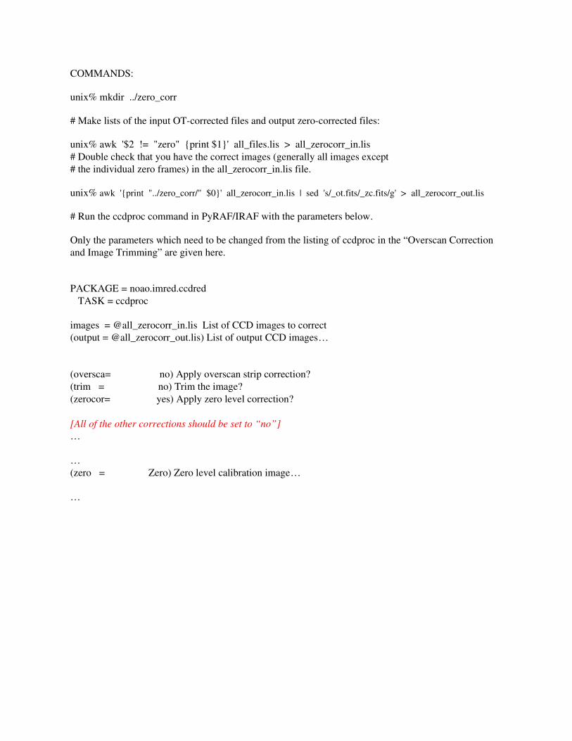
COMMANDS:

unix% mkdir  ../zero_corr

# Make lists of the input OT­corrected files and output zero­corrected files:

unix% awk  '$2  !=  "zero"  {print $1}'  all_files.lis  >  all_zerocorr_in.lis# Double check that you have the correct images (generally all images except # the individual zero frames) in the all_zerocorr_in.lis file. 

unix% awk  '{print  "../zero_corr/"  $0}'  all_zerocorr_in.lis  |  sed  's/_ot.fits/_zc.fits/g'  >  all_zerocorr_out.lis

# Run the ccdproc command in PyRAF/IRAF with the parameters below.

Only the parameters which need to be changed from the listing of ccdproc in the “Overscan Correction and Image Trimming” are given here.  

                                       PACKAGE = noao.imred.ccdred   TASK = ccdproc

images  = @all_zerocorr_in.lis  List of CCD images to correct(output = @all_zerocorr_out.lis) List of output CCD images… 

(oversca=                   no) Apply overscan strip correction?(trim   =                     no) Trim the image?(zerocor=                  yes) Apply zero level correction?

[All of the other corrections should be set to “no”]… 

… (zero   =                 Zero) Zero level calibration image… 

… 

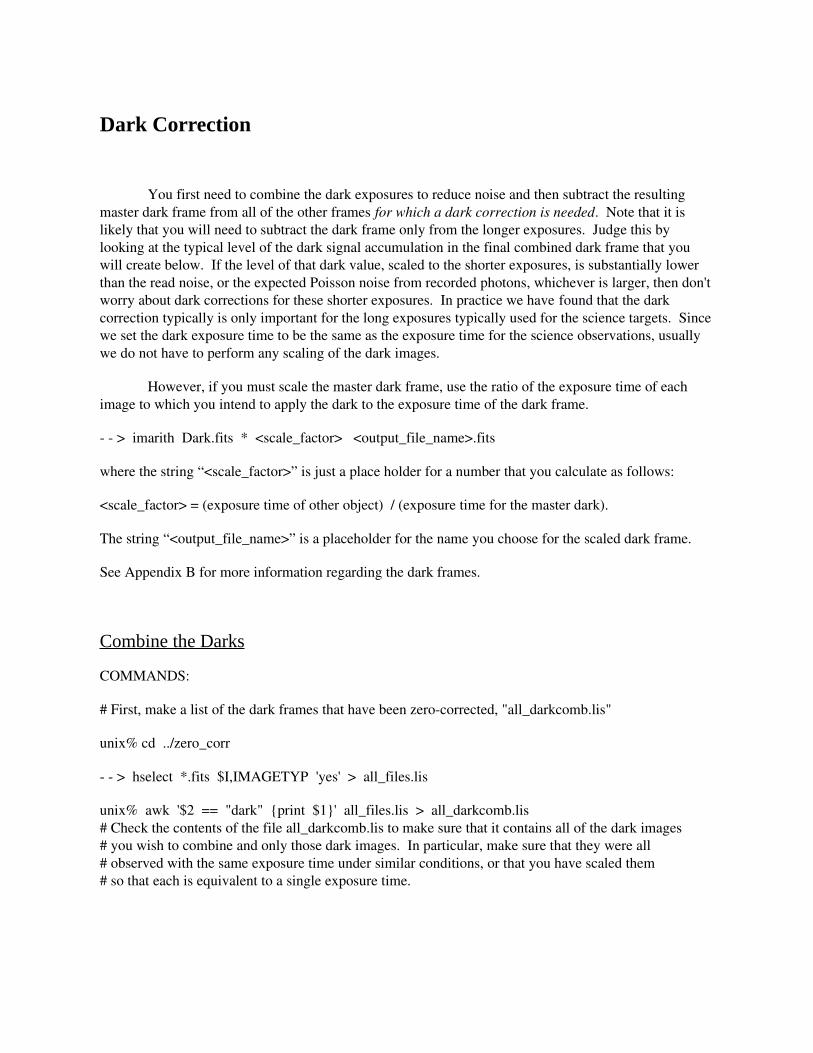
Dark Correction

You first need to combine the dark exposures to reduce noise and then subtract the resulting master dark frame from all of the other frames for which a dark correction is needed.  Note that it is likely that you will need to subtract the dark frame only from the longer exposures.  Judge this by looking at the typical level of the dark signal accumulation in the final combined dark frame that you will create below.  If the level of that dark value, scaled to the shorter exposures, is substantially lower than the read noise, or the expected Poisson noise from recorded photons, whichever is larger, then don'tworry about dark corrections for these shorter exposures.  In practice we have found that the dark correction typically is only important for the long exposures typically used for the science targets.  Sincewe set the dark exposure time to be the same as the exposure time for the science observations, usually we do not have to perform any scaling of the dark images.

However, if you must scale the master dark frame, use the ratio of the exposure time of each image to which you intend to apply the dark to the exposure time of the dark frame.  

­ ­ >  imarith  Dark.fits  *  <scale_factor>   <output_file_name>.fits

where the string “<scale_factor>” is just a place holder for a number that you calculate as follows: 

<scale_factor> = (exposure time of other object)  / (exposure time for the master dark). 

The string “<output_file_name>” is a placeholder for the name you choose for the scaled dark frame. 

See Appendix B for more information regarding the dark frames.   

Combine the Darks

COMMANDS:

# First, make a list of the dark frames that have been zero­corrected, "all_darkcomb.lis" 

unix% cd  ../zero_corr

­ ­ >  hselect  *.fits  $I,IMAGETYP  'yes'  >  all_files.lis

unix%  awk  '$2  ==  "dark"  {print  $1}'  all_files.lis  >  all_darkcomb.lis# Check the contents of the file all_darkcomb.lis to make sure that it contains all of the dark images # you wish to combine and only those dark images.  In particular, make sure that they were all # observed with the same exposure time under similar conditions, or that you have scaled them # so that each is equivalent to a single exposure time.  

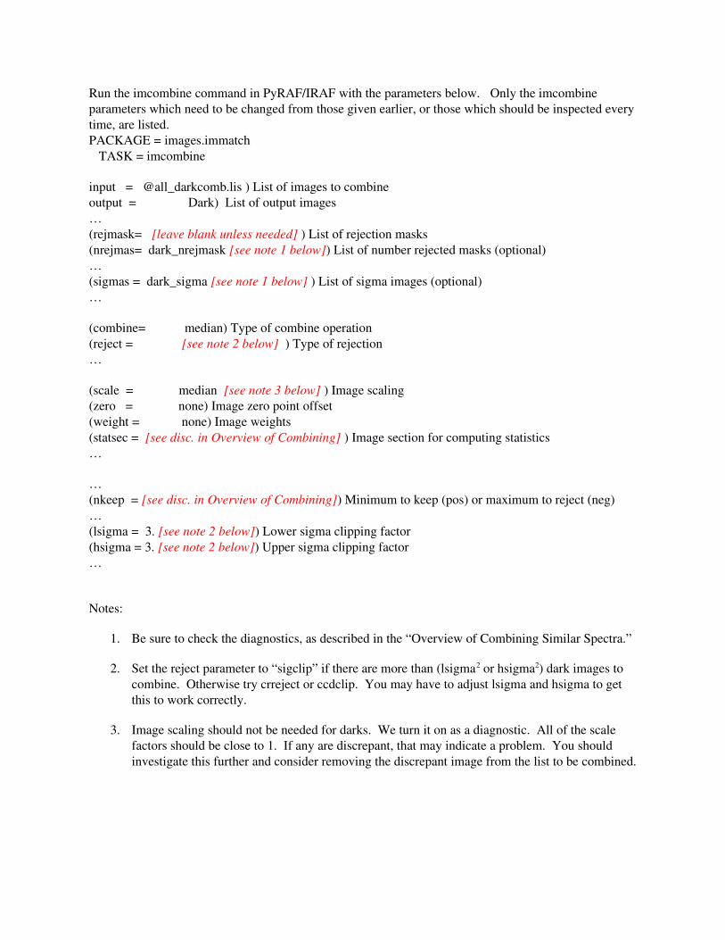
Run the imcombine command in PyRAF/IRAF with the parameters below.   Only the imcombine parameters which need to be changed from those given earlier, or those which should be inspected everytime, are listed.  PACKAGE = images.immatch   TASK = imcombine

input   =   @all_darkcomb.lis ) List of images to combineoutput  =                Dark)  List of output images… (rejmask=   [leave blank unless needed] ) List of rejection masks (nrejmas=  dark_nrejmask [see note 1 below]) List of number rejected masks (optional)… (sigmas =  dark_sigma [see note 1 below] ) List of sigma images (optional)… 

(combine=            median) Type of combine operation(reject =               [see note 2 below]  ) Type of rejection… 

(scale  =              median  [see note 3 below] ) Image scaling(zero   =              none) Image zero point offset(weight =             none) Image weights(statsec =  [see disc. in Overview of Combining] ) Image section for computing statistics… 

… (nkeep  = [see disc. in Overview of Combining]) Minimum to keep (pos) or maximum to reject (neg)… (lsigma =  3. [see note 2 below]) Lower sigma clipping factor(hsigma = 3. [see note 2 below]) Upper sigma clipping factor… 

Notes: 

1. Be sure to check the diagnostics, as described in the “Overview of Combining Similar Spectra.” 

2. Set the reject parameter to “sigclip” if there are more than (lsigma2 or hsigma2) dark images to combine.  Otherwise try crreject or ccdclip.  You may have to adjust lsigma and hsigma to get this to work correctly.  

3. Image scaling should not be needed for darks.  We turn it on as a diagnostic.  All of the scale factors should be close to 1.  If any are discrepant, that may indicate a problem.  You should investigate this further and consider removing the discrepant image from the list to be combined.

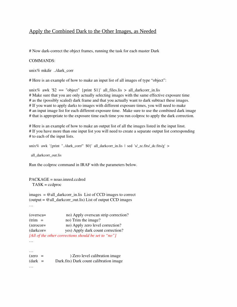
Apply the Combined Dark to the Other Images, as Needed

# Now dark­correct the object frames, running the task for each master Dark

COMMANDS:

unix% mkdir  ../dark_corr

# Here is an example of how to make an input list of all images of type “object”:

unix%  awk  '$2  ==  "object"  {print  $1}'  all_files.lis  >  all_darkcorr_in.lis# Make sure that you are only actually selecting images with the same effective exposure time # as the (possibly scaled) dark frame and that you actually want to dark subtract these images.  # If you want to apply darks to images with different exposure times, you will need to make # an input image list for each different exposure time.  Make sure to use the combined dark image # that is appropriate to the exposure time each time you run ccdproc to apply the dark correction. 

# Here is an example of how to make an output list of all the images listed in the input linst. # If you have more than one input list you will need to create a separate output list corresponding # to each of the input lists.  

unix%  awk  '{print  "../dark_corr/"  $0}'  all_darkcorr_in.lis  |  sed  's/_zc.fits/_dc.fits/g'  >

  all_darkcorr_out.lis

Run the ccdproc command in IRAF with the parameters below.

PACKAGE = noao.imred.ccdred   TASK = ccdproc

images  = @all_darkcorr_in.lis  List of CCD images to correct(output = @all_darkcorr_out.lis) List of output CCD images… 

(oversca=                   no) Apply overscan strip correction?(trim   =                     no) Trim the image?(zerocor=                   no) Apply zero level correction?(darkcor=                  yes) Apply dark count correction?[All of the other corrections should be set to “no”]… 

… (zero   =                         ) Zero level calibration image(dark   =           Dark.fits) Dark count calibration image… 

…

Combine the Flats

See Appendix B for more information regarding the flat frames. 

For each instrument configuration and each night, combine the individual dome flats into a master dome flat and the sky flats (if you have them) into a separate master sky flat (i.e., don't combine sky flats and dome flats together into the same final image).  For dome flats, carefully check your individual flat images to make sure that no parts of them (except for hot pixels and cosmic rays, which can't be helped) exceed the linearity limits of the CCD.  For the current Sparsepak CCD we try to stay below 150000 counts.  Check these by displaying a flat image, identifying the brightest regions, and then plot the dispersion direction with the task imexam ('c' plots a column) or plot across the fibers ('l' plots a line).  This is usually pretty straightforward with dome flats, as the lamp levels and exposure times almost always stay the same during a sequence of flat exposures.  Typically you can check just a few dome flats to make sure that they are below the onset of non­linearity and then combine all of them together into a master flat, as shown below in the listing of parameters for the task flatcombine.  However, the process, while similar in concept, is a little more involved with twilight flats; this will be described separately later in this section.  

Combine the Dome Flats

COMMANDS:# First, make a list of the flat frames that have been zero corrected, "all_domeflatcomb.lis".  # You probably didn't need to dark correct these flats given their generally short exposure times, # but if you did need to dark correct them, then use an appropriately scaled dark frame.  If # you did dark correct them, they may not be in the zero_corr directory as indicated below: 

unix% cd  ../zero_corr# Run the commands below for each group of flats that you are combining (e.g. for each configuration# or pointing).  In particular, combine dome flats separately from sky flats. # Make sure that the files listed in all_domeflatcomb.lis consist of only the dome flats.  If the observer# set the image type of the sky flats to “flat” these sky flats also will be in this list file; you must remove # them in that case.  

unix%  awk  '$2  ==  "flat"  {print  $1}'  all_files.lis  >  all_domeflatcomb.lis

Run the imcombine command in PyRAF/IRAF with the parameters below.   Only the imcombine parameters which need to be changed from those given earlier or those which should be inspected every time are listed.  PACKAGE = images.immatch   TASK = imcombine

input   =   @all_domeflatcomb.lis ) List of images to combine

output  =                Domeflat )  List of output images… (rejmask= [leave blank unless needed] ) List of rejection masks (nrejmas=  domeflat_nrejmask [see note 1 below] ) List of number rejected masks (optional)… (sigmas =  domeflat_sigma [see note 1 below] ) List of sigma images (optional)… 

(combine=            median [but see note 2 below if you apply weights] ) Type of combine operation(reject =               [see note 3 below]  ) Type of rejection… 

(scale  =              median  [see note 4 below] ) Image scaling(zero   =              none) Image zero point offset(weight =             none [see note 2 below] ) Image weights(statsec =   [see disc. in Overview of Combining]) Image section for computing statistics… 

… (nkeep  =  [see disc. in Overview of Combining]) Minimum to keep (pos) or maximum to reject (neg)… (lsigma =  3. [see note 3 below]) Lower sigma clipping factor(hsigma = 3. [see note 3 below]) Upper sigma clipping factor

Notes: 

1. Be sure to check the diagnostics, as described in the “Overview of Combining Similar Spectra.” 

2. Normally you do not need to bother weighting the dome flats if the scale factors are close to 1.  If this is not the case, then look into applying weights. If you apply weights, then you will have to set the “combine” algorithm to average. 

3. Set the reject parameter to “sigclip” if there are more than (lsigma2 or hsigma2) dome flat imagesto combine.  Otherwise try crreject or ccdclip.  You may have to adjust lsigma and hsigma, probably to larger values such as 4 or 5, to get this to work correctly.  

4. You may see modest variations in the scale factors for dome flats due to variations in the lamp intensity.  If the variations are large (more than 10 percent?), look into the situation more closely.  In this case you might consider changing the “combine” algorithm from median to average. 

Combine the Twilight Sky Flats

Making a good master twilight sky flat is not as straightforward as the dome flat, but it is very important because the twilight flats are used later to trace the extent of the spectrum in each fiber and to 

perform the relative flux calibration from one fiber to the next, particularly for blue spectra.  The illumination level of twilight flats can vary substantially between one flat and the next, because the brightness of the sky, as well as its spectral shape, changes very rapidly as the sun sets or rises.  We adjust the exposure times while observing to try to roughly keep up with this variation.  Consequently you have to check more carefully whether the linearity range of the detector3 is exceeded in each flat.  

Look through the individual twilight flat field images.  If you see one or more fibers which appear differently, relative to the other fibers in the same image, and based on comparing them to how these same fibers appear in most of the other images, then you may have starlight contamination in the fibers which appear to be different.  This starlight contamination may hamper the fiber­to­fiber relative flux calibration.  You should note which fibers in which images are affected.  If the number of affected images are few in number, it may be easiest to simply exclude these from the list of twilight flats to be combined.  However, if you decide that you need some of the affected images, it may be worth masking out the contaminated fibers in these images.  (Does imcombine let us do that?  If not, we may have to make a copy of these images and set the bad regions to zero.  Investigate.)

There are at least three approaches to making a master twilight flat, though one is deprecated.  Cleaning cosmic rays from each individual file in advance is essential for method 3 and may be useful, or even essential in some cases, for the others.   

1. Our current approach uses all or nearly all of the individual twilight flat frames which have at least some pixels with values less than the non­linearity threshold. It is possible to use twilight flats in which part of the spectra exceed the linearity threshold, or even the saturation threshold if there isn’t charge bleeding, by setting the hthreshold parameter in the task imcombine to a value that is below the linearity limit (see Appendix D on the CCD characteristics).  Be careful of setting this threshold too low, or else you may end up with no data in parts of the spectrum (likely the red end).  Careful examination of your data and an appropriate selection of the hthreshold parameter are very important.  The task will automatically cull any values above this threshold.  This feature can be useful for blue setups, in which it is difficult to get sufficient S/N in the blue without saturating the red. You can take several twilight flats with high S/N in the blue but in which the red is non­linear or saturated and then several more in which the red and intermediate wavelengths are in the linear regime.   The images should be weighted by their original fluxes so that flats with much less illumination can contribute something to the combination without unduly raising the noise.  It doesn't matter in the simplest mathematical sense (see Appendix E) whether the twilight spectra have the same shape, since each different image will receive the same input spectrum into each fiber.  We only need to preserve the ratio of the flux in one fiber to another, and the total cumulative light source feeding all of the fibers is in principle irrelevant (as long as there is enough S/N at all wavelengths).   In order to have any hope of flagging cosmic rays or stellar contamination, we probably need to scale the variousspectra so that they are roughly at the same flux scale.  In order to use weights, we need to combine with “average,” not “median” or “mode.” Hopefully the averaging of several exposures, plus weighting, will sufficiently beat down the contribution of any remaining contaminating star light or cosmic rays in the final master twilight flat.  

3

See Appendix D, on the characteristics of the CCD used in the Bench Spectrograph, for a discussion of detector non-linear and saturation thresholds.

2. Perhaps the best approach, which will take some coding and so won't be available for a while, would be to apply approach 1, then cycle back through each individual flat to compare the relative fiber­to­fiber ratios to those in the combined flat.  Any fiber that deviated more than expected, given the noise, would be excluded from the next version of the master flat.  A new combined flat would be created, followed by another round of individual comparisons, until the method converged (no new exclusions). 

3. Our old approach, now deprecated, was to look through all of the twilight flats which do not exceed the linearity threshold to find two or three (more if possible, but that's less likely) that have peak values below the linearity threshold and have similar spectral shapes.  Then combine just these few images using imcombine.  Be sure to set nkeep = 1 or else you may throw away a large portion of your data, thereby dropping the S/N in your twilight flat without realizing it.  It is very important that you try to exclude any images with noticeable star light in any of the fibers.   

Make a file called all_skyflatcomb.lis which lists all of the twilight sky images you wish to combine.  It may be easiest to do this by hand, especially if you are combining only a few of the ones you observed.  

Finally, combine the twilight sky flats using imcombine, as indicated below.  

PACKAGE = images.immatch   TASK = imcombine

input   =   @all_skyflatcomb.lis ) List of images to combineoutput  =                Skyflat )  List of output images… (rejmask=   [leave blank unless needed] ) List of rejection masks (nrejmas=  skyflat_nrejmask [see note 1 below]) List of number rejected masks (optional)… (sigmas =  skyflat_sigma [see note 1 below] ) List of sigma images (optional)… 

(combine=            average ) Type of combine operation(reject =               [see note 2 below]  ) Type of rejection… 

(scale  =                [see note 3 below] ) Image scaling(zero   =              none) Image zero point offset(weight =             [see note 4 below] ) Image weights(statsec =  [364:368,15:1320]   [see note 4 below]) Image section for computing statistics

… 

(lthresh  =            INDEF  ) Lower threshold(hthresh =            [see note 5 below] ) Upper threshold… 

(nkeep  = [see disc. in Overview of Combining]) Minimum to keep (pos) or maximum to reject (neg)… (lsigma =  3. [see note 2 below]) Lower sigma clipping factor(hsigma = 3. [see note 2 below]) Upper sigma clipping factor

Notes: 

1. Be sure to check the diagnostics, as described in the “Overview of Combining Similar Spectra.” 

2. If you are combining only two or three twilight flats, you will likely need to clean the cosmic rays from the individual images first, as described in the “Cosmic Ray Removal” section.  In this case, set the reject parameter to “none”.  You could also try to reject cosmic rays during the image combining by setting the reject parameter to “crreject” (you may have to experiment with lsigma and hsigma).  Be careful with this, and don't be surprised if it doesn't work well.  If you are combining many flats, you still will probably have to clean the cosmic rays from them individually.  If you try to flag cosmic rays from many twilight flats during the combination, try “sigclip” for the reject parameter if you have enough images.      

3. Scaling by the median is probably best, but this should be the subject of some experimentation.  In particular, compare this result to that from not scaling at all.  (If you don't scale, then cosmic ray rejection using imcombine is hopeless, and you should set reject to “none.”)

4. Weights should be enabled.  It is not clear yet which is the optimal weighting scheme to use (mean, median, or mode) and over which statsec these should be computed.  See the Overview of Combining Similar Spectra for further discussion of the 'statsec'.   This needs to be the subjectof some experimentation.  Start with median or mode.  Check to make sure the weights are calculated before the scaling.  If not, then don't scale.  If they are, it'd still be prudent to try a testin which the twilight flats are scaled and in which they are not; then compare the throughput corrections derived from each of these.  

5. If you are combining any twilight flats which approach or exceed the linearity value, set hthresh to a number a little below the linearity threshold.  See the discussion of linearity and saturation thresholds in Appendix D on the Bench Spectrograph characteristics.  If none of your flats are expected to be near this level, then you can leave this at INDEF as it has been before.  

Neither the dome flat nor the twilight flat will be used in another execution of ccdproc, as we did for the previous calibrations.  Rather, they will be used as part of the dohydra task and later for fiber­to­fiber throughput corrections, both described further on in this document.  

Combine Other Similar Sets of Data

Other types of images you may wish to combine include sequences of arc calibration lamp exposures, sequences of standard star exposures, and sequences of observations of the scientific targets of the observing run.  The motivations for doing this include removing cosmic rays and boosting S/N.  Be sure to combine only sequences of exposures that were taken one after another.  Do not combine groups of calibration exposures taken at different times into a single image.  Flux calibration, atmospheric conditions, and possibly wavelength calibration, are time dependent.  You want separate combined images for each group of the calibration exposures so that you can track the temporal variations.   It's an open question as to how many of the science exposures you can effectively combine at once.  This depends heavily on how long the exposures are and how quickly the airmass and atmospheric conditions were changing.  In practice, we have found that typically it is not effective to combine more than two 30­minute exposures, and sometimes it is better to keep all of the science exposures separate for some targets.  

It may be that in some cases you will decide not to combine images in one of these sequences.  There may be too few images in a sequence for effective cosmic ray removal, perhaps the sky conditionswere changing too rapidly for science target or standard star observations, or the emission line lamp was not sufficiently stable in brightness during sequences of wavelength calibration exposures.  Look at eachsequence of exposures to see how much variation there is within the sequence.  You may simply need to try combining the sequence to see how it works.  Don't forget to pay close attention to the diagnostics produced by imcombine, as discussed in the “Overview of Combining Similar Spectra” section.  

Below are notes for what yet needs to be written in this section. 

Describe arc calibrations.  May have groups at diff. Exp. Times.  Combine these separately.  If bright lines are saturated, experiment with setting hthresh to the linearity limit (150000); however, may lose all data in the saturated lines.  Experiment. 

Describe standard star combinations.  Base this on my conversation with Yifei.  Also only combine standards taken under identical conditions.  For example, don't combine drifted spectra with non­drifted or images taken on different drifts.  

For standard stars and arc lamps you will likely have to increase the parameters lsigma and hsigma to values larger than the canonical 3 sigma, to avoid clipping real data such as emission lines.  Be sure to enter an image name for the nrejmask parameter.  Inspect this image, which shows flagged pixels, to make sure the algorithm is not picking real data.  If it is, try increasing the value of lsigma and hsigma. 

Extract Spectra from the Fibers (DOHYDRA)

Once you have a reduced, and possibly stacked, object frame then you need to extract the spectra for each fiber along the dispersion direction (approximately parallel to the columns of the CCD).A helpful companion guide for this task is iraf.net/irafdocs/dohydra.pdf  .  You first must mark the fibersthat you used.  Then you have to trace the fibers, since the column number range of each fiber is a slight function of row number.  You must also determine the dispersion solution for your spectrum.  Note that flatfielding is also done along the way.  For these reasons, this step is done for each pointing.  You may prefer to have a separate directory for each target  where you have copied over, or provided a link to, your stacked comparison lamp, dome flat (or skyflat), and object exposures, read in as "Comp", "Domeflat" or "Skyflat" , and "Object".

If some of your exposures are from different nights, then dohydra will crash at the very end of the process.  See Appendix C for guidance on what to do in this case.  

There are three main parameter files for which you have to check/set parameters.  For the first one below, you probably won't have to change anything, other than possibly the 'dispaxis' parameter.

  

Setting the “hydra” high-level parameters

PACKAGE = noao.imred   TASK = hydra

(observa=          observatory) Observatory of data(interp =                poly5) Interpolation type(dispaxi=                    2   [see note 1 below] ) Image axis for 2D/3D images(nsum   =                    1) Number of lines/columns/bands to sum for 2D/3D images

(databas=             database) Database(verbose=                   no) Verbose output?(logfile=              logfile) Log file(plotfil=                     ) Plot file

(records=                     )(version= HYDRA V1: January 1992)(mode   =                   ql)($nargs =                    0)

Notes: 

1. The 'dispaxis' parameter should be set to 1 if the dispersion axis (direction in the spectral 2­D image corresponding to the wavelength axis) is along image lines; otherwise it should be set to 2

if the dispersion axis is along image columns.  The current (19 JAN 2013)  Bench Spectrograph CCD system places the dispersion along columns.  Many long slit spectrographs place the dispersion axis along lines. 

Setting the “dohydra” task parameters

For this and the subsequent set of parameters, you will need to change/set a number of values, somake sure that you go through them carefully.  This discussion focuses on the extraction of object spectra.  A similar approach will be needed for the twilight sky flats, described in a later section. 

                                            PACKAGE = noao.imred.hydra   TASK = dohydra

objects =               Object  List of object spectra(apref  = Domeflat or Skyflat [see 1. below]) Aperture reference spectrum(flat   = Domeflat  [see 1. below]) Flat field spectrum(through= throughputs.dat [see 1. below]) Throughput file or image (optional)(arcs1  =                 Comp) List of arc spectra(arcs2  =                     ) List of shift arc spectra(arcrepl=                     ) Special aperture replacements(arctabl=                     ) Arc assignment table (optional)

(readnoi=  [see discussion in “Combine the Flats” section]) Read out noise sigma (photons)(gain   =                 GAIN) Photon gain (photons/data number)(datamax=                INDEF) Max data value / cosmic ray threshold(fibers =                   82 [see 2. below]) Number of fibers(width  =       [see 2. below]) Width of profiles (pixels)(minsep =       [see 2. below]) Minimum separation between fibers (pixels)(maxsep =       [see 2. below]) Maximum separation between fibers (pixels)(apidtab=       [see 2. below]) Aperture identifications (crval  =                INDEF) Approximate central wavelength(cdelt  =                INDEF) Approximate dispersion(objaps =                     ) Object apertures(skyaps =                     ) Sky apertures(arcaps =                     ) Arc apertures(objbeam=                  0,1) Object beam numbers(skybeam=                    0) Sky beam numbers(arcbeam=                     ) Arc beam numbers

(scatter=   no, [see 3. below]) Subtract scattered light?(fitflat=  yes, [see 1. below]) Fit and ratio flat field spectrum?(clean  =   no, [see 4. below]) Detect and replace bad pixels?(dispcor=                  yes) Dispersion correct spectra?(savearc=                  yes) Save simultaneous arc apertures?

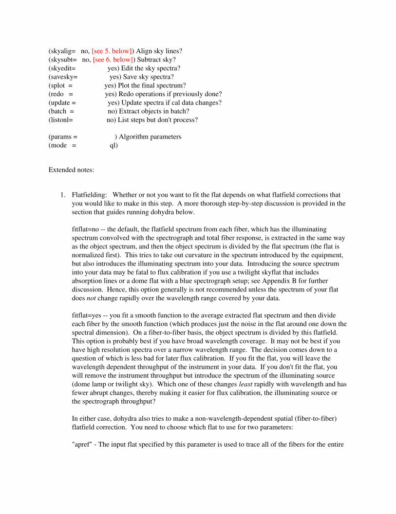
(skyalig=   no, [see 5. below]) Align sky lines?(skysubt=   no, [see 6. below]) Subtract sky?(skyedit=                  yes) Edit the sky spectra?(savesky=                  yes) Save sky spectra?(splot  =                  yes) Plot the final spectrum?(redo   =                  yes) Redo operations if previously done?(update =                  yes) Update spectra if cal data changes?(batch  =                   no) Extract objects in batch?(listonl=                   no) List steps but don't process?

(params =                     ) Algorithm parameters(mode   =                   ql)

Extended notes:

1. Flatfielding:   Whether or not you want to fit the flat depends on what flatfield corrections that you would like to make in this step.  A more thorough step­by­step discussion is provided in the section that guides running dohydra below. 

fitflat=no ­­ the default, the flatfield spectrum from each fiber, which has the illuminating spectrum convolved with the spectrograph and total fiber response, is extracted in the same way as the object spectrum, and then the object spectrum is divided by the flat spectrum (the flat is normalized first).  This tries to take out curvature in the spectrum introduced by the equipment, but also introduces the illuminating spectrum into your data.  Introducing the source spectrum into your data may be fatal to flux calibration if you use a twilight skyflat that includes absorption lines or a dome flat with a blue spectrograph setup; see Appendix B for further discussion.  Hence, this option generally is not recommended unless the spectrum of your flat does not change rapidly over the wavelength range covered by your data. 

fitflat=yes ­­ you fit a smooth function to the average extracted flat spectrum and then divide each fiber by the smooth function (which produces just the noise in the flat around one down thespectral dimension).  On a fiber­to­fiber basis, the object spectrum is divided by this flatfield. This option is probably best if you have broad wavelength coverage.  It may not be best if you have high resolution spectra over a narrow wavelength range.  The decision comes down to a question of which is less bad for later flux calibration.  If you fit the flat, you will leave the wavelength dependent throughput of the instrument in your data.  If you don't fit the flat, you will remove the instrument throughput but introduce the spectrum of the illuminating source (dome lamp or twilight sky).  Which one of these changes least rapidly with wavelength and hasfewer abrupt changes, thereby making it easier for flux calibration, the illuminating source or the spectrograph throughput?     

In either case, dohydra also tries to make a non­wavelength­dependent spatial (fiber­to­fiber) flatfield correction.  You need to choose which flat to use for two parameters:  

"apref" ­ The input flat specified by this parameter is used to trace all of the fibers for the entire 

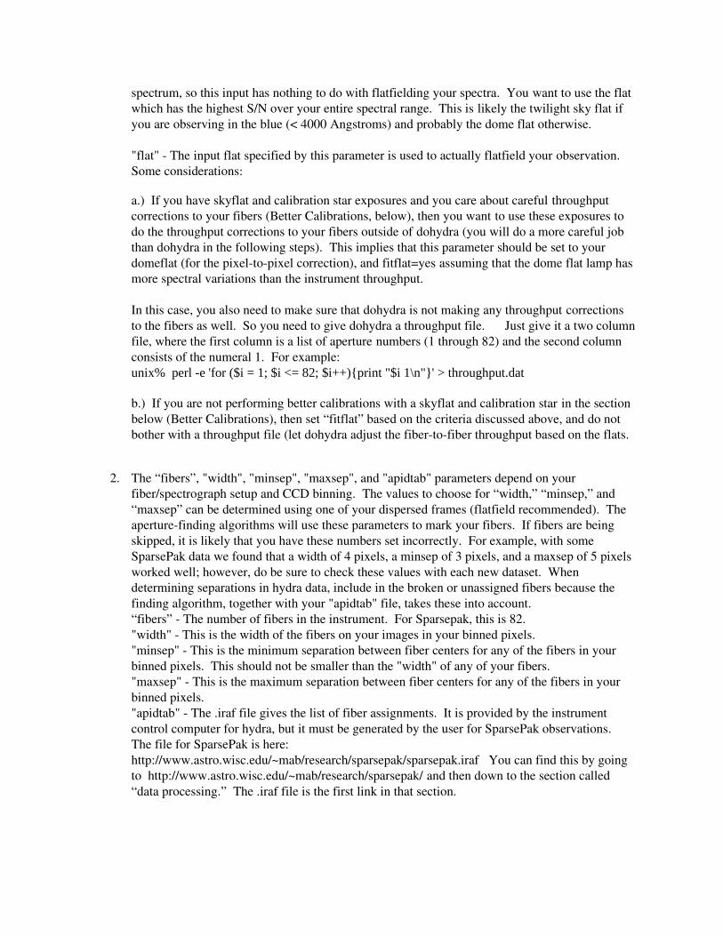
spectrum, so this input has nothing to do with flatfielding your spectra.  You want to use the flat which has the highest S/N over your entire spectral range.  This is likely the twilight sky flat if you are observing in the blue (< 4000 Angstroms) and probably the dome flat otherwise.  

"flat" ­ The input flat specified by this parameter is used to actually flatfield your observation.  Some considerations:

a.)  If you have skyflat and calibration star exposures and you care about careful throughput corrections to your fibers (Better Calibrations, below), then you want to use these exposures to do the throughput corrections to your fibers outside of dohydra (you will do a more careful job than dohydra in the following steps).  This implies that this parameter should be set to your domeflat (for the pixel­to­pixel correction), and fitflat=yes assuming that the dome flat lamp hasmore spectral variations than the instrument throughput.  

In this case, you also need to make sure that dohydra is not making any throughput corrections to the fibers as well.  So you need to give dohydra a throughput file.      Just give it a two columnfile, where the first column is a list of aperture numbers (1 through 82) and the second column consists of the numeral 1.  For example:  unix% perl -e 'for ($i = 1; $i <= 82; $i++){print "$i 1\n"}' > throughput.dat

b.)  If you are not performing better calibrations with a skyflat and calibration star in the section below (Better Calibrations), then set “fitflat” based on the criteria discussed above, and do not bother with a throughput file (let dohydra adjust the fiber­to­fiber throughput based on the flats. 

2. The “fibers”, "width", "minsep", "maxsep", and "apidtab" parameters depend on your fiber/spectrograph setup and CCD binning.  The values to choose for “width,” “minsep,” and “maxsep” can be determined using one of your dispersed frames (flatfield recommended).  The aperture­finding algorithms will use these parameters to mark your fibers.  If fibers are being skipped, it is likely that you have these numbers set incorrectly.  For example, with some SparsePak data we found that a width of 4 pixels, a minsep of 3 pixels, and a maxsep of 5 pixels worked well; however, do be sure to check these values with each new dataset.  When determining separations in hydra data, include in the broken or unassigned fibers because the finding algorithm, together with your "apidtab" file, takes these into account.“fibers” ­ The number of fibers in the instrument.  For Sparsepak, this is 82."width" ­ This is the width of the fibers on your images in your binned pixels. "minsep" ­ This is the minimum separation between fiber centers for any of the fibers in your binned pixels.  This should not be smaller than the "width" of any of your fibers. "maxsep" ­ This is the maximum separation between fiber centers for any of the fibers in your binned pixels. "apidtab" ­ The .iraf file gives the list of fiber assignments.  It is provided by the instrument control computer for hydra, but it must be generated by the user for SparsePak observations.  The file for SparsePak is here:  http://www.astro.wisc.edu/~mab/research/sparsepak/sparsepak.iraf   You can find this by going to  http://www.astro.wisc.edu/~mab/research/sparsepak/ and then down to the section called “data processing.”  The .iraf file is the first link in that section.  

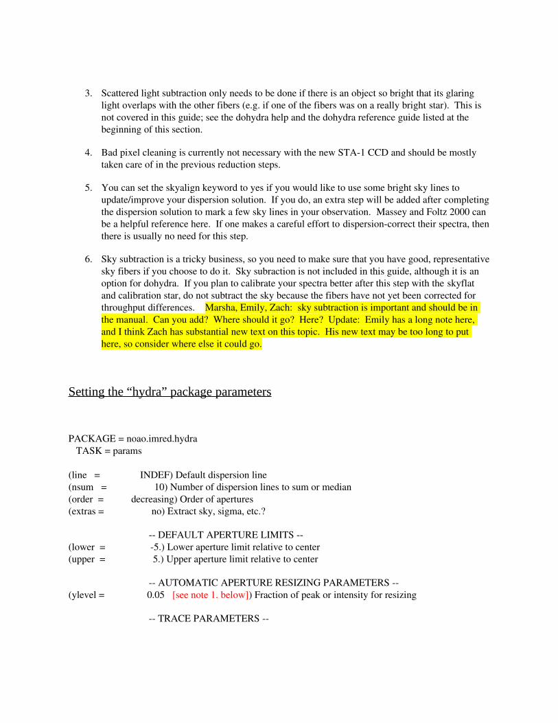
3. Scattered light subtraction only needs to be done if there is an object so bright that its glaring light overlaps with the other fibers (e.g. if one of the fibers was on a really bright star).  This is not covered in this guide; see the dohydra help and the dohydra reference guide listed at the beginning of this section.  

4. Bad pixel cleaning is currently not necessary with the new STA­1 CCD and should be mostly taken care of in the previous reduction steps.

5. You can set the skyalign keyword to yes if you would like to use some bright sky lines to update/improve your dispersion solution.  If you do, an extra step will be added after completingthe dispersion solution to mark a few sky lines in your observation.  Massey and Foltz 2000 can be a helpful reference here.  If one makes a careful effort to dispersion­correct their spectra, thenthere is usually no need for this step.

6. Sky subtraction is a tricky business, so you need to make sure that you have good, representativesky fibers if you choose to do it.  Sky subraction is not included in this guide, although it is an option for dohydra.  If you plan to calibrate your spectra better after this step with the skyflat and calibration star, do not subtract the sky because the fibers have not yet been corrected for throughput differences.    Marsha, Emily, Zach:  sky subtraction is important and should be in the manual.  Can you add?  Where should it go?  Here?  Update:  Emily has a long note here, and I think Zach has substantial new text on this topic.  His new text may be too long to put here, so consider where else it could go. 

Setting the “hydra” package parameters

PACKAGE = noao.imred.hydra   TASK = params    (line   =                INDEF) Default dispersion line(nsum   =                   10) Number of dispersion lines to sum or median(order  =           decreasing) Order of apertures(extras =                   no) Extract sky, sigma, etc.?

                                ­­ DEFAULT APERTURE LIMITS ­­(lower  =                  ­5.) Lower aperture limit relative to center(upper  =                   5.) Upper aperture limit relative to center

                                ­­ AUTOMATIC APERTURE RESIZING PARAMETERS ­­(ylevel =                 0.05   [see note 1. below]) Fraction of peak or intensity for resizing

                                ­­ TRACE PARAMETERS ­­

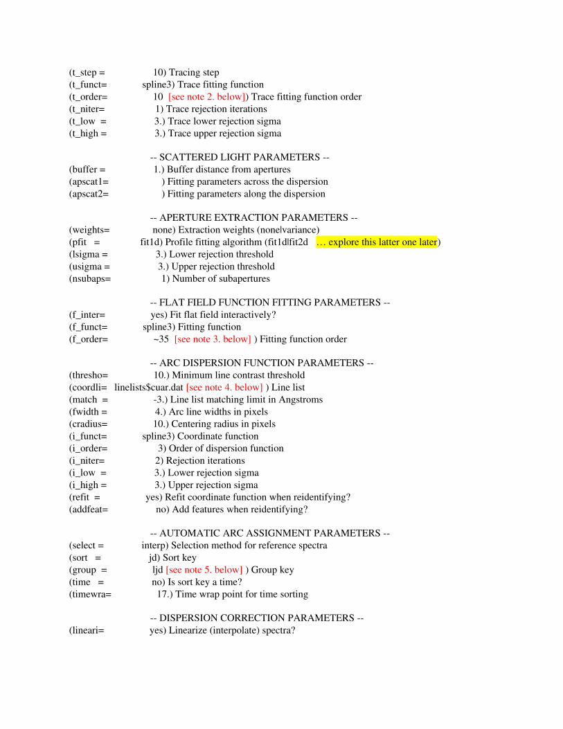
(t_step =                   10) Tracing step(t_funct=              spline3) Trace fitting function(t_order=                  10  [see note 2. below]) Trace fitting function order(t_niter=                    1) Trace rejection iterations(t_low  =                   3.) Trace lower rejection sigma(t_high =                   3.) Trace upper rejection sigma

                                ­­ SCATTERED LIGHT PARAMETERS ­­(buffer =                   1.) Buffer distance from apertures(apscat1=                     ) Fitting parameters across the dispersion(apscat2=                     ) Fitting parameters along the dispersion

                                ­­ APERTURE EXTRACTION PARAMETERS ­­(weights=                 none) Extraction weights (none|variance)(pfit   =                fit1d) Profile fitting algorithm (fit1d|fit2d   … explore this latter one later)(lsigma =                   3.) Lower rejection threshold(usigma =                   3.) Upper rejection threshold(nsubaps=                    1) Number of subapertures

                                ­­ FLAT FIELD FUNCTION FITTING PARAMETERS ­­(f_inter=                  yes) Fit flat field interactively?(f_funct=              spline3) Fitting function(f_order=                  ~35  [see note 3. below] ) Fitting function order

                                ­­ ARC DISPERSION FUNCTION PARAMETERS ­­(thresho=                  10.) Minimum line contrast threshold(coordli=   linelists$cuar.dat [see note 4. below] ) Line list(match  =                  ­3.) Line list matching limit in Angstroms(fwidth =                   4.) Arc line widths in pixels(cradius=                  10.) Centering radius in pixels(i_funct=              spline3) Coordinate function(i_order=                    3) Order of dispersion function(i_niter=                    2) Rejection iterations(i_low  =                   3.) Lower rejection sigma(i_high =                   3.) Upper rejection sigma(refit  =                  yes) Refit coordinate function when reidentifying?(addfeat=                   no) Add features when reidentifying?

                                ­­ AUTOMATIC ARC ASSIGNMENT PARAMETERS ­­(select =               interp) Selection method for reference spectra(sort   =                   jd) Sort key(group  =                  ljd [see note 5. below] ) Group key(time   =                   no) Is sort key a time?(timewra=                  17.) Time wrap point for time sorting

                                ­­ DISPERSION CORRECTION PARAMETERS ­­(lineari=                  yes) Linearize (interpolate) spectra?

(log    =                   no) Logarithmic wavelength scale?(flux   =                  yes) Conserve flux?

                                ­­ SKY SUBTRACTION PARAMETERS ­­(combine=              average) Type of combine operation(reject =            avsigclip) Sky rejection option(scale  =                 none) Sky scaling option(mode   =                   ql)

Notes:

1. The "ylevel" parameter is very important because this will determine the size of your extracted apertures.  The default value of 0.05 or 5% of the peak intensity from the center of each fiber seems to generally work well.

2. You should fit the trace of the fibers with the lowest­order function possible;  the dispersion of the spectrograph should be relatively smooth.  The recommended order seems to work well for any spectrograph settings that we have tried so far.  

3. "f_order" may need to be very high because the flat can have sharp curves in it caused by the spectrograph.  See 3. (the “fit the flat” section below)  for more information.

4. The default is to use the cuar.dat (Copper­Argon) line list.  If you used a different lamp for your data change this to the appropriate file name.  

5. Change the group parameter value if you are using data (e.g., calibrations from more than one night).  [See if this is explained elsewhere in the document – I know we were going to – and reference that if so.]

Run dohydra

The dohydra step is quite a beast, can be tedious, and is usually unforgiving if you make a mistake; sometimes you just have to start over; e.g., once you move on past a fiber, you cannot go back to it.  Take your time, check everything carefully, and record precisely what you do along the way, especially the information about the dispersion solution.  You will probably need to repeat this process afew times after the first time you try it.  You should make a separate directory for each configuration which holds the stacked object and calibration frames and run this task from that directory.

Only the four most commonly used and recommended steps are detailed below.

1.  Assign the fibers.

When you start dohydra, the first thing that will be asked is that you make sure that all fibers are numbered correctly (answer "yes" twice before getting to the window).  The fiber assignment is based on the file specified in the 'apidtab' parameter, which is part of the parameter set for the 

dohydra task.  If you are reducing hydra data you should have your ".iraf" file from your observation open for reference.   See Appendix D for more information regarding this step if you have hydra, as opposed to SparsePak, data.  

    

Note that only marked fibers with a 0 or 1 will actually be output by dohydra, *even if other fibers are marked*.  That is, fibers with a ­1, ­2, or 2 will not be output even if you mark them!  If you wantto extract any of these fibers, you need to modify the ".iraf" file so that these fibers are labeled with a0 or 1 in the second column.  While this implies that you do not need to delete any fibers that you don't want (unless they are denoted by a 0 or 1), this is not the whole story.  The dohydra task will still want to trace all marked fibers, even if they will not be output.  So, you should make sure that allof the good object (1) and sky (0) fibers are correctly denoted in the ".iraf" file, but also are the only ones marked in this step.   Otherwise, you will be prompted to trace garbage fibers, which can lead toerrors in dohydra.

Here are some commands that you will find most useful:

"wee" ­ zooms in on a window marked on the two opposite corners where you press "e" and "e"

“o" ­ renumbers all of the subsequent fibers according to how you number the current one

"d" ­ deletes a label for a fiber (so that the fiber is no extracted) without renumbering

"m" ­ mark a fiber with a number

"wl" ­ move left

"wr" ­ move right

"wa" ­ zooms back out to the default starting zoom

Once you are done with this step, press "q" to quit and move on to the next step.

2.  Trace the fiber positions along the chip.

The need for this step is described in Appendix C.  Next you will be prompted with "Fit traced positions for flat interactively (yes):".  You will want to do this for every fiber, so enter "YES" and hit enter.

Here are some commands that you will find most useful (the same zoom commands are available from the previous step):

":order" ­ change the number of spline functions for the fit (you may need to lower the order if you find that the program is fitting to noise or there are large excursions of the model away from the data).

"d" ­ delete points from the fit.

"u" ­ undelete points.

"f" ­ refit the trace.

    

Points that are marked with diamonds are 3­sigma outliers.  If you want to improve your RMS or are concerned that they are hurting the quality of your fit, you can delete them with "d" and then refit with "f".  You typically want your RMS to be below about 0.002, although you may not be able to dothis good if the end of the fiber is really noisy.  The default medium­order spline function (~10th­order) seems to do a pretty good job overall, but can sometimes get stuck in the noise or not fit the fiber trace well enough for you.  You should zoom in and check each fiber where it looks like there isa lot of bouncing around.  Type "q" to quit once you are done with the current fiber to move to the next.

3. Fit the flat (fitflat=yes; this is our default)

Note:  You are only prompted to complete this step when you choose fitflat=yes.  If you choose fitflat=no, the only thing that changes is that you do not fit a function to the average flat spectrum and divide it out.

You fit the average flatfield to take out the spectra shape so that you only make a pixel­to­pixel correction.  When fitting the flat, you might also notice an abrupt jump in the flat, which is likely an instrumental artifact caused by a drop in the blaze function of the grating (e.g., Wood's anomaly).  Because this can be a sharp drop in the flat, you might have to fit the flat with a high­order function.  You want to fit all of the curves very well here so that pixel­to­pixel variations are all that remain.  You may also have to delete the endpoints to get a good fit.  The rms is typically ~0.05% of the typical pixel values if the flat is well­fit and not too noisy.  See Appendix C for more details on fitting the flat and removing pixel­to­pixel variations with the flat field image using  dohydra.  

4.  Find the dispersion solution.

This can be the most difficult step.  You need figure out which pixel corresponds to which wavelength.  However, it is not as simple as finding the range of wavelengths because the dispersion of the spectrograph onto the CCD (Angstroms/pixel) changes as a function of position along the detector.  Therefore, you must fit a smooth function to this variable dispersion, (third order cubic spline function is used here and seems to generally work well).  You mark lines and fit a dispersion solution to one of your fibers (one near the center of the CCD) and then apply that dispersion solution to all of the fibers.

Here are some commands that you will find most useful (the same zoom commands are available from the previous steps):

"m" ­ mark a line with its wavelength

"d" ­ delete a marked line

"l" ­ mark the rest of the lines in the lookup table (from the line­marking step) OR show the non­linear component of the dispersion solution (after fitting)

"f" ­ fit the dispersion

"q" ­ quit to accept the dispersion solution

    

First, flip the x­axis with "wf" since the light is dispersed opposite to the numbered rows on the CCD (red­>blue, rows 1­>2000).  Now you will need to mark lines and identify them by entering their wavelength.  It is important to mark enough lines so that the algorithm can get close enough to be able to fill in all of the rest of the lines in the lookup table (linelists$cuar.dat, or whichever line list you used) correctly.  To get a reference plot to match to, go to the spectral atlas central at KPNO (http://www.noao.edu/kpno/ specatlas/ ), select the appropriate lamp, enter the expected wavelength range according to the spectrograph simulator, and tell it to output ~40 lines.  You will then use this reference to compare to your comparison lamp spectrum to mark the lines.  Figuring out which line iswhich can be difficult.  You want to look for patterns.  Note that "w+e+e" does not work to zoom in on a part of the spectrum when flipped!  You can get around this using the other "w" commands (type "w+?" to see them).  One way is to mark the left or right window edge and then shift left or right (w+l and w+r).

Mark each line and enter the appropriate wavelength (Angstroms).  You should mark ~10­20 lines     all across the spectrum.  Then typing "l" will tell dohydra to automatically try to interpolate in extra lines, which you may or may not want to do at this point (depending on how well you have marked lines and other factors such as the resolution of the spectrum; dohydra's automatic interpolation can fail in some instances and insert a number of points that you may want to delete anyway).  Type "f" to fit the spectrum and show the residuals.  Then type "l" to show the non­linear dispersion that you are trying to fit.  You can type "k,j,h" to examine other diagnostic plots of your fit.  Delete points andrefit with the same commands as were used on previous steps ("d","f") to improve the residuals.  To get back to the line marking, type "q" once, delete and remark lines, and iterate until the fit looks right.  In the non­linear component plot, which is the most important plot, the fit function and points should generally rise from 0 on the edges to a single maximum near the middle (the curve does not have to be symmetric).  We have found that you should be able to (and try to) get near an RMS of at least about an order of magnitude better than your spectral resolution.  The RMS, which is recorded in the logfile, is a lower limit to the uncertainty in your wavelength calibration.  When you are happy with the fit, type "q" from the line­marking plot to exit from this step for this aperture.

Then press enter ("NO") to reuse the dispersion solution for all of the fibers and avoid fitting the dispersion function interactively for each of the other fibers (you want to dispersion­correct consistently if you expect to compare or stack fibers later on; the dispersion should be similar enoughfor dohydra to handle anyway).  Finally press enter ("no") to avoid changing the wavelength coordinate assignments.  The final option is to view the spectrum with the splot task.  You can move from fiber to fiber with "(" and ")" and zoom in with the "w" options.

If you find that you have a difficult time marking the lines (it is not at all obvious which lines are which), then you can always copy over a previous "database" directory from a previous run of 

dohydra with the same spectrograph setup before you start dohydra.  This can save time if you have multiple configurations for the same spectrograph setup.  Note that the database directory is created by dohydra and where it stores some information about the steps that you had run (e.g., which wavelength corresponded to which pixels in the dispersion solution).  If you do this, you may need togo into those database files and change the filename designation (e.g., if you use configuration 1's database for configuration 2, you may need to change the 1's to 2's to get it to work).  Telling it to update the spectra if the cal data changes is particularly important if you do this.  If just copying over the database directory does not work (e.g., because you are in a different configuration where you areextracting different fibers), you can view the "idComp...ms" file in there.  It gives the pixel designation and matching wavelength for each marked line.  Finally, note that lower­resolution spectra can be more difficult to dispersion­correct because they do not look like the high resolution KPNO marked reference and because the KPNO line lists tend to have way more lines than you needor can resolve.

Better Calibrations

For the steps below, you will need to extract each of the skyflat and calibration star fibers with dohydra.  You should only continue with these steps if you followed the defaults for this guide by using the domeflat to make only pixel­to­pixel corrections (setting fitflat=yes).

For the calibration star, you just rerun dohydra on the calibration star exposure with the same method as you did for the stacked object frame except that you only extract (mark) the fiber with the calibration star on it (you can just count fibers on the exposure compared to the ".iraf" file to figure out what number to mark it as; the column number on the CCD can guide you too).  To only extract one fiber, you must delete all of the other fibers first and then mark that fiber as fiber 1 (or else dohydra maydie).  The fiber will be designated wrong, but it doesn't matter since you will be ignoring that fiber designation when referenced (see Notes 1. under calibrate task).  Also, note that since you only extract one fiber, make sure that the dispersion solution (starting and ending wavelengths, angstrom to pixel factor, and number of pixels is the same).

For the skyflat, you just rerun dohydra on the skyflat exposure with the same method as you did for the stacked object frame.

Finally, to help guarantee that you use the same dispersion solution on the calibration star spectrum and skyflat (very important), you can just make use of the "database" directory created when you ran dohydra on your object frames.

So, you now have a wavelength calibrated and extracted calibration star, skyflat, and object frame for a particular configuration.

Fiber-to-fiber and Spectrograph Throughout Corrections

Standard stars are observed typically with only a subset of the fibers, often just one fiber.  In order to get the most accurate flux calibration of fibers through which the standard was not observed, it is necessary to calculate and then apply a fiber­to­fiber throughput correction.  It is advantageous to use a twilight sky flat for this purpose because:  1) the rays are entering the telescope and instrument with the same distribution of angles as the night sky observations, which likely won't be true of dome flats; 2)it is difficult to get sufficient S/N in the blue with the existing dome flat lamps.  

First, run the sky flats through dohydra.  Many of the dohydra parameters are the same as those used above, but there are some very important differences:  

objects =               Skyflat  List of object spectra

(apref   = Domeflat or Skyflat [see notes below]) Aperture reference spectrum

(flat      = Domeflat [see notes below]) Flat field spectrum

(arcs1   = arc lamp closest in time to the twilight flats) List of arc spectra

(skysubt=   no) Subtract sky?  Definitely not, as you'll end up with nothing!

(fitflat   =  yes [see notes below]) Fit and ratio flat field spectrum?

Notes:

For red spectra it probably doesn't matter too much whether you use the dome flat or the sky flatfor apref.  However, for blue spectra, where the dome lamp is often quite weak, it is much preferred to use the sky flat as the apref.  Does dohydra let you use the same image for both objects and apref?  Check this, and if it has a problem, tell the reader to make a copy of the sky flat with a different name to use as the apref.  

It probably makes sense to turn on flat­fielding here only if you're going to fit the flat and  correct for pixel­to­pixel variations.  In that case, you definitely want to use the dome flat, as thesky flat has too many absorption lines to fit adequately.  

Next, take the ratio of the extracted spectrum from each fiber and divide it by the spectrum froma reference fiber.  The reference fiber must be one in which the standard star was observed every time you pointed to a standard during the night.  If you placed the standard on multiple fibers each time you observed it, pick the fiber which covers the region of the CCD with the fewest defects (bad pixels/rows/columns) and/or covers the most important region of your science targets.  Note that the 

output of this next step, ratios of sky flat spectra, should contain the value 1 (to within arithmetic precision) for all pixels in the reference fiber.                                            PACKAGE = onedspec   TASK = sarith

input1  =      Skyflat.ms.fits  List of input spectraop      =                    /  Operationinput2  = Skyflat.ms.fits[*,#]     [See 1. below]  List of input spectra or constantsoutput  = Skyflat_ratio.ms.fits List of output spectra(w1     =                INDEF) Starting wavelength(w2     =                INDEF) Ending wavelength(apertur=                     ) List of input apertures or columns/lines(bands  =                     ) List of input bands or lines/bands(beams  =                     ) List of input beams or echelle orders(apmodul=                    0) Input aperture modulus (0=none)

(reverse=                   no) Reverse order of operands in binary operation?(ignorea=                  yes) Ignore second operand aperture numbers?

(format =            multispec) Output spectral format(renumbe=                   no) Renumber output apertures?(offset =                    0) Output aperture number offset(clobber=                   no) Modify existing output images?(merge  =                   no) Merge with existing output images?(rebin  =                   no) Rebin to exact wavelength region?(errval =                   0.) Arithmetic error replacement value(verbose=                   no) Print operations?(mode   =                   ql)

Notes:

1. The character # represents the row in the extracted spectrum that has the calibration star.  You must figure out this spectrum number and enter it here; e.g., consult the heading of splot.  Note that counting is started from 1, so the APNUM keyword is the same number.

Since the ratios will be noisy, fit them with a mathematical function, and then later use this function as the fiber­to­fiber throughput correction.                                         PACKAGE = onedspec   TASK = sfit

input   =     Skyflat_ratio.ms  Input imagesoutput  =      Skyflat_corr.ms  Output images(lines  =                    *) Image lines to be fit(bands  =                    1) Image bands to be fit(type   =                  fit) Type of output(replace=                   no) Replace rejected points by fit?

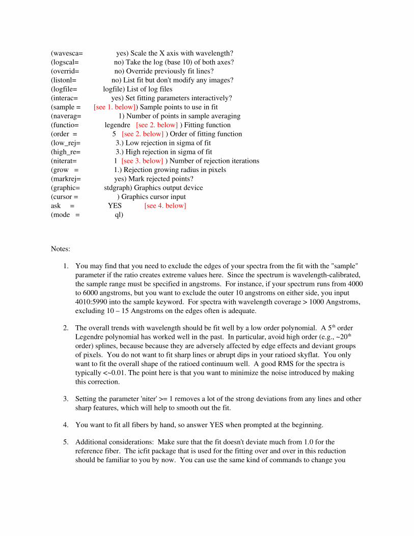
(wavesca=                  yes) Scale the X axis with wavelength?(logscal=                   no) Take the log (base 10) of both axes?(overrid=                   no) Override previously fit lines?(listonl=                   no) List fit but don't modify any images?(logfile=              logfile) List of log files(interac=                  yes) Set fitting parameters interactively?(sample =       [see 1. below]) Sample points to use in fit(naverag=                    1) Number of points in sample averaging(functio=              legendre   [see 2. below] ) Fitting function(order  =                   5   [see 2. below] ) Order of fitting function(low_rej=                   3.) Low rejection in sigma of fit(high_re=                   3.) High rejection in sigma of fit(niterat=                    1  [see 3. below] ) Number of rejection iterations(grow   =                   1.) Rejection growing radius in pixels(markrej=                  yes) Mark rejected points?(graphic=             stdgraph) Graphics output device(cursor =                     ) Graphics cursor inputask     =                  YES            [see 4. below]                            (mode   =                   ql)

Notes:

1. You may find that you need to exclude the edges of your spectra from the fit with the "sample" parameter if the ratio creates extreme values here.  Since the spectrum is wavelength­calibrated, the sample range must be specified in angstroms.  For instance, if your spectrum runs from 4000to 6000 angstroms, but you want to exclude the outer 10 angstroms on either side, you input 4010:5990 into the sample keyword.  For spectra with wavelength coverage > 1000 Angstroms, excluding 10 – 15 Angstroms on the edges often is adequate.  

2. The overall trends with wavelength should be fit well by a low order polynomial.  A 5th order Legendre polynomial has worked well in the past.  In particular, avoid high order (e.g., ~20th order) splines, because because they are adversely affected by edge effects and deviant groups of pixels.  You do not want to fit sharp lines or abrupt dips in your ratioed skyflat.  You only want to fit the overall shape of the ratioed continuum well.  A good RMS for the spectra is typically <~0.01. The point here is that you want to minimize the noise introduced by making this correction.  

3. Setting the parameter 'niter' >= 1 removes a lot of the strong deviations from any lines and other sharp features, which will help to smooth out the fit. 

4. You want to fit all fibers by hand, so answer YES when prompted at the beginning.

5. Additional considerations:  Make sure that the fit doesn't deviate much from 1.0 for the reference fiber.  The icfit package that is used for the fitting over and over in this reduction should be familiar to you by now.  You can use the same kind of commands to change you 

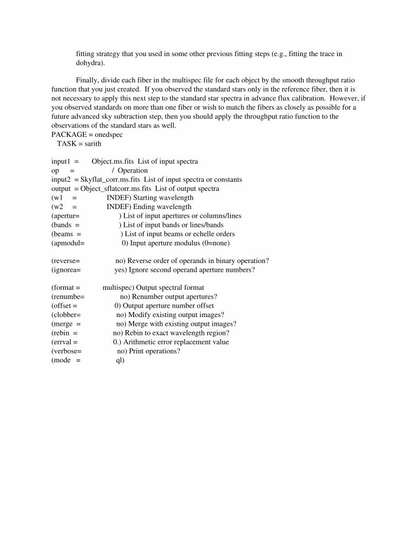
fitting strategy that you used in some other previous fitting steps (e.g., fitting the trace in dohydra).

Finally, divide each fiber in the multispec file for each object by the smooth throughput ratio function that you just created.  If you observed the standard stars only in the reference fiber, then it is not necessary to apply this next step to the standard star spectra in advance flux calibration.  However, ifyou observed standards on more than one fiber or wish to match the fibers as closely as possible for a future advanced sky subtraction step, then you should apply the throughput ratio function to the observations of the standard stars as well.                                              PACKAGE = onedspec   TASK = sarith

input1  =       Object.ms.fits  List of input spectraop      =                    /  Operationinput2  = Skyflat_corr.ms.fits  List of input spectra or constantsoutput  = Object_sflatcorr.ms.fits  List of output spectra(w1     =                INDEF) Starting wavelength(w2     =                INDEF) Ending wavelength(apertur=                     ) List of input apertures or columns/lines(bands  =                     ) List of input bands or lines/bands(beams  =                     ) List of input beams or echelle orders(apmodul=                    0) Input aperture modulus (0=none)

(reverse=                   no) Reverse order of operands in binary operation?(ignorea=                  yes) Ignore second operand aperture numbers?

(format =            multispec) Output spectral format(renumbe=                   no) Renumber output apertures?(offset =                    0) Output aperture number offset(clobber=                   no) Modify existing output images?(merge  =                   no) Merge with existing output images?(rebin  =                   no) Rebin to exact wavelength region?(errval =                   0.) Arithmetic error replacement value(verbose=                   no) Print operations?(mode   =                   ql)

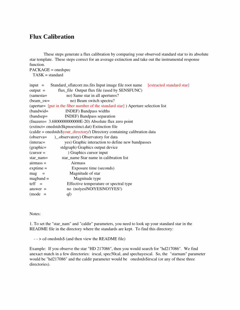
Flux Calibration

These steps generate a flux calibration by comparing your observed standard star to its absolute star template.  These steps correct for an average extinction and take out the instrumental response function.                                            PACKAGE = onedspec   TASK = standard

input   =      Standard_sflatcorr.ms.fits Input image file root name     [extracted standard star]output  =            flux_file  Output flux file (used by SENSFUNC)(samesta=                  no) Same star in all apertures?(beam_sw=                   no) Beam switch spectra?(apertur=  [put in the fiber number of the standard star] ) Aperture selection list(bandwid=                INDEF) Bandpass widths(bandsep=                INDEF) Bandpass separation(fnuzero=  3.6800000000000E­20) Absolute flux zero point(extinct= onedstds$kpnoextinct.dat) Extinction file(caldir = onedstds$your_directory/) Directory containing calibration data(observa=       )_.observatory) Observatory for data(interac=                  yes) Graphic interaction to define new bandpasses(graphic=             stdgraph) Graphics output device(cursor =                     ) Graphics cursor inputstar_nam=             star_name Star name in calibration listairmass =                       Airmassexptime =                       Exposure time (seconds)mag     =                       Magnitude of starmagband =                       Magnitude typeteff    =                       Effective temperature or spectral typeanswer  =                   no  (no|yes|NO|YES|NO!|YES!)(mode   =                   ql)

Notes:

1. To set the "star_nam" and "caldir" parameters, you need to look up your standard star in the README file in the directory where the standards are kept.  To find this directory:

    ­ ­ > cd onedstds$ (and then view the README file)

Example:  If you observe the star "HD 217086", then you would search for "hd217086".  We find anexact match in a few directories:  irscal, spec50cal, and spechayescal.  So, the  "starnam" parameter would be "hd217086" and the caldir parameter would be   onedstds$irscal (or any of these three directories).   

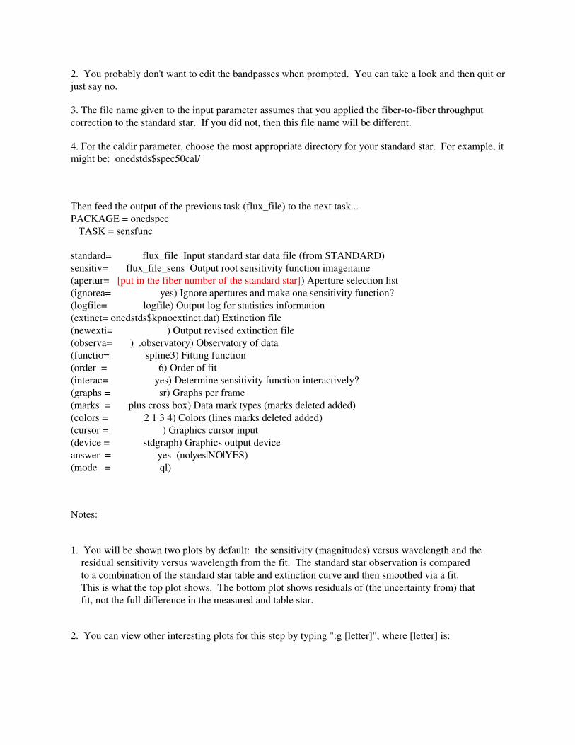
2.  You probably don't want to edit the bandpasses when prompted.  You can take a look and then quit orjust say no.

3. The file name given to the input parameter assumes that you applied the fiber­to­fiber throughput correction to the standard star.  If you did not, then this file name will be different.  

4. For the caldir parameter, choose the most appropriate directory for your standard star.  For example, itmight be:  onedstds$spec50cal/

Then feed the output of the previous task (flux_file) to the next task...                                         PACKAGE = onedspec   TASK = sensfunc

standard=            flux_file  Input standard star data file (from STANDARD)sensitiv=       flux_file_sens  Output root sensitivity function imagename(apertur=   [put in the fiber number of the standard star]) Aperture selection list(ignorea=                   yes) Ignore apertures and make one sensitivity function?(logfile=              logfile) Output log for statistics information(extinct= onedstds$kpnoextinct.dat) Extinction file(newexti=                     ) Output revised extinction file(observa=       )_.observatory) Observatory of data(functio=              spline3) Fitting function(order  =                    6) Order of fit(interac=                  yes) Determine sensitivity function interactively?(graphs =                   sr) Graphs per frame(marks  =       plus cross box) Data mark types (marks deleted added)(colors =              2 1 3 4) Colors (lines marks deleted added)(cursor =                     ) Graphics cursor input(device =             stdgraph) Graphics output deviceanswer  =                  yes  (no|yes|NO|YES)(mode   =                   ql)

Notes:

1.  You will be shown two plots by default:  the sensitivity (magnitudes) versus wavelength and the    residual sensitivity versus wavelength from the fit.  The standard star observation is compared    to a combination of the standard star table and extinction curve and then smoothed via a fit.    This is what the top plot shows.  The bottom plot shows residuals of (the uncertainty from) that    fit, not the full difference in the measured and table star.

2.  You can view other interesting plots for this step by typing ":g [letter]", where [letter] is:

    e ­ Extinction (and revised extinction) vs wavelength

    i ­ Flux calibrated image vs wavelength

    l ­ Log of flux calibrated image vs wavelength

    r ­ Residual sensitivity vs wavelength

    s ­ Sensitivity vs wavelength

    ":g sr" is the default and is most important to look at

    There are a couple other options that are only interesting when you use multiple standard stars at various airmasses.

The bottom line is that you probably won't change anything here unless you get a bad fit.

Finally, you apply your sensitivity corrections to the spectrum...                                      PACKAGE = onedspec   TASK = calibrate

input   = Object_sflatcorr.ms.fits  Input spectra to calibrateoutput  = Object_calibrated.ms.fits  Output calibrated spectra(extinct=                  yes) Apply extinction correction?(flux   =                  yes) Apply flux calibration?(extinct= onedstds$kpnoextinct.dat) Extinction file(observa=       )_.observatory) Observatory of observation(ignorea=                  yes) Ignore aperture numbers in flux calibration?(sensiti= flux_file_sens.[fiber#]) Image root name for sensitivity spectra[fiber#] should be 0001 if you marked it in the dohydra step as directed above(fnu    =                   no) Create spectra having units of FNU?airmass =                       Airmassexptime =                       Exposure time (seconds)(mode   =                   ql)

Notes:

1. Since this guide suggests that you just extract out the calibration star in the dohydra step (for simplicity), you need to set the "ignorea" parameter to "yes" in this step.  Then, the task will apply the same correction to all of your extracted fibers.

2. If you receive a warning that there are a certain number of pixels outside of the calibration limits, this is probably because the sensitivity function does not extend completely to the edge of your spectrum.  This could be because the absolute standard does not cover the full 

wavelength range that you observed or simply because the sensfunc task did not provide a sensitivity function out to the edge of your observation (the calibration is completed in  discretized steps and those steps do not always go to the edge of your range).  In any case, since you should not rely on the observations at the edge of any spectrum for a variety of reasons, excluding only a handful of pixels around the edges of a spectrum is nothing to sweat over.  Note that the number of excluded pixels is the total number of excluded pixels over all fibers.

3. Since this absolute calibration method uses only one standard star and an average extinction, it is difficult to quantify the uncertainty in the absolute calibration.  Using multiple stars over multiple airmasses would give a better handle on this.  For instance, one can take a ratio of the sensitivity functions (count to erg conversion as a function of wavelength; the "flux_file_sens.0001" file above). In any case, note that any subsequent flux uncertainties that you calculate are only relative uncertainties, which represent a lower limit to the absolute uncertainty.  Note also that no scattered light correction is made for the standard star in the dohydra step, which means that  the absolute flux will be different depending on how much stray light is scattered into the fibers away.  Furthermore, other factors can affect the absolute calibration from one setup to another:  changing weather, poor guiding, etc. (because the fiber does not catch all of the light from a star).  If you compare multiple configurations taken at different times (even of the same night), you may need to use the ratio of the sensitivity functions to provide you single non­wavelength­dependent offset factor with which to scale the observations.  The typical uncertainties in the absolute calibration are frequently non­negligible and a function of wavelength.  In any case, you should not expect to absolutely calibrate your spectra to better than ~10%.

4. Finally, the units are in erg/cm^2/s/A.

Advanced Sky Subtraction

The standard methods for sky subtraction do a reasonable job but often do not reduce the bright sky line residuals to the Poisson limit.  In fact, in some cases there are large excursions in the object spectra due to insufficient sky subtraction.   Part of the reason for this is discussed in one of the SparsePak papers (Bershady et al., 2005, ApJS, 156, 311):  "Because the optical transfer function (OTF) varies over spectrograph field angles, the width and shape of spectrally unresolved lines changes along the (pseudo­) slit." The spectral lines in different fibers across the CCD will appear in different positions, and unresolved lines will have slightly different widths in different fibers (so that, when stacking, the lines get unnaturally broadened).

Applying the fiber­to­fiber relative throughput corrections to all fibers before sky subtraction, orfor a secondary follow­up sky subtraction, should improve the result.  Methods to improve the sky subtraction will be described here in the future.

ConclusionCONGRATULATIONS! You have an extracted and calibrated spectrum for each fiber in your

observation.

At this point, you will want to come up with a way to identify each fiber with a position on the sky.  This involves matching the coordinates in the ".hydra" configuration file with the fiber numbers that you marked as good in the ".iraf" file.  The last number in parentheses in the ".iraf"file corresponds to the number in the first column of the ".hydra" file.  You can also use the header of the spectrum file toget some of the fiber information.  For instance, one of the authors of this guide wrote an IDL program that does this automatically:  "get_fiber_coord.pro"

Good Luck!

Appendix A: Very brief introduction to PyRAF and IRAF

IRAF is the core software system we are using.  It is very powerful, but it suffers from a rather old user interface.  While a brief discussion of IRAF, including how to get it started, is presented below, this guide assumes general familiarity with IRAF; it describes in detail only those procedures used in thereduction of SparsePak data.  The Space Telescope Science Institute (STScI) provides a python wrapper to IRAF called PyRAF.  Much, though by no means all, of the discussion in this guide applies equally toIRAF and PyRAF.  The main advantage of PyRAF is the ability to write code in a modern language, python, that can call IRAF tasks.  However, PyRAF also improves some of the IRAF user interface issues, though anachronisms like keystrokes as the only option to interactively control graphics windowspersist.  See the references at the end of this section for introductions to IRAF and PyRAF.  

In this manual, commands preceded by "unix%" are general terminal (unix shell) commands.  Your terminal prompt likely will not be the exact string “unix%”; this is just a placeholder for whatever it is on your system.  The terminal commands can be run from within PyRAF/IRAF by prepending themwith an exclamation mark (the so­called “bang” symbol)4.  However, it is generally cleaner, especially for new users, to run all of the unix shell commands in a dedicated terminal window that is separate from PyRAF/IRAF.  You should launch PyRAF in a separate terminal window, and IRAF will have to be launched from its own special terminal as well.  It is dangerous to have PyRAF and IRAF, or any twoIRAF­based sessions for that matter, running at the same time, so close one before starting the other.  Asyou use different terminals for unix shell commands and PyRAF/IRAF, make sure that each is in the correct directory at every step.  PyRAF and IRAF commands are preceded by their own prompts, as explained below.   

PyRAF can be started from any regular xterm, as long as you're in the directory containing your login.cl file (often your home directory): 

unix% pyraf

This will load PyRAF and place you in the interactive PyRAF shell, from which you edit parameters andlaunch PyRAF tasks, with the following prompt:

­ ­ >  

Much of the new data reduction and analysis code that uses tasks from IRAF is written in PyRAF.  In fact, new software is being written in PyRAF to improve SparsePak reductions.  For all of these reasons we strongly suggest that users employ PyRAF rather than IRAF unless it is absolutely 

4

  You can also define unix shell commands as external tasks within your login.cl file, a file that gives IRAF some guidance when it starts, if you want to type them without the bang.  See the lines in the login.cl that start with the word 'task' and end with the string ' “$foreign” .'  Note that shell commands with switches or arguments may not work right from within PyRAF/IRAF, even if you have defined them as external; in that case use the bang to escape the command directly to the shell. 

necessary to revert to the original IRAF command interface.   Once you start PyRAF (or IRAF) in the directory with your login.cl file you can use the 'cd' command to change directories to whichever you want.  

For the few times when it is necessary to run IRAF by itself, you must first check your login.cl file in your home directory.  If 'xterm' is selected, then you must run IRAF from within an xterm, but note that you will lose much of the graphics functionality.  To access the full graphics capability, you must have xgterm installed on the system, have xgterm selected within the login.cl file, and start IRAF from within an xgterm window.  The standard implementation is launched from the unix command line via: 

unix% cl

The command 'cl' is short for “command line,” in reference to the IRAF command line interface.  The IRAF interactive prompt will appear as: 

cl> 

An “extended command line with more functionality can be launched with: 

unix% ecl

The “extended cl” IRAF prompt will appear as: 

ecl>

Finally, IRAF v. 2.16 (the latest as of this writing) includes virtual observatory features, and its command prompt is:

vocl>

[Note to authors:  is there a difference between typing 'cl', 'ecl', and 'vocl' in v. 2.16?  ]

PyRAF/IRAF tasks are organized into packages, which can be nested into sub­packages, sub­sub­packages, etc.  Some packages are loaded automatically every time you start up PyRAF/IRAF.   These default packages are listed in your login.cl, typically fairly close to the end of the file.  You can load packages interactively by typing the package name at the PyRAF/IRAF prompt.  Once a package isloaded you do not have to re­load it for the duration of that PyRAF/IRAF session.  However, if you starta new session you must make sure that all of the packages you need are loaded.  The full sequence of packages is listed at the top of the parameter listing for each task used in this guide.  You can find the same listing for any task at the top of its help page.  For example, the package listing for the ccdproc task is noao.imred.ccdred .  The “noao” high level package should be one of those in your login.cl, hence is loaded automatically, and you should not need to type it.  However, the others may not be in your login.cl, in which case load them by typing on the PyRAF/IRAF command line: 

 ­ ­ > imred

 ­ ­ > ccdred

Interacting with PyRAF/IRAF:

1. Type "?" in any IRAF graphics window to see available commands.  Type "help [taskname]" to get more information about that task.  

2. To edit parameter files in PyRAF/IRAF, you type "epar [taskname]”.  This will bring up a text editor when launched from within IRAF, but a gui will appear if you're using PyRAF.  Once in the parameter editor, you can make a parameter blank by hitting the spacebar.  To save the parameters wtihin PyRAF, simply hit the appropriate button in the gui.  To save the parameters when you're using IRAF, invoke something similar to  VI syntax:  ' :q ' to quit, ' :wq ' to write the parameters and then quit.  After you quit the parameter editor within IRAF in this manner, type the task name and hit return at the IRAF prompt to execute the task.  

3. When IRAF prompts you for a response, an uppercase "NO" or "YES" automatically repeats command for the set that you are working on while a lowercase "no" or "yes" only accepts the response for the current subtask.   

4. To reset a parameter file to its default values, use "unlearn [task]" within IRAF.  There is an “unlearn” button on the epar GUI in PyRAF.   

5. Mac specific notes (aka, “McNotes”): 

You can use 'function delete' in place of backspace in IRAF (e.g., when editing a parameter file using epar; at least on a Mac).  

The command for editing a line in epar mode is 'control u l' (at least on a Mac).  

Graphics: 

1. The "display" task in PyRAF/IRAF may not automatically display the entirety of a large image (check the stdimage setting in your login.cl, and edit there or on the command line as necessary)and does not easily  allow you to access the full range of values in the image.  For exploring the 2­D image it is better to load the image directly into ds9 (via the 'file'   'open' menu selection). →However, any PyRAF/IRAF task which requires user interaction with the image will only work if the image is loaded from within PyRAF/IRAF.  

2. IRAF's "implot" can be useful for plotting along lines and columns (for quickly visualizing data).  You can also get some of this functionality from within the general purpose and highly useful task 'imexam' (use 'c' and 'l' keystrokes to get column and line plots, respectively, from around the image).  

3. To save an encapsulated postscript plot, which you should do frequently to have a record of your graphics window work, execute the following from within the graphics window     ' :.snap eps ' Then you must rename the resulting output file to something appropriate.

Helpful references:

1. http://iraf.noao.edu/iraf/ftp/pub/beguide.ps.Z  This is supposed to be a beginner's guide, but it currently (14 AUG 2012) has link rot.  

2. http://iraf.noao.edu/iraf/ftp/iraf/docs/ccduser3.ps.Z  IRAF CCD users' guide. 

3. http://iraf.noao.edu/iraf/ftp/iraf/docs/ccdguide.ps.Z  Guide to the IRAF ccdred package.  Old, but still probably useful.  

4. http://iraf.noao.edu/iraf/ftp/iraf/docs/clean.ps.Z  Cleaning bad pixels and cosmic rays in IRAF. 

5. http://iraf.noao.edu/iraf/ftp/iraf/docs/dofibers.ps.Z  Discussion of the dofibers package in IRAF, of which dohydra is a variant.  

6. http://iraf.noao.edu/iraf/ftp/iraf/docs/dohydra.ps.Z  IRAF's dohydra task, which is the heart of the extraction of the fiber spectra in this guide.  

7. http://iraf.noao.edu/iraf/ftp/iraf/docs/fits_userguide.ps.Z  Discussion of how IRAF handles FITS images.  This is a useful overview, especially for multi­spec or multi­extension fits files.  This isa bit old, so be on the lookout for any obsolescence.  Hard­core fits I/O is more likely to be donewith PyFITS (http://www.stsci.edu/institute/software_hardware/pyfits) these days.  

8. The "Handbook of CCD Astronomy" by Steve Howell is a good introduction to using CCDs for imaging or spectroscopy. 

9. http://www.wiyn.org/Instruments/wiynsta1vst2ka.html (information for the CCD)

10. http://www.astro.wisc.edu/~mab/research/sparsepak/ (Matt Bershday's SparsePak webpages)

11. http://www.astro.wisc.edu/wiyn/wiyn.html (general UW­specific information for WIYN)

12. http://www.noao.edu/kpno/specatlas/ (comparison lamp information)

13. http://www.astro.wisc.edu/~crawford/Spectrograph/spect.html (bench spectrograph simulator). This link is very useful for determining your spectrograph setup.  Knowing the resolution, the central wavelength, and wavelength range, you can go through the gratings and orders and check which setting is most efficient at which camera­collimator angles by plotting this angle versus the efficiency.  It is a bit out of date, but can still be very useful to give one a sense of what configurations are available and best to use for you observational requirements.

14. http://www.noao.edu/cgi­bin/kpno/wiyn/hydrasetup.pl (for estimating S/N with Hydra)

15. http://www.noao.edu/wiyn/ (general WIYN webpage, which includes links for observing and instrument information)

Appendix B: Overview of different types of images

Here are brief descriptions of the types of exposures that you could take during your observing run, or will find in an existing data set, and explanations as to the purpose of these exposures with regardto the reduction process:

Overscan

The overscan is a region outside of the illuminated part of the detector.  This is used to monitor and correct for time variation in the (unwanted) signal produced by the electronics.  In some detectors, such as near­infrared detectors, these are physical pixels which are shielded from light.  Typically in CCDs these are virtual pixels.   After reading out the real CCD pixels, the system continues to read out virtual pixels to record the bias level and read noise of the amplifiers (like sucking on a straw after all of the liquid is gone). These virtual pixels are placed in the overscan region.  The overscan subtraction is accomplished by averaging the pixels along each row of a column to create an average column from the overscan region.  Then, one fits a smooth function to this average column and subtracts this smooth function from each column of the CCD.  For the WIYN spectrograph CCD, this makes a big difference because the amplifiers add a large pedestal to the number of counts in each pixel (e.g., out of 16500 counts, 16000 of them could be from the amplifier).

Zeros

Zero (also called “bias”) exposures are taken to remove 2­D structure in the CCD imprinted from the manufacturing of the CCD and the control electronics.  These frames are zero­second exposures that immediately read out the initial electron levels throughout the CCD.  These are the easiest exposure to take.  Since the shutter does not open and the exposure time is effectively zero seconds, the entire spectrograph setup does not matter here.

We recommend taking at least 50 zero exposures per night at a convenient time (afternoon, dinner).  Thebias pattern can change somewhat with time.  Radical changes in the zero frames may indicate detector problems.  

Darks

These exposures are taken to remove thermally generated electrons in the CCD during the exposure.  Only long exposures (>~ a few minutes) have appreciable dark current (short exposures have not had a long enough time to accumulate appreciable dark current), and even then it is usually not large

in modern CCDs.  The dark frames are exposed with the shutter closed for the same length of time as theobject frames that you are dark­correcting.  Note that the dark current is frequently not linear with time, so scaling the dark frames to correct other length exposures is risky but sometimes done.  Dark exposures also may help subtract some hot pixels.

The spectrograph setup also does not matter for dark exposures.  Take as many as you can, at least 10 – 20 per night, while you are sleeping or at another convenient time.  

Flats

There are two types of flats: domeflats and (twilight) skyflats.  Domeflats are easier because youcan take them at any time under controlled conditions.  However, they do not work as well as skyflats for some crucial applications.  You use flatfields to make sensitivity corrections for the system of instruments you are using:  pixel­to­pixel variations in the CCD, fiber­to­fiber throughput differences of the fibers, and vignetting from the telescope and the spectrograph.  Discussion of flats specific to the Hydra instrument is presented in Appendix D.            

Domeflats:

Domeflats can be used to correct for pixel­to­pixel sensitivity variations in the CCD if you first fit and remove the spectrum to arrive at a spectrally flat image containing only the pixel­to­pixel variations.  This is typically done because twilight sky flats contain deep and complex absorption lines which are difficult, if not impossible to fit adequately.  Dome flats may have low signal in the blue (< 4000 Angstroms) due to low instrument throughput and a red lamp, so you may have to take more exposures to get sufficient S/N in the blue part of the spectrum5.   You can  make the dome lamp bright enough so that you get a lot of signal in a relatively short exposure, but don't go too short (typically 1 to a few seconds is too short) or you might introduce erroneous features due to the finite time it takes for the instrument shutter to open and close.  To maximize you S/N, your domeflats can be resonably close to the non­linearity limit of the CCD without exceeding it; in particular, beware of over­exposing in the red.  You should take many domeflats to provide sufficient S/N from blue to red.         

Domeflats produce spectra at a different focus and temperature than the sky, which can have various effects on the calibrations.  These and the other limitations above are why we use skyflats...        

5

In principle you could abstain from fitting the flat in the spectral direction.  This would impart both the spectrum of the illuminating source (either the sky or a lamp in the dome) and the spectral response of the instrument to the data.  Again, in principle, these effects could be removed with the standard star.  However, inpractice this is not usually a good idea because the twilight sky has a complex spectrum and if the flat lamp is red (any thermal lamp without filters) its emission will fall rapidly in the blue.  Both of these effects will be hard to remove with the observation of the standard star.  Hence, you need dome flats, and at least for blue spectra, you should fit and remove the spectral variations from these flats.  

Skyflats:

Skyflats make superior corrections to domeflats in all cases except for the CCD pixel­to­pixel corrections discussed above.  There are various reasons why skyflats tend to produce a better flatfield:  the Sun illuminates the clear sky over a small angular field more evenly than any dome lamp on the screen both in the spatial and spectral dimensions; there is enough scattered blue light in the sky for veryblue observations; and the sky projection (focus) is effectively at infinity.            

Skyflats will always make more accurate corrections for fiber­to­fiber throughput differences of the fibers themselves and vignetting from the telescope and the spectrograph.  These statements imply that if you care about comparing the relative or absolute flux in fibers to high precision (e.g., for comparing faint objects in different fibers), you really need take skyflats.  The default for this guide is touse skyflats so that we to make throughput corrections as accurately as possible in the reductions below. 

Skyflats should be always taken in the same setup as your object exposures.  Skyflats must be taken starting either shortly after sunset and/or shortly before sunrise.  Since the sky changes color during this time, you want to take all skyflats that you will be stacking together as close together in time as possible.  "Shortly after" or "shortly before" above usually means ~10­30 minutes, so this is a very short window.  This limits hydra to two configurations per night if you take them in the configurations that you observe your objects, as recommended for the reasons above, because resetting and setting up the fibers usually takes much too long (~30 minutes).  Each exposure should take about a minute or less.

To summarize this lengthy discussion, we find that we usually incorporate domeflats only to make CCD pixel­to­pixel sensitivity corrections (and sometimes to trace apertures in the dohydra reduction step) and use skyflats to correct for fiber­to­fiber throughput differences of the fibers themselves and vignetting from the telescope and the spectrograph plus to trace apertures for blue spectra.  However, calibration in the spectral direction can only be done accurately through the use of a standard star...   

Standard Star

The only way to to calibrate your fluxes, is to make use of one or more standard star(s).  Make sure that you take standard star exposures through one of the fibers that you used to observe your object(s).  Each exposure should take about less than a minute.  Otherwise, you are probably wasting your time with too                    faint of stars.  A list of standards can be retrieved in IRAF's "onedstds$" directory.  See the flux calibration step near the bottom for more information.  Take at least two standardstars through the night so that you can check the accuracy of your calibrations.  In particular, you shouldtake a standard star calibration if the weather appears to change so that you can check your calibrations. You should put the stars on the same fiber so that all other system effects cancel in the ratio comparison.

Note:  When observing point sources like standard stars or other stars in the object frames, this guide currently makes the assumption that essentially all of the light from the star is collected by the fiber in question.  For SparsePak (5" fibers) and Hydra (3" blue fibers; 2" red fibers), this is usually a safe assumption because the stellar seeing disk is almost always smaller than the size of any of the fibersunder typical seeing conditions at WIYN.  However, this assumption breaks down if the seeing disk of 

the star becomes greater than or about equal to the size of the fibers or if one uses smaller fibers, as is the case on the next generation of fiber instruments (HexPak, GradPak).  One should always make sure that each fiber collects all of the light from each star or be prepared to make a correction for the amount of light lost.  Therefore, using the smallest fibers ~1 arcsec to observe point sources is not adviseable unless your pointing and seeing is excellent.

These points are moot when observing diffuse flux.  In the case of observing diffuse flux in the smallest fibers, the skyflat can be used to provide the scaling factor from a larger fiber that the standard star is observed on to the smaller fibers.  This method is OK even if the different fibers have a different spectrally­dependent response because the calibrations in this guide are made as a function of wavelength.

Comparison Lamps

A few of these need to be taken right before or after your observation (in the same fiber configuration when using hydra) so that you can figure out which pixel corresponds to which wavelength in the spectral direction.  You usually use a ~1 minute or less exposure time.  However, you may need to vary the exposure time to bring out brighter or fainter lines for your wavelength calibration.

Objects

These are the observations of your targets.  In order to remove cosmic rays effectively and easily, you should always take a minimum of 3 exposures, regardless of you exposure time (this is actually a general statement for all exposures above).  This implies that it is better to take 3 20­minute exposures than to take 1 60­minute exposure.  The read time is fairly short (~1 minute) and read noise is small with the current CCD, so more exposures does not add significantly more read noise (you are probably never going to be read noise limited with the fiber spectrographs).

Appendix C: Layout and Fiber Numbering Scheme of the IFU Bundles

HexPak and GradPak have a few broken, or otherwise very low throughput fibers. The original numbering scheme assigned numbers to those dead fibers and counted them as part of the numeric sequence. However, the task dohydra will number only fibers that it can find, namely the ones which are illuminated. The original numbering scheme would create a mismatch between the fiber numbering on the schematics and the numbering of spectral traces created by dohyra. For this reason the numbering on the schematics was recast to count only the fibers with enough throughput to appear as illuminated, which brings the schematics in line with the numbering assigned by dohydra. The HexPak and GradPak schematics presented below adhere to this new numbering scheme, in which only the illuminated fibers are counted.

SparsePak

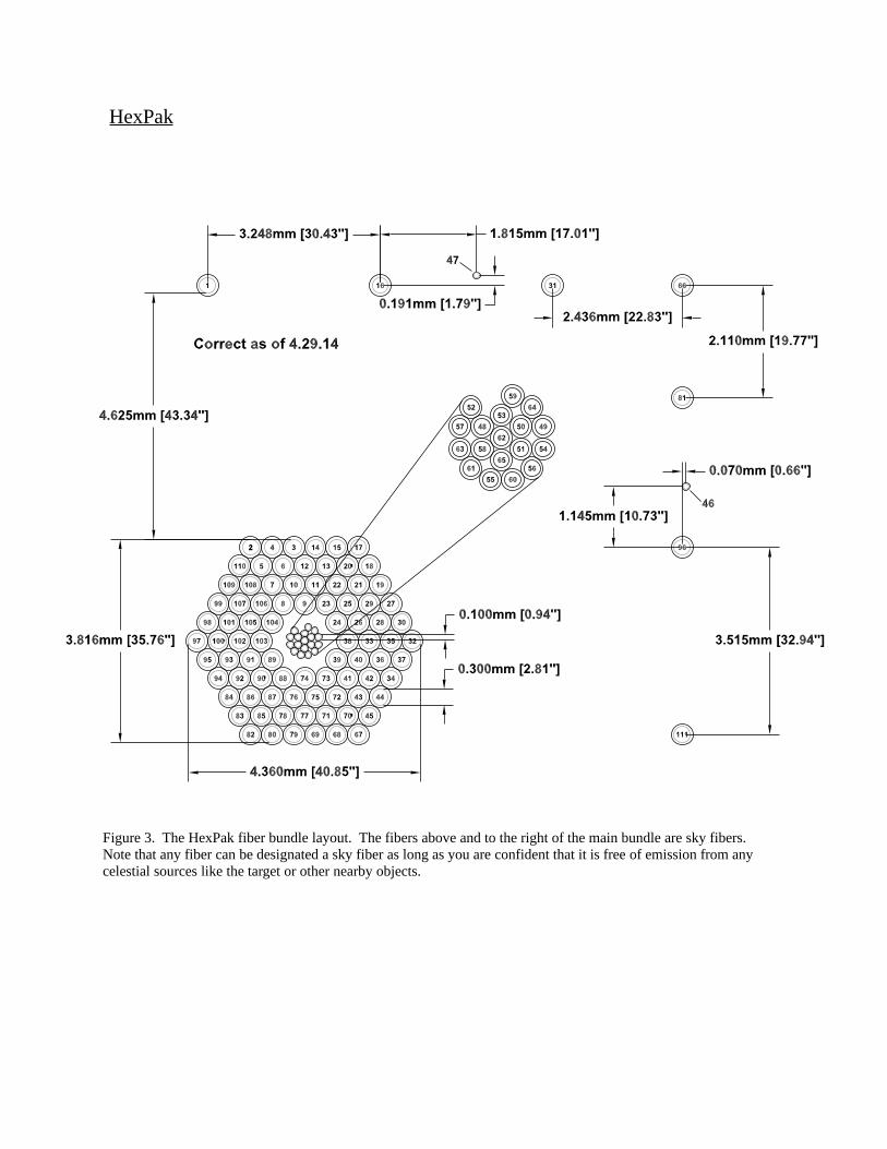
HexPak

Figure 3. The HexPak fiber bundle layout. The fibers above and to the right of the main bundle are sky fibers. Note that any fiber can be designated a sky fiber as long as you are confident that it is free of emission from any celestial sources like the target or other nearby objects.

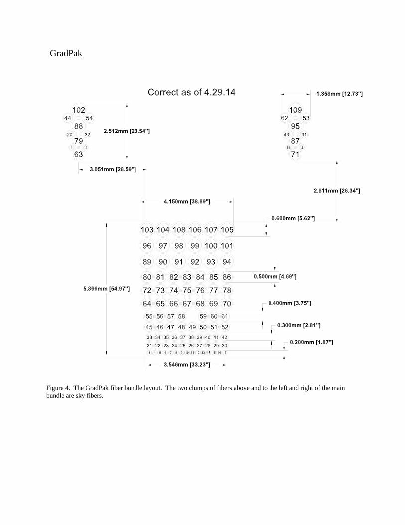
GradPak

Figure 4. The GradPak fiber bundle layout. The two clumps of fibers above and to the left and right of the main bundle are sky fibers.

Appendix D: Bench Spectrograph Characteristics

The characteristics of the Bench Spectrograph and its CCD that are the most important for data reduction are summarized here.  Consult the WIYN website for more details and the latest information.

Two CCD characteristics can be set by the user, gain and binning.  Several criteria should be considered in choosing the binning and gain: 

Binning.  

o The most fundamental consideration is sampling in both the spatial, and especially the spectral dimensions.  This will depend mainly on the fiber sizes, which affect both the spatial and, usually, the spectral binning, but also on the focus across the 2­D image produced by the spectrograph. To achieve Nyquist sampling make sure that there are at least 2 pixels per resolution element in both dimensions.  For example, with the 600@10.1 grating we typically use the following binning (be sure to check for your own grating and setup!):  4 (spatial) X 3 (spectral) with SparsePak and 2 (spatial) X 1 (spectral) with HexPak.

o Readout time depends strongly on binning.  In general, unless you need to finely samplethe spatial profile or spectral lines for some particular high precision work that requires it, bin as much as you can while still adequately sampling the profiles.  The readout timefor 1x1 binning at high gain is prohibitively long.  

o You may wish to choose a smaller binning factor, less coarse binning, if you are worried about accumulating too many counts in a pixel and hitting numeric saturation, such as extremely bright sources.  For many applications this is not a consideration except for flats, and in most cases it is probably unwise to let calibration observations, over which you have significant control, determine your observing parameters.  

Gain. 

o Higher gains (larger values when measuring ADU / electron; smaller when quoting values as the inverse, e­ / ADU) give lower read noise values.  If your sky noise will be above the read noise, or you do not care about the low S/N portions of your spectrum, then this aspect will not concern you; otherwise, it may be the dominant consideration. 

o Higher gains will get you to the numeric saturation limit of 256K ADU with fewer electrons / photons.  If you have bright objects you may wish a lower gain so that you don’t hit numeric saturation as quickly, in which case the higher read noise will not be an issue.  This is not a concern with fainter objects, though do be careful with bright standard stars and flat fields.  We have gotten into some trouble pushing the flats too hard to build signal in the blue and numerically saturating the red end of the spectrum 

(this is done occasionally by design in twilight flats, but if you do this with dome flats you may end up with no useful dome flats).  

o Higher gains increase the readout time.  This consideration drives one to as low a value for gain that can be tolerated for read noise in order to maximize observing efficiency.  For our data the tradeoff is primarily between read noise and readout time.  We tend to opt for better read noise since our program target exposures tend to be 20 – 30 minutes, making the additional readout penalty less of an issue.  However, this was a closer call with HexPak, since the small fibers requires finer binning, which in turn greatly increases the readout time.  Observers with shorter exposure times, especially using HexPak’s small fibers, should carefully weigh the tradeoff between read noise and readout time.  

The maximum values one should allow per pixel depend on several considerations.  The fundamental limit is the saturation of the pixel, the point at which the potential well which constitutes the pixel can no longer hold any more electrons.  Any additional photons are not recorded, and heavily over­saturated pixels can affect nearby pixels as well.  Before that point, however, the pixel’s response to light becomes increasingly non­linear.  A careful observer should stay safely below the non­linearity threshold.  The Hydra manual lists the 1% non­linearity threshold as ~80,000 e­ and the saturation limit as ~ 100,000 e­.  With the adopted gain, these values can be expressed as ADU, which is the value you actually see in the data.  For example, with a gain of 0.2 e­ / ADU, the physical non­linearity and saturation thresholds become 400,000 and 500,000 ADU, respectively.   However, this is not the full story, and in this particular example you will hit a major problem at data values well below the physical limits.  

The additional consideration is the limit of the value which can be represented by the CCD’s analog­to­digital converter.  In the case of our device, this numeric saturation level is 256,000 ADU.  In the case of the previous example with a gain of 0.2 e­ / ADU, you will hit numeric saturation well beforephysical saturation.  Alternately, if you use a gain of 0.8 e­ / ADU you will hit the physical non­linearityand saturation limits well before the numeric saturation level.  Beware of these considerations, or else they may bite you in the tuschie and lead to unusable data.  

Appendix E: More detailed discussions

Some of the justifications for reductions steps and choices, while quite important, are too long for the main text and break the flow.  These justifications and explanations are given here.  

The Use of Laplacian Edge Detection to Remove Cosmic Rays in SparsePak Data

Laplacian edge detection has been found to work quite well on many 2­D images of the sky and traditional long­slit spectra.    See van Dokkum's implementation (http://www.astro.yale.edu/dokkum/lacosmic/) plus a local how­to (http://www.astro.wisc.edu/~cigan/reducing/lacos/lacos.html).  However, it does not appear to work well on Sparsepak data.  We think that the image of the fiber, which forms the line function, is too sharp:  the Laplacian algorithm thinks that sky lines are cosmic rays.  If the algorithm parameters are adjusted so that the sky lines are not removed, then too many real cosmic rays also are not flagged.  Further investigations may uncover a sweet spot for the application of this method to SparsePak data.  In particular, Ben Brown suggested using a wavelet approach to de­tune the method to the specific shape ofa fiber, while flagging all other sharp­edged objects.  However, until further work can be done, the use of Laplacian edge detectors for cosmic ray removal in Sparsepak data is strongly deprecated at this time.

If you wish to try Laplacian edge detection, be very careful.  It’s easy to look quickly at the nrejmask image and see what looks to be only real cosmic rays and seemingly bad pixels among the rejected values.  However, some of these may be emission lines.  Blink the data frame against the nrejmask image to make sure that none of the rejected values consistently correspond to real features.  Since no one has yet managed to get lacosmic to avoid rejecting real features in Pak data, be sure to check carefully if you think you’ve figured out how to do it.     

Setting Parameter 'statsec' in Task 'imcombine'

Fiber data present a challenge to choosing a region over which to calculate image statistics (the 'statsec' parameter) for scaling, assigning weights, etc.  This arises from the presence of dark regions between each of the illuminated fibers, which may adversely impact some statistics.  There should be noproblem if one uses the average, since relative weights and scales will still behave properly in the presence of dark regions (though zero point adjustments may be dubious).  However, the average is more sensitive to outliers than the median or mode.  Unfortunately, the median and mode may be unstable in this situation.   The best way to see this is to imagine an idealized case of alternating purely dark regions (value 0) and uniformly bright regions (for example, assume a value of 1 for the sake of this discussion).  If there is one more dark pixel than bright pixel, the median will be 0; however, if thereis one more bright pixel, then the median suddenly switches to 1.  Similarly for the mode, there will be two distinct peaks of the histogram and so this statistic can flip between the two extremes with only slight differences in the input image.  In practice this may not be such a drastic problem for Sparsepak if 

the number of “bright” pixels is routinely significantly larger than the number of “dark” pixels.  However, this should be investigated before blithely using a large fraction of the image for the statsec (as is typically done for imaging data or bias/dark frames) when employing median or mode.  A prudent compromise is to use a restricted statsec centered on only a single fiber when calculating median or mode statistics for scaling or weights.    

Combining all of the Twilight Flats, Even when the Spectra are very Different

Do the twilight spectra need to be very similar to each other in order to combine them?  No, as long as you use a weighted average and don't include saturated values.  The simple case, where no values are rejected, is considered first.

Each input spectrum is Fλ,_,k, where k is the number of the observation in the sequence of twilight flats.  The throughput is Tλ,j,_, where j is the fiber number (throughput is assumed to be the same in a given fiber for all of the exposures in the sequence, which is the reason this value is not indexed by k).  The observed spectrum of the kth exposure in fiber number j is Oλ,j,k = Tλ,j,_ X  Fλ,_,k.  We'll have a single weight for each exposure, Wk.  The weighted average spectrum for fiber j is (each of the sums is over all of the exposures, indexed by k):

Aλ,j = Σ (Oλ,j,k  X  Wk ) /  Σ Wk  =  Σ  (Tλ,j,_ X  Fλ,_,k.  X  Wk ) /  Σ Wk  =  Tλ,j,  Σ (Fλ,_,k.  X  Wk )  /  Σ Wk .  

Each individual spectrum, Fλ,_,k , can be quite different as long as each fiber is illuminated by the same input spectrum and has the same weight for a given twilight flat observation, k. 

Next pick a particular fiber as the reference fiber, j = r, and divide this spectrum into each of theother fibers:  

Aλ,j /  Aλ,j=r  =  Tλ,j,_ / Tλ,j=r,  because the factors Σ (Fλ,_,k.  X  wk )  /  Σ wk in the numerator and denominator cancel (they do not depend on the fiber number, j).    Hence, the ratio of the weighted averages for two fibers provides the ratio of the throughputs for these fibers.    

However, there is an important consideration, and a subtle potential problem, when rejection of discrepant values, whether through thresholding or clipping, is allowed.  Consider a mask function Mλ,j,k 

which is 1 if a given value is to be included in the weighted average and 0 if it is to be excluded.  This mask depends on the position in the spectrum (wavelength), the fiber (j), and the exposure number in thesequence (k).  The dependence on j arises because different fibers have different throughput functions (measuring these is the whole point of the exercise) so that the flux at a given wavelength may be above the threshold in one fiber but below it in the other.  The dependence on k arises because the twilight sky spectrum is constantly changing.   Now the weighted average spectrum for fiber j becomes: 

Aλ,j = Tλ,j,  Σ (Fλ,_,k.  X  Wk  X Mλ,j,k)  /  Σ Wk .  The ratio with respect to the reference fiber becomes: 

Aλ,j /  Aλ,j=r  = ( Tλ,j,_ / Tλ,j=r ) X  (Σ (Fλ,_,k.  X  Wk  X Mλ,j,k) / Σ (Fλ,_,k.  X  Wk  X Mλ,j=r,k) )

Note that the only way in which the second term, after the ratio of throughputs, cancels for a given pair of fibers, j and r, is if Mλ,j,k = Mλ,j=r,k  for all exposures k at each wavelength.  In general the culling of values is conducted independently for each pixel when the 2­D images are combined.  Hence, Mλ,j,k Mλ,j=r,k  .  If the mask functions for two fibers are relatively close the measured ratio may be a reasonable approximation to the ratio of the throughputs.  However, in regions of the spectrum where the values are close to the threshold value, a modest difference in throughput may cause several values to be masked in one fiber while the corresponding values are not masked in the other fiber.  Essentially this changes the effective input spectrum, which violates the fundamental assumption upon which this method is based.  This effect can give the wrong Tλ,j,_ / Tλ,j=r  in regions of the spectrum where the sky flatis close to the threshold value.

The correct way to deal with this problem is to ensure that Mλ,j,k = Mλ,j=r,k  for all exposures k at each wavelength.  This will have to be done pairwise between every fiber j and the reference fiber j = r.  The rejmask pixel list images provided by imcombine encode all of the information about rejected pixels.  The difficulty with employing the 2­D rejmask directly is that the different fibers j and r have differently shaped traces on the 2­D images.  The regions of the 2­D masks corresponding to each fiber cannot be overlaid with each other without a geometric transformation to make them coincident with each other.  This could be challenging to make work correctly, including the fact that it may be difficult to ensure that rejected values do not slip through.  A simpler approach, and probably adequate, would beto create master masks in 1­D.    

It will be easier to create and use a set of 1­D master masks by first reversing the meaning of themask values, Mλ,j,k, such that 0 corresponds to a value that should be kept and 1 means that the value should be rejected.  Construct the 1­D masks by first running imcombine on the twilight flat images in the standard way, followed by tracing, extracting, and wavelength calibrating the combined twilight flats.  Then apply the same traces and wavelength calibration to each plane in the rejmask image stack, such that there is a 1­D mask spectrum for every wavelength of each fiber in each of the sky flat exposures.  If any of the 2­D rejmask pixels which contribute to a 1­D wavelength pixel have a mask value = 1 (remember, this now means the pixel is rejected), then the 1­D pixel will have a value  1, which means that pixel is considered rejected.    

Next extract 1-D spectra from each of the individual twilight flat images that were used to make the combined 2-D flat in the previous step. Do not let dohydra create a separate trace and wavelength calibration for each of these extractions. Rather, use the trace and wavelength calibration that dohydra determined when extracting the spectra from the combined 2-D flat above, the same as used to extract the mask spectra. The reason for this is so that all spectra, as well as the corresponding mask spectra, were extracted and wavelength calibrated in exactly the same way. In summary, the reason to combine the 2-D twilight images is to create a rejection mask for each of the individual twilight images; the only reason for extracting and wavelength calibrating the combined image first is to have a common set of extraction apertures and wavelength calibrations for these operations on the individual images and rejection masks.

At this point there is a multispec file, containing the 1-D spectra for every fiber, for each twilight flat exposure. For each of these files there is a corresponding multispec file containing 1-D spectral masks for each fiber. If a mask value is 0 then the value of the twilight flat at the correspondingwavelength is considered good and should be included in the weighted average. If the mask value is

other than 0 (should be  1, in fact) then the twilight flat value is bad and should be excluded in the weighted average.  

The weighted average of the extracted 1­D twilight sky spectra cannot be done in bulk, with IRAF automatically taking care of every fiber in the multispec files.  The reason is that the mask spectra must be used in a pairwise manner to make sure the same values are masked in each of the pair of spectra. For fiber j and reference fiber r in twilight flat observation k, add the corresponding 1­D mask spectra:  

Mλ,j & r,k  = Mλ,j,k  +  Mλ,r,k  

Use Mλ,j & r,k  for each observation k when making the weighted average of all 1­D spectra for fiber j, Aλ,j, and use the same mask spectrum when doing the weighted average of the reference fiber spectra r, Aλ,r .  Then move on to the next fiber in the sequence, j.  Even though the reference fiber is thesame, the combined mask spectrum Mλ,j & r,k  will have to be generated anew because in general Mλ,j,k   Mλ,j,k .  Hence, the reference fiber spectrum will have to be re­generated each time using the new mask Mλ,j & r,k .

Now take the ratio of the weighted average spectra as before,

Aλ,j /  Aλ,r for j   = Tλ,j / Tλ,r .  Note that the reference spectrum, Aλ,r for j , is specific for fiber j, as explained previously.  This reference spectrum will be different for the next fiber j.  Continue as described in the main part of the manual by fitting a function to Tλ,j / Tλ,r  and then using this fit to adjust the wavelength dependent throughputs of each fiber to that of the reference spectrum.  

NOTES for further checking:  

Do threshold rejected values get included in the mask?

How to Adjust Task 'dohydra' so that it Does not Crash when Using Data from More than One Night

If  some of your exposures are from different nights, then dohydra will crash at the very end of the process without properly finishing its task with the following error: 

[Skyflat] No reference spectrum found Input [Skyflat] ljd = ...number1... : Ref [Cuar_1] ljd = ...number2... No arc reference assigned for Skyflat 

where Skyflat and Cuar_1 refer to the actual values for these parameters you supply to dohydra and ...number1... and ...number2... are the LJDs from the image headers of the input calibration exposures. 

            The dohydra task checks the "LJD" header keywords for consistency (to make sure that you use skyflats and arcs from the same night).  However, if this is not the case IRAF crashes rather than providea warning.   If you choose to use a calibration from a different night, then you need to change the "group" keyword in the "params" input parameter file in the package noao.imred.hydra, described in the dohydra section of the main part of this manual.  Change the value of this 'group' parameter from "LJD" to the name of another image header keyword from your run that has the same value in all of your input exposures, such as "OBSERVAT" or "TELESCOP".  Simply changing the LJD in the header of the input file does not work as dohydra seems to check multiple keywords. Basically, this appears to be a bug workaround where you have a fudge the value to get dohydra to run correctly. 

Tracing the Fiber Positions in Task 'dohydra'

The tracing of the fibers refers to how they are extracted along the columns of the CCD.  This is important if the fibers are not perfectly parallel to the columns of the CCD, but close.  You can check this subtlety by displaying the flat in ds9 and putting your cursor over the center of a fiber, noting its column number, and then checking the column number of the center of this fiber on the other end of the chip.  You will find that the fiber is not perfectly aligned with the columns of the chip.  This is why you have to trace the fiber position as it changes columns along the dispersion.  This depends on the fiber, but the center usually shifts by a few pixels from end to end.  The default for this guide is to fit a moderately high­order cubic spline function to compensate for these column shifts.  You can try other functions but the spline seems to do a pretty good job.  You want to fit the overall shape of the shifts well, but you want to avoid fitting to the noise.  You will do this for each fiber individually since each dispersed fiber that you are extracting is curved along the CCD a little differently (and you may need to delete outlying points to make for a better fit), so this can be tedious if you use a noisy flat.

Pixel-to-pixel Corrections in the Task 'dohydra '

The process by which dohydra makes flatfield corrections is:

Using the trace for each fiber that you fit from the domeflat (or skyflat in case you are extracted extremely blue spectra <~4000A where the dome lamp shines very faintly), dohydra averages (for each fiber independently) the pixels along each row (across the fiber in the spatial direction)for the domeflat and for the corresponding object spectrum.

Dohydra then normalizes each domeflat fiber independently by its spectral average.  This is the intermediate domeflat that is output by dohydra.  It provides a single row for each fiber, where the values are normalized to be around 1.  Since the spectral signature is present, the difference from end to end can be >~10%.

Using the function that you fit to the flatfield formed from the average spectrum across all fibers, it divides each fiber by that function to mostly take out the lamp spectrum and the wavelength dependent throughput.  So, all that is left is the pixel­to­pixel variations (and noise) 

~ 1 for each pixel along the each spatially­averaged fiber. Dohydra does not provide this spectrally­divided domeflat.

Finally, dohydra divides each object fiber by its corresponding processed flatfield fiber to take out pixel­to­pixel variations.  By dividing each fiber in the flat field image by a fit to the average flat, you will not remove all spectral variations.  The deviations in the shape of each flatfield compared to the average will remain.  As long as these deviations are small in amplitude and smooth, they can be removed by flux calibration.   During this process, dohydra can compare each fiber and calculate a single fiber­to­fiber throughput correction factor from the flat, which you prevent it from doing by giving dohydra a throughput file (all values 1.0).

To make pixel­to­pixel corrections, dohydra sums the pixels in the spatial direction for each fiber of the flatfield and then divides by the flatfield instead of dividing by the 2­D flatfield, as is done inimaging.  This does not appear to be mathematically equivalent at first glance, but it is because one has no spatial resolution within each fiber (the pixels in the spatial direction do not actually provide any spatial information).  While each pixel along the fiber in the spatial direction records different levels of counts because of the throughput differences (PSF) of the fiber in different parts of the fiber, that light has already been averaged out (integrated by the fiber), neglecting all spatial differences on the sky smaller than the fiber.  That is, because one has no spatial resolution from within the fiber, the flux term from the illuminating source per pixel can always be taken out of the sum of the pixels because it is a constant (an average).  This is why it doesn't matter whether you sum/average then divide (what dohydradoes) or divide then sum/average.  However, it does matter, for instance, in long­slit spectroscopy, where you have retained spatial information along the long­slit. 

Appendix F: Some notes on the Hydra instrument

Hydra is another fiber instrument on WIYN.  Rather than an IFU with fixed fibers, it has movable fibers which can be positioned around the field of view.  This is particularly useful for clusters of objects, such as star clusters or galaxy clusters.  Hydra has more fibers than Sparsepak.  These fibers feed the same Bench Spectrograph.  The reduction steps for Hydra are similar to those for Sparsepak, but there are important differences.  Brief discussions of these differences may appear in the main text, but longer explanations are contained in this appendix.  

Dome Flats with Hydra

There are two domeflat fiber configurations (where the fibers are positioned differently on the focal plane) that you can use:       

bluecircle or redcircle (same effects for either the blue or red fibers) ­­ In this configuration, the fibers are positioned at equal distances from the center of the focal plane.  This means that the dome lamp will essentially illuminate the fibers evenly.  In the object frames, then you could correct for the fiber­to­fiber throughput differences of the fibers themselves and the vignetting from the spectrograph.  Because this method corrects for the most effects, it is the most effectivedomeflat method to use.  However, there is one main limitation: since the fibers are at different locations on the focal plane than in the object frames, you will not correct for vignetting from the telescope optics.

The fibers are in the same position as when you observe your object field ­­ In this configuration, the fibers are not equally illuminated by the dome lamp. This implies that you cannot sort out if the differences in fiber brightness are from the fiber­to­fiber throughput differences, from the fibers themselves multiplied by the vignetting of the spectrograph, or are from the fact that the dome lamp has not illuminated the fibers equally.  However, you could correct for the vignetting from the telescope optics because the fibers are in the same positions on the sky as your object frames.

We currently do not have a measure of the magnitude of each of these corrections, so it is hard to say which method is superior except to mention that all fibers are out in bluecircle or redcircle, so thiscan be used regardless of the configuration.  If  in doubt, we recommend that you just use bluecircle or redcircle as it can correct  for the most throughput differences.  The circle configuration domeflat can beused  for any fiber setup since all of the (non­broken) fibers are extended and equally illuminated.

            

Running dohydra

The fiber assignment file, denoted by .iraf should be generated by the telescope.  You need to include the name of this file in the 'apidtab' parameter that is included in the parameter set for the dohydra task.  

You need to make sure that all fibers that have a 0 or 1 in the ".iraf" file are marked correctly.  Note that broken and unassigned fibers remain parked at the perifery of the plate, but are still active, so light from objects or the sky can still enter them.  This can make them look like good fibers when they really are    not.  Also note that areas labeled "gap" in your ".iraf" file will never have light and can be very useful reference points for assigning fibers.