Hyperparameter estimation for uncertainty

quantification in mesoscale carbon dioxide inversions

By LIN WU1,2*, MARC BOCQUET2,3 , FREDERIC CHEVALLIER1, THOMAS LAUVAUX4

and KENNETH DAVIS4, 1Laboratoire des Sciences du Climat et de l’Environnement,

CEA-CNRS-UVSQ, IPSL, Gif-sur-Yvette, France; 2Universite Paris-Est, CEREA, Joint Laboratory

Ecole des Ponts ParisTech � EDF R&D, Marne la Vallee, France; 3INRIA, Paris-Rocquencourt Research Center,

France; 4Department of Meteorology, Pennsylvania State University, State College, PA, USA

(Manuscript received 19 March 2013; in final form 10 October 2013)

ABSTRACT

Uncertainty quantification is critical in the inversion of CO2 surface fluxes from atmospheric concentration

measurements. Here, we estimate the main hyperparameters of the error covariance matrices for a priori fluxes

and CO2 concentrations, that is, the variances and the correlation lengths, using real, continuous hourly CO2

concentration data in the context of the Ring 2 experiment of the North American Carbon Program Mid

Continent Intensive. Several criteria, namely maximum likelihood (ML), general cross-validation (GCV) and

x2 test are compared for the first time under a realistic setting in a mesoscale CO2 inversion. It is shown that the

optimal hyperparameters under the ML criterion assure perfect x2 consistency of the inverted fluxes. Inversions

using the ML error variances estimates rather than the prescribed default values are less weighted by the

observations, because the default values underestimate the model-data mismatch error, which is assumed to be

dominated by the atmospheric transport error. As for the spatial correlation length in prior flux errors, the

Ring 2 network is sparse for GCV, and this method fails to reach an optimum. In contrast, the ML estimate

(e.g. an optimum of 20 km for the first week of June 2007) does not support long spatial correlations that are

usually assumed in the default values.

Keywords: hyperparameter estimation, uncertainty quantification, mesoscale carbon dioxide inversions

1. Introduction

The atmosphere integrates the CO2 source�sink fluxes at

all space and time scales to form a spatiotemporal CO2

field. Consequently, the atmospheric CO2 mole fraction

measurements convey signals from CO2 fluxes, which can

be described by an observation equation:

l ¼ Hxþ EEo; (1)

where x is the spatiotemporal source vector, m the obser-

vation vector, H a linear atmospheric transport operator

(Jacobian matrix), and eo the signal noise that represents

all sorts of uncertainties resulting from the diffusive

approximate atmospheric transport and the imperfect

measurements. Mathematically, estimating CO2 fluxes

from atmospheric CO2 concentrations is an ill-posed

inverse problem due to the sparsity of the observations

and the ill-conditioned Jacobian matrix. Additional infor-

mation, for example, some prior estimate xb of the source,

has to be introduced to regularise this inverse problem.

Under unbiased and Gaussian assumptions on the errors

in this and previous observations, the Bayesian inversion

(e.g. Rayner et al., 1999; Bousquet et al., 2000) provides

such synthesis by minimising a misfit function:

J ðxÞ ¼ l�Hxð ÞTR�1 l�Hxð Þ|fflfflfflfflfflfflfflfflfflfflfflfflfflfflfflfflfflfflfflffl{zfflfflfflfflfflfflfflfflfflfflfflfflfflfflfflfflfflfflfflffl}J oðxÞ

þ (2)

x� xb� �T

B�1 x� xb� �|fflfflfflfflfflfflfflfflfflfflfflfflfflfflfflfflfflffl{zfflfflfflfflfflfflfflfflfflfflfflfflfflfflfflfflfflffl}

J bðxÞ

;

To access the supplementary material to this article, please see Supplementary files under Article

Tools online.

*Corresponding author.

email: lwu@lsce.ipsl.fr

Tellus B 2013. # 2013 L.Wu et al. This is an Open Access article distributed under the terms of the Creative Commons Attribution-Noncommercial 3.0 Unported

License (http://creativecommons.org/licenses/by-nc/3.0/), permitting all non-commercial use, distribution, and reproduction in any medium, provided the original

work is properly cited.

1

Citation: Tellus B 2013, 65, 20894, http://dx.doi.org/10.3402/tellusb.v65i0.20894

P U B L I S H E D B Y T H E I N T E R N A T I O N A L M E T E O R O L O G I C A L I N S T I T U T E I N S T O C K H O L M

SERIES BCHEMICALAND PHYSICALMETEOROLOGY

(page number not for citation purpose)

where R and B are the covariance matrices for the

observation error and the prior flux error, respectively.

Together with H, these covariance matrices are deter-

mining factors on how information from observation

and prior are balanced and assimilated in the inversion

(Krakauer et al., 2004; Michalak et al., 2005; Wu et al.,

2011).

In CO2 inversion, these covariance matrices are often

parameterised using correlation models that represent

our knowledge or hypothesis of the error structure, for

example, a distance-decaying model. The parameters of

these correlation models, for example, the correlation

length and the error variance, are often referred to as

hyperparameters.

The Bayesian analysis produces a source synthesis xa.

Under Gaussian and unbiased assumptions, the misfit

function J ðxaÞ necessarily follows a x2 distribution with

its number of degrees of freedom equal to the number of

observations (Tarantola, 2005). In practical CO2 inver-

sions, the hyperparameters are mostly empirically tuned so

that J ðxaÞ yields a satisfactory x2 consistency test (Rayner

et al., 1999; Rodenbeck et al., 2003; Lauvaux et al., 2012b),

except when compensating for unrepresented observation

error correlations (Chevallier, 2007).

However, objective estimation of the hyperparameters

is a very well-recognised problem in inverse modelling,

and there exists classic textbook treatments of this subject

(Vogel, 2002; Hansen, 2010). In general, the hyperpara-

meters can be systematically selected to optimise some

property of the inversion system. Successful applications

can be found for instance in meteorology (Wahba et al.,

1995; Dee and da Silva, 1999; Desroziers and Ivanov, 2001)

and in inverse modelling of accidental radionuclide release

(Davoine and Bocquet, 2007; Winiarek et al., 2012). There

are few applications of hyperparameter estimation in global

CO2 inversion under the criteria of maximum likelihood

(ML, Michalak et al., 2005) or general cross-validation

(GCV, Krakauer et al., 2004). In this article, we present a

first attempt at applying hyperparameter estimation in

more complex mesoscale CO2 inversions using real, con-

tinuous hourly CO2 concentration data in the context of

the Ring 2 experiment of the North American Carbon

Program Mid Continent Intensive (MCI, Miles et al.,

2012). For the first time, different criteria, namely ML,

GCV and x2 test, are investigated in the same setting of

mesoscale inversion to explore the replacement of empirical

tuning, at least partially, with hyperparameter estimation

for uncertainty quantification in practical CO2 inversions.

We describe the inversion system and the hyperpara-

meter estimation methods in Section 2. The experiment

set-up is summarised in Section 3. Section 4 presents the

estimation results. In Section 5, we discuss the method

performance and draw conclusions. A detailed formulation

of all three estimation criteria is given in Appendix A.

2. Methodology

2.1. Analytical Bayesian inversion

For a given spatiotemporal domain at mesoscale, the full

parameter vector x can be composed of three parts: the

spatiotemporal surface flux f, the concentration b at

domain spatial boundaries, and the concentration g at the

initial time. Let us detail the Jacobian matrix for f, b and

g as H ¼ Hf ; Hb; Hc

h i, the observational equation (1)

becomes:

l� ¼ Hxþ EEo ¼ Hff þHbbþHccþ EEo : (3)

If we group the influence of the boundary and initial

concentrations (b and g) at tower sites into a background

concentration vector lBG ¼ HbbþHcc, the observational

equation is then:

l ¼ l� � lBG ¼ Hff þ EEo : (4)

In this article, b and g are taken from CarbonTracker

products corrected by aircraft data (Lauvaux et al., 2012b).

Their influence mBG is simulated with the WRF-Chem

atmospheric transport. These background concentrations

are then removed from the tower measurements for the

inversion of surface CO2 fluxes. The synoptic spatial

structures of the boundary concentrations have much larger

scales than those of the regional fluxes. Therefore, it would

be reasonable to expect that the boundary influence on

the spatial structure of the flux errors is insignificant.

Consequently, we exclude b and g from our inversions

for the estimation of hyperparameters. In the following,

the source vector x is replaced by f to make explicit this

simplification.

If we assume that the errors in the prior fluxes and the

observations are Gaussian (with covariance matrix B and

R, respectively) and independent, the analytical Bayesian

inversion can be formulated as a BLUE (best linear

unbiased estimator) analysis:

fa ¼ fb þ K l�Hfb� �

; (5)

where K is the gain matrix

K ¼ BHTðHBHT þ RÞ�1 ; (6)

and fa is the vector of inverted fluxes. After inversion, we

have a refined estimate error ea�fa�f with its covariance

matrix equal to:

Pa ¼ ðIn � KHÞB ; (7)

where In is the identity matrix in Rn.

2 L. WU ET AL.

We parameterise the prior error covariance matrix B

using the isotropic Balgovind correlation model (Balgovind

et al., 1983). The prior error covariance between two spatial

points s1 and s2 is computed by:

Cðs1; s2Þ ¼ r2b 1þ h

L

� �exp � h

L

� �; (8)

where L is the characteristic correlation length, h�s1�s2is the spatial distance, and sb is the background error

standard deviation (sd). In this study, both L and sb are

assumed to be homogeneous. In future studies, we will test

heterogeneous L and sb values taking into account the non-

stationary impact of local ecosystems. The correlation in

the parameterised B smoothes and spreads the information

from the model-observation mismatch d�m�Hfb (also

called the innovation vector).

The spatial correlations in hourly observation errors are

known to be rather short with a correlation length of 30�40km (Lauvaux et al., 2009). Such very short correlation

length can also be found in Gerbig et al. (2003). The closest

pair of towers in the Ring 2 network is separated by

120 km. Consequently, no spatial correlation is considered

in R in this study. However, we use a temporal Balgovind

correlation model with the characteristic correlation length

set to 1 hour that fits our previous empirical configuration

(Lauvaux et al., 2012b). We denote by so the observation

error sd.

2.2. Hyperparameter estimation

Let h ¼ ½ro; rb;L�Tbe the vector of hyperparameters. The

terrain of the domain of the Ring 2 experiment is flat and

abundant with crops. The error sd so, sb and the prior

error correlation length L are assumed to be homoge-

neously distributed within the cropland. The hyperpara-

meter estimation problem is to determine u so that a given

criterion is optimal. In this section, we briefly discuss three

different criteria: x2 test, ML estimation and GCV. For

completeness, we formulate the algorithmic details of all

the three criteria in Appendix A.

Under Gaussian and unbiased assumptions, the innova-

tion vector d follows a Gaussian law: d � Nð0;DhÞ, whereDh ¼ Rh þHBhHT is its covariance matrix. One can thus

tune u so that the covariance matrix is consistent with the

actual innovation statistics: EðddTÞ ¼ Dh (Menard and

Chang, 2000; Desroziers et al., 2005). E is the expectation

operator. In fact, this is equivalent to the x2 consistency test

noting that the misfit function at the minimum J ðfaÞ canbe evaluated by dTD�1

h d (Tarantola, 2005).

Let pðdjhÞ be the probability density function (pdf) of

the innovation vector conditioned by u. Given the actual

innovation d, the ML estimate of u is another way to

determine the hyperparameter (Dee and da Silva, 1999;

Michalak et al., 2005). We select u that maximises the

innovation pdf

h� ¼ argmaxh

pðdjhÞ ; (9)

that is, the Gaussian law d � Nð0;Dh� Þ most likely gen-

erates the observed innovation vector. The ML estima-

tion problem can be solved using the Desroziers scheme

(an iterative fixed-point algorithm (Desroziers and

Ivanov, 2001)). It is easy to show that, by construction,

the Desroziers scheme generates perfect x2 distribution

for the misfit function in eq. (2) (Michalak et al., 2005;

Koohkan and Bocquet, 2012). The ML estimation prob-

lem (9) can also be solved using numerical optimisation

algorithms. The uncertainty of the ML estimates of the

hyperparameters can be assessed by the second derivatives

of the negative logarithm likelihood function.

The GCV hyperparameter estimation aims at selecting a

best inversion set-up within a family of all possible inverted

sources fah parameterised by u so that the mean-square

error of the concentration predictions (pmse) Hfah is

minimised. GCV is an asymptotic case of leave-one-

out cross-validation, in which averaged contribution of

all observations to the inversion is used instead of taking

each specific observation into account. It is a well-

developed statistical tool for environmental inverse model-

ling (Wahba et al., 1995; Dee and da Silva, 1999), especially

appropriate when observations are abundant or the impact

of observations is homogeneous. It has been applied in

CO2 hyperparameter estimation with diagonal covariance

matrices (Krakauer et al., 2004). However, there are very

few such investigations for the case of correlated covari-

ance estimation. Note that for a given L, the optimal soand sb values, which are obtained by the Desroziers scheme

(i.e. the ML estimates) and assure perfect x2 test, also

minimise the GCV pmse (Desroziers and Ivanov, 2001).

2.3. An indicator of the inversion system

The number of degrees of freedom for the signal (DFS) is

the expectation of the prior part of the misfit function in eq.

(2) at the minimum: E J bðfaÞ½ �. It measures the information

gain from observations used to resolve fluxes (Rodgers,

2000). In other words, it accounts for the weight assigned

to the observations by the inversion system. The correla-

tion length L has a great impact on DFS. For longer L, the

inversion is mainly constrained by the prior fluxes, there-

fore a smaller DFS value is expected. The number of DFS

is an indicator that measures how effective the observa-

tions are for the inversion, but it is not a criterion for

hyperparameter estimation.

UNCERTAINTY QUANTIFICATION FOR CO2 INVERSION 3

3. Experiment set-up

We use daytime measurements of the CO2 dry air mole

fraction from eight tower sites of the Ring 2 experiment.

Two towers are part of the permanent tall tower NOAA

network, LEF and WBI; five sites were instrumented for

the campaign, Kewanee, Round Lake, Mead, Galesville,

Centerville; and the last site is the calibrated flux tower

Missouri Ozarks (see Fig. 1a in Lauvaux et al., 2012a). The

mole fraction observations at nighttime are excluded from

our inversions due to the unsatisfactory modelling of

atmospheric transport within the boundary layer at night.

For weekly inversions, the number of observations d ranges

from several hundreds to 1000, which makes an analytical

Bayesian inversion feasible.

Weekly mean CO2 fluxes (day and night) are inverted at

20-km resolution over a domain of size 980 km�980 km

(see Fig. 2a). The dimension of the weekly flux vector f on

the 49�49 surface grid is thus n�49�49�2�4802.

The WRF-Chem meteorological fields at 10-km resolu-

tion are used to drive the Lagrangian Particle Dispersion

Model (LPDM, Uliasz, 1994). Each row of the Jacobian

matrixH is computed by the density of the LPDM particles

emitted from towers and transported backward, account-

ing for the contribution of the sources on the correspond-

ing concentration observation. The prior weekly mean

fluxes are obtained from the SiBcrop model simulations,

with an improved phenology for crops based on several

eddy-flux sites over the MCI (Lokupitiya et al., 2009).

4. Results

4.1. ML estimation and x2 test

4.1.1. Optimal hyperparameters. WeperformML estima-

tion of the hyperparameters so and sb using the Desroziers

scheme with L ranging from 1 to 250 km for the 4 weeks

of June in 2007. These optimalso andsb are thus specific of a

week 1week 2week 3week 4optimal

0 50 100 150 200 250

L (km)

GC

V P

MS

E (

ppm

2 )

(e)1.7

1.6

1.5

1.4

1.3

1.2

1.1

1.0

A p

riori

and

a po

ster

iori

RM

SE

(pp

m)

0 50 100 150 200 250

L (km)

(d)

Horizontal straight lines:a priori RMSE

9

8

7

6

5

4

3

2

(c)

Neg

ativ

e lo

g of

like

lihoo

d

600

580

560

540

520

500

480

460

4400 50 100 150 200 250

L (km)

(a)

Obs

erva

tion

erro

r st

d (p

pm)

4.5

4.0

3.5

3.0

L (km)

0 50 100 150 200 250

(b)

Day

time

prio

r er

ror

std

(g C

m–2

d–1

)

L (km)

3.0

3.5

2.5

2.0

1.5

1.0

0.50 50 100 150 200 250

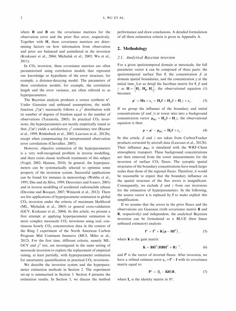
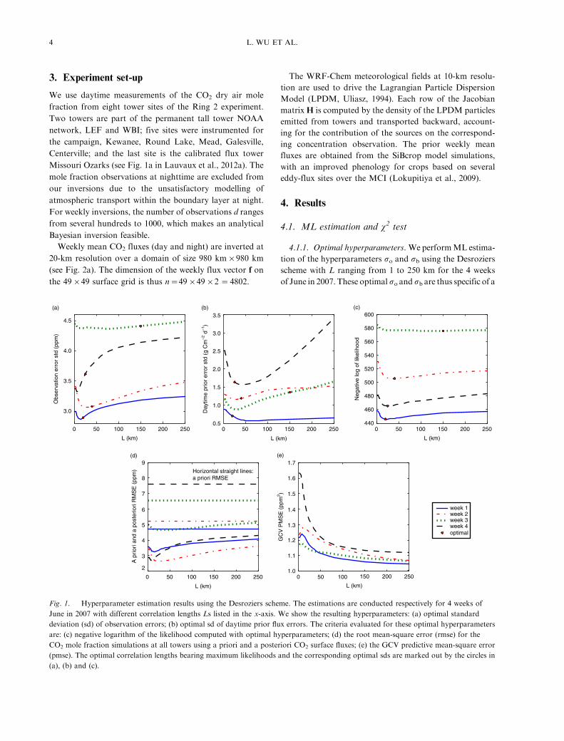
Fig. 1. Hyperparameter estimation results using the Desroziers scheme. The estimations are conducted respectively for 4 weeks of

June in 2007 with different correlation lengths Ls listed in the x-axis. We show the resulting hyperparameters: (a) optimal standard

deviation (sd) of observation errors; (b) optimal sd of daytime prior flux errors. The criteria evaluated for these optimal hyperparameters

are: (c) negative logarithm of the likelihood computed with optimal hyperparameters; (d) the root mean-square error (rmse) for the

CO2 mole fraction simulations at all towers using a priori and a posteriori CO2 surface fluxes; (e) the GCV predictive mean-square error

(pmse). The optimal correlation lengths bearing maximum likelihoods and the corresponding optimal sds are marked out by the circles in

(a), (b) and (c).

4 L. WU ET AL.

given L. We impose a fixed ratio between the nighttime and

daytime prior error sds. This ratio is set according to the

ratio between the ranges of flux variations at day and night.

The optimal so figures (Fig. 1a) are close to the default

values (3�5 ppm in summer) obtained by diagnosing the

atmospheric transport error due to incorrect vertical mixing,

flux aggregations and the misrepresentation of Eulerian

dynamics by the Lagrangian model (Lauvaux et al., 2012b).

In contrast, the optimal daytime sb figures (Fig. 1b) are far

smaller than the default value (10 g C m�2 d�1 (Lauvaux

et al., 2012b)). The resulting large so/sb ratios imply that the

inversions using optimal error variances are less constrained

by the observations than the default case.

With the default error variances, the atmospheric trans-

port error is underestimated. For instance, the vertical

transport errors may be insufficiently accounted for or the

prescribed spatiotemporal covariance structure may not

well represent the correlations in the errors of the con-

tinuous hourly observations for the Ring 2 experiment. In

midsummer, this area experiences very strong storms, and

during dry season, two severe droughts affected some parts

of the Midwest in August. The WRF convective scheme

may have difficulty simulating these events correctly,

which results in large transport errors. Detailed diagnostics

of the transport error is in process using WRF multi-

physics ensembles compared with observations (e.g. radio-

sounding and surface data). This is an important related

subject but beyond the scope of this article.

For each Balgovind correlation length L, we verified that

the ML estimate of so and sb (Fig. 1a and b) assures

44°N

42°N

40°N

38°N

(c)

GALESROUND

MEADWBI

CENTER

MIS

LEF

98°W 96°W 94°W 92°W 90°W 88°W

–0.3

–0.6

–0.9

–1.2

0.3

0.0

0.6

0.9

1.2 44°N

42°N

40°N

38°N

98°W 96°W 94°W 92°W 90°W 88°W

(d)

GALESROUND

MEADWBI

CENTER

MIS

LEF

0.30.40.5

0.60.70.80.91.0

0.20.10.0

44°N

42°N

40°N

38°N

(a)

GALESROUND

MEADWBI

CENTER

MIS

LEF

0.0

–0.3

–0.6

–0.9

–1.2

–1.5

–1.8

–2.1

98°W 96°W 94°W 92°W 90°W 88°W

44°N

42°N

40°N

38°N

98°W 96°W 94°W 92°W 90°W 88°W

(b)

GALESROUND

MEADWBI

CENTER

MIS

LEF

0.75

–0.75

–1.00

0.50

–0.50

0.25

–0.25

0.00

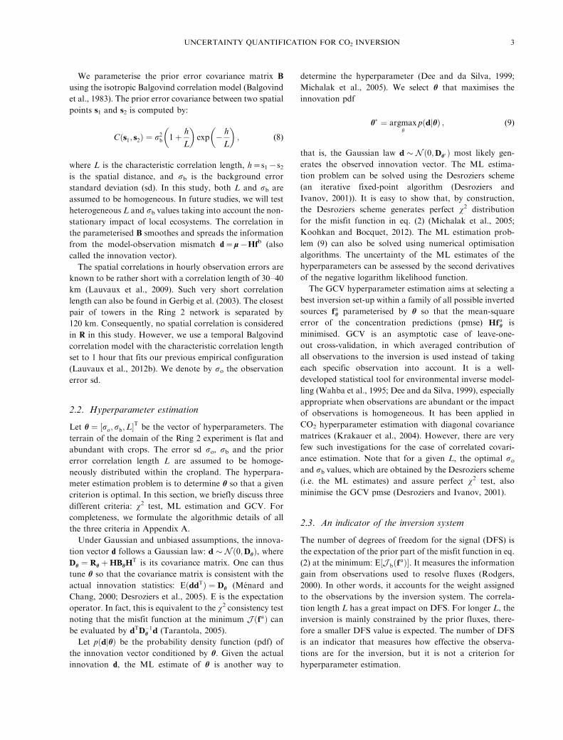
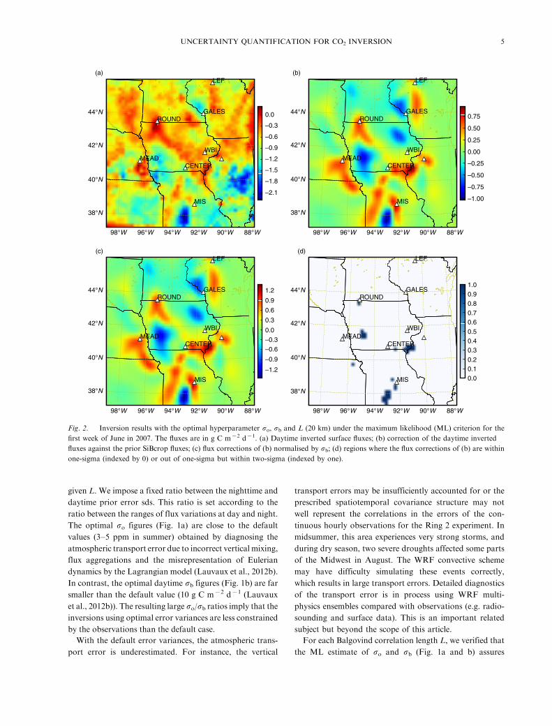
Fig. 2. Inversion results with the optimal hyperparameter so, sb and L (20 km) under the maximum likelihood (ML) criterion for the

first week of June in 2007. The fluxes are in g C m�2 d�1. (a) Daytime inverted surface fluxes; (b) correction of the daytime inverted

fluxes against the prior SiBcrop fluxes; (c) flux corrections of (b) normalised by sb; (d) regions where the flux corrections of (b) are within

one-sigma (indexed by 0) or out of one-sigma but within two-sigma (indexed by one).

UNCERTAINTY QUANTIFICATION FOR CO2 INVERSION 5

perfect x2 test. We omit the x2 curves that all approach

1. Note that, in many studies, the covariance hyperpara-

meters are empirically tuned for satisfactory x2 tests.

The ML estimate of L defines the most plausible prior

error covariance that adapts to the innovation sample

under the assumption of isotropic Balgovind correlation in

prior flux errors. Most optimal L values (read the minimal

negative logarithm likelihoods in Fig. 1c) are rather short:

between 20 and 45 km. There is one exceptionally long

optimal L of 150 km for the third week of June, for which

the observation error increase is the strongest (largest so/sbratio read from Fig. 1a and b). In this case, the signal from

the surface fluxes is highly affected by the atmospheric

transport error, so that it is difficult to retrieve meaning-

ful spatial prior correlation structure. The corresponding

negative likelihood curve in Fig. 1c is plainly flat with very

small curvature at the ML estimate. The ML estimation in

this case is highly uncertain.

To quantitatively account for the uncertainty of the ML

estimates, we compute the second derivatives of the nega-

tive logarithm likelihood function and construct its Hessian

matrix. The inverse of that Hessian matrix provides an

approximation of the covariance matrix for the ML esti-

mate (see Appendix B for algorithmic details). We list the

standard deviations for the ML estimates in Table 1. In

summary, the ML estimation does not support long spatial

correlations in prior flux errors that are usually assumed,

for example, 300 km in Lauvaux et al. (2012a). This result

confirms the global prior error estimation results obtained

by objective statistics of the differences between CO2

flux observations and flux simulations using a terrestrial

ecosystem model (Chevallier et al., 2012).

We preliminarily assess the robustness of our estimates

of L using a longer temporal correlation length of 2 hours

(default 1 hour) for R. The resulting new optimal L is

50 km with high uncertainty (also a flat, negative log like-

lihood curve in Supplementary file). Other error covariance

structures could also be possible.

In addition to the Desroziers method, we also tested

other iterative methods that adopt non-linear optimisation

algorithms (either gradient-based or gradient-free) to solve

the ML estimation problem numerically. We found that, in

most cases, they provide estimates consistent with those

obtained using the Desroziers method but occasionally get

trapped into local optima for the estimation of L given

certain initial parameter values (results omitted). There-

fore, it is desirable to perform the Desroziers method

for different L values enumerated ranging from 1 to

250 km.

4.1.2. Inversions using optimal hyperparameters. We per-

form inversions using all the L-specific optimal so and sb

values. The short optimal correlation length (e.g. L�20

km for the first week of June) prevents the information to

propagate far from the towers within the flux domain

through the inversion (see the daytime flux corrections in

Fig. 2b). In Fig. 1d, we show the root mean-square error

(rmse) for the CO2 mole fraction simulations averaged over

all towers using prior and inverted CO2 surface fluxes. The

a posteriori rmses are substantially improved compared

with the a priori rmses. Localising the observation impact

(short optimal Ls) is beneficial to inversion in terms of rmse

reduction for the dependent data.

The inverted fluxes obtained using the optimal short

L and corresponding optimal so and sb are physically

relevant (e.g. no significant positive fluxes at daytime in

Fig. 2a). Using a long L (e.g. 200 km) and its corresponding

optimal so and sb (therefore perfect x2 test) often leads

to unrealistic inverted fluxes. For instance, for the case of

week 3, we observed very positive daytime inverted fluxes,

and for the cases of weeks 2 and 4, we observed many

negative nighttime inverted fluxes (figures omitted). More-

over, Lauvaux et al. (2012a) have performed the leave-one-

tower-out cross-validation for long L and found almost no

gain in concentration rmse at validation towers. In addi-

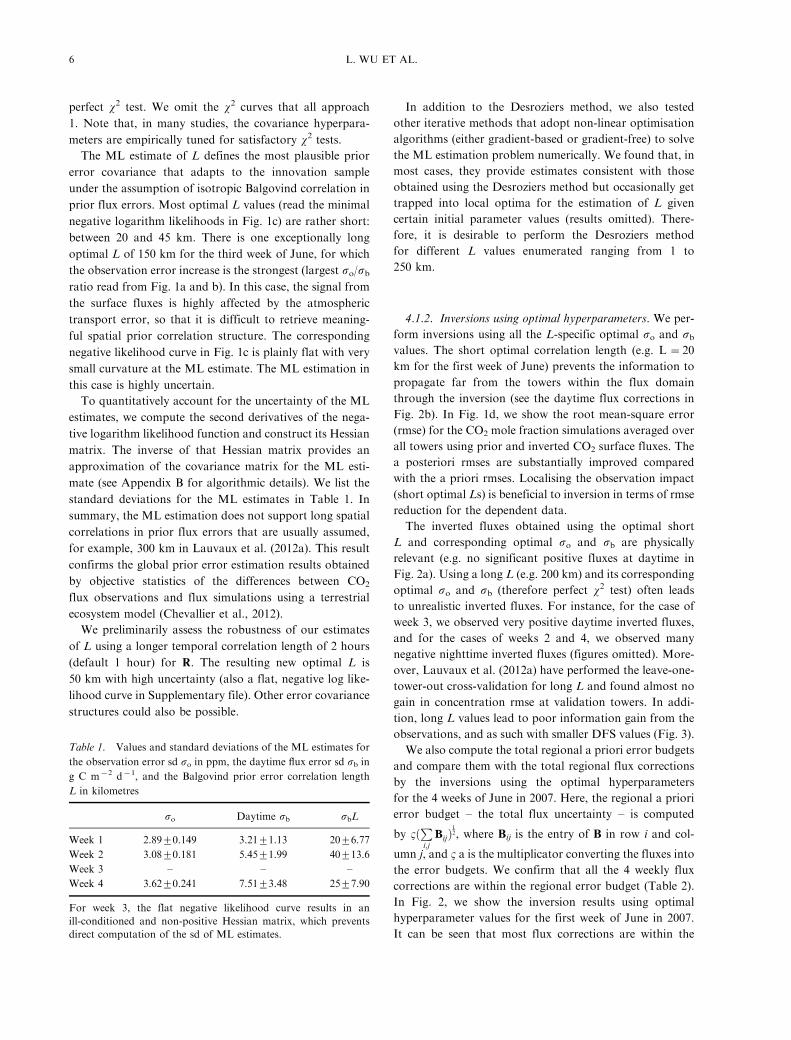
tion, long L values lead to poor information gain from the

observations, and as such with smaller DFS values (Fig. 3).

We also compute the total regional a priori error budgets

and compare them with the total regional flux corrections

by the inversions using the optimal hyperparameters

for the 4 weeks of June in 2007. Here, the regional a priori

error budget � the total flux uncertainty � is computed

by 1ðPi;j

BijÞ12, where Bij is the entry of B in row i and col-

umn j, and 1 a is the multiplicator converting the fluxes into

the error budgets. We confirm that all the 4 weekly flux

corrections are within the regional error budget (Table 2).

In Fig. 2, we show the inversion results using optimal

hyperparameter values for the first week of June in 2007.

It can be seen that most flux corrections are within the

Table 1. Values and standard deviations of the ML estimates for

the observation error sd so in ppm, the daytime flux error sd sb in

g C m�2 d�1, and the Balgovind prior error correlation length

L in kilometres

so Daytime sb sbL

Week 1 2.8990.149 3.2191.13 2096.77

Week 2 3.0890.181 5.4591.99 40913.6

Week 3 � � �Week 4 3.6290.241 7.5193.48 2597.90

For week 3, the flat negative likelihood curve results in an

ill-conditioned and non-positive Hessian matrix, which prevents

direct computation of the sd of ML estimates.

6 L. WU ET AL.

one-sigma range (Fig. 2c and d): the inversion system

with the optimal hyperparameter values is statistically

consistent.

We do not extend this evaluation to longer time scales,

for example, the month or the year, since we perform

weekly inversions without the possibility to correlate errors

from 1 week to the next, even though there is some evidence

that such long correlations exist (Chevallier et al., 2012):

neglecting temporal correlations leads to underestimating

the a priori error budgets for periods longer than a week.

4.2. General cross-validation

Krakauer et al. (2004) reported a successful application of

GCV in global CO2 hyperparameter estimation for the case

of diagonal covariance matrices; however, the effectiveness

of GCV for the case of correlated covariance matrices is

still unknown. Recall that for a given L, the GCV esti-

mate of so and sb coincides with the ML estimate.

Consequently, we use the ML estimate of so and sb to

compute the GCV pmses for different Ls values. It is seen

that GCV fails to find an optimal L (Fig. 1e). We can see

two possible reasons for this failure: (1) GCV is a criterion

of approximate leave-one-out cross-validation based on

the assumption of a uniform impact of the observations,

but the Ring 2 network is spatially too sparse and too

heterogeneous for such approximation; (2) GCV is very

sensitive to the error structure in R (Wahba et al., 1995) but

in our case R is empirically determined.

5. Discussion and conclusions

Direct approaches to quantify the uncertainty of prior

fluxes are based on the statistics of flux misfits. For

instance, Rodenbeck et al. (2003) intercompared several

terrestrial and ocean models, and Chevallier et al. (2006,

2012) compared ecosystem model simulations with eddy-

covariance flux measurements. These statistics only par-

tially explore the space of uncertainties, because this space

can be sampled by few models in the former case and by

few measurements in the latter one. Additional information

is needed to verify and complement the direct approaches.

The proposed hyperparameter estimation methodology is

one such effort that analyses the signal from mole fraction

measurements to estimate the flux uncertainty. To put it

more generally, this methodology selects the uncertainty

hyperparameters that optimise some desired property of

the inversion system, like maximising the likelihood of

observation (ML), the x2 consistency under the Gaussian

paradigm, and GCV of inverted fluxes. This approach

also benefits the assignment of observation error statistics:

observation error statistics account for the errors of the

underlying transport model, of which estimation has been

another long-standing issue (e.g. Gurney et al., 2002). The

computational cost of optimising the inversion system is of

one order of magnitude larger than that of the inversion

and has hampered such developments so far.

We have examined the ML estimation, the x2 test and

the GCV in estimating the variances and the correlation

lengths of the error covariance matrices for prior fluxes and

concentration observations in a mesoscale setting. Real,

continuous hourly CO2 concentration data were assimi-

lated to invert weekly CO2 fluxes at a 20-km resolution.

The correlation length L characterises the errors in the

modelling of the ecophysiological processes that generate

the fluxes. Its estimation based on CO2 mole fraction

measurements only may not always be appropriate. In this

article, we have enumerated different L values, and for each

L value an ML estimation is conducted. We interpret these

results with great caution.

DF

S

L (km)

120

100

80

60

40

20

00 50 100 150 250200

week 1week 2week 3week 4

Fig. 3. Numbers of DFS with respect to correlation length

L in prior flux errors for 4 weeks of June in 2007. Inversions

are performed using optimal hyperparameters obtained

by the Desroziers scheme. X-axis lists different correlation

length Ls.

Table 2. Comparison between the total regional error budget

of a priori fluxes (‘budget’ column) and the total regional flux

correction by inversions (‘correction’ column) for the 4 weeks of

June in 2007

Optimal L (km) Budget (Gg C) Correction (Gg C)

week 1 20 227 201

week 2 40 742 601

week 3 150 2546 674

week 4 25 658 621

The optimal hyperparameters obtained by the Desroziers method

(marked out by the circles in Fig. 1a and b) are used for this

comparison.

UNCERTAINTY QUANTIFICATION FOR CO2 INVERSION 7

For a given correlation length L in prior flux errors, the

ML and GCV estimates of the error variances coincide and

assure perfect x2 test. In addition, the misspecifications of

default observation error variance values were corrected

to represent the atmospheric transport error. When L was

to be estimated jointly with the error variances, the ML

estimate did not support long spatial correlations (e.g. an

optimum of 20 km for the first week of June 2007), which is

consistent with the estimation results at the global scale

obtained in the direct approach (Chevallier et al., 2012). In

contrast, GCV failed to provide optimal L values. In the

same geophysical data-sparse context, Bocquet (2012) also

found the ML estimation superior to GCV for the inverse

modelling of radionuclide release. We further diagnosed

the flux error budget and the flux corrections by the

inversions using optimal hyperparameters. The optimised

inversions produced satisfactory statistical consistency,

in spite of the limitations of the Gaussian modelling

framework (that may be less valid for mesoscale regional

inversions than for global ones).

We have evaluated the robustness of our study by con-

ducting hyperparameter estimation for other periods in

the summer of 2007. The results show consistent patterns

(see Supplementary file): (1) GCV fails to estimate L, and

the ML estimate does not support long L; and (2) when the

atmospheric transport error is significant, it is difficult to

identify a meaningful optimal L from the flat likelihood

curve.

The hyperparameter estimation appears to be a promis-

ing alternative to empirical tuning methods for uncertainty

quantification. In principle, its computational load drama-

tically increases with the observation number, if the huge

covariance matrices have to be evaluated. However, hyper-

parameter estimation in such a situation should not be

considered to be a daunting task. Randomisation techni-

ques exist to avoid huge matrix computations using per-

turbed variational inversions, and the ML estimation could

be done with few iterations. Both have already been

successfully demonstrated in meteorological applications

(Desroziers and Ivanov, 2001; Chapnik et al., 2004).

The boundary and initial concentrations have been cor-

rected by aircraft data to decrease the bias of the system.

Removing the remaining bias leads to maximal 10%

relative differences in inverted fluxes near the towers.

Hence, the potential bias has very limited impact on our

weekly inversions. For longer periods, such bias will play a

more important role on the estimation of the regional

budget and should be estimated jointly with the fluxes. By

imposing longer spatial correlations in flux errors for

inversions, the distribution of the flux corrections at finer

spatial scales may be less precise; however, jointly with

bias corrections, the regional budget can be satisfactorily

estimated (Schuh et al., 2013).

Careful attention and further investigations are needed

for the full-scale mesoscale application of hyperparameter

estimation. The space�time density of the observation net-

work may limit the estimation of some hyperparameters,

like L, due to insufficient statistics. In our case, a denser

network than the one studied here would be helpful for

more robust estimates. To mitigate the effect of a sparse

network, some reliable knowledge about the hyperpara-

meters may be necessary, especially when many hyperpara-

meters are to be estimated. For instance, in our study, we

used information from model simulations to impose the

initial and lateral boundary conditions and the ratio

between daytime and nighttime flux error variances rather

than estimating them. However, when such hypotheses are

not reasonable, the hyperparameter estimation may yield

misleading results. Data density is also desirable to leave

some mole fraction measurements out of the estimation

process for the validation of the optimised hyperpara-

meters. Direct flux observations can also serve for this

purpose.

6. Acknowledgements

This study is a contribution to the MSDAG project

supported by the French Agence Nationale de la Recherche

grant ANR-08-SYSC-014. The first author is currently

funded by the industrial chaire BridGES supported by

the Universite de Versailles Saint-Quentin-en-Yvelines,

the Commissariat a l’Energie Atomique et aux Energies

Renouvelables, the Centre National de la Recherche

Scientifique, Thales Alenia Space and Veolia.

7. Appendix

A. Criteria for hyperparameter estimation

Suppose the surface CO2 flux vector f 2 Rn can be related

to the observation (or receptor) vector l 2 Rd as:

l ¼ Hf þ EEo ; (A1)

where eo is an error vector with zero mean, andH is a linear

operator that includes the atmospheric transport.

The Bayesian inversion specifies the a posteriori prob-

ability density function (pdf) given information on the

prior and the observation according to Bayes’ rule:

pðfjlÞ ¼ pðljfÞpðfÞpðlÞ

; (A2)

where pð�Þ is the probability density of a sample.

8 L. WU ET AL.

In CO2 inversions, the prior estimate of f is usually

assumed to follow a Gaussian law Nðfb;BÞ:

pðfÞ ¼exp � 1

2ðf � fbÞTB�1ðf � fbÞ

h iffiffiffiffiffiffiffiffiffiffiffiffiffiffiffiffiffið2pÞnjBj

p ; (A3)

where fb is a prior guess vector, and B ¼ EðEEbEETb Þ is the

covariance matrix for the unbiased prior error EEb ¼ fb � f.

Here, the expectation operator is denoted by E. The

Gaussian assumption is convenient for the computation

of the likelihood of observations given fluxes:

pðljfÞ ¼ pðl�HfÞ ¼exp � 1

2ðl�HfÞTR�1ðl�HfÞ

h iffiffiffiffiffiffiffiffiffiffiffiffiffiffiffiffiffið2pÞd jRj

q ;

(A4)

where R ¼ E ðl�HfÞðl�HfÞTh i

is the observation error

covariance matrix.

Let h ¼ ½ro; rb;L�T

be the vector of hyperparameters.

The objective of the hyperparameter estimation problem is

to find u so that a given criterion J(u) is optimal for the

estimation of the surface fluxes f.

A1. Maximum likelihood estimation

In the ML hyperparameter estimation, one chooses u that

maximises its conditional pdf p hjlð Þ. If we assume a

constant evidence p(m) (a normalising denominator) and a

uniform prior p(u) (no available prior information on u),

according to Bayes’ rule:

p hjlð Þ ¼ p ljhð Þp hð Þp lð Þ

; (A5)

the posterior p hjlð Þ is proportional to the likelihood p ljhð Þ:

p hjlð Þ / p ljhð Þ : (A6)

The maximum likelihood estimation problem is then:

h� ¼ argmaxh

p ljhð Þ : (A7)

When pðljhÞ reaches its maximum at u*, the pdf pðljhÞ isthe most peaked, which indicates that the observation m is

the least uncertain.

In the context of analytical Bayesian inversion, the

likelihood pðljhÞ can be further evaluated by

p ljhð Þ ¼Z

pðljf; hÞpðfjhÞdf

¼exp � 1

2ðl�HfbÞTD�1

h ðl�HfbÞh i

ð2pÞd2jDhj

12

; (A8)

where Dh ¼ Rh þHBhHT is the covariance matrix of the

innovation vector d ¼ l�Hfb. The corresponding nega-

tive logarithm likelihood to be minimised is:

LðhÞ ¼ � ln pðljhÞ

¼ 1

2ln jDhj þ

1

2ðl�HfbÞTD�1

h ðl�HfbÞ þ C; (A9)

where C is an irrelevant constant.

For a given L, supposing the true error covariance

matrices are of the forms Bt�sbB and Rt�s8R where B

and R are computed using fixed default so and sb, the

hyperparameter vector then becomes u�[s8, sb]T. The

Desroziers scheme (Desroziers and Ivanov, 2001) can

be used to iteratively solve the necessary condition (zero-

gradient) of the maximum likelihood estimation problem

rhL ¼ 0; (A10)

as follows:

so ¼ 2JoðfaÞTr Id �HKh

� � ; (A11)

sb ¼ 2JbðfaÞTr KhH� � ; (A12)

where

Kh ¼ BhHTD�1h ; (A13)

JoðfÞ ¼1

2ðl�HfÞTR�1ðl�HfÞ ; (A14)

JbðfÞ ¼1

2ðf � fbÞTB�1ðf � fbÞ: (A15)

Provided sa and sb are of the same order of magnitude (i.e.

the default so and sb are not far from the true values), the

Hessian matrix of the negative log likelihood function

equation (A9) has positive diagonal terms and negligible

non-diagonal terms (Chapnik et al., 2004). This assures us

that the Desroziers scheme reaches one minimum of the

negative log likelihood function. There exists efficient

randomisation algorithms to compute the trace terms

in eqs. (A11) and (A12) for very large observation sets

(Desroziers and Ivanov, 2001). This is a typical configura-

tion in variational CO2 inversions (Chevallier et al., 2010),

for which it is computationally infeasible to use the original

maximum likelihood formalism equation (A9) for hyper-

parameter estimation. Furthermore, the Desroziers scheme

could terminate with satisfactory solutions in a few itera-

tions (Chapnik et al., 2004).

In general, the different sources of uncertainties are

entangled in the inversion system, which complicates the

uncertainty quantification problem. If R and B have equal

correlation length in the observation space (HBHT�aR

with 0Ba �R), then eqs. (A11) and (A12) are identical. In

this case, the Desroziers scheme fails to provide a solution

UNCERTAINTY QUANTIFICATION FOR CO2 INVERSION 9

(Chapnik et al., 2004). In our study, since R is taken to be

spatially uncorrelated, R and HBHT have distinct correla-

tion structures, which favours the identification of the error

variances.

The Desroziers scheme stems from the consistency

check of the inversion system by statistical diagnosis of

the inverted variables, for example, E½JbðfaÞ� ¼ 12TrðKHÞ.

The term Jb(fa) is a satisfactory approximation of its

expected value E[Jb(fa)], if the time window for inversions

is long enough to include a large batch of observations

for sufficient statistics. This approximation implies an

ergodicity assumption for the retrieval of the desired

knowledge (the hyperparameter values in our case) from

the statistics of one single realisation of the underlying

geophysical process. Similarly, the negative log likelihood

function relies also on one realisation of m and fb. The

hyperparameter estimation is thus data specific; however,

it is reasonable to expect that the estimation results are

robust for similar scenarios, for example, summer time

weekly inversions.

Other iterative methods exist to numerically minimise the

negative log likelihood function equation (A9). These nu-

merical optimisation methods can be either gradient-based

(e.g. the augmented Lagrangian method) or gradient-free

(e.g. constrained optimisation by linear approximations). In

this study, we used the NLopt library (http://ab-initio.mit.

edu/nlopt) for non-linear optimisation.

A2. Degrees of freedom for the signal and x2

The number of degrees of freedom for the signal (DFS) can

be defined as (Rodgers, 2000):

DFS ¼ E fa � fb� �T

B�1h fa � fb� �h i

; (A16)

where E is the expectation operator over the errors in the

prior fluxes and the observations. The DFS measure the

relative correction of fa to fb. Under Gaussian assumptions,

the DFS can be computed by TrðAhÞ where Ah ¼ KhH is the

averaging kernel matrix. This equals to Tr Bh � Pah

� �B�1

h

� ,

which measures the relative reduction of uncertainty for the

BLUE analysis.

It is well known that if the Gaussian assumptions on

prior and observation errors are valid, the quantity

v2ðfaÞ ¼ ðl�HfaÞTR�1h ðl�HfaÞ þ ðfa � fbÞTB�1

h ðfa � fbÞ(A17)

follows a x2 probability density of which the number of

degrees of freedom equals the number of the observation d.

Rayner et al. (1999), Rodenbeck et al. (2003), Lauvaux

et al. (2012b) empirically selected the hyperparameter

values by checking the x2 consistency of fa.

For the Desroziers scheme using one single realisation of

a batch of observations, by eqs. (A11), (A12), (A14), (A15),

we have

v2ðfaÞ ¼ 2JoðfaÞso

þ 2JbðfaÞsb

¼ d : (A18)

This means that the parameter u* obtained using the

Desroziers scheme bears the perfect x2 test for that batch of

data (see Koohkan and Bocquet, 2012 for a direct fixed-

point method that leads to the perfect x2 test).

A3. Cross-validation

An ideal criterion accounting for the inversion performance

is the predictive mean-square error (pmse):

PðhÞ ¼ 1

dkH f � fað Þk2; (A19)

where f is the assumed true flux vector and fa is the inverted

flux vector using hyperparameter u. This criterion is not

practical since f is unknown. However, other criteria can be

derived when f is replaced by fa but the expectation E PðhÞ½ �

remains the least affected. The general cross-validation

(GCV) pmse is one such criterion.

One popular cross-validation criterion is the leave-one-

out cross-validation error:

QðhÞ ¼ 1

d

Xd

i¼1

Hifai � lið Þ2 : (A20)

Here fai is the inverted flux vector using d�1 observations

with the i-th observation mi removed from inversion, andHi

the i-th row of H associated with mi. The computation of

Q(u) is time consuming since d times of inversion are

needed. Using the ordinary cross-validation (OCV) identity

(Wahba, 1990), this could be reduced to only one time of

inversion by replacing Q(u) with

Q0ðhÞ ¼ 1

d

Xd

i¼1

Hifa � li

1� ½HKh�ii

!2

; (A21)

where the matrix HKu is the resolution matrix (Rodgers,

2000) with its i-th diagonal element ½HKh�ii indicating the

number of DFS elucidated by assimilating i-th observation

mi Unfortunately, Q?(u) has a disturbing dependence on the

ordering of the observations (½HK�ii changes if the rows of

H are permuted).

The GCV pmse

VðhÞ ¼1dkl�Hfak2

R�1

1dTr Id �HKh

� �� 2(A22)

is an approximation of Q?(u), in which the averaged

contribution of all observations to inversion TrðHKhÞ=d

10 L. WU ET AL.

is used instead of the specific observation contribution

½HKh�ii so that some ordering invariance properties could

be achieved. GCV has the property that its expectation is

close to that of P(u). Note that we have formulated V(u) in

R�1-norm. In this case, the scaled observational error is

expected to be white, which would favour the separation of

noise from signal for GCV hyperparameter estimation.

Nevertheless, if the covariance structure of R is unrealistic,

the scaled observation error would not be white. This may

significantly degrade the GCV performance (Wahba et al.,

1995).

For a given L, the hyperparameters so and sb obtained

using the Desroziers scheme minimise the GCV pmse

(Desroziers and Ivanov, 2001).

B. Uncertainty of the hyperparameter estimates

The ML estimate u* has several desired properties in the

asymptotic limit of very large samples. For instance, the

distribution of u* approaches normality, and the covar-

iance of this normal distribution can be approximately

computed by the inverse of the Hessian matrix H (the

second partial derivatives) of the negative log likelihood

function equation (A9) at the ML estimate u*. We refer to

statistics texts (for instance Efron and Hinkley, 1978;

Lindsey, 1996) for more details.

In geophysical applications, it would be demanding

for large samples, since the underlying phenomena are so

complex that an observation never repeats under identical

conditions. However, it is still possible to perform para-

meter estimation for a single sample of one realisation of

the geophysical process (Dee, 1995). This would result in

covariance models more consistent with the actual innova-

tions. For reliable accuracy, Dee and da Silva (1999) suggest

that an order of 100 observations is required to estimate

a single parameter. In our study, more observations are

available than required by this empirical rule.

Let us formulate explicitly the ij-th element of the

Hessian matrix H of the negative log likelihood function

equation (A9) as:

HijðhÞ ¼@2LðhÞ@hi@hj

: (B1)

By linear algebra and matrix calculus, we have

HijðhÞ ¼ �1

2TrðD�1

h Dh;jD�1h Dh;iÞ

þ 1

2TrðD�1

h Dh;ijÞ �1

2dTD�1

h Dh;ijD�1h d

þ dTD�1h Dh;jD

�1h Dh;iD

�1h d;

(B2)

where

Dh;i ¼@Dh

@hi

; (B3)

Dh;ij ¼@2Dh

@hi@hj

; (B4)

are the first and second derivatives of the innovation

covariance matrix Du.

The Hessian matrix at the ML estimate u* has a geo-

metric interpretation. It characterises the local curvature of

the negative log likelihood function. The magnitude of a

change in L resulting from a perturbation of u* along the

eigen-direction of H is proportional to the corresponding

eigenvalue. Therefore, the Hessian matrix is related to the

accuracy of the ML estimate. The approximate covariance

matrix for the ML estimate is simply the inverse of the

Hessian matrix at u*

Hðh�Þ�1: (B5)

The small curvature (at the ML estimate) of the flat

negative log likelihood curve for week 3 in June 2007

in Fig. 1c indicates that the estimation is inaccurate

and bears large uncertainties. The corresponding Hessian

matrix could be ill-conditioned and non-positive definite.

In this case, higher order moments may be needed to clarify

these large uncertainties.

The negative log likelihood function in eq. (A9) is correct

only under Gaussian assumptions with known covariance

structures. When these assumptions do not hold, solutions

from minimising eq. (A9) will not be guaranteed to be

the ML estimates, but result in parametric covariance

models that are more consistent with data. To account for

uncertainties due to the unknown covariance structure,

that is the robustness of the estimates, one can perform a

sensitivity analysis for the parameter estimation problem

under different assumptions. For instance, correlation

models other than Balgovind could be tested; the back-

ground error covariance matrix Bu could be anisotropic;

and the structure of the observation error covariance

matrix Ru may take on more realistic forms. Detailed

analysis on robustness would be beyond the scope of this

article but we will keep in mind for future studies.

References

Balgovind, R., Dalcher, A., Ghil, M. and Kalnay, E. 1983. A

stochastic-dynamic model for the spatial structure of forecast

error statistics. Mon. Wea. Rev. 111, 701�722.Bocquet, M. 2012. An introduction to inverse modelling and

parameter estimation for atmospheric and oceanic sciences. In:

Advanced Data Assimilation for Geosciences (eds. E. Blayo, M.

Bocquet and E. Cosme). Oxford University Press, Les Houches

School of Physics.

UNCERTAINTY QUANTIFICATION FOR CO2 INVERSION 11

Bousquet, P., Peylin, P., Ciais, P., Quere, C. L., Friedlingstein, P.

and co-authors. 2000. Regional changes in carbon dioxide fluxes

of land and oceans since 1980. Science. 290(5495), 1342�1346.Chapnik, B., Desroziers, G., Rabier, F. and Talagrand, O. 2004.

Properties and first application of an error-statistics tuning

method in variational assimilation. Q. J. Roy. Meteorol. Soc.

130, 2253�2275.Chevallier, F. 2007. Impact of correlated observation errors on

inverted CO2 surface fluxes from OCO measurements. Geophys.

Res. Lett. 34, L24804. DOI: 10.1029/2007GL030463.

Chevallier, F., Ciais, P., Conway, T. J., Aalto, T., Anderson, B. E.

and co-authors. 2010. CO2 surface fluxes at grid point scale

estimated from a global 21 year reanalysis of atmospheric

measurements. J. Geophys. Res. 115, D21307. DOI: 10.1029/

2010JD013887.

Chevallier, F., Viovy, N., Reichstein, M. and Ciais, P. 2006. On

the assignment of prior errors in Bayesian inversions of CO2

surface fluxes. Geophys. Res. Lett. 33, L13802. DOI: 10.1029/

2006GL026496.

Chevallier, F., Wang, T., Ciais, P., Maignan, F., Bocquet, M. and

co-authors. 2012. What eddy-covariance measurements tell us

about prior land flux errors in CO2-flux inversion schemes. Glob.

Chang. Biol. 26, GB1021. DOI: 10.1029/2010GB003974.

Davoine, X. and Bocquet, M. 2007. Inverse modelling-based

reconstruction of the Chernobyl source term available for

long-range transport. Atmos. Chem. Phys. 7, 1549�1564. DOI:

10.5194/acp-7-1549-2007.

Dee, D. P. 1995. On-line estimation of error covariance para-

meters for atmospheric data assimilation. Mon. Wea. Rev. 123,

1128�1145.Dee, D. P. and da Silva, A. M. 1999. Maximum-likelihood

estimation of forecast and observation error covariance para-

meters. Part I: methodology. Mon. Wea. Rev. 127, 1835�1849.Desroziers, G., Berre, L., Chapnik, B. and Poli, P. 2005. Diagnosis

of observation, background and analysis-error statistics in

observation space. Q. J. Roy. Meteorol. Soc. 131, 3385�3396.DOI: 10.1256/qj.05.108.

Desroziers, G. and Ivanov, S. 2001. Diagnosis and adaptive tuning

of observation-error parameters in a variational assimilation. Q.

J. Roy. Meteorol. Soc. 127, 1433�1452.Efron, B. and Hinkley, D. 1978. Assessing the accuracy of the

maximum likelihood estimator: observed versus expected fisher

information. Biometrika. 65, 457�487.Gerbig, C., Lin, J. C., Wofsy, S. C., Daube, B. C., Andrews, A. E.

and co-authors. 2003. Toward constraining regional-scale fluxes

of CO2 with atmospheric observations over a continent: 2.

analysis of COBRA data using a receptor-oriented framework.

J. Geophys. Res. 108(D24), 4757. DOI: 10.1029/2003JD003770.

Gurney, K. R., Law, R. M., Denning, A. S., Rayner, P. J., Baker,

D. and co-authors. 2002. Towards robust regional estimates of

CO2 sources and sinks using atmospheric transport models.

Nature. 415, 626�630.Hansen, P. C. 2010. Discrete Inverse Problems: Insight and

Algorithms. SIAM Publishing, Philadelphia, 225 pp.

Koohkan, M. R. and Bocquet, M. 2012. Accounting for repre-

sentativeness errors in the inversion of atmospheric constituent

emissions: application to the retrieval of regional carbon

monoxide fluxes. Tellus B. 64, 19047.

Krakauer, N. Y., Schneider, T., Randerson, J. T. and Olsen, S. C.

2004. Using generalized cross-validation to select parameters in

inversions for regional carbon fluxes. Geophys. Res. Lett. 31,

L19108. DOI: 10.1029/2004GL020323.

Lauvaux, T., Pannekoucke, O., Sarrat, C., Chevallier, F., Ciais, P.

and co-authors. 2009. Structure of the transport uncertainty in

mesoscale inversions of CO2 sources and sinks using ensemble

model simulations. Biogeosciences. 6(6), 1089�1102.Lauvaux, T., Schuh, A. E., Bocquet, M., Wu, L., Richardson, S.

and co-authors. 2012a. Network design for mesoscale inversions

of CO2 sources and sinks. Tellus B. 64, 17980.

Lauvaux, T., Schuh, A. E., Uliasz, M., Richardson, S., Miles, N.

and co-authors. 2012b. Constraining the CO2 budget of the corn

belt: exploring uncertainties from the assumptions in a mesos-

cale inverse system. Atmos. Chem. Phys. 11, 337�354. DOI:

10.5194/acp-12-337-2012.

Lindsey, J. K. 1996. Parametric Statistical Inference. Oxford

University Press, Oxford, 512 pp.

Lokupitiya, E., Denning, S., Paustian, K., Baker, I., Schaefer, K.

and co-authors. 2009. Incorporation of crop phenology in

simple biosphere model (SiBcrop) to improve land�atmosphere

carbon exchanges from croplands. Biogeosciences. 6,

969�986.Menard, R. and Chang, L.-P. 2000. Assimilation of stratospheric

chemical tracer observations using a Kalman filter. Part ii:

c2-validated results and analysis of variance and correlation

dynamics. Mon. Wea. Rev. 128, 2672�2686.Michalak, A. M., Hirsch, A., Bruhwiler, L., Gurney, K. R., Peters,

W. and co-authors. 2005. Maximum likelihood estimation of

covariance parameters for Bayesian atmospheric trace gas sur-

face flux inversions. J. Geophys. Res. 110, D24107. DOI: 10.

1029/2005JD005970.

Miles, N. L., Richardson, S. J., Davis, K. J., Lauvaux, T.,

Andrews, A. E. and co-authors. 2012. Large amplitude spatial

and temporal gradients in atmospheric boundary layer CO2

mole fractions detected with a tower-based network in the

U.S. upper Midwest. J. Geophys. Res. 117, G01019. DOI:

10.1029/2011JG001781.

Rayner, P. J., Enting, I. G., Francey, R. J. and Langenfelds, R.

1999. Reconstructing the recent carbon cycle from atmospheric

CO2, d13c and O2/N2 observations. Tellus B. 51, 213�232. DOI:

10.1034/j.1600-0889.1999.t01-1-00008.x.

Rodenbeck, C., Houweling, S., Gloor, M. and Heimann, M. 2003.

CO2 flux history 1982�2001 inferred from atmospheric data

using a global inversion of atmospheric transport. Atmos. Chem.

Phys. 3, 1919�1964.Rodgers, C. D. 2000. Inverse Methods for Atmospheric Sounding:

Theory and Practice. World Scientific Publishing, Singapore,

240 pp.

Schuh, A. E., Lauvaux, T., West, T. O., Denning, A. S., Davis,

K. J. and co-authors. 2013. Evaluating atmospheric CO2

inversions at multiple scales over a highly inventoried agricul-

tural landscape. Glob. Chang. Biol. 19(5), 1424�1439. DOI:

10.1111/gcb.12141.

12 L. WU ET AL.

Tarantola, A. 2005. Inverse Problem Theory and Model Parameter

Estimation. SIAM Publishing, Philadelphia, 352 pp.

Uliasz, M. 1994, Lagrangian particle dispersion modeling in

mesoscale applications. In: Environmental Modeling II (ed. P.

Zannetti). Computational Mechanics Publications, Southampton,

pp. 71�102.Vogel, C. R. 2002. Computational Methods for Inverse Problems.

SIAM Publishing, Philadelphia, 183 pp.

Wahba, G. 1990. Spline Models for Observational Data. SIAM

Publishing, Philadelphia, 180 pp.

Wahba, G., Johnson, D. R., Gao, F. and Gong, J. 1995. Adaptive

tuning of numerical weather prediction models: randomized

GCV in three- and four-dimensional data assimilation. Mon.

Wea. Rev. 123, 3358�3370.

Winiarek, V., Bocquet, M., Saunier, O. and Mathieu, A. 2012.

Estimation of errors in the inverse modeling of accidental release

of atmospheric pollutant: application to the reconstruction of

the cesium-137 and iodine-131 source terms from the Fukushima

Daiichi power plant. J. Geophys. Res. 117, D05122. DOI:

10.1029/2011JD016932.

Wu, L., Bocquet, M., Lauvaux, T., Chevallier, F., Rayner, P. and

co-authors. 2011. Optimal representation of source-sink fluxes

for mesoscale carbon dioxide inversion with synthetic data. J.

Geophys. Res. 116, D21304. DOI: 10.1029/2011JD016198.

UNCERTAINTY QUANTIFICATION FOR CO2 INVERSION 13