Identifying and Fusing Duplicate Features for Data Mining

Hortensia C. Barcelos, Mariana Recamonde-Mendoza, Viviane P. Moreira

1Instituto de Informatica – Universidade Federal do Rio Grande do Sul (UFRGS)Caixa Postal 15.064 – 91.501-970 – Porto Alegre – RS – Brazil

Abstract. This work addresses the problem of identifying and fusing duplicatefeatures in machine learning datasets. Our goal is to evaluate the hypothesisthat fusing duplicate features can improve the predictive power of the data whilstreducing training time. We propose a simple method for duplicate detection andfusion based on a small set of features. An evaluation comparing the duplicatedetection against a manually generated ground truth obtained F1 of 0.91. Then,the effects of fusion were measured on a mortality prediction test. The resultswere inferior to the ones obtained with the original dataset. Thus we concludedthat the investigated hypothesis does not hold.

1. Introduction

The problem of identifying duplicate features has been extensively studied in the Databasefield in the context of data integration. The literature on schema matching, data deduplica-tion, and record linkage is prolific with many solutions having been proposed throughoutthe years [Madhavan et al., 2001, Do and Rahm, 2002, Storer et al., 2008, Meister et al.,2012, Bhattacharya and Getoor, 2004, Christen, 2008]. However, within the fields of ma-chine learning (ML) and data mining, this problem is not well studied since most work isdevoted to devising techniques for dimensionality reduction and feature selection.

The duplicate features issue appears in situations in which data comes from differ-ent sources (as with data integration) but also in large datasets such as medical databases.MIMIC-III [Johnson et al., 2016], for example, is a very important healthcare dataset usedin hundreds of scientific works. It contains many events that were recorded as separatefeatures (e.g., arterial pressure is recorded as arterial pressure, arterial bp mean, arterialblood pressure mean, and arterial bp mean #2), although they share the same semantics.Whenever different sources or information systems are involved in data collection, MLtasks are subject to duplication and redundancy between features, making it necessaryto create a denser representation of information with minimal loss of quality. Duplicatefeatures lead to data sparsity (i.e., missing feature values), which is known to have anegative impact on ML algorithms. Moreover, not only fitting high dimensional data iscomputationally expensive, but it is also prone to overfitting due to high complexity.

In this context, identifying and fusing duplicate features could potentially bringgains in terms of prediction quality and computational costs by reducing data sparsity anddimensionality. We note, however, that duplicate features fusion differs from dimension-ality reduction techniques based on feature extraction (e.g., Principal Component Analy-sis). Whereas the latter produces new features in a lower-dimensional space by creatinglinear combinations of the original variables, regardless of their semantics, feature fusionaims at preserving the underlying semantics of the data by aggregating information forclosely-related features in a domain-specific fashion.

Manually evaluating a dataset in search for duplicate features is unfeasible, aspairwise comparisons are required. A small dataset with 100 features would require anexpert to evaluate almost 5K pairs. Thus, to minimize the effort from the domain special-ist, feature fusion methods should be able to learn the fusion rules from a small annotatedsample. The model derived from the sample can then be applied to the complete dataset.

The goal of this paper is to evaluate the hypothesis that fusing duplicate featurescan improve the predictive power of the data whilst reducing training time. In order todo that, we propose a set of fusion features that capture evidences from different sources.These evidences are fed to a classification algorithm. We compared three types of al-gorithms: a traditional method (Random Forest) [Breiman, 2001]; and two methods thatrequire only positive instances, the Positive Unlabeled method SKC [Bao et al., 2018] andOne Class Classification Support Vector Machine (OSVM) [Scholkopf et al., 2000].

The fusion methods were applied to MIMIC-III [Johnson et al., 2016] in two ways.First, we performed an intrinsic evaluation to measure the quality of the duplicate featuredetection. The results have shown that duplicate detection can achieve an F1 of 0.91 usingour proposed features. Then, we ran an extrinsic evaluation to assess the effects of featurefusion on a mortality prediction task. With the extrinsic evaluation, we test our hypothesisregarding the benefit of feature fusion. These results do not support the hypothesis sincelearning from the original (unfused) dataset yielded better classification results.

2. BackgroundIn this section, we summarize some important concepts in the context of the problem offusing duplicate features.

2.1. Supervised Learning AlgorithmsThe context of this work involves supervised learning algorithms, i.e., a subclass of MLin which a model is learned from annotated training instances and is further applied toclassify unseen data. Several algorithms have been proposed for this task and are widelyemployed [Mitchell, 1997]. Below we briefly review the algorithms adopted in our work.

Naıve Bayes (NB) is a probabilistic classifier based on Bayes’ theorem, with anassumption of independence among predictors. NB computes the posterior probability ofeach possible class y given our prior knowledge, represented by the input feature vectorX = (x1, x2, ..., xN) from which conditional probabilities are estimated. The class thatmaximizes the posterior probability is returned by the classifier [Mitchell, 1997].

Random Forest (RF) is a tree-based ensemble algorithm, well known for its pos-itive impact on performance variance. RF groups several Decision Trees with differentbranch structures that generate different paths. The tree outputs are combined in such away that the RF output is generated from the class that appeared most often among theset of tree outputs present in the forest [Breiman, 2001]. Thus, it is necessary to configurethe parameters such as (i) number of trees to be used, (ii) the measure of the quality of asplit, such as gini for the Gini impurity and entropy for the information gain and (iii) themaximum depth of the tree.

2.2. One-class ClassificationOne-class Classification (OCC) works with the premise that the classifier should identifywhether the new instance belongs to a target class. It is applicable to problems where neg-

ative instances represent failures, anomalies, or errors, making negative instances difficultto obtain. For this reason, OCC defines the classification limit around the positive class inorder to allow the classifier to accept as much data as possible as a positive class and tominimize the probability of accepting data outside the target class. The difficulty lies indeciding, using only positive data, how narrow this boundary should be around the dataand what attributes of these instances should be used to assist in the separation betweenpositive and negative classes [Khan and Madden, 2014].

The OCC-Support Vector Machine (OSVM) algorithm is a modification of theSupport Vector Machine (SVM) method that works according to the OCC premise, beingused mainly in problems of anomaly detection. Scholkopf et al. [2000] developed analgorithm that returns +1 if the instance is within a small region that captures most of thedata, which would be considered as the target class that share similar characteristics, and-1 for data outside that region. This way, when generating a hyperplane that separatesthe space, this function is used when the apprentice machine receives a new instance andmust evaluate in which region it will be. Depending on the region, it will be labeledas positive or negative. This type of classifier prioritizes learning the characteristics ofthe positive class; for this reason its training phase uses only positive instances. Theparameters that need to be configured for OSVM are the kernel type (linear, poly, rbf,sigmoid), the kernel coefficient (γ), and the limit between the fraction of training errorsand the support vectors.

2.3. Positive-Unlabeled LearningPositive-Unlabeled Learning (PUL) presents a different approach to training data: it as-sumes that all labeled input data is positive and that the remaining unlabeled data forthe problem can be either positive or negative. PUL methods are different because bothpositive and unlabeled samples are used during the training phase. Bao et al. [2018] pro-posed the Set Kernel Classifier (SKC) method based on PUL, which dealt with this typeof classification along with another learning problem, called Multiple Instance Learning.Their work is based on sets of instances called bags that are labeled as follows: if there isat least one positive instance, then the bag is labeled as positive; if there are no positiveinstances, then the bag is labeled as negative.

Two important parameters that must be configured when using PUL are the classprior, i.e., the probability of the positive class, and the regularization term (λ). The classprior, in PUL problems, cannot be calculated since only a small sample labeled as positiveis known during classifier training. Thus, during their experiments, Plessis et al. [2015]used variations of the class prior, however, they suggest that these parameters should beknown or estimated at training time.

2.4. Classifier EvaluationClassifier evaluation is done by comparing the predicted labels against ground truth la-bels. Some of the most widely used evaluation metrics are:• Accuracy, which measures the proportion of the correctly classified instances.• Precision, which measures what proportion of the instances that were classified as be-longing to a given class, in fact belong to that class.• Recall, which measures what proportion of the instances that belong to a given classthat were assigned to the class by the classifier. The recall of the positive class is also

called TR Rate.• F1, which is the harmonic mean between precision and recall.• FP Rate, which measures the proportion of false positives.• FN Rate, which measures the proportion of false negatives.

In order to reduce the effects of variability, cross-validation (CV) [Kohavi, 1995]is typically employed. It consists in splitting the dataset into k-folds, with k-1 folds beingused for training and the remaining fold used for testing. Training and test folds changek times so that all folds are used for testing. Then results of the k-folds are averaged.

3. Related Work

Feature fusion is a widely used method in the area of image classification and recognition.Sun et al. [2004] proposed a feature fusion method based on Canonical Correlation Anal-ysis, which uses the correlation of two groups of features as for fusion and to eliminateredundant information between features. This reduction allowed only essential featuresof the image to be maintained, showing good performance in classification tasks. Scalzoet al. [2008] used the Feature Fusion Hierarchies model, which combines feature fusionand decision fusion, generated by an evolutionary algorithm for the classification of gen-der in images. This model significantly reduced the classification error when comparedwith PCA. Perez et al. [2012] demonstrated that feature fusion after feature selection us-ing mutual information measures improves the performance of gender classification inimages. Lin et al. [2015] proposed a fusion algorithm called Heterogeneous StructureFusion that deals with the distribution of each feature and similarity between features. Itwas evaluated in image classification, face recognition, shape analysis, and infrared im-agery. Their results revealed that this algorithm outperformed feature fusion methods forclassification problems. Our work differs from feature fusion in image classification dueto the nature of our features. Here, our scope is structured data. This work is the first touse feature fusion to fuse duplicate features.

The task of feature fusion shares similarities with schema matching, one of thephases of data integration that aims at identifying matching elements across differentschemas so that they can be merged. Even though both methods have similar goals,the phases of (i) checking the data to detect the matches between the attributes and (ii)joining the attributes that match; are different. Gal [2006] and Sutanta et al. [2016] pointto the dependence that schema matching tools have on the need for user interaction andhow attached these tools are to the Data Base Management System for which they weredesigned. There is a vast literature on this topic [Bilke and Naumann, 2005, Do and Rahm,2002, Bernstein et al., 2011]. However, schema matching solutions are designed to workwith two or more schemas to integrate. In our work, the duplicate features are consideredwithin a single schema.

4. Detecting and Fusing Duplicate Features

Table 1 shows a small example of duplicate and non-duplicate features. The data refersto health measurements of patients. This example is useful to illustrate the differencebetween redundant and duplicate features. Features “heart rate” and “Hr rate” are du-plicate, i.e., they refer to the same measurement and should thus be fused. On the otherhand, “temperature C” and “Temp F” (which record the patient’s body temperature in

Table 1. Examples of duplicate and non-duplicate features

f1 f2 f3 f4 f5 f6 f7 f8 f9Subject temperature C heart rate NBP[systolic] Hr rate Manual BP [systolic] Temp F Venous PVCO2 Venous PVO2

1 30 71 100 35 382 100 120 97 40 423 32 75 135 32 41

Celsius and Fahrenheit, respectively) are not duplicate as they use different units of mea-surement. Fusing them would merge values coming from different distributions, whichin turn would add noise to the learning tasks. These two features are redundant, as theyare likely to be highly correlated. Thus, a feature selection algorithm, such as a wrappermethod, is likely to discard one of them. In this paper, we focus on duplicate and not onredundant features.

The problem addressed here can be more formally described as follows. Givena set of original features F = {f1, f2, ..., fn}, 〈fi, fj〉 is a pair of features, where fi ∈F, fj ∈ F and i 6= j. Each original feature fi is associated with a name li and a setof values Vi = {v1, v2, ..., vm}. The task of identifying duplicate features determineswhether fi and fj are duplicate, i.e., refer to the same actual feature. Then, feature fusionis responsible for merging the original features that have been identified as duplicates.Each duplicate pair 〈fi, fj〉 is fused to became a new feature fh = fi ⊕ fj , where ⊕ is apreviously defined aggregating function and depends on the type of data. A new name lhis created and associated to this new fused feature fh.

Duplicate feature detection relies in a set of features that are fed into a classifier,which creates a model from an initial set of labeled instances. Once the model is created,it can be used to classify all pairs of features from the dataset. This is a very challengingtask because of a number of reasons:

• The number of pairs of original features to analyze can be very large, which makesthe task computationally expensive. To help mitigate this problem, the number offeatures should be kept small.• The model will need to learn from a small set of labeled instances, since labeling

is a labor-intensive task that needs to be performed by a domain-specialist.• The number of negative pairs (i.e., pairs of features that are not duplicate) is much

larger than the number of positive pairs. This yields an extremely unbalanceddataset, which typically poses challenges to learning algorithms. In this sense, theuse of learning schemes that rely solely on positive instances (such as the onespresented in Sections 2.2 and 2.3) is desirable.• Capturing the semantic similarity of the attributes is very difficult. For example,

the pair 〈f8, f9〉 from Table 1 has similar names and their values lie within thesame range. However, they are not duplicate as one refers to Carbon Dioxide andthe other to Oxygen. This example reinforces the idea that using different sourcesof evidence is necessary.

4.1. Duplicate Detection

Duplicate detection is modeled as a binary classification problem. For a given pair oforiginal features fi and fj , the task of the classifier is to assign a label stating whether fiand fj are duplicates. The decision as to whether any pair of original features is duplicate

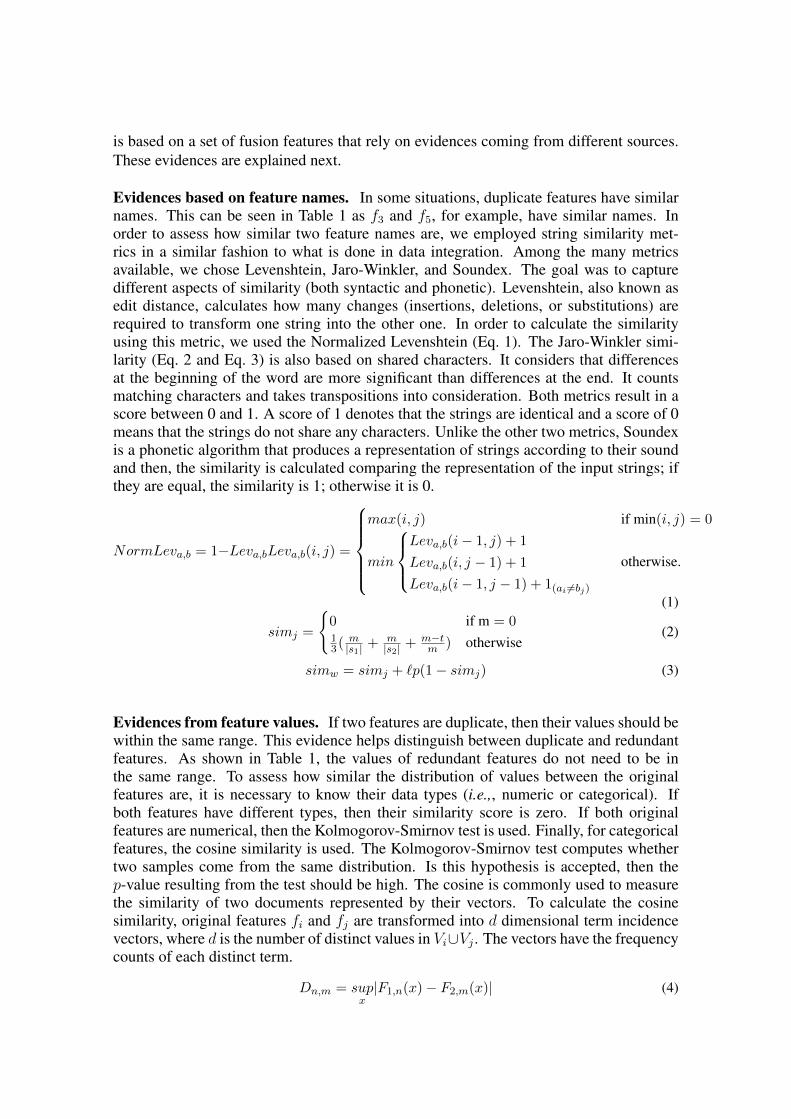
is based on a set of fusion features that rely on evidences coming from different sources.These evidences are explained next.

Evidences based on feature names. In some situations, duplicate features have similarnames. This can be seen in Table 1 as f3 and f5, for example, have similar names. Inorder to assess how similar two feature names are, we employed string similarity met-rics in a similar fashion to what is done in data integration. Among the many metricsavailable, we chose Levenshtein, Jaro-Winkler, and Soundex. The goal was to capturedifferent aspects of similarity (both syntactic and phonetic). Levenshtein, also known asedit distance, calculates how many changes (insertions, deletions, or substitutions) arerequired to transform one string into the other one. In order to calculate the similarityusing this metric, we used the Normalized Levenshtein (Eq. 1). The Jaro-Winkler simi-larity (Eq. 2 and Eq. 3) is also based on shared characters. It considers that differencesat the beginning of the word are more significant than differences at the end. It countsmatching characters and takes transpositions into consideration. Both metrics result in ascore between 0 and 1. A score of 1 denotes that the strings are identical and a score of 0means that the strings do not share any characters. Unlike the other two metrics, Soundexis a phonetic algorithm that produces a representation of strings according to their soundand then, the similarity is calculated comparing the representation of the input strings; ifthey are equal, the similarity is 1; otherwise it is 0.

NormLeva,b = 1−Leva,bLeva,b(i, j) =

max(i, j) if min(i, j) = 0

min

Leva,b(i− 1, j) + 1

Leva,b(i, j − 1) + 1

Leva,b(i− 1, j − 1) + 1(ai 6=bj)

otherwise.

(1)

simj =

{0 if m = 013(

m|s1| +

m|s2| +

m−tm ) otherwise

(2)

simw = simj + `p(1− simj) (3)

Evidences from feature values. If two features are duplicate, then their values should bewithin the same range. This evidence helps distinguish between duplicate and redundantfeatures. As shown in Table 1, the values of redundant features do not need to be inthe same range. To assess how similar the distribution of values between the originalfeatures are, it is necessary to know their data types (i.e.,, numeric or categorical). Ifboth features have different types, then their similarity score is zero. If both originalfeatures are numerical, then the Kolmogorov-Smirnov test is used. Finally, for categoricalfeatures, the cosine similarity is used. The Kolmogorov-Smirnov test computes whethertwo samples come from the same distribution. Is this hypothesis is accepted, then thep-value resulting from the test should be high. The cosine is commonly used to measurethe similarity of two documents represented by their vectors. To calculate the cosinesimilarity, original features fi and fj are transformed into d dimensional term incidencevectors, where d is the number of distinct values in Vi∪Vj . The vectors have the frequencycounts of each distinct term.

Dn,m = supx|F1,n(x)− F2,m(x)| (4)

Evidences from co-occurrence. If two original features fi and fj are duplicate, thentheir values tend to co-occur infrequently, i.e., instances do not normally have values forboth fi and fj simultaneously. This can be seen in Table 1, as duplicate features 〈f3, f5〉and 〈f4, f6〉 do not co-occur. To quantify feature co-occurrence, we compute the JaccardSimilarity between them, according to Eq. 5. The intersection between fi and fj is thenumber of instances in the dataset which have values for both fi and fj . When analyzinga database with temporal data, the definition of intersection can be adapted to account forevents that occurred within a time interval (i.e., the same day, hour, etc.).

Jaccard(fi, fj) =fi ∩ fjfi ∪ fj

(5)

4.2. Feature Fusion

Once the duplicate features have been identified, the next step is to fuse them. The fusionprocess needs to deal with merging a possibly large number of original features. Forexample, if the pairs 〈f1, f2〉 and 〈f2, f3〉 are both identified as duplicate, then features f1,f2, and f3 should be fused. In order to prevent an undesirably large cascading of fusions,we employ a threshold θ that specifies the maximum number of original features to bemerged into a single one. In this process, original features that have a higher probabilityof being duplicate should be prioritized. Hence, the pairs of original features that wereidentified as duplicate are sorted in decreasing order of a score s that calculates the averageof the values of the fusion features. Then, fusion processes the pairs with highest s scoresfirst, merging them in groups of at most θ features.

In order to fuse the values of the original features, aggregating functions (i.e., av-erage, minimum, maximum, mode) are used to transform the feature distribution into asingle value. Hence, from a set of instances X = {x1, x2, ..., xm}, its processing cre-ates xp = (fp,1[g], fp,2[g], ..., fp,n[g]), where g is the aggregating function used for eachoriginal feature and xp ∈ X .

5. Intrinsic EvaluationThis evaluation aims to verify how well the classification methods perform on labelingeach pair of original features as duplicate or not i.e., here we perform an intrinsic evalu-ation of the methods. The comparison was made using RF, SKC (a PUL method) [Baoet al., 2018], and OSVM [Scholkopf et al., 2000]. In the next subsections, we describedata preparation for these experiments, model training procedures, and their results.

5.1. Materials and Methods

Data. Our data comes from the MIMIC-III v1.4 database [Johnson et al., 2016], whichcontains over 40K patients and thousands of variables. The patients are medical andsurgical who were admitted to an Intensive Care Unit at a hospital in Boston-USA. Eachpatient has a number of associated events (i.e., measurements for vital signs, values oflaboratory tests, etc.). These events are the original features in our setting. This datasetwas chosen because it has events stored with different ids but that represent the sameevent. This is a known issue that has made its organizers list the identified occurrencesin a repository1. For example, there are six features referring to Systolic Arterial Blood

1https://github.com/MIT-LCP/mimic-code/blob/master/concepts/firstday/vitals-first-day.sql

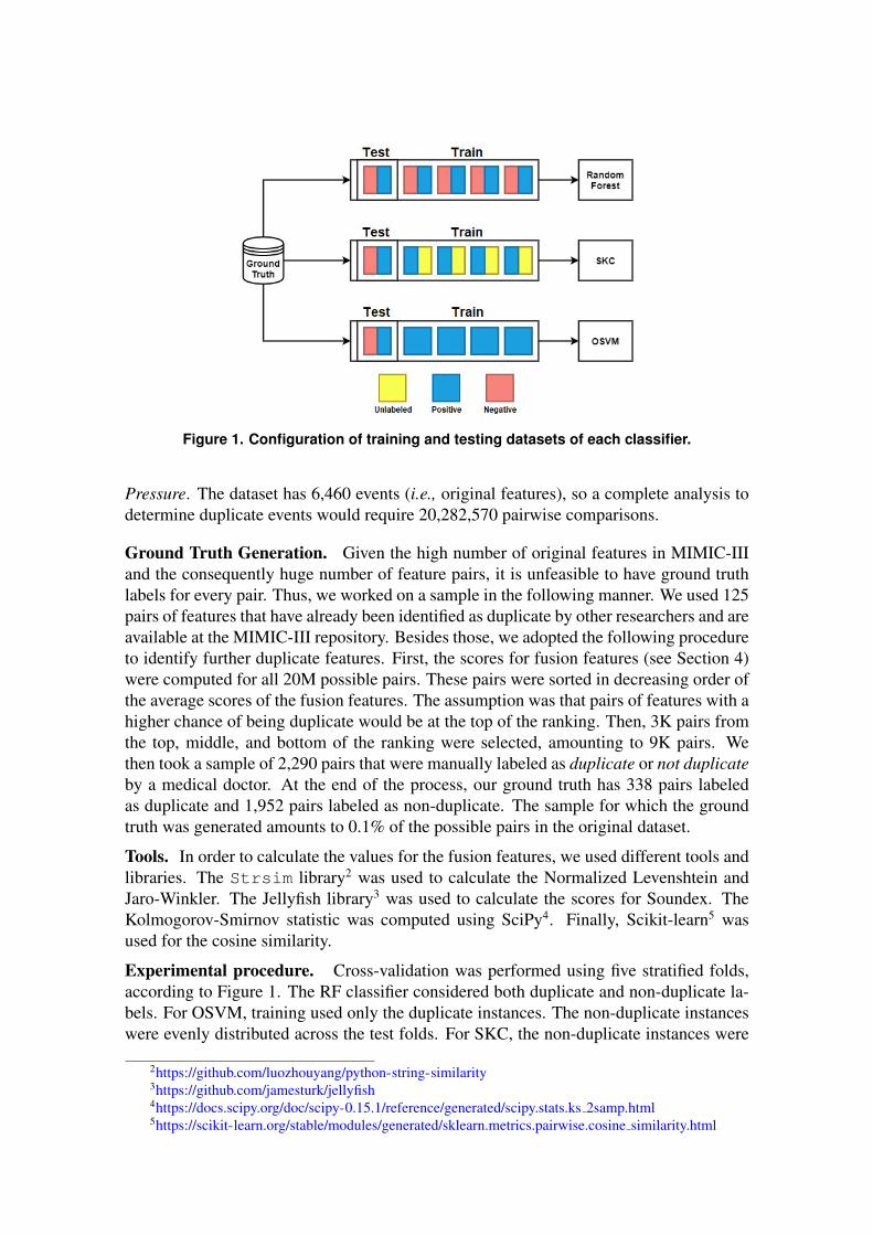
Figure 1. Configuration of training and testing datasets of each classifier.

Pressure. The dataset has 6,460 events (i.e., original features), so a complete analysis todetermine duplicate events would require 20,282,570 pairwise comparisons.

Ground Truth Generation. Given the high number of original features in MIMIC-IIIand the consequently huge number of feature pairs, it is unfeasible to have ground truthlabels for every pair. Thus, we worked on a sample in the following manner. We used 125pairs of features that have already been identified as duplicate by other researchers and areavailable at the MIMIC-III repository. Besides those, we adopted the following procedureto identify further duplicate features. First, the scores for fusion features (see Section 4)were computed for all 20M possible pairs. These pairs were sorted in decreasing order ofthe average scores of the fusion features. The assumption was that pairs of features with ahigher chance of being duplicate would be at the top of the ranking. Then, 3K pairs fromthe top, middle, and bottom of the ranking were selected, amounting to 9K pairs. Wethen took a sample of 2,290 pairs that were manually labeled as duplicate or not duplicateby a medical doctor. At the end of the process, our ground truth has 338 pairs labeledas duplicate and 1,952 pairs labeled as non-duplicate. The sample for which the groundtruth was generated amounts to 0.1% of the possible pairs in the original dataset.

Tools. In order to calculate the values for the fusion features, we used different tools andlibraries. The Strsim library2 was used to calculate the Normalized Levenshtein andJaro-Winkler. The Jellyfish library3 was used to calculate the scores for Soundex. TheKolmogorov-Smirnov statistic was computed using SciPy4. Finally, Scikit-learn5 wasused for the cosine similarity.

Experimental procedure. Cross-validation was performed using five stratified folds,according to Figure 1. The RF classifier considered both duplicate and non-duplicate la-bels. For OSVM, training used only the duplicate instances. The non-duplicate instanceswere evenly distributed across the test folds. For SKC, the non-duplicate instances were

2https://github.com/luozhouyang/python-string-similarity3https://github.com/jamesturk/jellyfish4https://docs.scipy.org/doc/scipy-0.15.1/reference/generated/scipy.stats.ks 2samp.html5https://scikit-learn.org/stable/modules/generated/sklearn.metrics.pairwise.cosine similarity.html

Table 2. Results for the Intrinsic Evaluation – Feature Fusion

OSVM SKC RF

TP Rate/Recall 0.654 0.766 0.867Precision 0.781 0.615 0.958Accuracy 0.922 0.895 0.975FP Rate 0.032 0.083 0.007FN Rate 0.346 0.234 0.133F1 0.712 0.682 0.910

considered unlabeled for training and the folds were divided into positive and unlabeledbags with three instances each. During test, the non-duplicate instances remained negativeand the fold was divided into bags with only one instance.

After evaluating several parameters configurations for the algorithms, the bestones were defined as follows. OSVM: RBF kernel, kernel coefficient γ = 0.25, and thelimit between the fraction of training errors and the support vectors nu = 0.35. SKC:training error rate (λ) = 0.0001 and the positive class probability (prior) = 0.15. RF: num-ber of trees n trees = 250, the function that measures the quality of the division criterion= Gini (Index), and max depth = None.

5.2. Results

Table 2 shows the results for the intrinsic evaluation. RF was the best performer acrossall metrics. These results indicate that having negative instances helps the distinctionbetween duplicate and non-duplicate features, despite the existing class imbalance. In acomparison between OSVM and SKC, the former is better in terms of precision, accuracy,FP rate, and F1, while the latter is better in terms of TP Rate and FN Rate.

In order to assess whether the algorithms agreed on the instances they labeled asduplicate/not duplicate, we plotted the intersections of the predictions of each methodw.r.t each other and the ground truth (i.e., the ”True Positive” group). The Venn diagramsare shown in Figure 2. We can see that 63% (212/338) of the duplicate features were iden-tified by all three algorithms. For the non-duplicate features, the agreement was higher,reaching 91% (1767/1952).

Once the classification models were learned using the annotated data, they wereused to label the complete dataset containing all possible pairs of original features. Thenumber of instances labeled in each class by the three methods are shown in Table 3.

Table 3. Number of instances (i.e., pair of original features) labeled as duplicateand not duplicate by each classifier.

OSVM SKC RF

Duplicate 4,264,367 2,984,812 4,730,359Not Duplicate 16,595,913 17,875,468 16,129,921

We also performed a manual analysis of the errors made by the classifiers. As ageneral tendency, we noticed that false positives tended to have highly similar names anddistributions such as temperature celsius and temperature f. As for falsenegatives, they typically either have highly similar names and high co-occurrence such

(a) Duplicate (b) Not Duplicate

Figure 2. Diagrams showing the intersection among classifiers’ predictions andthe ground truth for the (a) positive (duplicate) and (b) negative (not dupli-cate) examples in our dataset.

as tpa#mg/hr and tpa#2 mg/hr or they have low similarity between their names,zero co-occurrence, and high similarity of distribution such as glucose (70-105)and bloodglucose.

6. Extrinsic EvaluationThis evaluation aims to assess the impact that feature fusion has on a classification task,i.e., an extrinsic evaluation. The task used in the tests is mortality prediction, an importanttopic in medical informatics.

6.1. Materials and Methods

Data. As our original features come from MIMIC-III (described in Sec. 5), the data usedfor this evaluation also comes from this same dataset. Subjects were adult patients and theinstances had only events and measurements from the first 24 hours of their last hospitalstay. The task is to predict whether a patient will die based on information collected earlyat the hospital stay. We took a random sample of 13,171 patients (out of the 32,507 in thecomplete dataset). The sample has 4,563 deceased and 8,608 surviving patients.

Tools. Weka [Hall et al., 2009] was used for running the classifiers.

Experimental Procedure. We used the Naıve Bayes classifier with ten-fold CV. Thethreshold for feature fusion was θ = 15. Experimental runs were done with each methodfor feature fusion and two baselines – the original (unfused) dataset and also fusing onlythe features that we identified as duplicate in the ground truth. Due to computationallimitations only Naıve Bayes classifier was used in this evaluation.

6.2. Results

The results for the mortality prediction task are shown in Table 4. We can see that allmethods of feature fusion had a negative impact on the quality of the prediction. A pairedt-test was used to compare F1 results (which are normally distributed) across the ten foldsfor each original and fused dataset. The results indicated that the reduction is statisti-cally significant using α = 0.01. Even the fusion based on the ground truth lowered the

Table 4. Results for the Extrinsic Evaluation – Mortality Prediction

Metric Original Ground Truth OSVM SKC RF

TP Rate/Recall 0.773 0.772 0.755 0.759 0.762Precision 0.713 0.712 0.699 0.700 0.700Accuracy 0.647 0.646 0.633 0.633 0.631FP Rate 0.419 0.420 0.432 0.434 0.438FN Rate 0.227 0.228 0.245 0.241 0.238F1 0.655 0.654 0.641 0.640 0.639Training Time (seconds) 2.615 2.463 1.000 1.107 1.098#Features 6,108 6,010 2,063 2,119 2,328

scores. This fact leads us to conclude that the hypothesis that fusing duplicate featurescan improve the predictive power of the data could not be validated in our experiments.

As expected, as a result of the reduction in the number of features, model trainingwas much faster on the fused datasets. Training time was reduced to almost a third of thetime as a result of the reduction in the number of features by the same proportion. We cansee here that the duplicate detection process had many false positives since the duplicatesactually represent a much smaller fraction of the set of original features.

7. ConclusionIn medical informatics, a recurrent problem found in datasets is duplicate features derivedfrom similar, decentralized data sources, which results in greater dimensionality withoutproportionally increasing the value of the data. The hypothesis that drove this work wasthat fusing duplicate features could result in better generalization power of classifiers.Although the results for the intrinsic evaluation were quite high, the extrinsic evaluationshowed that fusion was too aggressive. The duplicate detection phase should be furtherinvestigated, looking for more evidences that can assist in the process of labeling duplicatefeature pairs. Training time was improved for extrinsic evaluation, but predictive powerfailed in surpassing baselines values.

We note, however, that our work had some important limitations. First, our testswere done over a single dataset. Despite being a real, challenging medical dataset, exper-iments on other datasets are needed to further investigate our hypothesis and improve ourunderstanding on this topic. Moreover, further experiments could be performed exploringdifferent proportions of labeled data for the duplicate features (which in our work wasonly 0.1% of the possible pairs in the original dataset), as well as new features aimingat reducing false positives. Finally, whereas lower dimensionality decreases model com-plexity, which in turn contributes to a better generalization power, we could not investigatemore deeply in our scenario due to the lack of independent data.

Acknowledgements. This work was partially supported by CAPES Finance Code 001.

ReferencesHan Bao, Tomoya Sakai, Issei Sato, and Masashi Sugiyama. Convex formulation of multiple

instance learning from positive and unlabeled bags. Neural Networks, 105:132 – 141, 2018.Philip A Bernstein, Jayant Madhavan, and Erhard Rahm. Generic schema matching, ten years

later. Proc. of the VLDB Endowment, 4(11):695–701, 2011.

Indrajit Bhattacharya and Lise Getoor. Iterative record linkage for cleaning and integration.In ACM SIGMOD Workshop on Research Issues in Data Mining and Knowledge Discovery,DMKD, page 11–18, 2004.

Alexander Bilke and Felix Naumann. Schema matching using duplicates. In International Con-ference on Data Engineering (ICDE), pages 69–80, 2005.

Leo Breiman. Random forests. Machine learning, 45(1):5–32, 2001.Peter Christen. Febrl -: An open source data cleaning, deduplication and record linkage system

with a graphical user interface. In International Conference on Knowledge Discovery and DataMining, page 1065–1068, 2008.

Hong-Hai Do and Erhard Rahm. Coma—a system for flexible combination of schema matchingapproaches. In International Conference on Very Large Databases, pages 610–621, 2002.

Avigdor Gal. Why is schema matching tough and what can we do about it? ACM Sigmod Record,35(4):2–5, 2006.

Mark Hall, Eibe Frank, Geoffrey Holmes, Bernhard Pfahringer, Peter Reutemann, and Ian H Wit-ten. The weka data mining software: an update. ACM SIGKDD explorations newsletter, 11(1):10–18, 2009.

Alistair EW Johnson, Tom J Pollard, Lu Shen, H Lehman Li-wei, Mengling Feng, MohammadGhassemi, Benjamin Moody, Peter Szolovits, Leo Anthony Celi, and Roger G Mark. Mimic-iii,a freely accessible critical care database, 2016.

Shehroz S Khan and Michael G Madden. One-class classification: taxonomy of study and reviewof techniques. The Knowledge Engineering Review, 29(3):345–374, 2014.

Ron Kohavi. A study of cross-validation and bootstrap for accuracy estimation and model selec-tion. International Joint Conference on Artificial Intelligence, 1995.

Guangfeng Lin, Guoliang Fan, Xiaobing Kang, Erhu Zhang, and Liangjiang Yu. Heterogeneousfeature structure fusion for classification. Pattern Recognition, 2015.

Jayant Madhavan, Philip A Bernstein, and Erhard Rahm. Generic schema matching with cupid.In VLDB, volume 1, pages 49–58, 2001.

Dirk Meister, Jurgen Kaiser, Andre Brinkmann, Toni Cortes, Michael Kuhn, and Julian Kunkel.A study on data deduplication in hpc storage systems. In International Conference on HighPerformance Computing, Networking, Storage and Analysis, pages 1–11, 2012.

Tom M. Mitchell. Machine Learning. McGraw-Hill, mar 1997.Claudio Perez, Juan Tapia, Pablo Estevez, and Claudio Held. Gender classification from face im-

ages using mutual information and feature fusion. International Journal of Optomechatronics,2012.

Marthinus Christoffel Du Plessis, Gang Niu, and Masashi Sugiyama. Convex formulation forlearning from positive and unlabeled data. In International Conference on Machine Learning,volume 37, pages 1386–1394, jun 2015.

Fabien Scalzo, George Bebis, Mircea Nicolescu, Leandro Loss, and Alireza Tavakkoli. Featurefusion hierarchies for gender classification. International Conference on Pattern Recognition,2008.

Bernhard Scholkopf, Robert C Williamson, Alex J Smola, John Shawe-Taylor, and John C Platt.Support vector method for novelty detection. In Advances in neural information processingsystems, pages 582–588, 2000.

Mark W. Storer, Kevin Greenan, Darrell D.E. Long, and Ethan L. Miller. Secure data deduplica-tion. In International Workshop on Storage Security and Survivability, page 1–10, New York,NY, USA, 2008.

Quan-Sen Sun, Sheng-Gen Zeng, Yan Liu, Pheng-Ann Heng, and De-Shen Xia. A new method offeature fusion and its application in image recognition. Pattern Recognition, 2004.

Edhy Sutanta, Retantyo Wardoyo, Khabib Mustofa, and Edi Winarko. Survey: Models and pro-totypes of schema matching. International Journal of Electrical and Computer Engineering,2016.