Embed Size (px)
Citation preview
Technische Universität Dresden
Impedance Sensors for Fast Multiphase Flow
Measurement and Imaging
Dipl.-Ing. Marco Jose da Silva
von der Fakultät Elektrotechnik und Informationstechnik der
Technischen Universität Dresden
zur Erlangung des akademischen Grades eines
Doktoringenieurs
(Dr.-Ing.)
genehmigte Dissertation
Vorsitzender: Herr Prof. Dr.-Ing. habil. J. Czarske
Gutachter: Herr Prof. Dr.-Ing. habil. G. Gerlach Tag der Einreichung: 05.05.2008
Herr PD Dr.-Ing. habil. U. Hampel Tag der Verteidigung: 11.08.2008
Herr Prof. Dr. W. Yang
Technische Universität Dresden
Impedance Sensors for Fast Multiphase Flow
Measurement and Imaging
Marco Jose da Silva, M.S.E.E.
Electrical and Computer Engineering Department at the
Technische Universität Dresden
to receive the academic degree
Doktoringenieur
(Dr.-Ing.)
approved dissertation
Chairman: Prof. Dr.-Ing. habil. J. Czarske
Referees: Prof. Dr.-Ing. habil. G. Gerlach Submission: 05.05.2008
PD Dr.-Ing. habil. U. Hampel Public defense: 11.08.2008
Prof. Dr. W. Yang

"And though I have the gift of prophecy, and understand all mysteries, and all knowledge; and though I have all faith, so as to remove mountains, but have not love, I am nothing."
(I Corinthians 13:2, The Bible)

Information about the electronic version of this thesis
This PhD thesis has also been published as book ISBN 978-3-940046-99-4 by
TUDpress (http://www.tud-press.de) in the series "Dresden Contributions to Sensor
Technology" edited by Prof. G. Gerlach.
i
Abstract
Multiphase flow denotes the simultaneous flow of two or more physically distinct and
immiscible substances and it can be widely found in several engineering applications,
for instance, power generation, chemical engineering and crude oil extraction and
processing. In many of those applications, multiphase flows determine safety and
efficiency aspects of processes and plants where they occur. Therefore, the
measurement and imaging of multiphase flows has received much attention in recent
years, largely driven by a need of many industry branches to accurately quantify,
predict and control the flow of multiphase mixtures. Moreover, multiphase flow
measurements also form the basis in which models and simulations can be developed
and validated.
In this work, the use of electrical impedance techniques for multiphase flow
measurement has been investigated. Three different impedance sensor systems to
quantify and monitor multiphase flows have been developed, implemented and
metrologically evaluated. The first one is a complex permittivity needle probe which
can detect the phases of a multiphase flow at its probe tip by simultaneous
measurement of the electrical conductivity and permittivity at up to 20 kHz
repetition rate. Two-dimensional images of the phase distribution in pipe cross
section can be obtained by the newly developed capacitance wire-mesh sensor. The
sensor is able to discriminate fluids with different relative permittivity (dielectric
constant) values in a multiphase flow and achieves frame frequencies of up to 10 000
frames per second. The third sensor introduced in this thesis is a planar array sensor
which can be employed to visualize fluid distributions along the surface of objects and
near-wall flows. The planar sensor can be mounted onto the wall of pipes or vessels
and thus has a minimal influence on the flow. It can be operated by a conductivity-
based as well as permittivity-based electronics at imaging speeds of up to

ii Abstract
10 000 frames/s. All three sensor modalities have been employed in different flow
applications which are discussed in this thesis.
The main contribution of this research work to the field of multiphase flow
measurement technology is therefore the development, characterization and
application of new sensors based on electrical impedance measurement. All sensors
present high-speed capability and two of them allow for imaging phase fraction
distributions. The sensors are furthermore very robust and can thus easily be
employed in a number of multiphase flow applications in research and industry.
iii
Acknowledgments
This work is the result of my research activities at the Institute of Safety Research,
Forschungszentrum Dresden-Rossendorf e.V. (FZD), Germany, between 2004 and
2007. I would like to thank all the people who have made my work with this thesis
easier, better and more fun.
First and foremost, I would like to thank God for giving me wisdom and guidance
throughout my life.
I am extremely grateful to my supervisor at FZD, Dr. Uwe Hampel, for his
support, orientation and friendship during these years. He has provided me with the
opportunity to work on interesting current scientific and engineering topics.
I also express my deeply gratitude to my supervisor at TUD, Prof. Gerald Gerlach,
for accepting me as one of his PhD students and also for the support, orientation and
kind assistance along these three years.
I am indebted to Prof. Wuqiang Yang from the University of Machester, UK for
accepting to be the external referee for this thesis, Prof. Frank-Peter Weiss for
welcoming me in his Institute at FZD and Prof. Barry Azzopardi from the University
of Nottingham, UK, for giving me the opportunity of testing the wire-mesh sensor in
the inclined pipe rig and also for showing me some insights of multiphase flows.
Throughout my time at FZD, I could count on many colleagues, who had always a
hand disposed to help, an ear to hear or a good advice to give. Ecki, Martin, Tobias,
Friedel, and the co-fighters PhD students Andre, Martina, Christophe, and Frank, I
thank you all for the support, help and friendship. I was also very lucky to have had
the chance to supervise Falk, Egginhard and Sebastian in their diploma thesis. Thank
you very much indeed for the good team work. I also thank all colleagues from FWSF
and FWSS divisions at FZD.

iv Acknowledgments
Many thanks also to my family and friends who are fortunately too many to
mention by name and too good for not blaming me by not doing this. They have
always prayed for me, helped and supported me as best as they could. À minha
família e amigos do Brasil, minha gratidão, estima e amor para sempre.
Finally, I would like to thank two very special persons to me: my wonderful wife,
Elisabeth, for her constant support, encouragement, comprehensiveness and love,
without her support none of this work would have been accomplished; and my little
daughter Ana Maria, who was born in the final phase of this work, for always be
drawing my attention to the real important things in the world.
The financial support of the Brazilian foundation "Coordenação de
Aperfeiçoamento de Pessoal de Nível Superior" (CAPES), Brasilia, in the form of
doctoral grant is gratefully acknowledged.
Dresden, September 2008 Marco Jose da Silva

v
Contents
Abstract...............................................................................................................i
Acknowledgments..............................................................................................iii
Contents .............................................................................................................v
Nomenclature ....................................................................................................ix
1 Introduction ....................................................................................................1
1.1 Motivation........................................................................................................ 1
1.2 Objectives......................................................................................................... 3
1.3 Thesis outline ................................................................................................... 4
2 Principles of multiphase flow measurement....................................................5
2.1 Multiphase flow ................................................................................................ 5
2.1.1 Flow patterns......................................................................................... 6
2.1.2 Modeling of multiphase flow .................................................................10
2.2 State-of-the-art multiphase flow measuring techniques....................................11
2.2.1 Phase fraction measurement .................................................................12
2.2.2 Tomographic flow imaging....................................................................20
2.2.3 Wire-mesh sensor ..................................................................................25
2.2.4 Other techniques...................................................................................28
2.2.5 Overview...............................................................................................29
2.3 Conclusions......................................................................................................31
3 Electrical impedance measurements in fluids ............................................... 33
3.1 Electrical properties of fluids ...........................................................................33
3.1.1 Definitions: impedance and complex permittivity.................................33
3.1.2 Dielectric relaxation..............................................................................38
vi Contents
3.2 Impedance measuring techniques.................................................................... 41
3.2.1 Overview.............................................................................................. 41
3.2.2 Low-frequency methods ....................................................................... 43
3.3 The auto-balancing bridge .............................................................................. 46
3.3.1 Circuit analysis .................................................................................... 46
3.3.2 Simple measuring cell........................................................................... 49
3.4 Conclusions..................................................................................................... 52
4 Complex permittivity needle probe.............................................................. 53
4.1 Introduction.................................................................................................... 53
4.2 System description.......................................................................................... 54
4.2.1 Needle probe ........................................................................................ 54
4.2.2 Measuring electronics........................................................................... 56
4.2.3 Complex permittivity measurement..................................................... 57
4.3 Measurement uncertainty ............................................................................... 58
4.4 Application to flow measurement ................................................................... 60
4.4.1 Three-phase flow.................................................................................. 60
4.4.2 Two substances mixing experiment...................................................... 62
4.5 Conclusions..................................................................................................... 65
5 Capacitance wire-mesh sensor ...................................................................... 67
5.1 Introduction.................................................................................................... 67
5.2 System description.......................................................................................... 68
5.2.1 Sensor and measuring electronics......................................................... 68
5.2.2 Permittivity measurement ................................................................... 71
5.3 Numerical field simulation .............................................................................. 74
5.3.1 Model description and voltage distribution.......................................... 74
5.3.2 Crossing point capacitance................................................................... 76
5.3.3 Spatial sensitivity................................................................................. 77
5.4 System evaluation........................................................................................... 79
5.4.1 Measurement uncertainty .................................................................... 80
5.4.2 Time response ...................................................................................... 82
5.4.3 Comparison with conductivity wire-mesh sensor ................................. 83
5.4.4 Influence of liquid conductivity............................................................ 85
Contents vii
5.5 Application to flow measurement ....................................................................87
5.5.1 Oil-air stagnant two-phase flow ............................................................87
5.5.2 Oil-air vertical pipe flow .......................................................................88
5.5.3 Three-phase flow...................................................................................94
5.6 Conclusions......................................................................................................96
6 Planar array sensor....................................................................................... 99
6.1 Introduction.....................................................................................................99
6.2 Interdigital array sensor ................................................................................100
6.3 Conductivity-based planar sensor ..................................................................102
6.3.1 System description ..............................................................................102
6.3.2 Data processing...................................................................................103
6.3.3 System evaluation...............................................................................105
6.3.4 Measurement of a buoyancy-driven flow.............................................108
6.3.5 Fluid distributions in a fluid coupling.................................................112
6.4 Permittivity-based planar sensor ...................................................................116
6.4.1 System description ..............................................................................116
6.4.2 Permittivity measurement ..................................................................117
6.4.3 System evaluation...............................................................................119
6.4.4 Two substances mixing measurement .................................................123
6.5 Conclusions....................................................................................................125
7 Conclusions ................................................................................................. 127
7.1 Conclusions....................................................................................................127
7.2 Outlook..........................................................................................................128
References ...................................................................................................... 131
Appendix A – List of author's publications ................................................... 145
Appendix B – Electromagnetic theory........................................................... 147
B.1 Maxwell's equations........................................................................................147
B.2 Polarization ....................................................................................................150
B.3 Debye relaxation model..................................................................................152

viii Contents

ix
Nomenclature
Roman symbols*
A Area m2
a, b Proportionality factors -
A, B, C, D Proportionality factors (complex) -
B Susceptance S
C Capacitance F
c Concentration vol%
C(i,j) Reference point for calibration -
D Dielectric displacement C/m2
d Distance m
E Electrical field V/m
f Frequency Hz
G Conductance S
g Gravity acceleration vector m/s2
h Liquid level m
I Radiation intensity W/m2
I Electrical current A
i, j Spatial indices -
j Imaginary unit 1− -
k Temporal index -
kg Geometry factor m
l Size of simple cell m
M modulus function -
* Note that in this thesis the bold-faced variables such as Z or ε represent a complex quantity or a
vector.
x Nomenclature
N Number of wires/time steps -
P Polarization density C/m2
Pk phase indicator function of phase k -
Q Volumetric flow rate m3/s
R Resistance Ω
s Slip ratio -
s Complex frequency
T Time interval s
T Temperature K (°C)
t Time s
U Velocity m/s
U(x) Uncertainty of quantity x -
V Voltage V
w Wetting level -
x Position vector m
X Reactance Ω
Y Admittance S
Z Impedance Ω
z Water thickness m
Greek symbols
Δε Maximal deviation from the mean value -
Γ Boundary
α Void fraction -
β Parameter of Cole-Cole equation -
χe Electric susceptibility -
δ Relative deviation from a reference value -
ε Electric permittivity -
γ Penetration depth m
κ Admittivity S/m
μ Absorption coefficient m−1
μ Magnetic permeability -
θ Angle rad, °
Nomenclature xi
ρ Density g/m3
ρ Electric charge density C/m3
σ Conductivity S/m
τ Time constant s
ω Angular frequency rad/s
ω Rotational speed s−1
Subscripts
A Air
a Absolute
b Benzene
c-s Cross-sectional averaged
eff Effective
G Gas
H High
i Isopropanol
L Liquid
L Low
m Mixture
O Oil
r Ressonace
s Stray, Static
t Threshold
W Water
x Unknown
Abbreviations
ac Alternating current
ADC Analog-to-digital converter
CFD Computational fluid dynamics
CT Computed tomography
DAQ Data acquisition
dc Direct current
xii Nomenclature
DDS Direct digital synthesizer
ECT Electrical capacitance tomography
EIT Electrical impedance tomography
EMT Electromagnetic tomography
ERT Electrical resistance tomography
FEM Finite element method
FET Field effect transistor
fps Frames per second
FZD Forschungszentrum Dresden-Rossendorf e.V.
IC Integrated circuit
LDA Laser Doppler anemometry
MRI Magnetic resonant imaging
PC Personal computer
PCB Printed-circuit board
PDF Probably density function
PEPT Positron emission particle tracking
PET Positron emission tomography
PIV Particle image velocimetry
RAM Random access memory
rf Radio frequency
rpm Rotations per minute
S Switch
S/H Sample-and-hold
TUD Technische Universität Dresden
USB Universal serial bus
μC Microcontroller
1
1 Introduction
This opening chapter presents the motivation and objectives of the
thesis as well as summarizes the contents of further chapters.
1.1 Motivation
The importance of metrology in all fields of science and technology cannot be
overstated. It provides experimental data on which theories are developed, and then
accepted or rejected. In addition, metrological activities, such as testing and
measurement, are valuable inputs to monitor and control properties of objects and
behavior of processes in industrial applications.
This thesis contributes to the science of measurement and is concerned with the
use of impedance measurement techniques and data processing to visualize and
quantify flow of multiphase mixtures.
Multiphase flow denotes the simultaneous flow of two or more physically distinct
and immiscible substances. The main characteristics of a multiphase system are the
presence of phase boundaries. Hence, not only mixtures of substances in different
aggregate states (i.e. gas, liquid or solid), such as gas-liquid mixtures, but also
mixtures of immiscible substances of the same aggregate state, such as oil-water
mixtures, are subsumed under this term.
Multiphase flows are important in a broad range of engineering disciplines, in a
wide spectrum of industrial applications, and in many other scientific fields such as
biology, chemistry, meteorology and physics (Crowe 2006). From environmental
phenomena to chemical processes and power generation, multiphase flow can be
found everywhere. Common technology-relevant examples are found in nuclear
engineering, where steam-water two-phase flows occur in light water reactors, in the
crude oil extraction and processing, where three-phase air-oil-water flow is
2 1 Introduction
encountered in the wells, risers, and in pipelines that carry the fluids, and in chemical
process engineering with different multiphase flow occurring in reactors, bubble
columns, pipework and plant components. In all these cases, multiphase flows
determine the efficiency and safety of processes and plants. Therefore, the correct
control and prediction of such flows is crucial for efficiency and safe operation of
systems.
While single phase flow is relatively well understood and many different measuring
techniques and commercial solutions for single phase flow meters are available,
multiphase flow being a complex phenomenon is much more difficult to model,
predict and measure (Hewitt 1978). Thus, there has been an increasing need from
both industry and academia for measuring techniques which allow the direct
knowledge of flow parameters in multiphase systems:
• as source of reliable data for the better understanding of such flows as well as
for the validation of computational simulations,
• to enable improved design and increased operational efficiency of existing and
new processes and equipments, and finally
• for the online monitoring and control of processes and devices where such
multiphase flow occurs.
As a consequence of this large interest, a considerable number of measuring
techniques have been developed and used in the past to investigate multiphase flows.
However, none of the proposed techniques can claim a universal applicability and
some of them have considerable drawbacks and may fail in particular practical
situations.
The motivation for the work presented in this thesis is to develop and implement
innovative impedance sensors to be applied in the measurement and imaging of
multiphase flows which may fulfill the gap left open by current measuring techniques.
Impedance sensors, in which the measurand causes a variation of an electrical
characteristics such as resistance or capacitance, have found widespread use in
industrial applications mainly due to their simplicity, low fabrication costs and
robustness (Pallas-Areny and Webster 2001). Impedance measurement is a common
tool for the characterization of electrical properties of materials and substances, for
instance in analytical chemistry or material science, in which measurement times of
seconds to minutes are used to achieve high measurement accuracy in the analysis of
1.2 Objectives 3
sometime fully unknown substances. In process diagnostics, measuring times in the
range of microseconds are required to investigate instationary flow phenomena.
Moreover, the substances involved (and consequently their electrical properties) are
known a priori.
1.2 Objectives
The main goal of the present work is to investigate and develop innovative
impedance sensors for the investigation of multiphase flows. Impedance measurements
in multiphase mixtures allow individual phases to be distinguished from each other
based on their different specific electrical properties (e.g. conductivity or
permittivity). Besides of the possibility to investigate the phases of fluid mixtures,
imaging of impedance structures and consequently the visualization of the structure
of flows and processes may be achieved by the use of multichannel systems and
proper data processing. This thesis is, thus, primarily focused on the development of
novel sensor systems, measuring electronics as well as data processing routines for the
measurement and imaging of multiphase flow phenomena, mainly focused on gas-
liquid multiphase flows. One challenge in achieving this objective is the need for
sensors and instruments which are able to perform high-speed measurements. As flow
velocity increases, flow structures change from stationary to instationary and may
present transient character. In order to investigate the dynamics of transient
multiphase flows, typical measurement repetition frequencies of up to 10 kHz must be
reached.
In accomplishing these objectives, specifically, three different sensor systems have
been developed and tested:
(i) a complex permittivity needle probe for local flow measurement,
(ii) a capacitance wire-mesh sensor for the cross-sectional imaging of pipe flows,
and
(iii) a planar array sensor for the visualization of fluid distributions and near-
wall flows.
4 1 Introduction
1.3 Thesis outline
The thesis is organized as follows.
The aim of chapters 2 and 3 of this thesis is to give an overview of the areas of
multiphase flow measurement as well as the theory of electrical impedance of fluids
and its measurement. Chapter 2 gives a short review on multiphase flow and an
overview of state-of-the-art measuring techniques. Chapter 3 describes the theory of
electrical properties of fluids; the concepts of impedance and complex permittivity are
introduced and the current impedance measurement methods are described. This
chapter also presents preliminary impedance measurements in fluids with a simple
probe.
The following three chapters 4 to 6 introduce the above-mentioned newly
developed sensors along with the evaluation of each sensor system. Furthermore,
some applications of each sensor in the investigation of flow phenomena are also
presented. Thus, in chapter 4 the novel needle probe based on complex permittivity
for local flow measurement is described. Chapter 5 depicts the capacitance wire-mesh
sensor which allows the imaging of multiphase flows with high spatial and temporal
resolution. Finally, chapter 6 introduces a new planar array sensor for the
visualization of fluid distributions along the surface of vessels.
The thesis finishes in chapter 7 with conclusions, a discussion of main results
obtained and suggestions for future work.
Some parts of the work described in this thesis are based on papers which were
already published in international journals and conferences. The papers are properly
cited in the text of the thesis and were included in the references. Furthermore, a
consistent list of these papers can be found in Appendix A.
5
2 Principles of multiphase flow measurement
The objective of this chapter is to provide a background to the work
presented in this thesis in which measuring methods using impedance
sensors are developed to investigate multiphase flows. The chapter
starts with an explanation of some essentials of multiphase flows. The
current state of the art in multiphase flow measuring technology is
then described including information on design, application,
advantages and disadvantages of some selected instruments. The
chapter will focus on the discussion of gas-liquid flows occurring in
pipes as they are most common for industrial applications.
2.1 Multiphase flow
As stated earlier, multiphase flow is a general term that describes multiple fluid
components in a flowing stream. The main characteristic of multiphase flows is the
presence of phase boundaries arriving from two or more physically distinct and
immiscible substances. In industrial applications, multiphase flows are typically
constrained to pipes or vessels. The so-called phases may be gas, solid or liquid, and
each may be a mixture of one or more components. In this way, basically four
different types of multiphase mixtures may be identified (Crowe 2006, Brennen 2005).
• Gas-liquid flow is found, for instance, in boiling and condensation operations
and inside many pipelines.
• Gas-solid flow may occur in a fluidized bed and in the pneumatic conveyance
of solid particles.
• Liquid-solid flow takes place during the flow of suspensions such as river bed
sediments and coal-water slurry.
6 2 Principles of multiphase flow measurement
• Immiscible liquid-liquid flow happens, for example, as oil-water emulsions in
the chemical industry.
Of primary interest in this thesis are gas-liquid flows either as two-phase flow, e.g.
air-water or air-oil, or as a three-phase flow, for instance air-oil-water flow which is
very common for the oil industry.
The scope of this section is limited as it is intended as a brief introduction in the
field. For further information, see recent textbooks about gas-liquid flows (Azzopardi
2006) and multiphase flow in general (Crowe 2006, Brennen 2005) as well as the
tutorials Ghajar (2005) and Wörner (2003).
2.1.1 Flow patterns
In gas-liquid flows, since the interfaces are deformable, there are in principle an
infinite number of ways in which the interfaces can be distributed within the flow.
These distributions can be classified into a number of interfacial distributions, which
is a considerable aid in developing models for two-phase flows. The types of
interfacial distributions are termed flow patterns (or flow regimes). While a large
variety of types of flow patterns have been defined in the literature, a small number
of major patterns are widely accepted, as described below.
The parameters that govern the occurrence of a given flow pattern are numerous.
Among them, the most important are flow rates of each phase, fluid properties of
each phase, pipe geometry, pipe inclination, and flow direction (upward, downward,
co-current, counter-current). The discussion of all these parameters is out of scope of
this section. The most common cases involve horizontal flow and vertical up-flow
where both phases are flowing upwards. Both cases will be considered here
(Azzopardi 2006).
The major flow regimes found in vertical gas-liquid up-flow in a pipe of circular
cross-section are illustrated in Figure 2.1a displayed from left to right in order of
increasing gas flow rate at a given constant liquid flow rate.
• Bubbly flow: at low gas flow rates this is the predominant flow regime, where
the gas flows as a myriad of bubbles in a continuous liquid phase.
• Slug flow: as the gas flow rate increases, collisions between bubbles are more
frequent and they coalesce, eventually forming large bullet shaped bubbles,

2.1 Multiphase flow 7
often called Taylor bubbles. The liquid slugs between the Taylor bubbles often
contain a dispersion of smaller bubbles.
• Churn flow: with further increase in gas flow rate, the Taylor bubbles in slug
flow break down into an unstable pattern in which there is a churning or
oscillatory motion of liquid in the tube. The gas now exists predominately as
large irregularly shaped bubbles with smaller bubbles entrained in the liquid
phase.
• Annular flow: when the gas flow rate is sufficiently large to support a liquid
film at the surface of the pipe, the gas flows continuously through the center of
the pipe. The liquid flows along the pipe wall as an annular film and can also be
carried along the central gas core as small liquid droplets.
Figure 2.1: Flow regimes in (a) vertical gas-liquid up-flows and (b) horizontal gas-liquid flows.
Gas-liquid flow regimes in horizontal pipes are similar to the vertical flow regimes
above, except the effect of gravity now tends to cause the gas to flow predominantly
along the top of the pipe. The flow regimes are summarized in Figure 2.1b, from top
to bottom in order of increasing gas flow rate.
8 2 Principles of multiphase flow measurement
• Bubbly flow: this, like the equivalent pattern in vertical flow, consists of gas
bubbles flowing in a liquid continuum. However, gravity tends to make bubble
accumulate in the upper part of the pipe, as illustrated.
• Plug flow: when the gas flow rate is increased, bubbles coalesce forming bullet
shaped bubbles as also observed in vertical flow, but here they travel along the
top of the pipe.
• Stratified flow: In this flow pattern the liquid flows in the lower part of the pipe
the gas above with smooth interface. In real situations, the gas-liquid interface
is rarely smooth, and ripples appear on the liquid surface.
• Wavy flow: it occurs as the ripples increase in amplitude generating waves due
to the increase in gas flow rate.
• Slug flow: when the amplitude of the waves travelling along the liquid surface
become sufficiently large that they touch the top of the pipe. The gas flows as
bigger bubbles and in the liquid slugs many smaller bubbles may be entrained.
• Annular flow occurs when the gas flow rate is large enough to support a liquid
film around the pipe walls. Liquid is also transported as droplets distributed
throughout the continuous gas stream flowing along the center of the pipe. The
liquid film is thicker along the bottom of the pipe because of the effect of
gravity.
The determination of flow patterns still largely depends on visual observations, e.g.
by means of a high-speed camera, but this is subjective and only possible for flows in
transparent tubes. Thus, recently some analytical techniques have been made
available by various types of instruments. Pressure transducers or void fraction
sensors (either electrical impedance or radiation based techniques) allied with
mathematical and statistical models are commonly used to analyze the signal
fluctuation characteristics and thus to determine the flow pattern (Rouhani and
Sohal 1983).
The regions over which the different types of flow can occur are conveniently
shown on a flow pattern map in which a function of the gas flow rate is plotted
against a function of the liquid flow rate and boundary lines are drawn to delineate
the various regions. Transition curves on flow maps should be considered as
transition zones analogous to that between laminar and turbulent conditions in single
phase flows. For a more comprehensive and fundamental treatment of two-phase flow
2.1 Multiphase flow 9
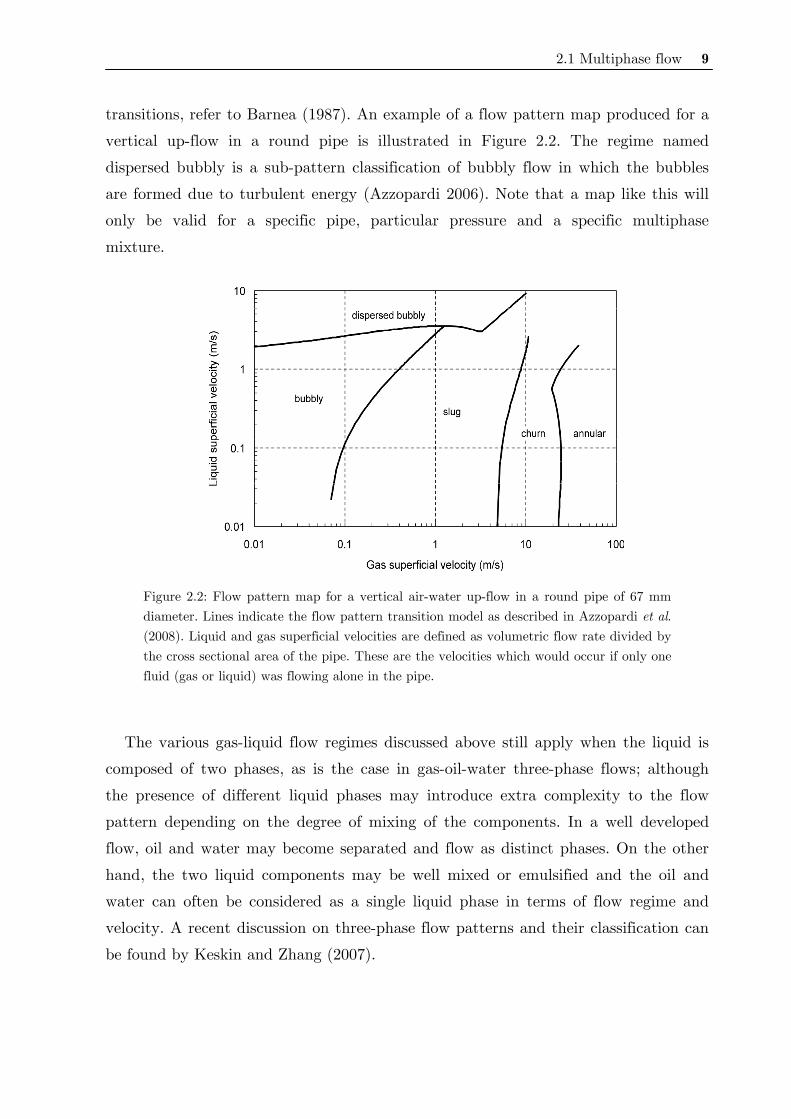
transitions, refer to Barnea (1987). An example of a flow pattern map produced for a
vertical up-flow in a round pipe is illustrated in Figure 2.2. The regime named
dispersed bubbly is a sub-pattern classification of bubbly flow in which the bubbles
are formed due to turbulent energy (Azzopardi 2006). Note that a map like this will
only be valid for a specific pipe, particular pressure and a specific multiphase
mixture.
Figure 2.2: Flow pattern map for a vertical air-water up-flow in a round pipe of 67 mm diameter. Lines indicate the flow pattern transition model as described in Azzopardi et al. (2008). Liquid and gas superficial velocities are defined as volumetric flow rate divided by the cross sectional area of the pipe. These are the velocities which would occur if only one fluid (gas or liquid) was flowing alone in the pipe.
The various gas-liquid flow regimes discussed above still apply when the liquid is
composed of two phases, as is the case in gas-oil-water three-phase flows; although
the presence of different liquid phases may introduce extra complexity to the flow
pattern depending on the degree of mixing of the components. In a well developed
flow, oil and water may become separated and flow as distinct phases. On the other
hand, the two liquid components may be well mixed or emulsified and the oil and
water can often be considered as a single liquid phase in terms of flow regime and
velocity. A recent discussion on three-phase flow patterns and their classification can
be found by Keskin and Zhang (2007).
10 2 Principles of multiphase flow measurement
2.1.2 Modeling of multiphase flow
Multiphase flows are generally of complex nature due to the existence of multiple,
deformable and moving interfaces, significant discontinuities of fluid properties and
complicated flow fields near the interface. For instance, the flow conditions in a pipe
vary along its length, over its cross section, and with time. A multiphase flow is an
extremely complex three-dimensional transient problem. Furthermore, there are
serious deficiencies in modeling of turbulence flows that occur in most practical cases
(even for single phase flow). Thus, fundamental analytical predictions of multiphase
flows are not readily achievable.
It may be possible at some distant time in the future to code the partial
differential equations governing fluid flows given by the space- and time-dependent
energy, mass, and momentum balances (known as Navier-Stokes equations) for each
of the phases and to compute every detail of a multiphase flow. But the computer
power and speed required to do this are far beyond capability for most of the flows
that are commonly experienced. Therefore, simplifications are essential in realistic
models of multiphase flows. The most common model used is the so-called two-fluid
model (Hewitt 1999, Wörner 2003, Crowe 2006). It is based on the premise that is
sufficient to describe each phase as a continuum occupying some part of the domain
space (e.g. pipe). Here, effective conservation equations (of mass, momentum and
energy) are developed for the two phases, including interaction terms between the
phases. These equations are then solved either theoretically or computationally. By
averaging terms in the equations over time, space, or other appropriate variables, the
two-fluid model may be reduced to more manageable forms, such as the time-
averaged one-dimensional model which is perhaps the most important and common
method developed for analyzing two-phase pressure drop and heat transfer (Ghajar
2005). Other frequently used models are the homogeneous and drift-flux models
(Hewitt 1999).
In recent years, the progressively increasing computer power has fostered the
development and application of flow simulation codes, commonly known as
computational fluid dynamics (CFD). A complete description of multiphase flow,
specifying the phase present and its velocity at each point in the flow and for a given
simulation time, is the approach used in CFD. Of course, space and time variables
are discretized in order to be numerically solved. Furthermore, the use of some model
(e.g. turbulence models) is required to reduce the computational power necessary to
predict the flow phenomena. A number of commercial CFD software packages are
2.2 State-of-the-art multiphase flow measuring techniques 11
currently available, for instance CFX (Ansys 2008), Fluent (Fluent 2008), OpenFoam
(OpenCFD 2008), and have successfully been applied for single phase flow problems.
CFD codes are becoming powerful tools in the hand of engineers who design plants
and have to predict flow-related safety and efficiency issues. Moreover, the use of
CFD simulations of multiphase flow is still in an early stage of development.
Although some workers have produced successful solutions to engineering multiphase
flow problems, the ultimate accuracy and the general applicability of CFD
simulations depend intrinsically on the empirical relationships and simplifications
used in codes to model multiphase flow. As a result, CFD code validation has more
and more risen to a key issue equally important to code development. It is obvious
that successful code validation is a main quality criterion for CFD codes and only
sufficiently validated code can be admitted to safety-related predictions, for instance
in nuclear reactor safety. CFD code validation requires small and medium scale
multiphase flow experiments with accurate, multi-dimensional and non- or minimal
intrusive measurement techniques for different physical parameters, such as phase
fraction distributions, temperature fields, pressure fields, velocity fields, and
concentration fields. Also therefore, multiphase flow measurement techniques have
got a strong impulse in recent years.
2.2 State-of-the-art multiphase flow measuring techniques
Online visualization and quantitative parameter assessment of multiphase flows are
highly desirable in many research and industrial application areas, for instance as
control and monitoring aid of industrial processes or as source of data for the
validation of models and simulations. Because of this high interest many efforts have
been made to develop measuring techniques to measure and image multiphase flows.
In addition to the already known problems encountered in any measuring method
for single phase flows - amply described, for instance, in Baker (2000), further
difficulties appear when attempting to measure quantities in multiphase mixtures.
One of these difficulties is related to the presence of two or more phases which of
course leads to the need for differentiation between the phases. For transient flow,
such differentiation must occur at high temporal resolution due to the unsteady
nature of the flow, i.e. a high data acquisition rate is required. Others difficulties
arrive from the conditions of flow confinement, such as opaque metallic walls, or
complex test section geometries. Such constrains may limit the use of some measuring
12 2 Principles of multiphase flow measurement
principles. Moreover, the robustness of sensors is an import issue for some industrial
applications where harsh environmental conditions occur, i.e. high pressure, high
temperature and/or the presence of aggressive media.
Despite these difficulties, advances in instrumentation technology and signal
processing techniques have led to a rapid proliferation of available experimental
methods for measurement of practical or fundamental parameters in multiphase flows
with a fair degree of accuracy. The purpose of this section is to present the principles
of a few state-of-the-art measuring techniques mainly focused on void fraction and
phase distribution measurement in gas-liquid flows. Good reviews in this field are
given by Boyer et al. (2002), Bertola (2003) and Hammer et al. (2006).
For reviews covering a broader spectrum following references are indicated.
• An overview on multiphase flow measurement in general can be gained from
the review Oddie et al. (2004).
• For further details of measurement techniques specifically intended for
gas-solid flow, see Werther (1999),
for liquid-solid (or slurry) flow, see Mishra et al. (1997), and
for liquid-liquid flow, see Jana et al. (2007).
• Furthermore, two review papers have mainly focused on the discussion of
experimental techniques for CFD validations (Tayebi et al. 2001, Prasser
2008).
2.2.1 Phase fraction measurement
The phase fraction for gas-liquid flows is commonly known as the void fraction for
the gas phase and the liquid hold-up for the liquid phase. Both quantities are
interchangeable with help of the continuity equation which requires the sum of
gaseous and liquid phase fraction to equal unity. Thus, in the following the term void
fraction will be preferably used to indicate the phase fraction.
Void fraction is a dimensionless quantity indicating the fraction of a geometric or
temporal domain occupied by the gaseous phase. It is one of the most import
parameters used to characterize multiphase flows. It is the key physical value for
determining numerous other important parameters, such as mixture density and
viscosity, for obtaining the relative averaged velocity of the phases, and is of

2.2 State-of-the-art multiphase flow measuring techniques 13
fundamental importance in models for predicting flow pattern transitions, heat
transfer and pressure drop (Azzopardi 2006, Crowe 2006).
Phase fractions may be mathematically described by the introduction of a phase
indicator (or density) function Pk which is a binary function and represents the
presence or absence of phase k at a given position x and given time t, hence
( )1 if phase
,0 if phase k
kP t
k
⎧ ∈⎪⎪= ⎨⎪ ∉⎪⎩
xx
x. (2.1)
By averaging the gas indicator function PG over different spatial or temporal domains
one can obtain different definitions for the void fraction, e.g. local, radial, cross-
sectional and volumetric (Delhaye et al. 1981, Bertola 2003).
Void fraction measurement techniques are based on various principles. Usually,
instruments are sensitive to some physical property which is different for each phase,
such as density or electrical conductivity. In this section, measuring techniques for
local and cross-sectional measurements are depicted. In addition, a brief introduction
to the challenging field of three-phase flow metering in the oil industry is given.
a) Local measurement
Local void fraction is typically measured using a miniature needle-shaped probe,
which determines the actual phase present at the probe tip. Needle probes are
designed to pierce bubbles and droplets. In this way, they determine the phase
indicator function (2.1) at a given point x. From the measured gas indicator function
PG, the local time-averaged void fraction is defined as
( ) ( )G1lim ,
TT
P t dtT
α→∞
= ∫x x . (2.2)
For a sufficiently long measurement time T (2.2) can be approximated by
( ) G G
G L
T TT T T
α = =+
x , (2.3)
where TG and TL denote the cumulated residence-time of the gas and liquid phases
within the time interval T. By moving the probe in different positions, a mapping of
the void fraction distribution in a given area or volume can be achieved, though it is
sometimes a cumbersome practice.
14 2 Principles of multiphase flow measurement
Different measuring principles based on conductance, capacitance, optical,
temperature or electrochemical measurements have been applied to the differentiation
of phases. Excellent reviews are found in Cartellier and Achard (1990) and Jones and
Delhaye (1976). However, the most common are electrical and optical needle probes.
In the case of optical probes, a light beam is guided along the probe, usually by
means of an optical fiber, to its tip. Depending on the phase present at probe tip, the
light is transmitted trough the medium or reflected back. A photodetector at the
other end of the fiber converts the intensity of the reflected light into a voltage signal
thus being an indicator for the phase.
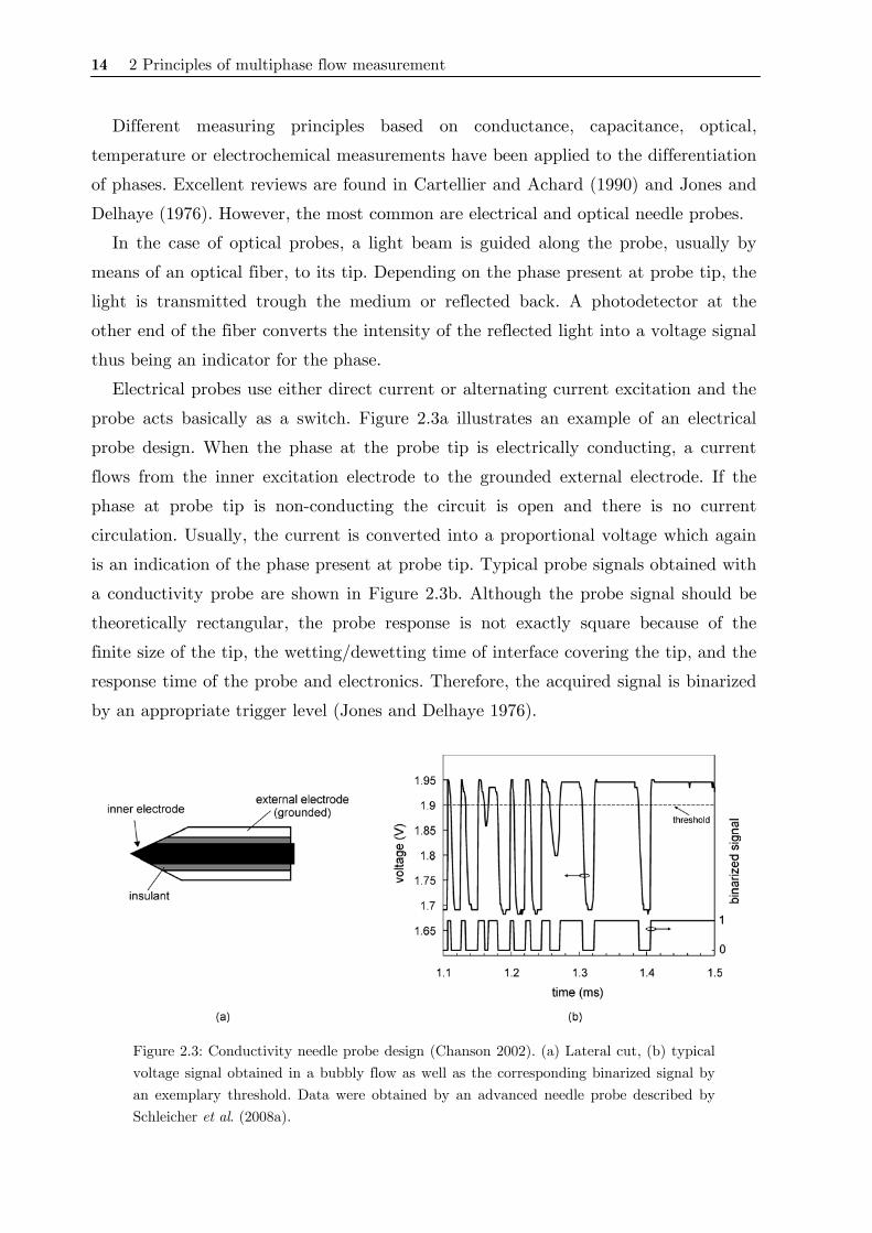
Electrical probes use either direct current or alternating current excitation and the
probe acts basically as a switch. Figure 2.3a illustrates an example of an electrical
probe design. When the phase at the probe tip is electrically conducting, a current
flows from the inner excitation electrode to the grounded external electrode. If the
phase at probe tip is non-conducting the circuit is open and there is no current
circulation. Usually, the current is converted into a proportional voltage which again
is an indication of the phase present at probe tip. Typical probe signals obtained with
a conductivity probe are shown in Figure 2.3b. Although the probe signal should be
theoretically rectangular, the probe response is not exactly square because of the
finite size of the tip, the wetting/dewetting time of interface covering the tip, and the
response time of the probe and electronics. Therefore, the acquired signal is binarized
by an appropriate trigger level (Jones and Delhaye 1976).
Figure 2.3: Conductivity needle probe design (Chanson 2002). (a) Lateral cut, (b) typical voltage signal obtained in a bubbly flow as well as the corresponding binarized signal by an exemplary threshold. Data were obtained by an advanced needle probe described by Schleicher et al. (2008a).

2.2 State-of-the-art multiphase flow measuring techniques 15
Choosing the one or other physical principle behind the needle probe
measurements is of course a matter of the type of substances to be investigated. For
instance, the first requirement to be met when using conductivity or optical probe in
two-phase flow is that one phase has a significantly different electrical conductivity or
refraction index, respectively.
Needle probes are used as single-tip or double-tip designs, depending on the kind of
data expected: single-tip probes lead to gas fraction, and bubbling frequency; double-
tip probes allow measurements of bubble velocity, mean bubble chord length and
time-average local interfacial area (Cartellier and Achard 1990).
Some researchers proposed multiple point probes, for instance a four tip probe
(Kim and Ishii 2001). Such probes can determine other components of dispersed
phase velocity regardless of bubble shape, diameter and direction. However, the
probes rapidly become bulky and so hydrodynamic interaction between bubbles and
the probe can no longer be neglected. In addition, the data analysis to extract
physical quantities is much more complex than for single-tips probes.
b) Cross-sectional measurement
The cross-sectional averaged void fraction αc-s yields from averaging the phase
indicator function (2.1) over the cross-sectional area A of a pipe or vessel at a given
time
( ) ( ) Gc-s G
G L
1 ,A
At P t daA A A
α = =+∫ x , (2.4)
where AG and AL denote the cumulated cross-sectional areas occupied by the gas and
liquid phases, respectively, within the cross section considered. It is typically
measured by means of radiation attenuation or electrical impedance techniques which
are described below.
Figure 2.4: Two schemas for the measurement of cross-sectional void fraction by radiation attenuation techniques. (a) One-shot technique, (b) multibeam densitometer.
16 2 Principles of multiphase flow measurement
Usually setup of radiation attenuation techniques consist of a radioactive source
(commonly γ-ray or x-ray but also neutrons) and a radiation detector, placed so that
the beam passes trough the flow and is monitored on the opposite side of the
multiphase mixture (Figure 2.4). For a homogeneous medium the radiation
attenuation of a collimated, mono-energetic beam follows the exponential law
( )0 expI I dμ= − , (2.5)
where I0 is the intensity of incident radiation, I is the intensity of transmitted
radiation, μ is the absorption coefficient of medium and d is the distance the beam
travels through the medium. For the measurement of cross-sectional void fraction the
narrow beam must be replaced by a linear source (a radiation sheet, Figure 2.4). This
is called one-shot technique. However, for this configuration the simple relationship
(2.5) does not hold, because absorption depends on both flow pattern and pipe
geometry, so that calibration measurements with mockup setups that simulate the
different flow regimes and void fractions are necessary. Another way to obtain αc-s is
to employ a multibeam densitometer. An exemplary setup with only three beams is
shown in Figure 2.4. The beams are attenuated according to (2.5) and the
measurement of the attenuation of each beam can be used to determine the cross-
sectional void fraction by the numerical integration (Delhaye et al. 1981).
Typical commonly used radioactive sources of gamma radiation include isotopes of
americium, cesium or cobalt. Radiation is generally detected by means of a
scintillator coupled to a photodetector. The scintillator absorbs radiation and emits
visible light by fluorescence (Johansen 2005).
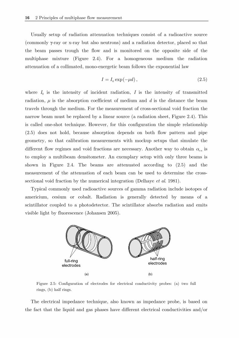
Figure 2.5: Configuration of electrodes for electrical conductivity probes: (a) two full rings, (b) half rings.
The electrical impedance technique, also known as impedance probe, is based on
the fact that the liquid and gas phases have different electrical conductivities and/or
2.2 State-of-the-art multiphase flow measuring techniques 17
relative permittivities. Impedance probes offer high frequency response, low cost, and
relative ease of construction.
By placing electrodes at the perimeter of a pipe and measuring the impedance
across the electrodes, the void fraction of the pipe may be deduced. As shown by
Ceccio and George (1996) in their extensive review analysis on impedance techniques,
there are many different possibilities to arrange a system of electrodes for void
fraction measurement purposes. Furthermore, the impedance technique has been
almost exclusively implemented in two categories depending on the type of
instrumentation used and liquid material to be investigated: electrical conductivity
and capacitance probes.
With reference to the conductivity probes, flush-mounted ring electrodes were
successfully employed first by Asali et al. (1985), and then by Andreussi et al. (1988),
Tsochatzidis et al. (1992), Fossa (1998), among others. A typical arrangement is
represented by two metallic rings annealed in the pipe inner wall, as shown in Figure
2.5a. Ma et al. (1991) and later Costigan and Whalley (1997) developed a probe with
other electrode configuration which has been also successfully employed for the
investigation of two-phase flows. It is constituted by a pair of measuring half-rings
facing one another with two guard electrodes (again half-rings) maintained at the
potential of the corresponding measuring electrodes (Figure 2.5b).
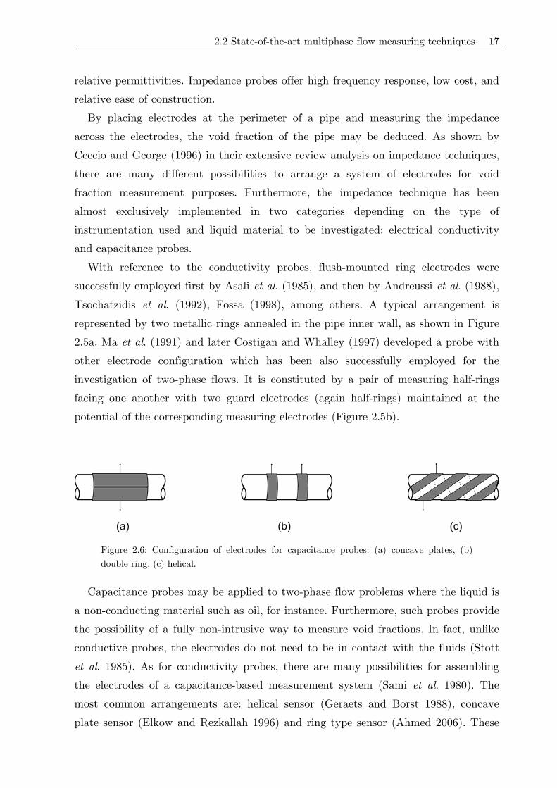
Figure 2.6: Configuration of electrodes for capacitance probes: (a) concave plates, (b) double ring, (c) helical.
Capacitance probes may be applied to two-phase flow problems where the liquid is
a non-conducting material such as oil, for instance. Furthermore, such probes provide
the possibility of a fully non-intrusive way to measure void fractions. In fact, unlike
conductive probes, the electrodes do not need to be in contact with the fluids (Stott
et al. 1985). As for conductivity probes, there are many possibilities for assembling
the electrodes of a capacitance-based measurement system (Sami et al. 1980). The
most common arrangements are: helical sensor (Geraets and Borst 1988), concave
plate sensor (Elkow and Rezkallah 1996) and ring type sensor (Ahmed 2006). These
18 2 Principles of multiphase flow measurement
electrode configurations are depicted in Figure 2.6. It is common that the capacitance
of those setups is in the range of 0.1 to 10 pF. Thus, proper shielding against stray
capacitance and a good signal-to-noise ratio are extremely important for a correct
void fraction measurement. Articles by Huang et al. (1988, 1989) have reviewed
electrode guard methods and capacitance measurement techniques.
Combination of conductive and capacitive measurements has been also reported in
the literature, but this practice is less common. The measurement of the complex
value of impedance was described for three component fraction measurement
(Dykesteen et al. 1985) and for water content measurement in oil-water emulsions
(García-Golding et al. 1995).
c) Multiphase flow metering in the oil industry
Three-phase gas-oil-water flows are common in the oil industry. Most of the gas and
oil reservoirs naturally contain water or due to the pressure decrease with production,
the natural pressure of an oil reservoir is maintained by injecting water. Therefore,
water is produced along with oil and gas which results in a three-phase gas-oil-water
flow in wellbore and surface gathering systems. Three-phase flows thus occur in the
wells, in the flow lines connecting the wells to the platform and in the risers
conducting the fluid from the flow lines to the top of the platform (Hewitt 2005).
Under the multiphase flow circumstances, the following parameters are required to
compute flow rates of each phase: (i) the cross-sectional phase fraction and (ii) the
axial velocity of each phase. The volumetric flow rate Qx of a given phase x is
determined by the product of phase velocity Ux and area of the pipe occupied by the
respective phase Ax
x x xQ A U= ⋅ (2.6)
Since Ax may be calculated from the phase fraction x xA A α= ⋅ , where A is the pipe
area, basically six variables must be estimated in the general multiphase
measurement problem, i.e. three phase fractions and three phase velocities (Letton et
al. 1997):
( )T O G W O O G G W WQ Q Q Q A U U Uα α α= + + = ⋅ + ⋅ + ⋅ , (2.7)
where the subscripts O, G, and W denote oil, gas and water phases in a three-phase
flow, respectively.

2.2 State-of-the-art multiphase flow measuring techniques 19
In this way, making measurements in such three-phase flows presents special
difficulties. A distinction needs to be made between the gas and liquid phases, and
also between the primary and secondary liquid components. Basically two strategies
have been used in multiphase flow meters in the gas and oil industry: phase
separation meters or in-line meters. For a review in that field, Corneliussen et al.
(2005), and the review in Baker (2000, chapter 14) are indicated.
Phase separation meters, as the name already suggests, are characterized by the
fact that the phases are separated before measurement. The three phases are then
measured individually using some single-phase measuring technique. With the space
on a production platform becoming more expensive, and the development of subsea
production systems increasing, the use of conventional offshore separators is becoming
less desirable. Therefore, the growth in research and development of in-line
multiphase flow metering systems has been exponential since the early 1980s (Falcone
et al. 2002).
Today there is a variety of in-line multiphase flow meters installed onshore and
offshore and other being developed which use different sensing techniques and models
to calculate multiphase flow rates via (2.7). For the measurement of phase fractions,
current systems are based on dual energy gamma ray method or the combination of
two of the following techniques: mono-energetic gamma ray absorption,
resistance/capacitance measurements or microwave sensors (Babelli 2002, Falcone et
al. 2002, Yeung 2007). Recently, a dual energy x-ray tomograph has been presented
by Hu et al. (2005) for time-resolved phase fraction distribution measurement which
has been used only for research purposes yet. Phase velocities are usually measured
by cross-correlation techniques from signals of two axially spaced sensors. With an
alternative approach, some other flow meters firstly homogenize the flow assuring all
phases are well-mixed and the assumption that all three phases flow with equal
velocity (Uo = Ug = Uw = U) may be applied. The mixture velocity is then
determined by a conventional venturi meter or a positive displacement meter.
Varying level of accuracy requirements exists in multiphase flow measurement
depending on how the information will be utilized, for instance, for fiscal or
monitoring purposes. Although many alternative metering systems have been
developed and tested, none can be referred to as universally accurate and/or
applicable. The market potential is huge. Yeung (2007) estimates that only 0.2% of
current oil wells are instrumented with multiphase flow meters. Thus, there are many
20 2 Principles of multiphase flow measurement
opportunities; and the search for new technologies and innovative solutions for this
challenging field still persists.
2.2.2 Tomographic flow imaging
Tomographic multiphase flow imaging, more commonly called process tomography or
industrial process tomography, finds many applications in the imaging and
measurement of industrial processes. A tomographic image is a two-dimensional
representation of a slice through an object. The use of various tomographic methods
is widespread in diagnostic medicine (Kak and Slaney 1988) and several imaging
modalities originally developed for medical imaging are now being adapted to
industrial process imaging. The use of tomographic imaging for the investigation of
multiphase flows has been reported in a few exhaustive review papers (Dyakowski
1996, Chaouki et al. 1997, Williams and Jia 2003, Prasser 2008) and books (Williams
and Beck 1995, McCann and Scott 2005).
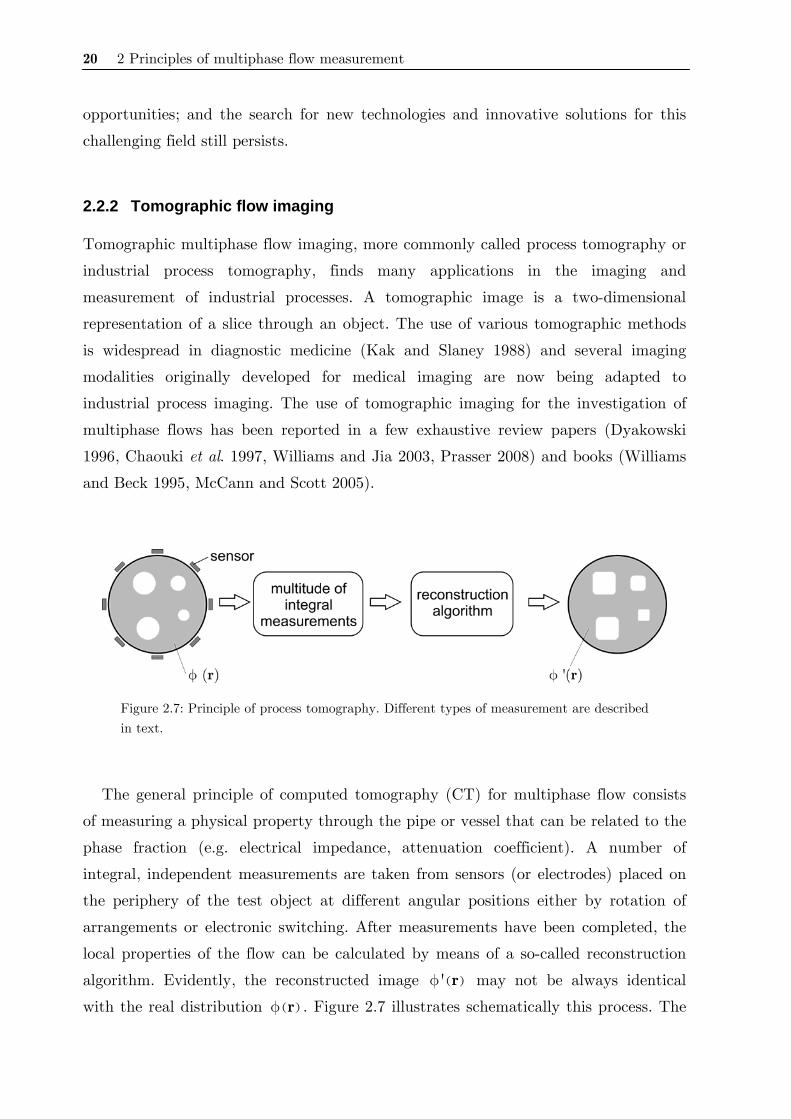
Figure 2.7: Principle of process tomography. Different types of measurement are described in text.
The general principle of computed tomography (CT) for multiphase flow consists
of measuring a physical property through the pipe or vessel that can be related to the
phase fraction (e.g. electrical impedance, attenuation coefficient). A number of
integral, independent measurements are taken from sensors (or electrodes) placed on
the periphery of the test object at different angular positions either by rotation of
arrangements or electronic switching. After measurements have been completed, the
local properties of the flow can be calculated by means of a so-called reconstruction
algorithm. Evidently, the reconstructed image ( )'φ r may not be always identical
with the real distribution ( )φ r . Figure 2.7 illustrates schematically this process. The
2.2 State-of-the-art multiphase flow measuring techniques 21
image reconstruction in tomography implies solving an inverse problem, i.e. obtaining
the spatial distribution of the imaged parameter from a plurality of measurements
and the known geometry of the problem. A conventional computer is often used for
off-line image reconstruction. However, for real-time reconstruction parallel
computing systems may be applied. There are many types of tomography systems
based on different sensing techniques such as electrical, ultrasound, radiation. A short
description of current most common tomographic technique for multiphase flow
measurement is given in the following.
a) X-ray, γ-ray and neutron tomography
X-ray, γ-ray and neutron tomography can be seen as an evolution of the
densitometry method for cross-sectional void fraction measurement as described in
section 2.2.1b). These modalities are based on the attenuation of radiation by matter.
Since gas and liquid present different attenuation characteristics for the radiation,
images of void fraction distributions may be obtained. The set of projections needed
for the reconstruction of the images are generated either by rotating source and
detectors around the pipe or by the use of multiple source and detectors (Johansen
2005). The use of x-ray tomography for void fraction measurements was described,
for instance, by Hervieu et al. 2002 and Heindel et al. (2008), while use of gamma ray
tomography was reported by Kumar et al. (1995), Hampel et al. (2007), among
others. All the above-mentioned techniques yield time-averaged rather than
instantaneous phase distribution images due to the use of mechanically rotating
parts. The time resolution of such systems is limited to a few images per second.
Attempts to increase time resolution have been reported by Johansen et al. (1996)
who describe a γ-ray tomography system operated by five gamma sources in parallel
capable to generate 100 fps, by Hori et al. (1998) who introduced a multitube x-ray
scanner which achieve 2 000 fps and recently by Bieberle et al. (2007) who used an
electron beam to generate a fast moving x-ray spot and reached 10 000 fps. These
approaches allow the study of dynamically changing phase distributions. However,
such solutions are still comparatively complex and cost-intensive.
Neutrons have some advantages in terms of their attenuation in matter in
comparison to photons. For example, organic materials or water are clearly visible in
neutron radiographs because of their high hydrogen content, while many structural
materials such as aluminium or steel are nearly transparent. Nevertheless, neutron
22 2 Principles of multiphase flow measurement
tomography requires complex, expensive and heavy equipment for the generation of
neutrons, and therefore its use for the investigation of multiphase flows has been
limited in the past (Hussein et al. 1986).
b) Magnetic resonant imaging
Magnetic resonant imaging (MRI) is widely used in medical diagnostics, which is
based on the paramagnetic properties of the nuclei. MRI scanners use the
phenomenon of nuclear magnetic resonance of hydrogen nuclei in conjunction with
radio frequency (rf) and magnetic gradient pulses to map the object under
investigation (Mantle and Sederman 2003). Basically, MRI detects the concentration
of hydrogen atoms, thus liquid water presents excellent contrast. MRI is able not
only to determine the density of nuclei but also the velocity in case of moving
objects. Mantle and Sederman (2003) and Hall (2005) reported some flow applications
of MRI in their reviews. Some limitations of MRI are the necessity of non-magnetic,
non-conducting pipes to allow the measurements, the rather low imaging frequency
and the relatively high hardware cost. A special MRI technique called Echo-planar
Imaging can achieve up to 140 frame per second and it was used to investigate slug
flow (Reyes Jr. et al. 1998). However, this technique needs even more costly hardware
than conventional MRI to achieve such a frame rate.
c) Positron emission tomography
Positron emission tomography (PET) is based on the use of a γ-ray emitting
radioisotope as a flow tracer. External detectors are used to measure the number of
rays emerging from the system which provides the information needed to reconstruct
the tracer distribution by the standard tomographic approach. In a multiphase flow,
one of the phases can be labeled and its behavior analyzed (Parker and McNeil 1996).
However, the acquisition time of a PET system lies in the order of minutes and is
thus too slow for rapidly evolving flows. An alternative method is the positron
emission particle tracking (PEPT) which involves introducing a single labeled tracer
particle in the process which has its trajectory tracked by using advanced algorithms
(Parker et al. 1993). The overall system time response is in the range of milliseconds
and a particle moving at speeds about 1 m/s was reliably followed.

2.2 State-of-the-art multiphase flow measuring techniques 23
d) Optical tomography
Optical tomography uses low energy electromagnetic radiation, either of the infrared,
visible or ultraviolet wavelength range, to measure extinction profiles from an object
and subsequently reconstruct the data by means of CT algorithms. A few researchers
have reported on optical tomography for the investigation of single phase and
multiphase flows (Rzasa and Plaskowski 2003, Ruzairi and Chan 2004, Schleicher et
al. 2008b). The common characteristic of these systems is the use of low-cost light
emitters and detectors. Another example of optical tomography applied to process
investigation is described by Carey et al. (2000) and Hindle et al. (2001), who
performed chemical species imaging by exploiting specific substance absorption at
near-infrared band. Optical tomographs may reach very high temporal resolution of a
few thousand frames/s. Nevertheless, regarding gas-liquid flows, optical systems can
only be successfully employed to flows with low void fraction (typically up to 10%)
due to the fact that the flow becomes opaque for light at high voidage. Optical
systems also need transparent walls and transparent liquids to be able to investigate
the flow.
e) Ultrasound tomography
Tomography based on ultrasonic waves has also been applied to investigate
multiphase flows (Hoyle 1996). An ultrasonic system detects changes in the acoustic
impedance properties between objects. Gas-liquid flow exhibits a marked acoustic
impedance difference between gas and liquid interfaces. In ultrasound tomography
multiple ultrasonic transducers are mounted around the pipe. Basically, reflection
mode (Yang M. et al. 1999) and transmission mode (Rahiman et al. 2006, Supardan
et al. 2007) measurements can be applied, in which the reflected or transmitted
ultrasonic waves are evaluated, respectively, along with suitable reconstruction
procedure. Frame rates obtained are in the range of a few hundred images per second.
One advantage of ultrasound tomography is the possibility to image flows inside
opaque objects. However, the limitation regarding low void fractions is similar as for
optical systems.
f) Electrical tomography
An important field in process tomography is the one concerned with electrical
impedance tomography (EIT) which exploits the interaction of electrical fields with
matter. The main task of EIT is to determine conductivity or permittivity
24 2 Principles of multiphase flow measurement
distributions which are linked to phase distributions in a multiphase flow. Thus, EIT
is also referred to electrical resistance tomography (ERT) or electrical capacitance
tomography (ECT) depending on the modality. Some researchers have erroneously
used the term EIT as synonym to ERT. However EIT should be used only when both
resistance and capacitance are measured (called dual-modality), as described by
Marashdeh et al. (2007) and Cao et al. (2007).
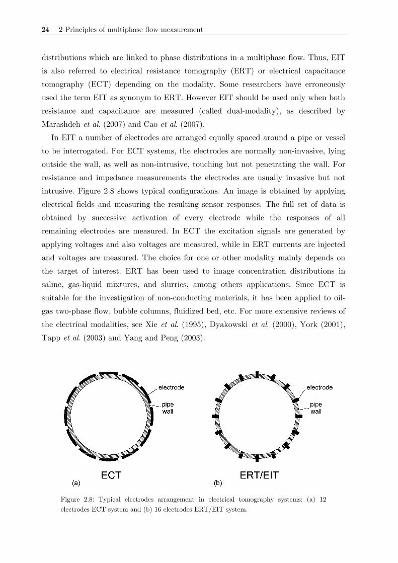
In EIT a number of electrodes are arranged equally spaced around a pipe or vessel
to be interrogated. For ECT systems, the electrodes are normally non-invasive, lying
outside the wall, as well as non-intrusive, touching but not penetrating the wall. For
resistance and impedance measurements the electrodes are usually invasive but not
intrusive. Figure 2.8 shows typical configurations. An image is obtained by applying
electrical fields and measuring the resulting sensor responses. The full set of data is
obtained by successive activation of every electrode while the responses of all
remaining electrodes are measured. In ECT the excitation signals are generated by
applying voltages and also voltages are measured, while in ERT currents are injected
and voltages are measured. The choice for one or other modality mainly depends on
the target of interest. ERT has been used to image concentration distributions in
saline, gas-liquid mixtures, and slurries, among others applications. Since ECT is
suitable for the investigation of non-conducting materials, it has been applied to oil-
gas two-phase flow, bubble columns, fluidized bed, etc. For more extensive reviews of
the electrical modalities, see Xie et al. (1995), Dyakowski et al. (2000), York (2001),
Tapp et al. (2003) and Yang and Peng (2003).
Figure 2.8: Typical electrodes arrangement in electrical tomography systems: (a) 12 electrodes ECT system and (b) 16 electrodes ERT/EIT system.
2.2 State-of-the-art multiphase flow measuring techniques 25
EIT systems are relatively fast (up to 1 000 images per second), low cost and
simple to operate. The main disadvantage of EIT is its moderate spatial resolution of
the resultant image. The measured electrical signals are a non-linear function of
phase fractions and flow configuration and unlike x-ray or γ-rays, electrical fields
cannot be confined to a narrow path between a transmitter and receiver. This is
called the soft-field property of electrical tomography.
A third electrical modality, electromagnetic tomography (EMT) or magnetic
inductance tomography has been reported which is based on mutual inductance
measurements. EMT is suitable for imaging highly conducting or magnetic materials,
such as metals and minerals (Peyton et al. 1996).
2.2.3 Wire-mesh sensor
Wire-mesh sensors are flow imaging devices and allow the investigation of multiphase
flows with high spatial and temporal resolution. Although they could not be
considered belonging to classical tomographic technique, because their working
principle is based on intrusive electrodes to generate the images, it has been accepted
as an alternative technique to the tomography systems previously described. This
type of sensor was introduced about ten years ago by Prasser et al. (1998) at FZD
and since then it has been successfully employed by a number of researchers to
investigate different single phase and two-phase flow phenomena. An overview over
the capabilities of wire-mesh sensors was recently summarized by Prasser (2008).
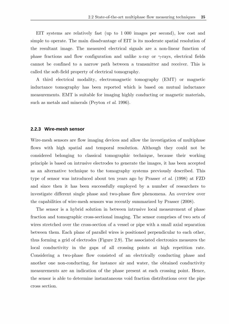
The sensor is a hybrid solution in between intrusive local measurement of phase
fraction and tomographic cross-sectional imaging. The sensor comprises of two sets of
wires stretched over the cross-section of a vessel or pipe with a small axial separation
between them. Each plane of parallel wires is positioned perpendicular to each other,
thus forming a grid of electrodes (Figure 2.9). The associated electronics measures the
local conductivity in the gaps of all crossing points at high repetition rate.
Considering a two-phase flow consisted of an electrically conducting phase and
another one non-conducting, for instance air and water, the obtained conductivity
measurements are an indication of the phase present at each crossing point. Hence,
the sensor is able to determine instantaneous void fraction distributions over the pipe
cross section.
26 2 Principles of multiphase flow measurement
Figure 2.9: (a) schematic representation of a wire-mesh sensor; (b) photograph of a typical sensor developed at FZD.
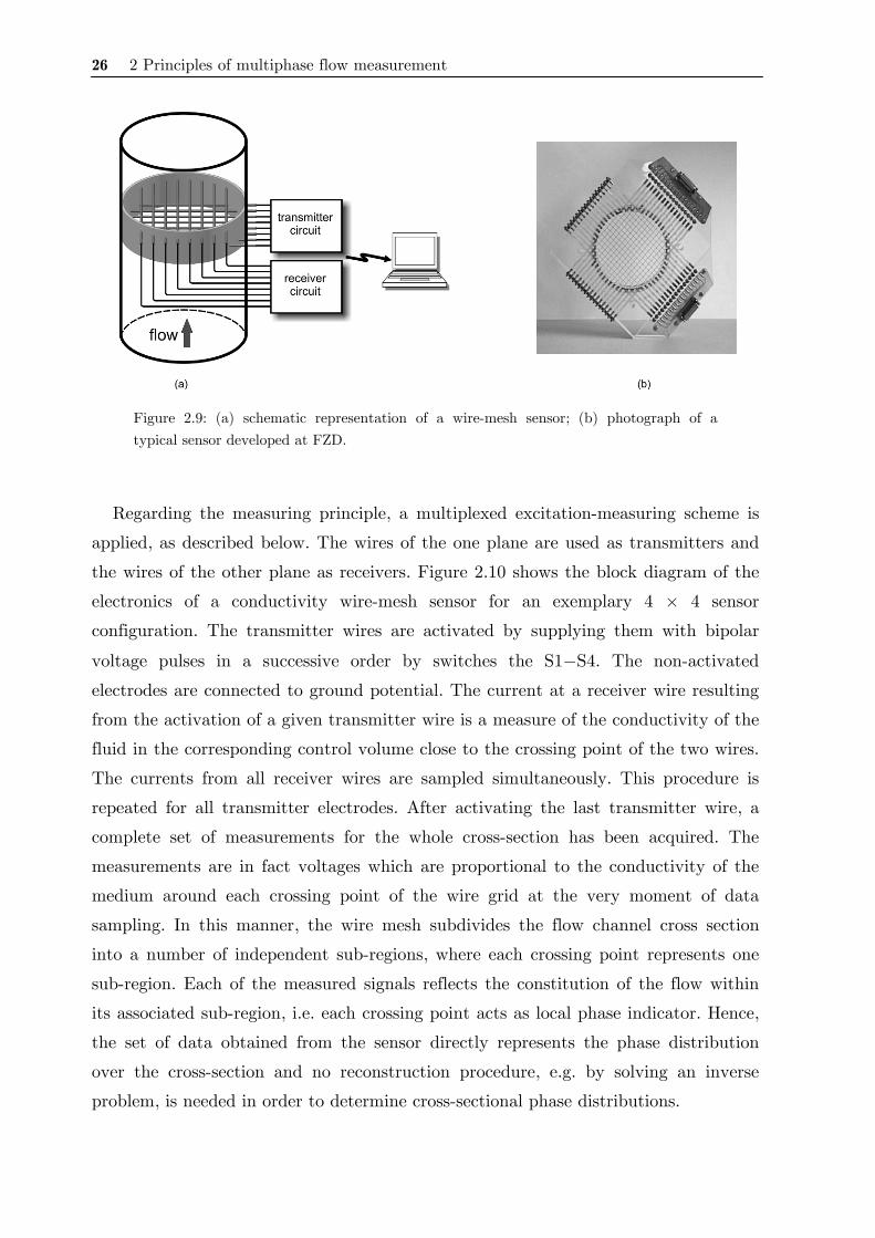
Regarding the measuring principle, a multiplexed excitation-measuring scheme is
applied, as described below. The wires of the one plane are used as transmitters and
the wires of the other plane as receivers. Figure 2.10 shows the block diagram of the
electronics of a conductivity wire-mesh sensor for an exemplary 4 × 4 sensor
configuration. The transmitter wires are activated by supplying them with bipolar
voltage pulses in a successive order by switches the S1−S4. The non-activated
electrodes are connected to ground potential. The current at a receiver wire resulting
from the activation of a given transmitter wire is a measure of the conductivity of the
fluid in the corresponding control volume close to the crossing point of the two wires.
The currents from all receiver wires are sampled simultaneously. This procedure is
repeated for all transmitter electrodes. After activating the last transmitter wire, a
complete set of measurements for the whole cross-section has been acquired. The
measurements are in fact voltages which are proportional to the conductivity of the
medium around each crossing point of the wire grid at the very moment of data
sampling. In this manner, the wire mesh subdivides the flow channel cross section
into a number of independent sub-regions, where each crossing point represents one
sub-region. Each of the measured signals reflects the constitution of the flow within
its associated sub-region, i.e. each crossing point acts as local phase indicator. Hence,
the set of data obtained from the sensor directly represents the phase distribution
over the cross-section and no reconstruction procedure, e.g. by solving an inverse
problem, is needed in order to determine cross-sectional phase distributions.
2.2 State-of-the-art multiphase flow measuring techniques 27
Figure 2.10: Wire-mesh sensor electronics with a 4 × 4 sensor configuration (Prasser et al. 1998).
From the first publication (Prasser et al. 1998) the technology of wire-mesh sensors
has steadily been developed towards increasing frame rate (Prasser et al. 2002b),
bubble size measurement (Prasser et al. 2001), gas phase velocity measurement
(Manera et al. 2006), measurement at elevated pressures (Pietruske and Prasser
2007). In the scope of research work wire mesh sensors have extensively been used in
the following fields: steam-water pipe flow (Prasser et al. 2007), mixing scenarios in
pressurized water reactor models (Prasser et al. 2003), water hammers in pipes
(Dudlik et al. 2002), and transient boiling (Manera et al. 2006). Today sensors can be
devised with up to 64 × 64 wires, wire diameters down to 0.05 mm, in diversity of
different cross-section geometries and operating parameters. High-pressure wire-mesh
sensors can be employed for temperatures and pressures up to 286 °C and 7 MPa,
respectively (Pietruske and Prasser 2007). Associated electronics for signal generation
and data acquisition achieves a maximum temporal resolution of 10 000 frames per
second (Prasser et al. 2002b).
The intrusiveness effect of wire-mesh sensors has been investigated by high-speed
camera measurements (Prasser et al. 2001, Wangjiraniran et al. 2003) and by
comparison with a fast x-ray tomography system (Prasser et al. 2005b). The results
have shown that the sensor yields images of an undisturbed flow. Influences of the
mesh are found only downstream from the sensor. In this way, wire-mesh sensors
offer a compromise. The disadvantage of being intrusive is in part compensated by
high temporal resolution, low cost, and simplicity when compared with other imaging
systems.
28 2 Principles of multiphase flow measurement
Another wire-mesh device was also introduced by Reinecke et al. (1996, 1998).
However, this device employs three set of wires forming an angle of 120° whereby the
conductance of each parallel wire pair is measured. In this way, three independent
projections of the flow cross section are obtained. The conductivity distribution is
interpreted as the void fraction distribution. The transformation from the measured
conductance data into the image has to be performed by applying a tomographic
image reconstruction algorithm. This is the main difference to the above described
sensor (which performs direct flow imaging) and also is the main disadvantage of this
solution. The system of equations to be solved for the image reconstruction is highly
underdetermined and must be iteratively resolved which cannot be assumed free of
artifacts and is very time consuming.
2.2.4 Other techniques
Gas-liquid flows have been also investigated by a variety of other measuring
techniques different to those discussed above. Some examples are optical and
velocimetry methods.
Optical visualization is probably the first diagnostic tool chosen when multiphase
flows are investigated. High-speed cameras are easy to operate and typically reach
frame rates of tens of kilohertz. Thus, by proper image processing algorithms, optical
visualization techniques are useful to investigate the form and behavior of bubbles
(e.g. shape, size, velocity), as well as phase boundaries in gas-liquid flows. It has been
very frequently reported in the literature (e.g. Lage and Esposito 1999, Zaruba et al.
2005). The limitations of optical techniques are obvious: only the vicinity of the wall
can be observed at high void fraction and transparent walls as well as a transparent
liquid are required.
Another classical optical technique for flow studies is the particle image
velocimetry (PIV). It is used for measuring the instantaneous flow velocity. Images of
small tracers freely flowing in the fluid under study are acquired at two or more
times by pulsing some light source (Adrian 1991). The motion of these tracers is then
a measure of the motion of the fluid, and, consequently, a whole flow field can be
estimated. Recently, PIV technique has been further developed and successfully
applied to study gas-liquid multiphase flows (Hassan 2002, Bröder and Sommerfeld
2002).
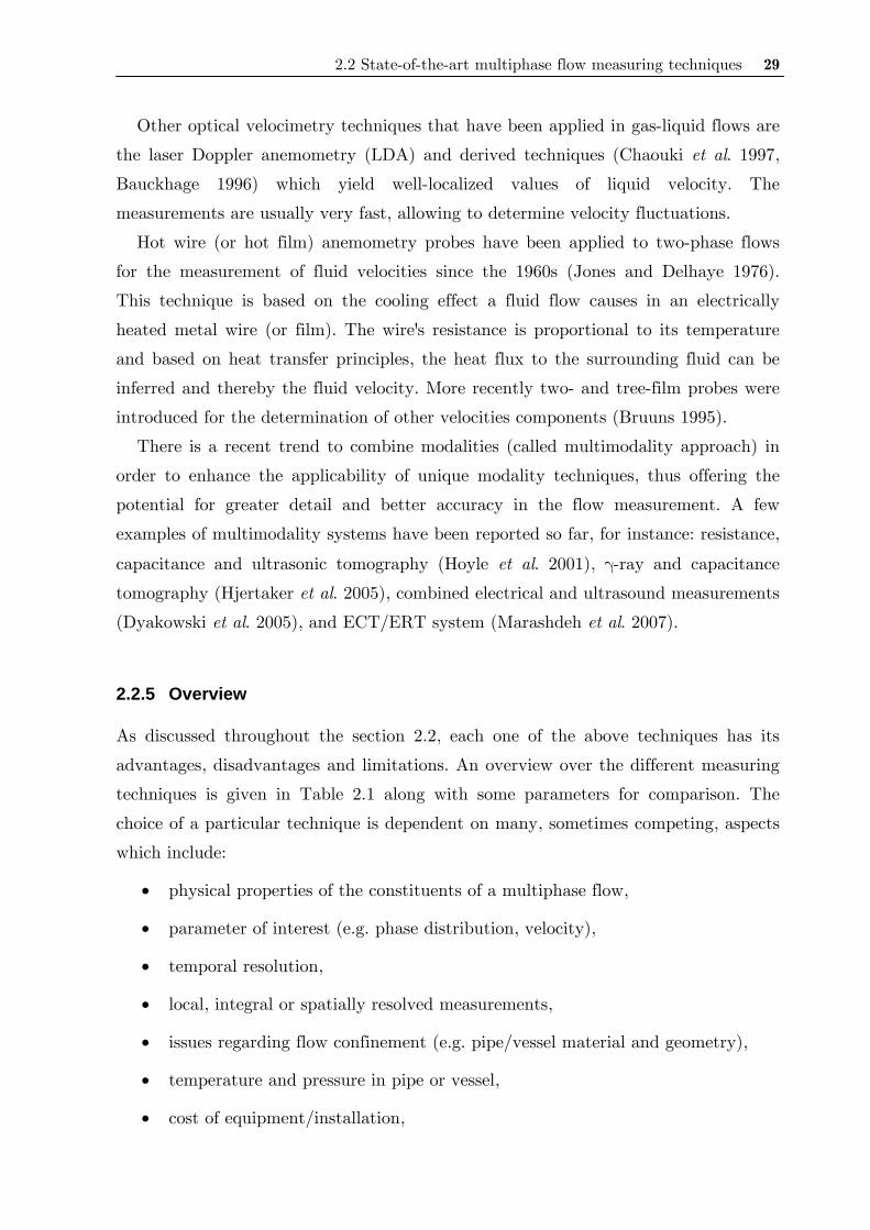
2.2 State-of-the-art multiphase flow measuring techniques 29
Other optical velocimetry techniques that have been applied in gas-liquid flows are
the laser Doppler anemometry (LDA) and derived techniques (Chaouki et al. 1997,
Bauckhage 1996) which yield well-localized values of liquid velocity. The
measurements are usually very fast, allowing to determine velocity fluctuations.
Hot wire (or hot film) anemometry probes have been applied to two-phase flows
for the measurement of fluid velocities since the 1960s (Jones and Delhaye 1976).
This technique is based on the cooling effect a fluid flow causes in an electrically
heated metal wire (or film). The wire's resistance is proportional to its temperature
and based on heat transfer principles, the heat flux to the surrounding fluid can be
inferred and thereby the fluid velocity. More recently two- and tree-film probes were
introduced for the determination of other velocities components (Bruuns 1995).
There is a recent trend to combine modalities (called multimodality approach) in
order to enhance the applicability of unique modality techniques, thus offering the
potential for greater detail and better accuracy in the flow measurement. A few
examples of multimodality systems have been reported so far, for instance: resistance,
capacitance and ultrasonic tomography (Hoyle et al. 2001), γ-ray and capacitance
tomography (Hjertaker et al. 2005), combined electrical and ultrasound measurements
(Dyakowski et al. 2005), and ECT/ERT system (Marashdeh et al. 2007).
2.2.5 Overview
As discussed throughout the section 2.2, each one of the above techniques has its
advantages, disadvantages and limitations. An overview over the different measuring
techniques is given in Table 2.1 along with some parameters for comparison. The
choice of a particular technique is dependent on many, sometimes competing, aspects
which include:
• physical properties of the constituents of a multiphase flow,
• parameter of interest (e.g. phase distribution, velocity),
• temporal resolution,
• local, integral or spatially resolved measurements,
• issues regarding flow confinement (e.g. pipe/vessel material and geometry),
• temperature and pressure in pipe or vessel,
• cost of equipment/installation,
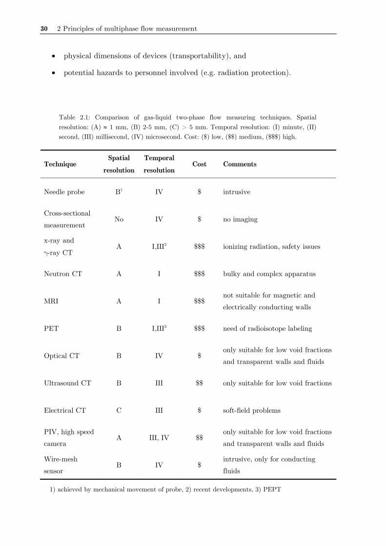
30 2 Principles of multiphase flow measurement
• physical dimensions of devices (transportability), and
• potential hazards to personnel involved (e.g. radiation protection).
Table 2.1: Comparison of gas-liquid two-phase flow measuring techniques. Spatial resolution: (A) ≈ 1 mm, (B) 2-5 mm, (C) > 5 mm. Temporal resolution: (I) minute, (II) second, (III) millisecond, (IV) microsecond. Cost: ($) low, ($$) medium, ($$$) high.
Technique Spatial
resolution
Temporal
resolution Cost Comments
Needle probe B1 IV $ intrusive
Cross-sectional
measurement No IV $ no imaging
x-ray and
γ-ray CT A I,III2 $$$ ionizing radiation, safety issues
Neutron CT A I $$$ bulky and complex apparatus
MRI A I $$$ not suitable for magnetic and
electrically conducting walls
PET B I,III3 $$$ need of radioisotope labeling
Optical CT B IV $ only suitable for low void fractions
and transparent walls and fluids
Ultrasound CT B III $$ only suitable for low void fractions
Electrical CT C III $ soft-field problems
PIV, high speed
camera A III, IV $$
only suitable for low void fractions
and transparent walls and fluids
Wire-mesh
sensor B IV $
intrusive, only for conducting
fluids
1) achieved by mechanical movement of probe, 2) recent developments, 3) PEPT
2.3 Conclusions 31
2.3 Conclusions
The study of multiphase flow phenomena is a challenging field involving
multidisciplinary knowledge disciplines. Experiments and reliable experimental
techniques are essential tools to improve the understanding about multiphase flows.
Two-phase gas-liquid flow are among the most import types of multiphase flow and
occurs extensively throughout industries, for instance, in boilers, gas and oil transport
pipelines, chemical processes.
In this chapter some essentials of gas-liquid flows were presented. Furthermore, the
principles of the major measuring techniques for the investigation of such flows were
revised and discussed. Although much progress has been made in the last years in the
development and application of flow measurement techniques, none of the proposed
techniques can claim a universal applicability or absolute accuracy for multiphase
flow measurement. Notably is need for high-speed flow measurement and imaging
required to investigate highly transient flows, which has mostly motivated the work
of this thesis. In this fashion, there is a need of innovative measuring techniques
which may fulfill the gap left open by current techniques. In this thesis, three novel
sensors based on impedance measurements are introduced. Thus, following the
current trend for multimodality techniques, a novel dual-modality
conductivity/permittivity needle probe is presented in chapter 4. A further
development of current wire-mesh sensor is described in chapter 5, where capacitance
(permittivity) measurements are used allowing the sensor to be employed in the
investigation of non-conducting fluids too. Finally, a novel non-intrusive sensor
modality for imaging fluid distributions and near-wall flows is introduced in
chapter 6.

32 2 Principles of multiphase flow measurement

33
3 Electrical impedance measurements in fluids
Impedance measurement is commonly used for circuits, components,
material or solution characterization. In this chapter the theory of
impedance and its measurement is reviewed with focus on the
impedance measurement in fluids. This chapter starts with some basic
definitions. Further it describes the electrical properties of fluids and
reviews the different impedance measuring techniques. The auto-
balancing bridge method is discussed in detail. Finally, first
impedance measurements results with a simple probe are presented.
3.1 Electrical properties of fluids
Fluids as well as matter in general may be classified according to their
electromagnetic properties. Although some fluids such as ferrofluids have appreciable
magnetic properties, most of them are non-magnetic. On the other hand, all fluids
present electrical properties, which is the focus of this section. The following
description is mainly based on the books from Dorf (2000) and Macdonald (1987).
3.1.1 Definitions: impedance and complex permittivity
In electrodynamics the impedance describes the relationship between voltage and
current for non-steady-state behavior. Mostly a sinusoidal alternating current (ac) is
considered. A voltage ( ) ( )Vcosv t V tω θ= + at angular frequency ω = 2πf is applied
to a material or circuit and the resulting electrical current ( ) ( )Icosi t I tω θ= + is
measured. The resulting impedance Z is calculated by Ohm's law in complex notation
= VZI
, (3.1)
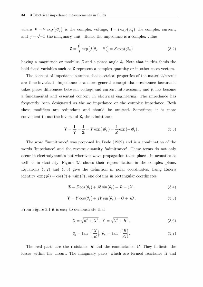
34 3 Electrical impedance measurements in fluids
where ( )VexpV jθ=V is the complex voltage, ( )IexpI jθ=I the complex current,
and 1j = − the imaginary unit. Hence the impedance is a complex value
( )( ) ( )V I Zexp expV j Z jI
θ θ θ= − =Z (3.2)
having a magnitude or modulus Z and a phase angle θZ. Note that in this thesis the
bold-faced variables such as Z represent a complex quantity or in other cases vectors.
The concept of impedance assumes that electrical properties of the material/circuit
are time-invariant. Impedance is a more general concept than resistance because it
takes phase differences between voltage and current into account, and it has become
a fundamental and essential concept in electrical engineering. The impedance has
frequently been designated as the ac impedance or the complex impedance. Both
these modifiers are redundant and should be omitted. Sometimes it is more
convenient to use the inverse of Z, the admittance
( ) ( )Y Z1 1exp expY j j
Zθ θ= = = = −IY
V Z. (3.3)
The word "immittance" was proposed by Bode (1959) and is a combination of the
words "impedance" and the reverse quantity "admittance". These terms do not only
occur in electrodynamics but wherever wave propagation takes place - in acoustics as
well as in elasticity. Figure 3.1 shows their representation in the complex plane.
Equations (3.2) and (3.3) give the definition in polar coordinates. Using Euler's
identity ( ) ( ) ( )exp cos sinj jθ θ θ= + , one obtains in rectangular coordinates
( ) ( )Z Zcos sinZ jZ R jXθ θ= + = +Z , (3.4)
( ) ( )Y Ycos sinY jY G jBθ θ= + = +Y . (3.5)
From Figure 3.1 it is easy to demonstrate that
2 2Z R X= + , 2 2Y G B= + , (3.6)
1Z tan X
Rθ − ⎛ ⎞⎟⎜= ⎟⎜ ⎟⎜⎝ ⎠,
1Y tan B
Gθ − ⎛ ⎞⎟⎜= ⎟⎜ ⎟⎜⎝ ⎠ . (3.7)
The real parts are the resistance R and the conductance G. They indicate the
losses within the circuit. The imaginary parts, which are termed reactance X and

3.1 Electrical properties of fluids 35
susceptance B, respectively, are a measure of the reactive energy stored in the circuit
during one period. In general, all these quantities are frequency-dependent.
Figure 3.1: Representation of impedance and admittance in the complex plane showing the relations between rectangular and polar coordinates. Note that the units are different for each vector.
Impedance is by definition a complex quantity and is only real when θ = 0 and
thus Z = R, that is, for purely resistive behavior. The impedance of ideal inductors
and capacitors is purely imaginary with different signs according to the phase shift of
±90° between voltage and current. A general element or network is therefore called
inductive or capacitive at a given frequency corresponding to the sign of the
imaginary part of its impedance.
The above definitions apply very well in circuit and network theory. However, a
much more common parameter used to characterize materials is the complex relative
permittivity ε . This quantity is related to the complex absolute permittivity
a 0ε= ⋅ε ε , where ε0 = 8.85 pF/m is the permittivity of free space. The relative
permittivity ε is a dimensionless quantity. In this thesis the complex relative
permittivity will be referred to as complex permittivity, denoted by ε , only. As its
name indicates it is a complex quantity
' ''jε ε= − ⋅ε (3.8)
comprising a real part ε' (commonly called the permittivity) and imaginary part ε'' or
the loss factor. According to
0ε=D Eε (3.9)
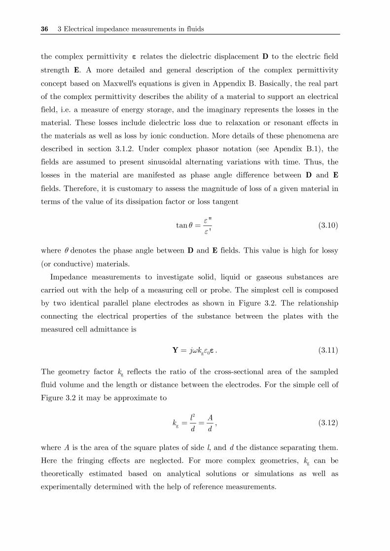
36 3 Electrical impedance measurements in fluids
the complex permittivity ε relates the dielectric displacement D to the electric field
strength E. A more detailed and general description of the complex permittivity
concept based on Maxwell's equations is given in Appendix B. Basically, the real part
of the complex permittivity describes the ability of a material to support an electrical
field, i.e. a measure of energy storage, and the imaginary represents the losses in the
material. These losses include dielectric loss due to relaxation or resonant effects in
the materials as well as loss by ionic conduction. More details of these phenomena are
described in section 3.1.2. Under complex phasor notation (see Apendix B.1), the
fields are assumed to present sinusoidal alternating variations with time. Thus, the
losses in the material are manifested as phase angle difference between D and E
fields. Therefore, it is customary to assess the magnitude of loss of a given material in
terms of the value of its dissipation factor or loss tangent
''tan'
εθε
= (3.10)
where θ denotes the phase angle between D and E fields. This value is high for lossy
(or conductive) materials.
Impedance measurements to investigate solid, liquid or gaseous substances are
carried out with the help of a measuring cell or probe. The simplest cell is composed
by two identical parallel plane electrodes as shown in Figure 3.2. The relationship
connecting the electrical properties of the substance between the plates with the
measured cell admittance is
g 0j kω ε=Y ε . (3.11)
The geometry factor kg reflects the ratio of the cross-sectional area of the sampled
fluid volume and the length or distance between the electrodes. For the simple cell of
Figure 3.2 it may be approximate to
2
gl Akd d
= = , (3.12)
where A is the area of the square plates of side l, and d the distance separating them.
Here the fringing effects are neglected. For more complex geometries, kg can be
theoretically estimated based on analytical solutions or simulations as well as
experimentally determined with the help of reference measurements.
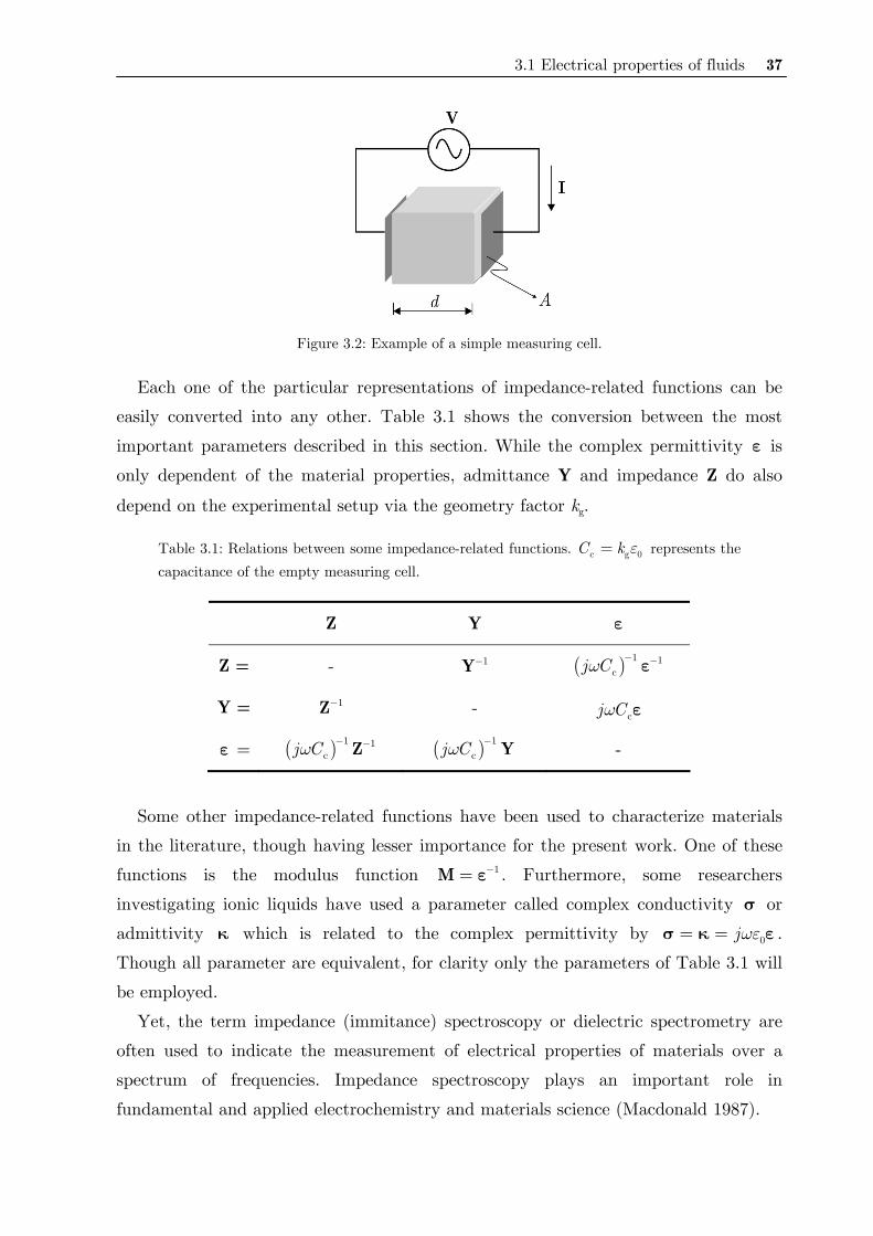
3.1 Electrical properties of fluids 37
Figure 3.2: Example of a simple measuring cell.
Each one of the particular representations of impedance-related functions can be
easily converted into any other. Table 3.1 shows the conversion between the most
important parameters described in this section. While the complex permittivity ε is
only dependent of the material properties, admittance Y and impedance Z do also
depend on the experimental setup via the geometry factor kg.
Table 3.1: Relations between some impedance-related functions. c g 0C k ε= represents the capacitance of the empty measuring cell.
Z Y ε
Z = - Y−1 ( ) 1 1cj Cω − −ε
Y = Z−1 - cj Cω ε
ε = ( ) 1 1cj Cω − −Z ( ) 1
cj Cω − Y -
Some other impedance-related functions have been used to characterize materials
in the literature, though having lesser importance for the present work. One of these
functions is the modulus function 1−=M ε . Furthermore, some researchers
investigating ionic liquids have used a parameter called complex conductivity σ or
admittivity κ which is related to the complex permittivity by 0jωε= =σ κ ε .
Though all parameter are equivalent, for clarity only the parameters of Table 3.1 will
be employed.
Yet, the term impedance (immitance) spectroscopy or dielectric spectrometry are
often used to indicate the measurement of electrical properties of materials over a
spectrum of frequencies. Impedance spectroscopy plays an important role in
fundamental and applied electrochemistry and materials science (Macdonald 1987).
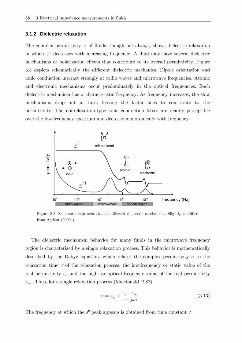
38 3 Electrical impedance measurements in fluids
3.1.2 Dielectric relaxation
The complex permittivity ε of fluids, though not always, shows dielectric relaxation
in which 'ε decreases with increasing frequency. A fluid may have several dielectric
mechanisms or polarization effects that contribute to its overall permittivity. Figure
3.3 depicts schematically the different dielectric mechanics. Dipole orientation and
ionic conduction interact strongly at radio waves and microwave frequencies. Atomic
and electronic mechanisms occur predominately in the optical frequencies. Each
dielectric mechanism has a characteristic frequency. As frequency increases, the slow
mechanisms drop out in turn, leaving the faster ones to contribute to the
permittivity. The nonrelaxation-type ionic conduction losses are readily perceptible
over the low-frequency spectrum and decrease monotonically with frequency.
Figure 3.3: Schematic representation of different dielectric mechanism. Slightly modified from Agilent (2006a).
The dielectric mechanism behavior for many fluids in the microwave frequency
region is characterized by a single relaxation process. This behavior is mathematically
described by the Debye equation, which relates the complex permittivity ε to the
relaxation time τ of the relaxation process, the low-frequency or static value of the
real permittivity εs, and the high- or optical-frequency value of the real permittivity
ε∞ . Thus, for a single relaxation process (Macdonald 1987)
s
1 jε εε
ωτ∞
∞−= +
+ε . (3.13)
The frequency at which the ε'' peak appears is obtained from time constant τ
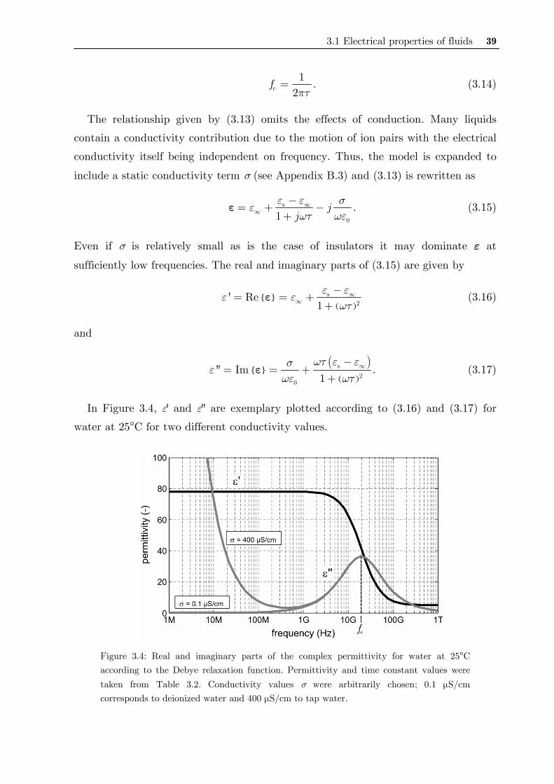
3.1 Electrical properties of fluids 39
c1
2f
πτ= . (3.14)
The relationship given by (3.13) omits the effects of conduction. Many liquids
contain a conductivity contribution due to the motion of ion pairs with the electrical
conductivity itself being independent on frequency. Thus, the model is expanded to
include a static conductivity term σ (see Appendix B.3) and (3.13) is rewritten as
s
01j
jε ε σε
ωτ ωε∞
∞−= + −
+ε . (3.15)
Even if σ is relatively small as is the case of insulators it may dominate ε at
sufficiently low frequencies. The real and imaginary parts of (3.15) are given by
( )
s2
' Re1ε εε ε
ωτ∞
∞−= = +
+ε (3.16)
and
( )
( )
s2
0
'' Im1
ωτ ε εσεωε ωτ
∞−= = +
+ε . (3.17)
In Figure 3.4, ε' and ε'' are exemplary plotted according to (3.16) and (3.17) for
water at 25°C for two different conductivity values.
Figure 3.4: Real and imaginary parts of the complex permittivity for water at 25°C according to the Debye relaxation function. Permittivity and time constant values were taken from Table 3.2. Conductivity values σ were arbitrarily chosen; 0.1 μS/cm corresponds to deionized water and 400 μS/cm to tap water.
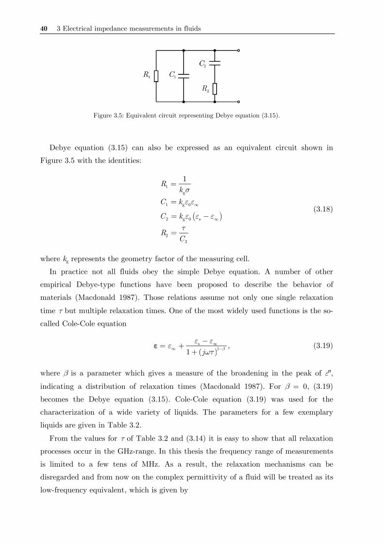
40 3 Electrical impedance measurements in fluids
Figure 3.5: Equivalent circuit representing Debye equation (3.15).
Debye equation (3.15) can also be expressed as an equivalent circuit shown in
Figure 3.5 with the identities:
( )
1g
1 g 0
2 g 0 s
22
1Rk
C k
C k
RC
σε ε
ε ε ετ
∞
∞
=
=
= −
=
(3.18)
where kg represents the geometry factor of the measuring cell.
In practice not all fluids obey the simple Debye equation. A number of other
empirical Debye-type functions have been proposed to describe the behavior of
materials (Macdonald 1987). Those relations assume not only one single relaxation
time τ but multiple relaxation times. One of the most widely used functions is the so-
called Cole-Cole equation
( )s
11 j βε εε
ωτ∞
∞ −−= +
+ε , (3.19)
where β is a parameter which gives a measure of the broadening in the peak of ε'', indicating a distribution of relaxation times (Macdonald 1987). For β = 0, (3.19)
becomes the Debye equation (3.15). Cole-Cole equation (3.19) was used for the
characterization of a wide variety of liquids. The parameters for a few exemplary
liquids are given in Table 3.2.
From the values for τ of Table 3.2 and (3.14) it is easy to show that all relaxation
processes occur in the GHz-range. In this thesis the frequency range of measurements
is limited to a few tens of MHz. As a result, the relaxation mechanisms can be
disregarded and from now on the complex permittivity of a fluid will be treated as its
low-frequency equivalent, which is given by

3.2 Impedance measuring techniques 41
0
j σεωε
= −ε , (3.20)
where ε will be used to represent the static relative permittivity εs (sometimes called
the dielectric constant). Furthermore, the equivalent low-frequency circuit of a liquid
is given by the parallel connection of a capacitor and a resistor, whose admittance is
obtained by putting (3.20) in (3.11), yielding
( )g 0k jσ ωε ε= +Y . (3.21)
Separating (3.21) in real and imaginary parts and remembering that Y = G + jωC,
the conductance G and the capacitance C are obtained as follows.
g
g 0
G k
C k
σ
ε ε
=
= (3.22)
Table 3.2: Dielectric relaxation parameters for selected liquids at 25°C. All values except that one for crude oil were taken from Buckley and Maryott (1958). Crude oil values according to Folgerø (1998).
Substance ε∞ sε β τ (ps)
2-Propanol 3.2 20 0 291.78
Air 1 - - -
Crude oil 2.32 2.19 0.52 11.30
Diethyl Ether 1.82 4.24 0 2.17
Ethanol 4.2 24 0 127.85
Ethylene Glycol 3 37 0.23 79.57
Water (deionized) 5 78 0 8.08
3.2 Impedance measuring techniques
3.2.1 Overview
Since impedance is a complex quantity, one must determine two parameters:
magnitude and phase or real and imaginary part of voltages or currents, commonly
denominated as vector measurements. The general approach to measure impedance is
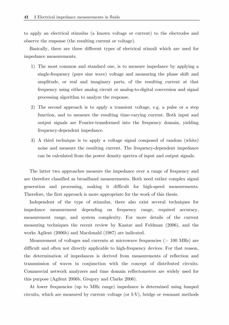
42 3 Electrical impedance measurements in fluids
to apply an electrical stimulus (a known voltage or current) to the electrodes and
observe the response (the resulting current or voltage).
Basically, there are three different types of electrical stimuli which are used for
impedance measurements.
1) The most common and standard one, is to measure impedance by applying a
single-frequency (pure sine wave) voltage and measuring the phase shift and
amplitude, or real and imaginary parts, of the resulting current at that
frequency using either analog circuit or analog-to-digital conversion and signal
processing algorithm to analyze the response.
2) The second approach is to apply a transient voltage, e.g. a pulse or a step
function, and to measure the resulting time-varying current. Both input and
output signals are Fourier-transformed into the frequency domain, yielding
frequency-dependent impedance.
3) A third technique is to apply a voltage signal composed of random (white)
noise and measure the resulting current. The frequency-dependent impedance
can be calculated from the power density spectra of input and output signals.
The latter two approaches measure the impedance over a range of frequency and
are therefore classified as broadband measurements. Both need rather complex signal
generation and processing, making it difficult for high-speed measurements.
Therefore, the first approach is more appropriate for the work of this thesis.
Independent of the type of stimulus, there also exist several techniques for
impedance measurement depending on frequency range, required accuracy,
measurement range, and system complexity. For more details of the current
measuring techniques the recent review by Kaatze and Feldman (2006), and the
works Agilent (2006b) and Macdonald (1987) are indicated.
Measurement of voltages and currents at microwave frequencies (> 100 MHz) are
difficult and often not directly applicable to high-frequency devices. For that reason,
the determination of impedances is derived from measurements of reflection and
transmission of waves in conjunction with the concept of distributed circuits.
Commercial network analyzers and time domain reflectometers are widely used for
this purpose (Agilent 2006b, Gregory and Clarke 2006).
At lower frequencies (up to MHz range) impedance is determined using lumped
circuits, which are measured by current–voltage (or I-V), bridge or resonant methods
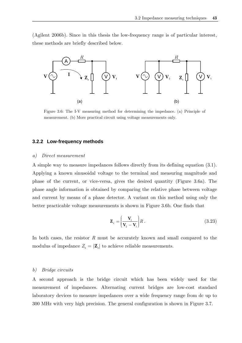
3.2 Impedance measuring techniques 43
(Agilent 2006b). Since in this thesis the low-frequency range is of particular interest,
these methods are briefly described below.
Figure 3.6: The I-V measuring method for determining the impedance. (a) Principle of measurement. (b) More practical circuit using voltage measurements only.
3.2.2 Low-frequency methods
a) Direct measurement
A simple way to measure impedances follows directly from its defining equation (3.1).
Applying a known sinusoidal voltage to the terminal and measuring magnitude and
phase of the current, or vice-versa, gives the desired quantity (Figure 3.6a). The
phase angle information is obtained by comparing the relative phase between voltage
and current by means of a phase detector. A variant on this method using only the
better practicable voltage measurements is shown in Figure 3.6b. One finds that
1x
2 1
R⎛ ⎞⎟⎜ ⎟= ⎜ ⎟⎜ ⎟⎜ −⎝ ⎠
VZV V
. (3.23)
In both cases, the resistor R must be accurately known and small compared to the
modulus of impedance Zx = |Zx| to achieve reliable measurements.
b) Bridge circuits
A second approach is the bridge circuit which has been widely used for the
measurement of impedances. Alternating current bridges are low-cost standard
laboratory devices to measure impedances over a wide frequency range from dc up to
300 MHz with very high precision. The general configuration is shown in Figure 3.7.
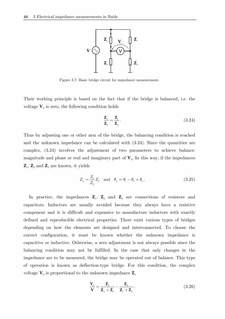
44 3 Electrical impedance measurements in fluids
Figure 3.7: Basic bridge circuit for impedance measurement.
Their working principle is based on the fact that if the bridge is balanced, i.e. the
voltage Vd is zero, the following condition holds
x 1
2 3
=Z ZZ Z
. (3.24)
Thus by adjusting one or other arm of the bridge, the balancing condition is reached
and the unknown impedance can be calculated with (3.24). Since the quantities are
complex, (3.24) involves the adjustment of two parameters to achieve balance:
magnitude and phase or real and imaginary part of Vd. In this way, if the impedances
Z1, Z2 and Z3 are known, it yields
1x 2 x 1 3 2
3
andZZ ZZ
θ θ θ θ= = − + . (3.25)
In practice, the impedances Z1, Z2 and Z3 are connections of resistors and
capacitors. Inductors are usually avoided because they always have a resistive
component and it is difficult and expensive to manufacture inductors with exactly
defined and reproducible electrical properties. There exist various types of bridges
depending on how the elements are designed and interconnected. To choose the
correct configuration, it must be known whether the unknown impedance is
capacitive or inductive. Otherwise, a zero adjustment is not always possible since the
balancing condition may not be fulfilled. In the case that only changes in the
impedance are to be measured, the bridge may be operated out of balance. This type
of operation is known as deflection-type bridge. For this condition, the complex
voltage Vd is proportional to the unknown impedance Zx
d 2 3
x 2 1 3
= −+ +
V Z ZV Z Z Z Z
. (3.26)

3.2 Impedance measuring techniques 45
Frequently used bridge circuits are the Wheatstone, Hay, Maxwell and Schering
Bridge (Oliver and Cage 1971, Morris 2001, Bera and Chattopadhyay 2003).
c) Resonant methods
The third method is called resonant method. As its name already indicates, it makes
use of the resonance effect of LC circuits to determine the impedance. Typical circuit
configurations are shown in Figure 3.8. The resonant frequency is given by
r1
2f
LCπ= . (3.27)
This method also requires a previous knowledge of if the impedance under test is
capacitive or inductive in order to compose an appropriate resonant circuit. That
means, at least one component L or C must be previously known. Basically, two
strategies have been used for determining the reactance (L or C) of a resonant circuit.
The excitation frequency may be varied searching for the resonance condition, where
the measured voltage at R achieves a maximum, or the RLC network is connected
being part of an oscillator circuit, in which the output frequency is accurately
measured. Both strategies are equivalent and the unknown reactance can be obtained
using (3.27).
The fact that at resonance condition the imaginary part of circuit impedance
vanishes can be used to determine the resistive part of impedance. Hence,
rx
r
VRI
= , (3.28)
where Vr and Ir are the voltage and current values measured at resonance.
Figure 3.8: Typical resonant circuits for the measurement of impedance. (a) General principle of measurement. (b) Variant of (a) where the oscillator output frequency f is a measure of the unknown quantity (L or C).
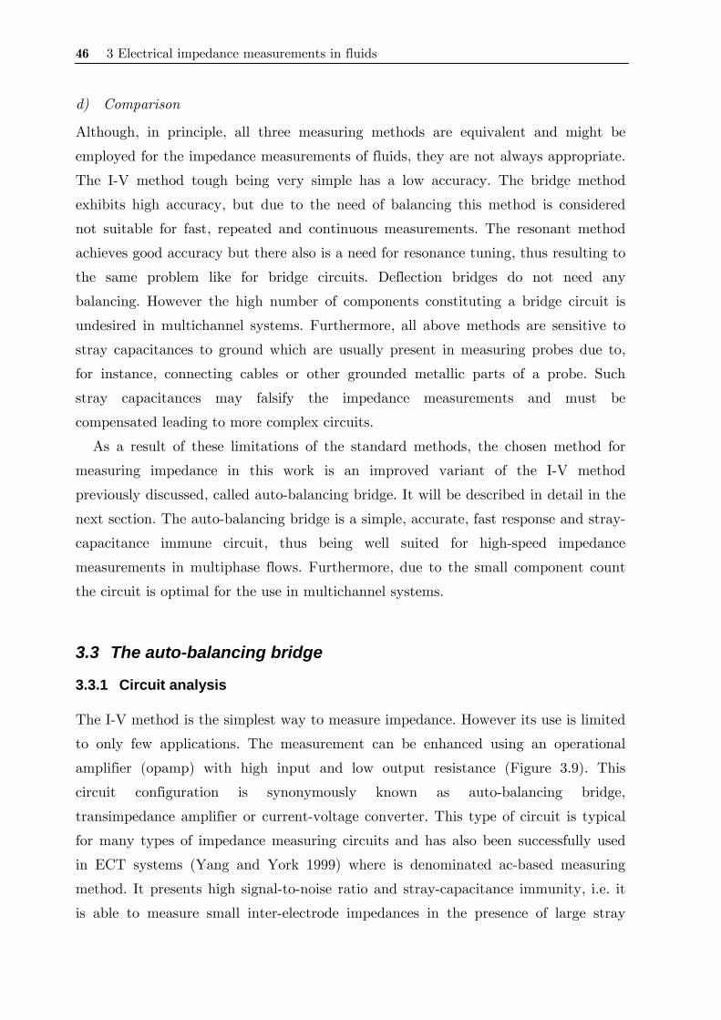
46 3 Electrical impedance measurements in fluids
d) Comparison
Although, in principle, all three measuring methods are equivalent and might be
employed for the impedance measurements of fluids, they are not always appropriate.
The I-V method tough being very simple has a low accuracy. The bridge method
exhibits high accuracy, but due to the need of balancing this method is considered
not suitable for fast, repeated and continuous measurements. The resonant method
achieves good accuracy but there also is a need for resonance tuning, thus resulting to
the same problem like for bridge circuits. Deflection bridges do not need any
balancing. However the high number of components constituting a bridge circuit is
undesired in multichannel systems. Furthermore, all above methods are sensitive to
stray capacitances to ground which are usually present in measuring probes due to,
for instance, connecting cables or other grounded metallic parts of a probe. Such
stray capacitances may falsify the impedance measurements and must be
compensated leading to more complex circuits.
As a result of these limitations of the standard methods, the chosen method for
measuring impedance in this work is an improved variant of the I-V method
previously discussed, called auto-balancing bridge. It will be described in detail in the
next section. The auto-balancing bridge is a simple, accurate, fast response and stray-
capacitance immune circuit, thus being well suited for high-speed impedance
measurements in multiphase flows. Furthermore, due to the small component count
the circuit is optimal for the use in multichannel systems.
3.3 The auto-balancing bridge
3.3.1 Circuit analysis
The I-V method is the simplest way to measure impedance. However its use is limited
to only few applications. The measurement can be enhanced using an operational
amplifier (opamp) with high input and low output resistance (Figure 3.9). This
circuit configuration is synonymously known as auto-balancing bridge,
transimpedance amplifier or current-voltage converter. This type of circuit is typical
for many types of impedance measuring circuits and has also been successfully used
in ECT systems (Yang and York 1999) where is denominated ac-based measuring
method. It presents high signal-to-noise ratio and stray-capacitance immunity, i.e. it
is able to measure small inter-electrode impedances in the presence of large stray
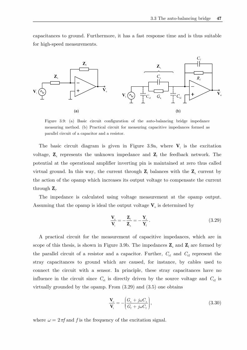
3.3 The auto-balancing bridge 47
capacitances to ground. Furthermore, it has a fast response time and is thus suitable
for high-speed measurements.
Figure 3.9: (a) Basic circuit configuration of the auto-balancing bridge impedance measuring method. (b) Practical circuit for measuring capacitive impedances formed as parallel circuit of a capacitor and a resistor.
The basic circuit diagram is given in Figure 3.9a, where Vi is the excitation
voltage, Zx represents the unknown impedance and Zf the feedback network. The
potential at the operational amplifier inverting pin is maintained at zero thus called
virtual ground. In this way, the current through Zf balances with the Zx current by
the action of the opamp which increases its output voltage to compensate the current
through Zf.
The impedance is calculated using voltage measurement at the opamp output.
Assuming that the opamp is ideal the output voltage Vo is determined by
o f x
i x f
= − = −V Z YV Z Y
. (3.29)
A practical circuit for the measurement of capacitive impedances, which are in
scope of this thesis, is shown in Figure 3.9b. The impedances Zx and Zf are formed by
the parallel circuit of a resistor and a capacitor. Further, Cs1 and Cs2 represent the
stray capacitances to ground which are caused, for instance, by cables used to
connect the circuit with a sensor. In principle, these stray capacitances have no
influence in the circuit since Cs1 is directly driven by the source voltage and Cs2 is
virtually grounded by the opamp. From (3.29) and (3.5) one obtains
o x x
i f f
G j CG j C
ωω
⎛ ⎞+ ⎟⎜ ⎟= −⎜ ⎟⎜ ⎟⎜ +⎝ ⎠VV
, (3.30)
where ω = 2πf and f is the frequency of the excitation signal.
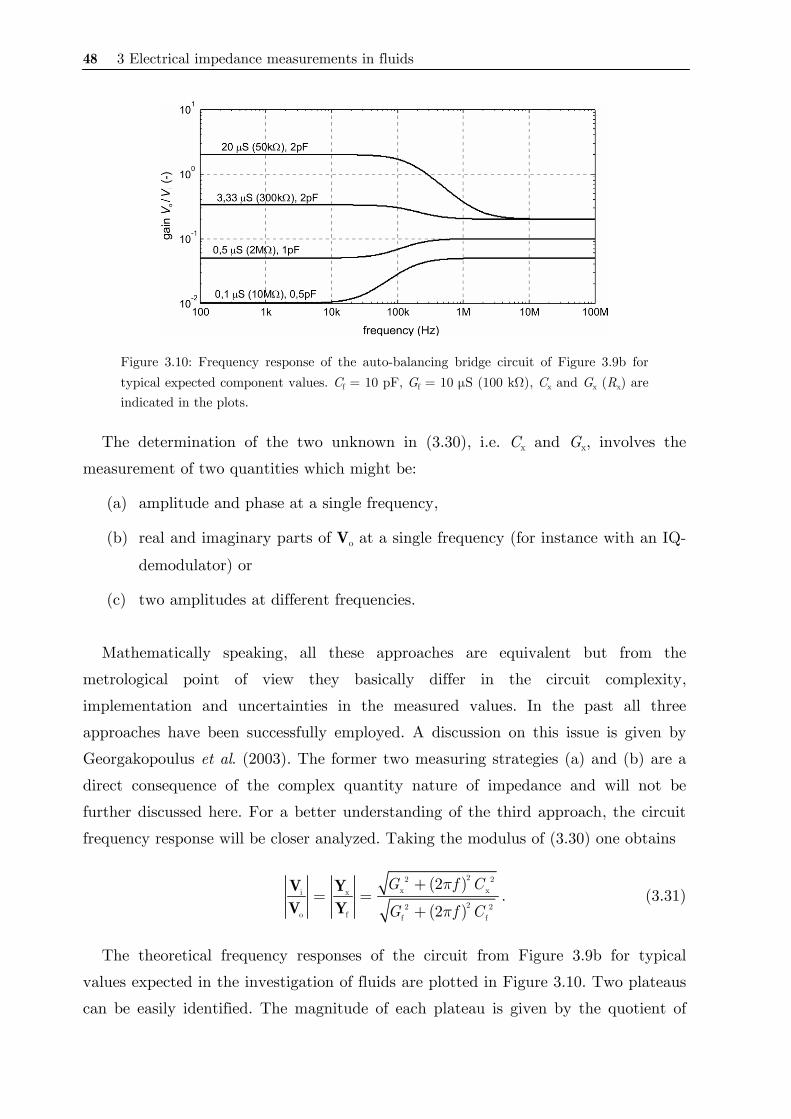
48 3 Electrical impedance measurements in fluids
Figure 3.10: Frequency response of the auto-balancing bridge circuit of Figure 3.9b for typical expected component values. Cf = 10 pF, Gf = 10 μS (100 kΩ), Cx and Gx (Rx) are indicated in the plots.
The determination of the two unknown in (3.30), i.e. Cx and Gx, involves the
measurement of two quantities which might be:
(a) amplitude and phase at a single frequency,
(b) real and imaginary parts of Vo at a single frequency (for instance with an IQ-
demodulator) or
(c) two amplitudes at different frequencies.
Mathematically speaking, all these approaches are equivalent but from the
metrological point of view they basically differ in the circuit complexity,
implementation and uncertainties in the measured values. In the past all three
approaches have been successfully employed. A discussion on this issue is given by
Georgakopoulus et al. (2003). The former two measuring strategies (a) and (b) are a
direct consequence of the complex quantity nature of impedance and will not be
further discussed here. For a better understanding of the third approach, the circuit
frequency response will be closer analyzed. Taking the modulus of (3.30) one obtains
( )( )
22 2x xi x
22 2o f f f
2
2
G f C
G f C
π
π
+= =
+V YV Y
. (3.31)
The theoretical frequency responses of the circuit from Figure 3.9b for typical
values expected in the investigation of fluids are plotted in Figure 3.10. Two plateaus
can be easily identified. The magnitude of each plateau is given by the quotient of
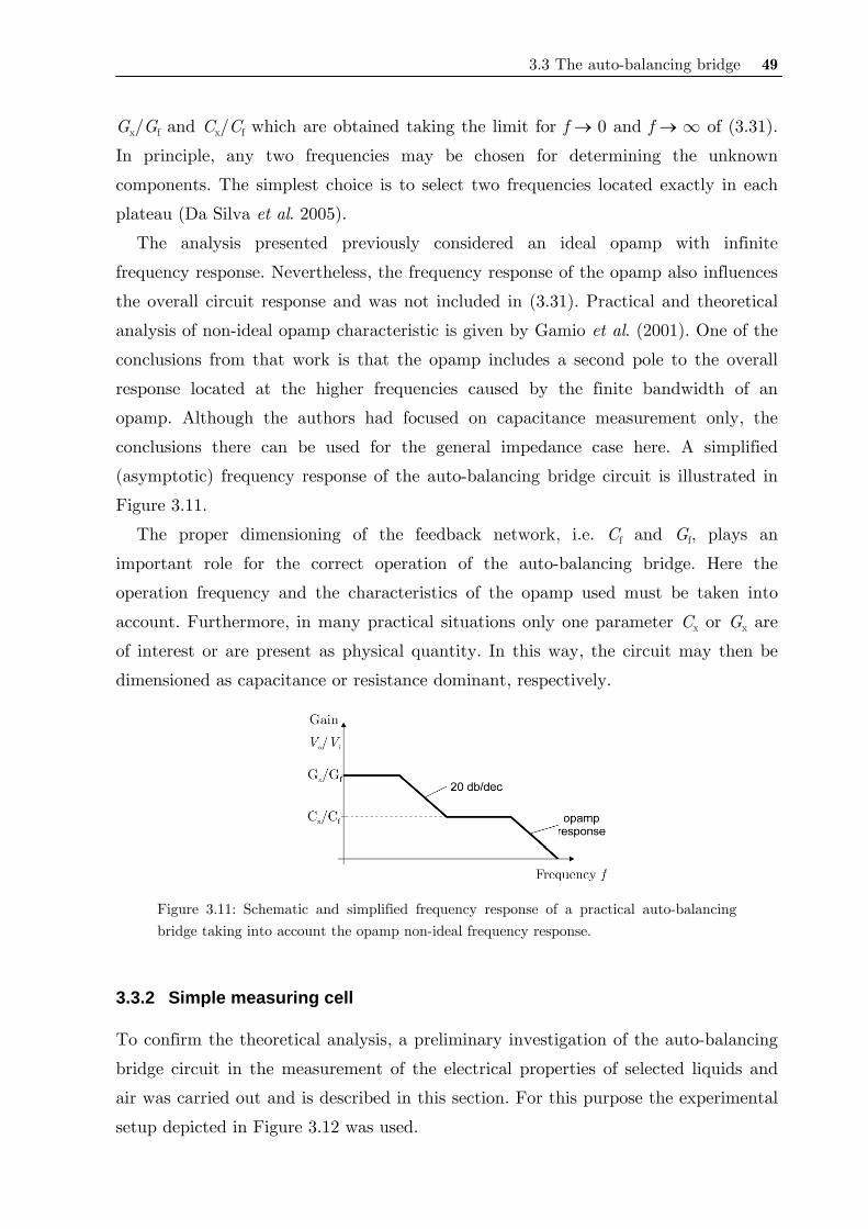
3.3 The auto-balancing bridge 49
Gx/Gf and Cx/Cf which are obtained taking the limit for f → 0 and f → ∞ of (3.31).
In principle, any two frequencies may be chosen for determining the unknown
components. The simplest choice is to select two frequencies located exactly in each
plateau (Da Silva et al. 2005).
The analysis presented previously considered an ideal opamp with infinite
frequency response. Nevertheless, the frequency response of the opamp also influences
the overall circuit response and was not included in (3.31). Practical and theoretical
analysis of non-ideal opamp characteristic is given by Gamio et al. (2001). One of the
conclusions from that work is that the opamp includes a second pole to the overall
response located at the higher frequencies caused by the finite bandwidth of an
opamp. Although the authors had focused on capacitance measurement only, the
conclusions there can be used for the general impedance case here. A simplified
(asymptotic) frequency response of the auto-balancing bridge circuit is illustrated in
Figure 3.11.
The proper dimensioning of the feedback network, i.e. Cf and Gf, plays an
important role for the correct operation of the auto-balancing bridge. Here the
operation frequency and the characteristics of the opamp used must be taken into
account. Furthermore, in many practical situations only one parameter Cx or Gx are
of interest or are present as physical quantity. In this way, the circuit may then be
dimensioned as capacitance or resistance dominant, respectively.
Figure 3.11: Schematic and simplified frequency response of a practical auto-balancing bridge taking into account the opamp non-ideal frequency response.
3.3.2 Simple measuring cell
To confirm the theoretical analysis, a preliminary investigation of the auto-balancing
bridge circuit in the measurement of the electrical properties of selected liquids and
air was carried out and is described in this section. For this purpose the experimental
setup depicted in Figure 3.12 was used.
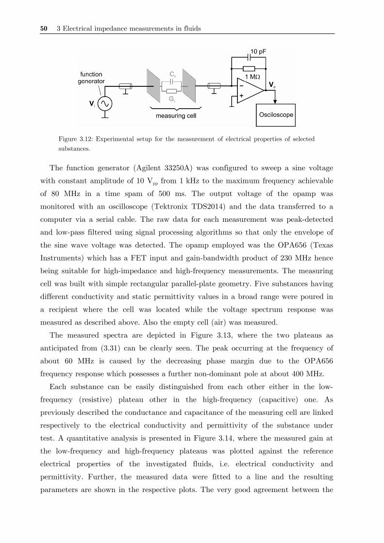
50 3 Electrical impedance measurements in fluids
Figure 3.12: Experimental setup for the measurement of electrical properties of selected substances.
The function generator (Agilent 33250A) was configured to sweep a sine voltage
with constant amplitude of 10 Vpp from 1 kHz to the maximum frequency achievable
of 80 MHz in a time spam of 500 ms. The output voltage of the opamp was
monitored with an oscilloscope (Tektronix TDS2014) and the data transferred to a
computer via a serial cable. The raw data for each measurement was peak-detected
and low-pass filtered using signal processing algorithms so that only the envelope of
the sine wave voltage was detected. The opamp employed was the OPA656 (Texas
Instruments) which has a FET input and gain-bandwidth product of 230 MHz hence
being suitable for high-impedance and high-frequency measurements. The measuring
cell was built with simple rectangular parallel-plate geometry. Five substances having
different conductivity and static permittivity values in a broad range were poured in
a recipient where the cell was located while the voltage spectrum response was
measured as described above. Also the empty cell (air) was measured.
The measured spectra are depicted in Figure 3.13, where the two plateaus as
anticipated from (3.31) can be clearly seen. The peak occurring at the frequency of
about 60 MHz is caused by the decreasing phase margin due to the OPA656
frequency response which possesses a further non-dominant pole at about 400 MHz.
Each substance can be easily distinguished from each other either in the low-
frequency (resistive) plateau other in the high-frequency (capacitive) one. As
previously described the conductance and capacitance of the measuring cell are linked
respectively to the electrical conductivity and permittivity of the substance under
test. A quantitative analysis is presented in Figure 3.14, where the measured gain at
the low-frequency and high-frequency plateaus was plotted against the reference
electrical properties of the investigated fluids, i.e. electrical conductivity and
permittivity. Further, the measured data were fitted to a line and the resulting
parameters are shown in the respective plots. The very good agreement between the
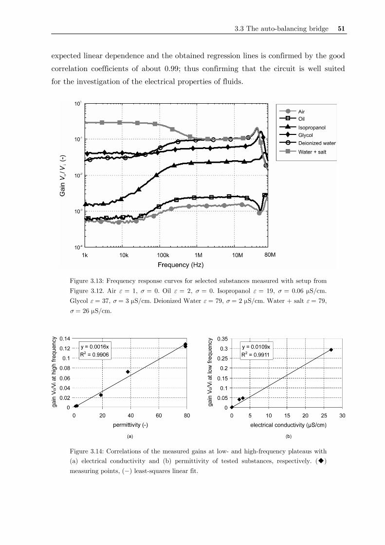
3.3 The auto-balancing bridge 51
expected linear dependence and the obtained regression lines is confirmed by the good
correlation coefficients of about 0.99; thus confirming that the circuit is well suited
for the investigation of the electrical properties of fluids.
Figure 3.13: Frequency response curves for selected substances measured with setup from Figure 3.12. Air ε = 1, σ = 0. Oil ε = 2, σ = 0. Isopropanol ε = 19, σ = 0.06 μS/cm. Glycol ε = 37, σ = 3 μS/cm. Deionized Water ε = 79, σ = 2 μS/cm. Water + salt ε = 79, σ = 26 μS/cm.
Figure 3.14: Correlations of the measured gains at low- and high-frequency plateaus with (a) electrical conductivity and (b) permittivity of tested substances, respectively. ( ) measuring points, (−) least-squares linear fit.
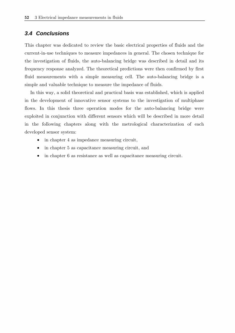
52 3 Electrical impedance measurements in fluids
3.4 Conclusions
This chapter was dedicated to review the basic electrical properties of fluids and the
current-in-use techniques to measure impedances in general. The chosen technique for
the investigation of fluids, the auto-balancing bridge was described in detail and its
frequency response analyzed. The theoretical predictions were then confirmed by first
fluid measurements with a simple measuring cell. The auto-balancing bridge is a
simple and valuable technique to measure the impedance of fluids.
In this way, a solid theoretical and practical basis was established, which is applied
in the development of innovative sensor systems to the investigation of multiphase
flows. In this thesis three operation modes for the auto-balancing bridge were
exploited in conjunction with different sensors which will be described in more detail
in the following chapters along with the metrological characterization of each
developed sensor system:
• in chapter 4 as impedance measuring circuit,
• in chapter 5 as capacitance measuring circuit, and
• in chapter 6 as resistance as well as capacitance measuring circuit.
53
4 Complex permittivity needle probe
This chapter presents a novel needle probe measuring system based
on high-speed complex permittivity measurements. The measuring
circuit is a direct application of the auto-balancing bridge circuit
discussed in the previous chapter in conjunction with a specially
designed needle probe. Such probes are able to distinguish the
different phases or components of a flow by measuring the complex
value of the electrical impedance at a high data rate.
4.1 Introduction
Measurement with local needle probes is a well-established method for the
investigation of two-phase flows (section 2.2.1a). Needle probes can identify the
phase, which is momentarily present at the location of the needle tip. Based on this
local phase information, different flow parameters can be derived. A number of
measuring principles have been employed for the needle probes in the past. Most
sensors employ conductivity, capacitance, optical and temperature measurement
techniques (Cartellier and Achard 1990). However, each one of these techniques has
limitations regarding the range of substances it is able to measure. Conductivity or
resistivity probes can only differentiate an electrically conducting phase from a non-
conducting one. Capacitances probes encounter problems when permittivities of the
two phases are similar. The same difficulty occurs with optical probes and low
refractive index differences. Temperature probes require sufficient temperature
differences in the substances, which are to be discriminated. Therefore, these probes
have been utilized almost exclusively in two-phase flow measurements.
In recent years some efforts have been made by applying dual modality measuring
techniques for enhancing the range of substances in the investigation of multiphase
flows, in which two different sensing techniques are used to distinguish the different
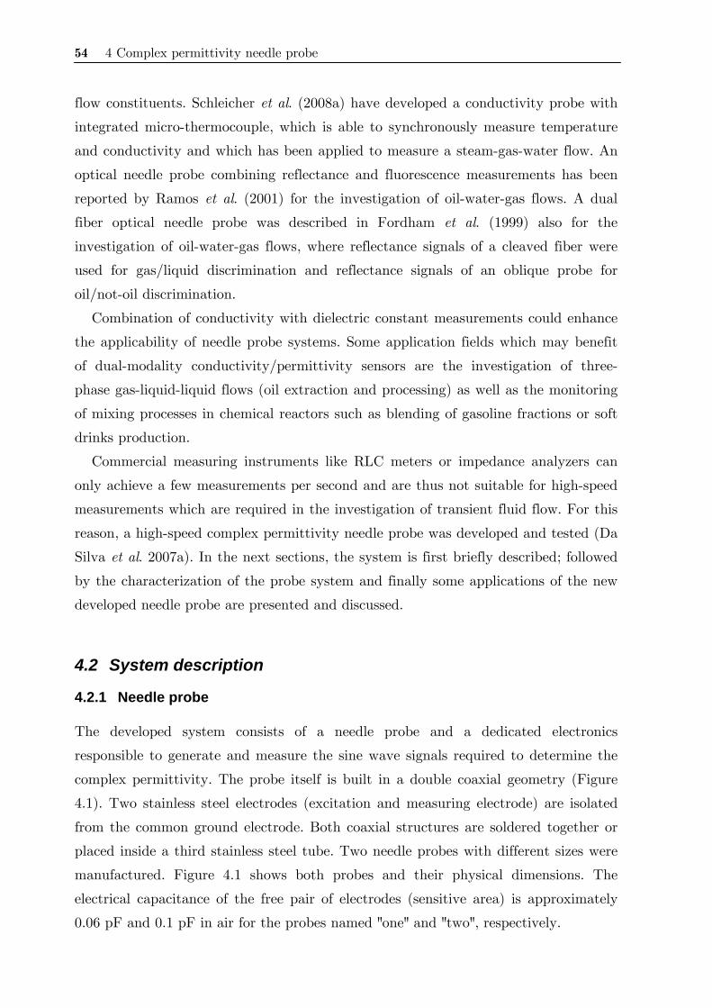
54 4 Complex permittivity needle probe
flow constituents. Schleicher et al. (2008a) have developed a conductivity probe with
integrated micro-thermocouple, which is able to synchronously measure temperature
and conductivity and which has been applied to measure a steam-gas-water flow. An
optical needle probe combining reflectance and fluorescence measurements has been
reported by Ramos et al. (2001) for the investigation of oil-water-gas flows. A dual
fiber optical needle probe was described in Fordham et al. (1999) also for the
investigation of oil-water-gas flows, where reflectance signals of a cleaved fiber were
used for gas/liquid discrimination and reflectance signals of an oblique probe for
oil/not-oil discrimination.
Combination of conductivity with dielectric constant measurements could enhance
the applicability of needle probe systems. Some application fields which may benefit
of dual-modality conductivity/permittivity sensors are the investigation of three-
phase gas-liquid-liquid flows (oil extraction and processing) as well as the monitoring
of mixing processes in chemical reactors such as blending of gasoline fractions or soft
drinks production.
Commercial measuring instruments like RLC meters or impedance analyzers can
only achieve a few measurements per second and are thus not suitable for high-speed
measurements which are required in the investigation of transient fluid flow. For this
reason, a high-speed complex permittivity needle probe was developed and tested (Da
Silva et al. 2007a). In the next sections, the system is first briefly described; followed
by the characterization of the probe system and finally some applications of the new
developed needle probe are presented and discussed.
4.2 System description
4.2.1 Needle probe
The developed system consists of a needle probe and a dedicated electronics
responsible to generate and measure the sine wave signals required to determine the
complex permittivity. The probe itself is built in a double coaxial geometry (Figure
4.1). Two stainless steel electrodes (excitation and measuring electrode) are isolated
from the common ground electrode. Both coaxial structures are soldered together or
placed inside a third stainless steel tube. Two needle probes with different sizes were
manufactured. Figure 4.1 shows both probes and their physical dimensions. The
electrical capacitance of the free pair of electrodes (sensitive area) is approximately
0.06 pF and 0.1 pF in air for the probes named "one" and "two", respectively.
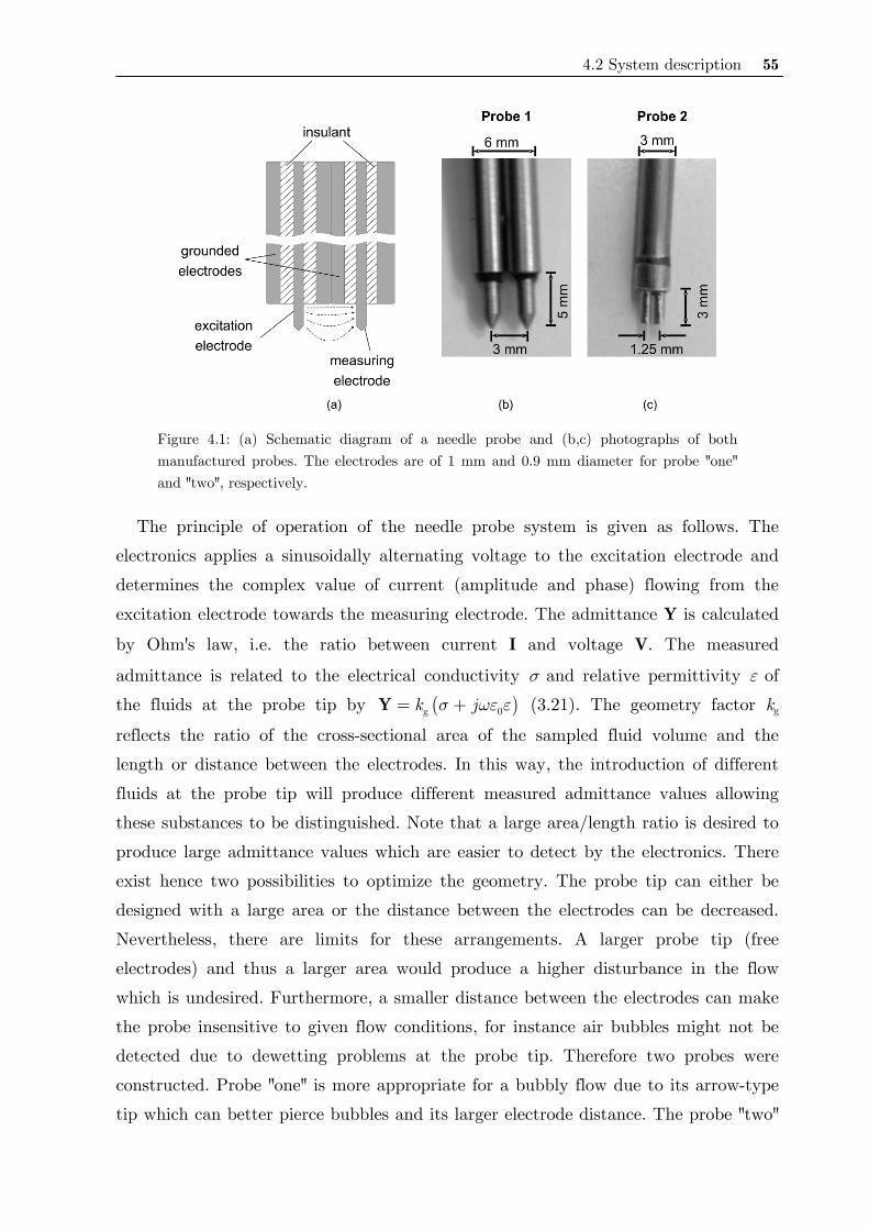
4.2 System description 55
Figure 4.1: (a) Schematic diagram of a needle probe and (b,c) photographs of both manufactured probes. The electrodes are of 1 mm and 0.9 mm diameter for probe "one" and "two", respectively.
The principle of operation of the needle probe system is given as follows. The
electronics applies a sinusoidally alternating voltage to the excitation electrode and
determines the complex value of current (amplitude and phase) flowing from the
excitation electrode towards the measuring electrode. The admittance Y is calculated
by Ohm's law, i.e. the ratio between current I and voltage V. The measured
admittance is related to the electrical conductivity σ and relative permittivity ε of
the fluids at the probe tip by ( )g 0k jσ ωε ε= +Y (3.21). The geometry factor kg
reflects the ratio of the cross-sectional area of the sampled fluid volume and the
length or distance between the electrodes. In this way, the introduction of different
fluids at the probe tip will produce different measured admittance values allowing
these substances to be distinguished. Note that a large area/length ratio is desired to
produce large admittance values which are easier to detect by the electronics. There
exist hence two possibilities to optimize the geometry. The probe tip can either be
designed with a large area or the distance between the electrodes can be decreased.
Nevertheless, there are limits for these arrangements. A larger probe tip (free
electrodes) and thus a larger area would produce a higher disturbance in the flow
which is undesired. Furthermore, a smaller distance between the electrodes can make
the probe insensitive to given flow conditions, for instance air bubbles might not be
detected due to dewetting problems at the probe tip. Therefore two probes were
constructed. Probe "one" is more appropriate for a bubbly flow due to its arrow-type
tip which can better pierce bubbles and its larger electrode distance. The probe "two"

56 4 Complex permittivity needle probe
was optimized for the investigation of a mixing process in a stirred tank which is
better described in section 4.4.2. Evidently, other scaled up or down variations of the
probe can be designed in order to adapt to other applications or constraints.
Figure 4.2: Block diagram of the electronic circuitry to measure the complex permittivity of a needle probe system.
4.2.2 Measuring electronics
A block diagram of the electronic circuitry can be seen in Figure 4.2. A direct digital
synthesizer (DDS) generates the excitation sine wave voltage. Frequencies from
100 kHz up to 1 MHz can be generated and are user-selectable. The alternating
excitation voltage Vi is supplied to the excitation electrode by means of a coaxial
cable. The measuring electrode is connected to a transimpedance amplifier also by
means of a coaxial cable. From section 3.3.1 it is known that the output voltage of
the auto-balancing bridge is a measure of the admittance under test, here
denominated Ym, hence
o i mf
1= ⋅ ⋅V V YY
, (4.1)

4.2 System description 57
where Yf is the feedback admittance. The output voltage Vo is then input to the
amplitude and phase detector block. The integrated circuit (IC) AD8302 realizes the
function of measuring amplitude and phase. This IC determines the amplitude ratio
and the phase difference from Vo and a reference signal VR. The AD8302 measures
phase differences in two quadrants (e.g. from 0° to 180°) and achieves the best
accuracy in the phase measurement only between phase differences of 20° and 160°
(nominal accuracy 0.5°). Since the phase difference caused by the needle probe was
expected to be as small as a few degrees for non-conducting substances, a phase
shifter was required to allow the AD8302 to work with highest accuracy. The phase
shifter was easily implemented by means of a second DDS, which generates a
reference voltage VR with known amplitude and digitally programmable phase.
Usually, a 90° phase delay was generated, thus placing the operation point of the
AD8302 in the center of its measuring range. For this reason, both DDS generators
are phase-synchronized by sharing the same clock source. A big advantage of a DDS-
based phase shifter is the fact that the phase shift is independent of frequency. The
two dc output signals of the AD8302, which carry the information on amplitude and
phase difference, are fed into the analog-to-digital converter (ADC), 12 bit,
20 000 samples/s per channel, of the data acquisition (DAQ) module PMD-1208FS
(Measurement and Computing Inc.). The DAQ module is connected to a PC through
a USB port. The digital port of the DAQ module is used to program the DDS sine
generators. Furthermore, a control and measurement software in the PC determines
the frequency and phase lag of each DDS, controls the analog-to-digital conversion
sequence and realizes the calculation of the admittance from the measured amplitude
and phase values. A detailed description of the design and implementation of the
system can be found in the diploma thesis Brückner (2005).
4.2.3 Complex permittivity measurement
The measuring admittance Ym represents the sum of the fluid admittance Yx and a
residual admittance YR (e.g. stray capacitance, resistance and inductance of cables,
etc.) though being small, this residual admittance falsifies the measurement and a
calibration routine is thus necessary. Equation (4.1) is modified to
x Ro i
f
+= −Y YV VY
. (4.2)
58 4 Complex permittivity needle probe
From (4.2), it can be shown that the fluid admittance Yx is linearly dependent on the
measured output voltage Vo in the form
x o= + ⋅Y A B V , (4.3)
where A and B are proportionality factors. As mentioned in section 3.1.1, fluids are
better characterized by their complex permittivity rather than their impedance or
admittance. According to theory described there, the admittance of the probe and the
complex permittivity of the fluid at probe's tip are directly proportional. In this way,
from (4.3) and (3.11) one obtains
x o= + ⋅C D Vε . (4.4)
Therefore, a two-point calibration is sufficient to determine the system variables C
and D. For that, two known reference substances with known complex permittivity
(ε1 and ε2) may be connected to the probe and Vo measured for both conditions
obtaining Vo1 and Vo2. The values for system variables are then determined from
2 o1 1 o1
o1 o2
⋅ − ⋅=−
V VCV V
ε ε , (4.5)
2 1
o1 o2
−=−
DV Vε ε . (4.6)
With the help of the above formulae, it is now possible to calibrate a complex
permittivity needle probe at two materials with known electrical properties, e.g. air
and water. In the case, one is interested only to differentiate the phases or
components of a fluid flow, e.g. gas phase detection in a bubbly flow, the calibration
procedure is not anymore necessary, since the measured voltage Vo already carries
this information in its complex value. Each component or phase is associated to a
point in the complex plane. Thus, this value can be evaluated directly to determine
the phase/component indicator function (2.1) and derived parameters.
4.3 Measurement uncertainty
System outputs, i.e. amplitude and phase measurements, were evaluated for drift and
random noise. A 100 kΩ resistor was connected to the needle probe electrodes and the
outputs were monitored for one hour at maximum sampling rate of 20 kS/s. A one-

4.3 Measurement uncertainty 59
minute moving-average filter was used to reduce random noise for determination of
the drift. System drift was defined as maximum deviation of the outputs over the
period. The measured drift was 34.13 mV and 0.637°. Random noise was estimated as
the standard deviation of the signals over a time equal to one minute. Measured
random noise was 14.42 mV and 0.272°. Applying the uncertainty propagation rules
(ISO 1995) in (4.4), one can estimate both the drift and random noise for the
complex permittivity parameter:
( ) ( )oU U= ⋅D Vε , (4.7)
where U(ε) represents the uncertainty in the complex permittivity, U(Vo) the
uncertainty in the measured output voltage and D is defined in (4.4). Drift and
random noise were then calculated from (4.7) by using typical calibration values for
D. Drift values were 0.4272 and 0.0023 μS/cm for permittivity and conductivity,
respectively. Furthermore, random noise value was 0.1810 for permittivity and
0.0009 μS/cm for conductivity.
The system was also tested in measuring different liquids and air. The liquids were
put in a metal cylinder of 10 cm in height, 10 cm in diameter and the probe was
located in the center. First, the system was calibrated by measuring air (empty
probe) and deionized water. The excitation frequency was 200 kHz and sampling
frequency 20 kS/s. The measurements were carried out with both needle probe
designs.
Figure 4.3: Results of conductivity (a) and permittivity (b) measurement by the needle probe compared with reference values. The dashed lines represent a deviation of 7% from the ideal line (−).
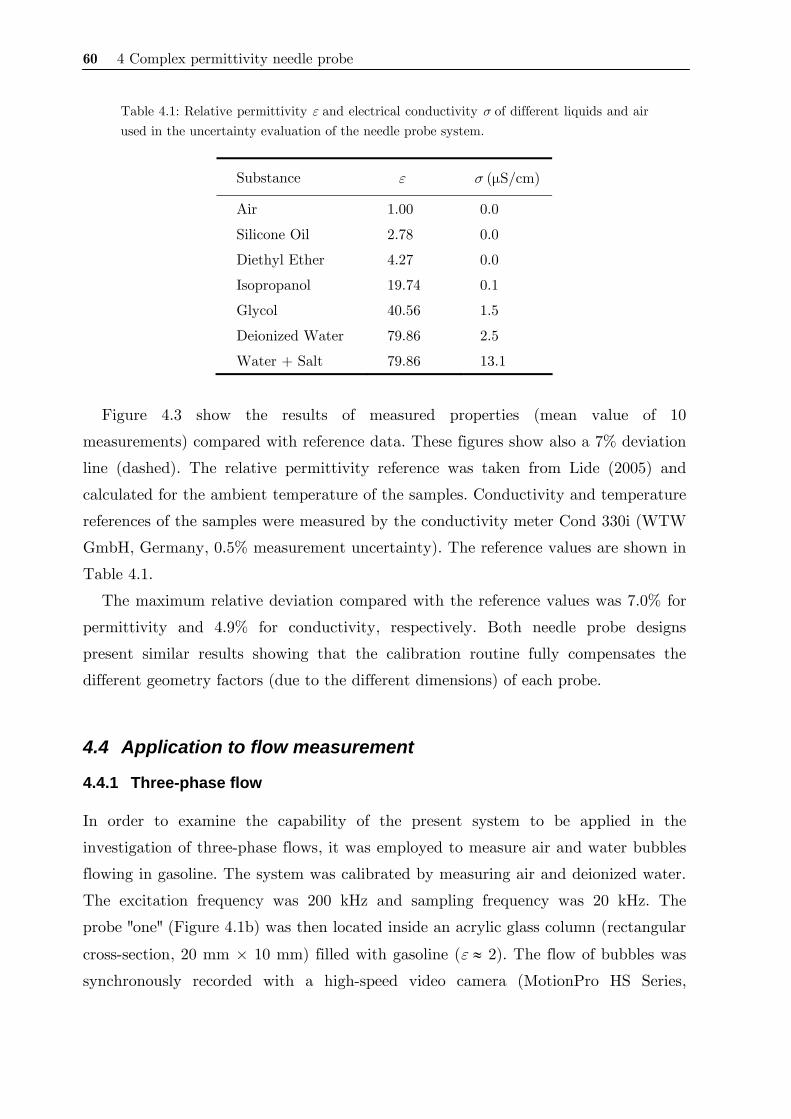
60 4 Complex permittivity needle probe
Table 4.1: Relative permittivity ε and electrical conductivity σ of different liquids and air used in the uncertainty evaluation of the needle probe system.
Substance ε σ (μS/cm)
Air 1.00 0.0
Silicone Oil 2.78 0.0
Diethyl Ether 4.27 0.0
Isopropanol 19.74 0.1
Glycol 40.56 1.5
Deionized Water 79.86 2.5
Water + Salt 79.86 13.1
Figure 4.3 show the results of measured properties (mean value of 10
measurements) compared with reference data. These figures show also a 7% deviation
line (dashed). The relative permittivity reference was taken from Lide (2005) and
calculated for the ambient temperature of the samples. Conductivity and temperature
references of the samples were measured by the conductivity meter Cond 330i (WTW
GmbH, Germany, 0.5% measurement uncertainty). The reference values are shown in
Table 4.1.
The maximum relative deviation compared with the reference values was 7.0% for
permittivity and 4.9% for conductivity, respectively. Both needle probe designs
present similar results showing that the calibration routine fully compensates the
different geometry factors (due to the different dimensions) of each probe.
4.4 Application to flow measurement
4.4.1 Three-phase flow
In order to examine the capability of the present system to be applied in the
investigation of three-phase flows, it was employed to measure air and water bubbles
flowing in gasoline. The system was calibrated by measuring air and deionized water.
The excitation frequency was 200 kHz and sampling frequency was 20 kHz. The
probe "one" (Figure 4.1b) was then located inside an acrylic glass column (rectangular
cross-section, 20 mm × 10 mm) filled with gasoline (ε ≈ 2). The flow of bubbles was
synchronously recorded with a high-speed video camera (MotionPro HS Series,
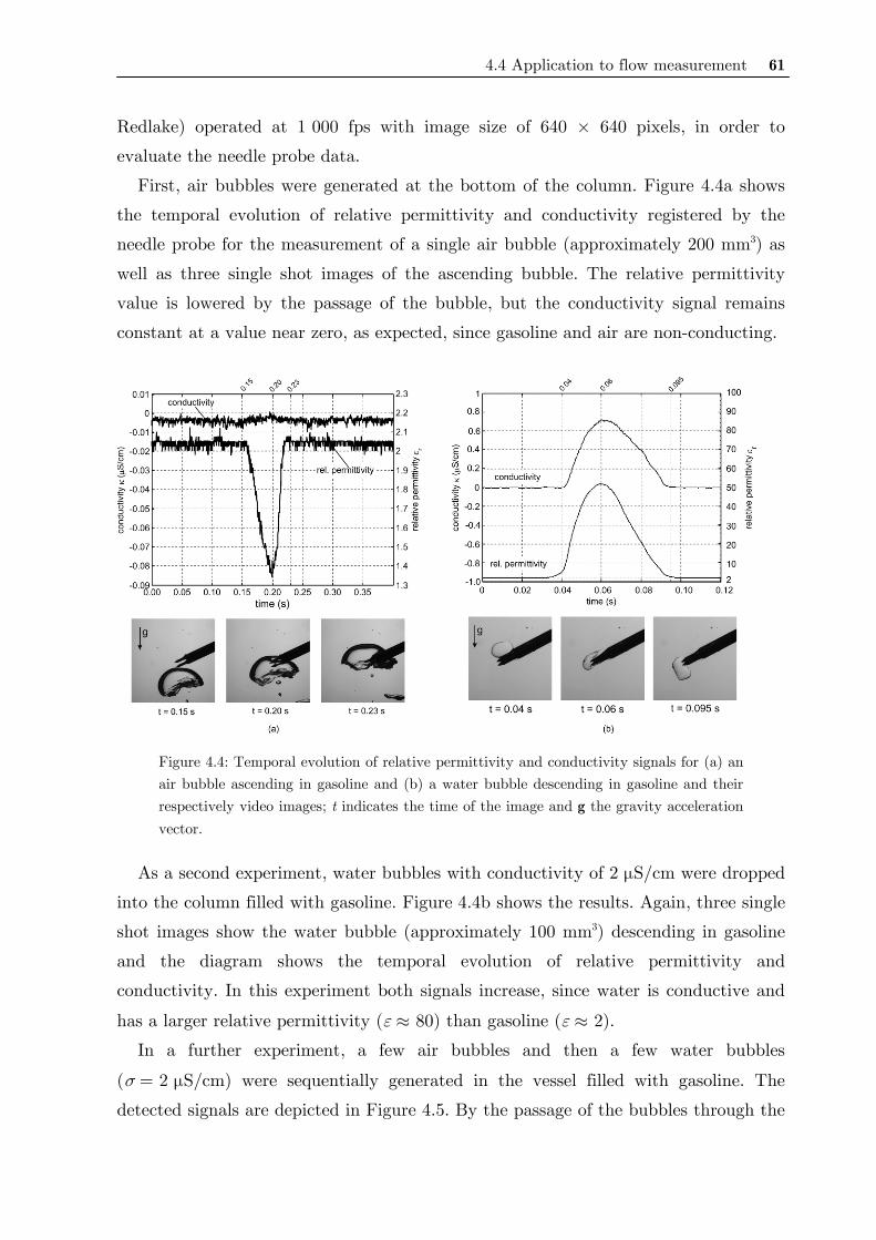
4.4 Application to flow measurement 61
Redlake) operated at 1 000 fps with image size of 640 × 640 pixels, in order to
evaluate the needle probe data.
First, air bubbles were generated at the bottom of the column. Figure 4.4a shows
the temporal evolution of relative permittivity and conductivity registered by the
needle probe for the measurement of a single air bubble (approximately 200 mm3) as
well as three single shot images of the ascending bubble. The relative permittivity
value is lowered by the passage of the bubble, but the conductivity signal remains
constant at a value near zero, as expected, since gasoline and air are non-conducting.
Figure 4.4: Temporal evolution of relative permittivity and conductivity signals for (a) an air bubble ascending in gasoline and (b) a water bubble descending in gasoline and their respectively video images; t indicates the time of the image and g the gravity acceleration vector.
As a second experiment, water bubbles with conductivity of 2 μS/cm were dropped
into the column filled with gasoline. Figure 4.4b shows the results. Again, three single
shot images show the water bubble (approximately 100 mm3) descending in gasoline
and the diagram shows the temporal evolution of relative permittivity and
conductivity. In this experiment both signals increase, since water is conductive and
has a larger relative permittivity (ε ≈ 80) than gasoline (ε ≈ 2).
In a further experiment, a few air bubbles and then a few water bubbles
(σ = 2 μS/cm) were sequentially generated in the vessel filled with gasoline. The
detected signals are depicted in Figure 4.5. By the passage of the bubbles through the
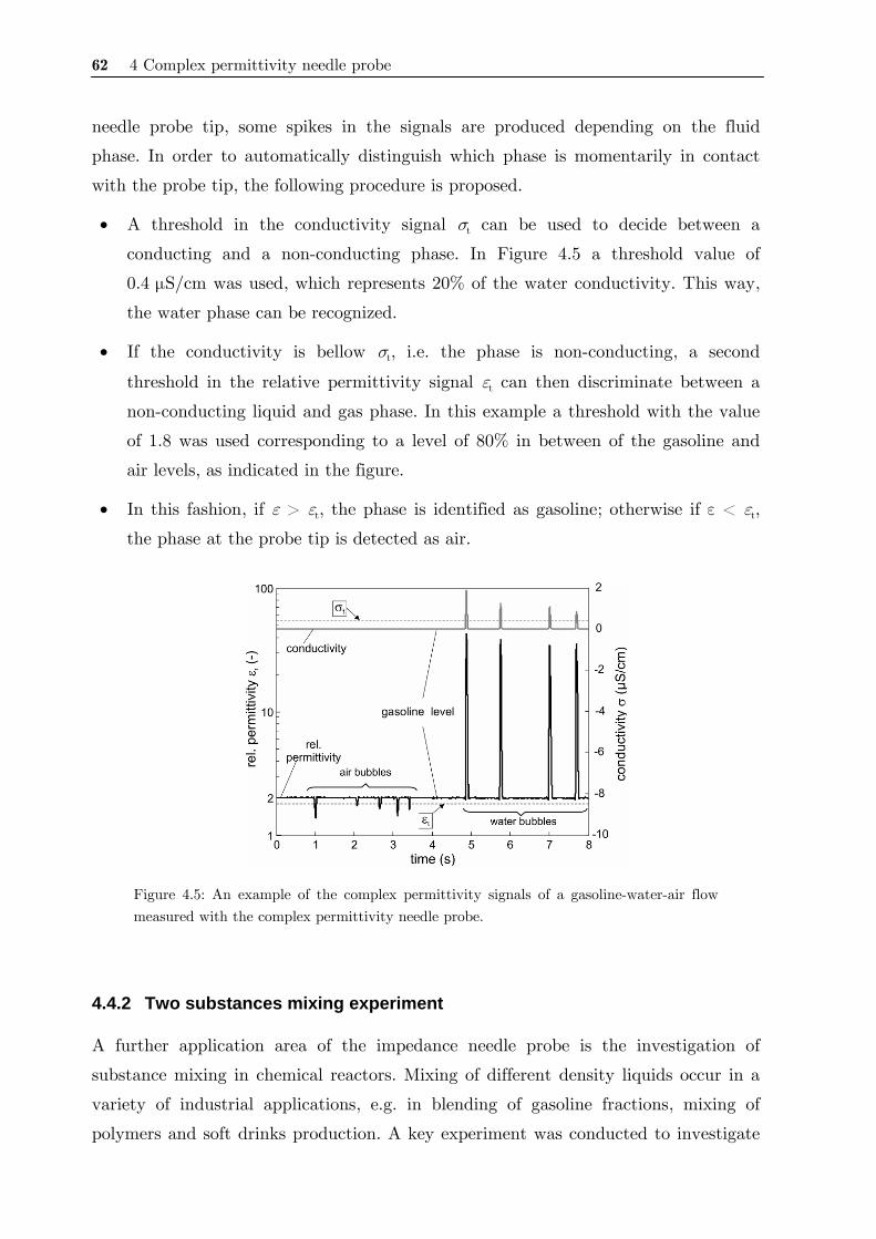
62 4 Complex permittivity needle probe
needle probe tip, some spikes in the signals are produced depending on the fluid
phase. In order to automatically distinguish which phase is momentarily in contact
with the probe tip, the following procedure is proposed.
• A threshold in the conductivity signal σt can be used to decide between a
conducting and a non-conducting phase. In Figure 4.5 a threshold value of
0.4 μS/cm was used, which represents 20% of the water conductivity. This way,
the water phase can be recognized.
• If the conductivity is bellow σt, i.e. the phase is non-conducting, a second
threshold in the relative permittivity signal εt can then discriminate between a
non-conducting liquid and gas phase. In this example a threshold with the value
of 1.8 was used corresponding to a level of 80% in between of the gasoline and
air levels, as indicated in the figure.
• In this fashion, if ε > εt, the phase is identified as gasoline; otherwise if ε < εt,
the phase at the probe tip is detected as air.
Figure 4.5: An example of the complex permittivity signals of a gasoline-water-air flow measured with the complex permittivity needle probe.
4.4.2 Two substances mixing experiment
A further application area of the impedance needle probe is the investigation of
substance mixing in chemical reactors. Mixing of different density liquids occur in a
variety of industrial applications, e.g. in blending of gasoline fractions, mixing of
polymers and soft drinks production. A key experiment was conducted to investigate
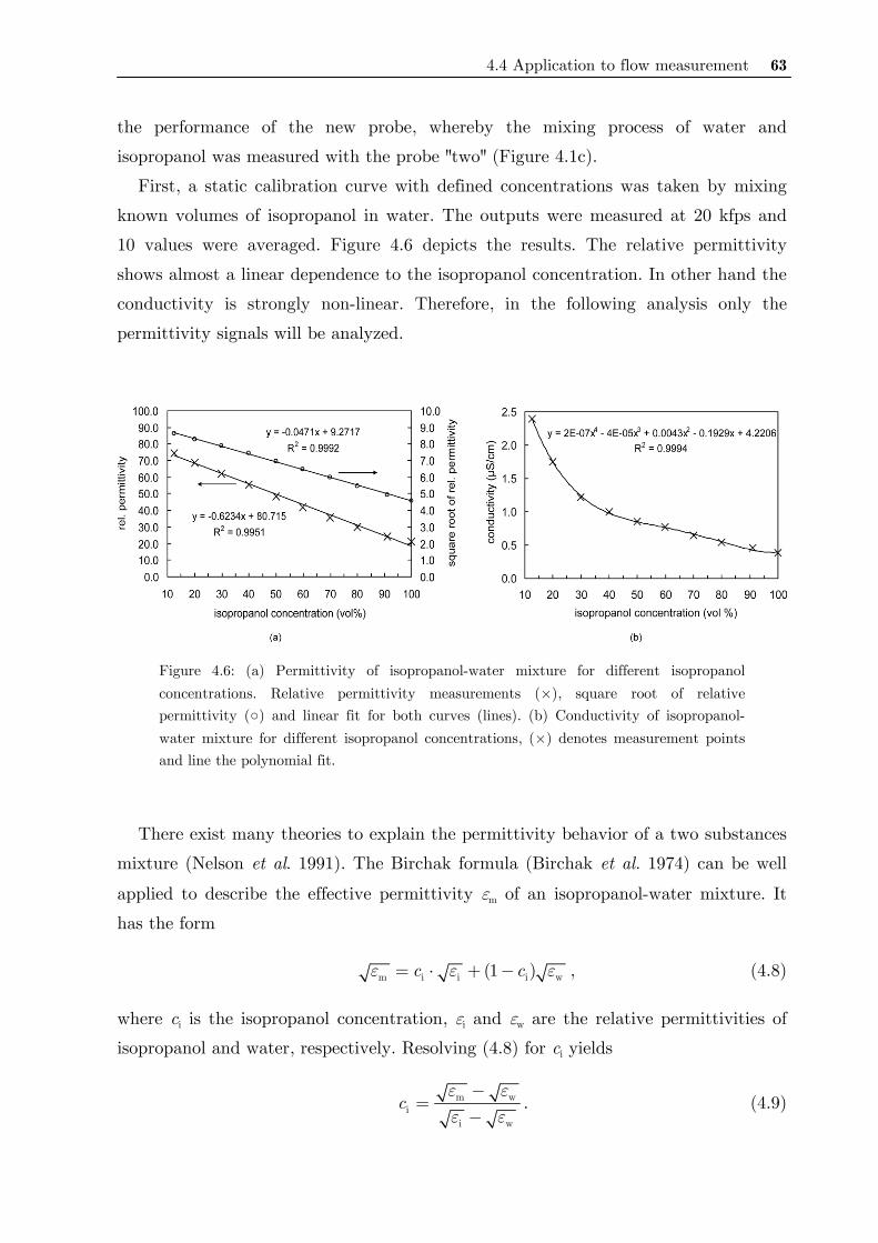
4.4 Application to flow measurement 63
the performance of the new probe, whereby the mixing process of water and
isopropanol was measured with the probe "two" (Figure 4.1c).
First, a static calibration curve with defined concentrations was taken by mixing
known volumes of isopropanol in water. The outputs were measured at 20 kfps and
10 values were averaged. Figure 4.6 depicts the results. The relative permittivity
shows almost a linear dependence to the isopropanol concentration. In other hand the
conductivity is strongly non-linear. Therefore, in the following analysis only the
permittivity signals will be analyzed.
Figure 4.6: (a) Permittivity of isopropanol-water mixture for different isopropanol concentrations. Relative permittivity measurements (×), square root of relative permittivity () and linear fit for both curves (lines). (b) Conductivity of isopropanol-water mixture for different isopropanol concentrations, (×) denotes measurement points and line the polynomial fit.
There exist many theories to explain the permittivity behavior of a two substances
mixture (Nelson et al. 1991). The Birchak formula (Birchak et al. 1974) can be well
applied to describe the effective permittivity εm of an isopropanol-water mixture. It
has the form
m i i i w(1 )c cε ε ε= ⋅ + − , (4.8)
where ci is the isopropanol concentration, εi and εw are the relative permittivities of
isopropanol and water, respectively. Resolving (4.8) for ci yields
m wi
i w
cε εε ε
−=
−. (4.9)
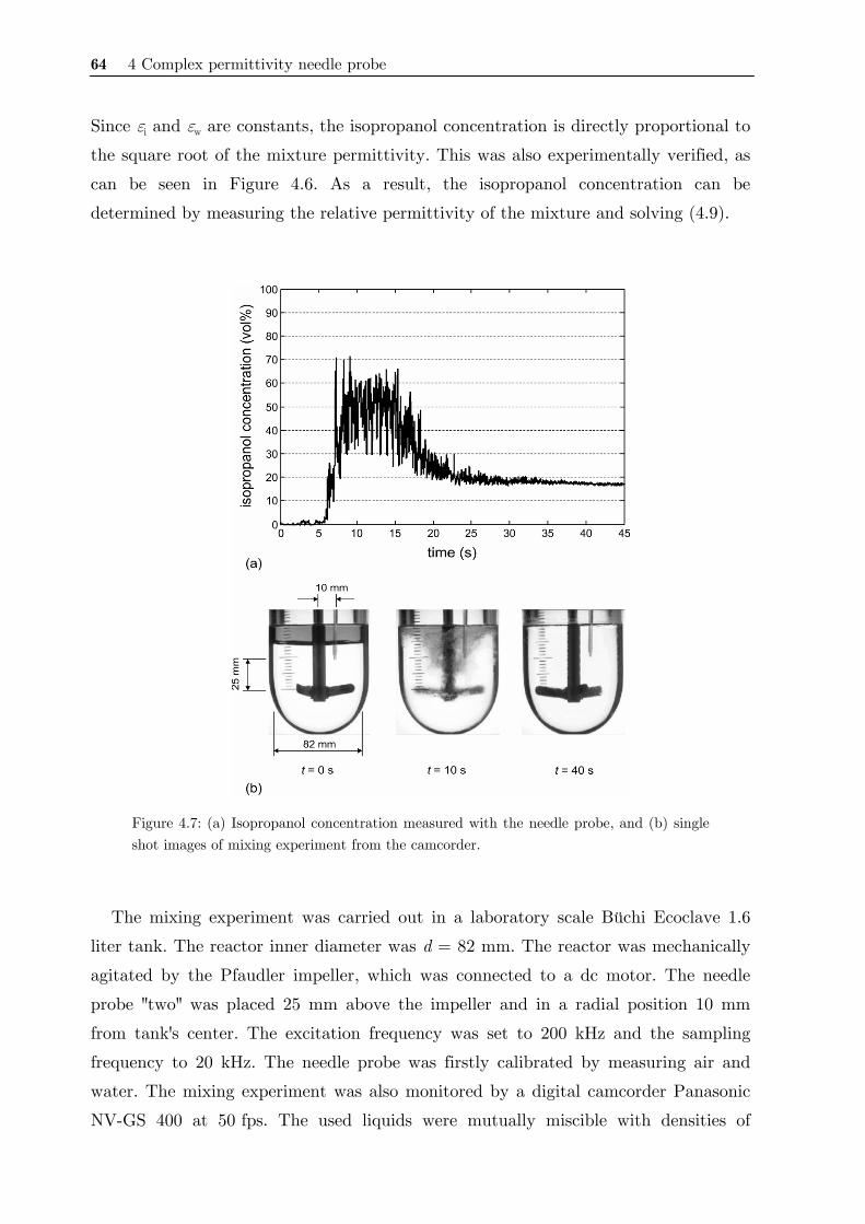
64 4 Complex permittivity needle probe
Since εi and εw are constants, the isopropanol concentration is directly proportional to
the square root of the mixture permittivity. This was also experimentally verified, as
can be seen in Figure 4.6. As a result, the isopropanol concentration can be
determined by measuring the relative permittivity of the mixture and solving (4.9).
Figure 4.7: (a) Isopropanol concentration measured with the needle probe, and (b) single shot images of mixing experiment from the camcorder.
The mixing experiment was carried out in a laboratory scale Büchi Ecoclave 1.6
liter tank. The reactor inner diameter was d = 82 mm. The reactor was mechanically
agitated by the Pfaudler impeller, which was connected to a dc motor. The needle
probe "two" was placed 25 mm above the impeller and in a radial position 10 mm
from tank's center. The excitation frequency was set to 200 kHz and the sampling
frequency to 20 kHz. The needle probe was firstly calibrated by measuring air and
water. The mixing experiment was also monitored by a digital camcorder Panasonic
NV-GS 400 at 50 fps. The used liquids were mutually miscible with densities of
4.5 Conclusions 65
998 kg/m3 for the water and 780 kg/m3 for the isopropanol. Since both substances are
transparent, the isopropanol was colored by a blue ink, in order to provide contrast
for the video visualization. The total liquid level was h = 82 mm, chosen to be close
to the commonly found in the mixing practice ratio of d/h = 1. A two layer initial
condition was obtained by first pouring 345 ml water and then 75 ml isopropanol into
the tank. The mixing process was started by rotating the impeller at 187 rpm. The
temporal evaluation of the isopropanol concentration determined by the needle probe,
which is based on permittivity measurements and calculated via (4.9), are shown in
Figure 4.7, as well as three single shot images from the camcorder.
At t = 0 the impeller started rotating. After five seconds the isopropanol
component surface reached the needle probe thus rapidly increasing the measured
concentration. A maximum concentration of about 70% is obtained between t = 5 s
and t = 15 s. From t = 15 s the isopropanol concentration started decreasing.
Complete mixing was reached 40 seconds after the impeller rotation started. The final
isopropanol concentration was measured to be 16.5% (mean value of last five
seconds), very close to the theoretical value 17.8% calculated from the initial
component volume ratio (i.e. cfinal = 75 ml / 420 ml). The camcorder images of Figure
4.7 also illustrate the mixing process: t = 0 s initial stratified condition; t = 10 s the
two components were brought into motion by the rotating impeller, the interfacial
area of both components can be well identified; and t = 40 s both substances are
completely mixed.
The time-resolved local concentration measurement by the needle probe can reveal
some details about the mixing behavior of two miscible liquids with different
densities. For example, the fluctuations in the concentration values suggest that the
interfacial area of both components was oscillating over the measurement point.
4.5 Conclusions
The evaluation of the sensor shows good linearity, reproducibility and adequate
accuracy when compared with reference values. For the first time the local complex
permittivity measurements of a three-phase bubbly flow have been presented. The
sensor is able to differentiate each phase by evaluating both relative permittivity and
conductivity signals.

66 4 Complex permittivity needle probe
Furthermore, the good accuracy in complex permittivity measurements enables the
sensor not only to be employed as phase discriminator but also to measure
concentration of a two-component mixing.
The probe was also evaluated to measure local concentration of a mixing process
on a laboratory scale stirred tank. The detailed analysis of such measurements can
reveal more details about the mixing process and should be further investigated.
Finally, all these characteristics combined with the high-speed measurement
system feature make the needle probe system a suitable new tool to investigate
dynamic phenomena in multiphase flow.
67
5 Capacitance wire-mesh sensor
Wire-mesh sensors are able to image multiphase flows with high
spatial and temporal resolution. A novel wire-mesh sensor based on
capacitance (permittivity) measurements is presented in this chapter.
The developed sensor can be used to measure transient phase fraction
distributions in a flow cross section, such as in a pipe or another
vessel by discriminating fluids with different permittivity values.
5.1 Introduction
Several measuring techniques for the investigation of flow phenomena have been
proposed and investigated in the past (see section 2.2). Especially the use of
tomography visualization techniques are of great interest since these are non-invasive
and enable the visualization of phase fractions distributions in multiphase flows.
However, currently all of the existing technical solutions have considerable
drawbacks. Thus, x-ray, γ-ray, PET and MRI scanners yet do not have sufficient
time resolution either due to the requirement for rotating parts in the scanners or
limits in radiation power. Electrical tomography techniques (e.g. ERT, ECT) achieve
high time resolution but have intrinsically low spatial resolution due to the applied
soft fields. Optical and ultrasound tomography are only suited for flows with low void
fraction.
The conductivity wire-mesh sensor, which was first proposed for high-speed liquid
flow measurements by Prasser et al. (1998), is a hybrid solution in between intrusive
probe and tomographic cross-sectional imaging (section 2.2.3). Void fraction and
bubble size measurements with temporal resolution of up to 10 000 frames per second
(fps) and spatial resolution of up to 2 mm have been achieved (Prasser et al. 2002b).
Nevertheless, current wire-mesh systems are only suitable to investigate flows where
one phase is a conductive medium, typically with electrical conductivity of at least

68 5 Capacitance wire-mesh sensor
0.5 μS/cm. Therefore, wire-mesh sensors have almost exclusively been used for the
investigation of air-water or steam-water systems.
Figure 5.1: Photo of the experimental wire-mesh sensors used in this work. (a) Laboratory sensor with 16 × 16 configuration and (b) 24 × 24 wire-mesh sensor for pipe flow investigation.
In the chemical processing industry the occurrence of non-conducting fluids such as
oil or organic liquids are common, for instance in distillation columns or in pipelines.
In those applications the measurements with current wire-mesh sensor would fail.
However, this limitation can be overcome by performing permittivity (or capacitance)
measurements instead of conductivity measurements (Da Silva et al. 2007b). In this
way, a great number of new application fields of wire-mesh sensors can be explored.
This chapter presents design, evaluation and application of a novel wire-mesh
sensor system based on permittivity (capacitance) measurements which has been
applied to investigate multiphase flows involving non-conducting fluids. The
evaluation of sensor includes simulation analysis of electrical field distribution
(section 5.3) and experimental tests regarding metrological quantities (section 5.4).
Some flow applications of the sensor are described in section 5.5.
5.2 System description
5.2.1 Sensor and measuring electronics
The prototype sensor used for experimental verification of the capacitance
measurement technique has the same design as a conductivity wire-mesh sensor
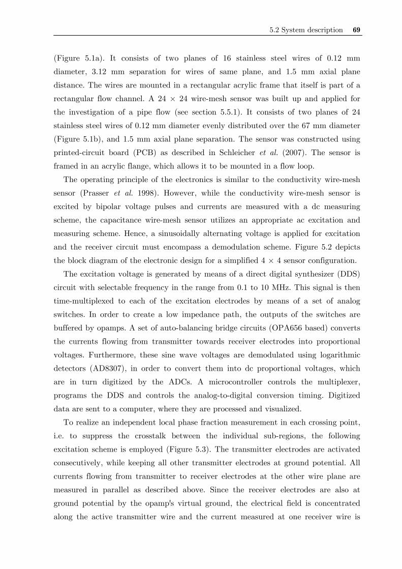
5.2 System description 69
(Figure 5.1a). It consists of two planes of 16 stainless steel wires of 0.12 mm
diameter, 3.12 mm separation for wires of same plane, and 1.5 mm axial plane
distance. The wires are mounted in a rectangular acrylic frame that itself is part of a
rectangular flow channel. A 24 × 24 wire-mesh sensor was built up and applied for
the investigation of a pipe flow (see section 5.5.1). It consists of two planes of 24
stainless steel wires of 0.12 mm diameter evenly distributed over the 67 mm diameter
(Figure 5.1b), and 1.5 mm axial plane separation. The sensor was constructed using
printed-circuit board (PCB) as described in Schleicher et al. (2007). The sensor is
framed in an acrylic flange, which allows it to be mounted in a flow loop.
The operating principle of the electronics is similar to the conductivity wire-mesh
sensor (Prasser et al. 1998). However, while the conductivity wire-mesh sensor is
excited by bipolar voltage pulses and currents are measured with a dc measuring
scheme, the capacitance wire-mesh sensor utilizes an appropriate ac excitation and
measuring scheme. Hence, a sinusoidally alternating voltage is applied for excitation
and the receiver circuit must encompass a demodulation scheme. Figure 5.2 depicts
the block diagram of the electronic design for a simplified 4 × 4 sensor configuration.
The excitation voltage is generated by means of a direct digital synthesizer (DDS)
circuit with selectable frequency in the range from 0.1 to 10 MHz. This signal is then
time-multiplexed to each of the excitation electrodes by means of a set of analog
switches. In order to create a low impedance path, the outputs of the switches are
buffered by opamps. A set of auto-balancing bridge circuits (OPA656 based) converts
the currents flowing from transmitter towards receiver electrodes into proportional
voltages. Furthermore, these sine wave voltages are demodulated using logarithmic
detectors (AD8307), in order to convert them into dc proportional voltages, which
are in turn digitized by the ADCs. A microcontroller controls the multiplexer,
programs the DDS and controls the analog-to-digital conversion timing. Digitized
data are sent to a computer, where they are processed and visualized.
To realize an independent local phase fraction measurement in each crossing point,
i.e. to suppress the crosstalk between the individual sub-regions, the following
excitation scheme is employed (Figure 5.3). The transmitter electrodes are activated
consecutively, while keeping all other transmitter electrodes at ground potential. All
currents flowing from transmitter to receiver electrodes at the other wire plane are
measured in parallel as described above. Since the receiver electrodes are also at
ground potential by the opamp's virtual ground, the electrical field is concentrated
along the active transmitter wire and the current measured at one receiver wire is
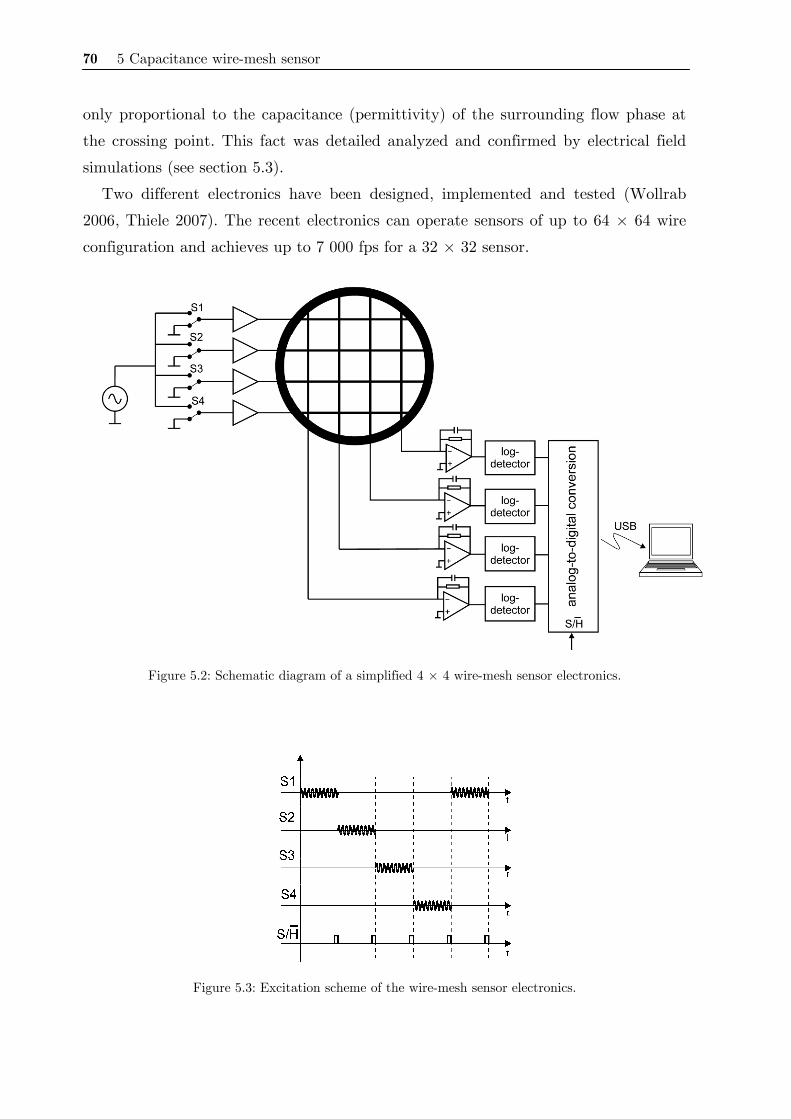
70 5 Capacitance wire-mesh sensor
only proportional to the capacitance (permittivity) of the surrounding flow phase at
the crossing point. This fact was detailed analyzed and confirmed by electrical field
simulations (see section 5.3).
Two different electronics have been designed, implemented and tested (Wollrab
2006, Thiele 2007). The recent electronics can operate sensors of up to 64 × 64 wire
configuration and achieves up to 7 000 fps for a 32 × 32 sensor.
Figure 5.2: Schematic diagram of a simplified 4 × 4 wire-mesh sensor electronics.
Figure 5.3: Excitation scheme of the wire-mesh sensor electronics.
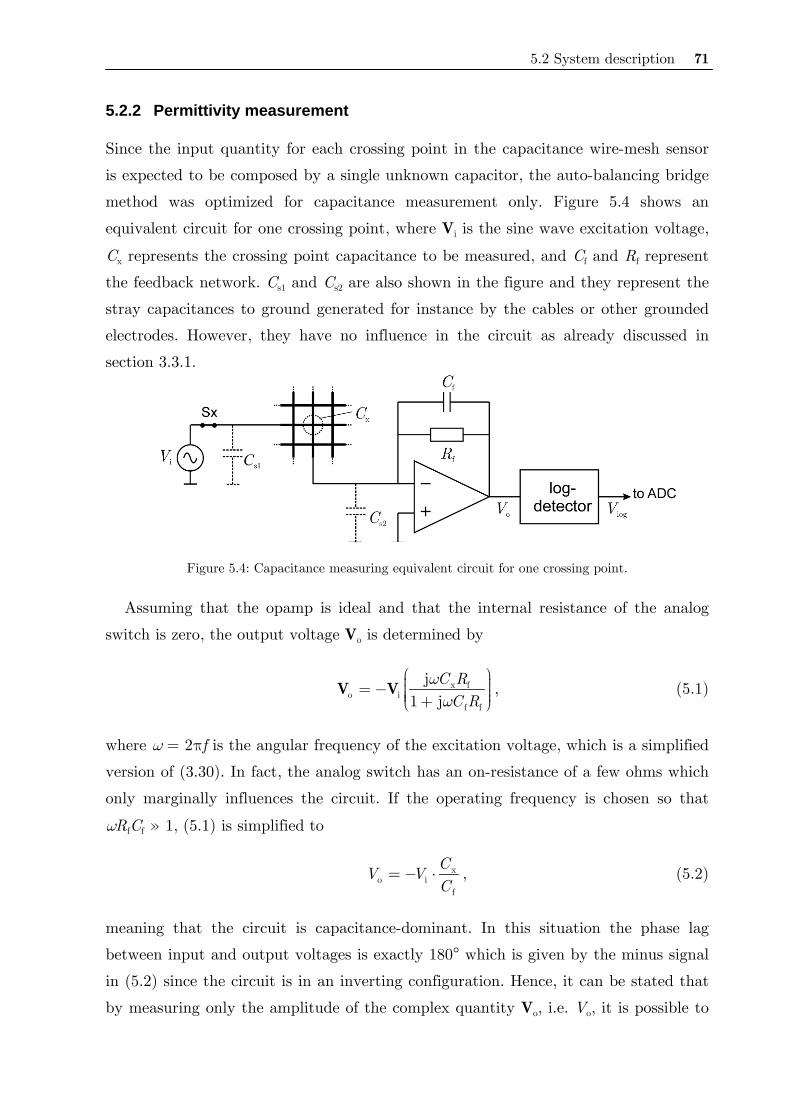
5.2 System description 71
5.2.2 Permittivity measurement
Since the input quantity for each crossing point in the capacitance wire-mesh sensor
is expected to be composed by a single unknown capacitor, the auto-balancing bridge
method was optimized for capacitance measurement only. Figure 5.4 shows an
equivalent circuit for one crossing point, where Vi is the sine wave excitation voltage,
Cx represents the crossing point capacitance to be measured, and Cf and Rf represent
the feedback network. Cs1 and Cs2 are also shown in the figure and they represent the
stray capacitances to ground generated for instance by the cables or other grounded
electrodes. However, they have no influence in the circuit as already discussed in
section 3.3.1.
Figure 5.4: Capacitance measuring equivalent circuit for one crossing point.
Assuming that the opamp is ideal and that the internal resistance of the analog
switch is zero, the output voltage Vo is determined by
x fo i
f f
j1 j
C RC R
ωω
⎛ ⎞⎟⎜ ⎟= − ⎜ ⎟⎜ ⎟⎜ +⎝ ⎠V V , (5.1)
where ω = 2πf is the angular frequency of the excitation voltage, which is a simplified
version of (3.30). In fact, the analog switch has an on-resistance of a few ohms which
only marginally influences the circuit. If the operating frequency is chosen so that
ωRfCf » 1, (5.1) is simplified to
xo i
f
CV VC
= − ⋅ , (5.2)
meaning that the circuit is capacitance-dominant. In this situation the phase lag
between input and output voltages is exactly 180° which is given by the minus signal
in (5.2) since the circuit is in an inverting configuration. Hence, it can be stated that
by measuring only the amplitude of the complex quantity Vo, i.e. Vo, it is possible to
72 5 Capacitance wire-mesh sensor
determine the capacitance value of the fluid phase at the crossing point. For the
feedback network Rf = 1 MΩ and Cf = 1 pF were employed, and a typical excitation
frequency of 5 MHz was chosen. In this way, ωRfCf = 31 and (5.2) is a good
approximation. Nevertheless, (5.1) may also be used if more accurate values are
needed.
The sinusoidal alternating voltage Vo has to be demodulated so that it can be
digitized, i.e. the ac signal has to be converted into a proportional dc one. Since a
high signal dynamics from measurements on different substances are expected, a
logarithmic detector scheme for the demodulation of the ac signal was chosen. Even
very small changes in the capacitance Cx (and consequently in Vo) can be measured
by maintaining a fast response time. The log-detector AD8307 output is in the form
olog a
b
ln VV VV
⎛ ⎞⎟⎜ ⎟= ⋅ ⎜ ⎟⎜ ⎟⎜⎝ ⎠, (5.3)
where Va and Vb are constants of the integrated circuit. Taking (5.2) into (5.3) and
remembering (3.22) that Cx is directly proportional to permittivity εx of the substance
in the crossing point, it results in
( )log xlnV a bε= ⋅ + , (5.4)
where a and b are constants that encompass the geometry factor kg of a crossing
point, Rf and Cf, the log-detector constants, f the measuring frequency and Vi the
input voltage.
The acquired voltages Vlog for all crossing points are saved in an Nx × Ny × Nt
data matrix in computer memory, where Nx and Ny denote the number of sender and
receiver electrodes and Nt the number of acquired time steps. The data are related to
the permittivity distribution over the cross section via (5.4), but evidently this raw
data need further processing to discriminate phases or determine absolute capacitance
values. Due to differences in the electrical characteristics of the individual
components, for instance resistor tolerances, opamp gains etc, there is a considerable
intrinsic variance in the measured values of each crossing point. In order to
compensate this variance, a calibration routine is required, which is described as
follows.
First, the sensor is measured with a substance of low permittivity εL covering the
whole sensor giving a reference data matrix
5.2 System description 73
t 1
Llog
0t
1( , ) ( , , )N
k
V i j V i j kN
−
=
= ∑ , (5.5)
which is an average of the raw data over a sufficient temporal range. Here, i and j
denote the wire indices and k the temporal sampling point index.
The procedure is then repeated with the entire cross section of the sensor covered
with another substance having a higher permittivity εH, which gives another reference
data matrix denoted by HV . In this fashion, applying equation (5.4) for both
calibration data matrixes HV and LV it is possible to calculate the constants of (5.4)
for every crossing point as
( ) ( )
H L
H L
( , ) ( , )( , )ln ln
V i j V i ja i jε ε
−=−
(5.6)
( ) ( )( ) ( )
L HH L
H L
( , )ln ( , )ln( , )
ln lnV i j V i j
b i jε εε ε
−=
−. (5.7)
Finally, the permittivity distribution over the cross-section can be determined by
inverting (5.4) and applying it for every crossing point, thus
log( , , ) ( , )( , , ) exp
( , )V i j k b i j
i j ka i j
ε⎛ ⎞− ⎟⎜ ⎟= ⎜ ⎟⎜ ⎟⎜⎝ ⎠
. (5.8)
In the case that the lower permittivity reference substance is air which has ε = 1,
(5.8) is simplified to
( )L
logHH L
( , , )( , , ) exp ln
V i j k Vi j k
V Vε ε
⎛ ⎞− ⎟⎜ ⎟= ⎜ ⎟⎜ ⎟⎜ −⎝ ⎠. (5.9)
For the determination of the local phase fraction distribution ( , , )i j kα , a linear
relationship between the measured permittivity and the phase fraction is assumed
H
H L
( , ) ( , , )( , , )( , ) ( , )i j i j ki j ki j i j
ε εαε ε
−=−
. (5.10)
The assumption of a linear dependence between the local phase fraction level and
the crossing point permittivity is obviously a simplification. It basically models the
crossing points as a parallel plate capacitor with a homogenous phase distribution
between capacitor's plates. An analogous assumption has been successfully employed
for conductivity wire-mesh sensors (Prasser et al. 1998) and for ECT systems
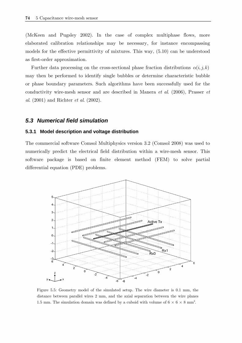
74 5 Capacitance wire-mesh sensor
(McKeen and Pugsley 2002). In the case of complex multiphase flows, more
elaborated calibration relationships may be necessary, for instance encompassing
models for the effective permittivity of mixtures. This way, (5.10) can be understood
as first-order approximation.
Further data processing on the cross-sectional phase fraction distributions ( , , )i j kα
may then be performed to identify single bubbles or determine characteristic bubble
or phase boundary parameters. Such algorithms have been successfully used for the
conductivity wire-mesh sensor and are described in Manera et al. (2006), Prasser et
al. (2001) and Richter et al. (2002).
5.3 Numerical field simulation
5.3.1 Model description and voltage distribution
The commercial software Comsol Multiphysics version 3.2 (Comsol 2008) was used to
numerically predict the electrical field distribution within a wire-mesh sensor. This
software package is based on finite element method (FEM) to solve partial
differential equation (PDE) problems.
Figure 5.5: Geometry model of the simulated setup. The wire diameter is 0.1 mm, the distance between parallel wires 2 mm, and the axial separation between the wire planes 1.5 mm. The simulation domain was defined by a cuboid with volume of 6 × 6 × 8 mm3.
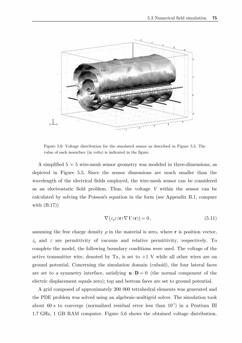
5.3 Numerical field simulation 75
Figure 5.6: Voltage distribution for the simulated sensor as described in Figure 5.5. The value of each isosurface (in volts) is indicated in the figure.
A simplified 5 × 5 wire-mesh sensor geometry was modeled in three-dimensions, as
depicted in Figure 5.5. Since the sensor dimensions are much smaller than the
wavelength of the electrical fields employed, the wire-mesh sensor can be considered
as an electrostatic field problem. Thus, the voltage V within the sensor can be
calculated by solving the Poisson's equation in the form (see Appendix B.1, compare
with (B.17))
( ) ( )( )0 0Vε ε∇ ∇ =r r , (5.11)
assuming the free charge density ρ in the material is zero, where r is position vector,
ε0 and ε are permittivity of vacuum and relative permittivity, respectively. To
complete the model, the following boundary conditions were used. The voltage of the
active transmitter wire, denoted by Tx, is set to +1 V while all other wires are on
ground potential. Concerning the simulation domain (cuboid), the four lateral faces
are set to a symmetry interface, satisfying 0⋅ =n D (the normal component of the
electric displacement equals zero); top and bottom faces are set to ground potential.
A grid composed of approximately 200 000 tetrahedral elements was generated and
the PDE problem was solved using an algebraic-multigrid solver. The simulation took
about 60 s to converge (normalized residual error less than 10-7) in a Pentium III
1.7 GHz, 1 GB RAM computer. Figure 5.6 shows the obtained voltage distribution.
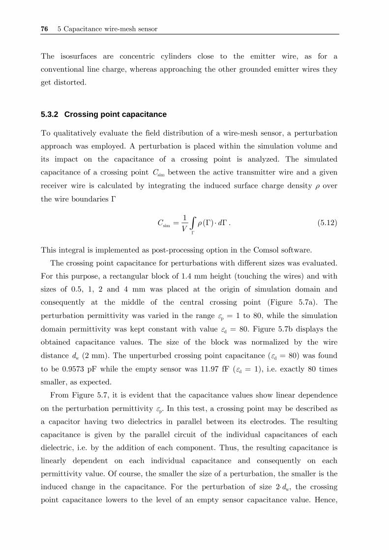
76 5 Capacitance wire-mesh sensor
The isosurfaces are concentric cylinders close to the emitter wire, as for a
conventional line charge, whereas approaching the other grounded emitter wires they
get distorted.
5.3.2 Crossing point capacitance
To qualitatively evaluate the field distribution of a wire-mesh sensor, a perturbation
approach was employed. A perturbation is placed within the simulation volume and
its impact on the capacitance of a crossing point is analyzed. The simulated
capacitance of a crossing point Csim between the active transmitter wire and a given
receiver wire is calculated by integrating the induced surface charge density ρ over
the wire boundaries Γ
( )sim1C dV
ρΓ
= Γ ⋅ Γ∫ . (5.12)
This integral is implemented as post-processing option in the Comsol software.
The crossing point capacitance for perturbations with different sizes was evaluated.
For this purpose, a rectangular block of 1.4 mm height (touching the wires) and with
sizes of 0.5, 1, 2 and 4 mm was placed at the origin of simulation domain and
consequently at the middle of the central crossing point (Figure 5.7a). The
perturbation permittivity was varied in the range εp = 1 to 80, while the simulation
domain permittivity was kept constant with value εd = 80. Figure 5.7b displays the
obtained capacitance values. The size of the block was normalized by the wire
distance dw (2 mm). The unperturbed crossing point capacitance (εd = 80) was found
to be 0.9573 pF while the empty sensor was 11.97 fF (εd = 1), i.e. exactly 80 times
smaller, as expected.
From Figure 5.7, it is evident that the capacitance values show linear dependence
on the perturbation permittivity εp. In this test, a crossing point may be described as
a capacitor having two dielectrics in parallel between its electrodes. The resulting
capacitance is given by the parallel circuit of the individual capacitances of each
dielectric, i.e. by the addition of each component. Thus, the resulting capacitance is
linearly dependent on each individual capacitance and consequently on each
permittivity value. Of course, the smaller the size of a perturbation, the smaller is the
induced change in the capacitance. For the perturbation of size 2⋅dw, the crossing
point capacitance lowers to the level of an empty sensor capacitance value. Hence,
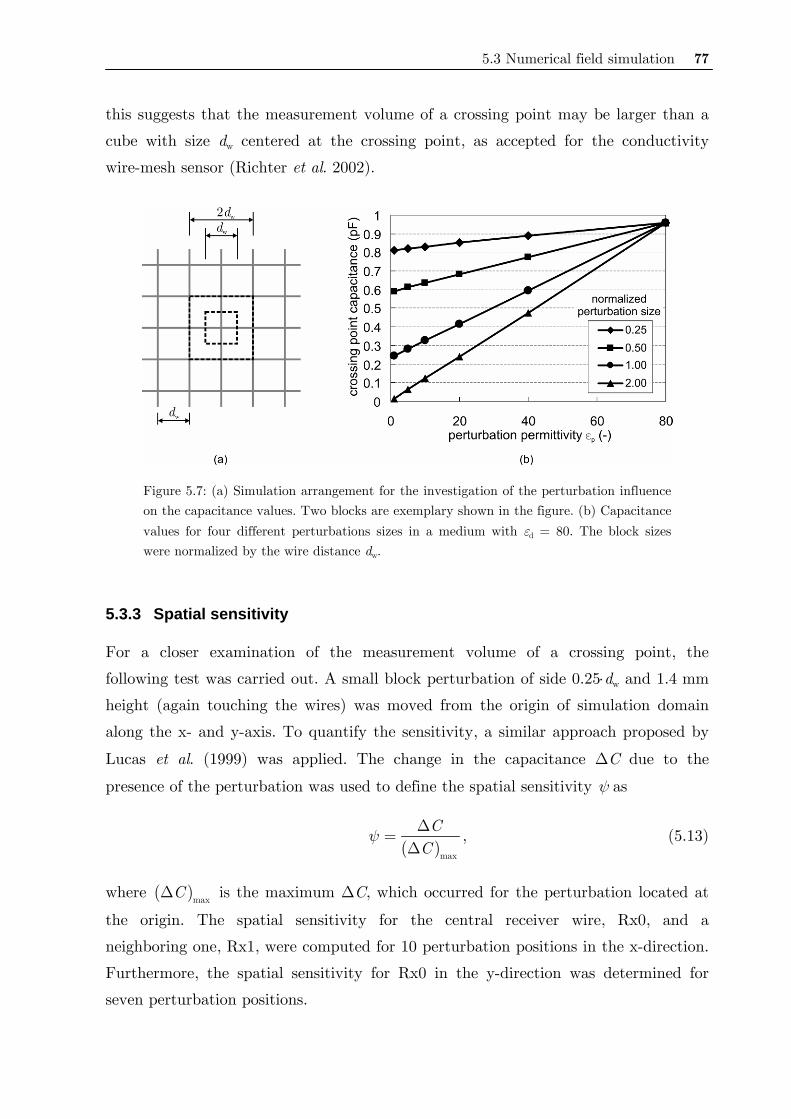
5.3 Numerical field simulation 77
this suggests that the measurement volume of a crossing point may be larger than a
cube with size dw centered at the crossing point, as accepted for the conductivity
wire-mesh sensor (Richter et al. 2002).
Figure 5.7: (a) Simulation arrangement for the investigation of the perturbation influence on the capacitance values. Two blocks are exemplary shown in the figure. (b) Capacitance values for four different perturbations sizes in a medium with εd = 80. The block sizes were normalized by the wire distance dw.
5.3.3 Spatial sensitivity
For a closer examination of the measurement volume of a crossing point, the
following test was carried out. A small block perturbation of side 0.25⋅dw and 1.4 mm
height (again touching the wires) was moved from the origin of simulation domain
along the x- and y-axis. To quantify the sensitivity, a similar approach proposed by
Lucas et al. (1999) was applied. The change in the capacitance ΔC due to the
presence of the perturbation was used to define the spatial sensitivity ψ as
( )max
CC
ψ Δ=Δ
, (5.13)
where ( )maxCΔ is the maximum ΔC, which occurred for the perturbation located at
the origin. The spatial sensitivity for the central receiver wire, Rx0, and a
neighboring one, Rx1, were computed for 10 perturbation positions in the x-direction.
Furthermore, the spatial sensitivity for Rx0 in the y-direction was determined for
seven perturbation positions.
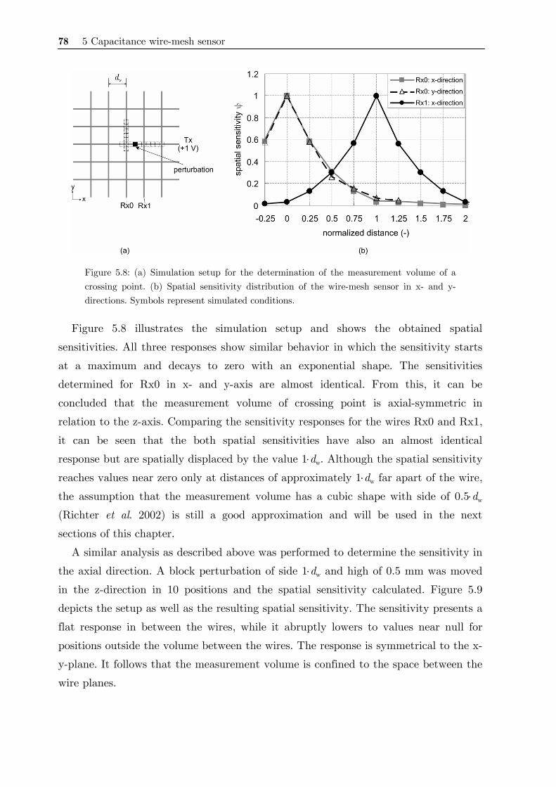
78 5 Capacitance wire-mesh sensor
Figure 5.8: (a) Simulation setup for the determination of the measurement volume of a crossing point. (b) Spatial sensitivity distribution of the wire-mesh sensor in x- and y-directions. Symbols represent simulated conditions.
Figure 5.8 illustrates the simulation setup and shows the obtained spatial
sensitivities. All three responses show similar behavior in which the sensitivity starts
at a maximum and decays to zero with an exponential shape. The sensitivities
determined for Rx0 in x- and y-axis are almost identical. From this, it can be
concluded that the measurement volume of crossing point is axial-symmetric in
relation to the z-axis. Comparing the sensitivity responses for the wires Rx0 and Rx1,
it can be seen that the both spatial sensitivities have also an almost identical
response but are spatially displaced by the value 1⋅dw. Although the spatial sensitivity
reaches values near zero only at distances of approximately 1⋅dw far apart of the wire,
the assumption that the measurement volume has a cubic shape with side of 0.5⋅dw
(Richter et al. 2002) is still a good approximation and will be used in the next
sections of this chapter.
A similar analysis as described above was performed to determine the sensitivity in
the axial direction. A block perturbation of side 1⋅dw and high of 0.5 mm was moved
in the z-direction in 10 positions and the spatial sensitivity calculated. Figure 5.9
depicts the setup as well as the resulting spatial sensitivity. The sensitivity presents a
flat response in between the wires, while it abruptly lowers to values near null for
positions outside the volume between the wires. The response is symmetrical to the x-
y-plane. It follows that the measurement volume is confined to the space between the
wire planes.
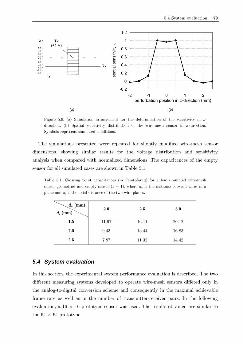
5.4 System evaluation 79
Figure 5.9: (a) Simulation arrangement for the determination of the sensitivity in z-direction. (b) Spatial sensitivity distribution of the wire-mesh sensor in z-direction. Symbols represent simulated conditions.
The simulations presented were repeated for slightly modified wire-mesh sensor
dimensions, showing similar results for the voltage distribution and sensitivity
analysis when compared with normalized dimensions. The capacitances of the empty
sensor for all simulated cases are shown in Table 5.1.
Table 5.1: Crossing point capacitances (in Femtofarad) for a few simulated wire-mesh sensor geometries and empty sensor (ε = 1), where dw is the distance between wires in a plane and dz is the axial distance of the two wire planes.
dw (mm)
dz (mm) 2.0 2.5 3.0
1.5 11.97 16.11 20.12
2.0 9.43 13.44 16.83
2.5 7.87 11.32 14.42
5.4 System evaluation
In this section, the experimental system performance evaluation is described. The two
different measuring systems developed to operate wire-mesh sensors differed only in
the analog-to-digital conversion scheme and consequently in the maximal achievable
frame rate as well as in the number of transmitter-receiver pairs. In the following
evaluation, a 16 × 16 prototype sensor was used. The results obtained are similar to
the 64 × 64 prototype.
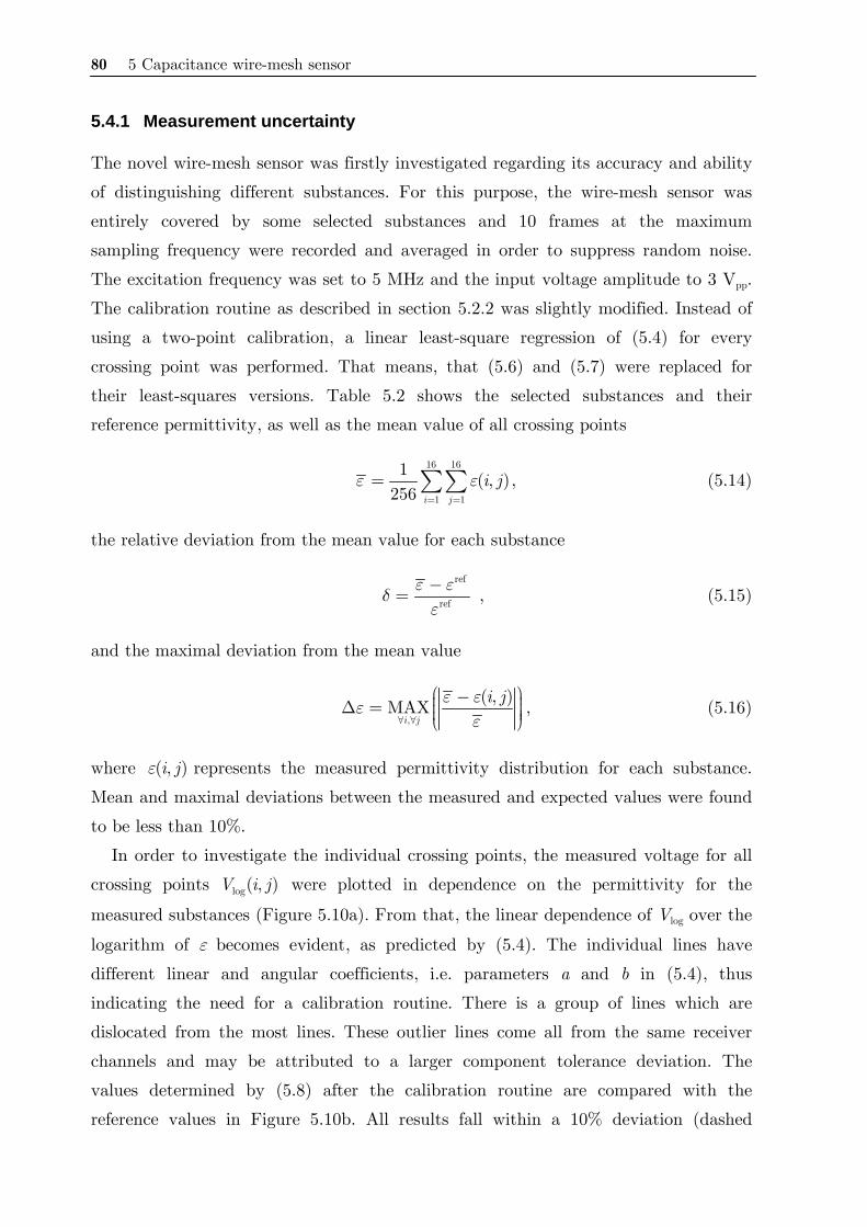
80 5 Capacitance wire-mesh sensor
5.4.1 Measurement uncertainty
The novel wire-mesh sensor was firstly investigated regarding its accuracy and ability
of distinguishing different substances. For this purpose, the wire-mesh sensor was
entirely covered by some selected substances and 10 frames at the maximum
sampling frequency were recorded and averaged in order to suppress random noise.
The excitation frequency was set to 5 MHz and the input voltage amplitude to 3 Vpp.
The calibration routine as described in section 5.2.2 was slightly modified. Instead of
using a two-point calibration, a linear least-square regression of (5.4) for every
crossing point was performed. That means, that (5.6) and (5.7) were replaced for
their least-squares versions. Table 5.2 shows the selected substances and their
reference permittivity, as well as the mean value of all crossing points
16 16
1 1
1 ( , )256 i j
i jε ε= =
= ∑∑ , (5.14)
the relative deviation from the mean value for each substance
ref
ref
ε εδε−= , (5.15)
and the maximal deviation from the mean value
,
( , )MAXi j
i jε εεε∀ ∀
⎛ ⎞− ⎟⎜Δ = ⎟⎜ ⎟⎟⎜⎝ ⎠, (5.16)
where ( , )i jε represents the measured permittivity distribution for each substance.
Mean and maximal deviations between the measured and expected values were found
to be less than 10%.
In order to investigate the individual crossing points, the measured voltage for all
crossing points log( , )V i j were plotted in dependence on the permittivity for the
measured substances (Figure 5.10a). From that, the linear dependence of Vlog over the
logarithm of ε becomes evident, as predicted by (5.4). The individual lines have
different linear and angular coefficients, i.e. parameters a and b in (5.4), thus
indicating the need for a calibration routine. There is a group of lines which are
dislocated from the most lines. These outlier lines come all from the same receiver
channels and may be attributed to a larger component tolerance deviation. The
values determined by (5.8) after the calibration routine are compared with the
reference values in Figure 5.10b. All results fall within a 10% deviation (dashed
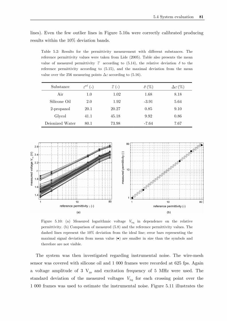
5.4 System evaluation 81
lines). Even the few outlier lines in Figure 5.10a were correctly calibrated producing
results within the 10% deviation bands.
Table 5.2: Results for the permittivity measurement with different substances. The reference permittivity values were taken from Lide (2005). Table also presents the mean value of measured permittivity ε according to (5.14), the relative deviation δ to the reference permittivity according to (5.15), and the maximal deviation from the mean value over the 256 measuring points Δε according to (5.16).
Substance εref (-) ε (-) δ (%) Δε (%)
Air 1.0 1.02 1.68 8.18
Silicone Oil 2.0 1.92 -3.91 5.64
2-propanol 20.1 20.27 0.85 9.10
Glycol 41.1 45.18 9.92 0.86
Deionized Water 80.1 73.98 -7.64 7.67
Figure 5.10: (a) Measured logarithmic voltage Vlog in dependence on the relative permittivity. (b) Comparison of measured (5.8) and the reference permittivity values. The dashed lines represent the 10% deviation from the ideal line; error bars representing the maximal signal deviation from mean value (•) are smaller in size than the symbols and therefore are not visible.
The system was then investigated regarding instrumental noise. The wire-mesh
sensor was covered with silicone oil and 1 000 frames were recorded at 625 fps. Again
a voltage amplitude of 3 Vpp and excitation frequency of 5 MHz were used. The
standard deviation of the measured voltages Vlog for each crossing point over the
1 000 frames was used to estimate the instrumental noise. Figure 5.11 illustrates the
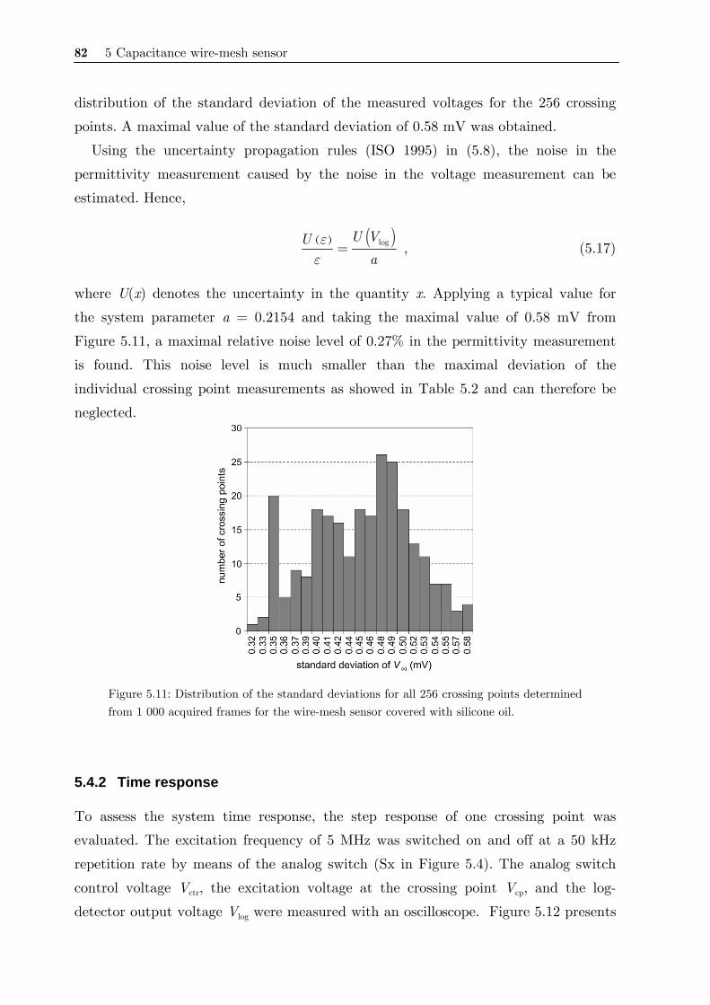
82 5 Capacitance wire-mesh sensor
distribution of the standard deviation of the measured voltages for the 256 crossing
points. A maximal value of the standard deviation of 0.58 mV was obtained.
Using the uncertainty propagation rules (ISO 1995) in (5.8), the noise in the
permittivity measurement caused by the noise in the voltage measurement can be
estimated. Hence,
( ) ( )logU VU
aεε
= , (5.17)
where U(x) denotes the uncertainty in the quantity x. Applying a typical value for
the system parameter a = 0.2154 and taking the maximal value of 0.58 mV from
Figure 5.11, a maximal relative noise level of 0.27% in the permittivity measurement
is found. This noise level is much smaller than the maximal deviation of the
individual crossing point measurements as showed in Table 5.2 and can therefore be
neglected.
Figure 5.11: Distribution of the standard deviations for all 256 crossing points determined from 1 000 acquired frames for the wire-mesh sensor covered with silicone oil.
5.4.2 Time response
To assess the system time response, the step response of one crossing point was
evaluated. The excitation frequency of 5 MHz was switched on and off at a 50 kHz
repetition rate by means of the analog switch (Sx in Figure 5.4). The analog switch
control voltage Vctr, the excitation voltage at the crossing point Vcp, and the log-
detector output voltage Vlog were measured with an oscilloscope. Figure 5.12 presents

5.4 System evaluation 83
the results showing normalized voltages. It is clear that the time response of the
circuit is determined by the receiver circuit response. While the voltage Vcp responds
within a few nanoseconds, Vlog presents typical exponential first-order system
response. The measured settling times for 1% error in Vlog were 4.13 μs and 4.40 μs
for turn on and turn off, respectively. These values are slightly larger than the ones
specified in the log-detector data sheet, which is explained by the fact that a larger
capacitor value (68 pF instead of 2 pF recommended in the data sheet) was used at
the log-detector output to reduce the output signal ripple. If required, the time
response might thus still be improved by lowering the capacitor value, but on cost of
increasing the noise level and thus the uncertainty in the measurements. The
measured time response corresponds to a maximal sampling frequency of 225 kHz for
the analogue-digital conversion and thus gives a maximal frame rate of 14 063 fps for
the actual 16 × 16 sensor configuration.
Figure 5.12: Step response of the receiver circuit showing the normalized analogue switch control voltage Vctr, the excitation voltage Vcp, and the log-detector output voltage Vlog.
5.4.3 Comparison with conductivity wire-mesh sensor
In order to compare the image produced by the novel capacitance wire-mesh with a
standard conductivity wire-mesh sensor, the following experiment was carried out.
Since water is a conducting substance it can be measured by both conductivity and
capacitance wire-mesh sensors and was therefore chosen.
The flow channel with integrated sensor was filled with water (electrical
conductivity σ = 2 μS/cm), placed in the horizontal position and rotated 45°. In this

84 5 Capacitance wire-mesh sensor
way, a well-defined planar phase boundary imitating a stratified two-phase flow is
realized. Figure 5.13a presents the cross-sectional images generated by both systems,
where 10 frames were acquired at 625 fps and averaged. In Figure 5.13b the lines of
equal void fraction α are shown, which were calculated by interpolating the measured
values at the crossing points. These lines represent the interface between the two
phases. The agreement between the images obtained with both systems as well the
lines of equal void fraction are very good. The figures also illustrate the suppression
of crosstalk between the individual crossing points. The presence of crosstalk would
have caused a blurring effect in the image and hence a distortion in the line of equal
void fraction. The water-air interface would not have been correctly represented. In
fact, the accuracy of the detection of the interfacial area corresponds to the size of
one mesh of wires, i.e. 3.12 mm for this sensor. In this way, the image produced by
the capacitance wire-mesh sensor (as well as the conductivity sensor) is free of
crosstalk artifacts.
Figure 5.13: (a) Cross-sectional images obtained with the capacitance and conductivity wire-mesh sensors when measuring a planar phase boundary. The gray scale represents the void fraction α. (b) Comparison of the lines of equal void fraction for three selected values (α = 0.25, 0.50, and 0.75). The lines were calculated by interpolating the measured values at the crossing points.
5.4 System evaluation 85
5.4.4 Influence of liquid conductivity
Although the circuit of the capacitance wire-mesh sensor was conceived and
implemented to measure capacitances, the influence of liquid conductivity, i.e. the
resistive part of impedance, on the auto-balancing circuit was investigated. In this
way, as described in section 3.1.2, the unknown impedance of a crossing point for a
lossy dielectric is formed by a capacitor (linked with fluid permittivity) and a resistor
(linked with fluid conductivity).
The rectangular cross-section wire-mesh sensor (Figure 5.1a) was filled with water
of increasing conductivity values which was obtained by the controlled addition of
sodium chloride. The reference conductivity was monitored with a conductivity meter
Cond 330i (WTW GmbH, Germany, 0.5% measurement uncertainty). For each
reference conductivity value, 10 frames were acquired at 625 fps and averaged. Figure
5.14a shows the measured Vlog voltages for the conductivity values varying from 1 to
104 μS/cm (or 10−4 to 1 S/m). The lowest investigated value of 1 μS/cm represents
deionized water. Tap water has a conductivity of about 400 μS/cm. The highest
value measured (104 μS/cm) corresponds approximately to sea water with a salinity
of 5.6 g/l at 25 °C and 105 Pa (Perkins and Lewis 1980).
Figure 5.14 shows the measured voltage for different conductivity values of water
for one exemplary crossing point. Similar behavior was found for the other crossing
points. Basically, two regions can be identified. For conductivity values of up to
100 μS/cm, the measured voltages Vlog are constant; meaning that the conductivity
does not play any role, i.e the circuit is capacitance-dominant. For conductivity
values higher than 100 μS/cm, the measured voltage increases with increasing
conductivity. In this second region the resistive part of the impedance starts
influencing the measurement. It is predicted that at a certain point the circuit
becomes resistance dominant and the response of Vlog turns linearly dependent on the
conductivity.
To demonstrate the above described behavior a closer analysis was performed.
Since the measured quantity is now complex, the relationship governing the circuit
output voltage must be revised. In the circuit of Figure 5.4, the logarithmic detector
measures the amplitude of the sine wave voltage Vo disregarding its phase value, thus
(5.4) may be written considering the modulus of the complex permittivity of a
crossing point
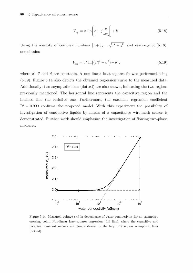
86 5 Capacitance wire-mesh sensor
log0
lnV a j bσεωε
⎛ ⎞⎟⎜ ⎟= ⋅ − +⎜ ⎟⎜ ⎟⎟⎜⎝ ⎠. (5.18)
Using the identity of complex numbers 2 2x jy x y+ = + and rearranging (5.18),
one obtains
( )( )2 2log ' ln ' 'V a c bσ= ⋅ + + , (5.19)
where a', b' and c' are constants. A non-linear least-squares fit was performed using
(5.19). Figure 5.14 also depicts the obtained regression curve to the measured data.
Additionally, two asymptotic lines (dotted) are also shown, indicating the two regions
previously mentioned. The horizontal line represents the capacitive region and the
inclined line the resistive one. Furthermore, the excellent regression coefficient
R2 = 0.999 confirms the proposed model. With this experiment the possibility of
investigation of conductive liquids by means of a capacitance wire-mesh sensor is
demonstrated. Further work should emphasize the investigation of flowing two-phase
mixtures.
Figure 5.14: Measured voltage (×) in dependence of water conductivity for an exemplary crossing point. Non-linear least-squares regression (full line), where the capacitive and resistive dominant regions are clearly shown by the help of the two asymptotic lines (dotted).
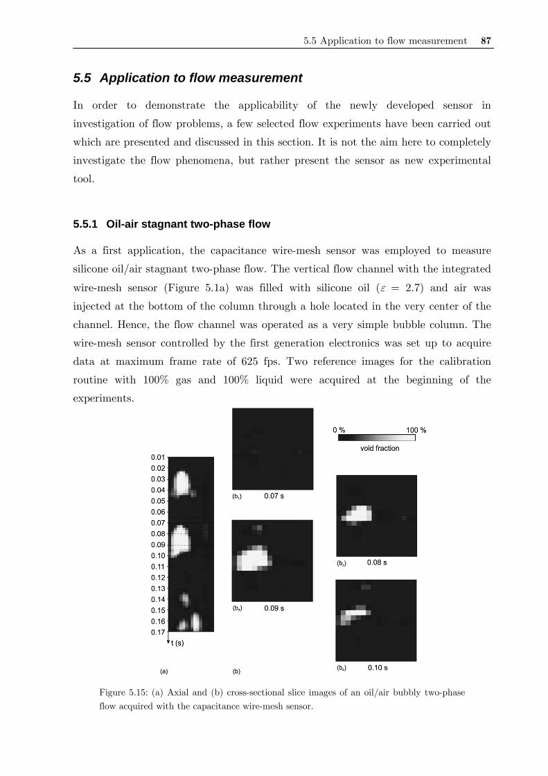
5.5 Application to flow measurement 87
5.5 Application to flow measurement
In order to demonstrate the applicability of the newly developed sensor in
investigation of flow problems, a few selected flow experiments have been carried out
which are presented and discussed in this section. It is not the aim here to completely
investigate the flow phenomena, but rather present the sensor as new experimental
tool.
5.5.1 Oil-air stagnant two-phase flow
As a first application, the capacitance wire-mesh sensor was employed to measure
silicone oil/air stagnant two-phase flow. The vertical flow channel with the integrated
wire-mesh sensor (Figure 5.1a) was filled with silicone oil (ε = 2.7) and air was
injected at the bottom of the column through a hole located in the very center of the
channel. Hence, the flow channel was operated as a very simple bubble column. The
wire-mesh sensor controlled by the first generation electronics was set up to acquire
data at maximum frame rate of 625 fps. Two reference images for the calibration
routine with 100% gas and 100% liquid were acquired at the beginning of the
experiments.
Figure 5.15: (a) Axial and (b) cross-sectional slice images of an oil/air bubbly two-phase flow acquired with the capacitance wire-mesh sensor.
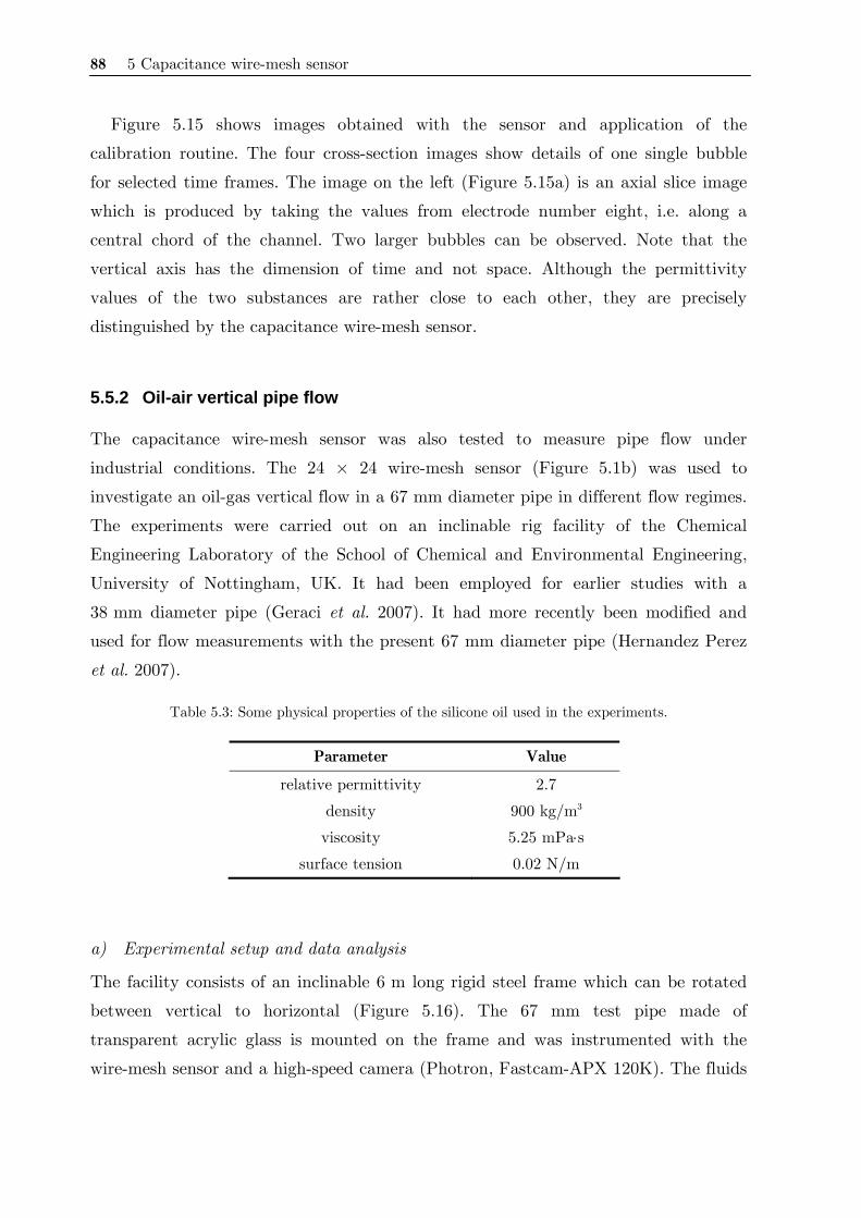
88 5 Capacitance wire-mesh sensor
Figure 5.15 shows images obtained with the sensor and application of the
calibration routine. The four cross-section images show details of one single bubble
for selected time frames. The image on the left (Figure 5.15a) is an axial slice image
which is produced by taking the values from electrode number eight, i.e. along a
central chord of the channel. Two larger bubbles can be observed. Note that the
vertical axis has the dimension of time and not space. Although the permittivity
values of the two substances are rather close to each other, they are precisely
distinguished by the capacitance wire-mesh sensor.
5.5.2 Oil-air vertical pipe flow
The capacitance wire-mesh sensor was also tested to measure pipe flow under
industrial conditions. The 24 × 24 wire-mesh sensor (Figure 5.1b) was used to
investigate an oil-gas vertical flow in a 67 mm diameter pipe in different flow regimes.
The experiments were carried out on an inclinable rig facility of the Chemical
Engineering Laboratory of the School of Chemical and Environmental Engineering,
University of Nottingham, UK. It had been employed for earlier studies with a
38 mm diameter pipe (Geraci et al. 2007). It had more recently been modified and
used for flow measurements with the present 67 mm diameter pipe (Hernandez Perez
et al. 2007).
Table 5.3: Some physical properties of the silicone oil used in the experiments.
Parameter Value
relative permittivity 2.7
density 900 kg/m3
viscosity 5.25 mPa⋅s
surface tension 0.02 N/m
a) Experimental setup and data analysis
The facility consists of an inclinable 6 m long rigid steel frame which can be rotated
between vertical to horizontal (Figure 5.16). The 67 mm test pipe made of
transparent acrylic glass is mounted on the frame and was instrumented with the
wire-mesh sensor and a high-speed camera (Photron, Fastcam-APX 120K). The fluids
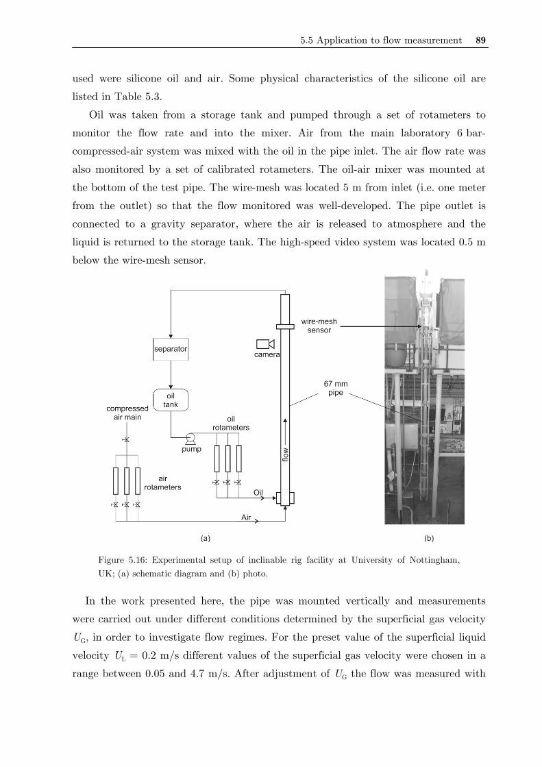
5.5 Application to flow measurement 89
used were silicone oil and air. Some physical characteristics of the silicone oil are
listed in Table 5.3.
Oil was taken from a storage tank and pumped through a set of rotameters to
monitor the flow rate and into the mixer. Air from the main laboratory 6 bar-
compressed-air system was mixed with the oil in the pipe inlet. The air flow rate was
also monitored by a set of calibrated rotameters. The oil-air mixer was mounted at
the bottom of the test pipe. The wire-mesh was located 5 m from inlet (i.e. one meter
from the outlet) so that the flow monitored was well-developed. The pipe outlet is
connected to a gravity separator, where the air is released to atmosphere and the
liquid is returned to the storage tank. The high-speed video system was located 0.5 m
below the wire-mesh sensor.
Figure 5.16: Experimental setup of inclinable rig facility at University of Nottingham, UK; (a) schematic diagram and (b) photo.
In the work presented here, the pipe was mounted vertically and measurements
were carried out under different conditions determined by the superficial gas velocity
UG, in order to investigate flow regimes. For the preset value of the superficial liquid
velocity UL = 0.2 m/s different values of the superficial gas velocity were chosen in a
range between 0.05 and 4.7 m/s. After adjustment of UG the flow was measured with

90 5 Capacitance wire-mesh sensor
the wire-mesh sensor at a frame rate of 5 000 fps and in parallel with the high-speed
video system at 1 000 fps.
Two visualization techniques were used to display the measured wire-mesh data:
(i) axial slice images and (ii) side projections. In the former one the temporal
evolution of phase fraction values along the central electrode is displayed. Thus, such
an image obtains the character of a side view of the flow structure on a vertical cut
through the pipe along the axial direction. With the second technique, side
projections are processed using a simplified ray-tracing algorithm as described in
detail by Prasser et al. (2005a). In this visualization technique, an illumination of the
three-dimensional phase fraction distribution by parallel white light is assumed and
the light intensity departing in the direction of a virtual observer is calculated. For
this purpose, virtual absorption and dispersion coefficients for the three light
components (red, green and blue) are assigned to the liquid and gaseous phase,
respectively. This method supplies instructive pseudo-3D imaging.
b) Flow patterns in vertical pipe
The function of the sensor is illustrated on examples of flow visualization for a
constant UL = 0.2 m/s. The pictures in Figure 5.17 show the transition of a few
different flow regimes processed with both visualization techniques described above.
At the lowest gas flow rate, bubbly flow is observed. By increasing the gas
superficial velocities, the transition to slug flow, churn turbulent flow, and finally to
annular flow occurs. The vertical axis represents the time of 3 s. This time-axis may
be transformed into a virtual z-axis, when it is scaled according to the velocity of the
gaseous phase (Prasser et al. 2005a).
In Figure 5.17a, side projections are displayed from which the flow pattern can be
easily recognized. However, the side projections have the same disadvantage which
also occurs in visual observation of transparent pipes: with increasing gas fractions,
the visualization of internal structures is no longer possible and the depth information
of flow is lost. For this reason, the axial slice images are also presented (Figure
5.17b). Such slice images have the advantage of presenting the flow structure in the
mid-plane of the pipe without the view obstruction by bubbles in the region close to
the pipe wall. For instance, the images where UG ≥ 0.47 m/s, some irregular flow
structures can still be identified, whereby for the side projections almost nothing can
be identified. Thus, both visualization techniques complement each other in the
visualization of flow structures.
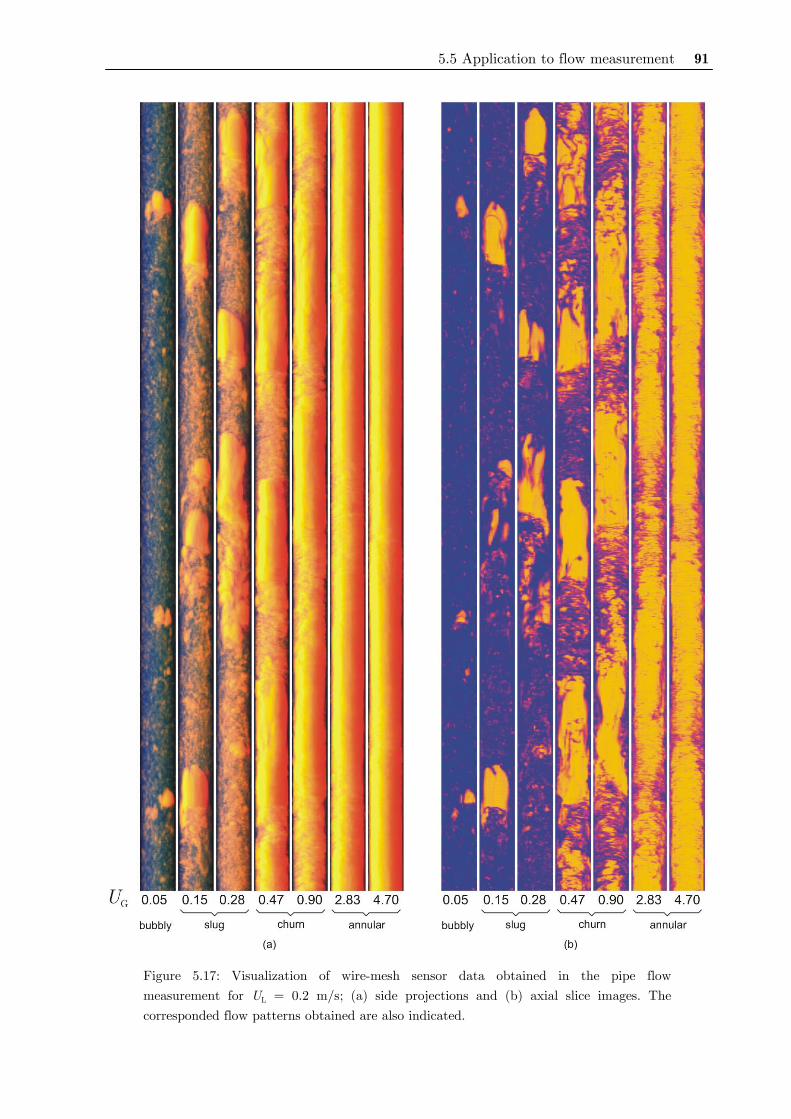
5.5 Application to flow measurement 91
Figure 5.17: Visualization of wire-mesh sensor data obtained in the pipe flow measurement for UL = 0.2 m/s; (a) side projections and (b) axial slice images. The corresponded flow patterns obtained are also indicated.
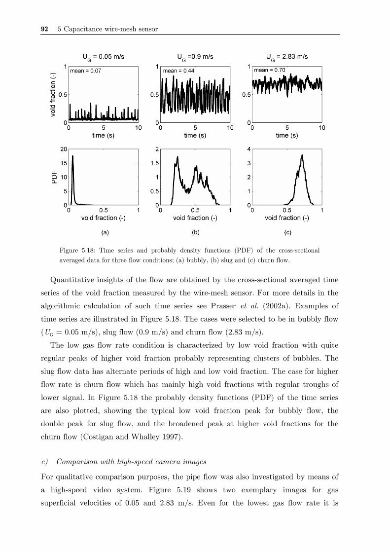
92 5 Capacitance wire-mesh sensor
Figure 5.18: Time series and probably density functions (PDF) of the cross-sectional averaged data for three flow conditions; (a) bubbly, (b) slug and (c) churn flow.
Quantitative insights of the flow are obtained by the cross-sectional averaged time
series of the void fraction measured by the wire-mesh sensor. For more details in the
algorithmic calculation of such time series see Prasser et al. (2002a). Examples of
time series are illustrated in Figure 5.18. The cases were selected to be in bubbly flow
(UG = 0.05 m/s), slug flow (0.9 m/s) and churn flow (2.83 m/s).
The low gas flow rate condition is characterized by low void fraction with quite
regular peaks of higher void fraction probably representing clusters of bubbles. The
slug flow data has alternate periods of high and low void fraction. The case for higher
flow rate is churn flow which has mainly high void fractions with regular troughs of
lower signal. In Figure 5.18 the probably density functions (PDF) of the time series
are also plotted, showing the typical low void fraction peak for bubbly flow, the
double peak for slug flow, and the broadened peak at higher void fractions for the
churn flow (Costigan and Whalley 1997).
c) Comparison with high-speed camera images
For qualitative comparison purposes, the pipe flow was also investigated by means of
a high-speed video system. Figure 5.19 shows two exemplary images for gas
superficial velocities of 0.05 and 2.83 m/s. Even for the lowest gas flow rate it is
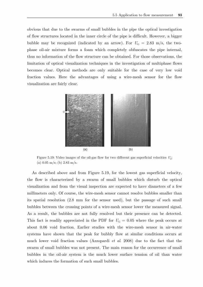
5.5 Application to flow measurement 93
obvious that due to the swarms of small bubbles in the pipe the optical investigation
of flow structures located in the inner circle of the pipe is difficult. However, a bigger
bubble may be recognized (indicated by an arrow). For UG = 2.83 m/s, the two-
phase oil-air mixture forms a foam which completely obfuscates the pipe internal,
thus no information of the flow structure can be obtained. For those observations, the
limitation of optical visualization techniques in the investigation of multiphase flows
becomes clear. Optical methods are only suitable for the case of very low void
fraction values. Here the advantages of using a wire-mesh sensor for the flow
visualization are fairly clear.
Figure 5.19: Video images of the oil-gas flow for two different gas superficial velocities Ug; (a) 0.05 m/s; (b) 2.83 m/s.
As described above and from Figure 5.19, for the lowest gas superficial velocity,
the flow is characterized by a swarm of small bubbles which disturb the optical
visualization and from the visual inspection are expected to have diameters of a few
millimeters only. Of course, the wire-mesh sensor cannot resolve bubbles smaller than
its spatial resolution (2.8 mm for the sensor used), but the passage of such small
bubbles between the crossing points of a wire-mesh sensor lower the measured signal.
As a result, the bubbles are not fully resolved but their presence can be detected.
This fact is readily appreciated in the PDF for UG = 0.05 where the peak occurs at
about 0.06 void fraction. Earlier studies with the wire-mesh sensor in air-water
systems have shown that the peak for bubbly flow at similar conditions occurs at
much lower void fraction values (Azzopardi et al. 2008) due to the fact that the
swarm of small bubbles was not present. The main reason for the occurrence of small
bubbles in the oil-air system is the much lower surface tension of oil than water
which induces the formation of such small bubbles.
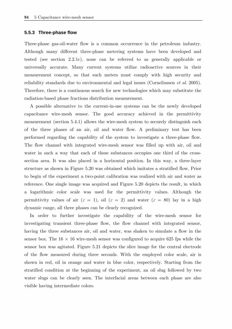
94 5 Capacitance wire-mesh sensor
5.5.3 Three-phase flow
Three-phase gas-oil-water flow is a common occurrence in the petroleum industry.
Although many different three-phase metering systems have been developed and
tested (see section 2.2.1c), none can be referred to as generally applicable or
universally accurate. Many current systems utilize radioactive sources in their
measurement concept, so that such meters must comply with high security and
reliability standards due to environmental and legal issues (Corneliussen et al. 2005).
Therefore, there is a continuous search for new technologies which may substitute the
radiation-based phase fractions distribution measurement.
A possible alternative to the current-in-use systems can be the newly developed
capacitance wire-mesh sensor. The good accuracy achieved in the permittivity
measurement (section 5.4.1) allows the wire-mesh system to securely distinguish each
of the three phases of an air, oil and water flow. A preliminary test has been
performed regarding the capability of the system to investigate a three-phase flow.
The flow channel with integrated wire-mesh sensor was filled up with air, oil and
water in such a way that each of these substances occupies one third of the cross-
section area. It was also placed in a horizontal position. In this way, a three-layer
structure as shown in Figure 5.20 was obtained which imitates a stratified flow. Prior
to begin of the experiment a two-point calibration was realized with air and water as
reference. One single image was acquired and Figure 5.20 depicts the result, in which
a logarithmic color scale was used for the permittivity values. Although the
permittivity values of air (ε = 1), oil (ε = 2) and water (ε = 80) lay in a high
dynamic range, all three phases can be clearly recognized.
In order to further investigate the capability of the wire-mesh sensor for
investigating transient three-phase flow, the flow channel with integrated sensor,
having the three substances air, oil and water, was shaken to simulate a flow in the
sensor box. The 16 × 16 wire-mesh sensor was configured to acquire 625 fps while the
sensor box was agitated. Figure 5.21 depicts the slice image for the central electrode
of the flow measured during three seconds. With the employed color scale, air is
shown in red, oil in orange and water in blue color, respectively. Starting from the
stratified condition at the beginning of the experiment, an oil slug followed by two
water slugs can be clearly seen. The interfacial areas between each phase are also
visible having intermediate colors.
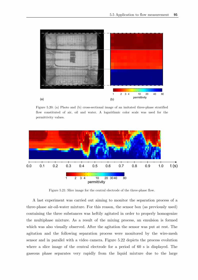
5.5 Application to flow measurement 95
Figure 5.20: (a) Photo and (b) cross-sectional image of an imitated three-phase stratified flow constituted of air, oil and water. A logarithmic color scale was used for the permittivity values.
Figure 5.21: Slice image for the central electrode of the three-phase flow.
A last experiment was carried out aiming to monitor the separation process of a
three-phase air-oil-water mixture. For this reason, the sensor box (as previously used)
containing the three substances was heftily agitated in order to properly homogenize
the multiphase mixture. As a result of the mixing process, an emulsion is formed
which was also visually observed. After the agitation the sensor was put at rest. The
agitation and the following separation process were monitored by the wire-mesh
sensor and in parallel with a video camera. Figure 5.22 depicts the process evolution
where a slice image of the central electrode for a period of 60 s is displayed. The
gaseous phase separates very rapidly from the liquid mixture due to the large
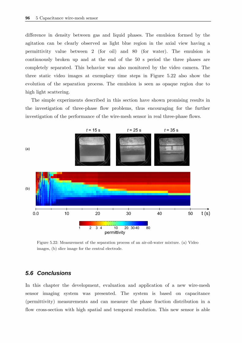
96 5 Capacitance wire-mesh sensor
difference in density between gas and liquid phases. The emulsion formed by the
agitation can be clearly observed as light blue region in the axial view having a
permittivity value between 2 (for oil) and 80 (for water). The emulsion is
continuously broken up and at the end of the 50 s period the three phases are
completely separated. This behavior was also monitored by the video camera. The
three static video images at exemplary time steps in Figure 5.22 also show the
evolution of the separation process. The emulsion is seen as opaque region due to
high light scattering.
The simple experiments described in this section have shown promising results in
the investigation of three-phase flow problems, thus encouraging for the further
investigation of the performance of the wire-mesh sensor in real three-phase flows.
Figure 5.22: Measurement of the separation process of an air-oil-water mixture. (a) Video images, (b) slice image for the central electrode.
5.6 Conclusions
In this chapter the development, evaluation and application of a new wire-mesh
sensor imaging system was presented. The system is based on capacitance
(permittivity) measurements and can measure the phase fraction distribution in a
flow cross-section with high spatial and temporal resolution. This new sensor is able
5.6 Conclusions 97
to measure in either electrically non-conducting or conducting fluids. The
investigation of the conductivity influence on the capacitive measuring circuit shows
that the wire-mesh sensor may be also applied to investigate conductive fluids with
conductivity values σ up to 1 S/m. In addition to the improved range of measurable
substances, another special advantage of the capacitance wire-mesh sensor is the
possibility to use electrically isolated wires, which enables to operate the sensor with
protective wire coatings, for instance in aggressive media.
The spatial sensitivity of a crossing point in the wire-mesh sensor for different
geometries has been analyzed by means of simulations with a commercial FEM
software. The results support the hitherto accepted assumption that the measurement
volume of a crossing point can be approximated by a cube centered at the crossing
point. Nevertheless, the exact sensitivity may be taken into account leading to an
improved measurement accuracy of a wire-mesh sensor.
The experimental evaluation of the prototype wire-mesh sensor system has shown
good reproducibility and accuracy in capacitance measurements even at a rather
short response time, thus allowing the system to be employed in the investigation of
a wide range of substances even with close permittivity values, such as for air and oil.
The good system accuracy also allows for the investigation of three-phase air-oil-
water mixtures. In preliminary experiments, the three phases in a stratified condition
as well as in a simulated flow were correctly acquired, and the emulsion formation
was also properly captured by the sensor. The evaluation of performance and
limitations of the sensor for three-phase flow applications must still be deepener
investigated in the future.

98 5 Capacitance wire-mesh sensor
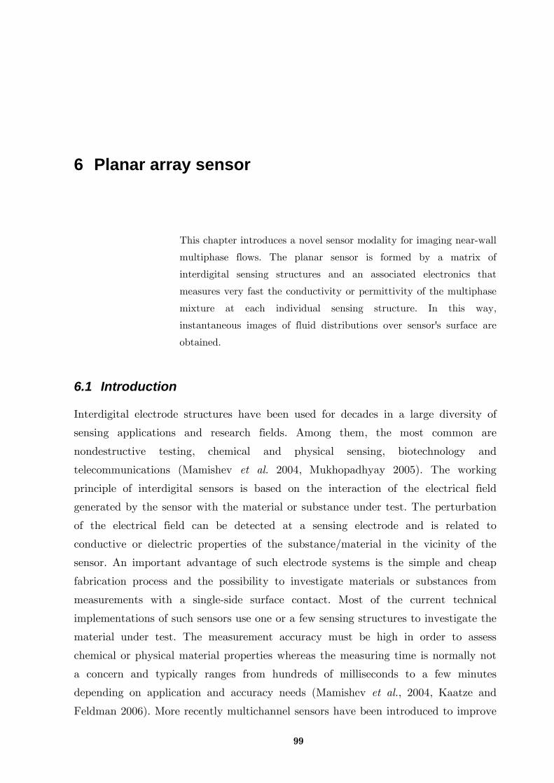
99
6 Planar array sensor
This chapter introduces a novel sensor modality for imaging near-wall
multiphase flows. The planar sensor is formed by a matrix of
interdigital sensing structures and an associated electronics that
measures very fast the conductivity or permittivity of the multiphase
mixture at each individual sensing structure. In this way,
instantaneous images of fluid distributions over sensor's surface are
obtained.
6.1 Introduction
Interdigital electrode structures have been used for decades in a large diversity of
sensing applications and research fields. Among them, the most common are
nondestructive testing, chemical and physical sensing, biotechnology and
telecommunications (Mamishev et al. 2004, Mukhopadhyay 2005). The working
principle of interdigital sensors is based on the interaction of the electrical field
generated by the sensor with the material or substance under test. The perturbation
of the electrical field can be detected at a sensing electrode and is related to
conductive or dielectric properties of the substance/material in the vicinity of the
sensor. An important advantage of such electrode systems is the simple and cheap
fabrication process and the possibility to investigate materials or substances from
measurements with a single-side surface contact. Most of the current technical
implementations of such sensors use one or a few sensing structures to investigate the
material under test. The measurement accuracy must be high in order to assess
chemical or physical material properties whereas the measuring time is normally not
a concern and typically ranges from hundreds of milliseconds to a few minutes
depending on application and accuracy needs (Mamishev et al., 2004, Kaatze and
Feldman 2006). More recently multichannel sensors have been introduced to improve
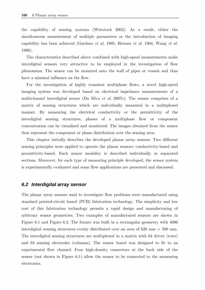
100 6 Planar array sensor
the capability of sensing systems (Wittstock 2002). As a result, either the
simultaneous measurement of multiple parameters or the introduction of imaging
capability has been achieved (Gardner et al. 1995, Hermes et al. 1994, Wang et al.
1996).
The characteristics described above combined with high-speed measurements make
interdigital sensors very attractive to be employed in the investigation of flow
phenomena. The sensor can be mounted onto the wall of pipes or vessels and thus
have a minimal influence on the flow.
For the investigation of highly transient multiphase flows, a novel high-speed
imaging system was developed based on electrical impedance measurements of a
multichannel interdigital sensor (Da Silva et al. 2007c). The sensor comprises of a
matrix of sensing structures which are individually measured in a multiplexed
manner. By measuring the electrical conductivity or the permittivity of the
interdigital sensing structures, phases of a multiphase flow or component
concentration can be visualized and monitored. The images obtained from the sensor
thus represent the component or phase distribution over the sensing area.
This chapter initially describes the developed planar array sensors. Two different
sensing principles were applied to operate the planar sensors: conductivity-based and
permittivity-based. Each sensor modality is described individually in separated
sections. Moreover, for each type of measuring principle developed, the sensor system
is experimentally evaluated and some flow applications are presented and discussed.
6.2 Interdigital array sensor
The planar array sensors used to investigate flow problems were manufactured using
standard printed-circuit board (PCB) fabrication technology. The simplicity and low
cost of this fabrication technology permits a rapid design and manufacturing of
arbitrary sensor geometries. Two examples of manufactured sensors are shown in
Figure 6.1 and Figure 6.2. The former was built in a rectangular geometry with 4096
interdigital sensing structures evenly distributed over an area of 620 mm × 500 mm.
The interdigital sensing structures are multiplexed in a matrix with 64 driver (rows)
and 64 sensing electrodes (columns). The sensor board was designed to fit to an
experimental flow channel. Four high-density connectors at the back side of the
sensor (not shown in Figure 6.1) allow the sensor to be connected to the measuring
electronics.
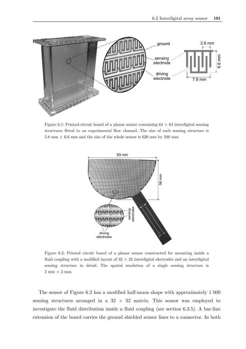
6.2 Interdigital array sensor 101
Figure 6.1: Printed-circuit board of a planar sensor containing 64 × 64 interdigital sensing structures fitted to an experimental flow channel. The size of each sensing structure is 5.8 mm × 6.6 mm and the size of the whole sensor is 620 mm by 500 mm.
Figure 6.2: Printed circuit board of a planar sensor constructed for mounting inside a fluid coupling with a modified layout of 32 × 32 interdigital electrodes and an interdigital sensing structure in detail. The spatial resolution of a single sensing structure is 2 mm × 3 mm.
The sensor of Figure 6.2 has a modified half-moon shape with approximately 1 000
sensing structures arranged in a 32 × 32 matrix. This sensor was employed to
investigate the fluid distribution inside a fluid coupling (see section 6.3.5). A bar-line
extension of the board carries the ground shielded sensor lines to a connector. In both

102 6 Planar array sensor
cases the electrodes are gold plated to reduce electrochemical effects during electrical
measurement.
6.3 Conductivity-based planar sensor
6.3.1 System description
The measuring electronics applied for the conductivity measurement is similar to the
electronics of a conductivity wire-mesh sensor (Prasser et al. 1998) and is described
below. Figure 6.3 depicts the block diagram of the measuring electronics for an
exemplary 64 × 64 electrodes configuration as well as the timing diagram for the
excitation-measuring scheme.
The transmitter electrodes are connected to a bipolar voltage source in a successive
order while all the other transmitter electrodes are connected to ground potential by
means of a set of analog switches. The outputs of the switches are buffered by
operational amplifiers in order to create a low impedance path. This step assures that
the potential of all transmitter electrodes, except the one of the currently activated
electrode, are at ground potential. A bipolar excitation voltage (dc-free) is employed
to avoid electrolysis effects.
The electrical currents flowing from the activated electrode to the sensing electrode
are converted to voltage by a set of auto-balancing bridge circuits. Since the quantity
of interest here is the electrical conductivity of the fluid over a sensing structure, the
auto-balancing bridge circuit is dimensioned to be resistance-dominant. The
capacitors in the feedback network of the opamps showed in Figure 6.3 serve only for
frequency compensation. Typical wave forms for the excitation and the measured
voltages are also shown in Figure 6.3. All voltages are analog-to-digital converted
simultaneously at the rising edge of the sample-and-hold signal. This routine is
repeated for all transmitter electrodes being activated. Once all transmitter electrodes
have been activated and all currents have been measured, one frame is obtained
containing 4096 values (for this sensor type) which corresponds to the distribution of
the electrical conductivity over the sensor surface.
The various frames acquired during a measurement are saved in an Nx × Ny × Nt
data matrix in computer memory, where Nx, Ny are the number of transmitter and
receiver electrodes and Nt denotes the number of time steps. The electronics is able to
produce up to 2 500 images per second.
6.3 Conductivity-based planar sensor 103
Figure 6.3: (a) Simplified block diagram of the measuring electronics. (b) Timing diagram for the multiplexed excitation and measuring scheme for the sensor. Voltages are sampled at the rising edge of the sample-and-hold signal. One frame is complete when the 64 transmitter electrodes have been activated and all currents have been measured. The signal SP denotes the polarity switch and S1 to S64 the analog switches.
6.3.2 Data processing
The voltage values measured by the surface sensor are proportional to the electrical
current flowing from the transmitter electrode to the receiver electrode. This current
basically depends on two parameters:
• the electrical conductivity σ of the liquid and
• the liquid wetting level (or liquid film thickness) of a sensing structure.
Depending on the application one of those two parameters can be explored to
generate information about the fluid distribution across the sensor. Since the system
generates only one measurement for two unknowns, one of the parameters must be
known beforehand or kept constant during the experiments to generate an
unambiguous output. In this way, two different situations can be investigated. In the
case the wetting level is constant, that means, the sensing structures are always
covered by a liquid, conductivity tracers can be applied to evaluate the flow in the
104 6 Planar array sensor
channel. The other choice is to measure the liquid distribution across the sensor
assuming the conductivity being constant. For instance, the presence of gas bubbles
on the surface can be detected due to the fact that the bubbles will change the
wetting level of a sensing structure.
The acquired voltages for all sensing structures are saved in a data matrix, in the
form ( ), ,V i j k where i and j denote spatial coordinates and k the temporal point
index. In principle, the evaluation of the measured voltage matrix ( ), ,V i j k would be
sufficient to investigate the component or phase distribution across the sensor
surface. However, differences in the electrical response of the individual transmitter-
receiver pairs, due to tolerances of electronic component or sensor elements, cause a
variance in the measured signals which in turn produces artifacts in the resulting
images. To compensate this variance two strategies are used to correct sensor’s
outputs depending on the measurement type, which are described bellow.
In the case that absolute conductivity values are to be assessed, the formula
( ) ( ) ( ) ( ), , , , , ,i j k V i j k a i j b i jσ = ⋅ + (6.1)
may be used for calibration, since the measured voltage is directly proportional to the
electrical conductivity of the liquid at the sensing structure. The parameters a(i,j)
and b(i,j) are determined from measurements with substances of known conductivity.
For this reason, data are firstly acquired with a substance of low conductivity σL
covering the whole sensor, thus producing the reference data matrix L( , )V i j .
Normally average values over a certain time are used to reduce statistical signal
fluctuations. This procedure is then repeated with the entire sensor surface covered
with another substance having a higher conductivity value σH, which gives the second
data matrix H( , )V i j . In this fashion, applying (6.1) for both measurement situations,
it is possible to determine them from
H L
H L( , )( , ) ( , )
a i jV i j V i j
σ σ−=−
, (6.2)
H L L H
H L
( , ) ( , )( , )( , ) ( , )
V i j V i jb i jV i j V i j
σ σ⋅ − ⋅=−
. (6.3)
Assuming the second situation described above, where the wetting level or phase
distributions are to be determined instead of conductivity values, the parameter
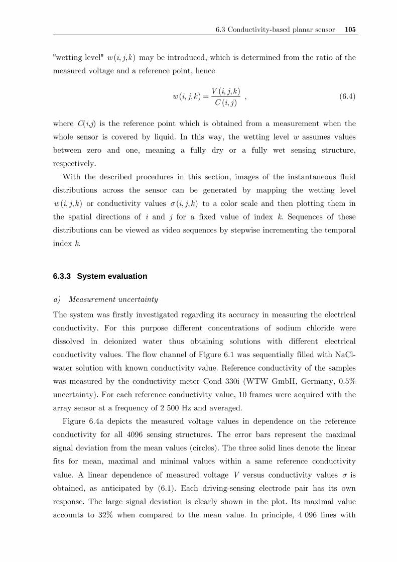
6.3 Conductivity-based planar sensor 105
"wetting level" ( ), ,w i j k may be introduced, which is determined from the ratio of the
measured voltage and a reference point, hence
( ) ( )( ), ,
, ,,
V i j kw i j k
C i j= , (6.4)
where C(i,j) is the reference point which is obtained from a measurement when the
whole sensor is covered by liquid. In this way, the wetting level w assumes values
between zero and one, meaning a fully dry or a fully wet sensing structure,
respectively.
With the described procedures in this section, images of the instantaneous fluid
distributions across the sensor can be generated by mapping the wetting level
( ), ,w i j k or conductivity values ( ), ,i j kσ to a color scale and then plotting them in
the spatial directions of i and j for a fixed value of index k. Sequences of these
distributions can be viewed as video sequences by stepwise incrementing the temporal
index k.
6.3.3 System evaluation
a) Measurement uncertainty
The system was firstly investigated regarding its accuracy in measuring the electrical
conductivity. For this purpose different concentrations of sodium chloride were
dissolved in deionized water thus obtaining solutions with different electrical
conductivity values. The flow channel of Figure 6.1 was sequentially filled with NaCl-
water solution with known conductivity value. Reference conductivity of the samples
was measured by the conductivity meter Cond 330i (WTW GmbH, Germany, 0.5%
uncertainty). For each reference conductivity value, 10 frames were acquired with the
array sensor at a frequency of 2 500 Hz and averaged.
Figure 6.4a depicts the measured voltage values in dependence on the reference
conductivity for all 4096 sensing structures. The error bars represent the maximal
signal deviation from the mean values (circles). The three solid lines denote the linear
fits for mean, maximal and minimal values within a same reference conductivity
value. A linear dependence of measured voltage V versus conductivity values σ is
obtained, as anticipated by (6.1). Each driving-sensing electrode pair has its own
response. The large signal deviation is clearly shown in the plot. Its maximal value
accounts to 32% when compared to the mean value. In principle, 4 096 lines with
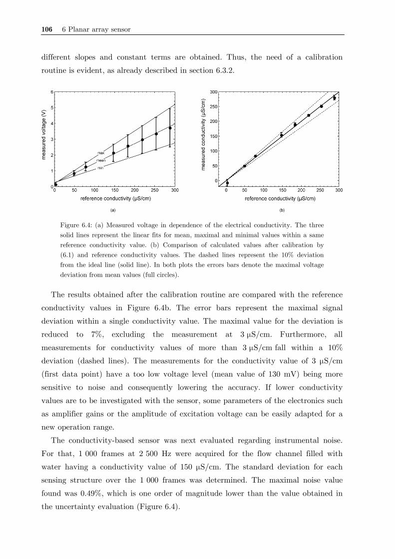
106 6 Planar array sensor
different slopes and constant terms are obtained. Thus, the need of a calibration
routine is evident, as already described in section 6.3.2.
Figure 6.4: (a) Measured voltage in dependence of the electrical conductivity. The three solid lines represent the linear fits for mean, maximal and minimal values within a same reference conductivity value. (b) Comparison of calculated values after calibration by (6.1) and reference conductivity values. The dashed lines represent the 10% deviation from the ideal line (solid line). In both plots the errors bars denote the maximal voltage deviation from mean values (full circles).
The results obtained after the calibration routine are compared with the reference
conductivity values in Figure 6.4b. The error bars represent the maximal signal
deviation within a single conductivity value. The maximal value for the deviation is
reduced to 7%, excluding the measurement at 3 μS/cm. Furthermore, all
measurements for conductivity values of more than 3 μS/cm fall within a 10%
deviation (dashed lines). The measurements for the conductivity value of 3 μS/cm
(first data point) have a too low voltage level (mean value of 130 mV) being more
sensitive to noise and consequently lowering the accuracy. If lower conductivity
values are to be investigated with the sensor, some parameters of the electronics such
as amplifier gains or the amplitude of excitation voltage can be easily adapted for a
new operation range.
The conductivity-based sensor was next evaluated regarding instrumental noise.
For that, 1 000 frames at 2 500 Hz were acquired for the flow channel filled with
water having a conductivity value of 150 μS/cm. The standard deviation for each
sensing structure over the 1 000 frames was determined. The maximal noise value
found was 0.49%, which is one order of magnitude lower than the value obtained in
the uncertainty evaluation (Figure 6.4).
6.3 Conductivity-based planar sensor 107
b) Depth sensitivity
In order to experimentally evaluate the depth sensitivity of the sensor, the following
experiment was carried out. The flow channel of Figure 6.1 with the integrated
planar sensor was firstly put in the horizontal position. An electrically non-
conducting glass plate of 120 mm × 200 mm size and 3 mm thickness was placed
over the planar sensor so that one of its endpoints was raised by a thin plastic spacer
of 1.5 mm thickness while the other one was in direct contact with the sensor,
forming an inclined plane as shown in Figure 6.5a. The flow channel was then filled
up with water (conductivity 250 μS/cm). In this way, a continuously growing water
thickness over the sensor in an area of 15 × 25 sensing structures was generated. In
the following analysis only this area was taken into account. Ten frames at 2 500 fps
were acquired and averaged. From the measured voltage values, the wetting levels
were computed from (6.4) and a calibration measurement which was previously taken
when the whole sensor was fully covered by water without plate. Figure 6.5b shows
the mean values over the 15 rows for the calculated wetting levels. The form of the
curve is an exponential rise which commensurate with previous analysis of interdigital
structures (Li et al. 2006).
Figure 6.5: (a) Experimental setup for the depth sensitivity estimation. (b) Wetting level response for different water thickness over the sensor surface.
There is no strict definition of penetration depth. Therefore the penetration depth
97γ of the sensor was defined as the liquid thickness producing a signal level which
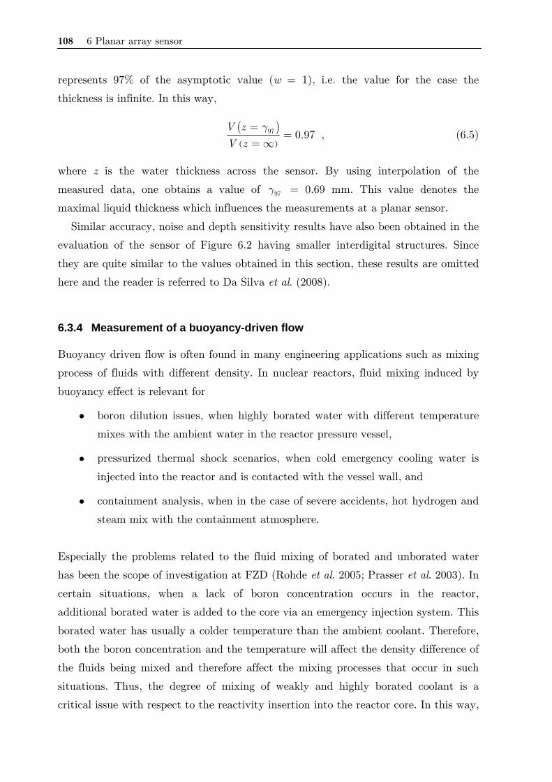
108 6 Planar array sensor
represents 97% of the asymptotic value (w = 1), i.e. the value for the case the
thickness is infinite. In this way,
( )( )
97 0.97V zV z
γ==
= ∞ , (6.5)
where z is the water thickness across the sensor. By using interpolation of the
measured data, one obtains a value of 97γ = 0.69 mm. This value denotes the
maximal liquid thickness which influences the measurements at a planar sensor.
Similar accuracy, noise and depth sensitivity results have also been obtained in the
evaluation of the sensor of Figure 6.2 having smaller interdigital structures. Since
they are quite similar to the values obtained in this section, these results are omitted
here and the reader is referred to Da Silva et al. (2008).
6.3.4 Measurement of a buoyancy-driven flow
Buoyancy driven flow is often found in many engineering applications such as mixing
process of fluids with different density. In nuclear reactors, fluid mixing induced by
buoyancy effect is relevant for
• boron dilution issues, when highly borated water with different temperature
mixes with the ambient water in the reactor pressure vessel,
• pressurized thermal shock scenarios, when cold emergency cooling water is
injected into the reactor and is contacted with the vessel wall, and
• containment analysis, when in the case of severe accidents, hot hydrogen and
steam mix with the containment atmosphere.
Especially the problems related to the fluid mixing of borated and unborated water
has been the scope of investigation at FZD (Rohde et al. 2005; Prasser et al. 2003). In
certain situations, when a lack of boron concentration occurs in the reactor,
additional borated water is added to the core via an emergency injection system. This
borated water has usually a colder temperature than the ambient coolant. Therefore,
both the boron concentration and the temperature will affect the density difference of
the fluids being mixed and therefore affect the mixing processes that occur in such
situations. Thus, the degree of mixing of weakly and highly borated coolant is a
critical issue with respect to the reactivity insertion into the reactor core. In this way,

6.3 Conductivity-based planar sensor 109
understanding the impact of such phenomena can help in the design and operation of
nuclear reactors.
The aim of the present study was to analyze the mixing processes related to the
boron dilution problem for safety-relevant scenarios in reactors. A simple vertical test
facility was constructed as nuclear reactor geometries are complex leading to the
mixing processes that are not widely understood or where the influence of the
buoyancy may not be significant.
a) Experimental setup
A vertical mixing test facility with simple geometry having rectangular cross section
was designed and constructed (Figure 6.6). Five identical rectangular segments as
described in Figure 6.1 are stacked together. Each segment is made of acrylic glass
which is 500 mm wide by 625 mm high by 100 mm deep. The whole test section is
3.32 m high. A flow inlet is located in between segments 1 and 2, while an outlet is
positioned in between segments 4 and 5. Segment number 2, right after the inlet, is
instrumented with the planar sensor. In this region the most interesting mixing
process occurs. The facility ensures that the gravity force acts along a significant
length scale.
In order to visualize the mixing process of two liquids having different densities in
a controlled manner, the following experiment was carried out. Water-glucose
mixtures were used to produce density gradients. A glucose-water solution containing
6% glucose has a corresponding density of 1020 kg⋅m-3, i.e. 2% density difference to
clean water. This is equivalent to about 60 K temperature difference. Furthermore,
sodium chloride was added to the higher density water-glucose solution acting as
tracer. In this way, the mixing process of clean water with the glucose-water solution
can be monitored by means of the planar sensor. It has been shown that the
conductivity measurement can be linked to the temperature or density gradients by
(Prasser et al. 2003)
( ) ( ) ( ) ( )L L L
H L H L H L
, , , , , ,, ,
i j k T i j k T i j ki j k
T Tσ σ ρ ρθ
σ σ ρ ρ− − −= ≅ ≅
− − −, (6.6)
where θ is called mixing scalar (assuming values between 0 and 1), σ is the measured
conductivity, T temperature and ρ density. The subscripts H and L stand for the
high and low values, respectively, which represent the parameter difference of the
used liquids. In the experiment described below, clean water and water-glucose
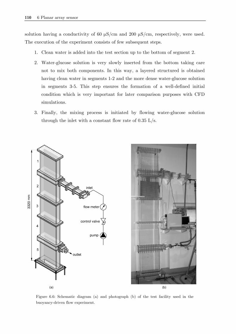
110 6 Planar array sensor
solution having a conductivity of 60 μS/cm and 200 μS/cm, respectively, were used.
The execution of the experiment consists of few subsequent steps.
1. Clean water is added into the test section up to the bottom of segment 2.
2. Water-glucose solution is very slowly inserted from the bottom taking care
not to mix both components. In this way, a layered structured is obtained
having clean water in segments 1-2 and the more dense water-glucose solution
in segments 3-5. This step ensures the formation of a well-defined initial
condition which is very important for later comparison purposes with CFD
simulations.
3. Finally, the mixing process is initiated by flowing water-glucose solution
through the inlet with a constant flow rate of 0.35 L/s.
Figure 6.6: Schematic diagram (a) and photograph (b) of the test facility used in the buoyancy-driven flow experiment.

6.3 Conductivity-based planar sensor 111
Figure 6.7: Instantaneous images of the mixing scalar θ. For details about the experiment see text.
b) Results
The mixing process was monitored with the planar sensor for 200 s at 300 fps. Since
the process is rather slow the frame frequency could also be lowered. Figure 6.7
depicts 12 instantaneous mixing scalar θ distributions over the sensor surface. In the
image for t = 0, the boundary between the two components and a transition region
can be observed. As the water-glucose solution flows into the channel, the formation
of a circular jet can be clearly seen. The subsequent images show the mixing of the
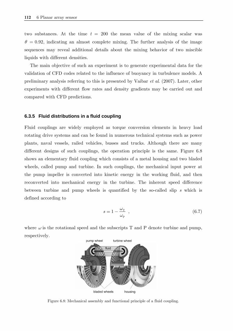
112 6 Planar array sensor
two substances. At the time t = 200 the mean value of the mixing scalar was
θ = 0.92, indicating an almost complete mixing. The further analysis of the image
sequences may reveal additional details about the mixing behavior of two miscible
liquids with different densities.
The main objective of such an experiment is to generate experimental data for the
validation of CFD codes related to the influence of buoyancy in turbulence models. A
preliminary analysis referring to this is presented by Vaibar et al. (2007). Later, other
experiments with different flow rates and density gradients may be carried out and
compared with CFD predictions.
6.3.5 Fluid distributions in a fluid coupling
Fluid couplings are widely employed as torque conversion elements in heavy load
rotating drive systems and can be found in numerous technical systems such as power
plants, naval vessels, railed vehicles, busses and trucks. Although there are many
different designs of such couplings, the operation principle is the same. Figure 6.8
shows an elementary fluid coupling which consists of a metal housing and two bladed
wheels, called pump and turbine. In such couplings, the mechanical input power at
the pump impeller is converted into kinetic energy in the working fluid, and then
reconverted into mechanical energy in the turbine. The inherent speed difference
between turbine and pump wheels is quantified by the so-called slip s which is
defined according to
T
P
1s ωω
= − , (6.7)
where ω is the rotational speed and the subscripts T and P denote turbine and pump,
respectively.
Figure 6.8: Mechanical assembly and functional principle of a fluid coupling.
6.3 Conductivity-based planar sensor 113
The power transmission characteristics of fluid couplings are highly influenced by
the fluid flow structure inside the coupling. The experimental investigation of the
flow characteristics inside a fluid coupling during operation is thus of great
importance for the optimization of static and transient behavior of those devices
(Höller 2000). However, so far it has been considered as impossible to perform
measurements on running fluid couplings due to their complex design as well as fast
rotational speed.
As an initial step towards the experimental investigation of fluid couplings, the
planar sensor technology was adapted to the measurement of two-phase flow patterns
in a blade channel of a fluid coupling during regular operation. In the following
sections, the experimental setup and some initial results are presented and discussed.
a) Experimental Setup
Experiments on a fluid coupling were carried out in the coupling test field of Voith
Turbo in Crailsheim, Germany. The coupling used in the experiments is a special test
coupling with a profile diameter of 422 mm which operates with water and has some
deviations from a standard design. Both shafts of the coupling extend to one side,
which is achieved by a hollow pump shaft enclosing the axial turbine shaft. This gives
full access to the coupling from one side and, thus, facilitated the mounting of the
electronics on the pump wheel. Both shafts are driven independently by two speed-
controlled electric motors. In this way, the rotational speed of the pump and turbine
and thereby the slip rate can be adjusted.
Two half-moon sensors (Figure 6.2) were mounted on the pressure-side and the
suction-side walls of a blade channel inside a test coupling (Figure 6.9). Two sensors
are required in order to visualize the flow at the two blade walls, pressure side wall
(upon which liquid is pushed by the tangential force), and the suction side wall (from
which liquid escapes by the action of tangential forces). Since it was technologically
easier, the sensors were mounted into different blade channels. This has no impact on
the measurement results since, due to symmetry, the flow can be considered being
similar in different channels.
A modified version of the conductivity-based electronics discussed in section 6.3.1
was used for such measurements. A major revision of the planar sensor electronics
was required to meet the requirements imposed by the conditions of a running fluid
coupling. The electronics have to be small, compact, and also able to rotate with the
coupling wheel. To comply with those constraints, the electronics was conceived (i) to
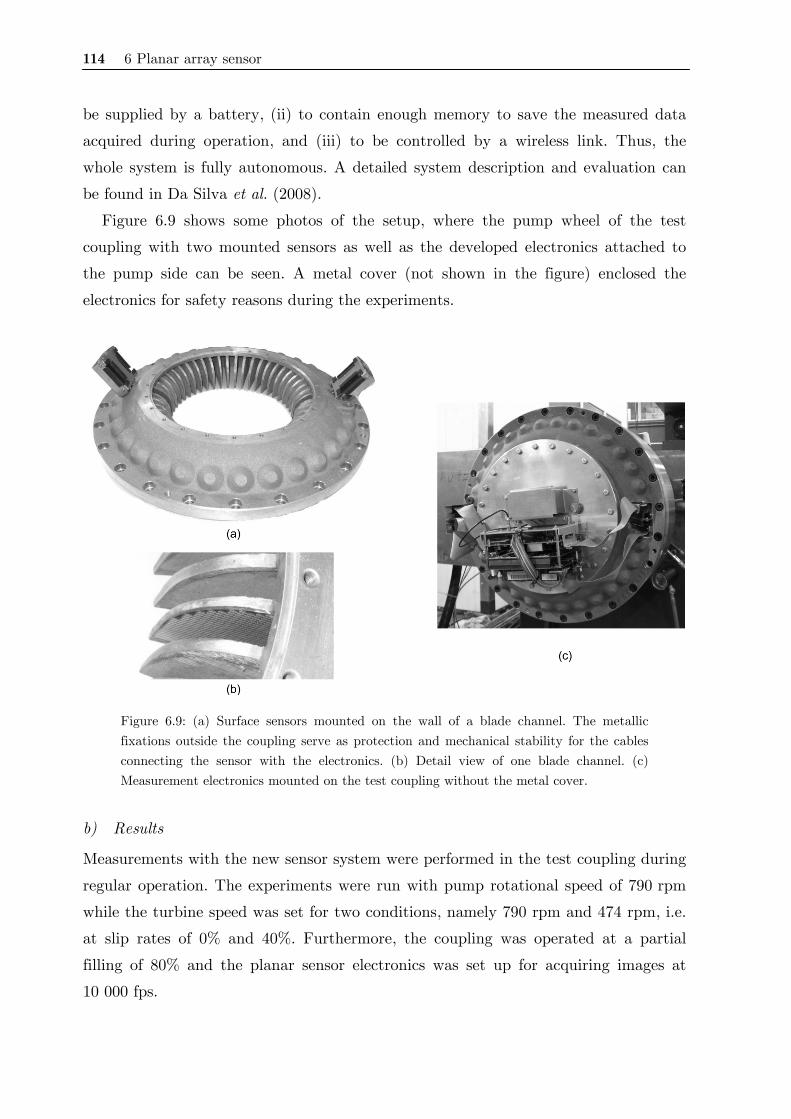
114 6 Planar array sensor
be supplied by a battery, (ii) to contain enough memory to save the measured data
acquired during operation, and (iii) to be controlled by a wireless link. Thus, the
whole system is fully autonomous. A detailed system description and evaluation can
be found in Da Silva et al. (2008).
Figure 6.9 shows some photos of the setup, where the pump wheel of the test
coupling with two mounted sensors as well as the developed electronics attached to
the pump side can be seen. A metal cover (not shown in the figure) enclosed the
electronics for safety reasons during the experiments.
Figure 6.9: (a) Surface sensors mounted on the wall of a blade channel. The metallic fixations outside the coupling serve as protection and mechanical stability for the cables connecting the sensor with the electronics. (b) Detail view of one blade channel. (c) Measurement electronics mounted on the test coupling without the metal cover.
b) Results
Measurements with the new sensor system were performed in the test coupling during
regular operation. The experiments were run with pump rotational speed of 790 rpm
while the turbine speed was set for two conditions, namely 790 rpm and 474 rpm, i.e.
at slip rates of 0% and 40%. Furthermore, the coupling was operated at a partial
filling of 80% and the planar sensor electronics was set up for acquiring images at
10 000 fps.
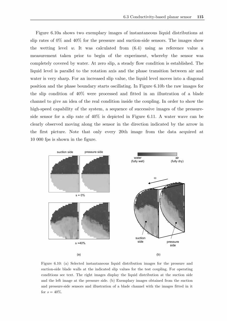
6.3 Conductivity-based planar sensor 115
Figure 6.10a shows two exemplary images of instantaneous liquid distributions at
slip rates of 0% and 40% for the pressure and suction-side sensors. The images show
the wetting level w. It was calculated from (6.4) using as reference value a
measurement taken prior to begin of the experiment, whereby the sensor was
completely covered by water. At zero slip, a steady flow condition is established. The
liquid level is parallel to the rotation axis and the phase transition between air and
water is very sharp. For an increased slip value, the liquid level moves into a diagonal
position and the phase boundary starts oscillating. In Figure 6.10b the raw images for
the slip condition of 40% were processed and fitted in an illustration of a blade
channel to give an idea of the real condition inside the coupling. In order to show the
high-speed capability of the system, a sequence of successive images of the pressure-
side sensor for a slip rate of 40% is depicted in Figure 6.11. A water wave can be
clearly observed moving along the sensor in the direction indicated by the arrow in
the first picture. Note that only every 20th image from the data acquired at
10 000 fps is shown in the figure.
Figure 6.10: (a) Selected instantaneous liquid distribution images for the pressure and suction-side blade walls at the indicated slip values for the test coupling. For operating conditions see text. The right images display the liquid distribution at the suction side and the left image at the pressure side. (b) Exemplary images obtained from the suction and pressure-side sensors and illustration of a blade channel with the images fitted in it for s = 40%.
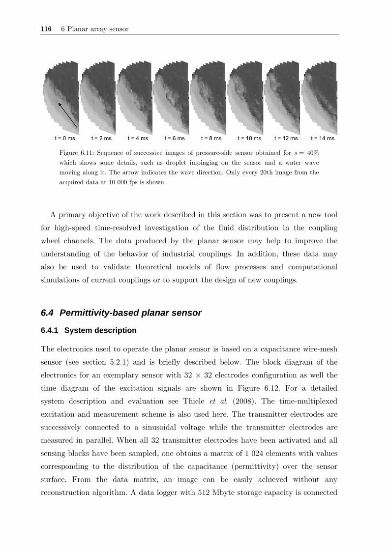
116 6 Planar array sensor
Figure 6.11: Sequence of successive images of pressure-side sensor obtained for s = 40% which shows some details, such as droplet impinging on the sensor and a water wave moving along it. The arrow indicates the wave direction. Only every 20th image from the acquired data at 10 000 fps is shown.
A primary objective of the work described in this section was to present a new tool
for high-speed time-resolved investigation of the fluid distribution in the coupling
wheel channels. The data produced by the planar sensor may help to improve the
understanding of the behavior of industrial couplings. In addition, these data may
also be used to validate theoretical models of flow processes and computational
simulations of current couplings or to support the design of new couplings.
6.4 Permittivity-based planar sensor
6.4.1 System description
The electronics used to operate the planar sensor is based on a capacitance wire-mesh
sensor (see section 5.2.1) and is briefly described below. The block diagram of the
electronics for an exemplary sensor with 32 × 32 electrodes configuration as well the
time diagram of the excitation signals are shown in Figure 6.12. For a detailed
system description and evaluation see Thiele et al. (2008). The time-multiplexed
excitation and measurement scheme is also used here. The transmitter electrodes are
successively connected to a sinusoidal voltage while the transmitter electrodes are
measured in parallel. When all 32 transmitter electrodes have been activated and all
sensing blocks have been sampled, one obtains a matrix of 1 024 elements with values
corresponding to the distribution of the capacitance (permittivity) over the sensor
surface. From the data matrix, an image can be easily achieved without any
reconstruction algorithm. A data logger with 512 Mbyte storage capacity is connected
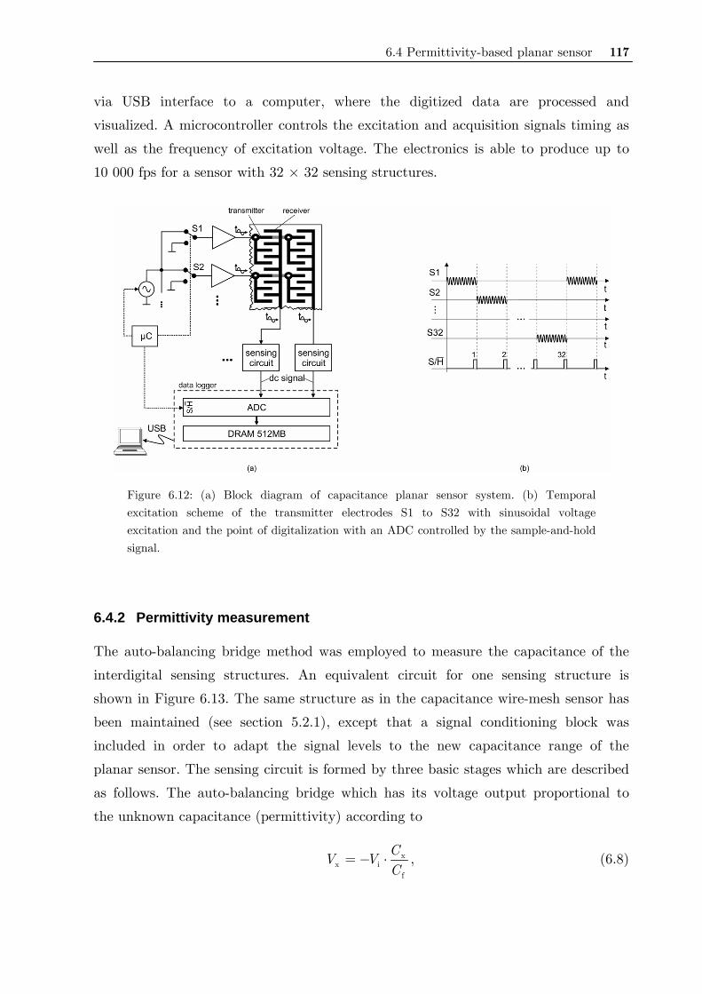
6.4 Permittivity-based planar sensor 117
via USB interface to a computer, where the digitized data are processed and
visualized. A microcontroller controls the excitation and acquisition signals timing as
well as the frequency of excitation voltage. The electronics is able to produce up to
10 000 fps for a sensor with 32 × 32 sensing structures.
Figure 6.12: (a) Block diagram of capacitance planar sensor system. (b) Temporal excitation scheme of the transmitter electrodes S1 to S32 with sinusoidal voltage excitation and the point of digitalization with an ADC controlled by the sample-and-hold signal.
6.4.2 Permittivity measurement
The auto-balancing bridge method was employed to measure the capacitance of the
interdigital sensing structures. An equivalent circuit for one sensing structure is
shown in Figure 6.13. The same structure as in the capacitance wire-mesh sensor has
been maintained (see section 5.2.1), except that a signal conditioning block was
included in order to adapt the signal levels to the new capacitance range of the
planar sensor. The sensing circuit is formed by three basic stages which are described
as follows. The auto-balancing bridge which has its voltage output proportional to
the unknown capacitance (permittivity) according to
xx i
f
CV VC
= − ⋅ , (6.8)
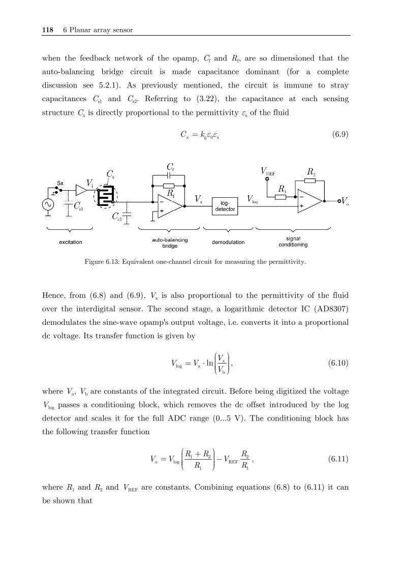
118 6 Planar array sensor
when the feedback network of the opamp, Cf and Rf, are so dimensioned that the
auto-balancing bridge circuit is made capacitance dominant (for a complete
discussion see 5.2.1). As previously mentioned, the circuit is immune to stray
capacitances Cs1 and Cs2. Referring to (3.22), the capacitance at each sensing
structure Cx is directly proportional to the permittivity εx of the fluid
x g 0 xC k ε ε= (6.9)
Figure 6.13: Equivalent one-channel circuit for measuring the permittivity.
Hence, from (6.8) and (6.9), Vx is also proportional to the permittivity of the fluid
over the interdigital sensor. The second stage, a logarithmic detector IC (AD8307)
demodulates the sine-wave opamp's output voltage, i.e. converts it into a proportional
dc voltage. Its transfer function is given by
xlog a
b
ln VV VV
⎛ ⎞⎟⎜ ⎟= ⋅ ⎜ ⎟⎜ ⎟⎜⎝ ⎠, (6.10)
where Va, Vb are constants of the integrated circuit. Before being digitized the voltage
Vlog passes a conditioning block, which removes the dc offset introduced by the log
detector and scales it for the full ADC range (0...5 V). The conditioning block has
the following transfer function
1 2 2o log REF
1 1
R R RV V VR R
⎛ ⎞+ ⎟⎜ ⎟= −⎜ ⎟⎜ ⎟⎜⎝ ⎠, (6.11)
where R1 and R2 and VREF are constants. Combining equations (6.8) to (6.11) it can
be shown that

6.4 Permittivity-based planar sensor 119
( )o xlnV a bε= ⋅ + , (6.12)
where a and b are constants that encompass all the circuit constants. Consequently,
the measured voltage Vo effectively represents the permittivity of the sensing
structures. The logarithmic response assures the measurement of even very small
permittivity values.
Due to small intrinsic differences of the employed ICs and tolerances in resistor
and capacitor values, there is a variance in the measured voltage over all
measurement channels. Thus, calibration of these channels is necessary to achieve
reliable output readings. A similar calibration routine as described in section 5.2.2
must be performed and is shortly described below.
For the calibration routine, first the surface sensor is fully covered with a
substance of low permittivity εL, in most cases air εL = 1, and the data matrix LoV is
acquired for all sensing structures i and j. Usually average values over a definite time
are used to reduce the influence of noise. A second data matrix HoV is acquired for
the situation the sensor is covered with a substance of high permittivity εH. In the
case that the lower permittivity reference substance is air with ε = 1, the calculation
of εx simplifies to (section 5.2.2)
( )L
o ox HH L
o o
( , , ) ( , )( , , ) exp ln( , ) ( , )
V i j k V i ji j kV i j V i j
ε ε⎛ ⎞− ⎟⎜ ⎟= ⎜ ⎟⎜ ⎟⎜ −⎝ ⎠
. (6.13)
6.4.3 System evaluation
a) Measurement uncertainty
A similar approach as described in section 6.3.3 for the evaluation of the
conductivity-based system was also applied. The sensor used for the experimental
evaluation is shown in Figure 6.14. The geometry of the interdigital structure is the
same as for the sensor of Figure 6.2, but a rectangular sensor geometry was used. An
acrylic box of 35 mm height is mounted around the sensing area serving as vessel for
the liquids to be investigated.
First, the system was evaluated regarding accuracy, where five different substances
and air (empty sensor) in a permittivity range from 1 to 80 were measured. The
reference permittivity values ε are listed in Table 6.1. For each substance, 10 frames
were acquired at 10 kHz and an average value was taken to reduce random noise.
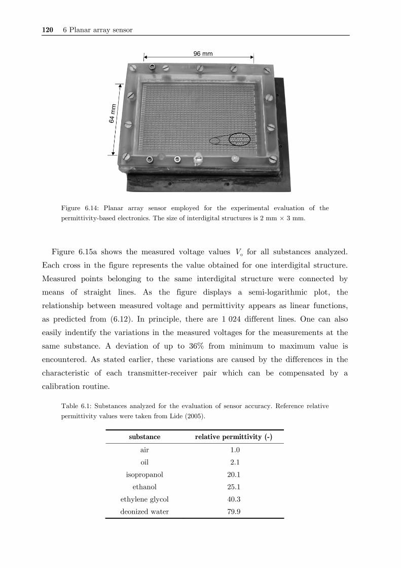
120 6 Planar array sensor
Figure 6.14: Planar array sensor employed for the experimental evaluation of the permittivity-based electronics. The size of interdigital structures is 2 mm × 3 mm.
Figure 6.15a shows the measured voltage values Vo for all substances analyzed.
Each cross in the figure represents the value obtained for one interdigital structure.
Measured points belonging to the same interdigital structure were connected by
means of straight lines. As the figure displays a semi-logarithmic plot, the
relationship between measured voltage and permittivity appears as linear functions,
as predicted from (6.12). In principle, there are 1 024 different lines. One can also
easily indentify the variations in the measured voltages for the measurements at the
same substance. A deviation of up to 36% from minimum to maximum value is
encountered. As stated earlier, these variations are caused by the differences in the
characteristic of each transmitter-receiver pair which can be compensated by a
calibration routine.
Table 6.1: Substances analyzed for the evaluation of sensor accuracy. Reference relative permittivity values were taken from Lide (2005).
substance relative permittivity (-)
air 1.0
oil 2.1
isopropanol 20.1
ethanol 25.1
ethylene glycol 40.3
deonized water 79.9
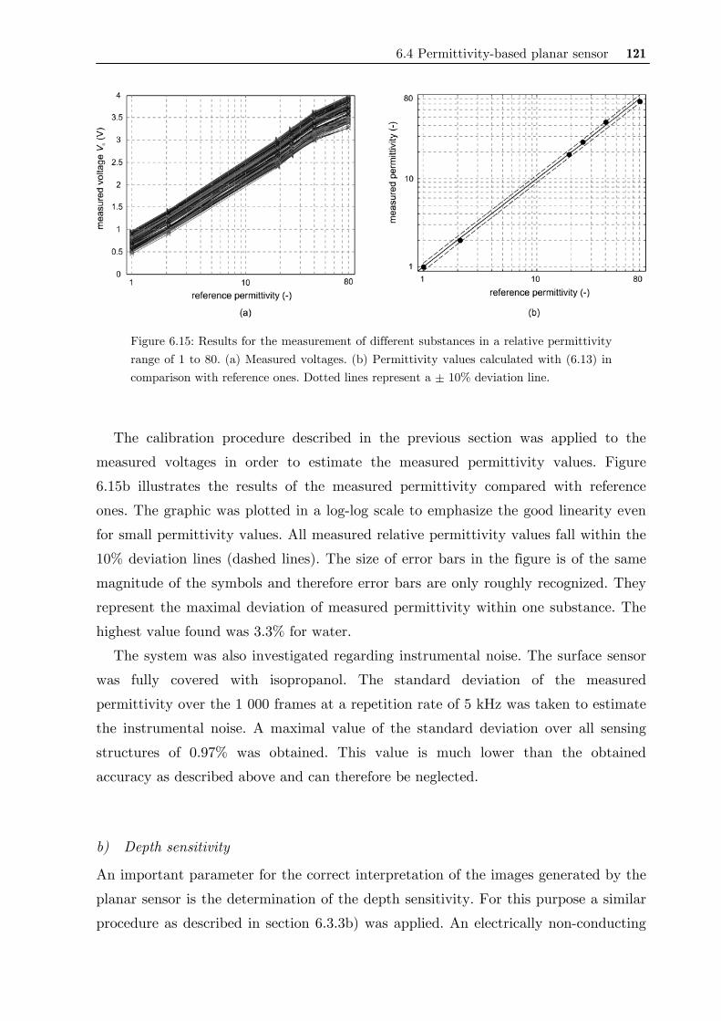
6.4 Permittivity-based planar sensor 121
Figure 6.15: Results for the measurement of different substances in a relative permittivity range of 1 to 80. (a) Measured voltages. (b) Permittivity values calculated with (6.13) in comparison with reference ones. Dotted lines represent a ± 10% deviation line.
The calibration procedure described in the previous section was applied to the
measured voltages in order to estimate the measured permittivity values. Figure
6.15b illustrates the results of the measured permittivity compared with reference
ones. The graphic was plotted in a log-log scale to emphasize the good linearity even
for small permittivity values. All measured relative permittivity values fall within the
10% deviation lines (dashed lines). The size of error bars in the figure is of the same
magnitude of the symbols and therefore error bars are only roughly recognized. They
represent the maximal deviation of measured permittivity within one substance. The
highest value found was 3.3% for water.
The system was also investigated regarding instrumental noise. The surface sensor
was fully covered with isopropanol. The standard deviation of the measured
permittivity over the 1 000 frames at a repetition rate of 5 kHz was taken to estimate
the instrumental noise. A maximal value of the standard deviation over all sensing
structures of 0.97% was obtained. This value is much lower than the obtained
accuracy as described above and can therefore be neglected.
b) Depth sensitivity
An important parameter for the correct interpretation of the images generated by the
planar sensor is the determination of the depth sensitivity. For this purpose a similar
procedure as described in section 6.3.3b) was applied. An electrically non-conducting
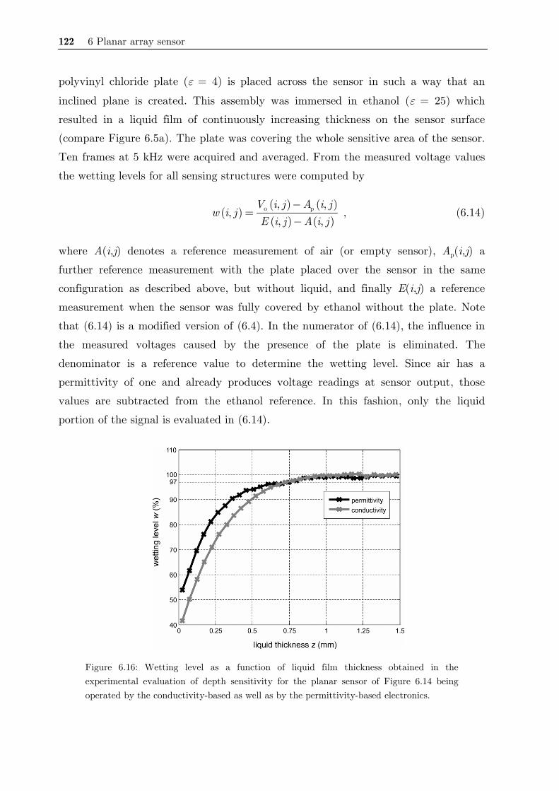
122 6 Planar array sensor
polyvinyl chloride plate (ε = 4) is placed across the sensor in such a way that an
inclined plane is created. This assembly was immersed in ethanol (ε = 25) which
resulted in a liquid film of continuously increasing thickness on the sensor surface
(compare Figure 6.5a). The plate was covering the whole sensitive area of the sensor.
Ten frames at 5 kHz were acquired and averaged. From the measured voltage values
the wetting levels for all sensing structures were computed by
( )( ) ( )( ) ( )
o p, ,,
, ,V i j A i j
w i jE i j A i j
−=
− , (6.14)
where A(i,j) denotes a reference measurement of air (or empty sensor), Ap(i,j) a
further reference measurement with the plate placed over the sensor in the same
configuration as described above, but without liquid, and finally E(i,j) a reference
measurement when the sensor was fully covered by ethanol without the plate. Note
that (6.14) is a modified version of (6.4). In the numerator of (6.14), the influence in
the measured voltages caused by the presence of the plate is eliminated. The
denominator is a reference value to determine the wetting level. Since air has a
permittivity of one and already produces voltage readings at sensor output, those
values are subtracted from the ethanol reference. In this fashion, only the liquid
portion of the signal is evaluated in (6.14).
Figure 6.16: Wetting level as a function of liquid film thickness obtained in the experimental evaluation of depth sensitivity for the planar sensor of Figure 6.14 being operated by the conductivity-based as well as by the permittivity-based electronics.
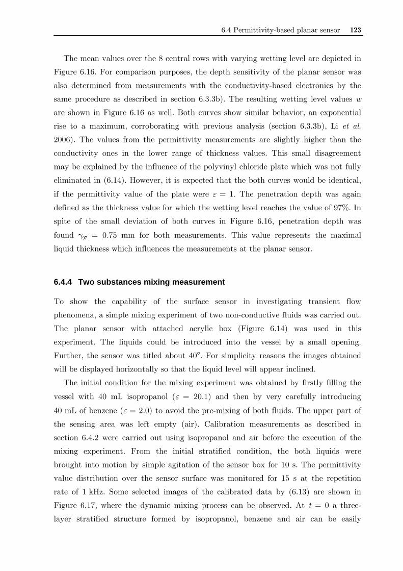
6.4 Permittivity-based planar sensor 123
The mean values over the 8 central rows with varying wetting level are depicted in
Figure 6.16. For comparison purposes, the depth sensitivity of the planar sensor was
also determined from measurements with the conductivity-based electronics by the
same procedure as described in section 6.3.3b). The resulting wetting level values w
are shown in Figure 6.16 as well. Both curves show similar behavior, an exponential
rise to a maximum, corroborating with previous analysis (section 6.3.3b), Li et al.
2006). The values from the permittivity measurements are slightly higher than the
conductivity ones in the lower range of thickness values. This small disagreement
may be explained by the influence of the polyvinyl chloride plate which was not fully
eliminated in (6.14). However, it is expected that the both curves would be identical,
if the permittivity value of the plate were ε = 1. The penetration depth was again
defined as the thickness value for which the wetting level reaches the value of 97%. In
spite of the small deviation of both curves in Figure 6.16, penetration depth was
found γ97 = 0.75 mm for both measurements. This value represents the maximal
liquid thickness which influences the measurements at the planar sensor.
6.4.4 Two substances mixing measurement
To show the capability of the surface sensor in investigating transient flow
phenomena, a simple mixing experiment of two non-conductive fluids was carried out.
The planar sensor with attached acrylic box (Figure 6.14) was used in this
experiment. The liquids could be introduced into the vessel by a small opening.
Further, the sensor was titled about 40°. For simplicity reasons the images obtained
will be displayed horizontally so that the liquid level will appear inclined.
The initial condition for the mixing experiment was obtained by firstly filling the
vessel with 40 mL isopropanol (ε = 20.1) and then by very carefully introducing
40 mL of benzene (ε = 2.0) to avoid the pre-mixing of both fluids. The upper part of
the sensing area was left empty (air). Calibration measurements as described in
section 6.4.2 were carried out using isopropanol and air before the execution of the
mixing experiment. From the initial stratified condition, the both liquids were
brought into motion by simple agitation of the sensor box for 10 s. The permittivity
value distribution over the sensor surface was monitored for 15 s at the repetition
rate of 1 kHz. Some selected images of the calibrated data by (6.13) are shown in
Figure 6.17, where the dynamic mixing process can be observed. At t = 0 a three-
layer stratified structure formed by isopropanol, benzene and air can be easily
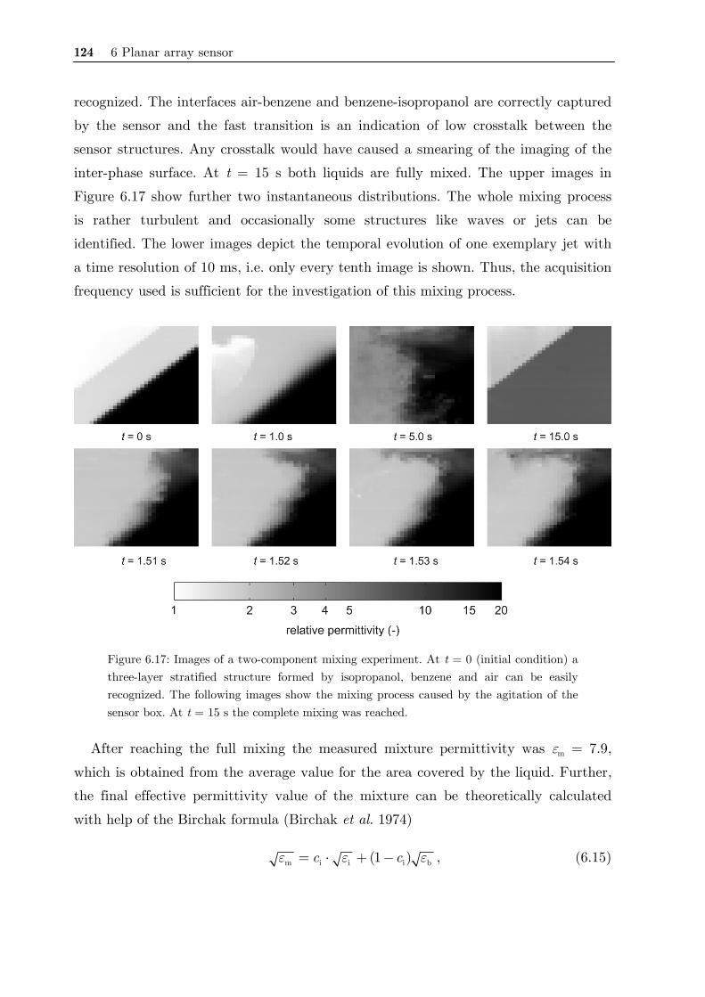
124 6 Planar array sensor
recognized. The interfaces air-benzene and benzene-isopropanol are correctly captured
by the sensor and the fast transition is an indication of low crosstalk between the
sensor structures. Any crosstalk would have caused a smearing of the imaging of the
inter-phase surface. At t = 15 s both liquids are fully mixed. The upper images in
Figure 6.17 show further two instantaneous distributions. The whole mixing process
is rather turbulent and occasionally some structures like waves or jets can be
identified. The lower images depict the temporal evolution of one exemplary jet with
a time resolution of 10 ms, i.e. only every tenth image is shown. Thus, the acquisition
frequency used is sufficient for the investigation of this mixing process.
Figure 6.17: Images of a two-component mixing experiment. At t = 0 (initial condition) a three-layer stratified structure formed by isopropanol, benzene and air can be easily recognized. The following images show the mixing process caused by the agitation of the sensor box. At t = 15 s the complete mixing was reached.
After reaching the full mixing the measured mixture permittivity was εm = 7.9,
which is obtained from the average value for the area covered by the liquid. Further,
the final effective permittivity value of the mixture can be theoretically calculated
with help of the Birchak formula (Birchak et al. 1974)
m i i i b(1 )c cε ε ε= ⋅ + − , (6.15)
6.5 Conclusions 125
where ci is the isopropanol concentration, εi and εb are the permittivities of
isopropanol and benzene, respectively. The isopropanol concentration is obtained
from the volume fractions of each liquid ci = 0.5 (= 40 mL/80 mL). Since εI = 20.1
and εb = 2.0, from (6.15) the mixture permittivity is calculated to be 8.69. The
measured value is very close to the theoretical value and the relative deviation of the
measured permittivity is 9.1%.
6.5 Conclusions
A new sensor modality for the investigation of fluid flow phenomena has been
developed and tested. The planar sensor comprises an array of interdigital sensors
which are individually interrogated in a multiplexed manner at very fast repetition
rate. The coplanar electrodes configuration allows the sensor to be placed on the wall
of pipes or vessels and thus having a minimal influence on the flow.
The new sensor can be operated either with a conductivity-based electronics or a
permittivity-based one. The planar sensor is able to detect phases or components in
dynamic fluid flow. The electronics performs a two-dimensional measurement of an
electrical parameter (conductivity or permittivity) of interdigital sensing structures,
which effectively gives images of the instantaneous fluid distribution over the sensor
surface.
Both systems are able to perform measurements at up to 10 000 fps which allows
the investigation of highly transient flows. Both electronics present good accuracy
and low noise even at rather high measuring frequencies. The depth sensitivity has
been also experimentally determined showing results compatible with other studies.
Besides the sensor characterization, a few flow measurement experiments were
presented and discussed, thus indicating some application fields for the novel sensors.
Further work may encompass optimization of the interdigital electrode structure
with help of electric field simulations to improve depth sensitivity or signal quality.
Furthermore, the use of the presented sensors in similar flow problems is planned
serving as basis for better understanding of such flows or as validation data base for
CFD codes.

126 6 Planar array sensor
127
7 Conclusions
In this concluding chapter the main achievements of the thesis are
summarized as well as some issues for future work are discussed.
7.1 Conclusions
The experimental investigation of multiphase flow is essential to the better
understanding and optimization of processes and devices in many engineering
applications. The measurement of multiphase flow also forms the basis for validation
of models and simulations. In this work, impedance sensors for the measurement and
imaging of gas-liquid multiphase flows were investigated and tested. Specifically three
different sensor systems were developed, characterized with indications to
measurement uncertainty, advantages and limitations, as well as applied in some
potential applications.
The complex permittivity needle probe (Chapter 4) may be used for local
multiphase flow measurement. It measures simultaneously and very fast the
conductivity and permittivity values of fluids at the probe tip. It has been applied to
measure oil-gas-water three-phase flow and also to monitor the mixing of two
substances in a chemical reactor.
Cross-sectional images of a pipe flow can be obtained be means of the newly
developed capacitance wire-mesh sensor (Chapter 5). It is a further development of
current conductivity sensors. The range of substances, it may be applied to, is now
not limited to conducting liquids. Maximal frame rates of 10 kfps have been reached,
which places this sensor among the fastest imaging techniques. High spatial and
temporal resolution images of gas-oil two-phase flow have been obtained.
Furthermore, the sensor may also be applied for the investigation of three-phase
flows, whereby initial measurements have shown promising results.
128 7 Conclusions
A new sensor modality was also presented within the work of this thesis. A planar
array sensor was proposed to investigate fluid distributions along the surface of
objects and near-wall flows (Chapter 6). It can be operated by a conductivity-based
as well as permittivity-based electronics. In this way, a number of applications are
possible. This sensor was successfully applied to investigate the liquid distribution
inside a fluid coupling during regular operation rotating at 790 rpm, to the
visualization of mixing process of scenarios relevant to nuclear safety, and to the
visualization of mixing of two non-conducting liquids.
All sensor systems present high-speed capability thus being well suited for
investigation of transient phenomena. The applications presented within this work
are evidently not exhaustive, but serve as basis to the deployment of the developed
sensor systems for future work.
The main contribution of this research work to the field of multiphase flow
measurement technology is therefore the development, characterization and
application of new sensors based on electrical impedance measurement. All sensors
were optimized with respect to a very high measurement speed and two of them offer
the capability for two-dimensional measurement (phase fraction imaging). The
sensors are furthermore very robust and can easily be employed in a number of
applications in research and industry.
7.2 Outlook
As already stated, the main task for the future is to employ the newly developed
sensors for systematic investigation of flow phenomena or to search industrial
applications for them. Nevertheless, for future research, it is interesting to have a
closer look at following points.
• The needle probe may be provided with a miniature thermocouple thus
generating a three-modality probe. Further, the temperature information may
be used to compensate conductivity/permittivity readings.
• The exact spatial sensitivity distribution of a wire-mesh sensor, as described in
section 5.3.3, may be taken into account in the image processing algorithm
possibility leading to an improvement in the measurement accuracy.

7.2 Outlook 129
• The capability and limitations of the use of the capacitance wire-mesh sensor
for the investigation of three-phase flows should be carried on, as already
started in section 5.5.3.
• Other geometries for the sensing structures of planar sensors may be
investigated aiming to optimize signal sensitivity or penetration depth.
• The development of dual-modality electronics for wire-mesh and planar array
may be investigated which perform simultaneous conductivity and permittivity
measurements.

130 7 Conclusions
131
References
Adrian, R.J. 1991 Particle-imaging techniques for experimental fluid mechanics.
Annual Review of Fluid Mechanics 23 261–304.
Agilent 2006a Basics of Measuring the Dielectric Properties of Materials. Application
Note, Agilent Technologies, June 2006.Available at: <http://www.agilent.com>
Agilent 2006b The Impedance Measurement Handbook. Application Note, Agilent
Technologies, July 2006. Available at: <http://www.agilent.com>
Ahmed W.H. 2006 Capacitance sensors for void-fraction measurements and flow-
pattern identification in air–oil two-phase flow. IEEE Sensors Journal 6 1153-
1163.
Andreussi P., Di Donfrancesco A. and Messia M. 1988 An impedance method for the
measurement of liquid hold-up in two phase flow. International Journal of
Multiphase Flow 14 777–785.
Ansys, Inc. 2008 Ansys CFX [online]. [Accessed 10th March 2008]:
<http://www.ansys.com/Products/cfx.asp>.
Asali J.C., Hanratty T.J., and Andreussi P. 1985 Interfacial drag and film height for
vertical annular flow. AIChE Journal 31 895–902.
Azzopardi B. 2006 Gas-liquid Flows. New York: Begell House.
Azzopardi B.J., Hernandez Perez V., Kaji R., da Silva M.J., Beyer M., and Hampel
U. 2008 Wire mesh sensor studies in a vertical pipe. In: HEAT 2008, Fifth
International Conference on Transport Phenomena in Multiphase Systems, June
30 - July 3, Bialystok, Poland.
Babelli I.M.M. 2002 In search of an ideal multiphase flow meter for the oil industry.
The Arabian Journal for Science and Engineering 27 113-126.
Baker R.C. 2000 Flow Measurement Handbook: Industrial Designs, Operating
Principles, Performance, and Applications. Cambridge, UK: Cambridge
University Press.

132 References
Barnea D. 1987 A unified model for predicting flow-pattern transitions for the whole
range of pipe inclinations. International Journal of Multiphase Flow 13 1-12.
Bauckhage K. 1996 Gleichzeitige Erfassung von Partikelmerkmalen und
Eigenschaften mehrphasiger Strömungen mit Hilfe der Phasen-Doppler-
Anemometrie. Chemie Ingenieur Technik 68 253-266.
Bera S.C. and Chattopadhyay S. 2003 A modified Schering bridge for measurement
of the dielectric parameters of a material and the capacitance of a capacitive
transducer. Measurement 33 3–7.
Bertola V. 2003 Two-phase flow measurement techniques, p. 281-323. In: Modeling
and Experimentation in Two-Phase Flow, Bertola V. (ed) New York: Springer.
Bieberle M., Fischer F., Schleicher E., Hampel U., Koch D., Aktay K.S.C., Menz H.-
J., and Mayer H.-G. 2007 Ultrafast limited-angle-type x-ray tomography.
Applied Physics Letters 91 123516.
Birchak J.R., Gardner C.G., Hipp J.E., and Victor J.M. 1974 High dielectric-constant
microwave probes for sensing soil-moisture. Proceedings of the IEEE 62 93-98.
Bode H.W. 1959 Network Analysis and Feedback Amplifier Design. New York: Van
Nostrand.
Boyer C, Duquenne A.M., and Wild G. 2002 Measuring techniques in gas-liquid and
gas-liquid-solid reactors. Chemical Engineering Science 57 3185-3215.
Brennen C.E. 2005 Fundamentals of Multiphase Flow. New York: Cambridge
University Press.
Bröder D. and Sommerfeld M. 2002 An advanced LIF-PLV system for analysing the
hydrodynamics in a laboratory bubble column at higher void fractions.
Experiments in Fluids 33 826-837.
Brückner F. 2005 Impedanzmessung mehrphasiger Fluide. Diploma Thesis,
Hochschule für Technik und Wirtschaft, Dresden, Germany.
Bruuns H.H. 1995 Hot Wire Anemometry. Principles and Signal Analysis. New York:
Oxford University Press.
Buckley F. and Maryott A.A. 1958 Tables of Dielectric Dispersion Data for Pure
Liquids and Dilute Solutions. U.S. Dept. of Commerce, National Bureau of
Standards, Circular 589, 1958, USA.
Cao Z., Wang H., Yang W.Q., and Yan Y. 2007 A calculable sensor for electrical
impedance tomography Sensors and Actuators A 140 156–161.
References 133
Carey S.J., McCann H., Hindle F.P., Ozanyan K.B., Winterbone D.E., and Clough E.
2000 Chemical species tomography by near infra-red absorption. Chemical
Engineering Journal 77 111-118.
Cartellier A. and Achard J.L. 1990 Local phase detection probes in fluid/fluid two-
phase flows. Review of Scientific Instruments 62 279-303.
Ceccio S.L. and D.L. George 1996 A review of electrical impedance techniques for the
measurement of multiphase flows. Journal Fluids Engineering 118 391-399.
Chanson H. 2002 Air-water flow measurements with intrusive phase-detection probes.
Can we improve their interpretation? Journal of Hydraulic Engineering 128 252-
255.
Chaouki J., Larachi F., and Dudukovic M.P. 1997 Noninvasive tomographic and
velocimetric monitoring of multiphase flows. Industrial and Engineering
Chemistry Research 36 4476-4503.
Comsol AG 2008 COMSOL - Multiphysics Modeling [online]. [Accessed 10th March
2008]: <http://www.comsol.com/>
Corneliussen S., Couput J.-P., Dahl E., Dykesteen E., Frøysa K.-E., Malde E.,
Moestue H., Moksnes P., Scheers L., and Tunheim H. 2005 Handbook of
Multiphase Flow Metering, Rev.2, The Norwegian Society for Oil and Gas
Measurement and The Norwegian Society of Chartered Technical and Scientific
Professionals. Available at: <http://www.nfogm.no>
Costigan G., and Whalley P.B. 1997 Slug flow regime identification from dynamic
void fraction measurements in vertical air-water flows. International Journal of
Multiphase Flow 23 263-282.
Crowe C.T. (ed) 2006 Multiphase Flow Handbook. Boca Raton, FL: Taylor & Francis.
Da Silva M.J., Lu Y., Sühnel T., Schleicher E., Thiele S., Kernchen R., and Hampel
U. 2008 Autonomous planar conductivity array sensor for fast liquid
distribution imaging in a fluid coupling, Sensors and Actuators A 147 508-515.
Da Silva M.J., Schleicher E., and Hampel U. 2007a A novel needle probe based on
high-speed complex permittivity measurements for investigation of dynamic
fluid flows. IEEE Transactions on Instrumentation and Measurement 56 1249-
1256.
Da Silva M.J., Schleicher E., and Hampel U. 2007b Capacitance wire-mesh sensor for
fast measurement of phase fraction distributions. Measurement Science and
Technology 18 2245-2251.
134 References
Da Silva M.J., Sühnel T., Schleicher E., Vaibar R., Lucas D., and Hampel U. 2007c
Planar array sensor for high-speed component distribution imaging in fluid flow
applications. Sensors 7 2430-2445.
Da Silva M.J., Schleicher E., and Hampel U. 2005 Neue Konzepte für die kombinierte
Leitfähigkeits- und Impedanzmessung in hochtransienten Mehrphasen-
strömungen. In: Proceedings of 7. Dresdner Sensor-Symposium, p. 139-142,
Dresden, Germany, December 2005.
Delhaye J.M., Giot M., and Riethmuller M.L. 1981 Thermohydraulics of Two-Phase
Systems for Industrial Design and Nuclear Engineering. New York: McGraw
Hill.
Dorf R.C. (ed) 2000 The Electrical Engineering Handbook Boca Raton: CRC Press
LLC.
Dudlik A., Schönfeld S.B.H., Schlüter S., Fahlenkamp H., and Prasser H.-M. 2002
Prevention of water hammer and cavitational hammer in pipeline systems.
Chemical Engineering and Technology 2 888-890.
Dyakowski T. 1996 Process tomography applied to multi-phase flow measurement
Measurement Science and Technology 7 343–353.
Dyakowski T., Jeanmeure L.F.C., and Jaworski A.J. 2000 Applications of electrical
tomography for gas-solids and liquid-solids flows - a review. Powder Technology
112 174-192.
Dyakowski T., Hale J.M., Jaworski A., White N.M., Nowakowski A., Meng G., and
Rwifa S. 2005 Dual-modality probe for characterization of heterogeneous
mixtures. IEEE Sensors Journal 5 134-138.
Dykesteen E., Hallanger A., Hammer E., Samnoy E., and Thorn R. 1985 Non-
intrusive three-component ratio measurement using an impedance sensor.
Journal of Physics E: Scientific Instruments 18 540-544.
Elkow K.J. and Rezkallah K.S. 1996 Void fraction measurements in gas–liquid flows
using capacitance sensors. Measurement Science and Technology 7 1153–1163.
Falcone G., Hewitt G.F., Alimonti C., and Harrison B. 2002 Multiphase flow
metering: Current trends and future developments. Journal of Petroleum
Technology 54 77–84.
Fluent, Inc. 2008 CFD Flow Modeling Software & Solutions from Fluent [online].
[Accessed 10th March 2008]: <http://www.fluent.com>.
References 135
Folgerø K. 1998 Broad-band dielectric spectroscopy of low-permittivity fluids using
one measurement cell. IEEE Transactions on Instrumentation and Measurement
47 881-885.
Fordham E.J., Ramos R.T., Holmes A., Simonian S., Huang S.M., and Lenn C.P.
1999 Multi-phase-fluid discrimination with local fibre-optical probes: III. Three-
phase flows. Measurement Science and Technology 10 1347-1352.
Fossa M. 1998 Design and performance of a conductance probe for measuring liquid
fraction in two-phase gas-liquid flow. Flow Measurement and Instrumentation 9
103-109.
Gamio J.C., Yang W.Q., and Stott A.L. 2001 Analysis of non-ideal characteristics of
an ac-based capacitance transducer for tomography. Measurement Science and
Technology 12 1076-1082.
García-Golding F., Giallorenzo M., Moreno N., and Chang V. 1995 Sensor for
determining the water-content of oil-in-water emulsion by specific admittance
measurement. Sensors and Actuators A 47 337-341.
Gardner J.W., Pike A., de Rooij N.F., Koudelka-Hep M., Clerc P.A., Hierlemann A.,
and Opel W.G. 1995 Integrated array sensor for detecting organic solvents.
Sensors and Actuators B 26-27, 135–139.
Georgakopoulus D., Yang W.Q., and Waterfall R.C. 2003 Best value design of
electrical tomography systems. In: Proceedings of 3rd World Congress on
Industrial Process Tomography, Banf, Canada, 2003.
Geraci G., Azzopardi B.J., and van Maanen H.R.E. 2007 Effect of inclination on
circumferential film thickness variation in annular gas/liquid flow. Chemical
Engineering Science 62 3032-3042.
Geraets J.J.M. and Borst J.C. 1988 A capacitance sensor for two-phase void fraction
measurement and flow pattern identification. International Journal of
Multiphase Flow 14 305-320.
Ghajar A.J. 2005 Non-boiling heat transfer in gas-liquid flow in pipes: a tutorial.
Journal of the Brazilian Society of Mechanical Sciences and Engineering 27 46-
73.
Gregory A.P. and Clarke R.N. 2006 A review of RF and microwave techniques for
dielectric measurements on polar liquids. IEEE Transactions on Dielectrics and
Electrical Insulation 13 727-743
136 References
Hall L.D. 2005 Roles for magnetic resonance imaging in process tomography. IEEE
Sensors Journal 5 125-133.
Hammer E.A., Johansen G.A., Dyakowski T, Roberts E.P.L., Cullivans J.C., Willians
R.A., Hassan Y.A., and Claiborn C.S. 2006 Advanced experimental techniques.
In: Multiphase Flow Handbook, Crowe C.T. (ed), Boca Raton: CRC Press.
Hampel U., Bieberle A., Hoppe D., Kronenberg J., Schleicher E., Suhnel T.,
Zimmermann F., and Zippe C. 2007 High resolution gamma ray tomography
scanner for flow measurement and non-destructive testing applications. Review
of Scientific Instruments 78 103704.
Hassan Y.A. 2002 Multiphase bubbly flow visualization using particle image
velocimetry. Annals of the New York Academy of Sciences 972 223-228.
Hayt W.H. and Buck J.A. 2000 Engineering Electromagnetics, 6th ed. Boston:
McGraw-Hill.
Heindel T.J., Gray J.N., and Jensen T.C. 2008 An X-ray system for visualizing fluid
flows. Flow Measurement and Instrumentation (in press)
doi:10.1016/j.flowmeasinst.2007.09.003
Hermes T., Bühner M., Bücher S., Sundermeier C., Dumschat C., Borchardt M.,
Cammann K., and Knoll M. 1994 An amperometric microsensor array with 1024
individually addressable elements for two-dimensional concentration mapping.
Sensors and Actuators B 21, 33-37.
Hernandez Perez V., Azzopardi B.J., and Morvan H. 2007 Slug flow in inclined pipes.
In: Proceedings of 6th International Conference on Multiphase Flow 2007,
Leipzig, Germany, July 9 – 13, 2007, Paper No. S5_Thu_C_53.
Hervieu E., Jouet E., and Desbat L. 2002 Development and validation of an x-ray
tomograph for two-phase flow Annals of the New York Academy of Sciences 972
87–94.
Hewitt G.F. 1978 Measurement of Two Phase Flow Parameters. London: Academic
Press.
Hewitt G.F. 1999 Introduction and basic models, p. 197-203. In: Handbook of Phase
Change, Boiling and Condensation, S.G. Kandlikar, M. Shoji and V.K. Dhir
(eds), Philadelphia: Taylor & Francis.
Hewitt G.F. 2005 Three-phase gas–liquid–liquid flows in the steady and transient
states. Nuclear Engineering and Design 235 1303–1316.
References 137
Hindle F.P., Carey S.J., Ozanyan K., Winterbone D.E., Clough E., and McCann H.
2001 Measurement of gaseous hydrocarbon distribution by a near-infrared
absorption tomography system. Journal of Electronic Imaging 10 593-600.
Hjertaker B.T., Tjugum S.-A., Hammer E.A. and Johansen G.A. 2005 Multimodality
tomography for multiphase hydrocarbon flow measurements. IEEE Sensors
Journal 5 153-160.
Höller H. 2000 Hydrodynamic Couplings with Constant Filling. Publication No. cr584,
Voith Turbo.
Available at <http://www.voithturbo.com/publications-media.php3>
Hori K., Fujimoto T., and Kawanishi K. 1998 Development of ultra-fast X-ray
computed tomography scanner system. IEEE Transactions on Nuclear Science
45 2089-2094.
Hoyle B.S. 1996 Process tomography using ultrasonic sensors. Measurement Science
and Technology 7 272–280.
Hoyle B.S., Jia X., Podd F.J.W., Schlaberg H.I., Tan H.S., Wang M., West R.M.,
Williams R.A., and York T.A. 2001 Design and application of a multi-modality
process tomography system. Measurement Science and Technology 12 1157-
1165.
Hu B., Stewart C., Hale C.P., Lawrence C.J., Hall A.R.W., Zwiens H., and Hewitt
G.F. (2005) Development of an X-ray computed tomography (CT) system with
sparse sources: application to three-phase pipe flow visualization. Experiments
in Fluids 39 667–678.
Huang S.M., Plaskowski A.B., Xie C.G., and Beck M.S. 1989 Tomographic imaging
of two-component flow using capacitance sensors. Journal of Physics E:
Scientific Instruments 22 173–177.
Huang S.M., Stott A.L., Green R.G., and Beck M.S. 1988 Electronic transducers for
industrial measurement of low value capacitances. Journal of Physics E:
Scientific Instruments 21 242–250.
Hussein E.M.A., Meneley D.A., and Banerjee S. 1986 Single exposure neutron
tomography of two-phase flow. International Journal of Multiphase Flow 12 1-
36.
ISO 1995 Guide to the Expression of Uncertainty in Measurement. Geneva: ISO
Publishing.
138 References
Jana A.K., Mandal T.K., Chakrabarti D.P., Das G., and Das P.K. 2007 An optical
probe for liquid-liquid two-phase flows. Measurement Science and Technology 18
1563-1575.
Johansen G.A., Froystein T., Hjertaker B.T., and Olsen Ø 1996 A dual sensor flow
imaging tomographic system. Measurement Science and Technology 7 297-307.
Johansen G.A. 2005 Nuclear tomography methods in industry. Nuclear Physics A 752
696c–705c.
Jones O.C. and Delhaye J.M. 1976 Transient and statistical measurement techniques
for two-phase flows. International Journal of Multiphase Flow 3 89-116.
Kaatze U. and Feldman Y. 2006 Broadband dielectric spectrometry of liquids and
biosystems. Measurement Science and Technology 17 R17-R35.
Kak A.C. and Slaney M. 1988 Principles of Computerized Tomographic Imaging. New
York: IEEE Press.
Keskin C. and Zhang H.-Q. 2007 Identification and classification of new three-phase
gas/oil/water flow patterns. In: 2007 SPE Annual Technical Conference and
Exhibition, Anaheim, CA, USA, 11–14 November.
Kim S. and Ishii M. 2001 Micro four-sensor probe measurement of interfacial area
transport for bubbly flow in round pipes. Nuclear Engineering and Design 205
123–131.
Kumar S.B., Moslemian D., Dudukovic M.P. 1995 A γ-ray tomographic scanner for
imaging voidage distribution in two-phase flow systems. Flow Measurements
and Instrumentation 6 61–73.
Lage P.L.C. and Esposito R.O. 1999 Experimental determination of bubble size
distributions in bubble columns: Prediction of mean bubble diameter and gas
hold up. Powder Technology 101 142–150.
Letton W., Svaeren J.A., and Conort G. 1997 Topside and subsea experience with
the multiphase flow meter. In: SPE Annual Technical Conference, San Antonio,
USA, 5-8 October, Paper No. 38783.
Li X.B., Larson S.D., Zyuzin A.S., and Mamishev A.V. 2006 Design principles for
multichannel fringing electric field sensors. IEEE Sensors 6 434-440.
Lide D.R. (ed) 2005 CRC Handbook of Chemistry and Physics, 85th ed. Boca Raton,
FL: CRC Press, pp. 6-155 - 6-177.
References 139
Lucas G.P., Cory J., Waterfall R.C., Loh W.W., and Dickin F.J. 1999 Measurement
of the solids volume fraction and velocity distributions in solids–liquid flows
using dual-plane electrical resistance tomography. Flow Measurement and
Instrumentation 10 249–258.
Ma Y., Chung N., Pei B., and Lin W. (1991) Two simplified methods to determine
void fractions for two phase flow. Nuclear Technology 94 124–133.
Macdonald J.R. 1987 Impedance Spectroscopy. New York: John Wiley & Sons.
Mamishev A.V., Sundara-Rajan K., Yang F., Du Y., and Zahn M. 2004 Interdigital
sensors and transducers. Proceedings of the IEEE 92, 808-845.
Manera A, Prasser H.-M, Lucas D., and van der Hagen T.H.J.J. 2006 Three-
dimensional flow pattern visualization and bubble size distributions in
stationary and transient upward flashing flow. International Journal of
Multiphase Flow 32 996-1016.
Mantle M.D. and Sederman A.J. 2003 Dynamic MRI in chemical process and reaction
engineering. Progress in Nuclear Magnetic Resonance Spectroscopy 43 3-60.
Marashdeh Q., Warsito W., Fan L.-S., and Teixeira F.L. 2007 A Multimodal
Tomography System Based on ECT Sensors. IEEE Sensors Journal 7 426-433.
McCann H., Scott D.M. (eds.) 2005 Process Imaging For Automatic Control. Boca
Raton, FL: CRC Press.
McKeen T.R. and Pugsley T.S. 2002 The influence of permittivity models on
phantom images obtained from electrical capacitance tomography. Measurement
Science and Technology 13 1822–1830.
Mishra R., Singh S.N., and Seshadri V 1997 Velocity measurement in solid-liquid
flows using an impact probe. Flow Measurement and Instrumentation 8 157-165.
Morris A.S. 2001 Measurement and Instrumentation Principles. Oxford: Butterworth-
Heinemann.
Mukhopadhyay S.C. 2005 Novel planar electromagnetic sensors: Modeling and
performance evaluation. Sensors 5 546-579.
Nelson S., Kraszewski A., and You T. 1991 Solid and particulate material
permittivity relationships. Journal of Microwave Power and Electromagnetic
Energy 26 45-51.
Oddie G. and Pearson J.R.A. 2004 Flow-rate measurement in two-phase flow. Annual
Review of Fluid Mechanics 36 149-172.

140 References
Oliver B.M. and Cage J.M. 1971 Electronic Measurements and Instrumentation. New
York: McGraw-Hill.
OpenCFD Limited 2008 OpenFOAM: The Open Source Computational Fluid
Dynamics [online]. [Accessed 10th March 2008]:
<http://www.opencfd.co.uk/openfoam/index.html>.
Pallas-Areny R. and Webster J.G. 2001 Sensors and Signal Conditioning, 2nd ed.
New York: Willey.
Parker D.J. and McNeil P.A. 1996 Positron emission tomography for process
applications. Measurement Science and Technology 7 287–296.
Parker D.J., Broadbent C.J., Fowles P., Hawkesworth M.R., and McNeil P.A. 1993
Positron emission particle tracking - a technique for studying flow within
engineering equipment. Nuclear Instruments and Methods in Physics Research
A 326 592–607.
Perkin R.G. and Lewis E.L. 1980 The practical salinity scale 1978: Fitting the data.
IEEE Journal of Oceanic Engineering 5 9-16.
Peyton A.J., Yu Z.Z., Lyon G., Al-Zeibak S., Ferreira J., Velez J., Linhares F.,
Borges A.R., Xiong H.L., Saunders N.H., and Beck M.S. 1996 An overview of
electromagnetic inductance tomography: Description of three different systems.
Measurement Science and Technology 7 261-271.
Pietruske H. and Prasser, H.-M. 2007 Wire-mesh sensors for high-resolving two-phase
flow studies at high pressures and temperatures. Flow Measurement and
Instrumentation 18 87-94.
Prasser H.-M., Böttger A., and Zschau J. 1998 A new electrode-mesh tomograph for
gas-liquid flows. Flow Measurement and Instrumentation 9 111-119.
Prasser H.-M., Scholz D., and Zippe C. 2001 Bubble size measurement using wire-
mesh sensors. Flow Measurement and Instrumentation 12 299-312.
Prasser H.-M., Krepper E., and Lucas D. 2002a Evolution of the two-phase flow in a
vertical tube - decomposition of gas fraction profiles according to bubble size
classes using wire-mesh sensors. International Journal of Thermal Sciences 41
17-28.
Prasser H.-M., Zschau J., Peters D., Pietzsch G., Taubert W., and Trepte M. 2002b
Fast wire-mesh sensors for gas–liquid flows visualization with up to 10 000
frames per second. In: Proc. Int. Congr. on Advanced Nuclear Power Plants,
Hollywood, USA, 2002. Paper #1055.

References 141
Prasser H.-M., Grunwald G., Höhne T., Kliem S., Rohde U., and Weiss F.-P. 2003
Coolant mixing in a pressurized water reactor: Deboration transients, steam-line
breaks, and emergency core cooling injection. Nuclear Technology 143 37-56
Prasser H.-M., Beyer M., Böttger A., Carl H., Lucas D., Schaffrath A., Schütz P.,
Weiss F.P., and Zschau J. 2005a Influence of the pipe diameter on the structure
of the gas–liquid interface in a vertical two-phase pipe flow. Nuclear Technology
152 3–22.
Prasser H.-M., Misawa M., and Tiseanu I. 2005b Comparison between wire-mesh
sensor and ultra-fast x-ray tomograph for an air–water flow in a vertical pipe.
Flow Measurement and Instrumentation 16 73-83.
Prasser H.-M., Beyer M., Carl H., Gregor S., Lucas D., Pietruske H., Schütz P., and
Weiss F.-P. 2007 Evolution of the structure of a gas-liquid two-phase flow in a
large vertical pipe. Nuclear Engineering and Design 237 1848-1861.
Prasser H-M. 2008 Novel experimental measuring techniques required to provide data
for CFD validation Nuclear Engineering and Design 238 744-770.
Rahiman M.H.F., Rahim R.A., Rahiman M.H.F., and Tajjudin M. 2006 Ultrasonic
transmission-mode tomography imaging for liquid/gas two-phase flow. IEEE
Sensors Journal 6 1706 - 1715.
Raju G.G. 2003 Dielectrics in Electric Fields. New York: CRC Press.
Ramo S., Whinnery J.R., and Van Duzer T. 1994 Fields and Waves in
Communications Electronics. New York: John Wiley & Sons.
Ramos R.T., Holmes A., Wu X., and Dussan E. 2001 A local optical probe using
fluorescence and reflectance for measurement of volume fractions in multi-phase
flows. Measurement Science and Technology 12 871-876.
Reyes Jr. J.N., Lafi A.Y., and Saloner D. 1998 The use of MRI to quantify multi-
phase flow patterns and transitions: An application to horizontal slug flow.
Nuclear Engineering and Design 184 213-228.
Reinecke N., Boddem M., Petritsch G., Mewes D. (1996) Tomographisches Messen
der relativen Phasenanteile in zweiphasigen Strömungen fluider Phasen. Chemie
Ingenieur Technik 68 1404-1412.
Reinecke N., Petritsch G., Boddem M., Mewes D (1998) Tomographic imaging of the
phase distribution in two-phase slug flow. International Journal of Multiphase
Flow 24 617-634.

142 References
Richter S., Aritomi M., Prasser H.-M., and Hampel R. 2002 Approach towards
spatial phase reconstruction in transient bubbly flow using a wire-mesh sensor.
International Journal of Heat and Mass Transfer 45 1063-1075.
Rohde U., Kliem S., Höhne T., Karlsson R., Hemström B., Lillington J., Toppila T.,
Elter J., and Bezrukov Y. 2005 Fluid mixing and flow distribution in the reactor
circuit, measurement data base. Nuclear Engineering and Design 235 421-443.
Rouhani S.Z. and Sohal M.S. 1983 Two-phase flow patterns: a review of research
results. Progress in Nuclear Energy 11 219–259.
Ruzairi A.R. and Chan K.S. 2004 Optical tomography system for process
measurement using light emitting diodes as a light source. Optical Engineering
43 1251-1257.
Rzasa M.R. and Plaskowski A. 2003 Application of optical tomography for
measurements of aeration parameters in large water tanks. Measurement
Science and Technology 14 199-204.
Sami M., Abouelwafa A.A., and Kendall J.M. 1980 The use of capacitance for phase
percentage determination in multiphase pipelines. IEEE Transactions on
Measurement and Instrumentation 29 24–27.
Scheicher E., Sühnel T., Boden D., Fischer F., and Futterschneider H. 2007
Gittersensor Patent application DE 10 2007 019926.2-52.
Schleicher E., Da Silva M.J., and Hampel U. 2008a Enhanced local void and
temperature measurements for highly transient two-phase flows. IEEE
Transactions on Instrumentation and Measurement 57 401-405.
Schleicher E., Hampel U., Da Silva M.J., Thiele S., Li A., and Wollrab E. 2008b
Design of an optical tomograph for the investigation of single and two phase
pipe flows Measurement Science and Technology 19 (in press).
Stott A.L., Green R.G., and Seraji K. 1985 Comparison of the use of internal and
external electrodes for the measurement of the capacitance and conductance of
fluids in pipes. Journal of Physics E: Scientific Instruments 18 587–592.
Supardan M.D., Masuda Y., Maezawa A., and Uchida S. 2007 The investigation of
gas holdup distribution in a two-phase bubble column using ultrasonic
computed tomography. Chemical Engineering Journal 130 125-133.
Tapp H.S., Peyton A.J., Kemsley E.K., and Wilson R.H. 2003 Chemical engineering
applications of electrical process tomography. Sensors and Actuators B 92 17-24.

References 143
Tayebi D., Svendsen H.F., Jakobsen H.A., and Grislingas A. 2001 Measurement
techniques and data interpretations for validating CFD multi phase reactor
models. Chemical Engineering Communications 186 56-159.
Thiele S. 2007 Entwicklung und Aufbau eines kapazitiven Oberflächensensors für die
Phasenverteilung- und Geschwindigkeitsmessung zweiphasiger Strömungen.
Diploma Thesis, Technische Universität Dresden, Dresden, Germany.
Thiele S., Da Silva M.J., and Hampel U. 2008 Capacitive planar array sensor for
high-speed multiphase flow imaging. IEEE Sensors Journal (submitted)
Tsochatzidis N.A., Karapantios T.D., Kostoglou M.V., and Karabelas A.J. 1992 A
conductance method for measuring liquid fraction in pipes and packed beds.
International Journal of Multiphase Flow 5 653–667.
Vaibar R., Sühnel T., Da Silva M.J. 2007 Buoyancy driven turbulent flow and
experimental validation at the VeMix test facility. Applied and Computational
Mechanics 1, 677-684.
Wang H.X., Yin W., Yang W.Q., and Beck M.S. 1996 Optimum design of segmented
capacitance sensing array for multi-phase interface measurement. Measurement
Science and Technology 7 79-86.
Wangjiraniran W., Motegi Y., Richter S., Kikura H., Aritomi M., and Yamamoto K.
2003 Intrusive effect of wire mesh tomography on gas–liquid flow measurement.
Journal of Nuclear Science and Technology 40 932-940.
Werther J. 1999 Measurement techniques in fluidized beds. Powder Technology 102
15-36.
Williams R.A. and Beck M.S. (eds.) 1995 Process Tomography: Principles,
Techniques and Applications. Oxford, UK: Butterworth-Heinemann.
Williams R.A. and Jia X. 2003 Tomographic imaging of particulate systems.
Advanced Powder Technology 14 1-16.
Wittstock G. 2002 Sensor arrays and array sensors. Analytical and Bioanalytical
Chemistry 372, 16-17.
Wollrab E. 2006 Entwicklung eines Kapazitätsgittersensors für die Untersuchung von
Mehrphasenströmungen. Diploma Thesis, Hochschule für Technik und
Wirtschaft, Dresden, Germany.
Wörner M. 2003 A compact introduction to the numerical modeling of multiphase
flows. Report Forschungszentrum Karlsruhe, FZKA 6932.
Available at: http://bibliothek.fzk.de/zb/berichte/FZKA6932.pdf

144 References
Xie C.G., Reinecke N., Beck M.S., Mewes D., and Williams R.A. 1995 Electrical
tomography techniques for process engineering applications. The Chemical
Engineering Journal 56 127-133.
Yang M., Schlaberg H.I., Hoyle B.S., Beck M.S., and Lenn C. 1999 Real-time
ultrasound process tomography for two-phase flow imaging using a reduced
number of transducers IEEE Transactions on Ultrasonics, Ferroelectrics and
Frequency Control 46 492-501.
Yang W.Q. and Peng L. 2003 Image reconstruction algorithms for electrical
capacitance tomography. Measurement Science and Technology 14 R1-R13.
Yang W.Q. and York T.A 1999 New ac-based capacitance tomography system. IEE
Proceedings - Science, Measurement and Technology 146 47-53.
Yeung H. 2007 Multiphase flow measurement - the holy grail. In: SENSOR
Conference 2007 Proceedings I, May 2007, Nurnberg, Germany, p. 193-197.
York T.A. 2001 Status of electrical tomography in industrial applications. Journal of
Electronic Imaging 10 608-619.
Zaruba A., Krepper E. Prasser H.-M., and Schleicher E. 2005 Measurement of bubble
velocity profiles and turbulent diffusion coefficients of the gaseous phase in
rectangular bubble column using image processing. Experimental Thermal and
Fluid Science 29 851-860.
145
Appendix A – List of author's publications
This thesis is in part based on the following papers:
Thiele S., Da Silva M.J., and Hampel U. 2008 Capacitive planar array sensor for
high-speed multiphase flow imaging. IEEE Sensors Journal (in press).
Da Silva M.J., Lu Y., Sühnel T., Schleicher E., Thiele S., Kernchen R., and Hampel
U. 2008 Autonomous planar conductivity array sensor for fast liquid
distribution imaging in a fluid coupling. Sensors and Actuators A 147 508-515.
Da Silva M. J., Sühnel T., Schleicher E., Vaibar R., Lucas D., and Hampel U. 2007
Planar array sensor for high-speed component distribution imaging in fluid flow
applications. Sensors 7 2430-2445.
Da Silva M.J., Schleicher E., and Hampel U. 2007 Capacitance wire-mesh sensor for
fast measurement of phase fraction distributions. Measurement Science and
Technology 18 2245-2251.
Da Silva M.J., Schleicher E., and Hampel U. 2007 A novel needle probe based on
high-speed complex permittivity measurements for investigation of dynamic
fluid flows. IEEE Transactions on Instrumentation and Measurement 56 1249-
1256.
Da Silva M.J., Schleicher E. and Hampel U. 2005 Neue Konzepte für die kombinierte
Leitfähigkeits- und Impedanzmessung in hochtransienten Mehrphasen-
strömungen. In: Proceedings of 7. Dresdner Sensor-Symposium, p. 139-142,
Dresden, Germany, December 2005.
Publications not included in this thesis (selected):
Hampel U., Hoppe D., Bieberle A., Kernchen R., Diele K.-H., Schleicher E., Da Silva
M.J., and Zippe C. 2008 Measurement of fluid distributions in a rotating fluid
coupling using high resolution gamma ray tomography. Journal of Fluids
Engineering 130 091402.
146 Appendix A – List of author's publications
Schleicher E., Da Silva M.J., and Hampel U. 2008a Enhanced local void and
temperature measurements for highly transient two-phase flows. IEEE
Transactions on Instrumentation and Measurement 57 401-405.
Schleicher E., Hampel U., Da Silva M.J., Thiele S., Li A., and Wollrab E. 2008b
Design of an optical tomograph for the investigation of single and two phase
pipe flows. Measurement Science and Technology 19 094006.
Vaibar R., Sühnel T., Da Silva M.J. 2007 Buoyancy driven turbulent flow and
experimental validation at the VeMix test facility. Applied and Computational
Mechanics 1 677-684.
Supervised diploma theses:
Thiele S. 2007 Entwicklung und Aufbau eines kapazitiven Oberflächensensors für die
Phasenverteilung- und Geschwindigkeitsmessung zweiphasiger Strömungen.
Diploma Thesis, Technische Universität Dresden, Dresden, Germany.
Wollrab E. 2006 Entwicklung eines Kapazitätsgittersensors für die Untersuchung von
Mehrphasenströmungen. Diploma Thesis, Hochschule für Technik und
Wirtschaft, Dresden, Germany. Brückner F. 2005 Impedanzmessung mehrphasiger Fluide. Diploma Thesis,
Hochschule für Technik und Wirtschaft, Dresden, Germany.
Patents:
Schleicher E., Ritterath M., Da Silva M.J. and Hampel U. 2007 Anordnung zur
zweidimensionalen Messung der Temperaturverteilung in einem Messquerschnitt
DE 10 2007 019 925 (patent application).
Da Silva M.J., Schleicher E., Hampel U. and Prasser, H.-M. 2006 Grid Sensor for the
Two-Dimensional Measurement of Different Components in the Cross Section of
a Multiphase Flow. WO 2007 121708 A1, DE 10 2006 019178 A1.
Schleicher E., Da Silva M.J. and Hampel, U. 2005 Assembly for Measuring the Local
Electric Impedance and Temperature of Fluids. DE 10 2005 046 662 B3,
EP 1 929 262 A1, WO 2007 36195 A1.

147
Appendix B – Electromagnetic theory
In this appendix, some background information on the
electromagnetic theory is presented.
B.1 Maxwell's equations
The most general formulation of the laws of electricity and magnetism is due to
Maxwell who in 1864 unified the observations of Faraday, Gauss and Ampere in the
following four equations
( ) ( ),,
tt
t∂∇× = −
∂B rE r (Faraday's law) (B.1)
( ) ( ) ( ),, ,
tt t
t∂∇× = +
∂D rH r J r (Ampere's law) (B.2)
( ) ( ), ,t t∇⋅ =D r rρ (Gaussian law) (B.3)
( ), 0t∇⋅ =B r (Gaussian law) (B.4)
where the field variables are defined as:
E: electric field strength (V/m)
D: electric displacement (C/m2)
H: magnetic field strength (A/m)
B: magnetic flux density (T; tesla)
J: electric current density (A/m2)
ρ : electric charge density (C/m3)

148 B.1 Maxwell's equations
and r and t are position vector and time, respectively. A good introductory textbook
on electromagnetic theory is that one of Hayt and Buck (2000).
In order to solve electrodynamic problems, a further set of relationships among the
field quantities D, E, B, and H must be established as there are more variables than
equations contained within Maxwell's equations. These additional equations are
known as constitutive relations and they arise from physical consideration of the
media in the problem to be solved. The constitutive relations for an isotropic medium
can be written simply as
( ) ( )0, ,t tε ε=D r E r (B.5)
( ) ( )0, ,t tμ μ=B r H r (B.6)
where μ is the relative magnetic permeability and ε the relative electric permittivity.
It has to be noted that the usual symbol for the relative permeability is μr and for
relative permittivity is εr, but the subscripts are omitted for the sake of clarity,
noting that μ and ε are dimensionless. In free space void of any matter, μ0 = 4π⋅10−7
H/m and ε0 = 8.85⋅10−12 F/m. Equations (B.5) and (B.6) assume an isotropic
medium, whereby under isotropy is meant that the field vector E is parallel to D and
the field vector H is parallel to B. In the case of anisotropic media, μ and ε become
tensors, however these analyses is referred to a more advanced book (e.g. Ramo et al.
1994).
A third constitution relation is the Ohm's law
( ) ( ), ,t tσ=J r E r (B.7)
where σ is the material's electrical conductivity (in S/m).
In linear media described by isotropic constitutive relations, the Maxwell's
equations are linear and therefore the superposition principle can be used to
decompose any time varying fields into a series of time harmonics for which solutions
can be readily obtained. This procedure amounts to taking a Fourier transform of
equations (B.1) to (B.4) which yields Maxwell's equations in the frequency domain.
jω∇× = −E B (B.8)
jω∇× = +H J D (B.9)
∇⋅ =D ρ (B.10)
Appendix B – Electromagnetic theory 149
0∇⋅ =B (B.11)
The field variables are now expressed with the complex phasor convention. According
to this convention, fields can be described by ( ) ( ) , Re expt j tω=E r E , and so forth.
The constitutive equations are also updated for the frequency domain notation
0ε=D Eε (B.12)
0μ=B Hμ (B.13)
where ε and μ are now complex quantities denoting complex permittivity and
complex permeability, respectively. In this work, only dielectric materials were
investigated so that the magnetic properties may be considered to be equal to
vacuum, i.e. μ = 1.
a) Electrostatic approximation and Poison's equation
The electrostatic approximation of Maxwell's equations assumes that the rate of
change of the magnetic field is low (or absent), hence
0t
∂ ≈∂B . (B.14)
From Faraday's law (B.1), this implies that the electrical field E is irrotational, i.e.
0∇× =E . (B.15)
Furthermore, it is possible to express the electric field E as the gradient of a scalar
function, called the electrostatic potential or voltage V
V= −∇E . (B.16)
Using this fact together with the Gaussian law (B.3) and the constitutive relation
(B.5), yields
( )0 Vε ε∇ ∇ = ρ , (B.17)
which is the Poisson's equation with spatially varying permittivity. The equation is
linear, and the principle of superposition may be applied (Hayt and Buck 2000).
150 B.2 Polarization
B.2 Polarization
When an external electric field is applied to a dielectric material (or insulator) where
only relatively few free charges exist, the so-called bounded charges can be displaced
or stretched. In such cases, the atom or molecule of the material forms an electric
dipole that maintains an electric field. Consequently, each volume element of the
material behaves as an electric dipole. The dipole field tends to oppose the applied
field. Dielectric materials that exhibit non-zero distribution of such bound charge
separations are said to be polarized. When a material is linear and isotropic in
nature, the polarization density P is related to applied electric field intensity E as
follows
0 eε χ=P E . (B.18)
where χe is called the electric susceptibility of the material. The electric polarization
vector P is an auxiliary vector in electrodynamics that accounts for the creation of
atomic dipoles in a material due to an applied electric field. The polarization is
hidden in the constitute equation (B.5) in the following way
( )0 0 e 01ε ε χ ε ε= + = + =D E P E E , (B.19)
where the electric displacement D was separated into a vacuum contribution 0ε E ,
and one arising from the material P. The relative permittivity of a material is thus
given by e1ε χ= + .
The relationship (B.19) is the constitutive equation for the static case. In a time
varying electric field the polarization is frequency-dependent. Polarization of a
material may be classified according interfacial, orientational, atomic and electronic
polarization mechanisms; each of them having a characteristic frequency where it
occurs. The time required for polarization to occur is directly related to the distance
over which charge is being displaced and the ease with which it can be displaced.
Interfacial polarization which depends on the detailed electrode configuration is
generally not observed at frequencies above 100 Hz. Orientational (or dipole)
polarization typically takes place at microwave frequencies. Atomic polarization arises
with molecular vibrations at frequencies around GHz and THz and electronic
polarization shows up at infrared to ultraviolet range (1014-1016 Hz). For a detailed
description on these phenomena see Raju (2003).
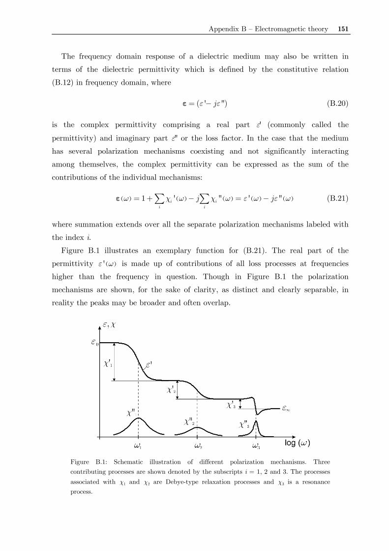
Appendix B – Electromagnetic theory 151
The frequency domain response of a dielectric medium may also be written in
terms of the dielectric permittivity which is defined by the constitutive relation
(B.12) in frequency domain, where
( )' ''jε ε= −ε (B.20)
is the complex permittivity comprising a real part ε' (commonly called the
permittivity) and imaginary part ε'' or the loss factor. In the case that the medium
has several polarization mechanisms coexisting and not significantly interacting
among themselves, the complex permittivity can be expressed as the sum of the
contributions of the individual mechanisms:
( ) ( ) ( ) ( ) ( )1 ' '' ' ''i ii i
j jω χ ω χ ω ε ω ε ω= + − = −∑ ∑ε (B.21)
where summation extends over all the separate polarization mechanisms labeled with
the index i.
Figure B.1 illustrates an exemplary function for (B.21). The real part of the
permittivity ( )'ε ω is made up of contributions of all loss processes at frequencies
higher than the frequency in question. Though in Figure B.1 the polarization
mechanisms are shown, for the sake of clarity, as distinct and clearly separable, in
reality the peaks may be broader and often overlap.
Figure B.1: Schematic illustration of different polarization mechanisms. Three contributing processes are shown denoted by the subscripts i = 1, 2 and 3. The processes associated with χ1 and χ2 are Debye-type relaxation processes and χ3 is a resonance process.

152 B.3 Debye relaxation model
B.3 Debye relaxation model
When a direct voltage applied to a dielectric for a sufficiently long duration is
suddenly removed, the decay of polarization to zero value is not instantaneous but
takes a finite time. This is the time required for the dipoles to revert to a random
distribution, in equilibrium with the temperature of the medium, from a field-oriented
alignment. Similarly, the building up of polarization following the sudden application
of a direct voltage takes also a finite time interval before the polarization attains its
maximum value. This phenomenon is described by the general term dielectric
relaxation.
Figure B.2: Transient response of a generic sample showing single relation.
In the simplest case, the polarization of a sample will relax towards the steady
state as a first-order process characterized by a single time constant τ. A typical
transient response on the application of a unit step function is given in Figure B.2.
This has the form
( ) ( )s 1 exp tD t D D Dτ∞ ∞
⎛ ⎞⎛ ⎞⎟⎜ ⎟⎜= + − − − ⎟⎟⎜ ⎜ ⎟⎟⎜ ⎝ ⎠⎝ ⎠, (B.22)
which is characterized by an instantaneous response D∞ following an exponential
growth to the static value sD . From (B.22), this relationship may also be written in
terms of permittivity
( ) ( )s 1 exp ttε ε ε ετ∞ ∞
⎛ ⎞⎛ ⎞⎟⎜ ⎟⎜= + − − − ⎟⎟⎜ ⎜ ⎟⎟⎜ ⎝ ⎠⎝ ⎠. (B.23)
Taking the Laplace transform to convert to the complex frequency (s) domain
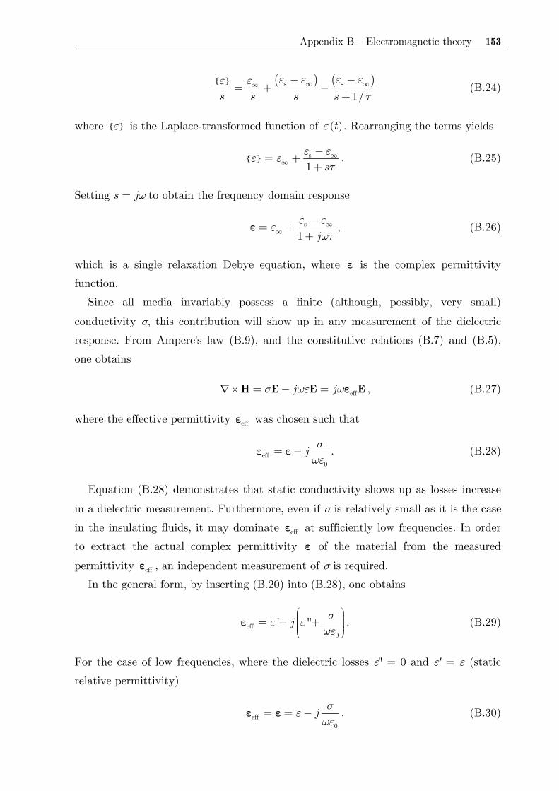
Appendix B – Electromagnetic theory 153
( ) ( )s s
1/s s s sε ε ε εε ε
τ∞ ∞∞ − −
= + −+
(B.24)
where ε is the Laplace-transformed function of ( )tε . Rearranging the terms yields
s
1 sε εε ε
τ∞
∞−= ++
. (B.25)
Setting s = jω to obtain the frequency domain response
s
1 jε εε
ωτ∞
∞−= +
+ε , (B.26)
which is a single relaxation Debye equation, where ε is the complex permittivity
function.
Since all media invariably possess a finite (although, possibly, very small)
conductivity σ, this contribution will show up in any measurement of the dielectric
response. From Ampere's law (B.9), and the constitutive relations (B.7) and (B.5),
one obtains
effj jσ ωε ω∇× = − =H E E Eε , (B.27)
where the effective permittivity effε was chosen such that
eff0
j σωε
= −ε ε . (B.28)
Equation (B.28) demonstrates that static conductivity shows up as losses increase
in a dielectric measurement. Furthermore, even if σ is relatively small as it is the case
in the insulating fluids, it may dominate effε at sufficiently low frequencies. In order
to extract the actual complex permittivity ε of the material from the measured
permittivity effε , an independent measurement of σ is required.
In the general form, by inserting (B.20) into (B.28), one obtains
eff0
' ''j σε εωε
⎛ ⎞⎟⎜ ⎟= − +⎜ ⎟⎜ ⎟⎜⎝ ⎠ε . (B.29)
For the case of low frequencies, where the dielectric losses ε'' = 0 and ε' = ε (static
relative permittivity)
eff0
j σεωε
= = −ε ε . (B.30)

154 B.3 Debye relaxation model
Here for the sake of clarity eff =ε ε . This equation was already presented in chapter 3
as (3.20).