Inequality

TRADE, GROWTH, AND POVERTY*

David Dollar and Aart Kraay

A key issue today is the effect of globalisation on inequality and poverty. Well over half thedeveloping world lives in globalising economies that have seen large increases in trade andsignificant declines in tariffs. They are catching up the rich countries while the rest of thedeveloping world is falling farther behind. Second, we examine the effects on the poor. Theincrease in growth rates leads on average to proportionate increases in incomes of the poor.The evidence from individual cases and cross-country analysis supports the view that globali-sation leads to faster growth and poverty reduction in poor countries.

Recognising the enormous benefits of open international markets, we, theundersigned economists, strongly support China’s entry into the WorldTrade Organisation. China’s entry will raise living standards in both Chinaand its trading partners. By acceding to the WTO, China will open itsborders to international competition, lock in and deepen its commitmentto economic reform, and promote economic development and freedom.

– Open letter in the New York Times, spring 2000,signed by a long list of prominent economists

Openness to international trade accelerates development: this is one of the mostwidely held beliefs in the economics profession, one of the few things on whichNobel prize winners of the both the left and the right agree. The more rapidgrowth may be a transitional effect rather than a shift to a different steady stategrowth rate but clearly the transition takes a couple of decades or more, so that it isreasonable to speak of trade openness accelerating growth, rather than merelyleading to a sudden, one-time adjustment in real income.

Why is this view so prevalent? Srinivasan and Bhagwati (1999) argue that thebest evidence in support of the openness-growth link is that ‘nuanced, in-depthanalyses of country experiences in major OECD, NBER, and IBRD projectsduring the 1960s and 1970s have shown plausibly, and taking into accountnumerous country-specific factors, that trade does seem to create, even sustain,higher growth’. (p. 6) Their paper goes on to lament the shift of the professionaway from detailed case studies in favour of cross-country growth regressions.They criticise cross-country growth regressions on a number of grounds that wewill return to, while at the same time acknowledging that such regressions cancontain useful information: ‘In fact, while such regressions can be suggestive ofnew hypotheses and be valuable aids in thinking about the issue at hand, we

* Views expressed are those of the authors and do not necessarily reflect official views of the WorldBank or its members countries. We thank Sergio Kurlat and Dennis Tao for excellent research assist-ance. An earlier draft of this paper was presented at the conference on ‘Poverty and the InternationalEconomy’, sponsored by Globkom (Parliamentary Commission for Swedish Policy on Global Develop-ment) and the World Bank, October 20–21, 2000, Stockholm. We thank Jeff Williamson, Dani Rodrik,and seminar participants for helpful comments on the initial draft.

The Economic Journal, 114 (February), F22–F49. � Royal Economic Society 2004. Published by BlackwellPublishing, 9600 Garsington Road, Oxford OX4 2DQ, UK and 350 Main Street, Malden, MA 02148, USA.

[ F22 ]

would reiterate that great caution is needed in using them at all as plausible‘‘scientific’’ support’. (p. 36).

We agree that individual cases contain important information upon whicheconomists often base their views. The systematic case studies cited by Srinivasanand Bhagwati generally concern trade liberalisation in the 1960s and 1970s. It is ashame that there has not been a similar systematic treatment of post-1980 glob-alisers. In the next Section of the paper we identify post-1980 globalisers that aregood candidates for case studies. In particular, we single out the top one-third ofdeveloping countries in terms of increases in trade to GDP over the past 20 years.1

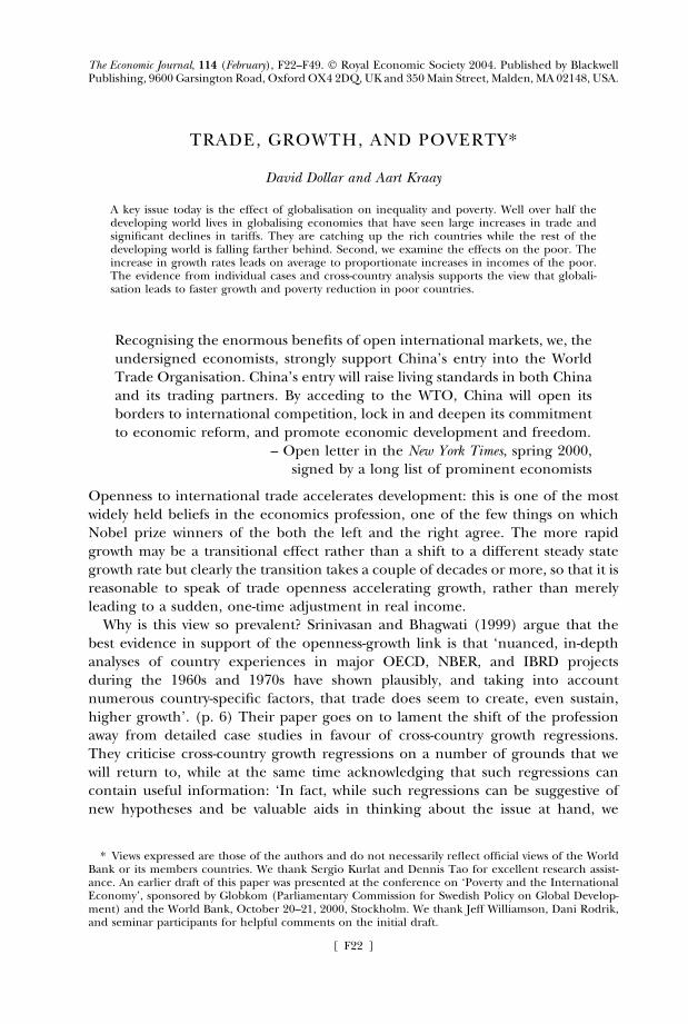
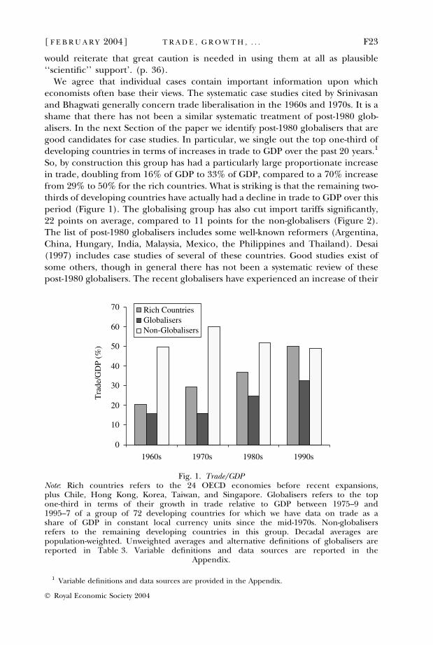
So, by construction this group has had a particularly large proportionate increasein trade, doubling from 16% of GDP to 33% of GDP, compared to a 70% increasefrom 29% to 50% for the rich countries. What is striking is that the remaining two-thirds of developing countries have actually had a decline in trade to GDP over thisperiod (Figure 1). The globalising group has also cut import tariffs significantly,22 points on average, compared to 11 points for the non-globalisers (Figure 2).The list of post-1980 globalisers includes some well-known reformers (Argentina,China, Hungary, India, Malaysia, Mexico, the Philippines and Thailand). Desai(1997) includes case studies of several of these countries. Good studies exist ofsome others, though in general there has not been a systematic review of thesepost-1980 globalisers. The recent globalisers have experienced an increase of their

0

10

20

30

40

50

60

70

1960s 1970s 1980s 1990s

Tra

de/G

DP

(%)

Rich CountriesGlobalisersNon-Globalisers

Fig. 1. Trade/GDPNote: Rich countries refers to the 24 OECD economies before recent expansions,plus Chile, Hong Kong, Korea, Taiwan, and Singapore. Globalisers refers to the topone-third in terms of their growth in trade relative to GDP between 1975–9 and1995–7 of a group of 72 developing countries for which we have data on trade as ashare of GDP in constant local currency units since the mid-1970s. Non-globalisersrefers to the remaining developing countries in this group. Decadal averages arepopulation-weighted. Unweighted averages and alternative definitions of globalisers arereported in Table 3. Variable definitions and data sources are reported in the

Appendix.

[ F E B R U A R Y 2004] F23T R A D E , G R O W T H , . . .

1 Variable definitions and data sources are provided in the Appendix.

� Royal Economic Society 2004

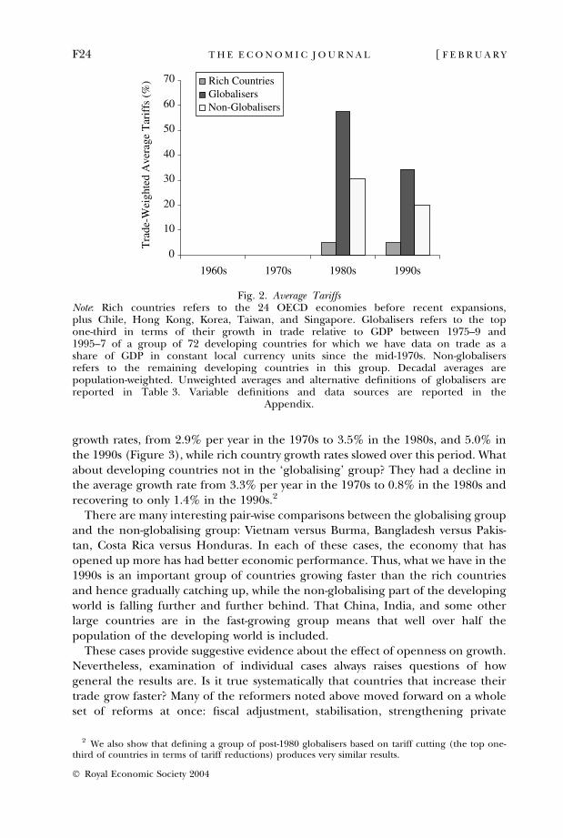
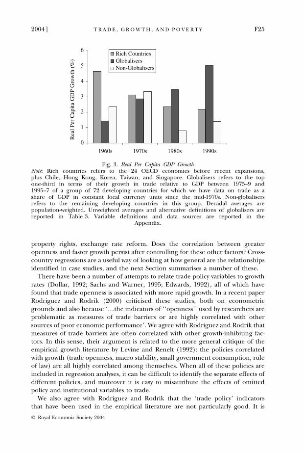
growth rates, from 2.9% per year in the 1970s to 3.5% in the 1980s, and 5.0% inthe 1990s (Figure 3), while rich country growth rates slowed over this period. Whatabout developing countries not in the ‘globalising’ group? They had a decline inthe average growth rate from 3.3% per year in the 1970s to 0.8% in the 1980s andrecovering to only 1.4% in the 1990s.2

There are many interesting pair-wise comparisons between the globalising groupand the non-globalising group: Vietnam versus Burma, Bangladesh versus Pakis-tan, Costa Rica versus Honduras. In each of these cases, the economy that hasopened up more has had better economic performance. Thus, what we have in the1990s is an important group of countries growing faster than the rich countriesand hence gradually catching up, while the non-globalising part of the developingworld is falling further and further behind. That China, India, and some otherlarge countries are in the fast-growing group means that well over half thepopulation of the developing world is included.

These cases provide suggestive evidence about the effect of openness on growth.Nevertheless, examination of individual cases always raises questions of howgeneral the results are. Is it true systematically that countries that increase theirtrade grow faster? Many of the reformers noted above moved forward on a wholeset of reforms at once: fiscal adjustment, stabilisation, strengthening private

0

10

20

30

40

50

60

70

1960s 1970s 1980s 1990s

Tra

de-W

eigh

ted

Ave

rage

Tar

iffs

(%

) Rich CountriesGlobalisersNon-Globalisers

Fig. 2. Average TariffsNote: Rich countries refers to the 24 OECD economies before recent expansions,plus Chile, Hong Kong, Korea, Taiwan, and Singapore. Globalisers refers to the topone-third in terms of their growth in trade relative to GDP between 1975–9 and1995–7 of a group of 72 developing countries for which we have data on trade as ashare of GDP in constant local currency units since the mid-1970s. Non-globalisersrefers to the remaining developing countries in this group. Decadal averages arepopulation-weighted. Unweighted averages and alternative definitions of globalisers arereported in Table 3. Variable definitions and data sources are reported in the

Appendix.

2 We also show that defining a group of post-1980 globalisers based on tariff cutting (the top one-third of countries in terms of tariff reductions) produces very similar results.

F24 [ F E B R U A R YT H E E C O N O M I C J O U R N A L


property rights, exchange rate reform. Does the correlation between greateropenness and faster growth persist after controlling for these other factors? Cross-country regressions are a useful way of looking at how general are the relationshipsidentified in case studies, and the next Section summarises a number of these.

There have been a number of attempts to relate trade policy variables to growthrates (Dollar, 1992; Sachs and Warner, 1995; Edwards, 1992), all of which havefound that trade openness is associated with more rapid growth. In a recent paperRodriguez and Rodrik (2000) criticised these studies, both on econometricgrounds and also because ‘…the indicators of ‘‘openness’’ used by researchers areproblematic as measures of trade barriers or are highly correlated with othersources of poor economic performance’. We agree with Rodriguez and Rodrik thatmeasures of trade barriers are often correlated with other growth-inhibiting fac-tors. In this sense, their argument is related to the more general critique of theempirical growth literature by Levine and Renelt (1992): the policies correlatedwith growth (trade openness, macro stability, small government consumption, ruleof law) are all highly correlated among themselves. When all of these policies areincluded in regression analyses, it can be difficult to identify the separate effects ofdifferent policies, and moreover it is easy to misattribute the effects of omittedpolicy and institutional variables to trade.

We also agree with Rodriguez and Rodrik that the ‘trade policy’ indicatorsthat have been used in the empirical literature are not particularly good. It is

0

1

2

3

4

5

6

1960s 1970s 1980s 1990s

Rea

l Per

Cap

ita G

DP

Gro

wth

(%

)

Rich CountriesGlobalisersNon-Globalisers

Fig. 3. Real Per Capita GDP GrowthNote: Rich countries refers to the 24 OECD economies before recent expansions,plus Chile, Hong Kong, Korea, Taiwan, and Singapore. Globalisers refers to the topone-third in terms of their growth in trade relative to GDP between 1975–9 and1995–7 of a group of 72 developing countries for which we have data on trade as ashare of GDP in constant local currency units since the mid-1970s. Non-globalisersrefers to the remaining developing countries in this group. Decadal averages arepopulation-weighted. Unweighted averages and alternative definitions of globalisers arereported in Table 3. Variable definitions and data sources are reported in the

Appendix.

2004] F25T R A D E , G R O W T H , A N D P O V E R T Y


hard to come up with clean measures of trade policy. In many developingcountries non-tariff barriers have been particularly pernicious – licensingschemes that amount to firm-specific planned allocations of imports. Yet ourexperience is that NTB coverage ratios do not effectively capture how severenon-tariff barriers are. Average tariff rates provide some information about tradepolicy, which we used to help identify our group of globalisers. Nevertheless,changes in average tariff rates are not very strongly correlated with changes intrade volumes.3

In our empirical work we use decade-over-decade changes in the volume of tradeas an imperfect proxy for changes in trade policy. In a data set spanning 100countries, we find that changes in growth rates are highly correlated with changesin trade volumes, controlling for lagged growth and addressing a variety ofeconometric difficulties. This approach differs from much of the existing empir-ical literature which relates growth to cross-country differences in trade volumes.Much of the cross-country variation in trade volumes reflects countries’ geo-graphical characteristics, such as their proximity to major markets, their size, orwhether they are landlocked. As a result this type of evidence tells us little aboutthe effects of trade policy on growth and, worse, it may simply reflect the effects ofgeography on growth through other channels; both these points are emphasisedby Rodriguez and Rodrik (2000). By focusing on decadal changes in growth andchanges in trade volumes we can at least be sure that our results are not driven bygeography, nor by any other unobserved country characteristic that drives bothgrowth and trade but varies little over time, such as institutional quality. Byincluding period dummies we are also able to control for shocks that are commonto all countries, such as global demand shocks or reductions in transport costs.

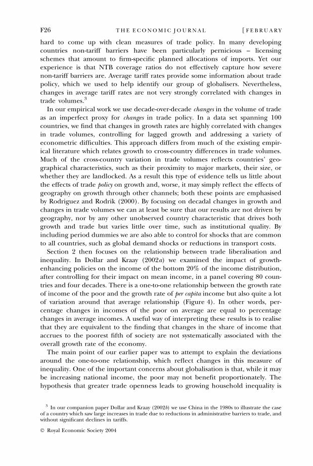
Section 2 then focuses on the relationship between trade liberalisation andinequality. In Dollar and Kraay (2002a) we examined the impact of growth-enhancing policies on the income of the bottom 20% of the income distribution,after controlling for their impact on mean income, in a panel covering 80 coun-tries and four decades. There is a one-to-one relationship between the growth rateof income of the poor and the growth rate of per capita income but also quite a lotof variation around that average relationship (Figure 4). In other words, per-centage changes in incomes of the poor on average are equal to percentagechanges in average incomes. A useful way of interpreting these results is to realisethat they are equivalent to the finding that changes in the share of income thataccrues to the poorest fifth of society are not systematically associated with theoverall growth rate of the economy.

The main point of our earlier paper was to attempt to explain the deviationsaround the one-to-one relationship, which reflect changes in this measure ofinequality. One of the important concerns about globalisation is that, while it maybe increasing national income, the poor may not benefit proportionately. Thehypothesis that greater trade openness leads to growing household inequality is

3 In our companion paper Dollar and Kraay (2002b) we use China in the 1980s to illustrate the caseof a country which saw large increases in trade due to reductions in administrative barriers to trade, andwithout significant declines in tariffs.



the hypothesis that growing openness leads to points ‘below the line’ in Figure 4:growth of income of the poor less than per capita GDP growth.

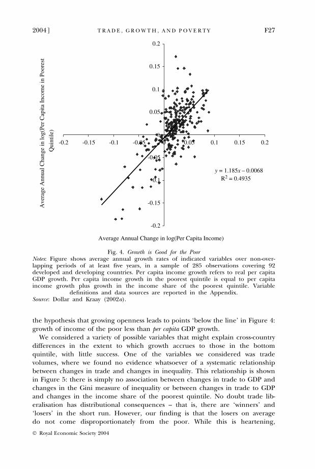
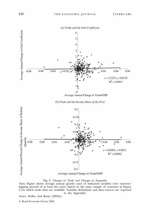
We considered a variety of possible variables that might explain cross-countrydifferences in the extent to which growth accrues to those in the bottomquintile, with little success. One of the variables we considered was tradevolumes, where we found no evidence whatsoever of a systematic relationshipbetween changes in trade and changes in inequality. This relationship is shownin Figure 5: there is simply no association between changes in trade to GDP andchanges in the Gini measure of inequality or between changes in trade to GDPand changes in the income share of the poorest quintile. No doubt trade lib-eralisation has distributional consequences – that is, there are ‘winners’ and‘losers’ in the short run. However, our finding is that the losers on averagedo not come disproportionately from the poor. While this is heartening,

y = 1.185x – 0.0068

-0.2

-0.15

-0.1

-0.05

0

0.05

0.1

0.15

0.2

-0.2 -0.15 -0.1 -0.05 0 0.05 0.1 0.15 0.2

Average Annual Change in log(Per Capita Income)

Ave

rage

Ann

ual C

hang

e in

log(

Per

Cap

ita I

ncom

e in

Poo

rest

Qui

ntile

)

R2 = 0.4935

Fig. 4. Growth is Good for the PoorNotes: Figure shows average annual growth rates of indicated variables over non-over-lapping periods of at least five years, in a sample of 285 observations covering 92developed and developing countries. Per capita income growth refers to real per capitaGDP growth. Per capita income growth in the poorest quintile is equal to per capitaincome growth plus growth in the income share of the poorest quintile. Variable

definitions and data sources are reported in the Appendix.Source: Dollar and Kraay (2002a).



(a) Trade and the Gini Coefficient

-4

-3

-2

-1

0

1

2

3

4

5

6

-0.08 -0.06 -0.04 -0.02 0 0.02 0.04 0.06 0.08

Average Annual Change in Trade/GDP

y = 0.0489x + 0.0012

-0.2

-0.15

-0.1

-0.05

0

0.05

0.15

0.2

-0.08 -0.06 -0.04 -0.02 0 0.02 0.04 0.06 0.08

Qui

ntil

e

(b) Trade and the Income Share of the Poor

Ave

rage

Ann

ual C

hang

e in

Gin

i Coe

ffic

ient

0.1

R2 = 0.0002

Average Annual Change in Trade/GDPAve

rage

Ann

ual P

erce

nt C

hang

e in

Inc

ome

Shar

e of

Bot

tom

y = 2.5227x + 0.0139

R2 = 0.0013

Fig. 5. Changes in Trade and Changes in InequalityNotes: Figure shows average annual growth rates of indicated variables over non-over-lapping periods of at least five years, based on the same sample of countries as Figure4 for which trade data are available. Variable definitions and data sources are reported

in the Appendix.Source: Dollar and Kraay (2002a).



nevertheless it has to be a concern that some poor households are hurt in theshort run by trade liberalisation. It is thus important to complement open tradepolicies with effective social protection measures such as unemployment insur-ance and food-for-work schemes.4 To the extent that trade openness raisesnational income, it strengthens the fiscal ability of a society to provide thesesafety nets.

The fact that increased trade generally goes hand-in-hand with more rapidgrowth and no systematic change in household income distribution, means thatincreased trade generally goes hand-in-hand with improvements in well-being ofthe poor. We can relate the cross-country findings on trade and inequality back tothe specific countries in our globalising group. Some have had increases inhousehold income inequality over the past 20 years, most notably China. But it isnot true in general that the liberalising economies have had increases ininequality. Costa Rica’s and the Philippines’ income distributions have been quitestable. Inequality has declined in Malaysia and Thailand. Mexico had an increasein inequality in the 1980s followed by a decline in inequality in the 1990s. Sincemost of the countries have had only relatively small changes in household incomeinequality, the growth rate of income of the poor is closely related to the growthrate of per capita GDP.

Although Vietnam is not included among our globalisers (due to limits on theavailability of data we use to identify the other globalisers), it nicely illustrates ourmain finding about trade and poverty. As Vietnam has opened up, it has had alarge increase in per capita GDP and no significant change in inequality. Thus,income of the poor has risen dramatically and the level of absolute poverty hasdropped sharply, from 75% of the population in 1988 to 37% in 1998 – poverty wascut in half in ten years! In the case of Vietnam we have particularly good data,because a representative household survey was conducted early in the reformprocess (1992–3), and then the same 5,000 households were visited again six yearslater. Of the poorest 5% of households in 1992, 98% had higher income six yearslater. Since Vietnam’s opening has resulted in exports of rice (produced by mostof the poor farmers) and labour-intensive products such as footwear, it should beno surprise that the vast majority of poor households benefited immediately from amore open trading system.

All of this work is aimed at the counterfactual question, what can we expect tohappen when developing countries liberalise trade and participate more in theglobal trading system? Obviously for a particular closed economy (say, Burma) wecannot predict with certainty what will happen. The specific outcome will dependon a whole host of factors (including the country’s factor endowments, its location,complementary policies put in place). But we can make some qualitative predic-tions. Based on the experiences of individual cases of post-1980 liberalisers and thegeneral patterns detected in cross-country regressions, it is highly probable thatBurma’s growth rate would accelerate. Furthermore, based on other countries’experiences, there is no reason to expect any large change in household income

4 Closed economies obviously need safety nets as well since households are subject to shocks frombusiness cycles, technological change, weather and disease.



inequality. Therefore, we can expect that greater openness would improve thematerial lives of the poor. We also know that there will be some individual losersamong the poor in the short run and that effective social protection can easethe transition to a more open economy, so that all of the poor benefit fromdevelopment.

1. Growth of the Post-1980 Globalisers

The objective in this Section is to identify developing countries that have significantlyopened up to foreign trade in the past 20 years and to compare their growth to that ofother developing countries that have remained more closed. We identify these post-1980 globalisers based on their growth in trade relative to GDP in constant prices andbased on their reductions in average tariff rates. Both measures have strengths andweaknesses. Trade volumes are clearly endogenous variables that reflect a wide rangeof factors other than trade policy. Across countries, a significant share of the variationin trade reflects countries’ geographical characteristics. We abstract from thesegeographical determinants of trade by focusing on proportional changes in tradevolumes relative to GDP but we recognise that growth in trade volumes may alsoreflect many factors other than trade liberalisation. We therefore also use reductionsin average tariff rates to identify globalisers. The average tariff rate is clearly a policyvariable but the relationship between tariff rates and trade volumes is not that strong.This reflects both the fact that trade volumes are determined by many factors otherthan policy and also the fact that available data on tariffs are a very imperfectmeasure of trade policy. For example, we use a dataset of unweighted average tariffs(since this gives us the best country and period coverage) which can give dispro-portionate weight to tariffs on commodities that represent a small fraction of im-ports. On the other hand, trade-weighted average tariffs give no weight to tariffs ongoods that are so high that imports are choked off entirely. Moreover, in manycountries non-tariff barriers ranging from explicit quotas and licensing schemes tolocal content requirements and health and safety standards constitute significantobstacles to trade that are not captured by average tariffs. The advantage of tradevolumes is that they in part reflect these non-tariff barriers to trade.

We begin with a group of 101 countries for which we have data on trade as ashare of GDP in constant prices beginning in the 1970s. We begin by separatingout the 24 OECD countries (before recent expansions), and add to that group fiveeconomies that we think of as early liberalisers (Chile, Hong Kong, Taiwan, Sin-gapore and South Korea). Their stories are well known, and we want to focus onthe developing countries that have opened up during the recent wave of globali-sation in the 1980s and 1990s. This expanded group of rich countries provides auseful benchmark against which to measure the experience of the globalising andnon-globalising developing countries. With these wealthy countries put aside, wehave trade data for 73 developing economies.5

5 We do not have constant local currency trade to GDP ratios for Turkey, an OECD member, for the1970s. This is why the 29 rich countries and the 73 developing countries do not add up to the total of101 countries.



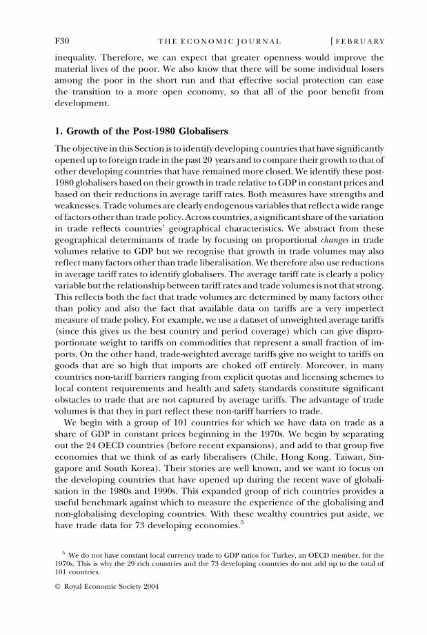
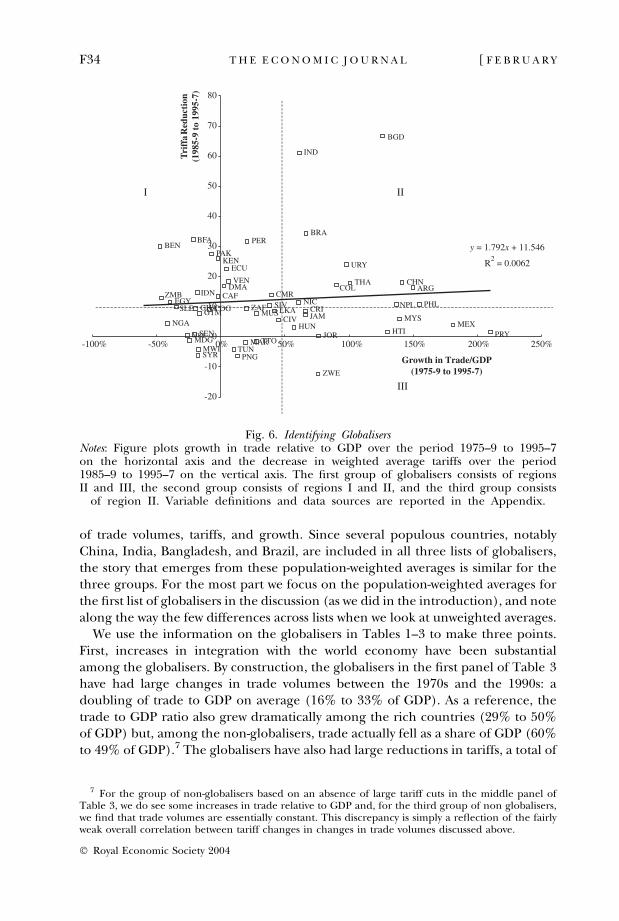
Our first group of globalisers is based on the top one-third of these developingcountries in terms of their growth in trade as a share of GDP at constant pricesbetween 1975–9 and 1995–7. These countries are shown in Table 1, and includesome well-known economic reformers: Malaysia and Thailand in East Asia, whichliberalised trade in the early 1980s; China, which has been liberalising tradethroughout this period; Bangladesh and India in South Asia, with reforms more inthe 1990s; and several Latin American economies (notably, Argentina, Brazil, andMexico). We have highlighted the experience of this group of globalisers in theintroduction to the paper. However, there are a couple of countries on the list thatstrike us as anomalies (for example, Haiti and Rwanda). Their inclusion remindsus of the problem that we noted earlier, that a large increase in trade might reflectnon-trade-policy factors such as cessation of civil war.6

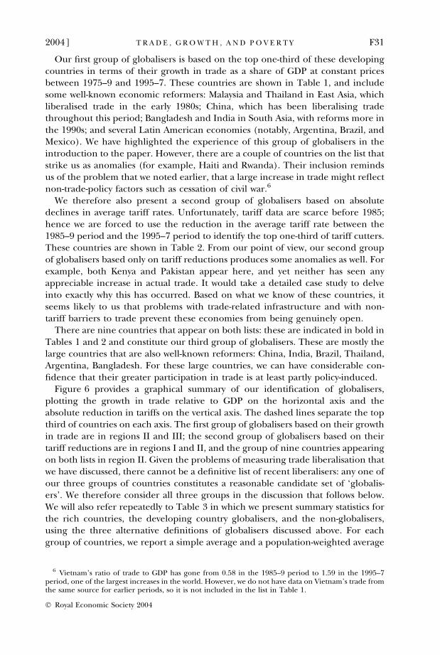
We therefore also present a second group of globalisers based on absolutedeclines in average tariff rates. Unfortunately, tariff data are scarce before 1985;hence we are forced to use the reduction in the average tariff rate between the1985–9 period and the 1995–7 period to identify the top one-third of tariff cutters.These countries are shown in Table 2. From our point of view, our second groupof globalisers based only on tariff reductions produces some anomalies as well. Forexample, both Kenya and Pakistan appear here, and yet neither has seen anyappreciable increase in actual trade. It would take a detailed case study to delveinto exactly why this has occurred. Based on what we know of these countries, itseems likely to us that problems with trade-related infrastructure and with non-tariff barriers to trade prevent these economies from being genuinely open.

There are nine countries that appear on both lists: these are indicated in bold inTables 1 and 2 and constitute our third group of globalisers. These are mostly thelarge countries that are also well-known reformers: China, India, Brazil, Thailand,Argentina, Bangladesh. For these large countries, we can have considerable con-fidence that their greater participation in trade is at least partly policy-induced.

Figure 6 provides a graphical summary of our identification of globalisers,plotting the growth in trade relative to GDP on the horizontal axis and theabsolute reduction in tariffs on the vertical axis. The dashed lines separate the topthird of countries on each axis. The first group of globalisers based on their growthin trade are in regions II and III; the second group of globalisers based on theirtariff reductions are in regions I and II, and the group of nine countries appearingon both lists in region II. Given the problems of measuring trade liberalisation thatwe have discussed, there cannot be a definitive list of recent liberalisers: any one ofour three groups of countries constitutes a reasonable candidate set of ‘globalis-ers’. We therefore consider all three groups in the discussion that follows below.We will also refer repeatedly to Table 3 in which we present summary statistics forthe rich countries, the developing country globalisers, and the non-globalisers,using the three alternative definitions of globalisers discussed above. For eachgroup of countries, we report a simple average and a population-weighted average

6 Vietnam’s ratio of trade to GDP has gone from 0.58 in the 1985–9 period to 1.59 in the 1995–7period, one of the largest increases in the world. However, we do not have data on Vietnam’s trade fromthe same source for earlier periods, so it is not included in the list in Table 1.



Tab

le1

Pos

t-1980

Glo

bali

sers

(Bas

edo

nIn

crea

ses

inT

rad

eV

olu

mes

)

Ave

rage

ann

ual

per

cap

ita

GD

Pgr

ow

th(%

)A

vera

getr

ade/

GD

P(%

)W

eigh

ted

aver

age

tari

ffra

te

1970

s19

75s

1980

s19

85s

1990

s19

95s

1970

s19

75s

1980

s19

85s

1990

s19

95s

1985

s19

90s

1995

s

Arg

enti

na

2.3

1.0

)3.

2)

2.0

6.8

5.2

11.3

13.2

16.4

15.5

23.7

32.9

27.5

13.9

11.0

Ban

glad

esh

)7.

03.

21.

23.

13.

43.

710

.311

.813

.814

.018

.626

.792

.754

.326

.0B

razi

l8.

83.

8)

2.9

1.5

0.9

1.6

11.1

10.7

10.3

10.5

13.5

17.9

45.8

21.0

11.5

Ch

ina

1.4

3.4

3.9

1.7

8.6

7.8

12.5

14.1

26.7

28.5

30.1

34.2

38.8

39.9

20.9

Co

lom

bia

4.0

3.5

0.0

2.5

2.4

0.6

33.8

30.9

33.4

33.1

45.0

58.9

29.4

16.6

12.2

Co

sta

rica

3.4

3.6

)3.

62.

02.

0)

0.1

74.5

77.1

71.3

82.0

108.

312

8.1

19.5

12.6

11.2

Do

min

ican

Rep

.7.

61.

7)

2.1

3.5

1.8

5.6

38.7

31.5

41.3

40.3

56.3

92.3

–17

.816

.2H

aiti

1.4

3.4

)3.

4)

2.2

)7.

3)

0.3

32.2

43.0

47.7

50.8

67.0

98.9

11.6

–10

.0H

un

gary

5.9

2.8

1.2

1.4

)2.

83.

340

.947

.148

.452

.757

.674

.018

.09.

914

.8In

dia

)1.

20.

73.

34.

12.

64.

412

.713

.715

.916

.317

.022

.199

.461

.938

.3Iv

ory

coas

t1.

65.

1)

3.8

)3.

6)

3.4

3.3

54.4

52.7

70.4

67.5

68.0

76.4

26.3

23.8

20.7

Jam

aica

2.5

)3.

8)

0.1

3.4

)0.

8)

2.7

80.0

75.9

76.5

106.

610

9.2

125.

918

.419

.610

.9Jo

rdan

8.2

10.8

1.1

)4.

31.

4)

1.6

–94

.211

8.2

104.

016

2.2

166.

216

.315

.816

.0M

alay

sia

6.5

6.6

3.8

3.0

5.8

5.4

89.3

91.7

106.

812

0.8

173.

921

9.8

14.9

14.3

8.9

Mal

i0.

84.

5)

1.3

1.1

)1.

82.

328

.629

.942

.851

.351

.651

.3–

–18

.8M

exic

o4.

53.

3)

2.3

)0.

22.

44.

217

.017

.721

.223

.233

.549

.916

.712

.812

.8N

epal

0.7

11.0

1.0

2.0

3.0

2.2

16.5

25.4

31.0

32.2

42.0

60.3

21.8

16.1

11.0

Nic

arag

ua

2.7

)9.

80.

5)

7.5

)2.

2–

49.1

52.9

65.6

51.0

68.5

85.1

22.1

12.7

10.7

Par

agu

ay3.

75.

2)

4.2

)0.

71.

0)

0.2

28.2

32.1

32.0

37.8

77.3

99.4

10.9

13.1

9.3

Ph

ilip

pin

es3.

13.

3)

3.1

2.9

)0.

63.

140

.541

.652

.256

.275

.510

6.1

27.8

24.5

17.2

Rw

and

a)

0.9

2.8

0.4

)1.

5)

14.9

0.3

19.1

22.9

26.4

29.5

46.5

37.4

33.0

38.4

–T

hai

lan

d1.

86.

23.

06.

96.

01.

547

.447

.149

.859

.184

.694

.641

.036

.623

.1U

rugu

ay0.

12.

8)

6.3

4.1

4.9

4.3

35.5

42.6

47.3

50.0

66.4

84.3

33.7

18.9

9.6

Zim

bab

we

5.8

)3.

10.

0)

0.9

0.4

3.1

–43

.844

.244

.859

.477

.19.

217

.221

.5

Not

es:

Var

iab

led

efin

itio

ns

and

dat

aso

urc

esar

ere

po

rted

inth

eA

pp

end

ix.



Tab

le2

Pos

t-1980

Glo

bali

sers

(Bas

edo

nR

edu

ctio

ns

inT

arif

fs)

Co

un

try

Ave

rage

ann

ual

per

cap

ita

GD

Pgr

ow

th(%

)A

vera

getr

ade/

GD

P(%

)W

eigh

ted

aver

age

tari

ffra

te

1970

s19

75s

1980

s19

85s

1990

s19

95s

1970

s19

75s

1980

s19

85s

1990

s19

95s

1985

s19

90s

1995

s

Arg

enti

na

2.3

1.0

)3.

2)

2.0

6.8

5.2

11.3

13.2

16.4

15.5

23.7

32.9

27.5

13.9

11.0

Ban

glad

esh

)7.

03.

21.

23.

13.

43.

710

.311

.813

.814

.018

.626

.792

.754

.326

.0B

enin

)0.

20.

1)

1.9

)4.

61.

42.

678

.787

.288

.763

.951

.845

.842

.841

.012

.7B

razi

l8.

83.

8)

2.9

1.5

0.9

1.6

11.1

10.7

10.3

10.5

13.5

17.9

45.8

21.0

11.5

Bu

rkin

aF

aso

1.2

2.6

0.9

1.2

)0.

93.

242

.448

.148

.546

.143

.137

.960

.8–

28.5

Cam

ero

on

2.9

5.5

4.0

)2.

2)

7.2

2.1

53.6

46.7

59.3

61.3

68.5

65.0

32.0

18.6

18.1

Cen

tral

Afr

.R)

0.9

0.9

)3.

2)

1.9

)2.

8)

0.2

40.7

43.1

48.1

44.3

46.9

42.1

32.0

–18

.6C

hin

a1.

43.

43.

91.

78.

67.

812

.514

.126

.728

.530

.134

.238

.839

.920

.9C

olo

mb

ia4.

0)

3.5

0.0

2.5

2.4

0.6

33.8

30.9

33.4

33.1

45.0

58.9

29.4

16.6

12.2

Do

min

ica

––

5.7

5.9

1.4

1.8

–10

9.6

108.

911

4.5

118.

511

2.3

31.9

28.0

15.0

Ecu

ado

r8.

34.

0)

2.8

)1.

11.

10.

649

.854

.946

.947

.052

.557

.534

.310

.611

.7E

gyp

t0.

34.

13.

7)

0.6

0.1

3.3

84.0

98.7

83.6

64.6

61.6

59.7

39.7

35.3

28.1

Eth

iop

ia0.

30.

8)

0.3

1.9

)1.

25.

0–

–27

.728

.622

.925

.429

.628

.816

.3In

dia

)1.

20.

73.

34.

12.

64.

412

.713

.715

.916

.317

.022

.199

.461

.938

.3In

do

nes

ia5.

55.

65.

72.

54.

34.

558

.069

.460

.148

.650

.257

.027

.920

.113

.2K

enya

9.2

2.7

)2.

23.

5)

0.6

0.6

109.

579

.956

.651

.460

.778

.239

.433

.313

.5N

icar

agu

a2.

7)

9.8

0.5

)7.

5)

2.2

–49

.152

.965

.651

.068

.585

.122

.112

.710

.7P

akis

tan

)2.

43.

32.

12.

50.

8)

0.3

47.6

37.1

35.7

33.4

34.9

34.5

69.2

59.8

41.7

Per

u3.

4)

3.1

)2.

8)

3.3

2.7

3.0

47.0

43.7

45.3

37.8

44.3

52.7

45.0

19.0

13.3

Th

aila

nd

1.8

6.2

3.0

6.9

6.0

1.5

47.4

47.1

49.8

59.1

84.6

94.6

41.0

36.6

23.1

Uga

nd

a)

0.8

)1.

91.

90.

41.

64.

2–

–35

.337

.831

.443

.125

.017

.113

.0U

rugu

ay0.

12.

8)

6.3

4.1

4.9

4.3

35.5

42.6

47.3

50.0

66.4

84.3

33.7

18.9

9.6

Ven

ezu

ela

)1.

12.

2)

3.7

)1.

32.

30.

261

.451

.542

.642

.847

.254

.731

.115

.812

.7Z

amb

ia2.

0)

6.9

)4.

0)

1.7

)1.

42.

419

4.2

145.

898

.387

.678

.978

.329

.926

.417

.0

Not

es:

Var

iab

led

efin

itio

ns

and

dat

aso

urc

esar

ere

po

rted

inth

eA

pp

end

ix.



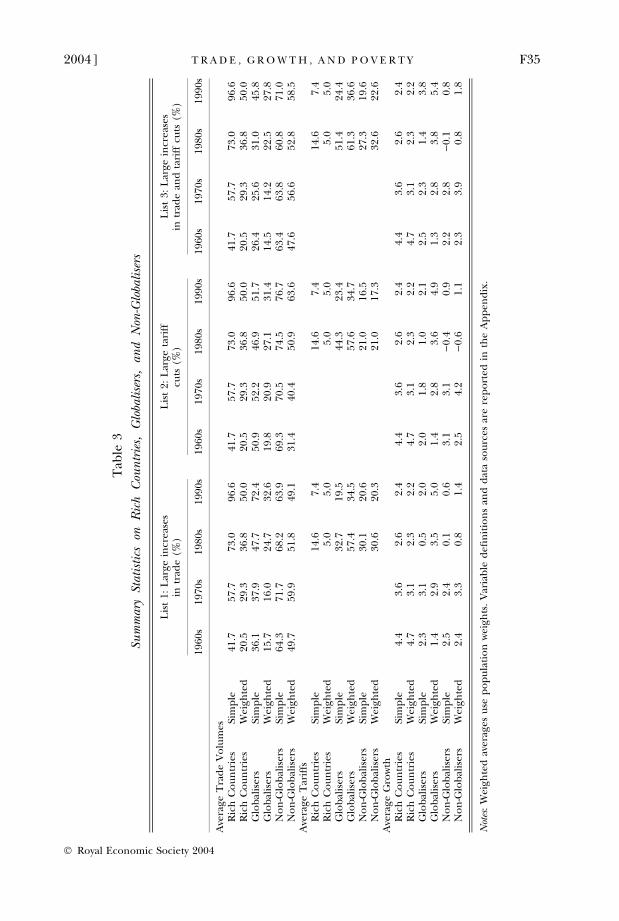
of trade volumes, tariffs, and growth. Since several populous countries, notablyChina, India, Bangladesh, and Brazil, are included in all three lists of globalisers,the story that emerges from these population-weighted averages is similar for thethree groups. For the most part we focus on the population-weighted averages forthe first list of globalisers in the discussion (as we did in the introduction), and notealong the way the few differences across lists when we look at unweighted averages.

We use the information on the globalisers in Tables 1–3 to make three points.First, increases in integration with the world economy have been substantialamong the globalisers. By construction, the globalisers in the first panel of Table 3have had large changes in trade volumes between the 1970s and the 1990s: adoubling of trade to GDP on average (16% to 33% of GDP). As a reference, thetrade to GDP ratio also grew dramatically among the rich countries (29% to 50%of GDP) but, among the non-globalisers, trade actually fell as a share of GDP (60%to 49% of GDP).7 The globalisers have also had large reductions in tariffs, a total of

ZWE

ZMB

ZAF

VEN

URY

TUNTTO

THA

SYR

SIVSLE

SEN PRY

PNG

PHL

PER

PAK

NPLNIC

NGAMYS

MWI

MUS

MRT

MEX

MDG MAR

LKA

KEN

JOR

JAM

IND

IDN

HUNHTI

GTMGHA

EGY

ECU

DMA

CRI

COL

COG

CMR

CIV

CHN

CAF

BRA

BGD

BFABEN

ARG

y = 1.792x + 11.546

R2 = 0.0062

-20

-10

0

10

20

30

40

50

60

70

80

-100% -50% 0% 50% 100% 150% 200% 250%

Growth in Trade/GDP(1975-9 to 1995-7)

Tri

ffa

Red

ucti

on(1

985-

9 to

199

5-7)

III

III

Fig. 6. Identifying GlobalisersNotes: Figure plots growth in trade relative to GDP over the period 1975–9 to 1995–7on the horizontal axis and the decrease in weighted average tariffs over the period1985–9 to 1995–7 on the vertical axis. The first group of globalisers consists of regionsII and III, the second group consists of regions I and II, and the third group consists

of region II. Variable definitions and data sources are reported in the Appendix.

7 For the group of non-globalisers based on an absence of large tariff cuts in the middle panel ofTable 3, we do see some increases in trade relative to GDP and, for the third group of non globalisers,we find that trade volumes are essentially constant. This discrepancy is simply a reflection of the fairlyweak overall correlation between tariff changes in changes in trade volumes discussed above.



Tab

le3

Sum

mar

ySt

atis

tics

onR

ich

Cou

ntr

ies,

Glo

bali

sers

,an

dN

on-G

loba

lise

rs

Lis

t1:

Lar

gein

crea

ses

intr

ade

(%)

Lis

t2:

Lar

geta

riff

cuts

(%)

Lis

t3:

Lar

gein

crea

ses

intr

ade

and

tari

ffcu

ts(%

)

1960

s19

70s

1980

s19

90s

1960

s19

70s

1980

s19

90s

1960

s19

70s

1980

s19

90s

Ave

rage

Tra

de

Vo

lum

esR

ich

Co

un

trie

sSi

mp

le41

.757

.773

.096

.641

.757

.773

.096

.641

.757

.773

.096

.6R

ich

Co

un

trie

sW

eigh

ted

20.5

29.3

36.8

50.0

20.5

29.3

36.8

50.0

20.5

29.3

36.8

50.0

Glo

bal

iser

sSi

mp

le36

.137

.947

.772

.450

.952

.246

.951

.726

.425

.631

.045

.8G

lob

alis

ers

Wei

ghte

d15

.716

.024

.732

.619

.820

.927

.131

.414

.514

.222

.527

.8N

on

-Glo

bal

iser

sSi

mp

le64

.371

.768

.263

.969

.370

.574

.576

.763

.463

.860

.871

.0N

on

-Glo

bal

iser

sW

eigh

ted

49.7

59.9

51.8

49.1

31.4

40.4

50.9

63.6

47.6

56.6

52.8

58.5

Ave

rage

Tar

iffs

Ric

hC

ou

ntr

ies

Sim

ple

14.6

7.4

14.6

7.4

14.6

7.4

Ric

hC

ou

ntr

ies

Wei

ghte

d5.

05.

05.

05.

05.

05.

0G

lob

alis

ers

Sim

ple

32.7

19.5

44.3

23.4

51.4

24.4

Glo

bal

iser

sW

eigh

ted

57.4

34.5

57.6

34.7

61.3

36.6

No

n-G

lob

alis

ers

Sim

ple

30.1

20.6

21.0

16.5

27.3

19.6

No

n-G

lob

alis

ers

Wei

ghte

d30

.620

.321

.017

.332

.622

.6A

vera

geG

row

thR

ich

Co

un

trie

sSi

mp

le4.

43.

62.

62.

44.

43.

62.

62.

44.

43.

62.

62.

4R

ich

Co

un

trie

sW

eigh

ted

4.7

3.1

2.3

2.2

4.7

3.1

2.3

2.2

4.7

3.1

2.3

2.2

Glo

bal

iser

sSi

mp

le2.

33.

10.

52.

02.

01.

81.

02.

12.

52.

31.

43.

8G

lob

alis

ers

Wei

ghte

d1.

42.

93.

55.

01.

42.

83.

64.

91.

32.

83.

85.

4N

on

-Glo

bal

iser

sSi

mp

le2.

52.

40.

10.

63.

13.

1)

0.4

0.9

2.2

2.8

)0.

10.

8N

on

-Glo

bal

iser

sW

eigh

ted

2.4

3.3

0.8

1.4

2.5

4.2

)0.

61.

12.

33.

90.

81.

8

Not

es:

Wei

ghte

dav

erag

esu

sep

op

ula

tio

nw

eigh

ts.

Var

iab

led

efin

itio

ns

and

dat

aso

urc

esar

ere

po

rted

inth

eA

pp

end

ix.



22% (from 57% to 35%), while tariff cuts among the non-globalising developingcountries were a much more modest 11% (from 31% to 20%).8

The second point we want to emphasise is that per capita growth rates have in-creased among the globalising economies in the 1990s relative to the 1980s. Of the24 countries in Table 1, 18 experienced an increase of growth between the 1980–4period and the 1995–7 period. Some of the increases were very large: Argentina, 8.4percentage points of growth; China, 3.9; Dominican Republic, 7.7; Mexico, 6.5; andthe Philippines, 6.2, just to highlight a few of the more successful examples. For thefirst list of globalisers, the simple average growth rate during the whole decade of the1990s increased from 0.5% to 2.0% per year relative to the 1980s. Growth in the restof the developing world increased from 0.1% per year during the ‘lost decade’ of the1980s to a scant 0.6% per year during the 1990s, while growth in the rich countriesslowed from 2.6% to 2.4%.9 It would be naı̈ve to assert that all of this improvement ingrowth should be attributed to the greater openness of these globalising economies:all of them have been engaged in wide-ranging economic reforms covering tradeand other areas. The experiences of China, Hungary, India, and Vietnam are cov-ered in Desai (1997); these countries strengthened private property rights andcarried out other reforms during this period. Virtually all of the Latin Americancountries included in the grouping stabilised high inflation and adjusted fiscallyover this period. Disentangling the particular role of trade is something we attemptin the next Section of the paper – here we simply note that trade reforms have gonehand-in-hand with other reforms and the improvements in growth during the 1990sreflect the confluence of all of these reforms.

The third point we want to make concerns the consequences of this rapidgrowth among the globalisers for worldwide income inequality across individuals.While the simple average growth rate discussed above indicates what has beenhappening to the typical globalising economy, population-weighted averagegrowth rates capture the effects on worldwide interpersonal income inequality.These population-weighted averages tell a striking story. First, the rich countrieswere growing quite rapidly in the 1960s (4.7%) and 1970s (3.1%) but their growthrates have declined over time, to 2.3% and 2.2% in the 1980s and 1990s. Withinthis group, the US growth rate has been relatively stable over four decades butduring the 1960s and 1970s Western Europe, Japan and the Asian tigers – all ofwhom were well behind the US in 1960 – grew rapidly and ‘converged’ on the US.This process of convergence has been a force for declining inequality among therich countries.

It is often argued that developing countries – most of whom had restrictedtrade regimes – did well during the 1960s and 1970s.10 However, the post-1980

8 Not surprisingly, the average tariff declines in the globalisers relative to the non-globalisers are evenmore pronounced if one considers the group of globalisers based on tariffs cuts alone, or on both tariffcuts and increases in trade volumes, in the last two panels of Table 3.

9 A quick look at Table 3 confirms that this pattern of larger improvements in growth among theglobalisers relative to the nonglobalisers holds for all three groups of globalisers and for boththe weighted and unweighted averages.

10 For example, Rodrik (1999) argues that ‘The import substitution policies followed in much of thedeveloping world until the 1980’s were quite successful in some regards and their costs have been vastlyexaggerated’ (p. 64).



globalisers did not do particularly well as a group in the 1960s (1.4% per capitagrowth) and the 1970s (2.9%). In particular, the two biggest developing countries –China and India – did not do well with import-substituting regimes in that period.For the twenty years from 1960 to 1979, the post-1980 globalisers were falling furtherand further behind the rich countries. The rest of the developing world did some-what better in the 1960s (2.4%) and 1970s (3.3%) but did little to catch up with therich countries. In the past 20 years growth rates for the rich countries slowed down;growth rates for the non-globalising developing world slowed down disastrously (to0.8% in the 1980s and only 1.4% in the 1990s); while the growth rate for the post-1980 globalisers accelerated to 3.5% per capita in the 1980s and 5.0% in the 1990s.11

Thus, in the 1990s, a very significant part of the developing world – the economiesthat opened – has begun to grow faster than the rich countries, creating animportant trend toward growing equality among open countries.12

The story that emerges so far is that developing countries that have reducedtrade barriers and traded more over the past twenty years have also grown faster.However, it is important to examine whether these relationships are true in gen-eral or depend on the particular sample of countries that we identified as ‘post-1980 globalisers’. There is after all a certain ad hoc character to how we groupcountries. We next turn to a more systematic cross-country statistical analysis oftrade and growth using regression analysis. In a companion paper (Dollar andKraay, 2002b), we extend this regression analysis in a number of dimensions.

We certainly are not the first to apply this approach to this question. During the1990s, an immense empirical growth literature has developed, which regressesgrowth in real per capita GDP on its initial level and a wide variety of controlvariables of interest. Within this literature many papers have included variousmeasures of trade or trade policy among these control variables. Many of thesepapers found significant positive correlations across countries between growth andtrade volumes or trade policies, controlling for other factors. These studies havebeen influential in reinforcing the consensus among many economists that ‘tradeis good for growth’. Recently however there has been criticism of the robustness ofthese results (Levine and Renelt, 1992; Rodriguez and Rodrik, 2000; Srinivasanand Bhagwati, 1999), which suggests a need to revisit some of these earlier results.

We estimate the following ‘standard’ growth regression:

yct ¼ b0 þ b1yc;t�k þ b02Xct þ gc þ ct þ vct ð1Þ

where yct is log-level of per capita GDP in country c at time t, yc,t)k is its lag k years ago(k ¼ 10 years in our application using decadal data) and Xct is a set of controlvariables which are measured as averages over the decade between t ) k and t.

11 This pattern of higher levels and greater increases in growth among the globalisers relative to thenon-globalisers holds for all three groups of globalisers. Moreover, it is worth noting that our sample ofnon-globalisers does not include the transition economies of Eastern Europe and the Former SovietUnion (since we did not have data on trade going back to the 1970s on which to select the ‘globalisers’).If these countries and their weak performance in the 1990s were included among the non-globalisers,then the difference in growth performance between the globalisers and the non-globalisers would beeven more stark.

12 This observation is consistent with the more systematic evidence in Ades and Glaeser (1999) whofind that poor initially open economies tend to grow faster than poor initially closed economies.



Many studies include trade volumes (exports plus imports as a share of GDP)among the variables in X. Subtracting lagged income from both sides of theequation gives the more conventional formulation in which the dependentvariable is growth, regressed on initial income and a set of control variables. Thedisturbance term in the regression consists of an unobserved country effect that isconstant over time, gc, an unobserved period effect that is common acrosscountries, ct, and a component that varies across both countries and years whichwe assume to be uncorrelated over time, mct.

Most of the empirical growth literature considers growth over a very long period(k ¼ 25 years or more) so that there is only one observation per country. As aresult, all of the effects of interest are estimated using only the cross-countryvariation in the data. Some papers consider shorter periods such as decades orquinquennia, and typically combine the cross-country and within-country variationin the data in a fairly ad-hoc manner. Caselli et al. (1996) provide a useful critiqueof conventional panel growth econometrics and a proposed solution. We adopttheir preferred estimation strategy, which is to estimate (1) in differences, usingappropriate lags of the right-hand side variables as instruments. In particular, theyadvocate estimating the following regression:

yct � yc;t�k ¼ b1ðyc;t�k � yc;t�2kÞ þ b02ðXct � Xc;t�kÞ þ ðct � ct�kÞ þ ðmct � mc;t�kÞ: ð2Þ

This is nothing more than a regression of growth on lagged growth and onchanges in the set of explanatory variables. Or, subtracting lagged growthfrom both sides of the equation, we have changes in growth from one decadeto the next as a function of initial growth and changes in the explanatoryvariables.13

This approach has several desirable features for us. While cross-country differ-ences in trade volumes are arguably a poor measure of cross-country differences intrade policy (since they to a large extent reflect geography), changes in tradevolumes within countries over time are not subject to this particular measurementproblem since countries’ geographical characteristics do not change over time.While change in trade volumes may reflect a variety of factors, we can at least bereasonably confident that geography is not one of them. Also, many of the possibleomitted variables in a growth regression that may be correlated with trade, such asrule of law, a country’s ethnic makeup, or its colonial history, change very littleover time. Again, by differencing we can at least be sure that the estimated coef-ficient on trade is not simply picking up a correlation with these omitted time-invariant country characteristics. A further advantage of this differenced growthequation is that it presents a natural set of instruments to control for the possibleproblem of reverse causation from growth to trade. Our identifying assumption isthat while trade volumes may be correlated with the contemporaneous and laggedshocks to GDP growth (E[Xctvc,t)s] „ 0 for s ‡ 0), they are uncorrelated with future

13 Elaborations of these techniques involve jointly estimating a system of two equations, in levels (1)and in differences (2), and using lagged changes of endogenous variables as instruments for levels inthe former (Arellano and Bover, 1995). This approach can yield important efficiency gains (Blundelland Bond, 1998) but is less appropriate in our application where we want to identify the effects ofinterest using within country changes in growth.



shocks to GDP growth, (E[Xctvc,t+s] ¼ 0 for s > 0). In practice, this means thatwhen we regress growth in the 1990s on growth in the 1980s and the change intrade volumes between the 1980s and 1990s, we can use the level of trade volumesin the 1970s as an instrument for trade openness.14

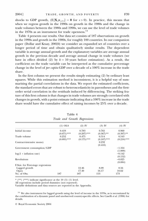
Table 4 presents our results. Our data set consists of 187 observations on growthin the 1990s and growth in the 1980s, for roughly 100 countries. In our companionpaper (Dollar and Kraay, 2002b) we consider an expanded set of countries over alonger period of time and obtain qualitatively similar results. The dependentvariable is average annual growth and the explanatory variables are average annualgrowth in the previous decade and average annual change in trade volumes (wehave in effect divided (2) by k ¼ 10 years before estimation). As a result, thecoefficient on the trade variable can be interpreted as the cumulative percentagechange in the level of per capita GDP over a decade of a 100% increase in the tradeshare.

In the first column we present the results simply estimating (2) by ordinary leastsquares. While this estimation method is inconsistent, it is a helpful way of sum-marising the partial correlations in the data. We report the estimated coefficients,the standard errors that are robust to heteroscedasticity in parentheses and the first-order serial correlation in the residuals induced by differencing. The striking fea-ture of this first column is that changes in trade volumes are strongly correlated withchanges in growth, with a point estimate indicating that a 100% increase in the tradeshare would have the cumulative effect of raising incomes by 25% over a decade.

Table 4

Trade and Growth Regressions

(1) OLS (2) IV (3) IV (4) IV

Initial income 0.419 0.783 0.765 0.960(0.071)*** (0.297)*** (0.367)** (0.397)**

Trade volume 0.252 0.475 0.514 0.543(0.095)*** (0.175)*** (0.187)*** (0.210)***

Contract-intensive money 0.232(0.410)

Government consumption/GDP )1.164(1.009)

log(1 + inflation rate) )0.142(0.152)

Revolutions )0.025(0.084)

F-Stat. for First-stage regressionsLagged growth 12.46 8.09 8.56Open 17.49 16.17 10.62

No. of Obs. 187 187 153 173

* (**) (***) indicate significance at the 10 (5) (1) level.All regressions include period dummies (not reported).Variable definitions and data sources are reported in the Appendix.

14 We also instrument for lagged growth using the level of income in the 1970s, as is necessitated bythe combination of a dynamic panel and unobserved country-specific effects. See Caselli et al. (1996) fordetails.



Of more interest are the results in the second column, where we instrumentfor initial income and trade volumes as described above. The coefficient ontrade jumps to 0.48 and remains highly significant. It is worth reiterating thatthese estimates reflect the effect of changes in trade on changes in growth. As aresult, they do not reflect the effect of geography-induced differences in trade,as in the paper by Frankel and Romer (1999), nor are they tainted by theomission of any variables that matter for growth but change little over time.Our instrumentation strategy also address the possibility of reverse causationfrom growth to trade. Furthermore, as long as any time-varying omitted vari-ables are uncorrelated with the level of trade openness two decades before,our instrumented coefficients will not reflect the spurious omission of thesevariables.

One possible explanation for the apparent effect of trade on growth is that itreflects institutional quality which is omitted from the regression (Rodrik, 2000).According to this argument, improvements in institutional quality make coun-tries more attractive as trading partners and also have direct effects on growth.This argument is neither implausible, nor is it inconsistent with trade also havinga direct effect on growth. In (Dollar and Kraay, 2002b) we examine this hypo-thesis empirically in detail and find little support for the idea that the partialcorrelation between trade and growth is driven by the omitted effect of institu-tional quality. In column 3 of Table 4, we show one such result in this sample ofcountries. We measure institutional quality using one of the few time-varyingproxies for institutional quality that are available back to the 1970s. In particular,we use one minus the ratio of currency in circulation to M2. This variable,coined as ‘contract-intensive money’ by Clague et al. (1999) measures the extentto which property rights are sufficiently secure that individuals are willing to holdliquid assets via financial intermediaries. These authors document a strongpositive cross-country relationship between this variable and both investment andgrowth. We find however that changes in this variable have little explanatorypower for changes in growth over time, as it enters positively but insignificantly.More important for our purposes, our basic result on the importance of trade forgrowth remains positive and highly significant, and even becomes slightly largerin magnitude than in column 2. In our companion paper we find that thisgeneral conclusion holds when we consider several other measures of institu-tional quality, including the widely-used subjective measures produced by theInternational Country Risk Guide and Freedom House, as well as measures ofviolent strife. Taken together, these results suggest to us that omitted changes ininstitutional quality are unlikely to be driving the observed partial correlationbetween trade and growth.

In column 4 of Table 4 we show that the results are also robust to the inclusionof other policy and non-policy determinants of growth, suggesting that the effectsof trade are also not simply capturing the overall quality of the growth environ-ment. We also note that our strategy of using internal instruments to addresspotential problems of endogeneity appears to work reasonably well. In Table 4, wereport the F-statistics for the first-stage regressions for lagged growth andopenness. In all cases the null hypothesis of zero slopes is overwhelmingly



rejected.15 In summary, we argue that the experience of the post-1980 globalisersillustrates a more general finding, that greater involvement in trade is related tofaster growth in developing countries.

2. Inequality and Poverty in the Post-1980 Globalisers

Globalisation has dramatically increased inequality between and withinnations.

– Jay Mazur, ‘Labor’s new internationalism’,Foreign Affairs, January/February 2000

One of the most common populist views of growing international economicintegration is that it leads to growing inequality between nations – that is, thatglobalisation causes divergence between rich and poor countries – and withinnations – that is, that it benefits richer households proportionally more than itbenefits poorer ones. In the previous Section of this paper we have argued thatthe experience of globalisers shows how greater openness to international tradehas in fact contributed to narrowing the gap between rich and poor countries,as the globalisers have grown faster than the rich countries as a group. In thisSection of the paper we turn to the effects of globalisation on inequality withincountries, drawing on results from Dollar and Kraay (2002a). In that paper weshow that a wide range of measures of international integration are not signi-ficantly associated with the share of income that goes to the poorest quintile. Inother words, there is no systematic tendency for trade to be associated withrising inequality that might undermine its benefits for growth and povertyreduction.

To examine the effect of globalisation on inequality, we gather data on theincome distribution from a variety of existing sources, as documented in moredetail in the other paper. Our data consist of Gini coefficients from 137 countriesfrom the 1960s to the present and five points on the Lorenz curve for most ofthese country-year observations. There are substantial difficulties in comparingincome distribution data across countries. Countries differ in the concept meas-ured (income versus consumption), the measure of income (gross versus net), theunit of observation (individuals versus households) and the coverage of the survey(national versus sub national). We restrict attention to distribution data based onnationally representative surveys and perform some simple adjustments to crudelycontrol for some of the remaining differences in the types of surveys.

A further difficulty with the data on income distribution is that it forms a highlyunbalanced and irregularly spaced panel of observations. For some rich countries

15 In the case of multiple endogenous variables, these large first-stage F-statistics need not be suffi-cient statistics for the strength of the instruments. In a closely-related paper (Dollar and Kraay, 2003) wecarefully investigate the strength of internal instruments in identifying the effects of trade on growth,using recently-developed techniques in the literature on weak instruments. Our conclusion in thatpaper is that these internal instruments are in fact sufficiently strong to identify the effects of trade aslong as we treat other control variables as exogenous (as we do here).



and a few developing countries a continuous time series of annual observations onincome distribution is available for long periods. For most countries only one or ahandful of observations are available. Since we are interested in growth over themedium to long run we do not want to rely on potentially adjacent annualobservations in our estimation. For 45 countries, we only have one observation onincome distribution. For the remaining 92 countries, we discard all observationsnot separated in time by at least five years. This leaves us with 418 observations onincome distribution separated by at least five years within countries. We are alsoable to construct 285 observations on non-overlapping changes in income distri-bution within countries over a period of at least five years.

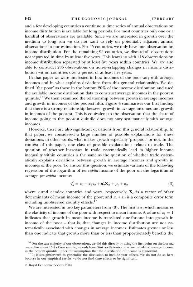
In that paper we were interested in how incomes of the poor vary with averageincomes and in what explains deviations from this general relationship. We de-fined ‘the poor’ as those in the bottom 20% of the income distribution and usedthe available income distribution data to construct average incomes in the poorestquintile.16 We then examined the relationship between growth in average incomesand growth in incomes of the poorest fifth. Figure 4 summarises our first findingthat there is a strong relationship between growth in average incomes and growthin incomes of the poorest. This is equivalent to the observation that the share ofincome going to the poorest quintile does not vary systematically with averageincomes.

However, there are also significant deviations from this general relationship. Inthat paper, we considered a large number of possible explanations for thesedeviations, in other words, what makes growth especially ‘pro-poor’ or not. In thecontext of this paper, one class of possible explanations relates to trade. Thequestion of whether increases in trade systematically lead to higher incomeinequality within countries is the same as the question of whether trade system-atically explains deviations between growth in average incomes and growth inincomes of the poor. To answer this question, we estimate variants of the followingregression of the logarithm of per capita income of the poor on the logarithm ofaverage per capita income:

yPct ¼ a0 þ a1yct þ a0

2Xct þ lc þ ect ð3Þ

where c and t index countries and years, respectively; Xct is a vector of otherdeterminants of mean income of the poor; and lc + ect is a composite error termincluding unobserved country effects.17

We are interested in two key parameters from (3). The first is a1 which measuresthe elasticity of income of the poor with respect to mean income. A value of a1 ¼ 1indicates that growth in mean income is translated one-for-one into growth inincome of the poor – that is, that changes in income distribution are not sys-tematically associated with changes in average incomes. Estimates greater or lessthan one indicate that growth more than or less than proportionately benefits the

16 For the vast majority of our observations, we did this directly by using the first point on the Lorenzcurve. For about 15% of our sample, we only have Gini coefficients and so we calculated average incomein the bottom quintile under the assumption that the distribution of income is lognormal.

17 It is straightforward to generalise the discussion to include year effects. We do not do so herebecause in our empirical results we do not find time effects to be significant.



poor, i.e. that growth systematically leads to decreases or increases in the incomeshare of the poorest quintile. The second parameter of interest is a2 whichmeasures the impact of other determinants of income of the poor over and abovetheir impact on mean income, i.e. the effects of these variables on the income share ofthe poorest quintile. In particular, we can use this regression framework toexamine systematically whether increases in trade volumes (or any other variable)are systematically associated with changes in the income share of the poorestquintile.

Estimating (3) poses a variety of econometric difficulties that we address indetail in our other paper. Here we briefly note that we estimate this equation usinga system generalised method of moments estimator which optimally combinesinformation in the levels of the data with the within-country variation in the data.As discussed in the other paper, this strategy allows us to address, as best we knowhow, problems of measurement error in the income distribution data (and othervariables), possible omitted variables, and the possibility of reverse causation fromincome distribution to average incomes.

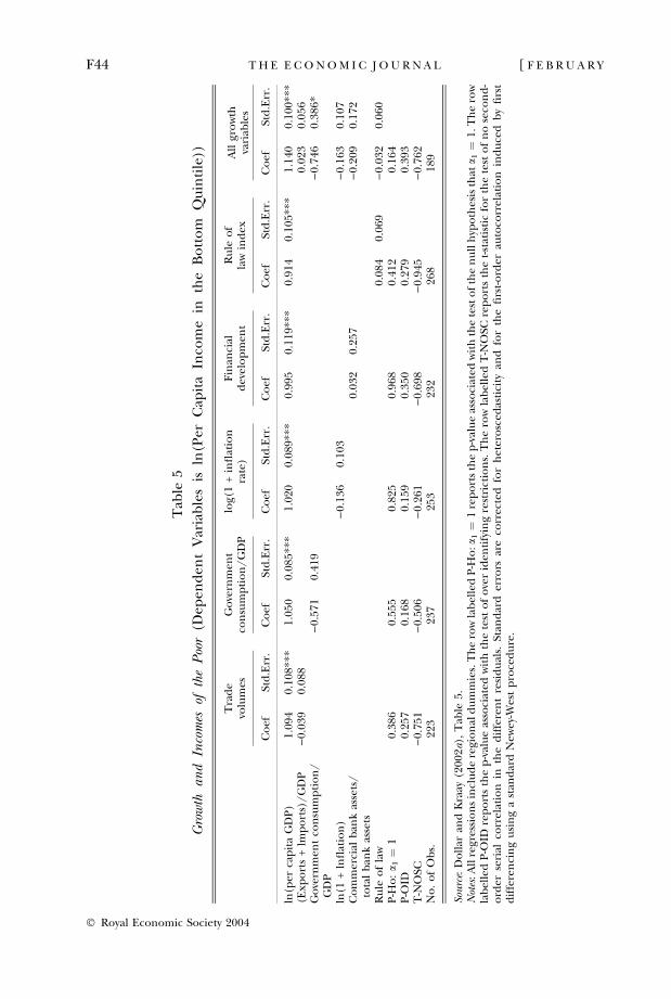
Table 5 shows a typical set of results from that paper, regressing average in-comes of the poorest quintile on average incomes and several additional controlvariables that have been identified as important for growth in the largerempirical growth literature. We typically find a point estimate of a1 which isslightly larger than, but not statistically significantly different from, 1, indicatingthat incomes in the bottom quintile on average rise one-for-one with averageincomes (alternatively, that changes in income distribution are not significantlyassociated with changes in average incomes). In addition, we rarely find that anyof the additional control variables enter significantly, indicating that these vari-ables have no systematic effect on income distribution. The only exception isgovernment consumption, which at times enters significantly. Neither of thesetwo results should be all that surprising. Various authors, including Chen andRavallion (1997) and Deininger and Squire (1996) have documented the strikingabsence of any correlation between (changes in) income and (changes in)inequality, albeit with smaller samples and different econometric techniques.Our lack of systematic significant effects of policies and institutions on inequalitymirrors the dearth of similar robust results in the small empirical literature ondeterminants of income inequality.

For the purposes of this paper, the most interesting results are those relating totrade volumes. Our results indicate that there is no significant correlation betweenchanges in inequality and changes in trade volumes, controlling for changes inaverage incomes (first column of Table 5). This can be seen quite clearly inFigure 5, which reports the simple correlation between changes in trade volumesand changes in inequality as measured by the Gini coefficient (in the top panel)and the logarithm of the first quintile share (in the bottom panel). In Dollar andKraay (2002a) we also subject this basic result to a wide variety of robustness checksand also consider several other measures of international economic integration.Our conclusion is that there simply is no evidence that countries that trade more(or are more integrated along other dimensions) on average have rising incomeinequality. No doubt there are distributional conflicts over trade policy and we do



Tab

le5

Gro

wth

and

Inco

mes

ofth

eP

oor

(Dep

end

ent

Var

iab

les

isln

(Per

Cap

ita

Inco

me

inth

eB

ott

om

Qu

inti

le))

Tra

de

volu

mes

Go

vern

men

tco

nsu

mp

tio

n/

GD

Plo

g(1

+in

flat

ion

rate

)F

inan

cial

dev

elo

pm

ent

Ru

leo

fla

win

dex

All

gro

wth

vari

able

s

Co

efSt

d.E

rr.

Co

efSt

d.E

rr.

Co

efSt

d.E

rr.

Co

efSt

d.E

rr.

Co

efSt

d.E

rr.

Co

efSt

d.E

rr.

ln(p

erca

pit

aG

DP

)1.

094

0.10

8***

1.05

00.

085*

**1.

020

0.08

9***

0.99

50.

119*

**0.

914

0.10

5***

1.14

00.

100*

**(E

xpo

rts

+lm

po

rts)

/G

DP

)0.

039

0.08

80.

023

0.05

6G

ove

rnm

ent

con

sum

pti

on

/G

DP

)0.

571

0.41

9)

0.74

60.

386*

ln(1

+ln

flat

ion

))

0.13

60.

103

)0.

163

0.10

7C

om

mer

cial

ban

kas

sets

/to

tal

ban

kas

sets

0.03

20.

257

)0.

209

0.17

2

Ru

leo

fla

w0.

084

0.06

9)

0.03

20.

060

P-H

o:a 1

¼1

0.38

60.

555

0.82

50.

968

0.41

20.

164

P-O

ID0.

257

0.16

80.

159

0.35

00.

279

0.39

3T

-NO

SC)

0.75

1)

0.50

6)

0.26

1)

0.69

8)

0.94

5)

0.76

2N

o.

of

Ob

s.22

323

725

323

226

818

9

Sou

rce:

Do

llar

and

Kra

ay(2

002a

),T

able

5.N

otes

:All

regr

essi

on

sin

clu

de

regi

on

ald

um

mie

s.T

he

row

lab

elle

dP

-Ho

:a1¼

1re

po

rts

the

p-v

alu

eas

soci

ated

wit

hth

ete

sto

fth

en

ull

hyp

oth

esis

that

a 1¼

1.T

he

row

lab

elle

dP

-OID

rep

ort

sth

ep

-val

ue

asso

ciat

edw

ith

the

test

of

ove

rid

enti

fyin

gre

stri

ctio

ns.

Th

ero

wla

bel

led

T-N

OSC

rep

ort

sth

et-

stat

isti

cfo

rth

ete

sto

fn

ose

con

d-

ord

erse

rial

corr

elat

ion

inth

ed

iffe

ren

tre

sid

ual

s.St

and

ard

erro

rsar

eco

rrec

ted

for

het

ero

sced

asti

city

and

for

the

firs

t-o

rder

auto

corr

elat

ion

ind

uce

db

yfi

rst

dif

fere

nci

ng

usi

ng

ast

and

ard

New

ey-W

est

pro

ced

ure

.



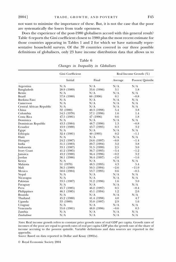
not want to minimise the importance of these. But, it is not the case that the poorare systematically the losers from trade openness.

Does the experience of the post-1980 globalisers accord with this general result?Table 6 reports the Gini coefficient closest to 1980 plus the most recent estimate forthose countries appearing in Tables 1 and 2 for which we have nationally repre-sentative household surveys. Of the 39 countries covered in our three possibledefinitions of globalisers, only 23 have income distribution data that allows us to

Table 6

Changes in Inequality in Globalisers

Gini Coefficient Real Income Growth (%)

Initial Final Average Poorest Quintile

Argentina N/A N/A N/A N/ABangladesh 28.9 (1989) 33.6 (1996) 3.1 1.8Benin N/A N/A N/A N/ABrazil 57.8 (1980) 60 (1996) 0.1 )0.8Burkina Faso N/A N/A N/A N/ACameroon N/A N/A N/A N/ACentral African Republic N/A N/A N/A N/AChina 32 (1980) 40.3 (1998) 5.4 3.8Colombia 54.5 (1978) 57.1 (1996) 1.6 1.4Costa Rica 47.5 (1981) 47 (1996) 0.6 1.8Dominica N/A N/A N/A N/ADominican Republic 43.3 (1984) 48.7 (1996) 1.3 )0.8Ecuador 43.9 (1988) 43.7 (1995) 0.3 3.2Egypt N/A N/A N/A N/AEthiopia 32.4 (1981) 40 (1995) 0.2 )1.1Haiti N/A N/A N/A N/AHungary 24.2 (1987) 24.6 (1997) )0.8 )1.4India 31.5 (1983) 29.7 (1994) 3.2 3.8Indonesia 33.1 (1987) 31.5 (1999) 2.5 3.0Ivory Coast 41.2 (1985) 36.7 (1995) )3.4 )1.2Jamaica 43.2 (1988) 36.4 (1996) )0.2 3.2Jordan 36.1 (1986) 36.4 (1997) )2.0 )1.6Kenya N/A N/A N/A N/AMalaysia 51 (1979) 48.5 (1995) 4.3 5.4Mali 36.5 (1989) 50.5 (1994) )2.6 )11.0Mexico 50.6 (1984) 53.7 (1995) 0.6 )0.5Nepal N/A N/A N/A N/ANicaragua N/A N/A N/A N/APakistan 33.5 (1987) 31.2 (1996) 1.6 3.0Paraguay N/A N/A N/A N/APeru 45.7 (1985) 46.2 (1997) 0.5 )0.4Philippines 46.1 (1985) 45.1 (1994) 1.2 2.6Rwanda N/A N/A N/A N/AThailand 45.2 (1980) 41.4 (1998) 4.0 4.7Uganda 33 (1989) 35.8 (1997) 2.9 1.6Uruguay N/A N/A N/A N/AVenezuela 55.6 (1981) 48.8 (1996) )0.6 0.5Zambia N/A N/A N/A N/AZimbabwe N/A N/A N/A N/A

Notes: Real income growth refers to constant price growth rates of real GDP per capita. Growth rates ofincomes of the poor are equal to growth rates of real per capita GDP plus the growth rate of the share ofincome accruing to the poorest quintile. Variable definitions and data sources are reported in theappendix.Source: Based on data reported in Dollar and Kraay (2002a).



make comparisons of the 1990s relative to the 1980s. In almost exactly half of thesecountries (11 out of 23), income inequality has fallen. So, there are liberalisingeconomies that have had increases in household income inequality over the past20 years, most notably China. But it is not true in general that the liberalisingeconomies have had increases in inequality. Costa Rica’s and Ecuador’s incomedistributions have been quite stable and inequality has declined in countries suchas India, Malaysia, the Philippines and Thailand. Table 6 also shows the averageper capita GDP growth rate over the whole period from the earliest Gini to the latestand the growth rate of income of the bottom 20% of the income distribution.

We want to make three points from this Table. First, because changes ininequality mostly have been small, growth rates of income of the poor are similarto growth rates of per capita GDP. Income of the poor has been rising at more than3% per year in China, India, Malaysia and Thailand – all countries in whichthe growth rate of per capita GDP over the whole period has been strong. Income ofthe poor has declined in Brazil, Mexico and the Ivory Coast, countries in whichthe growth rate of per capita GDP averaged less than 1% over the whole period.Now, we emphasised above that growth rates for almost all of the globalisersaccelerated between the 1980s and 1990s. So, if we divide this period by decade wewould find in countries such as Mexico that income of the poor declined sharply inthe recession years of the 1980s and then increased in the good-growth years of the1990s. The income of the poor tends to be pretty closely tied to the overall state ofthe economy.

But a second interesting fact in the Table is that there are a couple of globalisersthat have had large declines in inequality, with the result that income of the poorrose quite a bit more rapidly than mean income. Malaysia and Thailand are thebest examples. (Note, ironically, that despite the financial crisis that started in1997, Thailand had one of the fastest growth rates of income of the poor: 4.7% peryear from 1980 to 1998.) Obviously, the combination of rapid growth and higherincome share for the poor is best for poverty reduction. However, we have to stressthat it is difficult to discern any common feature or pattern to the cases where weobserve this in the data.

The third point that we want to make from the Table is that growth rate ofincome of the poor has significantly lagged the growth rate of per capita GDP inChina, a transition economy in which there has been a large increase in inequality.But despite the change in inequality, the growth rate of income of the poor inChina has still been high (3.8% per year) and there has been a dramatic decline inabsolute poverty there. While the large increase in inequality is disconcerting, itwould be misleading to attribute it entirely to greater openness as the transitioncountries have undergone dramatic changes in their entire economic systems overthe past two decades. But, whatever its source, there are likely to be measures thatcan be taken to reverse the trend. Our own reading of history and data is thatmeasures that can successfully raise income share of the poor without harminggrowth are likely to be country-specific. In China, for example, poor transport linksbetween interior regions and the coast and restrictions on inter-provincialmigration are factors that probably contribute to growing inequality and areamenable to policy interventions.



In summary, we have found no evidence of a systematic effect of trade volumeson income inequality. Combining this observation with the results on the growthbenefits of greater trade, we conclude that the balance of the evidence suggeststhat, on average, greater globalisation is a force for poverty reduction.

3. Conclusion

We have identified a group of developing countries that have had large cuts intariffs and large increases in actual trade volumes since 1980. Since China, Indiaand several other large countries are part of this group, well over half of thepopulation of the developing world lives in these globalising economies. The post-1980 globalisers are different from the rest of the developing world in terms of theextent of tariff cutting (22 point reduction compared to 10 points) and in terms ofthe increase in trade volume over the past 20 years (an increase from 16% to 32%of GDP, versus a decline from 60% of GDP to 49% of GDP). While rich countrygrowth rates have slowed down over the past several decades, the growth rates ofthe globalisers have shown exactly the opposite pattern, accelerating from the1970s to the 1980s to the 1990s. The rest of the developing world, on the otherhand, has followed the same pattern as the rich countries: growth deceleratingfrom the 1970s to the 1980s to the 1990s. In the 1990s the globalising developingcountries grew at 5.0% per capita; rich countries at 2.2% and non-globalisingdeveloping countries at only 1.4%. Thus, the globalisers are catching up with richcountries while the non-globalisers fall further and further behind.

We also looked at how general these patterns are, through cross-countryregressions. We focused on within country variation and showed that changes intrade volumes have a strong positive relationship to changes in growth rates.Furthermore, there is no systematic relationship between changes in trade vol-umes and changes in household income inequality. The increase in growth ratesthat accompanies expanded trade therefore on average translates into propor-tionate increases in income of the poor. Thus, absolute poverty in the globalisingdeveloping economies has fallen sharply in the past 20 years. The evidence fromindividual cases and from cross-country analysis supports the view that opentrade regimes lead to faster growth and poverty reduction in poor countries.

The World Bank

AppendixVariable Definitions and Data Sources

Variable Source Comments

(Exports + lmports)/GDP

World Bank Data Numerator and denominator arein constant local currency units.

Real GDP per capita Summers and HestonPenn World Tables,World Bank Data

Constant 1985 US dollars. Extendedto 1998 using constant price localcurrency growth rates. Extendedcross-sectionally as describedin Kraay et al. (2000).



Appendix (Continued)

Variable Source Comments

Population World Bank Data Mid-Year populationTariffs Sources: WTO, IDB database

and Trade Policy Review –Country Report, Various issues,1990–2000; UNCTAD, Handbookof Trade Control Measures of DevelopingCountries – Supplement, 1987and Directory of Import Regimes, 1994;World Bank, Trade Policy Reform

All tariff rates are basedon unweighted averagesfor all goods in ad valoremrates, or applied rates,or MFN rates whicheverdata are available in alonger period.

First quintile share UN-WIDER (2000), Deininger andSquire (1996), Ravallionand Chen (2000), Lundbergand Squire (2000)

Combination of datafrom different sourcesdescribed in more detail inDollar and Kraay (2002a)

Gini coefficient UN-WIDER (2000), Deiningerand Squire (1996), Ravallionand Chen (2000), Lundbergand Squire (2000)

Combination of data fromdifferent sources describedin more detail in Dollarand Kraay (2002a)

Contract-intensivemoney

IMF International Financial Statistics 1-currency in circulation/M2,as described in Clague et al. (1999).

Governmentconsumption/GDP

World Bank Data Numerator and denominatorare in current local currency units.

ln(1 + inflation) World Bank Data Inflation is CPI-based where available,otherwise use growth of GDP deflator.

References

Ades, A. and Glaeser, E. (1999). ‘Evidence on growth, increasing returns, and the extent of the market’,Quarterly Journal of Economics, vol. 114(3), pp. 1025–46.

Arellano, M. and Bover, O. (1995). ‘Another look at the instrumental-variable estimation of error-components models’, Journal of Econometrics, vol. 68, pp. 29–52.

Blundell, R. and Bond, S. (1998). ‘Initial conditions and moment restrictions in dynamic panel datamodels’, Journal of Econometrics, vol. 87, pp. 115–43.

Caselli, F., Esquivel, G. and Lefort, F. (1996). ‘Reopening the convergence debate: a new look at cross-country growth empirics’, Journal of Economic Growth, vol. 1, pp. 363–89.

Chen, S. and Ravallion, M. (1997). ‘What can new survey data tell us about recent changes in distri-bution and poverty?’, The World Bank Economic Review, vol. 11(2), pp. 357–82.

Clague, C., Keefer, P., Knack, S. and Olson, M. (1999). ‘Contract-intensive money: contract enforce-ment, property rights, and economic performance’, Journal of Economic Growth, vol. 4, pp. 185–211.

Deininger, K. and Squire, L. (1996). ‘A new data set measuring income inequality’, The World BankEconomic Review, vol. 10(3), pp. 565–91.

Desai, P. (ed.) (1997). Going Global: Transition from Plan to Market in the World Economy, Cambridge MA:MIT Press.

Dollar, D. (1992). ‘Outward-oriented developing countries really do grow more rapidly: evidence from95 LDCs, 1976–85’, Economic Development and Cultural Change, vol. 40(3), (April), pp. 523–44.

Dollar, D. and Kraay, A. (2002a). ‘Growth is good for the poor’, Journal of Economic Growth, vol. 7,pp. 195–225.

Dollar, D. and Kraay, A. (2002b). ‘Institutions, trade, and growth’, Journal of Monetary Economics, vol. 50,pp. 133–62.

Dollar, D. and Kraay, A. (2003). ‘Institutions, trade, and growth: revisiting the evidence’, World BankPolicy Research Department Working Paper No. 3004.

Edwards, S. (1992). ‘Trade orientation, distortions, and growth in developing countries’, Journal ofDevelopment Economics, vol. 39(1), pp. 31–57.

Frankel, J.A. and Romer, D. (1999). ‘Does trade cause growth?’, American Economic Review, vol. 89 (June),pp. 379–99.

Kraay, A., Loayza, S., Serven, J. and Ventura, (2000). ‘Country portfolios’, NBER Working Paper 7795.Levine, R. and Renelt, D. (1992). ‘A sensitivity analysis of cross-country growth regressions’, American

Economic Review, vol. 82 (4) (September), pp. 942–63.



Lundberg, M. and Squire, L. (2000). ‘The simultaneous evolution of growth and inequality’, mimeo,The World Bank.

Ravaillion, M. and Chen, S. (2000). ‘How did the world’s poorest fare in the 1990s’, World Bank PolicyResearch Department Working Paper 2409.

Rodriguez, F. and Rodrik, D. (2000). ‘Trade policy and economic growth: a skeptic’s guide to the cross-national evidence’, in (B. Bernanke and K. Rogoff, eds.), Macroeconomics Annual 2000, CambridgeMA: MIT Press for NBER.

Rodrik, D. (1999). Making Openness Work: The New Global Economy and the Developing Countries,Washington, DC: Overseas Development Council.

Rodrik, D. (2000). ‘Trade policy reform as institutional reform’, mimeo, Harvard University.Sachs, J.D. and Warner, A. (1995). ‘Economic reform and the process of global integration’, Brookings

Papers on Economic Activity, no. 1, pp. 1–118.Srinivasan, T.N., and Bhagwati, J. (1999). ‘Outward-orientation and development: are revisionists

right?’, mimeo, Yale University.UN-WIDER (2000). ‘World income inequality database’, available online at www.wider.uni.edu/wiid/

wiid.htm.



Documents

Inequality