Introduc„on to Dynamic Programming and Applica„on from Erich … · Applica„on from Erich French (2005) ScPo Graduate Labor February 23, 2017 1/79. Table of contents Dynamic

Introduc�on to Dynamic Programming andApplica�on from Erich French (2005)ScPo Graduate Labor

February 23, 2017

1 / 79

Table of contents

Dynamic ProgrammingDynamic Programming: Piece of CakeDynamic Programming TheoryStochas�c Dynamic Programming

Applica�on to Labor Supply: French (2005)ModelEs�ma�onResults

2 / 79



3 / 79

Introduc�on

• This lecture will introduce you to a powerful technique calleddynamic programming (DP).

• This set of slides is very similar to the one from your grad macrocourse. (same teacher.)• We will repeat much of that material today.• Then we will talk about a paper that uses DP to solve a dynamiclifecycle model.

4 / 79

References

• Before we start, some useful references on DP:1 Adda and Cooper (2003): Dynamic Economics.2 Ljungqvist and Sargent (2012) (LS): Recursive MacroeconomicTheory.3 Lucas and Stokey (1989): Recursive Methods in EconomicsDynamics.

• They are ordered in increasing level of mathema�cal rigor. Addaand Cooper is a good overview, LS is rather short.

5 / 79

Cake Ea�ng• You are given a cake of size W1 and need to decide how much ofit to consume in each period t = 1, 2, 3, . . .• Cake consump�on valued as u(c), u is concave, increasing,differen�able and limc→0 u′(c) = ∞.• Life�me u�lity is

U =T

∑t=1

βt−1u(ct), β ∈ [0, 1] (1)• Let’s assume the cake does not depreciate/perish, s.t. the law ofmo�on of cake is

Wt+1 = Wt − ct, t = 1, 2, ..., T (2)i.e. cake in t + 1 is this cake in t minus whatever you have of it in t.

• How to decide on the op�mal consump�on sequence {ct}Tt=1?

6 / 79

A sequen�al Problem• This problem can be wri�en as

v (W1) = max{Wt+1,ct}T

t=1

T

∑t=1

βt−1u(ct) (3)s.t.

Wt+1 = Wt − ct

ct, Wt+1 ≥ 0 and W1 given.• No�ce that the law of mo�on (2) implies that

W1 = W2 + c1

= (W3 + c2) + c1

= . . .

= WT+1 +T

∑t=1

ct (4)7 / 79

Solving the sequen�al Problem• Formulate and solve the Lagrangian for (3) with (4):

L =T

∑t=1

βt−1u(ct) + λ

[W1 −WT+1 −

T

∑t=1

ct

]+ φ [WT+1]

• First order condi�ons:∂L∂ct

= 0 =⇒ βt−1u′(ct) = λ ∀t (5)∂L

∂WT+1= 0 =⇒ λ = φ (6)

• φ is lagrange mul�plier on non-nega�vity constraint for WT+1.• we ignore the constraint ct ≥ 0 by the Inada assump�on.

8 / 79

Solving the sequen�al Problem• Formulate and solve the Lagrangian for (3) with (4):

L =T

∑t=1

βt−1u(ct) + λ

[W1 −WT+1 −

T

∑t=1

ct

]+ φ [WT+1]

• First order condi�ons:∂L∂ct

= 0 =⇒ βt−1u′(ct) = λ ∀t (5)∂L

∂WT+1= 0 =⇒ λ = φ (6)

• φ is lagrange mul�plier on non-nega�vity constraint for WT+1.• we ignore the constraint ct ≥ 0 by the Inada assump�on.8 / 79

Interpre�ng the sequen�al solu�on• From (5) we know that βt−1u′(ct) = λ holds in each t.• Therefore

βt−1u′(ct) = λ

= β(t+1)−1u′(ct+t)

i.e. we get the Euler Equa�onu′(ct) = βu′(ct+1) (7)

• along an op�mal sequence {c∗t }Tt=1, each adjacent period

t, t + 1 must sa�sfy (7).• If (7) holds, one cannot increase u�lity by moving some ct to

ct+1.• What about devia�on from {c∗t }T

t=1 between t and t + 2?9 / 79

Is the Euler Equa�on enough?• Is the Euler Equa�on sufficient for op�mality?

• No! We could sa�sfy (7), but have WT > cT, i.e. there is somecake le�.• What does this remind you of?• Discuss how this relates to the value of mul�pliers λ, φ.• Solu�on is given by ini�al condi�on (W1), terminal condi�on

WT+1 = 0 and path in EE.• Call this solu�on the value func�on

v (W1)

• v (W1) is the maximal u�lity flow over T periods given ini�alcake W1.

10 / 79

Is the Euler Equa�on enough?• Is the Euler Equa�on sufficient for op�mality?• No! We could sa�sfy (7), but have WT > cT, i.e. there is somecake le�.• What does this remind you of?• Discuss how this relates to the value of mul�pliers λ, φ.• Solu�on is given by ini�al condi�on (W1), terminal condi�on

WT+1 = 0 and path in EE.• Call this solu�on the value func�on

v (W1)

• v (W1) is the maximal u�lity flow over T periods given ini�alcake W1.10 / 79

The Dynamic Programming approach with T = ∞

• Let’s consider the case T = ∞.• In other words

max{Wt+1,ct}∞

t=1

∞

∑t=1

βt−1u(ct) (8)s.t.

Wt+1 = Wt − ct (9)• Under some condi�ons, this can be wri�en as

v(Wt) = maxct∈[0,Wt]

u (ct) + βv(Wt − ct) (10)• Some Defini�ons:

• Call W the state variable,• and c the control variable.• (9) is the law of mo�on or transi�on equa�on.

11 / 79

The Dynamic Programming approach with T = ∞

• Note that t is irrelevant in (10). Only W ma�ers.• Subs�tu�ng c = W−W′, where x′ is next period’s value of x

v(W) = maxW′∈[0,W]

u(W−W′

)+ βv(W′) (11)

• This is the Bellman Equa�on a�er Richard Bellman.• It is a func�onal equa�on (v is on both sides!).• Our problem has changed from finding {Wt+1, ct}∞

t=1 to findingthe func�on v.This is called a fixed point problem:Find a func�on v such that plugging in W on the RHS and doing themaximiza�on, we end up with the same v on the LHS.

12 / 79

Value Func�on and Policy Func�on• Great! We have reduced an infinite-length sequen�al problemto a one-dimensional maximiza�on problem.• But we have to find 2(!) unknown func�ons! Why two?• The maximizer of the RHS of (11) is the policy func�on,

g (W) = c∗.• This func�on gives the op�mal value of the control variable,given the state.• It sa�sfies

v (W) = u (g (W)) + βv (g (W)) (12)(you can see that the max operator vanished, because g(W) isthe op�mal choice)

• In prac�ce, finding value and policy func�on is the oneopera�on.13 / 79

Using Dynamic Programming to solve the Cake problem• Let’s pretend that we knew v for now:

v(W) = maxW′∈[0,W]

u(W−W′

)+ βv(W′)

• Assuming v is differen�able, the FOC wrt W′

u′(c) = βv′(W′) (13)

• Taking the par�al deriva�ve w.r.t. the state W, we get theenvelope condi�on

v′(W) = u′(c) (14)• This needs to hold in each period. Therefore

v′(W′) = u′(c′) (15)

14 / 79

Using Dynamic Programming to solve the Cake problem

• Combining (13) with (15)u′(c) (13)

= βv′(W′)

(15)= βu′(c′)

we obtain the usual euler equa�on.• Any solu�on vwill sa�sfy this necessary condi�on, as in thesequen�al case.

• So far, so good. But we s�ll don’t know v!

15 / 79

Using Dynamic Programming to solve the Cake problem

• Combining (13) with (15)u′(c) (13)

= βv′(W′)

(15)= βu′(c′)

we obtain the usual euler equa�on.• Any solu�on vwill sa�sfy this necessary condi�on, as in thesequen�al case.• So far, so good. But we s�ll don’t know v!

15 / 79

Finding v

• Finding the Bellman equa�on v and associated policy func�on gis not easy.• In general, it is impossible to find an analy�c expression, i.e. todo it by hand.• Most of �mes you will use a computer to solve for it.• preview: The ra�onale for why we can find it has to do with thefixed point nature of the problem. We will see that under somecondi�ons we can always find that fixed point.• We will look at a par�cular example now, that we can solve byhand.

16 / 79

Finding v: an example with closed form solu�on• Let’s assume that u(c) = ln c in (11).• Also, let’s conjecture that the value func�on has the form

v(W) = A + B ln W (16)• We have to find A, B such that (16) sa�sfies (11).• Plug into (11):

A + B ln W = maxW′

ln(W−W′

)+ β

(A + B ln W′

) (17)

• FOC wrt W′:1

W−W′=

βBW′

W′ = βB(W−W′)

W′ =βB

1 + βBW

≡ g(W)

17 / 79

Finding v: an example with closed form solu�on• Let’s assume that u(c) = ln c in (11).• Also, let’s conjecture that the value func�on has the form

v(W) = A + B ln W (16)• We have to find A, B such that (16) sa�sfies (11).• Plug into (11):

A + B ln W = maxW′

ln(W−W′

)+ β

(A + B ln W′

) (17)• FOC wrt W′:

1W−W′

=βBW′

W′ = βB(W−W′)

W′ =βB

1 + βBW

≡ g(W)

17 / 79

Finding v: an example with closed form solu�on• Let’s use this policy func�on in (17):

v(W) = ln (W− g(W)) + β (A + B ln g(W))

= lnW

1 + βB+ β

(A + B ln

[βB

1 + βBW])

• Now we collect all terms ln W on the RHS, and put all else intothe constant A:v(W) = A + ln W + βB ln W

= A + (1 + βB) ln W

• We conjectured that v(W) = A + B ln W. HenceB = (1 + βB)

B =1

1− β

• Policy func�on: g(W) = βW18 / 79

The Guess-and-Verify method

• Note that we guessed a func�onal form for v.• And then we verified that it consitutues a solu�on to thefunc�onal equa�on.• This method (guess and verify) would in principle always work,but it’s not very prac�cal.

19 / 79

Solving the Cake problem with T < ∞

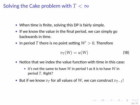
• When �me is finite, solving this DP is fairly simple.• If we know the value in the final period, we can simply gobackwards in �me.• In period T there is no point se�ng W′ > 0. Therefore

vT(W) = u(W) (18)• No�ce that we index the value func�on with �me in this case:

• it’s not the same to have W in period 1 as it is to have W inperiod T. Right?• But if we know vT for all values of W, we can construct vT−1!

20 / 79

Backward Induc�on and the Cake Problem• We know that

vT−1 (WT−1) = maxWT∈[0,WT−1]

u (WT−1 −WT) + βvT (WT)

= maxWT∈[0,WT−1]

u (WT−1 −WT) + βu (WT)

= maxWT∈[0,WT−1]

ln (WT−1 −WT) + β ln WT

• FOC wrt WT:1

WT−1 −WT=

β

WT

WT =β

1 + βWT−1

• Thus the value func�on in T− 1 isvT−1 (WT−1) = ln

(WT−1

β

)+ β ln

(β

1 + βWT−1

)21 / 79

Backward Induc�on and the Cake Problem• Correspondingly, in T− 2:

vT−2 (WT−2) = maxWT−1∈[0,WT−2]

u (WT−2 −WT−1) + βvT−1 (WT−1)

= maxWT−1∈[0,WT−2]

u (WT−2 −WT−1)

+ β

[ln(

WT−1

β

)+ β ln

(β

1 + βWT−1

)]• FOC wrt WT−2.• and so on un�l t = 1.• Again, without log u�lity, this quickly get intractable. But yourcomputer would proceed in the same backwards itera�ngfashion.• No�ce that with T finite, there is no fixed point problem if we dobackwards induc�on.

22 / 79

Dynamic Programming Theory

• Let’s go back to the infinite horizon problem.• Let’s define a general DP as follows.• Payoffs over �me are

U =∞

∑t=1

βtu (st, ct)

where β < 1 is a discount factor, st is the state, ct is the control.• The state (vector) evolves as st+1 = h(st, ct).• All past decisions are contained in st.

23 / 79

DP Theory: more assump�ons• Let ct ∈ C(st), st ∈ S and assume u is bounded in(c, s) ∈ C× S.

• Sta�onarity: neither payoff u nor transi�on h depend on �me.• Modify u to u s.t. in terms of s′ (as in cake: c = W−W′):

v(s) = maxs′∈Γ(s)

u(s, s′) + βv(s′) (19)• Γ(s) is the constraint set (or feasible set) for s′ when the currentstate is s:

• before that was Γ(W) = [0, W]

• We will work towards one possible set of sufficient condi�onsfor the existence to the func�onal equa�on. Please consultStokey and Lucas for greater detail.

24 / 79

Proof of Existence

TheoremAssume that u(s, s′) is real-valued, con�nuous, and bounded, thatβ ∈ (0, 1), and that the constraint set Γ(s) is nonempty, compact,and con�nuous. Then there exists a unique func�on v(s) that solves(19).

Proof.Stokey and Lucas (1989, theoreom 4.6).

25 / 79

The Bellman Operator T(W)

• Define an operator Ton func�on W as T(W):

T(W)(s) = maxs′∈Γ(s)

u(s, s′) + βW(s′) (20)• The Bellman operator takes a guess of current value func�on W,performs the maximiza�on, and returns the next value func�on.• Any v(s) = T(v)(s) is a solu�on to (19).• So we need to find a fixed point of T(W).• This argument proceeds by showing that T(W) is a contrac�on.• Info: This relies on the Banach (or contrac�on) mappingtheorem.

• There are two sufficiency condi�ons we can check:Monotonicity, and Discoun�ng.

26 / 79

The Blackwell (1965) sufficiency condi�ons: Monotonicity• Need to check Monotonicity and Discoun�ng of the operator

T(W).• Monotonicitymeans that

W(s) ≥ Q(s) =⇒ T(W)(s) ≥ T(Q)(s), ∀s

• Let φQ(s) be the policy func�on ofQ(s) = max

s′∈Γ(s)u(s, s′) + βQ(s′)

and assume W(s) ≥ Q(s). ThenT(W)(s) = max

s′∈Γ(s)u(s, s′) + βW(s′) ≥ u(s, φQ(s)) + βW(φQ(s))

≥ u(s, φQ(s)) + βQ(φQ(s)) ≡ T(Q)(s)

Show example with W(s) = log(s2), Q(s) = log(s), s > 0

27 / 79

The Blackwell (1965) sufficiency condi�ons: Discoun�ng• Adding constant a to W leads T(W) to increase less than a.• In other words

T(W + a)(s) ≤ T(W)(s) + βa, β ∈ [0, 1)

• discoun�ng because β < 1.• To verify on the Bellman operator:

T(W+ a)(s) = maxs′∈Γ(s)

u(s, s′)+ β[W(s′) + a

]= T(W)(s)+ βa

• Intui�on: the discoun�ng property is key for a contrac�on.• In successive itera�ons on T(W) we add only a frac�on β of W.

28 / 79

Contrac�on Mapping Theorem (CMT)• The CMT tells us that for a func�on of type T(·)

1 There is a unique fixed point. (from previous Stokey-Lucas proof.)2 This fixed point can be reached by itera�ng on T in (20) using an

arbitrary star�ng point.

• Very useful to find a solu�on to (19):1 Start with an ini�al guess V0(s).2 Apply the Bellman operator to get V1 = T(V0)

1 if V1(s) = V0(s) we have a solu�on, done.2 if not, con�nue:3 Apply the Bellman operator to get V2 = T(V1)4 etc un�l T(V) = V.

• Again: if T(V) is a contrac�on, this will converge.• This technique is called value func�on itera�on.

29 / 79

Value Func�on inherits Proper�es of u

TheoremAssume u(s, s′) is real-values, con�nuous, concave and bounded,0 < β < 1, that S is a convex subset of Rk and that the constraint setΓ(s) is non-empty, compact-valued, convex, and con�nuous. Then theunique solu�on to (19) is strictly concave. Furthermore, the policyφ(s) is a con�nuous, single-valued func�on.

Proof.See theorem 4.8 in Stokey and Lucas (1989).

30 / 79

Value Func�on inherits Proper�es of u

• proof shows that if V is concave, so is T(V).• Given u(s, s′) is concave, let the ini�al guess be

V0(s) = maxs′∈Γ(s)

u(s, s′)

and therefore V0(s) is concave.• Since T preserves concavity, V1 = T(V0) is concave etc.

31 / 79

Stochas�c Dynamic Programming

• There are several ways to include uncertainty into thisframework - here is one:• Let’s assume the existence of a variable ε, represen�ng a shock.• Assump�ons:

1 εt affects the agent’s payoff in period t.2 εt is exogenous: the agent cannot influence it.3 εt depends only on εt−1 (and not on εt−2. although we couldadd εt−1 as a state variable!)4 The distribu�on of ε′|ε is �me-invariant.

• Defined in this way, we call ε a first-order Markov process.

32 / 79

The Markov Property

Defini�onA stochas�c process {xt} is said to have theMarkov property if for allk ≥ 1 and all t,

Pr (xt+1|xt, xt−1, . . . , xt−k) = Pr (xt+1|xt) .

We assume that {εt} has this property, and characterize it by aMarkov Chain.

33 / 79

Markov ChainsDefini�onA �me-invariant n-State Markov Chain consists of:

1 n vectors of size (n, 1): ei, i = 1, . . . , n such that the i-th entry ofei is one and all others zero,

2 one (n, n) transi�on matrix P, giving the probability of movingfrom state i to state j, and3 a vector π0i = Pr (x0 = ei) holding the probability of being instate i at �me 0.• e1 =

[1 0 . . . 0

]′, e2 =

[0 1 . . . 0

]′, . . . are just a way

of saying “x is in state i”.• The elements of P are

Pij = Pr(xt+1 = ej|xt = ei

)34 / 79

Assump�ons on P and π0

1 For i = 1, . . . , n, the matrix P sa�sfiesn

∑j=1

Pij = 1

2 The vector π0 sa�sfiesn

∑i=1

π0i = 1

• In other words, P is a stochas�c matrix, where each row sums toone:• row i has the probabili�es to move to any possible state j. A validprobability distribu�on must sum to one.

• P defines the probabili�es of moving from current state i tofuture state j.• π0 is a valid ini�al probability distribu�on.

35 / 79

Transi�on over two periods

• The probability to move from i to j over two periods is given byP2

ij.• Why:Pr(xt+2 = ej|xt = ei

)=

n

∑h=1

Pr(xt+2 = ej|xt+1 = eh

)Pr (xt+1 = eh|xt+1 = ei) =

n

∑h=1

PihPhj = P(2)ij

• Show 3-State example to illustrate this.

36 / 79

Condi�onal Expecta�on from a Markov Chain• What is expected value of xt+1 given xt = ei?• Simple:

E [xt+1|xt = ei] = values of x× Prob of those values=

n

∑j=1

ej × Pr(xt+1 = ej|ei

)=

[x1 x2 . . . xn

](Pi)

′

where Pi is the i-th row of P, and (Pi)′ is the transpose of thatrow (i.e. a column vector).

• What is the condi�onal expecta�on of a func�on f (x), i.e. whatisE [f (xt+1)|xt = ei]?

37 / 79

Back to Stochas�c DP• With the Markovian setup, we can rewrite (19) as

v(s, ε) = maxs′∈Γ(s,ε)

u(s, s′, ε) + βE[v(s′, ε′)|ε

] (21)TheoremIf u(s, s′, ε) is real-valued, con�nuous, concave, and bounded, ifβ ∈ (0, 1), and constraint set is compact and convex, then

1 there exists a unique value func�on v(s, ε) that solves (21).2 there exists a sta�onary policy func�on φ(s, ε).

Proof.This is a direct applica�on of Blackwell’s sufficiency condi�ons:1 with β < 1 discoun�ng holds for the operator on (21).2 Monotonicity can be established as before.

38 / 79

Op�mality in the Stochas�c DP

• As before, we can derive the first order condi�ons on (21):us′(s, s′, ε) + βE

[Vs′(s′, ε′)|ε

]= 0

• differen�a�ng (21) w.r.t. s to find Vs′(s′, ε′) we findus′(s, s′, ε) + βE

[us′(s′, s′′, ε′)|ε

]= 0

39 / 79

DP Applica�on 1: The Determinis�c Growth Model• We will now solve the determinis�c growth model with dynamicprogramming.• Remember:

V(k) = maxc=f (k)−k′≥0

u(c) + βV(k′) (22)• Assume f (k) = kα, u(c) = ln c.• We will use discrete state DP.We cannot hope to know V at all

k ∈ R+. Therefore we compute V at a finite set of points, calleda grid.• Hence, we must also choose those grid points.

40 / 79

DP Applica�on: Discre�ze state and solu�on space

• There are many ways to approach this problem:V(k) = max

k′∈[0,kα]ln(kα − k′) + βV(k′) (23)

• Probably the easiest goes like this:1 Discre�ze V onto a grid of n points K ≡ {k1, k2, . . . , kn}.2 Discre�ze control k′: change maxk′∈[0,kα ] to maxk′∈K, i.e. choose

k′ from the discrete grid.3 Guess an ini�al func�on V0(k).4 Iterate on (23) un�l d (Vt+1 −Vt) < ε, where d() is a measureof distance, and ε > 0 is a tolerance level chosen by you.

41 / 79



42 / 79

Applica�on to Labor Supply: French (2005)

• How does labor supply relate to the Social Security and Pensionsystems?

• How does health enter this picture?• We need a dynamic model here: you will work differently ifyou expect to get a pension at age 60.

43 / 79

French (2005) Structure

• People in the model can save (not borrow).• There is random income each period.• People probabilis�cally age (i.e. if they don’t die, they get a yearolder)• Health evolves over this lifecycle in a state-dependent fashion.

44 / 79

Policy Simula�ons

• Once es�mated, use the model for policy experiments• Change re�rement age from 62 to 63.• Reduce Social Security (SS) Benefits by 20 %• Eliminate tax wage from SS meanstest.

45 / 79

Model• Choose consump�on and hours Ct, Ht as well as whether toapply for SS, Bt ∈ {0, 1}

• Health status is Mt, which enters u�lity:U(Ct, Ht, Mt)

• There is a bequest func�on b(AT), where At are assets.• Denote st the probability of being alive at t, given alive at t− 1.• Hence, S(j, t) = 1

stΠj

k=tsk is prob of living through j, given aliveat t

• You die for sure in T + 1, hence sT+1 = 0.

46 / 79



47 / 79

Model• At �me t, life�me u�lity is

U(Ct, Ht, Mt)+

Et

[T+1

∑j=t+1

βjS(j− 1, t)(sjU(Cj, Hj, Mj) + (1− sj)b(Aj)

](24)

• Applying for SS sets Bt = 1

• The problem of the consumer is to choose a plan{Cj, Hj, Bj}T+1

t=j that maximizes (24), subject to1 mortality determina�on2 health determina�on3 wage determina�on4 spousal income5 and a budget constraint.

48 / 79

U�lity Func�on

Within period u�lity isU(Ct, Ht, Mt) =

11− ν

(Cγ

t (L−Ht − θPPt − φ1{M = bad})1−γ)1−ν

(25)where1 leisure is L−Ht − θPPt − φ1{M = bad}2 Health is good/bad when M = {0, 1}.3 If par�cipate in labor force, Pt = 1, and pay fixed cost θP

4 Re�rement: set H = 0. Can re-enter labor at any �me.

49 / 79

Role of U�lityThe distribu�on of annual hours of work is clustered

around both 2000 and 0 hours of work, a regularity in thedata that standard u�lity func�ons have a difficult �mereplica�ng. Fixed costs of work are a common way ofexplaining this regularityin the data (Cogan, 1981). Fixedcosts of work generate a reserva�on wage for a givenmarginal u�lity of wealth. Below the reserva�on wage,hours worked is zero. Slightly above the reserva�on wage,hours worked may be large. Individual level labour supplyi shighly responsive aroundthis reserva�on wage levelalthough wage increases above the reserva�on wage resultin a smaller labour supply response.

50 / 79

Bequest, Health and Survival• The bequest func�on is

b(At) = θB(At + K)(1−ν)γ

1− ν

• Survival is a func�on of age and healthst+1 = s(Mt, t + 1)

• Health evolves according to a markov chainπgood,bad,t+1 = Pr(Mt+1 = good|Mt = bad, t + 1)

51 / 79

Wages

• Wages are given byln Wt = α ln Ht + W(Mt, t) + ARt (26)

• W(·) is an age profile, AR an autoregressive component.ARt = ρARt−1 + ηt, η ∼ N(0, σ2

η)

• Spousal income isyst = ys(Wt, t) (27)

52 / 79

Budget constraintThe budget constraint is

At+1 = At + Y(xt, τ) + Bt × sst − Ct ≥ 0 (28)with the func�on Y measuring post tax income, r interest, pbpension, ss social security, and

xt = rAt + WtHt + yst + pbt + εt (29)

• Social Security available only a�er age 62. It lasts �ll death.• Similarly, pension benefits are paid out a�er age 62.

53 / 79

Social Security and Re�ring at 65

• SS benefits depend on Averaged Indexed Monthly Earnings,AIME. This is average earnings in the 35 highest-paying years.

• Incen�ves to start SS at age 65: from 62-65, every early yearreduces benefits by 6.7%. From 65-70, every addi�onal workyear increases benefits only by 3%.• Under 70 year-olds who work while on SS are taxed heavily.Earnings above 6000$ per year are taxed at 50% (plus federal,state and payroll tax).

54 / 79

Pensions

• Pensions are similar. Pension wealth is typically illiquid before acertain age.• Also a func�on of AIME.• Focus on defined benefit pension plans. The pension formula isdefined and known in advance. The pension does not depend onstock market returns, for example.

55 / 79

Model Solu�on• The state vector is Xt = (At, Wt, Bt, Mt, AIMEt)

• Preferences are θ = (γ, ν, θP, θB, φ, L, β)

• The value func�on solvesVt(Xt) = max

Ct,Ht,Bt

{U(Ct, Ht, Mt)

+βst+1 ∑M∈good,bad

∫Vt+1(Xt+1)dF(Wt+1|Mt+1, Wt, t)π(Mt+1|Mt, t)

+β(1− st+1b(At+1))} (30)

• Backward induc�on over grids X and C,H

56 / 79



57 / 79

Es�ma�on: 2 Steps

Es�ma�on proceeds in two steps:1 Es�mate laws of mo�on for exogenous state variables outside ofthe model, and calibrate others to reasonable values.2 Use those processes as given in the model, and find a set ofpreference parameters that generates model output as close aspossible to observed data.

58 / 79

Simulated Method of Moments as Extremum Es�matorDefini�on: Extremum Es�mator

An es�mator θ of dimension p is called and extremum es�ma-tor if there is a scalar objec�ve func�on Qn : Rp 7→ R and aparameter space Θ ⊂ Rp such that

θ = arg maxθ∈Θ

Qn(θ)

• OLS• GMM/SMM• IV• MLE

59 / 79

GMMmoment func�onThe Generalized Method of Moments relies on a set of K momentcondi�ons which provide limited informa�on about a parameter θ,given a set of data wi:

E[g(wi; θ︸︷︷︸p×1

] = 0︸︷︷︸K×1

(31)

This has sample analog:gn(θ) =

1n

n

∑i=1

g(wi; θ) (32)Can we solve (31)?

60 / 79

GMM Es�matorDefini�on: GMM Es�mator

The GMM es�mator θ(W) of θ sa�sfyingE[g(wi; θ︸︷︷︸

p×1

] = 0︸︷︷︸K×1

with θ ∈ ∆ ⊂ Rp is defined asθ(W) = arg min

θ∈∆ngn(θ)

′Wgn(θ) (33)where W is a K× K weigh�ng matrix that may depend on thedata and is symmetric and p.d.

61 / 79

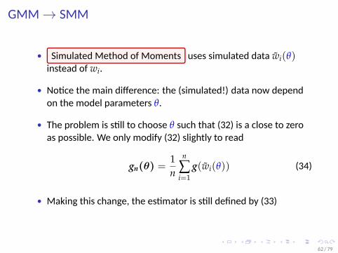
GMM→ SMM• Simulated Method of Moments uses simulated data wi(θ)instead of wi.• No�ce the main difference: the (simulated!) data now dependon the model parameters θ.• The problem is s�ll to choose θ such that (32) is a close to zeroas possible. We only modify (32) slightly to read

gn(θ) =1n

n

∑i=1

g(wi(θ)) (34)

• Making this change, the es�mator is s�ll defined by (33)

62 / 79

SMM Prac�cali�es

• No�ce that obtaining a sample of simulated data {wi(θ)}Ni=1involves

1 Solving the dynamic program (30), Vt(Xt, θ)2 Using the op�mal policies, simula�ng a panel of data.

where step 1 usually is costly in terms of computa�on �me.• The precise form of the moment func�on g is, to some extent,at the researcher’s discre�on.• Which moments to include in g is a similar ques�on to whichvariables to include in my regression.

63 / 79

French (2005): Moment Func�on g

The moments the model must match are:1 Median assetes2 Mean assets3 Mean par�cipa�on condi�onal on health4 Mean hours condi�onal on health

See Equa�ons (14)-(17) in the paper for how those are computed.

64 / 79

Es�ma�ng Lifecycle Profiles from Data• If t indexes calendar �me and i individuals, define a genericlifecycle profile of variable x by

E[xit|agei] (35)• Wri�en as in (35), this contains individual fixed effects, yeareffects and family size effects. A complicated object to interpret.• Probably be�er would be

E[xit|agei, t, i, Mit, famsizeit]

Ques�on: How is this condi�onal expecta�on iden�fied?

65 / 79

Es�ma�ng Lifecycle Profiles from Data

• To address those issues, French proposesZit = fi + ∑

m∈good,badT

∑k=1

Πmk1[ageit = k|m]

+J

∑j=1

1[famsizeit = j] + ΠUUt + uit

where Z stands for assets, hours, par�cipa�on or wages.• The required age profiles are the sequences of paramters

∑Tk=1 Πmk.

66 / 79

Selected Wage Data

• A problem with this is that wage data is only observed forworkers.• Classical Ques�on: What about the wage of non-workers? Thisis really like in Heckman (1977).• If wage growth were the same for workers and non-workers, thiswould not be a problem – the fixed effect es�mator iden�fieswage growth.• French (2005) proposes to compare selec�on bias in real andsimulated data in an itera�ve proceedure.

67 / 79

Data

• Panel Study of Income Dynamics (PSID) 1968–1997.• Rich income data, assets in several waves, labor supply, and alsohealth data are included.• PSID is a great dataset to work with.• https://cran.r-project.org/web/packages/psidR/

index.html is a great package to build it.

68 / 79

https://cran.r-project.org/web/packages/psidR/index.html

https://cran.r-project.org/web/packages/psidR/index.html



69 / 79

Results: Exogenous profiles 1

70 / 79

Results: Exogenous profiles 2

71 / 79

Results: Parameter Es�mates

72 / 79

Results: Model Fit 1

73 / 79


74 / 79

Experiments

Baseline (1987 policy environment) vs1 Redues SS benefits by 20%2 Increase early re�rement age from 62 to 63.3 Eliminate SS earnings test for over 65 year olds.4 Earnings test was in fact abolished in 2000 - look at modelpredic�ons.

75 / 79

Results: Policy Experiments

76 / 79


• Removing earnings test increases life�me wealth.• Leisure being normal good, this increases demand for C as wellas L• Hence par�cipate for more years.

77 / 79


• Removing earnings test increases life�me wealth.• Leisure being normal good, this increases demand for C as wellas L• Hence par�cipate for more years.

77 / 79

Conclusions

• French (2005) constructs an es�mable lifecycle model withlabour supply, re�rement, savings and social security.• People would spend 3 months more in work if SS weredecreased by 30%.• The sharp drop in par�cipa�on at age 65 is explained byactuarial unfairness of pension and SS around that age.

78 / 79

ReferencesJerome Adda and Russell W Cooper. Dynamic economics:quan�ta�ve methods and applica�ons. MIT press, 2003.

Lars Ljungqvist and Thomas J Sargent. Recursive macroeconomictheory. MIT press, 2012.

RE Lucas and NL Stokey. Recursive Methods in Dynamic Economics.Harvard University Press, Cambridge MA, 1989.Eric French. The effects of health, wealth, and wages on laboursupply and re�rement behaviour. The Review of Economic Studies,72(2):395–427, 2005. ISSN 00346527. URLhttp://www.jstor.org/stable/3700657.

James J Heckman. Sample selec�on bias as a specifica�on error (withan applica�on to the es�ma�on of labor supply func�ons), 1977.

79 / 79

http://www.jstor.org/stable/3700657

Documents

Introduc„on to Dynamic Programming and Applica„on from Erich … · Applica„on from Erich French (2005) ScPo Graduate Labor February 23, 2017 1/79. Table of contents Dynamic