INTRODUCTION TO MICROECONOMICS

Graphs and Tables

Part #3

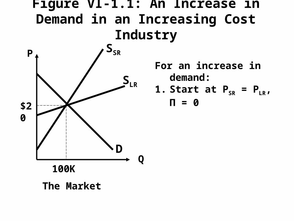
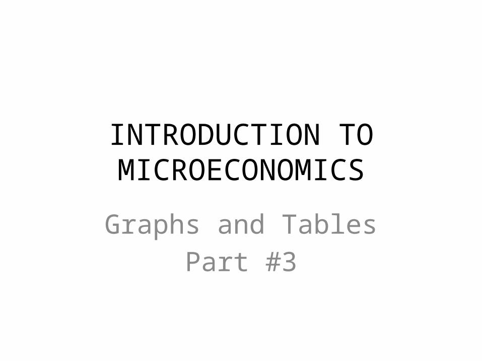
Figure VI-1.1: An Increase in Demand in an Increasing Cost Industry

D

SSR

$20

100K

The Market

Q

P

SLR

For an increase in demand:1. Start at PSR = PLR, Π = 0

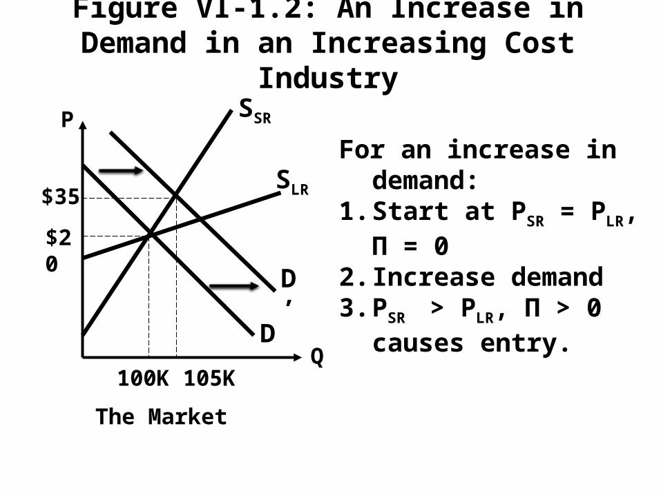
Figure VI-1.2: An Increase in Demand in an Increasing Cost Industry

D

SSR

$20

100K 105K

The Market

Q

P

D’

$35SLR

For an increase in demand:1. Start at PSR = PLR, Π = 02. Increase demand3. PSR > PLR, Π > 0 causes

entry.

Figure VI-1.3: An Increase in Demand in an Increasing Cost Industry

D

SSR

$20

100K 105K110K

The Market

Q

P

D’

$35

S’SR

SLR

$30

For an increase in demand:1. Start at PSR = PLR, Π = 02. Increase demand3. PSR > PLR, Π > 0 causes

entry.4. Entry causes S to

increase.5. Costs also increase and P decreases until PSR =

PLR and Π = 0 (back in LR equilibrium).

Figure VI-1.5: A Technological Change in an Increasing Cost Industry

D

SSR

$20

100K 110K

The Market

Q

P

SLR

1. Start at PSR = PLR, Π = 02. SLR Shift to the Right3. PSR > PLR, Π > 0 causes

entry.S’LR $15

Figure VI-1.6: A Technological Change in an Increasing Cost Industry

D

SSR

$20

100K 110K

The Market

Q

P

SLR

1. Start at PSR = PLR, Π = 02. SLR Shift to the Right3. PSR > PLR, Π > 0 causes

entry.4. SSR Increases Until PSR

= PLR, Π = 0

S’LR $15

Figure VI-1.3: An Increase in Demand in an Increasing Cost Industry

D

SSR

$20

100K 105K110K

The Market

Q

P

D’

$35

S’SR

SLR

$30

For an increase in demand:1. Start at PSR = PLR, Π = 02. Increase demand3. PSR > PLR, Π > 0 causes

entry.4. Entry causes S to

increase.5. Costs also increase and P decreases until PSR =

PLR and Π = 0 (back in LR equilibrium).

Figure VI-2.1: An Increase in Demand in an Increasing Cost Industry with Legal Entry

Barriers

D

SSR

$20

100K

The Market

Q

P

SLR

For an increase in demand:1. Start at PSR = PLR, Π = 0;

Legal Entry Barriers Imposed Here

Figure VI-2.2: An Increase in Demand in an Increasing Cost Industry with Legal Entry

Barriers

D

SSR

$20

100K 105K 110K

The Market

Q

P

D’

$35SLR

For an increase in demand:1. Start at PSR = PLR, Π = 02. Increase demand3. PSR > PLR, Π > 0 but

entry is blocked so existing firms are able to earn Π > 0 .

Table VI-4: The Market for Wheat with Price Support

P QDPVT QD

PVT + USDA QS

$0.00 130 190 **

$2.00 120 180 00

$4.00 110 170 20

$6.00 100 160 40

$8.00 90 150 60

$10.00 80 140 80

$12.00 70 130 100

PSUP $14.00 60 120 120

$16.00 50 110 140

$18.00 40 100 160

$20.00 30 90 180

Figure VI-4: The Market for Wheat with Price Supports

P

Q

S

DPVT

$10

$26

$2

60 80 120

PSUP = $14 DPVT + USDA

ES

Consumers pay = $14(60) = $840USDA pays = $14(120 – 60) = $840

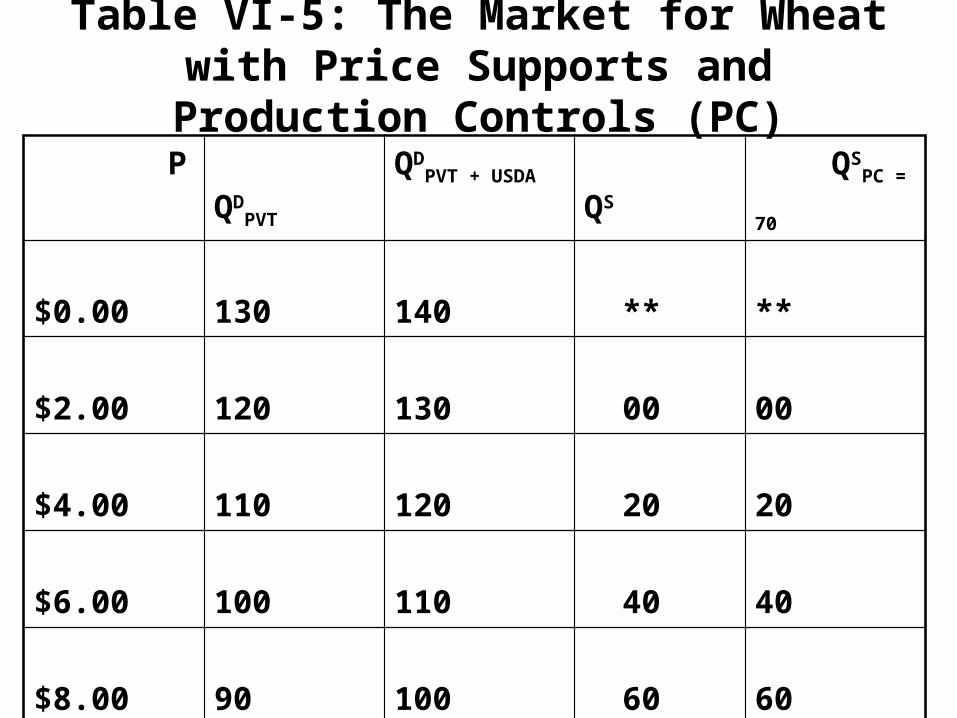
Table VI-5: The Market for Wheat with Price Supports and Production Controls (PC)

P QDPVT QD

PVT + USDA QS QS

PC = 70

$0.00 130 140 ** **

$2.00 120 130 00 00

$4.00 110 120 20 20

$6.00 100 110 40 40

$8.00 90 100 60 60

$10.00 80 90 80 70

$12.00 70 80 100 70

*$14.00 60 70 120 70

$16.00 50 60 140 70

$18.00 40 50 160 70

$20.00 30 40 180 70

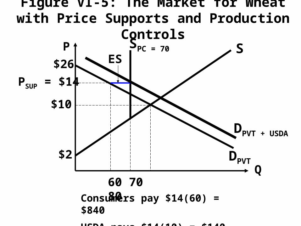
Figure VI-5: The Market for Wheat with Price Supports and Production Controls

P

Q

S

DPVT

$10

$26

$2

60 70 80

PSUP = $14

SPC = 70

ES

DPVT + USDA

Consumers pay $14(60) = $840

USDA pays $14(10) = $140

Table VI-6: Target Prices

P QDPVT QS

$0.00 130 **

PCON $2.00 *120 00

$4.00 110 20

$6.00 100 40

$8.00 90 60

$10.00 80 80

$12.00 70 100

PTAR $14.00 60 *120

$16.00 50 140

$18.00 40 160

$20.00 30 180

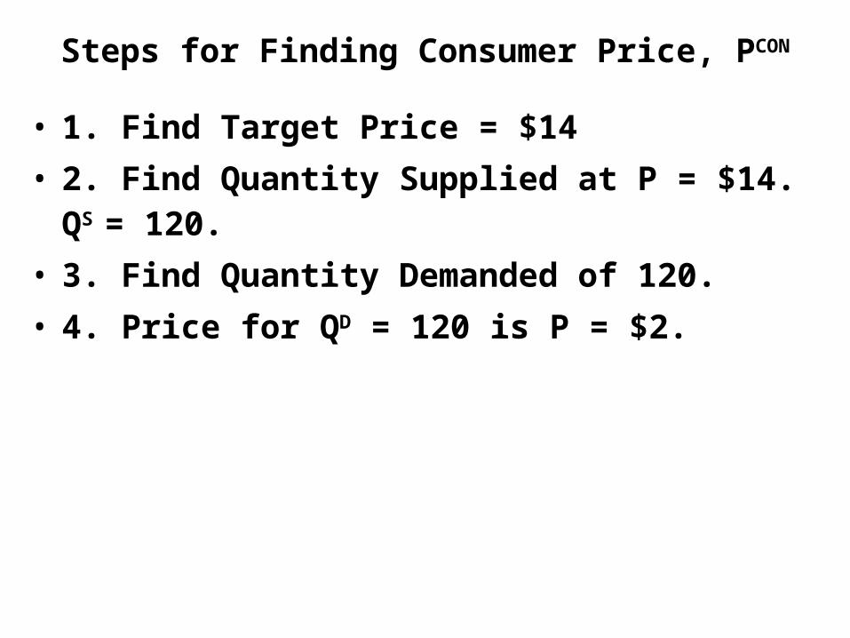
Steps for Finding Consumer Price, PCON

• 1. Find Target Price = $14• 2. Find Quantity Supplied at P = $14. QS = 120.• 3. Find Quantity Demanded of 120.• 4. Price for QD = 120 is P = $2.

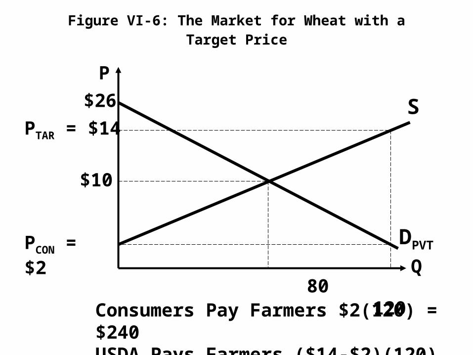
Figure VI-6: The Market for Wheat with a Target Price

P

Q

S

DPVT

$10

$26

PCON = $2

80 120

PTAR = $14

Consumers Pay Farmers $2(120) = $240USDA Pays Farmers ($14-$2)(120) = $1,440

Figure VI-7: The Welfare Loss in a Market for Wheat with a Target Price

P

Q

S

DPVT

$10

$26

PCON = $2

80 120

PTAR = $14

WL

WL = ½(b)(h) = ½ $12(40) = $240

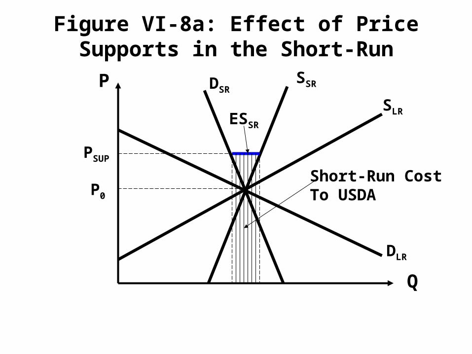
Figure VI-8a: Effect of Price Supports in the Short-Run

ESSR

DSRSSR

SLR

DLR

Short-Run CostTo USDA

P

Q

P0

PSUP

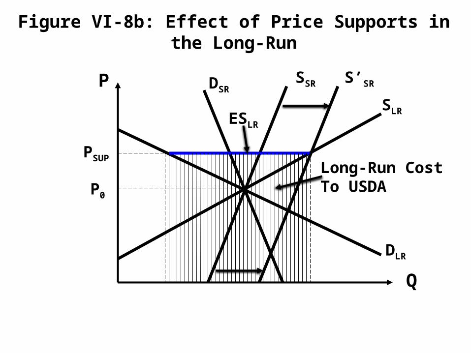
Figure VI-8b: Effect of Price Supports in the Long-Run

ESLR

DSRSSR

SLR

DLR

P

Q

P0

PSUP

S’SR

Long-Run CostTo USDA

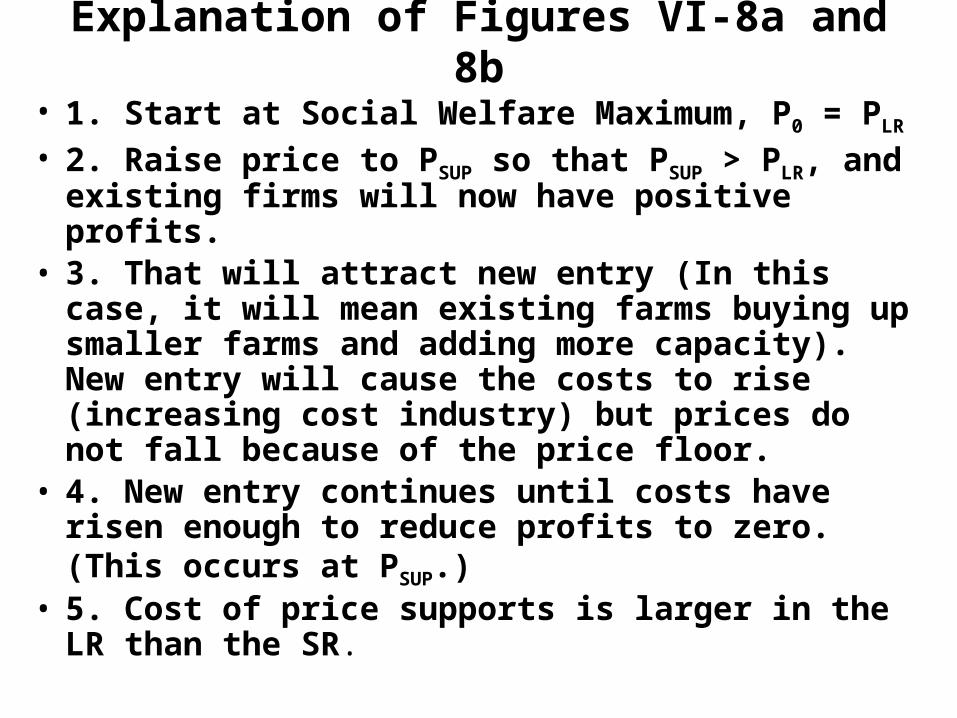
Explanation of Figures VI-8a and 8b

• 1. Start at Social Welfare Maximum, P0 = PLR

• 2. Raise price to PSUP so that PSUP > PLR, and existing firms will now have positive profits.

• 3. That will attract new entry (In this case, it will mean existing farms buying up smaller farms and adding more capacity). New entry will cause the costs to rise (increasing cost industry) but prices do not fall because of the price floor.

• 4. New entry continues until costs have risen enough to reduce profits to zero. (This occurs at PSUP.)

• 5. Cost of price supports is larger in the LR than the SR.

Figure VI-9: Effect of a Producer Subsidy• Subsidy to producers results in misallocation of

resources: Too much output in subsidized Market and too little output in the Rest of Economy

Rest of Economy FarmMarkets

Farm Subsidy

Resources

Output Increases Output Decreases

(Lower Valued Use)

Farm Subsidy in Farm Markets is equivalent to a tax on the Rest of Economy

Figure VI-10: The Market for Corn--Supply and Demand Curves

P

Q

S

D

$10.00

$26.00

$2.00

100K

a

PF = $14.00

b

c