Embed Size (px)
Citation preview
1
Introduction to Structural
Equation Modeling
Hsueh-Sheng Wu
CFDR Workshop Series
Summer 2009
2
Outline of Presentation
• Basic concepts of structural equation model (SEM)
• What are advantages of SEM over OLS?
• Steps of fitting SEM
• An example of fitting SEM
• Different types of SEM
• Strengths and Limitations of SEM
• Conclusions
3
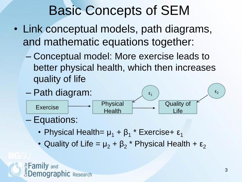
Basic Concepts of SEM
• Link conceptual models, path diagrams,
and mathematic equations together:
– Conceptual model: More exercise leads to
better physical health, which then increases
quality of life
– Path diagram:
– Equations:
• Physical Health= μ1 + β1 * Exercise+ ε1
• Quality of Life = μ2 + β2 * Physical Health + ε2
ExercisePhysical
Health
Quality of
Life
ε1ε2
Jargon of SEM
• Variables in SEM
– Measured variable
– Latent variable
– Exogenous variable
– Endogenous variable
– Error
– Disturbance
4
Relation between Two Variables
• A path with a single headed arrow
– one variable predicts the other variable
– one variable is the indicator of the other
variable
• A path with a double-headed arrow means
that two variables are correlated with each
other
• No path means no direct relation between two
variables
5
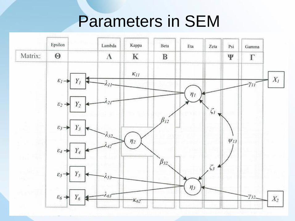
Parameters in SEM
6
Effects of One Variable on Another
Variable
• Direct effect
• Indirect effect
• Total effect
7
8
Advantages of SEM over OLS• Control for measurement errors in observed independent
variables, dependent variables, or both.
• Analyze more than one dependent variables at a time
• Distinguish among direct, indirect, and total effects of
variables
• Model how Xs influence Ys via other variables
• Test more complex models on three or more waves of
longitudinal data
9
Steps of Conducting SEM Analysis• Develop a theoretically based model
• Construct the SEM diagram
• Convert the SEM diagram into a set of structural
equations
• Clean data and decide the input data type
• Determine the estimation method
• Run the model and evaluate goodness-of-fit of
the model
• Modify the model
• Compare two models and decide if additional
modification is needed
10
Input Data Type
• Raw data
• Correlation matrix
• Covariance matrix
• Covariance matrix and means
• Correlation matrix and standard deviations
• Correlation matrix, standard deviations,
and means
11
Estimation Methods
• ML: Maximum likelihood estimation
• ULS: unweighted least squares estimation
• GLS: generalized least squares estimation
12
Maximum Likelihood Estimation• Assume multivariate normality of observed
variables
• Is commonly used with large sample size
• Parameter estimates are consistent,
asymptotically unbiased, and efficient
• Estimates are normally distributed, which
allows for testing statistical significance of
parameters
• ML estimates are scale-free
13
Unweighted Least Squares Estimation
• Statistically consistent parameter estimates
• No distributional assumption for variables
• Possibly compute tests of significance for
model parameter
• Item parameter estimates and fit index are
scale dependent
• Parameter estimates are not asymptotically
efficient
• No overall test of fit
14
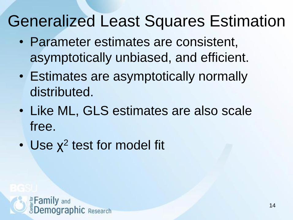
Generalized Least Squares Estimation
• Parameter estimates are consistent,
asymptotically unbiased, and efficient.
• Estimates are asymptotically normally
distributed.
• Like ML, GLS estimates are also scale
free.
• Use χ2 test for model fit
15
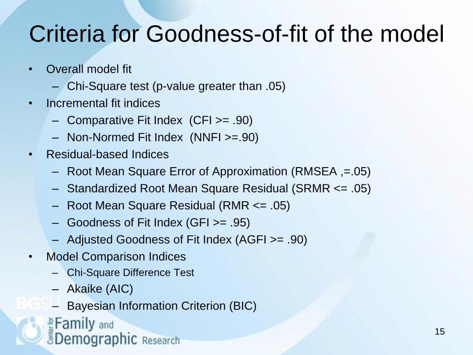
Criteria for Goodness-of-fit of the model
• Overall model fit
– Chi-Square test (p-value greater than .05)
• Incremental fit indices
– Comparative Fit Index (CFI >= .90)
– Non-Normed Fit Index (NNFI >=.90)
• Residual-based Indices
– Root Mean Square Error of Approximation (RMSEA ,=.05)
– Standardized Root Mean Square Residual (SRMR <= .05)
– Root Mean Square Residual (RMR <= .05)
– Goodness of Fit Index (GFI >= .95)
– Adjusted Goodness of Fit Index (AGFI >= .90)
• Model Comparison Indices
– Chi-Square Difference Test
– Akaike (AIC)
– Bayesian Information Criterion (BIC)
16
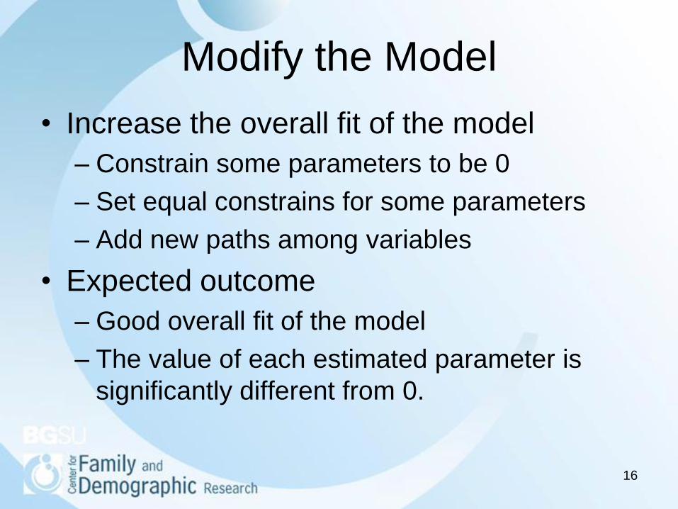
Modify the Model
• Increase the overall fit of the model
– Constrain some parameters to be 0
– Set equal constrains for some parameters
– Add new paths among variables
• Expected outcome
– Good overall fit of the model
– The value of each estimated parameter is
significantly different from 0.
17
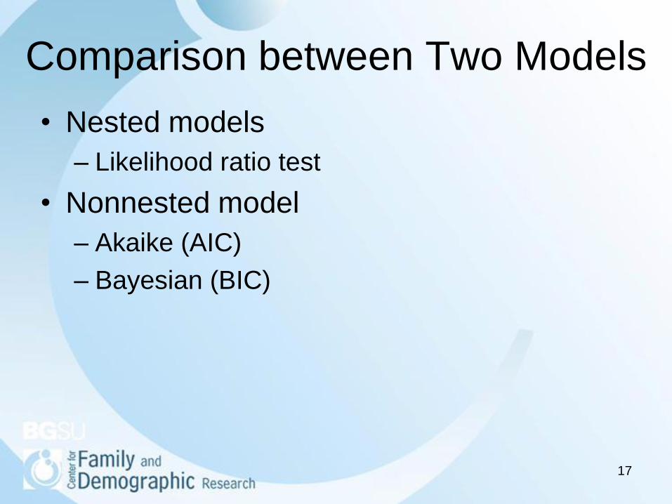
Comparison between Two Models
• Nested models
– Likelihood ratio test
• Nonnested model
– Akaike (AIC)
– Bayesian (BIC)
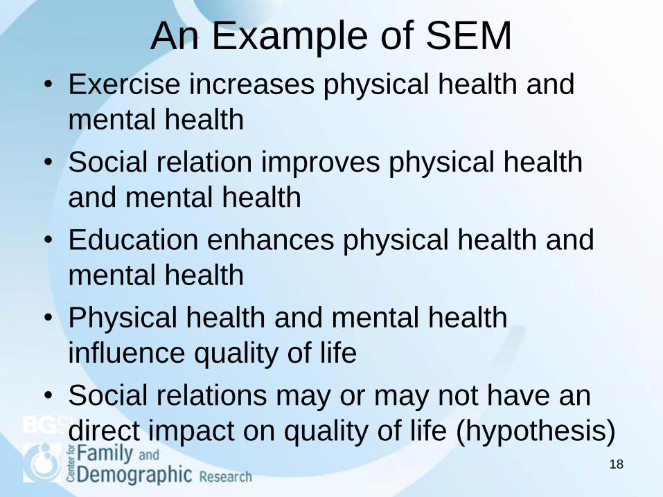
18
An Example of SEM• Exercise increases physical health and
mental health
• Social relation improves physical health
and mental health
• Education enhances physical health and
mental health
• Physical health and mental health
influence quality of life
• Social relations may or may not have an
direct impact on quality of life (hypothesis)
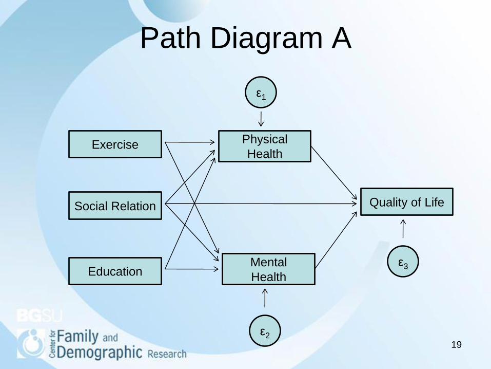
19
Path Diagram A
Exercise
Social Relation
Education
Physical
Health
Quality of Life
Mental
Health
ε1
ε2
ε3

20
Path Diagram B
Exercise
Social Relation
Education
Physical
Health
Quality of Life
Mental
Health
ε1
ε2
ε3
21
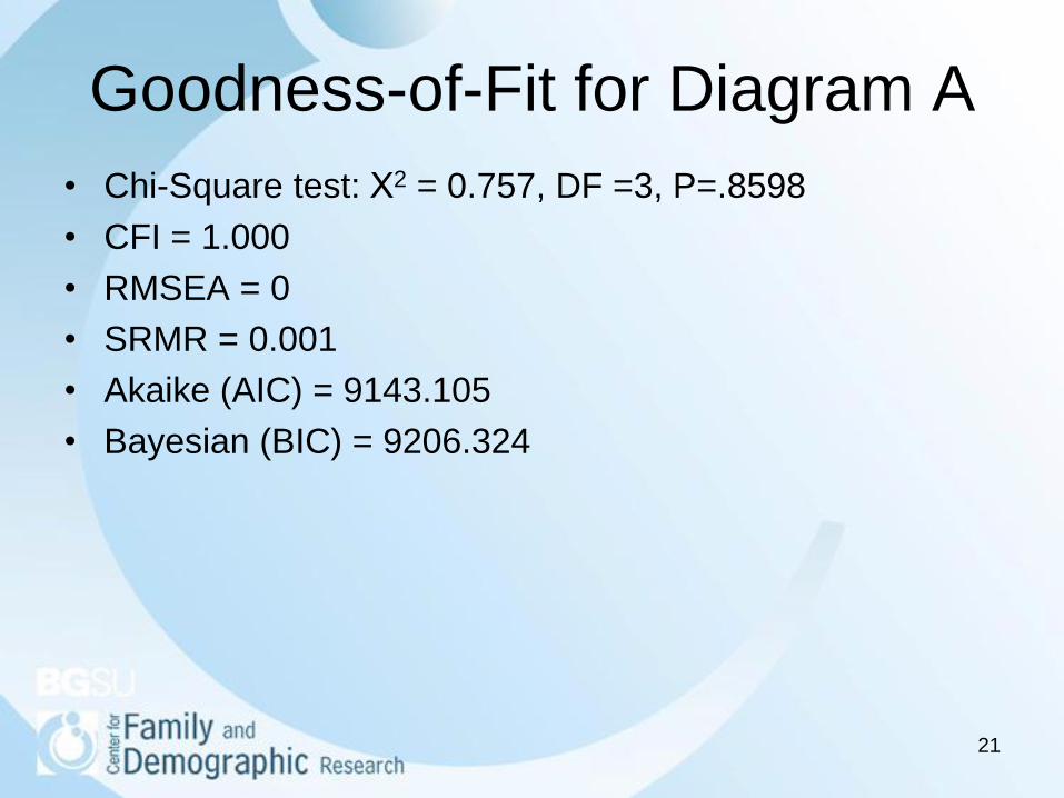
Goodness-of-Fit for Diagram A
• Chi-Square test: Χ2 = 0.757, DF =3, P=.8598
• CFI = 1.000
• RMSEA = 0
• SRMR = 0.001
• Akaike (AIC) = 9143.105
• Bayesian (BIC) = 9206.324
22
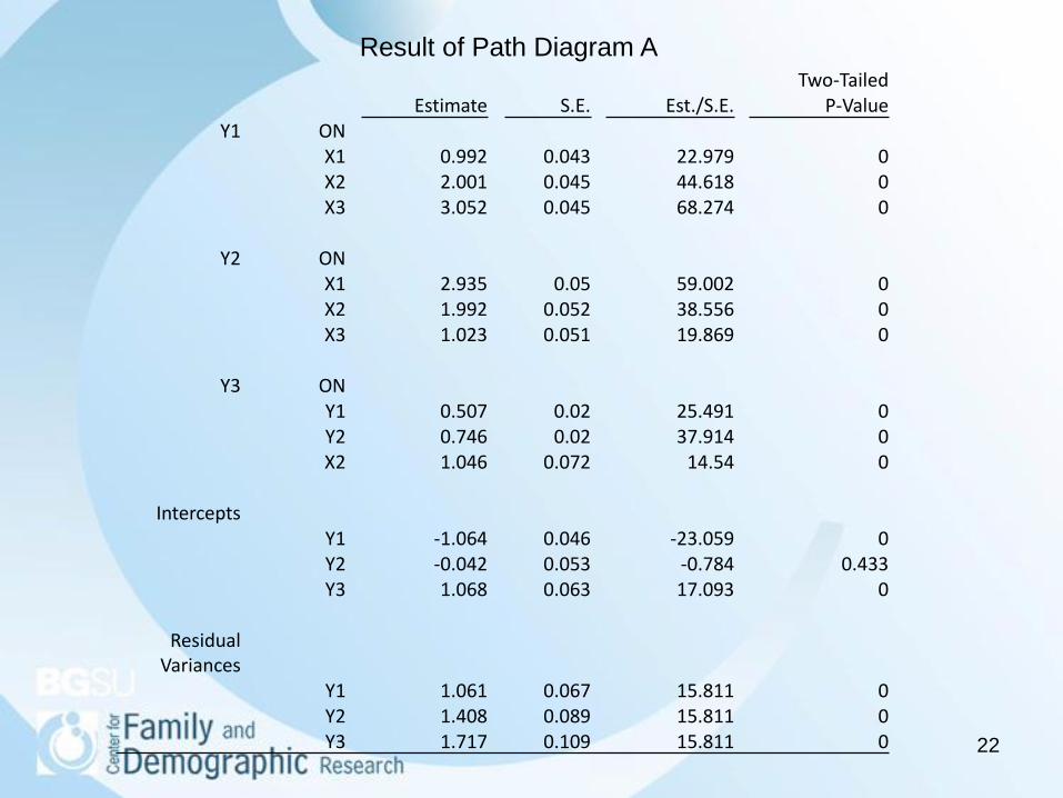
Two-TailedEstimate S.E. Est./S.E. P-Value
Y1 ONX1 0.992 0.043 22.979 0X2 2.001 0.045 44.618 0X3 3.052 0.045 68.274 0
Y2 ONX1 2.935 0.05 59.002 0X2 1.992 0.052 38.556 0X3 1.023 0.051 19.869 0
Y3 ONY1 0.507 0.02 25.491 0Y2 0.746 0.02 37.914 0X2 1.046 0.072 14.54 0
InterceptsY1 -1.064 0.046 -23.059 0Y2 -0.042 0.053 -0.784 0.433Y3 1.068 0.063 17.093 0
Residual Variances
Y1 1.061 0.067 15.811 0Y2 1.408 0.089 15.811 0Y3 1.717 0.109 15.811 0
Result of Path Diagram A
23
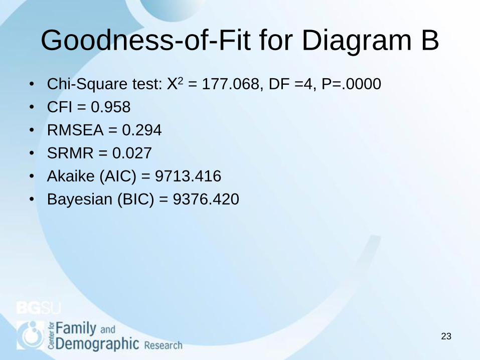
Goodness-of-Fit for Diagram B
• Chi-Square test: Χ2 = 177.068, DF =4, P=.0000
• CFI = 0.958
• RMSEA = 0.294
• SRMR = 0.027
• Akaike (AIC) = 9713.416
• Bayesian (BIC) = 9376.420
24
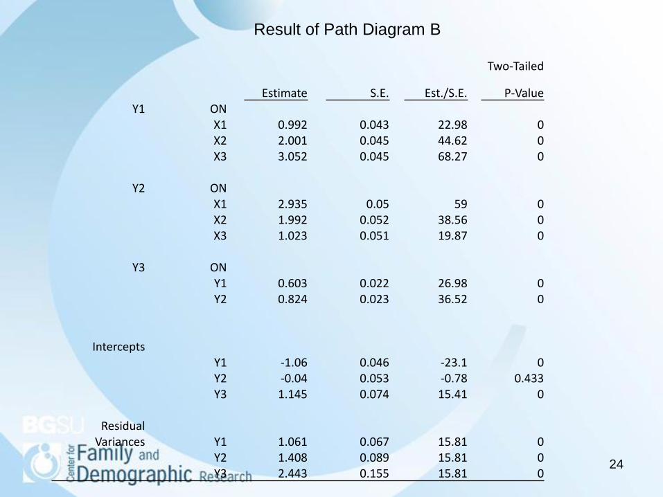
Result of Path Diagram B
Two-Tailed
Estimate S.E. Est./S.E. P-ValueY1 ON
X1 0.992 0.043 22.98 0X2 2.001 0.045 44.62 0X3 3.052 0.045 68.27 0
Y2 ONX1 2.935 0.05 59 0X2 1.992 0.052 38.56 0X3 1.023 0.051 19.87 0
Y3 ONY1 0.603 0.022 26.98 0Y2 0.824 0.023 36.52 0
InterceptsY1 -1.06 0.046 -23.1 0Y2 -0.04 0.053 -0.78 0.433Y3 1.145 0.074 15.41 0
Residual Variances Y1 1.061 0.067 15.81 0
Y2 1.408 0.089 15.81 0Y3 2.443 0.155 15.81 0
25
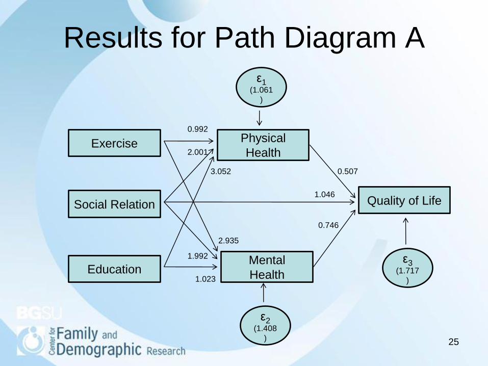
Results for Path Diagram A
Exercise
Social Relation
Education
Physical
Health
Quality of Life
Mental
Health
ε1(1.061
)
0.992
0.507
2.935
2.001
3.052
1.046
0.746
1.023
1.992
ε2(1.408
)
ε3(1.717
)
26
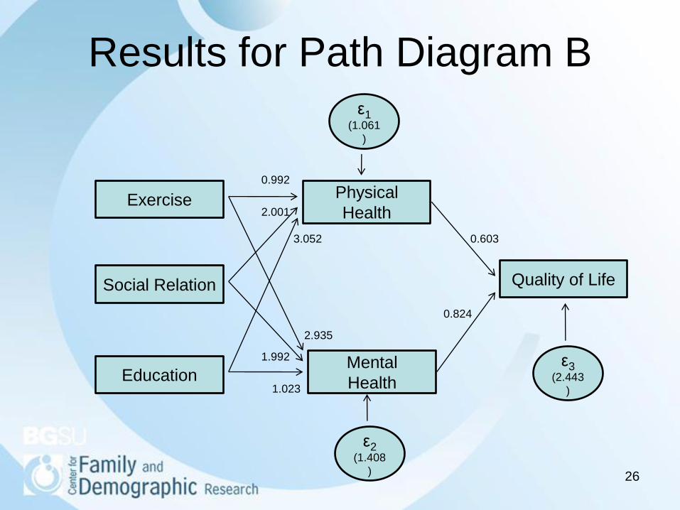
Results for Path Diagram B
Exercise
Social Relation
Education
Physical
Health
Quality of Life
Mental
Health
ε1(1.061
)
0.992
0.603
2.935
2.001
3.052
0.824
1.023
1.992
ε2(1.408
)
ε3(2.443
)
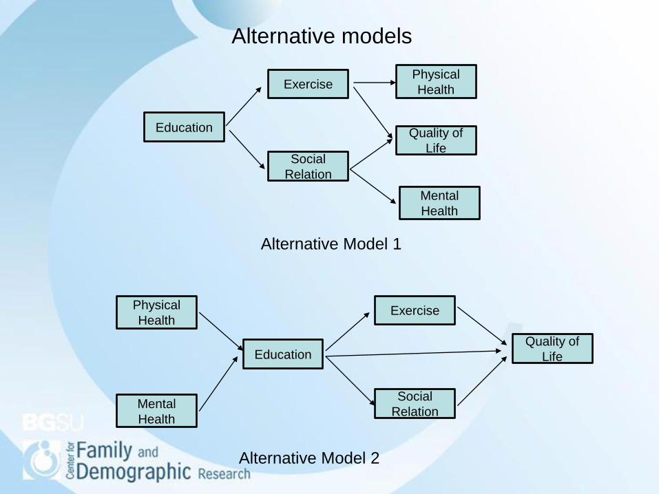
Alternative models
Exercise
Social
Relation
Education
Physical
Health
Quality of
Life
Mental
Health
Exercise
Social
Relation
Education
Physical
Health
Quality of
Life
Mental
Health
Alternative Model 2
Alternative Model 1
28
Different Types of SEM
• Path model
• Auto-regressive model
• Growth curve model
• Hierarchical linear model
• Mixture model
• Latent class analysis
29
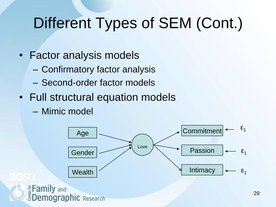
Different Types of SEM (Cont.)
• Factor analysis models
– Confirmatory factor analysis
– Second-order factor models
• Full structural equation models
– Mimic model
Love
Age
Wealth
Gender
Commitment
Intimacy
Passion
ε1
ε1
ε1
A Few SEM Applications in JMF
• Schoppe-Sullivan, Sarah J, Alice C. Schermerhorn, and E.
Mark Cummings. 2007. “Marital Conflict and Children’s
Adjustment: Evaluation of the Parenting Process Model.”
Journal of Marriage and Family 69: 1118-1134.
• Vandewater, Elizabeth A. and Jennifer E. Lansford. 2005.
“A Family Process Model of Problem Behaviors in
Adolescents.” Journal of Marriage and Family 67: 100-109.
• Mistry, Rashmita S., Edward D. Lowe, Aprile D. Benner,
and Nina Chien. 2008. “Expanding the Family Economic
Stress Model: Insights from a Mixed-Methods Approach.”
Journal of Marriage and Family 70: 196-209.
30
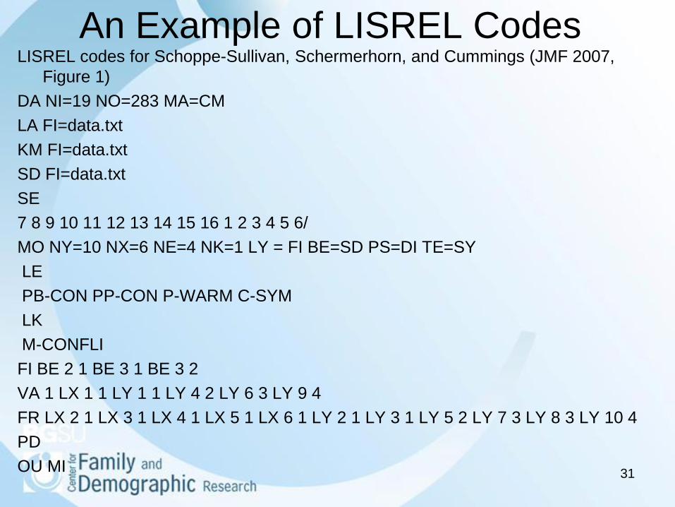
An Example of LISREL CodesLISREL codes for Schoppe-Sullivan, Schermerhorn, and Cummings (JMF 2007,
Figure 1)
DA NI=19 NO=283 MA=CM
LA FI=data.txt
KM FI=data.txt
SD FI=data.txt
SE
7 8 9 10 11 12 13 14 15 16 1 2 3 4 5 6/
MO NY=10 NX=6 NE=4 NK=1 LY = FI BE=SD PS=DI TE=SY
LE
PB-CON PP-CON P-WARM C-SYM
LK
M-CONFLI
FI BE 2 1 BE 3 1 BE 3 2
VA 1 LX 1 1 LY 1 1 LY 4 2 LY 6 3 LY 9 4
FR LX 2 1 LX 3 1 LX 4 1 LX 5 1 LX 6 1 LY 2 1 LY 3 1 LY 5 2 LY 7 3 LY 8 3 LY 10 4
PD
OU MI 31
32
Strengths of SEM• Specify various models for different
relations among variables, depending on theoretical frameworks
• Distinguish among direct, indirect, and total effect of variables
• Analyze the relations among variables controlling for measurement errors
• Comprehensive statistical tests for identifying and comparing different structural models
33
Limitations of SEM
• SEM does not establish causal orders
among variables if the temporal order of
these variables is unknown.
• Missing data and outliers influence the
covariance and correlation matrices
analyzed.
34
Limitations of SEM (Cont.)
• A large sample size produces stable
estimates of the covariance or correlation
among variables, but it make the model
easier to be rejected.
• There may be multiple equivalent models
that fit data equally well.
• The number of parameters to be estimated
cannot exceed the number of known
values.
35
Conclusions• SEM is a useful analytic technique in situations
when independent variables, dependent variables,
or both contain measurement errors.
• Even when your variables do not contain
measurement errors, SEM allows for better testing
theoretical links (i.e., paths) among variables.
• Available software: SAS, LISREL, Amos, EQS,
and Mplus.
– SAS is available on all computers in Williams Hall.
– LISREL is available in Hayes 025 Lab and Olscamp
207 Lab.
– Amos, EQS, and Mplus not supported by BGSU
36
Conclusions (Cont.)• More readings about SEM:
Bollen (1989, Structural Equation Modeling)
Kline (1998, Principles and Practice of Structural
Equation Modeling)
Kaplan (2000, Structural equation Modeling)
Raykov & Marcoulides (2000, A First Course in
Structural Equation Modeling)
• If you encounter problems running SEM models,
feel free to contact me (Hsueh-Sheng Wu,
[email protected], 419-372-3119).