Introduction to the Economics of

Introduction to the Economics of Financial Markets

This page intentionally left blank

Introduction to theEconomics of FinancialMarkets

James Bradfield

12007

1Oxford University Press, Inc., publishes works that furtherOxford University’s objective of excellencein research, scholarship, and education.

Oxford New YorkAuckland Cape Town Dar es Salaam Hong Kong KarachiKuala Lumpur Madrid Melbourne Mexico City NairobiNew Delhi Shanghai Taipei Toronto

With offices inArgentina Austria Brazil Chile Czech Republic France GreeceGuatemala Hungary Italy Japan Poland Portugal SingaporeSouth Korea Switzerland Thailand Turkey Ukraine Vietnam

Copyright © 2007 by Oxford University Press

Published by Oxford University Press, Inc.198 Madison Avenue, New York, New York 10016

www.oup.com

Oxford is a registered trademark of Oxford University Press

All rights reserved. No part of this publication may be reproduced,stored in a retrieval system, or transmitted, in any form or by any means,electronic, mechanical, photocopying, recording, or otherwise,without the prior permission of Oxford University Press.

Library of Congress Cataloging-in-Publication DataBradfield, James.

Introduction to the economics of financial markets / James Bradfield.p. cm.

Includes bibliographical references and index.ISBN-13 978-0-19-531063-4ISBN 0-19-531063-21. Finance. 2. Capital market. I. Title.HG173.B67 2007332—dc22 2006011610

9 8 7 6 5 4 3 2 1Printed in the United State of Americaon acid-free paper

www.oup.com

To my wife, Alice, to our children, and to their children

To the memory of Professor Edward Zabel, a friend and mentor, who taught me the importance of

extracting the economic interpretations from the mathematics, and who taught me much more.


My greatest debt is to my wife, Alice, whose encouragement, understanding, and clearthinking about choices are indefatigable.

Most professors owe much to their students; I am no exception. I have learnedmuch from the students who have taken the courses from which I have drawn this book.Several of those students read many drafts of the book, eliminated errors, and madevaluable suggestions for additional examples and for clarity of exposition. I thank JohnBalio, Tierney Boisvert, Katherine E. Brogan, Matt Clausen, Mike Coffey, KaitieDonovan, Matt Drescher, John Durland, Schuyler Gellatly, Young Han, Tom Heacock,Jason Hong, Danielle Levine, Brendan Mahoney, Abhishek Maity, Katie Nedrow,Quang Nguyen, Greg Noel, Cy Philbrick, Brad Polan, Eric Reile, Dan Rubin, KatieSarris, Kevin St. John, Gregory Scott, Joseph P. H. Sullivan, and Kimberly Walker. Iappreciate the work of Rachael Arnold, who used her skills as a graphic artist to createcomputerized drawings of the several figures.

I thank Dawn Woodward for the numerous times that she assisted me with thearcana of word processing, and for many other instances of secretarial assistance.

Five former students served (seriatim) as editorial and research assistants. I amgrateful to Mo Berkowitz, Jon Farber, Gregory H. Jaske, Kathleen McGrory, and MacWeiss for their industriousness, their intelligence, and their constant good cheer. Eachof them contributed significantly to this book.

I extend appreciation especially to Dr. Janette S. Albrecht, who watched theprogress of this book through periods of turbulence, and who added several dimen-sions to my understanding of sunk costs.

Mrs. Ann Burns, a friend of long standing from my days in the dean’s office,cheerfully, speedily, and accurately typed numerous drafts of the manuscript, many ofwhich I wrote by hand, with labyrinthian notes (in multiple colors) in the margins andon the back sides of preceding and succeeding pages. I wish Ann and her family well.

I thank Mike Mercier for his editorial encouragement and guidance during anearlier incarnation of this book.

My friend and colleague, Professor of English George H. Bahlke, who is anexpert on twentieth-century British literature, helped me to maintain a greater meas-ure of equanimity than I would have had without his support.

I am also indebted to my friend and colleague, Professor of History Robert L.Paquette, who has written extensively on the Atlantic slave trade, and with whom

Acknowledgments

I teach a seminar on property rights and the rise of the modern state. Among other valu-able lessons, Professor Paquette reminded me on several occasions that the applicationof theoretical models in economics is limited by the prejudices of the persons whosebehavior we are trying to explain.

I appreciate the confidence that Terry Vaughn, Executive Editor at OxfordUniversity Press, expressed in my work, which culminated in this book. CatherineRae, the assistant to Mr. Vaughn, helped me in numerous ways as I responded to referees’ suggestions and prepared the manuscript. Stephania Attia, the ProductionEditor for this book, supervised the compositing closely, and I thank her for doing so.I also appreciate the attention to detail provided by Jean Blackburn of BythewayPublishing Services. Judith Kip, a professional indexer, contributed significantly byconstructing the index.

Acknowledgmentsviii

This book is an introductory exposition of the way in which economists analyze how,and how well, financial markets organize the intertemporal allocation of scarceresources. The central theme is that the function of a system of financial markets is toenable consumers, investors, and managers of firms to effect mutually beneficialintertemporal exchanges. I use the standard concept of economic efficiency (Paretooptimality) to assess the efficacy of the financial markets. I present an intuitive devel-opment of the primary theoretical and empirical models that economists use to analyzefinancial markets. I then use these models to discuss implications for public policy.

The book presents the economics of financial markets; it is not a text in corporatefinance, managerial finance, or investments in the usual senses of those terms. Therelationship between a course for which this book is written, and courses in corporatefinance and investments, is analogous to the relationship between a standard course inmicroeconomics and a course in managerial economics.

I emphasize concrete, intuitive interpretations of the economic analysis. Myobjective is to enable students to recognize how the theoretical and empirical resultsthat economists have established for financial markets are built on the central eco-nomic principles of equilibrium in competitive markets, opportunity costs, diversifi-cation, arbitrage, and trade-offs between risk and expected return. I develop carefullythe logic that supports and organizes these results, leaving the derivation of rigorousproofs from first principles to advanced texts. (Some proofs and technical extensionsare presented in appendices to some of the chapters.) Students who use this text willacquire an understanding of the economics of financial markets that will enable themto read with some sophistication articles in the public press about financial marketsand about public policy toward those markets. Dedicated readers will be able tounderstand the central issues and the results (if not the technical methods) in the schol-arly literature.

I address the book primarily to undergraduate students. The selection and presen-tation of topics reflect the author’s long experience teaching in the Department ofEconomics at Hamilton College. Undergraduate and beginning graduate students inprograms of business administration who want an understanding of how economistsassess financial markets against the criteria of allocative and informational efficiencywill also find this book useful.

Preface

I have taught mainly in the areas of investments and portfolio theory, and in intro-ductory and intermediate microeconomic theory. I also teach a course in mathemati-cal economics, and I have written (with Jeffrey Baldani and Robert Turner, who areeconomists at Colgate University) the text Mathematical Economics, second edition(2005). I recently taught an introductory course and an advanced seminar in mathe-matical economics at Colgate.

Readers of this book should have completed one introductory course in econom-ics (preferably microeconomics). Although I use elementary concepts in probabilityand statistics, it is not critical that readers have completed formal courses in theseareas. I present in the text the concepts in probability and statistics that will enable astudent with no previous work in these areas to understand the economic analysis.Students who have completed an introductory course in probability and statistics willbe able to understand the exposition in the text more easily. I use graphs extensively,and I assume that students understand the solution of pairs of linear equations.

Prefacex

Part I Introduction

1 The Economics of Financial Markets 3

1.1 The Economic Function of a Financial Market 31.2 The Intended Readers for This Book 31.3 Three Kinds of Trade-Offs 31.4 Mutually Beneficial Intertemporal Exchanges 51.5 Economic Efficiency and Mutually Beneficial Exchanges 81.6 Examples of Market Failures 111.7 Issues in Public Policy 141.8 The Plan of the Book 14

Problems 16Notes 16

2 Financial Markets and Economic Efficiency 19

2.1 Financial Securities 192.2 Transaction Costs 262.3 Liquidity 262.4 The Problem of Asymmetric Information 292.5 The Problem of Agency 362.6 Financial Markets and Informational Efficiency 38

Problems 41Notes 42

Part II Intertemporal Allocation by Consumers and Firms When Future Payments Are Certain

3 The Fundamental Economics of Intertemporal Allocation 47

3.1 The Plan of the Chapter 473.2 A Primitive Economy with No Trading 47

Contents

xi

3.3 A Primitive Economy with Trading, but with No Markets 513.4 The Assumption That Future Payments Are Known with

Certainty Today 573.5 Abstracting from Firms 583.6 The Distinction between Income and Wealth 593.7 Income, Wealth, and Present Values 60

Problems 66Notes 67

4 The Fisher Diagram for Optimal Intertemporal Allocation 69

4.1 The Intertemporal Budget Line 694.2 Intertemporal Indifference Curves 754.3 Allocating Wealth to Maximize Intertemporal Utility 804.4 Mutually Beneficial Exchanges 824.5 The Efficient Level of Investment 854.6 The Importance of Informational Efficiency in the Prices of

Financial Securities 91Notes 92

5 Maximizing Lifetime Utility in a Firm with Many Shareholders 93

5.1 The Plan of the Chapter 935.2 A Firm with Many Shareholders 945.3 A Profitable Investment Project 1005.4 Financing the New Project 1025.5 Conclusion 108

Problems 109Notes 110

6 A Transition to Models in Which Future Outcomes Are Uncertain 111

6.1 A Brief Review and the Plan of the Chapter 1116.2 Risk and Risk Aversion 1126.3 A Synopsis of Modern Portfolio Theory 1136.4 A Model of a Firm Whose Future Earnings Are Uncertain:

Two Adjacent Farms 1186.5 Mutually Beneficial Exchanges: A Contractual Claim and a

Residual Claim 1206.6 The Equilibrium Prices of the Bond and the Stock 1226.7 Conclusion 124


Contentsxii

Part III Rates of Return as Random Variables

7 Probabilistic Models 131

7.1 The Objectives of Using Probabilistic Models 1317.2 Rates of Return and Prices 1327.3 Rates of Return as Random Variables 1367.4 Normal Probability Distributions 1387.5 A Joint Probability Distribution for Two Discrete Random Variables 1427.6 A Summary Thus Far 1467.7 The Effect of the Price of a Security on the Expected Value of

Its Rate of Return 1467.8 The Effect of the Price of a Security on the Standard Deviation of

Its Rate of Return 1507.9 A Linear Model of the Rate of Return 1507.10 Regression Lines and Characteristic Lines 1547.11 The Parameter �i as the Quantity of Risk in Security i 1577.12 Correlation 1587.13 Summary 160


Part IV Portfolio Theory and Capital Asset Pricing Theory

8 Portfolio Theory 167

8.1 Introduction 1678.2 Portfolios as Synthetic Securities 1698.3 Portfolios Containing Two Risky Securities 1708.4 The Trade-Off between the Expected Value and the

Standard Deviation of the Rate of Return on a Portfolio That Contains Two Securities 172

8.5 A Simple Numerical Example to Show the Effect of �AB on the Trade-Off between Expected Return and Standard Deviation 182

8.6 The Special Cases of Perfect Positive and Perfect Negative Correlation 189

8.7 Trade-Offs between Expected Return and Standard Deviation for Portfolios That Contain N Risky Securities 198

8.8 Summary 198Problems 199Notes 200

9 The Capital Asset Pricing Model 201

9.1 Introduction 2019.2 Capital Market Theory and Portfolio Theory 205

Contents xiii

9.3 The Microeconomic Foundations of the CAPM 2069.4 The Three Equations of the CAPM 2079.5 A Summary of the Intuitive Introduction to the CAPM 2149.6 The Derivation of the Capital Market Line 2159.7 The Derivation of the Security Market Line 2219.8 Interpreting �i as the Marginal Effect of Security i on the

Total Risk in the Investor’s Portfolio 2299.9 Summary 230

Problem 232Notes 232

10 Multifactor Models for Pricing Securities 235

10.1 Introduction 23510.2 Analogies and an Important Distinction between the Capital Asset

Pricing Model and Multifactor Models 23610.3 A Hypothetical Two-Factor Asset Pricing Model 23710.4 The Three-Factor Model of Fama and French 24110.5 The Five-Factor Model of Fama and French 24510.6 The Arbitrage Pricing Theory 24610.7 Summary 249

Appendix: Estimating the Values of � and � for a Two-Factor Model 249Problem 251Notes 252

Part V The Informational and Allocative Efficiency of Financial Markets: The Concepts

11 The Efficient Markets Hypothesis 257

11.1 Introduction 25711.2 Informational Efficiency, Rationality, and the Joint Hypothesis 26111.3 A Simple Example of Informational Efficiency 26511.4 A Second Example of Informational Efficiency: Predictability of

Returns—Bubbles or Rational Variations of Expected Returns? 27111.5 Informational Efficiency and the Predictability of Returns 27411.6 Informational Efficiency and the Speed of Adjustment of

Prices to Public Information 27611.7 Informational Efficiency and the Speed of Adjustment of Prices to

Private Information 27711.8 Information Trading, Liquidity Trading, and the Cost of

Capital for a Firm 27911.9 Distinguishing among Equilibrium, Stability, and Volatility 28411.10 Conclusion 286

Appendix: The Effect of a Unit Tax in a Competitive Industry 287Notes 289

Contentsxiv

12 Event Studies 295

12.1 Introduction 29512.2 Risk-Adjusted Residuals and the Adjustment of Prices to

New Information 29512.3 The Structure of an Event Study 29712.4 Examples of Event Studies 30012.5 Example 1: The Effect of Antitrust Action against Microsoft 30012.6 Example 2: Regulatory Rents in the Motor Carrier Industry 30212.7 Example 3: Merger Announcements and Insider Trading 30412.8 Example 4: Sudden Changes in Australian Native Property Rights 30512.9 Example 5: Gradual Incorporation of Information about

Proposed Reforms of Health Care into the Prices of Pharmaceutical Stocks 307

12.10 Conclusion 308Notes 308

Part VI The Informational and Allocative Efficiency of Financial Markets: Applications

13 Capital Structure 313

13.1 Introduction 31313.2 What Is Capital Structure? 31413.3 The Economic Significance of a Firm’s Capital Structure 31613.4 Capital Structure and Mutually Beneficial Exchanges between

Investors Who Differ in Their Tolerances for Risk 31813.5 A Problem of Agency: Enforcing Payouts of Free Cash Flows 32113.6 A Problem of Agency: Reallocating Resources When Consumers’

Preferences Change 32313.7 A Problem of Agency: Asset Substitution 33013.8 Economic Inefficiencies Created by Asymmetric

Information 33613.9 The Effect of Capital Structure on the Equilibrium Values of

Price and Quantity in a Duopoly 34813.10 The Effect of Capital Structure on the Firm’s Reputation for

the Quality of a Durable Product 34913.11 Conclusion 351

Appendix 352Problems 353Notes 354

14 Insider Trading 357

14.1 Introduction 35714.2 The Definition of Insider Trading 358

Contents xv

14.3 Who Owns Inside Information? 35914.4 The Economic Effect of Insider Trading: A General Treatment 36014.5 The Effect of Insider Trading on Mitigating Problems of

Agency 36114.6 The Effect of Insider Trading on Protecting the Value of a Firm’s

Confidential Information 36314.7 The Effect of Insider Trading on the Firm’s Cost of Capital

through the Effect on Liquidity 36814.8 The Effect of Insider Trading on the Trade-Off between Insiders

and Informed Investors in Producing Informative Prices 37214.9 Implications for the Regulation of Insider Trading 37314.10 Summary 374

Notes 374

15 Options 377

15.1 Introduction 37715.2 Call Options 37815.3 Put Options 38115.4 A Simple Model of the Equilibrium Price of a Call Option 38115.5 The Black-Scholes Option Pricing Formula 39115.6 The Put-Call Parity 39415.7 Homemade Options 39715.8 Introduction to Implicit Options 39915.9 Implicit Options in a Leveraged Firm 40015.10 An Implicit Option on a Postponable and Irreversible

Investment Project 40515.11 Summary 410

Appendix: Continuous Compounding 410Problems 411Notes 413

16 Futures Contracts 415

16.1 Introduction 41516.2 Futures Contracts as Financial Securities 41616.3 Futures Contracts and the Efficient Allocation of Risk 41716.4 The Futures Price, the Spot Price, and the Future Price 41816.5 The Long Side and the Short Side of a Futures Contract 41916.6 Futures Contracts as Financial Securities 42016.7 Futures Contracts as Transmitters of Information about the

Future Values of Spot Prices 42216.8 Investment, Speculation, and Hedging 42316.9 Futures Prices as Predictors of Future Values of Spot Prices 42716.10 Conclusion 427

Notes 428

Contentsxvi

17 Additional Topics in the Economics of Financial Markets 431

17.1 Bonds 43117.2 Initial Public Offerings 43117.3 Mutual Funds 43217.4 Behavioral Finance 43217.5 Market Microstructure 43317.6 Financial Derivatives 43317.7 Corporate Takeovers 43417.8 Signaling with Dividends 43617.9 Bibliographies 437

Note 439

18 Summary and Conclusion 441

18.1 An Overview 44118.2 Efficiency 44218.3 Asset Pricing Models 44218.4 Market Imperfections 44318.5 Derivatives 44518.6 Implications for Public Policy 44618.7 A Final Word 447

Notes 447

Answers to Problems 449

Glossary 461

Bibliography of Nobel Laureates 473

Bibliography 477

Index 481

Contents xvii


Part I

Introduction


1.1 The Economic Function of a Financial Market

The economic function of a financial market is to increase the efficiency with whichindividuals can engage in mutually beneficial intertemporal exchanges with otherindividuals.1

This book is an introductory exposition of the economics of financial markets. We address three questions. First, we explain how financial markets enable individu-als to make intertemporal exchanges. Second, we explain how economists assess howwell a system of financial markets performs this function. Third, we develop theimplications for public policy of our answers to the first two questions.

1.2 The Intended Readers for This Book

We address this book to students who have completed at least one course in econom-ics. We assume that the reader has a rudimentary understanding of opportunity cost,marginal analysis, and how supply and demand produce equilibrium prices and quan-tities in perfectly competitive markets. A course in probability and statistics will beuseful, but not necessary. We provide in chapter 7 the instruction in probability andstatistics that the reader will need. Students who have completed a course in probabil-ity and statistics can easily omit this chapter or use it for review.

The economic analysis of financial markets is essential for the effective manage-ment of either a firm or a portfolio of securities. There are several texts that developthese implications. The present book, however, addresses the economics of financialmarkets; our objective is to explain how, and to what extent, a system of financialmarkets assists individuals in their attempts to maximize personal levels of lifetimesatisfaction (or utility) through intertemporal exchanges with other individuals. Evenso, students interested in managerial topics can benefit from this book; after all, finan-cial markets affect managers of firms and portfolios in many ways.

1.3 Three Kinds of Trade-Offs

Individuals allocate their scarce resources among alternative uses so as to maximizetheir levels of lifetime satisfaction. To accomplish this, each individual must makethree kinds of trade-offs:

1 The Economics of Financial Markets

3

1. Each year individuals must allocate their resources between producing goodsand services for current consumption, and producing (this year) goods forexpanded future consumption. Economists call the latter kind of goods capitalgoods. A capital good is a produced good that can be used as an input for futureproduction. Capital goods can be tangible, such as a railroad locomotive, orintangible, such as a computer language. It is primarily through the accumula-tion of capital goods that a society increases its standard of living over time.

2. Individuals must allocate among the production of current goods and servicesthe resources that they have reserved this year to support current consumption.Students who have completed an introductory course in microeconomics willbe familiar with this trade-off. In its simplest form, this is the problem of max-imizing utility by allocating a fixed level of current income between the pur-chases of Goods X and Y. In any of its forms, this second kind of trade-off isnot an intertemporal allocation, and thus it does not involve financial markets.Therefore, we do not discuss this question.

3. Each person who provides resources to produce capital goods faces a trade-offcreated by the interplay of risk and expected future return.

In most cases, persons who finance the creation of capital goods do so with otherpersons. These persons jointly hold a claim on an uncertain future outcome. The futurevalue of this claim, viewed from the day of its formation, is uncertain because the futureproductivity of the capital goods is uncertain. If the persons who finance the creation ofcapital goods differ in their willingness to tolerate uncertainty, then these persons cancreate mutually beneficial exchanges.

Consider the following example. Ms. Lyons and Ms. Clyde jointly provide thecapital goods for an enterprise, which produces an income of either $60 or $140 in anygiven year. These two outcomes are equally likely, and the outcome for any year isindependent of the outcomes for all previous years. Consequently, the average annualincome is $100. If the two women share the annual income equally, each woman’saverage annual income will be $50; in any given year her income will be $30 or $70,with each possibility being equally likely.

If Ms. Lyons is sufficiently averse to uncertainty, she will prefer a guaranteedannual income of $35 to an income that fluctuates unpredictably between $30 and $70.That is, Ms. Lyons will trade away $15 of average income in exchange for relief fromuncertain fluctuations in that income. Ms. Clyde, on the other hand, might be willing toaccept an increase in the unpredictable fluctuation of her income in exchange for a suf-ficiently large increase in her average income. Specifically, Ms. Clyde might prefer anincome that fluctuates unpredictably between $25 and $105, which would mean an aver-age of $65 per year, to an income that fluctuates unpredictably between $30 and $70, foran average of $50. If the two women’s attitudes toward uncertainty are as we havedescribed them, the women can effect a mutually beneficial exchange. In exchange for a$15 increase in her own average income, Ms. Clyde will insulate Ms. Lyons against theuncertain fluctuations in her income.

When people allocate resources in the present year to produce capital goods, theyobtain a claim on goods and services to be produced in future years. This claim is afinancial security. Financial markets offer several kinds of claims on the uncertain

Part I ■ Introduction4

future outcomes that the capital goods will generate. Each kind of claim offers a dif-ferent combination of risk and expected future return. Therefore, the persons whofinance the creation of capital goods, and thereby acquire financial securities, mustchoose the combination of risk and expected future return to hold.

We will restrict our attention to trade-offs between current and future consumption,in addition to trade-offs among various claims on uncertain future outcomes. These twokinds of trade-offs involve intertemporal allocation. Persons who conduct these twokinds of trade-offs use financial markets to identify and effect mutually beneficialintertemporal exchanges with other persons.

1.4 Mutually Beneficial Intertemporal Exchanges

A central proposition in economics is that persons who own resources can obtain higherlevels of utility by engaging in mutually beneficial exchanges with other persons.Intertemporal exchanges are a subset of these exchanges. In part II, we explain howfinancial markets promote intertemporal exchanges by reducing the costs of organizingthese exchanges. In this section, we describe three kinds of intertemporal exchanges thatfinancial markets promote.

1.4.1 Mutually Beneficial Exchanges between Current and Future Consumption That Do Not Involve Net Capital Accumulation for the Economy

Consider the following example, in which two persons exchange claims to current andfuture consumption without increasing the stock of capital goods in the economy.

Both Mr. Black and Mr. Green are employed. Each man’s income for the currentyear is the value of his contribution to the production of goods and services this year.Each man’s income entitles him to remove from the production sector of the economy avolume of goods and services that is equal in value to what he produced during the year.Economists define consumption as the removal of goods and services from the businesssector by households. If every person spent his entire income every year, the economywould not be able to accumulate any capital goods in the business sector.

Now suppose that Mr. Black wants to spend this year $x more than his currentincome. That is, he wants to remove from the business sector a volume of goods andservices whose value exceeds by $x the value of what he produced during the currentyear. If Mr. Black is to consume this year more than he produced this year, someoneelse must finance this “excess” consumption by consuming this year a volumeof goods and services whose value is $x less than what he currently produced.Suppose that Mr. Green agrees to do this, in exchange for the right to consume nextyear a volume of goods and services whose value exceeds the value of what he willproduce next year. Mr. Black is now a borrower and Mr. Green is a lender.

Typically, the agreement requires the borrower to repay the lender with interest. Forexample, in exchange for a loan this year equal to $x, Mr. Black will repay $y toMr. Green next year, and $y�$x. But the payment of interest is beside the point here.

Chapter 1 ■ The Economics of Financial Markets 5

Both Mr. Black and Mr. Green can increase their levels of lifetime utility by undertakingthis mutually beneficial exchange. Mr. Black gains utility by reducing his consumptionnext year by $y, and increasing his current consumption by $x. Were this not so,Mr. Black would not have agreed to the exchange. Similarly, Mr. Green gains utility byreducing his current consumption by $x and increasing his consumption next year by $y.Both men gain utility because they are willing to substitute between current and futureconsumption at different rates.

Consider the following numerical example. At the present allocation of his incomebetween spending for current consumption and saving for future consumption,Mr. Black is willing to decrease the rate of his consumption next year by as muchas $125 in exchange for increasing his rate of consumption this year by $100.Mr. Green’s present allocation between current and future consumption is such that hewill decrease his current rate of consumption by $100 in exchange for an increase in hisrate of consumption next year by at least $115. That is, Mr. Black is willing to borrow atrates of interest up to 25%, and Mr. Green is willing to lend at rates of interest no lessthan 15%. Obviously, the two men can construct a mutually beneficial exchange.

The rate at which a person is willing to substitute between current and future con-sumption (or, more generally, between any two goods) depends on the present rates ofcurrent and future consumption. In particular, Mr. Black would be willing to increase hislevel of borrowing from its current level, with no change in his level of income, only ifthe rates of interest were to fall. The maximal rate of interest at which a person is willingto borrow, and the minimal rate of interest at which a person is willing to lend, dependson that person’s marginal value of future consumption in terms of current consumptionforegone. Each person has his or her own schedule of these marginal values, whichchanges as that person’s patterns of current and future consumption change.

One of the functions of a financial market is to reduce the cost incurred byMessrs. Black and Green to organize this exchange. We consider this function in chap-ter 2, where we examine how financial markets increase the efficiency with whichindividuals can allocate their resources.

1.4.2 Mutually Beneficial Exchanges between Current and Future Consumption That Do Involve Net Capital Accumulation for the Economy

Consider again Mr. Green and Mr. Black. In the preceding example, Mr. Green isa lender; he agrees to remove from the business sector this year a volume of goods andservices whose value is less than the value that he produced this year. Mr. Greenfinances Mr. Black’s “excess” consumption.

There is another possibility for Mr. Green to be a lender. If Mr. Green consumesless than his entire income this year, the economy can retain, in the production sector,some of the output that would otherwise be delivered to households. That is,Mr. Green could finance the accumulation of capital goods in the production sector.

Although the production sector could retain goods that are appropriate for house-holds, this is not usually done.2 Rather, if Mr. Green spends less than his currentincome, the economy can reallocate resources out of the production of goods andservices intended for households and into the production of capital goods, such as


railroad locomotives and computer languages. By accumulating these capital goods inthe production sector, the economy can expand its ability to produce goods and serv-ices in the future, including goods and services intended for households.

We say that Mr. Green saves if he spends less than his current income. If his act ofsaving enables another person, like Mr. Black, to spend more than his current income,then Mr. Green can be repaid in the future when Mr. Black transfers some of his futureincome to Mr. Green. Alternatively, if Mr. Green’s saving enables the economy toaccumulate capital goods, then Mr. Green can be repaid out of the net increase infuture production that the expanded stock of capital goods will make possible.

1.4.3 Mutually Beneficial Exchanges of Claims to Uncertain Future Outcomes

Intertemporal allocations always involve uncertainty because the future is uncertain.In this subsection, we present a simple example of how two persons, who differ intheir willingness to tolerate uncertainty, can construct a mutually beneficial exchange.

Ms. Tall and Ms. Short operate adjacent farms that are identical in all respects. Inparticular, the annual productivity of each farm is subject to the same vagaries ofnature. Each year the output of corn on each farm is equal to either 800 tons or 1,200tons, depending on whether nature is beneficial or detrimental that year. The state ofnature for any particular year is unpredictable. Over the longer run, however, each ofthe two states occurs with a probability equal to 50%. Therefore, each woman’sannual product fluctuates unpredictably between 800 and 1,200 tons of corn. Heraverage annual product is 1,000 tons of corn.

The two women differ in their willingness to tolerate uncertainty. Ms. Tall is riskaverse. She prefers to have a guaranteed annual product of 900 tons of corn, ratherthan tolerating unpredictable fluctuations between 800 and 1,200 tons of corn. That is,if Ms. Tall is guaranteed 900 tons of corn each year, she will accept a decrease of 100 tons of corn in her average annual product.

Ms. Short is risk preferring. She will accept an increase in the range over whichher product fluctuates, if she can gain a sufficiently large increase in the average levelof her product.

Ms. Tall and Ms. Short construct the following mutually beneficial exchangebased on the difference in their attitudes toward uncertainty: they combine their farmsinto a single firm. In a year in which nature is beneficial, each farm will produce 1,200tons of corn, so that output of the firm will be 2,400 tons. When nature is detrimental,each farm will produce only 800 tons, and the output of the firm will be 1,600 tons.The risk-averse Ms. Tall will hold a contractual claim: she will receive 900 tons ofcorn each year regardless of the state of nature. Ms. Short will absorb the vagaries ofnature by holding a residual claim: each year she will receive whatever is left overfrom the aggregate output after Ms. Tall is paid her contractual 900 tons.

When nature is beneficial, Ms. Short will receive 2(1200) tons�900 tons, or1,500 tons. When nature is detrimental, Ms. Short will receive 2(800) tons�900 tons,or 700 tons. Therefore, Ms. Short’s annual income will fluctuate unpredictablybetween 700 tons and 1,500 tons; her average annual income is 1,100 tons.


In summary, the risk-averse Ms. Tall will reduce the level of her average annualincome from 1,000 tons to 900 tons, in exchange for being insulated from unpre-dictable fluctuations in her income. The risk-preferring Ms. Short will accept anincrease in the range over which her annual income will fluctuate, in exchange for anincrease in the average level of her income. Notice that the average of the twowomen’s average incomes remains at 1,000, which is what each woman had beforeshe entered the agreement.

Ms. Tall and Ms. Short have created a mutually beneficial exchange that involveslevels of average income (or product) and levels of unpredictable variation in thatincome. Financial markets facilitate these exchanges by enabling firms to offer differ-ent kinds of securities. The contractual claim that Ms. Tall holds is similar to a bond;the residual claim that Ms. Short holds is similar to a common stock. We discuss theproperties of these securities in detail in chapter 2.

1.5 Economic Efficiency and Mutually Beneficial Exchanges

In the preceding section, we described briefly the three kinds of mutually beneficialintertemporal exchanges that involve combinations of present and future outcomes.Unfortunately, before any two persons can conduct these exchanges, they must meetseveral conditions. First, the two persons must find each other. Then, they must agreeon the terms of the exchange. These terms must specify the price of the good or serviceto be exchanged, the quantity and the quality of the good or service to be exchanged,and the time and place of its delivery. Moreover, the terms usually specify the recoursethat each party will have if the other party defaults. Intertemporal exchanges are parti-cularly complicated because they involve the purchase today of a claim on the uncer-tain outcome of a future event. Therefore, the terms for an intertemporal exchange musttake into account the probabilities of the possible outcomes.

In an economy that uses a complex set of technologies, and that serves a largenumber of persons who have widely diverse preferences, meeting these conditions canbe costly. An essential function of any system of markets, including financial markets,is to reduce the costs of meeting these conditions.

In this section, we address the question of how well a system of financial marketsenables individuals to increase their utility by conducting intertemporal exchanges.The critical concept for the analysis of this question is economic efficiency.

Definition of Economic EfficiencyEconomic efficiency is a criterion that economists use to evaluate a particu-lar allocation of resources. Specifically, an allocation of resources is eco-nomically efficient if there is no alternative allocation that would increase atleast one person’s utility without decreasing any other person’s utility.Consequently, if an allocation of resources is economically efficient, thereare no further opportunities for mutually beneficial exchanges. By extensionof this definition, a system of markets is economically efficient if it enablespersons who own resources to reach an economically efficient allocation ofthose resources.


We can also state the criterion of economic efficiency in terms of an equilibriumconfiguration of prices and quantities.

Definition of EquilibriumAn equilibrium configuration of prices and quantities (briefly, an equilib-rium) is a set of prices and quantities at which no buyer or seller has anincentive to make further purchases or sales.

A system of markets contains forces that cause prices and quantities to movetoward their equilibrium values. But the equilibrium is not necessarily economicallyefficient. To be economically efficient, the equilibrium must enable buyers and sellersto conduct all potential mutually beneficial exchanges, not just those that can be con-ducted at the equilibrium prices.

A simple example from introductory economics will demonstrate this point. AirLuker is an airline that offers passengers two direct, nonstop flights each day betweenAlbany, New York, and Portland, Maine, in each direction. Air Luker has a monopolyon air service between these two cities. The willingness of consumers to pay for trans-portation by air between Albany and Portland constrains the profitability of AirLuker’s monopoly. Passengers who want to travel between Albany and Portland havealternatives to traveling by air. They can drive or ride the bus. They can also travelbetween Albany and Portland less frequently, substituting communication by tele-phone, e-mail, videoconferencing, or conventional mail for personal visits. The pas-sengers can also forego the benefits of more frequent communication and spend theirtime and money on other things. None of these alternatives is a perfect substitute fortravel by air between Albany and Portland.

A standard proposition in economics is that consumers as a group will reduce therate (per unit of time) at which they purchase any product if the price of that productincreases relative to their incomes and the prices of imperfect substitutes for that prod-uct. Succinctly, Air Luker faces a trade-off between the prices of its tickets and thenumber of tickets that consumers will purchase per day. The graph in figure 1.1describes the choices available to the owners of Air Luker. On the horizontal axis, wemeasure the number of passengers per day between Albany and Portland. On the ver-tical axis, we measure the price of a ticket. We also measure marginal revenue andmarginal cost on that axis. The demand curve defines the trade-off between ticketprices and passengers per day. Each point on the horizontal axis designates a specificnumber of passengers per day. The height of the demand curve above that point is themaximal price that consumers will pay per ticket to purchase that quantity of ticketsper day. For example, Point A on the demand curve indicates that PA is the maximalprice that Air Luker can charge per ticket and expect to sell QA tickets per day.3

The marginal revenue and marginal cost curves in figure 1.1 measure the rates atwhich Air Luker’s total revenue and total cost (both measured per day) would changeif Air Luker were to reduce the price of a ticket enough to sell one more ticket per day.For example, starting from Point A on its demand curve, if Air Luker were to reducethe price of a ticket enough so that daily ticket sales increased by one, Air Luker’stotal (daily) revenue would increase by the height of the marginal revenue curve at thequantity QA, and total (daily) cost would increase by the height of the marginal costcurve at the quantity QA.4


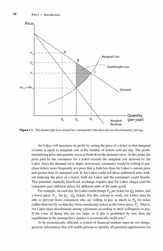
Air Luker will maximize its profit by setting the price of a ticket so that marginalrevenue is equal to marginal cost at the number of tickets sold per day. The profit-maximizing price and quantity occur at Point B on the demand curve. At this point, theprice paid by the consumers for a ticket exceeds the marginal cost incurred by AirLuker. Since the demand curve slopes downward, consumers would be willing to pur-chase tickets more frequently at a price that is both less than Air Luker’s current priceand greater than its marginal cost. If Air Luker could sell these additional units with-out reducing the price of a ticket, both Air Luker and the consumers could benefit.This potential, mutually beneficial, exchange requires that Air Luker charge (and theconsumers pay) different prices for different units of the same good.

For example, on each day Air Luker could charge PB per ticket for QB tickets, anda lower price, PC, for QC�QB tickets. For this scheme to work, Air Luker must beable to prevent those consumers who are willing to pay as much as PB for ticket(rather than not fly on that day) from purchasing tickets at the lower price, PC. That is,Air Luker must discriminate among consumers according to their willingness to pay.If the costs of doing this are too large, or if this is prohibited by law, then theequilibrium in the monopolist’s market is economically inefficient.5

To be economically efficient, a system of financial markets must do two things:generate information that will enable persons to identify all potential opportunities for


Figure 1.1. The deadweight loss created by a monopolist who does not use discriminatory pricing.

mutually beneficial intertemporal exchanges, and provide mechanisms through whichpersons can make these exchanges. To a considerable extent, financial marketsaccomplish both tasks by organizing trading in financial securities. There are, how-ever, situations in which financial markets fail to create an efficient allocation ofresources. Economists call these situations market failures.

Definition of a Failure of a Financial MarketA failure of a financial market is an allocation of resources in which thereare opportunities for mutually beneficial intertemporal exchanges that arenot undertaken.

1.6 Examples of Market Failures

There are three kinds of market failures that occur in the intertemporal allocation ofresources: the problem of agency, the problem of asymmetric information, and theproblem of asset substitution. We describe these problems briefly here. In chapter 13,we analyze these failures in detail and examine some of the ways that firms andinvestors use to mitigate them.

1.6.1 The Problem of Agency

An agency is a relationship in which one person, called the agent, manages the interestsof a second person, called the principal. Ideally, the agent subordinates his or her owninterests completely to the interests of the principal. The problem of agency is that if theinterests of the agent are not fully compatible with those of the principal, and if the prin-cipal cannot costlessly monitor the actions of the agent, the agent might pursue his or herown interests to the detriment of the principal. The extent to which the principal suffersdue to a problem of agency varies directly with the cost that the principal would incur tomonitor the agent perfectly.

The problem of agency arises in a firm that is operated by a small number of pro-fessional managers who act as agents for a large number of diverse shareholders, noneof whom owns a large proportion of the shares. It would be prohibitively costly for theshareholders to monitor perfectly the performance of their managers. First, the man-agers have superior access to relevant information. Second, it is difficult to organize alarge number of diverse shareholders to act as a cohesive unit on every question.Third, the smaller the proportion of the firm that a shareholder owns, the smaller is thecost that he or she would be willing to incur for the purpose of monitoring the man-agers more closely.

An obvious example of the problem of agency is that managers might use someof the shareholders’ resources to purchase excessively luxurious offices, membershipsin clubs, travel on the firm’s aircraft, and other perquisites rather than investing theseresources in projects that will generate wealth for the shareholders.

A less obvious example of a problem of agency occurs because the managers aremore willing to accept a lower expected return on the firm’s investments in exchangefor a lower level of risk than the shareholders would prefer to do. This problem arisesif a significant proportion of the managers’ future wealth depends on their reputations


as managers. These reputations would be diminished were the firm to producemediocre results, let alone fail. Shareholders can reduce the risk of mediocre earningsin any one firm by holding a diversified portfolio of investments in several firms.6

Clearly, managers cannot reduce the risk to their reputations by working simultane-ously for many firms. Since the shareholders can use diversification to reduce therisks of mediocre earnings in a single firm, the shareholders are more willing to havetheir firm undertake risky projects that have higher expected returns than theirmanagers’ less risky, reputation-preserving projects.

1.6.2 The Problem of Asymmetric Information

Both parties to a proposed transaction have information (and beliefs) about the possi-ble future outcomes of that transaction. The information is asymmetric if one partyhas material information that the other party does not have. Material information isinformation that a person would pay to acquire before deciding whether to enter a pro-posed transaction. The problem of asymmetric information is that the inability of aparty that possesses material information to transmit that information credibly to asecond party can prevent what would otherwise be a mutually beneficial exchange.

An example of the problem of asymmetric information occurs if a firm lackssufficient cash to finance a profitable new project. To raise cash for the project, the firmoffers to sell newly created shares of stock. To the extent that investors who are notcurrent shareholders purchase the new shares, the current shareholders will cede to thenew shareholders a portion of the ownership of the firm. But the value of the firm willincrease as a consequence of undertaking the new project. Whether the current share-holders gain or lose wealth depends on the amount by which the new project increasesthe value of the firm relative to the proportion of the firm that the new shareholdersacquire.

Prospective new shareholders must decide what proportion of the firm they mustacquire if they are to recover their investment. The larger the amount by which thenew project will increase the value of the firm, the smaller the proportion of the firmthe new investors must acquire. Further, the smaller the proportion of the firm that thenew shareholders acquire, the larger the proportion of the firm that the current share-holders will retain, and the wealthier those current shareholders will be.

There is a conflict of interest between the current shareholders and the prospec-tive new shareholders. If the firm’s managers act in the interests of the current share-holders, the managers have an incentive to overstate the value of the new project so asto induce the prospective new shareholders to finance the project in exchangefor acquiring a small proportion of the firm. Knowing the incentives of the managers,the prospective new shareholders might insist on acquiring so large a proportion of thefirm that, even with the new project, the current shareholders will lose wealth to thenew shareholders. If the managers expect that their current shareholders will losewealth as a consequence of financing the project by issuing new shares, the managerswill forego the project. Foregoing the profitable project is economically inefficient.By definition, a profitable project will generate sufficient earnings to allow the newshareholders who financed the project to recover their investment and to create aprofit that can be shared by the current and the new shareholders.


A profitable project provides the potential for a mutually beneficial exchange. Torealize the potential, the parties to the exchange must agree on terms that will bemutually beneficial. In the example described above, if the managers cannot crediblyinform the prospective new shareholders about the value of the project, the currentshareholders, acting through their managers, will be unable to effect a mutually bene-ficial exchange with the prospective new shareholders, even though the new projectwould be profitable.

1.6.3 The Problem of Asset Substitution

The problem of asset substitution is the incentive that a firm’s managers have to trans-fer wealth from the firm’s bondholders to its shareholders by substituting riskier proj-ects for less risky ones. In section 1.4.3 of this chapter, we examined a simple modelin which investors who differ in their willingness to tolerate uncertainty could effect amutually beneficial exchange by choosing between contractual and residual claims toan uncertain outcome. In that example, there is no risk of default on the contractualclaims because even in a bad year the output of the combined farms is sufficient to paythe contractual claims.

In a more realistic example, the residual claimants would be the shareholders,who would control the firm through their managers. The contractual claimants wouldbe bondholders, who would have no right to participate in the management of the firmunless there is a default on the bonds. The market value of the bonds depends on theprobability that the firm will default.

Suppose that the managers of the firm sell the two farms that comprise the firm,and use the proceeds to invest in a new project that has the same expected payoff asthe former firm but a higher probability of a default on the bonds. For example, the mini-mal and maximal payoffs of the new project might be 400 tons and 3,600 tons of corn,respectively. The average payoff would remain at 2,000 tons ([400 �3600])/2�2000),but there is now a positive probability that the firm will not be able to make the contractual payment of 900 tons to the bondholders.7

The increase (from zero) of the probability of a default on the bonds will reducethe market value of those bonds. Since the average value of the annual payoff to thefirm remains at 2,000 tons of corn, the market value of the entire firm will notchange.8 Since the claims of the bondholders and the claims of shareholders constitutethe entirety of the claims on the firm, the market value of the shareholders’ claim mustincrease.

We conclude that (at least under some conditions) the firm’s managers can trans-fer wealth from the bondholders to the shareholders by substituting a riskier projectfor a less risky one.

Now suppose that a firm attempts to finance a risky new project by selling bonds.Recognizing that the firm’s managers have an incentive to transfer wealth frombondholders to shareholders by substituting a riskier project for the project that thebondholders intended to finance, the bondholders might refuse to purchase the bonds.If the firm has no other way to finance the new project, the opportunity for a mutuallybeneficial exchange (between prospective bondholders and current shareholders) willbe foregone, creating an economic inefficiency.


Nevertheless, financial markets operate within a set of regulations imposed bylaw. One example of these regulations is the set of information that a firm must pro-vide if its securities are to be publicly traded on organized exchanges. A second exam-ple is the regulation of trading on inside information. An important part of theassessment of the performance of financial markets is, therefore, an analysis of theeffect of public policy on the economic efficiency of financial markets.

1.7 Issues in Public Policy

Governments regulate financial markets in many ways. Economists can evaluate eachregulation against the criterion of economic efficiency by determining how that regu-lation is likely to affect the market’s ability to promote mutually beneficial intertem-poral exchanges. Here are a few examples of important questions in the regulation offinancial markets:

1. Should the government regulate the fluctuation of the prices of financial secu-rities? For example, should there be a limit on the amount by which a price canchange during a day (or an hour) before trading in that security is suspended?

2. Should investors be allowed to use borrowed money to finance mergers andacquisitions? Should hostile takeovers be permitted?9 Should firms be allowedto adopt super majority provisions or poison pill provisions as defenses againsttakeovers?10

3. Should persons with inside information be allowed to trade on that information?4. Corporations are allowed to deduct from their taxable income the interest paid

to their bondholders. Should corporations be allowed to deduct dividends also?5. Many firms compensate their senior executives in part by giving them options

to purchase the firm’s stock at a predetermined price. The firms assert that theexistence of these options makes the executive’s interests more compatiblewith the interests of the shareholders, thus mitigating the problem of agency.In what way, if any, should firms be required to include the costs of theseoptions when reporting their earnings?

1.8 The Plan of the Book

The economics of financial markets is a systematic analysis of how these marketsenable consumers to use mutually beneficial intertemporal exchanges as part of theirstrategies to maximize their levels of lifetime utility. A system of financial markets is economically efficient if, in equilibrium, there are no further opportunities forconsumers to increase their levels of lifetime utility by undertaking additionalintertemporal exchanges. We use these concepts of mutually beneficial exchanges andeconomic efficiency to organize our analysis throughout the book.

We begin in part II by considering in greater detail how consumers use financialmarkets to maximize lifetime utility. We first explain how consumers maximize life-time utility when there is no uncertainty about future outcomes of investment projects.


By abstracting from uncertainty, we can establish analytical principles that are analo-gous to principles that hold when future outcomes are uncertain.

In particular, we first present the efficient markets hypothesis in a setting in whichthere is no uncertainty about future payments. This efficient markets hypothesis andthe Modigliani-Miller theorem are seminal concepts that have guided much of theresearch, both theoretical and empirical, in the economics of financial markets. Theefficient markets hypothesis states that the current prices of securities reflect all that iscurrently known about the future payments that the owners of these securities willreceive. The Modigliani-Miller theorem asserts some relationships between a firm’schoice of investment projects and its choice of how to finance them. We conclude partII (in chapter 6) with an elementary consideration of some of the issues that arisewhen consumers face uncertainty about future payments.

To analyze intertemporal allocation when future payments are uncertain, wemust explain the determinants of the prices of financial securities. To do this, we willrequire some concepts from probability and statistics. We develop these concepts inpart III for students who have no knowledge in this area. Students who have an ele-mentary familiarity of probability and statistics can easily skip part III. In part IV, wedevelop the fundamental capital asset pricing model. Although this model does notenjoy the empirical success that economists once thought that it would have, it is theintellectual forebear of current theoretical and empirical models of security prices.We present these recent models, and a brief review of their empirical records, inchapter 10.

In part V, we consider two empirical areas of financial economics. We begin bypresenting in chapter 11 a detailed discussion of the efficient markets hypothesis whenfuture payments are uncertain. In chapter 12, we explain the empirical method ofevent studies that economists use to quantify the effects of isolated pieces of informa-tion on the value of a firm’s securities. Economists also use event studies to testvarious implications of the efficient markets hypothesis.

In part VI, we examine several ways in which financial markets increase the levelof economic efficiency. We discuss the optimal capital structure of a firm in chapter13. The capital structure is the organization of the claims that investors have on thefirm’s earnings. We saw in the present chapter that investors can construct mutuallybeneficial exchanges by organizing these claims into contractual claims and residualclaims. The Modigliani-Miller theorem and the literature that has followed it haveenriched our understanding of how a firm’s choice of its capital structure can promotemutually beneficial exchanges that would otherwise be foregone. In particular, weexplain how the optimal choice of capital structure can mitigate the negative effects ofasymmetric information, problems of agency, and problems of asset substitution oneconomic efficiency.

In the remainder of part VI, we examine how insider trading (chapter 14), options(chapter 15), and futures contracts (chapter 16) can affect the level of economicefficiency.

In part VII, we present in chapter 17 a brief survey of topics that we do notaddress in this book. To include these topics would make the book rather long for anintroductory treatment of the economics of financial markets. Some of the topicswould be difficult to analyze adequately in an introductory textbook.


We conclude in chapter 18 by restating and consolidating, in the context ofeconomic efficiency, the analyses of the earlier chapters.

Problems

1. Mr. Block’s potato farm produces between 500 and 800 tons of potatoes eachyear if there is bad weather, and between 700 and 1,000 tons each year if there is goodweather. The farm has several investors who together own a bond that entitles them toreceive 600 tons of potatoes each year. Today there is .5 probability that weather willbe good next year. If tomorrow that probability is changed to .4 for the succeedingyear, what will happen to the price for which the investors could sell their bond?

2. ABC Furniture has been struggling to get customers into its store. In anattempt to increase sales, the firm has advertised that interest-free payments on furni-ture are not due until one year after the furniture is purchased. Under what conditionwould this be a mutually beneficial exchange between ABC Furniture and prospectivenew customers?

3. Mr. Brown wants to increase his current consumption by $100. The currentinterest rate paid by a bank for deposits is 10%, and the bank is willing to lend at 15%.If Mr. Brown can guarantee that he will repay a loan that he might obtain fromMr. Green, is it economically efficient for Mr. Green to keep $100 in the bank?

4. Ms. White and Ms. Black own farms next to each other. When the weather isgood, each farm produces 2,000 tons of apples per year. When the weather is bad,each farm produces 1,000 tons per year. Ms. White is risk-averse. Ms. Black is willingto accept additional risk in exchange for a sufficient increase in her average rate ofreturn. If good and bad weather occur with equal probability, and if Ms. White willaccept a guaranteed return of 1,000 apples per year, can the two women effect a mutu-ally beneficial exchange? What type of claim would each woman hold?

Notes

1. An intertemporal exchange is one in which the two sides of the exchange occur at differenttimes. For example, Person A will give something of value to Person B at time 0 in exchange fora commitment by Person B to give something of value to Person A at a later time. In some cases,Person B will promise to deliver things of value at several future times. An essential property ofan intertemporal exchange is the risk that Person B will be unable to make the promised delivery,or will refuse to do so. Another form of risk arises if what Person B promises to deliver dependson an outcome (such as the size of a crop) that will not be known until some future time.

2. Inventories of unsold consumption goods accumulated in the production sector increasethe feasible levels of future consumption beyond what these levels would otherwise be.Therefore, these inventories are capital goods.

3. In more sophisticated models, the quantity of tickets that Air Luker could sell per day at a given price would be uncertain. In these models, the quantities on the horizontal axis would be the average (or expected) numbers of tickets sold per day at various prices. There is no


assumption that consumers are identical in their willingness to pay for tickets. Among thoseconsumers who purchase tickets for a given day when the price is PA, there could be some con-sumers who would have paid more than PA for a ticket rather than not flying on that day. Theheight of the demand curve at Point A is the maximal price that Air Luker can charge per ticketand sell QA tickets per day. Equivalently, if Air Luker were to increase the price above PA, someconsumers would fly less frequently, with the result that Air Luker would sell fewer than QAtickets per day.

4. A more sophisticated analysis would recognize that the heights of the marginal revenueand the marginal cost curves at the quantity QA are the instantaneous rates at which total rev-enue and total cost would change in response to a change in quantity starting from QA.

5. The technical term for the value of the mutually beneficial exchanges foregone is dead-weight loss. Most introductory texts in microeconomics explain how imperfect competition (ofwhich a monopoly is only one example) creates deadweight losses. Some texts explain howfirms and consumers can reduce deadweight losses by using devices such as discriminatorypricing. In chapter 13, we explain how firms can reduce deadweight losses by choosing thekinds of securities to issue.

6. To reduce her risk, the investor must diversify her portfolio across firms whose earningsare not highly correlated. We shall examine the question of optional diversification for aninvestor in chapters 8 (on portfolio theory) and 9 (on the capital asset pricing model).

7. If the firm has accumulated some reserves of corn, it could pay the bondholders even inbad years, but a sufficiently long consecutive run of bad years would exhaust the firm’sreserves, producing a default.

8. The conclusion requires an assumption that investors are risk neutral.9. A hostile takeover is an event in which a group of investors attempts to gain control of a

firm against the opposition of the firm’s current management. The means of gaining control isto acquire a sufficient number of the firm’s shares to elect directors who will replace the currentmanagers (and their policies) with a new set of managers (and policies).

10. A supermajority provision is a provision in a firm’s corporate charter that requiresapproval of more than 50% of the directors or the shareholders before certain kinds of changescan be undertaken. A poison pill is a provision that would transfer wealth from new sharehold-ers to the firm’s current shareholders if the new shareholders acquire enough shares to dismissthe current management.



In chapter 1, we explained that the essential function of a system of financial marketsis to facilitate mutually beneficial intertemporal exchanges. We also learned thateconomists use the concept of economic efficiency to evaluate how well financialmarkets, as regulated by public policy, perform. In this chapter, we discuss therelationship between financial markets and economic efficiency. Financial marketsfacilitate mutually beneficial intertemporal exchanges by organizing trading in finan-cial securities. These securities, and the information contained in their prices, enableindividuals to reach higher levels of lifetime utility than would be possible in theabsence of financial markets. We begin this chapter with a brief treatment of financialsecurities, followed by a discussion of the more important tasks that financial marketsmust perform to be economically efficient. We include brief treatments of two kindsof market failures. We conclude with a general discussion of informational efficiencyand the efficient markets hypothesis.

2.1 Financial Securities

A financial security is a saleable right to receive a sequence of future payments. Thesize of each future payment can be either guaranteed or determined by the outcome ofsome uncertain future event. The number of payments in the sequence can be finite, orthe sequence can continue indefinitely into the future. Here are five examples,presented in order of increasing complexity:

Definition of a BondA bond is a saleable right to receive a finite sequence of guaranteed payments.

For example, a bond could be a saleable right to receive $100 on the last businessday of March, June, September, and December, beginning in March 2002 and endingin December 2010, plus a single payment of $10,000 on the last business day in 2010.This bond would be analogous to a bank account from which a person intends to with-draw $100 each calendar quarter during the years 2002 through 2010, with a finalwithdrawal of $10,000 at the end of 2010 that will reduce the balance in the account to zero.

That the bond is saleable means that an investor who purchases the bond whenthe firm issues it early in 2002 does not have to hold the bond until 2010, when the

2 Financial Markets and EconomicEfficiency

19

firm makes the final payment required by the bond. In other words, any time beforethe end of 2010, the investor can sell the bond to another investor. The second investorpurchases from the first investor the right to receive the payments that remain in thesequence. Of course, the price that the second investor will pay depends on how manypayments remain in the sequence, and on the second investor’s alternative opportuni-ties for investment. The fact that the bond is saleable to other investors makes it moreattractive to any investor.

A bond is a contract between a borrower and a lender. The borrower could be a sin-gle person or a firm. Similarly, the lender could be a single person or a financial institu-tion such as a bank, an insurance company, or a pension fund. The borrower is theissuer of the bond; the lender is the owner of the bond. The contract that defines the bond requires the issuer of the bond to make a specified sequence of payments tothe owner of the bond, and to do things that protect the bond’s owner against the possi-bility that the issuer might not make the promised payments on time. Typically, theborrower issues the bond to obtain funds to finance the purchase of an asset as aninvestment. For example, a railroad might issue a bond to purchase a set of newlocomotives. To protect the interests of the lender, the borrower might be required tomaintain insurance on the locomotives, and to allow only engineers certified by theFederal Railroad Administration to operate those locomotives.

By the definition of a bond, the obligations of the issuer of the bond to whoeverowns the bond at the moment are guaranteed. But what is the nature of the guarantee?What recourse is available to the owner of the bond should the issuer fail to meet hisor her obligations, for example, by failing to make the promised payments on time, orby failing to carry the required amount of insurance?

The legal term for a failure to meet one’s contractual obligations specified by abond is default.1 If the issuer creates a default, the present owner of the bond acquiresspecified rights to the assets of the issuer. For example, should a railroad fail to makethe required payments to the owner of the bond, that owner might acquire the right toask a court to seize the locomotives, sell them, and use the proceeds to make therequired payments to the owner of the bond.

The saleability of bonds enables investors to create mutually beneficialexchanges. Consider the following example of a bond issued by a person to financethe purchase of a house.

Homeowners frequently finance the purchase of a home by borrowing moneyfrom a bank. To induce the bank to make the loan, the homeowner issues a bond to thebank. The bond requires the issuer (the homeowner) to make a specified sequence ofpayments to the owner of the bond (the bank) and to do various things to protect thebank’s interest, such as carrying fire insurance, paying the property taxes, and main-taining the home in good repair. The homeowner guarantees performance of theseobligations by giving a mortgage to the bank. The mortgage is a lien on the propertythat entitles the bank to seize the property and sell it should the homeowner create adefault.2

Banks that purchase bonds issued by homeowners usually sell those bonds toother investors, who form a pool of these bonds. These investors then issue securitiesthat are saleable rights to the sequences of payments that the homeowners have prom-ised to make. These securities are called mortgage-backed securities. Although the


homeowners will make the payments directly to the banks that originated the loans,the banks will pass those payments to the investors who purchased the mortgagedloans, and those investors will, in turn, pass the payments to the persons who pur-chased the mortgage-backed securities. This process of creating mortgaged-backedsecurities is an example of a set of mutually beneficial exchanges. The banks special-ize in originating loans, rather than purchasing rights to receive sequences of pay-ments. The investors who purchase the loans from the banks specialize in creatingdiversified pools of loans, and thus reducing the risks borne by the persons whopurchase the securities that are backed by this pool of loans.

The issuer of the bond borrows money by selling the bond to an investor, whothereby becomes a lender. The price that the investor will pay for the bond determinesthe cost that the investor pays for obtaining the loan. For example, suppose that a rail-road wants to borrow $11,000,000 to purchase a locomotive. The railroad offers to sell10 bonds at a price of $1,100,000 each. Each bond is a promise to pay $1,400,000 peryear for 10 years. Over the 10 years, the investors will receive a total of $14,000,000as a return on their investment of $11,000,000.

The railroad’s attempt to raise $11,000,000 by selling 10 bonds for $1,100,000each might not succeed. If investors believe that the railroad might be late with someof the promised payments, or might be unable to complete the payments, the investorsmight be willing to pay only $1,000,000 for each of the bonds. In this event, the rail-road would have to sell 11 bonds (at $1,000,000 each) to raise the $11,000,000required to purchase the locomotive. Over the term of the loan, the railroad wouldhave to pay to the bondholders $1,400,000 on each of 11 bonds. The total that the rail-road would repay for the loan of $11,000,000 would be (11 bonds)($1,400,000 perbond)�$15,400,000. When the railroad must sell 11 bonds to raise the $11,000,000 topurchase the locomotive, the investors who finance that purchase obtain a return of$15,400,000 on their investment of $11,000,000. The railroad must pay an additional$1,400,000 ($15,400,000�$14,000,000) to finance the locomotive because investorsperceive a higher risk of late or missing payments.3

Since a bond is a saleable right to receive a sequence of payments, any investorcan become a lender in due course by purchasing the bond from a previous owner.Consequently, the investor who became a lender by purchasing the bond from theissuer need not remain a lender until the issuer makes the final payment required bythe bond. At any time while the issuer is paying off the loan, the original lender canrecover at least a portion of the unpaid balance of the loan by selling the bond toanother investor.4

Definition of Common StockA share of common stock is a saleable right to receive an indefinitely longsequence of future payments, with the size of each payment contingent onboth the firm’s future earnings and on the firm’s future opportunities tofinance new investment projects. These payments to the stockholders arecalled dividends.

Typically, a firm will pay a dividend on its common stock at regular intervals,such as semiannually or quarterly. Shortly before each date on which a dividend is

Chapter 2 ■ Financial Markets and Economic Efficiency 21

scheduled, the firm’s directors announce the size of the forthcoming dividend. Thedirectors are free to choose whatever size of dividend they believe is in the longer-term interests of the investors who own the common stock.5 The directors might retainsome of the firm’s earnings for use in financing future investment projects. In particu-lar, the directors can decide to pay no dividend.

Unlike a bond, a share of common stock is not a contractual right to receivea sequence of payments. The owners of the common stock are the owners of the firm.As owners, the (common)6 shareholders elect persons to the board of directors and thereby control the firm. The directors determine the size and the timing of thedividend payments. In particular, the directors can use some or all of the firm’s earn-ings to finance new projects, rather than paying those earnings to the shareholders asdividends.

Payments to bondholders and shareholders depend on the firm’s ability to gener-ate earnings. As explained above, the bondholders have a contractual claim on thoseearnings. By contrast, the shareholders have a residual claim on the earnings. Thedirectors may pay to the shareholders whatever earnings remain after the bondholdersare paid, although the directors may retain some or all of those residual earnings tofinance new projects.

Firms issue common stock to raise money to finance projects. Unlike the case ofa bond, the investors who purchase newly issued shares of common stock from a firmdo not have the right to get their money back at the end of some specified number ofperiods. These investors can, however, in effect withdraw their money by selling theirshares to other investors, just as investors who own bonds can withdraw their moneyprematurely by selling bonds to another investor. Of course, the ability of an investorto withdraw money by selling a security depends on the current price of that security.That current price depends on all investors’ current expectations of the ability of thefirm to generate earnings over the future.

If common stocks were not saleable rights, firms would have difficulty financingnew projects by selling common stock. To understand the economic significance ofthe saleability of rights, consider the decision to construct a new home. A house pro-vides a stream of services over time. These services occur as protection from the ele-ments, a commodious place in which to raise a family and to enjoy one’s friends andrelatives, and a safe place to store important possessions. It is difficult to construct ahome that is both comfortable and that will not outlast the time when the owner eitherwants to move elsewhere (e.g., for retirement) or dies. Few persons would construct acomfortable home designed to last many decades if they did not have the right to sellor to rent that home to another person at any time in the future. The right to sell thehome provides people who finance the construction with the ability to “disinvest”should they want to reallocate their resources in the future. It would be economicallyinefficient to prohibit transfers of ownership of existing homes. If such a prohibitionwere in effect, there would be far fewer homes built, and those that were built wouldbe less comfortable and less durable. Moreover, the incentive to preserve the homesthrough timely maintenance would be diminished.

The same arguments apply to expensive and durable capital goods, such as arailway line. The investors who finance the construction of the line by purchasingsecurities from the railroad acquire a right to receive dividends based on the future


earnings generated by the line. But few persons would purchase the new securitieswithout the right to disinvest in the future by selling the securities to other investors.

Definition of a Callable BondA callable bond is a bond that the issuing firm has the right to cancel by paying to the bond’s current owner a fixed price that is specified in the definition of that bond.

A firm might want to issue a callable bond to provide a quick way to refinance its debt should interest rates fall. Of course, the same callability that provides anadvantage to the firm that issued the bond creates a disadvantage to an investor whoholds that bond. Should the firm call the bond when interest rates fall, the owner of thebond will receive cash. With interests now lower, the former owner of the bond willhave to accept a lower rate of return when he or she reinvests that cash. Therefore, toinduce investors to hold callable bonds, the issuing firms will usually have to provide some incentive, such as setting the levels of the promised payments higherthan they would be on a bond that is identical in all other respects, but that is notcallable.

Consider the bond described at the beginning of this section. That bond requiresthe issuing firm to pay $100 to whoever owns the bond when a payment is due. Thepayments continue quarterly through the end of 2010. At that time, the firm makes afinal payment of $10,000. In effect, the firm has borrowed $10,000 until the end of2010. Until that time, the firm will pay interest at an annual rate of 4% ($400 per year/$10,000�4% per year).7

Now suppose that interest rates fall. A bank will now lend $10,000 to the firm atonly 2% per year. Suppose that the bond on which the firm is now paying $400 peryear is callable at $10,050; that is, the firm can cancel the bond at any time by paying$10,050 to whoever owns the bond at that time. The amount of money that the firmmust pay in order to cancel the bond is the call price of the bond. A simple calculationwill show that the firm can improve its position by borrowing the call price of $10,050from the bank, at 2%, and using that money to call the bond away from its currentowner. In effect, the firm pays $50 for the opportunity to refinance the $10,000 loan at2% rather than at 4%.

A loan that is secured by a mortgage on a residence is analogous to a callablecorporate bond. To borrow from a bank, the homeowner sells a bond to the bank. Thebond requires the homeowner to make regular payments to the bank. To guaranteethe payments, the homeowner gives the bank a mortgage, which entitles the bank toacquire title to the house should the homeowner fail to make the required paymentson time.8 In most cases, the seller of the bond (the homeowner) has the right to can-cel the bond at any time, without notice or penalty, by paying the balance due on theloan (including accrued interest, if any). The bond is thus callable by the homeowner,and the call price is the current outstanding balance on the loan. In the late 1990s andearly 2000s, many homeowners refinanced their mortgaged loans as interest ratesfell. In doing so, the homeowners called their existing bonds by paying off thebalances of the loans, then issued new bonds (i.e., took out new mortgaged loans) atlower interest rates.


Knowing that the mortgaged loans were callable, the banks might have insistedon an offsetting advantage, such as higher interest rates on the initial loan, or a largerdown payment (which would reduce the homeowner’s incentive to create a default).

Definition of a Convertible BondA convertible bond is a bond that provides its owner an option to convert thebond into a fixed number of shares of the firm’s common stock at a fixedprice. The firm that issued the bond must accept the conversion by eitherissuing new stock to the converting bondholder, or by purchasing shares ofits own stock in the market and delivering them to the converting bondholder.

Sometimes a firm lacks sufficient funds to finance a profitable investment proj-ect. In many of these cases, it is possible to construct a mutually beneficial exchangebetween the firm’s current shareholders and new investors who could finance the proj-ect by purchasing new securities issued by the firm. The problem is that the prospec-tive new investors fear that the firm’s managers will use their superior information tooffer the new securities only under conditions that will transfer wealth from the newinvestors to the current shareholders. That is, while the new project offers a potentialfor a mutually beneficial exchange, the possibility that the managers might exploittheir superior information to the detriment of the new investors prevents the old share-holders and the new investors from realizing this potential for mutual gain. By defini-tion, this inability to realize a potential for a mutually beneficial exchange is anexample of economic inefficiency.

Under some conditions, current shareholders and new investors can eliminate theinefficiency created by the managers’ superior information by selling bonds that are bothcallable and convertible. One of the required conditions is that, to protect themselvesagainst losing wealth to the firm’s current shareholders, the prospective new investorswill finance the project only by purchasing bonds rather than purchasing newly issuedshares of stock. Bondholders have more protection in the event that the proposed projectfails to generate the levels of earnings anticipated by the firm’s managers.

A second condition is that the managers of the firm must incur sufficiently largecosts to their reputations as managers if the firm were to default on the bonds. Mostinvestment projects have some probability of failing to generate sufficient earnings toenable the firm to make the promised payments on the bonds. If the firm has no bondsoutstanding, there can be no default, because there are no contractual claims.Therefore, for any given probability of default, the higher the reputational cost to themanagers of a default, the stronger is their incentive to induce the bondholders to con-vert their contractual claims (the bonds) to residual claims (shares of stock). If theprice at which the firm can call the bonds is sufficiently low, and if the proportion ofthe ownership of the firm that the converting bondholders can acquire by convertingtheir bonds to stock is sufficiently high, the managers can induce the bondholders toconvert once the project gets underway and begins to show promise, but no guarantee,that there will be no default.

In summary, when managers have superior information about a potentially prof-itable new project, prospective investors might be willing to finance the project onlyby purchasing bonds. Managers, however, because of concern about the damage totheir reputations, might be willing to have the firm finance the project only by selling


newly created shares of stock. Neither bonds nor stock will enable the potential newinvestors and the firm’s current shareholders to effect a mutually beneficial exchange.Under some conditions, issuing a callable, convertible bond, which is a hybrid of abond and common stock, will enable the firm to effect the mutually beneficialexchange that would otherwise be foregone. We discuss this phenomenon in detail inchapter 13.

The last example of a financial security that we offer here is a call option.

Definition of a Call OptionA call option is the right, but not the obligation, to purchase a specific secu-rity at a fixed price by paying an exercise price prior to a fixed date.

Suppose that a call option on IBM common stock has an exercise price equal to$90. The expiration date is September 30, 2007. Investors who own this option have aright, but not an obligation, to purchase 100 shares of IBM common stock on or beforeSeptember 30, 2007, by paying $90 per share. If they fail to do so by that time, theoption will expire.

If the price of IBM is, for example, $98 when an investor exercises his option, hewill obtain a profit from the exercise equal to $800. This is so because he can immedi-ately resell for $98 each of the 100 shares that he will have purchased for $90. Ofcourse, if the price of IBM is less than the $90 exercise price of the option, theinvestor who owns the option will not exercise it. He would incur a loss by doing so.

Options are contracts created by private investors. For example, Mr. Green offersa contract under which he promises to deliver 100 shares of IBM common stock, andaccept in payment $90 per share, if the investor who owns the contract calls upon himto do so on or before September 30, 2007. Mr. Green sells this contract to an investorat a price determined in a competitive market. The price of the option, which is calledthe premium, fluctuates over the life of the option according to investors’ beliefs aboutthe future values of IBM common stock relative to the fixed exercise price of $90. Themore strongly persuaded investors are that the price of IBM will rise (or rise further)above $90, the greater is the price that investors will be willing to pay for an option topurchase IBM shares at a price of only $90. Similarly, if the price of IBM is currentlyless than $90, and investors have little reason to believe that the price will rise above$90 before September 30, 2007, the price of the option will be low.

The investor who created the option, Mr. Green, keeps the premium for which heinitially sold the option. This is his profit if the option is never exercised.

Options are complex financial securities that enable investors to create mutu-ally beneficial exchanges that would otherwise be too costly to conduct. Some ofthese exchanges involve the reallocation of risk in ways that are analogous to, but more complex than, the example that we described for Ms. Tall and Ms. Short insection 1.3.3 of chapter 1. An extension of the theory of options, called real options,provides a better understanding of how a firm should decide which investment proj-ects to undertake when the future returns to those projects are uncertain. We presenta further description of options in chapter 15. We also examine the economic func-tion of options there.

We conclude this subsection by asserting that financial markets organize tradingin a large variety of securities. Each kind of security exists only because investors find


that security useful for reducing the costs of creating intertemporal exchanges at dif-ferent times and under different market conditions. As we stated earlier in this section,some potentially beneficial exchanges will not be realized unless investors can tradethese securities, or use the information contained in their prices to infer characteristicsof the sequences of future payments associated with those securities.

2.2 Transaction Costs

An important way in which financial markets assist individuals in making intertempo-ral exchanges is to reduce transaction costs. The term transaction costs is broadlydefined to include all those costs that individuals incur to make exchanges. Two indi-viduals can make a mutually beneficial exchange only if they have different prefer-ences (such as willingness to tolerate uncertainty). But these individuals must firstfind each other, and then they must agree on the terms of the exchange. As stated ear-lier, these terms can be quite complex if the exchange is an intertemporal one.Consider, for example, the complexity of the terms in a callable, convertible bond.

Financial markets reduce these costs by providing easy access to a central locationat which individuals can trade standardized securities. Financial securities are usuallytraded on exchanges. Common stocks, for example, are traded on the New York StockExchange, the American Stock Exchange, and on an informal but highly integratedorganization of dealers called the over-the-counter market. Bonds are traded through aset of independent and competing dealers. This informal network of dealers is knownas the over-the-counter exchange. Options are traded on many organized exchanges,including the American Stock Exchange, the Boston Options Exchange, and theChicago Board Options Exchange.

Some securities require one or both parties to an exchange to purchase or sellsome other security, or some commodity, on a future date. Associated with theexchanges on which these securities are traded are clearinghouses which guaranteethat the investors who trade in these securities will meet their obligations. By insuringindividual investors against the risk of default by other investors, the clearinghousesincrease the attractiveness of these securities as the basis for mutually beneficialexchanges.

2.3 Liquidity

The liquidity of an asset is a measure of the increase in the cost that one would incuras a consequence of increasing either the size of a transaction in that asset or the speedat which the investor wants to conclude the transaction. A highly liquid asset is one forwhich the price at which the asset can be bought or sold is little affected by increasesin the speed or the size of the transaction. Some examples will help.

A house is a relatively illiquid asset: its price depends on the speed with which theseller or the buyer wants to conclude the sale. Houses are not standardized. A realtor


might advise a homeowner that she can expect to sell her house for a price between$115,000 and $120,000 if she sets an asking price of $124,900 and if she is willing towait for several weeks while prospective buyers canvass the market, inspect her home,obtain an engineer’s report on the house, arrange for financing, and have their attorneysinspect the title to the property. She could probably sell her house more quickly, butonly if she accepts a price that is low enough to induce a prospective buyer to foregocollecting the information that would reduce the risks involved in purchasing her home.One could probably sell his home within a day, for cash, by accepting a price that is20% of what realtors estimate that the owner could get if he were willing to leave thehouse on the market for several weeks. In fact, if the owner were willing to accept asufficiently low price, a realtor would probably purchase the home immediately, forcash, and then put it on the market for resale.

Similarly, if a person insists on purchasing a home immediately, he or she canusually do so by offering to pay sufficiently more than the asking price, in cash, andforegoing the customary protections, such as an engineer’s report.

Unlike a house, the shares of IBM common stock are quite liquid. The prices atwhich an investor can buy or sell a share of IBM stock do not depend on the speed ofthe transaction. One reason for this is that shares of IBM common stock are standard-ized. Any share is a perfect substitute for any other share, just as any five-dollar bill isinterchangeable with any other five-dollar bill. No one is interested in inspecting aparticular share of IBM as a condition of purchasing it. Second, shares of IBM com-mon stock are actively traded on the New York Stock Exchange. During the hours thatthe market is open for trading,9 dealers in IBM common stock, called specialists,announce a bid price at which they will purchase shares of IBM into their inventory,and an asked price at which they will sell shares of IBM out of their inventory. Thedealers may change these prices at any time to reflect changes in the interest thatinvestors have in IBM shares.

Suppose that a dealer’s bid price is $80.25, and that his asked price is $80.75.10 Inthis case, an investor can immediately sell a share of IBM for $80.25, or purchase ashare of IBM for $80.75. But what would happen if the investor wants to purchase orsell 800,000 shares immediately? The dealer is not obligated to guarantee his pricesfor any quantity. An attempt to purchase a large number of shares immediately wouldprobably drive the dealer’s prices up. Similarly, an attempt to sell a large number ofshares immediately would drive the dealer’s prices down.

A dealer in any good provides a service of predictable immediacy by enablingpersons to buy or sell that good without notice.11 To provide this service, the dealermust maintain a stock of the good in question and a stock of money (or access tocredit). Dealers in IBM stock on an organized exchange are no exception. If theirinventories of IBM stock are depleted, they must replenish them or risk being unableto accommodate investors who wish to purchase shares of IBM immediately. Dealerscan replenish their inventories of IBM stock by simultaneously raising their bid andasked prices. Raising the bid price will induce some investors to sell larger quan-tities of IBM shares to a dealer, or sell given quantities sooner, than these investorswould otherwise do. Similarly, raising the asked price will induce investors whowould otherwise purchase shares of IBM from the dealer to do so in smaller quantitiesor at lower speeds.


We conclude that small quantities of IBM common stock are highly liquid: theprice of the asset will not be affected by the speed at which the transaction is con-ducted. But as the size of the transaction increases, the liquidity of the asset decreases.

Finally, consider a checking account in a bank. This account is defined in terms ofdollars. A typical depositor can, without notice to the bank, redeem any part of the bal-ance, or all of it, for cash. Compare this to a certificate of deposit at a bank. A certifi-cate of deposit is an agreement by which a bank will pay a fixed rate of interest to adepositor who intends to leave a fixed amount of money on deposit for a fixed amountof time. In most cases, the depositor may withdraw the deposit (liquidate the certifi-cate) only by forfeiting a portion of the interest that has accrued. Thus, certificates ofdeposit pay higher rates of interest than do checking accounts (many of which pay nointerest), but certificates of deposit are less liquid.

There are two reasons why liquidity matters. One reason is that intertemporalexchanges involve claims on future payoffs, and the future is uncertain. The secondreason is that some investment projects require large infusions of resources at the out-set, and thereafter generate very long sequences of relatively small payments. Themore liquidity financial markets provide, the larger the set of mutually beneficialintertemporal exchanges that individuals can conduct. Therefore, greater liquidity infinancial securities increases the opportunities for individuals to increase their levelsof lifetime utility.

Here is an example. The Mosquito Point Barge Company wants to purchase anew tugboat. With the new tugboat, the company can offer faster and more reliableservice, and thus (it hopes) obtain higher profits. But the company does not have suf-ficient funds of its own to purchase the new tugboat.

Mr. Apple is willing to finance the Mosquito Point Barge Company’s investmentproject by reducing his current consumption below his current income. He will obtaina financial security, which is a saleable claim on the uncertain sequence of futurepayoffs that the project will generate. But there is another source of uncertainty.Mr. Apple has aging parents. They might be able to care for themselves in their ownhome until they die, but they might not. Thus, Mr. Apple might want to purchase full-time care for them, and on relatively short notice. The more liquid the financialsecurity offered by the barge company, the lower the cost that Mr. Apple will incur ifhe decides to sell the security on short notice. Thus, the more liquid the security, themore easily the barge company can finance its project. But any investment projectinvolves an intertemporal exchange. We conclude that liquidity promotes intertempo-ral exchanges, and thus enables individuals to increase their levels of lifetime utility.

Consider another example. The Spring Lake Railroad wants to build a tunnel. Thetunnel will enable the railroad to move freight trains more quickly between two majorcities and thus generate a relatively small increase in profit each year. The tunnel willbe extremely expensive to build, but it will last indefinitely with little maintenance.The railroad cannot finance the construction of the tunnel with its own funds.

No investor plans to live long enough to justify helping to finance the tunnel inexchange for a right to receive an indefinitely long sequence of relatively small pay-ments. But if the investors can obtain financial securities, each investor can hold thesecurity for some number of years, then sell it to a younger investor. The older


investor will sell to the younger investor the right to receive the remaining paymentsthat the tunnel will generate. By purchasing the security, the younger investorenables the older investor, in effect, to withdraw her investment. As with the bargecompany, the more liquid the security offered by the railroad, the greater the extent towhich individuals can increase their levels of lifetime utility by making intertempo-ral exchanges.

2.4 The Problem of Asymmetric Information

There is an asymmetry of information in a proposed exchange if one of the personshas better information than the other person about the likely outcome of theexchange. If the person with the superior information could credibly reveal the infor-mation to the other person, the two persons could create a mutually beneficialexchange. But if the person with the superior information cannot credibly reveal thatinformation, a potential mutually beneficial exchange will be foregone and, therefore,there will be an inefficient allocation of resources. This inefficiency arises notbecause the outcome of the proposed exchange is uncertain. It is relatively easy fortwo persons to create a mutually beneficial exchange that involves claims to an uncer-tain outcome if both parties to the exchange are equally informed about the probabil-ities of the possible outcomes. Rather, it is the asymmetry of information that canprevent what, under symmetric information, would have been a mutually beneficialexchange.

Asymmetric information is a significant problem for firms. The managers of afirm will often have superior information relative to investors about the uncertain out-comes of a proposed investment project. If the firm does not have sufficient internalfunds to finance the project, the managers will have to raise funds externally by offer-ing new securities to investors. Asymmetric information between the managers andthe prospective new investors may prevent the managers from raising funds on termsthat will prevent a transfer of wealth from the firm’s current shareholders to the newinvestors. Consequently, the firm will choose to forego an investment project thatcould increase the wealth of both the current shareholders and the new investors.Therefore, there will be an inefficient allocation of resources.

The seminal contribution to the problem of asymmetric information is the paperby George Akerlof titled “The Market for ‘Lemons’: Quality, Uncertainty, and theMarket Mechanism.”12 In 2001, Akerlof was awarded a Nobel Prize in economics for his work on asymmetric information. Akerlof’s work has generated a large litera-ture. He analyzes a market for used automobiles to show how asymmetric informationbetween buyers and sellers can cause the market to collapse, with the result thatopportunities for mutually beneficial exchanges are foregone; as a result of this collapse, the market fails. In the next subsection, we present a simple version ofAkerlof’s model and then apply this model to the case of a firm developed in anotherseminal paper by Stewart C. Myers and Nicholas Majluf, “Corporate Financing andInvestment Decisions When Firms Have Information That Investors Do Not.”13


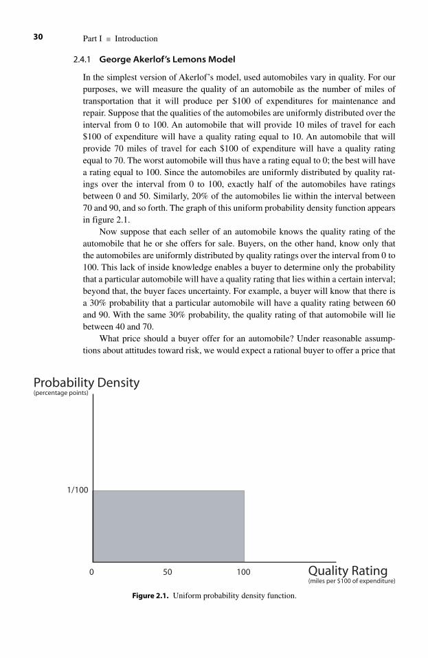
2.4.1 George Akerlof’s Lemons Model

In the simplest version of Akerlof’s model, used automobiles vary in quality. For ourpurposes, we will measure the quality of an automobile as the number of miles oftransportation that it will produce per $100 of expenditures for maintenance andrepair. Suppose that the qualities of the automobiles are uniformly distributed over theinterval from 0 to 100. An automobile that will provide 10 miles of travel for each$100 of expenditure will have a quality rating equal to 10. An automobile that willprovide 70 miles of travel for each $100 of expenditure will have a quality ratingequal to 70. The worst automobile will thus have a rating equal to 0; the best will havea rating equal to 100. Since the automobiles are uniformly distributed by quality rat-ings over the interval from 0 to 100, exactly half of the automobiles have ratingsbetween 0 and 50. Similarly, 20% of the automobiles lie within the interval between70 and 90, and so forth. The graph of this uniform probability density function appearsin figure 2.1.

Now suppose that each seller of an automobile knows the quality rating of theautomobile that he or she offers for sale. Buyers, on the other hand, know only that the automobiles are uniformly distributed by quality ratings over the interval from 0 to100. This lack of inside knowledge enables a buyer to determine only the probabilitythat a particular automobile will have a quality rating that lies within a certain interval;beyond that, the buyer faces uncertainty. For example, a buyer will know that there isa 30% probability that a particular automobile will have a quality rating between 60and 90. With the same 30% probability, the quality rating of that automobile will liebetween 40 and 70.

What price should a buyer offer for an automobile? Under reasonable assump-tions about attitudes toward risk, we would expect a rational buyer to offer a price that


0 50 100

1/100

Probability Density(percentage points)

Quality Rating(miles per $100 of expenditure)

Figure 2.1. Uniform probability density function.

is compatible with the average quality of the automobiles that are for sale. For exam-ple, suppose that the buyer is a taxicab company that purchases large numbers of usedautomobiles each year. If the quality ratings of the used automobiles offered for saleare uniformly distributed from 0 to 100, this company can expect that the averagequality of the automobiles that it purchases each year will be equal to 50. Therefore,the price that the company will offer for any particular automobile will be based onthe assumption that the quality of that automobile will be equal to 50.

Now consider the sellers of these used automobiles. Each seller knows the qualityrating of each of his automobiles. Suppose that Mr. Black knows that the quality ratingof his automobile is 75. Unless he can certify this quality to prospective buyers, he willhave to accept a price based on a quality rating of only 50. The alternative is to with-draw his offer to sell the automobile. The same situation faces half of the prospectivesellers, who know that the quality ratings of their automobiles exceed 50. In Akerlof’smodel, half of the prospective sellers will therefore withdraw from the market becausethey know that the market will underprice their automobiles. Consequently, the auto-mobiles offered for sale have quality ratings that range from 0 to only 50. Although theprospective buyers cannot determine the quality of any particular automobile, they doknow the distribution of quality ratings. Therefore, the buyers can anticipate that theaverage quality rating of the automobiles offered for sale will be equal to 25, not 50.

Buyers will then revise the price that they are willing to pay downward to a valuethat is compatible with a quality rating of 25. This downward revision of the buyers’prices will cause the sellers to withdraw those automobiles that have quality ratingsbetween 25 and 50, and the price that buyers will offer will decrease further. Thisprocess is degenerative. In the limit, the market collapses because no seller can expectto obtain a fair price for an automobile.

In Akerlof’s model, the market fails because there are potential mutually benefi-cial exchanges that are not realized. The failure of the market occurs because there isasymmetric information between buyers and sellers, and the sellers have no way totransmit their information credibly to the buyers.

Consider again Mr. Black, whose automobile has a quality rating of 75. Supposethat Mr. Black has a strong preference for new automobiles. Specifically, he is willingto sell his current automobile for a price that would be appropriate for a quality ratingof 65, so that he could apply the proceeds of that sale toward the purchase of a newautomobile. Ms. Green, on the other hand, would be willing to pay more than whatMr. Black is willing to accept if she can be certain that the quality rating of his auto-mobile is 75. If Mr. Black could credibly transmit his information to Ms. Green, theycould conclude a mutually beneficial exchange. But in the absence of a way to elimi-nate the asymmetry of the information, the potential for mutual gain will be foregone,and thus the market will fail. Only by eliminating the effects of the asymmetric infor-mation will the market be able to promote an efficient allocation of resources.

2.4.2 A Simple Example of Asymmetric Information and Economic Inefficiency for a Firm

We present a simple example of how asymmetric information between a firm andprospective new investors can create an inefficient allocation of resources. Assume first


that the only kind of security that a firm can issue is common stock. Firms haveprospective profitable projects but lack sufficient internal funds with which to financethem. Being profitable,14 the new projects could provide a mutually beneficial exchangebetween new investors, who would finance the projects by purchasing newly createdshares of common stock, and the firms’ current shareholders. Before the firm sellsnewly created shares, the current shareholders own 100% of the firm.

By purchasing newly created shares, the new investors provide additional resourcesto the firm. In exchange, the new investors acquire a portion of the ownership of thefirm from the current shareholders. Whether the new investors gain or lose wealthdepends on (1) the value of the resources that the new investors transfer to the firm bypurchasing the new shares, (2) the amount by which the value of the firm will increaseonce the new project is undertaken, and (3) the proportion of the ownership of the firmtransferred from the current shareholders to the new investors. The prospective newinvestors have reason to fear that firms will exploit their superior information so thatthe combined effect of factors (1), (2), and (3) will transfer wealth from the newinvestors to the current shareholders, thus imposing a net loss on the new investors.Consequently, the prospective new investors will not purchase the new shares,the firms cannot undertake the projects, and the profit that could have been shared bythe new investors and the current shareholders is foregone. Since potential mutuallybeneficial exchanges are foregone, resources are allocated inefficiently; there is adeadweight loss.

Consider another example. There is a large number of firms in the economy, halfof which are strong firms and half of which are weak firms. Each firm will survive forexactly one more year, after which it will be rendered worthless. During that finalyear, each strong firm will generate earnings equal to $150 from its regular operations.Each weak firm will generate only $50 from its regular operations.

Each strong firm and each weak firm has an opportunity to invest in a new proj-ect that will increase that firm’s earnings for its final year. The cost of the new project is $100 for each firm. A strong firm can use the new project to increase itsearnings by $120. A weak firm can generate only $110 in additional earnings from theproject. The management of each firm knows whether that firm is strong or weak. Noone else can discover whether a particular firm is strong or weak until the end of thefinal year. Assume that the bank’s interest rate is zero.15 Since the project costs only$100, every firm has an incentive to undertake the project. Alas, each firm has paidout in dividends to its shareholders all of its earnings from previous years; conse-quently, no firm has any idle cash with which to finance new projects.

Because no firm has idle cash, a firm must sell new shares of stock to raise the$100 required to start the project. If a firm sells new shares and undertakes the project, two things will occur. First, the value of the firm will increase because the project is profitable. Second, once the new shares are issued, the proportion of thefirm owned by the current shareholders will decrease by the proportion of the firm thatthe new shareholders acquire. The new shareholders will own a proportion of theentire firm, including the new project. Their claim is not limited to the earnings of thatproject. If the proportion of the firm acquired by the new shareholders is too largerelative to the value of the new project, the current shareholders will lose wealth as aconsequence of financing the project by issuing new shares.


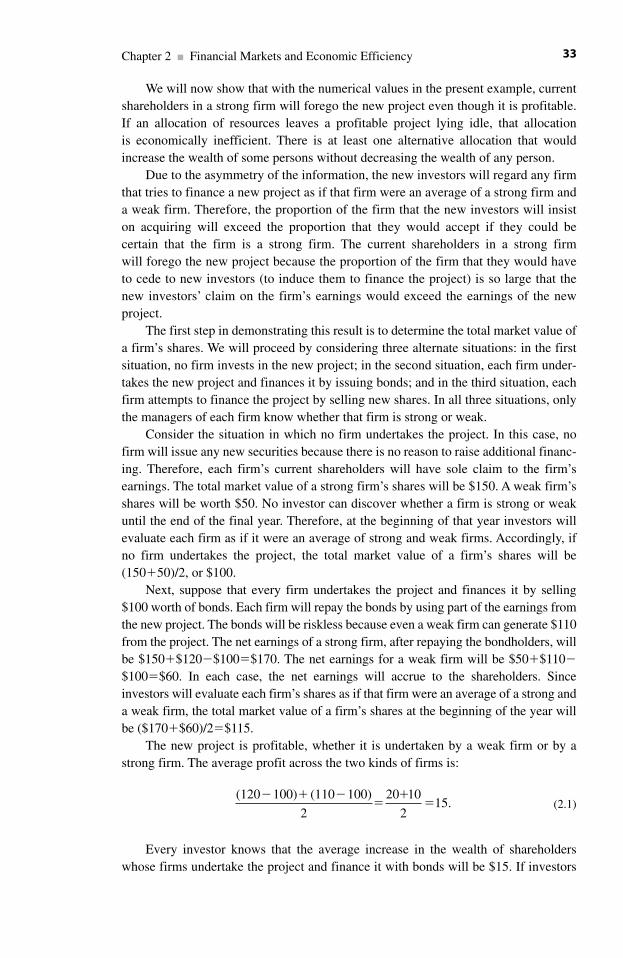
We will now show that with the numerical values in the present example, currentshareholders in a strong firm will forego the new project even though it is profitable.If an allocation of resources leaves a profitable project lying idle, that allocation is economically inefficient. There is at least one alternative allocation that wouldincrease the wealth of some persons without decreasing the wealth of any person.

Due to the asymmetry of the information, the new investors will regard any firm that tries to finance a new project as if that firm were an average of a strong firm anda weak firm. Therefore, the proportion of the firm that the new investors will insiston acquiring will exceed the proportion that they would accept if they could be certain that the firm is a strong firm. The current shareholders in a strong firm will forego the new project because the proportion of the firm that they would haveto cede to new investors (to induce them to finance the project) is so large that thenew investors’ claim on the firm’s earnings would exceed the earnings of the newproject.

The first step in demonstrating this result is to determine the total market value ofa firm’s shares. We will proceed by considering three alternate situations: in the firstsituation, no firm invests in the new project; in the second situation, each firm under-takes the new project and finances it by issuing bonds; and in the third situation, eachfirm attempts to finance the project by selling new shares. In all three situations, onlythe managers of each firm know whether that firm is strong or weak.

Consider the situation in which no firm undertakes the project. In this case, nofirm will issue any new securities because there is no reason to raise additional financ-ing. Therefore, each firm’s current shareholders will have sole claim to the firm’searnings. The total market value of a strong firm’s shares will be $150. A weak firm’sshares will be worth $50. No investor can discover whether a firm is strong or weakuntil the end of the final year. Therefore, at the beginning of that year investors willevaluate each firm as if it were an average of strong and weak firms. Accordingly, ifno firm undertakes the project, the total market value of a firm’s shares will be(150�50)/2, or $100.

Next, suppose that every firm undertakes the project and finances it by selling$100 worth of bonds. Each firm will repay the bonds by using part of the earnings fromthe new project. The bonds will be riskless because even a weak firm can generate $110from the project. The net earnings of a strong firm, after repaying the bondholders, willbe $150�$120�$100�$170. The net earnings for a weak firm will be $50�$110�

$100�$60. In each case, the net earnings will accrue to the shareholders. Sinceinvestors will evaluate each firm’s shares as if that firm were an average of a strong anda weak firm, the total market value of a firm’s shares at the beginning of the year willbe ($170�$60)/2�$115.

The new project is profitable, whether it is undertaken by a weak firm or by astrong firm. The average profit across the two kinds of firms is:

(2.1)

Every investor knows that the average increase in the wealth of shareholderswhose firms undertake the project and finance it with bonds will be $15. If investors

(120 100) (110 100)

2

20 10

215.

� � ��

��


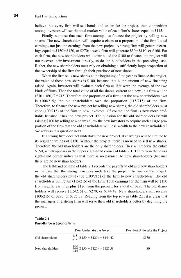
believe that every firm will sell bonds and undertake the project, then competitionamong investors will set the total market value of each firm’s shares equal to $115.

Finally, suppose that each firm attempts to finance the project by selling newshares. The new shareholders will acquire a claim to a proportion of the firm’s totalearnings, not just the earnings from the new project. A strong firm will generate earn-ings equal to $150�$120, or $270; a weak firm will generate $50�$110, or $160. Foreach firm, the new shareholders who contributed the $100 to finance the project willnot recover their investment directly, as do the bondholders in the preceding case.Rather, the new shareholders must rely on obtaining a sufficiently large proportion ofthe ownership of the firm through their purchase of new shares.

When the firm sells new shares at the beginning of the year to finance the project,the value of those new shares is $100, because that is the amount of new financingraised. Again, investors will evaluate each firm as if it were the average of the twokinds of firms. Then the total value of all the shares, current and new, in a firm will be(270�160)/2�215. Therefore, the proportion of a firm that the new shareholders ownis (100/215); the old shareholders own the proportion (115/215) of the firm.Therefore, to finance the new project by selling new shares, the old shareholders mustcede (100/215) of the firm to new investors. Of course, the firm is now more prof-itable because it has the new project. The question for the old shareholders is: willraising $100 by selling new shares allow the new investors to acquire such a large pro-portion of the firm that the old shareholders will lose wealth to the new shareholders?We address this question next.

If a strong firm does not undertake the new project, its earnings will be limited toits regular earnings of $150. Without the project, there is no need to sell new shares.Therefore, the old shareholders are the only shareholders. They will receive the entire$150, which appears in the upper right-hand corner of table 2.1. The zero in the lowerright-hand corner indicates that there is no payment to new shareholders (becausethere are no new shareholders).

The left-hand column of table 2.1 records the payoffs to old and new shareholdersin the case that the strong firm does undertake the project. To finance the project, the old shareholders must cede (100/215) of the firm to new shareholders. The oldshareholders will retain (115/215) of the firm. Total earnings for the firm will be $150from regular earnings plus $120 from the project, for a total of $270. The old share-holders will receive (115/215) of $270, or $144.42. New shareholders will receive(100/215) of $270, or $125.58. Reading from the top row in table 2.1, it is clear thatthe managers of a strong firm will serve their old shareholders better by declining theproject.


Table 2.1Payoffs for a Strong Firm

Does Undertake the Project Does Not Undertake the Project

Old shareholders ($150 � $120) � $144.42 $150

New shareholders ($150 � $120) � $125.58 $0100–––215

115––––215

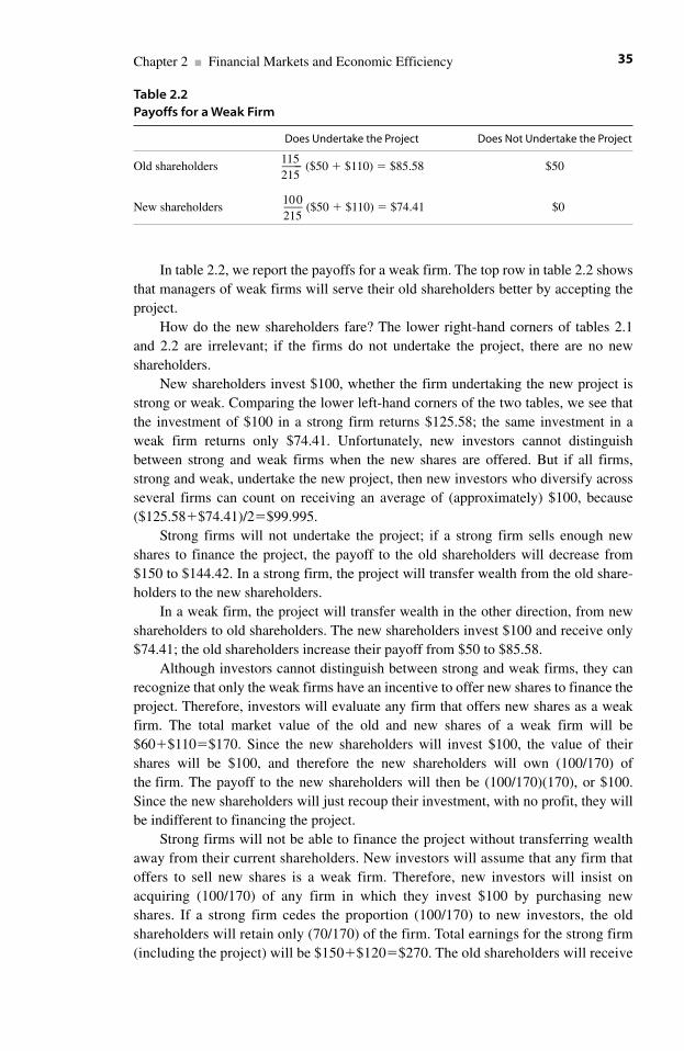
In table 2.2, we report the payoffs for a weak firm. The top row in table 2.2 showsthat managers of weak firms will serve their old shareholders better by accepting theproject.

How do the new shareholders fare? The lower right-hand corners of tables 2.1and 2.2 are irrelevant; if the firms do not undertake the project, there are no new shareholders.

New shareholders invest $100, whether the firm undertaking the new project isstrong or weak. Comparing the lower left-hand corners of the two tables, we see thatthe investment of $100 in a strong firm returns $125.58; the same investment in aweak firm returns only $74.41. Unfortunately, new investors cannot distinguishbetween strong and weak firms when the new shares are offered. But if all firms,strong and weak, undertake the new project, then new investors who diversify acrossseveral firms can count on receiving an average of (approximately) $100, because($125.58�$74.41)/2�$99.995.

Strong firms will not undertake the project; if a strong firm sells enough newshares to finance the project, the payoff to the old shareholders will decrease from$150 to $144.42. In a strong firm, the project will transfer wealth from the old share-holders to the new shareholders.

In a weak firm, the project will transfer wealth in the other direction, from newshareholders to old shareholders. The new shareholders invest $100 and receive only$74.41; the old shareholders increase their payoff from $50 to $85.58.

Although investors cannot distinguish between strong and weak firms, they canrecognize that only the weak firms have an incentive to offer new shares to finance theproject. Therefore, investors will evaluate any firm that offers new shares as a weakfirm. The total market value of the old and new shares of a weak firm will be$60�$110�$170. Since the new shareholders will invest $100, the value of theirshares will be $100, and therefore the new shareholders will own (100/170) ofthe firm. The payoff to the new shareholders will then be (100/170)(170), or $100.Since the new shareholders will just recoup their investment, with no profit, they willbe indifferent to financing the project.

Strong firms will not be able to finance the project without transferring wealthaway from their current shareholders. New investors will assume that any firm thatoffers to sell new shares is a weak firm. Therefore, new investors will insist onacquiring (100/170) of any firm in which they invest $100 by purchasing newshares. If a strong firm cedes the proportion (100/170) to new investors, the oldshareholders will retain only (70/170) of the firm. Total earnings for the strong firm(including the project) will be $150�$120�$270. The old shareholders will receive


Table 2.2Payoffs for a Weak Firm

Does Undertake the Project Does Not Undertake the Project

Old shareholders ($50 � $110) � $85.58 $50

New shareholders ($50 � $110) � $74.41 $0100–––215

115––––215

(70/170)($270) � (.41)($270) � $110.70, which is less than the $150 they will getif their firm declines the project.

We have now established that resources can be allocated inefficiently if there isasymmetric information between managers of firms and shareholders (both currentand prospective). Strong firms cannot credibly identify themselves as strong firms toprospective investors. Consequently, projects that would return $120 (in a strong firm)for an investment of only $100 are foregone.

It is easy to show that a strong firm could increase profits for both old and newshareholders if the firm could communicate credibly with prospective investors,thereby eliminating the asymmetric information. Without the new project, the oldshareholders will receive 100% of $150. Let Z be the proportion of the firm that the oldshareholders will retain after the firm raises $100 by selling new shares. Total earningsfor a strong firm with the project will be $270. Consequently, the old shareholders willgain wealth even though new shareholders are present if Z($270)�$150, or

(2.2)

If old shareholders retain the proportion Z of the firm, then new shareholders willacquire the proportion 1– Z. Since the new shareholders will have invested $100, theywill gain wealth if

We conclude that the managers of a strong firm can create a mutually beneficialexchange between old and new shareholders if the old shareholders retain more than55.6%, but not more than 63%, of the firm.

2.5 The Problem of Agency

In the preceding section on asymmetric information, the market failed to realize somemutually beneficial exchanges because of an inability of some persons to transmitinformation credibly to other persons. If the firm’s investors and its managers were thesame persons, this asymmetry would not arise. In this section, we briefly consider asecond problem that arises from the separation of investors and managers. This is theproblem of agency.

Agency is a relationship between two persons, or groups of persons. One person,called the principal, provides the resources for an enterprise and employs a secondperson, called the agent, to operate the enterprise. The principal not only determinesbroad policies for the agent to follow but also allows the agent some flexibility inadministering these policies. The problem of agency is that the agent might exploit the

(1 Z)($270) $100, or

$270 $100 $270, or

$270 $100

$270or

.63

� �

� �

��

Z

Z,

��Z

Z � �$150$270

.556


(2.3)

flexibility provided by the principal by administering the enterprise so as to favor hisor her own interests rather than those of the principal.

For example, a principal purchases a motel and employs an agent to manage it. Inaddition to renting rooms and collecting revenue, the agent is obligated to find eco-nomical ways to purchase supplies and supervise the staff so as to maintain the repu-tation of the motel as clean, safe, and friendly. The principal allows the agent toilluminate the No Vacancy sign at a “reasonable” time. The principal pays the agent afixed salary that does not depend on the motel’s occupancy rate.

The agent has a conflict of interest with the principal. It is clearly unreasonablefor the principal to expect the agent to remain awake every night until the last room isrented and then work regular hours the next day. Indeed, on some nights the motel willremain below full occupancy throughout the night. On the other hand, few principalswould be satisfied to have the No Vacancy sign illuminated at 5:00 P.M. every day,regardless of how many rooms remain vacant. What will the agent do? What shouldthe principal expect the agent to do? The agent’s behavior will surely affect the princi-pal’s return on investment. It is naive to expect that the agent will resolve in the prin-cipal’s favor every instance in which there is a conflict of interest. This fact will makeany potential rate of return from the motel less attractive. If the problem of agency issufficiently severe, the principal will not invest, with the possibility that some mutu-ally beneficial exchanges will not be realized.

Consider a second example. In this example, the interests of a firm’s managerswill cause them to diversify the firm’s investments across projects to an extent that isnot compatible with the interests of the firm’s shareholders.

Most investors diversify their holdings over several firms’ securities. By doing so,investors can reduce the amplitude of the unpredictable variability of the rate of returnon their invested funds, without reducing the average rate of return on those funds. Thisis possible because it is highly unlikely that every firm’s earnings will increase by thesame percentage or decrease by the same percentage in the same year. A firm’s earningsare subject to two kinds of unpredictable forces. One kind of force affects single firmsor single industries, without affecting the entire economy. An example of this would bea shift of consumers’ preferences away from dining and entertainment outside of thehome, in favor of spending more time in the home. The other kind of force affects allfirms in the economy, but not to the same degree. An example of this would be a deci-sion of the Federal Reserve Board to change interest rates.

Most large firms operate several investment projects simultaneously. Portfoliotheory, which we present in chapter 8, indicates that these firms face a trade-offbetween the average rate of return on their capital and the variability of that rate ofreturn. To a limited extent, a firm can decrease the variability of its rate of return,without decreasing its average rate of return, by choosing projects whose individualrates of return are not highly correlated with each other. But once the firm has chosenprojects that will minimize the variability of its rate of return while producing a givenaverage rate of return, any further decrease in variability requires that the firm accepta reduction in its average rate of return.

The firm’s shareholders and its managers have a conflict of interest with regard tochoosing the combination of the firm’s average rate of return and the volatility of thatrate of return. Managers’ wealth consists of a portfolio of financial securities and the


market value of their reputation as managers. The financial securities can generateincome, either now or when the managers retire. Their reputations will affect theirability to secure another managerial position should they lose their current position ordesire to move elsewhere. The greater the volatility of the firm’s rate of return, thegreater the risk that a manager could lose his or her position. Therefore, the greater theimportance of the manager’s reputation as a component of her wealth, the stronger theincentive to choose investment projects that will reduce the volatility of the firm’s rateof return, even if this will reduce the firm’s average rate of return.

For example, suppose the firm has debt in its capital structure. Debt requires thatthe firm make periodic payments of interest, regardless of whether the firm’s earningsat the time that the interest payments are due are high or low. The greater the volatilityof the firm’s earnings, the greater the risk that the firm will have trouble making theinterest payments. If the firm encounters this kind of difficulty, the manager’sreputation might suffer.

A typical shareholder will not have his or her wealth as heavily concentrated in thefirm as the firm’s managers do, because reputation is not an issue for the shareholder.The shareholder will create an investment portfolio by purchasing the securities ofseveral firms, just as a single firm will operate a portfolio of investment projects.Therefore, the shareholder is in a situation that is analogous, but not identical, to the sit-uation of a single firm. Within limits, the firm can reduce the volatility of its rate ofreturn by diversifying its investments across projects whose rates of return are nothighly correlated. Similarly, shareholders can reduce the volatility of the rate of returnon their portfolios by diversifying their investments across firms whose rates of returnare not highly correlated. Both the firm and the shareholder can reduce the volatilitiesof their rates of return by accepting a decrease in their average rates of return.

Shareholders, however, enjoy a more favorable trade-off between the average rateof return and the volatility of the rate of return than does the firm. By making invest-ments in several firms, shareholders can diversify their portfolios across the aggregateof all the projects undertaken by all of the firms. Since shareholders can diversify overa larger set of projects than any one firm can, they can reduce the volatility of theirrate of return while incurring a smaller sacrifice in the average rate of return than asingle firm can.

Since managers have a higher concentration of wealth, including their reputation,invested in the firm than the typical shareholders do, managers have a stronger incen-tive to reduce the volatility of the firm’s rate of return than its shareholders do.Therefore, managers and shareholders will often have different preferences about theprojects in which the firm should invest.

2.6 Financial Markets and Informational Efficiency

2.6.1 Information and Mutually Beneficial Exchanges

We have seen that the economic function of financial markets is to facilitate mutuallybeneficial intertemporal exchanges. One element of this function is to reduce the costs of learning about opportunities to make these exchanges. Financial markets


reduce these costs by creating a set of equilibrium prices for an extensive variety offinancial securities.

We know that a financial security is a saleable right to receive a sequence of pay-ments. These sequences of payments are the results of intertemporal exchanges. Sincethe exchanges are intertemporal, the payments necessarily involve both waiting andrisk. In equilibrium, the relative prices of these securities enable investors to evaluatethe underlying intertemporal exchanges on the basis of waiting and risk. By extension,individuals can use the prices of existing financial securities to identify opportunitiesfor new mutually beneficial exchanges.

In later chapters, we explain how individuals can use the relative prices of exist-ing securities to identify prospects for new exchanges. For now, however, we willaddress the economic efficiency and the informational content of the prices of finan-cial securities.

Any system of markets can be evaluated by its contribution to economic effi-ciency. We recall that economic efficiency is an allocation of resources in which thereare no further opportunities for mutually beneficial exchanges. Financial markets con-tribute to economic efficiency by creating a set of relative prices for financial securi-ties that contain information about mutually beneficial intertemporal exchanges. Iffinancial markets are to be economically efficient, then the information about thepotential costs and benefits in prospective intertemporal exchanges that is containedin the prices of financial securities must be comprehensive and accurate. That is tosay, the information must be such that there are no potential beneficial exchanges thatare foregone. We say that financial markets are informationally efficient if the infor-mation contained in the prices of securities is comprehensive and accurate in the sensejust described.

2.6.2 The Efficient Markets Hypothesis

Definition of the Efficient Markets HypothesisThe efficient markets hypothesis states that the current price of each finan-cial security accurately reflects all the information that is known today aboutthe sequence of future payments that will accrue to an investor who ownsthat security.

The information includes the distribution of those payments over time, and theamplitude of their unpredictable variability. If the efficient markets hypothesis is true,then each security will be priced so that its expected rate of return will provide aninvestor who holds that security with the equilibrium levels of compensation forwaiting and for bearing risk. There will be no mispriced securities. Consequently, ifthe efficient markets hypothesis holds, it will be impossible for an investor to find asecurity whose rate of return will, on average, outperform the market after allowingfor waiting and for bearing risk.

Consider this simple example of how the efficient markets hypothesis would affectthe price of a security. The Mosquito Point Barge Company has a long record of payingits shareholders an annual dividend equal to $2 per share. Banks pay interest at the rateof 10% per year on deposits. An investor can, therefore, purchase an income equal to


$2 per year by depositing $20 in a bank. One share of common stock in the barge com-pany will also generate an annual income equal to $2 per year. A straightforward appli-cation of opportunity cost then implies that the equilibrium price of a share in theMosquito Point Barge Company will be $20. Since the two assets generate identicalincomes, the prices of the assets must be equal.

Now suppose that the Mosquito Point Barge Company has unexpectedly receiveda contract with the Weedsport Fertilizer Plant that will enable the barge company toincrease its annual dividend to shareholders from $2 to $3, beginning two years fromnow. Once the company begins paying dividends at the rate of $3 per year, the price ofa share of its common stock will be equal to $30, because an investor would have tomaintain in a bank a deposit equal to $30 to generate an annual income of $3.Although the higher dividend will appear two years from now, the information that thedividend will increase is available now. The efficient markets hypothesis requires thatthe price of a share in the barge company begin to increase immediately to reflect theinformation that the dividend will increase from $2 to $3 two years from now. Theprice of the share will not increase immediately from $20 all the way to $30 becausethe higher dividend rate will not appear immediately. Instead, the price will increasesteadily from $20 to $30 during the time remaining until the new dividend comes intoeffect.

In the preceding example, the information about the new contract with the fertil-izer company appeared all at once, not in small bits over time. Under the efficientmarkets hypothesis, investors must have been surprised by this information. Hadinvestors anticipated the information, the price of the barge company’s common stockwould already have reflected the increase in future dividends.

Consider a second example of how the efficient markets hypothesis would affectthe price of a security. Investors in the Mosquito Point Barge Company will recognizethat the company’s ability to pay dividends will depend on its ability to maintain con-tracts with its current customers and win new customers. Changes in taxes on profitsand in the price of fuel will also affect the company’s ability to pay dividends. Underthe efficient markets hypothesis, the price of a share of common stock in the MosquitoPoint Barge Company will reflect at each moment all the information then knownabout what might happen to future dividends. For example, suppose that the SpringLake Railroad is competing with the barge company for the business of shipping fer-tilizer. If the efficient markets hypothesis holds, then the price of the barge company’scommon stock will change to reflect changes in the probabilities that the railroad willwin the contract to ship the fertilizer.

2.6.3 The Joint Hypothesis

The efficient markets hypothesis states that the current prices of financial securitiesare such that the expected rate of return on each security will provide the equilibriumlevel of compensation for the waiting and the risk that an investor who holds thatsecurity must bear. This means that any empirical test of the efficient markets hypoth-esis is conditional on a second hypothesis that specifies the equilibrium relationshipamong expected rates of return, waiting, and levels of risk. Further, this secondhypothesis must specify how we are to quantify these risks.


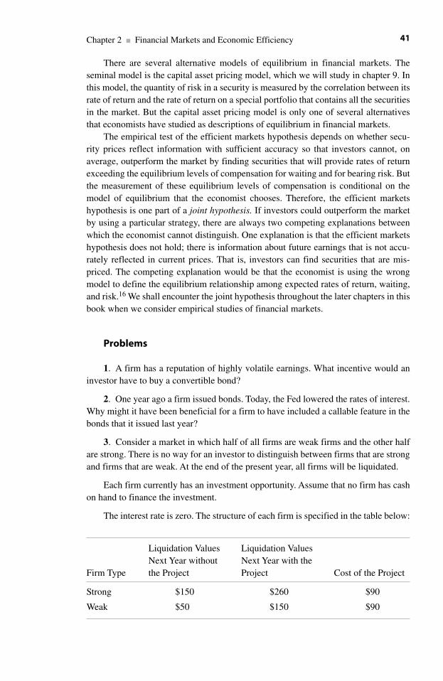
There are several alternative models of equilibrium in financial markets. Theseminal model is the capital asset pricing model, which we will study in chapter 9. Inthis model, the quantity of risk in a security is measured by the correlation between itsrate of return and the rate of return on a special portfolio that contains all the securitiesin the market. But the capital asset pricing model is only one of several alternativesthat economists have studied as descriptions of equilibrium in financial markets.

The empirical test of the efficient markets hypothesis depends on whether secu-rity prices reflect information with sufficient accuracy so that investors cannot, onaverage, outperform the market by finding securities that will provide rates of returnexceeding the equilibrium levels of compensation for waiting and for bearing risk. Butthe measurement of these equilibrium levels of compensation is conditional on themodel of equilibrium that the economist chooses. Therefore, the efficient marketshypothesis is one part of a joint hypothesis. If investors could outperform the marketby using a particular strategy, there are always two competing explanations betweenwhich the economist cannot distinguish. One explanation is that the efficient marketshypothesis does not hold; there is information about future earnings that is not accu-rately reflected in current prices. That is, investors can find securities that are mis-priced. The competing explanation would be that the economist is using the wrongmodel to define the equilibrium relationship among expected rates of return, waiting,and risk.16 We shall encounter the joint hypothesis throughout the later chapters in thisbook when we consider empirical studies of financial markets.

Problems

1. A firm has a reputation of highly volatile earnings. What incentive would aninvestor have to buy a convertible bond?

2. One year ago a firm issued bonds. Today, the Fed lowered the rates of interest.Why might it have been beneficial for a firm to have included a callable feature in thebonds that it issued last year?

3. Consider a market in which half of all firms are weak firms and the other halfare strong. There is no way for an investor to distinguish between firms that are strongand firms that are weak. At the end of the present year, all firms will be liquidated.

Each firm currently has an investment opportunity. Assume that no firm has cashon hand to finance the investment.

The interest rate is zero. The structure of each firm is specified in the table below:


Liquidation Values Liquidation Values Next Year without Next Year with the

Firm Type the Project Project Cost of the Project

Strong $150 $260 $90

Weak $50 $150 $90

A. If each firm finances the project by selling bonds, determine for each firm theincrease in its shareholders’ wealth, and the total market value of the firm’sshares.

B. If each firm could finance the project by issuing additional shares, which typeof firm would undertake the project?

C. How could an investor use a firm’s financing strategy to determine if that firmis strong or weak?

Notes

1. If the issuer of a bond creates a default, that issuer is said to be in default (of his obligationsunder the bond).

2. The term mortgage is commonly used, incorrectly, as a synonym for a loan to purchase ahouse. In fact, the mortgage is not the loan; the mortgage is a lien issued to the bank by thehomeowner on the property as a means of guaranteeing that the homeowner will meet the obli-gations specified by the bond. A loan secured by a mortgage is a mortgaged loan.

3. The additional $1,400,000 is only a potential adjustment for the increase in risk. Should therailroad miss any of the promised payments, the investors would not receive the full$1,400,000. Should the railroad be late with any payments, the investors would lose the interestthat they could have earned by depositing the payments in a bank, had the payments been madeon time.

We conclude that the price that the railroad will have to pay to finance a locomotive willdepend on the risks perceived by the investors to whom the railroad would sell the bonds. Thehigher the perceived risks, the more bonds the railroad will have to sell to raise the $11,000,000.Since each bond requires the railroad to repay $1,400,000 over 10 years, an increase in riskraises the cost to the railroad of financing the purchase of the locomotive. For a sufficiently highlevel of risk, purchasing the locomotive will cease to be a profitable investment project.

4. If there has been an increase in the risk perceived by investors generally between the timethat the investor purchased the bond and the time that he wants to sell it, the price that theinvestor will have to accept for the bond might not be high enough to allow him to recover hisinvestment fully.

5. We will see in section 2.5 and in chapter 13 that the inability of the shareholders to moni-tor the directors perfectly creates incentives for the directors to pursue their own interests to thedetriment of the shareholders’ interests. This conflict of interests, and the shareholders’ attemptsto mitigate it, is called the problem of agency.

6. A firm can have two kinds of stock, common and preferred. Owners of preferred stockhave a contractual right to receive a specified sequence of payments subject to the adequacy ofthe firm’s earnings to make those payments after the firm makes the payments promised to itsbondholders. Unlike the bondholders, the owners of the preferred stock have no legal recoursein the event that the firm’s earnings are insufficient to make the promised payments on the pre-ferred shares. Further, the owners of the preferred shares (usually) do not have the right to votefor directors. Thus, bonds, shares of preferred stock, and shares of common stock form a hierar-chy among investors who hold claims to the firm’s earnings. The bondholders have the highestpriority, owners of the preferred shares come next, and owners of the common stock come last.However, as contractual claimants, the owners of the bonds and the preferred stock have an upper limit on the payments that they can receive. As residual claimants, the owners of thecommon stock are entitled to whatever earnings remain after the other two classes of claimants


are paid. Therefore, once the earnings are sufficient to pay the contractual claims, any growth inthe earnings accrues entirely to the owners of the common stock. Since bonds and preferredstock are both forms of a contractual claim, we shall not discuss preferred stock separately.

7. We ignore the effect of quarterly compounding on the calculation of the interest rate.8. The mortgage is not the loan. The mortgage is the lien that the borrower places on the

house to guarantee repayment of the loan.9. Beginning several years ago, investors can also buy and sell many securities from dealers

who operate during hours when the organized exchanges are closed. It is also possible to tradeon foreign exchanges in the securities of American firms.

10. At 12:20 P.M. on June 23, 2004, the bid price for IBM was $90.52, and the asked price was$90.54. The spread between the bid and asked for IBM is low because the volume of trading inthat stock is large.

11. Harold Demsetz introduced the term predictable immediacy in analyzing the economicsof dealers on organized securities exchanges. H. Demsetz, “The Cost of Transacting,” QuarterlyJournal of Economics 82, no. 1 (1968): 33–53.

12. G. A. Akerlof, “The Market for ‘Lemons’: Quality Uncertainty and the Market Mechanism,”Quarterly Journal of Economics 84, no. 3 (1970): 488–500.

13. S. C. Myers and N. Majluf, “Corporate Financing and Investment Decisions When FirmsHave Information That Investors Do Not,” Journal of Financial Economics 13 (1984): 187–221.

14. A profitable project is one that generates future earnings that are sufficiently large, andthat occur sufficiently soon, to provide the investors who finance the project with returns thatexceed what those investors could have obtained by financing alternative projects. The value ofa firm is the amount of money for which a group of investors could purchase the entire firm, andthus obtain exclusive rights to all the firm’s earnings. By undertaking a profitable investment,the firm will increase its value. We discuss the relationship between profitability and value indetail in chapter 3, where we explain the concept of net present value of a sequence of pay-ments.

15. This unrealistic assumption simplifies the arithmetic without affecting the qualitativeeconomic conclusion.

16. There is a third possibility: both the efficient markets hypothesis fails and the economistis using the wrong model of equilibrium.



Part II

Intertemporal Allocation byConsumers and Firms WhenFuture Payments Are Certain


3.1 The Plan of the Chapter

The fundamental economic objective of every person is to allocate her scarce resourcesamong various alternatives so as to maximize her lifetime utility. These alternativesinclude producing goods and services for current consumption, and producing goodsthat can be used as inputs for the production of goods and services in future years. Theallocation of resources each year between these two kinds of production is the essenceof intertemporal allocation.

Even if a person were living on a desert island, without contact with other persons with whom he could cooperate or trade, that person would still have to decidehow to allocate his resources between the production of consumption goods andcapital goods if he wanted to maximize his lifetime utility. A benefit of living in asociety of individuals who cooperate and trade is that each individual can use mutu-ally beneficial exchanges to reach higher levels of lifetime utility than he could reachif he did not cooperate and trade. The function of financial markets is to organizethose intertemporal exchanges.

In this chapter, we develop the fundamental aspects of economics that explain theexistence and operation of financial markets. To focus on the fundamentals, we con-sider a sequence of simple situations. Each situation, although a simplification ofreality, contains the elements of intertemporal allocation. By examining these simplemodels first, we will be able to recognize more easily the fundamental economicaspects in the more complex situations that we address in later chapters.

We first examine a primitive economy in which there is no trading betweenpersons. We then introduce the possibility of trade, but without the convenience ofmarkets. We conclude the chapter by developing the concepts of income, wealth, andpresent values. These concepts are essential to understanding the economics of finan-cial markets.

3.2 A Primitive Economy with No Trading

We can develop the essence of the economics of financial markets by first consideringa primitive society in which individuals produce and consume in isolation from otherconsumers. There are no markets in this society, because there are no exchanges

3 The Fundamental Economics ofIntertemporal Allocation

47

Part II ■ Intertemporal Allocation When Future Payments Are Certain48

among consumers. Each person in this society owns a limited set of resources, whichshe uses to produce goods for her own consumption. These resources consist of the 24hours that she has each day, her ability to work, her levels of various skills, some landthat she cleared in previous years, and a few simple tools that she built in those years.

There are two kinds of goods that she can produce each year. First, she can pro-duce goods, such as food, that she can consume that year. We will call these goods con-sumption goods. Leisure is also a consumption good. She can “produce” leisure simplyby using some of her time to do nothing. Second, she can produce goods this year thatshe can use as factors of production in future years. We will call these goods capitalgoods. Examples of capital goods include tools that will increase her productivity inharvesting food, and ditches to irrigate land and thereby increase its productivity.

In any year, each person’s stock of resources is insufficient to produce all of thegoods that she would like to have. This relative scarcity of resources requires her tomake two kinds of choices each year. First, she must allocate her limited resourcesbetween producing consumption goods and producing capital goods. Second, shemust decide which consumption goods and which capital goods to produce, and inwhat quantities. We assume that her only reason to produce capital goods is toincrease the quantity of consumption goods that she can produce in future years.Therefore, these two kinds of decisions each year will determine the sequence of con-sumption goods that she can enjoy over her lifetime. We assume that she will allocateher scarce resources so as to maximize her lifetime utility.

Students should recall from their introductory course in economics that everychoice involves an opportunity cost. To produce food this year is to forego an oppor-tunity to produce something else this year. Clearly, the production of leisure also hasan opportunity cost.

We are particularly interested in intertemporal opportunity costs. Any unit of con-sumption goods produced this year requires resources that could have been used toproduce capital goods this year. The larger a person’s stock of capital goods, thegreater the volumes of all goods, including consumption goods, that she can producein future years. Therefore, the opportunity cost of any unit of consumption goods pro-duced this year is the increase in the quantities of consumption goods that she willforego in future years as a consequence of not producing capital goods this year. Thisrelationship is reversible. The (intertemporal) opportunity cost of a given increase inthe future production of consumption goods is the quantity of current consumptiongoods that must be foregone in order to release sufficient resources to produce thecapital goods that will be required to produce those future consumption goods.

3.2.1 Stocks, Flows, and Intertemporal Allocation

In economic analysis, it is important to distinguish between mathematical entities thatare measured as stocks and those that are measured as flows. An entity is measured asa stock if its numerical magnitude does not involve the passing of time. An entity ismeasured as a flow if its numerical magnitude is a rate at which the magnitude of astock increases (or decreases) over time.

Consider the following examples. The current balance in your checking accountis measured as a stock; the rate at which you are increasing that balance by making

deposits is measured as a flow. The balance today could be $1,600, and the rate atwhich you are increasing that balance by making deposits could be $300 per month.To say that your balance is $1,600 per day would not make sense; similarly, to say thatyou are making deposits of $300 would be ambiguous without specifying the rate atwhich you are making those deposits. Your balance will grow more rapidly if youmake deposits at the rate of $300 per day, rather than $300 per month.

The unpaid balance on a mortgaged loan is measured as a stock; the rate at whichyou are reducing that balance by making monthly payments is measured as a flow.The national debt is measured as a stock; the national deficit, which is the rate atwhich the debt is increasing per year, is measured as a flow. The value of a person’sinvestment in shares of IBM common stock is measured as a stock; the dividends paidon those shares are measured as a flow.

Capital goods are stocks of resources that are used to produce flows of consump-tion goods. Some capital goods produce consumption goods indirectly by makingother capital goods more productive. For example, an irrigation ditch is a capital goodthat can increase the output of corn per acre of cleared land. The cleared land is also acapital good.

An accumulated stock of consumption goods is a special case of a capital good. Aperson could use a portion of his resources this year to produce food that he thenstores for future consumption. The maximal quantity of corn that a person can con-sume in any year is equal to the sum of what he produces during that year plus thestock of corn that he has accumulated and stored from production in earlier years. Anaccumulated stock of corn increases the quantity of corn that he can consume in agiven year beyond what he produces that year. Therefore, we can regard the accumu-lated (and thus not yet consumed) stock of corn as a capital good.

We conclude that by producing capital goods the person can, in effect, transferresources from the present to the future. The fundamental purpose of financial mar-kets is to enable consumers to create mutually beneficial exchanges that involve theseintertemporal transfers of resources. Therefore, we will be able to appreciate the eco-nomics of financial markets more easily if we pause to consider some of the ways inwhich a consumer can effect these intertemporal transfers even when he produces andconsumes in isolation from other consumers.

3.2.2 Example: Transferring Consumption from the Present to the Future by Storing Current Output

Our first example is transparent. Suppose that Farmer Harold owns 10 acres of tillableland, and suppose that on each acre he can produce either 50 bushels of corn or 25 bushels of oats. Farmer Harold allocates resources between the production of cornand the production of oats for the current year simply by choosing the portions of hisland to use for each crop. The opportunity cost of one bushel of oats is two bushels ofcorn, and the opportunity cost of one bushel of corn is one-half of a bushel of oats.Unless Farmer Harold has chosen to use all of his land to produce oats, he can obtain an additional bushel of oats for consumption this year by reducing his production ofcorn by two bushels. He decides to transfer some land from the production of corn tothe production of oats, and thus he transfers some of his consumption from corn to oats.

Chapter 3 ■ The Fundamental Economics of Intertemporal Allocation 49

Now suppose that Farmer Harold wants to transfer consumption from the currentyear to a future year. Obviously, he cannot transfer land from one year to the next. Landsaved from the production of corn this year is available for the production of oats in thesame year. But Harold cannot save land from one year to the next in the sense that byleaving one of his 10 acres unplanted this year, he will have 11 acres to plant next year.It is impossible to move an acre of land from the present to the future.

But it is possible to accomplish the same effect by storing the output of an acre ofland from one year to the next. If he consumes this year the quantity of oats and cornthat he produces on 9 of his 10 acres, and stores the output that he produces on thetenth acre, then next year he can consume all that he produces on his 10 acres, plus thestored output of 1 acre. In effect, he will have transferred one acre from the present tothe future.

3.2.3 Example: Transferring Consumption from the Present to the Future by Producing Capital Goods

For our second example, we consider a case in which the consumer allocates some ofhis resources this year to produce capital goods. The capital goods will increase theproductivity of her resources in future years.

The quantities of oats and corn that Harold can produce this year depend on howmuch time Farmer Harold allocates to weeding those crops during the growing season.Suppose that he reduces the time that he allocates to weeding and uses that time toimprove the drainage of those acres. This reallocation of his time will increase the pro-ductivity of those acres for future years and decrease the quantities of oats and cornthat he will produce during the current year. Harold will have traded a decrease in hislevel of consumption in the current year for an increase in the levels of consumptionthat his land will support in future years. Therefore, Harold will have transferred con-sumption from the current year to future years.

We have just seen two examples of how a person could transfer consumptionfrom the present to the future. It is also possible to transfer consumption from thefuture to the present.

3.2.4 Example: Transferring Consumption from the Future to the Present by Consuming Capital Goods

Assume that the farmer has allocated some of his resources in previous years toimproving the productivity of those resources. For example, he could have improvedthe drainage of his fields. Similarly, he could have created tools that would improvehis productivity in harvesting, or he could have constructed shelters for storing crops.In each of these three cases, the improvements will require maintenance. Drainageditches will eventually become clogged, tools will become dull or worn out, and shel-ters will require repairs. Assume that these improvements to his resources willincrease their productivity by more than the productivity lost by maintaining them.That is, the improvements provide a net gain in productivity.

The farmer could now transfer some consumption from the future to the present by neglecting the maintenance of the improvements that he created in previous years.


By neglecting maintenance, he can allocate all of his resources to current consumption.In the short run, this will enable the farmer to increase his current level of consumption.Of course in the longer run, the neglect of maintenance will reduce the productivity of his resources, which will reduce the levels at which he can consume in future years.1

3.3 A Primitive Economy with Trading, but with No Markets

We have seen that a person who produces and consumes in isolation from other personscan reallocate consumption between the present and the future. But there are limits tothe ability to do this. In any given year, the person must use some of her resources(which can include previously accumulated stocks of consumption goods) to provideconsumption goods: otherwise she would starve or succumb to the elements. Therefore,she can allocate something less than 100% of her resources to the production of newcapital goods. Similarly, the size of her stock of capital goods limits the extent to whichshe can increase her current consumption by neglecting to maintain those capitalgoods.

In this section, we examine how two or more persons can expand their opportuni-ties to reallocate consumption between the present and the future by trading with eachother.

3.3.1 Trade Based on Comparative Advantage

A fundamental concept in economics is that two persons can both gain by specializingin their production according to the theory of comparative advantage, and then trad-ing.2 Here is a simple example.

Ms. Black and Mr. Green can produce both oats and corn. The production possi-bility frontiers for each person appear in figure 3.1. The combined frontier defines theeconomically efficient combinations of oats and corn that Ms. Black and Mr. Greencan produce jointly if they allocate their resources according to their comparativeadvantages. The vertical intercept of the combined production possibility frontier is at400 units of corn, which is the sum of the maximal amounts of corn that both personscan produce.

We see that Mr. Green is more productive than Ms. Black because his frontier liesfurther from the origin than hers does. The critical difference, however, between thetwo persons is that their frontiers have different slopes.

Now suppose that the two persons want to produce some oats and minimize thequantity of corn foregone by doing so. For every unit of oats that Ms. Black produces,she must forego producing two units of corn. Therefore, her opportunity cost of oneunit of oats is two units of corn. Mr. Green’s farm is different. For every unit of oatsthat he produces, he must forego five units of corn. His opportunity cost of a unit ofoats is five units of corn. In terms of opportunity costs, Ms. Black is more efficient inproducing oats. We say that Ms. Black has a comparative advantage over Mr. Green inproducing oats.


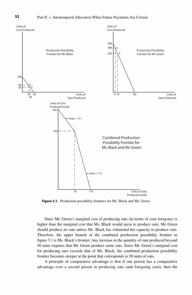
Since Mr. Green’s marginal cost of producing oats (in terms of corn foregone) ishigher than the marginal cost that Ms. Black would incur to produce oats, Mr. Greenshould produce no oats unless Ms. Black has exhausted her capacity to produce oats.Therefore, the upper branch of the combined production possibility frontier in figure 3.1 is Ms. Black’s frontier. Any increase in the quantity of oats produced beyond50 units requires that Mr. Green produce some oats. Since Mr. Green’s marginal costfor producing oats exceeds that of Ms. Black, the combined production possibilityfrontier becomes steeper at the point that corresponds to 50 units of oats.

A principle of comparative advantage is that if one person has a comparativeadvantage over a second person in producing oats (and foregoing corn), then the


100

4020

5040

30 Units ofOats Produced

Units ofCorn Produced

Production PossibilityFrontier for Ms. Black

AA‘

300

280

250

60104 Units ofOats Produced

Units ofCorn Produced

Production PossibilityFrontier for Mr. GreenB

B‘

300

slope = -2:1

slope = -5:1

400

11050 Units of OatsProduced (total)

Units of Corn Produced (total)

Combined Production Possibility Frontier for

Ms. Black and Mr. Green

Figure 3.1. Production possibility frontiers for Ms. Black and Mr. Green.

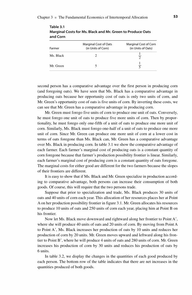
second person has a comparative advantage over the first person in producing corn(and foregoing oats). We have seen that Ms. Black has a comparative advantage inproducing oats because her opportunity cost of oats is only two units of corn, andMr. Green’s opportunity cost of oats is five units of corn. By inverting these costs, wecan see that Mr. Green has a comparative advantage in producing corn.

Mr. Green must forego five units of corn to produce one unit of oats. Conversely,he must forego one unit of oats to produce five more units of corn. Then by propor-tionality, he must forego only one-fifth of a unit of oats to produce one more unit ofcorn. Similarly, Ms. Black must forego one-half of a unit of oats to produce one moreunit of corn. Since Mr. Green can produce one more unit of corn at a lower cost interms of oats foregone than Ms. Black can, Mr. Green has a comparative advantageover Ms. Black in producing corn. In table 3.1 we show the comparative advantage ofeach farmer. Each farmer’s marginal cost of producing oats is a constant quantity ofcorn foregone because that farmer’s production possibility frontier is linear. Similarly,each farmer’s marginal cost of producing corn is a constant quantity of oats foregone.The marginal costs for either good are different for the two farmers because the slopesof their frontiers are different.

It is easy to show that if Ms. Black and Mr. Green specialize in production accord-ing to comparative advantage, both persons can increase their consumption of bothgoods. Of course, this will require that the two persons trade.

Suppose that prior to specialization and trade, Ms. Black produces 30 units ofoats and 40 units of corn each year. This allocation of her resources places her at PointA on her production possibility frontier in figure 3.1. Mr. Green allocates his resourcesto produce 10 units of oats and 250 units of corn each year, placing him at Point B onhis frontier.

Now let Ms. Black move downward and rightward along her frontier to Point A,where she will produce 40 units of oats and 20 units of corn. By moving from Point Ato Point A, Ms. Black increases her production of oats by 10 units and reduces herproduction of corn by 20 units. Mr. Green moves upward and leftward along his fron-tier to Point B, where he will produce 4 units of oats and 280 units of corn. Mr. Greenincreases his production of corn by 30 units and reduces his production of oats by6 units.

In table 3.2, we display the changes in the quantities of each good produced byeach person. The bottom row of the table indicates that there are net increases in thequantities produced of both goods.


Table 3.1Marginal Costs for Ms. Black and Mr. Green to Produce Oatsand Corn

Marginal Cost of Oats Marginal Cost of CornFarmer (in Units of Corn) (in Units of Oats)

Ms. Black 2

Mr. Green 5

12

15

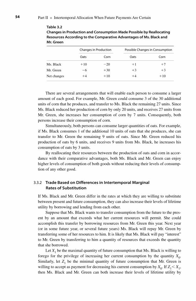
There are several arrangements that will enable each person to consume a largeramount of each good. For example, Mr. Green could consume 3 of the 30 additionalunits of corn that he produces, and transfer to Ms. Black the remaining 27 units. SinceMs. Black reduced her production of corn by only 20 units, and receives 27 units fromMr. Green, she increases her consumption of corn by 7 units. Consequently, bothpersons increase their consumption of corn.

Simultaneously, both persons can consume larger quantities of oats. For example,if Ms. Black consumes 1 of the additional 10 units of oats that she produces, she cantransfer to Mr. Green the remaining 9 units of oats. Since Mr. Green reduced hisproduction of oats by 6 units, and receives 9 units from Ms. Black, he increases hisconsumption of oats by 3 units.

By reallocating their resources between the production of oats and corn in accor-dance with their comparative advantages, both Ms. Black and Mr. Green can enjoyhigher levels of consumption of both goods without reducing their levels of consump-tion of any other good.

3.3.2 Trade Based on Differences in Intertemporal Marginal Rates of Substitution

If Ms. Black and Mr. Green differ in the rates at which they are willing to substitutebetween present and future consumption, they can also increase their levels of lifetimeutility by borrowing and lending from each other.

Suppose that Ms. Black wants to transfer consumption from the future to the pres-ent by an amount that exceeds what her current resources will permit. She couldaccomplish this transfer by borrowing resources from Mr. Green this year. Next year(or in some future year, or several future years) Ms. Black will repay Mr. Green bytransferring some of her resources to him. It is likely that Ms. Black will pay “interest”to Mr. Green by transferring to him a quantity of resources that exceeds the quantitythat she borrowed.

Let X1 be the maximal quantity of future consumption that Ms. Black is willing toforego for the privilege of increasing her current consumption by the quantity X0.Similarly, let Z1 be the minimal quantity of future consumption that Mr. Green iswilling to accept as payment for decreasing his current consumption by X0. If Z1 X1,then Ms. Black and Mr. Green can both increase their levels of lifetime utility by


Table 3.2Changes in Production and Consumption Made Possible by ReallocatingResources According to the Comparative Advantages of Ms. Black and Mr. Green

Changes in Production Possible Changes in Consumption

Oats Corn Oats Corn

Ms. Black �10 �20 �1 �7

Mr. Green �6 �30 �3 �3

Net changes �4 �10 �4 �10

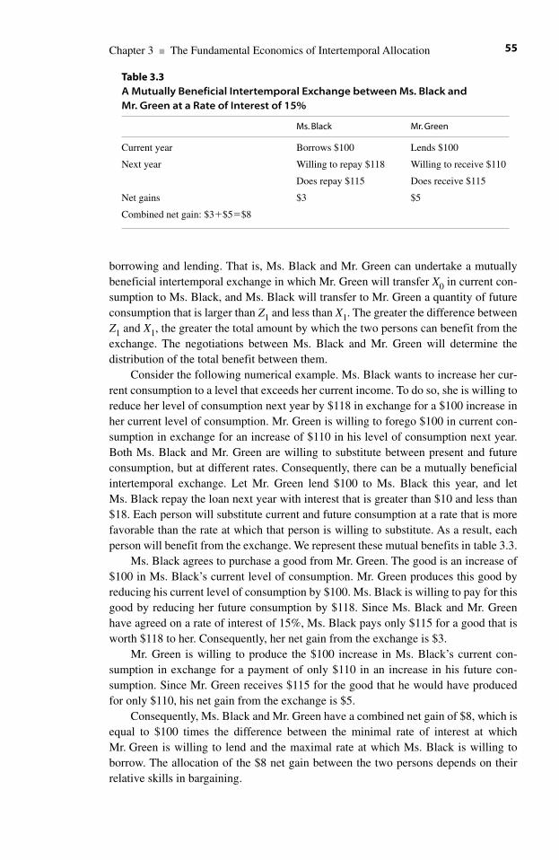
borrowing and lending. That is, Ms. Black and Mr. Green can undertake a mutuallybeneficial intertemporal exchange in which Mr. Green will transfer X0 in current con-sumption to Ms. Black, and Ms. Black will transfer to Mr. Green a quantity of futureconsumption that is larger than Z1 and less than X1. The greater the difference betweenZ1 and X1, the greater the total amount by which the two persons can benefit from theexchange. The negotiations between Ms. Black and Mr. Green will determine thedistribution of the total benefit between them.

Consider the following numerical example. Ms. Black wants to increase her cur-rent consumption to a level that exceeds her current income. To do so, she is willing toreduce her level of consumption next year by $118 in exchange for a $100 increase inher current level of consumption. Mr. Green is willing to forego $100 in current con-sumption in exchange for an increase of $110 in his level of consumption next year.Both Ms. Black and Mr. Green are willing to substitute between present and futureconsumption, but at different rates. Consequently, there can be a mutually beneficialintertemporal exchange. Let Mr. Green lend $100 to Ms. Black this year, and let Ms. Black repay the loan next year with interest that is greater than $10 and less than$18. Each person will substitute current and future consumption at a rate that is morefavorable than the rate at which that person is willing to substitute. As a result, eachperson will benefit from the exchange. We represent these mutual benefits in table 3.3.

Ms. Black agrees to purchase a good from Mr. Green. The good is an increase of$100 in Ms. Black’s current level of consumption. Mr. Green produces this good byreducing his current level of consumption by $100. Ms. Black is willing to pay for thisgood by reducing her future consumption by $118. Since Ms. Black and Mr. Greenhave agreed on a rate of interest of 15%, Ms. Black pays only $115 for a good that isworth $118 to her. Consequently, her net gain from the exchange is $3.

Mr. Green is willing to produce the $100 increase in Ms. Black’s current con-sumption in exchange for a payment of only $110 in an increase in his future con-sumption. Since Mr. Green receives $115 for the good that he would have producedfor only $110, his net gain from the exchange is $5.

Consequently, Ms. Black and Mr. Green have a combined net gain of $8, which isequal to $100 times the difference between the minimal rate of interest at whichMr. Green is willing to lend and the maximal rate at which Ms. Black is willing toborrow. The allocation of the $8 net gain between the two persons depends on theirrelative skills in bargaining.


Table 3.3A Mutually Beneficial Intertemporal Exchange between Ms. Black and Mr. Green at a Rate of Interest of 15%

Ms. Black Mr. Green

Current year Borrows $100 Lends $100

Next year Willing to repay $118 Willing to receive $110

Does repay $115 Does receive $115

Net gains $3 $5

Combined net gain: $3�$5�$8

Since both Ms. Black and Mr. Green gain by lending and borrowing $100 at 15%,we would expect both persons to expand the amount that they lend and borrow. AsMs. Black increases her current consumption at the expense of reducing her futureconsumption, we would expect her to reduce the maximal rate of interest that she iswilling to pay. Similarly, as Mr. Green increases his future consumption at the expenseof reducing his current consumption, we would expect him to increase the minimalrate of interest that he is willing to accept.3 Equilibrium occurs when the two ratescoincide. At that point, neither person has an incentive to undertake any furtherexchanges between present and future consumption.

If Ms. Black and Mr. Green are the only persons in the economy, they can proba-bly locate and negotiate with each other directly. But in an economy that has a largepopulation of persons who differ in their willingness to substitute between present andfuture consumption, financial markets can substantially decrease the costs of effectingintertemporal exchanges. Any reduction in the costs of producing a good will increasethe quantity of that good produced and consumed. Mutually beneficial intertemporalexchanges are no exception. Consequently, the existence and operation of financialmarkets increase the welfare of those members of the society who participate, directlyor indirectly, in mutually beneficial intertemporal exchanges.4

Consider, for example, the market for mortgaged loans used to finance the construc-tion of new homes and the purchase of existing homes. The borrowers in this market payinterest to the lenders over many years. The interest is the price that a borrower pays forearly access to a home,5 rather than postponing access until he or she can accumulateenough savings to purchase a home without a loan. Thus, by paying interest a borrowersubstitutes an increase in present consumption for a decrease in future consumption.The lenders substitute in the opposite direction. By advancing the loan, the lenders reducetheir current consumption. As the loan is repaid with interest, the lenders can increasetheir future consumption relative to what it would have been had they not made the loan.

The mortgaged loans effect mutually beneficial exchanges between the borrowersand the lenders. The lenders are the bank’s depositors. Banks facilitate these exchangesby reducing the costs that the borrowers and the lenders would otherwise incur. One ofthe costs for a lender is the risk that the borrower might not repay the loan (or notrepay on time). Banks reduce this cost for lenders partly by investigating the credit-worthiness of prospective borrowers and partly by enabling the lenders (the bank’sdepositors) to diversify their lending across several borrowers. Similarly, the costincurred by a borrower to arrange a loan with a bank is lower than the cost he or shewould incur if he or she negotiated with a set of lenders directly.

Without banks, many potential mutually beneficial exchanges would not beattempted because the costs of effecting these exchanges would exceed the benefits.The market for mortgaged loans is just one example.

We know that two persons can benefit from an intertemporal exchange only ifthey are willing to substitute between present and future consumption at differentrates. We know also that the larger the difference in the rates at which two persons arewilling to substitute between present and future consumption, the greater is the bene-fit that they can share.

We assume that every person is willing to forego some current consumption inexchange for a sufficiently large increase in future consumption. That is to say, every


person would agree to lend if the rate of interest were sufficiently high. Similarly,every person is willing to increase current consumption in exchange for a sufficientlysmall decrease in future consumption. This means that every person would borrow ifthe rate of interest were sufficiently low. It is likely that the larger the number of per-sons in an economy, the larger will be the variation among those persons in the rates atwhich they are willing to substitute intertemporally. Therefore, the larger the numberof persons in the economy, the greater the incentive for any one person to search foranother person whose willingness to substitute differs substantially from his or herown. Financial markets reduce the costs of these searches, and thereby increase theextent to which the potential benefits from mutually beneficial intertemporalexchanges are realized.

3.3.3 The Rise of Markets

We have seen that individuals can increase their levels of lifetime utility by makingintertemporal allocations of their scarce resources, and by entering agreements withother individuals for specialization and exchange according to the theory of compara-tive advantage. Individuals could do these two things without creating firms.

For most goods and services, however, the development of technology since theIndustrial Revolution has enabled owners of resources to obtain the benefits of spe-cialization and exchange more efficiently by pooling their resources in firms than byoperating those resources separately. Part of the reason is that the opportunities forspecialization have become more numerous and more sophisticated. Also, much of thenew technology favors the use of production on a large scale. Over time, technologyhas become both more complex and more dependent on large commitments of capitalfor long periods of time. For these reasons, technological development has increasedthe demand for financial markets because these markets reduce the costs of organizingintertemporal exchanges and accumulating capital goods. Without financial markets,many potential mutually beneficial intertemporal exchanges would be foregone.

3.4 The Assumption That Future Payments Are Known with Certainty Today

Introductory students know that economists often use simplified models to concen-trate on the essential aspects of a question. For example, to introduce the concept ofreal marginal opportunity costs, we assume that the economy produces only twogoods, X and Y, and that the economy’s production possibility frontier is smooth andconcave. Most economies, however, can produce more than two goods; it would beremarkable if all production possibility frontiers were smoothly concave. Even so, thesimple model of an economy that can produce only two goods provides a powerfulintroduction to critical analytical concepts. Indeed, this simplified model probablyenables introductory students to grasp more quickly the essential idea that the cost ofproducing an additional unit of Good X is the quantity of Good Y that must be fore-gone, and that the marginal cost of producing Good X increases as the economymoves rightward and downward along the frontier.


We know that financial economics is a study of how consumers maximize lifetimeutility by allocating resources among activities that will provide various levels ofpresent and future consumption. The future outcomes of these activities cannot, ingeneral, be known with certainty today. Individual consumers differ in their willing-ness to tolerate uncertainty. Therefore, consumers can increase their lifetime levels ofutility by entering into exchanges that shift risk from one person to another. Theseexchanges are claims to future levels of consumption that are conditional on futureoutcomes of various productive activities. The analysis of the pricing of these condi-tional claims is critical to understanding the economics of financial markets. Theanalysis is also complex. We can understand the analysis of these conditional claimsmore easily by first considering how a financial market will organize mutually benefi-cial exchanges under the simplifying assumption that there is no uncertainty aboutfuture outcomes. We can then exploit several analogies between the case in whichthere is no uncertainty about future outcomes and the more realistic case in whichthere is uncertainty.

3.5 Abstracting from Firms

By organizing their resources within firms, consumers can more fully exploit theopportunities for specialization and exchange provided by modern technology. Byissuing a variety of conditional claims on its future earnings, the modern corporationprovides a rich set of opportunities for mutually beneficial allocations of risk.Financial markets provide linkages between consumers and the firms that use the con-sumers’ resources to produce goods and services. Some of these linkages are informa-tional; consumers want to know what kinds of transformations their firms can makebetween the input of resources and the output of goods and services. Consumers alsowant to be able to enter mutually beneficial exchanges of risk with other consumerswho hold the firms’ securities. The markets provide these linkages by organizing thetrading, and thus the pricing, of a variety of financial securities.

The analysis of how, and how well, the financial markets provide these linkagesis the central task of this book. But it is a complex task. We can proceed best by firstabstracting from the fact that consumers use firms to organize the transformation ofinputs into outputs of goods and services. Doing so will enable us to concentrate onthe essential function of financial markets, which is to expand the range of mutuallybeneficial exchanges. By first abstracting from firms, we can more easily developthe analytical principles that we will use later when we do consider how financialmarkets link consumers and firms.

Of course, abstracting from firms will limit our analysis by excluding severalimportant problems. These problems include asymmetry of information betweena firm’s owners and managers, and conflicts of interest between owners and man-agers. We consider these problems later, after we have developed the fundamentalanalytical concepts that are essential to study these problems beyond a conversationallevel.


3.6 The Distinction between Income and Wealth

The first step in the analysis of the intertemporal maximization of utility is to distin-guish between income and wealth. Income is a flow of value, whereas wealth is astock of value. If Ms. Brown works for someone else in exchange for the payment ofmoney, her income is measured as a flow of dollars relative to some unit of time, suchas one year. If she is self-employed producing potatoes, her income is measured as aflow of potatoes produced per year. Ms. Brown will probably sell some or all of thepotatoes that she produces, thereby exchanging the form of her income from potatoesto money. But whatever the form in which she receives her income, that income is aflow, a measure of the value obtained (in some form) per year (or per some other unitof time).

Conversely, wealth is a stock of value. It is the result of an accumulation ofincome generated in the past or in the present. There are three forms in whichMs. Brown could hold wealth. The most primitive form of wealth is a stock of con-sumption goods. Ms. Brown could, for example, simply accumulate and store someof the potatoes that she produces each year. In any given year, the maximal quantityof potatoes that she could consume during that year (without borrowing fromanother consumer) would be equal to the total quantity of potatoes that she producesin that year, plus the volume of potatoes that she had accumulated during previousyears. That is to say, assuming again that she does not borrow, her consumptionwould be constrained by her current income and her accumulated wealth. In thisexample, her consumption, her income, and her wealth are all measured in terms ofpotatoes.

The second form in which Ms. Brown could hold wealth is money. For example,she can sell her entire output of potatoes in a given year, thereby converting herincome into money, and then save some of that income. That accumulation of incomewill increase her wealth. In future years, she can consume that wealth by spending themoney to purchase goods and services.

The third, and most sophisticated, form in which Ms. Brown could hold wealth isan accumulation of claims on income to be generated in the future. For example,Ms. Brown could give some of her current output of potatoes to Mr. Black, who wouldthen use them as seed potatoes to expand the scale on which he will produce potatoesnext year. In exchange for allowing Mr. Black to use some of her current output ofpotatoes as an input for future production, Ms. Brown will obtain from Mr. Black aclaim on a portion of his future output.

In a more sophisticated model of an economy, this claim would be saleable.Ms. Brown could sell the claim to someone else, rather than exercising it herself. Thissaleable claim would be a financial security. Financial markets would determine theprice of this security by reconciling the willingness of households to divert incomefrom current consumption and the ability of farmers like Mr. Black to use seed pota-toes to expand future levels of output. As a result, Ms. Brown and Mr. Black couldconstruct a mutually beneficial exchange.

In summation, the ideas to keep in mind are that income is a flow, and that wealthis a stock acquired by accumulating income that is not spent for consumption.


3.7 Income, Wealth, and Present Values

In the next section, we analyze a simple case in which a consumer uses a financialmarket to borrow or lend, and thereby to allocate resources between present and futureconsumption so as to maximize lifetime utility. To prepare for this analysis, we mustfirst develop the concept of present value.

3.7.1 Present Value

A present value is a stock of wealth that is economically equivalent to a future flow ofincome. Precisely, the present value of a particular flow of income is that level ofwealth that would enable a person to replicate that flow of income.

Consider the following examples. Mr. Green’s income is $110 per year for twoyears. He will receive his first payment of $110 today, and he will receive his secondand final payment of $110 one year from today. The present value of Mr. Green’ssequence of income payments is the level of wealth that Mr. Green must have today ifhe is to replicate the sequence of income payments. If we ignore the possibility thatMr. Green can invest any wealth today and receive interest next year, the answer issimple. Mr. Green would have to possess $220 in wealth today in order to replicatetwo payments of $110 each.

But suppose that Mr. Green can earn interest at the rate of 10% per year by plac-ing money on deposit in a bank. In this case, a deposit of $100 in a bank today willgrow to $110 one year from today. Therefore, Mr. Green could provide for the pay-ment of $110 next year by depositing only $100 in a bank today. Economists wouldsay that Mr. Green could fund an opportunity to receive $110 one year from today bydepositing $100 in a bank account today.

Our question: how much money must Mr. Green have today to enable him toreplicate the flow of income that provides $110 today and a second $110 one yearfrom today? The answer depends on the rate at which Mr. Green can earn interest bydepositing money in a bank. If the interest rate is 10% per year, then Mr. Green willrequire $210 today if he is to replicate the payments of $110 today and a second $110one year from today. Mr. Green would use $110 of the $210 to make the first payment.He would then deposit the remaining $100 ($210 � $110) in a bank today. One yearfrom now, he could withdraw a total of $110, counting both the original deposit andthe interest at the rate of 10% on that deposit. He could then use that $110 to make thesecond payment.

We conclude that if Mr. Green can earn interest at the rate of 10% per year, then$210 is the present value of the flow of income that pays $110 immediately and a sec-ond $110 one year from today. It is easy to see that the present value of a flow ofincome varies inversely with the interest rate. Suppose that the interest rate were 5%per year. Clearly Mr. Green would have to deposit more than $100 today if the accountis to grow to $110 by next year. Let D0 be the amount that must be deposited today tofund a payment equal to P1 one year from today. Let r be the annual rate of interestpaid by the bank. Then D0, P1, and r are related by

D0(1�r)�P1 (3.1)


or

D0�P1/(1+r). (3.2)

For our example, if the bank pays interest at 5% per year, Mr. Green would haveto deposit $110/(1�.05), or $104.76 today if he is to use this bank account to fund apayment of $110 one year from today.

We will now consider the concept of present value for two more general cases. Inthe first case, the flow of income consists of a sequence of payments that continues fora finite number of years into the future. In the second case, the sequence of paymentscontinues forever.

3.7.2 A Sequence with Two Future Payments

Define Pi as the payment that will occur i years from now. The values of the indexi are restricted to nonnegative integers. Thus, P0 is the payment that will occur todayand P1 is the payment that will occur one year from today, and so on.

Let r be the annual rate of interest paid by a bank, and assume that this interest iscompounded annually. Then a deposit today equal to D0 will grow to D0(1�r)1 at theend of one year. Define this value as D1. That is, D1�D0(1�r)1. If an amount ofmoney equal to D1 is deposited in a bank one year from now and allowed to accumu-late interest at rate r for one year, then the account will grow to D1(1�r)1 at the end oftwo years from now. Define D2�D1(1�r)1. Then by substitution we have:

D2�D1(1�r)1�D0(1�r)1(1�r)1�D0(1�r)2. (3.3)

That is, if D0 is deposited in a bank today and allowed to accumulate interest for two years at a compound annual rate equal to r, the value of the account at the end oftwo years will be D0(1�r)2. Of course, for the initial deposit of D0 to grow to a valueof D0(1�r)2 at time 2, the entire initial amount of D0 must be left on deposit for the entire two years; there must be no withdrawal of any part of the initial deposit attime 1.

In general, if D0 is deposited in a bank today and allowed to accumulate interestfor i years at a fixed compound annual rate equal to r, and there are no withdrawals,the value of the account at the end of i years will be D0(1�r)i.

We can now invert the preceding relationships to calculate the present value of afuture payment.

By definition, the present value of a flow of payments is the amount of currentwealth that would enable a person to replicate the flow of payments. Suppose that theflow of payments consists of a single payment, namely, a payment equal to P1 oneyear from now. Using our earlier calculations, we know that the present value of P1 isP1/(1�r]1. That is, a deposit equal to P1/(1�r)1 today will grow to a value equal to[P1/(1�r)](1�r)�P1 one year from today. Therefore, the amount of wealth that a per-son would need today to replicate a payment equal to P1 one year from today isP1/(1�r)1. We say that P1/(1�r)1 is the present value of P1. Note that the person whois replicating this payment would withdraw from the bank one year from today boththe initial deposit and the accumulated interest. There is no need to leave any moneyon deposit in the bank because there are no further payments to replicate after time 1.


Next consider a second sequence that has only one payment. This payment occurstwo years from now. Call this payment P2. We want to determine the size of thedeposit that a person would have to make today in order to be able to withdraw anamount equal to P2 two years from now. This deposit today, plus the interest accumu-lated over two years, would replicate the payment of P2. Consequently, an investorshould be indifferent between owning today a sequence that will pay P2 two yearsfrom now, and owning today a bank account that will enable him or her to replicatethat payment.

Let X be the amount of the bank deposit today that would enable a person toreplicate the payment of P2 two years hence. We know that a deposit equal to Xtoday will grow in value to X(1�r)2 two years from today if there are no with-drawals before that time. Setting the value to which the account will grow equal tothe future payment that we want to replicate, we have X(1�r)2�P2. Therefore,X�P2/(1�r)2. That is, a deposit equal to P2/(1�r)2 today will grow to a value equalto [P2/(1�r)2](1�r)2�P2 at time 2. The person who makes the initial deposit ofP2/(1�r)2 would make no withdrawal at time 1. At time 2, the person would with-draw the entire balance in the account. There is no need to withdraw any funds attime 1 because there is no payment to replicate then, and there is no need to leave anymoney on deposit after time 2 because there are no further payments to replicate aftertime 2.

Since a deposit of X today will enable the depositor to replicate the payment of P2two years from today, X�P2/(1�r)2 is the present value of P2.

Now consider a third sequence. In this sequence there are two future payments,namely, a payment equal to P1 at time 1, and a payment equal to P2 at time 2. There areno further payments. It is easy to show that the present value of this sequence of pay-ments is the sum of the present values of each of the two future payments consideredseparately. First, note that a person could replicate these two payments simply bymaking two deposits today in separate accounts. A deposit of P1/(1�r)1 in oneaccount will grow to a value equal to P1 at time 1. A deposit of P2/(1�r)2 in a secondaccount will grow to a value equal to P2 at time 2. The person who is replicating thetwo payments simply withdraws the entire balance from each account, including theaccumulated interest, at the designated time.

We can accomplish the same result by depositing the sum of the two presentvalues in a single account. At time 1 we will withdraw an amount equal to P1 fromthe account. The amount remaining in the account will then grow in value to theamount of the second payment, P2, at time 2. Following is a demonstration of thisresult.

Define B0 as the balance in the account at time 0. Define Bi as the balance in theaccount at time i after taking into account (1) whatever withdrawals were made priorto time i, and (2) whatever interest has been allowed to accumulate. The withdrawalswill be the two payments that we want to replicate, namely, P1 at time 1, and P2 attime 2. The balance at time 0, B0, is the sum of the present values of the two payments.Thus,

(3.4)BP

r

P

r0

11

22(1 ) (1 )

.��

��


At time 1 the balance will have grown to:

(3.5)

After withdrawing the amount P1 at time 1 to make the first payment in thesequence, the balance in the account will be equal to P2/(1�r)1. This balance willaccumulate interest from time 1 to time 2. Therefore, the balance at time 2, before anywithdrawals at time 2, will be

(3.6)

The balance remaining in the account at time 2 will be P2, which is exactly what isrequired to replicate the final payment in the sequence. Withdrawing this amount willexhaust the account, which is appropriate because there are no further payments toreplicate after time 2.

3.7.3 A Numerical Example

Consider the following example. Ms. Black finds a new job in which she will be guaran-teed a series of income payments. Although she will receive no payment today, she willreceive a payment of $150 one year from today, and a second payment of $180 two yearsfrom today. Following the second payment, Ms. Black will receive no further income.

What amount of money must Ms. Black possess today in order to replicate thissequence of payments? In the absence of investment opportunities, the answer is clear:she must have $330. However, suppose Ms. Black is presented with the followingoption: by depositing her money in a nearby bank, she can earn interest on her depositat a rate of 5% per year. How much money must she have to replicate the sequence ofpayments provided by the job?

One method by which she could replicate this flow of income is to make twodeposits today in separate accounts. As we learned in section 3.7.2, if Ms. Black depositsthe present value of her first payment [P1/(1�.05)1 or $142.86], her balance will grow to$150 at time 1. Similarly, by depositing $163.27 [the present value P2/ (1�.05)2 of hersecond payment], Ms. Black’s balance will grow to $180 at time 2. Ms. Black need onlywithdraw the entire balance from each account at the appropriate time.

However, Ms. Black need not hold two separate accounts. Instead, she may opena single account with a balance that equals the sum of the present values of her twopayments. Using equation (3.4), we know that balance at time 0 must be $306.13.With an interest rate of 5%, at time 1 the balance will have grown to $321.44.

At time 1, Ms. Black will withdraw the amount necessary to make the first pay-ment, namely $150. Consequently, the remaining balance will be $171.44. This balancewill continue to gain interest from time 1 to time 2. Before Ms. Black makes her secondwithdrawal, her account will contain $180, the exact amount of her second payment.

BP

rr P2

21

12

(1 )(1 ) .�

��

BP

r

Pr

PP

r

11

12

21

12

1

(1 ) (1 )(1 )

(1 ).

��

��

�

� ��

r

⎡

⎣⎢

⎤

⎦⎥


As there are no further payments necessary to replicate the sequence, Ms. Black hasemptied her account.

We return to the original question. With the option to invest her money at anannual interest rate of 5%, how much money must Ms. Black have today if she is toreplicate the sequence of payments? The answer is the sum of the present values ofboth payments: $306.13.

3.7.4 A Sequence with an Infinite Number of Uniform Payments

We finally consider a sequence in which the payments are uniform and continue forever.The sequence provides a constant payment at the rate of P per year, beginning one yearfrom today and continuing forever. The present value of this sequence is the amount ofcurrent wealth that would enable a person to replicate the sequence. Since the sequenceof payments continues forever, we can replicate it by maintaining a balance in a bankaccount on which the annual interest is equal to the annual payment that we want toreplicate. If the rate of interest is constant over time, then the required balance in theaccount will be constant (after allowing for the annual withdrawal of interest).

Again, define B0 as the amount of money to be deposited at time 0. If the annualrate of interest is r, the value of the account at time 1, prior to any withdrawals, will beB1�B0(1�r)1�B0�rB0. Obviously, the balance at time 1 consists of the initialdeposit B0 plus the interest for one year on that deposit, rB0. If we withdraw only theinterest at time 1, we will leave a balance equal to B0 on which to earn interest fromtime 1 to time 2. The interest at time 2 will be the same as it was at time 1, namely rB0,because the balance on which we can earn interest over the second year is the same asthe balance on which we earned interest over the first year. In general, by depositingB0 at time 0 and withdrawing only the interest each year, we can replicate an infinitesequence of payments equal to rB0 per year. Therefore, the amount of current wealthB0 that would enable us to replicate an infinite sequence of annual payments equal toP when a bank pays interest at a rate of r per year is determined by the equationrB0�P. The solution is B0�P/r.

A numerical example will make this transparent. If the bank pays interest at therate of 10% per year and the annual payment in the sequence is equal to $100, then adeposit equal to $100/.10�$1,000 will enable us to replicate the sequence. Leavingthe $1,000 in the bank permanently will enable us to withdraw $100 per year forever,which is identical to the sequence that we want to replicate.

3.7.5 Present Values and Economic Equivalence

The present value of a sequence of future payments is also known as the capitalizedvalue of that sequence. The reason is that the present value is the amount of financialcapital required to replicate that sequence of payments. We know that the presentvalue is the amount of current wealth that would enable a person to replicate thesequence. Wealth is a stock (rather than a flow). One of the forms in which a personcan hold wealth is a bank account. The balance in the account is part of the person’sfinancial capital. Hence, the capitalized value of a sequence of future payments is thestock of financial capital that would enable a person to replicate the sequence.


The present value of a sequence is a stock; it is the quantity of wealth that a per-son must have now if he or she is to replicate that sequence. The sequence itself is aflow; it is measured as payments per year (or per some unit of time) over some inter-val of years into the future. The future payments need not be equal from one year tothe next, nor need they continue indefinitely into the future. As we saw earlier, thesequence could contain only one future payment.

We now introduce the concept of economic equivalence between sequences ofpayments. Two sequences are economically equivalent if they have the same presentvalue. If two sequences are economically equivalent, an investor who owns eithersequence, and who can borrow from and lend to a bank, can use the payments in thatsequence to replicate the payments in the other sequence without committing any ofhis own funds. Therefore, an investor will be indifferent between owning sequencesthat are economically equivalent. As a particular application of this concept, note thatusing one’s own money to purchase a sequence produces the same result as purchas-ing that sequence by using money borrowed from a bank.

The capitalized value (or present value) of a sequence of payments, and thesequence of payments itself, are economically equivalent in the sense that anyone whoowns the right to receive the payments in the sequence can exchange that right for itscapitalized value. The converse also holds. This concept of economic equivalence will beimportant throughout the book. For that reason, we pause here to provide two examples.

Let the annual interest rate be 10%, and consider the sequence of three paymentsspecified by P1 � $110, P2 � $121, and P3 � $133.10. The capitalized value of thissequence is:

(3.7)

A person who owns the right to the sequence that will pay $110 at time 1, $121 attime 2, and $133.10 at time 3 could sell the right to that sequence for $300. To showthis, suppose that the person offered to sell the sequence for $290. A second personcould borrow $290 from a bank and use that money to purchase the sequence. At time 1, the borrower would owe the bank the $290 plus interest for one year, or$290(1�.10)1 � $319. But the borrower could use the first payment from the sequenceto reduce his indebtedness to the bank. Doing this would reduce his debt to$319 � $110, or $209.

If the borrower used the second payment from the sequence to pay down the debt, he or she would owe the bank at time 2 the amount $209(1 �.10)1 � $121�

$229.90 � $121 � $108.90.At time 3, the debt will be $108.90(1�.10)1 � $119.79, which is less than what

the borrower will receive as the third (and final) payment in the sequence. Therefore,

BP

r

P

r

P

r0

11

22

33

1 2

(1 ) (1 ) (1 )

$110

(1 .10)

$121

(1 .10)

$1

��

��

��

��

��

�333.10

(1 .10)

$110

1.1

$121

1.21

$133.10

1.331$100 $100 $10

3�

� � �

� � � 00

$300.�


the borrower will obtain a net profit at time 3 equal to $133.10�$119.79�$13.31.This profit arises because, at $290, the sequence that pays $110 at time 1, $121 at time2, and $133.10 at time 3 is underpriced, assuming that the interest rate is 10% per year.Competition among investors will drive the price of the sequence up to $300. Thereader should be able to show that an investor could not make a profit by borrowing$300 from a bank and purchasing the sequence. Obviously (and the reader should beable to show this), the sequence would be overpriced at any price above $300;investors who purchased the sequence for more than $300 would incur a loss.

But what if the investor uses his or her own funds to purchase the sequence, ratherthan borrowing from a bank? Students of economics will immediately recognize thatusing one’s own money to purchase the sequence, rather than depositing that money ina bank, incurs an opportunity cost in the form of interest foregone.

We have shown that an investor who owns a right to receive a sequence of payments can convert that right to its capitalized value. To show the converse, we rec-ognize that an investor can convert the capitalized value of a sequence into thesequence itself by depositing the capitalized value in a bank, and then by replicatingthe sequence with a series of withdrawals. Using the preceding example, let theinvestor deposit $300 today. That balance will grow to $300(1�.10)1�$330 at time 1. Withdrawing $110 at time 1 will leave $330�$110�$220 to accumulate interest between time 1 and time 2. At time 2, the balance in the account will be$220(1�.10)1�$242. Withdrawing $121 at time 2 will leave $121, which will growto $121(1�.10)1, or $133.10 at time 3. This last amount can be withdrawn at that timeto replicate the final payment in the sequence. This concludes our discussion of funda-mental analytical concepts involved in the intertemporal allocation of resources. Inchapter 4, we use these concepts in our presentation of the Fisher diagram of optimalintertemporal allocation.

Problems

1. LickIt Candy Company produces two types of candy: pops and gum. Thecompany has two plants, East Plant and West Plant. In West Plant, each machine canproduce 3 units of gum/hr or 2 units of pops/hr. In East Plant, each machine can pro-duce 5 units of gum/hr or 1 unit of pops/hr. What is the marginal cost of producing 15units of gum in East Plant? Which plant has a comparative advantage?

2. With Good X plotted horizontally, and Good Y plotted vertically, the slope ofMs. Tall’s production possibilities frontier is �2:1 while the slope of Ms. Short’sproduction possibilities frontier is �3:1. Who has a comparative advantage in termsof X and Y? Use a graph to explain your answer.

3. The First Bank is currently paying 10% interest compounded annually on alldeposits. Mr. Smith deposits $100 at t �0. How much would he need to deposit oneyear later at t �1 to have $275 in the bank the next year, at t �2? By how much wouldhe have to increase his deposit at t�0 in order to have $275 at t�2 without making adeposit at t �1?


4. Heart College charges students a different fee for each year of their education.The tuition for the first year is $2,200. Tuitions for the second, third, and fourth yearsare $2,420, $2,662, and $2,928.2, respectively. Each tuition payment is due at the endof the year for which it is paid. How much would Mr. Smith be willing to pay today tobuy the full four-year package if the interest rate is 10%?

Notes

1. We assume that the farmer allocates to current production, rather than to leisure, the timethat would have been spent on maintenance.

2. Most introductory courses in economics present the theory of comparative advantage. Forthat reason, we present only a simple example here.

3. These changes in the maximal and minimal rates of interest are an example of the axiomknown as “diminishing marginal rate of substitution.” Under this axiom, the marginal rate atwhich a person is willing to substitute less of Good Y for an increase of one unit of Good Xdecreases as the total quantity of Good X that the person has increases.

4. A carpenter who neither borrows nor lends will still benefit from the operation of financialmarkets if, by using those markets, the construction firm that employs her can more easilyobtain loans with which to finance the construction of new homes.

5. The concept of interest as the price of early access to a good appears in A. Alchian andW. Allen, Exchange and Production: Theory in Use (Belmont, Calif.: Wadsworth, 1969), 265.



4.1 The Intertemporal Budget Line

We will develop a graphical tool to explain how a consumer determines the levels ofborrowing or lending to maximize lifetime utility.1 We begin with a simple model in which a person has only two periods in which to consume. The problem is to deter-mine the optimal allocation of resources between consumption this year and consumption next year. We will emphasize the informational function of financialmarkets that enables consumers to identify and create mutually beneficial intertempo-ral exchanges.

In figure 4.1, we measure levels of income and spending this year on the horizon-tal axis, and levels of income and spending next year on the vertical axis. Let time 0 bethe present moment; let time 1 be the moment that is exactly one year from now; andlet time 2 be the moment that is exactly two years from now. The current year beginsat time 0 and ends at time 1; the following year begins at time 1 and ends at time 2.The consumer will die at time 2.

The consumer’s flow of income consists of a sequence of payments, namely I0 attime 0, followed by I1 at time 1. We represent this sequence by {I0, I1}, which we plotin figure 4.1 as the point {I0, I1}.

Now define {C0, C1} as the sequence of the consumer’s spending. Unless theconsumer is a miser, whom we would define as a person whose ultimate goal is toacquire money rather than goods and services, the consumer obtains utility only byusing her income to acquire consumption goods. The consumer now has two prob-lems. The first problem is intertemporal; she must allocate her spending optimallybetween the current year and the following year. The second problem is to allocate herspending for each year optimally among the various goods and services that are avail-able to purchase within that year. We will abstract from this second problem, andanalyze only the first problem.

The consumer’s problem of intertemporal allocation arises because the sequenceof expenditures for consumption, {C0, C1}, that will maximize her lifetime utility willnot, in general, correspond to the sequence of her income flows, {I0, I1}. For example,if the consumer is a recent college graduate, her current income, I0, is likely to be quitelow relative to her future income, I1. It is likely that she would prefer to reallocate someof her future income to the present so that she can have a better distribution of her life-time income between consumption this year and consumption next year. In particular,she might prefer to use some of her future income to purchase a house now, and then

4 The Fisher Diagram for OptimalIntertemporal Allocation

69

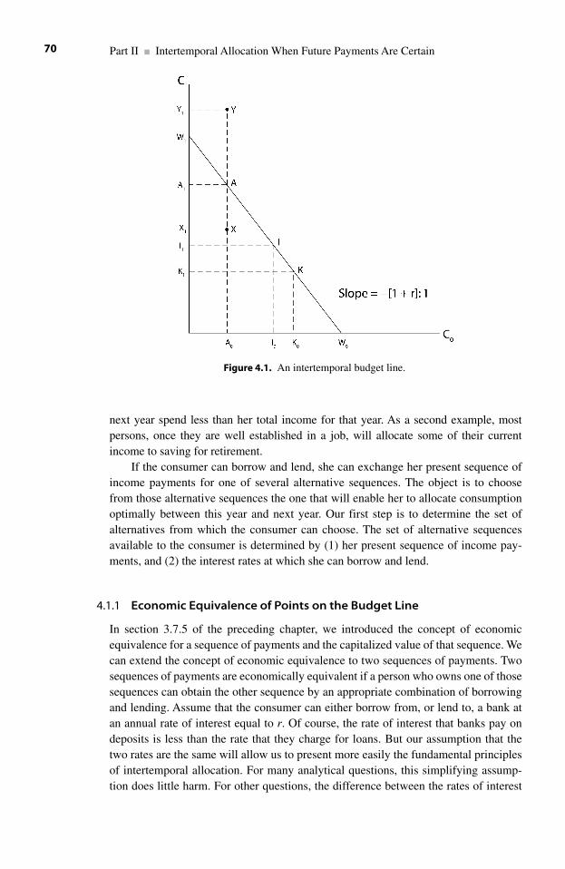
next year spend less than her total income for that year. As a second example, mostpersons, once they are well established in a job, will allocate some of their currentincome to saving for retirement.

If the consumer can borrow and lend, she can exchange her present sequence ofincome payments for one of several alternative sequences. The object is to choosefrom those alternative sequences the one that will enable her to allocate consumptionoptimally between this year and next year. Our first step is to determine the set ofalternatives from which the consumer can choose. The set of alternative sequencesavailable to the consumer is determined by (1) her present sequence of income pay-ments, and (2) the interest rates at which she can borrow and lend.

4.1.1 Economic Equivalence of Points on the Budget Line

In section 3.7.5 of the preceding chapter, we introduced the concept of economicequivalence for a sequence of payments and the capitalized value of that sequence. Wecan extend the concept of economic equivalence to two sequences of payments. Twosequences of payments are economically equivalent if a person who owns one of thosesequences can obtain the other sequence by an appropriate combination of borrowingand lending. Assume that the consumer can either borrow from, or lend to, a bank atan annual rate of interest equal to r. Of course, the rate of interest that banks pay ondeposits is less than the rate that they charge for loans. But our assumption that thetwo rates are the same will allow us to present more easily the fundamental principlesof intertemporal allocation. For many analytical questions, this simplifying assump-tion does little harm. For other questions, the difference between the rates of interest


Figure 4.1. An intertemporal budget line.

that banks will pay on deposits or charge for loans is critical. To analyze those ques-tions, economists use different models.

The straight line in figure 4.1 that passes through the point I is the set of alterna-tive sequences of income payments that are economically equivalent to the sequence{I0, I1}. If the consumer can borrow or lend at an annual rate of interest equal to r, shecan exchange any sequence of income payments that lies on this line for any othersequence that lies on the same line. This straight line is called the consumer’sintertemporal budget line. The slope of this budget line is �(1�r): 1.

There is a close analogy between a production possibility frontier for the economyand an intertemporal budget line for a consumer. Both a production possibility frontierand an intertemporal budget line define trade-offs that are conditional on levels ofscarce resources. A production possibility frontier defines the alternative combinationsof goods that an economy can produce in a single year, given the level of resources onwhich the economy can draw. These resources include tangible inputs, such as land andrailroad equipment, and intangible inputs, such as technological knowledge and thelevel of technological sophistication in the labor force. An intertemporal budget linedefines the alternative combinations of current and future consumption that a personcan enjoy, given his or her current level of wealth and the interest rate. The level ofresources available to the economy in a given year is analogous to the individual’s levelof wealth at the beginning of a year. The state of the technology is analogous to theinterest rate. Technology specifies the rates at which the economy can substitutebetween goods by producing more of one and less of another. The interest rate specifiesthe rate at which an individual can substitute between current and future consumptioneither by borrowing or by lending.

Consider the sequence {A0, A1} that lies at point A on the budget line. By lending,the consumer can trade her present sequence of income payments, {I0, I1}, for thesequence {A0, A1}. It is easy to see why this is true. The slope of the budget line is�(1�r). Therefore, using the definition of slope as “rise over run”:

(4.1)

so that

(4.2)

and

(4.3)

In equation (4.3), the term (I0�A0) is the amount by which the consumer reducesher level of current consumption below her current income. If the rate of interest is r,the future value of (I0�A0) is (1�r)(I0�A0). Consequently, equation (4.3) states thatthe consumer’s level of consumption next year, A1, is equal to her future income I1plus (1�r)(I0�A0), which is the future value of the decrease in her current level ofconsumption. At time 1, the consumer supplements her income by withdrawing fromthe bank both her deposit of (I0�A0) and the accumulated interest of r (I0�A0). Thatis, the consumer can lend to a bank to move upward and leftward along her intertem-poral budget line. In doing so, she is reallocating her resources from current consump-tion to future consumption.

A I r I A1 1 0 0(1 )( ).� � � �

A I r A I1 1 0 0(1 )( ),� ��

A I

A Ir1 1

0 0

(1 ),�

�� 2

Chapter 4 ■ The Fisher Diagram for Optimal Intertemporal Allocation 71

Rewriting equation (4.3) produces

(4.4)

which states that the amount by which the consumer must decrease her current con-sumption is (A1�I1)/(1�r), or the present value of the amount by which she willincrease her future consumption beyond her future income.

We have just seen how the consumer can use lending to a bank to move leftwardand upward along her intertemporal budget line. Alternatively, the consumer can useborrowing (from a bank) to reallocate resources from future consumption to currentconsumption. That is, she can move rightward and downward along her budget line.Consider the sequence at point K. At point K the consumer spends on consumption thequantities K0 this year and K1 next year. Proceeding as before, we have:

(4.5)

so that

(4.6)

and

(4.7)

In equation (4.7), the term (K0�I0) is the amount that the consumer borrowstoday in order to increase her current consumption above her current income.Consequently, the term (I1�K1) is the amount by which she must decrease her con-sumption next year in order to pay off her loan. If the interest rate is r, then (I1�K1)must be the future value of (K0�I0). That is, (I1�K1)�(1�r)(K0�I0). Students shouldnote that it is also possible for the consumer to operate at point X, where she consumesX0 in the current year and X1 in the following year. This combination of consumption,however, is not favorable. The consumer is not using all of her resources, and thus not maximizing utility. Should she decide to only consume A0 in the present year, her budget will allow her to consume more than X1 in the next year, namely A1.Conversely, it is not possible for her to function at a point such as Y. Even throughborrowing and lending, she does not have enough resources to have the combinationof present and future consumption represented by point Y.

4.1.2 Interpreting the Intercepts and the Slope of the Budget Line

To continue our graphical analysis of a consumer’s intertemporal allocation betweenpresent and future consumption, we need an economic interpretation of the interceptsof the intertemporal budget line.

Let W0 be the horizontal intercept of the intertemporal budget line in figure 4.1.Accordingly, W0 is the maximal level of current consumption that the consumer can

I K

rK I1 1

0 0(1 ).

�

��

K I

rK I1 1

0 0(1 )

�

� �� ,

K I

K Ir1 1

0 0

(1 ),�

��

I AA I

r0 01 1

(1 )� �

�

�,


afford if she spends all of her current income, I0, plus I1/(1�r), which is the presentvalue of her future income. Proceeding as before, we have:

(4.8)

so that

(4.9)

and thus

(4.10)

Let W1 be the vertical intercept of the consumer’s intertemporal budget line. ThenW1 is the maximal amount of future consumption that the consumer can afford if she spends none of her current income. If she deposits her entire current income of I0in a bank today, the value of her account at time 1 will be I0(1�r). At time 1, the max-imal amount that she can spend is the sum of this bank balance, plus the income I1 thatshe will have at time 1. Then W1�I1�I0(1�r). That is, her maximal level of consump-tion at time 1 is the sum of her income at time 1 plus the future value of her income attime 0.

We know that a sequence of payments and its present value are economicallyequivalent. This means that by either borrowing or lending, a person who has anamount of current wealth equal to the present value of the sequence can replicate thatsequence, and conversely, a person who owns the right to receive the payments in thesequence can exchange that sequence for its present value. We can use this fact tointerpret the intertemporal budget line in figure 4.1.

The horizontal intercept of the budget line represents a sequence of expendituresfor consumption equal to {W0, 0}. That is, the consumer spends in the current year herentire current income, I0, and the present value of her future income, I1. The presentvalue of I1 is I1/(1�r)1. A consumer who borrows I1/(1�r)1 from a bank today willowe the bank [I1/(1�r)1](1�r)1, which is equal to I1. Since the consumer will requireher entire income next year to repay the bank, her level of consumption next year willbe zero.

The economic interpretation of the vertical intercept of the budget line in figure4.1 is analogous to the interpretation of the horizontal intercept. The vertical interceptis the maximal level of consumption that the consumer can achieve next year if sheconsumes nothing this year. Let W1 be the value of the vertical intercept. Then thesequence of consumption expenditures that is represented by the vertical intercept is{0, W1}. To achieve the consumption sequence {0, W1}, the consumer must consumenothing this year and allocate her entire current income to investment. Specifically,the consumer deposits her current income, I0, in a bank at time 0. Next year, at time 1,her balance at the bank will have grown to I0(1�r)1. Adding this balance to herincome at time 1 will enable her to consume at time 1 at the level of I0(1�r)1�I1.Therefore, W1, which is the future value (at time 1) of the income sequence {I0, I1}, isequal to I0(1�r)1�I1.

�

� ��

��

I

rI

I

rI W1

01

0 0(1 ) (1 ).

� �� I r W I1 0 0(1 )( ),

0(1 ),1

0 0

�

��

I

W Ir


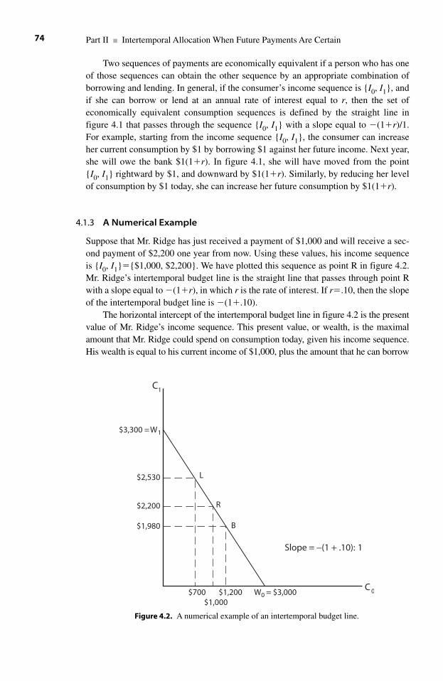
Two sequences of payments are economically equivalent if a person who has oneof those sequences can obtain the other sequence by an appropriate combination ofborrowing and lending. In general, if the consumer’s income sequence is {I0, I1}, andif she can borrow or lend at an annual rate of interest equal to r, then the set of economically equivalent consumption sequences is defined by the straight line in figure 4.1 that passes through the sequence {I0, I1} with a slope equal to �(1�r)/1.For example, starting from the income sequence {I0, I1}, the consumer can increaseher current consumption by $1 by borrowing $1 against her future income. Next year,she will owe the bank $1(1�r). In figure 4.1, she will have moved from the point {I0, I1} rightward by $1, and downward by $1(1�r). Similarly, by reducing her levelof consumption by $1 today, she can increase her future consumption by $1(1�r).


Suppose that Mr. Ridge has just received a payment of $1,000 and will receive a sec-ond payment of $2,200 one year from now. Using these values, his income sequenceis {I0, I1}�{$1,000, $2,200}. We have plotted this sequence as point R in figure 4.2.Mr. Ridge’s intertemporal budget line is the straight line that passes through point Rwith a slope equal to �(1�r), in which r is the rate of interest. If r�.10, then the slopeof the intertemporal budget line is �(1�.10).

The horizontal intercept of the intertemporal budget line in figure 4.2 is the presentvalue of Mr. Ridge’s income sequence. This present value, or wealth, is the maximalamount that Mr. Ridge could spend on consumption today, given his income sequence.His wealth is equal to his current income of $1,000, plus the amount that he can borrow


$700$1,000

$1,200 W0 = $3,000

$2,530

$2,200

$1,980

$3,300 = W1

C 0

C1

Slope = −(1 + .10): 1

L

B

R

Figure 4.2. A numerical example of an intertemporal budget line.

today against the income that he will receive next year. The present value of this futureincome is $2,200/(1�.10), or $2,000. We conclude that Mr. Ridge’s wealth is equal to$1,000�$2,200/(1�.10) � $3,000. He can spend $3,000 today by augmenting hiscurrent $1,000 by borrowing $2,000 from a bank; next year he will owe the bank$2,200. Paying the bank will absorb his entire future income. Consequently, the cost thatMr. Ridge would incur to increase his current consumption by $2,000 beyond his cur-rent income is that he must reduce his future consumption to zero.

The vertical intercept of Mr. Ridge’s intertemporal budget line is the future value of his income sequence. This future value is the maximal level at which he canconsume next year if he reduces his current consumption to zero. By depositing hisentire current income of $1,000 in a bank today, next year Mr. Ridge will have$1,000(1�.10), or $1,100, with which to augment his future income of $2,200. Weconclude that the maximal level of future consumption that his income sequence willsupport is $1,000(1�.10)�$2,200, or $3,300, which is the value of the vertical inter-cept of the intertemporal budget line in figure 4.2.

Points B and L on the budget line in figure 4.2 designate two of the infinite num-ber of alternative combinations of current and future consumption that Mr. Ridge canachieve when his income sequence is {$1,000, $2,200} and the interest rate is .10.Point B requires that he borrow, whereas point L requires that he lend. If Mr. Ridgeneither borrows nor lends, he must accept the combination of present and future con-sumption that is identical to his income sequence. To choose the combination at pointB, he would borrow $200 from a bank today. Next year he would have to use $220 ofthe $2,200 that he would receive to repay the bank. Consequently, his future consump-tion at point B would be $2,200�$220�$1,980. Notice that the rate at which Mr. Ridgemust forego future consumption per dollar of increase in current consumption is(�)$220/$200, or �1.1, which we can write as �(1�.10)/1. The interest rate speci-fies the rate at which Mr. Ridge can substitute between future and current consump-tion by determining the slope of his intertemporal budget line.

Alternatively, to move from point R to point L, Mr. Ridge would lend. By spend-ing only $700 of his current income of $1,000, he can deposit $300 in a bank. Nextyear the bank account will be worth $330, which will enable Mr. Ridge to consume ata level of $2,200�$330, or $2,530.

4.2 Intertemporal Indifference Curves

The intertemporal budget line in figure 4.1 is the locus of the feasible combinations ofcurrent and future consumption that a consumer can achieve if her income sequence is{I0, I1}. We expect that the consumer is not indifferent among these combinations;some locations along the budget line will provide higher levels of lifetime utility (orsatisfaction) than other locations. We now introduce indifference curves, which willenable us to analyze how the consumer will choose the combination on her intertem-poral budget line that will maximize her lifetime utility.

In figure 4.3, we have plotted three intertemporal indifference curves for Ms. Black.An (intertemporal) indifference curve for Ms. Black is a locus of those combinations


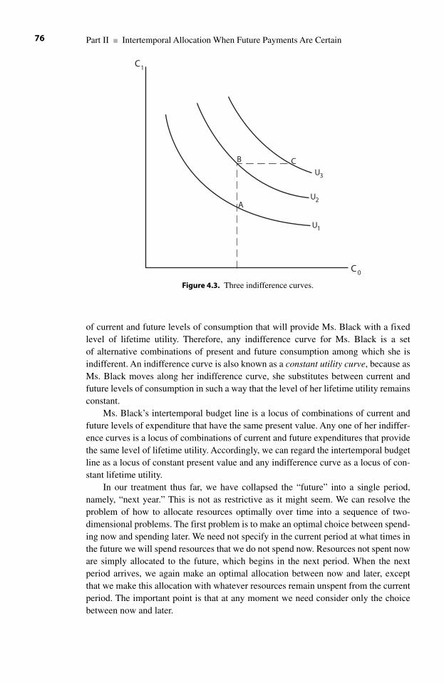
of current and future levels of consumption that will provide Ms. Black with a fixedlevel of lifetime utility. Therefore, any indifference curve for Ms. Black is a set of alternative combinations of present and future consumption among which she isindifferent. An indifference curve is also known as a constant utility curve, because asMs. Black moves along her indifference curve, she substitutes between current andfuture levels of consumption in such a way that the level of her lifetime utility remainsconstant.

Ms. Black’s intertemporal budget line is a locus of combinations of current andfuture levels of expenditure that have the same present value. Any one of her indiffer-ence curves is a locus of combinations of current and future expenditures that providethe same level of lifetime utility. Accordingly, we can regard the intertemporal budgetline as a locus of constant present value and any indifference curve as a locus of con-stant lifetime utility.

In our treatment thus far, we have collapsed the “future” into a single period,namely, “next year.” This is not as restrictive as it might seem. We can resolve theproblem of how to allocate resources optimally over time into a sequence of two-dimensional problems. The first problem is to make an optimal choice between spend-ing now and spending later. We need not specify in the current period at what times inthe future we will spend resources that we do not spend now. Resources not spent noware simply allocated to the future, which begins in the next period. When the nextperiod arrives, we again make an optimal allocation between now and later, exceptthat we make this allocation with whatever resources remain unspent from the currentperiod. The important point is that at any moment we need consider only the choicebetween now and later.


C 0

C1

CB

A

U1

U2

U3

Figure 4.3. Three indifference curves.

4.2.1 Postulates That Govern Indifference Curves

Each of the three indifference curves in figure 4.3 corresponds to a specified, constantlevel of utility for Ms. Black. Let U1, U2, and U3 denote the three levels of utility, anddesignate each indifference curve according to its level of utility. Economists use a setof postulates (or assumptions) to characterize the preferences of a typical consumer.These postulates are sufficiently plausible so that economists are willing to use themto construct theoretical models. More important, the models that are built on thesepostulates are quite successful in generating empirically verified predictions. That is,the postulates work; by using the postulates, economists can discover importantinsights into how consumers make choices. These postulates apply quite generally tothe preferences of a typical consumer, not just to those preferences that involveintertemporal allocation. We will now use these postulates to justify the features of theindifference curves in figure 4.3.

One of the postulates states that a consumer is willing to substitute less of onegood for a sufficiently large increase in another good. Willing to substitute means thatthe effect on the consumer’s utility of the increase in her quantity of one good isexactly offset by the decrease in her quantity of the other good. In our case, the twogoods are the levels of current and future consumption. The postulate states that for asufficient increase in current consumption, the consumer is willing to forego somequantity of future consumption; the converse is also true. The willingness of a con-sumer to substitute between any Good X and any Good Y implies that an indifferencecurve for these two goods will have a negative slope.

A second postulate states that a consumer will gain utility if she acquires more ofany good without decreasing the quantity of any other good that she has. This postu-late is often known as “more is better than less.” In figure 4.3, none of the three curvesintersects with any other curve. Therefore, any two curves correspond to different lev-els of utility. Furthermore, if one curve lies above and to the right of a second curve,the first curve will correspond to the higher level of utility. This means that the threelevels of utility satisfy the relationship U1U2U3. Consider the points A, B, and Cin figure 4.3. Points A and B provide the same level of current consumption and differ-ent levels of future consumption. Similarly, points B and C provide the same level offuture consumption and different levels of current consumption. The postulate thatmore is better than less implies that the consumer’s level of utility at point C is greaterthan her utility at point B, which in turn is greater than her utility at point A. Moregenerally, the consumer’s levels of utility increase as she moves rightward from indifference curve U1 to indifference curve U2 to indifference curve U3.

We can use a third postulate to justify the convex shape of an indifference curve.This third postulate states that the rate at which Ms. Black is willing to forego futureconsumption in exchange for a one-unit increase in current consumption diminishesas she moves downward and rightward along any of her indifference curves. The rateat which Ms. Black is willing to substitute between current and future consumption isequal to the slope of the straight line that is tangential to an indifference curve at thepoint that corresponds to her present levels of current and future consumption.Clearly, the (absolute values of the) slopes of these tangential lines diminish as theconsumer moves downward and rightward along any one of the indifference curves.


Mathematicians define as convex a curve that has the shape of the indifference curvesin figure 4.3.2

Economists use postulates to construct models of economic phenomena. Thevalue of a model is its ability to clarify thinking and to generate empirically verifiedhypotheses. By extension, a set of postulates is valuable if economists can build valu-able models based on those postulates. We will not attempt to prove here that an indi-vidual’s indifference curves are convex. We do offer the following example as aplausible rationale for this postulate.

Consider Mr. and Mrs. Saratoga, who enjoy dining in a certain class of restaurantwith their two sons and their daughter. The cost of a typical meal for this family in theserestaurants is $80. As a result, each time the Saratogas go to one of these restaurants,they must forego $80 worth of other goods and services that they could have purchasedelsewhere. (Since this is a text on the economics of financial markets, it is important torecognize that among the goods that the Saratogas could have purchased are financialsecurities. That is, the Saratogas could have “saved” the $80, or any portion of it, bypurchasing financial securities.) The question that arises from this situation is: how fre-quently per month will the Saratogas dine out if the cost of a meal is $80?

We can appreciate the implications of convexity of indifference curves if werestate the preceding question in the form of a marginal rate of substitution, as fol-lows: How much spending on other goods and services will the Saratogas forego toincrease by one the number of times per month that they dine in the restaurant? Thepostulate that indifference curves are convex implies that the amount of spending onalternatives that the Saratogas are willing to forego diminishes as the number of occa-sions on which they dine out per month increases.

For example, the family might be willing to pay at most $110 for the opportunity todine out three times per month rather than two times per month. But the Saratogas arewilling to pay at most $90 to dine out four times per month rather than three. Convexityof their indifference curves means that the marginal values of these occasions diminishas their frequency per month increases. Since the cost of each meal is $80, the Saratogaswill dine out at least four times per month. In fact, this family will increase the fre-quency with which they dine out until the amount of spending on other goods that theyare willing to forego decreases below $80. In technical language, the convexity of theirindifference curves means that the marginal rate at which the Saratogas are willing tosubstitute away from other goods diminishes as the frequency of dining out increases.

4.2.2 The Marginal Rate of Intertemporal Substitution

Consider point D on indifference curve U1 in figure 4.4. In a small neighborhood ofpoint D, we can approximate movements along the indifference curve by movementsalong the straight line that is tangential to the indifference curve at point D. Designatethis line as line D. Suppose that the slope of line D is (�)4:1. If Ms. Black is now atpoint D, then the maximal amount of future consumption that she can forego inexchange for an increase of $1 in current consumption without suffering a reduction inher level of utility is $4. If Ms. Black could obtain an increase of $1 in current con-sumption while giving up less than $4 in future consumption, she would obtain a netincrease in her level of utility.


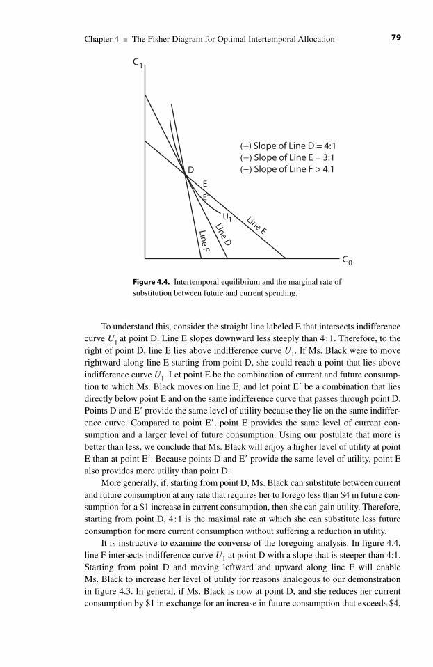
To understand this, consider the straight line labeled E that intersects indifferencecurve U1 at point D. Line E slopes downward less steeply than 4:1. Therefore, to theright of point D, line E lies above indifference curve U1. If Ms. Black were to moverightward along line E starting from point D, she could reach a point that lies aboveindifference curve U1. Let point E be the combination of current and future consump-tion to which Ms. Black moves on line E, and let point E be a combination that liesdirectly below point E and on the same indifference curve that passes through point D.Points D and E provide the same level of utility because they lie on the same indiffer-ence curve. Compared to point E, point E provides the same level of current con-sumption and a larger level of future consumption. Using our postulate that more isbetter than less, we conclude that Ms. Black will enjoy a higher level of utility at pointE than at point E. Because points D and E provide the same level of utility, point Ealso provides more utility than point D.

More generally, if, starting from point D, Ms. Black can substitute between currentand future consumption at any rate that requires her to forego less than $4 in future con-sumption for a $1 increase in current consumption, then she can gain utility. Therefore,starting from point D, 4:1 is the maximal rate at which she can substitute less futureconsumption for more current consumption without suffering a reduction in utility.

It is instructive to examine the converse of the foregoing analysis. In figure 4.4,line F intersects indifference curve U1 at point D with a slope that is steeper than 4:1.Starting from point D and moving leftward and upward along line F will enable Ms. Black to increase her level of utility for reasons analogous to our demonstration in figure 4.3. In general, if Ms. Black is now at point D, and she reduces her currentconsumption by $1 in exchange for an increase in future consumption that exceeds $4,


C0

C1

E’

E

D

Line E

LineD

Line

F

(−) Slope of Line D = 4: 1(−) Slope of Line E = 3:1(−) Slope of Line F > 4:1

U1

Figure 4.4. Intertemporal equilibrium and the marginal rate ofsubstitution between future and current spending.

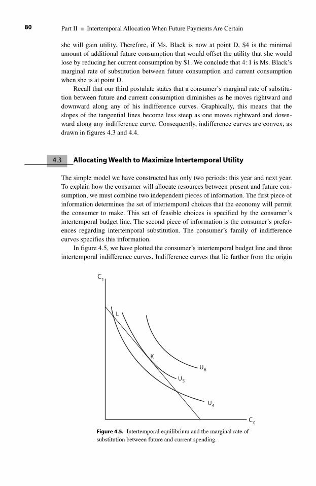
she will gain utility. Therefore, if Ms. Black is now at point D, $4 is the minimalamount of additional future consumption that would offset the utility that she wouldlose by reducing her current consumption by $1. We conclude that 4:1 is Ms. Black’smarginal rate of substitution between future consumption and current consumptionwhen she is at point D.

Recall that our third postulate states that a consumer’s marginal rate of substitu-tion between future and current consumption diminishes as he moves rightward anddownward along any of his indifference curves. Graphically, this means that theslopes of the tangential lines become less steep as one moves rightward and down-ward along any indifference curve. Consequently, indifference curves are convex, asdrawn in figures 4.3 and 4.4.

4.3 Allocating Wealth to Maximize Intertemporal Utility

The simple model we have constructed has only two periods: this year and next year.To explain how the consumer will allocate resources between present and future con-sumption, we must combine two independent pieces of information. The first piece ofinformation determines the set of intertemporal choices that the economy will permitthe consumer to make. This set of feasible choices is specified by the consumer’sintertemporal budget line. The second piece of information is the consumer’s prefer-ences regarding intertemporal substitution. The consumer’s family of indifferencecurves specifies this information.

In figure 4.5, we have plotted the consumer’s intertemporal budget line and threeintertemporal indifference curves. Indifference curves that lie farther from the origin


C0

C1

L

K

U4

U5

U6

Figure 4.5. Intertemporal equilibrium and the marginal rate ofsubstitution between future and current spending.

correspond to higher levels of utility. But the consumer can reach only those indifference curves that contain points that lie on or below the budget line. Since herindifference curves are convex, the highest curve that she can reach will be the curvethat is tangential to the budget line. This curve, and its point of tangency with thebudget line, will be unique because all of the indifference curves are convex and thebudget line is linear.

The intertemporal budget line is a frontier that defines the maximal level of futureconsumption that the individual can afford, given her level of current consumptionand level of wealth. Clearly, the individual would not choose a combination of currentand future consumption levels that plot below her intertemporal budget line. Startingfrom any position below the budget line, an individual could increase her level of current consumption without foregoing any future consumption. She could alsoincrease her level of future consumption without foregoing any current consumption.Moreover, she could increase both current and future consumption. We assume thatthe individual will not forego an opportunity to increase her level of consumption inone dimension if there is no cost in terms of a decrease in her level of consumption inanother dimension. Therefore, an individual will always choose a position on, and notbelow, her intertemporal budget line.

Let the point of tangency be at K on indifference curve U5 in figure 4.5. Then theslope of indifference curve U5 at point K is equal to the (constant) slope of the budgetline. Therefore, to maximize her lifetime utility, the consumer will choose thesequence of current and future consumption that lies on her budget line at a pointwhere the rate at which she is willing to substitute between current and future con-sumption is equal to the rate at which the market will allow her to substitute by meansof either borrowing or lending. Equating these two rates of substitution is an essentialcondition that the consumer must meet if she is to maximize her lifetime utility. Wecan appreciate this more fully by considering an allocation in which the consumer hasnot satisfied this condition.

Consider point L on the budget line in figure 4.5. Every point in the quadrant has precisely one indifference curve passing through it. Since the indifference curves are con-vex, and since indifference curve U5 is tangential to the budget line at point K, that indif-ference curve cannot pass through L. Let U4 be the indifference curve that passes throughL. Then indifference curve U4 must be lower than indifference curve U5, and it mustintersect the budget line at point L. Since the slope of the indifference curve is steeperthan the slope of the budget line at point L, Ms. Black is willing to forego more in futureconsumption to obtain one more dollar in current consumption than the market requires.

For example, suppose that the slope of the indifference curve at point L is (�)6:1,and the slope of the budget line is (�)2:1. If Ms. Black has allocated her resources sothat her sequence of current and future consumption is at L, then she is not maximiz-ing her lifetime utility. Here is the reason: the market will allow Ms. Black to borrow$1 today if she will repay $2 next year. But at point L she is willing to repay as muchas $6 next year if she can borrow $1 today. Clearly, Ms. Black should borrow. By bor-rowing, she can move rightward and downward along her budget line and thus moveto a higher indifference curve.

We conclude that to maximize her lifetime utility, Ms. Black must allocate herresources so that the rate at which she is willing to substitute less future consumption


for an extra $1 of current consumption is equal to the rate at which the market willallow her to do so.

We can put this conclusion another way. At point L, Ms. Black’s marginal valueof an additional $1 of current consumption exceeds her marginal cost. Both marginalvalue and marginal cost are measured in terms of the amount of future consumptionforegone.

4.4 Mutually Beneficial Exchanges

In the preceding subsection, we determined how Ms. Black should allocate herresources if she can borrow or lend. Of course, Ms. Black does not lend to or borrowfrom the market. Rather, the market is a conduit through which Ms. Black can conductmutually beneficial exchanges with other consumers. This market will be economi-cally efficient if it enables consumers to identify and effect all the possibilities formutually beneficial exchanges. We will examine this property of economic efficiencyby considering two consumers, Ms. Black and Mr. Green. In what follows, we assumethat these are typical of a large number of consumers, each of whom is too small toaffect the interest rate at which they can borrow or lend. That is, we assume that themarket is perfectly competitive.

Competition among consumers who want to maximize lifetime utility by borrow-ing or lending determines an equilibrium rate of interest, which in turn determines theslope of each consumer’s intertemporal budget line. Since the market is perfectlycompetitive, every consumer will face the same interest rate. Consequently, everyconsumer’s intertemporal budget line will have the same slope, namely �(1�r). Thefact that all consumers face the same interest rate is critical for showing that the mar-ket for borrowing and lending is economically efficient.

Although Ms. Black and Mr. Green face the same interest rate, these two con-sumers differ in two respects. First, the two persons have different levels of wealth.Their intertemporal budget lines lie at different distances from the origin. Second, thetwo persons have different preferences regarding substitution between current andfuture consumption. Therefore, Ms. Black’s set of indifference curves will not havethe same shapes as Mr. Green’s indifference curves.

In figure 4.6 (a) and (b), we have drawn the budget lines and indifference curvesfor the two consumers. Ms. Black’s sequence of income payments is located at pointT in figure 4.6(a). She has a relatively small current income and a relatively largefuture income. Mr. Green has the opposite configuration of current and futureincomes; his sequence of income payments lies at point Q in figure 4.6(b). Theintertemporal budget line for each consumer is a straight line that passes through thatconsumer’s income sequence and has a slope equal to �(1�r). Ms. Black is wealthierthan Mr. Green because her budget line lies farther out from the origin. If we were toplot both budget lines on the same graph, Mr. Green’s budget line would lie betweenthe origin and Ms. Black’s budget line. Consequently, Ms. Black can afford any of thecombinations of current and future consumption that Mr. Green can afford, and manycombinations that he cannot afford; Mr. Green can afford only a subset of the combi-nations that Ms. Black can afford.


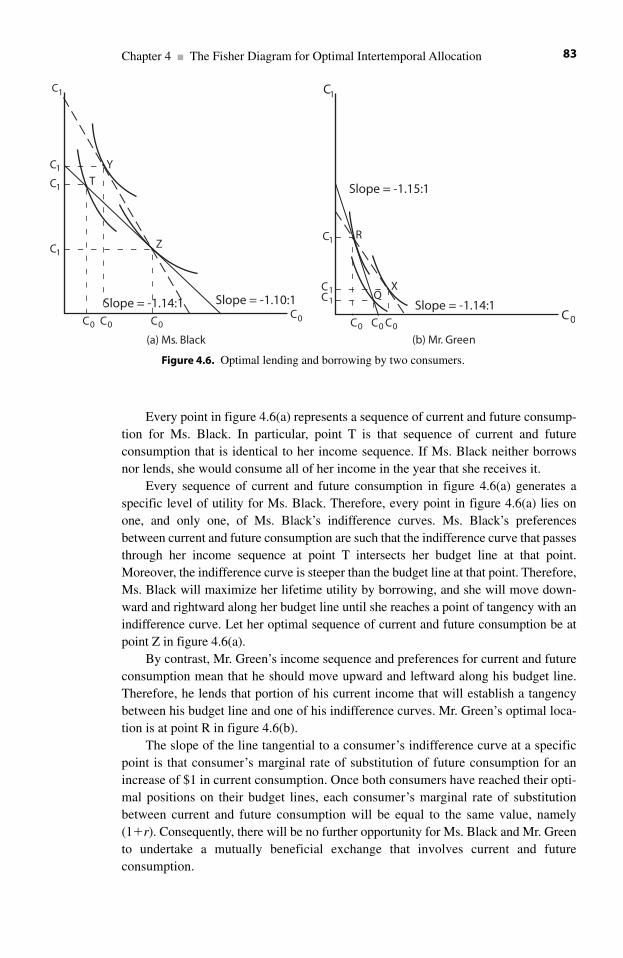
Every point in figure 4.6(a) represents a sequence of current and future consump-tion for Ms. Black. In particular, point T is that sequence of current and future consumption that is identical to her income sequence. If Ms. Black neither borrowsnor lends, she would consume all of her income in the year that she receives it.

Every sequence of current and future consumption in figure 4.6(a) generates a specific level of utility for Ms. Black. Therefore, every point in figure 4.6(a) lies onone, and only one, of Ms. Black’s indifference curves. Ms. Black’s preferencesbetween current and future consumption are such that the indifference curve that passesthrough her income sequence at point T intersects her budget line at that point.Moreover, the indifference curve is steeper than the budget line at that point. Therefore,Ms. Black will maximize her lifetime utility by borrowing, and she will move down-ward and rightward along her budget line until she reaches a point of tangency with anindifference curve. Let her optimal sequence of current and future consumption be atpoint Z in figure 4.6(a).

By contrast, Mr. Green’s income sequence and preferences for current and futureconsumption mean that he should move upward and leftward along his budget line.Therefore, he lends that portion of his current income that will establish a tangencybetween his budget line and one of his indifference curves. Mr. Green’s optimal loca-tion is at point R in figure 4.6(b).

The slope of the line tangential to a consumer’s indifference curve at a specificpoint is that consumer’s marginal rate of substitution of future consumption for anincrease of $1 in current consumption. Once both consumers have reached their opti-mal positions on their budget lines, each consumer’s marginal rate of substitutionbetween current and future consumption will be equal to the same value, namely(1�r). Consequently, there will be no further opportunity for Ms. Black and Mr. Greento undertake a mutually beneficial exchange that involves current and future consumption.


C0C0C0C0

C1

C1

C1

T

Z

Slope = -1.10:1Slope = -1.14:1

Y

(a) Ms. Black

C0

C1C1

(b) Mr. Green

C0C0C0

C1C1

C1

QX

Slope = -1.15:1

Slope = -1.14:1

R

Figure 4.6. Optimal lending and borrowing by two consumers.

To verify this last statement, suppose that Ms. Black faces an interest rate equal to .10 (per year), while Mr. Green faces an interest rate equal to .15. Then the budgetlines for the two consumers would have different slopes. By reducing her consumptionthis year by $100, Ms. Black could increase her consumption next year by $110. But Mr. Green could increase his consumption next year by $115 if he reduced his con-sumption this year by $100. To maximize her utility, Ms. Black would choose a loca-tion along her budget line at which her marginal rate of substitution is equal to(1�.10):1. That is, once Ms. Black has allocated her resources optimally between cur-rent and future consumption, she will be willing to give up no more than $1.10 in futureconsumption in exchange for an additional $1.00 in current consumption. Conversely,Ms. Black would require at least $1.10 in additional future consumption in exchangefor giving up $1.00 in current consumption.

Similarly, Mr. Green would choose a position along his budget line at which hismarginal rate of substitution is equal to (1�.15) :1.

There would now be a potential for a mutually beneficial exchange between thetwo consumers. Mr. Green would have a higher marginal value of current consump-tion, measured in terms of future consumption foregone, than would Ms. Black. Thus,both consumers could increase their levels of utility if Mr. Green were to borrow fromMs. Black.

Suppose that Mr. Green proposed to borrow from Ms. Black at an interest rateequal to .14. That is, Mr. Green would borrow $1.00 from Ms. Black today and repayher $1.14 next year. Mr. Green would gain utility because he would be willing to payas much as $1.15 next year if he could increase his current consumption by $1.00.Similarly, Ms. Black would gain utility because she would be willing to reduce hercurrent consumption by $1.00 in exchange for as little as $1.10 in additional consump-tion next year.

In figure 4.6(b), we show how Mr. Green could increase his utility by borrowingfrom Ms. Black. If he had no opportunity to borrow from Ms. Black, Mr. Greenwould be constrained to the choices represented by his budget line. Under this con-straint, he would maximize his utility by locating his consumption sequence at pointR, where his indifference curve is tangential to his budget line. Since the slope of hisbudget line is equal to �(1�.15), the slope of his indifference curve at point R wouldalso be equal to �(1�.15). If Mr. Green could now borrow $1.00 and repay only$1.14 next year, he would move to a higher indifference curve. By paying interest ata rate equal to .14, he would move along a straight line whose slope is less steep thanthe slope of his budget line. That is, the straight line that represents his opportunitiesto borrow from Ms. Black would intersect his budget line at point R and would moveabove that budget line to the right of point R. Therefore, by borrowing from Ms. Black, Mr. Green could move to a higher indifference curve and maximize utility at point X.

In figure 4.6(a), we show in an analogous way that Ms. Black could move to ahigher indifference curve by lending to Mr. Green. If she had no opportunity to lend toMr. Green, Ms. Black would be constrained to a budget line whose slope is equal to�(1�.10). Suppose that, under this constraint, she chose point Z on her budget line.The slope of her indifference curve at this point would be equal to �(1�.10). If shecould now lend to Mr. Green at an interest rate equal to .14, she could move upward


and leftward from point Z along a straight line whose slope is equal to �(1�.14). Thisstraight line is steeper than her budget line. Therefore, by lending to Mr. Green, Ms. Black could move to a higher indifference curve; she would thus maximize utilityby locating her consumption sequence at point Y, the point of tangency between hernew indifference curve and new budget line.

We draw two conclusions. First, unless every consumer faces the same interestrate, there will be unrealized opportunities for mutually beneficial intertemporalexchanges. Second, if all consumers face the same interest rate, r, and maximize util-ity, then (1�r) is the common marginal rate of substitution at which any consumer iswilling to forego future consumption in exchange for a $1.00 increase in current con-sumption. Equivalently, (1�r) is the common minimal increase in future consumptionthat every consumer will require as compensation for reducing current consumptionby $1.00. This relationship between the interest rate and the rate at which consumerswill substitute between current and future consumption is critical for determining therate at which the economy should accumulate capital if consumers are to maximizetheir levels of lifetime utility. We consider the question of efficiency in the accumula-tion of capital in the next section.

4.5 The Efficient Level of Investment

We recall from chapter 1 that consumers can increase their stock of capital goods bydiverting resources away from the production of consumption goods. This exchangeof consumption goods for capital goods is called an investment.

By investing in one year, consumers can enjoy a larger volume of consumptiongoods in future years than would be possible without the investment. Therefore, aninvestment is an exchange of current consumption goods for an increase in the quan-tity of future consumption goods.

There is sometimes confusion between lending and investment. Borrowing andlending are obviously opposite sides of the same transaction. Whether an investmentis made depends on whether or not the borrower uses the borrowed resources to con-struct capital goods. If she does, then the lender has financed investment by decreas-ing his current consumption. But if the borrower uses the resources to increase herown level of current consumption above her current income, there is no investmentbecause there is no increase in the stock of capital goods. The lender and the borrowerwill simply have exchanged portions of their current and future levels of consumption.

To what extent will consumers invest? How do financial markets contribute toreaching an economically efficient resolution of the allocation of resources betweencurrent and future consumption? We can use the analysis of the preceding subsectionto answer these questions.

We know that if a consumer can borrow or lend, she will move along her budgetline until she establishes a tangency between that budget line and one of her indiffer-ence curves. At this point of tangency, her marginal rate of substitution of future con-sumption for an extra $1.00 of current consumption will be equal to (1�r) :1, if r isthe rate of interest at which that consumer can borrow or lend. If every consumer faces


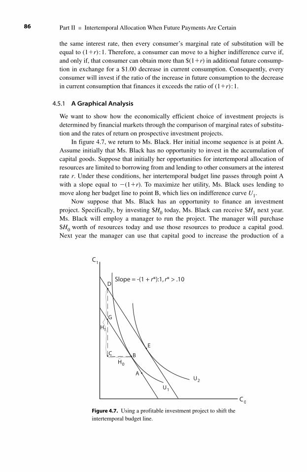
the same interest rate, then every consumer’s marginal rate of substitution will beequal to (1�r) :1. Therefore, a consumer can move to a higher indifference curve if,and only if, that consumer can obtain more than $(1�r) in additional future consump-tion in exchange for a $1.00 decrease in current consumption. Consequently, everyconsumer will invest if the ratio of the increase in future consumption to the decreasein current consumption that finances it exceeds the ratio of (1�r) :1.

4.5.1 A Graphical Analysis

We want to show how the economically efficient choice of investment projects isdetermined by financial markets through the comparison of marginal rates of substitu-tion and the rates of return on prospective investment projects.

In figure 4.7, we return to Ms. Black. Her initial income sequence is at point A.Assume initially that Ms. Black has no opportunity to invest in the accumulation ofcapital goods. Suppose that initially her opportunities for intertemporal allocation ofresources are limited to borrowing from and lending to other consumers at the interestrate r. Under these conditions, her intertemporal budget line passes through point Awith a slope equal to �(1�r). To maximize her utility, Ms. Black uses lending tomove along her budget line to point B, which lies on indifference curve U1.

Now suppose that Ms. Black has an opportunity to finance an investment project. Specifically, by investing $H0 today, Ms. Black can receive $H1 next year.Ms. Black will employ a manager to run the project. The manager will purchase $H0 worth of resources today and use those resources to produce a capital good. Next year the manager can use that capital good to increase the production of a


C 0

U2

U1

Slope = -(1 + r*):1, r* > .10

C1

D

E

H1

A

G

C BH0

Figure 4.7. Using a profitable investment project to shift theintertemporal budget line.

consumption good, which he can sell for $H1. Assume that the manager’s wage isincluded in $H0 and that the capital good lasts only one year. Then the full cost of theproject is $H0, and the full benefit is $H1. Ms. Black incurs the cost in the form of adecrease in her consumption this year; she receives the benefit as an increase in herconsumption next year.

Should Ms. Black undertake this project? If so, how should she finance it? If theratio of $H1 to $H0 exceeds (1�r), the answer is yes, because the project will enableMs. Black to reach a higher indifference curve than the one that she currently occu-pies. If future payments are known with certainty, which is the assumption throughoutthis chapter, then the method that Ms. Black uses to finance the project will have noeffect on the size of her gain from the project. This assertion follows from a consider-ation of opportunity costs.

Suppose that the ratio of $H1 to $H0 exceeds (1�r), so that Ms. Black shouldundertake the project. In figure 4.7, we have shown the cost of the project, $H0, as aleftward movement from point B to point C. That is, Ms. Black finances the project byreducing her current consumption by the amount $H0. The payoff from the project is$H1, which we show as a vertical movement from point C to point D. By financing theproject, Ms. Black moves from point B in the current year to point D in the next year.Since the ratio of $H1 to $H0 exceeds (1�r), a straight line drawn between points Band D would be steeper than Ms. Black’s budget line. Consequently, by financing theproject she can reach a combination of current and future consumption that lies abovethe budget line that passes through her initial income sequence.

Investing in the project enables Ms. Black to reach the higher budget line thatpasses through point D. This budget line is parallel to her original budget linebecause the interest rate at which she can borrow or lend is still r. Therefore, onceMs. Black reaches point D on the higher budget line, she can borrow or lend her wayto any other point on that line. Clearly, if Ms. Black can move to any point on thehigher of the two budget lines, she can reach a higher indifference curve by investingin the project. The optimal point for Ms. Black on the higher indifference curve is, ofcourse, point E, the point of tangency between the budget line and one of her indif-ference curves.

In drawing figure 4.7, we have assumed that Ms. Black’s preferences regardingcurrent and future consumption are such that this point of tangency on the higherbudget line lies at point E, which is upward and rightward from the tangency at point Bon her initial budget line. In this event, Ms. Black would maximize her utility by usingthe project to increase both her current and her future consumption. We need not haveplaced point E upward and rightward from point A. If the project has a positive netpresent value, then the ratio of H1/H0 will exceed (1�.10 )/1. If this condition is satis-fied, Ms. Black can use an investment in the project to reach a higher budget line thanthe line on which her initial sequence of income lies. Once on the higher budget line,she can use borrowing or lending to move along that line to a point of tangency withan indifference curve. The indifference curve that is tangential to the higher budgetline necessarily represents a higher level of utility than the indifference curve that istangential to the lower budget line. Therefore, investing in the project enables Ms. Blackto increase her level of utility.3


4.5.2 Profit versus Utility

The conclusion in the preceding section bears further discussion. Some will argue thatwhile a project is “profitable,” consumers will not finance the project because itrequires too large a reduction in current consumption. This argument is incorrectbecause it confuses profit with utility. The configuration of Ms. Black’s indifferencecurves in figure 4.7 illustrates why this argument fails.

Since the ratio H1/H0 exceeds (1�.10) :1, the project is profitable. We can iden-tify the profit either as a payoff in dollars or as a rate of return.

Profit in Terms of Dollars

We first demonstrate that the payoff in dollars exceeds the opportunity cost. Tofinance the project, Ms. Black must reduce her current consumption by H0, which isthe horizontal distance between points B and D in figure 4.7. If Ms. Black invested$H0 in a bank today, next year she would have (including both principal and interest)an amount of money equal to the vertical distance between points B and G. But if sheinvests H0 in the project today, her payoff next year will be the vertical distancebetween points B and D. Since point D is vertically above point G, the project morethan covers Ms. Black’s opportunity costs and is therefore profitable. Its payoff in dol-lars exceeds what Ms. Black could obtain from investing in a bank account.

Profit in Terms of Rate of Return

We can restate the preceding analysis by examining the rate of return on the project,rather than calculating the amount of the payoff in dollars. The rate of return on theproject exceeds the rate of return at the bank. Investing in the project allows Ms. Blackto move from point B to point D in figure 4.7. The slope of the straight line connect-ing these points is steeper than the original budget line. The slope of the budget line is�(1�r) :1. Let the slope of a line connecting points B and D be �(1�r*):1. Then r*must exceed r. The project takes Ms. Black from point B to point D by generating arate of return that exceeds the rate of return that she can get in a bank. That is, the proj-ect is profitable because its rate of return exceeds Ms. Black’s opportunity cost.

A Numerical Example

Let the points B, G, and D in figure 4.7 have the following coordinates:

B�{B0, B1}�{$400, $700}

G�{G0, G1}�{$300, $810}

D�{D0, D1}�{$300, $860}

Let the interest rate, r, be .10 per year.Points B, G, and D represent alternative sequences of payments. The horizontal

distance between point B and point G, and between point B and point D, is $100. Thevertical distance between point B and point G is $110. The vertical distance betweenpoint B and point D is $160.


Since points B and G lie on the same budget line, their sequences have the samepresent value. Since point D is vertically above point G, the project more than coversMs. Black’s opportunity costs and is therefore profitable. Since the interest rate is .10per year, the slope of a budget line is �(1�.10) :1, which is the rate at whichMs. Black can substitute between consumption next year and consumption this year.For example, if Ms. Black were at point B, she could move to point G by reducing hercurrent consumption by $100 and investing that amount in a bank. Next year, herincome will be $700 plus the $110 that she can withdraw from the bank. She couldthen consume next year at a level of $700�$110�$810. The net return on her invest-ment would be ($110�$100)/$100�.10.

Instead of investing $100 in a bank, Ms. Black could invest in the project. To do thiswould be to move from point B to point D in figure 4.7. Next year her payoff from theproject will be $160. Combining this payoff with the income of $700 that she willreceive next year independently of the project, she could consume next year at a level of$700�$160, or $860. The net return on her investment would be ($160�$100)/$100, or.60. The slope of a straight line connecting points B and D would be �(1�.60):1.

We have established that the project is profitable, whether we measure profit interms of dollars or in terms of rate of return. Now consider whether the project canenable Ms. Black to increase her utility.

In figure 4.7, point D lies below indifference curve U1, which is the highest indif-ference curve that she could reach on her initial budget line. Therefore, Ms. Black willhave less utility if she undertakes the project and moves to point D than she will haveif she remains at point B. The project does not provide Ms. Black with a sufficientincrease in future consumption to compensate her for the decrease in current con-sumption required to finance the project; therefore, Ms. Black will not finance theproject.

But this argument ignores the fact that if Ms. Black has access to a financial mar-ket in which she can borrow and lend, she need not reduce her current consumption atall in order to finance the project. In fact, depending on her preferences for current andfuture consumption, she gains utility by financing the project and increasing her cur-rent consumption.

In figure 4.8, we demonstrate how Ms. Black could use an investment in theproject to move directly from her initial income sequence to her optimal sequence ofcurrent and future consumption.

Ms. Black’s initial income sequence is at point A. Then her initial budget linepasses through point A with a slope equal to �(1�.10):1. The project requires aninvestment of H0 dollars today and generates a return of H1 dollars next year. The ratioH1/H0 � (1�.10):1. We can represent the project graphically by starting at any point onMs. Black’s initial budget line, moving leftward by a distance of H0 and then upward bya distance of H1. Starting from point A, Ms. Black could borrow the amount (E0�Z0).By construction, (E0�Z0)�(E0�A0)�(A0�Z0), and (A0�Z0)�H0, which is theamount by which Ms. Black must reduce her current spending to finance the project.

Ms. Black could use the (E0�Z0) that she borrows in the current year to financethe project, H0�(A0�Z0), and increase her spending on current consumption by theamount (E0�A0). Next year, Ms. Black’s income will be Z1, which is the sum of A1,which she will receive independently of the project, plus the payoff, H1�(Z1�A1),


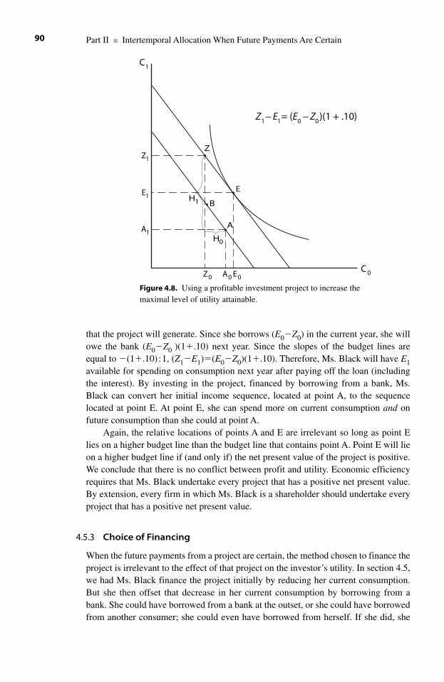
that the project will generate. Since she borrows (E0�Z0) in the current year, she willowe the bank (E0�Z0 )(1�.10) next year. Since the slopes of the budget lines areequal to �(1�.10) :1, (Z1�E1)�(E0�Z0)(1�.10). Therefore, Ms. Black will have E1available for spending on consumption next year after paying off the loan (includingthe interest). By investing in the project, financed by borrowing from a bank, Ms.Black can convert her initial income sequence, located at point A, to the sequencelocated at point E. At point E, she can spend more on current consumption and onfuture consumption than she could at point A.

Again, the relative locations of points A and E are irrelevant so long as point Elies on a higher budget line than the budget line that contains point A. Point E will lieon a higher budget line if (and only if) the net present value of the project is positive.We conclude that there is no conflict between profit and utility. Economic efficiencyrequires that Ms. Black undertake every project that has a positive net present value.By extension, every firm in which Ms. Black is a shareholder should undertake everyproject that has a positive net present value.

4.5.3 Choice of Financing

When the future payments from a project are certain, the method chosen to finance theproject is irrelevant to the effect of that project on the investor’s utility. In section 4.5,we had Ms. Black finance the project initially by reducing her current consumption.But she then offset that decrease in her current consumption by borrowing from abank. She could have borrowed from a bank at the outset, or she could have borrowedfrom another consumer; she could even have borrowed from herself. If she did, she


E0

E1

A0

A1

Z0

Z1− E 1 = (E0 − Z 0 )(1 + .10)

Z1

Z

EH1

A

B

H0

C 0

C1

Figure 4.8. Using a profitable investment project to increase themaximal level of utility attainable.

would have incurred an implicit cost in the form of interest foregone. If she chooses toborrow from a bank or from someone else, she will incur an explicit cost in the formof the interest that she pays. Examining figure 4.7 will show that the indifferencecurve that Ms. Black can reach by investing in the project does not depend on herchoice of how to finance the project.

We can easily demonstrate the foregoing result numerically in chapter 5, wherewe consider firms explicitly. In chapter 13 we will show that if future payments arenot certain, the choice of the method of financing does have an effect on whether ornot investors can gain utility by undertaking the project.

4.5.4 Summary of Efficient Investment

To achieve an efficient allocation of resources, consumers should finance all projectswhose (net) rates of return r* exceed the rate of interest r. Equivalently, consumersshould finance all projects that are profitable in the sense that the (net) rate of return r*on the funds invested exceeds the opportunity cost r incurred by not depositing thosefunds in a bank. This correspondence between maximizing profit and maximizingutility is a central principle in economics. We are not saying that profit and utility areidentical; indeed, a person’s utility usually depends on many considerations in addi-tion to income, profit, or (monetary) wealth. We are saying that in a financial market,the allocation of resources that will maximize a person’s profit is the same allocationthat will maximize his or her utility.

At any moment, there will be several potential investment projects. We could rankthese projects in descending order by the values of their rates of return. We know thatconsumers should finance all projects whose rates of return exceed the interest rate, r.Suppose that consumers begin to finance projects, choosing first the project that has thehighest rate of return, and choosing additional projects in descending order of their ratesof return. As consumers accept more projects, they increase the extent to which they areforegoing current consumption in exchange for increases in future consumption. Byanalogy to the argument in the preceding subsection, the convexity of indifferencecurves means that the common value of consumers’ marginal rates of substitution willincrease as consumers trade away more and more current consumption. This increase inthe common value of the marginal rate of substitution will increase the equilibriumvalue of the interest rate, r. Thus, as more and more projects are undertaken, the rate ofreturn of the marginal project will decrease, and the common value of the marginal rateof substitution will increase. The market will reach an equilibrium when the value of theinterest rate and the value of the common marginal rate of substitution are equal.

4.6 The Importance of Informational Efficiency in the Prices of Financial Securities

We know that economic efficiency requires that individuals undertake all mutuallybeneficial exchanges. We also know that in a society that has both a large populationand access to complex technologies, there are substantial costs in identifying andeffecting all the possibilities for mutually beneficial exchanges. An essential function


of a system of financial markets is to transmit information about investment projectsand about the rates at which investors are willing to substitute present and future con-sumption. We say that a financial market is informationally efficient if the prices offinancial securities contain all the information that investors need to identify andundertake all mutually beneficial exchanges.

If Ms. Black and Mr. Green are willing to substitute between present and futureconsumption at different (marginal) rates, they can effect a mutually beneficialexchange. In a modern economy, they would transmit information about their rates ofsubstitution by the prices at which they are willing to buy or sell financial securities.But to achieve economic efficiency, these prices must accurately reflect marginal ratesof substitution. If the prices do not do this, some potentially mutually beneficialexchanges will be foregone.

As another example, suppose that a firm has a project that will generate a rate ofreturn equal to 16% per year. Prospective investors are willing to lend at 10% per year.If the investors can inspect the project and determine for themselves that it will pay16%, then the firm (acting as an agent for current shareholders) and the new investorscan create a mutually beneficial exchange. In a modern economy, the technologicalcomplexity and the scale of most projects precludes firms from raising the requisitefinancing from investors who will examine the plans for the project at the same levelof detail as the firms have done. Rather, firms and investors will rely on the prices offinancial securities to transmit information about proposed investment projects andabout the willingness of investors to finance those projects. If the prices of securitiesdo not transmit sufficient information about these projects, there will be an inefficientallocation of resources because some mutually beneficial exchanges will be foregone.

In some situations, a firm can transmit information about investment projectsonly by the firm’s choice of which kind of security to offer to new investors. Webriefly discussed an example of this in chapter 2 when we asserted that a firm couldovercome a problem of asymmetric information by offering a convertible bond, ratherthan a straight bond or straight equity. A system of financial markets becomes moreinformationally efficient by increasing the variety of financial securities in which itorganizes trading. The relative prices of these securities contain information forinvestors. Consequently, the richer the variety of financial securities, the greater is theextent to which all potential mutually beneficial exchanges will be undertaken. Weconsider in detail several cases of this assertion in chapters 13 and 14.

Notes

1. In keeping with the introductory level of this book, we develop the relevant properties of a utility function in sections 4.2 and 4.3 in the context of using a financial market to effectmutually beneficial intertemporal exchanges. Although our presentation of utility functions isrigorous in that context, we do not present a comprehensive treatment of utility functions.

2. Graphically, if f (x) is a (strictly) convex function of x, then the chord between any twopoints on the graph of f (x) lies below the graph of f (x) between those two points.

3. Since indifference curves are convex, there can be at most one indifference curve that istangential to a specific budget line. The postulate that more is better than less requires that indif-ference curves cannot intersect. Therefore, the indifference curve that is tangential to the higherbudget line represents a higher level of utility.


5.1 The Plan of the Chapter

We know that individuals enter mutually beneficial intertemporal exchanges as part oftheir strategies to maximize their levels of lifetime utility. The essential purpose offinancial markets is to facilitate these exchanges by providing information and liquid-ity. Some economists would say that the essential purpose of financial markets(indeed, any market) is to reduce transaction costs. In the preceding two chapters, wemade several simplifying assumptions to develop the fundamental principles definingthe economics of financial markets. In particular, we abstracted from an explicit con-sideration of firms.

A firm has been described as a nexus of contracts through which owners ofresources organize exchanges.1 Most of these exchanges are based on the theory ofcomparative advantage reviewed in chapter 3. Since the Industrial Revolution, thetechnologies for production have become increasingly sophisticated, with the resultthat allocating resources according to comparative advantages requires increasinglynarrow specialization of functions in the organization of production. Moreover, theimplementation of these technologies requires large amounts of capital that arebeyond the abilities of most individuals to finance. Consequently, individuals pooltheir resources in firms and employ professional managers to select and operateinvestment projects.

In the preceding chapter, we explained how individuals could use markets to con-duct mutually beneficial intertemporal exchanges. We also explained how individualswould choose the projects in which to invest. We abstracted from firms, but, as justexplained, most of these projects would be located within firms. In this chapter, weexplain how financial markets provide information and incentives so that individualswho own resources can use firms to obtain the benefits of specialization andexchange. We conduct our analysis explicitly in terms of an individual who ownsshares in a firm.

Recall from chapter 4 that individuals should undertake all investment projectswhose rates of return exceed the rate of interest offered by a bank. By investing inthese projects, they can move from their current intertemporal budget line to a higherbudget line. Once on that higher budget line, they can use borrowing or lending tomove along that line to a point of tangency with an indifference curve. That indiffer-ence curve corresponds to a higher level of utility than the highest indifference curvethat they can reach from their initial budget line.

5 Maximizing Lifetime Utility in a Firmwith Many Shareholders

93

5.2 A Firm with Many Shareholders

When there are many owners of a firm, the same principle applies: the firm shouldundertake every project for which the rate of return exceeds the rate of interestoffered by a bank. By doing so, the firm would be doing for its shareholders what they could do for themselves if they could undertake the same projects that thefirm can undertake by pooling the shareholders’ funds. A critical point in what follows is that the firm need not make any allowance for variation in its shareholders’willingness to substitute between present and future consumption. As is explained in chapter 4, in equilibrium, every consumer (and thus every shareholder) will allocate resources so that the marginal rate of substitution between future consump-tion and present consumption is equal to the interest rate. Therefore, all shareholdersare identical at the margin. Consequently, the firm can increase the utility of all itsshareholders by making decisions based on the (identical) marginal preferences ofeach shareholder. We demonstrate this assertion by means of several numericalexamples.

5.2.1 The Value of a Single Share

The Spring Lake Railroad generates net earnings equal to $10,000,000 per year. Wedefine net earnings to be the amount of money that the railroad could pay to its share-holders as dividends each year. Therefore, the $10,000,000 is what remains from therailroad’s earnings each year after the railroad pays all of its costs. These costs includethe immediate costs, such as wages, taxes, expenses for fuel and maintenance, and soon, plus provision for the periodic replacement of locomotives, freight cars, track, andso forth. That is, the railroad could pay $10,000,000 annually to its shareholders indef-initely into the future. Assume that the railroad does pay its entire net earnings to itsshareholders in dividends each year. In this example, the railroad does not retain anyof its annual earnings.

Note here that to retain earnings is to invest in the accumulation of cash balances(or assets such as U.S. government bonds that are “near cash” because they are highlyliquid). Thus, by not retaining earnings, the Spring Lake Railroad incurs the opportu-nity cost of not investing. Nevertheless, for the purpose of simplicity we will continueto assume that the railroad pays its entire net earnings to its shareholders.

The Spring Lake Railroad has 1,000,000 shares of common stock outstanding;therefore, the annual dividend per share is $10. A person who owns one share has theright to receive $10 per year forever. Assume that the interest rate at a bank is equalto 10% per year. Drawing upon our work on present values in section 3.7 of chapter3, we conclude that the market value of one share is equal to ($10 per year/.10 peryear), or $100. The market value of a share is the amount of money that an investorwould require to replicate the sequence of payments provided by the share. If theinterest rate is .10, a deposit equal to $100 would enable the investor to withdraw $10in interest each year forever, thus replicating the sequence of payments generated bythe share.


5.2.2 Selling New Shares of Stock without Undertaking New Investment Projects

The only way that the railroad can increase the wealth of its shareholders is to under-take investment projects on which the rates of return exceed the rates of interest atwhich the shareholders can, acting on their own, borrow and lend in the financial mar-kets. A good way to demonstrate this is to examine the effect on shareholders if therailroad were to sell new shares of stock and use the proceeds to pay an extra dividendto the shareholders.

In section 4.1 of chapter 4, we demonstrated that each consumer will have anintertemporal budget line that is determined by the consumer’s sequence of currentand future income and by the rate of interest. Consumers will use borrowing or lend-ing to move along their intertemporal budget lines until they reach a point of tangencywith an indifference curve. This is the highest indifference curve that consumers canreach, given their sequence of incomes and the rate of interest. The only way in whichconsumers can move to a higher indifference curve and thereby increase their level ofutility, is to move to a higher budget line. The only way to move to a higher budgetline is to undertake an investment project on which the rate of return exceeds the rateof interest.

If the railroad were to pay its shareholders a special dividend financed by sellingnew shares, the railroad would merely be moving each shareholder along his or hercurrent budget line, rather than to a higher budget line. Neither the current share-holders nor the investors who purchased the new shares will gain utility. We will nowdemonstrate this result numerically.

Suppose that the railroad wants to pay an extra dividend, for one year only, equalto $15 per share. The railroad is already paying out in dividends its entire net earningseach year. Therefore, it must raise additional financing to pay the extra dividend.Since there are currently 1,000,000 shares outstanding, the railroad must raise$15,000,000 to pay the extra dividend. If the railroad raises this $15,000,000 by sell-ing new shares, how many shares must it sell? The answer is not $15,000,000/$100, or150,000 shares. The reason is that the price of a share will no longer be $100 once therailroad sells additional shares.

We specified that the railroad will use the $15,000,000 in additional financingsolely to pay an extra dividend. In particular, the railroad will not undertake any new investment projects. Therefore, the railroad’s net earnings will continue at$10,000,000 per year. At the moment, the regular dividend rate is $10 per yearbecause there are only 1,000,000 shares outstanding. Once the railroad sells additionalshares, the regular dividend rate will drop below $10 per year because there will bemore than 1,000,000 shares over which to distribute the same $10,000,000 per year.

Let x be the number of additional shares that the railroad must sell to raise$15,000,000. At time 0, the railroad announces that it will raise $15,000,000 by sell-ing x new shares immediately. There will now be 1,000,000 �x shares outstanding.There will be no distinction between a share that was outstanding before theannouncement and a newly issued share. All outstanding shares have identical rightsto receive future dividends, regardless of when the shares were issued. An investor

Chapter 5 ■ Maximizing Lifetime Utility in a Firm with Many Shareholders 95

who purchases any share at time 0 has the right to receive a sequence of dividendsbeginning one year from now and continuing forever.

Let D be the dividend rate (per share) once the new shares are issued. Since therailroad’s annual earnings will remain at $10,000,000, while the number of shares willhave increased to 1,000,000�1x, the new dividend rate, D, will be equal to$10,000,000/(1,000,000�x). Let P be the new equilibrium price of a share at time 0,after investors take into account the railroad’s announcement. Since all shares arepriced on an ex dividend basis,2 the new price will be:

(5.1)

Multiplying both sides of this equation by (1,000,000�x) produces:

(5.2)

The railroad wants to raise $15,000,000 by selling x new shares. We know that theseshares will command a price equal to P. Therefore, Px must equal $15,000,000.Making this substitution in the last equation produces:

As expected, the equilibrium price of a share falls in response to the announcementthat the railroad will increase the number of shares outstanding without increasing theannual net earnings that will be available to pay dividends on those shares.

The number of shares that the railroad must issue to raise the $15,000,000 is:

(5.4)

The new dividend rate is:

(5.5)

We will now show that no investor will gain or lose utility as a consequence of therailroad’s decision to finance a special dividend by selling new shares. To demonstratethis assertion, it is sufficient to show that no investor will move to a higher or lowerbudget line because no investor will either gain or lose wealth.

Consider first an investor who owns one share at time 0 before the railroad makesits announcement. That investor’s wealth at time 0 is $110, which consists of the

D x� �

� �

$10,000,000/(1,000,000 )

$10,000,000/(1,000,000 176,4711)

$10,000,000/(1,176,471)

$8.50.

�

�

x P� �

�

$15,000,000/ $15,000,000/$85

176,471 shares.

P

P

� �

��

(1,000,000) $15,000,000 $100,000,000, or

$100,000,000 $115,000,000

1,000,000, or

$85,000,000

1,000,000$85.P� �

P x

P P x

�

�

(1,000,000 ) $10,000,000/.10, or

(1,000,000) $100,0

11 000,000

PD x

��

�

.10

$10,000,000/(1,000,000 )

.10.


(5.3)

current dividend of $10, plus the value of his share, which is $100. That is, this investorcould liquidate his wealth at time 0 by cashing his dividend check for $10 and sellinghis share for $100; the horizontal intercept of his budget line is, therefore, $110.

Once the railroad makes its announcement at time 0, the price of this investor’sshare will drop from $100 to $85. His regular dividend of $10 will be unaffected, andhe will receive the special dividend of $15. The decrease in the value of his share isjust offset by the special dividend. Since his wealth at time 0 remains at $110, heremains on the same budget line and thus neither gains nor loses utility. Beginning attime 1, he will receive dividends at the rate of $8.50 per year, a reduction of $1.50from what he would have received had the railroad not sold additional shares at time0. But he can recover this $1.50 per year by investing the special dividend of $15 attime 0. A deposit of $15 in a bank at time 0 will enable him to withdraw $1.50 in inter-est per year forever. This procedure is known as creating a homemade dividend.

The railroad’s action in selling new shares to pay a special dividend has no effecton investors who own shares before the announcement. The railroad has simply donefor these investors what they could have done for themselves. By selling 176,471 newshares to raise $15,000,000, the railroad has, in effect, borrowed $15 for each of itsoriginal 1,000,000 shares. For an investor who owns one of the original shares, therailroad has borrowed $15. But this “loan” is not free. The investor “pays” for the loanby accepting a reduction equal to $1.50 in his regular dividend rate. That is, theinvestor pays “interest” at the rate of 10% per year.

Instead of investing his special dividend of $15 in a bank, the investor could usethe special dividend to purchase $15 worth of additional shares. We know that theprice of a share will drop to $85 once the railroad announces its plans. Therefore, theinvestor will be able to purchase $15/$85, or approximately .176 of a share. Beginningat time 1, the dividend rate per share will be $8.50. Therefore, the dividend on .176 ofa share will be (.176)($8.50), which is approximately $1.50 per year.

We conclude that an investor who owns one share is not affected by the railroad’sdecision to issue a special dividend. Had the railroad not issued this special dividend,the investor could have financed his own special dividend by borrowing $15 from abank, and then each year used $1.50 of his regular dividend of $10 to pay interest tothe bank. Alternatively, if the railroad does pay the special dividend, the investor canundo the effect of the railroad’s action on future dividends by creating a homemadedividend. The investor can do this either by depositing the special dividend in a bank and then drawing interest at the rate of $1.50 per year, or by using the specialdividend to purchase an additional .176 of a share, which will pay an annual dividendof $1.50 per year.

We will now consider an investor who purchases one share at time 0, after therailroad announces the special dividend. It does not matter whether the investor pur-chases one of the newly issued shares or one of the shares that was already outstand-ing. Each share purchased at time 0 entitles its owner to receive a dividend equal to$8.50 per year, beginning next year and continuing forever. Since the price of oneshare will drop to $85 in consequence of the announcement, that investor will payonly $85 for one share. A dividend equal to $8.50 per year will just meet thatinvestor’s opportunity cost. The new investor neither gains nor loses wealth. By pur-chasing one share at time 0 after the announcement, she merely trades away $85 and


acquires the right to a sequence of future payments whose present value is $85. Shewill not move to a different intertemporal budget line and therefore will neither gainnor lose utility.

5.2.3 Assets, Capital Gains, and Capital Losses

From our work in the preceding subsections, we conclude that a firm can increase itsshareholders’ levels of lifetime utility by undertaking any investment project whoserate of return exceeds the rate of interest that the shareholders can earn in a bank. Thenet present values of these projects are delivered to the shareholders initially as anincrease in the price of their stock. This increase, called a capital gain, is the presentvalue of the sequence of future dividends that the project will generate. In this section,we discuss briefly the meaning of assets, capital gains, and capital losses. Acquiring aworking knowledge of these terms is important for understanding the literature offinancial economics.

An asset is anything that will generate a flow of goods or services over time. Eachasset has a value determined by the present value of the prices that consumers are will-ing to pay over time to obtain the goods or services that the asset will produce.However, not every asset has a market value. Some assets generate goods and servicesthat are not bought or sold in markets. For example, a person’s acquired ability toenjoy the works of Charles Dickens is valuable to that person in the sense that the per-son would presumably be willing to pay something to avoid losing that ability. Theperson might pay more to preserve his ability to read fine print than he otherwisewould. But unless the person is able to use his ability to enjoy Dickens by producingpublic performances or readings, that person’s asset will have no market value.

We might agree, then, that there is a difference between value and price In partic-ular, the equilibrium price of any good is the marginal value of the equilibrium quan-tity of that good. For example, when the market for railroad locomotives is inequilibrium, a railroad is indifferent between purchasing one more locomotive or fore-going that purchase and spending the price of the locomotive on something else.Consequently, the marginal value of the locomotive is equal to its price.

Most of the assets of interest to economists do produce goods or services that passthrough markets. These assets, therefore, do have market value. The market value of arailroad locomotive is the present value of the flow of earnings that it will produce forthe railroad. A young woman’s skill as a writer of computer software is an asset. If shecould sell today a contract for her lifetime services as a software engineer, the price ofthat contract would be the present value of the sequence of salary payments that shecould earn over her lifetime. If the markets for assets are perfectly competitive, theequilibrium price of an asset will be equal to its common marginal value across all ofits uses.

For example, a railroad on which the marginal contribution of a locomotive toearnings is low will sell that locomotive to a railroad on which that locomotive canmake a larger marginal contribution to earnings. Both railroads can gain from thisexchange. As a railroad increases its stock of locomotives, the marginal contributionsof these locomotives to earnings diminish. Similarly, as a railroad decreases its stockof locomotives, each successive locomotive sold will cause earnings to decrease by


successively larger amounts. (Recall the law of diminishing marginal returns fromyour introductory course.) Railroads will buy and sell locomotives from each other untilthe marginal value of a locomotive is equal to a common value across all railroads.

Financial assets (or financial securities) are claims on the earnings of other assets.A capital gain (or loss) is a change in an investor’s wealth consequent to an increase(or decrease) in the price of an asset that he or she owns. An increase in the marketvalue of one’s home creates a capital gain on that home. A decrease in the price of asecurity that one owns creates a capital loss on that security.

We need to address two more issues. The first issue is the distinction betweenrealized and unrealized gains and losses. A realized capital gain is a gain that is con-verted into cash by selling the asset whose price has increased. Similarly, a realizedcapital loss is a loss that is converted into cash by selling the asset whose price hasdecreased. To realize a capital gain or loss is to sell the asset whose price has changed.

One often hears that a capital gain or a capital loss “doesn’t count” unless it isrealized. It is true that capital gains and losses are not included in the computation ofone’s taxable income until those gains and losses have been realized by selling theasset. To say that these gains and losses do not count until they are realized is misleading because that implies that an investor can, and should, ignore them whendeciding how to allocate assets to maximize lifetime utility. Consider the followingexample.

Mr. Fox purchased a share of the ES&D Railroad several years ago when theprice was $100. Since that time the railroad has paid minuscule dividends, and theprice of a share has fluctuated unpredictably. Recently, the railroad has experienced aloss of business due to several derailments that have delayed shipments. The railroadhas announced a temporary suspension of dividends so as to conserve cash and tofinance a rebuilding of the roadbed to reduce the frequency of derailments. The priceof a share is now $60. Both Mr. Fox and his wife agree that there is little prospect thatthe price of a share of the railroad will increase soon.

Air Luker is a new airline that offers direct, nonstop passenger service betweenAlbany, New York, and Portland, Maine. There are no competitors on this route.Ticket sales are brisk, and customer satisfaction is high. Air Luker has begun to paydividends. The price of a share in the airline is $20. Both Mr. and Mrs. Fox agree thatat its current price an investment in the stock of Air Luker is promising, and that theirinvestment in the railroad is unlikely to generate a profit in the foreseeable future. TheFoxes disagree on whether to sell their investment in the railroad and invest the pro-ceeds in the airline.

Mr. Fox holds that whatever they might gain by investing in the airline would bediminished by the loss of the $40 that they would incur by selling their stock in therailroad. Mrs. Fox claims that the loss of $40 has already occurred and that continuingto hold the stock in the railroad cannot avoid that loss. She argues that while the valueof their investment in the railroad was worth $100 when they purchased the stock, thatinvestment is now worth only $60. For her, the choice is whether to continue to holdthe $60 in the form of one share of the railroad or three shares of the airline. Since the railroad is unlikely to recover from its difficulties within the near future, while the airline shows promise of continued growth, Mrs. Fox prefers to sell the stock in therailroad and invest in the airline.


Mrs. Fox is correct. One way of seeing this is to suppose that the Foxes recentlyreceived inheritances from Mr. Fox’s Uncle Herbie and Mrs. Fox’s Aunt Millie. FromUncle Herbie, the Foxes inherited a share of stock in the railroad that he had pur-chased for $100 some time before he died. From Aunt Millie, the Foxes inherited $60in cash. Should the Foxes invest in Air Luker only the $60 that they inherited fromAunt Millie and continue to hold the stock in the railroad in order to avoid losing the$40 difference between what Uncle Herbie paid for the stock and the price for whichthe Foxes could sell the stock now?

Investors maximize lifetime utility by using borrowing or lending to move alongtheir intertemporal budget lines until they reach a point of tangency with an indiffer-ence curve. Therefore, any event that shifts the budget line will affect lifetime utility.For any given rate of interest, the position of the budget line can be determined by its horizontal intercept, with the horizontal intercept being an investor’s presentvalue. Since this present value is contingent on the prices of the investor’s assets, anycapital gain or loss on these assets will shift the budget line, and thus affect lifetimeutility.

5.3 A Profitable Investment Project

Our final topic in this chapter is the effect that a profitable investment project willhave on an investor’s utility. We show that if the railroad undertakes a profitableinvestment project, then the railroad’s current shareholders will gain the entire benefitof the project, regardless of how the railroad finances that project. By profitable, wemean a project that has a positive net present value. In particular, if the railroadfinances the project by selling new shares, the new shareholders will obtain a returnthat merely covers their opportunity costs. The conclusion that the railroad’s currentshareholders gain the entire value of the project regardless of the method of financingis a consequence of our assumption that all future payments are known with certainty.The value of examining this admittedly unrealistic case is that we can develop a modelthat will, by analogy, assist us when we consider the more realistic case in which thefuture is uncertain.

5.3.1 The Definition of a Profitable Investment Project

We define as profitable any investment project that will enable investors to shift theirintertemporal budget lines outward and thereby increase their levels of lifetime utility.An investor’s budget line will shift outward (parallel to itself if there is no change inthe interest rate) if there is an increase in her wealth. Assume that her assets includeone share of common stock in the railroad. Then her wealth includes her current divi-dends and the present value of her future dividends. Therefore, an investment projectthat will increase the sum of her current dividends and the wealth of her future divi-dends is profitable by our definition. This definition is useful because we assume thatany investor will want to do whatever he can to increase his level of lifetime utility.


5.3.2 A New Locomotive

An investment project can be regarded as a sequence of payments in which some ofthe payments are negative and some are positive. Suppose that the railroad purchasesa new locomotive. This locomotive is capable of pulling longer and heavier freighttrains, at higher speeds, and with less time required for periodic maintenance than anyof the railroad’s present locomotives. The higher speeds and longer trains will enablethe railroad to attract more shippers and deliver more freight per day, and conse-quently collect more revenue. The lower maintenance will enable the railroad to retaina larger share of its revenue as profit.

To keep the example simple (but without obscuring the essential economicsinvolved), we assume that the cost of the new locomotive is $1,000,000 and that theentire cost must be paid on delivery, at time 0. Even with careful periodic mainte-nance, however, the new locomotive will not last forever. We assume that the railroadwill set aside each year a portion of its new revenues against the time when the newlocomotive will no longer be operable. Consequently, the railroad will have asequence of these new locomotives in service indefinitely. We assume further thatafter allowing for periodic maintenance, and after setting aside funds each year forreplacement of the locomotives, the net increase in the railroad’s annual earnings as aconsequence of the new locomotives is equal to $300,000. This will enable the rail-road to increase its annual dividends to shareholders by the same amount. Is theproject profitable? The answer depends on the investors’ opportunity costs.

The investment project is a sequence of payments. At time 0 the payment is�$1,000,000 to purchase the locomotive. We use a negative sign to indicate that therailroad must pay this amount to someone else at time 0. Beginning at time 1, and con-tinuing yearly thereafter forever, the payment is �$300,000. Here we use a positivesign because the railroad will receive this amount annually. In the notation of asequence, the project is:

{�$1,000,000, �$300,000, �$300,000, �$300,000, . . .}.

Drawing on our work in chapter 2, we know that the present value of this sequence is:

(5.6)

Recall that the present value (or capitalized value) of a sequence is the amount ofmoney that would be required now (at time 0) to replicate the sequence. Applying thisdefinition to the sequence above takes a bit of care because of the negative sign. If thefirst term in the sequence were zero, the sequence would be {$0, �$300,000,�$300,000, �$300,000, . . . }, and the present value would be (�$300,000/year)/(.10/year), or �$3,000,000. An investor would require $3,000,000 at time 0 to repli-cate a sequence of payments equal to �$300,000 beginning next year and continuingforever. She could deposit the $3,000,000 permanently in a bank, and use the 10%interest each year to make the payments.

� �

��

$1,000,000$300,000 per year

.10 per year

$1,000,000 $3,000,0000

$2,000,000.�


Including the initial payment to purchase the locomotive, the project is:

{�$1,000,000, �$300,000, �$300,000, �$300,000, . . . }.

To replicate this sequence is to pay $1,000,000 at time 0, and then receive$300,000 per year, beginning at time 1 and continuing forever. It is now clear that$2,000,000 is the amount of money that one must have at time 0 to replicate thesequence. Combining the $2,000,000 with the $1,000,000 that one will receive at time0 from the sequence will produce $3,000,000 with which one could finance the annualpayments of $300,000 that begin at time 1.

There is another interpretation of the net present value of the project. The net pres-ent value of a project is the maximal amount of money that an investor would be will-ing to pay for the right to undertake the project. Drawing on our example in section 5.2regarding the equilibrium price of a security, suppose that an investor could purchasethe right to invest in this project for $1,600,000. This investor could then make a profitequal to $400,000 immediately. Here is the procedure that would produce this profit.

The investor could borrow $3,000,000 from a bank at time 0. She would then use$1,000,000 to purchase the locomotive and $1,600,000 to pay for the right to invest inthe project, and put the remaining $400,000 in her pocket. Beginning at time 1, andcontinuing yearly thereafter forever, the investor would pay the annual interest on the$3,000,000 by using the $300,000 of annual earnings that the project will generate.

But won’t the bank want its $3,000,000 back? Not as long as the borrower makesthe annual payments of interest. As is the case with any firm, the bank is in the busi-ness of producing earnings, and the bank’s earnings are the interest that it collects onits loans. If the loans are repaid, the flow of interest (and thus the bank’s earnings)ceases. Consequently, the bank will not want its funds back, unless it has doubts aboutthe reliability of the borrower to continue paying interest.

In the preceding analysis, the railroad “overborrowed” from the bank. The rail-road could have financed the locomotive by borrowing only $2,600,000 from thebank. If the railroad borrowed $2,600,000, the annual payments of interest to the bankwould be $260,000. The annual revenue generated by the new locomotive is$300,000. After paying the annual interest to the bank, the railroad could increase thedividends to its shareholders by $40,000 per year. The net present value of $40,000per year, discounted at .10 per year, is $400,000 ($40,000 per year/.10 per year �

$400,000). In an application of a homemade dividend, shareholders could obtain the$400,000 today by borrowing that amount from a bank, using the $40,000 increase intheir annual dividends to pay interest to the bank in perpetuity.

We conclude that shareholders will be indifferent to whether the railroad borrows$3,000,000 or only $2,600,000 from the bank to initiate the project. So long as theshareholders have access to a financial market in which they can borrow and lend, theshareholders can substitute between sequences of payments that are economicallyequivalent in the sense that they have the same net present value.3

5.4 Financing the New Project

We will now evaluate three alternatives for financing the project. We show that whenthere is no uncertainty about future payments, current shareholders will capture the


entire net present value of the project regardless of how the firm finances it. If newshareholders or banks finance the project, they will obtain a return that is equal to theiropportunity costs. Working through the following three cases will provide an under-standing of how the market causes the price of a security to reflect the net presentvalue of the sequence of future payments to which that security is a claim.

5.4.1 Financing the New Project by Borrowing from a Bank

This is the easiest case to demonstrate. We recall that the railroad’s regular annual netearnings are $10,000,000. The entire earnings are paid as dividends to the 1,000,000outstanding shares, making the annual dividend per share equal to $10. Since aninvestor who owns one share has the right to receive $10 per year forever, beginningone year after he purchases the share, the price of each share will be $100.

At time 0, the railroad borrows $1,000,000 and purchases the locomotive.Beginning at time 1 and continuing yearly thereafter forever, the railroad will owe$100,000 to the bank as interest on the loan. Annual earnings will increase from$10,000,000 to $10,300,000, with the increase of $300,000 produced by the new loco-motive. After using $100,000 to pay interest to the bank, the total annual net earningsavailable for payment to shareholders as dividends will be $10,200,000. Since the rail-road will not have issued any new shares, the dividend rate beginning at time 1 will be($10,200,000 per year)/1,000,000 shares, or $10.20 per year. Since the interest rate is.10, the price of a share will increase at time 0 from $10.00/.10 to $10.20/.10. That is,the price of one share will increase from $100 to $102. Therefore, purchasing the newlocomotive will deliver to each investor who owns one share a capital gain on thatshare equal to $2.

There will be no change in the dividend at time 0, which will remain at $10.Therefore, the investor will obtain at time 0 an increase in present value equal to thecapital gain on his share, or $2. Since there are 1,000,000 shares outstanding, and thenet present value of the project is $2,000,000, each investor who owns one share has aclaim equal to 1/1,000,000 of $2,000,000, which is $2. He receives this increase inpresent value in the form of a capital gain on his share.

5.4.2 Financing the New Project by Issuing New Shares

As an alternative to borrowing from a bank, the railroad could raise the $1,000,000required to purchase the new locomotive by issuing x new shares. From time 1onward, the railroad’s annual earnings will be $10,300,000. All of these earnings willbe available for distribution as dividends to shareholders because there will be noloan on which to pay interest. However, the alert reader will anticipate that the rail-road will have to pay sufficient dividends to the new shareholders to meet theiropportunity costs. Otherwise, the railroad would not be able to sell the new shares.These opportunity costs are, of course, the interest that the new investors could haveearned by depositing their money in a bank rather than by purchasing the new shares.Thus, the railroad will still have to pay interest, even though it has not borrowed fromthe bank.


Using the same argument that we used in section 5.2.2, we can calculate the newprice of a share at time 0 as follows. Let the price of a share at time 0 be P″. The rail-road must raise $1,000,000 by selling x new shares at a price of P″ each. Then wehave:

P″x�$1,000,000 (5.7)

The preceding equation has two variables, P″ and x. We need a second equation con-taining the same variables to obtain a solution. We can obtain the second equationfrom the calculation of P″ as the capitalized value of the new sequence of dividends.The annual dividend rate before the new project is $10 per share. The new dividendrate will be different for two reasons. First, the new project will increase the railroad’snet earnings available for distribution to shareholders. Second, there will be a largernumber of shares over which to pay the dividends.

At time 1, and continuing forever, the net earnings available to pay dividends willbe $10,300,000. The number of shares will be 1,000,000�x. Therefore, beginning attime 1 the dividend rate per share will be:

(5.8)

Given ex dividend pricing, the price of a share at time 0 will be:

(5.9)

Multiplying both sides of the equation by (1,000,000�x) produces

(5.10)

Using the fact that P″x�$1,000,000 and substituting, we have:

(5.11)

so that

Since P″x�$1,000,000, the number of new shares that the railroad must issue is:

x�$1,000,000/$102�9,804 shares (approximately). (5.12)

Therefore, the new dividend rate, which will begin at time 1, is:

D″�$10,300,000/1,009,804�$10.20 (approximately). (5.13)

We can now show that the present value for an investor who owns one share attime 0 before the railroad announces the project will increase by $2. We can also show

P″� �$102,000,000

1,000,000$102.

P″(1,000,000) $1,000,000 $103,000,000.� �

P x″(1,000,000 )$10,300,000

.10$103,000,000.� � �

PD

″″

�

��

.10$10,300,000 per year

[1,000,000 X].10 per year

Dx

″��

$10,300,000 per year

[1,000,000 ].


that the new shareholders will only cover their opportunity costs. They will not enjoy anincrease in present value. Therefore, the new project will not enable them to shift theirbudget line outward. The new shareholders will not be able to increase their utility.

Consider first an investor who owns one share at time 0 before the railroadannounces the project. We will call him an “old” shareholder. The price of his share attime 0 is $100. Once the railroad announces at time 0 that it will undertake the projectby selling 9,804 new shares, the price of one share will change immediately to reflectthis information. The new price at time 0 will be P″�$102. The new dividend ratewill not take effect until time 1, when the new locomotive first produces the increasein earnings. Therefore, the dividend for one share at time 0 will remain at $10. Theannouncement at time 0 that the railroad will sell x new shares and purchase the loco-motive will increase the present value of the old share by $2. This increase in presentvalue is consistent with the fact that the new dividend rate that will begin at time 1 willbe $10.20. Clearly, $2 is the present value of the increase in the rate at which the oldshareholder will receive dividends beginning at time 1.

Now consider an investor who purchases one share at time 0 after the announce-ment. She will pay $102 for that share. She will receive dividends at the rate of $10.20per year, beginning at time 1. These dividends will provide a rate of return equal to10% on her investment. Thus she will meet her opportunity costs but make no net gainin present value.

The railroad sells 9,804 new shares at $102 per share to raise the $1,000,000required to purchase the locomotive. The railroad pays each year in dividends to thenew shareholders a total of ($10.20)(9,804), or $100,000. Equivalently, the old share-holders on whose behalf the railroad undertakes the project must pay $100,000 per yearto the new shareholders. Thus, whether the railroad finances the project by borrowing$1,000,000 from a bank, and pays $100,000 per year in interest, or finances the projectby “borrowing” $1,000,000 from new shareholders and paying them $100,000 in divi-dends, the old shareholders still pay 10% per year to finance the project.

We now make two more observations. Both observations support the assertionthat the old shareholders will be indifferent to the method of financing the project.

Observation 1

We have shown that the new shareholders do not obtain any of the net present value ofthe new project. But what if the railroad has additional opportunities in the future toundertake profitable new projects? The shareholders who are new at time 0 will be oldshareholders from time 1 onward. By letting these new shareholders into the firm attime 0, won’t the railroad dilute the interests of the current (at time 0) old sharehold-ers in the profits from whatever additional new projects that the railroad might dis-cover in the future? Had the railroad financed the project by borrowing from a bank,the old shareholders would not have any competition for the profits from any projectsthat might arise in the future. The bank is entitled only to interest at the rate of 10% onthe money that it lent to finance the initial project. The bank has no claim on any sub-sequent projects.

If the market is informationally efficient, admitting the new shareholders into thefirm will not dilute the interests of the old shareholders. The reason is that the price of


a share at time 0 will include the present values of all the new projects that investorsexpect will arise in the future. Competition among investors at time 0 will cause theprice of a share at time 0 to reflect whatever investors expect, as of time 0, about theability of the railroad to discover profitable projects in the future. Therefore, aninvestor who purchases a newly issued share will receive a sequence of dividends,including dividends from projects that will be begun in future years, that will justcover her opportunity costs.

The only way in which any investor, new or old, can obtain more than his or heropportunity costs is to hold shares when the railroad discovers a new project that themarket did not anticipate; that is to say, the investor must hold the share when the mar-ket is surprised by new information. The reader should note that the term new informa-tion is a redundancy. In an efficient market, the price of each financial security reflectsall that is known about the sequence of future payments that the owner of the securitycan expect. Therefore, any information that causes a change in the price of a security isnew. When an efficient market receives information, there is an unanticipated changein the price of financial securities. Indeed, a more sophisticated definition of capitalgains and losses than we offered earlier is a change in the price of an asset consequentto information about the ability of that asset to generate earnings in the future.

Some firms are regarded as growth firms because their earnings are expected togrow over time. Some persons believe that owning shares in these firms is profitable.But this is not correct. The reason, again, is opportunity costs.

Suppose that investors expect that the Spring Lake Railroad will be able toincrease its earnings by 5% per year as the economy grows and as the technology foroperating trains improves. This steady increase in net earnings does not depend on newprojects. In this case, investors expect that the railroad’s net earnings will be$10,000,000 at time 0; $10,500,000 at time 1; $11,025,000 at time 2; and so on. If therailroad does not issue any new shares, the dividend rate will steadily increase from$10.00 at time 0, to $10.50 at time 1, $11.025 at time 2, and so on. Then competitionamong investors will cause the price of a share at time 0 to be more than $100.Moreover, the price will be such that an investor who owns one of these shares, or whopurchases one, will just cover his or her opportunity costs.4 So long as the growth in therailroad’s earnings is anticipated, the current price of a share will prevent any investorfrom beating the market by owning (or purchasing) a share. If information arrives thatwas not anticipated by investors, and thus was not reflected in the price of a share, thenthere will be either a capital gain or a capital loss on the share. An investor who owns ashare before the information arrives will receive a gain or incur a loss.

Observation 2

The second point also turns on the difference between borrowing from a bank and sell-ing new shares. The railroad can always get rid of its debt to the bank by using some ofits earnings each year to pay down its debt to the bank. Eventually, the debt will be paidoff. Some persons argue that the railroad’s shareholders will be better off if the railroadpays off its debt. But this conclusion is not correct because it ignores opportunity costs.We have seen that if the railroad borrows from a bank, or sells new shares, it is merelyborrowing money on behalf of the old shareholders. Those shareholders will have to


pay for that loan, either by paying interest to the bank or by paying to the new share-holders in dividends what those investors could have earned for themselves by deposit-ing the price of a share in a bank.

Suppose that the railroad were to use some of its earnings to pay off its debt at thebank or to repurchase (and cancel) shares that it previously issued as new shares. Ofcourse, earnings used to pay off a debt or to repurchase some of the outstanding sharesare earnings that the railroad could have paid out as dividends to the remaining share-holders. Consequently, those remaining shareholders will suffer a reduction in divi-dends, which they could have invested by themselves (in a bank) to earn 10% per year.So the question is, will the remaining shareholders gain or lose if the railroad uses someof its current earnings to pay off debt or to repurchase the previously issued new shares?

The answer, which again depends on opportunity costs, is that the remainingshareholders will neither gain nor lose. The railroad would merely be doing for theremaining shareholders what they could do for themselves.

Paying off the debt would enable the railroad to avoid paying interest to the bank.Repurchasing and canceling some shares would enable the railroad to avoid payingdividends on those shares. But both the interest on the debt and the dividends on theshares cost the railroad, and hence the old shareholders, 10% per year. By using someof its earnings to avoid paying interest to the bank or dividends on some of its shares,the railroad is investing in projects that pay 10% per year. But the remaining sharehold-ers could have earned 10% per year by themselves by investing in a bank the moneythat the railroad invested by paying off the debt or repurchasing some of the shares.

5.4.3 Financing the New Project by Using Retained Earnings

The last method of financing that we consider is retained earnings. Retained earningsare a portion of net earnings. Net earnings are that portion of the railroad’s revenuesthat it could pay to shareholders in dividends without jeopardizing its ability to con-tinue its operations. For example, net earnings are equal to revenues from transportingfreight and passengers, minus wages and salaries, interest payments on its bonds,taxes, and provisions for current maintenance and for replacement of equipment suchas locomotives. Retained earnings are that portion of earnings that the railroad doesnot pay to its shareholders as dividends. Many firms retain a portion of their net earn-ings for the purpose of financing new investment projects. In some cases, a firm willuse retained earnings to accumulate a stock of funds so as to be able to finance newprojects that will appear in the future without having to choose between issuing newsecurities and foregoing the project. In chapter 13 we examine in detail this reason toaccumulate retained earnings.

The railroad will purchase the locomotive at time 0 by reducing current dividendsby a total of $1,000,000. The railroad will neither borrow from a bank nor issue newshares. The earnings available at time 0 for distribution as dividends will be$10,000,000�$1,000,000, or $9,000,000. Consequently, the dividend per share attime 0 will be $9,000,000/1,000,000, or $9.00.

Beginning at time 1 and continuing forever, the railroad’s net annual earnings willincrease to $10,300,000. Since there will be no interest to pay to a bank, and no newshareholders to participate in dividends, the dividend rate per shareholder beginning at


time 1 will be $10,300,000/1,000,000, or $10.30 per year. The ex dividend price of ashare at time 0 will be:

(5.14)

The new value for the price provides a capital gain, at time 0, equal to $3.00 per share. It is now easy to show that an investor who owns one share at time 0 before the

railroad announces the project will gain $2.00 in present value.As in the cases of financing the project by borrowing from a bank or by issuing

new shares, the wealth of an investor who owns one share before the announcement isthe value of the current dividend plus the present value of the future dividends. Thecurrent dividend (before the announcement) is $10. The present value of the futuredividends is the current price of a share, which is $100. Therefore, the investor’s pres-ent value before the project is announced is $110. The announcement by the railroadhas two effects: the dividend per share at time 0 falls by $1, and the price of a shareincreases by $3. The result is as follows: the wealth for an investor who owns oneshare increases by $2. We established earlier that the net present value of the project is$2,000,000. Since there are 1,000,000 shares, and since each share delivers to itsowner an increase in wealth equal to $2, the current shareholders as a group acquirethe entire present value of the project.

5.5 Conclusion

The profitability of a new project depends on the sequence of its net earnings and onthe interest rate. A convenient measure of profitability is net present value, which isthe maximal amount that an investor (or a group of investors, or a firm acting onbehalf of its shareholders) would be willing to pay for the right to invest in the project.Equivalently, the net present value of a project is the amount by which investors couldincrease their wealth by undertaking the project. Graphically, the net present value ofa project is the horizontal distance by which an investor could shift his or her intertem-poral budget line outward as a consequence of undertaking the project.

A firm can increase the lifetime utility of its shareholders in only one way: byundertaking all investment projects that have a positive net present value. Moreover, if all future payments are known with certainty, then current shareholders (thoseinvestors who own shares before the firm makes a decision on whether to undertakethe project) will be indifferent to the firm’s choice of how to finance the project. If theproject’s net present value is positive, the current shareholders will acquire all of thatnet present value regardless of how the firm finances the project; any investor whopurchases a share after the firm announces the project, or any bank that lends moneyto the firm, will obtain no more than their opportunity cost. Similarly, if the project hasa negative net present value, the current shareholders will incur a loss equal to that netpresent value; banks and new investors will cover their opportunity costs. A firm can-not convert an unprofitable project into a profitable one simply by using the correctform of financing, nor can a firm convert a profitable project into an unprofitable oneby using the wrong form of financing.

P′′′� �$10.30 per year

.10 per year$103.


We have shown that if a firm finances a new project with funds provided byoutsiders, be they either a bank or investors who purchase newly issued shares,the outsiders will not obtain any of the net present value of the project. The entire netpresent value is captured by the current shareholders because they own the firm, with-out which the project is worthless. No group of outsiders would finance the purchaseof a new locomotive unless they had a railroad on which to operate the locomotive.

In more sophisticated models than the one presented in this chapter, currentshareholders and outsiders would share the net present value of the project if bothgroups held some monopoly power. For example, the railroad might enjoy a monop-oly in carrying freight between two cities; if investors want to participate in thisfreight business, they must do so through the railroad. Simultaneously, there might bea single bank, or a single group of collaborating outsiders, able to finance a locomo-tive. If the railroad does not have sufficient funds of its own to purchase the locomo-tive, the current shareholders will have to share with outsiders the net present value ofthe locomotive’s contribution to earnings.

We have assumed throughout the chapter that banks lend and borrow at the samerate of interest. Again, more complex models allow for a gap between the rates ofinterest for borrowing and for lending. For managerial applications of finance, thegain in the ability of the model to produce useful results is worth the additional com-plexity. For most applications in economics, however, the simpler model is better.

The foregoing results depend on the existence of an informationally efficientmarket. In an efficient market, investors have expectations and information about theabilities of firms to discover profitable new projects in the future. In such an informa-tionally efficient market, the current prices of all securities will reflect the consensusof investors’ beliefs and expectations about the present values of all future opportuni-ties for profit. Consequently, no investor can expect to gain more than his or heropportunity costs in any investment. Conversely, every investor can expect to coverall of the opportunity costs. The only way in which an investor will gain more than theopportunity costs (or fail to cover them) is if the market is surprised by new informa-tion while the investor is holding a security.

The assumption that all future opportunities are known with certainty today isclearly not realistic. Nevertheless, the conclusions that we have established aboutfinancing and investment in this chapter have analogies in models that do take uncer-tainty explicitly into account. Questions in which uncertainty is an important consid-eration will occupy us for most of the remainder of this book.

Problems

1. Captain Mo runs a commercial fishing unit consisting of a fleet of 20 boats. Hisregular net earnings per year are $15,000,000, and his company has 1,000,000 sharesoutstanding.

Suppose that he decides to purchase a newer, faster, and more productive fishingvessel. That is, his new boat can locate, catch, and stockpile more fish per hour, and doso with less time required for periodic maintenance, than any of his present boats. Thenew boat will enable the fleet to catch and deliver to the market more fish per day, andconsequently collect more revenue.


The new boat costs $5,000,000, and this amount must be paid out in full at time 0.After allowing for periodic maintenance, the net increase in the fleet’s annual earningsas a consequence of the new boat is equal to $800,000 starting at time 1.

The rate of interest is 10%/year.Each year Captain Mo pays his entire net earnings to his shareholders as divi-

dends, unless he uses a part of those earnings to finance a new project.

(a) What is the sequence of payments that Captain Mo will receive from the project?(b) What is the net present value of the project?(c) Describe how Captain Mo would finance the project by borrowing from a

bank. What is the price per share before and after the project? What are thedividends per share before and after the project? What is the capital gain eachshareholder will receive (per share) when Captain Mo purchases the newshipping vessel?

(d) Describe how Captain Mo would finance the project by issuing new shares.What is the price of a share at time 0? How many new shares must he issue?What will be the new dividend rate? How will the present value of a shareheld before Captain Mo announces the project change?

(e) Describe how Captain Mo would finance the project by using retained earn-ings. What will be the dividend per share at time 0? What is the ex dividendprice of a share at time 0? What is the capital gain per share at time 0?

2. The DR motor car company has 100 shares of stock outstanding. The net earn-ings of the company are $5,000 per year, continuing forever. The firm announces thatone year from now the company will have an opportunity to pay $1,000 to begin the con-struction of a new plant. One year after construction begins, the plant will generate addi-tional net earnings equal to $330/year. These additional earnings will continue forever.

Determine:

(a) The net present value of the project.(b) The new equilibrium price of a share if the firm finances the project by

issuing new shares when the construction of the plant begins.(c) The number of new shares that the firm must issue.

Notes

1. M. C. Jensen and W. H. Meckling, “Theory of the Firm: Managerial Behavior, AgencyCosts, and Ownership Structure,” Journal of Financial Economics (October 1976): 305–360.

2. The ex dividend price of a share at time 0 is the price that entitles the investor to receivedividends beginning at time 1. An investor who purchases the share ex dividend at time 0 doesnot receive the dividend paid at time 0 on that share. That dividend is paid to the investor whosold the share at time 0.

3. Our claim for shareholders as a group holds pro rata for an individual shareholder. Supposethat Adrian owns 1% of stock in the railroad. With the new locomotive in service, the increasein Adrian’s annual dividend would be 1% of $40,000 per year, or $400 per year. The net presentvalue of this increase in dividends is ($400 per year/.10 per year), or $4,000. Adrian could cre-ate a one-time homemade dividend of $4,000 by borrowing that amount from a bank today andusing the extra annual dividend of $400 to pay the interest in perpetuity.

4. To continue to own is equivalent to deciding not to sell, which in turn is equivalent todeciding to purchase.


6.1 A Brief Review and the Plan of the Chapter

In the preceding five chapters, we presented an elementary analysis by consideringseveral models. Although these models are instructive, their usefulness is limited bythe unrealistic assumption that consumers, investors, and managers of firms all knowwith certainty how the future will unfold. There will be no defaults by persons whoborrow money today and promise to repay it later. Banks that promise to pay interestat rate r will do so, and there will be no unanticipated changes in the interest rate infuture years. The sequences of future payments that could be generated by proposedinvestment projects are known with certainty today. In short, everyone knows how thefuture will develop.

By supposing that the future is certain, we can easily derive and explain the fun-damental principles of the economics of financial markets. The first principle is thatthe purpose of these markets is to facilitate mutually beneficial intertemporalexchanges. Intertemporal exchanges involve sequences of payments over time. A sec-ond principle asserts that the equilibrium price of a security is the net present value ofthe sequence of payments associated with that security. A third principle holds that tomaximize the welfare of its shareholders, a firm should undertake every investmentproject that has a positive net present value, and that the shareholders will be indiffer-ent to the means by which the firm finances these projects. Many, but not all, of theseprinciples hold by analogy for more realistic cases in which the future is not certain.For this reason, we can analyze the more realistic cases by using analogies with thecase in which the future is certain.

But the analogies between the case in which the future is certain and the case inwhich the future is uncertain are not perfect. If we are to understand the economics offinancial markets, we must take uncertainty explicitly into account. The present chap-ter provides a transition from what we have learned in the preceding five chapters tothe analyses that we present in the remainder of the book. The critical question fromhere on is: how do financial markets adjust the prices of securities when the future isuncertain?

We show that the return to any investment has two components: a reward forwaiting and a reward for bearing risk. The reward for waiting is the rate of return on arisk-free government bond. The bond is risk-free because the government can alwaysuse its power to tax (and its power to print money) to make the payments that it is

6 A Transition to Models in Which FutureOutcomes Are Uncertain

111

obligated to make under the bond.1 Specifying the reward for bearing risk is a difficultproblem, but one on which economists have made much progress. In fact, severaleconomists have been awarded Nobel Prizes for their contributions to this question.Their work is known collectively as modern portfolio theory.2

In equilibrium, the price of a security must be adjusted for risk because investorsare risk averse. The typical investor will not hold a security whose rate of return fluc-tuates unpredictably unless the price of that security is low enough to compensate forthe variability of its rate of return. The seminal contribution of modern portfolio theory is to explain the relationship between the average rate of return on a securityand the variability of that rate of return.

In the following section, we present some general observations about risk andrisk aversion. Then in section 6.3 we provide a synopsis of modern portfolio theory. Insection 6.4, we examine a simple model of a firm whose future earnings are uncertain.In section 6.5, we use this model to show how financial markets can facilitate a mutu-ally beneficial exchange between two investors who differ in their willingness to tolerate risk. In section 6.6, we use this example to explain how a risk-free bond and arisky stock are priced according to modern portfolio theory.

6.2 Risk and Risk Aversion

The term risky is used by some persons to describe a venture that has a high likelihoodof failing, with the result being that investors lose everything that they invested in theproject. Although economists recognize that form of risk, they usually reserve theterm risky to describe any venture that will generate payments that fluctuate unpre-dictably over time. In this sense, risky is not synonymous with foolhardy.

Definition of Risk for a Financial SecurityThe risk of a financial security is the unpredictable fluctuation in the rate ofreturn on that security.

Economists have established that the typical investor is risk averse. An investor isrisk averse if the average rate of return that he or she must have to hold a securityincreases as the level of unpredictable variability in the rate of return on that securityincreases. A numerical example will make this clear.

Consider three securities: A, B, and C. The annual dividend on Security A is $100,and there is no fluctuation in that payment from one year to the next. The annual divi-dend on Security B is $100�$15. In any given year, the probability of receiving a div-idend of $115 is 50%; consequently, the dividend will be $85 with a probability of50%. The annual dividend on Security C is $100�$40, and the deviations of �$40and �$40 occur with equal probabilities of 50%.

The average annual dividend on each security is $100, but the three securities dif-fer in the ranges over which the dividends can fluctuate. The dividend on Security Anever fluctuates; the dividend on Security B fluctuates over a range from $85 to $115;and the dividend on Security C fluctuates over a range of $60 to $140. At what priceswill the three securities trade?


Suppose that the annual rate of interest at a bank is .10. From our work in chapter3, we know that the price of Security A will be $100 (per year)/.10 (per year), or $1,000.Rewriting this equation, we see immediately that the annual rate of return on Security Ais $100 (per year)/$1,000�.10 (per year). The rate of return on Security A is the same asthe investor could get from a bank. This is appropriate because both Security A and thebank provide an annual payment that is riskless because there is no fluctuation.

What about the rates of return on Securities B and C? These two securities pay onaverage $100 per year just as does Security A. But if investors are risk averse, theywill require a higher average rate of return to hold Security B, and a still higher aver-age rate of return to hold Security C. This means that the price of Security B must beless than the price of Security A, and the price of Security C must be lower still.

For example, suppose that the price of Security B is $90. Then the average rate ofreturn on that security will be $100 (per year)/$90, or 11.1 % (per year). Thus, aninvestor who holds Security B is compensated for the unpredictable variability byreceiving an extra 1.1 percentage points in the average rate of return. The price ofSecurity C must be even lower than $90 if the rate of return on that security is toexceed 11.1%, and thereby compensate investors for accepting the higher level ofunpredictable variability in its rate of return.

In the next several sections, we present a simple version of the models that econ-omists use to analyze the connection between the level of risk in a security and the rateof return that the security must offer if investors are to hold that security. If we candetermine the equilibrium rate of return for a security, it is a simple step toward deter-mining its equilibrium price.

First, we must have a measure of risk. We must be able to explain, for example,what we mean by saying that one security is twice as risky as another. Second, wemust be able to explain the rate at which the market makes adjustments for risk. If wecan agree that one security is twice as risky as another, what does that imply for thedifference in the average rates of return on those securities? These two issues are theessence of modern portfolio theory.

6.3 A Synopsis of Modern Portfolio Theory

Modern portfolio theory addresses two questions. The first question is: how shouldrational, utility-maximizing investors allocate their wealth among holdings of finan-cial securities? The answer is that investors will allocate their funds among securitiesso as to construct a portfolio in which the combination of average rate of return andrisk is preferable to every alternative combination of average return and risk that theycould obtain. Since investors are risk averse, they will not accept any portfolio, sayPortfolio A, if there is an alternative Portfolio B for which the level of risk is the sameor lower than that for Portfolio A, but the average rate of return is higher than PortfolioA. Equivalently, they will not accept Portfolio A if there is a Portfolio C for which theaverage rate of return is the same or higher than that of Portfolio A, but the level ofrisk is lower. But this answer is incomplete because it does not specify how investorsare to construct portfolios so as to sort them according to our comparisons ofPortfolios A, B, and C.

Chapter 6 ■ A Transition to Models in Which Future Outcomes Are Uncertain 113

The second question for modern portfolio theory follows from the first. If investorsbehave rationally, what empirical relationships should economists observe among theprices of financial securities? Initially, the term modern portfolio theory was reservedfor the models that address the first question. The models that address the secondquestion were known as capital market theory. Over time, modern portfolio theory hascome to be defined more expansively so that it now includes both kinds of models.

According to modern portfolio theory, each security will be priced so that itsaverage rate of return provides separate rewards for waiting and for bearing risk. Wediscuss each of these rewards separately.

6.3.1 The Reward for Waiting

An investment necessarily requires waiting for a return on the resources invested. The reward for waiting is the rate of return on a government bond that will mature

at the end of the interval over which we are calculating the rate of return on the secu-rity. This rate of return is analogous to the interest rate at a bank that we have beenusing in the preceding chapters. We use the rate of return on a (U.S.) government bondas the reward for waiting because that rate is guaranteed for an investor who holds thebond until it matures.

For example, suppose that we are interested in explaining the 30-day rates ofreturn on financial securities. To obtain a value for the reward for waiting, we woulduse a government bond that matures 30 days after it is issued. Let the bond have a facevalue equal to $1,000. The government makes no explicit payments of interest on thisbond. Rather, an investor collects interest implicitly because the price of the bond atthe beginning of the 30-day period is less than $1,000.3

If an investor can purchase the bond for $994 and receive $1,000 30 days laterwhen the bond matures, she will earn $6 in implicit interest. The monthly rate of inter-est is $6/$994, or .006. This rate of interest is riskless because there is no chance thatthe U.S. government will not honor its commitment to pay $1,000 to the holder of thebond at the end of the 30 days. Since there is no risk on these bonds, we take their rateof return as the reward for waiting for the ensuing 30 days.

This reward for waiting is not constant over a sequence of months because theinitial prices of these 30-day bonds change from month to month to reflect changes inthe supply of, and the demand for, short-term loans. Consequently, future values of the(30-day) reward for waiting are outcomes for a random variable when considered asof the present moment.

6.3.2 Two Kinds of Risk

Financial economists recognize two kinds of risks that are borne by investors whoown financial securities. The first kind of risk is systematic risk. The second kind ofrisk is firm-specific (or idiosyncratic) risk.

Definition of Systematic RiskThe systematic risk in a security is the unpredictable variability of the earnings of the firm that is attributable to events that are systemic to themacroeconomic system within which the firm operates.


Definition of Firm-Specific (or Idiosyncratic) RiskThe firm-specific (or idiosyncratic) risk in a security is the unpredict-able variability in the earnings of the issuing firm that is attributable to eventsthat are specific to that firm, rather than to systemic macroeconomic events.

Examples of systematic risk include the effect on a firm’s ability to generate earn-ings of changes in the Federal Reserve Board’s policy regarding interest rates,changes in the tax code for corporations, changes in the policy of the Department ofJustice that affect the enforcement of the Anti-Trust Act with regard to proposed merg-ers and acquisitions, and changes in fiscal policy to stimulate or restrain the level ofmacroeconomic activity.

A firm’s ability to generate earnings also depends on the prices that it pays forinputs, the strength of the demand for its products, litigation, resignations of criticalexecutives, and the actions of regulatory authorities, to name just a few. Thesedependencies are examples of firm-specific (or idiosyncratic) risk.

In modern portfolio theory, the equilibrium average rate of return on a securitydepends only on the amount of systematic risk contained in that security; the amount offirm-specific risk is irrelevant. The reason is that an investor can eliminate the firm-specific risk contained in a security by holding that security as part of a diversified port-folio. In a large economy with many firms, instances of firm-specific risk are unlikely tobe correlated across firms, especially for firms in different industries. By diversifyingtheir investments over a large number of firms whose firm-specific risks are uncorre-lated, investors can create a portfolio whose rate of return is independent of the levels offirm-specific risk of the securities contained in that portfolio. If one of the firms in whichthey invest suffers a negative judgment in a lawsuit, for example, a different firm in theportfolio might unexpectedly win a favorable decision in an application for a patent. Theunexpected negative effect on the earnings of the first firm will be, to some extent, offsetby the unexpected positive effect on the earnings of the second firm.4 Since investors canavoid firm-specific risk, the financial markets need not provide any reward for bearingthat risk. In chapter 9, we explain how investors should diversify their holdings to elimi-nate (almost) all of the effects of firm-specific risk on the rate of return on their portfolio.

But investors cannot diversify away from the macroeconomic system withinwhich the firms whose securities they hold operate.5 Therefore, the equilibrium aver-age rate of return on a security will depend on the amount of systematic risk containedin that security.

Economists describe systematic risk as rewardable risk because an investorcannot eliminate that risk through diversification. Similarly, firm-specific risk isunrewardable risk.

6.3.3 The Reward for Bearing (Systematic) Risk

Since firm-specific risk is irrelevant to the price of a security,6 from this point onwardwe use the term risk to mean systematic risk when the meaning of the term is clearfrom the context.

The reward for bearing risk by holding a particular security is the product of twoterms. The first term is the quantity of risk contained in that security. The second termis the market price of risk.


The quantity of risk contained in a security is proportional to the sensitivity of therate of return on that security to variations in the level of macroeconomic activity.Each security has its own quantity of risk because each security has its own degree ofsensitivity to variations in the level of macroeconomic activity.

The level of macroeconomic activity is measured by the rate of return on a port-folio that represents the entire economy. Economists use several alternative approxi-mations to this portfolio. A popular approximation is the rate of return on the S&P500. This is a portfolio that contains 500 stocks chosen by Standard and Poor’sCorporation to represent the American economy.

In chapter 9, where we present the Capital Asset Pricing Model, we will explainhow to determine the quantity of risk in a particular security. For now, suppose that thequantity of risk for Security J is 2. Then, on average, the change in the rate of return onSecurity J from one year to the next will be two times the change in the rate of returnon the S&P 500 over the same one-year period. Alternatively, suppose that the quan-tity of risk for Security K is 1.2. On the average, the change in the rate of return onSecurity K will be only 1.2 times the change in the rate of return on the S&P 500. Inthe context of modern portfolio theory, Security J is more risky than Security Kbecause the rate of return on Security J is more sensitive than the rate of return onSecurity K to changes in the rate of return on the S&P 500. The changes in the rates ofreturn on Securities J and K are expansions of changes in the rate of return on the S&P500 because the quantities of risk on both securities are greater than 1. If a third secu-rity, Security L, has a quantity of risk equal to, say, .7, then the changes in the rate ofreturn on Security L would be contractions of the changes in the rates of return on theS&P 500.

Economists use the term systematic risk to describe the sensitivity of the rate ofreturn on a particular security (such as Security K) to fluctuations in the level ofmacroeconomic activity.

At any moment, the market price of risk is a constant that applies to all securi-ties. This constant is the rate at which the market compensates an investor for bearingrisk. Multiplying the quantity of risk in a security by the market price of risk deter-mines the portion of that security’s average rate of return that is the reward for bear-ing risk. As with the reward for waiting, the value of the market price of risk can varyover time.

6.3.4 Numerical Examples

Here are some examples of how modern portfolio theory determines the equilibriumaverage rate of return for a security as the sum of a reward for waiting and a reward forbearing risk.

Suppose that the interest rate on the government bond is .10. Suppose also thatthe market price of risk is equal to .04. Finally, suppose that, on average, the change inthe rate of return on Security K from one year to the next is equal to 1.6 times thechange in the rate of return on the S&P 500 over the same period. Then the quantity ofrisk in Security K is equal to 1.6. According to modern portfolio theory, theequilibrium average rate of return on Security K will be:



In equilibrium, an investor who holds Security K should receive an average rate of return equal to 16.4%. Ten percentage points of this rate of return are areward for waiting; the investor could have received this return merely by placinghis money in a government bond and waiting for one year to pass. To receive a rate of return greater than 10%, the investor must be willing to bear risk by holdinga security whose rate of return is sensitive to the unpredictable variations in the level of macroeconomic activity. The sensitivity of the rate of return on SecurityK to changes in the rate of return on the S&P 500 is equal to 1.6. The market priceof risk is equal to .04. Therefore, an investor who holds Security K is entitled to an increase of (.04)(1.6), or .064, in the average rate of return. That is, by hold-ing Security K, the investor is entitled to a rate of return that is equal to 10 per-centage points for waiting and an additional 6.4 percentage points for bearing risk.

If the investor wants a higher average rate of return, he must move his funds fromSecurity K to a security whose rate of return is more sensitive to the level of macro-economic activity. The market price of risk determines how much additional risk hemust accept for each additional percentage point of average rate of return. Since themarket price of risk is .04, each additional percentage point of average rate of returnrequires an additional quantity of risk equal to .01/.04, or .25. Therefore, if theinvestor wants to increase his average rate of return by one percentage point (.01), hemust move his funds to a security whose quantity of risk is .25 higher than the risk onSecurity K.

Here is an example. Security K’s quantity of risk is 1.6. Suppose that the quantityof risk in Security T is 1.85, which is .25 higher than the risk in Security K. The equi-librium average rate of return on Security T will be:

which is one percentage point higher than the average rate of return on Security K.With this brief exposition of modern portfolio theory in hand, we next present a

simple model of a firm whose earnings are affected by both systematic and unsys-tematic risk. We use this model to illustrate how financial markets can facilitatemutually beneficial exchanges when future earnings are uncertain.

Equilibrium average rate of return for Security T

Reward for waitin� gg Reward for bearing risk

Reward for waiting (market price of ris

�

� � kk) (quantity of

risk in Security T)

.10 (.04)(1.85) .174,� � �

Equilibrium average rate of return for Security K

Reward for waitin� gg Reward for bearing risk

Reward for waiting (market price of ris

�

� � kk) (quantity of

risk in Security K)

.10 [.04][1.6] .164.� � �

(6.1)

(6.2)

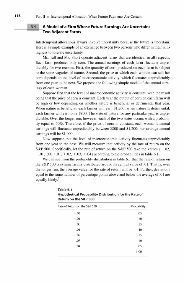
6.4 A Model of a Firm Whose Future Earnings Are Uncertain:Two Adjacent Farms

Intertemporal allocations always involve uncertainty because the future is uncertain.Here is a simple example of an exchange between two persons who differ in their will-ingness to tolerate uncertainty.

Ms. Tall and Ms. Short operate adjacent farms that are identical in all respects.Each farm produces only corn. The annual earnings of each farm fluctuate unpre-dictably for two reasons. First, the quantity of corn produced on each farm is subjectto the same vagaries of nature. Second, the price at which each woman can sell hercorn depends on the level of macroeconomic activity, which fluctuates unpredictablyfrom one year to the next. We propose the following simple model of the annual earn-ings of each woman.

Suppose first that the level of macroeconomic activity is constant, with the resultbeing that the price of corn is constant. Each year the output of corn on each farm willbe high or low depending on whether nature is beneficial or detrimental that year.When nature is beneficial, each farmer will earn $1,200; when nature is detrimental,each farmer will earn only $800. The state of nature for any particular year is unpre-dictable. Over the longer run, however, each of the two states occurs with a probabil-ity equal to 50%. Therefore, if the price of corn is constant, each woman’s annualearnings will fluctuate unpredictably between $800 and $1,200; her average annualearnings will be $1,000.

Now suppose that the level of macroeconomic activity fluctuates unpredictablyfrom one year to the next. We will measure that activity by the rate of return on theS&P 500. Specifically, let the rate of return on the S&P 500 take the values {�.02,�.01, .00, �.01, �.02, �.03, �.04} according to the probabilities in table 6.1.

We can see from the probability distribution in table 6.1 that the rate of return onthe S&P 500 is symmetrically distributed around its central value of .01. That is, overthe longer run, the average value for the rate of return will be .01. Further, deviationsequal to the same number of percentage points above and below the average of .01 areequally likely.7


Table 6.1Hypothetical Probability Distribution for the Rate ofReturn on the S&P 500

Rate of Return on the S&P 500 Probability

�.02 .05

�.01 .10

.00 .15

.01 .40

.02 .15

.03 .10

.04 .05

1.00

Assume that the price of corn is positively correlated with the rate of return on theS&P 500. When the level of economic activity is high, consumers increase their will-ingness to pay high prices for fresh vegetables, with the result that the price of corn ishigh. Similarly, when economic activity is low, the price of corn is low; consumersbegin to economize, with the result that they are less willing to pay for fresh corn.

The earnings of Ms. Short and Ms.Tall will vary positively with both the level ofeconomic activity (through its effect on the price of corn) and with the state of nature.We model this joint dependence as follows. Let the earnings on each farm in a givenyear t be determined by the following equation:

Et�$1,000�$200�2($100)[100(St�.01)], (6.3)

in which Et is the level of earnings on one farm for the year t, St is the rate of return onthe S&P 500 for year t, and 2 is the constant that measures the sensitivity of the farm’searnings for year t to the level of macroeconomic activity in that year.

Equation (6.3) states that the earnings on a farm for year t will be equal to $1,000,plus an adjustment to allow for the effect of nature in that year, plus a further adjust-ment to allow for the effect of the level of macroeconomic activity that year. Theadjustment for the effect of nature is �$200 or �$200, depending on whether or notnature has a beneficial or a detrimental effect on the production of corn that year.

The adjustment for the level of macroeconomic activity is determined by theamount by which the rate of return on the S&P 500 deviates in year t from its average,and by the sensitivity of the farm’s earnings to variations in the level of macroeco-nomic activity. The deviation of the rate of return on the S&P 500 from its averagefluctuates unpredictably from year to year according to the probabilities specified intable 6.1. The term (St�.01) is the deviation in year t of the rate of return on the S&P500 from its average value of .01 The term 100 inside the square brackets converts thisdeviation to the equivalent number of percentage points. The sensitivity of the farm’searnings to fluctuations in macroeconomic activity is measured by the constant 2. Onaverage, every variation of one percentage point in the rate of return on the S&P 500leads to a change in the level of the farm’s earnings equal to (2)($100), or $200. Theterm $100 converts deviations in the rate of return on the S&P 500 to deviations in thelevel of earnings on the farm.

Note that the average level of annual earnings on the farm is equal to $1,000, becausethe average adjustment for nature and the average adjustment for macroeconomic activityare both equal to zero. Since beneficial and detrimental effects of nature occur with equalfrequency, the adjustments of �$200 and �$200 average to zero. The distribution ofvalues for the rate of return on the S&P 500 are symmetrically distributed around thevalue .01. Consequently, the average value of the term (St �.01) is also equal to zero.

The range over which the annual earnings can fluctuate runs from a low of $200 toa high of $1,800. Earnings for year t will take their minimal value of $200 if in that yearnature is detrimental and the rate of return on the S&P 500 takes its lowest value, whichis �.02. The detrimental effect of nature will depress earnings by $200. A rate of returnon the S&P 500 for year t equal to �.02 is a negative deviation of three percentagepoints from its average value. The low level of macroeconomic activity will depressearnings on the farm by (2)($100)(3), or $600. Then the combined effect in year t ofnature and the macroeconomy will be to depress earnings on the farm by $800.


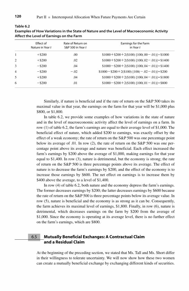
Similarly, if nature is beneficial and if the rate of return on the S&P 500 takes itsmaximal value in that year, the earnings on the farm for that year will be $1,000 plus$800, or $1,800.

In table 6.2, we provide some examples of how variations in the state of natureand in the level of macroeconomic activity affect the level of earnings on a farm. Inrow (1) of table 6.2, the farm’s earnings are equal to their average level of $1,000. Thebeneficial effect of nature, which added $200 to earnings, was exactly offset by theeffect of a weak economy; the rate of return on the S&P 500 was one percentage pointbelow its average of .01. In row (2), the rate of return on the S&P 500 was one per-centage point above its average and nature was beneficial. Each effect increased thefarm’s earnings by $200 above the average of $1,000, making earnings for that yearequal to $1,400. In row (3), nature is detrimental, but the economy is strong; the rateof return on the S&P 500 is three percentage points above its average. The effect ofnature is to decrease the farm’s earnings by $200, and the effect of the economy is toincrease those earnings by $600. The net effect on earnings is to increase them by$400 above the average, to a level of $1,400.

In row (4) of table 6.2, both nature and the economy depress the farm’s earnings.The former decreases earnings by $200; the latter decreases earnings by $600 becausethe rate of return on the S&P 500 is three percentage points below its average value. Inrow (5), nature is beneficial and the economy is as strong as it can be. Consequently,the farm achieves its maximal level of earnings, $1,800. Finally, in row (6), nature isdetrimental, which decreases earnings on the farm by $200 from the average of$1,000. Since the economy is operating at its average level, there is no further effecton the farm’s earnings, which are $800.

6.5 Mutually Beneficial Exchanges: A Contractual Claimand a Residual Claim

At the beginning of the preceding section, we stated that Ms. Tall and Ms. Short differin their willingness to tolerate uncertainty. We will now show how these two womencan create a mutually beneficial exchange by exchanging different kinds of securities.


Table 6.2Examples of How Variations in the State of Nature and the Level of Macroeconomic ActivityAffect the Level of Earnings on the Farm

Effect of Rate of Return on Earnings for the FarmNature in Year t S&P 500 in Year t in Year t

1 �$200 .00 $1000�$200�2($100) [100(.00�.01)]�$1000

2 �$200 .02 $1000�$200�2($100) [100(.02�.01)]�$1400

3 �$200 .04 $1000�$200�2($100) [100(.04�.01)]�$1400

4 �$200 �.02 $1000�$200�2($100) [100(�.02�.01)]�$200

5 �$200 .04 $1000�$200�2($100) [100(.04�.01)]�$1800

6 �$200 .01 $1000�$200�2($100) [100(.01�.01)]�$800

One security is a contractual claim. Its owner agrees to a reduction in the averagereturn that she could have had in exchange for being insulated against the unpre-dictable fluctuations in her rate of return from one year to the next. The other securityis a residual claim. Its owner insulates the holder of the contractual claim against risk.In exchange, the holder of the residual claim receives both a higher average rate ofreturn and a higher volatility of that rate of return. In a more general model, investorscould trade levels of risk by exchanging securities issued by firms that have differentsensitivities to fluctuations in the level of macroeconomic activity.

Consider the two adjacent farms that we described in section 6.4. Ms. Tall ownsone farm; Ms. Short owns the other. The annual earnings on each farm fluctuateunpredictably between a low of $200 and a high of $1,800. The average annualearnings on each farm are $1,000.

Ms. Tall is highly risk averse; specifically, she would prefer to have a guaranteedannual income of $600, rather than an annual income that has an average of $1,000.

Ms. Short is less risk averse than her neighbor. If she can have the total of theincomes from both farms each year, then she will guarantee an annual income of $600to Ms. Tall. Under this arrangement, Ms. Short’s average annual income will be equalto $1,400, which is a gain of $400 over what her average income would be if shedepended only on her own farm and did not provide a guaranteed annual income toMs. Tall. Here is the reason: the income on each farm varies over the interval from$200 to $1,800. Therefore, the sum of the incomes from the two farms will vary overthe interval from $400 to $3,600. Since both the firm-specific variations and the sys-tematic variations are symmetric, the average of the sum of the annual incomes will be($400�$3,600)/2, or $2,000. Allowing for the $600 that Ms. Short will pay to Ms.Talleach year, Ms. Short’s average annual income will be $1,400.

In gaining an increase of $400 in her average annual income, Ms. Short mustaccept an increase in the range over which her income will vary. If she depends onlyon her own farm and makes no guarantee to Ms.Tall, Ms. Short’s income will varyover the range from $200 to $1,800. When Ms. Short enters the new arrangement, herincome will vary over the interval from �$200 to $3,000. Note that the average overthis range is (�$200�$3,000)/2�$2,800/2�$1,400.

The lowest value for Ms. Short’s income will be �$200. This will occur if theincome on each farm takes its lowest value, which is $200. In that event, the sum ofthe farms’ incomes will be $400, and Ms. Short will have to borrow (either from abank or from herself) $200 to make the guaranteed payment of $600 to Ms. Tall. Themaximal value that Ms. Short’s income can take is $3,000. This will occur if eachfarm produces its maximal income, which is $1,800. In that event, the sum of thefarms’ incomes will be $3,600. After paying the guaranteed $600 to Ms. Tall, Ms.Short will have an income of $3,000.

The two women have made a mutually beneficial exchange. The highly risk-averse Ms. Tall trades away $400 of her average annual income of $1,000 in exchangefor a guarantee against unpredictable fluctuations in her income. The less risk-averseMs. Short accepts an increase in the range over which her income will fluctuate, inexchange for an increase of $400 in her average income.

Ms. Tall holds a contractual claim; she will receive $600 each year regardless ofboth the state of nature and the level of macroeconomic activity. Ms. Short will absorb


the vagaries of both nature and the macroeconomy by holding a residual claim; eachyear she will receive whatever is left over from the aggregate income of the two farmsafter Ms. Tall is paid her contractual $600.

Ms. Tall and Ms. Short have created a mutually beneficial exchange that involvesthe levels of their average incomes and ranges over which their annual incomes vary.Financial markets facilitate these exchanges by enabling firms to offer different kindsof securities. The contractual claim that Ms. Tall holds is analogous to a bond; theresidual claim that Ms. Short holds is analogous to a common stock.

6.6 The Equilibrium Prices of the Bond and the Stock

6.6.1 Equilibrium Values for Prices and Rates of Return

We know from the preceding chapters that when future payments are certain, there isan equilibrium relationship between the sequence of payments generated by a secu-rity, the price of that security, and the rate of return that an investor can earn by hold-ing that security. This equilibrium relationship is determined through the applicationof opportunity costs. Specifically, given the level of earnings generated by the secu-rity, the price of the security must be such that the rate of return investors can earn byholding the security will just offset the opportunity cost they incur by not placing theirmoney in a bank.

The equilibrium price of a security is the present value of the sequence of futurepayments associated with that security, using the bank’s rate of interest to discount thefuture payments. If the interest (or discount) rate changes, the price of the security willchange in a way to maintain equality between the opportunity costs of holding thesecurity or holding a bank account of equal value. That is, corresponding to a bank’sinterest rate (which is determined mainly by macroeconomic conditions), there is anequilibrium value for the price of the security.

There is an analogous relationship when future payments are uncertain. There isan equilibrium relationship between the price of a security and the risk-adjusted dis-count rate for the future payments generated by that security. The value for the risk-adjusted discount rate is determined by the market price of risk and by the quantity ofrisk contained in that security.

In the next two subsections, we derive the equilibrium price and discount rates forthe bond held by Ms. Tall and for the stock held by Ms. Short.

6.6.2 The Equilibrium Price of the Bond

The bond is a contractual claim on the income generated by the firm formed by com-bining the two farms. The holder of the bond, Ms. Tall, is entitled to receive $600 peryear regardless of instances of firm-specific risk or systematic risk. We shall supposethat all investors regard the bond as riskless. That is, investors believe that Ms. Shortwill always pay the guaranteed $600 per year, even if in a given year she must borrow (either from a bank or from herself) to do so. This assumption is tantamount toassuming that investors believe that Ms. Short will use her high average earnings to


accumulate a balance in the bank that is sufficient to honor the guarantee in those(relatively infrequent) years when the earnings of the firm are less than $600.Remember, the earnings will be never be less than $400, and that will occur only ifduring the same year the conditions for growing corn are poor and the level of macro-economic activity takes its minimal value.

If investors regard the bond as riskless, then the appropriate discount rate is thebank’s interest rate. If this rate is .10, then the equilibrium price of the bond is:

PB�($600 per year)/(.10 per year)�$6,000. (6.4)

6.6.3 The Equilibrium Price of the Stock

The stock is a residual claim on the firm’s earnings. Ms. Short, who holds the stock, isentitled each year to whatever remains of the firm’s earnings after Ms. Tall is paid$600. As we established in section 6.4, Ms. Short’s average annual income is $1,400.Her income in any year will fluctuate due not only to the vagaries of nature but also tothe unpredictable fluctuations in the level of macroeconomic activity. The vagaries ofnature contribute firm-specific risk to Ms. Short’s annual income. But firm-specificrisk is diversifiable, and thus not rewardable. We can ignore it in determining the rateof return that Ms. Short can expect to earn by holding the stock.

The sensitivity of the rate of return on Ms. Short’s stock to the unpredictable fluc-tuations in the level of macroeconomic activity is the systematic risk for that stock.Ms. Short cannot eliminate this risk by holding her stock as part of a diversified port-folio.8 Therefore, the quantity of systematic risk associated with her stock will affectits equilibrium rate of return.

The contribution of the systematic risk associated with Ms. Short’s stock to theequilibrium rate of return on that stock is determined by the sensitivity of the firm’searnings to variations in the level of macroeconomic activity. In our example, the levelof this sensitivity is 2. Since the market price of risk is .04, the equilibrium risk-adjusted rate of return on the stock is the reward for waiting plus the reward for bear-ing risk, or:

In equilibrium, Ms. Short should receive an average rate of return equal to 18%,which consists of 10% as a reward for waiting and 8% as a reward for bearing risk. IfMs. Short is to receive an average rate of return equal to 18%, then the price of thestock must be the present value of her average earnings from the stock, discounted atthe rate of 18%. Since her average annual earnings will be equal to $1,400, we con-clude that the equilibrium price of the stock is:

Equilibrium price of the stock [$1400 per year]/[.18 per year]

$7,

�

� 7777.78.

Equilibrium rate of return on the stock

Reward for

risk-adjusted

� wwaiting Reward for bearing risk

Reward for waiting (market pric

�

� � ee of risk) (quantity of risk)

.10 [.04][2] .10 .08 .18.� � � � �


(6.5)

(6.6)

Note that the equilibrium price of the stock is less than $14,000, which is theresult we would obtain if we were to capitalize the average earnings of $1,400 peryear by the bank’s interest rate of .10 per year. Ms. Short’s average annual earningsfrom her stock are $1,400. Since her earnings are sensitive to changes in the level ofmacroeconomic activity, and thus fluctuate unpredictably around this average, it isinappropriate to discount the average of these risky earnings by using the risk-free dis-count rate. The appropriate discount rate to calculate the price of the stock is deter-mined by the sensitivity of the earnings on the stock to changes in the level ofmacroeconomic activity. Ms. Short is compensated for bearing risk (and thereby insu-lating Ms. Tall from risk) by being able to purchase the right to receive an average of$1,400 per year by paying less than $14,000. Using the concept of opportunity costs,it is easy to show that competition among investors seeking a risk-free profit willensure that the price of a right to receive a guaranteed annual income of $1,400 will be$14,000, when banks pay interest at the rate of .10 per year.

Suppose that the price of a security that pays a guaranteed $1,400 per year were$13,500. An investor could purchase the security using $13,500 borrowed from abank. One year later, the investor would realize a profit equal to $50 because he wouldreceive $1,400 from the security and owe only $1,350 in interest to the bank; (.10)($13,500)�$1,350. If the bank were willing to leave the principal of the loan out-standing and collect only the interest each year, the investor would realize a profit of$50 per year. If the bank insisted on having the loan paid off at the end of one year, theinvestor could do so by selling the security for $13,500. Whether or not the investorpays off the loan at the end of the first year, he still realizes a profit of $50 for thatyear. Competition among investors seeking this profit will force the price of the secu-rity up to $14,000. At this price, investors cannot obtain a profit by purchasing thesecurity using funds borrowed from a bank that charges interest at .10 per year.

The reader should replicate the foregoing argument for the case in which the priceof the security is above its equilibrium value of $14,000.

6.7 Conclusion

A financial security is a saleable right to receive a sequence of future payments. In thepreceding chapters, we restricted our attention to cases in which all investors knowwith certainty today what those future payments will be. Under this restriction, weexplained that the current price of a security is the present value of the future pay-ments that will accrue to the investor who holds that security. That present value iscalculated by discounting each future payment by the interest rate that banks will payon deposits.

In the present chapter, we have shown that the principles that govern the pricingof financial securities when there is no uncertainty about future payments have analo-gous applications when future payments are uncertain. To allow for uncertainty, weuse a risk-adjusted discount rate. Under modern portfolio theory, the adjustment forrisk depends only on the sensitivity of the rate of return on that security to the level ofmacroeconomic activity. The justification for this is that rational investors can avoid


firm-specific risk by holding well-diversified portfolios. But investors cannot escapethe effects on a security’s rate of return of the unpredictable volatility in the level ofmacroeconomic activity. This effect is systematic risk. Economists measure the levelof macroeconomic activity by the rate of return on a diversified portfolio such as theS&P 500.

In the preceding chapters, we also examined how financial markets promotemutually beneficial intertemporal exchanges, again assuming that there is no uncer-tainty about future payments. We stated that economic efficiency in the allocation ofscarce resources requires that the financial markets are informationally efficient. Inparticular, managers of firms need to know the rates at which investors are willing tosubstitute between present and future consumption. Similarly, investors need accurateinformation about the rates at which proposed investment projects will generate futureearnings. These observations apply also to an economy in which there is uncertaintyabout future earnings. To examine how, and how well, financial markets allocateresources under uncertainty, we need to develop models of how the markets set theprices of securities when future earnings are uncertain.

How could managers determine the rates at which an investor is willing to substi-tute between present and future consumption, and between the average rate of returnon a project and the volatility of that rate of return? How should managers chooseinvestment projects and methods of financing them if investors have different rates atwhich they are willing to substitute between the present and the future, and betweenaverage return and volatility?

The answers are analogous to questions we raised (and answered) in chapter 4. Inthat chapter, we concluded that in equilibrium every investor would allocate herwealth between present and future consumption so that the marginal value of presentconsumption is equal to 1�r (where r is the rate of interest). That is, in equilibrium,the marginal value of one more dollar of present consumption is equal to an additional(1�r) dollars in future consumption. Since every investor faces the same value for theinterest rate, r, all investors place the same marginal value on present consumption.Therefore, managers should undertake all projects whose rates of return exceed theinterest rate.

When future payments are uncertain, managers should use risk-adjusted interestrates to determine which projects to undertake. We explain how to obtain these risk-adjusted interest rates in part IV, where we derive modern portfolio theory.

In part III, we present those elements of probability and statistics that we use inpart IV to derive modern portfolio theory and its empirical implications for the pricesof financial securities. Then in part V, we use these tools to address specific questionsabout the efficacy of financial markets in promoting economic efficiency.

Problems

1. Suppose that the interest rate on a government bond is .10, and that the marketprice of risk is equal to .05. In addition, suppose that, on average, the change in therate of return on Security K from one year to the next is equal to 2.5 times the changein the rate of return on the S&P 500 over the same period.


(a) What is the reward for waiting? What is the quantity of risk in Security K?(b) According to the capital asset pricing model, what is the equilibrium average

rate of return on Security K?(c) How much additional risk must an investor accept for each additional one

percentage point of average rate of return? Describe how the investor shouldrestructure his portfolio to gain an additional one percentage point of averagerate of return.

2. Suppose that the price of a security that is guaranteed to pay $2,000 per year is$19,000. Explain how an investor could purchase the security using funds borrowedfrom a bank (at a rate of .10 per year) and make a risk-free profit of $100 per year? Ifthe price of the same security were $21,000, what would the investor do?

Notes

1. In fact, the bond does carry the risk that the government might inflate the general level ofprices by printing too much money relative to the supply of goods and services. In this event,the bondholders would suffer a loss of purchasing power. To address this problem, the govern-ment now offers bonds on which the payments of interest are periodically adjusted for inflation.

2. The names of the Nobel laureates and a selected bibliography of their works appear at theend of the book.

3. A bond whose issuer makes no periodic payments of interest is called a zero coupon bond.Until the early twentieth century, bonds were issued as certificates, the borders of which weredivided into coupons. Each coupon bore a date on which a payment of interest was due. Whenan interest payment came due, the owner of the bond would clip the appropriate coupon andpresent it to the bank that made the payments of interest as an agent of the firm that issued thebond. The coupon rate of a bond was the percentage of the bond’s face value that the issuingfirm was obligated to pay annually as interest. Investors who owned bonds were known ascoupon clippers. Bond certificates no longer have coupons. It is more efficient, and safer, torecord the name of the owner of a bond and make payments electronically than to rely on themailing and storage of physical coupons. The term coupon rate survives, however, as the per-centage of a bond’s face value that is to be paid annually as interest. Hence, a zero coupon bond,or a zero, is a bond on which there are no annual payments of interest. The owner of the bondreceives interest implicitly because the bond is sold initially (by the issuing firm) at a price thatis less than the bond’s face value that the issuer must pay at the maturity date of the bond.

4. The net effect on the investors’ earnings will depend on the relative amounts of money thatthey have invested in the two firms. We explain this in chapter 8.

5. By including securities of both American and foreign firms in their portfolios, investorscan eliminate some of the risk that they would bear if they held only American securities. For aportfolio that is diversified across several countries, the relevant macroeconomic system is theworld economy. The level of systematic risk for a security in this portfolio is the sensitivity ofthe rate of return on that security to unpredictable fluctuations in the rate of return for the worldeconomy. The calculation of this rate of return is problematic; we do not pursue this matterfurther.

6. The asset pricing models in modern portfolio theory hold that the equilibrium price of asecurity does not depend on the amount of firm-specific risk in that security. In some of themore recent (and more complicated) models, the equilibrium price of a security does depend onthe firm-specific risk in that security.


7. Sometimes there is confusion between a percentage and a percentage point. Suppose that abank increases the rate of interest that it pays on deposits from .04 per year to .05 per year. Theincrease in the rate of interest by one percentage point, from .04 to .05, is a 25% increase in therate of interest, since (.05�.04)/.04�.25.

8. Holding the stock as part of a properly diversified portfolio will, however, minimize thefirm-specific risk. We define a properly diversified portfolio in chapter 8.



Part III

Rates of Return as RandomVariables


7.1 The Objectives of Using Probabilistic Models

Financial markets promote mutually beneficial intertemporal exchanges by reducingthe costs for individuals to buy and sell financial securities. The securities are rightsto receive sequences of future payments. The economics of financial markets is a sys-tematic study of how, and how well, these markets promote mutually beneficialexchanges. To answer these questions, economists must first explain the principlesthat govern how financial markets set the prices of securities.

In the preceding chapters, we analyzed a simple version of this question byassuming that there is no uncertainty about either the timing or the size of any futurepayment. Using this assumption, we could easily develop the concepts of presentvalue and opportunity cost. These concepts underlie the central principle that governsthe prices of financial securities. This principle is that competition among investorsand firms causes the relative prices of securities to adjust so that investors have noincentive to reallocate their funds among securities, and firms have no incentive tochange their decisions on which securities to issue and which projects to undertake. Ifthe relative prices of securities have adjusted so as to produce these effects, the mar-ket has produced an equilibrium configuration of prices. In this equilibrium, the priceof each security is the present value of its associated sequence of future payments, andthis present value is equal to all the costs, including the opportunity costs, that aninvestor must incur to purchase the right to receive that sequence of payments.

In reality, of course, future payments are not certain. Some borrowers renege ontheir promises to pay. The unpredictable variations in firms’ future earnings creates agreater problem. A firm relies on its future earnings to pay interest and dividends onits securities. Few firms can predict their earnings with certainty. A firm’s earningswill be affected by variations in the demand for its products and in the costs of itsinputs. In particular, variations in interest rates will affect a firm’s earnings by chang-ing the costs of carrying inventories.1

The price of a financial security takes into account any unpredictable variation infuture payments. Economists do this by using the concept of a random variable. A ran-dom variable is a variable that takes values according to a probabilistic process. Aprobabilistic process is a process that generates values according to the unpredictableoutcomes of an experiment. For example, define the random variable Y as the totalnumber of red cards that one will obtain after drawing one card from each of two

7 Probabilistic Models

131

decks. The possible values for Y are 0, 1, and 2. Suppose that it is equally likely todraw either a red card or a black card from a given deck. Further, suppose that the twodraws are independent in the sense that the outcome of the draw from one deck hasno effect on the outcome of the draw from the other deck. Under these conditions, Ywill take the value 0 with probability 0.25, the value 1 with probability 0.5, and thevalue 2 with probability 0.25.2

In chapters 1 through 5, we conducted our analyses in terms of the prices of finan-cial securities rather than in terms of their rates of return. This was convenientbecause, under the assumption that there is no uncertainty about future payments,there is, in equilibrium, only one rate of return. This is the rate of interest paid bybanks. In equilibrium, the difference between the prices of any two securities willcompensate investors for the differences in the timing and the sizes of the paymentsgenerated by the two securities. Competition among investors will adjust the price ofeach security so that investors who receive the sequence of payments generated bythat security will receive a rate of return equal to the rate of interest that they couldreceive by depositing their money in a bank.

In chapter 6, we considered a simple model in which future payments are uncer-tain. In that case, investors will create mutually beneficial exchanges based on theirdifferences in willingness to bear risk. In equilibrium, competition among investorswill adjust the prices of securities so that their average rates of return will compensateinvestors for the levels of risk in those securities. Since securities differ in their levelsof risk, they will differ in their average rates of return. We saw an example of this inchapter 6 in the difference between the average rate of return on the bond held by Ms. Tall and the average rate of return on the stock held by Ms. Short.

For much of the analysis in the remainder of this book, it will be more conven-ient to focus on the probability distribution of the rates of return on a security, ratherthan on its price. We define equilibrium in a financial market as a set of alternativecombinations of risk and average rate of return that are available to investors.Competition among investors will adjust the probability distribution of the rate ofreturn on each security so that each security offers one of the equilibrium combina-tions of average rate of return and risk.

To understand the concept of equilibrium as a set of alternate combinations ofrisk and average rate of return, we represent the rate of return on a security as a ran-dom variable, and develop properties of the probability distribution of that randomvariable.

7.2 Rates of Return and Prices

In this section, we explain the relationship between the rate of return on a security andthe price of that security. Assume that securities can be bought or sold only at discretetimes. Let t designate any one of these times, and let t take the values t�0, t�1, t�2,and so on. The present moment is t�0. Payments of dividends or interest occur onlyat these times. An investor who purchases a security at time t will not receive any div-idend or interest that is paid on that security at time t. He will not be eligible to receive

Part III ■ Rates of Return as Random Variables132

dividends or interest on that security until time t�1. The investor who sells the secu-rity at time t receives whatever interest or dividend is paid at that time. We say thatsecurities are sold ex dividend, or ex interest.3

The rate of return on a security over one period of time is the change in its priceover that period plus the dividend or interest paid during or at the end of that period.For convenience, we consider only stocks, so that the only payment that can occur isa dividend.

Let ri,t be the rate of return on Security i from time t�1 to time t. Let Pi,t�1 be itsprice at time t�1, and Pi,t be its price at time t. Finally, let Di,t be the dividend paid(per share) during the period that ends at time t. If the firm pays no dividend duringthat period, then Di,t will be zero.4

The rate of return ri,t is defined by:

(7.1)

The variable ri,t is the rate at which an investment in Security i will change in valuefrom time t�1 to time t, with the rate of change measured per dollar invested inSecurity i at time t�1. The difference in prices, Pi,t�Pi,t�1, is the capital gain or loss,and Di,t is the dividend. Clearly, the rate of return can be negative if the price fallsfrom time t�1 to time t by an amount that exceeds the size of the dividend.

The definition of the rate of return ri,t does not require that the investor purchasedSecurity i at time t�1; she could have purchased it earlier. Nor does the definitionrequire that she sell Security i at time t. Consistent with the concept of opportunitycosts, the definition of rate of return in equation (7.1) recognizes that an investor whopurchased Security i prior to time t�1 had the opportunity to sell it at that time forPi,t�1 in cash. A decision at time t�1 to continue to hold a share of Security i that theinvestor bought at an earlier time is economically equivalent to a decision to purchasea share of Security i at time t�1.5 Either decision is a decision to hold wealth fromtime t�1 to time t in the form of a share of Security i rather than in the form of a quan-tity of cash equal to Pi,t�1. To decide not to sell at time t�1 a share acquired previ-ously is an implicit decision to forego holding Pi,t�1 in cash. To decide to purchase ashare at time t�1 is an explicit decision to forego holding the cash.

The same logic applies at time t. The critical point is to distinguish between thelevel of the investor’s wealth and the form in which the investor holds that wealth.

Consider at time t two investors, Mr. Croton and Ms. Harmon. Mr. Croton ownsone share of Security i, and Ms. Harmon owns an amount of cash equal to Pi,t. Bothinvestors hold the same level of wealth at time t; they differ only in the forms in whichthey hold their wealth. The share of stock and the quantity of money are interchange-able. At time t, a decision by Mr. Croton to continue holding his wealth in the form ofone share of Security i is economically equivalent to a decision by Ms. Harmon topurchase one share of Security i. Again, we see an instance of opportunity cost andthe distinction between implicit and explicit expenditures. By choosing not to sell hisone share of Security i, Mr. Croton has implicitly chosen to forego the opportunity toincrease his holdings of cash by the amount Pi,t. Analogously, by purchasing one shareof Security i at the price Pi,t, Ms. Harmon has explicitly chosen to decrease her hold-ings of cash by that amount.6

rP P D

Pi ti t i t i t

i t,

, , 1 ,

, 1

( ).�

� ��

�

Chapter 7 ■ Probabilistic Models 133

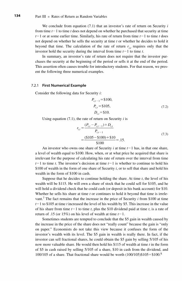
We conclude from equation (7.1) that an investor’s rate of return on Security ifrom time t�1 to time t does not depend on whether he purchased that security at timet�1 or at some earlier time. Similarly, his rate of return from time t�1 to time t doesnot depend on whether he sells the security at time t or whether he decides to hold itbeyond that time. The calculation of the rate of return ri,t requires only that theinvestor hold the security during the interval from time t�1 to time t.

In summary, an investor’s rate of return does not require that the investor pur-chases the security at the beginning of the period or sells it at the end of the period.This assertion often causes trouble for introductory students. For that reason, we pres-ent the following three numerical examples.

7.2.1 First Numerical Example

Consider the following data for Security i:

(7.2)

Using equation (7.1), the rate of return on Security i is

(7.3)

An investor who owns one share of Security i at time t�1 has, in that one share,a level of wealth equal to $100. How, when, or at what price he acquired that share isirrelevant for the purpose of calculating his rate of return over the interval from timet�1 to time t. The investor’s decision at time t�1 is whether to continue to hold his$100 of wealth in the form of one share of Security i, or to sell that share and hold hiswealth in the form of $100 in cash.

Suppose that he decides to continue holding the share. At time t, the level of hiswealth will be $115. He will own a share of stock that he could sell for $105, and hewill hold a dividend check that he could cash (or deposit in his bank account) for $10.Whether he sells his share at time t or continues to hold it beyond that time is irrele-vant.7 The fact remains that the increase in the price of Security i from $100 at timet�1 to $105 at time t increased the level of his wealth by $5. This increase in the valueof his share from time t�1 to time t, plus the $10 dividend paid at time t, is a rate ofreturn of .15 (or 15%) on his level of wealth at time t�1.

Sometimes students are tempted to conclude that the $5 gain in wealth caused bythe increase in the price of the share does not “really count” because the gain is “onlyon paper.” Economists do not take this view because it confuses the form of theinvestor’s wealth with its level. The $5 gain in wealth is really there. In fact, if theinvestor can sell fractional shares, he could obtain the $5 gain by selling 5/105 of hisnow more valuable share. He would then hold his $115 of wealth at time t in the formof $5 in cash raised by selling 5/105 of a share, $10 in cash from the dividend, and100/105 of a share. That fractional share would be worth (100/105)$105�$100.8

rP P D

Pi ti t i t i t

i t,

, , 1 ,

, 1

( )

($105 $100) $10

$100.15.

��

��

�

�

�

P

P

D

i t

i t

i t

, 1

,

,

$100,

$105,

$10.

� �

�

�


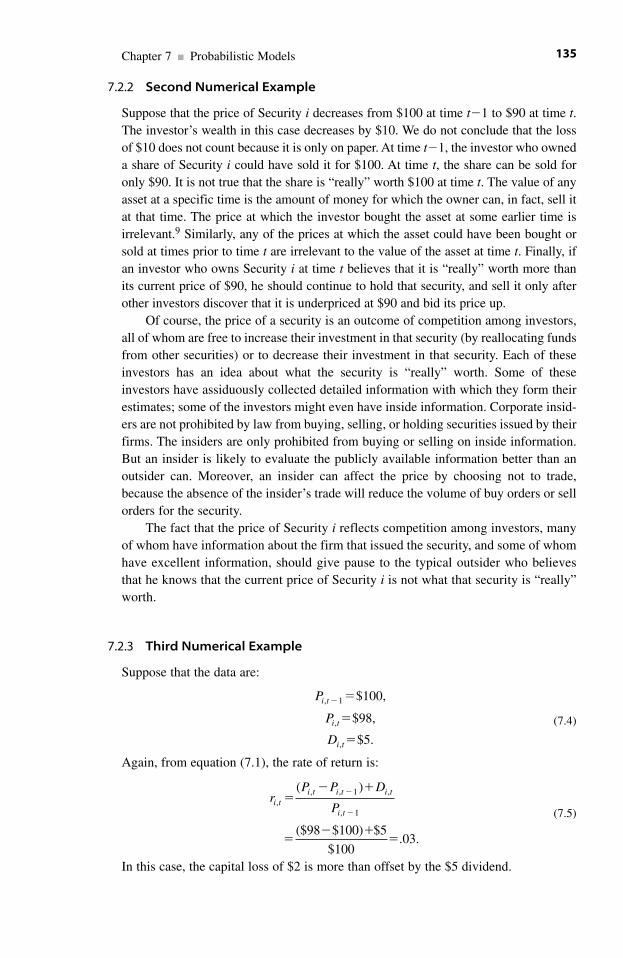
7.2.2 Second Numerical Example

Suppose that the price of Security i decreases from $100 at time t�1 to $90 at time t.The investor’s wealth in this case decreases by $10. We do not conclude that the lossof $10 does not count because it is only on paper. At time t�1, the investor who owneda share of Security i could have sold it for $100. At time t, the share can be sold foronly $90. It is not true that the share is “really” worth $100 at time t. The value of anyasset at a specific time is the amount of money for which the owner can, in fact, sell itat that time. The price at which the investor bought the asset at some earlier time isirrelevant.9 Similarly, any of the prices at which the asset could have been bought orsold at times prior to time t are irrelevant to the value of the asset at time t. Finally, ifan investor who owns Security i at time t believes that it is “really” worth more thanits current price of $90, he should continue to hold that security, and sell it only afterother investors discover that it is underpriced at $90 and bid its price up.

Of course, the price of a security is an outcome of competition among investors,all of whom are free to increase their investment in that security (by reallocating fundsfrom other securities) or to decrease their investment in that security. Each of theseinvestors has an idea about what the security is “really” worth. Some of theseinvestors have assiduously collected detailed information with which they form theirestimates; some of the investors might even have inside information. Corporate insid-ers are not prohibited by law from buying, selling, or holding securities issued by theirfirms. The insiders are only prohibited from buying or selling on inside information.But an insider is likely to evaluate the publicly available information better than anoutsider can. Moreover, an insider can affect the price by choosing not to trade,because the absence of the insider’s trade will reduce the volume of buy orders or sellorders for the security.

The fact that the price of Security i reflects competition among investors, manyof whom have information about the firm that issued the security, and some of whomhave excellent information, should give pause to the typical outsider who believesthat he knows that the current price of Security i is not what that security is “really”worth.

7.2.3 Third Numerical Example

Suppose that the data are:

(7.4)

Again, from equation (7.1), the rate of return is:

(7.5)

In this case, the capital loss of $2 is more than offset by the $5 dividend.

rP P D

Pi ti t i t i t

i t,

, , 1 ,

, 1

( )

($98 $100) $5

$100.03.

��

��

�

�

�

P

P

D

i t

i t

i t

, 1

,

,

$100,

$98,

$5.

� �

�

�


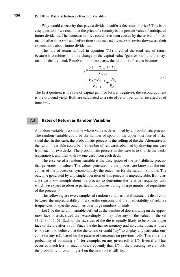
Why would a security that pays a dividend suffer a decrease in price? This is aneasy question if we recall that the price of a security is the present value of anticipatedfuture dividends. The decrease in price could have been caused by the arrival of infor-mation after time t�1 and before time t that caused investors to revise downward theirexpectations about future dividends.

The rate of return defined in equation (7.1) is called the total rate of returnbecause it combines both the change in the capital value (gain or loss) and the pay-ment of the dividend. Resolved into these parts, the total rate of return becomes:

(7.6)

The first quotient is the rate of capital gain (or loss, if negative); the second quotientis the dividend yield. Both are calculated as a rate of return per dollar invested as oftime t�1.

7.3 Rates of Return as Random Variables

A random variable is a variable whose value is determined by a probabilistic process.The random variable could be the number of spots on the uppermost face of a six-sided die. In this case, the probabilistic process is the rolling of the die. Alternatively,the random variable could be the number of red cards obtained by drawing one cardfrom each of two decks. The probabilistic process in this case is to shuffle the decks(separately), and then to draw one card from each deck.

The essence of a random variable is the description of the probabilistic processthat generates its values. The values generated by the process are known as the out-comes of the process or, synonomously, the outcomes for the random variable. Theoutcome generated by any single operation of this process is unpredictable. But (usu-ally) we know enough about the process to determine the relative frequency withwhich we expect to observe particular outcomes during a large number of repetitionsof the process.10

The following are two examples of random variables that illustrate the distinctionbetween the unpredictability of a specific outcome and the predictability of relativefrequencies of specific outcomes over large numbers of trials.

Let Y be the random variable defined as the number of dots showing on the upper-most face of a six-sided die. Accordingly, Y may take any of the values in the set {1, 2, 3, 4, 5, 6}. Each of the six sides of the die is equally likely to be on the upperface of the die after a roll. Since the die has no memory and no consciousness, thereis no reason to believe that the die would or could “try” to display any particular out-come on any roll, based on the pattern of outcomes on previous rolls. Therefore, theprobability of obtaining a 4, for example, on any given roll is 1/6. Even if a 4 hasoccurred much less, or much more, frequently than 1/6 of the preceding several rolls,the probability of obtaining a 4 on the next roll is still 1/6.

rP P D

P

P P

P

D

P

i ti t i t i t

i t

i t i t

i t

i,t

i t

,, , 1 ,

, 1

, , 1

, 1 , 1

( )�

� �

��

�

�

�

�

� �

..


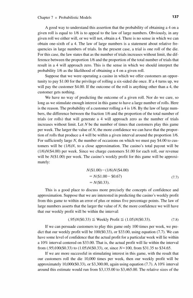
A good way to understand this assertion that the probability of obtaining a 4 on agiven roll is equal to 1/6 is to appeal to the law of large numbers. Obviously, in anygiven roll we either will, or we will not, obtain a 4. There is no sense in which we canobtain one-sixth of a 4. The law of large numbers is a statement about relative fre-quencies in large numbers of trials. In the present case, a trial is one roll of the die.For this case, the law states that as the number of trials increases without limit, the dif-ference between the proportion 1/6 and the proportion of the total number of trials thatresult in a 4 will approach zero. This is the sense in which we should interpret theprobability 1/6 as the likelihood of obtaining a 4 on a given roll.

Suppose that we were operating a casino in which we offer customers an oppor-tunity to pay $1.00 for the privilege of rolling a six-sided die once. If a 4 turns up, wewill pay the customer $4.00. If the outcome of the roll is anything other than a 4, thecustomer gets nothing.

We have no way of predicting the outcome of a given roll. Nor do we care, solong as we stimulate enough interest in this game to have a large number of rolls. Hereis the reason. The probability of a customer rolling a 4 is 1/6. By the law of large num-bers, the difference between the fraction 1/6 and the proportion of the total number oftrials (or rolls) that will generate a 4 will approach zero as the number of trialsincreases without limit. Let N be the number of times that customers play this gameper week. The larger the value of N, the more confidence we can have that the propor-tion of rolls that produce a 4 will be within a given interval around the proportion 1/6.For sufficiently large N, the number of occasions on which we must pay $4.00 to cus-tomers will be (1/6)N, to a close approximation. The casino’s total payout will be(1/6)N($4.00) per week. Since we charge customers $1.00 for each roll, our revenuewill be N($1.00) per week. The casino’s weekly profit for this game will be approxi-mately:

(7.7)

This is a good place to discuss more precisely the concepts of confidence andapproximation. Suppose that we are interested in predicting the casino’s weekly profitfrom this game to within an error of plus or minus five percentage points. The law oflarge numbers asserts that the larger the value of N, the more confidence we will havethat our weekly profit will be within the interval:

(.95)N($0.33) � Weekly Profit � (1.05)N($0.33). (7.8)

If we can persuade customers to play this game only 100 times per week, we pre-dict that our weekly profit will be 100($0.33), or $33.00, using equation (7.7). We canhave some level of confidence that the actual profit for a particular week will lie withina 10% interval centered on $33.00. That is, the actual profit will lie within the intervalfrom (.95)100($0.33) to (1.05)N($0.33), or, since N�100, from $31.35 to $34.65.

If we are more successful in stimulating interest in this game, with the result thatour customers roll the die 10,000 times per week, then our weekly profit will beapproximately 10,000($0.33), or $3,300.00, again using equation (7.7). A 10% intervalaround this estimate would run from $3,135.00 to $3,465.00. The relative sizes of the

N N

N

N

($1.00) (1/6) ($4.00)

($1.00 $0.67)

($0.33).

�

� �

�


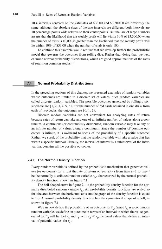
10% intervals centered on the estimates of $33.00 and $3,300.00 are obviously thesame; although the absolute sizes of the two intervals are different, both intervals are10 percentage points wide relative to their center points. But the law of large numbersasserts that the likelihood that the weekly profit will lie within 10% of $3,300.00 whenthe number of trials is 10,000 is greater than the likelihood that the weekly profit willlie within 10% of $33.00 when the number of trials is only 100.

To continue this example would require that we develop further the probabilisticmodel that governs the outcomes from rolling dice. Rather than doing that, we nextexamine normal probability distributions, which are good approximations of the ratesof return on common stocks.11

7.4 Normal Probability Distributions

In the preceding sections of this chapter, we presented examples of random variableswhose outcomes are limited to a discrete set of values. Such random variables arecalled discrete random variables. The possible outcomes generated by rolling a six-sided die are {1, 2, 3, 4, 5, 6}. For the number of red cards obtained in one draw fromeach of two decks, the outcomes are {0, 1, 2}.

Discrete random variables are not convenient for analyzing rates of returnbecause rates of return can take any one of an infinite number of values along a con-tinuum. A continuous (or continuously distributed) random variable may take any ofan infinite number of values along a continuum. Since the number of possible out-comes is infinite, it is awkward to speak of the probability of a specific outcome.Rather, we speak of the probability that the random variable will take a value that lieswithin a specific interval. Usually, the interval of interest is a subinterval of the inter-val that contains all the possible outcomes.

7.4.1 The Normal Density Function

Every random variable is defined by the probabilistic mechanism that generates val-ues (or outcomes) for it. Let the rate of return on Security i from time t�1 to time tbe the normally distributed random variable ri,t, characterized by the normal probabil-ity density function, shown in figure 7.1.

The bell-shaped curve in figure 7.1 is the probability density function for the nor-mally distributed random variable ri,t. All probability density functions are scaled sothat the area between the horizontal axis and the graph of the density function is equalto 1.0. A normal probability density function has the symmetrical shape of a bell, asshown in figure 7.1.

We can now define the probability of an outcome for ri,t. Since ri,t is a continuousrandom variable, we define an outcome in terms of an interval in which the value gen-erated for ri,t will lie. Let rA and rB, with rA rB, be fixed values that define an inter-val of potential values for ri,t.


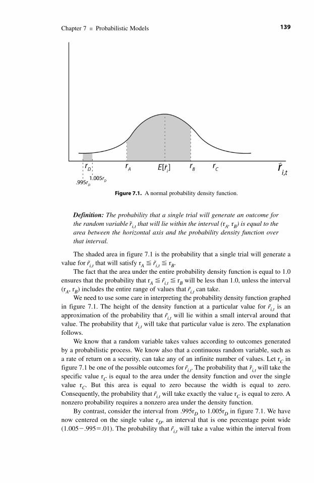
Definition: The probability that a single trial will generate an outcome forthe random variable ri,t that will lie within the interval (rA, rB) is equal to thearea between the horizontal axis and the probability density function overthat interval.

The shaded area in figure 7.1 is the probability that a single trial will generate avalue for ri,t that will satisfy rA � ri,t � rB.

The fact that the area under the entire probability density function is equal to 1.0ensures that the probability that rA � ri,t � rB will be less than 1.0, unless the interval(rA, rB) includes the entire range of values that ri,t can take.

We need to use some care in interpreting the probability density function graphedin figure 7.1. The height of the density function at a particular value for ri,t is anapproximation of the probability that ri,t will lie within a small interval around thatvalue. The probability that ri,t will take that particular value is zero. The explanationfollows.

We know that a random variable takes values according to outcomes generatedby a probabilistic process. We know also that a continuous random variable, such asa rate of return on a security, can take any of an infinite number of values. Let rC infigure 7.1 be one of the possible outcomes for ri,t. The probability that ri,t will take thespecific value rC is equal to the area under the density function and over the singlevalue rC. But this area is equal to zero because the width is equal to zero.Consequently, the probability that ri,t will take exactly the value rC is equal to zero. Anonzero probability requires a nonzero area under the density function.

By contrast, consider the interval from .995rD to 1.005rD in figure 7.1. We havenow centered on the single value rD, an interval that is one percentage point wide(1.005�.995�.01). The probability that ri,t will take a value within the interval from


Figure 7.1. A normal probability density function.

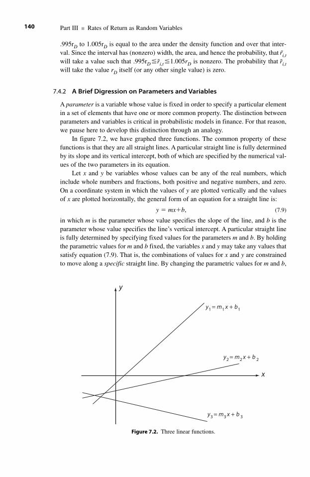
.995rD to 1.005rD is equal to the area under the density function and over that inter-val. Since the interval has (nonzero) width, the area, and hence the probability, that ri,twill take a value such that .995rD �ri,t �1.005rD is nonzero. The probability that ri,twill take the value rD itself (or any other single value) is zero.

7.4.2 A Brief Digression on Parameters and Variables

A parameter is a variable whose value is fixed in order to specify a particular elementin a set of elements that have one or more common property. The distinction betweenparameters and variables is critical in probabilistic models in finance. For that reason,we pause here to develop this distinction through an analogy.

In figure 7.2, we have graphed three functions. The common property of thesefunctions is that they are all straight lines. A particular straight line is fully determinedby its slope and its vertical intercept, both of which are specified by the numerical val-ues of the two parameters in its equation.

Let x and y be variables whose values can be any of the real numbers, whichinclude whole numbers and fractions, both positive and negative numbers, and zero.On a coordinate system in which the values of y are plotted vertically and the valuesof x are plotted horizontally, the general form of an equation for a straight line is:

y � mx�b, (7.9)

in which m is the parameter whose value specifies the slope of the line, and b is theparameter whose value specifies the line’s vertical intercept. A particular straight lineis fully determined by specifying fixed values for the parameters m and b. By holdingthe parametric values for m and b fixed, the variables x and y may take any values thatsatisfy equation (7.9). That is, the combinations of values for x and y are constrainedto move along a specific straight line. By changing the parametric values for m and b,


x

y

y3 = m3 x + b 3

y2 = m2 x + b 2

y1 = m1 x + b1

Figure 7.2. Three linear functions.

we allow the combinations of values for x and y to move along a different straight line.We now apply this distinction between parameters and variables to our considerationof normal probability density functions.

7.4.3 The Expected Value and the Standard Deviation of a Normally Distributed Random Variable

There is an infinite number of distinct normal probability density functions. A partic-ular normal density function is fully specified by the values assigned to its expectedvalue and its standard deviation, which are its only two parameters. The expectedvalue of a random variable is the sum of the values that the variable can take, witheach value weighted by the probability that the variable can take that value. For a nor-mally distributed random variable, the numerical value of its expected value is thecenter point of its symmetric probability density function. The standard deviation ofa random variable is the positive square root of the sum of squared deviations that thevariable can take from its expected value, with each deviation weighted by the prob-ability that it can occur. The numerical value of the standard deviation determines thespread of the density function. In this subsection, we develop some of the propertiesof the expected value and the standard deviation for a normal density function.12 Firstwe explain why these parameters are important.

The probabilities with which a rate of return will take values within various inter-vals are determined by the probability density function for that rate of return. If thereis a change in the values of either of the parameters that define the density function,there will be changes in the probabilities that govern the outcomes for the rate of return.

A fundamental property of modern portfolio theory is that an individual investorcan, within limits, choose the values of the expected value and the standard deviationof the probability density function that governs the rate of return on the portfolio. Aninvestor can do this by altering the allocation of funds among the individual securitiesin the portfolio. By changing the values of the expected value and the standard devi-ation for the rate of return on the portfolio, an investor can change the probabilitiesthat the rate of return will lie within various intervals.

The expected value is a fixed value of the random variable. The expected valueof a normally distributed random variable is the center point of its symmetric densityfunction. In figure 7.1, the expected value is Er.

The second parameter is the standard deviation, the value of which determines thespread, or dispersion, of the density function around its expected value. Unlike theexpected value, the standard deviation is not a specific value of the random variable.The standard deviation is a measure of dispersion that is defined in the same units asthe random variable. If the random variable is a rate of return, which is defined as apercentage, then the standard deviation is measured in terms of percentage points.

By definition, 68% of the area under a normal density function is contained withinan interval that extends from one standard deviation below the expected value to onestandard deviation above the expected value. An interval that extends from two stan-dard deviations below the expected value to two standard deviations above it contains95% of the area under the density function. In figure 7.3, we have drawn some exam-ples of normal probability density functions.


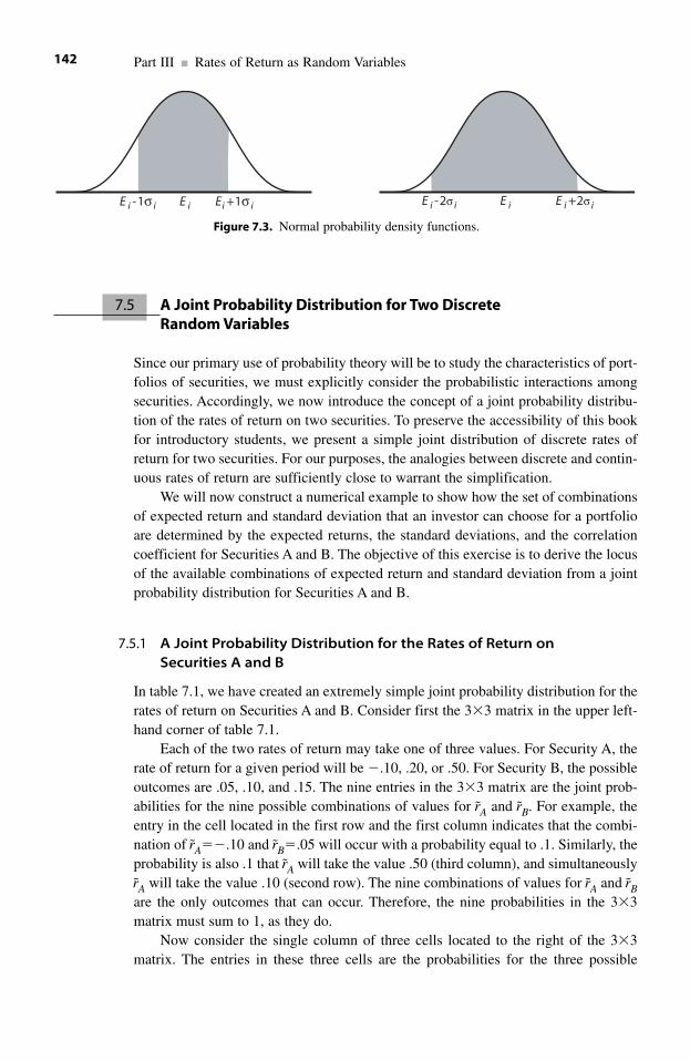
7.5 A Joint Probability Distribution for Two DiscreteRandom Variables

Since our primary use of probability theory will be to study the characteristics of port-folios of securities, we must explicitly consider the probabilistic interactions amongsecurities. Accordingly, we now introduce the concept of a joint probability distribu-tion of the rates of return on two securities. To preserve the accessibility of this bookfor introductory students, we present a simple joint distribution of discrete rates ofreturn for two securities. For our purposes, the analogies between discrete and contin-uous rates of return are sufficiently close to warrant the simplification.

We will now construct a numerical example to show how the set of combinationsof expected return and standard deviation that an investor can choose for a portfolioare determined by the expected returns, the standard deviations, and the correlationcoefficient for Securities A and B. The objective of this exercise is to derive the locusof the available combinations of expected return and standard deviation from a jointprobability distribution for Securities A and B.

7.5.1 A Joint Probability Distribution for the Rates of Return on Securities A and B

In table 7.1, we have created an extremely simple joint probability distribution for therates of return on Securities A and B. Consider first the 3�3 matrix in the upper left-hand corner of table 7.1.

Each of the two rates of return may take one of three values. For Security A, therate of return for a given period will be �.10, .20, or .50. For Security B, the possibleoutcomes are .05, .10, and .15. The nine entries in the 3�3 matrix are the joint prob-abilities for the nine possible combinations of values for rA and rB. For example, theentry in the cell located in the first row and the first column indicates that the combi-nation of rA��.10 and rB�.05 will occur with a probability equal to .1. Similarly, theprobability is also .1 that rA will take the value .50 (third column), and simultaneouslyrA will take the value .10 (second row). The nine combinations of values for rA and rBare the only outcomes that can occur. Therefore, the nine probabilities in the 3�3matrix must sum to 1, as they do.

Now consider the single column of three cells located to the right of the 3�3matrix. The entries in these three cells are the probabilities for the three possible


E i - 2σ i E i + 2σ iE iE i - 1σ i Ei + 1σ iE i

Figure 7.3. Normal probability density functions.

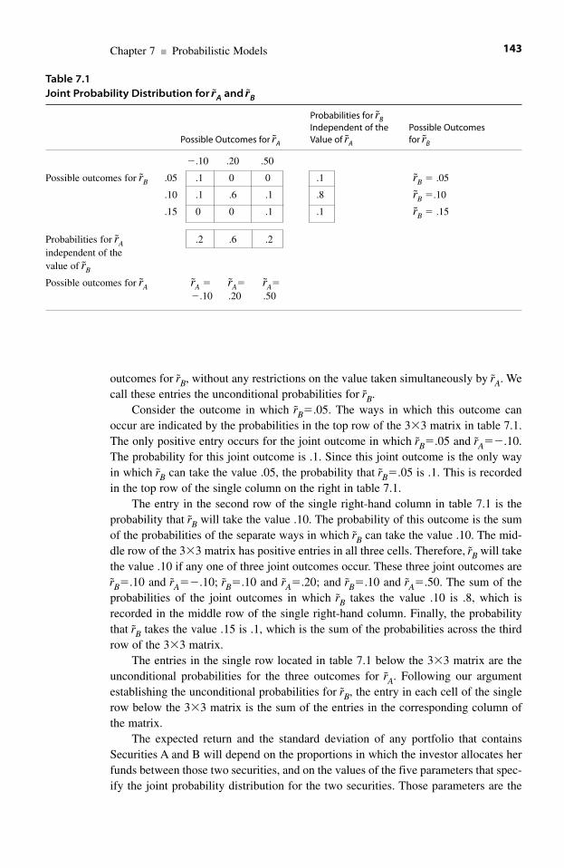
outcomes for rB, without any restrictions on the value taken simultaneously by rA. Wecall these entries the unconditional probabilities for rB.

Consider the outcome in which rB�.05. The ways in which this outcome canoccur are indicated by the probabilities in the top row of the 3�3 matrix in table 7.1.The only positive entry occurs for the joint outcome in which rB�.05 and rA��.10.The probability for this joint outcome is .1. Since this joint outcome is the only wayin which rB can take the value .05, the probability that rB�.05 is .1. This is recordedin the top row of the single column on the right in table 7.1.

The entry in the second row of the single right-hand column in table 7.1 is theprobability that rB will take the value .10. The probability of this outcome is the sumof the probabilities of the separate ways in which rB can take the value .10. The mid-dle row of the 3�3 matrix has positive entries in all three cells. Therefore, rB will takethe value .10 if any one of three joint outcomes occur. These three joint outcomes arerB�.10 and rA��.10; rB�.10 and rA�.20; and rB�.10 and rA�.50. The sum of theprobabilities of the joint outcomes in which rB takes the value .10 is .8, which isrecorded in the middle row of the single right-hand column. Finally, the probabilitythat rB takes the value .15 is .1, which is the sum of the probabilities across the thirdrow of the 3�3 matrix.

The entries in the single row located in table 7.1 below the 3�3 matrix are theunconditional probabilities for the three outcomes for rA. Following our argumentestablishing the unconditional probabilities for rB, the entry in each cell of the singlerow below the 3�3 matrix is the sum of the entries in the corresponding column ofthe matrix.

The expected return and the standard deviation of any portfolio that containsSecurities A and B will depend on the proportions in which the investor allocates herfunds between those two securities, and on the values of the five parameters that spec-ify the joint probability distribution for the two securities. Those parameters are the


Table 7.1Joint Probability Distribution for rA and rB

Probabilities for rBIndependent of the Possible Outcomes

Possible Outcomes for rA Value of rA for rB

�.10 .20 .50

Possible outcomes for rB .05 .1 0 0 .1 rB � .05

.10 .1 .6 .1 .8 rB �.10

.15 0 0 .1 .1 rB � .15

Probabilities for rA .2 .6 .2independent of the value of rB

Possible outcomes for rA rA � rA� rA�

�.10 .20 .50

expected return and the standard deviation of Security A, the expected return and thestandard deviation of Security B, and the correlation coefficient between the rates ofreturn on those securities. Next, we obtain the values of those parameters, beginningwith the expected returns and the standard deviations.

7.5.2 The Expected Returns and the Standard Deviations for Securities A and B

For the joint probability distribution in table 7.1, each security’s rate of return is sym-metrically distributed about its expected value. We can verify this by examining theunconditional distributions that are recorded in the single column to the right of the3�3 matrix and in the single row below that matrix. The column on the right indicatesthat for rB, the lowest and the highest possible outcomes are equidistant from the mid-dle outcome. Moreover, rB will take these two outlying outcomes with equal probabil-ities. Therefore, the expected return for rB is its middle value, .10. Similarly, theexpected return for rA is its middle value, .20.

Recall that the standard deviation is a probability-weighted average of the dis-tances by which the values for a random variable can deviate from its expected value.More precisely, the standard deviation is the positive square root of the probability-weighted average of the squares of distances from the expected value.13

Using the entries in the 3�3 matrix in table 7.1, and the expected values that wehave just calculated for Securities A and B, the value of the standard deviation forSecurity A is:

Similarly, the value of the standard deviation for Security B is:

Note that the standard deviation for Security A is larger than the standard deviation forSecurity B. There are two reasons for this. First, the distance from EA to either of the twooutlying values for rA is greater than the distance from EB to either of the two outlyingvalues for rB. Second, the probabilities that rA will take either of its outlying values aregreater than the probabilities that rB will take either of its outlying values.

�

� � �

�

�

�

B B2

2 2[( .05) (.1) (.05) (.1)]

2(.1)(.0025)

(.2)(.0025)

.00005

.0224.�

�

� � � � � � �

� �

A A2

2 2 2[( .10 .20) (.2) (.20 .20) (.6) (.50 .20) (.2)]

[( ..30) (.2) (0) (.6) (.30) (.2)]

[2(.2)(.09)]

.036

.1897.

2 2 2� �

�

�

�


(7.10)

(7.11)

7.5.3 The Covariance and the Correlation Coefficient between the Rates of Return on Securities A and B

To develop portfolio theory in chapter 8, we need two additional parameters. Theseare the covariance and the correlation coefficient between the rates of return onSecurities A and B. The covariance is the probability-weighted sum of all possibleproducts of deviations of the rates of return on Securities A and B from theexpected values for those securities. The correlation coefficient between the ratesof return on Security A and B is equal to the covariance between those securitiesdivided by the product of their standard deviations. The correlation coefficient is,therefore, a scaled covariance. The effect of the scaling is to restrict the possiblevalues for the correlation coefficient to the interval from �1 to �1, including theendpoints.

We begin with the covariance. The covariance between any two random vari-ables is the probability-weighted average of the products of the distances by whicheach random variable can deviate from its expected return. To calculate the covari-ance between rA and rB, we must first identify all the possible combinations of thedeviations that the two random variables can take from their expected returns.Define CAB as the covariance between the rates of return on Securities A and B. Thejoint probability distribution for rA and rB specified in table 7.1 is so simple thatthere are only two terms in the calculation of CAB. These terms are generated by thecell in the top row of the first column and by the cell in the bottom row of the thirdcolumn.

We can ignore the four cells whose entries are zero. Since CAB is a probability-weighted average, the combinations of outcomes corresponding to these four cells donot enter the calculation of CAB. We can also ignore the entire middle row of table 7.1.The covariance involves products of deviations from expected returns. The entiremiddle row of table 7.1 pertains to the three outcomes in which rB takes the value ofits expected return. Therefore, the deviation of rB from EB is equal to zero for each ofthese three outcomes. Consequently, for each of the outcomes corresponding to themiddle row of table 7.1, the products of the deviations from the expected returns willbe equal to zero.

Now that we have eliminated from consideration all but the cells in the upper leftand the lower right corners of the matrix in table 7.1, we can calculate the covariancebetween rA and rB as:

(7.12)

The value of the covariance between rA and rB depends on the combinations ofthe deviations of rA from EA and rB from EB. If both random variables frequently takevalues on the same sides of their respective expected values, the covariance will bepositive. The joint probabilities in table 7.1 indicate that rA and rB cannot simultane-ously take values on opposite sides of their expected returns. Therefore, CAB must bepositive. The value of CAB is quite small because the probabilities of the possible devi-ations are small.

CAB � � � � � � �

� �

(.1)( .10 .20)(.05 .10) (.1)(.50 .20)(.15 .10)

(.1)( .330)( .05) (.1)(.30)(.05)

.003.

� �

�


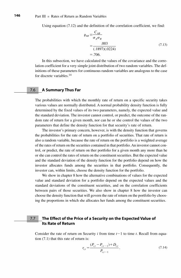
Using equation (7.12) and the definition of the correlation coefficient, we find:

(7.13)

In this subsection, we have calculated the values of the covariance and the corre-lation coefficient for a very simple joint distribution of two random variables. The def-initions of these parameters for continuous random variables are analogous to the casefor discrete variables.14

7.6 A Summary Thus Far

The probabilities with which the monthly rate of return on a specific security takesvarious values are normally distributed. A normal probability density function is fullydetermined by the fixed values of its two parameters, namely, the expected value andthe standard deviation. The investor cannot control, or predict, the outcome of the ran-dom rate of return for a given month, nor can he or she control the values of the twoparameters that define the density function for that security’s rate of return.

The investor’s primary concern, however, is with the density function that governsthe probabilities for the rate of return on a portfolio of securities. That rate of return isalso a random variable, because the rate of return on the portfolio is a weighted averageof the rates of return on the securities contained in that portfolio. An investor cannot con-trol, or predict, the rate of return on ther portfolio for a given month any more than heor she can control the rates of return on the constituent securities. But the expected valueand the standard deviation of the density function for the portfolio depend on how theinvestor allocates funds among the securities in that portfolio. Consequently, theinvestor can, within limits, choose the density function for the portfolio.

We show in chapter 8 how the alternative combinations of values for the expectedvalue and standard deviation for a portfolio depend on the expected values and thestandard deviations of the constituent securities, and on the correlation coefficientsbetween pairs of those securities. We also show in chapter 8 how the investor canchoose the density function that will govern the rate of return on the portfolio by choos-ing the proportions in which she allocates her funds among the constituent securities.

7.7 The Effect of the Price of a Security on the Expected Value of Its Rate of Return

Consider the rate of return on Security i from time t�1 to time t. Recall from equa-tion (7.1) that this rate of return is:

(7.14)rP P D

Pi ti t i t i t

i t,

, , 1 ,

, 1

( ).�

� ��

�

�

�

�

ABAB

A B

C≡

.003

(.1897)(.0224)

.706.


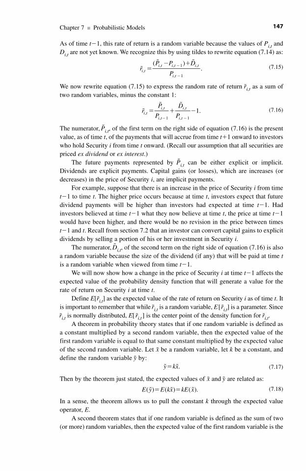
As of time t�1, this rate of return is a random variable because the values of Pi,t andDi,t are not yet known. We recognize this by using tildes to rewrite equation (7.14) as:

(7.15)

We now rewrite equation (7.15) to express the random rate of return ri,t as a sum oftwo random variables, minus the constant 1:

(7.16)

The numerator, Pi,t, of the first term on the right side of equation (7.16) is the presentvalue, as of time t, of the payments that will accrue from time t�1 onward to investorswho hold Security i from time t onward. (Recall our assumption that all securities arepriced ex dividend or ex interest.)

The future payments represented by Pi,t can be either explicit or implicit.Dividends are explicit payments. Capital gains (or losses), which are increases (ordecreases) in the price of Security i, are implicit payments.

For example, suppose that there is an increase in the price of Security i from timet�1 to time t. The higher price occurs because at time t, investors expect that futuredividend payments will be higher than investors had expected at time t�1. Hadinvestors believed at time t�1 what they now believe at time t, the price at time t�1would have been higher, and there would be no revision in the price between timest�1 and t. Recall from section 7.2 that an investor can convert capital gains to explicitdividends by selling a portion of his or her investment in Security i.

The numerator, Di,t, of the second term on the right side of equation (7.16) is alsoa random variable because the size of the dividend (if any) that will be paid at time tis a random variable when viewed from time t�1.

We will now show how a change in the price of Security i at time t�1 affects theexpected value of the probability density function that will generate a value for therate of return on Security i at time t.

Define E[ri,t] as the expected value of the rate of return on Security i as of time t. Itis important to remember that while ri,t is a random variable, E[ ri,t] is a parameter. Sinceri,t is normally distributed, E[ ri,t ] is the center point of the density function for ri,t.

A theorem in probability theory states that if one random variable is defined asa constant multiplied by a second random variable, then the expected value of thefirst random variable is equal to that same constant multiplied by the expected valueof the second random variable. Let x be a random variable, let k be a constant, anddefine the random variable y by:

(7.17)

Then by the theorem just stated, the expected values of x and y are related as:

(7.18)

In a sense, the theorem allows us to pull the constant k through the expected valueoperator, E.

A second theorem states that if one random variable is defined as the sum of two(or more) random variables, then the expected value of the first random variable is the

E y E kx kE x( ) ( ) ( ).� � ��

� �y kx� .

�

� �

rP

P

D

Pi ti t

i t

i t

i t,

,

, 1

,

, 1

1.� � ��

�

� �

rP P D

Pi ti t i t i t

i t,

, , 1 ,

, 1

( )�

� ��

�

.


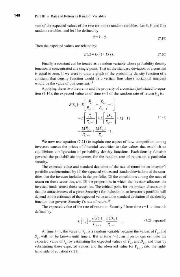
sum of the expected values of the two (or more) random variables. Let x , y, and z berandom variables, and let z be defined by:

(7.19)

Then the expected values are related by:

(7.20)

Finally, a constant can be treated as a random variable whose probability densityfunction is concentrated at a single point. That is, the standard deviation of a constantis equal to zero. If we were to draw a graph of the probability density function of aconstant, that density function would be a vertical line whose horizontal interceptwould be the value of that constant.15

Applying these two theorems and the property of a constant just stated to equa-tion (7.16), the expected value as of time t�1 of the random rate of return ri,t is:

We now use equation (7.21) to explain one aspect of how competition amonginvestors causes the prices of financial securities to take values that establish anequilibrium configuration of probability density functions. Each density functiongoverns the probabilistic outcomes for the random rate of return on a particularsecurity.

The expected value and standard deviation of the rate of return on an investor’sportfolio are determined by (1) the expected values and standard deviations of the secu-rities that the investor includes in the portfolio, (2) the correlations among the rates ofreturn on those securities, and (3) the proportions in which the investor allocates theinvested funds across those securities. The critical point for the present discussion isthat the attractiveness of a given Security i for inclusion in an investor’s portfolio willdepend on the estimates of the expected value and the standard deviation of the densityfunction that governs Security i’s rate of return.16

The expected value of the rate of return on Security i from time t�1 to time t isdefined by:

(7.21, repeated)

At time t�1, the value of ri,t is a random variable because the values of Pi,t andDi,t will not be known until time t. But at time t�1, an investor can estimate theexpected value of ri,t by estimating the expected values of Pi,t and Di,t, and then bysubstituting these expected values, and the observed value for Pi,t-1, into the right-hand side of equation (7.21).

E rE P

P

E D

Pi ti t

i t

i t

i t

�

� �

,,

, 1

,

, 1

( ) ( )1.⎡⎣ ⎤⎦� � �

� �

E r EP

P

D

P

EP

P

i ti t

i t

i t

i t

i t

i t

[ ] 1,,

, 1

,

, 1

,

, 1

�

� �

�

� � �

�

� �

�

⎡

⎣⎢⎢

⎤

⎦⎥⎥

⎡

⎣⎢⎢⎢

⎤

⎦⎥⎥

⎡

⎣⎢⎢

⎤

⎦⎥⎥

� � �

� �

�

�

ED

PE

E P

P

E D

i t

i t

i t

i t

i t

�

� �

,

, 1

,

, 1

,

[ 1]

[ ] [ ]

PPi t,

1.�

E z E x E y( ) ( ) ( ).� � ��

� � �z x y� � .


(7.21)

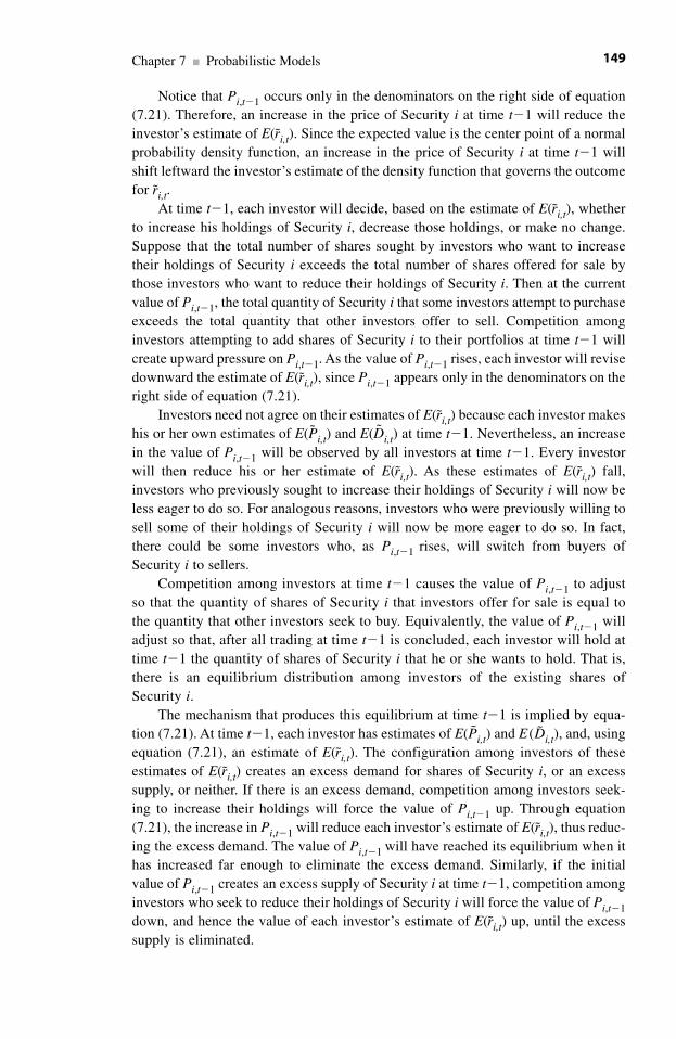
Notice that Pi,t�1 occurs only in the denominators on the right side of equation(7.21). Therefore, an increase in the price of Security i at time t�1 will reduce theinvestor’s estimate of E(ri,t). Since the expected value is the center point of a normalprobability density function, an increase in the price of Security i at time t�1 willshift leftward the investor’s estimate of the density function that governs the outcomefor ri,t.

At time t�1, each investor will decide, based on the estimate of E(ri,t), whetherto increase his holdings of Security i, decrease those holdings, or make no change.Suppose that the total number of shares sought by investors who want to increasetheir holdings of Security i exceeds the total number of shares offered for sale bythose investors who want to reduce their holdings of Security i. Then at the currentvalue of Pi,t�1, the total quantity of Security i that some investors attempt to purchaseexceeds the total quantity that other investors offer to sell. Competition amonginvestors attempting to add shares of Security i to their portfolios at time t�1 willcreate upward pressure on Pi,t�1. As the value of Pi,t�1 rises, each investor will revisedownward the estimate of E(ri,t), since Pi,t�1 appears only in the denominators on theright side of equation (7.21).

Investors need not agree on their estimates of E(ri,t) because each investor makeshis or her own estimates of E(Pi,t) and E(Di,t) at time t�1. Nevertheless, an increasein the value of Pi,t�1 will be observed by all investors at time t�1. Every investorwill then reduce his or her estimate of E(ri,t). As these estimates of E(ri,t) fall,investors who previously sought to increase their holdings of Security i will now beless eager to do so. For analogous reasons, investors who were previously willing tosell some of their holdings of Security i will now be more eager to do so. In fact,there could be some investors who, as Pi,t�1 rises, will switch from buyers ofSecurity i to sellers.

Competition among investors at time t�1 causes the value of Pi,t�1 to adjustso that the quantity of shares of Security i that investors offer for sale is equal tothe quantity that other investors seek to buy. Equivalently, the value of Pi,t�1 willadjust so that, after all trading at time t�1 is concluded, each investor will hold attime t�1 the quantity of shares of Security i that he or she wants to hold. That is,there is an equilibrium distribution among investors of the existing shares ofSecurity i.

The mechanism that produces this equilibrium at time t�1 is implied by equa-tion (7.21). At time t�1, each investor has estimates of E(Pi,t) and E (Di,t), and, usingequation (7.21), an estimate of E(ri,t). The configuration among investors of theseestimates of E(ri,t) creates an excess demand for shares of Security i, or an excesssupply, or neither. If there is an excess demand, competition among investors seek-ing to increase their holdings will force the value of Pi,t�1 up. Through equation(7.21), the increase in Pi,t�1 will reduce each investor’s estimate of E(ri,t), thus reduc-ing the excess demand. The value of Pi,t�1 will have reached its equilibrium when ithas increased far enough to eliminate the excess demand. Similarly, if the initialvalue of Pi,t�1 creates an excess supply of Security i at time t�1, competition amonginvestors who seek to reduce their holdings of Security i will force the value of Pi,t�1down, and hence the value of each investor’s estimate of E(ri,t) up, until the excesssupply is eliminated.


7.8 The Effect of the Price of a Security on the Standard Deviation of Its Rate of Return

The standard deviation of a random variable is the positive square root of the varianceof that random variable. For some purposes, it is more convenient to work with thevariance.

Repeating equation (7.16), the rate of return is

(7.22)

The rate of return for Security i is equal to the sum of two random variables, eachof which is multiplied by the constant 1/Pi,t�1, minus a constant. To calculate the vari-ance of ri,t, we use the following property of the variance of a sum of random vari-ables. Let x, y, and z be random variables, and define the random variable w by:

(7.23)

in which a, b, and c are constants. Then

(7.24)

in which Cx y is the covariance between x and y, and Cyz and Cxz are defined similarly.Defining a�b�1/Pi,t�1, c�1, and z�1, and applying (7.24) to (7.22), we may writethe variance of the rate of return on Security i as:

(7.25)

In obtaining (7.25), we used the facts that the variance of z and any covarianceinvolving z are zero. This is true because every term in a variance, and every term ina covariance, is a deviation of the value of a random variable from its expected value.Sinze z is a constant (equal to 1), when we apply (7.24) to (7.23), every term in thevariance of z, and every term in any covariance between z and any other random vari-able, is equal to zero.

We conclude from (7.25) that the effect on the variance of ri,t of a change in Pi,t�1is ambiguous because the covariance (CPi,t,Di,t), between the price and the dividend attime t, can be either positive or negative.

7.9 A Linear Model of the Rate of Return

To prepare for work on portfolio theory in chapter 8, and on capital market theory inchapters 9 and 10, we present here a linear probabilistic model for the rate of return ona security. The central idea is that as the rate of return on a special portfolio changesfrom one period to the next, the probability density function for the rate of return onSecurity i shifts rightward or leftward along the horizontal axis in figure 7.1. Usually,this special portfolio is constructed so that it represents either the entire economy orsome sector of the economy. Consequently, the coefficient in the linear equation that

� � �

� �

�

�

� � � �

r

P D P D

i ti t

i t i t i t i tC

P,

, , , 1 , 12

2 2,

, 12

2

( )

� � �

� � �

� � � �

� � � � � �

w y z

x y x z y z

a b c

abC acC bcC

2 2 2 2 2 2 2

, , ,2 2 2

x

� � � �w ax by cz� � � ,

�

� �

rP

P

D

Pi ti t

i t

i t

i t,

,

, 1

,

, 1

1.� � ��


determines the expected value for the rate of return on Security i measures the sensi-tivity of the probability density function for the rate of return on Security i to changesin the level of macroeconomic activity.

The model that we present is an amplification of the model that we sketchedtoward the end of chapter 6. In chapters 8, 9, and 10, we discuss alternatives for con-structing this portfolio. In fact, the various asset pricing models are distinguished bythe structure of the portfolio, or portfolios, whose rates of return at time t locate theexpected value of the density function for the rate of return on Security i.

7.9.1 Conditional Density Functions

A portfolio is a collection of securities. Suppose that Portfolio M contains 100 secu-rities, and let j be an index that takes any of the values 1, 2, . . . , 100. Assigning oneof these values to j specifies a particular security in Portfolio M. When we speak in general of Security j, we are making a statement that applies to any of the 100 securities.

Portfolio M has a rate of return that is derived from the rates of return of its con-stituent securities. If the rates of return on these securities are normally distributed,then the portfolio’s rate of return will also be normally distributed. In fact, theexpected value and standard deviation of the portfolio’s density function will be deter-mined by (1) the expected values and standard deviations of the rates of return on theconstituent securities, (2) the correlation coefficients among those rates of return, and(3) the proportions in which the portfolio’s total funds are allocated among those con-stituent securities. We explain this relationship in more detail in chapter 8.

Let Security i be any security. Security i might, or might not, be a member ofPortfolio M. Let rm,t be the rate of return on Portfolio M for time t.

Consider the following linear model. For any time t, the rate of return on Securityi is generated by:

(7.26)

In equation (7.26), the terms i and �i are constants specific to Security i. The term�i is a random variable that is specific to Security i.

We impose two restrictions on the model in equation (7.26). First, we require thatfor all securities, �i is normally distributed and has an expected value equal to zero.Then:

(7.27)

Second, we require that the random variables rM and �i are independent for allsecurities. We discuss the meaning of independence between random variables inmore detail in section 7.12 on correlation. For now, it is sufficient to state that inde-pendence between rm and �i means that an outcome for either random variable has noinfluence on the probabilities with which the other random variable will take specificvalues.

The model in equation (7.26) asserts that the rate of return on Security i dependson two sets of forces. One set of forces is generated by the behavior of the macroecon-omy in which Firm i does business. For example, the general level of interest rates,the rate of inflation, whether consumers fear the onset of a recession, the level and the

E i ii( ) 0 for all Securities , 1,2, . . . ,100.��

� � �r ri t i i m i, .� � ��α β


structure of corporate and personal income taxes, and the levels of prices in financialmarkets will affect the ability of Firm i to generate earnings. The model in equation(7.26) uses the value of rm,t as an index of the state of the economy in which Firm ioperates. Note that the subscript i on the coefficient �i in equation (7.26) indicates thata change in the state of the economy, as measured by a change in the value of rm,t, willnot affect all firms equally. The effect on ri,t of a change in rm,t will depend on theparameter �i, which is specific to Firm i. If Firm i’s rate of return is highly sensitiveto the state of the macroeconomy, then the value of �i will be large and postive.17

The second set of forces that affect ri,t is specific to Firm i. These forces include,for example, variations in the efficiency of the firm’s management, progress or delaysin bringing the firm’s new products to market, favorable or unfavorable resolution oflawsuits involving the firm, changes in the costs of the firm’s inputs, and changes inthe strategies employed by the firm’s competitors. These forces are called firm-specific or idiosyncratic forces. Their effects on ri,t are transmitted through �i.

At any time t, the effect of the firm-specific forces on ri,t may be either positiveor negative. These effects are random. Thus the outcome for �i at any time t ismodeled as an outcome from a normal density function. For analytical and graphical convenience, we define �i so that E(�i)�0.

The constant �i is that part of Firm i’s average rate of return that does not dependon the state of the macroeconomy. For example, if Firm i is in a sector of the econ-omy that investors expect to have rapid growth of earnings, such as Internet firms,then the value of �i will be large. If the expected value of the firm-specific term, �i,were nonzero, we would incorporate this expected value of �i into the value of �i andthen redefine �i so that its expected value is zero.

Reading from left to right in equation (7.26), for any time t, the rate of return onSecurity i is equal to �i adjusted by two disturbances. The value of the macroeco-nomic disturbance is �irm,t and the value of the microeconomic (or firm-specific) dis-turbance is �i,t. We can interpret this model easily by presenting it graphically as aprobability density function for Security i that shifts rightward or leftward withchanges in the level of macroeconomic activity. The value of the sensitivity coeffi-cient for Security i, �i, determines the distance by which a change in the level ofmacroeconomic activity shifts the density function for Security i.

Suppose that at time t the outcome for the rate of return on Portfolio M is the par-ticular value rA. Then the only variability in ri,t will be caused by the random outcomefor the firm-specific disturbance �i. Note the absence of a subscript t on the randomvariable �i. The probability density function for �i does not shift from one time to thenext. With the outcome for rm,t fixed at rA, the outcome for ri,t will be the sum of theconstants �i and �irA, plus the random outcome for �i. Using the theorems forexpected value, and our assumption that E(�i)�0, the expected value for ri,t, given thatrm,t has taken the value rA, is

(7.28)

The symbol E(ri,t |rm,t�rA) is read as “the conditional expected value of (the randomvariable) ri,t, under the condition that (the random variable) rm,t takes the value rA. The

E r r r

r E

r

i t m t A

i A i

i i A

( )

( )

.

, ,� �

�

⏐ �

��

��

i


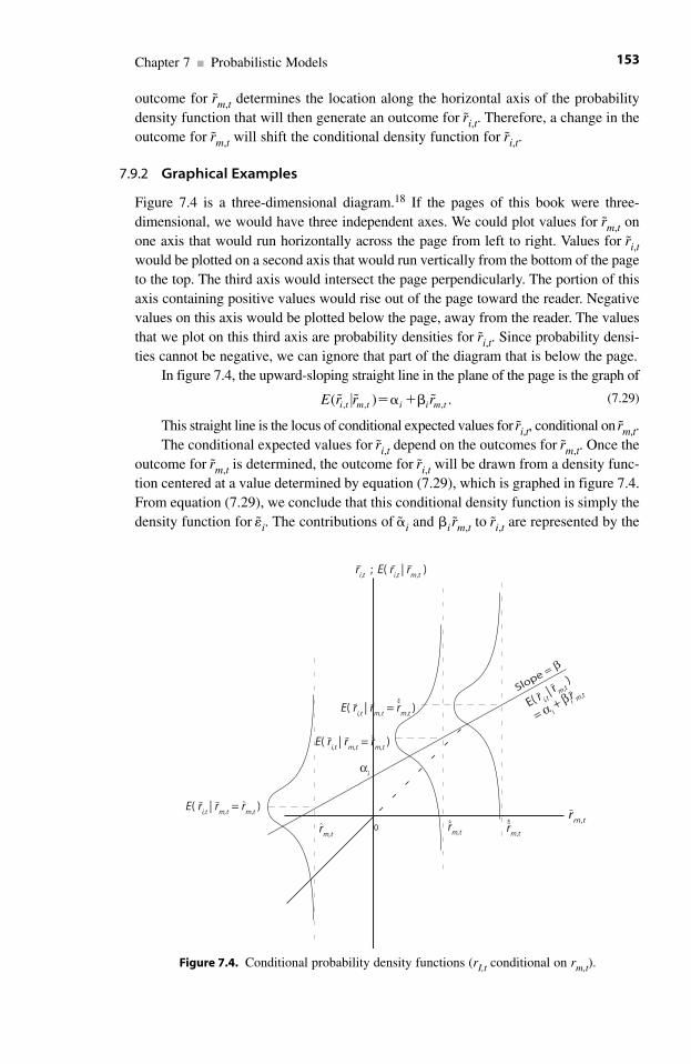
outcome for rm,t determines the location along the horizontal axis of the probabilitydensity function that will then generate an outcome for ri,t. Therefore, a change in theoutcome for rm,t will shift the conditional density function for ri,t.

7.9.2 Graphical Examples

Figure 7.4 is a three-dimensional diagram.18 If the pages of this book were three-dimensional, we would have three independent axes. We could plot values for rm,t onone axis that would run horizontally across the page from left to right. Values for ri,twould be plotted on a second axis that would run vertically from the bottom of the pageto the top. The third axis would intersect the page perpendicularly. The portion of thisaxis containing positive values would rise out of the page toward the reader. Negativevalues on this axis would be plotted below the page, away from the reader. The valuesthat we plot on this third axis are probability densities for ri,t. Since probability densi-ties cannot be negative, we can ignore that part of the diagram that is below the page.

In figure 7.4, the upward-sloping straight line in the plane of the page is the graph of

(7.29)

This straight line is the locus of conditional expected values for ri,t, conditional on rm,t.The conditional expected values for ri,t depend on the outcomes for rm,t. Once the

outcome for rm,t is determined, the outcome for ri,t will be drawn from a density func-tion centered at a value determined by equation (7.29), which is graphed in figure 7.4.From equation (7.29), we conclude that this conditional density function is simply thedensity function for �i. The contributions of �i and �i rm,t to ri,t are represented by the

E r r ri t m t i i m t( ) ., , ,� � �⏐ ��


rm,t

Slope = β

ri,t

; E( ri,t

| rm,t

)

E( r i,t| r m,t

)

= α i + β i

r m,t

rm,t

rm,t

rm,t

0

αi

E( ri,t

| rm,t

= rm,t

)

E( ri,t

| rm,t

= rm,t

)

E( ri,t

| rm,t

= rm,t

)

Figure 7.4. Conditional probability density functions (rI,t conditional on rm,t).

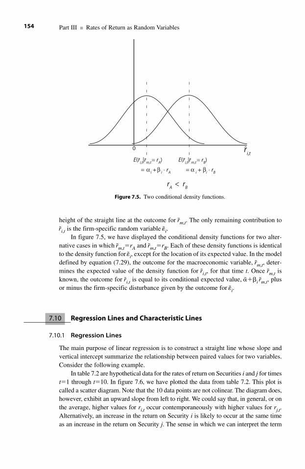
height of the straight line at the outcome for rm,t. The only remaining contribution tori,t is the firm-specific random variable �i.

In figure 7.5, we have displayed the conditional density functions for two alter-native cases in which rm,t�rA and rm,t�rB. Each of these density functions is identicalto the density function for �i, except for the location of its expected value. In the modeldefined by equation (7.29), the outcome for the macroeconomic variable, rm,t, deter-mines the expected value of the density function for ri,t, for that time t. Once rm,t isknown, the outcome for ri,t is equal to its conditional expected value, ��i rm,t, plusor minus the firm-specific disturbance given by the outcome for �i.

7.10 Regression Lines and Characteristic Lines

7.10.1 Regression Lines

The main purpose of linear regression is to construct a straight line whose slope andvertical intercept summarize the relationship between paired values for two variables.Consider the following example.

In table 7.2 are hypothetical data for the rates of return on Securities i and j for timest�1 through t�10. In figure 7.6, we have plotted the data from table 7.2. This plot iscalled a scatter diagram. Note that the 10 data points are not colinear. The diagram does,however, exhibit an upward slope from left to right. We could say that, in general, or onthe average, higher values for ri,t occur contemporaneously with higher values for rj,t.Alternatively, an increase in the return on Security i is likely to occur at the same timeas an increase in the return on Security j. The sense in which we can interpret the term


rA

< rB

ri,t

= α βi + i · rA

E(ri,t|rm,t= rA)

= α i + βi · rB

E(ri,t|rm,t= rB)

0

Figure 7.5. Two conditional density functions.

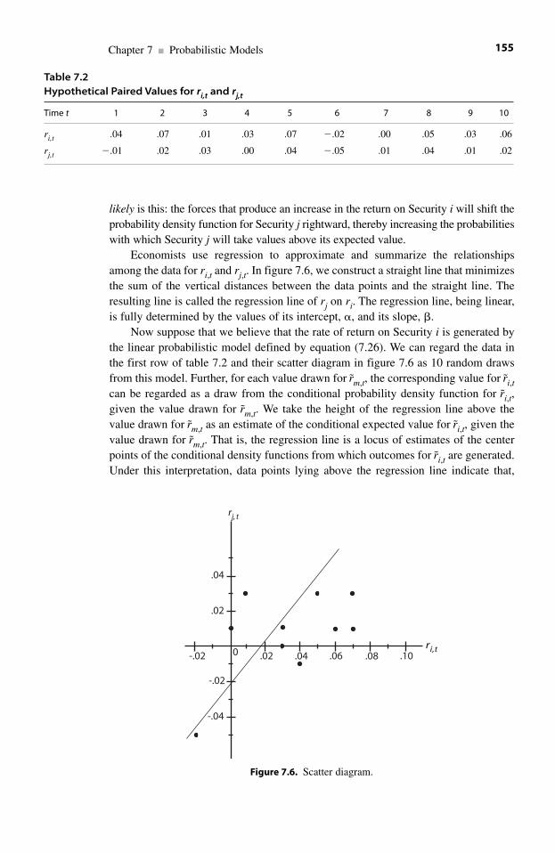
likely is this: the forces that produce an increase in the return on Security i will shift theprobability density function for Security j rightward, thereby increasing the probabilitieswith which Security j will take values above its expected value.

Economists use regression to approximate and summarize the relationshipsamong the data for ri,t and rj,t. In figure 7.6, we construct a straight line that minimizesthe sum of the vertical distances between the data points and the straight line. Theresulting line is called the regression line of rj on ri. The regression line, being linear,is fully determined by the values of its intercept, �, and its slope, �.

Now suppose that we believe that the rate of return on Security i is generated bythe linear probabilistic model defined by equation (7.26). We can regard the data inthe first row of table 7.2 and their scatter diagram in figure 7.6 as 10 random drawsfrom this model. Further, for each value drawn for rm,t, the corresponding value for ri,tcan be regarded as a draw from the conditional probability density function for ri,t,given the value drawn for rm,t. We take the height of the regression line above thevalue drawn for rm,t as an estimate of the conditional expected value for ri,t, given thevalue drawn for rm,t. That is, the regression line is a locus of estimates of the centerpoints of the conditional density functions from which outcomes for ri,t are generated.Under this interpretation, data points lying above the regression line indicate that,


Table 7.2Hypothetical Paired Values for ri,t and rj,t

Time t 1 2 3 4 5 6 7 8 9 10

ri,t .04 .07 .01 .03 .07 �.02 .00 .05 .03 .06

rj,t �.01 .02 .03 .00 .04 �.05 .01 .04 .01 .02

ri,t

rj, t

.06-.02

-.02

-.04

.04

.02

0 .02 .04 .10.08

Figure 7.6. Scatter diagram.

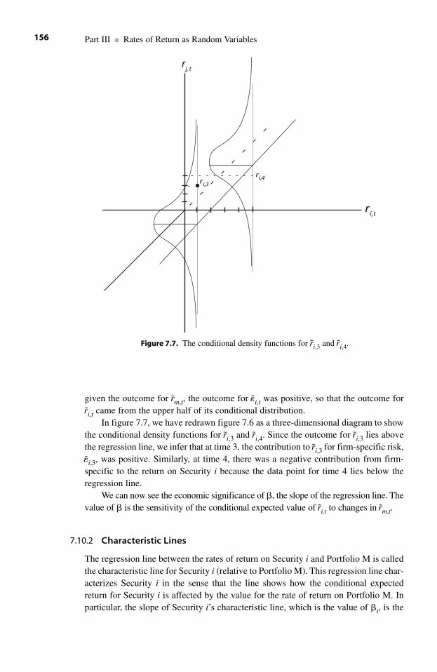
given the outcome for rm,t, the outcome for �i,t was positive, so that the outcome forri,t came from the upper half of its conditional distribution.

In figure 7.7, we have redrawn figure 7.6 as a three-dimensional diagram to showthe conditional density functions for ri,3 and ri,4. Since the outcome for ri,3 lies abovethe regression line, we infer that at time 3, the contribution to ri,3 for firm-specific risk,�i,3, was positive. Similarly, at time 4, there was a negative contribution from firm-specific to the return on Security i because the data point for time 4 lies below theregression line.

We can now see the economic significance of �, the slope of the regression line. Thevalue of � is the sensitivity of the conditional expected value of ri,t to changes in rm,t.

7.10.2 Characteristic Lines

The regression line between the rates of return on Security i and Portfolio M is calledthe characteristic line for Security i (relative to Portfolio M). This regression line char-acterizes Security i in the sense that the line shows how the conditional expectedreturn for Security i is affected by the value for the rate of return on Portfolio M. Inparticular, the slope of Security i’s characteristic line, which is the value of �i, is the


ri,t

ri,3

ri,4

rj, t

Figure 7.7. The conditional density functions for ri,3 and ri,4.

rate at which the conditional density function for Security i will shift whenever therate of return on Portfolio M increases by one percentage point.

7.11 The Parameter �i as the Quantity of Risk in Security i

As we sketched in chapter 6 and show in chapters 9 and 10, the value of �i is the quan-tity of risk contained in Security i. Here is a brief statement of the rationale that sup-ports this interpretation of �i.

A central objective of portfolio theory is to explain how an investor should allo-cate funds among individual securities to create a portfolio that will maximize theexpected rate of return, given a fixed level of risk in that portfolio. In chapter 8, weshow that an equivalent objective is to minimize the level of risk in the portfolio,given a fixed level of expected return. Of course, each of these objectives requires thatwe specify how risk is to be measured.

The measurement of risk will occupy much of our attention in chapter 8. Therewe explain why economists measure the level of risk in a portfolio as the standarddeviation of the rate of return on that portfolio. The measure of risk for an individualsecurity is more complicated, but the reasoning is both clear and persuasive. We showthat a prudent investor will allocate funds across a diversified portfolio of securities,rather than placing all funds in a single security. Therefore, we measure the level ofrisk that an investor bears by holding any particular security by the effect of that secu-rity on the standard deviation of the portfolio in which the investor holds that security.This contribution from portfolio theory is the basis for capital market theory, whichgenerates hypotheses about the equilibrium relationship between the level of risk in asecurity and the expected value of its rate of return.

In chapter 8, we show that the standard deviation of a portfolio is equal to aweighted sum of the beta values of its constituent securities. The weights in this sumdepend on the proportions in which the investor allocates funds across the securitiesin the portfolio. Consequently, the level of risk that an investor incurs by includingSecurity i in his or her portfolio is proportional to the value of Security i’s beta.Further, the marginal effect of Security i on the standard deviation of the portfolio isproportional to the �i. The higher the value of a security’s beta, the more volatile willbe a portfolio in which that security is held. Therefore, the higher the beta for anySecurity i, the lower must be the price of Security i if an investor is to include thatsecurity in the portfolio.

When the word risk is introduced into a discussion of investments and financialmarkets, some students think of an outcome in which the investor loses all, or sub-stantially all, of the investment. However, as we show in the next chapter, there arestrong reasons to believe that an investor who holds a properly diversified portfoliofaces a negligible probability of losing the entire investment, or even most of it.19

The more significant risk for an investor is the volatility of the rate of return onthe portfolio. Consider an investor who depends on investments to generate income tomeet current obligations.20 This investor might be a retired person who is relying on


investment income to meet living expenses. Alternatively, the investor might be a col-lege, a hospital, or a charity such as the Salvation Army, whose trustees rely on invest-ment income to meet some of their regular, ongoing expenses. All of these investorscould be harmed if the rates of return on their investments were highly, and unpre-dictably, volatile.

Investors who do not rely on their investments to generate current income are lesssensitive to unpredictable volatility, but they are not indifferent to it. Consider theinvestor who is trying to accumulate capital to finance a child’s education at collegeor the construction of a retirement home. This investor can tolerate variations in therate of return from one year to the next, especially in the early years. But the widerthe fluctuations in the rates of return, and the higher the probability of an extendedsequence of low rates of return, the higher is the risk that the investor will not haveaccumulated sufficient capital to send his daughter to college or to build his retirementhome.

For all of these reasons, investors are sensitive to the volatility in the rate of returnon their portfolios. In the next chapter, we explain in detail how the probabilisticbehaviors of the rates of return on individual securities interact to determine thevolatility of the rate of return on the portfolio in which an investor holds those secu-rities. Then in chapter 9, on capital market theory, we explain how economists use therelationship between individual securities and portfolios to create a model of thetrade-off that financial markets will establish between the expected return and the riskon individual securities. This model, the capital asset pricing model, is one of the sem-inal contributions to the economics of financial markets.

7.12 Correlation

7.12.1 General Observations

The regression line in figure 7.6 is the straight line that best fits the scatter diagramaccording to the criterion of minimizing the sum of (squared) vertical deviations fromthe data points to the regression line. Correlation is a measure of how closely the datapoints are distributed above and below the regression line. For an initial glance at thedifference between correlation and regression, consider figure 7.8. Although the datapoints in (b) are more widely dispersed than those in (a), both scatter diagrams haveidentical regression lines. The two scatter diagrams are constructed so that the straightline that best fits the data in (a) has the same pair of values for its slope and interceptas the line that best fits the data in (b).21

The two scatter diagrams differ in the average proximity of their data points totheir regression lines. The correlation coefficient for a set of data points is a measureof the average proximity of the data points to their regression line. Sometimes, thecorrelation coefficient is described as a measure of closeness of fit.

By definition, the correlation coefficient takes a value between �1 and �1. Fora given scatter diagram, the sign of the correlation coefficient will be the same as thesign of the slope of the regression line for that scatter diagram. The more closely the


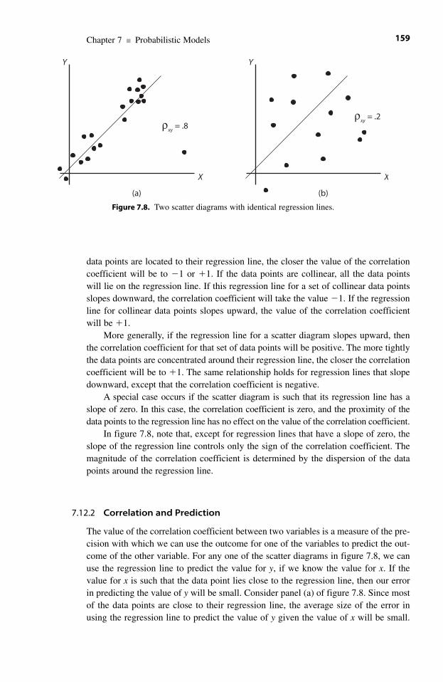
data points are located to their regression line, the closer the value of the correlationcoefficient will be to �1 or �1. If the data points are collinear, all the data points will lie on the regression line. If this regression line for a set of collinear data pointsslopes downward, the correlation coefficient will take the value �1. If the regressionline for collinear data points slopes upward, the value of the correlation coefficientwill be �1.

More generally, if the regression line for a scatter diagram slopes upward, thenthe correlation coefficient for that set of data points will be positive. The more tightlythe data points are concentrated around their regression line, the closer the correlationcoefficient will be to �1. The same relationship holds for regression lines that slopedownward, except that the correlation coefficient is negative.

A special case occurs if the scatter diagram is such that its regression line has aslope of zero. In this case, the correlation coefficient is zero, and the proximity of thedata points to the regression line has no effect on the value of the correlation coefficient.

In figure 7.8, note that, except for regression lines that have a slope of zero, theslope of the regression line controls only the sign of the correlation coefficient. Themagnitude of the correlation coefficient is determined by the dispersion of the datapoints around the regression line.

7.12.2 Correlation and Prediction

The value of the correlation coefficient between two variables is a measure of the pre-cision with which we can use the outcome for one of the variables to predict the out-come of the other variable. For any one of the scatter diagrams in figure 7.8, we canuse the regression line to predict the value for y, if we know the value for x. If thevalue for x is such that the data point lies close to the regression line, then our errorin predicting the value of y will be small. Consider panel (a) of figure 7.8. Since mostof the data points are close to their regression line, the average size of the error inusing the regression line to predict the value of y given the value of x will be small.


Y

X

(a)

ρxy

= .8

Y

X

(b)

ρxy

= .2

Figure 7.8. Two scatter diagrams with identical regression lines.

Analogously, if the data points are widely dispersed around their regression line, as inpanel (b), then the average error will be large.

For any scatter diagram, the absolute value of its correlation coefficient is deter-mined by the dispersion of the data points around their regression line. Therefore, theabsolute value of the correlation coefficient is a measure of the value of knowing theslope and the vertical intercept of the regression line if one is interested in using the value of x to predict the value of y. For example, if we wanted to predict y from x,and we knew that the absolute value of the correlation coefficient is high, as in panel (a), then we would be willing to pay a higher price to discover the equation ofthe regression line than we would if the absolute value of the correlation coefficientis low, as in panel (b). The absolute value of the correlation coefficient can also beregarded as a measure of our confidence in using the regression line as a basis forpredicting the value of y, given the value of x.

7.13 Summary

The market for financial securities establishes an equilibrium configuration of pricesat each moment. Specifically, at time t�1 the price of each security will adjust so thatthe probability distribution for the rate of return on that security (for the interval thatends at time t) will be such that the quantities of that security that investors want tobuy and sell will be equal. Consequently, at the conclusion of trading at time t�1,each investor will hold the configuration of securities that will produce the combina-tion of expected return and standard deviation that he or she wants for the rate ofreturn on the portfolio. If new information arrives between time t�1 and time t aboutthe abilities of firms to generate earnings, or if investors change their attitudes towardrisk, then the prices of securities will change to create a new equilibrium distributionof securities among investors at time t.

Problems

1. Consider the following data for Security A:

PA,t-1�$1,000

PA,t�$1,100

DA,t�$50

(a) Calculate the rate of capital gain (or loss) over the interval from time t�1 totime t.

(b) Over that interval, what is the dividend yield? (c) What is the total rate of return on Security A over the interval from time t�1

to time t?


2. Consider the following joint probability distribution for the rates of return onSecurities A and B:

Probabilities for rBPossible Outcomes independent of thefor rA value of rA

0 .30 .60Possible .07 .1 .2 .1 .4outcomes for rB .14 .1 0 .1 .2

.21 .1 .2 .1 .4

Probabilities for rA .3 .4 .3independent of thevalue of rB

What are the values of the standard deviations for Securities A and B?

Notes

1. Firms typically maintain inventories of inputs, finished outputs, or both. Firms that financethese inventories by borrowing from banks on lines of credit incur explicit costs for interest.Firms that have used their own funds to finance these inventories incur opportunity costsbecause these funds could have been invested elsewhere. These firms could, for example, paydown some of their debt, thus avoiding explicit interest costs. The firms could also invest theirfunds in short-term bonds, thus receiving interest income.

2. To calculate the probability of obtaining two red cards, we enumerate the possible out-comes of drawing one card from each deck. There are four possible outcomes: (1) red from thefirst deck and red from the second deck; (2) red from the first deck and black from the seconddeck; (3) black from the first deck and red from the second deck; and (4) black from the firstdeck and black from the second deck. Each of these four outcomes is equally likely; only oneof the four has two red cards. Therefore, the probability of obtaining two red cards in one drawfrom each of the two decks is 1/4, or 0.25. Analogously, the probability of obtaining no redcards is also 0.25, since obtaining no red cards is equivalent to obtaining two black cards.Finally, there are two ways to obtain a total of one red card. One way is to draw a red card fromthe first deck and a black card from the second deck. The probability of this joint outcome is(0.50)(0.50), or 0.25. The second way to obtain one red card is to draw it from the second deck,while drawing a black card from the first deck. Since each of these outcomes is equally likely,the probability of obtaining a total of one red card in two draws is the sum of the two probabil-ities, or 0.25�0.25�0.50. Once the two draws are made, the probability that the random vari-able Y will take precisely one of the values 0, 1, or 2 is 100% or 1.0. Therefore, the probabilitiesof these mutually exclusive and exhaustive outcomes for Y must sum to 1.0, as they do, because0.25�0.50�0.25�1.0.

3. This is the standard procedure on organized exchanges.4. Most firms that pay dividends do so every three months. If we are modeling monthly

rates of return, Di,t will be nonzero at most only one time out of three. (The firm could skip a


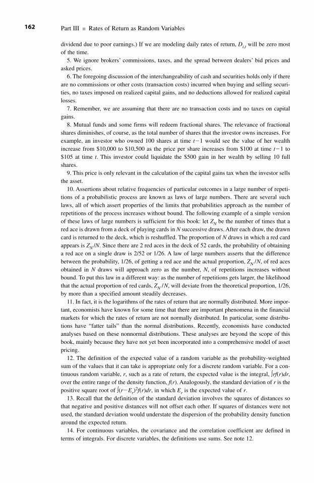
dividend due to poor earnings.) If we are modeling daily rates of return, Di,t will be zero mostof the time.

5. We ignore brokers’ commissions, taxes, and the spread between dealers’ bid prices andasked prices.

6. The foregoing discussion of the interchangeability of cash and securities holds only if thereare no commissions or other costs (transaction costs) incurred when buying and selling securi-ties, no taxes imposed on realized capital gains, and no deductions allowed for realized capitallosses.

7. Remember, we are assuming that there are no transaction costs and no taxes on capitalgains.

8. Mutual funds and some firms will redeem fractional shares. The relevance of fractionalshares diminishes, of course, as the total number of shares that the investor owns increases. Forexample, an investor who owned 100 shares at time t�1 would see the value of her wealthincrease from $10,000 to $10,500 as the price per share increases from $100 at time t�1 to$105 at time t. This investor could liquidate the $500 gain in her wealth by selling 10 fullshares.

9. This price is only relevant in the calculation of the capital gains tax when the investor sellsthe asset.

10. Assertions about relative frequencies of particular outcomes in a large number of repeti-tions of a probabilistic process are known as laws of large numbers. There are several suchlaws, all of which assert properties of the limits that probabilities approach as the number ofrepetitions of the process increases without bound. The following example of a simple versionof these laws of large numbers is sufficient for this book: let ZN be the number of times that ared ace is drawn from a deck of playing cards in N successive draws. After each draw, the drawncard is returned to the deck, which is reshuffled. The proportion of N draws in which a red cardappears is ZN /N. Since there are 2 red aces in the deck of 52 cards, the probability of obtaininga red ace on a single draw is 2/52 or 1/26. A law of large numbers asserts that the differencebetween the probability, 1/26, of getting a red ace and the actual proportion, ZN /N, of red acesobtained in N draws will approach zero as the number, N, of repetitions increases withoutbound. To put this law in a different way: as the number of repetitions gets larger, the likelihoodthat the actual proportion of red cards, ZN /N, will deviate from the theoretical proportion, 1/26,by more than a specified amount steadily decreases.

11. In fact, it is the logarithms of the rates of return that are normally distributed. More impor-tant, economists have known for some time that there are important phenomena in the financialmarkets for which the rates of return are not normally distributed. In particular, some distribu-tions have “fatter tails” than the normal distributions. Recently, economists have conductedanalyses based on these nonnormal distributions. These analyses are beyond the scope of thisbook, mainly because they have not yet been incorporated into a comprehensive model of assetpricing.

12. The definition of the expected value of a random variable as the probability-weightedsum of the values that it can take is appropriate only for a discrete random variable. For a con-tinuous random variable, r, such as a rate of return, the expected value is the integral, ∫rf(r)dr,over the entire range of the density function, f(r). Analogously, the standard deviation of r is thepositive square root of ∫(r�Er)

2f(r)dr, in which Er is the expected value of r.13. Recall that the definition of the standard deviation involves the squares of distances so

that negative and positive distances will not offset each other. If squares of distances were notused, the standard deviation would understate the dispersion of the probability density functionaround the expected return.

14. For continuous variables, the covariance and the correlation coefficient are defined interms of integrals. For discrete variables, the definitions use sums. See note 12.


15. If k is a constant, E(k)�k.16. The attractiveness of Security i also depends on the values of the correlation coefficients

between the rate of return on Security i and the rates of return on all of the other securities thatthe investor could hold. We explain this relationship in chapter 8.

17. The reader should create examples to demonstrate this.18. In fact, since the page is only two-dimensional, Figure 7.4 is a two-dimensional repre-

sentation of a three-dimensional diagram. 19. Investors who held diversified portfolios, such as mutual funds, did not lose all of their

wealth even during the bear market of 1972–74 or during the crash of 1987.20. Income could come from realizing capital gains or from dividend payments.21. That is, best fits against the criterion of minimizing the sum of the squared vertical dis-

tances between the data points and the regression line.



Part IV

Portfolio Theory and CapitalAsset Pricing Theory


8.1 Introduction

8.1.1 Definition of Portfolio Theory

A portfolio is a collection of securities. Portfolio theory is a formal analysis of therelationship between the rates of return on a portfolio of risky securities and the ratesof return on the securities contained in that portfolio. The rate of return on a portfoliois a random variable. The probability distribution that generates values for the rate ofreturn on the portfolio is a compilation of the probability distributions that generatethe rates of return on the securities contained in that portfolio. In this chapter, wedevelop an elementary version of portfolio theory. We then use that theory to explainhow a rational investor would allocate funds among risky securities to create a portfo-lio that best suits his or her preferences regarding alternative combinations of risk andexpected return.

8.1.2 The Uses of Portfolio Theory in the Economics of Financial Markets

Economists use portfolio theory to derive empirically testable models of how finan-cial markets set the prices of individual securities. The seminal application of portfo-lio theory to this question created the capital asset pricing model, which we study indetail in the next chapter. Economists derived this model by determining what theequilibrium prices of individual securities would be if all investors used the principlesof portfolio theory to construct their personal portfolios. Understanding the derivationof the capital asset pricing model from portfolio theory will contribute much to thereader’s understanding of financial economics. The same exercise will also increasethe reader’s sophistication in microeconomic theory.

By leading to the creation of asset pricing models, portfolio theory has also con-tributed in several ways to our ability to analyze the economic efficiency with whichfinancial markets allocate scarce resources. Addressing these questions of efficiencyis important for the scientific purpose of understanding how the markets work. Thisanalysis is also important as a basis for public policy toward financial markets.

Financial markets allocate scarce resources in several ways. We evaluate theperformance of these markets against the criterion of economic efficiency that wedeveloped in chapter 2. Recall that we defined economic efficiency in terms ofmutually beneficial exchanges. Most exchanges require that at least one of the parties

8 Portfolio Theory

167

in the exchange bears risk; therefore, we must have a theory of how financial marketsquantify risk and determine the reward for bearing risk if we are to assess the eco-nomic efficiency of these markets. The models of asset pricing that economists havederived from portfolio theory enable us to integrate risk into our analyses ofexchanges among investors. We next discuss briefly four ways in which financialmarkets allocate resources.

First, financial markets promote exchanges between investors who are willing toaccept lower expected rates of return in order to avoid some risk, and investors whoare willing to bear higher levels of risk in order to gain higher expected rates of return.We considered an example of this in chapter 6, where we considered the exchanges offinancial securities between Ms. Tall and Ms. Short, each of whom has differenttolerances for risk.

Second, financial markets guide the allocation of investible funds among poten-tial new projects by providing both corporations and individual investors with mecha-nisms for evaluating the levels of risk and expected rates of return on these projects.

Third, under some conditions financial markets can enable managers of firms toeliminate an asymmetry of information between themselves and potential newinvestors from whom the firm seeks additional capital to undertake new projects. Ifthe conflict created by asymmetric information is not resolved, the firm’s currentinvestors and the potential new investors will forego a mutually beneficial exchange;foregone mutually beneficial exchanges create an economically inefficient allocationof resources. In chapter 13, we show that when managers have a variety of kinds ofsecurities to offer to new investors, the managers can credibly transmit their superiorinformation to new investors by the choice of the security they offer.

The fourth way in which portfolio theory contributes to the analysis of theefficiency of financial markets involves the governance of the modern corporation.A firm’s managers act as agents of the shareholders, who own the firm’s capital.Among other things, the managers must decide how to allocate the firm’s earningsbetween investing in new projects and paying dividends. In chapter 13, we examinethe incentives that can lead managers to make choices that decrease the shareholders’wealth. Economists call this phenomenon the problem of agency. We also explain howfinancial markets can mitigate this problem by means of offering different kinds ofsecurities.

All four uses of portfolio theory have implications for public policy. Public policyshould enhance the ability of the markets to promote economic efficiency. In particu-lar, public policy should mitigate the inefficiencies created by asymmetries of infor-mation and by problems of agency. But in order to construct public policies that willpromote an efficient allocation of resources, we must understand how markets affectthe allocation of resources. To do so, we need a theory of capital asset pricing.Portfolio theory has made substantial contributions to the development and testing ofalternative theories of capital asset pricing.

8.1.3 The Plan of the Chapter

In the remainder of this chapter, we show how the expected returns, standarddeviations, and correlation coefficients of individual securities determine the set of

Part IV ■ Portfolio Theory and Capital Asset Pricing Theory168

combinations of expected return and standard deviation that an investor can choosefor a portfolio. We first consider in detail portfolios that contain only two securities.We show how the value of the correlation coefficient between these two securitiesdetermines the set of combinations of expected return and standard deviation (i.e.,risk) that the investor can obtain for his or her portfolio.

A particularly transparent use of portfolio theory occurs when two risky securitieshave perfectly correlated rates of return. In this situation, an investor can construct ariskless portfolio. Competition among investors will ensure that the rate of return onthis riskless portfolio will be equal to the rate of return on any single riskless security,such as a bank account or a government bond. In chapter 15, we use this fact to derivethe equilibrium prices of derivative securities, such as options.

The trade-off between the expected return and the standard deviation for portfo-lios that contain more than two securities is analogous to the case in which the portfo-lio contains only two securities. We summarize that analogy without the detail inwhich we analyze portfolios that contain only two risky securities.

8.2 Portfolios as Synthetic Securities

A portfolio is a synthetic security that an investor creates by purchasing a combinationof elemental securities. An elemental security is a security, such as a common stock ora bond, issued by a firm or a governmental agency.

The rate of return on a portfolio is a weighted average of the rates of return on itsconstituent securities. We know that the rate of return on a security is a random vari-able whose value is generated by a probability density function. Therefore, the rate ofreturn on the portfolio is also a random variable, and the value of the portfolio’s rate ofreturn is generated by a probability density function that is a composite of the densityfunctions for the constituent securities.

The expected return and standard deviation for the portfolio’s rate of return aredetermined by the expected returns, standard deviations, and correlation coefficientsof the securities contained in the portfolio, and by the proportions in which theinvestor allocates funds across those securities. The investor cannot choose the rate ofreturn on the portfolio because that rate of return is a random variable. By choosingthe proportions in which to allocate funds across those securities, the investor can,however, within limits, choose the expected value and the standard deviation of theprobability density function that will govern the rate of return on the portfolio. This isthe sense in which a portfolio is a synthetic security.

Here is an example. Consider two simple portfolios. Portfolio 1 contains onlySecurity A; Portfolio 2 contains Securities A, B, and C.

To construct Portfolio 1, the investor allocates 100% of the funds to Security A.To purchase Security A is to purchase the right to receive a rate of return whose valuewill be generated by Security A’s probability density function. Let σA and EA be thestandard deviation and expected return of this density function. When an investor pur-chases Security A, he or she purchases the combination of parameters (σA, EA) for thedensity function that will generate the rate of return. Since Portfolio 1 contains only

Chapter 8 ■ Portfolio Theory 169

Security A, the expected rate of return on Portfolio 1 is, obviously, EA, and the stan-dard deviation of that rate of return is σA.

Portfolio 2 contains Securities A, B, and C. The values for the rate of return onthis portfolio will be generated by a probability density function that is a composite ofthe density functions for Securities A, B, and C. Let E2 and σ2 be the expected returnand the standard deviation for Portfolio 2. By varying the proportions in which to allo-cate funds across Securities A, B, and C, the investor can choose from many alterna-tive combinations of values for the parameters E2 and σ2 that will govern the rate ofreturn on Portfolio 2. The fact that an investor can choose among several combina-tions of values for E2 and σ2 by altering the allocation of funds among individualsecurities is fundamental to understanding the economics of financial markets.

8.3 Portfolios Containing Two Risky Securities

8.3.1 Risky Securities

A risky security is a security whose rate of return will deviate randomly from itsexpected value. Therefore, the probability density function for a risky security willhave a nonzero value for its standard deviation. In portfolio theory, risky does notmean inadvisable, highly speculative, or anything else that would imply that the secu-rity is a poor investment. Rather, risky simply means not riskless.

A riskless security is one whose rate of return is guaranteed never to deviate froma known constant. The probability density function for a riskless security has a stan-dard deviation equal to zero. The graph of this density function is a single vertical lineerected at the value of the expected return.

8.3.2 The Rate of Return on the Portfolio

Let W be the amount of money that an investor uses to form a portfolio that containsonly two securities, A and B. Let XA and XB be the proportions in which the investorallocates funds to these securities. Since the portfolio contains no securities other thanA and B, then:

XA�XB�1. (8.1)

For example, if W � $1,000, and the investor chooses .7 as the value for XA and.3 as the value for XB, then he or she forms the portfolio by purchasing $700 worth ofSecurity A and $300 worth of Security B. Let the random variables rA and rB be therates of return on Securities A and B, and let the random variable rP be the rate ofreturn on the investor’s portfolio. The rate of return on the portfolio is related to therates of return on its constituent securities by:

(8.2)

The rate of return on the portfolio is a weighted average of the rates of returnon the constituent securities, with the weights being the proportions XA and XB that

� � �r r rP A A B B� �X X .


determine the structure of the portfolio. Note that the aggregate amount of funds, W,does not appear in equation (8.2). The rate of return on the portfolio is determinedsolely by the rates of return on the constituent securities and by the proportions inwhich the investor allocates funds between those securities.

Suppose that in a given month the outcomes for the rates of return on Securities Aand B are rA�.10 and rB�.18. If the investor formed a portfolio by setting XA�.7 andXB�.3, then the rate of return on the portfolio for that month would be:

(8.3)

Therefore, the value of the investor’s portfolio would have increased by 12.4% overthe month. If he or she had committed a total of W�$1,000 to the portfolio at thebeginning of the month, then the value of the portfolio at the end of the month wouldbe:

(8.4)

Had the investor committed $2,000 to the portfolio and used the same values forXA and XB, the second portfolio would have been twice the size of the first portfolio,but the two portfolios would have identical structures. Therefore, the rate of return onthe two portfolios would be equal, namely rP�.124. But the value of the larger portfo-lio at the end of the month would be $2,248, twice the ending value of the smallerportfolio.

8.3.3 Short Positions

We digress briefly to consider portfolios in which the investor takes a short position inone of the two securities. We do this because in some cases we can discover the equi-librium prices of risky securities by examining portfolios that contain these securitiesand also contain short positions in one or more related securities. In chapter 15, we usethis procedure to analyze the equilibrium prices of options.

In the numerical example in the preceding section, the investor constructed aportfolio by purchasing quantities of both Securities A and B. We know this becausethe allocative proportions XA and XB both have positive values. We say that theinvestor had long positions in both securities. If an investor is long in both securities,then the total dollar amount that she can invest in either security must be less than W,which is the aggregate value of the invested funds. If, however, the investor sells oneof the securities short, she can use the proceeds of that short sale to increase herinvestment in the other security to an amount greater than W. If the investor does takea short position in one security, the allocative proportion for that security will be neg-ative, and the proportion for the other security will be greater than 1. The sum of thetwo proportions must still be equal to 1.

Consider the following example. The investor takes a short position in Security Aby an amount equal to 40% of her total funds, W. To do this, she sets XA��.4. Since

(1 ) (1 .124)$1,000

$1,124.

� � �

�

�r WP

� � �r X r rP A A B B� �

� �

� � �

X

(.7)(.10) (.3)(.18)

.07 .054 .124.


XA�XB�1, the proportion of her total funds that she will allocate to Security B will beXB�1�XA�1�(�.4)�1.4. If W�$1,000, she will borrow $400 worth of shares ofSecurity A, sell them, and combine the proceeds of $400 with the $1,000 of her ownmoney that she has committed to the portfolio. She will then purchase $1,400 worth ofshares of Security B, so that she has a long position in that security equal to $1,400.Her long position of $1,400 in Security B exceeds by 40% the total amount of money,$1,000, that she has committed to the portfolio.

The investor’s position in Security B is long by $1,400 because that is the amountof money that she could raise if she were to liquidate her position in Security B. Sinceshe owns $1,400 worth of Security B, liquidating her position in that security wouldrequire selling $1,400 worth of that security, thus raising $1,400.

The investor’s position in Security A is equal to XAW. Since XA��.4 andW�$1,000, her position in that security is �$400, which is a short position. Her posi-tion in Security A is short by $400 because that is the amount of money that she wouldhave to pay to liquidate that position. Since she initially borrowed $400 worth ofSecurity A, she would have to spend $400 to repurchase a sufficient number of sharesof that security to extinguish her debt to owners of Security A.

In the preceding paragraph, we assumed that the prices of neither security changeafter the investor constructs the portfolio. Under this assumption, liquidating the port-folio would raise $1,400�(�$400)�$1,000, which is exactly what she invested. Ifthe prices of the two securities changed between the time that she constructed the port-folio and the time that she liquidated it, then the portfolio could, of course, be worthmore than $1,000, or less than $1,000.

8.4 The Trade-Off between the Expected Value and the Standard Deviation of the Rate of Return on a PortfolioThat Contains Two Securities

8.4.1 The Equations for the Expected Return and the StandardDeviation of the Portfolio

We shall now develop the relationship between the investor’s choice of values for XAand XB and the values of the expected return and the standard deviation on her portfolio.

The expected value of the rate of return, EP, and the standard deviation of thatrate of return, σP, on the investor’s portfolio are determined by the proportions, XAand XB, in which she allocates funds to Securities A and B, and by the five parametersthat define the probability density functions for those securities. These parameters arethe expected return and the standard deviation for Security A, the expected return and the standard deviation for Security B, and the correlation coefficient between therates of return on those securities. Specifically, EP and σP are determined by:

(8.5)

and

(8.6)s s s s s sP P A A AB A B A B B BX X X X� � � � �2 ( 2 ).2 2 2 2

E X E X EP A A B B� � ,


The term under the square root sign on the right-hand side of equation (8.6) is the vari-ance of the rate of return on the portfolio. For portfolios, it is often convenient to workwith the variance rather than the standard deviation.

8.4.2 Parameters, Decision Variables, and Independent Variables

It will be helpful to sort the many symbols that appear in the equations above intothree groups, as follows.

Parameters: EA, σA, EB, σB, ρAB.The investor has no control over the probability density functions that generate

outcomes for the rates of return on Securities A and B. These probability density func-tions are fully defined by the values of the five parameters. The values of these param-eters depend on the operational and financial decisions made by the managers ofFirms A and B, and on the relationships between the operations of these firms and theperformance of the macroeconomy in which these firms participate.

Decision variables: XA, XB.The investor chooses the values XA and XB to specify the proportions in which she

will allocate funds between Securities A and B. Since these securities are the only can-didates for the portfolio, XA�XB�1. Either XA or XB can be positive, negative, or zerodepending on whether the investor takes a long position, a short position, or no posi-tion in that security.

Dependent variables: EP, σP.The investor’s portfolio is a synthetic security that she creates by holding

Securities A and B in a certain proportion. The rate of return on the portfolio is gov-erned by a probability density function that the investor constructs by choosing valuesfor the proportions XA and XB. But the portfolio’s density function is fully defined bythe values of its expected return and its standard deviation. Equivalently, the investorchooses the combination of values for the expected return and the standard deviationon her portfolio by choosing the proportions, XA and XB, that define her portfolio. Therelationship between the investor’s decisions on XA and XB, and the consequent valuesfor EP and σP, is specified by equations (8.5) and (8.6).

8.4.3 Economic Interpretations

Here are the economic interpretations of the several terms in equations (8.5) and (8.6).From equation (8.5), we see that the expected return for the portfolio is a weightedaverage of the expected returns of the two constituent securities. The weights are theallocative proportions, XA and XB. If the investor allocates most of her funds toSecurity A, and only a small proportion to Security B, then the average rate of returnon the portfolio will be closer to the average rate of return on Security A than to theaverage rate of return on Security B. The right-hand side of equation (8.5) ensuresthis. Note from equation (8.5) that EP, the expected return on the investor’s portfolio,does not depend on the correlation coefficient, ρAB.

The portfolio’s standard deviation, σP, is defined by equation (8.6). The first andthird terms under the square root sign on the right-hand side of equation (8.6) are


analogous to the two terms that define EP in equation (8.5). When calculating EP, weput on the expected return for each constituent security a weight that is equal to the proportion of the funds allocated to that security. When calculating the standarddeviation for the portfolio, we square the weighted standard deviations of Securities Aand B.

The standard deviation for the portfolio is also affected by the interactionbetween the rates of return on Securities A and B. The effect of this interaction ismeasured in equation (8.6) by the middle term, which contains the correlation coeffi-cient, ρAB. The reason is easy to understand.

The standard deviation for any random variable measures the dispersion of valuesthat the random variable can take above and below its expected value. More precisely,the standard deviation is a probability-weighted measure of dispersion around thatexpected value. Therefore, the standard deviation for the portfolio will increase if therates of return on Securities A and B interact in a way that increases the probabilitythat the rate of return on the portfolio, rP, will take values far above, and far below, itsexpected value, EP. Similarly, if the interaction between Securities A and B decreasesthe probability that rP will take values from EP, then including those two securities inthe portfolio will decrease the standard deviation of the rate of return on the portfolio.

The value and the sign of the correlation coefficient between the rates of return onSecurities A and B is a measure of the effect of those securities on the probabilitiesthat the rate of return on the portfolio will take values far above and far below EP.Here is the reason.

Suppose that the value of the correlation coefficient is large and positive. Forexample, suppose that ρAB�.9. Then in any given month, the rates of return onSecurities A and B are highly likely to be on the same sides of their respectiveexpected values. Moreover, the number of Security A’s standard deviations by whichrA is displaced from EA is highly likely to be equal to the number of Security B’s stan-dard deviations by which rB is displaced from EB. That is, the rates of return for thetwo securities will lie the same standardized distance away from their respectiveexpected values.

For example, suppose that in a given month the rate of return for Security A liesabove EA by a distance of 2.5σA. Then the fact that ρAB�.9 means that there is a highprobability that the rate of return for Security B for that month will lie above EB by adistance of 2.5σB. If ρAB were equal to �1, which is the maximal value that a correla-tion coefficient can take, then the probability would be 1 (100%) that rB will take thevalue of EB�2.5σB whenever rA takes the value EA�2.5σA.

Similarly, suppose that in a given month rA takes a value below EA. If ρAB�.9,there is a high probability that the number of Security B’s standard deviations bywhich rB lies below EB will be equal to the number of Security A’s standard deviationsby which rA lies below EA.

Finally, if the correlation coefficient, ρAB, is large and negative, there is a highprobability that in any given month the rates of return on Securities A and B will lie onopposite sides of their respective expected rates of return at distances equal to thesame number of their respective standard deviations.

We can now see the effect of the value of ρAB on the size of the standard deviationof the rate of return on a portfolio that contains both Securities A and B. The standard


deviation for the portfolio, σP, measures the dispersion of values for the rate of returnon the portfolio above and below the expected rate of return on the portfolio, EP. Fromequation (8.5), we know that the value of EP is a weighted average of the expectedrates of return, EA and EB, on the constituent securities. In any given month, the rate ofreturn on the portfolio is a weighted average of the rates of return on Securities A andB for that month. If the rates of return on both securities are simultaneously above (orbelow) their respective expected rates of return, then the two securities will reinforceeach other in moving the rate of return on the portfolio above (or below) its expectedrate of return. In particular, if the rates of return on Securities A and B are simultane-ously far above (or far below) their expected rates of return, then the rate of return onthe portfolio will be far above (or far below) its expected rate of return. The higher thevalue of the correlation coefficient, ρAB, the higher the probability that the rates ofreturn on Securities A and B in a given month will lie on the same sides of theirrespective expected rates of return by the same number of their respective standarddeviations. Consequently, the higher the value of ρAB, the higher the probability thatthe interaction between Securities A and B will amplify the dispersion of values forthe rate of return on the portfolio. Therefore, the larger the value for ρAB, the larger thevalue for σP.

Using analogous reasoning, we conclude that if the value of the correlation coef-ficient is large and negative, the probability is high that the inclusion of Securities Aand B in the portfolio will have offsetting effects on the rate of return on the portfolio.Therefore, the smaller (more negative) the value for ρAB, the smaller the value for σP.

8.4.4 The Locus of Combinations of Expected Returns and StandardDeviations for Portfolios

We will now use a graph to increase our understanding of how an investor can alter thecombination of expected return and standard deviation on a portfolio. Each point infigure 8.1 represents a specific combination of expected return and standard deviationon a portfolio. Expected return is measured in the vertical dimension, and standarddeviation is measured in the horizontal dimension. We want to draw a locus of thosecombinations of expected return and standard deviation that the investor can con-struct. From our discussions of equations (8.5) and (8.6), we know that the combina-tions of expected return and standard deviation that the investor can choose for aportfolio are determined by the values of the five parameters EA, σA, EB, σB, and ρAB.To construct an example of a locus, suppose that the values of the first four parametersare EA�.20, σA�.06, EB�.10, and σB�.02. We will leave the value of the correlationcoefficient unspecified for the moment.

The investor constructs a portfolio by choosing an allocation of funds betweenSecurities A and B. One of her choices is to allocate 100% of her funds to Security A,and none to Security B. To do this, she would set XA�1 and XB�0. If she holds onlySecurity A in her portfolio, then the rate of return on her portfolio will be simply therate of return on Security A; the rate of return on Security B will be irrelevant. Thenthe expected return, EP, and the standard deviation, σP, on the investor’s portfolio willbe equal to the expected return and the standard deviation on the only security in thatportfolio. That is, EP�EA and σP�σA.


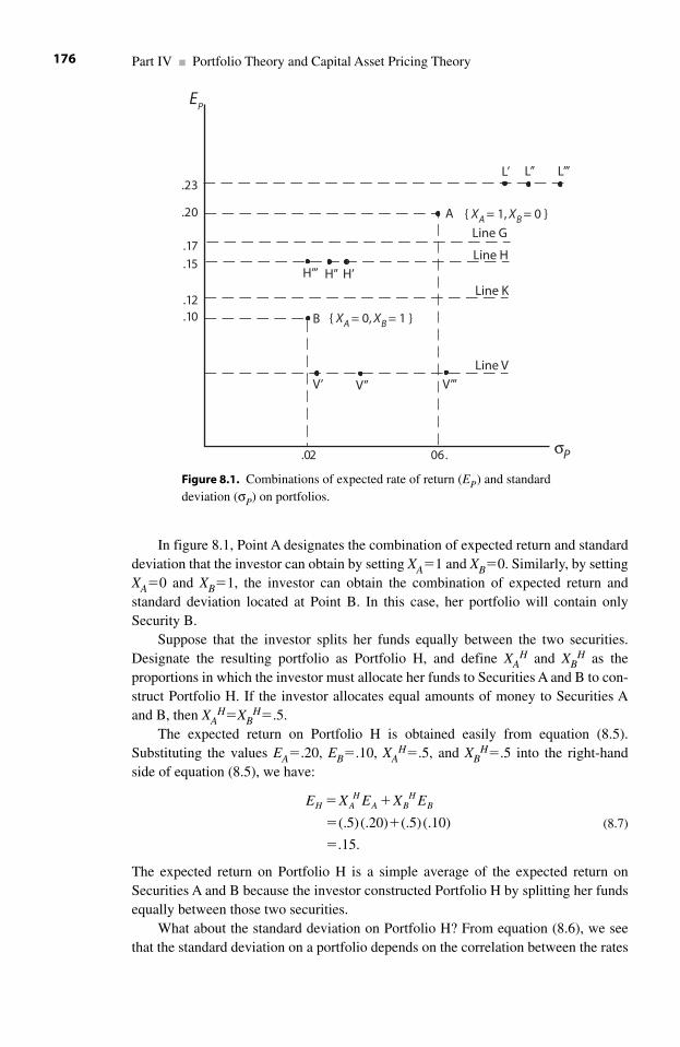
In figure 8.1, Point A designates the combination of expected return and standarddeviation that the investor can obtain by setting XA�1 and XB�0. Similarly, by settingXA�0 and XB�1, the investor can obtain the combination of expected return andstandard deviation located at Point B. In this case, her portfolio will contain onlySecurity B.

Suppose that the investor splits her funds equally between the two securities.Designate the resulting portfolio as Portfolio H, and define XA

H and XBH as the

proportions in which the investor must allocate her funds to Securities A and B to con-struct Portfolio H. If the investor allocates equal amounts of money to Securities Aand B, then XA

H�XBH�.5.

The expected return on Portfolio H is obtained easily from equation (8.5).Substituting the values EA�.20, EB�.10, XA

H�.5, and XBH�.5 into the right-hand

side of equation (8.5), we have:

(8.7)

The expected return on Portfolio H is a simple average of the expected return onSecurities A and B because the investor constructed Portfolio H by splitting her fundsequally between those two securities.

What about the standard deviation on Portfolio H? From equation (8.6), we seethat the standard deviation on a portfolio depends on the correlation between the rates

E X E X EH AH

A BH

B� �

� �

�

(.5)(.20) (.5)(.10)

.15.


Figure 8.1. Combinations of expected rate of return (EP) and standarddeviation (σP) on portfolios.

.10

.12

.15

.17

.20

.23

.02 .06 σP

EP

Line G

Line H

Line K

Line V

{ XA = 0, XB = 1 }

{ XA = 1, XB = 0 }

B

V’ V’’ V’’’

L’L’ ’ L’’’

H’H’’H’’’

A

of return on Securities A and B through the middle term, 2ρABσAσBXAHXB

H. But thecorrelation coefficient, ρAB, does not appear in equation (8.5), which determines thevalue for EH. Therefore, EH will be equal to .15 regardless of the value of ρAB. Weconclude that the combination of expected return and standard deviation in PortfolioH will lie along Line H in figure 8.1. The vertical intercept of Line H is at EP�.15.

We next consider two other portfolios, which we will call Portfolio G andPortfolio K. To construct Portfolio G, the investor allocates 70% of her funds toSecurity A, and the balance to Security B. Define XA

G and XBG as the allocative pro-

portions that define Portfolio G. Then XAG�.7 and XB

G�.3. Using equation (8.5), theexpected return on Portfolio G will be:

(8.8)

As in the case of Portfolio H, the correlation coefficient between the rates of return onSecurities A and B will affect the standard deviation on Portfolio G but not theexpected return on that portfolio. Therefore, in figure 8.1 the combination of expectedreturn and standard deviation for Portfolio G will lie on the horizontal line labeledLine G, whose vertical intercept is at EP�.17.

Finally, let Portfolio K be defined by the allocative proportions XAK�.2 and

XBK�.8. The combination of expected return and standard deviation for Portfolio K

will lie on Line K in figure 8.1. The vertical intercept of this line is EK�.12, whichresult we obtain by using equation (8.5) and using the values XA

K�.2 and XBK�.8 for

the allocative proportions.

8.4.5 The Effect of the Correlation Coefficient ρAB on the Expected Returnand the Standard Deviation of the Portfolio

We know from equation (8.5) that the value of the correlation coefficient between therates of return on Securities A and B has no effect on the expected return of PortfolioH (or any portfolio). The correlation coefficient does, however, affect the standarddeviation for Portfolio H through the middle term in equation (8.6); this term is2ρABσAσBXA

HXBH once we substitute XA

H and XBH for XA and XB.

Portfolio H contains positive investments in both Securities A and B because bothXA

H and XBH are positive. The two standard deviations, σA and σB, are also positive.

Therefore, the value of the term 2ρABσAσBXAHXB

H varies directly with the value of the correlation coefficient, ρAB. Consequently, for any fixed allocation of fundsbetween Securities A and B, the smaller the value of the correlation coefficientbetween the rates of return on Securities A and B, the smaller the standard deviation ofthe portfolio.

Consider three alternative values for the correlation coefficient, as follows:

(8.9)

Each of these three alternative values for ρAB generates a value for the standard devi-ation on Portfolio H. Let σH ′ be the standard deviation for Portfolio H for the case in

ρ ρ ρ′ ′′ ′′′AB AB AB� � � �.8; .1; .6.

E X E X EG AG

A BG

B� �

� �

�

(.7)(.20) (.3)(.10)

.17.


which ρAB�ρAB′�.8. Similarly, let σH″ and σH″′ be the standard deviations forPortfolio H when ρAB takes the values ρAB�ρAB″�.1, or ρAB�ρAB″′��.6. Since ρABaffects the standard deviation on Portfolio H only through the term 2ρABσAσBXA

HXBH

in equation (8.6), and since σA, σB, XAH, and XB

H are all positive numbers, we con-clude that the three alternative values for the standard deviation on Portfolio H, corre-sponding to the three alternative values for the correlation coefficient, satisfy theranking:

(8.10)

In figure 8.1, three points are plotted on the horizontal line labeled Line H. Eachpoint designates a combination of expected return and standard deviation for PortfolioH that corresponds to one of the three alternative values for ρAB. Point H′ correspondsto the case in which ρAB�ρAB′�.8. Similarly, Points H″ and H″′ correspond to thecases in which ρAB�ρAB″�.1, or ρAB�ρAB″′��.6. The points H′, H″, and H″′ lie atthe same height because the value of ρAB has no effect on the expected return forPortfolio H. From equation (8.6), we know that the standard deviation on Portfolio Hdecreases as the value of ρAB decreases. Therefore, as ρAB decreases from .8 to .1 to�.6, the combination of expected return and standard deviation for Portfolio H moveshorizontally leftward along Line H from Point H′ to Point H″ to Point H″′.

Our analysis of the effect of the value of ρAB on the combination of expectedreturn and standard deviation for Portfolio H also holds for Portfolios G and K. As thevalue of ρAB decreases, the points in figure 8.1 that designate the combinations ofexpected return and standard deviation for Portfolios G and K move horizontally left-ward along the lines labeled Line G and Line K.

Thus far we have considered portfolios in which the investor either holds positivequantities of both Securities A and B, or places 100% of the funds in one of thosesecurities and holds none of the other security. The combinations of expected returnand standard deviation that characterize these portfolios lie on a line in figure 8.1 thatpasses from Point A to Point B. We know that the locus must pass through these pointsbecause two of the portfolios that the investor can construct consist of placing 100%of the funds in one security and none of the funds in the other security.

The degree of curvature of the locus increases as the value of the correlation coef-ficient between the rates of return on Securities A and B decreases from �1 to �1. Insection 8.6, we show that when ρAB takes its maximal value, �1, the combinations ofexpected return and standard deviation on portfolios that contain only Securities A andB all lie on the straight line that connects Points A and B. That is, when ρAB��1, thelocus of combinations of expected return and standard deviation has no curvature atall. As ρAB decreases, the locus becomes more sharply curved to the left. If ρAB takesits minimal value, �1, then the locus becomes two straight lines that intersect on thevertical axis at a point between EB�.10 and EA�.20. One of these lines slopes upwardfrom this point on the vertical axis to Point A. The other line slopes downward fromthis point to Point B.

We now consider the combinations of expected return and standard deviation thatthe investor can choose for a portfolio by taking a short position in one of the twosecurities.

H H H′ ″ ″′> > .


Suppose that the investor constructs Portfolio L by taking a short position inSecurity B equal to 30% of her initial funds. To do this, she sets the value ofXB

L��.3. Since Securities A and B are the only securities in her portfolio, we musthave XA

L�XBL�1. This condition, and her choice that XB

L��3, means thatXA

L�1�XB�1�(�.3)�1.3. For example, suppose that the investor’s initial fundswere $100. She would then purchase $130 worth of Security A, financing this pur-chase by using $100 of her own funds augmented by the $30 that she raises by sellingborrowed shares of Portfolio B. The expected return on Portfolio L will be:

(8.11)

Notice that the expected return on Portfolio L lies outside the interval between EB�.10and EA�.20. Since the correlation coefficient ρAB has no effect on the expected returnon a portfolio, the combination of expected return and standard deviation for PortfolioL will lie somewhere on Line L in figure 8.1. The height of this line is .23.

Now consider the effect of ρAB on the standard deviation for Portfolio L.Recalling our earlier work, the correlation coefficient will affect σ L through the mid-dle term of:

(8.12)

In Portfolio L, the investor holds Security A long and Security B short. Therefore,XA

LXBL is negative. In our numerical example, XA

LXBL�(1.3)(�.3)��3.9. Since the

product σAσB is positive, the term 2ρABσAσBXALXB

L will increase as the value of ρABdecreases from �1 to �1. In figure 8.1, let the points L′, L″, and L″′ designate thethree combinations of expected return and standard deviation for Portfolio L that cor-respond to the alternative values for ρAB, namely ρAB′�.8, ρAB″�.1, and ρAB″′��.6.Then the corresponding three values of the standard deviation for Portfolio L must beordered as follows:

(8.13)

so that in figure 8.1, Point L′ lies farthest to the left on Line L, and Point L″′ liesfarthest to the right on that line.

Next consider Portfolio V, in which the investor holds a short position in SecurityA. For Portfolio V, XA

V0 and XBV�1. Following an argument analogous to the one

we used for Portfolio L, we can conclude that the expected return on Portfolio V isless than the expected return on Security B. Therefore, the combination of expectedreturn and standard deviation for Portfolio V lies somewhere on the horizontal linelabeled Line V in figure 8.1. Further, since XA

V0 and XBV�1, the product XA

VXBV is

negative. Therefore, as is the case with Portfolio L, the standard deviation of PortfolioV increases as the value of ρAB decreases from �1 to �1. The points V′, V″, and V″′on Line V in figure 8.1 designate the three combinations of expected return and stan-dard deviation for Portfolio V that correspond to the three alternative values for ρAB.

We can summarize our analysis thus far by considering the three loci in figure8.2. Each locus is a set of alternative combinations of expected return and standard

′ ′′ ′′′> >L L L ,

� � � � L AL

A AB A B AL

BL

BL

BX X X X[( ) 2 ( ) ].2 2 2 2

E X E X EL AL

A BL

B� �

� � �

�

(1.3)(.20) ( .3)(.10)

.23.


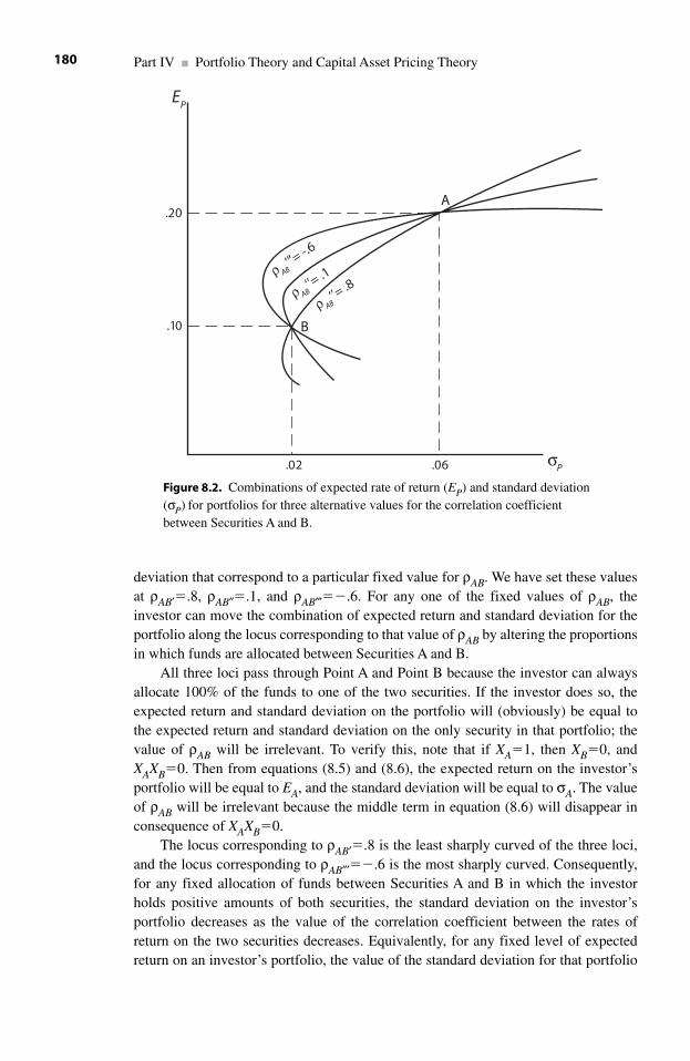
deviation that correspond to a particular fixed value for ρAB. We have set these valuesat ρAB′�.8, ρAB″�.1, and ρAB″′��.6. For any one of the fixed values of ρAB, theinvestor can move the combination of expected return and standard deviation for theportfolio along the locus corresponding to that value of ρAB by altering the proportionsin which funds are allocated between Securities A and B.

All three loci pass through Point A and Point B because the investor can alwaysallocate 100% of the funds to one of the two securities. If the investor does so, theexpected return and standard deviation on the portfolio will (obviously) be equal tothe expected return and standard deviation on the only security in that portfolio; thevalue of ρAB will be irrelevant. To verify this, note that if XA�1, then XB�0, andXAXB�0. Then from equations (8.5) and (8.6), the expected return on the investor’sportfolio will be equal to EA, and the standard deviation will be equal to σA. The valueof ρAB will be irrelevant because the middle term in equation (8.6) will disappear inconsequence of XAXB�0.

The locus corresponding to ρAB′�.8 is the least sharply curved of the three loci,and the locus corresponding to ρAB″′��.6 is the most sharply curved. Consequently,for any fixed allocation of funds between Securities A and B in which the investorholds positive amounts of both securities, the standard deviation on the investor’sportfolio decreases as the value of the correlation coefficient between the rates ofreturn on the two securities decreases. Equivalently, for any fixed level of expectedreturn on an investor’s portfolio, the value of the standard deviation for that portfolio


Figure 8.2. Combinations of expected rate of return (EP) and standard deviation(σP) for portfolios for three alternative values for the correlation coefficientbetween Securities A and B.

.02

.10

.20

.06 σP

EP

B

A

ρ AB‘’’=

-.6

ρ AB‘’=

.1

ρ AB‘’=

.8

decreases as the correlation between the two securities decreases. Using our work insection 8.4.3, we will show why this is true.

If the correlation coefficient is large and positive, there is a high probability thatin any given month the values for the rates of return on Securities A and B, rA and rB,will lie on the same sides of their expected values. Moreover, whenever the rate ofreturn for either of the securities takes a value that is far from its expected return inone direction, there is a high probability that the rate of return on the other securitywill take a value that is far from its expected return and in the same direction. If theinvestor holds positive amounts of both Securities A and B in the portfolio, and if thecorrelation between these securities is large and positive, then the random values ofthe two rates of return are likely to reinforce each other in their effects on the volatil-ity of the rate of return on the portfolio.

If Securities A and B are mutually reinforcing in their effects on the volatility of therate of return of the portfolio, then the standard deviation of the portfolio will be rela-tively large. Alternatively, if the correlation coefficient is large and negative, then thereis a high probability that in any given month the values for rA and rB will lie on oppositesides of their expected values. Moreover, whenever the rate of return for either securitydeviates far from its expected return in one direction, the rate of return for the othersecurity will be highly likely to deviate far from its expected return in the opposite direc-tion. Therefore, if the investor holds positive amounts of both securities, and if the cor-relation coefficient is large and negative, the random variations in the two rates of returnare likely to offset each other in their effects on the standard deviation of the portfolio.

Imagine two inexperienced paddlers sitting in a canoe. Suppose that each paddleris inclined to shift his weight unpredictably to one side or the other. If the two paddlersshift their weights with a large and positive correlation, then the random shifts of thetwo paddlers are likely to reduce the stability of the canoe (perhaps leading to a cap-sizing). But if the two paddlers shift their weights with a large and negative correla-tion, the random shifts are likely to increase the stability of the canoe.

The preceding analysis applies to portfolios in which the investor holds positivequantities of both securities. For all of these portfolios, the expected returns lie withinthe interval bounded by EA and EB. If the investor has a short position in one security(and thus a long position in the other), then the product XAXB will be negative.Consequently, the expected return on the portfolio will lie either above EA or belowEB. Moreover, for these portfolios, the middle term for the standard deviation in equa-tion (8.12), 2ρABσAσBXAXB, will vary inversely with the value of the correlation coef-ficient. Therefore, for any fixed allocation of funds between Securities A and B inwhich the investor holds a short position in one of those securities, an increase in thevalue of ρAB will cause the standard deviation on the portfolio to increase.

The effect of ρAB on the combinations of expected return and standard deviationthat the investor can construct by using Securities A and B is summarized by the threeloci in figure 8.2. For reasons previously discussed, all three loci pass through PointsA and B. For portfolios in which the investor holds fixed positive amounts of bothsecurities, a decrease in the value of ρAB will reduce the standard deviation on theportfolio, thus shifting the locus leftward. For portfolios in which the investor holds afixed short position in one of the securities (and thus a fixed long position in the othersecurity), a decrease in the value of ρAB will increase the standard deviation on the


portfolio, thus shifting the locus rightward. In neither case will a change in ρAB affectthe expected return on the portfolio. Since all loci must pass through Points A and B, adecrease in the value of ρAB will cause a locus to become more sharply curved.

8.5 A Simple Numerical Example to Show the Effect of �AB on the Trade-Off between Expected Return and Standard Deviation

In section 7.7 of chapter 7, we calculated the expected values, the standard deviations,and the correlation coefficient for a simple numerical example of a joint probabilitydistribution of the rates of return on Securities A and B. The values of those parame-ters are shown in table 8.1. In chapter 7, we explained that the correlation coefficientbetween the rates of return on two securities governs the amount by which the condi-tional probability density function for one security shifts in response to a specific out-come for the rate of return on the other security. Let the rate of return on Security B formonth t take a value that is displaced from its expected return by a distance equal to �^

times the standard deviation for Security B. The value of �^ can be positive, negative,or zero. Then, using the values of the parameters of the joint distribution of SecuritiesA and B, the conditional expected return and standard deviation for Security A formonth t are:

In words, the unconditional probability density function for Security A is centeredon the value .20; the standard deviation of this density function is .1897. We havedrawn this density function in figure 8.3. But the value drawn for the rate of return on Security A in a given month is connected to the rate of return drawn for Security B in that month through the correlation coefficient between Securities A and B.

2 2

2 2

ˆ ˆ( )

ˆ.20 (.706) (.1897)

ˆ.20 .1339 ,

ˆ( ) [1 ( ) ]

(.1897) [1 (.706) ]

.018049

.1343.

A B B B A AB A

A B B B A AB

E r r E E

r r E

� ��

� � �

� � �

� ��

� �

�

�

⏐ σ ρ σ

σ ⏐ σ σ ρ

� �

� �


(8.14)

Table 8.1Values of the Parameters for Securities A and B for theJoint Probability Distribution in Table 7.1

EA�.20; σA�.1897

EB�.20; σB�.0224

ρAB�.706

and

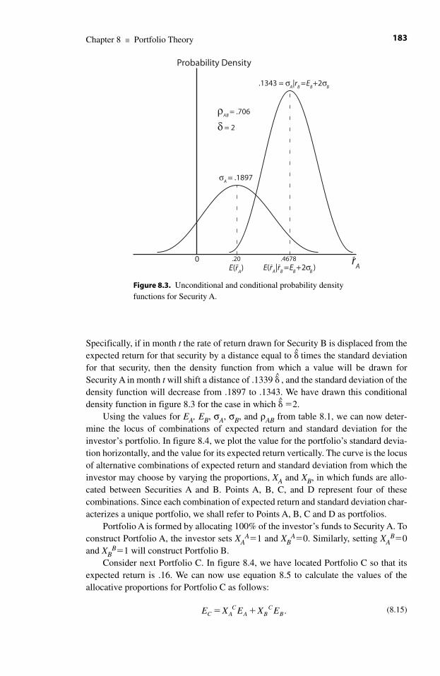
Specifically, if in month t the rate of return drawn for Security B is displaced from theexpected return for that security by a distance equal to �^ times the standard deviationfor that security, then the density function from which a value will be drawn forSecurity A in month t will shift a distance of .1339 �^ , and the standard deviation of thedensity function will decrease from .1897 to .1343. We have drawn this conditionaldensity function in figure 8.3 for the case in which �^ �2.

Using the values for EA, EB, σA, σB, and ρAB from table 8.1, we can now deter-mine the locus of combinations of expected return and standard deviation for theinvestor’s portfolio. In figure 8.4, we plot the value for the portfolio’s standard devia-tion horizontally, and the value for its expected return vertically. The curve is the locusof alternative combinations of expected return and standard deviation from which theinvestor may choose by varying the proportions, XA and XB, in which funds are allo-cated between Securities A and B. Points A, B, C, and D represent four of thesecombinations. Since each combination of expected return and standard deviation char-acterizes a unique portfolio, we shall refer to Points A, B, C and D as portfolios.

Portfolio A is formed by allocating 100% of the investor’s funds to Security A. Toconstruct Portfolio A, the investor sets XA

A�1 and XBA�0. Similarly, setting XA

B�0and XB

B�1 will construct Portfolio B.Consider next Portfolio C. In figure 8.4, we have located Portfolio C so that its

expected return is .16. We can now use equation 8.5 to calculate the values of theallocative proportions for Portfolio C as follows:

(8.15)E X E X EC AC

A BC

B� � .


Figure 8.3. Unconditional and conditional probability densityfunctions for Security A.

rA

Probability Density

E(rA) E(r

A|r

B=E

B+2σ

B)

.1343 = σA|r

B=E

B+2σ

B

0 .20 .4678

ρAB

= .706

δ = 2

σA

= .1897

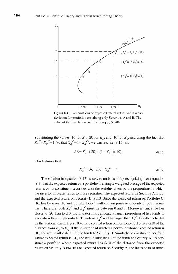
Substituting the values .16 for EC, .20 for EA, and .10 for EB, and using the fact thatXA

C�XBC�1 (so that XB

C�1�XAC), we can rewrite (8.15) as:

(8.16)

which shows that:

(8.17)

The solution in equation (8.17) is easy to understand by recognizing from equation(8.5) that the expected return on a portfolio is a simple weighted average of the expectedreturns on its constituent securities with the weights given by the proportions in whichthe investor allocates funds to those securities. The expected return on Security A is .20,and the expected return on Security B is .10. Since the expected return on Portfolio C,.16, lies between .10 and .20, Portfolio C will contain positive amounts of both securi-ties. Therefore, both XA

C and XBC must lie between 0 and 1. Moreover, since .16 lies

closer to .20 than to .10, the investor must allocate a larger proportion of her funds toSecurity A than to Security B. Therefore XA

C will be larger than XBC. Finally, note that

on the vertical axis in figure 8.4, the expected return on Portfolio C, .16, lies 6/10 of thedistance from EB to EA. If the investor had wanted a portfolio whose expected return is.10, she would allocate all of the funds to Security B. Similarly, to construct a portfoliowhose expected return is .20, she would allocate all of the funds to Security A. To con-struct a portfolio whose expected return lies 6/10 of the distance from the expectedreturn on Security B toward the expected return on Security A, the investor must move

X XAC

BC� �.6, and .4.

.16 (.20) (1 )(.10),� � �X XAC

AC


Figure 8.4. Combinations of expected rate of return and standarddeviation for portfolios containing only Securities A and B. Thevalue of the correlation coefficient is ρAB 5 .706.

.02240 .1199 .1897

.10

.16

.20

σP

EP

B

C

D

A

ρA B= .706

{ XAA = 1, X B

A = 0 }

{ XAC = .6, X B

C = .4 }

{ XAB = 0,X B

B = 1 }

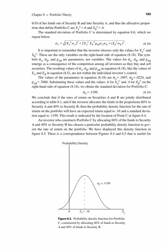
6/10 of her funds out of Security B and into Security A, and thus the allocative propor-tions that define Portfolio C are XA

C�.6 and XBC�.4.

The standard deviation of Portfolio C is determined by equation 8.6, which werepeat below.

(8.18)

It is important to remember that the investor chooses only the values for XAC and

XBC. These are the only variables on the right-hand side of equation (8.18). The sym-

bols σA, σB, and ρAB are parameters, not variables. The values for σA, σB, and ρABemerge as a consequence of the competition among all investors as they buy and sellsecurities. The resulting values of σA, σB, and ρAB in equation (8.18), like the values ofEA and EB in equation (8.5), are not within the individual investor’s control.

The values of the parameters in equation (8.18) are σA�.1897, σB�.0224, andρAB�.7060. Substituting these values and the values .6 for XA

C and .4 for XBC on the

right-hand side of equation (8.18), we obtain the standard deviation for Portfolio C:

σC�.1199. (8.19)

We conclude that if the rates of return on Securities A and B are jointly distributedaccording to table 8.1, and if the investor allocates the funds in the proportions 60% toSecurity A and 40% to Security B, then the probability density function for the rate ofreturn on the portfolio will have an expected return equal to .16 and a standard devia-tion equal to .1199. This result is indicated by the location of Point C in figure 8.4.

An investor who constructs Portfolio C by allocating 60% of the funds to SecurityA and 40% to Security B has chosen a particular probability density function to gov-ern the rate of return on the portfolio. We have displayed this density function infigure 8.5. There is a correspondence between Figures 8.4 and 8.5 that is useful for

� � � � C AC

A AC

BC

AB A B BC

BX X X X[ ] 2 ( ) .2 2


Figure 8.5. Probability density function for PortfolioC, constructed by allocating 60% of funds to SecurityA and 40% of funds to Security B.

rC

Probability Density

E C = .160

σC = .1199

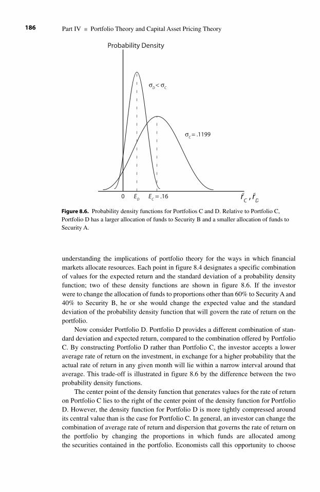
understanding the implications of portfolio theory for the ways in which financialmarkets allocate resources. Each point in figure 8.4 designates a specific combinationof values for the expected return and the standard deviation of a probability densityfunction; two of these density functions are shown in figure 8.6. If the investor were to change the allocation of funds to proportions other than 60% to Security A and40% to Security B, he or she would change the expected value and the standard deviation of the probability density function that will govern the rate of return on theportfolio.

Now consider Portfolio D. Portfolio D provides a different combination of stan-dard deviation and expected return, compared to the combination offered by PortfolioC. By constructing Portfolio D rather than Portfolio C, the investor accepts a loweraverage rate of return on the investment, in exchange for a higher probability that theactual rate of return in any given month will lie within a narrow interval around thataverage. This trade-off is illustrated in figure 8.6 by the difference between the twoprobability density functions.

The center point of the density function that generates values for the rate of returnon Portfolio C lies to the right of the center point of the density function for PortfolioD. However, the density function for Portfolio D is more tightly compressed aroundits central value than is the case for Portfolio C. In general, an investor can change thecombination of average rate of return and dispersion that governs the rate of return onthe portfolio by changing the proportions in which funds are allocated amongthe securities contained in the portfolio. Economists call this opportunity to choose


Figure 8.6. Probability density functions for Portfolios C and D. Relative to Portfolio C,Portfolio D has a larger allocation of funds to Security B and a smaller allocation of funds toSecurity A.

rC

, rD

Probability Density

EC = .16E

D0

σC

= .1199

σD

< σC

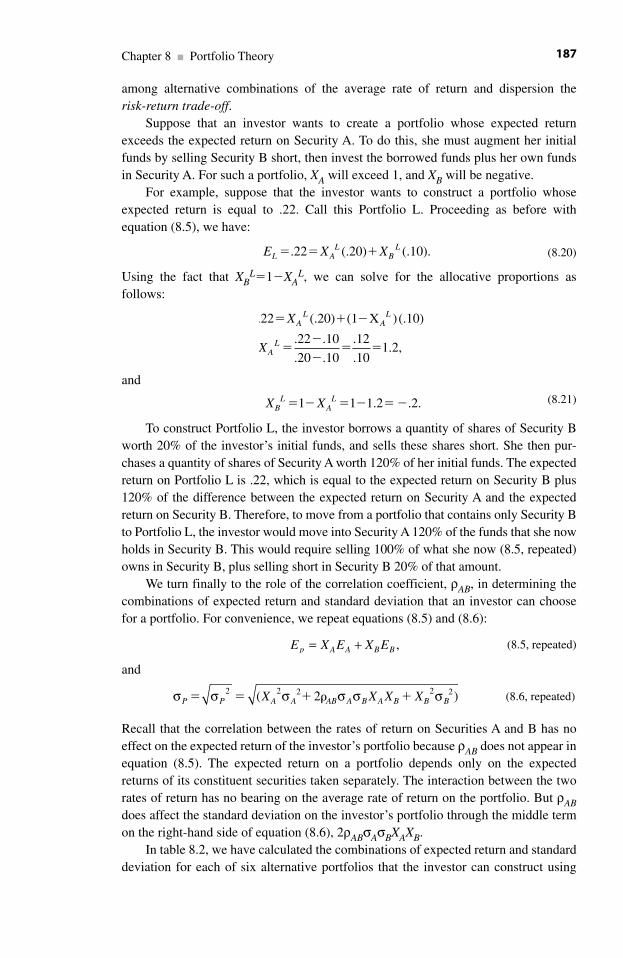
among alternative combinations of the average rate of return and dispersion the risk-return trade-off.

Suppose that an investor wants to create a portfolio whose expected returnexceeds the expected return on Security A. To do this, she must augment her initialfunds by selling Security B short, then invest the borrowed funds plus her own fundsin Security A. For such a portfolio, XA will exceed 1, and XB will be negative.

For example, suppose that the investor wants to construct a portfolio whoseexpected return is equal to .22. Call this Portfolio L. Proceeding as before withequation (8.5), we have:

(8.20)

Using the fact that XBL�1�XA

L, we can solve for the allocative proportions asfollows:

and

(8.21)

To construct Portfolio L, the investor borrows a quantity of shares of Security Bworth 20% of the investor’s initial funds, and sells these shares short. She then pur-chases a quantity of shares of Security A worth 120% of her initial funds. The expectedreturn on Portfolio L is .22, which is equal to the expected return on Security B plus120% of the difference between the expected return on Security A and the expectedreturn on Security B. Therefore, to move from a portfolio that contains only Security Bto Portfolio L, the investor would move into Security A 120% of the funds that she nowholds in Security B. This would require selling 100% of what she now (8.5, repeated)owns in Security B, plus selling short in Security B 20% of that amount.

We turn finally to the role of the correlation coefficient, ρAB, in determining thecombinations of expected return and standard deviation that an investor can choosefor a portfolio. For convenience, we repeat equations (8.5) and (8.6):

(8.5, repeated)

and

(8.6, repeated)

Recall that the correlation between the rates of return on Securities A and B has noeffect on the expected return of the investor’s portfolio because ρAB does not appear inequation (8.5). The expected return on a portfolio depends only on the expectedreturns of its constituent securities taken separately. The interaction between the tworates of return has no bearing on the average rate of return on the portfolio. But ρABdoes affect the standard deviation on the investor’s portfolio through the middle termon the right-hand side of equation (8.6), 2ρABσAσBXAXB.

In table 8.2, we have calculated the combinations of expected return and standarddeviation for each of six alternative portfolios that the investor can construct using

s s s s s sP P A A AB A B A B B BX X X X� � � � �2 ( 2 )2 2 2 2

E X E X Ep A A B B= + ,

X XBL

AL� � � � � �1 1 1.2 .2.

.22 (.20) (1 X )(.10)

.22 .10

.20 .10

.12

.101.2,

� � �

��

��

X

X

AL

AL

AL

E X XL AL

BL� � �.22 (.20) (.10).


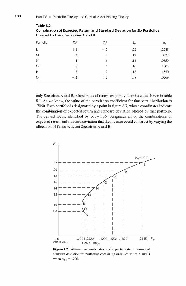
only Securities A and B, whose rates of return are jointly distributed as shown in table8.1. As we know, the value of the correlation coefficient for that joint distribution is.7060. Each portfolio is designated by a point in figure 8.7, whose coordinates indicatethe combination of expected return and standard deviation offered by that portfolio.The curved locus, identified by ρAB�.706, designates all of the combinations ofexpected return and standard deviation that the investor could construct by varying theallocation of funds between Securities A and B.


Table 8.2Combination of Expected Return and Standard Deviation for Six PortfoliosCreated by Using Securities A and B

Portfolio XAp XB

p EP σp

L 1.2 �.2 .22 .2245

M .2 .8 .12 .0522

N .4 .6 .14 .0859

O .6 .4 .16 .1203

P .8 .2 .18 .1550

Q �.2 1.2 .08 .0269

Figure 8.7. Alternative combinations of expected rate of return andstandard deviation for portfolios containing only Securities A and Bwhen ρAB � .706.

.0224.0269

.05220 .1203 .1550 .2245.0859

.1897

.10

.12

.14

.18

.22

.08

.16

.20

σP

EP

B

Q

M

N

O

P

L

A

ρAB

= .706

(Not to Scale)

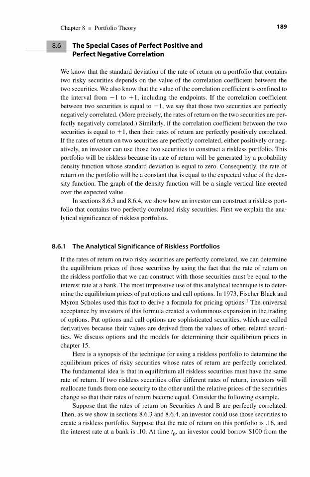
8.6 The Special Cases of Perfect Positive and Perfect Negative Correlation

We know that the standard deviation of the rate of return on a portfolio that containstwo risky securities depends on the value of the correlation coefficient between thetwo securities. We also know that the value of the correlation coefficient is confined tothe interval from �1 to �1, including the endpoints. If the correlation coefficientbetween two securities is equal to �1, we say that those two securities are perfectlynegatively correlated. (More precisely, the rates of return on the two securities are per-fectly negatively correlated.) Similarly, if the correlation coefficient between the twosecurities is equal to �1, then their rates of return are perfectly positively correlated.If the rates of return on two securities are perfectly correlated, either positively or neg-atively, an investor can use those two securities to construct a riskless portfolio. Thisportfolio will be riskless because its rate of return will be generated by a probabilitydensity function whose standard deviation is equal to zero. Consequently, the rate ofreturn on the portfolio will be a constant that is equal to the expected value of the den-sity function. The graph of the density function will be a single vertical line erectedover the expected value.

In sections 8.6.3 and 8.6.4, we show how an investor can construct a riskless port-folio that contains two perfectly correlated risky securities. First we explain the ana-lytical significance of riskless portfolios.

8.6.1 The Analytical Significance of Riskless Portfolios

If the rates of return on two risky securities are perfectly correlated, we can determinethe equilibrium prices of those securities by using the fact that the rate of return onthe riskless portfolio that we can construct with those securities must be equal to theinterest rate at a bank. The most impressive use of this analytical technique is to deter-mine the equilibrium prices of put options and call options. In 1973, Fischer Black andMyron Scholes used this fact to derive a formula for pricing options.1 The universalacceptance by investors of this formula created a voluminous expansion in the tradingof options. Put options and call options are sophisticated securities, which are calledderivatives because their values are derived from the values of other, related securi-ties. We discuss options and the models for determining their equilibrium prices inchapter 15.

Here is a synopsis of the technique for using a riskless portfolio to determine theequilibrium prices of risky securities whose rates of return are perfectly correlated.The fundamental idea is that in equilibrium all riskless securities must have the samerate of return. If two riskless securities offer different rates of return, investors willreallocate funds from one security to the other until the relative prices of the securitieschange so that their rates of return become equal. Consider the following example.

Suppose that the rates of return on Securities A and B are perfectly correlated.Then, as we show in sections 8.6.3 and 8.6.4, an investor could use those securities tocreate a riskless portfolio. Suppose that the rate of return on this portfolio is .16, andthe interest rate at a bank is .10. At time t0, an investor could borrow $100 from the


bank and invest that money in the portfolio. At time t1, he will owe the bank $110, andhe can liquidate his portfolio for $116. After paying the bank, he will have a profit of $6.

It is important to recognize that this $6 is a profit that is net of opportunity costs. Tosee this, suppose that at time t0 the investor decides to divert $100 of his salary into aninvestment. If he purchases a bank account at time t0, the value of that account at t1 willbe $110. But if he invests that $100 in the riskless portfolio, the value of that portfolio attime t1 will be $116. The net gain from choosing the portfolio is $6, after allowing forthe interest foregone by investing the $100 in the portfolio rather than in a bank account.

In equilibrium, two riskless assets must pay the same rate of return. In our presentexample, one of these assets is a bank account, and the other asset is a riskless portfo-lio that contains Securities A and B. We know that the expected return on the portfoliois a weighted average of the expected returns on Securities A and B. From chapter 4,recall that the expected return on a security is inversely related to the current price ofthat security. In equilibrium, the current prices of Securities A and B must be such thatthe weighted average of the expected returns on these securities is equal to the bank’sinterest rate. In our present example, the weighted average of the rates of return onSecurities A and B is .16, which exceeds the rate of return on a bank account. The factthat the portfolio offers a higher riskless portfolio than does the bank means that therates of return on Securities A and B are too high relative to the interest rate. Since therate of return on a security is inversely related to its price, we conclude that the pricesof Securities A and B are too low. Investors will move money out of banks and intoSecurities A and B to exploit the difference between the rate of return at the bank andthe rate of return on the riskless portfolio that contains Securities A and B. This reallo-cation of funds by investors will force the prices of Securities A and B up, and conse-quently their rates of return down, until the rate of return on the riskless portfoliodecreases to equality with the interest rate. In the next section, we provide a numericalexample of this process.

For the preceding example, we assumed (implicitly) that the investor forms theriskless portfolio by holding positive amounts of both Securities A and B; that is, hehas long positions in both securities. In section 8.6.4, we explain the effect on theprices of Securities A and B for the case in which creating the riskless portfoliorequires that the investor take a short position in one of the securities.

8.6.2 Perfect Negative Correlation

The rates of return on two securities can be inversely related to each other because thetwo rates of return react oppositely to a common influence. For example, suppose thatFirm A is an airline and Firm B sells camping equipment. The earnings of both firmscould react oppositely to changes in the price of crude oil. Vacations that require flyingto distant places and vacations that involve camping nearby are, to some extent, substi-tute goods. It is conceivable that an increase in the price of crude oil could encourageconsumers to substitute camping for air travel. If so, a change in the price of crude oilcould cause the rates of return on Firms A and B to change in different directions.

We know that the correlation coefficient between the rates of return on SecuritiesA and B is one of the factors that determine the combinations of expected return andstandard deviation that an investor can choose by constructing portfolios containing


only these two securities. In this section, we derive the locus of combinations ofexpected return and standard deviation for portfolios that contain two securities whoserates of return are perfectly negatively correlated.

First, we briefly review the meaning of perfect negative correlation. Suppose thatthe rates of return for two securities are perfectly negatively correlated. If the outcomefor one of the securities is displaced from its expected return by a distance equal to zof its standard deviations, the outcome for the other security will be a distance equal toz of its standard deviations away from its expected return in the opposite direction. Forexample, suppose that the rates of return on Securities H and K are perfectly nega-tively correlated and have the following values for their expected rates of return andstandard deviations:

(8.22)

Now suppose that in January the rate of return on Security H is equal to .09. Thisoutcome lies above the expected return for Security H by one of that security’s stan-dard deviations. That is, .09�.06�(1).03. Since rH takes a value that is one of its stan-dard deviations above its expected return, perfect negative correlation between therates of return on Securities H and K means that the value of rK will be one of its stan-dard deviations below its expected return. In this case, rK�.12�(1)(.05)�.07.Similarly, suppose that in February rK�.045. Expressing this outcome for Security Kin terms of its expected return and standard deviation, we have .045�.12�(1.5)(.05).Since rK has taken a value that lies 1.5 of its standard deviations below its expectedreturn, the value for rH in February must lie 1.5 of its standard deviations above itsexpected return. That is, in February, rH�EH�(1.5)σH�.06�(1.5)(.03)�.105.

8.6.3 Riskless Portfolios That Contain Two Risky Securities Whose Rates ofReturn Are Perfectly Negatively Correlated

Suppose that the rates of return on Securities U and V are perfectly negatively corre-lated. Let XU

R and XVR be the proportions in which an investor allocates funds

between these two securities to construct Portfolio R. We shall now determine thevalues of XU

R and XVR that will make Portfolio R riskless.

E

EH H

K K

� �

� �

.06, and .03;

.12, and .05.


If Portfolio R is to be riskless, then the investor must choose XUR and XV

R so thatσR�0. From equation 8.6, we have:

(8.23) � � � � R UR

U UV U V UR

VR

VR

VX X X X2 2 2 2 2( ) 2 ( ) .

Since the rates of return on Securities U and V are perfectly negatively correlated,ρUV��1. Using this fact, we may rewrite equation (8.23) as:

(8.24) � � �

� �

R UR

U U V UR

VR

VR

V

UR

U VR

V

X X X X

X X

2 2 2 2 2

2

( ) 2 ( )

[ ] .

The first line above is the expanded form of the square of the difference between XUR

σU and XVR σV.

The standard deviations σU and σV on the right-hand side of equation (8.24) areparameters; their values are not within the investor’s control. But the investor does

choose the values for and . To ensure that Portfolio R will be riskless, theinvestor must choose values for these allocative proportions so that the term withinparentheses on the right-hand side of equation (8.24) is equal to zero. Using the factthat �1� , and setting the term σU� σV equal to zero, we have:

(8.25)

Solving equation (8.25) for produces:

and

(8.26)

We conclude that if the investor allocates the funds between Securities U and V inthe proportions specified by equation (8.26), and if rU and rV are perfectly negativelycorrelated, then the standard deviation on Portfolio R will be equal to zero. Therefore,Portfolio R will be riskless.

The guaranteed rate of return on Portfolio R will be its expected return. Usingequations (8.5) and (8.26), this expected return is

(8.27)

Consider the following numerical example. Let the expected returns, the standarddeviations, and the correlation coefficient for Securities U and V be as follows:

(8.28)

Then from equation (8.26), the structure of riskless Portfolio R is:

(8.29)

and

Following are two examples to show that the rate of return on Portfolio R can notdeviate from .028, even though the rates of return rU and rV on the constituent securi-ties are random variables.

σ σ σR UR

U VR

VX X� �

� � �

( )

(.8)(.01) (.2)(.04) 0.

X

X

E X E

VR U

U V

UR V

U V

R U

��

��

�

��

��

�

�

σσ σ

σσ σ

.01

.01 .04.2,

.04

.01 .04.8,

UU V VX E�

� � �(.8)(.02) (.2)(.06) .028,

E

EU U

V V

UV

� �

� �

� �

.02; .01

.06; .04

1.0.

σσ

ρ

E X E X E

E E

R UR

U VR

V

V

U VU

U

U VV

� �

��

��

σσ σ

σσ σ

.

X XUR

VR U V

U V

U

U V

V

U V

� � � �

� �

�

�

�

1

.

XVR U

U V

�

� ,

XVR

(1 ) 0.� � �X XVR

U VR

V

XVRXU

RXVRXU

R

XVRXU

R


Suppose that in March the outcome for rV is equal to .14. The number of SecurityV’s standard deviations by which the outcome of .14 is displaced away from theexpected return for Security V is:

(8.30)

Since σV�.04, the outcome of .14 for rV lies 2 of Security V’s standard deviationsabove the expected return for Security V.

The rates of return on Securities U and V are perfectly negatively correlated.Therefore, whenever rV takes a value that lies 2 of its standard deviations aboveits expected return, rU must take a value that lies 2 of its standard deviations below itsexpected return. Thus, whenever rV�.14, the rate of return on Security U will be:

(8.31)

When rV� .14 and rU�0.00, the rate of return on Portfolio R will be:

(8.32)

Consider a second numerical example. Suppose that in April the rate of return onSecurity V is equal to .03. In this case, the outcome for rV lies 3/4 of one of its standarddeviations below its own expected return, because:

(8.33)

The perfect negative correlation between rV and rU ensures that whenever rV takesa value that lies 3/4 of one of its standard deviations below its expected return, thevalue for rU for that month will lie 3/4 of one of its standard deviations above itsexpected return. That is,

(8.34)

When the rates of return on Securities V and U are rV �.03 and rU �.0275, therate of return on Portfolio R will be:

(8.35)

Perfect negative correlation between the rates of return on Securities U and Vensures that in any given month the two securities will take values that lie on oppositesides of their respective expected returns by the same number of their respective standard deviations. The structure of Portfolio R exploits this fact. Recall fromequation (8.31) that the values for the proportions and that define PortfolioR are based on a relationship between the values of the standard deviations σV and σU.

XURXV

R

� � �r X r X rR VR

V UR

U� �

� �

� � �

(.2)(.03) (.8)(.0275)

.006 .02200 .028.

�r EU U U� �

� � �

(.75)

.02 (.75)(.01) .0275.

(.03 )/ (.03 .06)/.04 .75.� � � � �EV V

� � �r X r X rR VR

V UR

U� �

� � �

� � �

(.2)(.14) (.8)( 0.00)

.028 0 .028.

�r EU U U� �

� � �

2

.02 2(.01) 0.00.

Number of standard deviations.14 .14 .06

.042.�

�

�

��

EV

V


We encourage the reader to replicate the result that Portfolio R will always produce arate of return equal to .028 by trying other pairs of values for rV and rU, making surethat these values lie on opposite sides of their expected returns by the same number oftheir own standard deviations.

8.6.4 Riskless Portfolios That Contain Two Risky Securities Whose Rates ofReturn Are Perfectly Positively Correlated

If the rates of return on two securities are perfectly positively correlated, then in anygiven month the outcomes for these rates of return will lie on the same sides of theirexpected returns by the same number of their own standard deviations. An investorcan create a riskless portfolio by exploiting this fact. As in the case of perfect negativecorrelation that we examined in the preceding section, the allocation of funds betweenthe two securities will be based on a relationship between their standard deviations.When the correlation is perfectly negative, the investor exploits the fact that the tworates of return will always lie on opposite sides of their respective expected returns.When the correlation is perfectly positive, the investor creates perfect negative corre-lation by taking a short position in one of the securities.

Let the rates of return on Securities W and Z be perfectly positively correlated.Then ρWZ��1. Let Portfolio T be defined by allocating funds to Securities W and Zin proportions XW

T and XZT. The variance on Portfolio T is

(8.36)

in which the second line follows from the first by using the fact that ρWZ��1. Thesecond line is then the expansion of the square of the sum of XW

TσW and XZTσZ, which

is the third line in (8.36). To make Portfolio T riskless, the investor chooses values forthe allocative proportions XW

T and XZT so that the term XW

TσW � XZTσZ is equal to

zero. Using the fact that XWT�XZ

T�1, and thus that XWT�1�XZ

T, we write:

σ σ ρ σ σ σ

σ σ σT W

TW WZ W Z W

TZ

TZ

TZ

WT

W W Z

X X X X

X X

2 2 2 2 2

2 2

( ) 2 ( )

( ) 2(1)

� � �

� � WWT

ZT

ZT

Z

WT

W ZT

Z

X X

X X

�

� �

( )

[ ] ,

2 2

2

σ

σ σ


(8.37)

Solving for XZT produces:

and

(8.38)

X XWT

ZT W Z

W Z

W

W Z

Z

W Z

� � � �

� �

�

��

�

1

.

XZT W

W Z

W

W Z

W

W Z

��

� ��

�

� ��

�

σσ σ

σσ σ

σσ σ( )

X X X XWT

W ZT

Z ZT

W ZT

Zσ σ σ σ� � � � �(1 ) 0.

From equation (8.38) it is clear that one of the two allocative proportions forPortfolio T is negative and the other exceeds 1.2 That is, to construct a risklessportfolio using two securities whose rates of return are perfectly positively correlated,the investor takes a short position in one of the securities and invests more than 100%of her wealth in the other security. If σW � σZ, then σW/(σW � σZ)�1, and�σZ/(σW�σZ) 0. Then XZ

T�1 and XWT 0. To form the riskless Portfolio T, the

investor sells Security W short, and invests the proceeds of that short sale plus all ofher own funds in Security Z. Conversely, if σW σZ, then XZ

T 0 and XWT �1. In

this case, the investor takes a short position in Security Z and invests more than 100%of her funds in Security W.

By taking a short position in one of the two securities, the investor creates a port-folio in which the rates of return on the two positions are perfectly negativelycorrelated. We demonstrated in the preceding section that perfect negative correlationbetween two rates of return allows the investor to construct a riskless portfolio.

Consider the following numerical example. Let the rates of return on SecuritiesW and Z be governed by the following parameters:

(8.39)

From equation (8.38), we can now form Portfolio T by setting

and

(8.40)

The investor sells Security Z short in an amount equal to 2/3 of her initial funds.She then purchases Security W in an amount equal to 5/3 of her initial funds.

The guaranteed rate of return on Portfolio T is

(8.41)

Consider the following example. An investor begins with $1,200. If she investsthis $1,200 in Portfolio T, then one period later the value of her portfolio should be$1,200(1�.05)�$1,260 regardless of the outcomes for either Security W or SecurityZ considered individually. Can this rate of return of .05 be guaranteed?

To construct Portfolio T at the beginning of, say, June, the investor takes a position in Security Z equal to (XZ

T)($1,200). Since XZT ��2/3, the investor’s initial

position in Security Z is (�2/3)($1,200)��$800. That is, the investor sells short$800 worth of Security Z.

E X E X ET WT

W ZT

Z� �

� � �

� � �

(5/3)(.09) ( 2/3)(.15)

.15 .10 .05

XWT Z

W Z

��

� �

�

��

�

��

.10

.04 .10

10

65/3.

XZT W

W Z

�

� �

��

.04

.04 .104/6 2/3,

.09; .04

.15; .10

1.0.

W W

Z Z

WZ

E

E

� �

� �

� � �

σσ


The investor’s initial position in Security W is (XZT)($1,200)�(5/3)($1,200)�

$2,000. She finances this position by using $1,200 of her own funds augmented by$800 of funds that she borrows by selling Security Z short.

We will now calculate the value of the investor’s position at the end of June. Leth be any number. Suppose that at the end of June the rate of return for Security W is hof its standard deviations away from its expected return. Then we can express the ratesof return on Securities W and Z for the month of June as:

~rW = EW+ hσW (8.42)

and~rZ = EZ+ hσZ. (8.43)

Since rW and rZ are perfectly positively correlated, in any given month they musttake values that lie on the same sides of their respective expected returns at distancesthat are equal to the same number (h) of their respective standard deviations. If h ispositive, then the rates of return on both securities take values that lie above theirexpected returns. If h is negative, both rates of return are below their expected returns;if h�0, both rates of return are at their expected returns.

The value of the investor’s portfolio at the end of June is the sum of the values ofher positions in Securities W and Z. The ending value of each position is equal to theinitial value of that position multiplied by one plus the rate of return on that positionfor June. Using equations (8.42) and (8.43), the ending value of her position inSecurity Z is:

(8.44)

The investor’s ending position in Security W is:

(8.45)

The net value of the investor’s portfolio at the end of June is the sum of the valuesof her ending positions in the two securities. Using equations (8.44) and (8.45), thisvalue is:

(8.46)

We have demonstrated that regardless of the value of h, the ending net value of theinvestor’s portfolio will be $1,260. Since she began with $1,200, she has obtained arate of return equal to .05, because ($1,260�$1,200)/$1,200�$60/$1,200�.05.

� �

� � �

� � �

$800[1 .15( )(.10)]

$800(1.15) $20

h

$ [ . ( ) (. )]2000 1 09 04h

000(1.09)

[ $800(.10) $2000(.04)]

$800(1.15) $2000(1.09)

� � �

� � �

h

��

� � � �

h[ $80 $80]

$920 $2180 $1260.

� � �

� � �

$2,000[1 ]

$2,000[1 .09 ( )(.04)].

E h

hW Z

1

� � � � �

� � � �

$800(1 ) $800(1 )

$800[1 .15 ( )(.10)]

1 �r E h

hZ Z Z


8.6.5 Arbitrage and Equilibrium When Two Risky Securities Have Perfectly Correlated Rates of Return

In equilibrium, any two securities that investors regard as comparably risky must haveequal expected returns. If this were not so, investors would sell, or sell short, thesecurity with the lower expected return, and purchase the security with the higherexpected return. This reallocation of funds will cause a change in the relative prices ofthe two securities, which will eliminate the discrepancy between the two expectedreturns.

This property of equilibrium has an immediate application to determining theequilibrium prices of two risky securities whose rates of return are perfectly corre-lated. We know that an investor can construct a riskless portfolio by using two securi-ties whose rates of return are perfectly correlated. Whether the perfect correlation ispositive or negative affects only the structure of the portfolio; either kind of perfectcorrelation can be used to obtain a guaranteed rate of return. An alternative for aninvestor who wants a guaranteed rate of return is to deposit money in a bank. In equi-librium, the rates of return offered by the bank and by a riskless portfolio must beequal. If they are not equal, we can predict which way the prices of the risky securitiesthat are contained in the riskless portfolio will move.

Consider the earlier example of Securities U and V, whose rates of return are per-fectly negatively correlated. We established that we could use these two securities toconstruct Portfolio R, whose guaranteed rate of return would be .028. Suppose that therate of return offered by a bank were .01. Then investors would withdraw, or borrow,money from the bank and form Portfolio R. But Portfolio R requires positive positionsin both Securities U and V because XU

R and XVR are both positive. Therefore,

investors will attempt to increase their holdings of both Securities U and V, which willforce the prices of these securities upward. As the prices of these securities rise, theirexpected returns will fall. Further, as banks continue to lose deposits and grant loans,the interest rate might increase.3

Next, consider Securities W and Z, whose rates of return are perfectly positivelycorrelated. We established that by taking a short position in Security Z and purchas-ing Security W, the investor could construct Portfolio T, whose riskless rate of returnwould be equal to .05. If the interest rate at the bank is again .01, investors will movefunds out of banks and construct Portfolio T. Specifically, an investor will use themoney borrowed from a bank, augmented by funds raised by selling Security Z short,to purchase shares of Security W. Selling Security Z short will force its price down,and buying Security W will force its price up. Consequently, the expected return onSecurity Z will increase and the expected return on Security W will decrease. Sincethe investor holds a negative position in Security Z, an increase in its expected returnwill decrease the rate of return on her portfolio. Similarly, by holding a positive posi-tion in Security W, a decrease in its expected return will decrease the rate of return onher portfolio. This process will continue until the discrepancy between the rate ofreturn on Portfolio T and the rate of return at the bank is eliminated.

In chapter 14, we show how perfect correlation can be used to derive (a simpleversion of) the Black-Scholes formula for pricing options.


8.7 Trade-Offs between Expected Return and Standard Deviation for Portfolios That Contain N Risky Securities

In section 8.5, we established that if the rates of return on Securities A and B are notperfectly correlated (�1ρAB�1) then the locus of efficient combinations ofexpected return and standard deviation that an investor can construct is concave. This locus passes through the points (σA, EA) and (σB, EB) that designate the twosecurities. The curvature of the locus depends on the magnitude of the correlationcoefficient. The closer the value of ρAB is to �1, the more severely the locus will becurved toward the vertical axis, while still passing through the points (σA, EA) and(σB, EB).

If the investor has N securities from which to construct a portfolio, and if no pairof those securities has their rates of return perfectly correlated (either positively ornegatively), the locus of efficient combinations of expected return and standard devi-ation is a concave curve that does not touch the vertical axis. Let the point (σi, Ei) des-ignate one of the N securities. If N�2, it is not necessarily the case that (σi, Ei) will lieon the locus. Typically, (σi, Ei) will lie below and to the right of the locus (that is,inside the locus). The economic significance of this result is that if an investor hasmore than two securities over which to diversify funds, it is unlikely that the investorcan minimize the standard deviation of the portfolio, given a fixed expected return onthat portfolio, by allocating 100% of the assets to a single security. Put another way, ifthe investor can diversify across three or more securities, it is usually possible toincrease the expected return on the portfolio, without also increasing the standarddeviation on that portfolio,4 by taking advantage of the correlations among the severalsecurities.5

8.8 Summary

A portfolio is a collection of financial securities. A defining characteristic of a partic-ular portfolio is the set of proportions in which the investor’s funds are allocatedamong the constituent securities. The rate of return on a portfolio is a normallydistributed random variable whose probability density function is a composite of the density functions of the constituent securities. By changing the proportions inwhich funds are allocated among the constituent securities, an investor can changethe expected rate of return and the standard deviation on the portfolio. The feasiblecombinations of expected rate of return and standard deviation for the portfoliodepend on the expected rates of return and the standard deviations of the individualsecurities, and on the correlation coefficients between the rates of return on thosesecurities.

If the rates of return on two securities are perfectly correlated (positively ornegatively), the set of feasible combinations of expected rate of return and standarddeviation for the portfolio lie on a pair of straight lines that intersect at the verticalaxis. (We measure the expected rate of return on the vertical axis, and the standarddeviation on the horizontal axis.) Consequently, an investor can use two perfectly


correlated securities to construct a riskless portfolio. In equilibrium, the rate of returnon that portfolio must be equal to the rate of interest at a bank. Consequently, givenperfect correlation, an equilibrium consists of a configuration of values for theexpected rates of return, the standard deviations, and the interest rate.

In the general case, the rates of return on two securities will not be perfectlycorrelated. Given imperfect correlation, the set of feasible combinations of expectedrate of return and standard deviation lie on a concave locus that does not reach thevertical axis. In the following chapter, we use this result to construct the capital assetpricing model, which asserts that in equilibrium the expected rate of return and therisk of a security are linearly related. An essential characteristic of this model is thatthe risk of an individual security is not measured by the standard deviation of its rateof return. Rather, the risk of a security is the marginal effect of that security on thestandard deviation of the portfolio in which the investor holds that security.

Problems

1. Suppose that in January the outcomes for the rates of return on Securities Hand B are .09 and .15, respectively.

(a) If an investor had formed his portfolio (worth a total of $1,000) by allocating60% of his funds to Security H (XH�.60) and 40% of his funds to Security B(XB�.40), what is the rate of return on his portfolio for January?

(b) Suppose the investor had constructed his portfolio by taking a short positionin Security H equal to 20% of his initial funds. Calculate the rate of return onthe portfolio for January.

(Remember, since Securities H and B are the only securities in his portfolio, wemust have XH�XB�1.)

2. If EA�.35, σA�.1622, EB�.35, σB�.0436, and ρAB�.668, what are the condi-tional expected return and standard deviation for Security A?

3. If the expected rates of return for Security H and Security B are .09 and .15,respectively, calculate the values of the allocative proportions for a portfolio whoseexpected rate of return is 13%.

4. Let Portfolio P contain Security H and Security K, which are perfectly nega-tively correlated. Let the expected returns, the standard deviations, and the correlationcoefficient for Securities H and K be as follows:

EH�.08 σH�.04

EK�.010 σK�.08

ρHK��1.0

If Portfolio P is to be riskless, what must be its structure, and what is the value ofits guaranteed rate of return?


Notes

1. F. Black and M. Scholes, “The Pricing of Options and Corporate Liabilities,” Journal ofPolitical Economy 81, no. 3 (1973): 637–654.

2. The formula in equation (8.38) is not defined if σW�σZ, because in that case the denomi-nator would be equal to zero.

3. Investors will continue to move funds out of the bank and into Securities U and V until theriskless rate of return on Portfolio R and the interest rate at the bank are equal.

4. Alternatively, by increasing the number of securities over which the portfolio is diversi-fied, it is usually possible to decrease the standard deviation of the rate of return on the portfo-lio without decreasing the expected return.

5. For an advanced treatment of portfolio theory, including portfolios that contain N securi-ties, consult E. J. Elton, M. J. Gruber, S. J. Brown, and W. N. Goetzmann, Modern PortfolioTheory and Investment Analysis, 6th ed. (New York: Wiley, 2003).


9.1 Introduction

In this chapter, we use portfolio theory to derive the capital asset pricing model. Thismodel, abbreviated CAPM in the literature, is the seminal model created by econo-mists to address the following question: what empirical relationships should weobserve among the prices of financial securities if investors allocate their fundsaccording to the principles of portfolio theory? In particular, when financial marketsare in equilibrium, what will be the relationship between the average rate of returnoffered by a security and the quantity of risk that must be borne by an investor whoholds that security? Of course, to answer these questions we must first decide how tomeasure the risk in a security.

In the 1960s, the economists William Sharpe and John Lintner, drawing on theseminal work of Harry Markowitz, provided an initial answer to these questions. Theirwork became known as the capital asset pricing model.1 The CAPM asserts that inequilibrium the market will adjust the price of each security so that the average rate ofreturn on that security will be equal to the sum of a reward for waiting and a rewardfor bearing risk. Here is the intuition for this result. A financial security is a saleableright to receive a sequence of future payments. These payments might be guaranteed,as in the case of interest payments on a bond, or they might be subject to unpredictablefluctuations, as in the case of dividend payments on common stock. Whatever thesecurity, the investor who holds that security must wait for the future payments. Aninvestor can avoid unpredictable fluctuations in future payments by holding a govern-ment bond. This investor would receive a guaranteed rate of return simply by waitingfor the government to make the scheduled payments. In the CAPM, that part of a secu-rity’s average rate of return that is the reward for waiting is equal to the rate of intereston a government bond.

Investors are risk averse. Consequently, investors must be rewarded for bearingrisk if they are to hold securities whose future payments fluctuate unpredictably. In theCAPM, the reward for bearing risk by holding a particular security is equal to a con-stant market price of risk that applies to all securities, multiplied by the quantity ofrisk contained in that security. The market price of risk is the increase in the averagerate of return on an efficient portfolio that investors can obtain if they accept anincrease of one percentage point in the standard deviation of the rate of return on thatportfolio.

9 The Capital Asset Pricing Model

201

For example, suppose that both Portfolio U and Portfolio W are efficient. Recallthat an efficient portfolio is one for which there exists no alternative portfolio that hasa higher expected return without also having a higher standard deviation. Suppose fur-ther that the standard deviation for Portfolio W is one percentage point larger than thestandard deviation for Portfolio U. Then if the market price of risk is equal to 3,the expected return on Portfolio W will be three percentage points higher than theexpected return on Portfolio U.

The market price of risk is a constant; as a price of risk, it does not depend on thequantity of risk that the investor chooses to bear. Rather, the value of the market priceof risk is determined by a complicated average of investors’ willingness to substitutebetween alternative combinations of the average rate of return and the standard devia-tion of the rate of return on their portfolios. Later in this chapter, we explain the deri-vation of the market price of risk.

The quantity of risk, on the other hand, varies among individual securities. Thequantity of risk for a particular security is proportional to the covariance between therate of return on that security and the rate of return on a special portfolio that servesas an index for the performance of the macroeconomy. The larger the value of thiscovariance for a particular security, the more sensitive is the rate of return on thatsecurity to unpredictable fluctuations in the performance of the macroeconomy.Under the CAPM, the more sensitive a security’s rate of return to fluctuations in theperformance of the macroeconomy, the higher is that security’s quantity of risk. Thereward for bearing risk by holding a particular security is then equal to the quantityof risk contained in that security multiplied by the market price of risk. Therefore, themore sensitive a security’s rate of return to fluctuations in the macroeconomy, the higher will be the equilibrium value of that security’s expected return under theCAPM.

The CAPM quickly generated strong and broad interest among financial econo-mists for three reasons. First, the model is simple. It is defined by three linear equa-tions, which we derive later in this chapter. Second, these equations have transparentintuitive interpretations that reflect the standard principles of microeconomic theory.Third, the initial empirical tests of the CAPM were very encouraging.

It is common in an empirical science that a seminal theoretical model that hasgenerated empirically testable hypotheses for a set of phenomena will be succeededby more sophisticated models that explain those phenomena more accurately, orexplain a larger set of phenomena, or both. The history of the CAPM in financial eco-nomics is no exception. As economists extended their empirical tests of the CAPM,several anomalies arose. For example, the CAPM predicted that the financial marketsystematically underprices the securities of small firms. Consequently, investors couldapparently obtain excess average rates of return, even after allowing for risk, by form-ing portfolios of securities issued by small firms. Economists addressed this and otheranomalies by constructing and testing new models of equilibrium for the prices offinancial securities. These new models differ from the CAPM primarily in how theyadjust the equilibrium value of the expected rate of return on a security for the quan-tity of risk in that security.

Although the CAPM has been supplanted by asset pricing models that are both more comprehensive and more accurate, the CAPM remains seminal in its


contribution to the way economists think about the pricing of capital assets. TheCAPM is the conceptual forefather of the newer models. For that reason alone, it isimportant to understand the derivation of the CAPM.

In the CAPM, each security has a single quantity of risk. This quantity of risk isproportional to the covariance between the rate of return on that security and the rateof return on the market portfolio. In the newer models, each security has several quan-tities of risk. Each quantity of risk is proportional to the covariance between the rate ofreturn on that security and the rate of return on a special portfolio that represents a par-ticular aspect of the macroeconomy. Each quantity of risk has its own market price ofrisk. The equilibrium value for the expected rate of return on a particular security isequal to the interest rate on a government bond plus a sum of adjustments for risk.Each term in this sum is equal to the quantity of a specific kind of risk contained inthat security multiplied by the market price of risk for that kind of risk.

Here is a simple example of the newer models. Suppose that a model asserts that,in equilibrium, the expected rate of return on a security depends on the rate of returnon a risk-free government bond, plus the covariances between the rate of return onthat security and:

1. The rate of return on the market portfolio2. The difference in the average rates of return of small firms and large firms3. The difference between the rate of return on the risk-free asset and the average

of the rates of return on high-grade corporate bonds

In this model there are three sources of risk, each measured by a covariancebetween the rate of return on the security and the rate of return on a portfolio. The firstsource of risk, (1), which is the covariance of the security with the market portfolio,measures the sensitivity of the return on the security to unpredictable fluctuations inthe level of macroeconomic activity.

We may call the second source of risk, (2), the size factor. For any period t, themagnitude of the size factor is the difference between the average rate of return on aportfolio of, for example, the 100 smallest firms in the economy and the average rateof return on a portfolio of the 100 largest firms. For any security, the magnitude of thesize factor for that security is the covariance between the rate of return on that securityand the difference between the average rate of return of the smallest firms and theaverage rate of return of the largest firms. The rationale for including a size factor as asource of risk is to allow the model to recognize that the size of a firm might havesome effect on the probability density function of its rate of return. For example, thevalue of the covariance between the rate of return of a firm and the size factor mightdepend on the size of the firm. If changes in the performance of the macroeconomyaffect small firms differently than large firms, including the size factor might improvethe accuracy of the asset pricing model.

The third source of risk, (3), is known as the default factor. The rate of return onhigh-grade corporate bonds depends on the likelihood, as perceived by investors, thatthe firms will default on those bonds.2 If investors perceive an increase in the likeli-hood of defaults, the investor will refuse to purchase bonds unless they offer a higherrate of return. Thus, in any period t, the difference between the rate of return on the risk-free asset and the average rate of return on high-grade corporate bonds is a

Chapter 9 ■ The Capital Asset Pricing Model 203

measure of investors’ assessment, at period t, of the likelihood of defaults in thefuture. The covariance between the rate of return on a security and the size of thedefault factor is a measure of the sensitivity of that security’s performance to the riskof defaults in the corporate sector. Including a default factor in an asset pricing modelas a source of risk for individual securities might improve the accuracy of that modelin explaining the difference in average rates of return across different securities.

Following are (in verbal form) equations that describe the difference between theCAPM and a three-factor asset pricing model for Security i (which represents anysecurity). Define the following:

Ei � the equilibrium average rate of return on Security i

Rrf � the rate of return on the risk-free asset

Ri � the rate of return on Security i

RFactor j � the rate of return on Factor j

Cov(Ri, RFactor j) � the covariance between the rates of return on Security i

and Factor j

PRFactor j � the price of risk for risk attributable to sensitivity to unpre-

dictable variability in the rate of return on Factor j

The CAPM states that:

(9.1)

The three-factor model described above would state that:

(9.2)

The newer models of the equilibrium relationship between expected return andrisk in financial markets are more sophisticated than the CAPM. But the seminalinsight of the CAPM has survived in these newer models. The adjustment of theexpected rate of return on a security for the riskiness of that security is determined bythe covariances between that security’s rate of return and the rates of return in specificsectors of the economy.

In section 9.2, we indicate briefly the connection between portfolio theory andcapital market theory. In section 9.3, we present an intuitive exposition of the CAPM.We emphasize the ways in which that model is built on the fundamental principles ofmicroeconomic theory that support the analysis of markets in general, not just finan-cial markets. Then in section 9.4 we discuss, again on an intuitive level, the threeequations that define the CAPM. We present formal derivations of two of the equa-tions in sections 9.5 and 9.6. (The third equation is a set of regression lines. The tech-nical discussion of regression lines appeared in chapter 7.) In section 9.7, we explainwhy the quantity of risk associated with a security in the CAPM is the marginal

E R PR R R

PR

i rf i� �

�

( )[Cov( , )]

(

macroeconomy macroeconomy

size facttor size factor

default factor def

)[Cov( , )]

( )[Cov( ,

R R

PR R Ri

i� aault factor )].

E R PR R Ri rf i� �( )[Cov( , )].macroeconomy macroeconomy


contribution of that security to the standard deviation of the rate of return on theinvestor’s portfolio. A brief summary of the chapter appears in section 9.8.

9.2 Capital Market Theory and Portfolio Theory

A financial market is, after all, a market. The analysis of equilibrium in a financialmarket is fundamentally the same as the analysis of equilibrium in any market. Theprimary function of a market is to establish prices that will effect mutually beneficialexchanges. If the markets are efficient, then the prices are such that all opportunitiesfor mutually beneficial exchanges are undertaken. For this to occur, the prices mustaccurately reflect all relevant marginal costs and marginal benefits.

Consider the following example. In an introductory microeconomics course, stu-dents learn that a pure monopolist is economically inefficient because price exceedsmarginal cost at the profit-maximizing rate of output. The monopolist and her cus-tomers could create mutually beneficial exchanges if she increased her rate of outputto the point at which price equals marginal cost. In the absence of some form of dis-criminatory or multipart pricing, an increase in the rate of output beyond the point atwhich marginal revenue is equal to marginal cost will transfer wealth from themonopolist to the customers. Therefore, creating a mutually beneficial exchangerequires some departure from conventional pricing. But the fact remains that, underconventional pricing, a monopolist allocates resources in a way that foregoes someopportunities for mutually beneficial exchanges.

The analysis of equilibrium in a financial market is a particular application ofmicroeconomics. The fundamental principles of microeconomics, such as marginalanalysis, opportunity costs, and the zero-profit condition for long-run equilibrium inperfect competition, apply to the analysis of a financial market just as they do to anymarket. We can strengthen our understanding of the CAPM, and the more sophisticatedmodels that have followed it, if we first develop an intuitive appreciation of how thesemodels are generated by application of the fundamental principles of microeconomics.

In the preceding chapter on portfolio theory, we derived the set of feasible combi-nations of expected return and standard deviation that an investor could create for hispersonal portfolio. Each combination of expected return and standard deviation isassociated with a specific portfolio. We demonstrated how an investor could form aparticular portfolio by choosing the proportions in which he allocated his fundsamong individual securities. In the present chapter, we analyze how investors willallocate their funds among financial securities if these investors use the results of port-folio theory. The result of this analysis is the CAPM.

We know that investors are risk averse. They will accept an increase in the stan-dard deviation of the rate of return on their portfolio only if they are compensated forthe additional risk by receiving a sufficiently large increase in the average rate ofreturn on their portfolio. Individual investors differ in their willingness to accepthigher values of standard deviation as the cost of obtaining higher values of averagereturn. Therefore, investors as a group will demand a variety of portfolios, with eachportfolio offering its own combination of average return and standard deviation.


9.3 The Microeconomic Foundations of the CAPM

In this section, we present an intuitive exposition of the CAPM. We begin with a dis-cussion of the microeconomic foundations of the CAPM. A fundamental result ofmicroeconomics is that in a competitive market the equilibrium value of the price ofanything is equal to the value of its marginal contribution to some objective, such asthe maximizing of profit, or utility. Consider the following example.

There is a restaurant in a small town. Some residents of the town dine at therestaurant frequently, some occasionally, and some not at all. The monthly frequencywith which a resident dines at this restaurant is determined by that person’s marginalutility schedule and by the price of a typical meal. Suppose that each person’s mar-ginal utility decreases as the monthly frequency of his visits to the restaurantincreases. Then each person will increase the number of his visits per month to a levelsuch that the value of his marginal utility would decrease below the price of a meal ifhe were to increase the number of his visits further.

Suppose that the price of a meal is $15, and that Mr. Black dines at the restauranteight times per month (on the average). We would conclude that dining in the restau-rant eight times per month rather than seven times per month is worth at least $15 toMr. Black. If this were not true, then he would not have chosen to dine eight times permonth. Similarly, dining nine times per month rather than eight is worth less than $15to Mr. Black; otherwise he would have chosen to dine nine times rather than eight.

Consumers differ in their preferences for dining at this restaurant. Each consumerhas his own schedule of marginal utilities. But in equilibrium, each consumer willadjust the frequency with which he dines at this restaurant so that the value of his mar-ginal utility is (approximately) equal to $15. Thus, in equilibrium all consumers willhave the same marginal utility, and the price of the good will be a measure of thiscommon marginal utility.

We can apply this concept to the pricing of financial securities, and in particularto the CAPM. The central idea of the CAPM is that in equilibrium investors willadjust the levels of expected return and standard deviation on their portfolios bychoosing the proportion in which to split their funds between a risk-free governmentbond and a unique efficient portfolio that contains all the risky securities in the econ-omy. Each investor’s position in risky securities will consist of an investment in thisunique portfolio. We will show that the price of each security will be determined by itsmarginal contribution to the expected return and the standard deviation of that uniqueportfolio.

The unique efficient portfolio of the CAPM is called the market portfolio. Recallfrom chapter 8 that every portfolio has an expected return and a standard deviation.A portfolio is efficient if there is no alternative portfolio that has a larger expectedreturn without also having a larger standard deviation. We also recall that a portfolio isdefined by the proportions in which the investor’s funds are allocated across the secu-rities contained in that portfolio.

The market portfolio contains every risky security in the economy. The proportionin which a particular security appears in the market portfolio is equal to the proportionof the total value of the outstanding shares of that security relative to the sum of thetotal values of the outstanding shares of all the risky securities in the economy.


Here is a simple example. Suppose that IBM, GE, and the Burlington NorthernRailway were the only firms in the economy. Suppose also that the current price of a share of IBM stock is $100, and that there are 1,000,000 shares of IBM stock outstanding. Then the total value of the outstanding shares of IBM is $100,000,000.Consequently, an investor could purchase the entire IBM Corporation for$100,000,000.3 Similarly, suppose that the total value of the outstanding shares of GEstock is $300,000,000, and that the total value of the outstanding shares of theBurlington Northern Railway is $200,000,000.

Recall from chapters 5 and 6 that the price of a share of stock issued by a firm isthe (risk-adjusted) present value of the sequence of earnings that investors expect thefirm to generate per share.4 By extension of this interpretation of the price of a share,the total value of a firm’s outstanding shares is the present value of the total of theearnings that investors expect the firm to generate. Define the production sector of theeconomy as the set of all firms. Then the aggregate value of all firms’ shares is the pres-ent value of the total of the earnings that investors expect the economy to generate.

In our present example, the sum of the values of the outstanding shares of IBM,GE, and the Burlington Northern Railway is $100,000,000�$300,000,000�

$200,000,000, or $600,000,000. These values are based on the prices of the shares inthe three firms, and the price of a share in any firm reflects investors’ expectations ofthe ability of that firm to generate earnings. Therefore, investors expect that IBM willgenerate $100,000,000/$600,000,000, or 1/6 of the (risk-adjusted present value of the)earnings generated by the economy. Similarly, investors expect GE to generate 1/2 ofthe earnings, and the Burlington Northern Railway to generate 1/3 of the earnings.

According to the CAPM, investors will construct portfolios by using a portion oftheir wealth to purchase risk-free government bonds and using the balance of theirwealth to construct a portfolio of risky securities. The portfolio of risky securities is ascaled-down version of the market portfolio. That is, an investor constructs a portfolioof risky securities by purchasing the securities contained in the market portfolio in thesame proportions that define the market portfolio.

Here is a numerical example. Mr. Amsterdam has $10,000 in wealth. Based on hiswillingness to tolerate an increase in risk in exchange for an increase in expectedreturn, he decides to allocate 20% of this wealth to a (risk-free) government bond, andthe remaining 80% to a scaled-down version of the market portfolio. The market port-folio contains IBM, GE, and the Burlington Northern Railway in the proportions1:3:2. To construct the risky part of his portfolio, Mr. Amsterdam would allocate$8,000 across IBM, GE, and the Burlington Northern Railway in the proportions1:3:2. That is, he will invest 1/6 of $8,000, or $1,333.33, in shares of IBM, 3/6 of$8,000, or $4,000 in shares of GE, and 2/6 of $8,000, or $2,666.66 in shares of theBurlington Northern Railway.

9.4 The Three Equations of the CAPM

The CAPM defines an equilibrium by two linear relationships between risk andexpected return. A third linear relationship defines the quantity of risk in any particu-lar security.


The first linear relationship, which is called the capital market line, defines the setof alternative combinations of risk and expected return for efficient portfolios. Thequantity of risk in an efficient portfolio is defined as its standard deviation. The sec-ond linear relationship, which is called the security market line, defines the set ofalternative combinations of risk and expected return for individual securities. Thethird linear relationship is a set of regression lines, one for each security. Each regres-sion line is obtained by regressing the rate of return for a particular security on the rateof return for the market portfolio. The quantity of risk in a particular security is theslope of that regression line. This slope is equal to the covariance between the rates ofreturn on the particular security and the market portfolio, divided by the variance ofthe rate of return on the market portfolio. We will show that, in the CAPM, the quan-tity of risk in an individual security is the marginal contribution of that security to thestandard deviation of the market portfolio.

9.4.1 The Capital Market Line

Let K designate any efficient portfolio, and let EK and K designate the expectedreturn and the standard deviation on Portfolio K. The rate of return on a securitydepends on its price. If the CAPM is the correct model of equilibrium, then the finan-cial market will set the prices of all securities, including those contained in PortfolioK, so that the values of EK and K satisfy the following equation:

(9.3)

Where Rf is the rate of return on a (risk-free) government bond, EM is the expectedreturn on the market portfolio, and M is the standard deviation on the market port-folio. The term (EM�Rf )/ M is the market price of risk. Then equation (9.3) states thatin equilibrium the expected rate of return on an efficient portfolio is equal to a rewardfor waiting plus a reward for bearing risk. In an efficient portfolio, the quantity of riskis measured by the standard deviation of the rate of return on that portfolio.(The quantity of risk in an individual security is the ratio of the covariance betweenthe rates of return on that security and the market portfolio, divided by the variance onthe market portfolio.)

The reward for bearing risk is the second term in equation (9.3). The risk borne byholding a portfolio is the unpredictable variation in its rate of return. We measure thisrisk by the standard deviation. Since investors are risk averse, the higher the portfo-lio’s standard deviation, the higher its expected return must be in order to induceinvestors to hold that portfolio. The term (EM�Rf )/ M in equation (9.3) defines theequilibrium trade-off between the values of the expected return and the standard deviation for efficient portfolios. Specifically, if both Portfolio H and Portfolio K areefficient portfolios, then the difference in the values of their expected rates of return will be equal to (EM�Rf )/ M times the difference in the values of their standarddeviations.

We can state this result algebraically in a way that will provide a further inter-pretation of (EM�Rf )/ M as the market price of risk. If both H and K are efficient

E RE R

K fM f

MK� �

�

( ),


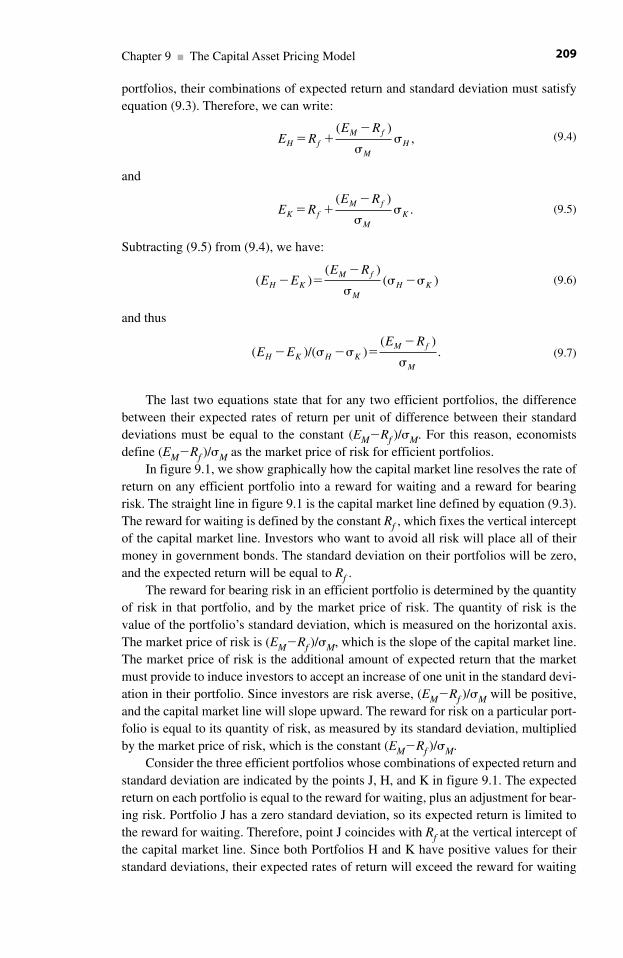
portfolios, their combinations of expected return and standard deviation must satisfyequation (9.3). Therefore, we can write:

(9.4)

and

(9.5)

Subtracting (9.5) from (9.4), we have:

(9.6)

and thus

(9.7)

The last two equations state that for any two efficient portfolios, the differencebetween their expected rates of return per unit of difference between their standarddeviations must be equal to the constant (EM�Rf )/ M. For this reason, economistsdefine (EM�Rf )/ M as the market price of risk for efficient portfolios.

In figure 9.1, we show graphically how the capital market line resolves the rate ofreturn on any efficient portfolio into a reward for waiting and a reward for bearingrisk. The straight line in figure 9.1 is the capital market line defined by equation (9.3).The reward for waiting is defined by the constant Rf , which fixes the vertical interceptof the capital market line. Investors who want to avoid all risk will place all of theirmoney in government bonds. The standard deviation on their portfolios will be zero,and the expected return will be equal to Rf .

The reward for bearing risk in an efficient portfolio is determined by the quantityof risk in that portfolio, and by the market price of risk. The quantity of risk is thevalue of the portfolio’s standard deviation, which is measured on the horizontal axis.The market price of risk is (EM�Rf )/ M, which is the slope of the capital market line.The market price of risk is the additional amount of expected return that the marketmust provide to induce investors to accept an increase of one unit in the standard devi-ation in their portfolio. Since investors are risk averse, (EM�Rf )/ M will be positive,and the capital market line will slope upward. The reward for risk on a particular port-folio is equal to its quantity of risk, as measured by its standard deviation, multipliedby the market price of risk, which is the constant (EM�Rf )/ M.

Consider the three efficient portfolios whose combinations of expected return andstandard deviation are indicated by the points J, H, and K in figure 9.1. The expectedreturn on each portfolio is equal to the reward for waiting, plus an adjustment for bear-ing risk. Portfolio J has a zero standard deviation, so its expected return is limited tothe reward for waiting. Therefore, point J coincides with Rf at the vertical intercept ofthe capital market line. Since both Portfolios H and K have positive values for theirstandard deviations, their expected rates of return will exceed the reward for waiting

( )/( )( )

.E EE R

H K H KM f

M

� � ��

( )( )

( )E EE R

H KM f

MH K� �

�

�

E RE R

K fM f

MK� �

�

( ).

E RE R

H fM f

H� ��

( ),

M


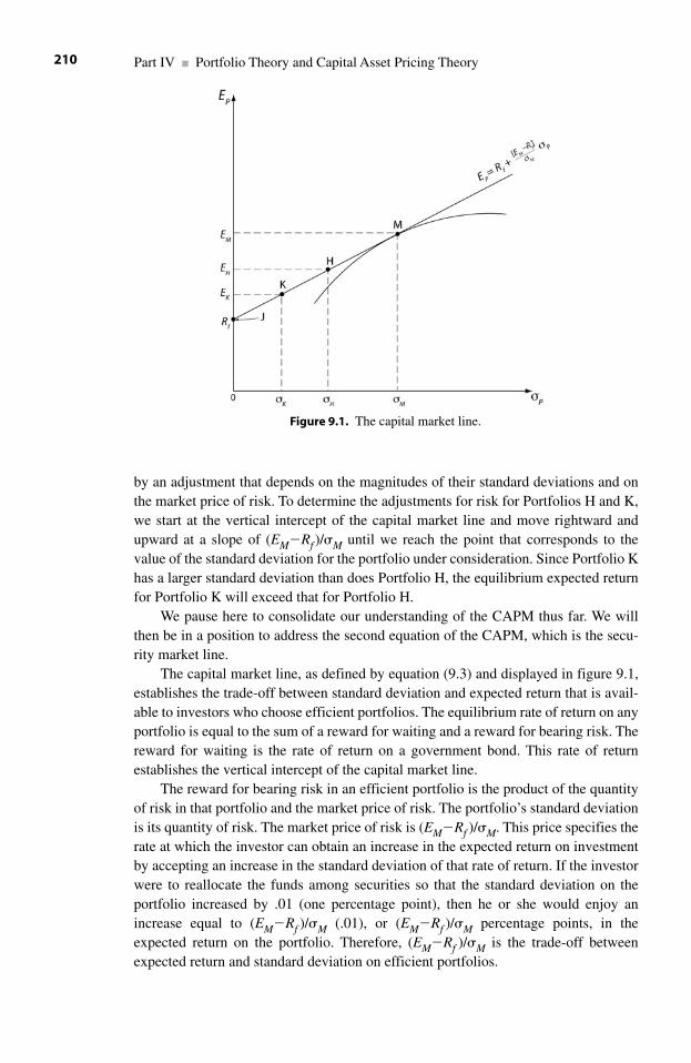
by an adjustment that depends on the magnitudes of their standard deviations and onthe market price of risk. To determine the adjustments for risk for Portfolios H and K,we start at the vertical intercept of the capital market line and move rightward andupward at a slope of (EM�Rf )/ M until we reach the point that corresponds to thevalue of the standard deviation for the portfolio under consideration. Since Portfolio Khas a larger standard deviation than does Portfolio H, the equilibrium expected returnfor Portfolio K will exceed that for Portfolio H.

We pause here to consolidate our understanding of the CAPM thus far. We willthen be in a position to address the second equation of the CAPM, which is the secu-rity market line.

The capital market line, as defined by equation (9.3) and displayed in figure 9.1,establishes the trade-off between standard deviation and expected return that is avail-able to investors who choose efficient portfolios. The equilibrium rate of return on anyportfolio is equal to the sum of a reward for waiting and a reward for bearing risk. Thereward for waiting is the rate of return on a government bond. This rate of returnestablishes the vertical intercept of the capital market line.

The reward for bearing risk in an efficient portfolio is the product of the quantityof risk in that portfolio and the market price of risk. The portfolio’s standard deviationis its quantity of risk. The market price of risk is (EM�Rf )/ M. This price specifies therate at which the investor can obtain an increase in the expected return on investmentby accepting an increase in the standard deviation of that rate of return. If the investorwere to reallocate the funds among securities so that the standard deviation on theportfolio increased by .01 (one percentage point), then he or she would enjoy anincrease equal to (EM�Rf )/ M (.01), or (EM�Rf )/ M percentage points, in theexpected return on the portfolio. Therefore, (EM�Rf )/ M is the trade-off betweenexpected return and standard deviation on efficient portfolios.


Figure 9.1. The capital market line.

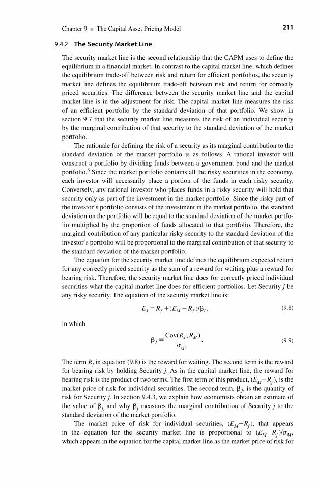
9.4.2 The Security Market Line

The security market line is the second relationship that the CAPM uses to define theequilibrium in a financial market. In contrast to the capital market line, which definesthe equilibrium trade-off between risk and return for efficient portfolios, the securitymarket line defines the equilibrium trade-off between risk and return for correctlypriced securities. The difference between the security market line and the capital market line is in the adjustment for risk. The capital market line measures the risk of an efficient portfolio by the standard deviation of that portfolio. We show in section 9.7 that the security market line measures the risk of an individual security by the marginal contribution of that security to the standard deviation of the marketportfolio.

The rationale for defining the risk of a security as its marginal contribution to thestandard deviation of the market portfolio is as follows. A rational investor willconstruct a portfolio by dividing funds between a government bond and the marketportfolio.5 Since the market portfolio contains all the risky securities in the economy,each investor will necessarily place a portion of the funds in each risky security.Conversely, any rational investor who places funds in a risky security will hold thatsecurity only as part of the investment in the market portfolio. Since the risky part ofthe investor’s portfolio consists of the investment in the market portfolio, the standarddeviation on the portfolio will be equal to the standard deviation of the market portfo-lio multiplied by the proportion of funds allocated to that portfolio. Therefore, themarginal contribution of any particular risky security to the standard deviation of theinvestor’s portfolio will be proportional to the marginal contribution of that security tothe standard deviation of the market portfolio.

The equation for the security market line defines the equilibrium expected returnfor any correctly priced security as the sum of a reward for waiting plus a reward forbearing risk. Therefore, the security market line does for correctly priced individualsecurities what the capital market line does for efficient portfolios. Let Security j beany risky security. The equation of the security market line is:

(9.8)

in which

(9.9)

The term Rf in equation (9.8) is the reward for waiting. The second term is the rewardfor bearing risk by holding Security j. As in the capital market line, the reward forbearing risk is the product of two terms. The first term of this product, (EM�Rf ), is themarket price of risk for individual securities. The second term, �J, is the quantity ofrisk for Security j. In section 9.4.3, we explain how economists obtain an estimate ofthe value of �j, and why �j measures the marginal contribution of Security j to thestandard deviation of the market portfolio.

The market price of risk for individual securities, (EM�Rf ), that appears in the equation for the security market line is proportional to (EM�Rf )/ M,which appears in the equation for the capital market line as the market price of risk for

�

JJ M

M

R R�

Cov( , ).

2

E R E RJ f M f J� � � �( )/ ,


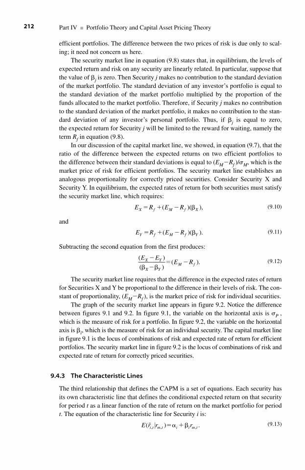
efficient portfolios. The difference between the two prices of risk is due only to scal-ing; it need not concern us here.

The security market line in equation (9.8) states that, in equilibrium, the levels ofexpected return and risk on any security are linearly related. In particular, suppose thatthe value of �j is zero. Then Security j makes no contribution to the standard deviationof the market portfolio. The standard deviation of any investor’s portfolio is equal tothe standard deviation of the market portfolio multiplied by the proportion of thefunds allocated to the market portfolio. Therefore, if Security j makes no contributionto the standard deviation of the market portfolio, it makes no contribution to the stan-dard deviation of any investor’s personal portfolio. Thus, if �j is equal to zero,the expected return for Security j will be limited to the reward for waiting, namely theterm Rf in equation (9.8).

In our discussion of the capital market line, we showed, in equation (9.7), that theratio of the difference between the expected returns on two efficient portfolios tothe difference between their standard deviations is equal to (EM�Rf )/ M, which is themarket price of risk for efficient portfolios. The security market line establishes ananalogous proportionality for correctly priced securities. Consider Security X andSecurity Y. In equilibrium, the expected rates of return for both securities must satisfythe security market line, which requires:

(9.10)

and

(9.11)

Subtracting the second equation from the first produces:

(9.12)

The security market line requires that the difference in the expected rates of returnfor Securities X and Y be proportional to the difference in their levels of risk. The con-stant of proportionality, (EM�Rf ), is the market price of risk for individual securities.

The graph of the security market line appears in figure 9.2. Notice the differencebetween figures 9.1 and 9.2. In figure 9.1, the variable on the horizontal axis is P ,which is the measure of risk for a portfolio. In figure 9.2, the variable on the horizontalaxis is �i, which is the measure of risk for an individual security. The capital market linein figure 9.1 is the locus of combinations of risk and expected rate of return for efficientportfolios. The security market line in figure 9.2 is the locus of combinations of risk andexpected rate of return for correctly priced securities.

9.4.3 The Characteristic Lines

The third relationship that defines the CAPM is a set of equations. Each security hasits own characteristic line that defines the conditional expected return on that securityfor period t as a linear function of the rate of return on the market portfolio for periodt. The equation of the characteristic line for Security i is:

(9.13)E r r ri t m t i i m t( ), , ,� ⏐ �� .

( )

( )( ).

E EE RX Y

X YM f

�

� ��

E R E RY f M f Y� � � �( )( ).

E R E RX f M f X� � � �( )( ),


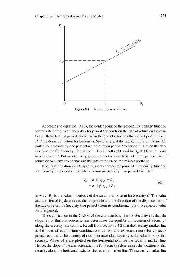
According to equation (9.13), the center point of the probability density functionfor the rate of return on Security i for period t depends on the rate of return on the mar-ket portfolio for that period. A change in the rate of return on the market portfolio willshift the density function for Security i. Specifically, if the rate of return on the marketportfolio increases by one percentage point from period t to period t�1, then the den-sity function for Security i for period t�1 will shift rightward by �i(.01) from its posi-tion in period t. Put another way, �i measures the sensitivity of the expected rate ofreturn on Security i to changes in the rate of return on the market portfolio.

Note that equation (9.13) specifies only the center point of the density functionfor Security i in period t. The rate of return on Security i for period t will be:

(9.14)

in which ei,t is the value in period t of the random error term for Security i.6 The valueand the sign of ei,t determines the magnitude and the direction of the displacement ofthe rate of return on Security i for period t from its conditional (on rm,t) expected valuefor that period.

The significance in the CAPM of the characteristic line for Security i is that theslope, �i, of that characteristic line determines the equilibrium location of Security ialong the security market line. Recall from section 9.4.2 that the security market lineis the locus of equilibrium combinations of risk and expected return for correctlypriced securities. The quantity of risk in an individual security is the value of � for thatsecurity. Values of � are plotted on the horizontal axis for the security market line.Hence, the slope of the characteristic line for Security i determines the location of thatsecurity along the horizontal axis for the security market line. The security market line

� � �

�

r E r r e

r ei t i t m t i t

i i m t i t

, , , ,

, ,

[ ]

,

� �

� � ��

⏐


0 β i

E i

E M

R f

1

E i= R f

+ (E M−R f

) β i

Figure 9.2. The security market line.

then determines the equilibrium expected return for Security i that is compatible withthe quantity of risk contained in Security i. The values of αi and �i in the characteris-tic line for Security i are estimated by using historical data to regress ri on rm.

9.5 A Summary of the Intuitive Introduction to the CAPM

The CAPM defines equilibrium for both efficient portfolios and for correctly pricedindividual securities. In each case, the equilibrium expected rate of return is equal to areward for waiting plus a reward for bearing risk. The reward for waiting is the inter-est that an investor foregoes by not having money in a government bond. This oppor-tunity cost is the same for efficient portfolios and for correctly priced securities. It is the constant that appears as the first term in both the capital market line and thesecurity market line.

With regard to risk, each investor is ultimately interested in the unpredictablevariability of the rate of return on his or her personal portfolio. Therefore theinvestor’s reward for bearing risk, whether at the level of the portfolio or at the levelof an individual security held in that portfolio, depends on the standard deviation ofthe portfolio. In either case, the reward for bearing risk is equal to a market price ofrisk multiplied by a quantity of risk. These market prices of risk establish the trade-offs that the investor can make between an increase in the level of risk and theincrease in the level of expected return that the market will provide as compensationfor that increase in risk.

For the investor’s personal portfolio, the quantity of risk is equal to the proportionof funds in the market portfolio multiplied by the standard deviation on the marketportfolio. For an individual security, the quantity of risk is equal to that security’s mar-ginal contribution to the standard deviation of the market portfolio, because everyinvestor places some funds in the market portfolio, and the market portfolio containsevery risky security.

The fact that both the capital market line and the security market line are linearmakes it easy to obtain clear economic interpretations of the equilibrium that thecapital asset pricing model predicts for a financial market. We shall examine theseinterpretations in detail later in this chapter. These economic interpretations are usefulfor understanding how financial markets allocate resources between production forthe present and production for the future. We can then use this understanding to ana-lyze questions of public policy regarding financial markets.

The usefulness of theoretical models, particularly as a guide to policy, depends onempirical verification of those models. The empirical implications of the capital assetpricing model are relatively easy to test empirically because the equations for the cap-ital market line and the security market line are linear. Economists have conducted alarge number of empirical studies of the CAPM. We shall see that the results of thesetests have contributed much to our understanding of how financial markets set theprices of securities. We shall also see how the failures of the CAPM to explain certainphenomena (such as the relationship between risk and expected return for small firms)have led to more sophisticated models of asset pricing.


9.6 The Derivation of the Capital Market Line

9.6.1 The Assumptions

The derivation of the capital market line is based on several assumptions. As with anyeconomic model, we should judge the CAPM not by the realism of its assumptions,but by its ability to organize thinking, to produce insights, and to generate empiricallytestable hypotheses. The assumptions are as follows:

1. There is a risk-free asset that provides a guaranteed rate of return.2. There are no restrictions against selling short.3. There are no transaction costs or taxes.4. Every investor evaluates a portfolio solely on the basis of its combination of

expected return and standard deviation. 5. Investors are risk averse in the following sense. If two portfolios have the

same value for their expected returns, investors will prefer the portfolio thathas the lower value for its standard deviation. Similarly, if two portfolios havethe same value for their standard deviations, investors will prefer the portfoliothat has the higher value for its expected return.

6. All investors have the same beliefs about the values of the expected returnsand the standard deviations for all individual securities, and the correlationcoefficients between all pairs of securities. Therefore the locus of combina-tions of expected return and standard deviation for efficient portfolios is thesame for all investors.

9.6.2 A Digression on the Use of Assumptions in Economics

There is frequently a misunderstanding about why economists make assumptions.Since the derivation of capital market theory is also based on assumptions, we digressfor a moment to discuss the use of assumptions in economics.7

The ultimate objective in microeconomic theory is to establish knowledge abouthow markets set prices. This means that we must be able to identify the fundamentalvariables that determine prices. We must also be able to predict how the market willchange those prices if the values of those fundamental variables change. There is animportant distinction here that is frequently ignored, or at least misunderstood, bypersons who have not studied economics formally. The object of economics is not topredict the values of the fundamental variables and thus the values of the prices.Rather, the object is to explain the relationship between the fundamental variables andthe prices.

For example, suppose that the market for apples is perfectly competitive. Supposealso that the demand curve for apples slopes downward, and the supply curve forapples slopes upward (their usual shapes). Economic theory should be able to answerthe question: “What would be the effect on the price of apples of a tax on suppliersequal to $2 per bushel of apples sold?” Economic theory is not responsible for predict-ing the price of apples. The theory is responsible for only predicting the change in theprice of apples if the tax is imposed.


The operation of a market economy in setting prices and allocating resources ishighly complex. The number of individuals involved is large, and these individualsdiffer in the quality of their information, their objectives, and their personal resources.The complexity of the markets makes it difficult for economists to generate hypothe-ses that are both highly detailed and empirically testable. A highly detailed descriptionof an individual investor, for example, might be very interesting, but the very com-plexity of the detail that makes the description interesting also inhibits analysis. Amodel that is realistic is usually too complex to allow the economist to answer ques-tions that take the form, “What would happen to X if Y were to change?”

To analyze a market system (or any system) is to answer questions that take theform: “What would happen if . . .” In analyzing a market system, economists managethe problem of complexity by basing their initial analysis on assumptions on howindividuals make choices. In making these assumptions, we are not attempting todescribe the conscious thought processes of every individual, although it would cer-tainly be useful (and fascinating) if we could do so. Rather, the purpose of the assump-tions is to enable economists to use the powerful methods of mathematics to deriveempirically testable hypotheses about how markets set prices. The validity of theseassumptions is determined not by how accurately they describe how an individualwould explain how he or she makes choices. Rather, the validity of a set of assump-tions depends on the success with which economists, using these assumptions, canderive hypotheses that are eventually verified by empirical testing.

Starting with their tentative assumptions about how individuals make choicesgenerally, economists use logic, usually by analyzing formal mathematical models, toderive theoretical propositions to describe how an individual’s specific choices wouldbe related to specific factors beyond his or her control. The next step is to determinewhat would happen if all individuals in a given market made their choices in this way.The final step is to derive empirically testable hypotheses based on the behavior pre-dicted by the theory. If the hypotheses are supported by the empirical tests, then econ-omists can place some confidence in the initial assumptions from which the theory,and then the empirical hypotheses, were derived.

9.6.3 Constructing the Capital Market Line

We can now construct the capital market line, which will define the equilibrium trade-off between expected return and standard deviation for efficient portfolios. The firststep is to represent a portfolio as a point in a two-dimensional space.

Associated with any portfolio is the probability density function that generatesvalues for the rate of return on that portfolio. That probability density function is com-pletely defined by the values of its expected return and standard deviation. Therefore,we can represent a particular portfolio by a single point in a graph in which the stan-dard deviation is measured along the horizontal axis, and the expected return is meas-ured along the vertical axis.

Let there be a total of N risky securities in the economy. In figure 9.3, the curvedlocus is the boundary of the combinations of expected return and standard deviationthat an investor can obtain by constructing portfolios that contain only risky securities.We explained in chapter 8 why this locus is concave. Portfolios such as D, which lie


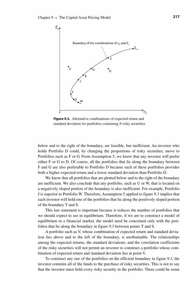
below and to the right of the boundary, are feasible, but inefficient. An investor whoholds Portfolio D could, by changing the proportions of risky securities, move toPortfolios such as F or G. From Assumption 5, we know that any investor will prefereither F or G to D. Of course, all the portfolios that lie along the boundary betweenF and G are also preferable to Portfolio D because each of these portfolios providesboth a higher expected return and a lower standard deviation than Portfolio D.

We know that all portfolios that are plotted below and to the right of the boundaryare inefficient. We also conclude that any portfolio, such as U or W, that is located ona negatively sloped portion of the boundary is also inefficient. For example, PortfolioJ is superior to Portfolio W. Therefore, Assumption 5 applied to figure 9.3 implies thateach investor will hold one of the portfolios that lie along the positively sloped portionof the boundary T and S.

This last statement is important because it reduces the number of portfolios thatwe should expect to see in equilibrium. Therefore, if we are to construct a model ofequilibrium in a financial market, the model need be concerned only with the port-folios that lie along the boundary in figure 9.3 between points T and S.

A portfolio such as V, whose combination of expected return and standard devia-tion lies above and to the left of the boundary, is unobtainable. The relationshipsamong the expected returns, the standard deviations, and the correlation coefficientsof the risky securities will not permit an investor to construct a portfolio whose com-bination of expected return and standard deviation lies at point V.

To construct any one of the portfolios on the efficient boundary in figure 9.3, theinvestor commits all of the funds to the purchase of risky securities. This is not to saythat the investor must hold every risky security in the portfolio. There could be some


Figure 9.3. Alternative combinations of expected return andstandard deviation for portfolios containing N risky securities.

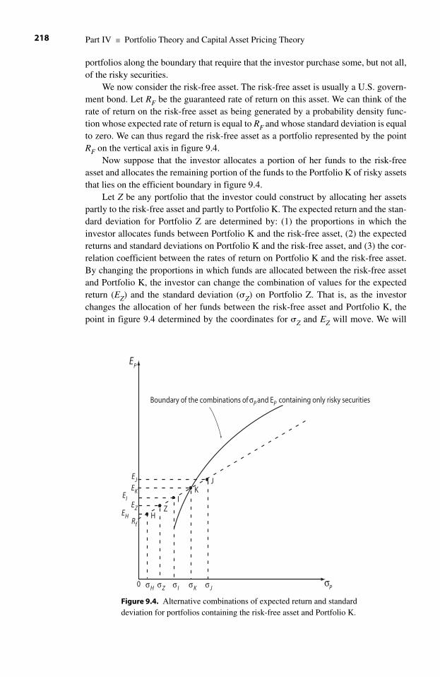
portfolios along the boundary that require that the investor purchase some, but not all,of the risky securities.

We now consider the risk-free asset. The risk-free asset is usually a U.S. govern-ment bond. Let RF be the guaranteed rate of return on this asset. We can think of therate of return on the risk-free asset as being generated by a probability density func-tion whose expected rate of return is equal to RF and whose standard deviation is equalto zero. We can thus regard the risk-free asset as a portfolio represented by the pointRF on the vertical axis in figure 9.4.

Now suppose that the investor allocates a portion of her funds to the risk-freeasset and allocates the remaining portion of the funds to the Portfolio K of risky assetsthat lies on the efficient boundary in figure 9.4.

Let Z be any portfolio that the investor could construct by allocating her assetspartly to the risk-free asset and partly to Portfolio K. The expected return and the stan-dard deviation for Portfolio Z are determined by: (1) the proportions in which theinvestor allocates funds between Portfolio K and the risk-free asset, (2) the expectedreturns and standard deviations on Portfolio K and the risk-free asset, and (3) the cor-relation coefficient between the rates of return on Portfolio K and the risk-free asset.By changing the proportions in which funds are allocated between the risk-free assetand Portfolio K, the investor can change the combination of values for the expectedreturn (EZ) and the standard deviation ( Z) on Portfolio Z. That is, as the investorchanges the allocation of her funds between the risk-free asset and Portfolio K, thepoint in figure 9.4 determined by the coordinates for Z and EZ will move. We will


0 σP

EP

Boundary of the combinations of σP and EP

KJ

H

IZ

EK

EZEH

σH σZ σ I σK σJ

EI

EJ

Rf

containing only risky securities

Figure 9.4. Alternative combinations of expected return and standarddeviation for portfolios containing the risk-free asset and Portfolio K.

now derive the equation that specifies the trade-off between values for the expectedreturn and values for the standard deviation on Portfolio Z.

Let Xrf and Xk be the proportions in which the investor allocates funds betweenthe risk-free asset and Portfolio K in order to form Portfolio Z. We have Xrf�Xk�1because Portfolio Z contains only the risk-free asset and Portfolio K.

In chapter 8, we used equations (8.5) and (8.6) to obtain the expected return andthe standard deviation for a portfolio that contains two securities. Repeating those twoequations here, and applying them to Portfolio Z, we have:

Ez�Xrf E(rf )�XkEk, (9.15)

and

( Z)2�(Xrf rf )2�2Xrf Xk �rf ,k rf k� (Xk k)

2. (9.16)

The middle term in equation (9.16) contains the expression �rf rf k. By defini-tion of a correlation coefficient, we have ρrf,k�Cov(rf ,rk)/ rf k, in which Cov(rf ,rk)is the covariance between the rates of return on the risk-free asset and the market port-folio. Since the standard deviation on the risk-free asset, rf , is equal to zero, the cor-relation coefficient between the risk-free asset and Portfolio K is undefined. For thisreason, we rewrite equation (9.16) as

( Z)2�(Xrf rf)2�2Xrf XkCov(rf ,rk)�(Xk k)

2. (9.17)

By definition, the standard deviation of the risk-free asset is equal to zero. Thecovariance between the rate of return on the risk-free asset and the rate of return onPortfolio K is also equal to zero. A covariance is a measure of the relationship betweenchanges in one variable and changes in a second variable. Specifically, the covariancebetween the rates of return on the risk-free asset and Portfolio K is a probability-weighted sum of products. Each product is a deviation of the rate of return on the risk-free asset from the expected rate of return on that asset, multiplied by a deviation ofthe rate of return on Portfolio K from the expected rate of return on Portfolio K. Butby definition, the rate of return on the risk-free asset never deviates from its expectedvalue. Therefore, every product in the sum that defines the covariance between therisk-free asset and Portfolio K contains a zero. Hence the entire sum, and thus thecovariance between the risk-free asset and Portfolio K, is equal to zero.

Since both the standard deviation of the risk-free asset and the covariancebetween the risk-free asset and Portfolio K are equal to zero, the first two terms on theright-hand side of equation (9.17) are equal to zero. Taking the positive square rootson both sides of (9.17) produces:

z�Xk k. (9.18)

Solving (9.18) for Xk, we obtain:

(9.19)

Since Xrf � Xk�1, we can write Xrf�1�Xk. Using Xk� z/ k, we can write:

(9.20)

X Xrf k

z k

k z k

� �

� �

� �

1

1 /

( )/ .

/ .k z kX ��


Finally, using (9.15) and (9.20), we can rewrite (9.15) as:

(9.21)

(9.22)

Equation (9.22) is the equation of a straight line. The variables are the expectedreturn and the standard deviation of a portfolio constructed by allocating fundsbetween the risk-free asset and Portfolio K. Three of these portfolios are designatedby the points H, I, and J in figure 9.4. The relative locations of these points indicatehow the three portfolios differ in their dependence on the risk-free asset and PortfolioK. Specifically, let Xh, Xi, and Xj be the proportions of the investor’s initial funds allo-cated to the risk-free asset to form Portfolios H, I, and J. Using equations (9.22) and(9.19), we can show that 1�Xh�Xi � Xj.

Consider Portfolio H, and let EH and H be the expected rate of return and thestandard deviation on that portfolio. Since Portfolio H lies strictly between point Rfand point K in figure 9.4, we have Rf EH EK. Since the expected return and thestandard deviation for Portfolio H must satisfy (9.22), we have:

(9.23)

In figure 9.4, EK�Rf . Then the inequality on the left in equation (9.23) requires that H/ K � 0, and the inequality on the right requires that H/ K 1. Thenequation (9.19) requires that 1�Xh�0. Similar arguments will establish that1�Xh�Xi�0�Xj.

Since Portfolios H, I, and J contain only the risk-free asset and Portfolio K, theproportions of the investor’s initial funds allocated to Portfolio K in each case areequal to 1 minus the proportions allocated to the risk-free asset. Then the relative posi-tions of Portfolios H, I, and J in figure 9.4 imply that 1�Xj�1�1�Xi�1�Xh�0.

To form either Portfolio H or Portfolio I, the investor holds long positions in boththe risk-free asset and in Portfolio K. Portfolio J lies beyond point K in figure 9.4.To form Portfolio J, the investor must sell the risk-free asset short and allocate toPortfolio K 100% of the initial funds plus the funds raised from the short sale of therisk-free asset.

The next step in constructing the capital market line is to recognize that the con-cavity of the efficient frontier of portfolios that contain only risky securities meansthat there is a unique optimal portfolio of risky securities that an investor should com-bine with the risk-free asset. This portfolio is located at the point of tangency betweenthe straight line that emanates from Rf on the vertical axis and that is tangential to theefficient boundary for portfolios that contain only risky securities. This tangential lineis the capital market line, which we have drawn and so labeled in figure 9.5. Designatethe point of tangency as point M, which corresponds to a specific portfolio of riskysecurities known as the market portfolio.

R RE R

Ef fK f

KH K �

�

⎡

⎣⎢

⎤

⎦⎥ .

E RE R

z fk f

kz� �

�

( ).

E R EzK Z

Kf

K Z

KK�

�

� �

�

⎡

⎣⎢

⎤

⎦⎥

⎡

⎣⎢

⎤

⎦⎥

⎡

⎣⎢

⎤

⎦⎥


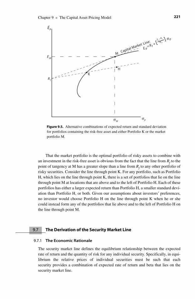
That the market portfolio is the optimal portfolio of risky assets to combine withan investment in the risk-free asset is obvious from the fact that the line from Rf to thepoint of tangency at M has a greater slope than a line from Rf to any other portfolio ofrisky securities. Consider the line through point K. For any portfolio, such as PortfolioH, which lies on the line through point K, there is a set of portfolios that lie on the linethrough point M at locations that are above and to the left of Portfolio H. Each of theseportfolios has either a larger expected return than Portfolio H, a smaller standard devi-ation than Portfolio H, or both. Given our assumptions about investors’ preferences,no investor would choose Portfolio H on the line through point K when he or shecould instead form any of the portfolios that lie above and to the left of Portfolio H onthe line through point M.

9.7 The Derivation of the Security Market Line

9.7.1 The Economic Rationale

The security market line defines the equilibrium relationship between the expectedrate of return and the quantity of risk for any individual security. Specifically, in equi-librium the relative prices of individual securities must be such that each security provides a combination of expected rate of return and beta that lies on thesecurity market line.


σP

EP

K

M Capital Market Line:

H

E M

σM

R f

E p = R f

+ [] σ pE m

−R f

σ m

Figure 9.5. Alternative combinations of expected return and standard deviationfor portfolios containing the risk-free asset and either Portfolio K or the marketportfolio M.

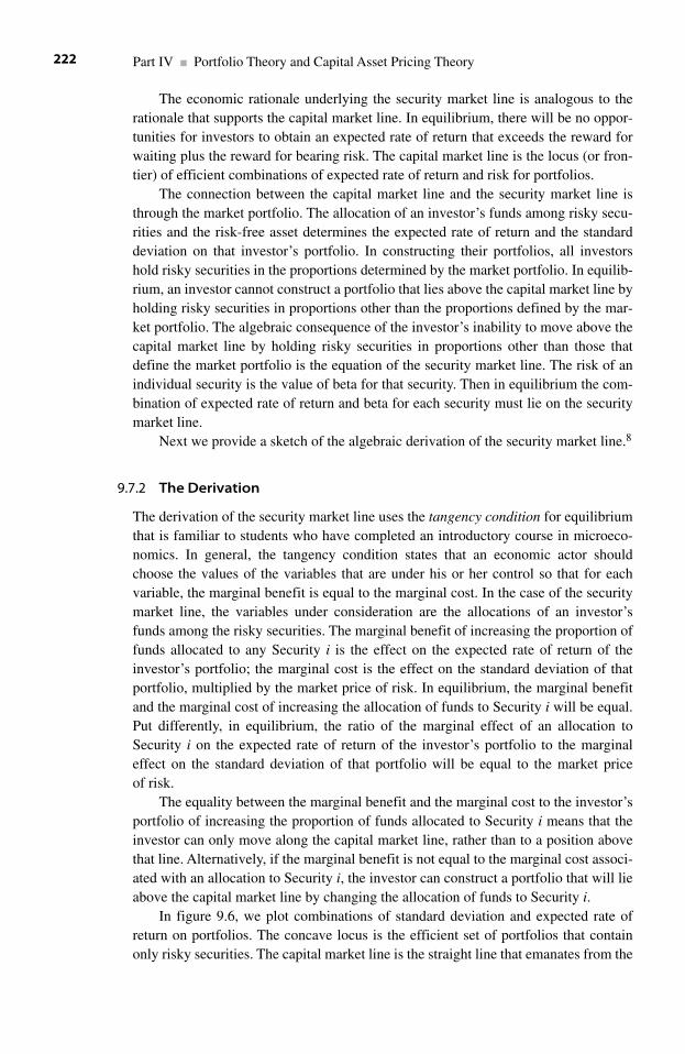
The economic rationale underlying the security market line is analogous to therationale that supports the capital market line. In equilibrium, there will be no oppor-tunities for investors to obtain an expected rate of return that exceeds the reward forwaiting plus the reward for bearing risk. The capital market line is the locus (or fron-tier) of efficient combinations of expected rate of return and risk for portfolios.

The connection between the capital market line and the security market line isthrough the market portfolio. The allocation of an investor’s funds among risky secu-rities and the risk-free asset determines the expected rate of return and the standarddeviation on that investor’s portfolio. In constructing their portfolios, all investorshold risky securities in the proportions determined by the market portfolio. In equilib-rium, an investor cannot construct a portfolio that lies above the capital market line byholding risky securities in proportions other than the proportions defined by the mar-ket portfolio. The algebraic consequence of the investor’s inability to move above thecapital market line by holding risky securities in proportions other than those thatdefine the market portfolio is the equation of the security market line. The risk of anindividual security is the value of beta for that security. Then in equilibrium the com-bination of expected rate of return and beta for each security must lie on the securitymarket line.

Next we provide a sketch of the algebraic derivation of the security market line.8

9.7.2 The Derivation

The derivation of the security market line uses the tangency condition for equilibriumthat is familiar to students who have completed an introductory course in microeco-nomics. In general, the tangency condition states that an economic actor shouldchoose the values of the variables that are under his or her control so that for eachvariable, the marginal benefit is equal to the marginal cost. In the case of the securitymarket line, the variables under consideration are the allocations of an investor’sfunds among the risky securities. The marginal benefit of increasing the proportion offunds allocated to any Security i is the effect on the expected rate of return of theinvestor’s portfolio; the marginal cost is the effect on the standard deviation of thatportfolio, multiplied by the market price of risk. In equilibrium, the marginal benefitand the marginal cost of increasing the allocation of funds to Security i will be equal.Put differently, in equilibrium, the ratio of the marginal effect of an allocation toSecurity i on the expected rate of return of the investor’s portfolio to the marginaleffect on the standard deviation of that portfolio will be equal to the market price of risk.

The equality between the marginal benefit and the marginal cost to the investor’sportfolio of increasing the proportion of funds allocated to Security i means that theinvestor can only move along the capital market line, rather than to a position abovethat line. Alternatively, if the marginal benefit is not equal to the marginal cost associ-ated with an allocation to Security i, the investor can construct a portfolio that will lieabove the capital market line by changing the allocation of funds to Security i.

In figure 9.6, we plot combinations of standard deviation and expected rate ofreturn on portfolios. The concave locus is the efficient set of portfolios that containonly risky securities. The capital market line is the straight line that emanates from the


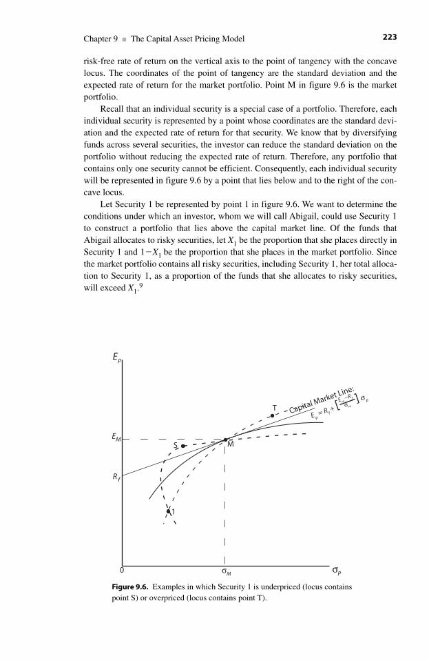
risk-free rate of return on the vertical axis to the point of tangency with the concavelocus. The coordinates of the point of tangency are the standard deviation and theexpected rate of return for the market portfolio. Point M in figure 9.6 is the marketportfolio.

Recall that an individual security is a special case of a portfolio. Therefore, eachindividual security is represented by a point whose coordinates are the standard devi-ation and the expected rate of return for that security. We know that by diversifyingfunds across several securities, the investor can reduce the standard deviation on theportfolio without reducing the expected rate of return. Therefore, any portfolio thatcontains only one security cannot be efficient. Consequently, each individual securitywill be represented in figure 9.6 by a point that lies below and to the right of the con-cave locus.

Let Security 1 be represented by point 1 in figure 9.6. We want to determine theconditions under which an investor, whom we will call Abigail, could use Security 1to construct a portfolio that lies above the capital market line. Of the funds thatAbigail allocates to risky securities, let X1 be the proportion that she places directly inSecurity 1 and 1�X1 be the proportion that she places in the market portfolio. Sincethe market portfolio contains all risky securities, including Security 1, her total alloca-tion to Security 1, as a proportion of the funds that she allocates to risky securities,will exceed X1.9


σP

EP

T

MS

1

EM

σM

R f

0

Capital Market Line:

E p = R f

+ [] σ pE m

−R f

σ m

Figure 9.6. Examples in which Security 1 is underpriced (locus containspoint S) or overpriced (locus contains point T).

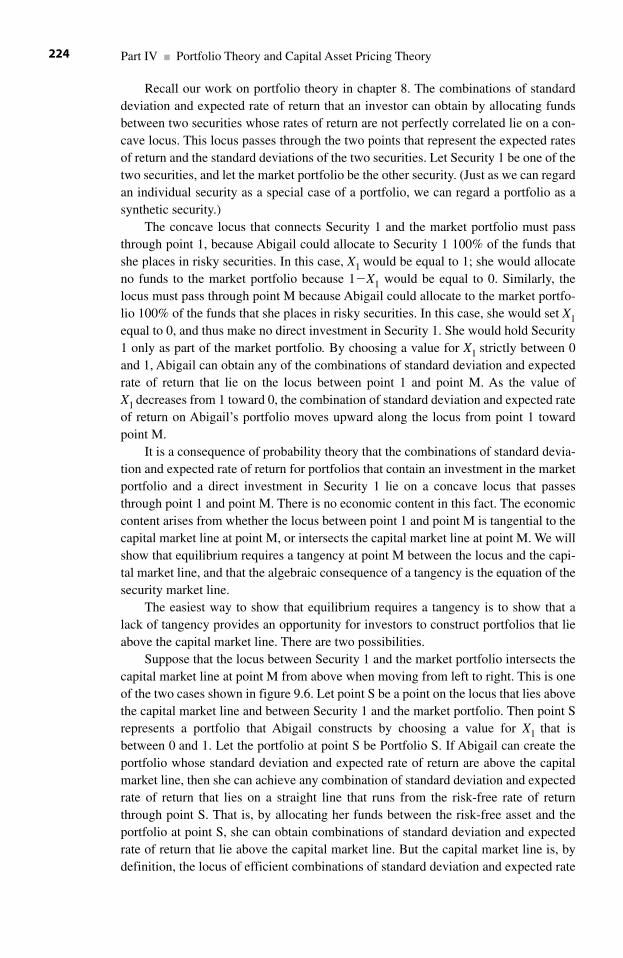
Recall our work on portfolio theory in chapter 8. The combinations of standarddeviation and expected rate of return that an investor can obtain by allocating fundsbetween two securities whose rates of return are not perfectly correlated lie on a con-cave locus. This locus passes through the two points that represent the expected ratesof return and the standard deviations of the two securities. Let Security 1 be one of thetwo securities, and let the market portfolio be the other security. (Just as we can regardan individual security as a special case of a portfolio, we can regard a portfolio as asynthetic security.)

The concave locus that connects Security 1 and the market portfolio must passthrough point 1, because Abigail could allocate to Security 1 100% of the funds thatshe places in risky securities. In this case, X1 would be equal to 1; she would allocateno funds to the market portfolio because 1�X1 would be equal to 0. Similarly, thelocus must pass through point M because Abigail could allocate to the market portfo-lio 100% of the funds that she places in risky securities. In this case, she would set X1equal to 0, and thus make no direct investment in Security 1. She would hold Security1 only as part of the market portfolio. By choosing a value for X1 strictly between 0and 1, Abigail can obtain any of the combinations of standard deviation and expectedrate of return that lie on the locus between point 1 and point M. As the value of X1 decreases from 1 toward 0, the combination of standard deviation and expected rateof return on Abigail’s portfolio moves upward along the locus from point 1 towardpoint M.

It is a consequence of probability theory that the combinations of standard devia-tion and expected rate of return for portfolios that contain an investment in the marketportfolio and a direct investment in Security 1 lie on a concave locus that passesthrough point 1 and point M. There is no economic content in this fact. The economiccontent arises from whether the locus between point 1 and point M is tangential to thecapital market line at point M, or intersects the capital market line at point M. We willshow that equilibrium requires a tangency at point M between the locus and the capi-tal market line, and that the algebraic consequence of a tangency is the equation of thesecurity market line.

The easiest way to show that equilibrium requires a tangency is to show that alack of tangency provides an opportunity for investors to construct portfolios that lieabove the capital market line. There are two possibilities.

Suppose that the locus between Security 1 and the market portfolio intersects thecapital market line at point M from above when moving from left to right. This is oneof the two cases shown in figure 9.6. Let point S be a point on the locus that lies abovethe capital market line and between Security 1 and the market portfolio. Then point Srepresents a portfolio that Abigail constructs by choosing a value for X1 that isbetween 0 and 1. Let the portfolio at point S be Portfolio S. If Abigail can create theportfolio whose standard deviation and expected rate of return are above the capitalmarket line, then she can achieve any combination of standard deviation and expectedrate of return that lies on a straight line that runs from the risk-free rate of returnthrough point S. That is, by allocating her funds between the risk-free asset and theportfolio at point S, she can obtain combinations of standard deviation and expectedrate of return that lie above the capital market line. But the capital market line is, bydefinition, the locus of efficient combinations of standard deviation and expected rate


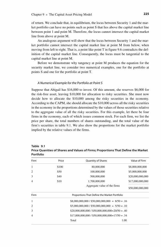
of return. We conclude that, in equilibrium, the locus between Security 1 and the mar-ket portfolio can have no points such as point S that lies above the capital market linebetween point 1 and point M. Therefore, the locus cannot intersect the capital marketline from above at point M.

An analogous argument will show that the locus between Security 1 and the mar-ket portfolio cannot intersect the capital market line at point M from below, whenmoving from left to right. That is, a point like point T in figure 9.6 contradicts the def-inition of the capital market line. Consequently, the locus must be tangential to thecapital market line at point M.

Before we demonstrate why tangency at point M produces the equation for thesecurity market line, we consider two numerical examples, one for the portfolio atpoints S and one for the portfolio at point T.

A Numerical Example for the Portfolio at Point S

Suppose that Abigail has $16,000 to invest. Of this amount, she reserves $6,000 forthe risk-free asset, leaving $10,000 for allocation to risky securities. She must nowdecide how to allocate the $10,000 among the risky securities in the economy.According to the CAPM, she should allocate the $10,000 across all the risky securitiesin the economy in the proportions determined by the values of those securities relativeto the aggregate value of all the risky securities. For this example, let there be fourfirms in the economy, each of which issues common stock. For each firm, we list theprice per share, the total numbers of shares outstanding, and the total value of thefirm’s securities in table 9.1. We also show the proportions for the market portfolioimplied by the relative values of the firms.


Table 9.1Price Quanities of Shares and Values of Firms; Proportions That Define the MarketPortfolio

Firm Price Quantity of Shares Value of Firm

1 $100 80,000,000 $8,000,000,000

2 $50 100,000,000 $5,000,000,000

3 $40 500,000,000 $20,000,000,000

4 $10 1,700,000,000 $17,000,000,000

Aggregate value of the firms$50,000,000,000

Firm Proportions That Define the Market Portfolio

1 $8,000,000,000 / $50,000,000,000 = 8/50 = .16

2 $5,000,000,000 / $50,000,000,000 = 5/50 = .10

3 $20,000,000,000 / $50,000,000,000=20/50 = .40

4 $17,000,000,000 / $50,000,000,000=17/50 = .34

Total 1.00

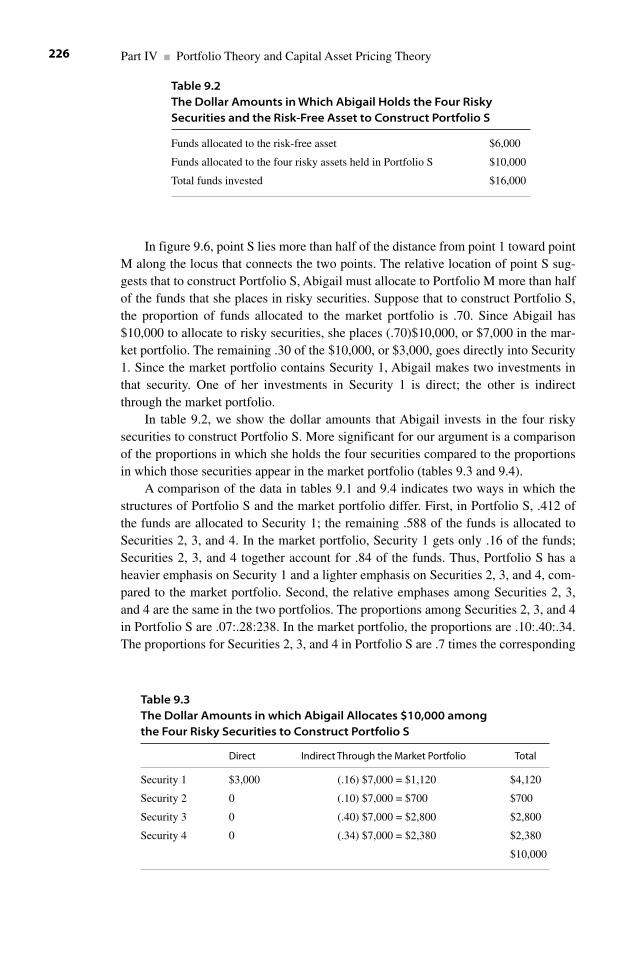
In figure 9.6, point S lies more than half of the distance from point 1 toward pointM along the locus that connects the two points. The relative location of point S sug-gests that to construct Portfolio S, Abigail must allocate to Portfolio M more than halfof the funds that she places in risky securities. Suppose that to construct Portfolio S,the proportion of funds allocated to the market portfolio is .70. Since Abigail has$10,000 to allocate to risky securities, she places (.70)$10,000, or $7,000 in the mar-ket portfolio. The remaining .30 of the $10,000, or $3,000, goes directly into Security1. Since the market portfolio contains Security 1, Abigail makes two investments inthat security. One of her investments in Security 1 is direct; the other is indirectthrough the market portfolio.

In table 9.2, we show the dollar amounts that Abigail invests in the four riskysecurities to construct Portfolio S. More significant for our argument is a comparisonof the proportions in which she holds the four securities compared to the proportionsin which those securities appear in the market portfolio (tables 9.3 and 9.4).

A comparison of the data in tables 9.1 and 9.4 indicates two ways in which thestructures of Portfolio S and the market portfolio differ. First, in Portfolio S, .412 ofthe funds are allocated to Security 1; the remaining .588 of the funds is allocated toSecurities 2, 3, and 4. In the market portfolio, Security 1 gets only .16 of the funds;Securities 2, 3, and 4 together account for .84 of the funds. Thus, Portfolio S has aheavier emphasis on Security 1 and a lighter emphasis on Securities 2, 3, and 4, com-pared to the market portfolio. Second, the relative emphases among Securities 2, 3,and 4 are the same in the two portfolios. The proportions among Securities 2, 3, and 4in Portfolio S are .07:.28:238. In the market portfolio, the proportions are .10:.40:.34.The proportions for Securities 2, 3, and 4 in Portfolio S are .7 times the corresponding


Table 9.2The Dollar Amounts in Which Abigail Holds the Four Risky Securities and the Risk-Free Asset to Construct Portfolio S

Funds allocated to the risk-free asset $6,000

Funds allocated to the four risky assets held in Portfolio S $10,000

Total funds invested $16,000

Table 9.3The Dollar Amounts in which Abigail Allocates $10,000 among the Four Risky Securities to Construct Portfolio S

Direct Indirect Through the Market Portfolio Total

Security 1 $3,000 (.16) $7,000 = $1,120 $4,120

Security 2 0 (.10) $7,000 = $700 $700

Security 3 0 (.40) $7,000 = $2,800 $2,800

Security 4 0 (.34) $7,000 = $2,380 $2,380

$10,000

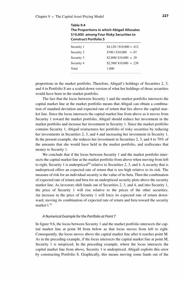
proportions in the market portfolio. Therefore, Abigail’s holdings of Securities 2, 3,and 4 in Portfolio S are a scaled-down version of what her holdings of those securitieswould have been in the market portfolio.

The fact that the locus between Security 1 and the market portfolio intersects thecapital market line at the market portfolio means that Abigail can obtain a combina-tion of standard deviation and expected rate of return that lies above the capital mar-ket line. Since the locus intersects the capital market line from above as it moves fromSecurity 1 toward the market portfolio, Abigail should reduce her investment in themarket portfolio and increase her investment in Security 1. Since the market portfoliocontains Security 1, Abigail restructures her portfolio of risky securities by reducingher investments in Securities 2, 3, and 4 and increasing her investment in Security 1.In the present example, she reduces her investment in Securities 2, 3, and 4 to 70% ofthe amounts that she would have held in the market portfolio, and reallocates thatmoney to Security 1.

We conclude that if the locus between Security 1 and the market portfolio inter-sects the capital market line at the market portfolio from above when moving from leftto right, Security 1 is underpriced10 relative to Securities 2, 3, and 4. A security that isunderpriced offers an expected rate of return that is too high relative to its risk. Themeasure of risk for an individual security is the value of its beta. Then the combinationof expected rate of return and beta for an underpriced security plots above the securitymarket line. As investors shift funds out of Securities 2, 3, and 4, and into Security 1,the price of Security 1 will rise relative to the prices of the other securities. An increase in the price of Security 1 will force its expected rate of return down-ward, moving its combination of expected rate of return and beta toward the securitymarket l.11

A Numerical Example for the Portfolio at Point T

In figure 9.6, the locus between Security 1 and the market portfolio intersects the cap-ital market line at point M from below as that locus moves from left to right.Consequently, the locus moves above the capital market line after it reaches point M.As in the preceding example, if the locus intersects the capital market line at point M,Security 1 is mispriced. In the preceding example, where the locus intersects the capital market line from above, Security 1 is underpriced. Abigail exploits this errorby constructing Portfolio S. Graphically, this means moving some funds out of the


Table 9.4The Proportions in which Abigail Allocates $10,000 among Four Risky Securities to Construct Portfolio S

Security 1 $4,120 / $10,000 = .412

Security 2 $700 / $10,000 = .07

Security 3 $2,800/ $10,000 = .28

Security 4 $2,380/ $10,000 = .238

Total 1.000

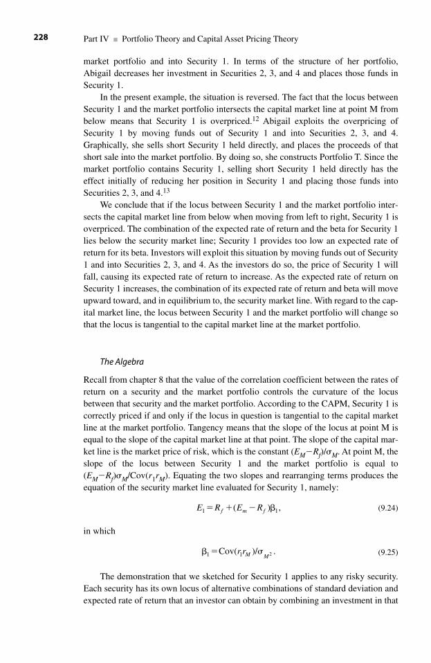
market portfolio and into Security 1. In terms of the structure of her portfolio, Abigail decreases her investment in Securities 2, 3, and 4 and places those funds inSecurity 1.

In the present example, the situation is reversed. The fact that the locus betweenSecurity 1 and the market portfolio intersects the capital market line at point M frombelow means that Security 1 is overpriced.12 Abigail exploits the overpricing ofSecurity 1 by moving funds out of Security 1 and into Securities 2, 3, and 4.Graphically, she sells short Security 1 held directly, and places the proceeds of thatshort sale into the market portfolio. By doing so, she constructs Portfolio T. Since themarket portfolio contains Security 1, selling short Security 1 held directly has theeffect initially of reducing her position in Security 1 and placing those funds intoSecurities 2, 3, and 4.13

We conclude that if the locus between Security 1 and the market portfolio inter-sects the capital market line from below when moving from left to right, Security 1 isoverpriced. The combination of the expected rate of return and the beta for Security 1lies below the security market line; Security 1 provides too low an expected rate ofreturn for its beta. Investors will exploit this situation by moving funds out of Security1 and into Securities 2, 3, and 4. As the investors do so, the price of Security 1 willfall, causing its expected rate of return to increase. As the expected rate of return onSecurity 1 increases, the combination of its expected rate of return and beta will moveupward toward, and in equilibrium to, the security market line. With regard to the cap-ital market line, the locus between Security 1 and the market portfolio will change sothat the locus is tangential to the capital market line at the market portfolio.

The Algebra

Recall from chapter 8 that the value of the correlation coefficient between the rates ofreturn on a security and the market portfolio controls the curvature of the locusbetween that security and the market portfolio. According to the CAPM, Security 1 iscorrectly priced if and only if the locus in question is tangential to the capital marketline at the market portfolio. Tangency means that the slope of the locus at point M isequal to the slope of the capital market line at that point. The slope of the capital mar-ket line is the market price of risk, which is the constant (EM�Rf)/ M. At point M, theslope of the locus between Security 1 and the market portfolio is equal to(EM�Rf) M/Cov(r1rM). Equating the two slopes and rearranging terms produces theequation of the security market line evaluated for Security 1, namely:

(9.24)

in which

(9.25)

The demonstration that we sketched for Security 1 applies to any risky security.Each security has its own locus of alternative combinations of standard deviation andexpected rate of return that an investor can obtain by combining an investment in that

� � 1 1Cov( )/ .2r rM M

E R E Rf m f1 1( ) ,� � � �


security with an investment in the market portfolio. Each of these loci must passthrough point M because the investor could hold each security only as part of the mar-ket portfolio. In equilibrium, each locus must be tangential to the capital market line atthe point that represents the market portfolio. The algebraic consequence of the com-mon tangencies of these loci at point M is the equation of the security market line,namely:

(9.26)

in which

(9.27)

and in which N is the number of risky securities in the economy.

9.8 Interpreting �i as the Marginal Effect of Security i on the Total Risk in the Investor’s Portfolio

In this section, we show that the value of �i is the marginal effect of Security i on thestandard deviation of the market portfolio. This fact supports the intuitive appeal ofthe CAPM as being compatible with a fundamental principle of microeconomics. Theprinciple is that the optimal value of any variable satisfies the condition that the mar-ginal benefit attributable to that variable is equal to its marginal cost. Accordingly, aninvestor should adjust the proportion of funds allocated to Security i so that the mar-ginal benefit and the marginal cost attributable to holding that security are equal.

9.8.1 The Economic Rationale

For an investor, the marginal benefit of holding Security i is the effect on the expectedrate of return of the portfolio, net of the return on the risk-free asset, of a smallincrease in the proportion of funds allocated to that security. (We subtract the return onthe risk-free asset because an investor can obtain that rate without holding any ofSecurity i, or any risky asset.) The marginal cost of holding Security i is the effect ofthat security on the standard deviation of the portfolio multiplied by the market priceof risk. We multiply by the market price of risk to make the marginal effect on thestandard deviation commensurate with the marginal effect on the expected rate ofreturn.14

According to the CAPM, each investor allocates funds between the risk-free assetand the market portfolio in a proportion determined by that investor’s tolerance forrisk. The standard deviation and the expected rate of return on the investor’s portfolioare equal to the standard deviation and the expected rate of return on the market port-folio multiplied by the proportion of funds allocated to that portfolio. Consequently,the marginal effects of Security i on the expected rate of return and the standard devi-ation of the investor’s portfolio are proportional to the marginal effects of Security ion the expected rate of return and the standard deviation of the market portfolio.Therefore, after making an allocation to the risk-free asset, the proportion of funds

� � �i i M Mr r i NCov( )/ , for 1, . . . , ,2

E R E Ri f m f i� � � �( ) ,


that the investor should allocate to Security i should equate the marginal effect of thatsecurity on the expected rate of return of the market portfolio to the marginal effect ofthat security on the standard deviation of the market portfolio multiplied by the mar-ket price of risk.

9.8.2 Establishing That �i Is the Marginal Quantity of Risk for Security i

The equation of the security market line is

in which the first term is the reward for waiting and the second term is the reward forbearing risk. We recall that the term (EM�Rf)/ M is the market price of risk from thecapital market line. We can show that the marginal effect of Security i on the standarddeviation of the rate of return on the market portfolio is Cov(ri, rM)/ M.15

Subtracting Rf from both sides of equation (9.29), we have:

(9.29)

In words, equation (9.29) states that in equilibrium the marginal benefit of hold-ing Security i (net of the reward for waiting) is equal to the marginal cost of holdingthat security.

9.9 Summary

The capital asset pricing model is the seminal model for the pricing of risky financialassets. The theoretical foundation for the CAPM is the work of Harry Markowitz, whopublished in 1959 his work on how investors should construct portfolios to maximizethe expected rate of return for a given value of the standard deviation (or minimize thestandard deviation for a given value of the expected rate of return). Markowitz’s workis known as portfolio theory. Building on portfolio theory, William Sharpe and JohnLintner published in 1964 a model to answer the question: what empirical relation-ships should we observe among the prices of financial securities if investors used theresults of Markowitz’s portfolio theory to construct their personal portfolios? Theresult of the work by Sharpe and Lintner is the CAPM.

The central result of the CAPM is that the risk of an individual security is notequal to the standard deviation of its rate of return. Rather, the risk of an individualsecurity is equal to the covariance between the rate of return on that security and therate of return on the market portfolio, divided by the variance of the rate of return on

E RE R

r ri fM f

Mi M M� �

�

( )Cov( , )/ .

E R E R

R E R r r

RE R

r

i f M f i

f M f i M M

fM f

M

� � � �

� � �

� ��

( )

( )Cov( , )/

( )Cov(

2

ii M Mr, )/ ,


(9.28)

the market portfolio. The market portfolio contains investments in every risky securityin the economy; the proportion in which Security i appears in the market portfolio isequal to the total market value of the outstanding shares of Security i, divided by thesum of the total market values of the outstanding shares of all securities. Thus, thestructure of the market portfolio reflects the importance of each risky security relativeto the economy. Approximately speaking, the market value of Security i is the risk-adjusted net present value of the future sequence of earnings that will accrue toinvestors who hold that security.16 Under this interpretation of the price of Security imultiplied by the number of its shares outstanding, the structure of the market portfo-lio reflects the relative ability of firms to generate earnings.

The central equation of the CAPM is the security market line, which we repeathere:

(9.30)

To emphasize the relationship between the security market line and the capitalmarket line, the security market line is sometimes written in the form:

(9.31)

in which the term (EM�Rf )/ M is the slope of the capital market line. The slope of thecapital market line is the market price of risk.

The term �i is the quantity of risk in Security i. Graphically, �i is the amount bywhich the conditional probability density function for Security i shifts for every onepercentage point by which the rate of return on the market portfolio changes.Algebraically, �i is the marginal effect of Security i on the standard deviation of therate of return on the market portfolio. The security market line states that the equilib-rium expected rate of return for Security i is equal to a reward for waiting plus a reward for bearing risk, in which the reward for bearing risk is equal to the quantityof risk in Security i, multiplied by the market price of risk that applies to all securities.

The security market line is derived from the capital market line, which defines theequilibrium trade-off between the expected rate of return and risk for efficient port-folios. Every efficient portfolio is a combination of the risk-free asset and the marketportfolio. Accordingly, the equation for the capital market line is:

(9.32)

in which the subscript p designates any efficient portfolio.The quantity of risk for an efficient portfolio is the standard deviation of its rate of

return. The quantity of risk for an individual security is the marginal contribution ofthat security to the standard deviation of the market portfolio because, in equilibrium,all investors hold risky securities only as part of the market portfolio.

E RE R

p fM f

Mp� �

�

( ),

E RE R

r ri fM f

Mi M M� �

�( )Cov( , )/ ,

σσ

E R E R

R E R r r

i f M f i

f M f i M M

� � � �

� � �

( )

( )Cov( , )/ .2


Problem

Kaitie has $60,000 to invest. Of this amount, she reserves $15,000 for risk-free assets,leaving $45,000 for allocation to risky securities. There are only three firms in theeconomy, each of which issues common stock. The following are the price per share,the total number of shares outstanding, and the total value of each firm’s securities.

Firm Price Quantity of Shares Value of Firm

1 $150 70,000,000 $10,500,000,000

2 $80 93,750,000 $7,500,000,000

3 $25 1,000,000,000 $25,000,000,000——————————

Aggregate value of the firms 43,000,000,000

According to the capital asset pricing model, in what proportions should Kaitieallocate the $45,000 across the risky securities in the economy if she is to constructthe “market portfolio?”

How much money will Kaitie allocate to each security?

Notes

1. W. F. Sharpe, “Capital Asset Prices: A Theory of Market Equilibrium under Conditions ofRisk,” Journal of Finance 19 (1964): 425–442; J. Lintner, “The Valuation of Risk Assets andthe Selection of Risky Investments in Stock Portfolios and Capital Budgets,” Journal ofEconomics and Statistics 47 (1965): 13–37; H. Markowitz, Portfolio Selection: EfficientDiversification of Investments (New York: Wiley, 1959).

2. Failing to make payments is not the only way to create a default. A firm will createa default if it is late in making the promised payments to the bondholders.

3. In fact, an attempt to purchase all 1,000,000 shares of IBM would likely drive the price pershare above $100, so that an investor would have to pay more than $100,000,000 to purchasethe IBM Corporation. The foregoing assertion is an example of the difference between a mar-ginal value and an average value. This distinction is critical in economics; a failure to under-stand it is the cause of many errors in understanding economic phenomena. The price of anyconsumption good is the marginal value of that good to consumers. Consider the quantitydemanded of meals in a restaurant. Suppose that Maria dines at Andrew’s Café three times permonth, on average, and typically pays $20 for a meal there. It is an error to conclude that thevalue to Maria of dining at Andrew’s Café three times per month is $60. The $20 price for onemeal is the maximal price that Maria is willing to pay to dine at Andrew’s three times per monthrather than two times per month. If Andrew were to increase the price of a meal at his café,Maria would reduce the frequency with which she dines there. Only if Andrew increased theprice above the maximal amount that Maria would pay to dine there once per month, rather thannot at all, would Maria discontinue her patronage. The total value to Maria of dining atAndrew’s Café three times per month is (approximately) the sum of the maximal amounts ofmoney that she would pay to dine there once per month (rather than not at all), plus the maximal


amount she would pay to dine there twice per month (rather than once), plus the maximalamount she would pay to dine there thrice per month (rather than once). Unless marginal utili-ties are constant, a given quantity of a good multiplied by the price of the good will not be equalto the total value of that quantity of the good to the consumer. The foregoing analysis appliesalso to a financial security. The price of the security measures the marginal value of that secu-rity to the investor who owns it. That is, the price of a share of IBM stock is the maximalamount of money that an investor would pay to have one more share of that stock in her portfolio. (Equivalently, the price of the share is the minimal amount of money that the investorwould accept to reduce the quantity of IBM stock in the portfolio.) The price of a share of IBMis the marginal value of IBM to investors, not its average value. The smaller the frequency ofher dining at Andrew’s Café, the higher is the marginal value to Maria of dining there.Analogously, the marginal value of an IBM share in an investor’s portfolio increases as thenumber of shares of IBM in the portfolio decreases. Consequently, the minimal price that aninvestor would require to release one share of IBM from her portfolio increases as the numberof shares of IBM that remain in the portfolio decreases. This explains why an attempt by a person to purchase all the shares of IBM would require paying a price per share well above thecurrent price.

4. The shareholders receive the earnings either explicitly as dividends or implicitly as capitalgains. Recall that the shareholders can realize these capital gains by creating homemade divi-dends. The values of the capital gains are the (risk-adjusted) net present values of the projects inwhich the firm invests its retained earnings.

5. We exclude from consideration investors who place all of their funds in a governmentbond. Since these investors avoid risk entirely (other than the risks associated with inflation ofthe prices of goods and services), their effect on the prices of risky securities is limited to theireffect on the interest rate offered by the government bond.

6. In most asset pricing models, the error term for Security i, ei, is distributed identicallyacross periods and independently of ~rm.

7. For an excellent introductory treatment of the use of assumptions (or postulates) in eco-nomic theory, see “Attributes of Economic Analysis,” in A. A. Alchian and W. R. Allen,Exchange and Production: Competition, Coordination, and Control, 3rd ed. (Belmont, Calif.:Wadsworth, 1983), 9–10.

8. The formal derivation of the security market line requires calculus. The economics of thederivation is an application of marginal analysis from introductory microeconomics. Since wedo not require a knowledge of calculus for reading this book, we provide an intuitive sketchof the argument. For a formal derivation, consult E. F. Fama and M. H. Miller, The Theoryof Finance (New York: Holt, Rhinehart, and Winston, 1972), 284–285. See also E. J. Elton, M. J. Gruber, S. J. Brown, and W. N. Goetzmann, Modern Portfolio Theory and InvestmentAnalysis, 6th ed. (New York: Wiley, 2003), 300.

9. In the market portfolio, the proportion of funds allocated to Security i is PiNi/ Pj Qj, inwhich Pj is the price of one share of Security j, Qj is the number of shares of that security out-standing, and there are N risky securities in the economy. Then Abigail allocates to Security 1the proportion [X1�(1�X1)P1N1/ Pj Qj] of the funds that she places in risky assets.

10. Relative to Securities 2, 3, and 4.11. The effects of an increase in the price of Security 1 on the values of beta and the standard

deviation for that security is beyond the scope of this text. We can say that if the CAPM is thecorrect model of expected rate of return and risk, the price of that security must move the com-bination of its expected rate of return and beta to a position that lies on, and not above (orbelow), the security market line. With regard to the capital market line, the price of Security 1adjusts the values of the expected rate of return, the standard deviation, and the correlation coef-ficient between the rates of return on Security 1 and the market portfolio so that the locus

1Nj∑ =

1Nj∑ =


between Security 1 and the market portfolio is tangential to (i.e., does not intersect) the capitalmarket line at the market portfolio.

12. Again, relative to Securities 2, 3, and 4.13. If Point T in figure 9.6 lies far enough to the right of the market portfolio, Abigail will

have a net short position in Security 1.14. Recall that the market price of risk is the number of additional percentage points of

expected rate of return that an investor can obtain by accepting one additional percentage pointof standard deviation. Therefore, the market price of risk converts percentage points of standarddeviation into the economically equivalent number of percentage points of expected rate ofreturn. Derivations of the interpretation of beta as the marginal quantity of risk appear in manyadvanced textbooks in finance. The derivation here is based on the exposition in Fama andMiller, The Theory of Finance, 284–285. See also Elton, Gruber, Brown, and Goetzmann,Modern Portfolio Theory and Investment Analysis, p. 300. The formal derivation requires cal-culus, which is not a prerequisite for this text. Accordingly, we use the term marginal effect inplace of the term partial derivative. This substitution should suffice for a reader who has com-pleted an introductory course in microeconomics.

15. That is, let Xi be the proportion of funds that the investor allocates to the market portfolio.Then � M /�Xi�Cov(ri, rM)/ M .

16. Recall from section 4.2.1 in chapter 4 that since prices are marginal values, not averagevalues, we must be cautious in interpreting the product of price times quantity.


10.1 Introduction

Multifactor models are analogous to, and inspired by, the CAPM. In the CAPM thereis a single source of risk for each security; that source of risk is the unpredictable vari-ation in the rate of return on the market portfolio. Each security has a single quantityof risk, which is the sensitivity of that security’s rate of return to the rate of return onthe market portfolio. In a multifactor model, there are two or more sources of risk foreach security. Each source of risk is the unpredictable variation in the rate of return ona portfolio identified with that source of risk. Each security has more than one quan-tity of risk, and each quantity of risk is the sensitivity of that security’s rate of return tothe rate of return on the portfolio identified with that source of risk.

In the CAPM, the quantity of risk in a security is the amount by which theexpected rate of return for that security shifts when the rate of return on the marketportfolio changes. That is, the center point of the probability density function for aparticular security is conditional on the rate of return of the market portfolio. In a mul-tifactor model, each security has a separate quantity of risk for each of the factors inthe model. Consequently, in a multifactor model the center point of the probabilitydensity function for a particular security is conditional on the rates of return of each ofthe factors in the model.

In both the CAPM and a multifactor model, the equilibrium expected rate ofreturn on a security is equal to the sum of a reward for waiting and a reward for bear-ing risk. In both models, the reward for waiting is the same for every security and isequal to the rate of return on a government bond. In the CAPM, the reward for bearingrisk in a given security is a single term, because there is only one source of risk. In amultifactor model, the reward for bearing risk in a given security is a sum of terms,one term for each source of risk.

A “factor” in a multifactor model is a portfolio. The CAPM is a single-factormodel; the factor is the market portfolio. Economists developed multifactor models inan attempt to improve on the empirical record of the CAPM by allowing the expectedrate of return on a security to depend on more than one source of risk. The fundamen-tal contribution of the CAPM has, however, survived in the multifactor models.Namely, each source of risk for a security is the degree to which the probability den-sity function for that security will shift when the rate of return on a factor changes. Inthe CAPM, the quantity of risk for Security i, βi, is the covariance between the rates of

10 Multifactor Models for Pricing Securities

235

return on Security i and the market portfolio, divided by the variance of the rate ofreturn on the market portfolio. In a multifactor model, the quantity of risk for Securityi with respect to Factor j is the covariance between the rates of return for Security iand Factor j, divided by the variance of the rate of return on Factor j. The challenge is to define the factors so that the model will predict accurately the relationshipbetween expected rate of return and risk that the financial markets will establish inequilibrium.

In section 10.2, we present a hypothetical, and simple, two-factor asset pricingmodel. In section 10.3, we present the three-factor model developed by Eugene Famaand Kenneth French to explain the relationship between expected return and risk forstocks. This three-factor model retains beta from the CAPM and adds two additionalfactors for risk. One factor is based on the size of the firm; the second factor is basedon the ratio of the book value of the firm to the market value of the firm’s outstandingcommon stock. The empirical record of this three-factor model is superior to therecord of the CAPM, which relies only on beta as a measure of risk.

Fama and French augmented their three-factor model by adding two factors toexplain the returns on bonds. The resulting five-factor model recognizes that in anintegrated financial market (in which investors can include both stocks and bonds inthe same portfolio) there should be a single relationship between expected return andrisk, rather than separate relationships for different kinds of assets. We discuss thefive-factor model in section 10.4.

In section 10.5, we present a brief description of the arbitrage pricing theory(APT), which is a special kind of multifactor asset pricing model. We conclude with asummary in section 10.6.

10.2 Analogies and an Important Distinction between the Capital Asset Pricing Model and Multifactor Models

The CAPM is the intellectual forebear of multifactor models, including the arbitragepricing model, for several reasons. While there are close analogies between theCAPM and the multifactor models, there is an important difference. Like most analy-ses in economics, the CAPM is derived from first principles by applying logic to a setof postulates within a specified empirical context.1 In particular, economists derivedthe CAPM by using logic to determine how a rational, utility-maximizing investorwould allocate investible funds among securities. As we know, the most importantoutcomes of this application of logic are as follows:

1. There is an equilibrium trade-off between expected rate of return and risk thatgoverns the pricing of all securities.

2. Only systematic risk affects the expected rate of return on a security.3. The measure of systematic risk of a security is the covariance between the rate

of return on that security and rate of return on the market portfolio.2

The multifactor models and the arbitrage pricing model share with the CAPM theproperties in (1) and (2) above. Further, the CAPM and the multifactor models define


the quantities of the systematic risks for a security as the covariances between the rateof return on that security and the rates of return on specified portfolios. The criticaldifference between the CAPM and the newer models is that the portfolios that definethe systematic risks for a security are not derived from first principles. In the multifac-tor models, economists use intuition to identify likely candidates for portfolios todefine systematic risks and then select portfolios for inclusion as factors on the basisof how well the portfolios explain the differences in average rates of return acrossindividual securities. For the arbitrage pricing model, the factors are selected strictlyby an empirical process that begins with an arbitrary initial set of portfolios, then sys-tematically revises those portfolios to improve the ability of the model to explainexpected rates of return.3

The place of the CAPM as an intellectual foundation for the construction andinterpretation of multifactor asset pricing models will be transparent as we proceed topresent these models in the following sections.

10.3 A Hypothetical Two-Factor Asset Pricing Model

10.3.1 Factors as Sources of Risk

A factor is a portfolio of securities. Each factor is a source of risk for each security inthe economy. In a two-factor model, each security has two quantities of risk, one foreach of the factors. Each quantity of risk is the degree to which the expected rate ofreturn on that security will change when the rate of return on the corresponding factor(or portfolio) changes by one percentage point. Define the two factors as follows.

Factor 1: A portfolio containing equally weighted positions in the common stocksissued by the 10 largest firms in the transportation sector of the economy. To constructthis portfolio with an investment of $1,000,000, the investor would purchase $100,000worth of the common stock of each of the 10 firms.

Factor 2: A portfolio containing equally weighted positions in the common stocksissued by the 10 largest firms in the financial services sector of the economy.

Since each factor is a portfolio, each factor has a probability density function thatgenerates values for the rate of return on that portfolio. The hypothesis underlying afactor model is that the rate of return of each security is related to the rates of return onthe factors. More specifically, the probability density function that generates valuesfor the rate of return on Security i shifts as the rates of return on the factors change.The dependence (or sensitivity) of the probability density function for Security i tochanges in the rate of return on a factor is the quantity of risk for Security i for thatfactor.

10.3.2 Quantities of Risk for Security 16

Consider Security 16, a specific security. (Whether Security 16 is included in one ofthe two factors is irrelevant.) Define β16,1 as the quantity of risk contained in Security16 with respect to Factor 1. Then β16,1 is the degree to which the expected rate ofreturn for Security 16 will change when the rate of return on Factor 1 changes by one

Chapter 10 ■ Multifactor Models for Pricing Securities 237

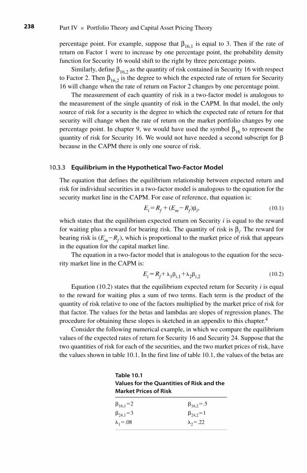
percentage point. For example, suppose that β16,1 is equal to 3. Then if the rate ofreturn on Factor 1 were to increase by one percentage point, the probability densityfunction for Security 16 would shift to the right by three percentage points.

Similarly, define β16,2 as the quantity of risk contained in Security 16 with respectto Factor 2. Then β16,2 is the degree to which the expected rate of return for Security16 will change when the rate of return on Factor 2 changes by one percentage point.

The measurement of each quantity of risk in a two-factor model is analogous tothe measurement of the single quantity of risk in the CAPM. In that model, the onlysource of risk for a security is the degree to which the expected rate of return for thatsecurity will change when the rate of return on the market portfolio changes by onepercentage point. In chapter 9, we would have used the symbol β16 to represent thequantity of risk for Security 16. We would not have needed a second subscript for �because in the CAPM there is only one source of risk.

10.3.3 Equilibrium in the Hypothetical Two-Factor Model

The equation that defines the equilibrium relationship between expected return andrisk for individual securities in a two-factor model is analogous to the equation for thesecurity market line in the CAPM. For ease of reference, that equation is:

Ei�Rf �(Em�Rf )�i, (10.1)

which states that the equilibrium expected return on Security i is equal to the rewardfor waiting plus a reward for bearing risk. The quantity of risk is βi. The reward forbearing risk is (Em�Rf ), which is proportional to the market price of risk that appearsin the equation for the capital market line.

The equation in a two-factor model that is analogous to the equation for the secu-rity market line in the CAPM is:

Ei �Rf��1�i,1��2�i,2 (10.2)

Equation (10.2) states that the equilibrium expected return for Security i is equalto the reward for waiting plus a sum of two terms. Each term is the product of thequantity of risk relative to one of the factors multiplied by the market price of risk forthat factor. The values for the betas and lambdas are slopes of regression planes. Theprocedure for obtaining these slopes is sketched in an appendix to this chapter.4

Consider the following numerical example, in which we compare the equilibriumvalues of the expected rates of return for Security 16 and Security 24. Suppose that thetwo quantities of risk for each of the securities, and the two market prices of risk, havethe values shown in table 10.1. In the first line of table 10.1, the values of the betas are


Table 10.1Values for the Quantities of Risk and theMarket Prices of Risk

�16,1�2 �16,2�.5

�24,1�3 �24,2�1

�1�.08 �2�.22

the quantities of risk contained in Security 16. Recall that Factor 1 is an equallyweighted portfolio of common stocks issued by the 10 largest firms in the transportationsector of the economy. The quantity of risk in a particular security with respect to thisfactor is the sensitivity of the expected rate of return on that security to changes in theaverage rates of return for these firms. The value of 2 for β16,1 means that the expectedrate of return for Security 16 will increase by two percentage points whenever the aver-age rate of return on the transportation sector increases by one percentage point.

Factor 2 is an equally weighted portfolio of common stocks issued by the 10largest firms in the financial services sector. The value of .5 for value for β16,2 meansthat the expected rate of return for Security 16 will change by one-half of one percent-age point (in the same direction) for each one percentage point change in the averagerate of return for the 10 largest firms in the financial services sector.

The second line in table 10.1 shows the values for two quantities of risk forSecurity 24. The value of 3 for β24,1 indicates that the expected rate of return forSecurity 24 will change by three percentage points in the same direction for eachchange of one percentage point in the average rate of return for the transportation sec-tor. Similarly, the value of 1 for β24,2 indicates that the expected rate of return forSecurity 24 will change by one percentage point for each change of one percentagepoint in the average rate of return for the financial services sector.

The values for the lamdas in the third line of table 10.1 are the values for the twomarket prices of risk. The easiest way to interpret these values is to compare theadjustments for risk between securities 16 and 24.

Each security has two quantities of risk, one for each factor. The market rewardsinvestors for bearing risk in a particular security by adjusting the expected rate ofreturn for that security. For each security, the size of the adjustment for the risk gener-ated by a specific factor depends on the quantity of that type of risk contained in thatsecurity, and on the market price for that type of risk. The market price of risk for agiven factor is the value of the lambda for that factor. As a market price of risk, thefunction of a lambda is to convert a quantity of risk into an adjustment in the expectedrate of return. For example, the value of .08 for λ1 means that for each percentagepoint of risk generated in a security by Factor 1, the market will increase the expectedrate of return on that security by .08 percentage points. Similarly, the value of .22 forλ2 means that for each percentage point of risk generated in a security by Factor 2, themarket will increase the expected rate of return on that security by .22 percentagepoints.

In table 10.1, the values for λ1 and λ2 are different because (for some reason)investors regard risk generated by Factor 2 as more burdensome than risk generatedby Factor 1. We cannot say anything more definite than this without a more sophisti-cated model. But the following observation is pertinent. In most asset pricing models,we assume that individual investors are perfect competitors. Consequently, eachinvestor must take the values of the parameters as fixed. But it is the competitionamong investors, as they trade securities to form their portfolios, that determines thevalues for the parameters. For example, the expected rate of return on Security 16 isthe standard deviation of that rate of return and the correlation coefficients betweenthe rate of return on Security 16 and the rates of return on all other securities depend-ing on the relative prices of all securities. Competition among investors determines


the relative prices of securities. Therefore, competition among investors determinesthe values of the parameters of the probability density functions that generate the ratesof return on these securities. An equilibrium is established when competition amonginvestors sets the values of the expected rates of return, the standard deviations, andthe correlation coefficients so that the Security Market Line in equation (10.2) issatisfied for each security.

Since the values for the betas and the lambdas are the slopes of regression linesthat involve rates of return, it is competition among investors that determines the val-ues of the betas and the lambdas. Consequently, if the value for λ2 exceeds the valuefor λ1, we infer that investors regard the risk generated by the sensitivity of a secu-rity’s rate of return to fluctuations in the rate of return on Factor 2 as more burden-some than the risk generated by Factor 1.

We will now use the values for the parameters in table 10.1 to calculate theexpected returns for Securities 16 and 24. Assume that the rate of return on thegovernment bond is .04. Then using the rate of return on the government bond, the values for the two lambdas in table 10.1, and the values for the two betas forSecurity 16 from table 10.1, and equation (10.2), we have:

(10.3)

The preceding equation states the risk-adjusted equilibrium expected rate ofreturn for Security 16 is 31% (per year). Four percentage points of this rate of returnare the reward for waiting; the remaining 27 percentage points are an adjustment forbearing risk. Also, 16 percentage points of the adjustment for risk are attributable tothe sensitivity of the rate of return on Security 16 to unpredictable variations in therate of return on Factor 1. The remaining 11 percentage points compensate for the sen-sitivity of the rate of return on Security 16 to unpredictable variations in the rate ofreturn on Factor 2.

Similarly, the equilibrium expected rate of return on Security 24 is:

(10.4)

The risk-adjusted equilibrium expected rate of return for Security 24 is 50% (per year). As in the case of Security 16, four percentage points of this rate of returnare the reward for waiting. The adjustment for bearing risk by holding Security 24 isequal to 46 percentage points, of which 24 are attributable to risk generated by Factor1, and 22 are attributable to risk generated by Factor 2.

We can increase our understanding of the two-factor model by comparing theadjustments for risk for Securities 16 and 24 in equations (10.3) and (10.4). Considerthe difference in the adjustments to the expected rates of return on the two securitiesfor the sensitivities of those securities to Factor 1. Security 16 has an adjustment of 16 percentage points for sensitivity to Factor 1, while the adjustment for Security 24for Factor 1 is 24 percentage points. This is because Security 16 has only two-thirds ofthe sensitivity to Factor 1 that Security 24 has to that factor. Both the probability

E24 .04 (.08)(3) (.22)(1)

.04 .24 .22

.50.

� � �

� � �

�

E16 .04 (.08)(2) (.22)(.5)

.04 .16 .11

.31.

� � �

� � �

�


density function for Security 16 and the probability density function for Security 24will shift when the rate of return on Factor 1 changes. Since β16,1�2 and β24,1�3, thedensity function for Security 16 will shift only two-thirds as far as the density functionfor Security 24 will shift. Consequently, the adjustment to the expected return forSecurity 16 is only two-thirds of the adjustment to the expected return for Security 24.

The market prices of risk are also important in determining the adjustments forrisk. We can see this by examining the set of values in table 10.1. From the second linein that table, we see that the quantities of risk contained in Security 24 are equal tothree for Factor 1 and one for Factor 2. This means that the probability density func-tion for Security 24 is three times as sensitive to changes in the rate of return on Factor1 as it is to changes in the rate of return on Factor 2. But the adjustment for risk attrib-utable to Factor 1 is not three times the adjustment for risk attributable to Factor 2. In fact, the adjustment for Factor 1 is 24 percentage points and the adjustment forFactor 2 is 22 percentage points. The reason is the difference in the values of the twomarket prices of risk. The price of a unit of risk based on Factor 1 is only .08; the priceof a unit of risk based on Factor 2 is .22. The price of risk for a factor is the number ofpercentage points by which the equilibrium expected rate of return on a security willincrease for each percentage point by which the expected value (or center point) of thesecurity’s probability density function shifts. The security’s density function shiftswhen the rate of return on a factor shifts.

10.4 The Three-Factor Model of Fama and French

Although early empirical tests of the CAPM were encouraging, subsequent and moresophisticated tests revealed anomalies. Perhaps the most celebrated of these anomaliesis the size factor, according to which investments in portfolios of small firms outper-formed the market, after allowing for risk. The combinations of expected rate of returnand beta for portfolios in general were scattered randomly above and below, but closeto, the security market line of the CAPM. But the combinations of expected rate ofreturn and beta for portfolios that were restricted to small firms plotted above thesecurity market line more frequently than could be attributed to chance. The implica-tion of this anomaly was that either the market consistently underprices the securitiesof small firms, or that the CAPM is not correct as a model of the equilibrium relation-ship between expected rate of return and risk.

Fama and French addressed this and other anomalies by augmenting the CAPM toinclude two factors in addition to the market factor. One of the new factors adjusts theequilibrium expected rate of return for a firm based on the size of the firm. The secondfactor is an adjustment based on the ratio between the book value of the firm and themarket value of its common stock. We consider the new factors in the next two sections.

10.4.1 The Factor for Size

The combinations of expected rate of return and beta for small firms are located abovethe security market line of the CAPM more frequently than chance would suggest.Therefore, according to the CAPM, the securities of small firms are underpriced; the


expected rate of return on a small firm is too high given the level of its risk as meas-ured by beta. The existence of excessive expected rates of return for small firms sug-gests that there are some aspects of risk in small firms that are not reflected in the valuesof the betas for those firms. Under this hypothesis, the CAPM does not set the prices ofsmall firms too low relative to the levels of risk in those firms. Rather, the CAPM under-states the levels of risk in small firms by using only beta to measure that risk.

To allow for the effect of the size of a firm on its equilibrium expected rate ofreturn, Fama and French proposed a size factor. Recall that a factor is a portfolio.Fama and French measure the size of a firm by the market value of its equity, that is,the price of a share of the firm’s common stock multiplied by the number of sharesoutstanding. The authors then rank firms according to size and form two portfolios.Portfolio S contains those firms that rank in the bottom half of all firms ranked bysize; Portfolio L contains the firms in the top half. For each month t, the rate of returnfor the size factor is defined as the rate of return on Portfolio S minus the rate of returnon Portfolio L.

To interpret the size factor, consider the following hypothesis. Suppose that theearnings of a small firm are more sensitive to unpredictable changes in interest ratesthan the earnings of large firms. Since it is difficult to predict the course of interestrates, investors who hold the securities of a small firm bear more risk (of unpre-dictable fluctuation in the rate of return on their portfolio) than they would if theyavoided those securities. Then to induce investors to hold the securities of small firms,the market must provide a higher expected rate of return on the securities of smallfirms. For a specific firm, the quantity of risk due to the size effect is the sensitivity ofthe rate of return of that firm to changes in the rate of return on the size factor. We willpursue this interpretation further in section 10.4.3, where we discuss the security mar-ket plane for the three-factor model.

10.4.2 The Factor for the Ratio of Book Equity to Market Equity

The second additional factor proposed by Fama and French depends on the ratio ofbook equity to market equity of a firm. The book equity of a firm is (approximately)the amount of money that the firm could raise by selling all its assets, minus the firm’sindebtedness to its contractual claimants. For example, if the firm has both bonds andcommon stock outstanding, the book value of equity would be the amount of moneythat the firm could pay to its shareholders after liquidating its assets and paying off thebondholders.

The market value of equity is simply the market price of a share multiplied by thenumber of shares outstanding. The book value of the entirety of a firm’s assets is theamount of money for which the firm could sell those assets. The prices that the assetswould bring in the market reflect the consensus of investors about the ability of thoseassets to generate earnings in alternative employment. Therefore, the book value ofthe firm’s assets is the opportunity cost of those assets. Consider, for example, a railroad that owns (rather than leases) its cars. The book value of those cars is theirvalue, as perceived by investors, of their most valuable alternative use. If other rail-roads have profitable opportunities to use additional cars, the book value of the cars


will be high. But if there is a surplus of cars among railroads, the book value of thecars will be low.

The market value of the railroad’s common stock is the greater of (1) the (risk-adjusted) present value of the earnings that the railroad’s current management cangenerate with the railroad’s assets, or (2) the book value of the railroad’s assets.Therefore, the market value of the railroad’s common stock is equal to the book valueof its assets plus whatever net value the management can add by using those assetsprofitably. Of course, profit must be calculated net of opportunity costs, and one ofthose opportunity costs is the book value of the equity. If the management is incompe-tent (or dishonest), the market value of the common stock could be less than the bookvalue of equity. In this case, the shareholders could increase their wealth by replacingthe current managers, because the most profitable use of the railroad’s assets is theircurrent use, given competent managers.

Alternatively, suppose that the managers are competent but that shippers andpassengers switch to other modes of transportation. Once again, the market value ofequity could be less than the book value of that equity. But in this case, the sharehold-ers would increase their wealth by liquidating the firm.

Either of the two examples described above could lead to a corporate takeover ofthe railroad. If the current shareholders are unable or unwilling to fire the current man-agers or liquidate the firm, a new set of investors could obtain a profit equal to the dif-ference between the book value and the market value of equity. The new investorscould purchase the railroad’s common shares at their market value, then use their newauthority as owners of the railroad either to replace the managers or liquidate the firm.

The market value of a firm’s equity depends on the price of the firm’s commonstock. Therefore, the market value of equity reflects investors’ beliefs about the ability of that firm to generate earnings. The book value of a firm’s equity is moredifficult to measure because, unlike the firm’s shares of common stock, the firm’sassets are not being continually priced on an organized exchange. Nevertheless, theratio of the two values of equity has empirical significance for asset pricing modelsand for other uses.

Define the book value of equity as BE, and the market value of equity as ME.Fama and French argue that a firm that has a high BE/ME ratio is a firm that investorsexpect to have relatively low (or slowly growing) earnings in the future. If investorsexpect future earnings to be low, they will be willing to purchase or hold the firm’sstock only at low prices. The low prices will create a low market value of equity, andhence a high BE/ME ratio. Similarly, investors will bid up the price of the stock of afirm that they expect will produce large earnings. The high price of the firm’s stockwill create a low BE/ME ratio for that firm.

Fama and French create a BE/ME factor as follows. First, the authors calculatethe BE/ME ratios for each firm over some historical period. They then rank the firmsby their historical BE/ME ratios. Next, they create two portfolios. The first portfoliocontains the firms in the upper half of the list of BE/ME ratios. The second portfoliocontains the firms in the lower half of the list. The value of the BE/ME factor formonth t is equal to the average rate of return over firms in the first portfolio for thatmonth, minus the average rate of return over firms in the second portfolio for thatsame month.


10.4.3 The Security Market Plane for the Three-Factor Model

Define the following:

Rm,t�Rf,t� the rate of return on the market portfolio minus the rate of return onthe risk-free asset, both for month t

RSize,t� the average of the rates of return on small firms minus the average of therates of return on large firms, for month t

RB/M,t� the average of the rates of return on firms with BE/ME ratios in thelower half of the list of all firms, minus the average of the rates of return onfirms with BE/ME ratios in the upper half of the list, for month t.

Let Ri be the rate of return on Security i. Then the three quantities of risk forSecurity i are:

(10.5)

The beta values are the slopes of the plane obtained by regressing the rate ofreturn on Security i against the rates of return on the three factors. Therefore, eachbeta value is the marginal effect of a factor on the conditional expected rate of returnof Security i.5

Finally, let the three market prices of risk be λM for the market factor, λSize for thesize factor, and λB/M for the BE/ME factor. The values for the lambdas are the slopesof the plane obtained by regressing the expected rates of return of all the securitiesagainst the beta values for those securities.

The three-factor model of Fama and French asserts that the equilibrium relation-ship between expected rate of return and risk is:

(10.6)

Equation (10.6) for the three-factor model of Fama and French is analogous toequation (10.2) in section 10.2 for the security market plane for our hypothetical two-factor model. The constant term is an estimate of the reward for waiting. Each termthat is a product of a lambda and a beta is an adjustment for risk.

10.4.4 The Size Factor and the Book-to-Market Factor as Predictors of Earnings

The rationale for including the market factor in the CAPM is clear. The market factorarises naturally in that model as a logical consequence of rational investors using theprinciples of portfolio theory to allocate their funds among risky securities. We wouldlike to have similar rationales for the size factor and the book-to-market factor thatFama and French include in their three-factor model. The fact that the three-factormodel has a good empirical record is welcome. We can have even more confidence inthat model because Fama and French provide a strong economic rationale for the inclu-sion of these factors as determinants of the expected rates of return on stocks. Thatrationale is that the two factors are predictors of a firm’s earnings. Since expected

Ei i i i� � � �Constant .M ,M Size ,Size B/M ,B/Mλ β λ β λ β

β σ

β σ

β

i M i M M

i i

i

R R

R R

,2

,Size Size size2

,B/M

Cov( , )/ ;

Cov( , )/ ;

Co

�

�

� vv( , )/ .B/M B/M2R Ri σ


rates of return depend on investors’ beliefs about the firm’s future earnings, it is logi-cal that investors would pay attention to any variables that have some power to predictfuture earnings.

10.5 The Five-Factor Model of Fama and French

10.5.1 An Integrated Market for Stocks and Bonds

Fama and French augmented their three-factor model by adding two factors to explainthe expected rates of return on bonds. The augmented model has a total of five factors.The five-factor model explains the equilibrium relationship between expected rate ofreturn and risk for both stocks and bonds with a single equation. The rationale for thisequation is that, although stocks and bonds are different kinds of assets, both stocksand bonds are risky securities.6 The rates of return on these securities are governed byprobability density functions. Therefore, we ought to be able to explain the relation-ship between the expected rate of return and the risk on these securities with a singleequation.

A good economic model will define a general principle that applies to a class ofphenomena. Any particular item in that class of phenomena conforms to the generalprinciple as a special case. Consider, for example, the common stocks of IBM and theUnion Pacific Railroad. These two firms are quite different, but there is a unifyingcharacteristic. An investor who holds a share of the stock of either firm owns asaleable right to receive an uncertain sequence of payments. The expected rate ofreturn on each security depends on investors’ beliefs about the probability densityfunction that governs that firm’s earnings. Obviously, it would be unsatisfactory tohave one asset pricing model to explain the expected rate of return and risk for IBM,and a separate model to explain the expected rate of return for the Union PacificRailroad. Nor do we want one asset pricing model for firms whose business is trans-portation and a different model for firms in the computer industry. We want a singlemodel that is sufficiently general to accommodate both types of firm.

The same reasoning applies to stocks and bonds. Both are financial securitieswhose rates of return are governed by probability density functions. We want a singlemodel that will explain the equilibrium relationship between expected rate of returnand risk for both kinds of securities.

10.5.2 The Factor for the Term Structure of Interest Rates

The first factor that Fama and French added to enable their model to explain theexpected rates of return on bonds is designed to recognize that one source of risk forbondholders is unexpected changes in the interest rates offered by alternative securi-ties. Interest rates are, of course, a form of opportunity costs. Fama and French calltheir proposed factor TERM, which they define as:

TERMt�rate of return on a long-term government bond for month t�rate of return on a one-month U.S. Treasury bill for month t.

The value of the factor TERMt is a proxy “for the deviation of long-term bondreturns from expected returns due to shifts in interest rates.”7


10.5.3 The Factor for the Risk of Default

The second factor proposed by Fama and French is designed to capture the riskthat the firm might fail to make the required payments on interest and principal ontime. Fama and French call this factor DEF because it is a proxy for the risk of default.The default factor is defined by:

DEFt � rate of return on a portfolio of long-term corporate bonds for month t�rate of return on a long-term U.S. government bond for month t.

Since no one expects the federal government to default on its bonds,8 changes inthe value of the DEF factor measure changes in the risk of default on corporate bonds.Specifically, an increase in the value of the DEF factor from month t to month t �1would occur if investors require a larger premium to hold bonds issued by corpora-tions rather than bonds issued by the government. A plausible reason for an increase inthe difference between the rates of return on the two kinds of bonds is that investorsexpect a higher probability of default on corporate bonds.

10.5.4 The Security Market Plane for the Five-Factor Model

Define the quantity of risk for Security i for the TERM factor as:

(10.7)

Then βi,TERM is the sensitivity of the rate of return on Security i to changes in thevalue of the TERM factor. That is, βi,TERM is the amount by which the conditionalprobability density function for Security i shifts when the value of the TERM factorincreases by one percentage point.

Similarly, the quantity of risk for Security i for the DEF factor is:

(10.8)

The five-factor model proposed by Fama and French for the equilibrium relation-ship between the expected rate of return and risk on both stocks and bonds is:

Ei � Constant � λMβi,M � λsizeβi,size� λB/M βi,B/M � λTERM βi,TERM

� λDEFβi,DEF, (10.9)

in which λTERM is the market price of risk for the TERM factor, and λDEF is the market price of risk for the DEF factor.

For any particular security, the values of one or more of the betas could be zero.For example, if Security i is a common stock for which the risk of default on corporatebonds has no bearing, the value of βi,DEF will be zero.

10.6 The Arbitrage Pricing Theory

10.6.1 A Brief Statement

The APT is a special case of a multifactor model. The distinguishing feature of theAPT is that the factors are generated endogenously by an empirical technique called

β σi ir r,DEF DEF DEF2Cov( , )/ .�

β σi ir r,TERM TERM TERM2Cov( , )/ .�


factor analysis. As is the case with any multifactor model, each factor is a portfolio ofsecurities. But these portfolios, or factors, are not chosen by the investigator on thebasis of inferences drawn from economic theory or from previous empirical studies.Rather, factor analysis chooses the factors based on the ability of the resulting modelto explain differences in the expected rates of return on individual securities by usingdifferences in the securities’ quantities of risk with respect to the factors. Following isa brief summary of how a model based on the APT is constructed.

Factor analysis is an empirical procedure that generates a sequence of iterations.Keep in mind that a factor in an asset pricing model is a portfolio of securities. Eachiteration of the factor analysis produces a set of factors to define a specific multifactormodel of the relationship between the quantities of risk and expected rates of returnfor individual securities. Each multifactor model is then tested to determine howclosely its predictions fit the data. Based on the results of the test for closeness of fit,the next iteration produces a revised set of factors, and hence a revised multifactormodel. The process continues until it produces a model that satisfies a threshold forcloseness of fit chosen by the investigator.

Here is an example of how the technique of factor analysis works. An investiga-tor begins with historical data on the rates of return for a large set of securities. Forexample, she might use data on every security in the S&P 500 for the past 20 years.Using these data, the investigator uses factor analysis to construct an initial set of port-folios to use as factors. The composition of these initial portfolios need not detain us.For the purpose of example, suppose that there are four factors. Factor 1 might be aportfolio in which 20% of the investment is allocated to IBM, 70% to GE, and 10% toUnion Pacific Railroad. Factor 2 could be a portfolio in which funds are distributedequally over the five largest airlines in the economy. Factor 3 might be a portfolio inwhich funds are distributed over the largest 20 firms that have an unbroken record ofpaying dividends over the last 10 years. In this portfolio, the funds are allocated acrossthe 20 firms in proportion to the relative market values of those firms’ outstandingcommon stock. Finally, Factor 4 might require an investment in 20 firms that have nodiscernible property in common. A distinguishing property of factor analysis is thatthe empirical procedure is free to define the factors in any way that produces a modelthat, for whatever reason, satisfies a threshold for closeness of fit.

Once the portfolios (factors) are chosen for a given iteration of the procedure, thenext step is to calculate the quantities of risk for each security for each of the factors.These quantities of risk have the same interpretation as the quantities of risk in themultifactor models examined earlier in this chapter.

Next, the procedure calculates the market prices of risk for each factor. Again, asin any multifactor model, these prices of risk are determined by regression, using acriterion of closeness of fit.

Finally, using the quantities of risk for each security for each factor, and the mar-ket prices of risk for each factor, the resulting multifactor model is tested for its abilityto predict the relationships between expected rates of return and quantities of risk foreach security. A measure of closeness of fit is obtained. Based on this measure, thefactor analysis generates a revised set of factors, and thus a revised factor model, sub-ject to the condition that the revised model will produce a closer fit between expectedrates of return and quantities of risk.


In some applications of factor analysis, the investigator chooses the number offactors that the empirical procedure may select; in other applications, the empiricalprocedure is free to vary the number of factors. But in any case, the objective is to pro-duce a multifactor model that will explain the observed relationship across securitiesbetween expected rates of return and quantities of risk.

10.6.2 A Simple Comparison of an Arbitrage Pricing Model and a Factor Pricing Model

The following equation is an example of an arbitrage pricing model that has fourfactors:

(10.10)

A comparison of equation (10.10) with equation (10.9) shows that the structure ofan arbitrage pricing model (with four factors) is identical to that of any specific multi-factor asset pricing model that also has four factors. Each model states that the equi-librium expected rate of return on Security i is equal to a constant (which could be thereward for waiting) plus four adjustments for risk. In each model, each adjustment forrisk is the product of two terms; those terms are a quantity of risk and the market priceof that type of risk. Each quantity of risk is a covariance between the rate of return onSecurity i and the rate of return on a specific portfolio. The difference between the twomodels is that the four types of risks in the model of equation (10.9) are specified inadvance by the researcher, whereas in the arbitrage pricing model of equation (10.10),the four types of risk are determined within the model (endogenously) by an algorithmthat maximizes the closeness of fit.

10.6.3 Additional Observations about Arbitrage Pricing Models

A disadvantage of factor analysis is that the portfolios that are generated for thefactors can be difficult to interpret. It is unlikely, for example, that any of the factorsthat will emerge from an application of factor analysis will contain securities with thekinds of common properties that we see in Factors 1, 2, and 3 in our example above.More likely, each factor will be like Factor 4, in which the constituent securities do nothave any obvious property in common. It is then not clear what the quantities of risk,or the market prices of risk, in the model mean. One can say that the model works inthe sense of producing a certain closeness of fit. But one cannot easily provide an intu-itive rationale for why the model works, as one can with the three-factor model andthe five-factor model of Fama and French.

Finally, a word about the term arbitrage in the arbitrage pricing model.9 Mostmodels of equilibrium in financial economics (and in several other areas of economicsas well) rely on the process of arbitrage to enforce the predicted equilibrium relation-ship between prices and quantities. We have seen this in the derivation of the securitymarket line in the capital asset pricing model in chapter 9. If the values of the param-eters for Security i and the market portfolio enable an investor to construct a portfoliothat lies above the capital market line, then competition among investors (acting asspeculators) to exploit this opportunity will cause the price of Security i to change.

Ei i i i� � � � �Constant 1 ,Factor 1 2 ,Factor 2 3 ,Factor 3 Facλ β λ β λ β λ ttor 4 ,Factor 4βi


As the price of Security i changes, the values of the parameters of that security willchange so as to eliminate the opportunity to use Security i to create a portfolio that liesabove the capital market line. The same reliance on arbitrage occurs both in the multi-factor models studied earlier in this chapter and in the arbitrage pricing model.Arbitrage, as part of the rationale for explaining why a model works, is not limited tothe arbitrage pricing model.

10.7 Summary

The fundamental contribution of the CAPM is that the quantity of risk in a security isproportional to the covariance between the rate of return on that security and the rateof return on a special portfolio. We know that, for the CAPM, the special portfolio isthe market portfolio. Unfortunately, the empirical record of the CAPM is not satisfac-tory. Among the several anomalies is the size effect, according to which the market(that is, investors) systematically underprices the securities of small firms.

Fama and French address the empirical shortcomings of the CAPM by presentingtwo models. Each model augments the CAPM by adding factors. In addition to themarket factor from the CAPM, the three-factor model has a factor for size and a factorfor the BE/ME ratio. For Security i, the quantity of risk associated with the size factoris the covariance between the rate of return on Security i and the difference between therates of return on a portfolio of small firms and a portfolio of large firms. Similarly, thequantity of risk for the book-to-market factor is the covariance between the rate ofreturn on Security i and the difference between the rates of return on a portfolio of firmsthat have high BE/ME ratios and a portfolio of firms that have small BE/ME ratios.Each factor has its own market price of risk. Fama and French demonstrate (empiri-cally) that the size and book-to-market factors are proxies for future earnings, whichprovides an economic rationale for augmenting the CAPM by these factors.

Since both stocks and bonds are risky securities, and since investors can use themarkets for both securities in constructing their portfolios, we should be able toexplain the expected rates of return on both stocks and bonds with a single equation.To do this, Fama and French add to their three-factor model two factors to recognizethe sources of risk that apply particularly to bonds. One of these factors captures therisk of default; the second factor is a proxy for the risk of unexpected changes in inter-est rates. The resulting five-factor model has a good empirical record.

The central contribution of the CAPM survives in the models of Fama andFrench. The risk of a security is measured by one or more covariances between therate of return on that security and the rates of return on one or more portfolios.

Appendix: Estimating the Values of � and � for a Two-Factor Model

Let there be N risky securities indexed by i �1, . . . , N. In a two-factor model, theequilibrium expected rate of return for Security i is:

Ei �Rf �λ1βi,1�λ2βi,2, (10.11)


in which Ei is the expected rate of return on Security i, Rf is the rate of return on therisk-free asset, λ1 and λ2 are the market prices of risk associated with Factors 1 and 2,and βi,1 and βi,2 are the quantities of risk associated with Factors 1 and 2 for Security i. To use equation (10.11), we need values of βi,1 and βi,2 for each of the Nsecurities. We also need values for λ1 and λ2.

We use a two-stage multivariable regression to estimate the values of the twolambdas and the 2N betas. We estimate the values of the betas first.

For each Security i, we estimate the values of βi,1 and βi,2 by regressing the rate ofreturn for Security i on the rates of return of the two factors for some historical period.The estimated values for βi,1 and βi,2 are the slopes of the (three-dimensional) regres-sion plane in the dimensions that represent the two factors.

Suppose that we are using monthly rates of return over a period of five years.Then for each month we have a three-dimensional data point. To visualize the three-dimensional regression, draw one axis across this page from left to right. Draw a second axis from the bottom of the page to the top. Make the two axes perpendicularto each other. Finally, draw a third axis perpendicular to the plane of the page andpassing through the intersection of the first two axes. We measure the rate of return ofFactor 1 on the first axis, the rate of return of Factor 2 on the second axis, and the rateof return on Security i on the third axis. Then for each month the rates of return of thetwo factors and the rate of return on Security i are the coordinates of a point located inthe three-dimensional space that contains the plane of the page. Suppose that in agiven month the rate of return of Factor 1 is positive, the rate of return of Factor 2 isnegative, and the rate of return of Security i is positive. Then the three-dimensionalpoint for that month will lie to the right of the second axis (that runs from the bottomof the page to the top), below the first axis (that runs from left to right across thepage), and above the plane of the page. Since we are using monthly data over a periodof five years, we will have 60 data points in the three-dimensional space that containsthis page.

To regress the rate of return of Security i on the rates of return of the two factors,we fit a plane to the set of 60 data points. As in ordinary regression, we choose the plane that minimizes the sum of the squared distances from the data points to theregression plane. If we were to regress the values for a variable y on a variable x, wewould fit a straight line to a set of two-dimensional data points. We would choose the intercept and the slope of that line to minimize the sum of squared vertical dis-tances from the data points to the line.

We can define a straight line by specifying the value of its intercept with one axis(usually the vertical axis) and the value of its slope with respect to the other axis (usu-ally the horizontal axis). Analogously, we can define a plane by specifying the valueof its intercept with one of the three axes and the values of its slopes with respect tothe other two axes. In the regression for Security i against the two factors, the value ofβi,1 is the slope of the plane with respect to the axis that runs across the page from leftto right. The value of βi,2 is the slope of the plane with respect to the axis that runsfrom the bottom of the page to the top.

To interpret these slopes as quantities of risk, consider a typical data point. Thecoordinates of this point for the two factors locate the point on the page; the coordi-nate for the rate of return of Security i determines the height of the data point above


this page. This height above the page is the expected rate of return on Security i con-ditional on the rates of return on the two factors.

Suppose that the rates of return of Factors 1 and 2 are F1 and F2. Let these rates ofreturn be the coordinates of Point H on the plane of this page. Then the height of theregression plane over Point H is the conditional expected rate of return for Security i,if the rate of return of Factor 1 is F1 and the rate of return of Factor 2 is F2. Supposethat the rate of return of Factor 1 increases by one percentage point, while the rate ofreturn of Factor 2 does not change. Let Point J on the plane of this page represent thenew coordinates. Then Point J will lie horizontally to the right of Point H by .01. Thedifference in the heights of the regression plane over Points H and J is the marginaleffect of Factor 1 on the conditional expected rate of return of Security i. Therefore,the slope of the regression plane with respect to Factor 1, which is the value of βi,1, isthe marginal effect of Factor 1 on the conditional expected rate of return of Security i.Similarly, the value of βi,1 is the marginal effect of Factor 2 on the conditionalexpected rate of return of Security i.10

To estimate the values of the lambdas, which are the market prices of risk, we needone final regression. In the CAPM there is a single source of risk, namely the volatilityof the rate of return on the market portfolio. Consequently, there is a single marketprice of risk that applies to all securities. In a two-factor model, the two sources of riskare the volatilities of the rates of return with respect to changes in the values of the twofactors. Consequently, there are two market prices of risk that apply to all securities.These market prices of risk are λ1 for Factor 1 and λ2 for Factor 2. To estimate the val-ues of the two lambdas, we regress the values of the historical average rates of return onthe N securities against the N pairs of values of betas for those securities.

Let the axis that runs across this page from left to right represent Factor 1, the axisthat runs from the bottom of this page to the top represent Factor 2, and the axis that isperpendicular to the page represent the historical average rate of return on a security.For this regression, we have N data points, one for each security. The coordinates ofthe data point for Security i are (βi,1, βi,2, Ei). We plot the first coordinate on the axisthat runs across the page, the second coordinate on the axis that runs from the bottomto the top of the page, and the third coordinate on the axis that is perpendicular to thepage. We then fit a plane to the N data points. The slope of the plane in the dimensioncorresponding to Factor 1 is the value of λ1, and the slope of the plane in the dimen-sion corresponding to Factor 2 is the value of λ2.

Note that each security has its own values for the two betas. Therefore, toestimate the values for the betas we need N regressions, one for each security. Butthere is only one pair of values for the market prices of risk. Therefore, we need onlyone regression to estimate the values of the lambdas.

Problem

Consider the following numerical example in which we compare the equilibrium val-ues of the expected rates of return for Security 19 and Security 84 in a two-factormodel:


The two quantities of risk for each of the securities, and the two market prices ofrisk, have the following values:

β19,1�5 β19,2�.8

β84,1�7 β84,2�3

λ1�.11 λ2�.25

(a) Interpret each of the values.(b) Assume that the rate of return on the government bond is .10. Using this

value, the values for the two lambdas, and the values for the two betas forSecurity 19 and Security 84, calculate the risk-adjusted equilibrium expectedrates of return for Security 19 and Security 84.

Notes

1. The postulates are axiomatic assertions about properties of any person’s choices. Thesepostulates include: more of any Good X is better than less of that good, given no changes in thequantities of any other good; willingness to forego some amount of any Good Y (per unit oftime) in order to gain an additional unit of another Good X (willingness to substitute betweenGoods X and Y); and willingness to substitute between Goods X and Y at a diminishing marginal rate (the larger the quantity of Good X that a person has, the smaller the quantity ofGood Y he is willing to forego to obtain one additional unit of Good X). For the derivation ofthe CAPM, the context includes assertions such as the rates of return on (almost) any two secu-rities are imperfectly correlated.

2. In fact (as we know) the measure of risk for a security is proportional to the covariancebecause the beta for a security is equal to the covariance between the rate of return on that secu-rity and the rate of return on the market portfolio, with that covariance divided by the varianceof the rate of return on the market portfolio.

3. For an excellent discussion and application of the choice of factors for a multifactor model,see N. R. Chen, R. Roll, and S. Ross, “Economic Forces and the Stock Market,” Journal ofBusiness 59, no. 3 (1986): 383–403; E. Fama and K. French, “Common Risk Factors in theReturns on Stocks and Bonds,” Journal of Financial Economics (February 1993): 3–56.

4. Let y and x be variables. The regression of y on x will produce a straight line of the formy��βx, in which y is the estimated (or predicted) value for y given the value for x. The termsα and β are parameters whose values are determined by minimizing the sum of squared differ-ences between the actual and the predicted values for y given the values for x. The slope of theregression line is β, whose value is the increase in the predicted value for y given an increase ofone unit in the value for x. If we were to regress the variable y on the two variables x and w, wewould obtain a plane defined by the equation y′�α′�β′x�γ ′w. The terms β′ and γ ′ are param-eters whose values are the slopes of the plane in the directions parallel to the axis on which thevalues for x and w are plotted. For example, the value for β′ is the increase in the predicted valuefor y given an increase of one unit in the value for x, holding the value of w constant.

5. The plane obtained by regressing rate of return on Security i on the three factors will be a (hyper)plane in four-dimensional space. We will not attempt to visualize this plane.Nevertheless, the interpretation of the betas as the marginal effects of factors on the conditionalexpected rate of return of Security i holds. The procedure is analogous to that described in note 4 for the hypothetical two-factor model.


6. Although a bond is a contractual claim on the firm’s earnings, the bond is a risky securitybecause the market price of the bond can change at any time prior to the maturity date. A changein the current price of the bond creates a capital gain or loss for the investor who holds thatbond. The rate of return on any security held from time t to time t�1 depends, in part, on thechange in the price of that security over that interval. The price of a bond can change for tworeasons. First, the firm might fail to make the required payments of interest and principal ontime. Changes in investors’ beliefs about the probability that the firm will not make the requiredpayments will change the current price of the bond. Second, the rates of interest offered by othersecurities, such as U.S. Treasury bonds or certificates of deposit at a bank, might change.Changes in the interest rates offered by alternative securities change the opportunity cost ofholding a firm’s bond, which will change the current price of the bond. Investors who purchasebonds are not committed to holding those bonds to their maturity any more than investors whopurchase stocks are committed to holding those stocks as long as the firm exists. In both cases,the typical investor is concerned about the capital gains and losses from period to period, aswell as payments of interest and dividends.

7. Fama and French, “Common Risk Factors in the Returns on Stocks and Bonds.” (Seecitation in Note 3.)

8. We must distinguish between a nominal default and a purchasing power default. A nomi-nal default would occur if the government failed to pay the amounts of money on the schedulepromised by the bond. No one expects a nominal default, so the bonds are riskless in this sense.The government might (through monetary policy) inflate the price level, which would reducethe purchasing power of the promised payments of money. Recently, the government hasoffered bonds whose payments are indexed to the price level. These bonds are fully risklessbecause investors are protected against both kinds of default.

9. Arbitrage is a process in which an investor obtains a risk-free profit, net of opportunitycosts, by simultaneously purchasing an underpriced security and selling an overpriced security.In many cases one or both securities are portfolios constructed by the investor. Sophisticatedexamples of arbitrage appear in chapter 15 on options.

10. Since we are estimating the values of βi,1 and βi,2 with linear multivariable regression, theresult of the regression is a plane. The two slopes of a plane are constants. Therefore, the estimated marginal effects of the two factors are constants.



Part V

The Informational andAllocative Efficiency ofFinancial Markets:The Concepts

11.1 Introduction

11.1.1 The Efficient Markets Hypothesis Defined

The efficient markets hypothesis is “the simple statement that security prices fullyreflect all available information.”1 Empirical tests of this hypothesis require a precisedefinition of the term fully reflect. A security is a saleable right to receive a sequenceof payments. Both the amounts and the timing of these payments can be uncertain.The price of a security fully reflects all available information about the sequence ofpayments associated with that security if the marginal profit that an investor couldearn by collecting additional information is zero.

The preceding definition of the term fully reflects has two implications that areimportant in discussions of the efficient markets hypothesis. The first implication isthat so long as the costs of collecting information are positive, there will be someinformation about sequences of future payments that is not reflected in the prices ofsecurities. The second implication is that to obtain a profit by collecting and trading oninformation, an investor must have a marginal cost for collecting information that islow relative to the marginal cost for a typical investor.

Consider the first implication. If the marginal cost of collecting and trading oninformation about future values of prices were zero, then competition among investorswould cause current prices to reflect this information. If this were not so, any investorcould obtain a profit by trading in the securities whose prices do not fully reflect theinformation. For example, consider the models in chapter 5, where we examined theeffect on the price of a firm’s stock when the firm announces a new project. In thatchapter, we assumed that all future payments are known with certainty today. We alsoignored transaction costs such as brokers’ commissions and the opportunity cost of aninvestor’s time. Then the marginal cost of collecting and acting on information is zero.Competition among investors causes the current prices of securities to reflect all infor-mation about future payments. In particular, prices will change to reflect immediatelyany new information, such as the announcement of a new project.

Instead of using the assumptions in chapter 5, suppose that investors must incurcosts to assess the accuracy of a firm’s announcement of a new project. Then the priceof the firm’s stock would reflect the information about the project only to the point atwhich the marginal profit of collecting more (or more accurate) information and trad-ing on it is equal to zero. As long as the marginal costs of collecting and trading on

11 The Efficient Markets Hypothesis

257

information are positive, there will be some information that is not reflected in theprices of securities.

In chapter 9, we defined the risk-adjusted residual on a security as that portion of thesecurity’s rate of return that cannot be attributed to the rewards for waiting and for bear-ing risk.2 In the CAPM, the residual is the vertical distance between the rate of return andthe characteristic line. The residuals should be random, which means that they should notbe predictable from one period to the next. There is, however, some evidence that theresiduals are, to a small degree, predictable. The predictability of residuals would be suf-ficient to invalidate the efficient markets hypothesis only if the marginal costs of collect-ing and trading on information were zero. Since these costs are not zero, a certain degreeof predictability of residuals is consistent with the efficient markets hypothesis.

This brings us to the second implication of our definition of the term fully reflectsin the statement of the efficient markets hypothesis. The efficient markets hypothesisstates that the prices of securities fully reflect all information about future sequencesof payments. If this hypothesis holds, then no investor can obtain a profit by collectinginformation and trading on it. But clearly some investors do obtain profits by identify-ing mispriced securities. The existence of these investors is taken by some persons asconclusive evidence that the efficient markets hypothesis is false. This conclusion isunwarranted. The existence of some investors who can identify mispriced securities iscompatible with the efficient markets hypothesis because investors differ in the mar-ginal costs that they incur to collect, analyze, and trade on information. Investors whohave a comparative advantage in identifying mispriced securities will specialize indoing so. The activities of these investors will cause prices to contain more informa-tion than they otherwise would. But so long as even these investors incur positivemarginal costs, the prices of securities will not fully reflect all information aboutsequences of future payments.

11.1.2 The Weak, the Semistrong, and the Strong Forms of the Efficient Markets Hypothesis

As first exposited in 1972 by Eugene Fama, the efficient markets hypothesis waspartitioned into three concatenated forms: the weak, the semistrong, and the strong.3

Each form was defined for a specific set of information.

The Weak Form

The weak form of the efficient markets hypothesis was limited to historical informationabout the prices of securities and the volumes at which those securities were traded.The weak form stated that the current prices of securities fully reflected all informationcontained in the history of the prices and the volumes of trading. Consequently, the netmarginal benefit to an investor of collecting information from past prices and volumesof trading for the purpose of predicting the future prices of securities is zero.

As an empirical fact, there is some serial correlation in the prices of securities.Therefore, there is some information in the past values of prices and volumes oftrading that is useful in predicting the future values of prices if an investor can collect

Part V ■ Informational and Allocative Efficiency: Concepts258

and analyze that information at a zero cost. But these costs are not zero for anyone,especially if one includes the opportunity costs incurred by spending time trying topredict the prices of securities rather than exploiting one’s comparative advantage inother pursuits. Those whose comparative advantage does lie in predicting the prices ofsecurities by examining data on past prices and volumes of trading should do so.These persons have lower marginal costs for predicting future prices from past datathan the rest of us do.4 In equilibrium, competition among these persons shouldimprove the extent to which current prices reflect the information contained in pastprices and volumes to the point at which the net marginal benefit for the rest of us fallsto zero or below.

The presence of statistically significant serial correlation in the prices of securi-ties is not equivalent to the presence of economically significant serial correlation,unless everyone can collect and analyze information, and trade on that information, atzero marginal costs. For most persons, the net marginal benefit of analyzing historicalinformation is zero or negative. Thus, for most of us the weak form of the efficientmarkets hypothesis holds, even in the presence of empirically detectable serial corre-lation among prices of securities.

The Semistrong Form

The semistrong form of the efficient markets hypothesis states that the current pricesof securities fully reflect all public information about the future values of those prices.Public information includes everything that one could learn from reading the publicpress and attending meetings that are open to the public. Since the public press reportshistorical information on prices and volumes of trading, the set of information for theweak form is contained within the set of information for the semistrong form.

The implication of the semistrong form of the hypothesis is analogous to theimplication of the weak form, namely that the marginal benefit of analyzing publicinformation in an attempt to predict the future prices of securities is zero. Once again,comparative advantages in analyzing public information differ across persons. And, as in the case of the weak form, we would expect that those persons whose mar-ginal costs are relatively low would specialize in analyzing public information to the extent that the net marginal benefit for the rest of us in doing so is zero or nega-tive. There is substantial empirical evidence that this is so. The ability of mutual fund managers consistently to outperform the market, after allowing for the levels ofrisk in their portfolios, and after subtracting the costs incurred to operate the mutualfunds (which costs include the salaries paid to their financial analysts), is (close to)zero.5

The Strong Form

Finally, economists include the strong form of the hypothesis for logical complete-ness. The strong form states that the current prices of securities fully reflect all infor-mation about the future values of those securities. The set of information for the strongform includes all private, as well as all public, information. For example, the minutes

Chapter 11 ■ The Efficient Markets Hypothesis 259

of boards of directors and the reports of biologists employed by pharmaceutical firmswould be part of the set of private information. No one believes that the efficientmarkets hypothesis holds in the strong form. Numerous empirical studies demonstrateconclusively that corporate insiders do possess material information about the futureprices of securities, and that these insiders do trade on that information.6

11.1.3 Random Walks and the Efficient Markets Hypothesis

There is often confusion between the efficient markets hypothesis and the hypothesisthat the prices of securities are governed by a random walk. A random walk is a partic-ular kind of stochastic process. A stochastic process is a process that generates asequence of values for some variable by taking draws from a sequence of probabilitydistributions. In the general case, the parameters of the probability distribution thatgenerates the value at time t depend on the values generated at times prior to time t.That is, the distribution that governs the process at any specific time depends on theevolution of the process up to that time. A random walk is a stochastic process inwhich the probability distribution that generates the outcomes does not depend on theevolution of the process. In the simplest case of a random walk, the probability distri-bution never changes throughout the process.7

There is considerable evidence that the changes in the prices of stocks follow arandom walk with a positive drift. The positive drift reflects the growth of the econ-omy over the longer term. In an efficient market, the current prices of securities fullyreflect all current information about the abilities of the issuing firms to generate earn-ings over the future. Hence, the current prices reflect all current information about thefuture values of those prices. Prices change over time because new informationbecomes available. New information, by definition, is unpredictable. Some informa-tion arrives at predictable times, such as a firm’s quarterly announcement of its earn-ings, but the information itself is unpredictable with certainty. Other information, suchas a decision by a federal court in an antitrust case, is unpredictable both in its timingand in its content. It is the unpredictability in the arrival and the content of informationthat causes the prices of securities to change unpredictably.8

Some persons misinterpret the term random walk to mean that the prices of secu-rities are random in the sense that there is no logical relationship between those pricesand the ability of the issuing firms to generate earnings. This is incorrect. There is adiscernible logic with which one can explain the prices of securities in terms of infor-mation about firms and the economy. This logic is defined by the various asset pricingmodels that we have studied. It is not the prices of securities that are random. Rather itis the sequence of changes in the prices that is random, because the arrival of informa-tion is random.

The efficient markets hypothesis states that once information arrives, the marketimmediately, and without bias, adjusts the prices of securities to reflect that informa-tion so as to eliminate opportunities for risk-free profits for speculators net of transac-tion costs. The efficient markets hypothesis makes no claim about the timing or thesignificance of new information. A random walk of changes in the prices of securitiesis consistent with the efficient markets hypothesis.9


11.1.4 The Significance of the Efficient Markets Hypothesis for Economic Efficiency

The efficient markets hypothesis also has a critical bearing on the question of the effi-cacy of financial markets in promoting an efficient allocation of resources. In anefficient allocation of resources, all opportunities for mutually beneficial exchanges arerealized. Put another way, in an efficient allocation there are no further opportunities toincrease the welfare of any person (or persons) without decreasing the welfare of someother person (or persons). To allocate resources efficiently, the economy must first iden-tify the potential mutually beneficial exchanges and then transmit information aboutthese opportunities to the persons who own the resources. A market economy uses pricesto transmit this information. Consequently, to achieve an efficient allocation of resourcesthe prices must fully reflect the benefits and the costs of all possible exchanges.

Financial markets promote intertemporal exchanges by facilitating the trading offinancial securities. In a typical intertemporal exchange, one person pays money now toacquire a financial security from a second person. The second person is often a group ofpersons acting through a firm, and the payments in the sequence are usually uncertain.

The price of the security is the risk-adjusted net present value of the associatedsequence of payments. The prices of securities must fully reflect these net presentvalues if the financial markets are to achieve an efficient allocation of resources.

We conclude that the efficient markets hypothesis is much more than an interest-ing empirical question. The hypothesis has implications for the regulation of financialmarkets. If the prices of securities do not fully reflect the information about sequencesof payments, there will be an inefficient allocation of resources. Alternatively, if thehypothesis is correct, so that security prices do fully reflect the relevant information,then regulation of financial markets could impede an efficient allocation of resources.

The efficient markets hypothesis is a claim about informational efficiency.Economic efficiency is a criterion by which we evaluate an allocation of resources.In a complex market economy, informational efficiency is a necessary condition foreconomic efficiency.

11.2 Informational Efficiency, Rationality, and the Joint Hypothesis

11.2.1 The Joint Hypothesis and the Equilibrium Values of Prices

The efficient markets hypothesis is one part of a joint hypothesis that involves (1) theclaim that security prices fully reflect all the information about the associated sequencesof payments, and (2) a claim that prices are equal to a particular set of equilibrium val-ues. To test the efficient markets hypothesis is to test jointly the claim that prices are attheir equilibrium values and the claim that we know what the equilibrium values are.

11.2.2 A Simple Example from Introductory Economics

Consider the following heuristic example. A perfectly competitive industry is in long-runequilibrium, and the long-run industry supply curve is upward sloping. The government


asks economists to predict the effect on the equilibrium price paid by consumers if atax were imposed on each firm equal to $4 for each unit produced and sold. The econ-omists predict that the equilibrium price to consumers would increase, but by less than$4, and that the elasticities of demand and supply would determine the size of theincrease. This prediction is an elementary application of the theory of the firm. Butthis theory is based on several assumptions, one of which is that firms attempt to max-imize profits. It is easy to show that (unless firms’ marginal cost curves are horizontal)a profit-maximizing firm will not attempt to pass on the full amount of the tax to con-sumers in the form of a higher price.10

Suppose that empirical tests of the economists’ predictions show that imposing aunit tax imposed on perfectly competitive firms causes the price to increase by the fullamount of the tax. We could interpret this empirical result in at least two ways. First,we could conclude that the tax does increase the long-run equilibrium value of theprice by less than the tax, but that the market inefficiently adjusts the price to its newequilibrium value. In particular, the market initially increases the price by the fullamount of the tax, and then adjusts the price downward toward its new equilibriumvalue only very slowly over time. That is, the price that appears immediately after thetax is imposed does not fully reflect the information that the new (long-run) equilib-rium price has increased by less than the amount of the tax.

The second possible interpretation is that firms do not attempt to maximize prof-its. For example, suppose that firms set prices by adding a certain markup to averagetotal cost. In this case, imposing on each firm a tax equal to $4 for each unit producedand sold does increase the equilibrium price by $4. Under this interpretation, when theprice increases by the full amount of the tax it does fully reflect the information aboutthe new equilibrium price. In this case, the market is informationally efficient; theeconomists used the wrong model to predict the effect of the tax on the equilibriumprice.

We conclude that any test of the effect of a tax on the equilibrium price in a com-petitive industry is necessarily a test of a joint hypothesis. A test of whether the priceincreases by less than the tax is simultaneously a test of the efficiency with which themarket transmits information through prices and a test of the assumptions that under-lie the economists’ model of the firm. If the price increases by the full amount of thetax, it is impossible to distinguish which of the two hypotheses failed. Alternatively,suppose that the empirical tests show that the price increases by less than the tax. Wecannot know whether the market is informationally efficient (because we have thecorrect model of the firm to predict the new equilibrium price) or whether the marketis inefficient (because we are using an incorrect model of the firm).

In financial economics, the joint hypothesis is that the market quickly adjustssecurity prices to reflect changes in information about their equilibrium values, andthat we are using the correct model to define the equilibrium values of the prices rela-tive to the information. Recall that under the CAPM the only risk that is relevant to theequilibrium expected rate of return for a security is systematic risk relative to the mar-ket portfolio. But the CAPM might not be the correct model. Consequently, if the mar-ket fails to adjust prices to values determined by the CAPM, we cannotunambiguously conclude that the market is informationally inefficient. We shall returnto the joint hypothesis frequently throughout this section.


11.2.3 Fundamental (or Intrinsic) Values of Prices

Both in the scholarly literature and in the popular press, one sees reference to the fun-damental value (or the intrinsic value) of a security. The implied argument is that themarket is working properly if prices are equal to their fundamental values. Of course,this argument requires a definition of fundamental value, and at this point we encounterthe joint hypothesis.

We propose that the most useful definition of the fundamental value (or intrinsicvalue) of a security is the equilibrium value of the price of that security. Throughouteconomics, the equilibrium price of a good is the price at which quantity demanded isequal to quantity supplied. There is no reason to use a different definition of equilib-rium price for a financial security. Arguments about the difference between the marketprice of a security and the real value of that security are specious. The real, or intrin-sic, or fundamental value of any good is the value for which a person can, in fact, purchase or sell a unit of that good.11

By assumption, persons undertake exchanges to increase their utility. For the pur-pose of analyzing the prices in financial markets, we can say that persons undertakeexchanges to increase their risk-adjusted levels of wealth. Leaving aside for a momentthe question of adjusting for risk, recall our analysis in chapter 5 of the optimal deci-sions of a firm in selecting and financing investment projects. We established that inequilibrium all investors face identical marginal trade-offs between present and futureconsumption. Consequently, the equilibrium price of a security is the price at whichany investor is indifferent between holding his or her current portfolio and changingthat portfolio to include one more unit of the security (and an equivalent decrease inthe holdings of other securities). In particular, the equilibrium price of a security is thenet present value of the sequence of payments associated with that security.

We now extend our argument to allow for risk. In the equilibrium defined by theCAPM, all investors face the same marginal trade-off between the expected rate ofreturn and the quantity of risk in a security. Consequently, in equilibrium no investorhas an incentive to hold risky securities in proportions other than those defined by themarket portfolio.

We conclude that the fundamental value of a security is the equilibrium risk-adjusted price of that security. Since there is still some disagreement among econo-mists about the correct model to adjust for risk, the fundamental value of a security isconditional on the investigator’s choice of an asset-pricing model.

11.2.4 Rationality, Changes in Prices, and Informational Efficiency

Economic actors behave rationally if they make choices that are optimal relative totheir objectives. We will examine the implications of this statement for informationalefficiency in financial markets.

Assume that each actor’s objective is to maximize utility. The first step is to allo-cate wealth between consumption and investment. Specifically, actors should equatethe marginal rate at which they are willing to substitute between current consumptionand the risk-adjusted present value of future consumption to the marginal rate atwhich they can substitute between those two goods in the financial markets. For the


case in which future payments are certain, the foregoing statement is analogous to ouranalysis of utility maximization in chapter 3. The actor’s next step is to construct aportfolio of financial securities so as to maximize the expected rate of return for thelevel of risk that he or she is willing to bear.

What are the implications for rationality of the foregoing statements? If there isno uncertainty about future payments, a rational actor will purchase any securitywhose price is less than the net present value of the sequence of payments associatedwith that security. Similarly, the actor will sell (or sell short) any security whose priceexceeds the net present value of the sequence of payments. Consequently, competitionamong rational economic actors will force security prices to their equilibrium values.Or rational behavior will force prices to reflect their fundamental (or intrinsic) values.By extension of this argument, security prices will change whenever new informationarrives to change the net present value of the sequences of payments associated withthose securities. If the interest rate rises (or if investors expect the interest rate to rise in the near future), security prices will fall. If a firm unexpectedly reports goodnews about the future payments that its investors can expect, the price of that firm’ssecurity will increase to equality with the upwardly revised net present value of thefuture payments.

We have the same conclusion when future payments are uncertain if we modifythe term net present value with the qualifier risk-adjusted. Competition amongrational economic actors will force security prices to equality with the risk-adjustednet present values of the associated sequences of payments. By extension, prices willchange whenever new information causes investors’ perceptions to reevaluate therisk-adjusted net present values of the future payments.

In summary, rational movements in security prices are movements that realignthe prices to reflect new information about the associated sequences of payments. Byimplication, a market is informationally efficient if security prices change rationallyand without delay. The longer the market takes to adjust prices to new information, thelonger the prices fail to reflect the risk-adjusted net present values of the underlyingsequences of payments.

11.2.5 Bubbles

Finally, what about bubbles? We suggest that a good definition of a bubble is a depar-ture of a price from the risk-adjusted net present value of the associated sequence ofpayments. Under this definition of a bubble, competition among rational investorswill eventually force the price back to the risk-adjusted net present value, thus “burst-ing” the bubble. The amount of time required for rational investors to burst the bubbleis a measure of the informational efficiency of the market. A perfectly efficient marketwould prevent bubbles entirely. Using our definition of a bubble, the phrase irrationalbubble is a redundancy.

There is a temptation (which is irresistible for many commentators in the popularpress) to classify as a bubble any rapid increase in the price of a security (or the gen-eral level of security prices) that is subsequently abruptly reversed. We have hereanother instance of the joint hypothesis. One explanation for a rapid increase of pricesfollowed by an abrupt reversal is that investors perceived some information that


warranted their reevaluating risk-adjusted net present values, and then subsequentlyperceived some information that led to a reversal of their earlier evaluations.Information, even accurate information, can be volatile. Think of a sportscasterreporting by radio on the progress of an athletic contest in which the lead between thecompeting teams changes abruptly and frequently. In a market in which sports fans beton the outcome of the contest, the odds offered by bookies could change frequently toreflect the volatility of information about the abilities of the contestants. One might betempted to identify bubbles in such a market.

A competing explanation for an abruptly reversed movement in a price is thatafter observing an increase in a price, which increase could have been a rationalresponse to new information, investors continued to submit buy orders simply becauseprices are rising. This behavior is not rational as we have used the term here; thebehavior is rather an instance of “monkey see, monkey do.” Without knowing muchmore about the reasons why investors place orders, it is risky to conclude that sharpmovements in prices are bubbles.

11.3 A Simple Example of Informational Efficiency

In this section, we present an extremely simple model of the adjustment of the price ofa security to new information. An informationally efficient market keeps the priceof each security at its equilibrium value. When new information arrives that changesthe equilibrium price, an efficient market will adjust the price immediately to its newequilibrium value. Since we define informational efficiency in terms of the equilib-rium values of prices, we must have a model that defines these equilibrium values. Wewill use a simple version of the CAPM to define equilibrium.

11.3.1 Risk-Adjusted Residuals and Informational Efficiency

As stated in earlier chapters, most of the analysis of the prices of financial securities isconducted by examining the rates of return on the security, rather than by examiningthe prices themselves. The rate of return on a security is the sum of the currentdividend (or payment of interest, in the case of a bond) and any change in the price ofthe security. If at time t the market adjusts the price of a security to reflect new infor-mation, then part of the rate of return on that security for time t is attributable to thenew information. To evaluate the informational efficiency of a market, economistsdisaggregate the rate of return on a security into the sum of the equilibrium rateof return for that security and an excess or residual rate of return. The excess rate ofreturn (which can be positive, negative, or zero) on a security is that part of the rate ofreturn that cannot be attributed to a reward for waiting or to a reward for bearing risk.In a perfectly efficient market, nonzero residuals occur only when the market adjustsprices to reflect new information. Moreover, since informational efficiency requiresthat the adjustment is immediate, nonzero residuals must not persist for any appre-ciable time after the information arrives. By definition, a residual is the amount bywhich the rate of return differs from the (risk-adjusted) equilibrium rate of return.


Therefore, a persistence of nonzero residuals means a persistence of the price of thesecurity away from its equilibrium value. Consequently, economists evaluate the effi-ciency of a market by examining the behavior of residuals around the times when newinformation arrives.

11.3.2 Using the Capital Asset Pricing Model to Define Equilibrium

For the present example, we use the CAPM to define the equilibrium prices. Supposethat the earnings of the ES&D Railroad are uncorrelated with the behavior of themacroeconomy. Consequently, the value of the CAPM beta for the railroad is zero.Then the equilibrium expected rate of return for the common stock issued by the rail-road is equal to the rate of return on the risk-free asset. Assume that this (annual) rateof return is equal to .10. Let the annual earnings per share be $10. Then the equilib-rium price of a share of the ES&D Railroad is $10/.10, or $100. To keep the examplesimple, assume that all the earnings are paid out in dividends each year.

Let time t be the beginning of year t. Let Pt be the price of a share at time t, andlet Dt be the dividend per share paid at time t. Assuming that securities are priced exdividend, the rate of return for an investor who holds a share of the railroad’s stockduring year t is:

(11.1)

Under the CAPM, the equilibrium expected rate of return on Security i for year t,conditional on the rate of return on the market portfolio for that year, is:

(11.2)

in which Rf is the rate of return on the risk-free asset, RM,t is the rate of return on themarket portfolio for year t, and �i is the slope of the characteristic line for Security i.

Since the value of beta for the ES&D Railroad is equal to zero, the equilibriumexpected rate of return on its common stock for year t is:

(11.3)

Define the excess (or residual) rate of return for the railroad for year t as:

(11.4)

For any year t, the residual rate of return for the railroad is the excess of the rateof return for that year over the equilibrium (according to the CAPM) rate of return forthe railroad for that year.

In the absence of new information about the railroad’s future earnings, the priceof its stock will not change from one year to the next. Consequently, the rate of returnwill be constant at .10, and the excess rate of return will be constant at 0.

Now suppose that at time t�1 investors learn that the earnings per share haveincreased from $10 to $12, and that the railroad can sustain this higher level of

X RR RR

RRt t t

e

t

� �

� �.10.

RR R Rte

f M t� �

�

( )0

.10.

,

RR R R Rte

f M t f i� � � �( ) ,,

RR P D P Pt t t t t� � �

� � �

�

� �( )/

($100 $10 $100)/$100

.10.

1 1


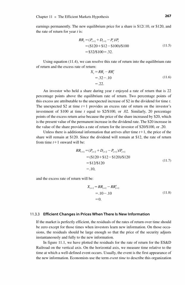
earnings permanently. The new equilibrium price for a share is $12/.10, or $120, andthe rate of return for year t is:

(11.5)

Using equation (11.4), we can resolve this rate of return into the equilibrium rateof return and the excess rate of return:

(11.6)

An investor who held a share during year t enjoyed a rate of return that is 22percentage points above the equilibrium rate of return. Two percentage points ofthis excess are attributable to the unexpected increase of $2 in the dividend for time t.The unexpected $2 at time t�1 provides an excess rate of return on the investor’sinvestment of $100 at time t equal to $2/$100, or .02. Similarly, 20 percentagepoints of the excess return arise because the price of the share increased by $20, whichis the present value of the permanent increase in the dividend rate. The $20 increase inthe value of the share provides a rate of return for the investor of $20/$100, or .20.

Unless there is additional information that arrives after time t�1, the price of theshare will remain at $120. Since the dividend will remain at $12, the rate of returnfrom time t�1 onward will be:

(11.7)

and the excess rate of return will be:

(11.8)

11.3.3 Efficient Changes in Prices When There Is New Information

If the market is perfectly efficient, the residuals of the rates of return over time shouldbe zero except for those times when investors learn new information. On those occa-sions, the residuals should be large enough so that the price of the security adjustsinstantaneously and fully to the new information.

In figure 11.1, we have plotted the residuals for the rate of return for the ES&DRailroad on the vertical axis. On the horizontal axis, we measure time relative to thetime at which a well-defined event occurs. Usually, the event is the first appearance ofthe new information. Economists use the term event time to describe this organization

X RR RRt t te

� � ��

� �

�

1 1 1

.10 .10

0.

RR P D P Pt t t t t� � � � ��

� � �

�

�

1 ( )/

($120 $12 $120)/$120

$12/$120

2 2 1 1

..10,

X RR RRt t te� �

� �

�

.32 .10

.22.

RR P D P Pt t t t t� � �

� � �

� �

� �( )/

($120 $12 $100)/$100

$32/$100 .32.

1 1


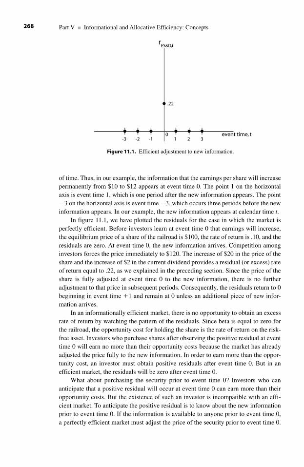
of time. Thus, in our example, the information that the earnings per share will increasepermanently from $10 to $12 appears at event time 0. The point 1 on the horizontalaxis is event time 1, which is one period after the new information appears. The point�3 on the horizontal axis is event time �3, which occurs three periods before the newinformation appears. In our example, the new information appears at calendar time t.

In figure 11.1, we have plotted the residuals for the case in which the market isperfectly efficient. Before investors learn at event time 0 that earnings will increase,the equilibrium price of a share of the railroad is $100, the rate of return is .10, and theresiduals are zero. At event time 0, the new information arrives. Competition amonginvestors forces the price immediately to $120. The increase of $20 in the price of theshare and the increase of $2 in the current dividend provides a residual (or excess) rateof return equal to .22, as we explained in the preceding section. Since the price of theshare is fully adjusted at event time 0 to the new information, there is no furtheradjustment to that price in subsequent periods. Consequently, the residuals return to 0beginning in event time �1 and remain at 0 unless an additional piece of new infor-mation arrives.

In an informationally efficient market, there is no opportunity to obtain an excessrate of return by watching the pattern of the residuals. Since beta is equal to zero forthe railroad, the opportunity cost for holding the share is the rate of return on the risk-free asset. Investors who purchase shares after observing the positive residual at eventtime 0 will earn no more than their opportunity costs because the market has alreadyadjusted the price fully to the new information. In order to earn more than the oppor-tunity cost, an investor must obtain positive residuals after event time 0. But in anefficient market, the residuals will be zero after event time 0.

What about purchasing the security prior to event time 0? Investors who cananticipate that a positive residual will occur at event time 0 can earn more than theiropportunity costs. But the existence of such an investor is incompatible with an effi-cient market. To anticipate the positive residual is to know about the new informationprior to event time 0. If the information is available to anyone prior to event time 0, a perfectly efficient market must adjust the price of the security prior to event time 0.


Figure 11.1. Efficient adjustment to new information.

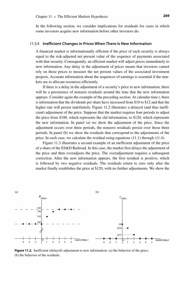
In the following section, we consider implications for residuals for cases in whichsome investors acquire new information before other investors do.

11.3.4 Inefficient Changes in Prices When There Is New Information

A financial market is informationally efficient if the price of each security is alwaysequal to the risk-adjusted net present value of the sequence of payments associatedwith that security. Consequently, an efficient market will adjust prices immediately tonew information. Any delay in the adjustment of prices means that investors cannotrely on those prices to measure the net present values of the associated investmentprojects. Accurate information about the sequences of earnings is essential if the mar-kets are to allocate resources efficiently.

If there is a delay in the adjustment of a security’s price to new information, therewill be a persistence of nonzero residuals around the time that the new informationappears. Consider again the example of the preceding section. At calendar time t, thereis information that the dividends per share have increased from $10 to $12 and that thehigher rate will persist indefinitely. Figure 11.2 illustrates a delayed (and thus ineffi-cient) adjustment of the price. Suppose that the market requires four periods to adjustthe price from $100, which represents the old information, to $120, which representsthe new information. In panel (a) we show the adjustment of the price. Since theadjustment occurs over three periods, the nonzero residuals persist over those threeperiods. In panel (b) we show the residuals that correspond to the adjustments of theprice. In each case, we calculate the residual using equations (11.1) through (11.4).

Figure 11.3 illustrates a second example of an inefficient adjustment of the priceof a share of the ES&D Railroad. In this case, the market first delays the adjustment ofthe price and then overadjusts the price. The overadjustment requires a subsequentcorrection. After the new information appears, the first residual is positive, whichis followed by two negative residuals. The residuals return to zero only after themarket finally establishes the price at $120, with no further adjustments. We show the


Figure 11.2. Inefficient (delayed) adjustment to new information: (a) the behavior of the price; (b) the behavior of the residuals.

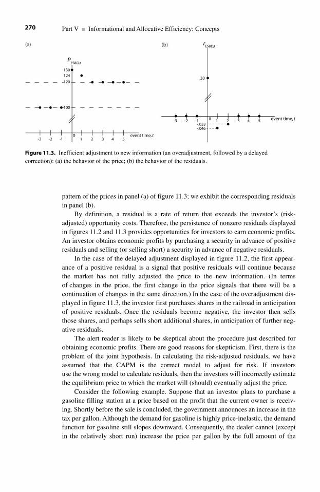
pattern of the prices in panel (a) of figure 11.3; we exhibit the corresponding residualsin panel (b).

By definition, a residual is a rate of return that exceeds the investor’s (risk-adjusted) opportunity costs. Therefore, the persistence of nonzero residuals displayedin figures 11.2 and 11.3 provides opportunities for investors to earn economic profits.An investor obtains economic profits by purchasing a security in advance of positiveresiduals and selling (or selling short) a security in advance of negative residuals.

In the case of the delayed adjustment displayed in figure 11.2, the first appear-ance of a positive residual is a signal that positive residuals will continue because the market has not fully adjusted the price to the new information. (In termsof changes in the price, the first change in the price signals that there will be acontinuation of changes in the same direction.) In the case of the overadjustment dis-played in figure 11.3, the investor first purchases shares in the railroad in anticipationof positive residuals. Once the residuals become negative, the investor then sellsthose shares, and perhaps sells short additional shares, in anticipation of further neg-ative residuals.

The alert reader is likely to be skeptical about the procedure just described forobtaining economic profits. There are good reasons for skepticism. First, there is theproblem of the joint hypothesis. In calculating the risk-adjusted residuals, we haveassumed that the CAPM is the correct model to adjust for risk. If investors use the wrong model to calculate residuals, then the investors will incorrectly estimatethe equilibrium price to which the market will (should) eventually adjust the price.

Consider the following example. Suppose that an investor plans to purchase agasoline filling station at a price based on the profit that the current owner is receiv-ing. Shortly before the sale is concluded, the government announces an increase in thetax per gallon. Although the demand for gasoline is highly price-inelastic, the demandfunction for gasoline still slopes downward. Consequently, the dealer cannot (exceptin the relatively short run) increase the price per gallon by the full amount of the


Figure 11.3. Inefficient adjustment to new information (an overadjustment, followed by a delayed correction): (a) the behavior of the price; (b) the behavior of the residuals.

increase in the tax without suffering a reduction in the volume of gasoline sold perweek. Some of the costs of operating a gasoline station are fixed (such as propertytaxes, the opportunity cost of the capital invested in the land, etc.). The greater thefixed costs, the more important the volume of sales in the generation of a profit. If theinvestor assumes that the full amount of the tax can be passed on to the consumer withno loss in sales, she is using the wrong model. Using the wrong model will lead her topay too high a price for the station. Her revenue could fall short of her opportunitycosts, making her profit negative.

The second problem in using residuals as the basis of an investment strategy isthat calculating residuals is costly. Explicit costs are incurred to collect the data andperform the calculations, and opportunity costs are incurred to analyze those data.

Third, the strategies implied by figures 11.2 and 11.3 require frequent purchasesand sales. Each of these transactions incurs costs in the form of brokers’ commissionsand taxes.

Finally, an investor who trades in anticipation of nonzero residuals must hold aportfolio that is inefficient in the context of modern portfolio theory. According to the CAPM, the investor should hold risky securities in the proportions determined by the market portfolio. An investor who temporarily purchases or sells securities in pursuit of nonzero residuals necessarily holds a portfolio that does not offer anefficient combination of expected rate of return and risk. Consequently, an investorwho pursues excess profits by trading on residuals incurs a cost in the form of accept-ing a lower expected rate of return on the portfolio given the level of risk in that portfolio.

11.4 A Second Example of Informational Efficiency: Predictability of Returns—Bubbles or Rational Variations of Expected Returns?

The early empirical tests of the efficient markets hypothesis supported the propositionthat risk-adjusted rates of return are not predictable (aside from a small upward driftimparted by the historical tendency of the economy to grow over long periods oftime). In the CAPM, each security’s beta has a constant value over time. After allow-ing for changes in the rate of return on the market portfolio from one period to thenext, any variation in the rate of return on a security is attributable solely to firm-specific risk, which is unpredictable. The efficient markets hypothesis stimulated alarge amount of empirical work, which demonstrated that to some extent rates ofreturn are predictable, even after adjusting for risk. Consequently, the major currentissue in the debate about the efficient markets hypothesis is whether the predictabilityof rates of return is evidence of (irrational) bubbles or a consequence of rational vari-ations in expected returns. That is, are we predicting (risk-adjusted) rates of returneven though each security’s beta is constant over time, or are we in fact predictingshifts in the values of beta for those securities? In this section, we discuss this questionin the context of a simple example based on the relationship between the size of a firmand its expected rate of return.


11.4.1 The Size Effect as an Example of a Rational Change in Expected Returns

Early empirical tests of the CAPM were encouraging. The average rate of return on asecurity appeared to be linearly related to the value of the beta for that security.Equivalently, the difference in the average rates of return for any two securities wasproportional to the difference in the beta values for those securities, just as the securitymarket line of the CAPM predicts. Of course, no one would expect a linear model assimple as the CAPM to predict exactly the empirical relationship between the levels ofrisk and the average rates of return across all securities. Thus, economists were notsurprised to find some dispersion of the data points for beta and average rate of returnaround the security market line.

Subsequent and closer examination of the empirical tests of the CAPM revealedthat the dispersion of the data points around the security market line was not random.There is a systematic relationship between the size of a firm and the location of thedata point for that firm relative to the security market line. The size of a firm is theaggregate market value of its outstanding securities. (In the simplest applications, the size of a firm is the price of its common stock multiplied by the number of sharesoutstanding.) The data points for small firms were more likely to be above the securitymarket line than below it.

The height of the security market line over a given value of beta is the equilibriumvalue of the average rate of return that an investor should receive in exchange for bear-ing the level of risk represented by that value of beta. Consequently, a security is under-priced if the point representing its beta and its average rate of return is located abovethe security market line. (The average rate of return on that security is too high relativeto the level of risk in that security.) According to the CAPM, the market systematicallyunderprices the securities of small firms. Economists call this phenomenon the sizeeffect.

The size effect has two competing implications that correspond to the two parts ofthe joint hypothesis. The first implication is that the market is systematically ineffi-cient because the securities of small firms are underpriced. The second implication isthat the CAPM is an incorrect specification of the relationship between risk and aver-age return.

An essential property of equilibrium in any market is that no one has an incentiveto change the allocation of her resources. Applied to a financial market, equilibriumrequires that the relative prices of securities are such that no investor can obtain anexcess risk-adjusted return by holding the securities of small firms in proportionslarger than those which appear in the market portfolio. But this condition is violated ifthe market systematically misprices the securities of small firms. If the combinationsof beta and average return for small firms lie above the security market line, then thecombination of risk and average return for a portfolio of small firms will lie above thecapital market line. A portfolio that lies above the capital market line offers an excessrisk-adjusted average return, in violation of the definition of equilibrium.

Just as nature abhors a vacuum, economists abhor the notion that a market can besystematically out of equilibrium. One way to resolve an apparent disequilibrium is toreexamine the model used to define the equilibrium.


As we saw in chapter 10, Eugene Fama and Kenneth French proposed and tested multifactor asset-pricing models that include a factor for the size of the firm.These models have resolved several of the anomalies in the empirical testing of theCAPM.

11.4.2 A Change in the Size of a Firm as an Example of a Rational Change in the Expected Return

In this section, we present a simple example of how what might appear to be a pre-dictable nonzero residual for a security could, in fact, be a rational variation in therisk-adjusted expected rate of return for that security. Suppose that investors regardsmall firms as riskier than large firms. Specifically, the expected rate of return thatinvestors require to hold the security of a given firm depends both on the beta for thatfirm and on the size of the firm. If two firms have the same value for beta, investorswill require a higher expected rate of return to hold the security of the smaller firm.Consider the following simple adjustment to the expected rate of return based on thesize of the firm.

Let Pi be the price per share of the stock of Firm i, and let Ni be the number ofshares outstanding. Then the size of Firm i is:

Si �Pi Ni. (11.9)

Let Save be the average size of the firms in the economy. Let � be a positive con-stant. Suppose that the equilibrium expected rate of return for Firm i is:

Ei�Rf�(EM�Rf )�i��(Save�Si ), (11.10)

The first two terms on the right side of equation (11.10) are the equation for thesecurity market line of the CAPM. The third term on the right side of (11.10) is theadjustment to the expected rate of return based on the size of Firm i relative to theaverage size of firms in the economy. Since � is positive, the term �(Save�Si) adjuststhe equilibrium expected rate of return upward for firms that are smaller than the aver-age size of firms, and downward for firms that are larger than the average.

We emphasize that the model specified by equation (11.10) is only an example ofhow one might construct an alternative to the CAPM in an attempt to eliminate therisk-adjusted residuals that are systematically related to the size of firms in that model.In chapter 10 we discussed the three-factor model proposed by Fama and French thatadjusts the equilibrium returns defined by the CAPM by adding terms for the size ofthe firm and for the ratio of the firm’s book equity to its market equity.

Predictable risk-adjusted residuals are incompatible with an informationally effi-cient market. We will now use the model in equation (11.10) to present an example ofhow the existence of predictable residuals could be reconciled with an efficient market.

The model in equation (11.10) states that the expected rate of return for Firm iwill change if the size of that firm changes (relative to the average size of firms).Suppose there is evidence that some variable, call it Z, is correlated with subsequentvalues of residuals under the CAPM. Specifically, let Zi,t be the value of Z for Firm iat time t. Let Xi,t be the risk-adjusted residuals for Firm i at time t according to theCAPM. Finally, suppose that for some ��0, the variable Zi,t is highly correlated with


the values of Xi,t�1, . . . , Xi,t�τ. Then an investor could use information about Zi,t topredict the residuals for Firm i during the interval from time t�1 through time t�τ.This ability to predict residuals violates the efficient markets hypothesis under theCAPM. But suppose that the modified CAPM in equation (11.10) is the correct modelof equilibrium. Then the apparent ability to predict residuals by using the variable Z isspecious. Let Zi,t be correlated with future changes in the size of Firm i. If equation(11.10) is the correct model of equilibrium, then information about Zi,t is informationabout the future expected rate of return for Firm i. An informationally efficient market is rational in the sense that the prices of securities reflect the availableinformation about the values of the correctly risk-adjusted net present values of theassociated sequences of payments. Nonzero residuals can be a rational response tonew information.

11.5 Informational Efficiency and the Predictability of Returns

In this section, we provide a brief review of the main issues in the literature on theefficient markets hypothesis. For a rigorous and comprehensive treatment of this liter-ature, readers should work through the paper by Eugene Fama, cited earlier, and theliterature that has appeared subsequent to that paper.

11.5.1 A Brief Synopsis of the Debate

Following Fama, the debate about the efficient markets hypothesis is between thosewho argue that the predictability of returns (or equivalently, the predictability of resid-uals) is evidence of rational adjustment of expected rates of return to new information,and those who argue that the predictability of returns indicates bubbles. The debatehas two dimensions. One dimension is the predictability of returns for given securitiesover time. The other is the predictability of returns across securities at a given time.The economists on each side of the debate have sophisticated empirical studies to sup-port their positions. Nevertheless, as we explained earlier in this chapter, all tests ofinformational efficiency involve the joint hypothesis, and consequently many ques-tions cannot be finally resolved.

11.5.2 The Challenge from Thaler and deBondt

The economists Richard Thaler and Werner deBondt raised a challenge to the EfficientMarkets Hypothesis by presenting evidence of irrational behavior by investors.12

Specifically, investors systematically form incorrect expectations about the continuationof recent movements in security prices. This research has led to a new set of hypothesescalled behavioral finance, in which psychological considerations compete with theoret-ical asset pricing models to explain the empirical behavior of rates of return.13

Thaler and deBondt show that stocks that have abnormally high rates of returnover a period of years have abnormally low rates of return over a subsequent period ofyears, and that the converse is also true.14 These economists suggest that investors


irrationally project recent movements too far into the future. Consequently, investorspurchase stocks that have recorded high returns in the expectation that the highreturns will persist. These (irrational) purchases of recent winners in pursuit of a con-tinuation of the high returns forces the prices of these stocks far above their equilib-rium values. The ensuing correction brings prices back down, causing abnormallylow, or even negative, returns until the market reestablishes the prices at their equi-librium values.

Similarly, investor sell (or sell short) stocks whose recent returns are abnormallylow, forcing the prices of these stocks far below their equilibrium values. The subse-quent correction creates abnormally high returns until the prices regain their equilib-rium values.

Of course, an “abnormal” rate of return is a return that differs from the risk-adjusted rate of return predicted by an asset pricing model. But which model is thecorrect one? Other economists claim that the phenomenon reported by Thaler anddeBondt is attributable to a failure to adjust the returns correctly for risk, particularlyfor the sizes of the firms. Thaler and deBondt disagree, and the question is clouded bythe joint hypothesis.

11.5.3 The Challenge from Summers and Shiller

There is evidence that residuals are autocorrelated. That is, information about currentor past residuals is of some value in predicting the future values of those residuals. Aninvestor can use these autocorrelations to obtain excess returns if the transaction costsare low enough. Some economists argue that, although the correlations are reliable,they are too close to zero to overcome the transaction costs, and thus the statisticalrelationship among the residuals has no economic significance.15

Summers and Shiller reject the argument that the market can be informationallyefficient even in the presence of reliable, but small, autocorrelations.16 These econo-mists “present simple models in which prices can take large slowly decaying swingsaway from fundamental values (fads or irrational bubbles) but short-horizon returnshave little autocorrelation.”17 If prices do take large departures from fundamental val-ues, and return only slowly to those values, then the market is informationally ineffi-cient, because investors cannot rely on security prices to provide accurate informationabout the net present values of sequences of payments.

11.5.4 Conclusion Thus Far

In this subsection, we have presented a brief context for the debate on the implicationsof the predictability of returns for the efficient markets hypothesis. The literature inthis area is so voluminous and specialized that a comprehensive survey is far beyondthe scope of this book.

Three conclusions are probably safe, however. First, however the debate proceedsfrom its current state, the CAPM has generated both theoretical and empirical researchthat has significantly advanced our knowledge of how financial markets set the pricesof securities. In particular, both academics and professionals have accepted the


principle that the correct measure of risk of a security involves a correlation betweenthe rate of return on that security and the rates of return on one or more special port-folios.

The second conclusion is that after taking transaction costs into account, the market is efficient enough to eliminate all opportunities for excess returns except forinvestors who either have very low transaction costs or who have a strong comparativeadvantage in acquiring and analyzing new information rapidly and accurately.

The third conclusion addresses the value created by speculators. Readers shouldrecall from their introductory courses that the basis of a mutually beneficial exchangeof a good is that two (or more) persons differ either in the marginal costs at which theycan produce that good, or in the marginal values that they place on that good, or both.The good in question can be an informationally efficient financial market. Allinvestors benefit from an efficient market. Some investors specialize in discoveringprices that do not fully reflect the information about the net present values of the asso-ciated sequences of payments. Economists define as speculators the investors whosearch for these incorrect prices. Competition among speculators forces prices toreflect the information that the speculators have acquired. Thus speculators produce agood by making markets more efficient than they would otherwise be.

What about the investors whose comparative advantage in speculating is soweak that they trade in the wrong direction, creating pressure on prices to depart further from net present values? These adverse movements of prices create evenmore opportunities for the more competent speculators to gain profits. The actions ofthe competent speculators will imposes losses on the incompetent ones, thus weedingthem out.

11.6 Informational Efficiency and the Speed of Adjustment of Prices to Public Information

Public information is information that is available to the typical investor at little or nocost to that investor. Examples of public information include announcements by firmsof projected or realized earnings, changes in financial structure, changes in senior man-agement, and the status of litigation. Announcements by governmental agencies suchas the Federal Reserve and the Departments of Commerce and Labor are also publicinformation. In short, public information includes everything that the typical investorcan obtain for the price of a newspaper or the cost of turning on a television set.

The efficient markets hypothesis requires that “prices reflect information to thepoint where the marginal benefits of acting on information (the profits to be made) donot exceed the marginal costs.”18 The empirical tests of the efficient markets hypoth-esis with respect to public information involve event studies, which we present in thenext chapter. The consensus among economists is that the efficient markets hypothe-sis is verified with respect to public information. Consequently, unless an investor hasan unusually strong comparative advantage in obtaining public information quickly,analyzing correctly its likely effect on prices, and trading quickly on that informationat low transaction costs, it is highly unlikely that the investor will obtain profits thatcover the marginal costs.


11.7 Informational Efficiency and the Speed of Adjustment of Prices to Private Information

The most demanding form of the efficient markets hypothesis is that the prices ofsecurities fully reflect all information, including private information.19 Under thisform of the hypothesis, even persons with access to private information, such as officers of corporations and principals of investment banks, could not obtain (risk-adjusted) excess returns. Unsurprisingly, the empirical evidence does not support theefficient markets hypothesis with respect to private information. In this section, weprovide a brief review of the evidence.

11.7.1 Insider Trading

There is strong evidence that corporate insiders do trade on private information, andthat they do so profitably.20 To trade profitably requires purchasing (or selling) a security in advance of the market’s adjusting the price of that security to positive (ornegative) information. That is, the insiders are able to predict nonzero risk-adjustedresiduals. Since predictable residuals violate the efficient markets hypothesis, themarket is not efficient with respect to private information.

That the market does not fully reflect private information did not surprise econo-mists. What did surprise economists was evidence presented by Jeffrey Jaffe thatinvestors who are not corporate insiders could also obtain nonzero residuals by mim-icking the trades of the insiders for up to eight months after the insiders’ tradesbecame public knowledge.21 This is a violation of the less demanding form of the effi-cient markets hypothesis, namely that security prices fully (and immediately) reflectall public information.

The Securities and Exchange Act of 1934 defines insiders as the senior officersand the directors of corporations, and persons who hold more than 10% of the stock.The act requires insiders to report their trades to the Securities and ExchangeCommission by the tenth day of the month following the month in which the tradeoccurred. (Most insiders report their trades within a few days of the trades.) Thecommission publishes these reports one day after receiving them. Any investor canuse these public reports to mimic the insiders’ trades. If the market is efficient withrespect to public information, the prices of the securities in which the insiders tradedshould fully reflect the information on which the insiders traded. Consequently, itshould be impossible for outsiders to obtain nonzero residuals by mimicking theinsiders’ trades.

Economists treated as anomalous the market’s apparent failure to adjust securityprices to reflect the insiders’ information soon enough to prevent opportunities foroutsiders to mimic insiders profitably. As is usual with anomalies, economists dili-gently searched for explanations. The resolution is an example of the confoundingeffect of the joint hypothesis. Specifically, the anomaly arises because the distributionof insiders’ purchases and sales is systematically related to the sizes of firms, and theCAPM has no adjustment for the size of the firm.

Purchases of securities by insiders are more likely to occur in small firms, whilesales by insiders are more likely to occur in large firms. Jaffe used the CAPM to


measure residuals. Recall that the CAPM systematically underprices small firms.Using these facts, N. Nejat Seyhun demonstrated that the ability of outsiders to obtainrisk-adjusted residuals by mimicking insiders depends on using the CAPM to measurethe residuals.22 That is, the anomaly is not robust with respect to the choice of modelto define equilibrium.

11.7.2 Security Analysts

The question here is, can security analysts identify mispriced securities with sufficientprecision to allow their clients to obtain excess (risk-adjusted) returns net of transac-tion and opportunity costs? There is strong evidence that the answer is no, althoughthere are a few anomalies. The apparent ability of the Value Line Investment Survey toidentify mispriced securities is best known of these anomalies. The anomaly has beenthe subject of many empirical tests. Some economists argue that the residuals thatinvestors can predict by using Value Line are not, in fact, excess returns. Rather, theseresiduals are indications of rational changes in risk-adjusted expected returns.

There is no clear resolution to the Value Line anomaly. Significantly, one econo-mist “reports that the strong long-term performance of Value Line’s group 1 stocks isweak after 1993. Over the 6.5 years from 1984 to mid-1990, group 1 stocks earned16.9% per year compared with 15.2% for the Wilshire 5000 index. During the sameperiod, Value Line’s Centurion Fund, which specializes in group 1 stocks, earned12.7% per year—live testimony to the fact that there can be large gaps between simu-lated profits from private information and what is available in practice.”23

The preponderance of the evidence is that investors cannot obtain excess returnsby relying on analysts. Quoting again from Fama:

The evidence is that Value Line and some security analysts have privateinformation that, when revealed, results in small but statistically reliableprice adjustments. These results are consistent with the “noisy rationalexpectations” model of competitive equilibrium of Grossman and Stiglitz(1980). In brief, because generating information has costs, informedinvestors are compensated for the costs they incur to ensure that pricesadjust to information. The market is then less than fully efficient (there canbe private information not fully reflected in prices), but in a way that is consistent with rational behavior by all investors.24

The term rational behavior includes the condition that it is only excess returns netof opportunity costs (including transaction costs) that should count as evidenceagainst the efficient markets hypothesis.

We conclude this section with some disturbing evidence against the hypothesisthat investors are rational. Economists Brad M. Barber and Terrance Odean examinedthe performance of a large sample of investors who managed their own portfoliosrather than investing indirectly through mutual funds and pension funds. According tothese economists, in 1996 almost one-half of the common stocks in the United Stateswere owned directly by households. The evidence is that the majority of these house-holds traded so frequently that they did significantly less well than they would havedone if they held more passive portfolios, such as they could have done by investing


in mutual funds that track the major indexes. Barber and Odean titled the article“Trading Is Hazardous to Your Wealth.” Quoting from the abstract:

Individual investors who hold common stocks directly pay a tremendousperformance penalty for active trading. Of 66,465 households with accountsat a large discount broker during 1991 to 1996, those that trade most earn anannual return of 11.4%, while the market returns 17.9%. The average household earns an annual return of 16.4%, tilts its common stock investment toward high-beta, small, value stocks, and turns over 75% of itsportfolio annually. Overconfidence can explain high trading levels and theresulting poor performance of individual investors. Our central message istrading is hazardous to your wealth.25

11.7.3 Professional Portfolio Management

Finally, we briefly review the tests of the efficient markets hypothesis regardingmutual funds and pension funds. The question is whether the professional managers ofthese funds possess private information that enables them to outperform the market.Since we measure performance on a risk-adjusted basis, the empirical work on thisquestion necessarily encounters the problems of the joint hypothesis.

Michael Jensen performed the seminal work on this question in 1968 and 1969.26

In his study of mutual funds, and using the CAPM to define risk-adjusted rates ofreturn, Jensen found that the average returns to investors in mutual funds, after sub-tracting the management fees and other expenses that the funds assess on theirinvestors, fall about 1% below the security market line.27 “Jensen concludes thatmutual fund managers do not have private information.”28

Studies subsequent to that of Jensen have presented evidence that mutual fundmanagers can generate returns gross of expenses that lie above the security marketline, and therefore do have private information that the market has not reflected insecurity prices. At the level of the individual investor, however, it is returns net ofexpenses that matter. The evidence supports the conclusion that the expenses, whichinclude the compensation of the managers, absorb the value of the managers’ privateinformation, leaving the net returns close to the security market line. There is alsosome evidence that any excess returns obtained by mutual funds are negatively relatedto expenses and turnover. This result suggests that the managers of these funds investtoo much of the investors’ funds in the search for mispriced securities.

11.8 Information Trading, Liquidity Trading, and the Cost of Capital for a Firm

In this subsection, we explain the relationship among the informational efficiency of afinancial market, the liquidity of a firm’s securities, and the firm’s cost of capital. Thefirst step is to explain the concept of the cost of capital for a firm.


11.8.1 The Cost of Capital for a Firm

The cost of capital for a firm is the rate of return that the firm must offer to investorsto induce them to finance a project. The firm can infer the value of its cost of capitalfrom the ratio of its earnings per share to the market price of a share. For example,suppose that the earnings per share of the ES&D Railroad are $12, and the price of ashare of the railroad’s stock is $100. Then the investors who hold the railroad’s stockreceive a rate of return of .12 on their investment. We conclude that the rate of returnof .12 covers the investors’ opportunity costs, because otherwise competition amongthe investors to sell their shares and invest the funds elsewhere would drive the priceof the share down from $100. As the price of the share decreases, the ratio of the rail-road’s earnings per share to the price of a share increases until the rate of return forinvestors who hold those shares covers their opportunity costs.

We know that a firm can increase the wealth of its shareholders by undertakingany project that has a positive net present value. If the railroad issues new securities tofinance a project, those securities become additional claims on the earnings of theentire firm. That is, both the new securities and the previously issued securities areclaims to the earnings of the railroad’s portfolio of projects. Usually, the firm cannot(or does not) issue securities that are claims to the earnings of a specific project.29

Consequently, when calculating the net present value of a proposed project, it iscritical that the firm use the cost of capital implied by the price of the firm’s shares todiscount the future earnings expected from the project. If a firm uses a discount ratethat is less than its cost of capital when calculating the present value of a project, thefirm will overstate the effect on its shareholders’ wealth of undertaking that project. Ifthe overstatement is sufficiently large, undertaking that project will cause the share-holders to lose wealth.30

Consider the following example. Prior to the unexpected imposition of a tax onthe earnings of railroads, the ES&D Railroad planned to improve its roadbed to permitan increase in the speeds at which trains can operate. The railroad planned to financethe project by selling new securities. As we explained above, the price of the railroad’sshares implied that the railroad’s cost of capital is .12. Using that rate of return, theproposed project had a positive net present value. Therefore, had the tax not beenimposed, the railroad could have increased its shareholders’ wealth by undertaking theproject.

The imposition of the tax reduces the railroad’s earnings per share from $12 to$10, and as a result the price of a share falls from $100 to $83.33. At the lower priceper share, the shareholders are again receiving a (net of tax) rate of return of .12. Hadthere been no change in the price of the railroad’s outstanding securities to reflect theeffect of the tax, the investors who hold the railroad’s securities would have suffered areduction in the rate of return on their investment. These investors would then havehad an incentive to sell their shares in the ES&D Railroad and invest their funds in thesecurities of other firms whose earnings are not subject to the tax. But no investorswould purchase the railroad’s securities unless their price fell by enough to offset theeffect of the tax. Consequently, the announcement of the tax will reduce the price of arailroad’s outstanding securities. Moreover, if the market is informationally efficient,the price of the share will change immediately from $100 to $83.33.31


Since the additional earnings created by the project will be subject to the new tax,the net present value of the project will be less than it would have been without thetax. If the net present value of the project inclusive of the tax is negative, the railroadcan no longer undertake the project profitably.

In effect, the imposition of the tax increases the firm’s cost of capital. Without thetax, the net present value of the project is positive when the future earnings of theproject are discounted at a rate of .12. That is, the project generates a rate of return thatis greater than .12. If the railroad’s cost of capital were, say, .15, the project wouldhave to generate earnings at a rate greater than .15 if its net present value is to be pos-itive. Since the net present value varies inversely with the rate at which the future pay-ments are discounted, increasing the discount rate sufficiently would cause the netpresent value of the project to become negative. If the tax is high enough to make thenet present value negative, the effect of the tax is the same as an increase the firm’scost of capital. Namely, the project must generate earnings at a higher rate if its netpresent value is to be positive. In the following section, we explain how a decrease inthe liquidity of the firm’s securities increases the firm’s cost of capital, just as a tax onthe firm’s earnings has the effect of increasing the cost of capital.

As a second example, suppose that investors believe that the railroad’s earningswill become more sensitive to unpredictable fluctuations in the performance ofthe macroeconomy. Under the CAPM, the railroad’s beta will increase, which willrequire an increase in the expected rate of return on the railroad’s securities. In theabsence of an increase in the expected earnings of the railroad, the price of its securi-ties must fall if the expected rate of return is to increase. Suppose that the price of ashare falls from $100 to $80. Then the rate of return increases from $10/$100, or .10,to $10/80, or .125, and consequently the railroad’s cost of capital increases to .125.Before investors revised their beliefs about the value of the railroad’s beta, the firmcould have profitably undertaken a project whose rate of return is equal to .11.Subsequent to the revision in investors’ beliefs, that project is no longer profitable.

11.8.2 Liquidity and the Bid-Asked Spread

Liquidity is a measure of the effect on the price of an asset of an increase in the speedor the size of a transaction in that asset. A small number of shares of IBM stock is ahighly liquid asset. An attempt to purchase or sell 5,000 shares immediately, withoutnotice to prospective investors on the other side of the transaction, would have nomeasurable effect on the price at which the transaction is executed. But an offer topurchase or sell 50,000,000 shares immediately would have an effect on the price.Unlike the stock of IBM, the stocks of small firms are traded infrequently. For thesefirms, an attempt to purchase or sell 5,000 shares immediately would likely affect theprice at which the transaction is executed.

It is common to hear the remark that a house is an illiquid asset because one can-not sell it quickly. “It takes time to sell a house.” That statement is not true. The authorcould likely sell his house in a morning by accepting a sufficiently low price.Similarly, there are likely many houses that one could purchase in an afternoon bycredibly offering to pay a sufficiently high price. Houses are not difficult to sell (or to purchase) quickly. But the effect on the price of allowing time to search for


prospective buyers, and to allow those buyers to collect information about the house,is significant. That is the reason why most persons choose not to sell their homesquickly. A house is an illiquid asset because the cost of insisting on a speedy transac-tion, or of attempting to purchase or sell a large quantity, is significant.

Any asset, including a financial security, can be characterized in terms of itsliquidity. In many contexts it is sufficient to speak of the price of a security. In fact,however, each security has two prices: a bid price (or bid) at which dealers willpurchase shares for addition to their inventories, and a higher asked price (or asked) atwhich they will sell shares out of their inventories. Speaking generally, the economicfunction of a dealer in any good is to maintain a bid price at which the dealer standsready to purchase the good without prior notice, and an asked price at which he or shewill sell the good without notice. Harold Demsetz has stated that the essential functionof a dealer is to provide predictable immediacy.32

A dealer is the owner of a particular kind of firm. Accordingly, economistsanalyze dealers by assuming that they will choose the values of their bid and askedprices to maximize profit.33 To maximize profit is to maximize the difference betweenrevenues and costs. The dealer’s revenues include the markup between the bid priceand the asked price. On a given day, a dealer might purchase several shares from someinvestors by paying his bid price, and subsequently resell those same shares to otherinvestors at his asked price. The dealer will set his bid and asked prices so that thequantities of shares that he purchases over several hours during a typical day, or overa few days in a typical week, will be equal to the quantities of shares that he sells. Ifthe dealer does not adjust his bid and asked prices to equate the quantities supplied tohim with the quantities demanded from him, the level of his inventory will eitherincrease or decrease to levels that he is not willing to tolerate.34

Capital gains are another source of revenue for the dealer. Dealers will obtain acapital gain if they can purchase shares in advance of the publication of positive infor-mation about the net present value of the sequence of payments associated with thoseshares. If dealers can obtain this information before the typical investor does, they canpurchase the shares at a bid price that does not reflect the information, and later resellthose shares at an asked price that does reflect the information. Once the positiveinformation becomes public knowledge, dealers can increase both the bid and theasked prices. In fact, once the information becomes public, dealers must increase theirprices to avoid a depletion of inventory to unacceptable levels.35 A dealer can alsoobtain a capital gain if he can sell the security in advance of negative information.

Just as capital gains are a source of revenue for the dealer, capital losses are asource of costs. The dealer will incur a capital loss if he fails to adjust his bid and askedprices before the publication of new information that will affect the quantities of thesecurity that investors want to hold in their portfolios. For example, suppose that thevolume of sell orders exceeds the volume of buy orders between 10:00 and 10:15 A.M.on a given day. If this excess supply of shares to the dealer is caused by a random fluc-tuation in the difference between the volumes of buy and sell orders, the fluctuation inthe size of the dealer’s inventory will be temporary, and he will soon gain revenue byreselling at his asked price the excess of shares that the purchases at his bid price.36

But suppose that the excess of sell orders over buy orders is based on negativeinformation that the dealer does not yet have. In this case, the dealer will have


purchased shares that he cannot subsequently resell at a higher asked price once theinformation becomes public.37

We conclude that to maximize profit, the dealer in a security must choose bid andasked prices that are compatible with all the information about the net present value ofthe sequence of future payments that are associated with that security. To pursue thisquestion, we must distinguish between information trading and liquidity trading.

11.8.3 Information Trading, Liquidity Trading, and the Bid-Asked Spread

Information trading is trading by investors who believe that the current bid price orthe current asked price of a security do not correctly reflect the risk-adjusted net pres-ent value of the sequence of payments associated with that security. To the extent thattheir information is correct, competition among information traders will cause theprices of securities to reflect net present values more accurately. Thus, informationtrading increases the level of informational efficiency of the market, and thereby thelevel of economic efficiency.

Liquidity trading is trading by investors to adjust either the size or the level ofrisk in their portfolios. Persons typically increase the size of their portfolios to effectintertemporal exchanges. For example, most persons who are currently earning incomedivert a portion of that income away from current consumption and into the purchaseof financial securities. In later years, these persons will sell some (or all) of thosesecurities to augment their income during those years. A person who is saving forretirement or to pay for college educations for children or grandchildren will typicallypurchase financial securities (rather than accumulating cash under the mattress).Similarly, a person will sell financial securities to provide income during retirement,or to finance large expenditures, such as purchasing a house or sending children tocollege.

Persons may want to change the level of risk in their portfolios as their circum-stances change. As they approach retirement, or move further into retirement, theymight want to reduce their level of risk. In the context of the CAPM, such a personwould move some funds out of the market portfolio and into the risk-free asset.Similarly, a person who becomes wealthier, or whose source of income becomes moresecure, would move funds out of the risk-free asset and into the market portfolio.

At any moment, the investors who want to purchase a security at the dealers’asked price will typically include both information traders and liquidity traders.38

Similarly, there are both information traders and liquidity traders offering to sell secu-rities to the dealer at his bid price. The dealer cannot perfectly distinguish between thetwo kinds of traders. To the extent that the dealer is transacting with informationtraders, he is likely to incur a capital loss because those investors are trading on supe-rior information. That is, the information traders offer to purchase the security at thedealers’ asked price, or sell at his bid price, because they know that the dealers’ pricesdo not fully reflect the traders’ information.

Dealers will seek to protect themselves against losing to the information tradersin two ways. First, they will increase the spread between their bid and asked prices.Second, they will reduce the depth at those prices. Depth is a measure of the quantitythat dealers will offer to purchase at their bid price and sell at their asked price.


For example, a dealer might quote a bid price of $100.00 and an asked price of$100.86. But unless his inventory of shares is unacceptably low, he might purchaseonly 1,000 shares at his bid price. Should an investor offer to sell 10,000 shares, thedealer might take only 1,000 shares at $100.00 and offer substantially less for theremaining 9,000 shares. Similarly, the dealer might back away from his asked price iftraders offer to purchase a large volume of shares at that price.

If a dealer in a security widens the spread between his bid and asked prices, theliquidity of that security decreases. Think of the markup between the wholesale andthe retail prices of used automobiles. The larger the spread between these prices, thegreater the cost incurred by a consumer who purchases an automobile and plans totrade it in on a newer model sometime later. Similarly, if the dealer reduces the depththat he provides at his bid and asked prices, the liquidity of the security decreases.

11.8.4 The Effects of Information Trading and Liquidity Trading on Economic Efficiency through Their Effects on the Cost of Capital

The price that investors are willing to pay for a security is inversely related to its liq-uidity. Recently married couples planning to make a down payment on a house arelikely to hold some of their assets in liquid securities, like government bonds, ratherthan illiquid securities like the stock of a small firm, even if the long-term prospects ofthat firm are highly favorable. Parents who anticipate paying for college tuition fortheir children within the next year are also likely to be sensitive to the liquidity of asecurity.

If dealers perceive that the number of information traders is increasing relative tothe number of liquidity traders, the dealers are likely to increase the spread betweentheir bid and asked prices, or decrease the depth that they are willing to provide at thoseprices, or both. The same result will occur if the dealers believe that the informationtraders are increasing the quality of their information. In either case, the decrease in theliquidity of the security will depress the price of the security and thus increase thefirm’s cost of capital. The firm’s cost of capital increases because the lower the price ofits securities, the greater is the proportion of ownership that the current shareholdersmust cede to new investors in order to finance a new project. An increase in the cost ofcapital means that some his projects that were profitable will no longer be so.

The net effect of information traders on economic efficiency is ambiguous. To theextent that information traders increase the informational efficiency of the financialmarkets, they increase the level of economic efficiency. But to the extent that informa-tion traders increase firms’ cost of capital by decreasing the liquidity of their securi-ties, information traders decrease the level of economic efficiency. We revisit thisquestion in chapter 16, where we discuss the issue of insider trading.

11.9 Distinguishing among Equilibrium, Stability, and Volatility

Discussions about financial markets are often inhibited by a confusion among theterms equilibrium, stability, and volatility. This confusion is especially damaging to an informed discussion of the efficient markets hypothesis. In this section, we offer


a distinction among these three terms that can eliminate (or at least reduce) the confusion.

11.9.1 Equilibrium

An equilibrium is a configuration of prices and quantities at which the quantity sup-plied of each good is equal to the quantity demanded. An efficient equilibrium is onethat offers no opportunities for further mutually beneficial exchanges. If a financialmarket is in an efficient equilibrium, no investor has an incentive to reallocate fundsamong securities. In an informationally efficient market, the equilibrium price of asecurity is the risk-adjusted net present value of the sequence of payments associatedwith that security. Consequently, if there is new information about the sequence of pay-ments, or about the marginal rate at which investors are willing to substitute betweencurrent and future consumption, or between risk and expected rate of return, then theefficient equilibrium values of prices will change to reflect that new information.

The current price of a security is not necessarily its efficient equilibrium price.That is, although quantities supplied and demanded of that security might be equal,the current price need not be the risk-adjusted net present value of the associatedsequence of payments. In particular, the arrival of information that changes the equi-librium price of a security does not necessarily mean that the current price will changeto reflect the new information. The market might not be informationally efficient. Thisbrings us to the definition of stability.

11.9.2 Stability

Stability is a criterion that economists use to classify equilibria. An equilibrium is sta-ble if prices are always close to their equilibrium values. We define close to mean thatthe difference between the current price and its equilibrium value is sufficiently small,or sufficiently brief, that the typical investor cannot obtain a profit by speculating inthat security. This definition of stability requires that, upon the appearance of newinformation, the market must adjust prices to their new equilibrium values quicklyenough to eliminate opportunities for speculation for the typical investor. Of course werecognize that it is not the market that adjusts the prices. Rather, it is the competition ofspeculators trading on the new information that forces prices to their new equilibriumvalues quickly enough to eliminate opportunities for the typical investor to speculateprofitably. No one will speculate unless he or she can expect to obtain a profit. Conse-quently, the stability of an equilibrium requires the existence of speculators who have asufficiently strong comparative advantage to cover their marginal costs.

11.9.3 Volatility

Volatility is a measure of the magnitude and the rate at which the price can changeunpredictably. Here we must be careful to distinguish between an equilibrium priceand the efficient equilibrium price. There is a one-to-one correspondence between theefficient equilibrium price of a security and the information about the sequence offuture payments associated with that security. Consequently, a change in the information


will change the efficient equilibrium price. By definition, new information is unpre-dictable. If new information is also volatile, in the sense that the arrival of the infor-mation and the significance of the information are highly unpredictable, then theefficient equilibrium price of the security will be commensurately volatile. Whetherthe market is efficient is a separate question, and this question bears on the confusionamong equilibrium, stability, and volatility. Consider the following examples.

Example 1. The prices of U.S. government bonds depend critically on theannouncements of the Federal Reserve Board regarding monetary policy. The marketimmediately and correctly adjusts the prices of these bonds to announcements by theFed. Suppose that the Fed were to change its policy frequently and in ways that havelarge effects on the prices of the bonds. Suppose also that the market cannot predictthe Fed’s announcements. In this situation the market is informationally efficient,because the equilibrium prices immediately and correctly reflect the new information.The bond market is also stable, because the actual prices are always close to theirequilibrium values. But bond prices are volatile, not because the market is inefficient,but because the information to which the market responds efficiently is volatile.

Example 2. Suppose that the government imposes a large tax on short-termtrading in foreign currencies. The tax discourages speculators, with the result thatprices change slowly in response to new information. In this situation, large discrep-ancies can develop between current prices and the efficient equilibrium values ofthose prices. An unsophisticated observer might describe this market as stable, mean-ing that prices are not volatile, when in fact the market is unstable by our proposeddefinitions.

We conclude that stability and informational efficiency are closely related. A sta-ble market is one in which prices are kept close to their equilibrium values, even ifthose prices are highly volatile because the information that determines those equilib-rium prices is highly volatile.

11.10 Conclusion

In this chapter, we have discussed the importance of informational efficiency for aneconomically efficient allocation of resources. We examined some of the empiricalwork that addresses the extent to which financial markets are informationally effi-cient. The empirical work is constrained by the joint hypothesis, which requires thatevery empirical test of informational efficiency is necessarily also a test of the modelof equilibrium that the investigator uses to measure abnormal returns (risk-adjustedresiduals). There is evidence that residuals are reliably predictable, which wouldappear to violate the efficient markets hypothesis except for two considerations. First,it is unclear whether the predictability of residuals is a consequence of an inefficientmarket or evidence of rational changes in the risk-adjusted equilibrium expected ratesof return. The joint hypothesis creates difficulties that, at this stage of our understand-ing of financial markets, are insurmountable. Second, there is a distinction betweenstatistically significant and economically significant predictability. An information-ally efficient market will cause prices to reflect information up to, but not beyond, the


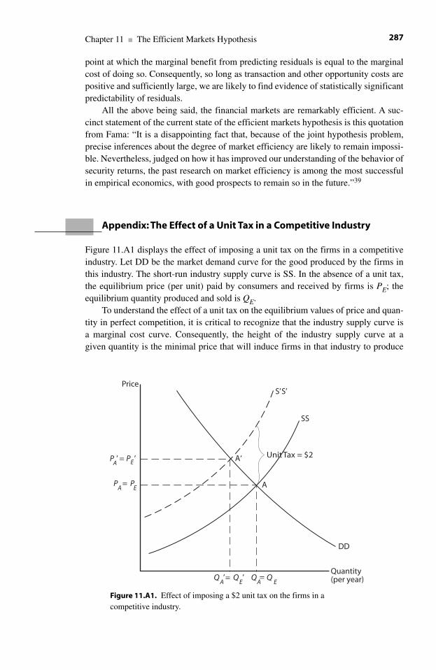
point at which the marginal benefit from predicting residuals is equal to the marginalcost of doing so. Consequently, so long as transaction and other opportunity costs arepositive and sufficiently large, we are likely to find evidence of statistically significantpredictability of residuals.

All the above being said, the financial markets are remarkably efficient. A suc-cinct statement of the current state of the efficient markets hypothesis is this quotationfrom Fama: “It is a disappointing fact that, because of the joint hypothesis problem,precise inferences about the degree of market efficiency are likely to remain impossi-ble. Nevertheless, judged on how it has improved our understanding of the behavior ofsecurity returns, the past research on market efficiency is among the most successfulin empirical economics, with good prospects to remain so in the future.”39

Appendix: The Effect of a Unit Tax in a Competitive Industry

Figure 11.A1 displays the effect of imposing a unit tax on the firms in a competitiveindustry. Let DD be the market demand curve for the good produced by the firms inthis industry. The short-run industry supply curve is SS. In the absence of a unit tax,the equilibrium price (per unit) paid by consumers and received by firms is PE; theequilibrium quantity produced and sold is QE.

To understand the effect of a unit tax on the equilibrium values of price and quan-tity in perfect competition, it is critical to recognize that the industry supply curve is a marginal cost curve. Consequently, the height of the industry supply curve at a given quantity is the minimal price that will induce firms in that industry to produce


PA’ = PE ’

PA

= PE

QA’ ’ = Q

E A = QQ

E

A

A‘

DD

Unit Tax = $2

SS

S’S’

Quantity(per year)

Price

Figure 11.A1. Effect of imposing a $2 unit tax on the firms in a competitive industry.

that quantity.40 To understand this interpretation, consider the following brief reviewof profit maximization by firms in a perfectly competitive industry.

In a perfectly competitive market, every firm behaves as if it could sell an unlim-ited quantity of its output at the market price. To maximize its profit, each firm willproduce and sell the quantity of its output at which the marginal cost incurred by thatfirm is equal to the market price. Consequently, the marginal cost at a given quantity,say q1, is the minimal price per unit that will induce that firm to produce q1 units (perunit of time). By definition, the marginal cost at the quantity q1 is the additional costthat the firm would incur to produce q1 units of output (per unit of time) rather than q1�1 units (per unit of time). If the firm’s marginal cost curve is upward sloping,producing a quantity for which marginal cost is equal to the price assures the firm of aprofit on each unit produced except the final (or the marginal) unit.41 The profitgained from q1 units (per unit of time) rather than q1�1 units is zero. Were the firm toincrease the rate of output beyond q1, the profit on that final unit would be negative,and thus the firm’s total profit would not be as large as it would be had the firm pro-duced at the rate q1.42

A consequence of the preceding analysis of the individual firm is that the heightof the industry supply curve at any given quantity is the minimal price that the indus-try will require to produce that rate of output. Consider Point A on the supply curve,SS. If the price is PA, each firm will produce a rate of output for which that firm incursa marginal cost equal to PA. Therefore, if each firm’s marginal cost curve slopesupward, no firm will increase its rate of output unless the market price increases. Forany firm to do so would cause a decrease in that firm’s total profit. Therefore, PA is theminimal price required by the industry to produce QA units.

The sum of the quantities supplied by all firms in the industry, when the price isPA, will be QA. The marginal cost for the industry is the increase in total cost that allfirms in the industry together would incur if the rate of output of the industry were toincrease by one unit. The industry can increase its rate of output by one unit simply byhaving any one firm increase its output by one unit (with the other firms making nochanges in their rates of output). When the market price is PA, the marginal cost forevery firm in the industry is PA. Therefore, when the market price is PA, the marginalcost for the industry is also equal to PA.43

Now suppose that the government imposes on each firm a unit tax equal to $2.The imposition of this tax requires each firm to pay to the government $2 for each unitsold. Whether a firm passes all of this tax, some of it, or none of it to consumers in theform of a higher price is a matter of indifference to the government. The governmentonly requires that each firm pay to the government $2 for each unit that that firm pro-duces. In effect, the $2 tax is a fee that the government charges each firm for the rightto produce a unit of the product.

Consider again Point A on the supply curve SS. We established that the price PAis the minimal price that will induce firms in the industry to produce the quantity QA.If the government now charges a fee equal to $2 for the right to produce each unit of the product, then each firm will increase by $2 the minimal prices that it willaccept to produce various quantities of its product. By extension, the imposition of a $2 unit tax will increase by $2 the minimal prices required for the industry to produce various quantities. In particular, a $2 unit tax will increase to PA�$2 the


minimal price required for the industry to produce the quantity QA. Since the forego-ing argument applies to any point on the supply curve, we conclude that the imposi-tion on producers of a $2 unit tax will shift the industry supply curve verticallyupward by $2.

What about the demand curve? A demand curve for Good X is a locus of maximalprices that consumers are willing to pay to purchase Good X at various rates (per unit of time). Consider Point A′ on the demand curve. The price PA′ is the maxi-mal price that consumers will pay if they are to purchase QA′ units of Good X per unitof time. If the price were to increase above PA′, consumers would reduce the rate atwhich they purchase Good X. When deciding the rate at which to purchase Good X,consumers do not care why the price of Good X is whatever it is.44 They are con-cerned only with how much of other goods they must forego if they purchase onemore unit of Good X.

We conclude that the imposition of a unit tax on producers will shift the industrysupply curve vertically upward by the full amount of the tax and will have no effect onthe position of the demand curve.

The curve S′S′ in figure 11.A1 is the industry supply curve when the governmentimposes on producers a unit tax equal to $2. The S′S′ curve is parallel to the SS curve;the vertical distance between the two curves at any rate of quantity produced is $2.The imposition of the tax causes the equilibrium price to increase from PE to PE′, andthe equilibrium quantity to decrease from QE to QE′. The sizes of the changes in theequilibrium price and quantity depend on the elasticities of the supply and the demandcurves.45

We leave the reader to show that the effect of a unit tax on the equilibrium priceand quantity does not depend on whether the government imposes the tax on produc-ers or on consumers. That is, whether it is producers or consumers who deliver the taxto the government is immaterial.

Notes

In this chapter we draw substantively and extensively on the article by E. F. Fama, “EfficientCapital Markets: II,” Journal of Finance 46 no. 5 (December 1991).

1. Ibid., 1575.2. Recall that the size of the risk-adjusted residual depends on the investigator’s choice of an

asset pricing model.3. E. F. Fama, “Efficient Capital Markets: A Review of Theory and Empirical Work,” Journal

of Finance 25, no. 2 (1970): 383–417.4. Among the reasons why some persons will have lower marginal costs are: speedier access

to data, lower costs for analyzing those data, lower costs for trading securities, better access to credit, and an absence of more lucrative alternatives. A Park Avenue psychiatrist, for exam-ple, would forego income from a lucrative practice were she to allocate to the analysis of datafrom the financial markets time that she could have used to treat neurotic patients. Even if thepsychiatrist’s superior intelligence would enable her to predict future prices better than thetypical securities analyst, her comparative disadvantage in the analysis of securities, ratherthan neuroses, would make her net marginal benefit in predicting future prices of securitiesnegative.


5. Perhaps financial analysts of high quality might work for mutual funds only if their salariesare sufficiently high to pay the fees of Park Avenue psychiatrists.

6. See, for example: N. H. Seyhun and M. Bradley, “Corporate Bankruptcy and InsiderTrading,” Journal of Business 70, no. 2 (1997); N. H. Seyhun, “Why Does Aggregate InsiderTrading Predict Future Stock Returns?” Quarterly Journal of Economics 107, no. 4 (1992):1303; N. H. Seyhun, “The Effectiveness of the Insider-Trading Sanctions,” Journal of Law andEconomics 35 (April 1992); N. H. Seyhun, “The Information Content of Aggregate InsiderTrading,” Journal of Business, 61, no. 1 (1988): 1–24; N. H. Seyhun, “Insiders’ Profits, Costs of Trading, and Market Efficiency,” Journal of Financial Economics 16, no. 2 (1986); N. H. Seyhun, Investment Intelligence from Insider Trading (Cambridge: MIT Press, 1998).

7. A common example of a random walk is the path taken by a person who meanders about ina desert according to the following process. First, the person attaches a ball to a string, whirlsthe ball around his head at a randomly determined speed, and releases the string at a randomlydetermined time. Once the string is released, the ball flies off and lands in a spot in the desert.The person then walks to that spot and whirls the string at a random speed, releasing it at a ran-dom time. Again the ball flies off, to land in a new spot. The path followed by the person whoconducts this process is called, appropriately, a random walk. The walk is random in the sensethat the direction in which the person will next walk, and the distance that he will walk in thatdirection, cannot be predicted from the path that he has followed to get to his present location.A more humorous example of a random walk is the path taken by a drunken person wanderingabout on a soccer field looking for his wallet. A theorem in probability theory states that themost likely place to find a person known to be following a random walk is the point from whichthe person began the walk. See, for example, W. K. Ching and M. S. Lee, “A Random Walk ona Circular Path,” International Journal of Mathematical Education in Science and Technology36, no. 6 (2005): 680–683.

8. For bonds that have a maturity date, the price of the bond will approach the (fixed) facevalue of the bond as the maturity date approaches. The path over which the price approaches theface value is, however, not predictable. The price of the bond at any given time is the presentvalue of the payments of interest over the remaining life of the bond, plus the present value ofthe bond’s face value. Since the present value of a sequence depends on the interest rate, andsince the path of the interest rate over time is unpredictable, the path that the price of the bondwill follow in its convergence with the face value of the bond is also unpredictable.

9. For an instructive, and humorous, discussion of random walks and the efficient marketshypothesis, see S. E. Landsburg, “Random Walks and Stock Prices,” in The ArmchairEconomist: Economics and Everyday Life (New York: Free Press, 1993), 188–196.

10. The appendix to this chapter presents a standard diagram of this result.11. Of course we recognize that prices are marginal values, and that there is a distinction

between value in use and value in exchange. Transactions occur between persons whosemarginal values in use differ from market prices, which are values in exchange. See note 4 inchapter 1.

12. W. deBondt and R. Thaler, “Does the Stock Market Overreact?” in Advances inBehavioral Finance, ed. R. H. Thaler (New York: Russell Sage Foundation, 1993).

13. For a recent discussion of this debate, see J. E. Hilsenrath, “Stock Characters: As TwoEconomists Debate Markets, The Tide Shifts; Belief in Efficient Valuation Yields Ground toRole of Irrational Investors; Mr. Thaler Takes On Mr. Fama,” Wall Street Journal, October 18,2004, p. A1.

14. A rate of return is abnormally high (or low) if the risk-adjusted residual is positive (ornegative).

15. Under some stochastic models, the autocorrelation coefficient between the residuals forSecurity i for periods t and t�1 is the proportion of the residual observed in period t that will be


observed in the residual for period t�1. Suppose that the autocorrelation coefficient is .001.Then an investor would expect that only 1/1,000 of the residual observed in period t would(on averge) carry over to period t�1. Although an autocorrelation coefficient of .001 might bestatistically significant, there is no economic significance for an investor due to transactioncosts.

16. L. H. Summers, “Does the Stock Market Rationally Reflect Fundamental Values?”Journal of Finance 41 (1986): 591–601; R. J. Shiller, “The Volatility of Long-Term InterestRates and Expectations Models of the Term Structure,” Journal of Political Economy 87(1979): 1190–1219.

17. Fama, “Efficient Capital Markets: II,” 1580.18. M. C. Jensen, quoted in Fama, “Efficient Capital Markets: II,” 1575.19. This subsection is a brief synopsis of Section VI (Tests for Private Information) in ibid.,

1603–1607.20. In chapter 16, we will discuss the implications of insider trading for economic efficiency.21. J. Jaffe, “Special Information and Insider Trading,” Journal of Business 47, no. 3 (1974):

410.22. Seyhun, Investment Intelligence from Insider Trading.23. Quoted in Fama, “Efficient Capital Markets: II,” 1604–1605, in describing the work by

M. Hulbert, “Proof of Pudding,” Forbes, December 10, 1990, 316.24. Fama, “Efficient Capital Markets: II,” 1605.25. B. M. Barbour and T. Odean, “Trading Is Hazardous to Your Wealth: The Common Stock

Investment Performance of Individual Investors,” Journal of Finance 55, no. 2 (2000):773–806.

26. M. C. Jensen, “Risk, the Pricing of Capital Assets, and the Evaluation of InvestmentPortfolios,” Journal of Business 42, no. 2 (1969): 167.

27. Loads were not subtracted. A front-end load is a sales charge that the investor pays to pur-chase shares of the fund. The load is usually paid to a broker who represents the fund. A typicalfront-end load is 8%. Thus, an investor who has $1,000 to invest will pay $80 to a broker inexchange for purchasing $920 worth of shares in the fund. Some funds also impose a back-endload when the investor redeems the shares. Most mutual funds today are no-load funds;investors purchase shares in these funds by communicating directly with the funds. Some funds,however, impose 12b-1 fees in addition to their expenses for managing the fund. These extrafees, which are named for the section of the Securities and Exchange Act that allows funds todesignate themselves as no-load and still impose these fees, have the effect of a load.

28. Fama, “Efficient Capital Markets: II,” 1605.29. A common method of issuing securities that are claims to the earnings of a specific proj-

ect is to create a separate corporate entity to operate the project and have that new corporateentity issue the new securities. “Spinning off” a division of the original firm is an example ofcreating a new corporate entity.

30. We could state this result in terms of an internal rate of return. The internal rate of returnof a project is the rate of interest that would equate the net present value of the project to zero.Since net present values vary inversely with interest rates, if the rate of interest is less than theproject’s internal rate of return, the net present value of the project will be positive, andconversely. Consequently, the internal rate of return of a project is the marginal effect of thatproject on the rate of return on the firm’s portfolio of projects. If the firm undertakes a projectwhose internal rate of return is less than the firm’s cost of capital, the price of the firm’s securi-ties will fall to restore rate of return received by the firm’s investors to equality with their oppor-tunity costs.

31. Of course, any investor who held a share when the tax was announced would haveincurred a capital loss of $16.33. But this capital loss does not affect the (expected) rate of


return from the time of the announcement forward. An investor who purchases a share after theannouncement, and an investor who, having held the share when the announcement was made,and who continues to hold that share, will receive a rate of return equal to .12.

32. H. Demsetz, “The Cost of Transacting,” Quarterly Journal of Economics 82, no. 1(1968): 33–53.

33. We abstract here from the distinction between maximizing profit in a given period andmaximizing wealth, which is the risk-adjusted net present value of the sequence of profits overseveral future periods.

34. As the dealer’s inventory in the security increases, his portfolio becomes riskier becausehe is less well diversified. Moreover, he might have to borrow funds to finance the net purchases of securities. Similarly, he also incurs more risk as the size of his inventory decreases,particularly if he has to take a short position in the security in order sell more shares than he pur-chases.

35. See the preceding note.36. Recall that random means unpredictable. In particular, in the present context random

means that there is no information that would enable the dealer (or anyone else) to predict theimbalance of orders between 10:00 and 10:15 A.M.

37. Upon publication of the information, the dealer must reduce both his bid and asked pricesto avoid a continuation of an excess of sell orders over buy orders, with the result that his inven-tory will increase to unacceptable levels. Even if his new asked price is higher than his formerbid price, the difference between his former bid price and his new asked price will be less thanhis typical spread. He will lose revenue relative to what he would have obtained had he adjustedhis prices before the new information became public.

38. On exchanges that use the specialist system, the dealer in each security is (with fewexceptions) a monopolist. The New York Stock Exchange and the American Stock Exchangeuse the specialist system. Many stocks are traded on the over-the-counter exchange, which is anetwork of independent dealers. Competition among these dealers reduces the differencesamong their bid prices and among their asked prices.

39. Fama, “Efficient Capital Markets: II,” 1576.40. It is critical to distinguish between price and revenue. The price is the amount of money

that a consumer pays per unit of a good purchased. Similarly, the price is the amount of moneythat a firm receives per unit of the product sold. Revenue (or total revenue) is price times quantity.

41. The profit to which we refer is (economic) profit before subtracting the fixed costs.42. Students occasionally wonder why the firm should increase the rate of output to q1, rather

than stop at q1�1, since the marginal unit contributes nothing to profit. Part of the answer is thatthe profit is the same whether the firm produces q1�1 or q1. More important is that the rule thatrequires the profit-maximizing firm to choose a rate of output for which price equal marginalcost serves to locate the profit-maximizing rate of output. The level of the firm’s maximal profitis a separate consideration.

43. There is no requirement that the firms in a perfectly competitive industry have identicalstructures of costs. In particular, the marginal cost curves for the various firms might be differ-ent. The marginal cost curve for a low-cost firm would be close to the horizontal axis and havea shallow slope, while a high-cost firm’s marginal cost curve would lie farther above thehorizontal axis and have a steeper slope. Two firms that have different marginal cost curves willproduce different rates of output even though both firms sell their output at the same marketprice (per unit of output). But in equilibrium, each firm will produce a rate of output at whichthat firm’s marginal cost is equal to the common market price.

44. Consider your decision on how many gallons of gasoline to purchase per month. Supposethat the price per gallon is $2.80, which includes a federal excise tax equal to $0.50 per gallon.


It would be a rare consumer who would regard the price of a gallon of gasoline as being “really”only $2.30, because the $0.50 tax (somehow) doesn’t count. The composition of the price is ofno interest to consumers. If they want a gallon of gasoline, they must pay $2.80 that they couldhave spent on something else. It would be absurd to argue that they “really” pay only $2.30. Inthe shorter run, you would likely purchase fewer gallons per month, perhaps by carpooling,consolidating trips to shopping malls and grocery stores, or changing your habits in other ways.In the longer run, when your automobile deteriorates to the point that you no longer want toown it, you might replace it with a more fuel-efficient vehicle than you would purchase if theprice of gasoline had not risen. It would be a rare consumer who would not, at least in the longerrun, change the rate at which he or she purchases gasoline when the price rises. Now supposethat the government repeals the tax, but the price of a gallon remains at $2.80 (perhaps becausea disruption in supplies coming from the Middle East offsets the elimination of the tax). Thecomposition of the price has changed, but the price itself has not. Would you not argue that theprice of a gallon of gasoline has “really” increased by $0.50 from its earlier value of $2.30, andthat therefore we should expect consumers to purchase less of it? Whether the price paid byconsumers increases because of a tax or because of a disruption in the Middle East is irrelevantto the quantity that consumers will choose to purchase (per unit of time).

45. All standard introductory and intermediate textbooks in microeconomics present ananalysis of the effect of the tax on the size of change in the equilibrium price. This analysis isknown as the incidence of the tax.



12.1 Introduction

An event study is an empirical technique designed to determine the direction and themagnitude of the effect of a specific piece of information on the equilibrium price of asecurity. The event study also measures the speed and reliability with which themarket adjusts the price of the security to that information.1 The second matter is, ofcourse, the essence of the efficient markets hypothesis. We discussed the use of eventstudies briefly in the preceding chapter. In this chapter, we present a more thoroughdevelopment of the technique and discuss five specific applications. For a moreadvanced and comprehensive treatment, the reader should consult the survey articleby MacKinlay.2

12.2 Risk-Adjusted Residuals and the Adjustmentof Prices to New Information

A risk-adjusted residual is that part of the rate of return on a security that cannot beattributed to a reward for waiting or to a reward for bearing risk. If the rate of returnfor Security A in month t exceeds the sum of the reward for waiting and the rewardfor bearing risk by holding that security during that month, the residual will be pos-itive. Conversely, if the rate of return fails to compensate the investor for waitingand for bearing risk, the residual for Security A will be negative in that month.Economists use residuals in event studies to measure the efficiency of the market inadjusting the prices of securities to information about the sequences of paymentsthat will accrue to investors who hold those securities.3 To appreciate the use ofresiduals in event studies, we briefly review some aspects of the equilibrium pricesof securities.

The equilibrium prices of securities depend on the economist’s choice of an assetpricing model. An asset pricing model specifies an equilibrium in a financial marketas a set of alternative combinations of expected rate of return and risk. In equilibrium,each security will offer one of the combinations of expected return and risk permittedby that model.

The expected rate of return and the risk of a security depend on the current priceof that security and on the probability distributions that govern the future payments

12 Event Studies

295

that will accrue to an investor who holds that security. Consequently, the equilibriumprice of a security depends on the probability distributions for that security’s futurepayments. Specifically, in equilibrium the market (hypothetically) adjusts the price ofeach security relative to the probability distributions for that security’s future pay-ments so that the security offers one of the equilibrium combinations of expectedreturn and risk permitted by the asset pricing model.

The arrival of information about the probability distributions of a security’s futurepayments will, in general, change the equilibrium value of the price of that security. Inan informationally efficient market, the price of the security will change immediatelyto its new equilibrium value once the information arrives.

Consider the following simple example. Security A is riskless. The simplest way in which this could occur is for the probability distribution for the future pay-ments to Security A to have a zero standard deviation. Security A would also be riskless if its beta value were zero even though its standard deviation were positive.Let the rate of return on the risk-free asset be .05 per year, and let the future paymentsfor Security A be $10 per year. Since Security A is riskless, its equilibrium expectedrate of return must be .05. Then the equilibrium price of Security A is $200 (because$10/$200�.05). Now suppose that new information arrives; the future payments toSecurity A will increase, beginning next year, to $20 per year. In response to the new information, the equilibrium price of Security A will increase to $400 (because$20/$400�.05). In an informationally efficient market, the price of Security A willincrease immediately from $200 to $400 upon the arrival of the information.

To provide a more substantive example of how the equilibrium price of a securityadjusts to information about its future payments, we use the CAPM to define equilib-rium. Under that model, the equilibrium price of a security must create one of thealternative combinations of expected rate of return and risk that lie on the securitymarket line. The slope of a security’s characteristic line determines the position of thatsecurity along the security market line. For example, an increase in the slope of thecharacteristic line for a security would indicate an increase in risk for that security inthe sense that the rate of return on that security is more sensitive to changes in the rateof return on the market portfolio. Therefore, an increase in the slope of the character-istic line would move that security rightward and upward along the security marketline, increasing the expected rate of return on that security to a level commensuratewith the increase in the risk of that security.4

If we plot the historical rates of return for Security A against the historical rates ofreturn for the market portfolio, we will get a collection of data points that are scatteredrandomly above and below the characteristic line for Security A. In fact, the character-istic line is the straight line that best fits the scatter diagram.5 The random deviations ofthe data points around the characteristic line are a consequence of firm-specific risk.

The horizontal coordinate of a data point for a given period is the rate of return onthe market portfolio for that period; the vertical coordinate is the rate of return forSecurity A. The height of the characteristic line above the rate of return on the marketportfolio is the sum of the reward for waiting and the reward for bearing risk. The resid-ual for Security A is the vertical distance between the data point and the characteristicline. If the data point lies above the characteristic line, the rate of return on Security A


exceeds the sum of the reward for waiting and the reward for bearing risk, and thus theresidual corresponding to that data point is positive. Similarly, the residual is negativeif the data point lies below the characteristic line.

Now suppose that new information indicates that the expected future payments toholders of Security A will increase with no increase in the sensitivity of the rate ofreturn on Security A to the rate of return on the market portfolio. With no change in thesensitivity of Security A to the market portfolio, the position of Security A along thesecurity market line will not change, and therefore the equilibrium expected rate ofreturn for Security A will not change. The rate of return, and hence the expected rateof return, for Security A depend (negatively) on its price.6 Therefore, if the combina-tion of expected rate of return and risk offered by Security A are to remain unchanged,as required for equilibrium, the price of Security A must increase to offset the higherprospective payments to holders of Security A.

If the price of Security A does not change, the future data points for Security Awill be located predominantly above Security A’s characteristic line, rather than ran-domly scattered above and below that line. To preserve equilibrium, the price ofSecurity A must increase so that the future data points will be randomly distributedabove and below the characteristic line for Security A.

An informationally efficient market will adjust prices immediately to new infor-mation so that the data points for each security remain randomly distributed above andbelow that security’s characteristic line. Equivalently, in an efficient market the aver-age of the residuals for each security will be close to zero except for days on whichnew information arrives for that security. An event study assesses the informationalefficiency of the market by studying the behavior of the residuals around the time thatnew information arrives.

12.3 The Structure of an Event Study

12.3.1 Definition of an Event

An event is an occasion on which a discrete piece of information becomes public.An event study is an analysis of the risk-adjusted residuals that occur within aninterval of a few time periods before and after the event. Usually the period is a dayon which the security is traded, and the interval covered by the study consists of afew days. In some cases, the period is as short as 15 minutes, and the interval cov-ered is a span of several 15-minute periods that bracket the time when the informa-tion becomes public.

To qualify for an event study, the occasion on which the information becomespublic must be sufficiently brief so that we can prevent other pieces of informationfrom confounding the analysis. For example, an announcement by the FederalReserve Board at 9:15 in the morning (before the major markets in New York begintrading) would qualify as an event. Similarly, an announcement by a firm at 5:00 inthe afternoon (after the close of trading on the New York Stock Exchange) regarding

Chapter 12 ■ Event Studies 297

projected earnings would qualify. An announcement that House Ways and MeansCommittee has voted to send a new tax bill to the floor of the House for a vote wouldqualify as an event suitable for an event study. Alternatively, a running commentarythroughout the day on a case being argued before the Supreme Court would not qualify as an event because it would be too difficult to isolate distinct pieces ofinformation.

12.3.2 Calendar Time and Event Time

In an event study, we measure time relative to the occurrence of the event under inves-tigation. In most event studies, the unit of time is one day on which the organizedstock exchanges are open.7 For example, if a firm announced on Monday, June 7,2004, that it will undertake a new project, we would define that day as Day 0 in eventtime. June 8, 2004, would then be day �1, and June 9 would be day �2. Days prior tothe day of the event would have negative numbers in event time. The trading day nextpreceding the day of the event is Friday, June 4, 2004; in event time this would be day�1. Similarly, day �2 would be June 3, 2004.

We use event time rather than calendar time so that we can construct commensu-rate data across firms. If several firms announce new projects at various timesthroughout a five-year period, it would be meaningless to compare the rates of returnfor the firms on a given calendar date. Rather, we want to compare these firms on agiven day relative to the date that the event occurred for that firm. For example, eachfirm has a rate of return on the third day following the date of the event for that firm.We could compare the rate of return on event day �3 for a particular firm to the aver-age rate of return for event day �3 across all the firms that had similar events.

12.3.3 Risk-Adjusted Residuals and the Joint Hypothesis

The purpose of a (nonzero) residual is to adjust the price of the security to new infor-mation. After the adjustment, an investor who holds the security can expect a rate ofreturn that, on average, will cover the opportunity costs for waiting and for bearingrisk, and no more.

An event for a particular security is an occasion on which investors acquire newinformation about the sequence of payments that will accrue to an investor whoowns that security. An informationally efficient market will immediately adjust theprice of the security to reflect the significance of that information. An event study isan analysis of the residuals surrounding an event to determine the direction, magni-tude, and speed with which the market adjusts the prices of securities to reflect newinformation.

The calculation of the residuals required for an event study requires a model to adjust for risk. Consequently, the outcome of any event study is conditional onthe investigator’s choice of an asset pricing model. In his comprehensive review ofevent studies, MacKinlay reports that in most cases the conclusions of event studiesare not sensitive to the asset pricing model used to calculate the risk-adjusted residuals.8


12.3.4 Using Portfolios to Eliminate the Effects of Irrelevant Information

The purpose of an event study is to isolate the effect of a well-defined piece of infor-mation on the (risk-adjusted) rate of return of a security. Unfortunately, nature rarelycooperates by generating information only one piece at a time. We would expect thatseveral pieces of new information that are relevant to the price of a security couldarrive simultaneously. Consequently, it is difficult to isolate the effect of any singlepiece of information.

For an example of this problem, suppose that on Monday afternoon, after themajor markets close, there are two announcements. The House Ways and MeansCommittee announces that it has just voted to support a bill that would reduce thetaxes on the profits of banks. Later that afternoon, a judge announces a decisionagainst a particular bank in a major lawsuit. When the markets reopen on the follow-ing day, there is a negative residual for the security of the particular bank in question.Presumably, the residual is the joint effect, one positive and one negative, of the twoannouncements made on the preceding day. Without a more powerful analytical tech-nique, we cannot resolve the joint effect into its components.

An event study overcomes this problem by calculating the average of the residu-als across a portfolio of firms, with the residuals for each firm measured relative to thetiming of the event for that firm. Using the example described in the preceding para-graph, the event study would calculate the average of the residuals for all banks forseveral days preceding, including, and following the announcement on Monday of thevote of the House committee. In addition, there would be positive information forsome of the banks, negative information for other banks, and no additional informa-tion for the remaining banks. Arguably, the effects of the information other than thevote by the House would have a small effect on the average of the residuals across thebanks on each of the several days covered by the study. Consequently, for any partic-ular day relative to the day of the announcement of the House vote, the average resid-ual across the banks for that day should be a good measure of the effect of the Housevote on the banks’ securities for that day.

In the preceding example, the event under study occurs on the same day for all thebanks. There is no need to distinguish between event time and calendar time. Considerthe following example in which the event times and the calendar times differ acrossfirms.

Over a period of several years, groups of investors arrange takeovers of variousfirms. Each takeover is idiosyncratic. The takeovers do not occur simultaneously, nor dothey occur in the same or related industries. For each takeover, however, there is a well-defined event, namely the announcement that the takeover has been completed.9 Theevent day for a given takeover is the day on which the announcement occurs for thattakeover. Economists use an event study to measure the effect of the takeovers on theequilibrium expected rates of return of the target firms. The average of the residualsacross the target firms for a given day relative to the event day measures the effect of themerger for that day. For example, the average residual for event day �3 measures theextent to which the market anticipates the takeovers three days prior to the announce-ments. The potential confounding effects of other kinds of new information that mighthave arrived for some of the target firms on event day �3 is minimized because we arecalculating the average of the residuals across the target firms for that event day.


12.4 Examples of Event Studies

In the remainder of the chapter, we present brief reviews of five event studies. In eachcase, we determine the magnitude and direction of a specific kind of information onthe equilibrium return of the affected firms. We also examine the speed with which themarket adjusts security prices to the new information. Finally, we comment on theimplications of the event studies for public policy. A critical question for public policyis whether a particular event creates a net addition to wealth for the economy, or onlyredistributes the existing wealth.

12.5 Example 1: The Effect of Antitrust Action against Microsoft

In 2000, the economists George Bittlingmayer and Thomas Hazlett published an eventstudy in which they measured the effect of antitrust action against Microsoft on boththe value of the Microsoft Corporation and on the values of other firms in the com-puter industry.10 The study demonstrated that new information that indicated anincrease in the probability that the Department of Justice (DOJ) would prevail in courtin its antitrust suit against Microsoft was immediately followed by a decrease in themarket values of both Microsoft and other firms in the computer industry. Similarly, inresponse to new information favorable to Microsoft’s defense against the suit, themarket immediately increased the market values of both Microsoft and other firms inthe computer industry.

This event study is significant for several reasons. First, the study evaluates theefficacy of the antitrust act against the criterion of economic efficiency in the softwareindustry. The Sherman Antitrust Act of 1840 prohibits “combinations in restraint oftrade.”11 In terms of economics, the purpose of the act is to prohibit monopolistic (oroligopolistic) concentrations of market power that have a substantial deleterious effecton competition. Under the act, the federal government may ask a court to order amonopoly to cease certain activities that are considered anticompetitive. An importantpart of a typical introductory course in economics is to show that an efficient alloca-tion of resources requires that each firm produces the rate of output for which the priceof the good is equal to the firm’s marginal cost of producing it. To maximize profits, aperfectly competitive firm will choose the rate of output for which price is equal tomarginal cost. But a monopolist (and indeed any imperfect competitor) will produce arate of output for which price exceeds marginal cost. Consequently, the presence of amonopolist creates an inefficient allocation of resources. The economic rationale forthe Antitrust Act is that by reducing the share of a market held by a monopolist, thatfirm will behave more nearly like a perfectly competitive firm, and the allocation ofresources will consequently be more efficient.12

In the case of Microsoft (and in most antitrust suits), it is unlikely that the govern-ment thought that it could create perfect competition in the computer industry. One ofthe requirements for perfect competition is that all firms in the industry produce ahomogeneous good. Consequently, each perfectly competitive firm must accept themarket price for its product. In the computer industry, the products, such as software


and laptops, are not homogeneous. Each firm in that industry can set its price abovemarginal cost by an amount determined by the extent to which consumers regard thefirm’s product as having close substitutes in the products of other firms.13 The govern-ment did, however, intend to make the computer industry more competitive by redis-tributing some of Microsoft’s share of the market to its competitors.

Bittlingmayer and Hazlett identified two competing hypotheses regarding theeffect on both Microsoft and other firms in the computer industry of the government’slawsuit. Under both hypotheses, the market value of Microsoft should fall upon thearrival of information indicating an increase in the probability that the governmentwould win its lawsuit. Conversely, the market value of Microsoft should rise on infor-mation indicating a setback for the government’s lawsuit. The two hypotheses differ intheir predictions of the effect of the lawsuit on the efficiency of the allocation ofresources. Consequently, the hypotheses differ in their implications for public policyregarding the enforcement of the Antitrust Act.

Under the first hypothesis, information indicating that the government was mak-ing progress in its lawsuit against Microsoft would cause the market values of otherfirms in the computer industry to increase. Firms that compete with Microsoft wouldbecome more valuable because they would gain a larger share of the market. Firmsthat used computers and software as inputs would become more valuable because theincrease in competition among firms that produce computers and software woulddrive the prices of these products downward. Under this hypothesis, a win by the gov-ernment in its lawsuit against Microsoft would reallocate wealth from the sharehold-ers of Microsoft to the shareholders of other firms in the computer industry and toconsumers, who would pay lower prices.

Under the second hypothesis, information favorable to the government’s caseagainst Microsoft would decrease the market values of other firms in the industry. Therationale for this hypothesis is that the success of Microsoft creates a network effect.For example, an increase in the use of Microsoft products such as Microsoft Word andMicrosoft’s Internet Explorer increases the demand for computers, printers, and otherancillary products. Like many firms, Microsoft uses its profits to finance the develop-ment of new products. If the government wins its lawsuit, Microsoft would havesmaller profits with which to finance the development of new products. The marketsfor ancillary products produced by other firms would be adversely affected, and thusthe market values of the firms that produce those products would decrease.

Each of the two competing hypotheses is plausible. Under the first hypothesis,a win by the government would only redistribute wealth, leaving the aggregate levelof wealth in the economy unchanged. Under the second hypothesis, a win by the gov-ernment would reduce the aggregate level of wealth (at least in the sense that therewould be a decrease in the rate of capital formation or investment in the computerindustry, and therefore the aggregate level of wealth would grow less rapidly).

Bittlingmayer and Hazlett use an event study to determine which (if either) of thetwo hypotheses is correct. They conclude that data on residuals strongly favor the sec-ond hypothesis, namely that a win by the government would reduce both the marketvalue of Microsoft and the market values of the other firms in the computer industry.Therefore, a win by the government would reduce the aggregate level of wealth. Con-versely, a loss by the government would increase the aggregate level of wealth.


The implication for public policy is that, for industries in which dominant firms createstrong network effects, a vigorous enforcement of the Antitrust Act can destroy wealth.14

Bittlingmayer and Hazlett conduct their event study by defining an event as anoccasion on which there is information regarding the status of the government’s law-suit against Microsoft. These events are partitioned into three categories. A pro-enforcement event is a report indicating that the DOJ will pursue a more strictenforcement of the antitrust law against Microsoft. News that the DOJ has filed a law-suit against Microsoft is a proenforcement event. News that the judge has ruled infavor of a motion filed by the DOJ is a proenforcement event because the judge’s rul-ing suggests an increase in the probability that the government will prevail in its law-suit. Similarly, an antienforcement event is a report that reduces the probability thatthe government will prevail.

An ambiguous event is either a report whose implication for Microsoft is unclear, ora report about the lawsuit that occurs within a few days of other news about Microsoftthat could have a significant effect on the value of Microsoft. Bittlingmayer and Hazlettprovide the following example of an ambiguous event.15 On April 15, 1991, the FederalTrade Commission announced that it was broadening its investigation of Microsoft. Thiswas clearly a proenforcement event, which would presumably decrease the price ofMicrosoft’s stock. Two days later there appeared a report that Microsoft’s earnings hadincreased by 65%. This report should increase the price of the stock. Since the tworeports occurred within the same three days and presumably had opposite effects on theprice of the stock, it is difficult to separate the effects of the two reports.16

Bittlingmayer and Hazlett identify 28 proenforcement events and 8 antienforce-ment events. For each event, the authors estimate the residuals both for Microsoft andfor a portfolio of 159 other firms in the computer industry over a three-day windowcentered on that event. For the proenforcement events, Microsoft shares decline by anaverage of 1.2% over the three days; the average decline in the shares of the otherfirms is 0.71%. For the antienforcement events, Microsoft shares increase in value byan average of 2.36% over the three days; the average increase in the shares of the otherfirms is 1.18%. These results imply that the enforcement of the antitrust act againstMicrosoft destroys value in the entire industry, rather than redistributing wealth fromMicrosoft’s shareholders to the shareholders of its competitors.17

12.6 Example 2: Regulatory Rents in the Motor Carrier Industry

In 1985, Nancy Rose published the results of an event study in which she determinedthat the effect of the deregulation of the motor carrier industry was to reduce the prof-its of firms in that industry.18 After testing several competing hypotheses, Roseconcluded that the regulation had the effect of creating economic rents for truckingfirms. The deregulation of the industry redistributed wealth by reducing these rents.

12.6.1 Economic Rent

An economic rent is that portion of the income received by the owner of a resourcethat exceeds the owner’s opportunity cost. Consequently, an economic rent generated


by a resource in a particular employment could be taxed away without causing theowner of the resource to withdraw the resource from that employment.

The classic example of an economic rent is the rental payment received by theowners of unimproved land. The aggregate quantity of unimproved land is fixed bynature. If the market for land is perfectly competitive, each owner will offer a quantityof land that equates the marginal cost for supplying a unit of land to the price of a unit.Owners incur a zero marginal cost up to the quantity of land that they own. At thatquantity, their marginal cost is infinitely large because they cannot produce land. Thenthe aggregate supply function of land is perfectly inelastic at the total quantity of landthat nature has provided. We assume that the demand function for land is downwardsloping, and that it intersects the vertical supply function at a positive price. Alandowner’s income will be equal to the price of a unit of land multiplied by the num-ber of units that he or she owns. Graphically, his or her income will be equal to thearea of the rectangle whose upper right corner is at the intersection of the demand andsupply functions.

Let the equilibrium price of the land be $1,000 per acre per month, and supposethat Mr. Green owns 500 acres. Then Mr. Green’s income is $500,000 per month.Now suppose that the government imposes a tax on landowners equal to $900 permonth for each acre rented. Students will recall from their introductory course thatMr. Green’s optimal response is to leave the price unchanged, pay the tax, and accepta reduction in his income equal to the tax. Since the market is perfectly competitive,any attempt by Mr. Green to pass on the tax by raising the price will reduce his incometo zero. The tax has no effect on the quantity of land that Mr. Green will supply. Infact, the government could impose a tax up to $1,000 per month per acre withoutaffecting the quantity of land that Mr. Green will supply.19

Assuming that Mr. Green has no interest in using the land himself, his opportu-nity cost of renting it to someone else is zero. Therefore, any positive income is a netgain for him. Consequently, the loss of any part of this income through a tax that doesnot affect his marginal cost will not cause him to change the quantity of the land thathe supplies.

A second example of economic rent is the profit that a pure monopolist obtains byproducing the quantity at which marginal revenue is equal to marginal cost, and charg-ing a price determined by the demand function for that quantity. The size of the monop-olist’s economic rent is equal to the area above the marginal cost function and below ahorizontal line whose height is equal to the price.20 Suppose that this rent is $44,000per month. The government could impose on the monopolist a monthly tax equal to$44,000 without causing the monopolist to change the rate of output or the price. If therate of output does not change, the quantities of resources employed by the monopolistwill not change either. Since no resources would be withdrawn from the monopolist’senterprise as a consequence of the tax, the entire $44,000 is an economic rent.

12.6.2 The Hypotheses

Among the several hypotheses that Rose tests, we consider two. Rose’s Hypothesis 1is competitive: “Regulation had no effect on firms; prices and profits were determinedcompetitively.”21


In this case, even under regulation, the number of regulated carriers was large.Moreover, a large number of carriers were exempt from regulation. This hypothesisclaims that, despite regulatory constraints on prices, routes, and entry of new firms,the number of actual and potential competitors was sufficiently large to render collu-sion impracticable, with the result that prices, quantities, and qualities of service weredetermined as if the industry were perfectly competitive. The empirical implication ofthe competitive hypothesis is that deregulation would leave the prices of the stock oftrucking firms unchanged because there were no monopolistic profits to eliminate.

Rose’s Hypothesis 5 refers to monopoly rents. “Regulation enabled the industryto act collusively; prices and profits both increased as a result.”22 This hypothesisasserts that regulation of the trucking industry prior to the Motor Carrier Act of 1980enabled firms in that industry to obtain economic rents by shielding those firms fromcompetition. The regulators controlled two kinds of competition. First, the regulatorsset minimum prices, thereby preventing firms from undercutting each other. Second,the regulators restricted the entry of new firms. Under this hypothesis, the deregula-tion provided by the 1980 Act would, by increasing competition, reduce the economicrents enjoyed by existing trucking firms. In terms of the monopolist described in thepreceding subsection, deregulation would replace the monopolist by an industry thatmore closely met the conditions of perfect competition. If this hypothesis is correct,we should observe the values of the stock of trucking firms to fall on news that theindustry is about to be deregulated.

12.6.3 The Event Study

Rose conducted an event study by using an adjusted CAPM to define abnormalreturns for trucking firms. In addition to adjusting the returns for sensitivity to thereturn on the market portfolio, Rose added three terms: one term to adjust for differ-ence in the levels of debt among firms, a second term to control for the fact that someof the firms in the trucking business were conglomerates that had interests in otherfields unrelated to trucking, and a third term to adjust the returns for changes in expec-tations about the future price of fuel.

Rose’s event study calculated average abnormal returns (the risk-adjusted residu-als) across firms in the trucking industry. Quoting from her conclusion: “Share pricedata indicate that regulatory reforms significantly reduced the expected future profitsof firms in the motor carrier industry. The results are consistent with the presence ofmonopoly profits for trucking firms in the pre-1978 regulatory environment. . . . Theresults reveal an average loss of 31% of the prereform equity value of general freightcarriers as a consequence of the Interstate Commerce Commission’s deregulation cam-paign, beginning in 1978.”23 Notice Rose’s use of the term expected future profits. Themarket reduces expected future profits by creating negative risk-adjusted residuals.

12.7 Example 3: Merger Announcements and Insider Trading

Arthur Keown and John M. Pinkerton conducted an event study to determine whetherinvestors who possess nonpublic information about planned mergers affect trade on


that information, and the speed and accuracy with which the market incorporates thatnonpublic information into the stock prices of the affected firms.24 “The results [of theevent study] confirm statistically what most traders already know. Impending mergerannouncements are poorly held secrets, and trading on this nonpublic informationabounds. Specifically, leakage of inside information is a pervasive problem occurringat a significant level up to 12 trading days prior to the first public announcement of aproposed merger.”25

In chapter 13, we discuss some of the reasons why firms might create value fortheir shareholders by merging with other firms. In chapter 16, we examine the ques-tion of insider trading. We consider both questions against the criterion of economicefficiency. For now, we confine our discussion to the question of informational efficiency.

Mergers can create value for the shareholders of the firm that is to be acquired byanother firm. An investor who expects that a merger is planned can obtain a capitalgain by purchasing the shares of the firm to be acquired before the market has reval-ued the shares of that firm to reflect the effect of the planned merger. Trading on non-public information is illegal. Two questions arise. First, do insiders trade on privateinformation? Second, if insiders do trade on this information, how speedily and howaccurately does the market adjust the prices of the relevant stocks to reflect the insid-ers’ information?

Using the market model,26 Keown and Pinkerton conducted an event study of the(abnormal) residuals of firms that are merged with other firms. The average residualsfor these firms are significantly positive for several days prior to the public announce-ment of the merger. A plausible inference is that insiders who know of the impendingmerger cause the positive residuals by purchasing the stock in larger quantities thanthey otherwise would.27

Turning to the question of the speed and the accuracy with which the marketincorporates information about the proposed merger, Keown and Pinkerton show thatthe residuals are close to zero beginning the day after the pubic announcement. Sincenonzero residuals indicate adjustments to prices to reflect new information, we con-clude that the market speedily and accurately incorporates the insiders’ information.

12.8 Example 4: Sudden Changes in Australian Native Property Rights

Well-defined property rights create value because they facilitate mutually beneficialexchanges. One of the most valuable aspects of a property right is salability.Landowners who have the right to sell their land have a stronger incentive to maintainit, and to improve it, than landowners whose rights are limited to using the land andbequeathing it to their descendents. The legal term for salability is alienability. Achange in governmental policy that establishes new property rights has the potential toaffect both the aggregate level of wealth in an economy and the distribution of thatwealth among individuals. A decision by the High Court in Australia provided anunusual opportunity to study the economic consequences of creating property rights.

Robert Brooks, Sinclair Davidson, and Robert Faff used an event study to deter-mine whether a judicial creating of enforceable property rights for the Aboriginals in


Australia affected the aggregate level of wealth in that country.28 Their results demon-strate that while creating new property rights for the Aboriginals had an effect on thedistribution of wealth, there was no effect on the level of wealth. Consequently, thejudicial decision had no effect on economic efficiency. Brooks et al. describe the con-text for their study as follows:

When Europeans colonized Australia, they ignored Aboriginal propertyrights and continued to do so until 1992. In the 204 years that passedbetween colonization in 1788 and 1992, a legal regime with respect to landdeveloped that ignored any rights that the Aboriginals may have had.

In 1992 the Australian High Court (which is the Australian equivalent tothe US Supreme Court) ruled that not only did Aboriginals have land rights(native title), but also that these rights had survived to the present day.Native title, in this context, refers to, “the interests and rights of indigenousinhabitants in land, whether communal, group or individual, possessedunder the traditional laws acknowledged by, and the traditional customsobserved by, the indigenous inhabitants.”29

Within the last half-century, several economists have concentrated on studyingthe economics of property rights. One of the central propositions of these economistsis that many legally recognized (and thus governmentally enforceable) property rightsarise from common law because these rights promote an efficient allocation ofresources. Harold Demsetz has “the classic paper in this area [in which he argues] thatproperty rights emerge to internalize externalities in response to changes in technol-ogy and relative prices. Property rights in this model are endogenous.”30 RichardPosner advances a “common law efficiency argument. [Posner] argues that judgeshave little power to effect distributional aspects of wealth and consequently are pre-disposed toward increasing the total amount of wealth in the economy.”31 Finally,Ronald Coase “has argued that once property rights are allocated, bargaining shouldensure that the optimal allocation takes place. Once we accept that negotiation costsmay inhibit bargaining, institutions that reduce these costs become important. Thelegal fiction [that the Australian continent was uninhabited, and therefore that allproperty rights belonged to the British Crown] had effectively reduced negotiationcosts with the Aboriginals to zero. The court mandated institutional change [in grant-ing property rights to the Aboriginals], in effect, could have infinitely increased nego-tiation costs. In effect, a bilateral monopoly situation was created.”32

According to Coase, transferring property rights from the British Crown to theAboriginals could well have affected the distribution of wealth (in favor of theAboriginals) but should not have affected the level of wealth, except possibly throughthe deleterious effect of increasing the costs of negotiation. The empirical question,then, is: what was the net effect of the court’s decision on the aggregate level of wealthin Australia?

Brooks et al. measured the aggregate level of wealth in Australia by the value ofthe Australian Stock Exchange (the market portfolio for Australia). Assuming that themarket is informationally efficient, the effect of the level of economic efficiency ofthe court’s transferring property rights from the Crown to the Aboriginals should bereflected in the value of the market portfolio immediately upon publication of the


court’s decision. Brooks et al. “do not find significant costs resulting from the changein property rights.”33

12.9 Example 5: Gradual Incorporation of Information about Proposed Reforms of Health Care into the Prices of Pharmaceutical Stocks

Many of the event studies in economics investigate the market’s response to a single,isolated event, such as the announcement of a merger between two firms. Informationabout changes in public policy, however, is more likely to be revealed gradually asproposals move through commissions, committees of the Congress, and eventually toa vote. Our last example of an event study comes from a paper by Sara Fisher Ellisonand Wallace P. Mullin, who examined the market’s response to the gradual revelationof information about President Clinton’s proposal to reform health care.34 These econ-omists used a relatively new empirical technique, isotonic regression, to estimate therisk-adjusted residuals for pharmaceutical firms in an environment in which the infor-mation about a significant event is revealed gradually.35

It is not clear a priori that increased government intervention in the form ofhealth care reform should necessarily have negative consequences for thepharmaceutical industry. For instance, achieving the goal of universal coverage could lead to higher consumption of health care products and serv-ices, including pharmaceuticals. Alternatively, an emphasis on overall cost-effectiveness could result in a shift away from more costly surgicalprocedures toward cheaper drug therapies.

As Burton A. Weisbrod points out in his discussion of the effects of diag-nosis-related payment on pharmaceutical firms, not all pharmaceutical prod-ucts would be equally affected. Many products, such ascholesterol-lowering drugs, can further overall cost-effectiveness goals, asthey can substitute for higher cost procedures. Some may not, such asProzac and Viagra, because they create treatment options where noneexisted before. Furthermore, some drugs, such as certain antibiotics, com-plement expensive surgical procedures. In addition, cost containment can be implemented not by capping overall expenditures but rather by separatelycapping individual categories of expenditures, thus not resulting in a substitution into pharmaceuticals.36

Ellison and Mullin presented three conclusions:

First, investors thought health care reform was bad news for the pharmaceu-tical industry. The loss in the market-adjusted value of [a] pharmaceuticalportfolio was sizeable. Consider an investment in a portfolio of brandnamepharmaceutical company stocks on January 19, 1992, just before candidateClinton issued a vague “five-point plan” during the New Hampshire presidential primary campaign. By October 4, 1993, when President Clintonhad unveiled a more specific, and different, proposal before Congress, andHillary Rodham Clinton had advocated it impressively at congressional


hearings, that investment would have lost 38 percent compared to buyingand holding the value-weighted market portfolio.

Second, the decline in pharmaceutical values closely coincided withthe Clinton plan’s growing emphasis on containing costs rather than merelysecuring universal coverage.37

The third result discovered by Ellison and Mullins is particularly interestingbecause it bears on the question of whether Clinton’s proposed reform would discour-age research by pharmaceutical firms by inhibiting their ability to recover the costs ofresearch through revenues from selling drugs. Ellison and Mullins demonstrated that aportfolio of pharmaceutical firms that did not conduct research suffered losses invalue similar to those of a portfolio of firms that did specialize in research.

The study by Ellison and Mullins contributes much to our understanding of howthe market adjusts the prices of securities to the gradual revelation of informationabout a significant event. We can conclude from their work that the market, at least inthis area of a proposed change in public policy, is informationally efficient.

12.10 Conclusion

Economists assess the informational efficiency of a financial market by examining thebehavior of risk-adjusted residuals that occur within an interval of time surroundingthe publication of new information. An efficient market will adjust prices immediatelyto new information, with the result that the average of the risk-adjusted residuals overa portfolio of firms that experience similar events will be near zero immediately afterthe event. Indeed, if some of the information leaks to the public prior to the announce-ment, the residuals there will be nonzero prior to the announcement as the marketanticipates the announcement. In addition to determining whether the market is infor-mationally efficient, event studies can determine the net effect of proposed orannounced changes in public policy.

Notes

1. Eugene Fama, Fischer Black, Michael Jensen, and Richard Roll conducted the first majoruse of an event study in finance by analyzing the effect of announcements of stock splits onrates of return.

2. A. C. MacKinley, “Event Studies in Economics and Finance,” Journal of EconomicLiterature 35 (March 1997): 13–39.

3. For convenience, we shall follow convention by dropping the qualifier risk-adjusted andspeak simply of residuals. We include both explicit payments, such as dividends and interest,and the implicit payments that occur as capital gains.

4. The ratio of the increase in the expected rate of return to the increase in the risk is the slopeof the security market line.

5. More precisely, the characteristic line is the least squares regression line for the scatterdiagram.


6. Recall that the rate of return from time t to time t�1 is (Pt�1�Dt�1�Pt)/Pt. If the pricedoes not change, the rate of return is Dt�1/Pt. Then an increase in the payment, Dt�1, willincrease the rate of return.

7. For some studies, the unit of time is as small as 15 minutes during which the exchange isopen for trading.

8. MacKinlay, “Event Studies in Economics and Finance.” We do not claim that the magni-tudes of the risk-adjusted residuals are independent of the choice of asset pricing model. Theassertion is that the conclusions of the event studies are robust with respect to the choice of assetpricing model. For example, in section 12.5 we describe an event study of the results for thecomputer software industry of the government’s antitrust suit against Microsoft. The conclu-sions of this study are robust with respect to the choice of asset pricing model.

9. We discuss the procedures involved in takeovers briefly in section 12.7.10. G. Bittlingmayer and T. W. Hazlett, “DOS Kapital: Has Antitrust Action against

Microsoft Created Value in the Computer Industry?” Journal of Financial Economics 55(2000): 329–359.

11. The Sherman Antitrust Act has been extended and modified several times. The chiefstatutory changes are in the Clayton Act and the Federal Trade Commission Act, both passed in1914. Numerous decisions of the federal courts have affected the enforcement of the acts.

12. In fact, the matter is not quite so simple. There are several ways in which an imperfectcompetitor can mitigate the economic inefficiency that would otherwise occur. One way is touse discriminatory pricing.

13. Economists use cross-price elasticity of substitution to measure the extent to which twogoods are close substitutes.

14. “Network effects arise when a product becomes more valuable as more people use it.Telephones and fax machines provide classic examples. When a single firm controls the under-lying standard, the result may be a ‘winner-take-all’ outcome. Economic analyses (Declarationof Kenneth J. Arrow, U.S. v. Microsoft, Jan. 17, 1995) and popular treatments (‘The force of anidea,’ The New Yorker, Jan.12, 1998) of the Microsoft case have highlighted network effects.However, network effects can cut both ways. ‘The theory of increasing returns (to scale) is cru-cial to the case against Microsoft . . . [but] increasing returns (to scale) are equally crucial to thecase for Microsoft—as a reason why trying to break it up would be a bad thing’ (‘The legend ofArthur,’ Slate Magazine, Jan. 14, 1998; see also ‘Soft microeconomics: the squishy case againstyou-know-who,’ Slate Magazine, April 23, 1998). Again, theory is inconclusive. Such ambigu-ity plagues nearly every other aspect of the nearly decade-old discussion about Microsoft andmonopoly.” Bittlingmayer and Hazlett, “DOS Kapital,” 331–332.

15. Ibid., 338.16. We cannot assume that the market adjusted the price of the stock fully and immediately to

the effect of the first report before the second report appeared.17. Bittlingmayer and Hazlett also present results based on the event day itself, and on an

11-day window centered on the event date. The conclusions based on these windows are thesame as the conclusions based on the 3-day window. For an executive summary of the study byBittlingmayer and Hazlett, see “The Stock Market’s Verdict of Microsoft’s Antitrust Case,”Economic Intuition (Spring 2000): 1–2.

18. N. L. Rose, “The Incidence of Regulatory Rents in the Motor Carrier Industry,” RandJournal of Economics 16, no. 3 (1985): 299–318.

19. Strictly speaking, if the tax were equal to $1,000 per month per acre, Mr. Green would beindifferent between supplying all of his land and supplying none of it. Once the tax exceeds$1,000, Mr. Green will supply no land. The tax in this example is a constant unit tax, because itis assessed as a constant dollar amount per unit supplied. We encourage the reader to considerthe optimal (i.e., profit-maximizing) response to a unit tax for a producer whose marginal cost


is positive, rather than zero. Rather than impose a constant unit tax of $900, the governmentcould have imposed on each landowner a tax equal to 90% of that owner’s monthly incomefrom renting land. Since each landowner’s marginal cost of supplying land is zero, the effect ofthe two taxes would be the same.

20. More precisely, the economic rent is equal to this area minus the monopolist’s fixed cost.21. Rose, “The Incidence of Regulatory Rents,” 300.22. Ibid., 302.23. Ibid., 314–315.24. A. Keown and J. M. Pinkerton, “Merger Announcements and Insider Trading Activity: An

Empirical Investigation,” Journal of Finance 36, no. 4 (1981): 855–869. 25. Ibid., 855.26. Recall from chapter 9 that the market model is a variant of the CAPM in which the inter-

cept term is not constrained to be equal to the rate of return on the risk-free asset.27. The insiders could also contribute to positive residuals by postponing previously

planned sales of the stock, knowing that the price will soon rise to reflect the insiders’ privateinformation.

28. R. Brooks, S. Davidson, and R. Faff, “Sudden Changes in Property Rights: The Case ofAustralian Native Title,” Journal of Economic Behavior and Organization 52 (2003): 427–442.

29. Ibid., 428. 30. Ibid., 429.31. Ibid.32. Ibid. For an exposition of this argument, see the references in ibid., particularly

A. Alchian and H. Demsetz, “The Property Rights Paradigm,” Journal of Economic History 33(1973): 16-27; H. Demsetz, “Toward a Theory of Property Rights,” American EconomicReview: Papers and Proceedings (1967): 347–359; R. Posner, “A Theory of Primitive Society,with Special Reference to Law,” Journal of Law and Economics 23 (1980): 1–53; R. Posner,Economic Analysis of the Law, 5th ed. (New York: Aspen Law and Business, 1998).

33. Brooks et al., “Sudden Changes in Property Rights,” 427.34. S. F. Ellison and W. P. Mullin, “Gradual Incorporation of Information: Pharmaceutical

Stocks and the Evolution of President Clinton’s Health Care Reform,” Journal of Law andEconomics 44 (April 2001): 89–129.

35. Ordinary (least squares) regression produces a linear function to estimate the (risk-adjusted) expected rate of return for a firm. Isotonic regression allows the expected rate ofreturn to be a step function, which is more appropriate to an environment in which the informa-tion about a significant event, such as a change in governmental policy, is revealed gradually ina large number of steps. See ibid.

36. Ellison and Mullin.37. Ibid.


Part VI

The Informational andAllocative Efficiency ofFinancial Markets:Applications


13.1 Introduction

Debt is bad, right? Persons who have not studied economics, particularly the econom-ics of finance, are likely to agree that debt is bad. While it may sometimes be neces-sary for a firm to borrow money to finance a new project, clearly the sooner the debtis paid off, the wealthier the firm’s shareholders will be. For a particular example, con-sider an individual who obtains a mortgaged loan to purchase a house. It would beobvious to many persons that the homeowner should put a high priority on paying offthe loan as soon as possible. After all, the sooner the homeowner pays off the loan, thesooner he or she can stop paying interest.

In economics, propositions that on first glance seem obvious are often, on closerexamination, incorrect. Often the error arises because of a failure to take full accountof implicit costs and benefits. The analysis of the costs and the benefits of debt is noexception. In this chapter, we show that debt is not unambiguously bad. In fact, thereare many cases in which firms and individuals can use indebtedness to increase therate at which they accumulate wealth. The apparent contradiction in the foregoingsentence can be resolved by recognizing the distinction between the level of a person’s(or a firm’s) wealth and the structure of that wealth.

Consider Mr. and Mrs. Hudson, who own a house. The Hudsons make monthlypayments on a mortgaged loan. The market value of the house is $600,000, and theunpaid balance on the loan is $140,000. In addition to their house, the Hudsons own aportfolio of financial securities that is worth $200,000. The Hudsons’ net worth is thevalue of their assets minus the value of their liabilities. The total value of their assetsis $600,000�$200,000, or $800,000; their single liability is the unpaid balance of$140,000 on the mortgaged loan. Consequently, the Hudson’s net worth is$800,000�$140,000, or $660,000. Ignoring transaction costs, such as brokers’ com-missions and attorneys’ fees, the Hudsons could raise $660,000 in cash by selling theirassets (the house and the financial securities) and paying off their debt (the unpaid bal-ance on the mortgaged loan). Their wealth, which is synonymous with their net worth,is $660,000.

Now suppose that the Hudsons decide to get out of debt by paying off the mort-gaged loan. Again ignoring transaction costs, the Hudsons sell $140,000 worth of theirfinancial securities and use the cash to pay off the loan. They are now wealthierbecause they own their home free and clear (of a mortgage). Right? Obviously not.The Hudsons will have changed only the structure of their wealth; the level of their

13 Capital Structure

313

wealth will remain at $660,000. The total of their assets is $600,000 (for the house)plus $60,000 (in financial securities), or $660,000. Having paid off the mortgagedloan, they have no liabilities. Consequently, their wealth (or net worth) is$660,000�$0, or $660,000.

The Hudsons cannot gain wealth by paying off the mortgaged loan any more thana young boy can gain wealth by exchanging four 5-dollar bills for one 20-dollar bill.The boy might feel wealthier because the 20-dollar bill has a larger numeral on it thando each of the 5-dollar bills, but clearly he is no wealthier. Similarly, the Hudsonsmight feel wealthier because they can now mount an emblem of an eagle on thegarage (which is the popular way to indicate that your home is free and clear), but theyare no wealthier. The amount of cash that they could raise by liquidating their assetsand discharging their liabilities is still $660,000.

We can push this example further by considering the relationship between thestructure of the Hudsons’ wealth and the rate at which they can increase their wealthover time. The analysis involves opportunity costs. Specifically, if the Hudsons liqui-date some of their financial securities to pay off the loan, they no longer pay intereston the loan, but they forego the earnings that those securities would have generated.

We can partition the Hudsons’ portfolio of financial securities into two smallerportfolios. The first portfolio contains securities worth $140,000; the second portfoliocontains securities worth $60,000. Since the value of the first portfolio is equal to theunpaid balance on the loan, the first portfolio and the loan exactly offset each other intheir effects on the Hudsons’ wealth. Specifically, for each $100 of assets in the firstportfolio, there is an offsetting $100 worth of debt in the loan. In effect, each $100 ofdebt finances $100 of assets in the portfolio.

Suppose that the interest rate on the loan is 4% per year, and the (expected) rate ofreturn on the portfolio of financial securities is 7% per year. Ignoring taxes, each $100of the unpaid balance on the loan costs the Hudsons $4 in interest per year, and thecorresponding $100 of assets in the financial portfolio earns (an expected) $7 per year.Consequently (ignoring taxes and transaction costs), paying off each $100 of the loanwill save the Hudsons $4 in interest per year and cost them $7 in foregone (expected)earnings per year. The Hudsons can gain wealth over time by using the bank’s moneyto finance their holdings of financial securities.

The purpose of the preceding discussion is to show that the analysis of debtrequires more care than simply regarding debt as bad. In the following subsections, weexamine the more important ways in which firms and investors can use debt to miti-gate some of the impediments that would otherwise preclude some mutually benefi-cial exchanges. Investors’ use of debt in the capital structure of their firms enablesfinancial markets to increase the efficiency of intertemporal resource allocation.

13.2 What Is Capital Structure?

The capital structure of a firm is the relationship among the financial securities issuedby the firm. As we have seen, these securities are saleable claims on sequences ofpayments that investors expect the firm to make over the future.1 Initially, investors

Part VI ■ Informational and Allocative Efficiency: Applications314

create a firm by providing resources with which the firm can undertake projects thatwill generate sequences of earnings. Usually, the investors provide financial resources(money) that the firm uses to purchase capital goods. Recall that a capital good is agood that is used as an input for the production of other goods (including both goodsfor households, or consumption goods, and other kinds of capital goods). The pricesof the financial securities depend on the values of parameters determined outside thefirm, such as the rate of return on the risk-free asset and the market price of risk, andinvestors’ expectations about the firm’s ability to generate earnings.

Economists, investors, and lawyers partition financial securities into two broadclasses: debt and equity. For economic analysis, we use the classifications of contrac-tual claims and residual claims. With a few exceptions, debt securities are contractualclaims, and equity securities are residual claims. A contractual claim specifies thesequence of payments that the firm must make to the investors who hold those claims.The most common kind of contractual claim is a bond, and the required payments arecalled interest. A residual claim entitles its owner to a share of whatever assets thefirm has, if any, that remain after the firm has made the required payments to the hold-ers of the contractual claims. The most common form of a residual claim is a share ofcommon stock.

With some exceptions, the firm must pay the contractual claimants in cash. Theowners of the residual claims, however, usually delegate to managers the decision onwhat portion of the firm’s assets should be paid out as dividends and what portionshould be retained to finance new investment projects. The managers can produceimplicit dividends for the residual claimants by using the retained earnings to financeprojects. Whenever the managers retain a portion of the earnings, the residualclaimants incur an opportunity cost. This opportunity cost is the net present value ofthe most profitable project that the residual claimants could have financed on theirown had the managers paid out the retained earnings as dividends. Consequently, themanagers should retain earnings if, and only if, they can invest those earnings inprojects whose net present values are positive. In calculating the net present value of aproject, the firm should discount future payments by the shareholders’ marginalrisk-adjusted rate of return.

In an informationally efficient market, the aggregate market value of a firm’sstock will change by the net present value of a new project. Consequently, if the man-agers use the retained earnings to finance a project that has a positive net presentvalue, the shareholders will receive a capital gain that exceeds the dividend that themanagers could have paid with the earnings that they retained. Of course, if the netpresent value of the project financed by the retained earnings is negative, the share-holders will incur a capital loss.2 In any event, the shareholders can convert theircapital gains to (homemade) explicit dividends by selling the proportion of theirshares that is equal to the proportional increase in the price of one share.

The residual claimants cannot compel the managers of their firm to paydividends. But the managers must pay the contractual claimants. Typically, the firmwill use its current earnings to meet these obligations. If current earnings are insuffi-cient, the firm could try to raise cash by selling new shares of stock. The firm might beable to do this if investors expect that the firm’s shortfall between its current earningsand the required payments to contractual claimants is temporary, and that the firm’s

Chapter 13 ■ Capital Structure 315

future earnings will be large enough to cover both the contractual payments and theopportunity costs of the investors who purchase the new shares. Alternatively, the firmcould sell some of its current assets. Of course, selling assets will inhibit the firm’sability to generate earnings.

A distinction between contractual claims and residual claims is that investors whohold contractual claims have the right, under bankruptcy, to acquire control of thefirm. A second distinction between contractual claims and residual claims is that thecontractual claimants will not have their payments increased if the firm’s earningsincrease. The market price of the contractual claims might increase if the firm’sexpected future earnings increase because the higher the firm’s expected earnings, thegreater the probability that the firm will be able to meet its commitments to the con-tractual investors without delay. But there is an upper limit to the value of the contrac-tual claims. Once the firm’s expected future earnings become large enough so thatinvestors believe that the firm is virtually certain to make all the contractual paymentson time, the contractual claims become risk-free assets. In this event, the price of acontractual claim is the present value of the promised future payments, discounted atthe rate of return on the risk-free asset.

By contrast, the price of the residual claims has no upper bound. As the firm’searnings increase, the residual earnings increase because the contractual payments arefixed. Therefore, as the earnings increase above the level required to make the con-tractual payments, the payments to the residual investors can increase.

A third distinction between contractual claimants and residual claimants is thatonly the latter can vote for members of the firm’s board of directors. By choosing thefirm’s directors, and thereby the senior managers of the firm, the residual claimantscan, under some conditions, bring pressure on the firm to choose investment projectsthat will transfer wealth from the contractual claimants to themselves. Economists callthis the problem of asset substitution, which we examine later in this chapter.

13.3 The Economic Significance of a Firm’s Capital Structure

We have organized the analysis in this book on the concept of economic efficiency. Anallocation of resources is economically efficient if there are no further opportunitiesfor mutually beneficial exchanges. The capital structure of a firm determines the set ofmutually beneficial exchanges that the firm can effect among various classes ofinvestors. Therefore, there is a direct connection between capital structure andeconomic efficiency.

In earlier chapters, we analyzed a model in which (1) there is no uncertainty aboutfuture payments, (2) the managers of each firm always act to maximize the wealth of thefirm’s current shareholders, and (3) there are no taxes. Under these (idyllic) conditions,we demonstrated that the capital structure of firms has no bearing on economic efficiency.Each firm will undertake all projects that have positive net present values, and there willbe no net transfers of wealth between a firm’s current shareholders and new investorswho finance the projects. Consequently, there will be an efficient allocation of resourcesbecause there will be no further opportunities for mutually beneficial exchanges.


In this chapter, we examine six cases that are more realistic. In all of these situa-tions, neither investors nor managers of firms can be certain about the future paymentsthat investment projects will generate. In each case, we show how changes in a firm’scapital structure can create mutually beneficial exchanges that would otherwise beforegone.

The first case involves investors who differ in their willingness to tolerate risk.We then examine three examples of the problems of agency. In the first example, themanagers of a firm invest some of the firm’s earnings in projects whose net presentvalues are negative. The managers do this because the projects provide valuableperquisites or self-aggrandizement for the managers, even though the shareholderslose wealth. In the second example, the managers refuse to liquidate the firm eventhough doing so would increase the shareholders’ wealth. The third example is thecase of asset substitution mentioned earlier.

For the fourth case of the economic significance of a firm’s capital structure, weexamine a situation in which the managers of a firm have better information about theprobability distributions of future payments than the firm’s current shareholders orpotential new investors do. This is the case of asymmetric information.

We conclude by briefly discussing two cases in which a firm can affect the behav-ior of its competitors or the demand for its products by its choice of capital structure.In the first case we explain how, in an industry that has only two firms, each firm canuse its own choice of capital structure to affect the quantity that the other firm willproduce. Consequently, capital structure becomes a determinant of the equilibriumvalues of price and quantity produced for the industry.3

In our final case we discuss, again briefly, how a firm that produces a durableproduct can increase the shareholders’ wealth by using the choice of capital structureto signal the firm’s customers and suppliers of its intention to remain in business overthe longer term.

We examine the six cases just described to determine the connections between afirm’s capital structure and economic efficiency. Our analyses have the followingcommon theme. Investment projects are the basis for mutually beneficial exchangesamong investors. In an economy that has access to modern technology, most invest-ment projects require so much capital and technical expertise that investors concen-trate their capital in firms run by professional managers who operate these projects. Ingeneral, uncertainty about future payments will create conflicts of interests amonginvestors that can preclude certain mutually beneficial exchanges. Under some condi-tions, investors can resolve those conflicts by using sophisticated financial securitiesto alter a firm’s capital structure.

The firm’s managers, acting as agents for the shareholders, choose the capitalstructure of their firms. In elementary economic analyses of the firm, we assume thatthe managers choose the capital structure so as to maximize the wealth of the currentshareholders. This means that managers choose a capital structure that will enablethem to finance all projects that have positive net present values. The problem ofagency, described briefly above, is an important exception to this assumption.

Since the seminal work of Franco Modigliani and Merton Miller in 1958,4

discussed in the next section, economists have produced a large volume of theoreticaland empirical knowledge about capital structure. We do not present an exhaustive


survey of this work. Rather, in keeping with our objective to provide an introductionto the economics of financial markets, we examine the six cases described earlier asrepresentative examples of this work.

13.4 Capital Structure and Mutually Beneficial Exchanges between Investors Who Differ in Their Tolerances for Risk

The basis for a mutually beneficial exchange is that two (or more) persons havedifferent rates at which they are willing to substitute between two goods. In particular,investors differ in the rates at which they are willing to substitute between expectedlevels of future income and the unpredictable variability in that future income. In thissection, we examine how a firm might choose its capital structure so as to promotemutually beneficial exchanges between these investors. We first offer a brief digres-sion on the economics of substitution for the purpose of placing our discussion ofcapital structure within the context of the general principles of economic theory.

13.4.1 The Economics of Substitution

One of the fundamental principles in economics is that a typical individual, let us callher Ms. Brown, is willing to substitute between any two goods, say Good X and Good Y.5 We do not assert that Ms. Brown is willing to give up all of one good inexchange for the other good. Rather, the principle is stated in terms of the rates (perunit of time) at which she consumes or acquires Goods X and Y. Specifically, weassert that in exchange for a sufficiently large increase in the rate at which Ms. Brownconsumes (or acquires) Good Y, she would be willing to decrease by one unit the rateat which she consumes (or acquires) Good X. Equivalently, Ms. Brown would acceptan increase of one unit in the rate at which she consumes (or acquires) Good Xin exchange for a sufficiently small decrease in the rate at which she consumes(or acquires) Good Y.

For example, define one unit of Good X as a meal in a particular restaurant, andone unit of Good Y as an evening at the movies. Suppose that Ms. Brown is currentlyconsuming Good X at the rate of seven units per month and Good Y at the rate of threeunits per month. We do not claim that Ms. Brown is willing to trade seven meals in therestaurant per month in exchange for three visits to the movies per month. Rather, thesubstitution we have in mind is substitution at the margin. We assert that it is possibleto persuade Ms. Brown to decrease the number of times that she goes to the movieseach month from three to two by offering her a sufficiently large increase in the num-ber of times that she may dine in the restaurant each month.

For an example in financial economics, define Good X as the level of spendingfor consumption in the current year, and let Good Y be the expected level of income insome future year. It would be ridiculous to claim that Ms. Brown is willing to foregoall of her current spending on consumption just because by investing those resourcesshe could increase her expected level of income in some future year. It is not ridicu-lous to claim that the typical shareholder is willing to substitute between current con-sumption and future income at the margin. Most persons make these substitutions all


the time by allocating a portion of their current income to investment. Consequently,we assert that for a sufficient increase in the expected level of future income, Ms.Brown will decrease her current rate of spending on consumption by one unit (say$100). Similarly, she will increase her current rate of consumption if the consequentsacrifice of expected future income is sufficiently small.

We can restate the preceding discussion in terms of the rate of return on investedfunds. For a sufficiently large expected rate of return on invested funds, Ms. Brownwill decrease her current rate of consumption by $100. Similarly, for a sufficientlysmall expected rate of return foregone on invested funds, Ms. Brown will increase herrate of current consumption by $100.

The marginal rate at which Ms. Brown is willing to substitute between currentspending and future income is not a constant. The rate depends on the location of hermargin. Consider two alternative situations. In the first situation, Ms. Brown’s currentincome is so low that she allocates almost all of it to current consumption; she investsvery little each year. In the second situation, her current income is so large that sheinvests almost all of it. It seems plausible to assert that in either situation we could per-suade her to decrease her current spending by $100 in exchange for a sufficiently largeexpected rate of return in invested funds. But it is also plausible that in the first situa-tion (when her income is relatively low) she will require a much higher rate of return,before she decreases her spending on current consumption, than in the second situa-tion (when her income is relatively high).

Individuals differ in the rates at which they are willing to substitute betweenGoods X and Y, whatever they are. Even if Ms. Brown and Mr. Green have identicalcombinations of current spending and expected future income, in general they willdiffer in the rates at which they are willing to substitute between current and expectedfuture income. Most important for the present chapter, Ms. Brown and Mr. Green willlikely differ in the rates at which they are willing to substitute between expected futureincome and unanticipated variability in that income. We will now examine how a firmmight choose its capital structure so as to promote mutually beneficial exchangesbetween Ms. Brown and Mr. Green without changing its portfolio of investmentprojects. We also show that in some cases a firm might not be able to finance aninvestment project without accommodating the differences in the rates at which poten-tial investors are willing to substitute between the level of expected future income andthe variability of that income.

13.4.2 Merging Two Farms

Ms. Brown and Mr. Green each operate a farm on identical, adjacent plots of land.Each farmer plants corn every year. Each farmer’s annual income varies unpredictablydue to the effects of weather, insects, weeds, and the price of corn. Even so, eachfarmer’s annual income is governed by a simple probability distribution. Specifically,each year is either a good year or a bad year. In a good year, each farmer’s income isequal to $1,400; in a bad year each farmer’s income is only $600. Good years and badyears each occur with a probability of .50, and the outcome for any particular year isindependent of the outcomes for the preceding years. Consequently, each farmer’sexpected annual income is equal to $1,000.


Ms. Brown and Mr. Green differ in their willingness to substitute between theirexpected levels of income and the unpredictable variability of that income. For sim-plicity, we say that Ms. Brown and Mr. Green have different trade-offs betweenexpected income and risk. Suppose that Ms. Brown would prefer to have a guaranteedannual income of $900 rather than an income that has an expected value of $1,000 butfluctuates unpredictably between $600 and $1,400. Ms. Brown is willing to tradeaway $100 of expected income in exchange for an elimination of risk.

Mr. Green is willing to tolerate a wider range over which his income will fluctu-ate in exchange for a sufficiently large increase in the expected value of that income.Specifically, Mr. Green would prefer an annual income whose expected value is$1,100 and that fluctuates unpredictably between $300 and $1,900, rather than anincome whose expected value is only $1,000 and that fluctuates unpredictablybetween $600 and $1,400.

Both Ms. Brown and Mr. Green are risk averse in the sense that each person wouldchoose to eliminate the fluctuations in his or her annual incomes if they could do so without any decrease in the expected values of those incomes. Ms. Brown and Mr. Greenare, however, willing to substitute at different rates between the level of their expectedincome and the level of their risk. Ms. Brown is more risk averse than Mr. Green.

We will now explain how Ms. Brown and Mr. Green can create a mutually bene-ficial exchange by merging their farms into a single firm and then issuing two kinds ofsecurities (or claims) against the firm’s earnings.

The new firm will operate the two farms as a single enterprise. In a good year,each of the two farms will generate an income of $1,400, so the firm’s income for thatyear will be $2,800. In a bad year, each farm will produce an income of only $600, andthe firm’s income will be $1,200. Since good years and bad years occur with equal fre-quency, the firm’s annual income will fluctuate unpredictably between $1,200 and$2,800; the firm’s expected annual income is $2,000. To keep the example simple, weassume that the firm pays out its entire net earnings each year.

The firm issues two securities. One is a bond, which is a contractual claim; theother security is a share of common stock, which is a residual claim. The bond is a per-petual bond. The terms of the bond (the contract) require the firm to pay $900 eachyear to whoever holds the bond that year. There is no maturity date for the bond.Hence, by issuing the bond, the firm is obligated to pay $900 per year forever.Ms. Brown, being more risk averse than Mr. Green, will hold the bond. As the con-tractual claimant, she will have a guaranteed income of $900 per year.

The second security is a share of common stock, which Mr. Green will hold. As aresidual claimant, he is entitled to receive whatever earnings remain, if any, after thefirm meets its obligation to Ms. Brown. In a good year, Mr. Green will receive$2,800�$900, or $1,900. In a bad year, he will receive $1,200�$900, or $300. Sincegood years and bad years are equally likely, Mr. Green’s expected annual income is($1,900�$300)/2, or $2,200/2, or $1,100.

By merging their farms into a single firm and by creating both contractual claimsand residual claims in the capital structure of that firm, Ms. Brown and Mr. Greeneffect a mutually beneficial exchange that is based on their different tolerances for risk.

Note that the sum of the expected values of the two persons’ incomes is the sameas it was when they operated the two farms separately. Before the merger, each


person’s expected annual income was $1,000, so the sum of the expected incomes was$2,000. After the merger, Ms. Brown’s expected (and guaranteed) income is $900;Mr. Green’s expected income is $1,100. Thus the sum of the expected incomes for thetwo persons is still $2,000. But Ms. Brown and Mr. Green have made an exchange thatmoves each of them to a preferred position because they have different tolerances forrisk. Ms. Brown has shifted to Mr. Green all of the risk that she bore when she oper-ated her farm alone. The cost that she incurs for shifting this risk is a decrease of $100in her expected annual income. By accepting the risk shifted from Ms. Brown, Mr.Green’s risk has increased. His annual income now fluctuates unpredictably between$300 and $1,900. When he operated his farm separately, his income fluctuated over asmaller interval, namely from $600 to $1,400. Mr. Green’s reward for accepting thisincrease in risk is an increase of $100 in his expected annual income.

The merger of the two farms into a single firm does not create an increase inwealth; the expected annual income of the firm is the sum of the expected annualincomes of the two farms operated separately. But the merger, combined with creatinga capital structure that has both contractual claims and residual claims, does increaseutility because both Ms. Brown and Mr. Green move to a preferred combination ofexpected income and risk. Since both persons gain utility, and no one else loses utility,the merger increases the level of economic efficiency by promoting a mutually bene-ficial exchange.

Now we consider the prices of the bond and the share of common stock. The bondis a risk-free asset because even in a bad year the firm’s earnings are $1,200, which issufficient to pay the required $900 to the bondholder. Assume that the risk-free rate ofinterest is .10 per year. Since the bond is a risk-free claim to a perpetual sequence ofannual payments of $900, the equilibrium price of the bond is $900/.10, or $9,000.6

The share of common stock is a risky asset. If we use an asset pricing model suchas the CAPM, we could obtain the equilibrium risk-adjusted expected rate of return onthe stock, and thus its equilibrium price. Rather than using an asset pricing model, wewill suppose that the risk-adjusted rate of return on the stock is .13 per year. We knowthat the expected annual payment to the stockholder is $1,100. Therefore, the equilib-rium price of the stock is $1,100 (per year) /.13 (per year), or $8,462.

The value of the firm is the sum of the values of its outstanding securities. In thepresent example, the outstanding securities consist of one bond and one share of com-mon stock. Accordingly, the value of the firm is (1)$9,000�(1)$8,462, or $17,462. Aninvestor (or group of investors) who wanted to acquire the entire firm could do so bypaying $17,462 to purchase all of the firm’s outstanding securities.7

13.5 A Problem of Agency: Enforcing Payouts of Free Cash Flows

In this section, we describe a way that the shareholders of a firm can mitigate a prob-lem of agency by placing debt in the firm’s capital structure. In this case, the debtforces managers to pay out to shareholders in dividends that portion of the firm’s earn-ings that cannot be invested in projects that will cover the shareholders’ opportunitycosts. Without the presence of the debt, the managers might create perquisites forthemselves by investing in projects that do not cover those opportunity costs.


Consider Firm K, whose annual net earnings are $80,000. To maximize the share-holders’ wealth, the firm’s managers should undertake all projects whose rates ofreturn exceed the shareholders’ opportunity costs. The firm can use its net earnings tofinance these projects, or it can use the capital markets to finance the projects byselling new securities. (In section 13.7 we examine a situation in which asymmetricinformation between the firm’s managers and the prospective new investors wouldreduce the current shareholders’ wealth if the firm were to finance the project byselling new securities.) However the firm finances the projects, it should undertakeonly those projects whose rates of return cover the shareholders’ opportunity costs.Any earnings that exceed the requirements for financing those projects should be paidout to shareholders as dividends. The firm should not retain resources that its share-holders can invest by themselves at higher rates of return than the firm can earn.

Each year, Firm K invests in profitable new projects $50,000 of its annual netearnings of $80,000. By definition of profitability, each of these projects generates arate of return that exceeds the shareholders’ opportunity costs. The firm also invests$20,000 each year in projects that are not profitable; although the revenues from theseprojects might cover their explicit costs, the revenues do not cover the shareholders’opportunity costs. Firm K uses the remaining $10,000 of its annual net earnings to paydividends to the shareholders.

The unprofitable projects in which the managers invest might include newproducts or new markets that enhance the managers’ reputations even though the rev-enues from these projects are not large enough to cover the opportunity costs. Theunprofitable projects could also be excessively sumptuous offices, excessively gener-ous pension plans, and other perquisites.8 Clearly, the shareholders would be betterserved if the managers paid the $20,000 to shareholders as dividends.

Economists define a firm’s free cash flow as that portion of its net earnings that isnot paid in dividends and is not invested by the firm in profitable projects. By this def-inition, Firm K’s annual free cash flow is $20,000. The problem of the shareholders isto create a structure that will force the managers to pay out in dividends the earningsthat they cannot invest profitably within the firm. That is, the shareholders want toforce the managers to reduce the free cash flow to zero by increasing the dividends.

One way to solve the problem is to cause Firm K to sell a sufficient number ofperpetual bonds so that the managers are forced to use $20,000 of the firm’s net earn-ings to make the required annual payments of interest on the bonds. For convenience,suppose that the investors would discount the annual sequence of $20,000 of interestpayments at the rate of .12.9 Then the aggregate price of the bonds will be equal to($20,000 per year/.12 per year), or $166,666.67. That is, Firm K could sell to bond-holders for $166,666.67 a contractual right to receive a perpetual sequence of annualpayments equal to $20,000. Firm K could use the $166,666.67 obtained from the saleof the bonds to make a special, one-time dividend to its shareholders. The sharehold-ers could then invest the $166,666.67 themselves. In particular, individual sharehold-ers could use their share of the special dividend to purchase some of these bonds,thereby obtaining a contractual right to their share of what is now Firm K’s annual freecash flow.

The introduction of bonds into Firm K’s capital structure imposes a constrainton the managers’ use of the firm’s earnings. When there are no bonds in the firm’s


capital structure, the managers are free to invest some or even all of the firm’s earn-ings in new projects. If the firm uses earnings to finance profitable new projects,rather than pay dividends, the shareholders will gain wealth because the increase invalue of their shares will more than offset the dividends that the firm could have paid.Analogously, if the firm uses earnings to finance projects that do not cover the share-holders’ opportunity costs, the shareholders will lose wealth. The value of their shareswill decrease by an amount that reflects the difference between the capitalized valueof the investments that the shareholders could make on their own, if the firm paid outthe free cash flow, and the capitalized value of the unprofitable investments that thefirm finances by retaining the free cash flow. The shareholders have no right to com-pel their managers to pay dividends. The shareholders’ recourse is to elect directorswho will discipline the managers. As we have explained, the difficulties in electing amajority of the board of directors are often insurmountable.10

13.6 A Problem of Agency: Reallocating Resources When Consumers’Preferences Change

The managers of a firm increase the wealth of the firm’s shareholders by operatinginvestment projects that have positive net present values. The net present value of aproject depends on the prices that the firm’s customers will pay for its products. If thecustomers’ preferences change so that the firm can no longer cover the shareholders’opportunity costs, the shareholders will lose wealth. To minimize this loss of wealth,the investors must reallocate their resources to more profitable projects. Sometimesthe managers of the firm can do this for the shareholders by reallocating resourcesamong projects within that firm. In other cases, the reallocation requires moving theresources to a different firm. Moving resources out of the current firm will reduce thesize of that firm. In the extreme case, the current firm will be liquidated. The managersof the current firm will often resist a reduction in the size of the firm, or a liquidation.If the managers own some of the firm’s shares, and if the remaining shares are ownedin small quantities by a large number of investors, the managers can impede the real-location of the investors’ resources.

This is an instance of the problem of agency; the managers, as agents for theshareholders, pursue their own interests to the detriment of the shareholders’ interests.In this section we provide an example of how the use of debt in a firm’s capital struc-ture can mitigate this problem of agency.

The situation is substantively different once there are bonds in the firm’s capitalstructure. Bonds are contractual claims on the firm’s earnings. If the managers do notmake the contractual payments of interest to the bondholders, the bondholders canforce the firm into bankruptcy. A bankruptcy can, but need not, cause a liquidation ofthe firm. In some situations, the bondholders will accept a reorganization of the firmin which they are allowed to fill a majority of the seats on the board of directors. Thenew directors will then require that the managers pay the interest on the bonds, even ifthis means foregoing investments in some projects. It is likely that the new directorswill install their own team of managers, dismissing the former managers.


In any case, a bankruptcy (even a threatened bankruptcy) will force the firm todiscontinue using earnings to finance unprofitable investment projects. Moreover,the managers will suffer a loss in their reputations as managers. Who wants toemploy managers whose last position was in a bankrupt firm? The loss of reputa-tional capital for the managers will constrain their use of earnings to finance unprof-itable projects.

13.6.1 Two Firms That Have Different Ratios of Debt to Equity

Firm L and Firm H have different capital structures. Specifically, Firm L has a lowerratio of debt to equity than Firm H. We could also say that the leverage in the capitalstructure in Firm L is lower than it is in Firm H. In all other respects, the two firms areidentical.

Each firm produces a product that generates net earnings equal to $100,000 peryear. There are no taxes. The earnings are net in the sense that after the firm meets allof its costs, including wages and salaries, the costs of new materials, maintenance ofequipment, and provision for periodic replacement of equipment as it wears out, thefirm can pay a total of $100,000 per year to the bondholders and the stockholders.These two groups of investors together hold all the claims against the firm’s net earn-ings. We assume that each firm distributes its entire net earnings each year to its bond-holders and shareholders.

The net earnings of $100,000 per year for each firm are not certain. There is achance that consumers’ preferences will change, with the consequence that the firm’sannual net earnings will be greater than, or less than, $100,000. If there were no uncer-tainty about the net earnings, there would be no substantive difference between thebonds and the stocks issued by the firm. Both securities would be risk-free assets;their prices would be the capitalized values of the sequences of interest and dividendpayments, using the rate of return on a risk-free government bond to discount futurepayments.

Since the firm’s net earnings are uncertain, each kind of security will be priced toallow for the effect of the uncertainty of the firm’s net earnings on the payments tothat security. This means two things. First, the rate of return (or the discount rate) thatwill be used to capitalize the sequence of future payments associated with each secu-rity will be higher than the risk-free rate of return. Second, since the bondholders’claim on the earnings takes priority over the stockholders’ claim, the discount rateused to determine the price of the bonds will be lower than the rate used to determinethe price of the stock. Consequently, relative to what the prices of the securities wouldbe if the earnings were certain, the reduction in the price of the bonds will be less thanthe reduction in the price of the stock.

We now present a numerical example of how the bonds and the stocks of the twofirms could be priced. We then use the example to illustrate how firms could adjusttheir capital structure so as to mitigate one of the problems of agency.

Firm L has issued 500 bonds and 10,000 shares of (common) stock; Firm H hasissued 800 bonds and 10,000 shares of stock. The bonds issued by each firm have anannual coupon rate of .08 and a face value of $1,000. Therefore, each firm is commit-ted to pay to the bondholders $80 per year on each of its outstanding bonds. Since Firm


L has issued 500 bonds, that firm must pay $40,000 per year to its bondholders. FirmH, which has 800 bonds outstanding, must pay $64,000 per year to its bondholders.Each firm generates net earnings of $100,000 per year. Firm L, which has only$40,000 of payments to make on its 500 bonds, has $60,000 for distribution to share-holders each year. By comparison, Firm H has only $36,000 for distribution to share-holders each year; the remaining $64,000 of its annual earnings is pledged to theinvestors who hold its 800 bonds.

To simplify the numerical example, assume that the bonds are perpetual bonds.As such, they have no maturity date. Each firm is committed to pay $80 per year oneach of its outstanding bonds forever. This assumption has no substantive effect on thefundamental economic relationships that we want to illustrate.

We will now determine the prices of the securities issued by the two firms.Consider first the bonds issued by Firm L. The expected annual payment on each ofthese bonds is $80. But this payment is not certain. If Firm L’s net earnings should fallbelow $40,000, the firm will not be able to meet its commitments to the bondholders.The payment on each bond would be less than $80. Since the firm will have defaultedin its contractual obligation to the bondholders, the investors who hold those bondswill presumably invoke the legal recourse to which the terms of the bonds entitlethem. We will not pursue the possible consequences of this here. We simply state thatsince bondholders recognize that there is a possibility that they might not receive $80per year on each bond forever, they will not pay as much for one of these bonds asthey would pay for a risk-free asset that pays $80 per year. Equivalently, the investorswill discount (or capitalize) the expected annual payments at a rate of return that ishigher than the risk-free rate.

Suppose that investors capitalize the expected annual payments on Firm L’sbonds at .11 per year. Let PBL be the price of a bond issued by Firm L: Then

(13.1)

We next consider the price of a share of the stock issued by Firm L. The price ofa share is the risk-adjusted present (or capitalized) value of the sequence of divi-dends. Firm L’s annual commitment to its bondholders is $40,000. Therefore, if thenet earnings are $100,000 there will be $60,000 available for distribution as divi-dends over the 10,000 shares. Consequently, the dividend per share will be $6 in anyyear in which net earnings are $100,000. If earnings fall short of $100,000, the divi-dends will be reduced because the bondholders must be paid first. The firm is pro-hibited from paying any dividends unless bondholders are fully paid. (Symmetrically,if net earnings rise above $100,000, the dividend per share will increase above $6.Bondholders, as contractual claimants, are entitled to only $80 per bond per year;shareholders, as residual claimants, absorb all the fluctuations in the net earnings.)

Since there is more risk for the shareholders than for the bondholders in Firm L, theshareholders will capitalize the expected sequence of dividends paid by Firm L at a ratehigher than the rate used by bondholders. Let PSL be the price of a share of stock issuedby Firm L. If shareholders capitalize the dividends at the rate of .14 per year, then

(13.2)PSL � �$6/year

.14/year$42.86.

PBL � �$80/year

.11/year$727.27.


The market value of Firm L is the total value of the claims on its earnings. This isthe sum of the market value of its bonds and the market value of its stocks. Using theprices in (13.1) and (13.2) and the fact that Firm L has issued 500 bonds and 10,000shares of stock, the market value of Firm L is

(13.3)

An investor (or a group of investors) could purchase the rights to all of Firm L’searnings by purchasing all of its outstanding securities for $792,235.11

Let (D/E)L be the debt-to-equity ratio for Firm L. Using equation (13.3),

(13.4)

For every $1 worth of equity, there is $0.85 worth of debt. We now turn to Firm H. Both Firms L and H have expected annual net earnings of

$100,000. Both firms are committed to pay $80 per year to each of its outstandingbonds. But the bondholders of Firm H bear more risk than do the bondholders of FirmL. Since Firm H has more bonds outstanding than does Firm L, the bondholders ofFirm H are more likely to encounter an occasion on which the net earnings will beinsufficient to meet its commitments to the bondholders. Firm H has issued 800bonds. Therefore its annual obligation to its bondholders is $80�800�$64,000. Thecomparable figure for Firm L is only $40,000 ($80�500). Consequently, Firm L canexperience a larger decrease in net earnings before it defaults on its bonds.

Recognizing that the bonds of Firm H are riskier than those of Firm L, investorswill capitalize the expected payments on Firm H’s bonds at a higher rate than the rateused for Firm L’s bonds. Suppose that this rate is .12. Then the price of a bond issuedby Firm H is

(13.5)

The price of the riskier bond issued by Firm H is $666.67; the price of the less riskybond issued by Firm L is, from equation (13.1), $727.27.

The price of a share issued by Firm H is the risk-adjusted present value of theexpected dividends. If net earnings take their expected value of $100,000, Firm H willhave $36,000 available to pay dividends after paying the $64,000 that it has commit-ted to its bondholders. Since Firm H has issued 10,000 shares, the expected annualdividend per share is $3.60. The comparable figure for shareholders of Firm L is$6.00. The expected dividend for Firm H is riskier than the dividend for Firm Lbecause Firm H has more bondholders to pay than does Firm L. Since Firm H’s annualcommitment to its bondholders is $64,000, a decrease in net earnings of only $36,000is sufficient to eliminate the dividend for shareholders in Firm H; shareholders in Firm L will continue to receive some dividend so long as the decrease in net earningsdoes not exceed $60,000.

PBH � �$80/year

.12/year$666.67.

( / )$363,635

$428,600.85.D E L � �

VL � �

� �

�

(500)($727.27) (10,000)($42.86)

$363,635 $428,600

$792,2235.00.


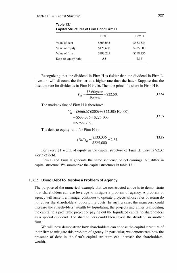
Recognizing that the dividend in Firm H is riskier than the dividend in Firm L,investors will discount the former at a higher rate than the latter. Suppose that thediscount rate for dividends in Firm H is .16. Then the price of a share in Firm H is

(13.6)

The market value of Firm H is therefore:

(13.7)

The debt-to-equity ratio for Firm H is:

(13.8)

For every $1 worth of equity in the capital structure of Firm H, there is $2.37worth of debt.

Firm L and Firm H generate the same sequence of net earnings, but differ incapital structure. We summarize the capital structures in table 13.1.

13.6.2 Using Debt to Resolve a Problem of Agency

The purpose of the numerical example that we constructed above is to demonstratehow shareholders can use leverage to mitigate a problem of agency. A problem ofagency will arise if a manager continues to operate projects whose rates of return donot cover the shareholders’ opportunity costs. In such a case, the managers couldincrease the shareholders’ wealth by liquidating the projects and either reallocatingthe capital to a profitable project or paying out the liquidated capital to shareholdersas a special dividend. The shareholders could then invest the dividend in anotherfirm.

We will now demonstrate how shareholders can choose the capital structure oftheir firm to mitigate this problem of agency. In particular, we demonstrate how thepresence of debt in the firm’s capital structure can increase the shareholders’wealth.

( / )$533.336

$225,0002.37.D E H � �

VH � �

� �

�

($666.67)(800) ($22.50)(10,000)

$533,336 $225,000

$758,3336.

PSL � �$3.60/year

.16/year$22.50.


Table 13.1Capital Structures of Firm L and Firm H

Firm L Firm H

Value of debt $363,635 $533,336

Value of equity $428,600 $225,000

Value of firm $792,235 $758,336

Debt-to-equity ratio .85 2.37

Suppose that a shift in consumer preferences causes each firm’s net annual earningsto decrease from $100,000 to $60,000. Suppose further that it is impracticable toredesign the firms’ products so as to conform to the consumers’ new preferences. Whilethere remains some demand for the firms’ products, the most profitable decision is tocease operations, liquidate the firms, and thus return the capital to the shareholders, whocan then invest it elsewhere. Finally, suppose that the managers of each firm have strongpersonal reasons to continue the current operations. For example, if the firms are liqui-dated, the managers (and their relatives who are now employed by the firm) will have tosearch for new jobs.

How can the shareholders make certain that their managers will liquidate the firmwhenever it is in the shareholders’ interests to do so? The shareholders could ask theirdirectors to order the managers to liquidate the firms. If the directors refuse, the share-holders could elect a new set of directors. But this is not easy to do in the typical firm.In most firms, the directors and the managers own some of the shares themselves. Theownership of the remaining shares is widely dispersed among a large number ofinvestors, each of whom owns a relatively small number of shares. Although eachinvestor would gain wealth if the firm were liquidated, the incentive for any oneinvestor to organize a replacement of the board of directors is usually too small tomake the effort worthwhile.

One solution to this form of the agency problem is to place a sufficiently largeamount of debt in the firm’s capital structure so that the bondholders will force thefirm to liquidate when its earnings no longer cover the shareholders’ opportunitycosts.

The annual net earnings of both Firm L and Firm H have decreased from$100,000 to $60,000. Suppose that if each firm were to liquidate, the bondholders andthe shareholders of that firm could reinvest the capital in a new firm that wouldgenerate annual net earnings of $90,000. Call this new firm Firm N. (Firm N wouldproduce a product that is more profitable than the products that Firms L and H are nowproducing.) Consequently, the investors in each firm have an interest in reallocatinginto Firm N the resources now located in Firms L or H. The bondholders of both firmswould gain because the higher a firm’s (expected) earnings, the less likely it is that adownward fluctuation in those earnings will cause the firm to fail to make thecontractual payments of interest to the bondholders. The shareholders of both firmswould gain because they are residual claimants. For any contractual obligation tothe bondholders, the greater the net earnings, the greater the dividends to theshareholders can be.

The question is, which set of investors is more likely to see their capital reallo-cated to the new, more profitable, firm? It is easy to show that the firm with the greaterdebt-to-equity ratio will provide better protection to its investors.

Since Firm L has 500 bonds outstanding, it must pay its bondholders $40,000 peryear ($80 per bond per year). Firm L’s new annual earnings are $60,000, which willcover this obligation. Since the firm can meet its contractual obligation, the bondhold-ers have no right to force the firm to liquidate. The reduction in Firm L’s annualearnings from $100,000 to $60,000 will be borne entirely by the shareholders becausethey are the residual claimants. After Firm L pays the contractual $40,000 to its bond-holders, only $20,000 will be available for distribution as dividends to shareholders.


Dividends per share in Firm L will now be ($60,000�$40,000)/10,000 shares, or $2 per share. When annual earnings were $100,000, dividends per share were $6 [($100,000�$40,000)/10,000 shares�$6 per share].

When the dividend was $6 per share, investors in Firm L capitalized thissequence of dividends at an annual rate of .14. Consequently, the price per share was($6 per year/.14 per year), or $42.86. If investors use the same discount rate to capital-ize the lower rate of dividends, the new price of a share in Firm L will be ($2 peryear/.14 per year), or $14.29. The decrease in Firm L’s annual net earnings from$100,000 to $60,000, coupled with the fact that Firm L does not use liquidation toallow its investors to reallocate their capital, imposes a capital loss on shareholdersequal to $42.86�$14.29, or $28.57 per share. In percentage terms, the capital loss is$28.57/$42.86, or 66.7%.

The shareholders in Firm H suffer a smaller capital loss than do their counterpartsin Firm L because the high debt-to-equity ratio in Firm H forces that firm to liquidate.

The annual net earnings of Firm H decrease from $100,000 to $60,000, just as isthe case with Firm L. However, the higher debt-to-equity ratio in that firm enables itsbondholders to force the firm to liquidate. Liquidation enables all the investors inFirm H to redeploy their resources into more profitable projects.

Since Firm H has 800 bonds outstanding, it must pay its bondholders $64,000 peryear ($80 per bond per year). Since the firm’s annual earnings are now only $60,000,the bondholders can force a liquidation. For ease of exposition, suppose that the bond-holders and the shareholders of Firm H together redeploy their resources to the newfirm, Firm N, and maintain the same capital structure that they had in Firm H. That is,the bondholders will hold 800 bonds, on each of which Firm N contracts to pay $80per year. The shareholders hold 10,000 shares. We can now calculate the prices of thebonds and the stock issued by Firm N.

Firm N’s total obligation to its bondholders is $64,000 per year, as it was in FirmH. Since the expected annual earnings of Firm N are $90,000, the bondholders canexpect that the firm will be able to meet this obligation. If the bondholders use thesame rate of discount that they did for the bonds of Firm H, the price of each bondissued by Firm N will be ($80 per year/.12 per year)�$666.67.

The dividend per share paid by Firm N will be ($90,000�$64,000)/10,000shares�$2.60 per share. If the shareholders use the same discount rate to capitalizethese dividends that they did for the dividends in Firm H, the price of a share in FirmN will be ($2.60 per year/.16 per year)�$16.25. Consequently, the decrease in theannual net earnings of Firm H from $100,000 to $60,000 will impose on its sharehold-ers a capital loss equal to $22.50�$16.25, or $6.25 per share. The percentage of thecapital loss is $6.25/$22.50, or 27.8%.

Both Firms L and H suffered the same reduction in annual net earnings. Theshareholders in Firm L, who were not able to redeploy their resources, suffered a cap-ital loss equal to 66.7%. By contrast, the shareholders in Firm H suffered a capital lossof only 27.8% because the higher ratio of debt to equity enabled them to overcome theagency problem and redeploy their resources into Firm N.

Of course there are also costs of including debt in the capital structure. In thepreceding example, we saw that the contractual obligation imposed by debt couldbenefit the shareholders by forcing the firm to liquidate when it can no longer cover its


opportunity costs. But in an uncertain and turbulent economic environment, share-holders might be best served by having very small levels of debt (or even no debt) intheir firm’s capital structure. If shareholders believe that their firm’s current difficultyis temporary, while its longer-term prospects are strong, the shareholders might wantto keep the firm intact so as to take advantage of an economic recovery.

As an example, consider the case of a software engineer who has a young familyand who owns a home on which there is a large mortgaged debt. His personal capitalstructure is analogous to that of a firm that has a high debt-to-equity ratio; he has largecontractual obligations in the form of monthly payments to the bank that holds hisdebt. Now suppose that the engineer has just lost his job due to an economic recession.He believes that based on his strong record of productivity it is only a matter of a yearor so before the economy will recover sufficiently for him to be recalled by his formeremployer, or to find a comparable job in the same city. But his personal savings mightnot last long enough to support his family and make monthly payments. His high debt-to-equity ratio might cause him to lose his house before the economy recovers. Thebank is unlikely to allow him to postpone payments on his loan. If the engineer had nomortgaged debt on the house, he could hold on much longer, even if he has to post-pone routine maintenance. (Of course there are some costs, such as property taxes,that cannot be postponed without his eventually losing the house.)

We conclude that there are situations in which a high debt-to-equity ratio will notbe advantageous to the residual claimants, be they shareholders in a firm or the ownerof a house. The optimal debt-to-equity ratio for a firm depends on a variety of circum-stances. Consequently, the simple assertion that debt is bad is false.

In section 13.8, where we discuss the impediments to economic efficiency causedby asymmetric information, we shall discover another disadvantage to a high debt-to-equity ratio.

13.7 A Problem of Agency: Asset Substitution

13.7.1 The Essence of the Problem

In most cases, the earnings of an investment project are stochastic.12 Alternativeprojects differ in the nature of the stochastic processes that generate their earnings. Insome cases, by substituting one investment project for another, a firm can transferwealth from its bondholders to its shareholders. This transfer occurs because thebondholders and the shareholders hold different kinds of claims against the firm’searnings. Specifically, the bondholders hold a contractual claim, while the sharehold-ers hold a residual claim. The managers of the firm serve at the pleasure of the share-holders (to the extent that the directors, whom the shareholders elect, represent theinterests of the shareholders). Therefore, the managers have an incentive to chooseprojects that will maximize the wealth of the shareholders, even if the choice of oneproject over another will reduce the wealth of the bondholders.

Rational and informed investors will anticipate that when a firm sells bonds tofinance a specified new project, there is a risk that the firm will substitute a differentproject in an attempt to transfer wealth from the new bondholders to the shareholders.


To protect themselves against this risk, the investors will reduce the maximal pricethat they are willing to pay for the bonds. To finance any project, a firm has threechoices: use internal funds, use external funds, or use a combination of the two.Internal funds are current or previous earnings that the firm has retained, rather thanpaying as dividends to the shareholders. External funds are monies raised by sellingnew securities. We limit our consideration to stocks and bonds.13 The smaller the por-tion of the project that new investors are willing to finance by purchasing bonds, thelarger the portion that the firm must finance either by selling new shares of stock or byusing retained earnings. If the firm is unwilling or unable to use retained earnings or toissue a sufficient number of new shares, the firm will forego the project, even thoughthe project has a positive net present value. If a firm foregoes a profitable project,there is an inefficient allocation of resources.

In this section, we present a simple numerical example of how bondholders canlose wealth to shareholders through asset substitution and how this transfer of wealthcan cause an inefficient allocation of resources.

13.7.2 Simplifying Assumptions; Definitions

We posit several conditions that will simplify the presentation without destroying theeconomic content. First, the rate of interest on the risk-free asset is equal to zero.Second, the correlation coefficient between the rate of return on each investment proj-ect and the rate of return on the market portfolio is equal to zero, so the value of betafor each project is zero. Therefore, the equilibrium expected rate of return on eachproject is equal to the rate of return on the risk-free asset, which is equal to zero.14

Third, each firm exists for only one period, and undertakes a single project. At t�0,the firm raises the required financing and begins the project. One period later, at t�1,the project generates a value, which the firm immediately distributes to the bondhold-ers and the shareholders. The firm is then liquidated.15

The three foregoing assumptions imply that the market value of the project attime 0 is the expected value of the outcome of the project that will appear at time 1. Ifmarkets are perfectly competitive, the cost of undertaking the project at time 0 will beequal to its expected value.16


Si�The total market values at t�0 of the stockholders’ claims to the earnings ofProject i

Bi�The total market values at t�0 of the bondholders’ claims to the earnings ofProject i

Vi�Si�Bi�The total market at t�0 of the value of Project iF�The aggregate face value of the bondsBi�Minimum (F, Vi)Si�Maximum (Vi�F, 0)

The bond is a contractual claim that requires the firm to pay F to the bondholders. Ifthe value of the firm at t�1 is less than the firm’s obligation to the bondholders (V1F),the firm must pay the entire value of the firm to the bondholders. Hence, the market valueof the bonds at t�1 is the minimum of F and V1.


The shareholders hold a residual claim. At t�1, the market value of their claim is whatever value remains in the firm after the firm meets its obligation to thebondholders. Therefore, the market value of the stock at t�1 is the maximum ofV1�F and 0.

13.7.3 A General Example of an Investment Project

In this section, we present a simple, general example of an investment project. In thefollowing section, we use this general example as a template to analyze four specificnumerical examples of the problem of asset substitution.

The firm begins the project at t�0. One period later, at t�1, the firm liquidatesthe project and receives X. The liquidation value X is a random variable governed by auniform probability density function over the interval (L, U ), in which L and U areconstants that are constrained by 0�LU. The probability density for the randomvariable X is 1/(U�L). Let X0 and X1 be possible values for X, with X0X1. Then theprobability that X will take a value in the interval (X0, X1) is (X1�X0)/(U�L). Using auniform density function for the outcome of the investment project makes the calcula-tions easier without making the example vacuous.17

For the numerical examples in the following section, we use the followingformulas; the derivations of these formulas are in the appendix to this chapter.

The expected value of X, E(X), is equal to (L�U)/2, which is the midpoint of therange of possible values for X.

The standard deviation of X is equal to (U�L)2/2√3.The value at t�0 of the shareholders’ claim to the earnings of the project is

S�(U�F)2/2(U�L).The value at t�0 of the bondholders’ claim, B, to the earnings of the project is the

difference between the expected value of the project and the value of the shareholders’claim. That is, B�E(X)�S.

13.7.4 Three Numerical Examples of Asset Substitution

We now examine three numerical examples using the general template presented in thepreceding section. The examples differ in the values for L and U, the lower and upperboundaries of the probability density function for the project. We have drawn the proba-bility density functions for four projects in figure 13.1. For each project, we indicate thevalues for L, U, the expected value, and the standard deviation. We compare these valuesin table 13.2. The details of the calculations appear in the appendix to this chapter.

We can illustrate the problem of asset substitution by comparing Projects B, C,and D separately with Project A. Suppose that the firm, acting for its shareholders,announces that it will undertake Project A, and that it will finance that project by sell-ing bonds that have a face value of $90. Investors who purchase the bonds at time 0will receive a payment at time 1 that will depend on the outcome of a random variable.The market value of the bonds at time 0 is the expected value of the payments that thebondholders will receive at time 1. If investors believe that the firm will, in fact,undertake Project A, the market value of the bonds at time 0 will be $82. The cost ofundertaking Project A is the market value (at time 0) of that project, which is $100.


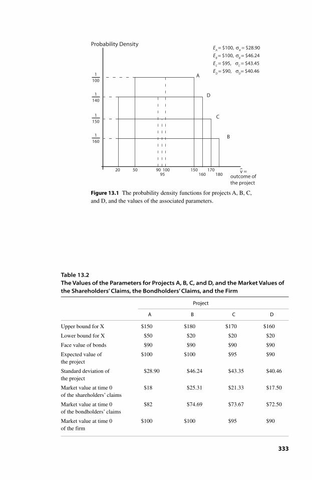
333

Figure 13.1 The probability density functions for projects A, B, C,and D, and the values of the associated parameters.

v =

Probability Density

outcome of the project

A

D

C

B

20 50 10095

90 150160

170180

EC

= $95, σC

= $43.45

EB

= $100, σB

= $46.24

ED

= $90, σD= $40.46

EA

= $100, σA

= $28.90

1100

1140

1150

1160

Table 13.2The Values of the Parameters for Projects A, B, C, and D, and the Market Values ofthe Shareholders’ Claims, the Bondholders’ Claims, and the Firm

Project

A B C D

Upper bound for X $150 $180 $170 $160

Lower bound for X $50 $20 $20 $20

Face value of bonds $90 $90 $90 $90

Expected value of $100 $100 $95 $90the project

Standard deviation of $28.90 $46.24 $43.35 $40.46the project

Market value at time 0 $18 $25.31 $21.33 $17.50of the shareholders’ claims

Market value at time 0 $82 $74.69 $73.67 $72.50of the bondholders’ claims

Market value at time 0 $100 $100 $95 $90of the firm

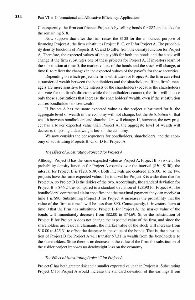
Consequently, the firm can finance Project A by selling bonds for $82 and stocks forthe remaining $18.

Now suppose that after the firm raises the $100 for the announced purpose offinancing Project A, the firm substitutes Project B, C, or D for Project A. The probabil-ity density functions of Projects B, C, and D differ from the density function for ProjectA. Therefore, the expected values of the payoffs for both the bonds and the stock willchange if the firm substitutes one of these projects for Project A. If investors learn ofthe substitution at time 0, the market values of the bonds and the stock will change, attime 0, to reflect the changes in the expected values of the payoffs for those securities.

Depending on which project the firm substitutes for Project A, the firm can effecta transfer of wealth between the bondholders and the shareholders. If the firm’s man-agers are more sensitive to the interests of the shareholders (because the shareholderscan vote for the firm’s directors while the bondholders cannot), the firm will chooseonly those substitutions that increase the shareholders’ wealth, even if the substitutioncauses bondholders to lose wealth.

If Project A has the same expected value as the project substituted for it, theaggregate level of wealth in the economy will not change; but the distribution of thatwealth between bondholders and shareholders will change. If, however, the new proj-ect has a lower expected value than Project A, the aggregate level of wealth willdecrease, imposing a deadweight loss on the economy.

We now consider the consequences for bondholders, shareholders, and the econ-omy of substituting Projects B, C, or D for Project A.

The Effect of Substituting Project B for Project A

Although Project B has the same expected value as Project A, Project B is riskier. Theprobability density function for Project A extends over the interval ($50, $150); theinterval for Project B is ($20, $180). Both intervals are centered at $100, so the twoprojects have the same expected value. The interval for Project B is wider than that forProject A, so Project B is the riskier of the two. Accordingly, the standard deviation forProject B is $46.24, as compared to a standard deviation of $28.90 for Project A. Thebondholders’ contractual claim specifies that the maximal payment they can receive attime 1 is $90. Substituting Project B for Project A increases the probability that thevalue of the firm at time 1 will be less than $90. Consequently, if investors learn attime 0 that the firm has substituted Project B for Project A, the market value of thebonds will immediately decrease from $82.00 to $74.69. Since the substitution ofProject B for Project A does not change the expected value of the firm, and since theshareholders are residual claimants, the market value of the stock will increase from$18.00 to $25.31 to offset the decrease in the value of the bonds. That is, the substitu-tion of Project B for Project A will transfer $7.31 in wealth from the bondholders tothe shareholders. Since there is no decrease in the value of the firm, the substitution ofthe riskier project imposes no deadweight loss on the economy.

The Effect of Substituting Project C for Project A

Project C has both greater risk and a smaller expected value than Project A. SubstitutingProject C for Project A would increase the standard deviation of the earnings (from


$28.90 to $43.35), and reduce the expected value (from $100 to $95). Comparing thecolumns for Projects A and C in table 13.2 indicates that substituting Project B forProject A will decrease the market value of the bonds (from $82.00 to $73.67) andincrease the value of the stock (from $18.00 to $21.33). Bondholders lose $8.33(because they absorb the entire reduction of the firm’s $5.00) and lose an additional$3.33 in wealth transferred to the shareholders. Substituting Project C for Project Atransfers wealth from the bondholders to the shareholders and imposes a deadweightloss on the economy.

The Effect of Substituting Project D for Project A

Project D, like Project C, has both greater risk and a smaller expected value thanProject A. Unlike Project C, however, substituting Project D for Project A will reducethe wealth of both the bondholders and the shareholders, and impose a deadweightloss of $10 ($100�$90) on the economy. The bondholders would lose $9.50($82.00�$72.50); the shareholders would lose $0.50 ($18.00�$17.50).

We conclude from the preceding numerical examples that if the firm can raise $82from bondholders by announcing an intention to undertake Project A, the firm cantransfer wealth from the bondholders to the shareholders by substituting Project B forProject A. The economy will incur no deadweight loss because Projects A and B havethe same expected value. If Project B is not available, the firm could still transferwealth to its shareholders by substituting Project C for Project A. In this case, theeconomy would incur a deadweight loss of $5.00. The firm would not substituteProject D for Project A; to do so would cause the shareholders to lose wealth.

Rational investors will recognize that the firm can transfer wealth from bondhold-ers to shareholders by substituting Project B for Project A. Unless the firm can guar-antee that it will undertake Project A, prospective bondholders will anticipate that theywill have a contractual claim on the earnings of Project B and thus pay no more than$74.69 for the bonds. Consequently, to finance Project B, the firm will have to use$25.31 of retained earnings, or raise that amount from shareholders.

If Project B is not available, prospective bondholders will anticipate that the firmwill substitute Project C for Project A and thus will pay only $73.67 for the bonds.Consequently, to finance Project C, the firm must either use $26.33 of retained earnings,or raise that amount in new capital from the shareholders. The economy will incur adeadweight loss equal to the difference between the expected values of Projects A and C.

Notice that the firm has no incentive to protect the economy from the deadweightloss created by undertaking Project C rather than Project A. To do so would impose aloss on the shareholders. Anticipating that the firm will proceed with Project C, thebondholders will contribute only $73.67 in new capital to the firm. Since the cost ofProject A is its expected value, $100, the firm would either have to contribute $26.33($100.00�$73.67) from retained earnings, or raise $26.33 in new capital from theshareholders. But if the firm undertakes Project A, the market value of the sharehold-ers’ claims will decrease from $26.33 to $18.00, while the value of the bondholders’claim will increase from $73.67 to $82.00. The economy will avoid the deadweightloss of the difference between the expected values of Projects A and C, but there willbe a transfer of wealth from the bondholders to the shareholders.


13.7.5 Mitigating the Inefficient Allocation by Using Restrictive Covenants

Firms and investors can avoid the inefficient allocation of resources that can occurfrom the substitution of riskier projects for less risky ones by writing, and accepting,restrictive covenants in the bonds. A restrictive covenant is a provision in the bondthat restricts the firm to use the funds provided by the bondholders only for a specificproject.

For example, suppose that the ES&D Railroad offers to sell bonds to finance thepurchase of freight cars to be used only on the route between Cleveland and Boston.The railroad also has a route between Kansas City and Baltimore. The returns for thetwo routes are governed by different probability density functions. The expectedvalue for the route between Kansas City and Baltimore is less than the expectedvalue for the route between Cleveland and Boston, and the risk for the route betweenKansas City and Baltimore is higher than the risk for the route between Clevelandand Boston. Under some conditions, the railroad will have an incentive to sell bondsto finance the purchase of freight cars for the route between Cleveland and Boston,and then use the cars on the route between Kansas City and Baltimore. Anticipatingthis, the bondholders will not pay as much for the bonds as they would if they couldbe certain that the railroad would use the new cars only on the route betweenCleveland and Boston.

The railroad could avoid this problem by including a restrictive covenant in thebonds. The covenant would state that each new car would be identified by a serialnumber, permanently stamped into the frame of the car when it was built. Further,each car would be dedicated to service on the route between Cleveland and Boston. Touse the car on any other route would be a default by the railroad. A default wouldtransfer to the bondholders certain rights formerly assigned to the shareholders.18

13.8 Economic Inefficiencies Created by Asymmetric Information

Economists use the term asymmetric information to describe a situation in which theactors on one side of a market have better information about relevant future outcomesthan the actors on the other side of the market do. There are numerous situations inwhich asymmetric information can create an inefficient allocation of resources.Consider the following example.19

It is not unusual for the managers of a firm to have better information about thefirm’s ability to generate earnings than the current shareholders or prospective newinvestors do. In particular, the managers might have superior information about aproposed new investment project. If the firm lacks sufficient internal funds to financethe new project, the firm must raise additional capital by selling new securities. Thefirm’s managers and the prospective new investors who could buy the new securitiesare on opposite sides of the market. In this section, we demonstrate that if the asym-metry of information between the managers and the prospective new investors is suf-ficiently severe (in a sense that we define below), the firm will forego the projecteven though the project has a positive net present value. Clearly, this outcome is


economically inefficient. We also demonstrate how a firm, again under some condi-tions, can overcome the effects of the asymmetric information by issuing a sophisti-cated kind of security. The purpose of this demonstration is to show a relationshipbetween economic efficiency and the capital structures of firms.

13.8.1 A Brief Summary of Akerlof’s Market for Lemons

The seminal paper on asymmetric information presented in 1970 by George Akerlof isthe basis of many advances in economics.20 Akerlof demonstrated that asymmetricinformation can cause a market to collapse, thereby precluding some mutually benefi-cial exchanges that would occur if the asymmetry were eliminated. In section 2.4.1 ofchapter 2 we presented in some detail a simple version of Akerlof’s model, and in sec-tion 2.4.2 we used Akerlof’s model to demonstrate how asymmetric informationbetween managers of firms and prospective investors could create an inefficient allo-cation of resources. We now summarize briefly our work in chapter 2 on asymmetricinformation, and then consider a more sophisticated analysis that involves bonds thatare callable and convertible.

The usual introduction to Akerlof’s model is to consider a market for usedautomobiles. There is a set of automobiles that are individually offered for sale. Eachautomobile has a certain quality, such as the number of miles of service that it willdeliver per $100 of expenditure for maintenance and repair. The current owner of eachautomobile knows the quality of that automobile. Prospective buyers of the automo-biles know only the probability distribution of the values of quality across the set ofautomobiles offered for sale. Thus, there is asymmetric information in the market forused automobiles; the prospective sellers have superior information relative to theprospective buyers.

The asymmetry of information between buyers and sellers creates an asymmetryof optimal behavior for buyers and sellers. The maximal price that a rational buyerwill pay for any automobile depends on the average quality of the automobiles offeredfor sale.21 On the other side of the market, the minimal price that a rational seller willaccept for a particular automobile depends on the quality of that automobile.Consequently, owners of used automobiles will not offer for sale any automobile thathas a level of quality greater than the average level of quality across the population ofused automobiles. Rational buyers, knowing that sellers will withhold all the high-quality automobiles, will revise downward the maximal price that they will offer for aused automobile. The reduction in the price offered by buyers will cause owners towithhold even more automobiles, which will cause buyers to reduce further the maxi-mal price that they will pay. This process is degenerative. In the end, the marketcollapses; no used automobiles are offered for sale.

The asymmetry of information between sellers and buyers creates an inefficientallocation of resources. Presumably, there are some current owners of automobiles forwhom the marginal values of (retaining) those automobiles is less than the marginalvalues that some prospective buyers would place on (acquiring) those automobiles. Ifthere were no asymmetry of information, some current owners and some prospectivebuyers could effect mutually beneficial exchanges.


In section 2.4.2, we used a simple version of Akerlof’s model to demonstrate howasymmetric information between managers of firms and prospective investors couldcreate an inefficient allocation of resources. We considered a population of firms.Each firm is either strong or weak. Only the managers of a firm know whether thatfirm is strong or weak. A strong firm has a larger net present value for its current oper-ations than does a weak firm. Each firm has an opportunity to undertake a profitablenew investment project, but only if the firm can finance that project by selling newshares of stock. The net present value of the project for a strong firm is greater than fora weak firm. The cost of undertaking the project is the same for each type of firm.

Prospective investors, who could finance the project in either type of firm, knowthe net present values of the current operations and the new project in each type of firm.Unfortunately, the investors cannot determine whether a particular firm is strong orweak. Consequently, if a firm attempts to raise capital to finance the new project, themaximal price that investors will pay for those shares depends on the average of the netpresent values of strong firms and weak firms, including the new project, with the twonet present values weighted by the numbers of each type of firm in the total populationof firms. That is, prospective investors regard each firm that offers to sell new shares asa random draw from a population that contains both strong and weak firms.

To recover their opportunity costs for financing the new project, the newinvestors must acquire a certain proportion of the ownership of the firm. The currentshareholders in a firm retain the remaining proportion of the firm. The proportion thatthe investors must acquire of a strong firm is smaller than the proportion that theymust acquire of a weak firm. From the perspective of a strong firm, the presence ofweak firms contaminates the pool of firms. Because investors regard any firm as if itwere a weighted average of a strong firm and a weak firm, the proportion of a strongfirm that the new investors acquire is larger than it would be if the managers of thestrong firm could credibly inform the new investors that they are, in fact, acquiring astrong firm.

Depending on the net present values of the two types of firms, with and without thenew project, and on the cost of the project, the shareholders of a strong firm will foregothe project because the new investors would acquire so large a proportion of the firmthat the current shareholders would lose wealth. By definition, if a project has a positivenet present value, the sequence of payments generated by that project will cover morethan the opportunity costs of financing it. Therefore, it is possible for both the currentshareholders and the new investors to gain wealth if the firm undertakes the project, butonly if the new investors do not acquire too large a proportion of the firm. If the weakfirms are sufficiently numerous in the population of firms, and if each firm must financethe project by selling new shares, the current shareholders of a strong firm will foregothe project, thereby creating an inefficient allocation of resources.

13.8.2 A Numerical Example in Which There Is Symmetric Informationbetween Managers and Investors

For comparison, we first present an example in which there is symmetric informationbetween the managers of a firm and new investors who are being asked to finance anew project.


There are 10,000 firms in a particular industry. Each firm has only common stockoutstanding. The price of one share of a firm’s common stock is the present value ofthat firm’s future sequence of earnings per share. The market value of a firm is equalto the price of its stock multiplied by the number of shares outstanding. Therefore, themarket value of a firm is the present value of its future earnings.

Among the 10,000 firms are 1,000 strong firms and 9,000 weak firms. Themarket value of a strong firm is $600; the market value of a weak firm is only $100.Since there is no asymmetric information, all investors can determine with certaintywhether a particular firm is strong or weak.

Each firm has an opportunity to invest in a new project. The cost of undertakingthe project for any firm is $50. The net present value of the project in a strong firm is$80. In a weak firm, the net present value of the project is only $30. No firm has anyexcess internal funds with which to finance the project. Consequently, if a firm wantsto undertake the project, it must sell new securities in a quantity sufficient to raise $50.

If a strong firm undertakes the project, the market value of that firm will increasefrom $600 to $730. The increase of $130 in market value consists of the $50 of addi-tional capital that the firm raises to finance the project, plus $80 for the net presentvalue of the project.22 If a weak firm undertakes the project, the market value of thatfirm will increase from $100 to only $180. The increase of $80 includes the $50 worthof resources required to finance the project plus the net present value of the project,which is only $30 for a weak firm.

To finance the project, each firm must sell new shares in a quantity sufficient toraise $50. The number of new shares that a firm must sell to raise $50 determines theproportion of the firm that the new investors will acquire. Competition amonginvestors will ensure that the proportion of a firm that the investors will acquire willbe such that the new investors will recover only their opportunity costs. The greaterthe market value of the firm for which the new investors are providing the $50, thesmaller is the proportion of that firm that the new investors must acquire to recovertheir opportunity costs. Since investors can distinguish with certainty between strongfirms and weak firms, a strong firm can raise the $50 by granting a smaller proportionof the firm to new investors than a weak firm can. We can demonstrate this easilyusing the numerical characteristics of the two kinds of firms.

The market value of a strong firm including the new project is $730. If newinvestors finance the project by purchasing $50 of new shares, then the proportion ofa strong firm that the new investors will own is $50/$730�.068 (after rounding).Assume (only for simplicity) that the rate of interest at a bank is equal to zero. Thenthe new investors need to recover only $50 to meet their opportunity costs. If the inter-est rate is zero, the value of the new investors’ shares next period will be $50, and thevalue of the firm next period will be $730. Then the new investors can sell their sharesnext period and recover their investment (including zero opportunity costs).

If a strong firm can finance the project by ceding only .068 of the firm to the newinvestors, the current shareholders will retain the proportion 1.000�.068, or .932, ofthe firm. Including the new project, the market value of the strong firm is $730. Thenthe value of the current investors’ holdings will be (.932)$730, or $680 approximately.The market value of the value of a strong firm without the new project is $600. Thenet present value of the new project in a strong firm is $80. Consequently, the current


shareholders capture the full net present value of the new project. The new investorsobtain only .068 of the firm in exchange for purchasing $50 worth of new shares.Since (.068)$730�$49, we conclude (after rounding) that the new investors recoveronly their opportunity costs.23

We have demonstrated that if a strong firm finances the project by selling newshares, the current shareholders obtain the entire net present value of the new project,while the new investors recover only their opportunity costs. The same result holds fora weak firm.

Including the new project, the market value of a weak firm is $180. The proportionof a weak firm acquired by new investors is $50/$180�.278. Consequently, the currentshareholders retain 1.000�.278, or .722 of the firm. Once the weak firm undertakes theproject, the wealth of the current shareholders increases from (1.000)$100 to(.722)$180, which is equal to $129.96, or $130 after rounding. The wealth of the cur-rent shareholders increases by $30, which is the full net present value of the project ina weak firm. The new investors recover only their opportunity costs.

13.8.3 A Numerical Example in Which There Is Asymmetric Informationbetween Managers and Investors

We now modify the example of the preceding section by dropping the assumption thatinvestors can distinguish between strong firms and weak firms with certainty.Consider first the situation before any firm undertakes the new project. As before,there are 1,000 strong firms and 9,000 weak firms. The market value of a strong firmis $600, and the market value of a weak firm is $100. Only the managers of a firmknow whether their firm is strong or weak. Therefore, if a group of investors were topurchase a single firm, they would have a 90% chance of obtaining a weak firm andonly a 10% chance of obtaining a strong firm. If the investors were to purchase 100 ofthese firms, the average value of the firms that they purchase would be equal to(.9)($100)�(.1)($600), or $90�$60, or $150.24 Since only the managers knowwhether a particular firm is strong or weak, the maximal price that the investorsshould pay for a firm is $150.

We will now determine whether a firm should undertake the new project if the firmmust finance that project by selling new shares. The answer depends on: (1) the differ-ence in the market values of the strong firms and the weak firms without the project, (2)the difference in net present values of the project in the two kinds of firms, (3) theamount of new capital that a firm must raise to finance the project, and (4) the ratio ofstrong to weak firms in the population of firms.

The market value of a strong firm that undertakes the project is $730. The marketvalue of a weak firm that undertakes the project is $180. If all firms undertake theproject, the average market value of the firms will be (.90)($180)�(.10)($730), or$235. If new investors purchase $50 worth of new shares in each firm, the investorsmust acquire at least $50/$235, or .213 (after rounding) of each firm in order torecover their opportunity costs. Competition among investors will ensure that eachfirm can raise the $50 required to finance the new project by selling a quantity of new


shares that will allow the new investors to acquire .213 of the firm. Consequently, thecurrent shareholders will retain .787 of the firm.

When investors cannot determine whether a given firm is strong or weak, a strongfirm should not undertake the new project. If a strong firm undertakes the project, thevalue of the current shareholders’ stake will be (.787)($730), or $574.51. Without thenew project, the market value of the strong firm is $600, all of which is retained by thecurrent shareholders because, without the new project, there are no new shareholders.Clearly, the current shareholders in a strong firm lose wealth if their firm sells newshares to undertake the project. Selling new shares to finance the project will transfer$600�$574.51, or $25.49 in wealth from the current shareholders to the newshareholders.

To see this another way, consider the situation of the new shareholders who werefortunate enough to have drawn a strong firm in which to invest. The new shareholdersacquire .213 of the firm. Since the market value of the strong firm with the project is$730, the value of the new investors’ stake is (.213)($730), or $157.62. We can write$157.62 as $50�$80�$27.62. The value of the new investors’ stake in the strong firm allows them to recover their opportunity costs ($50), capture the entire netpresent value of the project ($80), and receive a transfer of $27.62 from the currentshareholders.

The current shareholders in a strong firm will lose wealth to the new shareholdersbecause the number of strong firms in the population of all firms is so low that theaverage market value of a firm is much closer to the market value of a weak firm thanto a strong firm ($235 is much closer to $180 than it is to $730). The smaller theproportion of strong firms, the lower will be the average market value of a firm withthe project relative to the market value of a strong firm with the project. The lower theaverage market value of a firm with the project, the higher the proportion of a firm thatthe new investors must acquire if they are to recover their opportunity costs. In thepresent example, the proportion of strong firms is so low, and consequently the pro-portion of each firm that the new investors must acquire is so large, that those newinvestors fortunate enough to invest in a strong firm receive a transfer of wealth fromthe current shareholders.

We now consider whether a weak firm should finance the project by selling new shares. If a weak firm sells new shares, the current shareholders will retain(1.000�.213) or .787 of the firm, just as in the case of a strong firm. The market valueof a weak firm that undertakes the project is $180. Consequently, the value of the newinvestors’ stake in a weak firm that undertakes the project will be (.213)$180, or$38.34. This is less than the new investors’ opportunity cost, which is $50. Hence, thenew investors suffer a loss equal to $50�$38.34, or $11.66. It is easy to show that the$11.66 is transferred from the new investors to the current shareholders.

When a weak firm sells new shares to raise the $50 for the project, the value ofthe current investors’ stake in the firm will increase from (1.000)$100 to (.787)($180),or from $100 to $141.66. We can disaggregate this by writing $141.66�$100�

$30�$11.66. The value of the current shareholders’ claim increases by the full netpresent value of the project ($30) plus $11.66 in wealth transferred from the newinvestors.


13.8.4 The Collapse of the Market

In the preceding numerical example, there are net transfers of wealth between thecurrent shareholders of a firm and the investors who finance the project. In strongfirms, the new investors gain at the expense of the current shareholders. In weakfirms, the current shareholders gain at the expense of the new investors. In each case,the transfers occur because the asymmetry of information between managers of firmsand investors prevents the new investors from acquiring a proportion of the firm thatwill allow them to cover no more than their opportunity costs and no less. In ourexample, the new investors acquire .213 of the firm, whether the firm is strong orweak. For a strong firm, this proportion is large enough to effect a transfer of wealthfrom the current shareholders to the new investors. But for a weak firm, the proportion.213 is small enough to effect a transfer of wealth in the opposite direction, from thenew investors to the current shareholders.

Since neither strong firms nor weak firms can finance the project by selling newlycreated shares without causing net transfers of wealth, the market for new securitieswill collapse. A market is a mechanism through which individuals can effect mutuallybeneficial exchanges. But in the example at hand, one party or the other always suffersa net loss of wealth. Consequently, unless the asymmetry of information betweenmanagers and investors is eliminated, neither strong firms nor weak firms will be ableto finance the new project by selling new shares.

We will now demonstrate that the asymmetry of information will disappearbecause all investors know that only weak firms will attempt to sell new shares.Competition among investors will enable each weak firm to raise $50 from newinvestors by allowing them to acquire the proportion $50/$180, or .278, of the firm.The current shareholders will retain the proportion 1.000�.278, or .722, of the firm.The new project increases the market value of the firm from $100 to $180.Consequently, the market value of the current shareholders’ stake in the firm increasesfrom (1.000)$100 to (.722)$180, or from $100 to (approximately) $130. The currentshareholders capture the entire net present value of the project, leaving the newinvestors to recover only their opportunity costs.

13.8.5 Economic Inefficiency Caused by Asymmetric Information

Recall from earlier chapters that an efficient allocation of resources requires that everypotential for a mutually beneficial exchange is realized. In particular, every firm mustundertake any investment project that has a positive net present value. In principle, thenet present value of the project can be distributed across various parties in a way thatallows at least one of the parties to gain wealth without imposing a loss on any party.That is, there need be no net transfer of wealth.

In the numerical example at hand, the net present value of the new project ispositive in both weak firms and strong firms. Therefore, there will be an inefficientallocation of resources unless both kinds of firms undertake the project. But theasymmetric information between managers and investors permits only the weak firmsto finance the project by selling new shares. Consequently, if a strong firm has noaccess to financing other than by selling new shares, that firm must forego the


project. In this case, the asymmetric information creates an inefficient allocation ofresources.

The shareholders of a strong firm would lose wealth to the new investors if thefirm undertakes the project because the new investors would acquire too large aproportion of the firm. The ratio of weak firms to strong firms is so large that the aver-age market value of a firm is too close to the market value of a weak firm. The weakfirms contaminate the pool of firms from which the investors will draw when purchas-ing new securities. If the managers of each strong firm could credibly signal the qual-ity of their firm to potential new investors, there would be no need to grant so large aproportion of the firm to the new investors in exchange for their financing the project.Knowing that they were acquiring a portion of a strong firm, the new investors wouldrecognize that they could accept a smaller proportion of that firm and still recovertheir opportunity costs.

13.8.6 Using Callable, Convertible Bonds to Eliminate EconomicInefficiencies Caused by Asymmetric Information

We will now show how a strong firm can overcome the problem of asymmetric infor-mation if either type of firm can choose between issuing straight equity or issuingcallable, convertible bonds to finance the project. Investors know the level of earningsthat a strong firm can generate, both with and without the new project. Consequently,investors know how a strong firm’s decision on how to finance the project will affectthe wealth of that firm’s current shareholders. Similarly, investors can predict how aweak firm’s decision on how to finance the project will affect the wealth of that firm’scurrent shareholders. Under some conditions, the managers of strong firms can set theterms of a callable, convertible bond so that investors will recognize that only a strongfirm can use that security to finance the new project without imposing a loss of wealthon its current shareholders. Similarly, the managers of weak firms can set the terms ofan offering of straight equity so that investors will recognize that only a weak firm canuse that security to finance the project without imposing a loss on its current share-holders. Consequently, the managers of any firm can credibly distinguish their firm asstrong or weak by their choice of how to finance the project.

Each firm’s choice of which security to issue eliminates the asymmetry of infor-mation between managers of firms and investors who can finance the new project.Consequently, each firm is able to finance the new project without imposing net trans-fers of wealth between current shareholders and new investors. Economists call thisoutcome a separating equilibrium because, with the asymmetry of information elimi-nated, investors are able to separate strong firms from weak firms before committingfunds to finance the firms’ projects. In the preceding section, the presence of asym-metric information required investors to evaluate each firm as if it were a weightedaverage of a pool of weak firms and strong firms. Economists call this outcome apooled equilibrium.

Following is a numerical example of how the managers of weak firms and themanagers of strong firms can use their choice of securities to create a separating equi-librium in which both types of firms can attract additional capital from new investorsto finance profitable projects.


Assume that the risk-free rate of interest is equal to zero. Assume also that theearnings of all firms are uncorrelated with the earnings of the macroeconomy; henceeach firm’s value of beta is equal to zero. These assumptions will simplify our calcu-lations without affecting the fundamental principles of the separating equilibrium thatwe want to present.

The current value of the strong firm’s assets is $600. The current value of theweak firm’s assets is $100. At the moment, each firm has only common stock out-standing. Each firm has an opportunity to begin a new project at a cost of $50. Neitherfirm has any idle cash, so a firm that wants to undertake the project must raise $50 innew capital. The net present value of the project in a strong firm is $80; the net pres-ent value of the project in a weak firm is only $30. Since the net present values of theproject are positive in both types of firms, it is possible, in principle, for each firm toconstruct a mutually beneficial exchange between its current shareholders and a set ofnew investors. We can easily calculate the bounds on the values of the claims of thenew investors that will create a mutually beneficial exchange.

The market value of a strong firm that undertakes the project is $730, of which$600 is the value of the strong firm’s current assets, $50 is the value of the new capi-tal, and $80 is the net present value of the project in a strong firm. The new investorswho provide the $50 of additional capital required to finance the project must obtain aclaim against that firm that is worth more than $50 and less than $130. If the newinvestors are to gain wealth, they must obtain a claim that is worth more than $50.(Recall that the interest rate is equal to zero.) If the current shareholders are to gainwealth, the value of the new investors’ claim must be less than $130. Otherwise, thevalue of the current shareholders’ claim will be worth less than $600, which is theirwealth without the project.

For a weak firm, the value of the firm with the project is $180, of which $100 isthe value of that firm without the project, $50 is the new capital required to finance theproject, and $30 is the net present value of the project in a weak firm. Proceeding aswe did for the strong firm, we find that both the current shareholders and the newinvestors will gain wealth if the value of the new investors’ claim exceeds $50 and isless than $80.

We can now show that a strong firm can effect a mutually beneficial exchangebetween its current shareholders and new investors by financing the project with acallable, convertible bond, and a weak firm can effect a similar exchange by usingstraight equity to finance the project. By knowing the characteristics of a strong firm,investors will infer (correctly) that a strong firm can use the bond to increase the wealthof its current shareholders, while allowing the new investors to gain wealth also.Similarly, investors will recognize that a weak firm can use straight equity to increaseits current shareholders’ wealth, again allowing the new investors also to gain wealth.More important, investors will recognize that neither type of firm will masquerade asthe other type of firm by issuing the security associated with that type of firm. To do sowould cause the current shareholders in the “masquerading” firm to lose wealth.

Events occur at time 0 and time 1. At time 0, each kind of firm has an opportunityto undertake the new project. At time 1, all investors learn which of the firms arestrong and which are weak. Any firm that issued a bond at time 0 must pay the facevalue of that bond to whoever holds the bond at time 1.


There are two securities that a firm can issue at time 0 to finance the project. Thefirst security is a bond that has a face value of $125, is callable (by the issuing firm)for $110, and is convertible (by the bondholders) into .16 of the equity of the firm. Thesecond security is straight equity that represents .28 of the firm. We will now examinethe effects on the wealth of current shareholders and the wealth of new investors forthe several cases distinguished by the type of firm, the firm’s choice of which securityto issue, and the choices made by managers and investors with respect to calling andconverting the bond.

Consider first what will happen if the strong firm issues the bond at time 0. Attime 1, the bondholders (and everyone else) learn that the firm in which they hold thebond is a strong firm. The market value at time 1 of a strong firm that undertook theproject is $730. The firm now must decide whether to call the bond.

If the firm calls the bond, the bondholders have a choice. They can accept the call,in which case they surrender the bond in exchange for a payment of the call price, whichis $110. The bondholders’ alternative is to convert their bond into equity. By convertingto equity, the bondholders will acquire .16 of the firm. Since the market value of the firmat time 1 is known by everyone to be $730, the bondholders recognize that if they con-vert their bond into equity, the value of their position will be equal to (.16)$730, or$116.80. So in the event that the firm calls the bond, the bondholders will convert toequity, because the value of the converted bond ($116.80) exceeds the call value of thebond ($110). We say that the managers of the strong firms can force conversion of thebond at time 1 because the converted value of the bond exceeds the call price.

Since the value of the converted bond, $116.80, exceeds what the new investorspaid for the bond, $50, the new investors will gain an increase in wealth equal to$116.80�$50, or $66.80. Since the new investors will have acquired .16 of the equityin the strong firm, the original shareholders will have retained the proportion1.00�.16, or .84 of the firm. Then the value of the original shareholders’ claim is(.84)$730, or $613.20. Had the firm declined the project, the original shareholders ofthe strong firm would have owned 100% of a firm worth $600. Therefore, if the strongfirm undertakes the project, finances it by issuing a callable, convertible bond, andforces conversion of the bond, the original shareholders will increase their wealth by(.84) $730�(1.00)$600, or $613.20�$600.00, or $13.20. Both the original sharehold-ers and the new investors gain wealth, so the firm will have effected a mutually bene-ficial exchange. Moreover, the sum of the gains in wealth of the original shareholdersand the new investors is $13.20�$66.80, or $80, which is the net present value of theproject in a strong firm. Therefore, the net present value of the project is fully distrib-uted between the original shareholders and the new investors.

In earlier chapters, we showed that in the absence of uncertainty and asymmetricinformation, the original shareholders capture the entire net present value of theproject, and the new investors only cover their opportunity costs. In the present exam-ple, the original shareholders do not capture the entire net present value; in fact thenew investors gain more wealth than the original shareholders do. Nevertheless, thefirm does invest in the project, and each party does gain wealth. Therefore, we have anefficient allocation of resources.

We next examine what happens if the strong firm does not call the bond. If thestrong firm does not call the bond at time 1, the bondholders may still choose to convert


their bond to .16 of the equity in the firm. The value of the converted bond is (.16)$730,or $116.80. The bondholders’ alternative is to hold the bond and receive its face value,which the firm must pay at time 1. Since the total value of the strong firm with the proj-ect is $730, the value of the original shareholders’ claim will be $730�$125, or $605.But we showed above that if the firm forces conversion of the bond by calling it, thevalue of the original shareholders’ claim will be equal to $613.20. Since $613.20�$605,we conclude that the firm will force conversion of the bond by calling it.

We next show that a weak firm will not offer the bond. Suppose that a weak firmdoes offer the bond at time 0 and does not call that bond at time 1. At time 1, everyonewill learn that the firm is a weak firm, whose market value with the project is $180. Ifthe firm does not call the bond, the bondholders can choose between converting theirbond into the proportion .16 of the equity of the firm, or accepting the face value ofthe bond. If the bondholders convert, the value of their equity will be (.16)$180, or$28.80. If the bondholders do not convert, the firm must pay the bondholders $125.Clearly, if the firm does not call the bond, the bondholders will not convert becausethe face value of the bond exceeds its converted value. If the weak firm does not callthe bond, the new investors will obtain $125, for a net gain in wealth equal to$125�$50, or $75. Since the total value of the weak firm is $180, the value of theoriginal shareholders’ claim will be $180�$125, or only $55. If the weak firm haddeclined the new project, the original shareholders would have had a claim worth(1.00)$100, or $100.

We conclude that if a weak firm finances the project by selling a bond at time 0,and does not call that bond at time 1, the new investors will gain $75, and the originalshareholders will lose $45. Note that the sum of the gains in wealth of the newinvestors and the original shareholders is equal to $75�(�$45), or $30, which is thenet present value of the project in a weak firm. In this case, it is the new investors whocapture the entire net present value of the project ($30), plus a net transfer of $45 fromthe original shareholders. Clearly, the original shareholders will not want theirmanagers to issue the bond at time 0, and then not call it at time 1.

Suppose that a weak firm issues the bond at time 0 and does call it at time 1. Thebondholders can accept the call, in which case they will get the call price, or $110.Alternatively, the bondholders can avoid the call by converting their bond to equity.We know that the converted value of the bond issued by a weak firm is (.16)$180, or$28.80. Given this choice, the new investors will surrender the bond in exchange forits call value of $110, leaving the original shareholders with a value equal to$180�$110�$70. Once again, the original shareholders lose wealth. The newinvestors gain $110�$50, or $60, and the original shareholders lose $100�$70�$30.The sum of the changes in wealth equals the net present value of the project in a weakfirm, since $60�(�$30) is equal to $30.

We have now demonstrated that if a strong firm finances the project by offeringthe bond, both the original shareholders and the new investors will gain wealth. On thecontrary, if a weak firm finances the project by offering the bond, the original share-holders will lose wealth to the new investors. Consequently, any firm that offers thebond will be recognized immediately as a strong firm. Moreover, potential newinvestors will know that they can gain wealth by purchasing the bond. Therefore, anystrong firm can finance the project by offering the bond.


We now consider the second kind of security that firms can offer, namely newequity that represents .28 of the firm. Suppose that at time 0 a weak firm offers thestraight equity and begins the project. At time 1, everyone will learn that the firm is aweak firm, whose market value (including the new project and the additional capital)is $180. Since there is no bond to call or to convert, the value of the new investors’claim on the weak firm is (.28)$180, or $50.40. The value of the original shareholders’claim is [(1.00)�(.28)]$180, or (.72)$180, or $129.60. The new investors gain $50.40�

$50.00, or (only) $0.40, and the original shareholders gain $129.60�$100.00, or$29.60. Both parties gain wealth, and the sum of their gains is equal to the net presentvalue of the project in a weak firm ($0.40�$29.60�$30.00).

Suppose that a strong firm offers the straight equity. At time 1, everyone will learnthat the firm is a strong firm, whose market value is $730. Since the new investors willhold .28 of the equity, they will gain (.28)$730�$50, or $204.40�$50, or $154.40. Theoriginal shareholders will hold the remaining .72 of the equity, making their net gainequal to (.72)$730�$600, or $525.60�$600, or �$74.40. The sum of the gain in wealthis equal to $154.40�(�$74.40), or $80, which is the net present value of the project ina strong firm. Clearly, the original shareholders in a strong firm will not tolerate man-agers who finance the project by issuing straight equity in the proportion of .28.

Our overall conclusion is this: each kind of firm can eliminate the asymmetry ofinformation between itself and potential new investors by its choice of which kind ofsecurity to offer. Investors will recognize that there is a one-to-one correlationbetween the kind of firm and the kind of security that the firm will offer; strong firms,and only strong firms, will offer the callable, convertible bond; weak firms, and onlyweak firms, will offer the straight equity. Both kinds of firms will invest in the project.There will be no foregone opportunities to effect mutually beneficial exchanges, andresources will be allocated efficiently.

Investors know that a weak firm has an incentive to masquerade as a strong firmbecause if it does so, the current shareholders in a weak firm can retain a larger pro-portion of the firm for themselves. If new investors provide $50 in new capital to aweak firm in exchange for straight equity, the new investors must acquire at least theproportion $50/$180, or .28 (approximately), of the weak firm in order to recover theiropportunity costs. If the current shareholders of a weak firm cede .28 of their firm tothe new investors, the current shareholders will retain only .72 of the firm. If a strongfirm could identify itself at time 0 to prospective new investors as a strong firm, itcould raise $50 in new capital by offering new investors the proportion $50/$730, or(approximately) .07 of the firm. We know that a strong firm can raise the requisite $50in new capital at time 0 by offering a bond that is callable and is convertible intoequity that represents (only) .16 of the firm. Since .16 is smaller than .28, the currentshareholders of a weak firm would have an incentive to masquerade as a strong firmby offering the bond.

But if a weak firm could successfully masquerade as a strong firm, managers offirms and potential new investors would no longer be able to eliminate the deadweightlosses created by the asymmetry of the information. Therefore, all parties have anincentive to prevent weak firms from masquerading as strong firms. A weak firm willnot attempt to masquerade as a strong firm if both the call price and the face value ofthe bond are sufficiently high.


13.9 The Effect of Capital Structure on the Equilibrium Valuesof Price and Quantity in a Duopoly

A duopoly is an industry in which two firms produce an identical product.25 Anindustry in which only two firms produce a particular grade of coal would be a duopoly.The profits of each firm depend on the structure of its costs, the quantity that it produces,and the price at which it can sell that product. Since the two firms produce identicalproducts, each firm will face the same price, which will depend inversely on the sum ofthe quantities produced by the two firms. Consequently, when deciding what quantity toproduce, each firm must take into account the quantity that the other firm will produce.

Define Q1 as the quantity of coal that Firm 1 produces each month. Similarly, Q2is the quantity produced by Firm 2. The quantity produced in the industry isQ�Q1�Q2. The price of coal depends inversely on Q. Suppose that Firm 1 believesthat Firm 2 will produce the fixed quantity, Q

^2. Then the price at which both firms can

sell their coal will vary inversely with the quantity of coal that Firm 1 chooses toproduce. Suppose that Firm 1 chooses the value for its output, Q1, that will maximizeits own profit, given the quantity, Q

^2, that Firm 2 will produce. Designate this quantity

that Firm 1 will produce as Q1* (Q

^2). The notation Q1

*(Q^2) represents a rule that spec-

ifies the profit-maximizing quantity for Firm 1 to produce given the quantity that themanagers of Firm 1 expect Firm 2 to produce. As Firm 1 changes its expectation aboutthe quantity that Firm 2 will produce, Firm 1 will change the quantity, Q1, that it willproduce by consulting the rule represented by Q1

*(Q^2).

The behavior of Firm 2 is symmetric to the behavior of its competitor, Firm 1.Firm 2 has a rule, Q2

*(Q^1), that specifies the optimal quantity that it should produce,

given the quantity, Q^1, that Firm 2 expects Firm 1 to produce. The following condition

determines the quantities, Q1E and Q2

E, produced by the two firms in equilibrium:

(13.9)

The condition specified in equation (13.9) states that in equilibrium the two firmsproduce quantities that are mutually consistent with each firm’s maximization of itsown profits.

The optimal quantity of coal for Firm 1 to produce, Q1*(Q

^2), is inversely related

to the quantity, Q^2, that Firm 2 produces. To see this, let Firm 2 produce Q

^2, and let

Firm 1 produce its corresponding optimal quantity, Q1*(Q

^2). Then the total quantity of

coal produced by the industry is Q1*(Q

^2)�Q

^2. The price of coal is inversely related to

the sum of the quantities produced by the two firms. Therefore, if Firm 2 increases itsproduction from Q

^2, while Firm 1 continues to produce the quantity Q1

*(Q^2), the price

of coal will fall because the aggregate quantity of coal supplied will have increased.The decrease in the price of coal will decrease the amount of profit that Firm 1 canobtain by producing the quantity Q1

*(Q^2). The optimal response for Firm 1 is to pro-

duce less whenever Firm 2 increases its rate of output.26

In general, the rules that appear on the right sides of the two equations in (13.9)contain several parameters. Some of these parameters define the industry demandfunction for coal and the cost functions for the two firms. There are also parameters thatdefine the capital structures of the two firms. In particular, the rule for Firm 1, Q1

*(Q^2),

Q Q Q

Q Q Q

E E

E E

1 1*

2

2 2*

1

( ), and

( ).

�

�


could contain as parameters the levels of debt in the capital structures of the two firms.Under plausible conditions, an increase in Firm 1’s level of debt will increase thequantity of coal that Firm 1 will produce for any given quantity of coal produced byFirm 2. The converse also holds. This result is a form of the problem of asset substitu-tion that we examined in section 13.7.

Bondholders hold contractual claims against the firm’s earnings; shareholders holdresidual claims. The shareholders’ liability to the bondholders is limited to the minimalof the face value of the bonds and the firm’s earnings. This limited liability of the share-holders creates an incentive for them to direct their firm to increase the level of risk inthe firm’s operations. For the purpose of this example, suppose that an increase in thelevel of risk increases the standard deviation of the probability distribution of the firm’searnings without changing the expected value of that distribution. As we demonstratedin section 13.7, this increase in the level of risk will increase the expected value of thereturn to the shareholders, and decrease the expected value of the return to the bondhold-ers. Since the shareholders’ liability to the bondholders is limited, the increase in thelevel of risk transfers wealth from the bondholders to the shareholders.27

In their model of a duopoly, Brander and Lewis show that an increase in the quan-tity produced by Firm 1 will shift the probability density function of that firm’s earn-ings in a way that will transfer wealth from the bondholders to the shareholders.Consequently, the presence of debt in the capital structure of Firm 1 causes that firmto produce a larger quantity, given the quantity produced by Firm 2, than Firm 1would produce if there were no debt. That is, the presence of debt in Firm 1’s capitalstructure changes the rule, Q1

*(Q^2), that determines Firm 1’s optimal response to the

quantity that Firm 2 produces. Consequently, the presence of debt in the capital struc-tures of the duopolists causes a net increase in the total quantity produced by theindustry, and thus a decrease in the price paid by consumers.

We conclude that the capital structure of a firm can affect both its own rate ofoutput and that of its competitors.

13.10 The Effect of Capital Structure on the Firm’s Reputation for the Quality of a Durable Product

Earlier in this chapter, in the sections on asymmetric information and asset substitution,we examined ways in which a firm can use its choice of capital structure to transmitinformation credibly to prospective investors. In the case of asymmetric information, astrong firm could use its choice of capital structure to distinguish itself from a weak firm.In the case of asset substitution, a firm could use its choice of capital structure to assureprospective investors that the firm will not transfer wealth from the bondholders to theshareholders by substituting riskier projects for the projects that the bondholders intendedto finance. Without the ability to overcome these problems of asymmetric informationand asset substitution, there would be an inefficient allocation of resources. For our finalexample of the effect of a firm’s capital structure on the allocation of resources, we consider briefly the matter of a firm’s reputation for the quality of a durable product.

Consumers who purchase a durable product, such as an automobile or a householdappliance, face a problem of asymmetric information between themselves and the firm


that produces the product. The consumers cannot easily determine the quality (partic-ularly the durability) of the product at the time of purchase.28 Since the cost to pro-duce a product of high quality usually exceeds the cost to produce a product of lowerquality, the firm has an incentive to offer as a product of high quality what in fact is aproduct of low quality. This is analogous (but not identical) to the problem of a weakfirm masquerading as a strong firm. Without some assurance that the firm is, in fact, astrong firm, prospective investors may be unwilling to purchase the firm’s securities atprices that are high enough to prevent a transfer of wealth from the current sharehold-ers to the new investors. Similarly, without some assurance that the durable productoffered by the firm is of high quality, consumers will not pay a price that is sufficientlyhigh to cover the cost of production.

The asymmetry of information between prospective investors and a firm thatwants to finance a new project, and between prospective consumers and a firm that iswilling to produce a high-quality product, can create an inefficient allocation ofresources. Prospective investors will pay a high price for the securities of a strong firmthat wants to finance a new project, if the investors can be sure that the firm is a strongfirm, and not a weak firm masquerading as a strong firm. Similarly, prospective con-sumers will pay a price that is sufficient to cover the cost of producing a high-qualityproduct, if the consumers can be sure that the firm is not substituting a low-qualityproduct for what only appears to be a high-quality product.

Maksimovic and Titman explain how a firm can use the level of debt in its capitalstructure to transmit credible information about its intention to produce a high-qualityproduct.29 Suppose that the cost of producing a high-quality product, and the pricecustomers will pay for that product, make it profitable for the firm to establish andmaintain a reputation for producing high-quality products. If a firm defaults on itsbonds, the market value of this reputation is lost to the shareholders because the own-ership of the firm passes to the bondholders. We recall from our discussion of assetsubstitution that the higher the level of debt, the stronger the incentives of the share-holders to undertake risky projects and then default on the bonds should the projectsfail. Substituting low quality for the high quality that customers have come to expectis one form of substituting riskier projects for less risky ones. Consequently, share-holders can credibly signal their intention to maintain the firm’s reputation for highquality by causing the firm to carry low levels of debt.

In another application of the use of debt to transmit information, Sheridan Titmanexplains that firms that produce durable products impose costs on their customers bygoing out of business because those customers will then have difficulty obtainingparts and service for the products.30 Titman explains that in considering whether toliquidate their firm, the shareholders ignore the costs that the firm’s customers wouldincur. The risk that the firm will go out of business negatively affects the price thatconsumers will pay for the firm’s product. Consequently, the shareholders have anincentive to reduce the likelihood, as perceived by the firm’s customers, that the share-holders will liquidate the firm.

Titman demonstrates that a firm can use its choice of capital structure “to committhe shareholders to an optimal liquidation policy. Specifically, [the firm can arrange its]capital structure [so that] stockholders never wish to liquidate, bondholders alwayswish to liquidate when the firm is in bankruptcy, and the firm will default only when


the net gain to liquidation exceeds the cost to customers.”31 We would expect that“firms for which this effect is more important, e.g., computer and automobile compa-nies, will have less debt, other things equal, than firms for which this effect is lessimportant, e.g., hotels and restaurants. In general, for [products that are unique, ordurable, or both], the costs imposed on customers when a producer goes out of businessare higher than for nondurable products or those made by more than one producer.”32

13.11 Conclusion

The capital structure of a firm is the configuration of financial securities issued by thefirm. These securities are claims held by investors against the firm’s earnings. Thereare two classes of securities: equity and debt. Each class has several subclasses (e.g.,common and preferred stock for the equity; straight bonds and callable, convertiblebonds for the debt). Investors who hold the firm’s equity securities are residualclaimants; investors who hold debt securities are contractual claimants. The firm canchoose its capital structure to promote mutually beneficial exchanges among variousclasses of investors. Therefore, there is a direct connection between capital structureand economic efficiency.

In chapters 3, 4, and 5, we demonstrated that if all future events are known withcertainty today, and if managers of firms maximize the wealth of their current share-holders, the capital structure of firms has no bearing on economic efficiency.33 Eachfirm will undertake all projects that have positive net present values, and there will beno net transfers of wealth between a firm’s current shareholders and new investorswho finance the projects.

In this chapter, we have examined several cases in which a firm can use its choice ofcapital structure to mitigate problems of asymmetric information and problems ofagency. In many of these cases, the future outcomes of investment projects are uncertain,both for the firm’s investors and for its managers. Uncertainty about future outcomes isnot, however, the only impediment to economic efficiency. The problems of asymmetricinformation and agency compound the effects of uncertainty on efficiency. We demon-strated how a firm’s choice of capital structure can affect the level of economic effi-ciency by creating mutually beneficial exchanges that would otherwise be foregone.

Our study in this chapter provides one possible explanation for why some firmsmaintain stocks of cash and other highly liquid assets at levels far larger than neces-sary to conduct daily operations. By maintaining large stocks of liquid assets, a firmcan finance investment projects with internal capital, thus avoiding the inefficienciesthat could be created by the problems of asymmetric information and asset substitu-tion. The value of being able to finance projects internally also explains why somefirms merge with other firms. Suppose that Firm A lacks sufficient internal capital tofinance new projects, and cannot finance them by selling new securities without trans-ferring wealth from the current shareholders due to problems of asymmetric informationor asset substitution. Suppose also that Firm B has a stock of liquid assets, or generatesa flow of earnings, that exceed its requirements to finance its own new projects. The shareholders of the two firms can effect a mutually beneficial exchange by merg-ing the firms. The shareholders of the combined firm will have access to the projects


of Firm A and to the financial resources of Firm B, thus avoiding the problems ofasymmetric information and asset substitution.

Appendix

In this appendix we derive the values that appear in table 13.1.The outcomes for each of the four projects are uniformly distributed random

variables. The distributions differ across the four projects. Let the letter a designatethe lower bound of a uniform probability density function, and let the letter bdesignate its upper bound. Then the expected value of the random variable is (b�a)/2,which is the midpoint of the density function. The expected values of the fourprojects are listed in the fourth row of table 13.1.

To obtain the values of the standard deviations for each project we use the factthat the variance of any random variable is equal to the expected value of the square ofthat variable minus the square of the expected value of that variable. In symbols:

(13.A1)

in which x is a random variable, Var(x) is its variance, and E is the expectationoperator. Using elementary calculus, we find that the first term on the right side of(13.A1) is

(13.A2)

in which we use the fact that the uniform density function is f (x) �1/(b�a).The second term on the right side of (13.A1) is:

(13.A3)

Using (13.A2) and (13.A3), and making some simplifications, we find that thevariance of a uniformly distributed random variable is;

(13.A4)

and thus the standard deviation of x is:

(13.A5)

in which the symbol √ designates the positive square root.Using (13.A5) produces the values for the standard deviations of the four projects

in the fifth row of table 13.1.Assuming that investors are risk neutral, the market value of a security is the

expected value of the payoff to that security. Since a bond is a contractual security, the

� � �x x b aVar( ) ( ) /[ ],2 3

Var( ) ( ) / ,x b a� � 2 12

[ ( )] ( ) / .E x b a2 2 4� �

x b

E x x f x dx

x a

b ab a

�

�

�

� �

( ) ( ) ,

( )( ),

2 2

3 31 1

3

∫

−

Var 2( ) ( ) [ ( )] ,x E x E x� �2


bondholders will receive the face value of the bond, or the total value of the project,whichever is less.

Consider Project A. The face value of the bond is $90, and the outcome of ProjectA is uniformly distributed over the interval from $50 to $150. Hence, the probabilitythat the bondholders will receive the face value of $90 is ( $150�$90 ) / $100, or .6.The probability that the bondholders will receive less than the face value is($90�$50)/$100, or .4. If the value of Project A turns out to be less than $90,the bondholders will receive a payoff that is uniformly distributed over the intervalfrom $50 to $90. Combining the outcomes in which bondholders receive $90 and lessthan $90, the expected value of the payoff to bondholders from Project A is

(13.A6)

The stockholders for Project A hold a residual claim. Consequently, the sum ofthe market values of the claims of the bondholders and the shareholders to Project A isequal to the expected value of the payoff to that project. Since the expected value ofthe payoff to Project A is $100, the market value of the shareholders’ claims is$100�$82�$18.

The market values of the securities for Projects B, C, and D are found analogously.

Problems

1. Two entrepreneurs, Kevin and Mike, operate shoe shining businesses onidentical, opposite street corners in a major city. Although each of their annualincomes varies unpredictably due to the effects of weather, consumer preferences, andthe disposable income of their customers, each young man’s annual income is gov-erned by a simple probability distribution. Specifically, each year is either a good yearor a bad year. In a good year, each man’s income is equal to $700; in a bad year eachman’s income is only $300. Good years and bad years each occur with a probability of.50, and the outcome for any year is independent of the outcomes for the precedingyears. The two young gentlemen differ in their willingness to substitute between theaverage level of their income and the unpredictable variability of that income.Specifically, Kevin is more risk-averse than Mike.

(a) Explain, by creating a hypothetical numerical example, how the two mencan create a mutually beneficial exchange by merging their businesses intoa single firm and issuing a bond and a share of stock against the firm’searnings.

(b) Using your answer to question (a), calculate the prices of the bond and theshare of common stock, assuming the risk-free interest rate is .10 per yearand the risk-adjusted rate of return on the stock is .13 per year. What is thevalue of the firm?

2. Firm A and Firm B have different capital structures. Specifically, Firm A has alower ratio of debt-to-equity than Firm B. In all other respects the two firms are equal;

($ ) (. ) [($ $ ) / ](. )

$ $ $ .

90 6 90 50 2 4

54 28 82

� �

� � �


in particular, each firm generates net earnings of $1,000,000 per year. Firm A hasissued 5,000 bonds and 100,000 shares of common stock; Firm B has issued 10,000bonds and 100,000 shares of common stock. The bonds issued by each firm have acoupon rate of .07 per year and a face value of $1,000. The bonds are perpetual bonds;they have no maturity date.

(a) What is each firm obligated to pay to its respective bondholders every year?How much do they have left to distribute to their shareholders?

(b) Suppose that investors capitalize the expected annual payments on the bondsissued by Firm A and by Firm B at .12 and .14 per year, respectively. Whatare the prices of the bonds issued by each firm? What is the value of debt foreach firm?

(c) Suppose that investors capitalize the dividends of Firms A and B at a rate of .15and .16 per year, respectively. What are the prices of the shares of each firm?What is the value of equity for each firm?

(d) Calculate the debt-to-equity ratio for each firm.(e) Calculate the total value of each firm.

Suppose the annual net earnings of both Firm A and Firm B decrease from$1,000,000 to $500,000.

(f) Evaluate the effect this will have on the ability of each firm to pay its bond-holders and shareholders. Will each firm be able to meet the contractualrequirements? What effect will the decrease in net earnings have on the priceof each firm’s securities? What will be each firm’s capital loss? Discuss theresults numerically.

(g) Discuss the effect of each firm’s debt-to-equity ratio on the capital losses ofits shareholders. What are the implications for economic efficiency of thepresence of debt in a firm’s capital structure?

Notes

1. We define payments to include both explicit payments, such as dividends and interest, andimplicit payments, such as capital gains (and losses) arising from changes in the prices of thesecurities.

2. For an obvious example, suppose that the firm uses retained earnings to accumulate ahoard of currency. If the shareholders’ marginal opportunity cost is the rate of return on the risk-free asset, they will incur a capital loss equal to the present value of the interest foregone on thatcurrency.

3. The example that we will discuss is a Cournot duopoly, in which each firm can use its ownchoice of capital structure to shift its competitor’s reaction function. Most courses in intermedi-ate microeconomic theory examine models of Cournot duopolies. Our presentation does notrequire a familiarity with intermediate microeconomic theory or the Cournot model.

4. F. Modigliani and M. Miller, “The Cost of Capital, Corporate Finance, and the Theory ofCorporation Finance,” American Economic Review 48 (1958): 261–297.

5. Some authors cite the willingness to substitute as one of the axioms of choice that form the foundation for microeconomic theory. Another axiom is that the marginal rates at which a


person is willing to substitute less of Good Y in order to gain one more unit of Good X dimin-ishes as the person’s quantity of Good X increases. See, for example, A. A. Alchian and W. R.Allen, Exchange and Production: Competition, Coordination, and Control, 3rd ed. (New York:Wadsworth, 1983), 13–15.

6. We assume that the bond is priced on an ex-interest basis. Accordingly, an investor whopurchases the bond today will receive the first payment of $900 one year from today.

7. In the present example, there is only one unit of the bond and only one share of the stock.Therefore, it is reasonable to calculate the total cost of acquiring the entire firm as the sum ofthe products of the number of units (one) of each security multiplied by its price. In the moregeneral case, the firm will have large numbers of several kinds of securities outstanding. Itwould be unlikely that a group of investors could purchase enough of the firm’s securities toacquire control of the firm without driving up the prices of those securities.

8. By excessive, we mean salaries and other emoluments that exceed what the firm wouldhave to pay to attract and retain the level of managerial talent required to maintain the firm’sability to generate annual net earnings of $80,000.

9. We assume that the bonds are not riskless. Hence, investors capitalize the sequence of pay-ments at .12 rather than .10.

10. If the prospective gain from paying out the free cash flow as dividends is sufficientlylarge, some investors will borrow money to purchase a sufficient number of shares to acquirecontrol of the firm. Once in control, these investors will employ managers who will pay out thefree cash flow. The investors can use the increased dividends to repay the borrowed funds,retaining a profit for themselves. These investors are often called, pejoratively, raiders who takeover the firm. Of course, all of the firm’s shareholders, including the managers, if they ownsome of the shares, gain wealth when the firm pays out its free cash flow. The managers might,however, also lose utility that is worth more to them than their gain in wealth.

11. We ignore the fact that an attempt to purchase all of the firm’s securities would likelyincrease the prices of those securities.

12. By stochastic, we mean that the terms in the sequence of earnings are generated by someprobabilistic mechanism. A sequence of draws from a normal probability density function togenerate the rates of return on a security is an example of a stochastic process.

13. More precisely, we consider only common (i.e., not preferred) stocks and ordinary bonds.We do not consider bonds that are callable, or convertible, or both, nor do we consider lines ofcredit, notes, and other debt instruments issued by banks and other financial institutions.

14. We use the CAPM to define the equilibrium expected rate of return. 15. This condition is not as restrictive as it might seem. We can regard the value generated by

the project at t�1 as the net present value (as of t �1) of a sequence of values that the projectwill generate over several periods. Instead of receiving a single payment at t�1, and nothingthereafter, the bondholders receive at t �1 a payment of interest and retain ownership of thebond. The market value of the bond is the net present value of the sequence of future paymentsof interest that the project will enable the firm to make. Similarly, at t�1 the shareholdersreceive a dividend and retain ownership of the stock, the market value of which is the netpresent value of the future dividends. Finally, we can allow the firm to undertake additionalprojects as time passes by regarding the firm as a portfolio of projects.

16. In a perfectly competitive market, competition among investors will force the cost ofundertaking a project to equality with its expected value. For example, if the project requirespurchasing or leasing land at a particular location, or purchasing a license to use a patentedprocess, competition among investors will drive the cost of the land or the cost of the license tovalues that will make the expected rate of return on the project equal to zero.

17. The interested reader who has some facility with normal probability density functions caneasily extend our example to include projects whose outcomes are governed by those density


functions. More ambitious readers can consider more sophisticated density functions. The pointis that the economics of asset substitution depend on the properties of the density functions ofthe alternative projects among which the firm can substitute.

18. For example, in the default in question, the bondholders might obtain the right to requirethe railroad to repurchase the bonds at a price specified in the bond.

19. We considered a simple version of the problem of asymmetric information in chapter 2.Here we analyze a more sophisticated version of that problem, and we analyze its resolution bythe use of callable, convertible debt.

20. G. A. Akerlof, “The Market for ‘Lemons’: Quality Uncertainty and the Market Mechanism,”Quarterly Journal of Economics 84, no. 3 (1970): 488–500.

21. We assume here that buyers are risk neutral, so that only the expected value of the proba-bility distribution of qualities affects the price that buyers will offer.

22. The market value of a firm includes the resale value of the resources contained in it plusthe net present values of the projects that can be operated with those resources.

23. Recall that for this example the interest rate is zero.24. More precisely, by the law of large numbers discussed in chapter 7, for any preassigned

probability (such as .98), and for any preassigned number (such as 1.5), the probability that theaverage value of N firms will be within the interval $150�$1.50 will exceed .98 if N is suffi-ciently large.

25. For a full analysis of this problem, the reader who has a strong grasp of microeconomictheory should consult the following papers: J. A. Brander and T. R. Lewis, “Oligopoly andFinancial Structure: The Limited Liability Effect,” American Economic Review 76 (1986):956–970; V. Maksimovic, “Capital Structure in Repeated Oligopolies,” Rand Journal ofEconomics 19 (1988): 389–407.

26. The proof that the optimal quantity for each firm to produce is inversely related to thequantity produced by its competitor requires a familiarity with intermediate microeconomictheory.

27. In the context of the example in section 13.7, the uniform distribution of the firm’s earn-ings becomes wider with no change in the center point. That is, the standard deviation increaseswith no change in the expected value.

28. By easily, we mean without incurring inordinate costs. For many products, an inspectionsufficient to determine the durability of the product would require hiring an expert.

29. V. Maksimovic and S. Titman, “Financial Policy and a Firm’s Reputation for ProductQuality,” Review of Financial Studies 4, no. 1 (1991): 175–200.

30. S. Titman, “The Effect of Capital Structure on a Firm’s Liquidation Decision,” Journal ofFinancial Economics 13 (1984): 137–151.

31. Harris and Raviv, p. 318, stating Titman’s argument.32. Ibid.33. An additional condition that is necessary for independence between capital structure and

economic efficiency is that there be no taxes.


14.1 Introduction

Inside information is information that is not publicly known.1 Inside information iseconomically significant if the current prices of securities do not reflect that informa-tion. In a market that is informationally efficient with respect to public information,the prices of securities will change once the inside information becomes public.2

Persons who trade on the basis of inside information purchase or sell securitieswhose prices do not yet reflect that information. These investors will obtain a capitalgain when the market adjusts the prices to reflect the information. But unless theinformation becomes public, the prices of securities will not change to reflect theinformation, and there would be no reason to trade on it. That is, inside informationthat remains inside forever is of no use to investors who seek capital gains by purchas-ing or selling mispriced securities. Moreover, the information must become publicsoon enough to enable the investors to cover the opportunity costs they incur by hold-ing the mispriced securities.

Most editorialists, columnists, and members of the public appear to agree (with-out much careful thought) that insider trading is wrong because it is unfair. After all,why should a privileged few investors be allowed to use inside information when trad-ing with other investors who do not have that information? Public policy in the UnitedStates reflects this view; insider trading is illegal and has been vigorously prosecutedfor the past two decades.

In this chapter, we analyze insider trading on the basis of economic efficiency. Wedo this by examining the several effects that insider trading can have on the ability offinancial markets to promote mutually beneficial intertemporal exchanges. We arguethat if economic efficiency is a proper criterion for evaluating public policy, much ofthe prohibition of insider trading is not well founded.3

There is a large literature, both theoretical and empirical, on the relationshipbetween insider trading and economic efficiency. As is often the case in economics,the implications of this literature for public policy depend on the resolution of empir-ical questions. In the case of insider trading, these empirical questions involve the rel-ative effects of insider trading on four groups of economic actors. Corporate insidersare the first of these groups. The second group contains those investors (Hu and Noecall them market professionals) who are not corporate insiders but who have investedtheir own resources to acquire information about firms that is not available costlesslyto the general public. Investment bankers and market analysts are included in this group.

14 Insider Trading

357

The third group contains investors who have no private information and who trade toadjust the sizes or the levels of risk in their portfolios. Economists call these personsliquidity traders. In the fourth group are the investors who plan to hold the securitiesfor long periods of time.

We discuss the definitions of insider trading and inside information in section 14.2.In section 14.3, we establish a context for the remainder of the chapter by addressingthe question: Who owns the inside information? In section 14.4, we provide a generaltreatment of the effect of insider trading on economic efficiency, and then consider sev-eral specific questions of economic efficiency in sections 14.5 through 14.8. We dis-cuss in section 14.9 the implications of these analyses for the regulation of insidertrading and present a brief summary in section 14.10.

Insider trading is one of several issues in economics that generate passionate andill-informed opinions. One of these issues is the impact of foreign trade on the domes-tic economy. Despite the almost universal agreement among economists that two (ormore) nations can obtain mutual gains by allocating resources according to the theoryof comparative advantage, we still hear shrill arguments to “buy American,” andCongress still imposes tariffs on imports to protect American jobs.

The national debt is also an inflammatory topic. The words debt and deficit carrysuch a strong negative message with the general public that it is difficult to conduct arational and informed, substantive discussion regarding the national debt. For exam-ple, there is a widely and deeply held belief that deficits will cause interest rates to risebecause to finance its deficit the government must compete with the private sector forborrowed funds. The increase in the demand for borrowed funds will drive interestrates up. The opinion that the size of the federal budget deficit and the level of interestrates are positively correlated persists despite numerous empirical studies that showthat there is no reliable correlation between deficits and interest rates.

14.2 The Definition of Insider Trading

One of the problems in studying insider trading is that the definitions of insider andinside information are fuzzy. We can begin with the definition of an insider.

14.2.1 The Definition of an Insider

Following Hu and Noe, we distinguish between hard-core insiders and a more inclu-sive group of persons whom the Securities and Exchange Commission and the courtsmight regard as being prohibited from trading on inside information. The hard-coreinsiders are directors, officers, critical employees (such as the director of a laboratoryin a pharmaceutical company), and major shareholders (usually defined as personswho own 10% or more of the outstanding shares). But the legally operable definitionof an insider is more extensive.

The definition of an insider in legal practice is wider than the definition of a hard-core insider. The major extension of the definition is based on the idea of fiduciaryduty and misappropriation of information. Directors, officers, and key employees of a


firm bear a fiduciary duty to the firm, and any trading based on the confidential infor-mation obtained when they perform their corporate duties may be viewed as (1)breaching their fiduciary duties, and (2) misappropriating information that belongs tothe firm. Using this rationale as the essential basis for banning insider trading, agentswho are not directors, officers, or key employees of a firm but who do bear fiduciaryduties to the firm (such as the firm’s contracted lawyers, consultants, and investmentbankers) would be banned from trading on any information about the firm that theyobtain when performing their duties.

This argument can be carried further. “If the information obtained from a firm bysomeone with a fiduciary duty to the firm is not about the firm itself but about someother firm(s), and the individual trades on such information, is he or she liable forbreach of fiduciary duty or misappropriating information?”4

14.2.2 The Definition of Inside Information

The law does not prohibit insiders from trading, only from using material nonpublicinformation when they trade. A piece of information is nonpublic if that information isnot readily and inexpensively available to all investors. By contrast, any informationthat has been published in the Wall Street Journal or by a governmental agency, or thathas been publicly announced, such as a firm’s report of its earnings, is publicly avail-able information.

A piece of information is material with regard to a financial decision if a typicalinvestor would pay to acquire that information before making that decision. With spe-cific reference to a financial security, a piece of information is material if publicationof that information would affect the price of the security. Obviously, under this defini-tion, an investor would pay to acquire material information.

For example, the ES&D Railroad is constructing a tunnel that, upon completion,will substantially increase the railroad’s revenues. The price that investors will bewilling to pay today for the railroad’s securities will depend substantially on the rail-road’s progress in completing the tunnel. News that the railroad has unexpectedlyencountered substantial flooding in the tunnel is information for which investorswould presumably be willing to pay. The information would have a substantial effectin determining the price that the investors are willing to pay to hold the railroad’ssecurities. By contrast, a formal written statement that confirms something that hasbeen announced previously is not material information. Investors would pay little, ifanything, to obtain that formal statement. More generally, information that is notmaterial is usually available to investors without charge. Conversely, investors willpay only for material information because, by definition, that information is not yetreflected in the prices of securities.

14.3 Who Owns Inside Information?

The opinion that insider trading is unfair appears to arise primarily from the idea thatinformation is a free good. The argument is that every investor should have equal

Chapter 14 ■ Insider Trading 359

access to this information. Often, this argument is expressed in terms of the notion of alevel playing field. This argument is mistaken because information is not a free good.Treating a private good as if it were free distorts incentives to produce and to managethat good, and thus creates an economically inefficient allocation of resources.

Private individuals, acting by themselves or jointly through firms, commitresources to produce most of the information that investors find valuable, just as indi-viduals commit resources to produce railroads. With few exceptions, information isnot a free good, as is the warmth that nature provides on a sunny day. Informationdoes not occur naturally any more than railroads do. Most persons would have littledifficulty agreeing that the individuals who provided the resources to build the rail-road should have the right to control the use of that asset. By extension, one couldargue (and some economists do) that the individuals who provide the resources to pro-duce information should control the use of that information. We will refer to this argu-ment throughout this chapter.

One of the arguments against insider trading is that persons who trade withoutrevealing that they have access to inside information are behaving fraudulently.Hu and Noe observe that “[a] basic question not addressed by the fraud rationale forprohibiting insider trading concerns the assumption that exploiting the informationaladvantages for the purposes of security trading is unethical. All sorts of economicagents profit from informational advantages in a market economy, and such exploita-tion is not in general viewed as unethical. Why then is exploiting an informationaladvantage in securities trading unethical?”5

Consider, for example, a person who has, by investing his or her own resources,acquired information, and suppose that this information takes the form of a skill. Anelectrician, a pilot, a carpenter, a dentist, and an obstetrician are examples of personswhose skills are based, in part, on the information that they acquired. No one wouldclaim that an electrician is overpaid because “all she does” is attach wires to terminals.Everyone knows that a large part of her ability to produce value is her knowledge(information) of which wires to attach to which terminals. Or consider a dentist whoinspects one’s teeth after the hygienist cleans them. “All the dentist does” is to lookinside the patient’s mouth, tap on a few teeth with his probe, and charge $25 for aninspection, in addition to the charge for the cleaning itself. But everyone understandsthat the dentist is using his knowledge to perform the inspection, and that he investedconsiderable resources to acquire that information.

14.4 The Economic Effect of Insider Trading: A General Treatment

In keeping with the central objective of this book, we examine the economic effect ofinsider trading on the ability of financial markets to promote mutually beneficialexchanges. Recall from our discussion of capital structure in chapter 13 that problemsof asymmetric information and agency can create economic inefficiencies by prevent-ing firms from undertaking profitable projects. To the extent that it mitigates theseproblems, insider trading increases the level of economic efficiency. Conversely, tothe extent that insider trading impedes the willingness of investors to finance firms, itmakes the allocation of resources less (economically) efficient.


An allocation of resources is economically efficient if there are no further oppor-tunities for mutually beneficial exchanges. Before entering into an exchange, eco-nomic actors will require information about the sequence of payments that they canreasonably expect from that exchange. Hence, the extent to which an economy canachieve an efficient allocation of resources is constrained by the costs of acquiringinformation. In a market economy, it is prices that transmit information about poten-tial exchanges. Therefore, the extent to which a market economy can achieve an effi-cient allocation of resources depends on the informational content of prices. It thenfollows that insider trading will increase the efficiency of resource allocation if thattrading increases the informational content of prices, and conversely.

In the next five sections, we provide a brief description of the primary ways inwhich insider trading can effect an efficient allocation of resources. There is a largeand sophisticated literature, both theoretical and empirical, on the question of the opti-mal (with respect to economic efficiency) regulation of insider trading. We encouragethe interested reader to pursue the references in the notes at the end of this chapter andin the bibliography at the end of the book.

14.5 The Effect of Insider Trading on Mitigating Problems of Agency

The problem of agency arises because the firm’s managers, who operate the firm asagents of the shareholders, have incentives that are not fully compatible with the inter-ests of the shareholders.6 We consider three ways in which insider trading can mitigateproblems of agency.

14.5.1 The Incentives to Create Value

An argument first advanced by Henry Manne holds that “permitting insider trading . . .can improve the alignment of interests between outside claimants and management byallowing managers to profit from the appreciation in firm value that their effortsengendered.”7 For example, suppose that there were no legal prohibition againstinsider trading. In such a legal environment, the shareholders of each firm would befree to set the conditions under which their managers could trade on inside informa-tion, just as the shareholders are free to set the levels and the forms of managers’ com-pensation. In some cases, permitting the managers of a firm to trade on insideinformation might produce net increases in wealth for the shareholders.

Consider a firm whose earnings depend critically on the managers’ ability to pro-duce research that will support new products. A pharmaceutical firm is a good exam-ple. Clearly, the more rapidly the managers of the firm bring efficacious new drugs tomarket, the more rapidly the shareholders will gain wealth. When investors learn thata pharmaceutical firm has made progress in bringing an important new drug to mar-ket, the price of that firm’s stock increases, often substantially. The managers of thefirm have private information about the prospects for a drug as it moves through theseveral developmental stages of research and testing that precede the availability ofthat drug on the market. The managers could increase their own wealth substantially if they were permitted to trade on this private information. Therefore, allowing the


managers to trade on inside information would strengthen their incentive to acceler-ate the process of bringing new drugs to market. Consequently, it is arguable that the shareholders of a pharmaceutical firm would choose to permit their managers to trade on inside information if the law allowed it. The critical step in this argumentis that producing new information can increase the value of the firm and conse-quently the wealth of the investors who own that firm. Then the question for theshareholders is: in what form should they reward their managers so that the man-agers’ incentive to produce information is compatible with the shareholders’ desire togain wealth?

We are not arguing that it is always the case that the shareholders will gain wealthby allowing their managers to trade on inside information. But it does seem unlikelythat in the absence of legal prohibitions against insider trading there would be no casesin which shareholders would choose to allow their managers to trade.

One of the arguments against allowing a firm’s managers to trade on inside infor-mation is that the managers have an incentive to produce bad outcomes for the firm aswell as good outcomes. To take an extreme case, suppose that the managers of a phar-maceutical firm intentionally impeded the research and development for a new drugand simultaneously sold the firm’s stock short. As investors learn that the firm’sprospects for bringing the new drug to market before its competitors do have dimin-ished, the price of the firm’s stock will decrease. Since the managers hold short posi-tions in the stock, they will gain wealth as a consequence of their producing a badoutcome for the shareholders.

There are at least two responses to this argument. First, the shareholders couldrequire their managers to sign a contract prohibiting them from selling the firm’s secu-rities short. Violation of the contract would entitle the shareholders to impose costs onthe managers through a lawsuit.

The second response to the argument that allowing managers to trade on insideinformation would give them an incentive to produce bad outcomes for the sharehold-ers is that an important part of a manager’s wealth is his or her reputation. Many man-agers gain wealth and prestige by moving from one firm to a more senior position atanother firm. A reputation for producing, or even being associated with, bad outcomesat a firm could inhibit a manager’s mobility to more desirable positions. Whether thereputational effect on a manager’s wealth is strong enough to dissuade managers fromintentionally producing bad outcomes is an empirical question. The answer likelydepends on characteristics of the firm in question.

14.5.2 The Incentives to Take Risk

Recall from our discussion of capital structure in chapter 13 that managers have anincentive to choose for their firms a portfolio of projects that is less risky than theshareholders would choose. The reason is that the managers cannot diversify theirwealth as readily as the shareholders can. A significant portion of the managers’wealth is based on their reputations as managers. Clearly, the managers cannot diver-sify this portion of their wealth by holding managerial positions in several firms.Since the shareholders have no reputational capital that depends on their investments


in the firm, they can reduce the risk of holding an investment in any firm by holding aportfolio that is diversified across the securities of several firms. Consequently,because of their desire to protect their reputational capital, the managers have anincentive to choose for the firm a portfolio of projects that is less risky than theportfolio that the shareholders would choose.

To mitigate this problem of agency, the shareholders have an interest to providean incentive for their managers to take on more risk. One way to do this is to allow themanagers to trade on inside information. Depending on the characteristics of the firm,managers might be willing to operate riskier portfolios of projects in exchange for theright to trade on inside information. Once again, whether shareholders would offerthis right to their managers, if it were legal to do so, is an empirical question, theanswer to which will likely vary across firms.

14.5.3 The Evaluation of Prospective Managers by Shareholders

The evaluation of prospective managers by shareholders, or by directors acting for theshareholders, is difficult. Shareholders pay managers to evaluate the risks of proposedinvestment projects. One way to discriminate among prospective managers is to offerthem the right to trade on inside information in exchange for agreeing to accept a rel-atively low salary. The value of the right to trade on inside information depends on themanager’s ability to identify profitable projects when future costs and benefits areuncertain. Managers who are confident in their ability to do so are more likely toaccept a position that offers the right to trade on inside information even though thesalary is relatively low. The rationale here is analogous to the reason why firmsusually compensate their salespersons with relatively high rates of commission andrelatively low salaries.

14.6 The Effect of Insider Trading on Protecting the Value of a Firm’s Confidential Information

14.6.1 A Brief Review of the Problem of Asymmetric Information

In section 13.8 of chapter 13, we explained how asymmetric information betweeninvestors and the managers of firms could prevent the firm from undertaking a prof-itable investment project. Consequently, the asymmetric information would create aninefficient allocation of resources. In the example that we developed, there are twokinds of firms, strong and weak. Both managers and investors know the market value ofa strong firm and the market value of a weak firm. But only the managers of a particu-lar firm know whether that firm is strong or weak. Investors know only the total numberof strong firms and the total number of weak firms. Since investors cannot determinewhether a particular firm is strong or weak, competition among investors will force themarket value of every firm to be equal to a weighted average of the value of a strongfirm and value of a weak firm. The weights will be the relative proportions of the twokinds of firms in the population of all firms. Consequently, no firm will be correctlypriced; each strong firm will be undervalued and each weak firm will be overvalued.


The fact that no firm will be correctly priced need not deter investors from hold-ing the securities of these firms. By diversifying their investments across a largenumber of firms, investors can earn the equilibrium rate of return on their portfolios.That is, the rate of return on a portfolio will exactly cover the opportunity costs.

Now consider the effect of asymmetric information on the incentives of each typeof firm to undertake a new project. In chapter 13, we showed that if the difference inthe values of strong firms and weak firms is sufficiently large, and if the net presentvalue of a new investment project is sufficiently small (but positive), a strong firm thatfinances the project by selling new securities will transfer wealth from its currentshareholders to the new investors. Consequently, the current shareholders of thestrong firm will want their firm to forego the new project even though the project hasa positive net present value.

The fact that the project has a positive net present value means that the gain inwealth by the new investors would exceed the loss in wealth for the current sharehold-ers. Since the net present value is positive, it is possible in principle to divide the netpresent value of the project between the new investors and the current shareholders sothat both groups gain wealth. But this requires that the firm’s current shareholders andthe new investors can overcome the problems created by the asymmetry of informa-tion. If this is impossible, and if the only way that the firm can finance the new projectis to sell new shares, then current shareholders and the new investors will forego anopportunity for a mutually beneficial exchange.

The situation for weak firms is the reverse of what it is for strong firms. If a weakfirm offers new securities to finance the project, there will be a transfer of wealth fromthe new investors to the weak firm’s current shareholders. Consequently, the currentshareholders of the weak firm will be eager to have their firm finance the project byselling new securities. Even though investors cannot determine whether a particularfirm is strong or weak, the investors know that only the weak firms have an incentiveto offer new shares to finance the project. Knowing that only weak firms will offershares eliminates the asymmetry of information with the result that only the weakfirms will be able to finance the project.

In the preceding analysis, a strong firm will forego the project because the inves-tors who would purchase the new shares would acquire a fractional claim on the earnings of the entire firm. If the firm could sell rights to the earnings of just the project itself, the problem created by the asymmetry of information would notarise.

Suppose that a new firm acting independently of the original firm could operatethe project. The original firm could sell to the new firm the right to operate the project.The new firm could purchase the right to operate the project by issuing shares in thenew firm to the shareholders of the original firm. The market value of this right wouldbe the net present value of the project. The new firm would then finance the project byselling shares to new investors. Since the new investors would have no claim on theearnings of the original firm, there could be no transfer of wealth from the sharehold-ers of that firm to the investors who finance the project. Creating a new firm to oper-ate a project that arises in a larger firm is often called spinning off the project.

In some cases, the earnings of the new project can be separated from the earningsof the original firm with sufficient precision that it is possible for the original firm to


finance the project by offering a special class of shares. In 1984, the General MotorsCorporation did this by issuing “E-class shares” to finance a project organized byRoss Perot.

14.6.2 Using Insider Trading to Mitigate the Problemof Asymmetric Information

The problem described in the preceding subsection arises because the managers of afirm cannot credibly indicate to prospective investors whether their firm is strong orweak. In the absence of this inside information, investors regard each firm as if itwere an average firm. Strong firms are underpriced; weak firms are overpriced. Aswe saw, this situation imposes deadweight losses on both the current shareholdersand the prospective new investors of strong firms. The current shareholders in astrong firm and prospective new investors in that firm lose an opportunity to increasetheir wealth.

Under some conditions, this problem could be resolved by permitting managersto trade on the basis of their inside information. Managers of each kind of firm wouldknow whether the price of their firm’s securities correctly reflects the ability of thatfirm to generate earnings. In particular, if the securities of all firms were priced so thatthe firms were uniformly of average quality, then managers of strong firms wouldknow that their firms are underpriced. These managers could earn a rate of return inexcess of their opportunity cost by purchasing shares in their firms. Similarly, themanagers of weak firms would have an incentive to sell (or sell short) shares in theirfirms.

The attempts by the managers to exploit their inside information would cause theprices of each firm’s securities to move toward values that correctly reflect the qualityof that firm. The more closely the prices of each firm’s securities reflect the quality ofthat firm, the smaller is the deadweight loss created by that asymmetric information. Ifinsider trading by the managers causes the prices of their firm’s securities to reflectexactly the quality of that firm, the problem created by the asymmetry of the informa-tion disappears. Indeed, the problem disappears because the trading by insiders willcause the price of the firm’s securities to reflect fully the insiders’ information.In short, the insiders’ trading removes some, or all, of the asymmetry of informationbetween insiders and outsiders.

14.6.3 Example: Discovery of a Large Source of Crude Oil

In this subsection, we present a second example of how insider trading might enable afirm to overcome a problem created by asymmetric information. In this case, the firmlacks sufficient internal funds to finance a profitable new project. Potential newinvestors cannot evaluate the new project without access to the firm’s private informa-tion about the project. But the profitability of the new project depends on the firm’smaintaining secrecy about certain information until the project is underway. The firmcannot finance the project without attracting new investors; new investors will notprovide funds without first examining the firm’s private information; if the firm


publishes its private information, competing firms will use the information, with theresult that the project will no longer be profitable. Consequently, the firm cannotundertake the project, and an opportunity for a mutually beneficial exchange betweenthe firm’s current shareholders and new investors is foregone. The inability of the firmto transmit its private information about the project to the potential new investorswithout destroying the profitability of the project creates a deadweight loss.

We can explain how this deadweight loss occurs by considering a concrete example.Geologists employed by an oil company have identified several sites that are

highly likely to contain large pools of crude oil. The information produced by thegeologists is not publicly available. Consequently, the market values of these sites donot reflect the oil company’s information. Unfortunately, the oil company does notown the sites that its geologists have identified. Worse, the company lacks sufficientinternal funds to purchase these sites. Therefore, the firm must obtain external financ-ing if it is to purchase these sites and drill for the oil.

The firm might be unable to raise external financing without publicly revealinginformation produced by its geologists. But making the geologists’ information publiclyavailable will destroy its value. Competition by other oil companies and speculators forthe sites identified by the geologists will raise the prices of these sites until the net pres-ent value of purchasing the sites and drilling for oil decreases to zero.

Moreover, it is illegal for the oil firm’s managers to assemble a small group ofinvestors and privately inform them of the geologists’ reports under an agreement that those investors may not reveal that information to other persons. This is true evenif the group of investors is limited to persons who already own shares in the oil firm. To inform a limited group of investors privately about the geologists’ informa-tion as a means of inducing these investors to finance the new project is to trade oninside information, which is illegal. We conclude that the firm cannot raise the requi-site external financing by privately revealing the inside information produced by itsgeologists, and publicly revealing this information would destroy its value.

14.6.4 Resolving the Problem by Allowing Insiders to Trade

The problem is to persuade potential new investors to finance the new project withoutdestroying its profitability by publicly revealing information about that project.Allowing insiders to trade on inside information, and publicly announcing theinsiders’ trades, might solve this problem. There are two reasons for this.

First, if outsiders observe that insiders are purchasing shares shortly before orduring the time that the firm offers new shares to finance the project, the outsiders willhave reason to be more confident that the project is profitable. As insiders, the firm’smanagers are “putting their money where their mouths are.” This mitigates the prob-lem of agency.

The second reason involves asymmetric information between a firm’s insidersand outsiders. Outsiders include the firm’s current shareholders and any investors whomight become shareholders either by purchasing shares from current shareholders orby purchasing newly issued shares. Recall from chapter 13 that when investors cannotdistinguish between strong and weak firms, the strong firms may be unable to finance


profitable projects. Consequently, both current shareholders and new investors instrong firms incur deadweight losses.

Asymmetric information causes the firm’s securities to be mispriced. That is, theprice of the firm’s securities does not accurately reflect the firm’s ability to generateearnings. Selling new shares to finance a project necessarily reduces the proportion ofthe firm owned by the current shareholders, and increases (from zero) the proportionacquired by the new investors. The greater the extent to which its securities are under-priced, the larger the number of new shares the firm must sell to finance a project. If the proportion of the firm ceded to the new investors is sufficiently large, the current shareholders will lose wealth even though the net present value of the projectis positive.

The problem described in the preceding paragraph would disappear if the priceof the firm’s securities accurately reflected the insiders’ information. If insiders wereallowed to trade on their information, the price of the firm’s securities would moreaccurately reflect this information. The reason is that if the price of a firm’s securitiesdoes not accurately reflect that firm’s ability to generate earnings, an investor canobtain a net increase in wealth by trading in that firm’s securities. If a firm’s securities are underpriced, the firm’s earnings will generate a rate of return (relativeto the price at which an investor could purchase those securities) that will exceed theinvestor’s opportunity cost. Similarly, if a firm’s securities are overpriced, investorswho sell those securities will forego a rate of return that is less than what they couldobtain by investing elsewhere the funds obtained by selling those (overpriced) securities.

By definition, insiders can recognize some of the occasions when their firm’ssecurities are mispriced. If the securities are underpriced, insiders will have an incen-tive to purchase these securities. Purchases of the firm’s shares, whether currently out-standing or newly issued, will cause an increase in the price of these shares. Thehigher the price at which the firm can sell newly issued shares, the smaller the propor-tion of the firm that the current shareholders will have to cede to the new investors inorder to finance the new project.

14.6.5 Limitations on the Effect of Insider Trading in Transmitting Private Information to the Prices of Securities

There are two reasons why insiders’ trading might not cause the price of their firm’ssecurities to reflect fully the quality of that firm. First, like any investors, insiders aresensitive to the levels of risk in their personal portfolios. Given the level of risk that insiders are willing to bear, there is a maximal amount of the securities of any onefirm, including the firm in which they are insiders, that they will be willing to hold intheir portfolios. To exploit the inside information, they must either purchase or sell(or sell short) the firm’s securities. This will change the proportion of their portfoliosallocated to the firm’s securities. Assuming that they were optimally diversified among all firms’ securities before they traded on the inside information, the act of trading on inside information will cause their portfolios to become unoptimallydiversified.


For example, suppose that each manager initially distributes his or her wealthbetween the risk-free asset and the market portfolio in a proportion that creates thecombination of expected rate of return and risk that the manager wants to bear. If managers of strong firms now trade on their inside information, they will purchasesome of their firm’s securities. This will cause these managers to hold their firm’ssecurities in a proportion greater than the proportion defined by the market portfolio.In the context of the CAPM, these managers’ portfolios will be inefficient.Presumably, there are limits to the extent of inefficient diversification that managersare willing to accept in order to exploit their inside information. Consequently, man-agers might trade in their firm’s securities in quantities that are not sufficient to causethe prices of these securities to reflect fully the insiders’ information.

The second reason why insider trading might not remove the asymmetry of infor-mation involves the adverse effect that insider trading could have on a firm’s cost ofcapital as a consequence of uninformed investors’ attempts to protect themselves fromlosses that will arise from trading with insiders. We discuss this effect further in thefollowing section.

14.7 The Effect of Insider Trading on the Firm’s Cost of Capital through the Effect on Liquidity

The prices of financial securities determine the terms on which investors can constructmutually beneficial intertemporal exchanges. In particular, these prices determine theterms on which investors are willing to finance investment projects that firms canundertake. To obtain an efficient allocation of resources, it is critical that the prices offinancial securities accurately transmit information about the terms on whichinvestors are willing to lend and to bear risk, and about the (risk-adjusted) sequencesof earnings that investment projects will generate.

A firm’s cost of capital is the rate of return that the firm must offer to investors toinduce them to finance investment projects. This is true for both current projects andfor proposed new projects. In particular, if the firm finances a project by selling newsecurities, the price of the securities now outstanding will affect the cost of capital forthat new project.

For current projects, the price of a firm’s securities will adjust to the expected earn-ings of the firm so that investors who hold the firm’s securities will receive a (risk-adjusted) rate of return that is equal to their opportunity cost. If the firm’s expectedearnings decrease, the price of the firm’s securities will fall to a level where theinvestors’ rate of return remains equal to their opportunity cost. If the price of the secu-rities does not change to preserve this relationship, investors would be unwilling tocontinue to hold them. But to sell these securities, the investors who now hold the secu-rities must persuade other investors to purchase them. The only way for this to happenis for the price of the securities to fall to a level consistent with opportunity costs.

One consequence of a decrease in the price of the firm’s securities is that the firmmight have more difficulty overcoming the problem of asymmetric information whenattempting to finance new projects.


For proposed new investment projects, the current price of the firm’s securitiesdetermines the profitability of a new project if the firm seeks to finance that project byselling additional shares. We have examined this relationship in our several discus-sions of the problem of asymmetric information. If the price of the firm’s currentlyoutstanding securities and the expected earnings from the proposed project are suffi-ciently low, the firm might not be able to finance the project by selling new securitieswithout transferring wealth from its current shareholders to the new investors. But ifthe earnings from the new project are sufficiently high, the current shareholders cangain wealth by financing the project with new shares, even though asymmetric infor-mation causes the shares to be underpriced, with the result that both the currentshareholders and the new investors enjoy a net gain in their wealth.

To examine more closely the effect of the prices of securities on a firm’s cost ofcapital, we must distinguish between two prices for a given security. These prices arethe bid price and the asked price.

On many financial markets, trading occurs through a system of dealers who quotea bid price at which they will purchase a particular security, and a higher asked priceat which they will sell that same security. Sometimes the asked price is called theoffered price. The difference between the bid and the asked prices is called the spread.

Dealers are described as providing a service of predictable immediacy.8 Anyonecan purchase the good from the dealer without notice by paying the asked price.Similarly, anyone can sell the good to the dealer without notice by accepting the bidprice. Providing predictable immediacy requires that the dealer maintain both aninventory of the good and an inventory of cash or a line of credit through which thedealer can borrow.

The spread is one of the costs incurred by investors and firms who buy and sellsecurities. Suppose that the dealers’ bid price for shares of the ES&D Railroad is$16.00 and their asked price is $16.75. Consider an investor who sells 100 shares ofthe railroad, reconsiders, and repurchases 100 shares a few hours later. Suppose thatbetween the time when the investor sold her 100 shares and the time when she repur-chased them there is no change in investors’ expectations about the ability of the rail-road to generate earnings. Then it is plausible to suppose that the dealers in thissecurity will not change their bid and asked prices. Under these conditions, theinvestor who sells and then repurchases 100 shares will incur a cost of $75.00([$16.75�$16.00][100 shares]�$75.00) due to the spread. This cost is in addition toany commissions that the investor must pay to brokers to transmit to the dealers herorders to sell and to buy. The important point here is that for some purposes it is notadequate to consider a security as having a single price. We must consider the size ofthe spread between the bid and the asked prices.

Now it is rare that an investor would sell a security and then repurchase (or pur-chase and then resell) that security a few hours later. Even so, we can expect that arational investor will consider the sizes of the spreads on various securities as one ofthe factors in determining which security to hold as a long-term investment. Investorswho purchase securities as long-term investments do sell them eventually. (Even if theinvestor dies without selling the security, her heirs might sell it.) The larger the spreadon a particular security, the smaller the rate of return that the investor will obtain overthe period that she holds that security.


To illustrate this point, consider two railroads, the ES&D and the UP. The pricesof the common stock in these firms are as follows:

ES&D, bid: $20.00ES&D, asked: $23.00UP, bid: $50.00UP, asked: $51.00

Considered as a percentage of the bid price, the spread for the ES&D is 15%(3/20 �15/100, or 15%). The corresponding percentage for the UP is 2%.

Now suppose that an investor wants to accumulate wealth over a period of 10years, at the end of which time he will liquidate his holdings to finance a college edu-cation for his son. He expects both railroads to prosper at the same rate over the next10 years. Specifically, he expects an investment in either railroad to grow by 100%.For ease of exposition, we assume that for each railroad the increase in wealth for aninvestor takes the form of an increase in the price of that railroad’s shares.9 If there areno changes in the percentages between the bid and the asked prices, the prices of thesecurities 10 years from now will be as follows:

ES&D, bid: $40.00ES&D, asked: $46.00UP, bid: $100.00UP, asked: $102.00

Suppose that the investor has $10,000 to invest. Below we compare the rates ofreturn for an investment in the securities of the two railroads.

For an investment of $10,000 in the ES&D Railroad:

Number shares purchased at the asked price: $10,000/$23.00�434.78Proceeds from selling 434.78 shares 10 years later at the bid price:

(434.78)($40.00)�$17,391.20Growth over the 10-year period: $17,391.20/$10,000�1.74Rate of return for the 10-year period: 74%

For an investment of $10,000 in the UP Railroad:

Number shares purchased at the asked price: $10,000/$51.00�196.08Proceeds from selling 196.08 shares 10 years later at the bid price:

(196.08)($100.00)�$19,608.00Growth over the 10-year period: $19,608.00/$10,000�1.96Rate of return for the 10-year period: 96%

We conclude from the preceding example that the size of the spread between thebid and the asked prices can have a substantial effect on an investor’s rate of return.An investor who purchases $10,000 worth of the securities of the ES&D Railroadcould liquidate his position 10 years later for $17,391.20. If the investor instead pur-chased $10,000 worth of UP stock, he could liquidate that position 10 years later for$19,608.00. Measured at their bid prices, the values of both firms’ securities increaseby 100% over the 10-year period. Similarly, their asked prices also increase by 100%.But an investor cannot obtain this rate of return because he must pay the asked price,


the greater is the reduction in the investor’s rate of return. In the preceding example,the difference in the sizes of the spreads for the securities of the two railroads createsa difference of 22 percentage points in the investor’s ra the asked price, the greater isthe reduction in the investor’s rate of return. In the preceding example, the differencein the sizes of the spreads for the securities of the two railroads creates a difference of22 percentage points in the investor’s raate of return.

There is no single price for a security. For many questions, we must recognize theeffect of the size of the spread between the bid and the asked prices.

Continuing with the example of the two railroads, we would expect rationalinvestors to prefer the securities of the UP Railroad to those of the ES&D Railroad asa vehicle for accumulating wealth. A likely consequence of this preference for the UPover the ES&D is that the bid and asked prices of the UP will increase and those forthe ES&D will decrease. In equilibrium, the bid and asked prices for the two railroadswould be such that an investor will be indifferent between holding the two securi-ties.10

In subsection 16.9 we examine some reasons why the spread might be differentfor the two railroads. Here we examine the consequences of the spread for each rail-road’s cost of capital.

Suppose that each railroad has an opportunity to increase its earnings by purchas-ing new locomotives that can pull longer trains and that require less maintenance.Neither railroad has sufficient internal funds to purchase the locomotives; to financethe project, each railroad must obtain external financing by selling new securities.Purchasing the new locomotives will be profitable if the cost of obtaining the requiredfunds is not too high. Recall from chapter 5 that if a firm finances an investment proj-ect by borrowing from a bank, the net present value of that project varies inverselywith the interest rate that the firm must pay for the borrowed funds. More generally,the net present value of a project varies inversely with the rate of return that the current shareholders of the firm must pay to the investors who finance that project. If the firm borrows from a bank, the investors are the shareholders of thebank. If the firm uses internal funds, the investors who finance the project are thefirm’s current shareholders who incur an opportunity cost; the firm could have paidout in dividends the internal funds that it uses to finance the project. In fact, the firmshould use internal funds to finance a project only if the rate of return on the project exceeds the rate of return that the shareholders could obtain by investing theirdividends in other firms.

Finally, if the firm finances a project by selling new securities, the firm must sellthe new securities at a price that is sufficiently low, relative to the dividends that thenew investors can expect, so that the new investors will meet their opportunity costs.We know (from our work in chapter 13) that the selling of new securities reduces theproportion of ownership that the current shareholders retain of the firm, and increases(from zero) the proportion ceded to the new investors. We can regard the proportionceded to the new investors as a measure of the cost of capital incurred by the currentshareholders.

Now, the higher the spread between the bid and asked prices of the firm’s securi-ties, the larger is the number of new shares that the firm must sell to finance the project. But the larger the number of new shares that the firm sells, the greater is the


proportion of the firm ceded to new investors, and the greater the cost of capitalincurred by the firm’s current shareholders. We conclude that an increase in the spreadbetween the bid and asked prices for a firm’s securities increases that firm’s cost ofcapital for financing a project by selling new securities. If the spread is sufficientlylarge, the net present value of the project will be negative, and the firm will forego it.

Return now to the two railroads that are considering the purchase of new locomo-tives. To concentrate on the effect of the spread on the profitability of a project, sup-pose that the cost of purchasing and operating the new locomotives is the same forboth railroads. Further, the locomotives would increase the revenues for both railroadsby the same percentage. But the effect of the spread will cause the bid and askedprices for the ES&D Railroad to be low relative to these prices for the UP Railroad.Consequently, the current shareholders of the ES&D Railroad will have to cede alarger proportion of their firm to the new investor than will the UP Railroad. If thiseffect is sufficiently large, the shareholders of the ES&D Railroad will be unable tofinance the purchase of the new locomotives at a cost of capital that is low enough tomake the project profitable.

14.8 The Effect of Insider Trading on the Trade-Off between Insidersand Informed Investors in Producing Informative Prices

The informational content of prices depends on the activities of speculators. Recallfrom our discussion in chapter 11 that speculators are investors who specialize inacquiring information about future sequences of payments and then seeking to gainwealth by purchasing or selling securities whose current prices do not accuratelyreflect that information. The accuracy of the information contained in the prices ofsecurities depends on the costs that speculators must incur to acquire information andon the benefits that they expect to gain by trading on that information. Hence, any-thing that either increases the costs or decreases the expected benefits of trading oninformation will reduce the accuracy of security prices in transmitting informationabout sequences of future payments. For example, a tax on short-term capital gainswould decrease the informational content of prices.11

One of the costs that a speculator incurs is the risk that the person on the otherside of the transaction is an insider, who presumably has superior information. Hu andNoe partition informed investors (speculators) into two groups: insiders, who acquireinside information without having to invest additional resources, and informed out-siders.12 The latter are market professionals, such as investment bankers and securityanalysts, who invest resources to acquire information about the sequences of pay-ments associated with securities. The insiders have an advantage over the informedoutsiders, but it is not necessarily the case that the insiders will exploit their advantage to the point that outsiders will have no incentive to invest in acquiringinformation.

Recall that there are two reasons why insider trading might be insufficient tocause prices to reflect all the insiders’ information. First, insider trading by itself willnot cause prices to reflect fully the inside information. The insiders must trade in a


sufficient volume to change the equilibrium price to a value that reflects the insideinformation. The effect of the insiders’ trading on the level of risk in their own portfo-lios might impose a constraint on the extent to which the insiders will trade, even ifprices still do not fully reflect the inside information. Second, the insiders might beconcerned about the effect of their trading on the firm’s cost of capital.

We conclude that the extent of trading by insiders will affect the costs and thebenefits of speculation by informed outsiders. Whether the net effect of insider tradingwill cause prices to be more informative or less informative is an empirical questionthat depends on the firm in question.

14.9 Implications for the Regulation of Insider Trading

It is often, but not always, the case that the implications of economic theory for publicpolicy depend on empirical characteristics of the economy.13 Would permitting insidertrading increase the level of economic efficiency? The answer is: It depends. Hu andNoe provide an excellent illustration of this point in a hypothetical example, which wequote in full:

Two hypothetical situations illustrate how theory, with the help ofempirical research, can be translated into policy. First, consider an economy that empirical research has identified as fast-developing, characterized by numerous positive net-present-value projects, a lack ofexperienced outside analysts, and insiders who tend to have major stakes inthe firms’ ownership. In such an economy, the theoretical consensus indicates that permitting insider trading may be optimal. Ensuring maximalprice informativeness and thus optimal allocation of capital across sectors is especially important. Given the lack of other information sources, insider trading will have a strong positive impact on price informativeness and thus will strongly further this goal. Because of theabundance of good projects, an increase in the cost of capital will have littleadverse effect on investment. Further, because insiders have major ownership stakes, their interests are closely aligned with the other owners’ interests and thus any adverse effects of trading in terms of agency costs can be minimal.

On the other hand, consider an economy characterized by a separationof ownership and management, a sophisticated system of security analysis,and a mature investment climate in which most projects return the averagemarket rate. In this economy prohibiting insider trading may be optimal.The separation between ownership and management implies that investorswill have an incentive to substitute cheaper compensation based on insidertrading for expensive salary packages designed to ensure high performance.At the same time, managers have an incentive to manipulate project returnsto increase risk. The adverse effects of insider trading on market liquiditycan decrease investment. The presence of a sophisticated security analysis


industry, at the same time, can reduce the importance of insider trading formarket efficiency. Thus, in this case the costs of permitting trading may beoutweighed by the benefits of prohibiting it.14

14.10 Summary

The topic of insider trading generates more passion than analysis. For economists, theanalysis depends on the criterion of economic efficiency. Depending on the circum-stances, insider trading can mitigate or exacerbate economic inefficiencies that arisefrom asymmetries of information.

Notes

1. In this chapter, we draw heavily on the excellent summary of the economic issues regard-ing insider trading written by Jie Hu and Thomas H. Noe (“The Insider Trading Debate,”Federal Reserve Bank of Atlanta Economic Review, Fourth Quarter, 1997). We will integrate theobservations of Hu and Noe with our work on economic efficiency.

2. Consistent with our discussion in chapter 11 of the efficient markets hypothesis, if themarket were informationally efficient with respect to all information, access to inside informa-tion would have no value because the current prices of securities would already reflect thatinformation.

3. We remind the reader that the criterion for economic efficiency is the absence of any fur-ther opportunities for mutually beneficial exchanges. Economic efficiency does not addressquestions regarding the fairness of whatever distribution of income and wealth emerges fromthese mutually beneficial exchanges.

4. Hu and Noe, “The Insider Trading Debate,” 38. This citation provides two examples ofhow courts have applied this extended definition of an insider.

5. Ibid., 39.6. The conflict of interest for the managers as agents of the shareholders is mitigated by the

extent to which the managers own shares of the firm.7. Hu and Noe, “The Insider Trading Debate,” 40. H. Manne, Insider Trading and the Stock

Market (New York: Free Press, 1966).8. For a development of the concept of predictable immediacy, see H. Demsetz, “The Cost of

Transacting,” Quarterly Journal of Economics 82, no. 1 (1968): 33–54.9. Recall from chapter 5 that shareholders can obtain the value of the project in cash by sell-

ing a portion of the appreciated shares. This process is known as a homemade dividend.10. Of course, there might be reasons why the bid and the asked prices of both railroads will

increase or decrease. For example, if congestion on the highways increases the time required toship goods by truck relative to the time required to ship by rail, competition among investorswill cause the prices of the railroads’ securities to increase relative to the prices of the securitiesof trucking firms. In this event, the bid and asked prices of the UP would increase relative tothose prices for the ES&D.

11. At various times, the law defined a short-term capital gain as a gain obtained by selling asecurity within six months of having purchased it, or purchasing it within six months of havingsold it (or sold it short). Such short-term profits were attributed to speculation rather than to


investment and consequently taxed at a higher rate than gains arising from positions held formore than six months. Recall our discussion in chapter 15 of the economic function of specula-tors and the specious distinction between speculators and investors.

12. Hu and Noe, “The Insider Trading Debate,” 37, 42.13. The effect of property rights is one area in which the implications of theory for economic

efficiency do not depend on empirical characteristics of the economy. Stronger and more com-plete property rights, complemented by informationally efficient markets, increase the level ofeconomic efficiency. Inefficiencies created by externalities, such as pollution, arise because ofinsufficient property rights.

14. Hu and Noe, “The Insider Trading Debate,” 44.



15.1 Introduction

The purposes of this chapter are to explain the pricing of options and to demonstratesome of the ways in which investors use options to effect mutually beneficial exchangesthat would otherwise not occur. An option is a financial security. Throughout this book,we have argued that financial securities, and the markets in which these securities arepriced and traded, contribute to economic efficiency by promoting mutually beneficialexchanges. In this chapter, we explain how options contribute to economic efficiency.

At its most fundamental level, the relationship between options and economicefficiency is analogous to the relationship between economic efficiency and the capi-tal structure of firms that we examined in chapter 13. We argued that a firm’s capitalstructure affects its ability to create wealth for its shareholders. In particular, by choos-ing the capital structure of their firms optimally, investors can create mutually benefi-cial exchanges that will otherwise be foregone. We demonstrated this argument inthree ways. First, we showed how investors who differ in their willingness to toleraterisk can effect mutually beneficial exchanges by including both bonds and commonstock in their firms’ capital structures. Second, we explained how a firm could usecallable, convertible bonds to mitigate the economic inefficiencies that would other-wise occur when there is asymmetric information between investors and managers offirms. Third, we examined some of the ways that investors can use debt in a firm’scapital structure to mitigate problems of agency.

Investors and managers of firms can also use options to expand the set of mutu-ally beneficial exchanges. Prior to the appearance in 1973 of the formula created byFischer Black and Myron Scholes for pricing options, the use of options was inhibitedby the lack of a rigorous model that could explain the equilibrium price of an option.1

The success of the Black-Scholes option pricing formula led to phenomenal growth inboth the trading of options on organized exchanges and the use of options in the oper-ation of firms.

In this chapter, we first explain what options are. We then present a simple modelto demonstrate that the equilibrium price of an option is a sophisticated application ofthe fundamental economic principle that equilibrium is a configuration of prices andquantities with the property that no economic actor has an incentive to change his orher choices on the quantities of goods to purchase or to hold. In particular, if there isan equilibrium among the prices of financial securities, no investor has an incentive to

15 Options

377

reallocate funds among these securities. In the case of options, we apply this principleby first showing that an investor can construct a riskless portfolio that contains both anoption and the stock on which the option is written. We can then infer the relationshipbetween the relative prices of the option and the stock from the fact that, in equilib-rium, the rate of return on a riskless portfolio must be equal to the rate of return on therisk-free asset. A particular application of this principle leads to the “put/call parity.”We then use our simple model of the price of an option to develop an intuitive appre-ciation for the (much) more sophisticated Black-Scholes option pricing formula. Aformal derivation of this formula is beyond the scope of this introductory text.

Next, we consider two ways in which investors can use options to increase thelevel of economic efficiency. The central idea is that anything that enables investors toestimate more accurately the risk-adjusted net present values of investment projectswill increase economic efficiency by promoting mutually beneficial exchanges. Bothof these applications use the concept of an implicit option. An implicit option is a rightthat is sufficiently similar to a traded option that an investor can use the option pricingformula for a traded option to determine the value of the implicit option. We firstexplain how the shareholders of a firm hold an implicit option to purchase the firmfrom the firm’s bondholders. We can then use the option pricing formula to infer someinformation about the equilibrium price of that firm’s bonds. Second, we demonstratehow a firm can increase its shareholders’ wealth by using the concept of an implicitoption to calculate more accurately the opportunity costs associated with a proposedinvestment project.

15.2 Call Options

There are two kinds of options: call options and put options. Since the definitions andthe analyses of these options are symmetric, we provide a detailed treatment only forcall options.

An option is a financial security. As such, an option is a saleable right to asequence of future payments. Consequently, the equilibrium price of an option willprovide an investor who holds it with a rate of return that will cover, but not exceed,the risk-adjusted opportunity costs. There is nothing new in the economic principlesthat determine the equilibrium price of an option. The application of these principlesis, however, a bit tricky because the future payments represented by an option arecomplicated.

15.2.1 The Definition of a Call Option

A call option, or a call, is a conditional contract that is defined in terms of a particularsecurity, called the underlying security. For example, a call option on IBM commonstock is a contract between the owner of the option and the writer of that option. Theowner of the call option has a right, but not an obligation, to purchase one share ofIBM common stock from the writer of the option by paying to that writer a fixed priceno later than a fixed date.2 The fixed price is called the exercise price (or the strikeprice) of the option. The fixed date is the expiration date.


Suppose that Ms. Brown owns a call option on IBM stock that was written by Mr. Green. The exercise price for this option is $110, and the expiration date isDecember 31, 2005. Then Ms. Brown has the right to purchase one share of IBM fromMr. Green by paying $110 to him no later than December 31, 2005. The option is acall option because Ms. Brown has the right to “call away” from Mr. Green one shareof IBM by paying $110 to him before the expiration date.

There is an asymmetry between Ms. Brown and Mr. Green. Ms. Brown has aright to call on Mr. Green to deliver one share of IBM in exchange for paying him$110 before the option expires. But Ms. Brown has no obligation to purchase a shareof IBM from Mr. Green; Ms. Brown may allow the option to expire without purchas-ing the share from Mr. Green. In this case, we say that the option expires unexercised.Mr. Green has no right to compel Ms. Brown to exercise her option.

15.2.2 The Market Price of the Option, the Exercise Price of the Option, andthe Market Price of the Underlying Stock

Students sometimes confuse the market price of an option with its exercise price. Toilluminate the difference between these two prices, we review some facts about afinancial security.

A financial security is a saleable right to a sequence of future payments.Accordingly, an investor who owns a share of IBM stock has a right to receive a shareof IBM’s future earnings. These earnings will increase the shareholder’s wealth bygenerating dividends, capital gains, or both. Consequently, the current price of a shareof IBM stock depends on investors’ expectations about IBM’s ability to generate earn-ings. More precisely, the current price of a share of IBM stock is the (risk-adjusted)net present value of the company’s future earnings. Clearly, the market price of a shareof IBM stock is a variable; its value changes over time as investors change theirexpectations about IBM’s ability to generate earnings.

Economists define an option as a derivative financial security (or, more simply, aderivative) because the value of the option is derived from the value of another secu-rity. Since the market price of IBM stock depends on investors’ beliefs about the abil-ity of that firm to generate earnings, the market price of a right (but not an obligation)to purchase a share of IBM stock depends derivatively on the investors’ beliefs aboutIBM’s ability to generate earnings. Since the market price of a share of IBM is a vari-able that changes as investors’ beliefs change, the market price of a call option on IBMstock is a variable for the same reason. The exercise (or strike) price of the option is,however, a constant whose value is specified in the contract that defines the option.

Since the call option is a financial security, the owner of the option can sell it toanother investor at any time before the expiration date. (After the expiration date, theoption is worthless.) Of course, the price at which the owner of the option can sell it toanother investor is the market price of that option, and that market price varies withinvestors’ expectations.

A second point of confusion arises over the relationship among the current marketprice of the option, the current market price of the underlying stock, and the exerciseprice of the option. We address some of this confusion here, and defer a full analysisto section 15.4, where we formally derive the equilibrium price of a call option.

Chapter 15 ■ Options 379

Suppose that the exercise price of a call option written on IBM stock is $100, andthat the current market price of a share of IBM stock is $125. Then an investor whoowns a call option has the right to purchase for $100 a share of IBM stock that shecould immediately resell for $125. Since the profit from exercising the option wouldbe $25, we might conclude that the equilibrium market price of the option is $25. Thisis incorrect. It is true that the market price of the call option will not be less than $25when the price of the underlying stock is $125, but the price of the option could bemore than $25.

Suppose that the market price of the option is $24 at a time when the market priceof the stock is $125. The (fixed) exercise price of the option is $100. Then an investorcould obtain a riskless profit equal to $1 by purchasing the call option for $24, spend-ing an additional $100 to obtain a share of IBM stock by exercising the option, andimmediately selling the share of IBM at its current market price of $125.3

Competition among investors would soon force the price of the option up to $25, thuseliminating any further opportunity for a riskless profit.4

If the current price of a share of IBM stock is $125, then the current market priceof a call option that has an exercise price of $100 cannot be less than $25. But theprice of the option could be more than $25. The reason is that the price of the stockmight increase between now and the time that the option expires. If the current marketprice exceeds the exercise price of the option, then each $1 increase in the price of thestock will increase the value of the option by $1 because the exercise price of theoption is fixed. Consequently, the current market price of the option will reflectinvestors’ beliefs about the probability that the price of the stock will increase betweennow and the time that the option expires. Of course, the price of the stock coulddecrease between now and the expiration date of the option. But the argument in thepreceding paragraph establishes that the current market price of the option cannot fallbelow the difference between the current market price of the stock and the exerciseprice of the option.

15.2.3 The Writer of the Option and the Firm That Issued the Underlying Stock

A third point of confusion occurs in the distinction between the writer of the optionand the firm whose stock is the underlying security. Mr. Green, who writes the calloption on IBM stock, does not issue shares of IBM stock. Only the IBM Corporationcan do that. Mr. Green can, however, sell a contract to Ms. Brown, under which Mr. Green promises to deliver a share of IBM stock to Ms. Brown should she callupon him to do so by paying the exercise price no later than the expiration date.

Should Ms. Brown exercise her option, Mr. Green has three ways to meet hisobligation. He could deliver to Ms. Brown a share of IBM withdrawn from his ownportfolio. If he does not own shares of IBM, he could purchase a share in the openmarket and deliver it to Ms. Brown. If the writer of the option owns the underlyingsecurity at the time that he sells the option, we say that the option is covered. If thewriter does not own the underlying security, the option is naked.

The third way in which Mr. Green could satisfy his obligation to Ms. Brown is topay her the difference between the exercise price of the option and the current price of


a share of IBM. In many cases, Ms. Brown will want the market value of the share ofIBM rather than the share itself. In these cases, if Mr. Green delivered a share to Ms.Brown, she would immediately sell it. To simplify the transaction, Mr. Green couldpay to Ms. Brown the difference between the current market price of the share andexercise price of the option.

15.3 Put Options

A put option is analogous to a call option. A put option (or a “put”) is a contractbetween the owner of the option and the writer of that option. The put option has anexercise price and an expiration date. Suppose that Tom writes a put option on IBMstock, and that Jeff purchases that option. Then Jeff has the right, but not an obliga-tion, to sell one share of IBM stock to Tom at the fixed exercise price at any timebefore the option expires. If Jeff exercises his option, Tom must pay to Jeff the exer-cise price of the option and accept one share of IBM stock in exchange.

As with a call option, the value of the exercise price of the put option is a con-stant, while the market price of the put option is a variable that depends on investors’beliefs about IBM’s ability to generate earnings.

Using an argument analogous to our treatment of a call option, we can see that thecurrent market price of a put option cannot be less than the difference between theexercise price of the option and the current market price of the underlying security.Suppose that the exercise price of the put option is $90 and that the current price of ashare of IBM is $80. Then Jeff, who owns the option, could obtain a riskless profit of$10 by purchasing a share on the open market for $80 and immediately selling it toTom for $90.5 Consequently, competition among investors will prevent the price ofthe put option from falling below $10 when the price of the stock is $80.6 But, analo-gous to the case of a call option, the current market price of the put option will reflectinvestors’ beliefs about the probability that the price of the stock will decreasebetween now and the time that the option expires. Therefore, the current market priceof a put option can be greater than the difference between the exercise price of theoption and the current market price of the stock.

15.4 A Simple Model of the Equilibrium Price of a Call Option

In this section, we present a simple model of the equilibrium price of a call option.The central idea is that an investor can construct a riskless portfolio that contains a calloption, the stock on which that option is written, and a bank account. The rate ofreturn on this portfolio depends on, among other things, the price of the option, theprice of the stock, and the rate of interest at the bank. Since the portfolio is riskless, theequilibrium values of the price of the option and the price of the stock must be suchthat the rate of return on the portfolio is equal to the interest rate. Otherwise, aninvestor could obtain a risk-free profit. We will provide numerical examples of this aswe work through the model. Our analysis of the equilibrium price of an option is


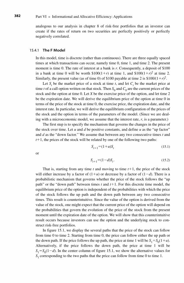
analogous to our analysis in chapter 8 of risk-free portfolios that an investor cancreate if the rates of return on two securities are perfectly positively or perfectlynegatively correlated.

15.4.1 The F Model

In this model, time is discrete (rather than continuous). There are three equally spacedtimes at which transactions can occur, namely time 0, time 1, and time 2. The presentmoment is time 0. The rate of interest at a bank is r. Consequently, a deposit of $100in a bank at time 0 will be worth $100(1�r) at time 1, and $100(1�r)2 at time 2.Similarly, the present value (as of time 0) of $100 payable at time 2 is $100/(1�r)2.

Let St be the market price of a stock at time t, and let Ct be the market price attime t of a call option written on that stock. Then S0 and C0 are the current prices of thestock and the option at time 0. Let X be the exercise price of the option, and let time 2be the expiration date. We will derive the equilibrium price of the option at time 0 interms of the price of the stock at time 0, the exercise price, the expiration date, and theinterest rate. In particular, we will derive the equilibrium configuration of the prices ofthe stock and the option in terms of the parameters of the model. (Since we are deal-ing with a microeconomic model, we assume that the interest rate, r, is a parameter.)

The first step is to specify the mechanism that governs the changes in the price ofthe stock over time. Let u and d be positive constants, and define u as the “up factor”and d as the “down factor.” We assume that between any two consecutive times t andt�1, the prices of the stock will be related by one of the following two paths:

St�1�(1�u)St (15.1)

or

St�1�(1�d)St . (15.2)

That is, starting from any time t and moving to time t�1, the price of the stockwill either increase by a factor of (1�u) or decrease by a factor of (1�d). There is aprobabilistic mechanism that governs whether the price of the stock follows the “uppath” or the “down path” between times t and t�1. For this discrete time model, theequilibrium price of the option is independent of the probabilities with which the priceof the stock follows the up path and the down path between any two consecutivetimes. This result is counterintuitive. Since the value of the option is derived from thevalue of the stock, one might expect that the current price of the option will depend onthe probabilities that govern the evolution of the price of the stock from the presentmoment until the expiration date of the option. We will show that this counterintuitiveresult occurs because investors can use the option and the underlying stock to con-struct risk-free portfolios.

In figure 15.1, we display the several paths that the price of the stock can followfrom time 0 to time 2. Starting from time 0, the price can follow either the up path orthe down path. If the price follows the up path, the price at time 1 will be S1�S0(1�u).Alternatively, if the price follows the down path, the price at time 1 will beS1�S0(1�d). In the center column of figure 15.1, we show the alternative values forS1 corresponding to the two paths that the price can follow from time 0 to time 1.


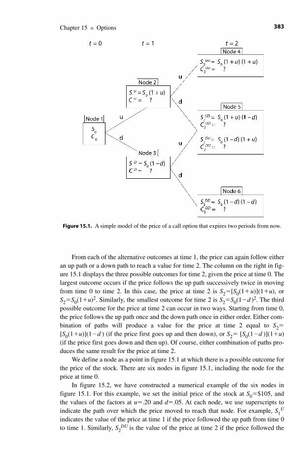
From each of the alternative outcomes at time 1, the price can again follow eitheran up path or a down path to reach a value for time 2. The column on the right in fig-ure 15.1 displays the three possible outcomes for time 2, given the price at time 0. Thelargest outcome occurs if the price follows the up path successively twice in movingfrom time 0 to time 2. In this case, the price at time 2 is S2�[S0(1�u)](1�u), orS2�S0(1�u)2. Similarly, the smallest outcome for time 2 is S2�S0(1�d )2. The thirdpossible outcome for the price at time 2 can occur in two ways. Starting from time 0,the price follows the up path once and the down path once in either order. Either com-bination of paths will produce a value for the price at time 2 equal to S2�

[S0(1�u)](1�d ) (if the price first goes up and then down), or S2� [S0(1�d )](1�u)(if the price first goes down and then up). Of course, either combination of paths pro-duces the same result for the price at time 2.

We define a node as a point in figure 15.1 at which there is a possible outcome forthe price of the stock. There are six nodes in figure 15.1, including the node for theprice at time 0.

In figure 15.2, we have constructed a numerical example of the six nodes in figure 15.1. For this example, we set the initial price of the stock at S0�$105, and the values of the factors at u�.20 and d�.05. At each node, we use superscripts toindicate the path over which the price moved to reach that node. For example, S1

U

indicates the value of the price at time 1 if the price followed the up path from time 0to time 1. Similarly, S2

DU is the value of the price at time 2 if the price followed the


Figure 15.1. A simple model of the price of a call option that expires two periods from now.

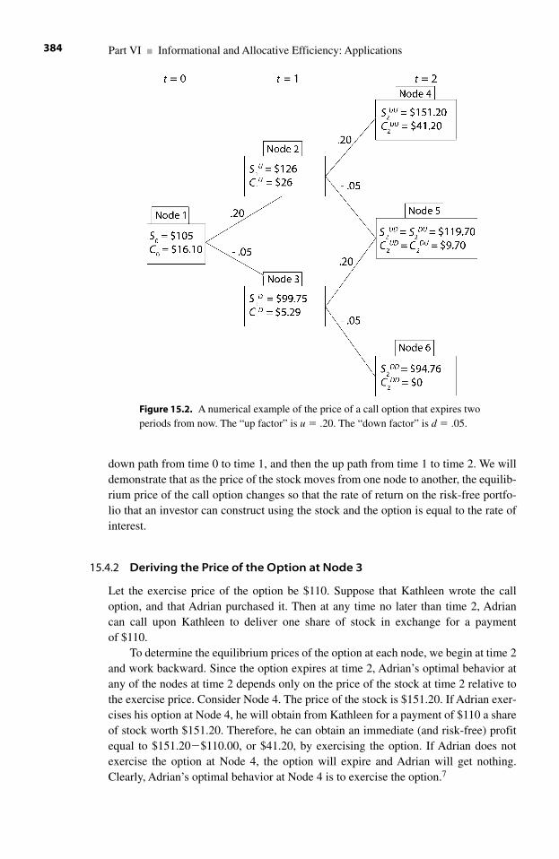
down path from time 0 to time 1, and then the up path from time 1 to time 2. We willdemonstrate that as the price of the stock moves from one node to another, the equilib-rium price of the call option changes so that the rate of return on the risk-free portfo-lio that an investor can construct using the stock and the option is equal to the rate ofinterest.

15.4.2 Deriving the Price of the Option at Node 3

Let the exercise price of the option be $110. Suppose that Kathleen wrote the calloption, and that Adrian purchased it. Then at any time no later than time 2, Adrian can call upon Kathleen to deliver one share of stock in exchange for a payment of $110.

To determine the equilibrium prices of the option at each node, we begin at time 2and work backward. Since the option expires at time 2, Adrian’s optimal behavior atany of the nodes at time 2 depends only on the price of the stock at time 2 relative tothe exercise price. Consider Node 4. The price of the stock is $151.20. If Adrian exer-cises his option at Node 4, he will obtain from Kathleen for a payment of $110 a shareof stock worth $151.20. Therefore, he can obtain an immediate (and risk-free) profitequal to $151.20�$110.00, or $41.20, by exercising the option. If Adrian does notexercise the option at Node 4, the option will expire and Adrian will get nothing.Clearly, Adrian’s optimal behavior at Node 4 is to exercise the option.7


Figure 15.2. A numerical example of the price of a call option that expires twoperiods from now. The “up factor” is u � .20. The “down factor” is d � .05.

There are two equivalent ways in which Adrian can obtain $41.20 at Node 4.First, he can exercise the option by paying $110 to Kathleen, receiving from her theshare of stock, and then immediately selling that share for $151.20. Second, Adriancan sell the option to another investor. At Node 4, any investor will pay $41.20 for theoption because she could recover that cost by immediately exercising the option.Competition among investors will prevent the price of the option from droppingbelow $41.20 at Node 4, and no investor will pay more than $41.20. Thus, the equilib-rium price of the option at Node 4 is $41.20.

Proceeding similarly, we conclude that the equilibrium price of the option atNode 5 is $119.70�$110.00, or $9.70.

At Node 6, the price of the stock is $94.76, which is less than the exercise price ofthe option. Consequently, at Node 6 the option is worthless. Were Adrian to exercisehis option at Node 6, he would pay Kathleen $110 to obtain a share of stock that isworth only $94.76. Clearly, Adrian will not exercise the option. Nor can he sell it.Since the option is about to expire, no investor will pay anything for the right topurchase for $110 a security whose current price is less than $110. Hence, the equilib-rium price of the option at Node 6 is zero.

We have now determined the prices of both the stock and the option in each of thethree nodes that can occur at time 2. These prices appear in the three boxes in the col-umn under t�2 in figure 15.2. We can now use that information to determine theprices of the option in Nodes 2 and 3. We will do so by forming a different risk-freeportfolio for each of Nodes 2 and 3. Consider Node 3 first.

Starting at Node 3, the prices of the stock and the option must travel either toNode 5 or to Node 6 during the next period. By knowing the prices of both the stockand the option in both Nodes 5 and 6, an investor can construct a portfolio that willgenerate a riskless rate of return during that period. That is, the investor’s rate ofreturn can be predicted with certainty at Node 3 even though he cannot predictwhether the prices of the stock and the option will travel to Node 5 or to Node 6.

At Node 3, let the investor construct a portfolio that contains one share of stockand h3 options. Since we know the price of the stock but not the price of the option atNode 3, the value of the investor’s portfolio at Node 3 will be (1)S1

D�(h3)C1D, or

(1)$99.75�(h3)C1D. That is, the investor must spend (1)$99.75�(h3)C1

D to constructthis portfolio. The investor’s rate of return on this portfolio from time 1 to time 2depends on whether the prices of the stock and the option travel to Node 5 or to Node 6. To create a riskless rate of return, the investor chooses the value of h3 so thatthe values of the portfolio in Node 5 and Node 6 are equal. Since we know the valuesof the prices of both the stock and the option in both nodes, this is easily done.

At Node 5, the value of the investor’s portfolio will be

(1)S2DU�(h3)C2

DU�(1)$119.70�(h3)$9.70. (15.3)

At Node 6, the value of the investor’s portfolio will be

(1)S2DD�(h3)C2

DD�(1)$94.76�(h3)$0. (15.4)

Let h3* be the value of h3 that equates the values of the portfolio in Nodes 5 and 6.

Then

h3*�($119.70�$94.76)/($0�$9.70)��2.57. (15.5)


Since h3* is negative, the investor constructs the risk-free portfolio at Node 3 by

selling (or selling short) 2.57 options for each 1 share of stock that he purchases.8 Thatis, his portfolio at Node 3 contains a long position in the stock and a short position inthe option written on that stock. Recall that a long position in an asset is a positionfrom which the investor will gain wealth if the price of the asset rises. If the investorholds a short position in an asset, he will gain wealth if the price of that asset falls.9

Let Robin create a risk-free portfolio at Node 3 by purchasing 1 share of stockand selling 2.57 call options. To sell these options, Robin uses an options broker tocreate the options, which the broker then sells to another investor, Don. Then Don hasthe right to purchase 2.57 shares of stock from Robin by paying her the exercise priceof $110 per share any time before the option expires at time 2.

Robin can use her short position in the option to finance a portion of her longposition in the stock. Since the price of the option at Node 3 is C1

D, Robin will receive2.57 C1

D by selling the options. Consequently, Robin’s net cost to construct her port-folio at Node 3 is

(1)$99.75�(2.57)C1D. (15.6)

To proceed, we need to define the liquidation value of a portfolio.The liquidation value of an investor’s portfolio is the amount of cash that she

could raise by selling each of the long positions in her portfolio, and by simultane-ously purchasing securities to offset each of the short positions. Consider the follow-ing example.

Maria constructed a portfolio one year ago by purchasing 100 units of Asset Xand selling short 50 units of Asset Y. Maria’s portfolio is long 100 units of X and short50 units of Y. To establish her short position, Maria borrowed 50 units of Y from a bro-ker and sold them for cash. Once she completed the construction of her portfolio,Maria owned 100 units of X and owed (to the broker) 50 units of Y. Maria’s short posi-tion in Y obligates her to return 50 units of that security to the broker. The fact that shesold the 50 borrowed units of Y for cash has no bearing on her obligation to the bro-ker. Typically, Maria would repay the broker by purchasing 50 units of Y in the openmarket and delivering them to the broker. When she does so, we say that she covers (or closes) her short position.

The liquidation value of Maria’s portfolio is equal to the market value of her longposition in X minus the market value of her short position in Y. Let the current price ofX be $16, and let the current price of Y be $20. To liquidate her portfolio, Maria wouldsell her 100 units of X at $16 per unit, gaining $1,600 in cash. To complete the liqui-dation, she must deliver 50 units of Y to the broker from whom she borrowed them.Since she does not hold any units of Y in her portfolio (which is the essence of beingshort in Y), she must purchase 50 units of Y in the open market. This purchase willcost her $20�50 units, or $1,000. Consequently, the liquidation value of her portfoliois $1,600�$1,000, or $600.

We return to the question of determining the equilibrium value of C1D, which is

the equilibrium price of the option at Node 3 in figure 15.2. Since Robin is at Node 3at time 1, at time 2 she will be either at Node 5 or at Node 6. If she reaches Node 5, shecan liquidate her portfolio by selling the share of stock that she owns and purchasing


2.57 options to offset her short position in that asset. Then the liquidation value of her portfolio at Node 5 will be (1)$119.70�(2.57) $9.70, or $94.77. Alternatively, if Robin reaches Node 6, the liquidation value of her portfolio will be worth(1)$94.76�(2.57)$0, or $94.76. At Node 6, the option is worthless, so Robin incurs nocost at Node 6 to cover her short position. Except for a rounding error, the values ofRobin’s portfolio are equal in Nodes 5 and 6. For definiteness, we use $94.76 as thecommon value of her portfolio at Nodes 5 and 6.

The portfolio that Robin constructs at time 1, at Node 3, is riskless because thereis no uncertainty about its value one period later at time 2. Consequently, in equilib-rium the rate of return on this portfolio must be equal to the rate of interest. We thenhave:

[(1)$99.75�(2.57)C1D](1�.10)�$94.76. (15.7)

The first term in square brackets in equation (15.7) is the amount of her ownmoney that Robin spends to construct the portfolio at Node 3. Solving equation (15.7)for C1

D produces the equilibrium price for the option at Node 3, namely:

C1D�$5.29. (15.8)

By comparing Node 3 and Node 6, we can see the distinction between the marketprice of the option and the value of the option if it were exercised immediately. Noticethat the price of the option at Node 3 is not equal to the price of the stock minus theexercise price of the option, or zero, whichever is greater. At Node 6, the price of the option is zero because the price of the stock is less than the exercise price of theoption, and the option is about to expire. No one would exercise the option at Node 6,and there are no future nodes for this option. At Node 3, the price of the stock is alsoless than the exercise price, so no one would exercise the option at Node 3 either. Butthe price of the option at Node 3 is greater than zero because there is a possibility thatat time 2 the prices of the stock and the option will be at Node 5, where the price of thestock exceeds the exercise price of the option. At both Nodes 3 and 6, the value ofexercising the option immediately is zero because the price of the stock at that node isless than the exercise price of the option. At Node 6, the market price of the option iszero because there is no possibility of reaching a further node. But at Node 3, the mar-ket price of the option is positive because the value of exercising the option couldbecome positive as the system moves beyond Node 3.


Proceeding as we did for Node 3, we first determine the structure of the riskless port-folio that Robin could form at Node 2. It is critical to recognize that the structure ofthis portfolio is different from the portfolio that she formed at Node 3. The reason isthat starting from Node 3, Robin will move either to Node 5 or to Node 6; Node 4 isunattainable from Node 3. But starting from Node 2, Robin will move either to Node4 or to Node 5; Node 6 is unattainable from Node 2.


To create a riskless portfolio at Node 2, let h2* be the number of options that

Robin should hold for each share of stock that she holds. The cost of her portfolio atNode 2 will be:

(1)$126.00�h2*C1

U. (15.9)

This portfolio will be riskless if its liquidation values in Nodes 4 and 5 are equal.Equating these liquidation values produces:

(15.10)

Solving (15.10) for h2* yields

(15.11)

Note that the structures of the riskless portfolios at Nodes 2 and 3 are different.The portfolio at Node 2 contains 1 option held short for each share of the stock heldlong. At Node 3, the portfolio contains 2.57 options held short for each share of stockheld long.

The common liquidation value of the riskless portfolio at Nodes 4 and 5 is:

(15.12)

Substituting h2*��1 into equation (15.9), the cost of the portfolio at Node 2 is

(1)$126.00�(1)C1U. Since the portfolio is riskless, the equilibrium rate of return is

.10, which requires:

(15.13)

which produces the equilibrium value for the price of the option at Node 2 as:

(15.14)

In Node 2, we again see the distinction between the exercise value and the marketvalue of the option. The exercise value of the option at Node 2 is the cash that aninvestor would receive by exercising the option when the price of the stock is $126.This exercise value is $126�$110, or $16. But the market value of the option at Node2 is $26, which reflects the possibility that the system could move to Node 4 fromNode 2. If an investor who owned an option at Node 2 wanted to liquidate that option,clearly he would sell it to another investor (for $26) rather than exercise it (whichwould yield only $126�$110, or $16).


We can now use the equilibrium values for the prices of the option at both Nodes 2 and3 to derive the equilibrium price of the option for time 0 (at Node 1). Let h1

* bethe number of options that Robin should hold for each share of stock to form a

C U1 $26.�

[(1)$126.00 (1) ](1 .10) $110,1� � �C U

(1)$151.20 (1)$41.20 (1)$119.70 (1)$9.70.

$110.00.

� � �

�

h2* 1.��

(1) (1) , or

(1)$151.20 $41.20 (1)

2 2*

2 2 2*

2

2*

S h C S h C

h

UU UU UD UD� � �

� � $$119.70 $9.70.2*�h


riskless portfolio at Node 1. Then h1* is the solution to

(15.15)

which yields:

(15.16)

The common value of the riskless portfolio at Nodes 2 and 3 will be:

(15.17)

or $93.00 (approximately).The cost of the portfolio at Node 1 is:

(15.18)

Then equilibrium requires that:

(15.19)

so that the equilibrium price of the option at Node 1 (at time 0) is $16.11.

15.4.5 Extending the Binomial Model to N Periods

In the preceding sections, we analyzed a binomial model for the case in which thereare two periods remaining until the option expires. It should be obvious that we couldextend the analysis to the case in which N periods remain until the option expires. Thelarger the value of N, the larger the number of nodes. But so long as N is a finite inte-ger, we can determine the prices of the stock and the option for each of the terminalnodes. Then for each node at which the system can be located when there is only oneperiod remaining until expiration, there will be only two nodes to which the systemcan travel during the final period. We can then construct a riskless portfolio to obtainthe equilibrium price of the option at each of the nodes that is one period away fromthe expiration date of the option. Proceeding backward through time, we can deter-mine the equilibrium price of the option at time 0.10

By fixing the date of expiration and letting the number of periods increase with-out limit, we could obtain the formula for the equilibrium price of an option for thecase in which the rate of return on the underlying stock is continuously compounded,rather than periodically compounded, as is the case in a binomial model. Instead ofpursuing this further, we shall move immediately to the Black-Scholes formula, fol-lowing a summary of the properties of the binomial model.

15.4.6 Summary of the Simple Model of the Price of a Call Option

The simple model that we have presented in this section is sufficient to illuminate theessential properties of the Black-Scholes option pricing formula that we discuss in thefollowing section. To prepare for that discussion, we summarize briefly the features of

[(1)$105.00 (1.27) ](1 .10) $93.00,0� � �C

(1)$105.00 (1.27) .0� C

(1)$126.00 (1.27)$26.0 (1)$99.75 (1.27)$5.29,� � �

h1* 1.27.� �

(1) (1) , or

(1)$126.00 $26.0 (1)$99.7

2 1*

2 2 1*

2

1*

S h C S h C

h

U U D D� � �

� � 55 $5.29,1*�h


the simple model. These features reflect the application to the pricing of options of thefundamental principles that we have used throughout the book.

First, equilibrium is a configuration of prices and quantities with the property thatno economic agent has an incentive to change his or her decisions. In particular, if theprice of a stock and the price of a call option written on that stock are in equilibrium,no investor will have an incentive to change the allocation of funds between the stockand the option.

Second, if an investor can construct a riskless portfolio by combining two or moreassets in certain proportions, then the rate of return on that portfolio must be equal tothe rate of interest available at a bank. The rate of return on a portfolio depends on therates of return of its constituent assets and on the proportions in which the investorallocates funds among those assets. Further, the rate of return on an asset depends onthe current prices of those assets. Consequently, requiring the rate of return on theportfolio to be equal to the interest rate imposes a condition on the relationship amongthe prices of the assets in the portfolio.

Third, the equilibrium price of the option has several properties that are apparentfrom the model presented above.

1. The most counterintuitive property is that the equilibrium between the price ofa call option and the price of the underlying stock does not depend on the expectedrate of return of the underlying stock. The price of the call does depend on the currentprice of the stock and on the variance of the rate of return on the stock. It is critical torecognize here that the model determines the equilibrium price of the call, conditionalon the price of the underlying stock. The model does not predict the price of the callindependently of the price of the stock. Finally, the model determines only the relativeprices of the option and the underlying stock, not the absolute values of these prices.

In the simple model presented in this section, the magnitudes of the up and downfactors are a proxy for the variance of the rate of return on the stock. If the up factorwere to increase, the maximal possible value for the price of the stock at time 2 wouldincrease. Similarly, if the down factor were to increase (so that the price of the stockcould fall more rapidly on any of the down branches), the minimal value for the priceof the stock at time 2 would decrease. The consequent increase in the range of possi-ble values for the price of the stock at time 2 will increase the variance of the rate ofreturn on the stock.11

An increase in the variance of the stock’s rate of return increases the likelihoodthat on the expiration date of the option, the price of the stock will be significantlyabove, or significantly below, the exercise price of the option. The market value of thecall option on its expiration date depends asymmetrically on the price of the stock onthat date. The amount by which the price of the stock falls below the exercise price of the option on the expiration date is irrelevant; once the price of the stock falls belowthe exercise price of the option, the market value of the option is zero.12 The converseis not true. On the expiration date, each $1 increase in the price of the stock above theexercise price of the option increases the market value of the option by $1.Consequently, an increase in the variance of the rate of return on the stock increasesthe current market value of the call. Increases in both the up factor and the down fac-tor will increase the variance of the rate of return on the stock, and thus increase thecurrent market value of the call option.


2. The longer the time until the option expires, the more opportunity there is forthe price of the stock to move above the exercise price of the option before the optionexpires. Therefore, the more distant the expiration date, the higher the current price ofthe option.

3. As implied by the arguments above, the greater the amount by which the exer-cise price of the option exceeds the current price of the stock, the lower the currentprice of the option.

We used the model presented in this section to determine the equilibrium relation-ship between the prices of the call option and the underlying stock. There is an analo-gous model for a put option. Since the arguments in the two models are symmetric, wedo not develop the model for put options. In our model for a call option, we used anextremely simple mechanism to govern the evolution of the price of the stock overtime. In the next section, we describe the more realistic model produced by Black andScholes to determine the equilibrium prices of options.

15.5 The Black-Scholes Option Pricing Formula

The model in the preceding section illustrates the economic rationale for the equilib-rium price of an option. But that model is too simple to produce an empirically reli-able formula. In this section we present, but do not derive, the Black-Scholes optionpricing formula. This formula is widely used by both economists and investors. Priorto the appearance of this formula, the volume of organized trading in options was asmall fraction of what it is today. By providing an intuitively rational and empiricallyverified procedure for determining the equilibrium price of an option, the formulareduced the risk of trading in options.

This does not mean that trading in options is not risky. Predicting the price of anysecurity requires two steps. First, one must understand how specific kinds of informa-tion will affect the equilibrium price of the security. Second, one must predict howthose pieces of information will change over time. For example, the Black-Scholesformula states the relationship between the equilibrium price of the option and thevariance of the distribution of future prices for the underlying stock. The Black-Scholes formula does not, however, predict how that variance might change over time.Hence we have the distinction, first mentioned in section 9.5.2 of chapter 9, betweenpredicting the equilibrium price that corresponds to a specific set of information andpredicting that information itself.

15.5.1 The Differences between the Simple Model and the Black-Scholes Formula

In the simple model of the preceding section, transactions could occur only at equallyspaced times. Treating time as discrete, rather than as continuous, facilitates analysisbut sacrifices accuracy. Competition among investors adjusts security prices to newinformation, and information arrives irregularly through time. Moreover, in an effi-cient market the adjustment to new information is immediate.13 A model that restricts


transactions to discrete times is unlikely to produce accurate predictions, even thoughthat model might produce valuable hints of how options would be priced in actual (as opposed to hypothetical) markets.

The Black-Scholes model is analogous to, but much more sophisticated than, themodel in the preceding section. In particular, in the Black-Scholes model time is acontinuous variable. The models are analogous in that they both recognize that aninvestor can use the option and the underlying stock to construct a risk-free portfolio.Then the equilibrium relationship between the prices of the option and the stock fol-lows from the condition that the rate of return on the portfolio must be equal to the rateof return on the risk-free asset.

Whether time is discrete or continuous, the number of options that the investormust hold for each share of stock to construct a risk-free portfolio depends on the cur-rent prices of both securities and on the time remaining until the option expires.Consequently, if time is discrete, the investor must adjust the portfolio periodicallyover time. But if time is continuous, the investor must adjust the portfolio continu-ously over time. A rigorous derivation of the Black-Scholes option pricing formula isbeyond the scope of this book. We instead present the formula and discuss its mainproperties.

15.5.2 The Black-Scholes Formula for the Price of a Call Option

In the Black-Scholes model, time is continuous. Investors can trade at any momentrather than being limited to trading periodically. Because time is continuous, we rep-resent the rate of return on a stock as a continuously compounded random variable.The relationship between periodic and continuous compounding is easily explained,which we do in the appendix to this chapter.


C0� The current market price of a call option written on IBM stock.

E� The exercise price of the call option.

S0� The current market price of a share of IBM stock.

T� The number of years remaining until the option expires (since time is acontinuous variable, T need not be an integer).

r� The continuously compounded annual rate of return on the risk-freeasset.

� The standard deviation of the continuously compounded annual rate ofreturn on a share of IBM stock.

ln(S0/E)� The natural logarithm of (S0/E).

N(d)� The probability that a normally distributed random variable will take avalue less than or equal to d. That is, N(d) is the area under the normalprobability density function to the left of the point d on the horizontalaxis, expressed as a proportion of the total area under the density function.


The Black-Scholes option pricing formula is:

in which

(15.20)

Although the problem of deriving the formula in equation (15.20) was intellectu-ally formidable, the application of the formula is less formidable than it might appear.With the exception of the standard deviation, , all the terms on the right side of(15.20) are readily available. The financial exchanges post the current price of thestock, the rate of return on the risk-free asset, and the exercise price and the expirationdate of the option. Once we have an estimate of , we can calculate the values of d1and d2 from a table of probabilities for a normally distributed random variable. We canestimate the value of from historical data on the rate of return of the stock.Consequently, we can use equation (15.20) to obtain the equilibrium price of the calloption, conditional on our estimate of . One indication of the value of the Black-Scholes formula in the investment community is that there are handheld calculatorsthat include a program to evaluate the Black-Scholes formula. All the investor need dois enter the values for the variables and the parameters on the right side of equation(15.20), press a button, and obtain the corresponding value for the equilibrium price ofthe call option.

Using historical data on the rate of return on the stock to estimate the value of is problematic. Any formula for the equilibrium price of a security is based on infor-mation about the future rates of return for that security. The Black-Scholes formula isno exception. This formula establishes the equilibrium price of the call based on thestandard deviation of the future rates of return on the stock. The probability distribu-tion for future rates of return on the stock need not be identical to the distribution thatgenerated the rates of return observed in the past.

There is an interesting twist to the problem of estimating the standard deviation.We can use the Black-Scholes formula to estimate the value of for the future rates ofreturn on the stock, conditional on the current market prices of the call and the under-lying stock and the current values of the other parameters. Since a financial security isa claim on a sequence of future payments, the current market price of the securitydepends on the future values of the parameters that will govern those future payments.If we have confidence in the Black-Scholes formula, it is reasonable to expect thatspeculators will keep the current market prices of the call and the underlying stockequal (or close) to the values specified by the Black-Scholes formula in equation(15.20), given the values of the parameters that will affect the future rates of return onthe stock. Consequently, we can use the Black-Scholes formula to estimate the valueof σ for the future rates of return on the stock that are implied by the current marketprices of the option and the stock, and the values of the other parameters.

dS E r T

T

dS E r T

T

10

2

20

2

ln( / ) ( /2)

ln( / ) ( /2)

��

��

C S N d N d E erT0 0 1 2( ) ( )( / ),� �


The sensitivity of the formula in equation (15.20) to the estimate of is under-standable. Our analysis of the simple model in the preceding section showed that thecurrent price of the call option depends significantly on the range of values that theprice of the stock can reach on the date that the option expires. In the Black-Scholesformula, the larger the standard deviation of the rate of return on the stock, the widerthe range of terminal values for the price of the stock.

15.6 The Put-Call Parity

In this section, we present and explain the relationship that will hold in equilibriumamong the price of a stock and the prices of put and call options written on that stock.We know that an equilibrium in a financial market is a configuration of prices (andquantities) of securities with the property that no investor has an incentive to reallo-cate wealth among securities. In some cases, we can define the equilibrium as theabsence of any opportunities for an investor to obtain a risk-free profit. The put-callparity is one of these cases.


S0 and S1�the prices at time 0 and time 1 of a stock

C0 and C1�the prices at time 0 and time 1 of a call option written on that stock

P0 and P1�the prices at time 0 and time 1 of a put option written on that stock

E�the exercise price for both options

rf �the risk-free rate of interest

Assume that the stock pays no dividends between time 0 and time 1, and that bothoptions expire at time 1.

The put-call parity states that in equilibrium, the prices of the stock and the twooptions must satisfy:

S0�C0�E/(1�rf )�P0. (15.21)

We can develop the economic intuition of the put-call parity by regarding eachside of equation (15.21) as the cost of a different portfolio at time 0, and then showing that the values of both portfolios will be equal to S1 at time 1. If two differentportfolios that an investor could construct at time 0 produce the same value at time 1,then equilibrium requires that the two portfolios have the same value at time 0.

The left side of equation (15.21) is the cost at time 0 of a portfolio that contains a long position in one share of the stock. At time 1, the value of this portfolio will be S1.

The right side of equation (15.21) is the cost at time 0 of a portfolio that containslong positions in two assets and a short position in a third asset. The two assets heldlong are one unit of the call option and a bank account worth E/(1�rf); the asset heldshort is one unit of the put option. An investor, Michael, could construct this portfolioat time 0 by purchasing one call option, depositing E/(1�rf) in a bank, and selling(that is, writing) one put option. The sum of the first two terms on the right of equation


(15.21) is the value at time 0 of the long side of the portfolio. Michael would financepart of the cost of the long side of his portfolio by selling one put option.Consequently, the right side of equation (15.21) is the net cost to Michael at time 0 ofconstructing a portfolio that contains a long position in one call, a long position in abank account worth E/(1�rf), and a short position in one put.

At time 1, the price of the stock will be greater than, less than, or equal to theexercise price of the options. We will now show that in each case the amount of cashthat Michael could raise at time 1 by liquidating his portfolio will be S1. Recall that toliquidate a portfolio is to sell the assets held long and purchase assets to offset thepositions held short.

Suppose that S1� E. Consider first the long side of the portfolio. Since the calloption expires at time 1, its market value will be equal to S1�E. That is, Michaelcould sell his call option for S1�E in cash. Any investor will pay S1�E for the right topurchase for E a security that can be immediately resold for S1. The second asset thatMichael holds long is his bank account. This account will have grown from E/(1�rf)at time 0 to [E/(1�rf)](1�rf)�E at time 1. Then at time 1, Michael can liquidate thelong side of his portfolio for S1�E�E, or S1, in cash.

Alternatively, at time 1 Michael can exercise the call option to obtain a share ofstock, using the funds in the bank account to pay the exercise price, E. He can then sellthe stock, thereby raising S1 in cash.

The short side of Michael’s portfolio contains one put option. To hold a shortposition in an asset is to have an obligation to deliver that asset or its equivalent. IfMichael’s short position contained one share of stock, he would have to deliver oneshare of stock, or its equivalent, to liquidate that position. Consequently, the cost toMichael of liquidating at time 1 a short position in one share of stock would cost himS1. (If Michael delivers the share from his own inventory, he incurs an implicit cost ofS1. If he purchases at time 1 the share that he delivers, he incurs an explicit cost of S1.)

But Michael’s short position is in the put option, not in the stock. The investorwho purchased the put from Michael at time 0 has a right to require Michael to pur-chase one share of stock and pay the exercise price, E. But at time 1 Michael knowsthat the investor will allow her put option to expire unexercised because S1 �E. Toexercise the put at time 1 would be to sell to Michael for E a share of stock that isworth more than E. Consequently, the put is worthless at time 1, and thus Michael willincur no cost to liquidate the short side of his portfolio.

We conclude that if S1�E, the value of Michael’s portfolio at time 1 will be S1.Suppose that S1E. In this case, the call option that Michael holds long is worth-

less at time 1. No investor at time 1 will pay anything for the right to acquire for E ashare of stock that is worth less than E. Hence, Michael will allow his call option toexpire unexercised. His bank account at time 1 is again worth E. Then the long side ofhis portfolio at time 1 is worth 0�E�E.

On the other side of his portfolio, Michael has a short position in one put option.The investor who purchased the put option from Michael at time 0 will exercise thatoption against him at time 1. By doing so, the investor will sell to Michael for E ashare of stock that is worth, at time 1, less than E. Since Michael’s bank account isworth E at time 1, Michael can use those funds to discharge his obligation under theput option. We conclude that after he covers his short position in the put option at


time 1, Michael will own one share of stock that is worth S1. Consequently, the valueof his portfolio at time 1 is S1.

Suppose that S1�E. In this event, both the call option and the put option areworthless. No one would bother to exercise a right to buy or sell, for E, one share ofstock that is worth E. Michael’s bank account is worth E at time 1. But in this case,E�S1. Then the value of Michael’s portfolio at time 1 is S1.

We have established that for all three possible outcomes for time 1, the value attime 1 of the portfolio represented by the right side of equation (15.21) is S1.Obviously, the value at time 1 of the portfolio represented by the left side of (15.21) isalso S1. Since the values of the two portfolios at time 1 are equal, their values at time0 must also be equal, which establishes the put-call parity stated in (15.21).

15.6.1 Arbitrage and the Put-Call Parity

The put-call parity specifies a relationship among the equilibrium values of the pricesof the put, the call, and the underlying stock. We can appreciate this relationship byconsidering how an investor could obtain a riskless profit whenever the prices of thestock and the two options do not satisfy equation (15.21).

Suppose that the stock is overpriced relative to the options. Then:

S0�C0�E/(1�rf )�P0. (15.22)

If equation (15.22) holds, then we may write:

S0�P0�C0�E / (1�rf ) (15.23)

Equation (15.22) states that a portfolio that contains the stock and the put optionis overpriced relative to a portfolio that contains the call option and the bank accountworth the present value of the exercise price. Under these circumstances, an investorcould obtain a riskless profit by simultaneously selling the portfolio on the left side ofequation (15.23) and purchasing the portfolio on the right.

The amount of risk-free profit will be equal to the value of the left side of (15.23)minus the value of the right side. We will now demonstrate this result.

At time 0, let Michael construct a single portfolio as follows:

1. Sell short one share of stock, obtaining revenue equal to S0.2. Sell one put option, obtaining revenue equal to P0.3. Buy one call option, incurring a cost equal to C0.4. Deposit E/(1�rf) in a bank account. [That is, purchase a bank account that has

a balance equal to E/(1�rf).]

Using equation (15.23), the amount of cash that Michael will obtain at time 0 byconstructing this portfolio is:

S0�P0�C0�E / (1�rf )�0. (15.24)

We will now show that at time 1 the net value of Michael’s portfolio will be zerowith certainty. That is, the cash that he can raise by liquidating his two long positionswill be equal to the cash that he will need to cover his two short positions.


Consequently, the positive net revenue in equation (15.24) is a risk-free profit forMichael at time 0.

Suppose that S1�E. On the long side of his portfolio, Michael owns a call optionand a bank account. The call is “in the money”; by exercising the call, Michael canpurchase for E a share of stock that is worth S1�E. The value of his bank account attime 1 is E. Then Michael can obtain a share of stock by exercising his call option,using the balance in his bank account to pay the exercise price. Consequently, Michaelcan convert the long side of his portfolio from containing one call and one bankaccount to containing one share of stock that is worth S1. Alternatively, Michael cansell his call option for S1�E in cash, and liquidate his bank account for E in cash. Hisnet cash will then be S1�E�E�S1.

On the other side of his portfolio, Michael is short one put option and one share ofstock. Since S1�E, the put is worthless. The investor who purchased the put fromMichael at time 0 will not exercise it at time 1; to do so would be to deliver to Michaela share of stock worth S1 and accept ES1 in exchange. Then Michael’s only obliga-tion is to cover his short position in the stock. He can do this by delivering to the bro-ker from whom he borrowed a share at time 0 the share of stock that he obtains at time1 by exercising his call option. Or if Michael sells his call option for S1�E and liqui-dates his bank account for E, he can deliver S1 in cash to the broker, who could thenpurchase the share of stock himself. Then Michael’s net revenue (and net cost) at time1 is zero. Consequently, the net revenue in equation (15.24) that Michael obtained attime 0 is a clear profit; he never pays for it.

Suppose that S1E. In this event, the put option is in the money at time 1 and thecall option is worthless. The investor who purchased the put option from Michael attime 0 will exercise it against him at time 1 by delivering to Michael one share ofstock (which is worth less than E) and collecting from Michael the exercise price, E.Michael can pay the exercise price by liquidating his bank account, which will beworth E at time 1. Michael can now use the share of stock that he obtains when the putis exercised against him to cover his short position in the stock by delivering the shareof stock to the broker from whom he borrowed it at time 0. Michael’s net gain at time1 is zero, and therefore the revenue in equation (15.24) that he obtained attime 0 is a clear profit.

Suppose that S1�E. In this event, both the put option and the call option areworthless at time 1. As in all cases, his bank account is worth E at time 1. Michael canthen liquidate his bank account, use the proceeds to purchase one share of stock at acost of S1�E, and deliver that share to the broker from whom he borrowed it at time0. Again, Michael’s net gain at time 1 is zero; the positive net revenue in equation(15.24) that he obtained at time 0 is a clear profit.

15.7 Homemade Options

In several places in this book, we have provided examples of “homemade” items thatindividual investors can use to expand their opportunities for mutually beneficialexchanges and thus increase the efficiency of the allocation of their resources. Thefirst example was a homemade dividend, presented in chapter 5. In the chapters on


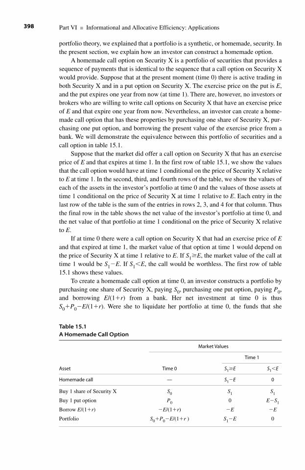
portfolio theory, we explained that a portfolio is a synthetic, or homemade, security. Inthe present section, we explain how an investor can construct a homemade option.

A homemade call option on Security X is a portfolio of securities that provides asequence of payments that is identical to the sequence that a call option on Security Xwould provide. Suppose that at the present moment (time 0) there is active trading inboth Security X and in a put option on Security X. The exercise price on the put is E,and the put expires one year from now (at time 1). There are, however, no investors orbrokers who are willing to write call options on Security X that have an exercise priceof E and that expire one year from now. Nevertheless, an investor can create a home-made call option that has these properties by purchasing one share of Security X, pur-chasing one put option, and borrowing the present value of the exercise price from abank. We will demonstrate the equivalence between this portfolio of securities and acall option in table 15.1.

Suppose that the market did offer a call option on Security X that has an exerciseprice of E and that expires at time 1. In the first row of table 15.1, we show the valuesthat the call option would have at time 1 conditional on the price of Security X relativeto E at time 1. In the second, third, and fourth rows of the table, we show the values ofeach of the assets in the investor’s portfolio at time 0 and the values of those assets attime 1 conditional on the price of Security X at time 1 relative to E. Each entry in thelast row of the table is the sum of the entries in rows 2, 3, and 4 for that column. Thusthe final row in the table shows the net value of the investor’s portfolio at time 0, andthe net value of that portfolio at time 1 conditional on the price of Security X relativeto E.

If at time 0 there were a call option on Security X that had an exercise price of Eand that expired at time 1, the market value of that option at time 1 would depend onthe price of Security X at time 1 relative to E. If S1�E, the market value of the call attime 1 would be S1�E. If S1E, the call would be worthless. The first row of table15.1 shows these values.

To create a homemade call option at time 0, an investor constructs a portfolio bypurchasing one share of Security X, paying S0, purchasing one put option, paying P0,and borrowing E/(1�r) from a bank. Her net investment at time 0 is thusS0�P0�E/(1�r). Were she to liquidate her portfolio at time 0, the funds that she


Table 15.1A Homemade Call Option

Market Values

Time 1

Asset Time 0 S1�E S1E

Homemade call — S1�E 0

Buy 1 share of Security X S0 S1 S1

Buy 1 put option P0 0 E�S1

Borrow E/(1�r) �E/(1�r) �E �E

Portfolio S0�P0�E/(1�r ) S1�E 0

would gain by selling her one share of Security X and her put option would be justsufficient to pay off her loan.

At time 1, the value of the investor’s portfolio will be equal to the revenue thatshe could obtain by selling the two assets in her long position, minus the expenditurethat would be required to repay her loan. Selling the one share of Security X and theone put option will generate revenue equal to S1�P1. To repay her loan will cost E.Therefore, the net value of her portfolio at time 1 will be S1�P1�E.

The market price of the put option at time 1 depends on the value of S1 relative toE. If S1�E, the put option is worthless. If S1E, the put option will be worth E�S1.We conclude that if S1�E, the value of the investor’s portfolio at time 1 will beS1�P1�E�S1�0�E�S1�E. If S1E, the portfolio at time 1 will be worthS1�P1�E�S1�(E�S1)�E�0. Thus, for any given value of Security X at time 1, thevalue of the homemade call option that expires at time 1 and that has an exercise priceof E will be equal to the value of a conventional call option with those properties.

The value at time 0 of the homemade call option is S0�P0�E/(1�r). Since thehomemade call option is economically equivalent to a conventional call option, theprice at time 0 of a conventional call option must also be equal to S0�P0�E/(1�r).The alert reader will see that this assertion is equivalent to the put-call parity in equa-tion (15.21).

15.8 Introduction to Implicit Options

The groundbreaking contribution that Fischer Black and Myron Scholes made to theeconomics of finance, and to the practice of finance, by producing their option pricingformula is well known. Less well known is their insight that some configurations offinancial securities and capital structures of firms contain implicit options. An implicitoption is an opportunity that is sufficiently like a conventional option that we can use the option pricing formula to infer some information about that opportunity thatwill enable investors to effect mutually beneficial exchanges that would otherwise beforegone.

Economic efficiency requires that firms and investors undertake all mutually ben-eficial exchanges. Some potentially beneficial exchanges are foregone because thecosts of acquiring reliable information about future outcomes are too high. In situa-tions that contain implicit options, we can use the theory of option pricing to increaseallocative efficiency by reducing the costs of acquiring information.

We examine two uses of implicit options. First, we use the concept to determinethe equilibrium allocation of a leveraged firm’s total market value between its commonstock and its bonds. Specifically, we explain how the common stock-holders of the firmhold an implicit option to purchase the firm from the bondholders. We can then use theoption pricing formula to infer properties of the prices of both securities.

Second, we explain how a firm’s decision on whether to invest in a new projectcan involve an implicit call option. Owning a call option on a security enables aninvestor to postpone the decision on whether to purchase that security while preserv-ing the right to obtain the security at the fixed exercise price specified by the option.


The investor can use the time until the option expires to collect information that couldreduce uncertainty about the future rates of return on the security. The market price ofthe call option is the investor’s opportunity cost of continuing to hold the option,rather than selling it or exercising it.14 Therefore, the market price of the option is theinvestor’s implicit marginal value of information about the security (net of the explicitcosts of collecting the information).

Under some conditions, the investor’s situation just described is analogous to thatof a firm that can postpone a decision to invest in a new project whose initial costs areirrecoverable (sunk) and whose future earnings are uncertain. A benefit of investing inthe project without delay is that the firm will receive the revenues from the projectsooner than if the firm postponed the project. A cost of investing in the project withoutdelay is the value of the foregone opportunity to collect information that could leadthe firm to reject the project and thus avoid losing the initial sunk costs. The value ofthe option to collect information by postponing the decision on the project is one ofthe opportunity costs incurred if the firm begins the project now. To maximize itsshareholders’ wealth, the firm should include this opportunity cost when decidingwhether to begin the project now or postpone a decision on the project in order toacquire more information. A familiarity with options is useful for recognizing theexistence of these implicit options and in calculating their values.

Consequently, recognizing implicit options and using option pricing theory todetermine their values can increase economic efficiency by increasing the accuracy ofthe net present values of investment projects.

15.9 Implicit Options in a Leveraged Firm

In chapter 13, we explained that the capital structure of a firm can affect the extent towhich investors can effect mutually beneficial exchanges. A simple but typical formof capital structure consists of common stock and bonds. The former are residualclaims on the firm’s earnings; the latter are contractual claims. In chapter 13, weprovided several examples of how investors could expand their opportunities formutually beneficial exchanges by including both residual claims and contractualclaims in the capital structure of their firms.

We will now use option pricing theory to determine the equilibrium allocation of the total value of a firm between the investors who own the common stock and theinvestors who own the bonds. By definition, the sum of the market values of the stock and the bonds is the market value of the firm. That is, if an investor were topurchase all the shares of the common stock and all the bonds, that investor wouldhold a claim to all of the firm’s earnings. But this fact does not tell us how the finan-cial markets will allocate the total value of the firm between the shareholders and thebondholders.

We begin by recalling the distinction that we offered in section 13.2 of chapter 13between the legal significance and the economic significance of the differencebetween shareholders and bondholders. By law, the shareholders own the firm; thebondholders are creditors of the firm. As owners, the shareholders elect a board of


directors, who then hire professional managers to operate the firm. Ultimately, theshareholders control the firm’s operations, including its choice of projects in which toinvest.15 As residual claimants, the shareholders own whatever remains of the firm’searnings after the firm discharges its contractual obligations. As residual claimants,the shareholders have no right to bring legal action against the firm, its managers, orits directors if the residual earnings fall below some threshold. If there is little or nothing left for the shareholders after the contractual claimants are paid, so be it.

As creditors, the bondholders hold a contract with the firm. In consequence, thebondholders do have a right to bring legal action if the firm fails to make the paymentsspecified in the contract. The bondholders do not, however, own anything other thanthis contract.

A legal analysis of common stocks and bonds addresses the nature of the rightsthat pertain to the two kinds of securities. Accordingly, a legal analysis would deter-mine how the rights held by the owners of each security are affected by various out-comes. For example, who has the right to determine whether the firm should invest ina project that would substantially increase the risk that the firm might fail to make therequired payments to the bondholders on time? In contrast to a legal analysis, an eco-nomic analysis of common stocks and bonds is concerned with the market prices ofthe securities. The market price of a security depends ultimately on investors’ percep-tions of the probability density functions that govern the future payments generated bythose securities, rather than on the legal definitions of the rights attached to thosesecurities.

We will now construct a simple model of a firm to demonstrate how the existenceof bonds in the firm’s capital structure creates an implicit option. We then use optionpricing theory to determine the equilibrium allocation of the total value of the firmbetween the bondholders and the shareholders.

15.9.1 An Implicit Option for the Shareholders Written by the Bondholdersof the Mosquito Point Barge Company

The Mosquito Point Barge Company carries fertilizer and other agricultural inputsalong the Seneca River. The company owns several barges and tugboats, financingthese assets by issuing a sequence of one-year bonds. Specifically, at the beginning ofeach year the company sells 10,000 new bonds at a market price of $850 each. Eachbond has a face value of $1,000 and matures one year after the company issues it.Consequently, the firm has a contractual obligation to pay the bondholders a total of$10,000,000 ($1,000 times 10,000 bonds) at the end of each year to redeem the bondsthat were issued at the beginning of that year. The bonds are zero-coupon bonds.Accordingly, the firm makes no explicit payments of interest on the bonds. Aninvestor’s return from holding one of the bonds arises from the difference between themarket price of the bonds and their face value. In the present example, the investor’srate of return would be ($1,000�$850)/$850, or $150/$850, or .177 (approximately).

By selling 10,000 new bonds at the beginning of each year at a price of $850 perbond, the Mosquito Point Barge Company finances $8,500,000 worth of equipment.By redeeming the bonds at the end of each year for a total of $10,000,000, the com-pany pays a finance charge equal to $1,500,000 per year. Since the company repeats


this process each year, the company is perpetually in debt. Before concluding that thisis a bad arrangement, remember that the company’s alternative to using bondholdersto finance the equipment would be to have the shareholders finance it. If the share-holders financed the equipment by permanently contributing an additional $8,500,000in capital, they would perpetually incur an opportunity cost on this capital. Thus, aswe have learned, the shareholders must either pay interest explicitly, by having theirfirm issue a perpetual sequence of one-year bonds, or they must pay interest implicitlyby contributing an additional $8,500,000 in capital that they could have invested elsewhere.

We turn now to the implicit option created for the company’s shareholders by theexistence of these bonds. At the end of each year, the shareholders must decidewhether to continue operating their firm for at least one more year or to liquidate thefirm. To operate for one more year, the shareholders must redeem the maturing bonds.The maturity (face) value of these bonds is $10,000,000. The shareholders can raisepart of this $10,000,000 by issuing a new set of one-year bonds. If the new bonds havezero coupons and an aggregate face value of $10,000,000, as do the bonds that arenow maturing, the shareholders will have to sell the new bonds at a discount fromtheir face value. Consequently, the shareholders will have to use part of the revenuetheir firm earned during the year now ending to make up the difference between thereceipts from the sale of the new bonds and the $10,000,000 they need to redeem thematuring bonds.

Alternatively, if the shareholders decide to liquidate the firm, they could simplyabandon the firm to the owners of the bonds that are now due for redemption. That is,the shareholders could allow the bonds to go into default, in which case the bondhold-ers would acquire the right to take over the firm and either operate it themselves or sellthe equipment in an attempt to recover the $10,000,000 owed to them by the share-holders.

In effect, the shareholders have an implicit call option to purchase the firm fromthe bondholders at the end of each year by paying an exercise price of $10,000,000. Ifthe shareholders expect that the firm’s future earnings will be sufficiently high, theshareholders will exercise their option to retain control of the firm by redeeming thematuring bonds. Otherwise, the shareholders will let their implicit option to retaincontrol of the firm expire by not redeeming the maturing bonds.

The shareholders have a sequence of implicit options. Each option expires at theend of a year. To exercise an option is to retain control of the firm for one more year.The exercise price of each option is the aggregate face value of the bonds that are nowmaturing. To operate the firm for a sequence of years, the shareholders exercise asequence of implicit options by sequentially issuing new one-year bonds to financethe firm’s operations one year at a time.

We can now use option pricing theory to allocate the total value of the firmbetween the shareholders and the bondholders of the Mosquito Point Barge Company.First, regard the shareholders as holding an implicit call option on the firm. The cur-rent market price of this implicit option is the current total market value of the out-standing shares. The firm itself is the underlying asset on which the option is written.The exercise price of the option is the face value of the bonds. By definition, the current market value of the firm is the sum of the current market values of the firm’s


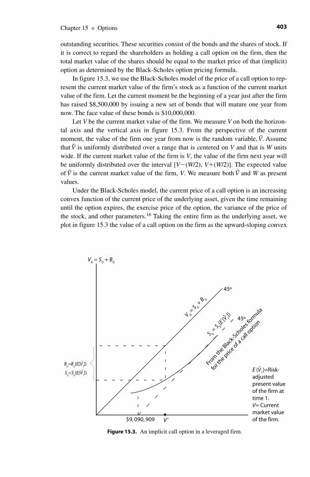
outstanding securities. These securities consist of the bonds and the shares of stock. Ifit is correct to regard the shareholders as holding a call option on the firm, then thetotal market value of the shares should be equal to the market price of that (implicit)option as determined by the Black-Scholes option pricing formula.

In figure 15.3, we use the Black-Scholes model of the price of a call option to rep-resent the current market value of the firm’s stock as a function of the current marketvalue of the firm. Let the current moment be the beginning of a year just after the firmhas raised $8,500,000 by issuing a new set of bonds that will mature one year fromnow. The face value of these bonds is $10,000,000.

Let V be the current market value of the firm. We measure V on both the horizon-tal axis and the vertical axis in figure 15.3. From the perspective of the currentmoment, the value of the firm one year from now is the random variable, V. Assumethat V is uniformly distributed over a range that is centered on V and that is W unitswide. If the current market value of the firm is V, the value of the firm next year willbe uniformly distributed over the interval [V�(W/2), V�(W/2)]. The expected valueof V is the current market value of the firm, V. We measure both V and W as presentvalues.

Under the Black-Scholes model, the current price of a call option is an increasingconvex function of the current price of the underlying asset, given the time remaininguntil the option expires, the exercise price of the option, the variance of the price ofthe stock, and other parameters.16 Taking the entire firm as the underlying asset, weplot in figure 15.3 the value of a call option on the firm as the upward-sloping convex


V 0 =

S 0 +

B 0

V0 = S

0 + B

0

From

the Black

-Sch

oles form

ula

for t

he pric

e of a

call o

ption

S 0 =

S 0(E

[V 1])

45º

45º

˜E (V1)=Risk-

adjusted present value of the firm at time 1.V= Current market value of the firm. $9, 090, 909

S0=S

0(E[V

1])

B0=B

0(E[V

1])

˜

˜

˜

V ’

Figure 15.3. An implicit call option in a leveraged firm.

curve, S0 � S0(E[V1]). Since we regard the stockholders as a group as having a calloption on the entire firm, the height of S0�S0(E[V1]) is the current aggregate marketvalue of the stock as a function of the current market value of the firm. The marketvalue of the firm is equal to the sum of the market values of the firm’s outstandingsecurities. Then for any value of V, the height of the 45° line from the origin abovethat value of V is equal to the sum of the current market values of the stocks and thebonds. Consequently, for any current value of the firm on the horizontal axis, the ver-tical difference between the height of S0 � S0(E[V1]) and the 45° line from the originis the current market value of the firm’s bonds.

Let V be a specific value for V. Then the range of values for V is the intervalbetween the points V�(W/2) and V�(W/2) on the horizontal axis in figure 15.3. Thepresent value of the maturity value of the bonds is $10,000,000/[1 + .10], or$9,090,909. If the (present value of the) outcome next year for V lies within the sub-interval [V�(W/2), $9,090,909], the shareholders will default on the bonds becausethe value of the firm will be less than the maturity value of the bonds. Using the termi-nology of options, the exercise price of the option will exceed the value of the asset onwhich the option is written. Consequently, the holder of the option will allow it toexpire unexercised. Alternatively, if the value of V lies in the subinterval ($9,090,909,V�W/2), the shareholders will exercise their option to purchase the firm by payingoff the bonds.

The fact that the shareholders will finance the payment to bondholders in part byissuing new bonds is irrelevant. The critical consideration is that the shareholders will“purchase” the firm from the bondholders by paying the maturity value of the bonds.

It is easy to understand why the height of the curve increases as the current mar-ket value of the firm increases. The height of S0�S0(E[V1]) is the current value of theimplicit option held by the shareholders. For any current market value of the firm, thevalue of the option is the expected value of the difference between the value of thefirm next year and the maturity value of the bonds.17 This difference is a uniformlydistributed random variable whose expected value is equal to the current value of thefirm, V. An increase in the expected value shifts this distribution rightward. Since thematurity value of the bonds is fixed, any rightward shift of the range of the distribu-tion of V increases the range of positive values for the difference between the futurevalue of the firm and the maturity value of the bonds. Consequently, an increase in thecurrent value of the firm increases the current value of the implicit call option, andthus the curve S0�S0(E[V1]) has a positive slope.

The lower of the two 45° lines in figure 15.3 begins on the horizontal axis at$9,090,909, which is the present value of the maturity value of the bonds. At thispoint, the height of the upper 45° line is $9,090,909. Since the two 45° lines are paral-lel, the vertical distance between them is $9,090,909 for any value of V�$9,090,909.

As the current value of the firm increases, the curve S0�S0(E[V1]) approaches thelower 45° line, becoming coincident with that line for V�$9,090,909�W/2. WhenV�$9,090,909�W/2, the lower bound of the distribution for V is at least as large as thepresent value of the maturity value of the bonds. Once the current value of the firm ishigh enough so that there will be no default on the bonds, the value of the option isequal to the value of the firm minus the present value of the maturity value of thebonds. Moreover, once V�$9,090,909�W/2, each further $1 increase in the current


value of the firm increases the value of the shareholders’ implicit option by the sameamount. Consequently, for all values of V that exceed $9,090,909�W/2, the bonds areriskless.

Finally, we assert without proof that for any value of V, the slope of the S0�

S0(E[V1]) curve is the probability that the shareholders will exercise their option byredeeming the bonds on schedule.18 As we explained earlier, if V is less than$9,090,909�W/2, there is a positive probability of default. Accordingly, for V

$9,090,909�W/2, the slope of S0�S0(E[V1]) is less than 1. As V increases, the pro-portion of the distribution for V that lies to the left of $9,090,909 decreases, thusreducing the probability of default. Accordingly, as V increases, the slope ofS0�S0(E[V1]) increases. Once V reaches $9,090,909�W/2, the probability of defaultreaches 0, and the slope of S0�S0(E[V1]) becomes equal to 1.

The Black-Scholes option pricing formula provides valuable information aboutthe equilibrium prices of the securities of a leveraged firm. By regarding the commonstock as an implicit option, we can determine the equilibrium allocation of the totalvalue of the firm between the shareholders and the bondholders. Moreover, we candetermine the probability of default on the bonds. Of course, to do this we must esti-mate the values of the parameters required by the Black-Scholes formula. One ofthese required parameters is the variance of V, the future value of the firm.

15.10 An Implicit Option on a Postponable and Irreversible Investment Project

15.10.1 The Model

The ES&D Railroad has an opportunity to construct a branch line that would run 10 miles from its main line to a new factory being constructed now, at time 0, in anisolated rural area by the Genteel Furniture Company. The construction of the factorywill be completed one year from now, at time 1. Construction of the branch line wouldrequire one year.

The managers of the furniture company plan to ship large quantities of roughlumber to the factory from distant locations, produce an unusual line of new furniture,and ship it to retail stores across the country. For a variety of reasons, the owners ofthe factory prefer to use the railroad to receive the raw materials and to ship the fin-ished goods, assuming that the branch line is available. Shipping and receiving bytrucks is an alternative because the factory is located 100 miles from an interstatehighway.

The managers of the furniture company are reasonably certain that the demandfor the new product will be strong enough to justify having constructed the factory.There is, however, a chance that the new line of furniture will flop. To reduce theirrisk, the managers will use the coming year to conduct test marketing of some samplesof the new furniture. If the results are positive, the managers will begin producing thenew line of furniture in the new factory at time 1. If the results are negative, the man-agers will sell the newly completed factory. There are no other plants located near theproposed branch line of the railroad, and there is little prospect that a new owner of theplant would use the branch railroad line.


The railroad is assured of a sufficient volume of traffic to justify constructing thebranch line if the demand for the new line of furniture is as strong as the managers ofthe Genteel Furniture Company expect. But if the new line of furniture flops, the rail-road will earn nothing on its investment in constructing the new branch line.

The managers of the ES&D Railroad have a choice:

1. Construct the branch line immediately so that it is ready for use by the timethat the furniture company is ready to begin operations at its new factory.

2. Postpone for one year the decision on constructing the branch line. If theGenteel Furniture Company begins to operate their new factory at time 1 (hav-ing learned from their test marketing that the demand for the furniture will bestrong), begin construction of the branch line at time 1. Otherwise, do not con-struct the line.

Each choice is risky.Constructing the branch line at time 0 is risky because the new line of furniture

might flop, in which event the railroad would earn nothing on its investment.Postponing a decision on constructing the branch line is also risky. Without the

new branch line in place when the factory begins operations, the managers of the fac-tory will use trucks to receive lumber and to ship furniture during the first year ofoperation. Once the trucking companies begin serving the new factory, they might beable to provide incentives that would overcome the managers’ preference to ship byrail. In this event, the railroad might have to offer a substantial discount to persuadethe managers to switch from trucks to rail. The discount would reduce the rate ofreturn on the railroad’s investment in constructing the branch line.

The railroad’s opportunity to construct the branch line has the characteristicsrequired for an implicit option. First, the railroad can postpone its decision on con-structing the line. Unlike some investments, the opportunity to construct the line is nota now-or-never proposition.

Second, there is no salvage value for the investment because there is littleprospect that there will be other customers for the railroad on the new branch line.Should the railroad construct the new line, the value of the resources committed tothat construction would be irrecoverable.

Third, at time 0 the net present value of an investment in the branch line is uncer-tain because no one knows how consumers will respond to the new line of furniture.

It is easy to see the analogy between the railroad’s prospective investment and acall option on a stock. An investor who owns a call option on IBM common stock hasthe flexibility to postpone the decision on acquiring the stock at the fixed exerciseprice, E, in order to collect additional information. Of course, the investor cannotretain this flexibility beyond the expiration date of the option.

The current value to the investor of the flexibility to postpone the decision is thecurrent market price of the option. Were this not so, a rational investor would sell theoption rather than continue to hold it.19

An investor who acquires the stock now will pay two costs; one is explicit, theother is implicit. The explicit cost is the exercise price of the option. The implicit costis the current market price of the option.


Once the investor exercises the option, he or she will own the stock for better orworse; the investor will no longer have the opportunity to postpone the decision inorder to consider additional information. Consequently, to exercise the option now isto destroy an opportunity whose value is the current market price of the option.

The railroad has an option to obtain the new branch line (by constructing it). Thebranch line is analogous to the IBM stock; both assets are claims to uncertain futuresequences of payments. The exercise price of the railroad’s option to acquire the newbranch line is the cost of constructing it.

The railroad’s option on the new branch line has a value. In principle, we couldimagine a market in which the railroad could sell its option to construct the branch line.If such a market existed, the railroad’s option on the new branch line would have a mar-ket price, and this price would be the implicit component of the cost that the railroadwould incur to acquire the new branch line. In fact, it is unlikely that there would be anorganized market in which the railroad’s option on the branch line would be traded.Consequently, there will be no market price for the option. But the absence of an organ-ized market for the railroad’s option does not mean that the option has no value. Thechallenge is to use option pricing theory to estimate the value of the option so that therailroad can more accurately calculate the net present value of acquiring the branchline. More accurate calculations of the net present values of prospective investmentprojects lead to a more efficient allocation of resources.


We will now present a simple numerical model of the railroad’s implicit option on theinvestment project defined as constructing the proposed branch rail line. The revenuesfrom hauling freight on the branch line depend on whether the test marketing of thenew furniture is successful and on whether the branch line is ready for traffic when thefurniture company begins to operate its new plant. Constructing the branch linerequires one year. The railroad could begin to construct the branch line at time 0. If thetest marketing of the new furniture between time 0 and time 1 succeeds, the furniturecompany will begin shipping by rail at time 1, and the railroad will receive annual rev-enues equal to $3,000,000 beginning at time 1 and continuing forever. If, however, thetest marketing of the new furniture fails, the furniture company will not operate theplant, and the railroad will receive nothing.

Alternatively, the railroad could postpone the decision on constructing the branchline until time 1, when the furniture company will have the results of the test market-ing of the new furniture. If the new furniture succeeds, the furniture company willbegin to operate its new plant at time 1 and ship by truck. If the railroad then beginsconstruction of the new branch line, it will be ready for traffic beginning at time 2, andthe railroad will obtain annual revenues of $2,800,000 beginning at time 2 and contin-uing forever. The reduction in the annual revenues reflects the discount required topersuade the furniture company to switch its shipping from truck to rail. If the newfurniture is not successful, the railroad will not begin to construct the proposed branchline. The (explicit) cost of construction is $20,000,000, which the railroad must pay atthe beginning of the year in which the construction occurs.


The railroad’s subjective probability that the new line of furniture will succeed is.8. The prospective revenues from freight traffic on the new branch rail line are uncor-related with the performance of the macroeconomy. Hence, the systematic risk of theinvestment project is zero, and we can use the rate of return on the risk-free asset to cal-culate the net present value of the project. The risk-free rate of return is .10 per year.

The railroad has an implicit option to purchase the new branch line. The exerciseprice of the option is $20,000,000. The option has value because it allows the railroadto postpone its decision on purchasing the branch line pending additional informationabout the profitability of that line. Since there will be no additional information avail-able beyond time 1, and thus no point in postponing any further the decision on con-structing the branch rail line, the option expires at time 1. To begin constructing thebranch line at time 0 is to kill the option to collect additional information. Conse-quently, the net present value of a decision to begin construction today should reflectthe opportunity cost of killing the option.

To understand this, let V0(0) be the net present value (as of time 0) of a decisionto begin construction of the branch at time 0, ignoring the opportunity cost of killingthe option. Using the conventional calculation of net present value, we have:

(15.25)

In words, if the railroad begins construction at time 0, it incurs a cost of$20,000,000. With a probability equal to .8, the new line of furniture will succeed, andthe railroad will obtain annual freight revenues equal to $3,000,000, beginning at time 1 and continuing forever. The net present value of this sequence would be$3,000,000/.10, or $30,000,000, if the revenues were certain to occur. But since therevenues will occur only with a probability of .8, the expected net present value of therevenues is only (.8)$30,000,000, or $24,000,000. The railroad pays the constructioncost with certainty at time 0. Then the expected net present value of beginning con-struction of the branch line at time 0 is �$20,000,000�$24,000,000, or $4,000,000.

To maximize its shareholders’ wealth, the railroad should undertake every projectthat has a positive net present value. Since V0(0) is positive, the railroad should beginconstruction of the branch line at time 0. We will now show that this conclusion isincorrect because the calculation of the net present value in equation (15.25) ignoresthe cost of killing the implicit option.

Let V0(1) be the net present value (as of time 0) of a decision to begin constructionat time 1 if the furniture company begins to operate its new plant at time 1. We have:

With probability of .8, the railroad pays $20,000,000 at time 1 to begin constructionof the branch line. Annual revenues of $2,800,000 begin one year later, at time 2, and

V0 (1) (.8)[ $20,000,000 ($2,8000,000/.10)]/(1 .10)

(.8)( $

� � � �

� � 220,000,000 $28,000,000)/(1 .10)

(.8)(8,000,000)/(1 .10)

(

� �

� �

� ..8)$7,272,727

$5,818,182.�

V0 (0) $20,000,000 (.8)($3,000,000/.10)

$20,000,000 $24,0

� � �

� � � 000,000

$4,000,000.�


(15.26)

continue forever. The present value of these revenues as of time 1 is $2,800,000/.10, or$28,000,000. Then the net present value of the project as of time 1 is $8,000,000.Dividing $8,000,000 by (1�.10) produces the present value as of time 0. Finally, multi-plying by .8 adjusts the net present value for the fact that the railroad will construct thebranch line only if the test marketing of the new line of furniture is successful.

Equation (15.25) states that if the railroad begins construction of the branch lineat time 0, the expected value (as of time 0) of the increase in the shareholders’ wealthwill be $4,000,000. From equation (15.26), the expected value (again as of time 0) ofthe gain for shareholders of delaying the decision on construction until time 1 is$5,818,182. Since the two projects are mutually exclusive, the railroad should choosethe second one.

We can restate the railroad’s opportunities in terms of two options. For eachoption, the underlying asset is the new branch line to be delivered one year after theoption is exercised, and for each option the exercise price is $20,000,000, which is thecost of constructing the new line. The first option expires now, at time 0; the secondoption expires one year from now, at time 1. At time 0, the value to the railroad of thefirst option, the one that will expire momentarily, is $4,000,000. In chapter 3 weexplained that the net present value of a project is the maximal amount of money thata firm would be willing to pay for the right to undertake the project.20 By beginningconstruction of the branch line now, the railroad would increase the expected value ofits shareholders’ wealth by $4,000,000.21

But the value to the railroad at time 0 of the option that will not expire until time1 is $5,818,182. To maximize its shareholders’ wealth, the railroad should be willingto pay up to $5,818,182 for the right to postpone for one year the decision whether topurchase the (construction of the) new branch line for $20,000,000. As we learnedearlier in this chapter, increasing the time remaining until the option expires increasesthe value of the option.

The conventional rule for choosing investment projects is to undertake any proj-ect that has a positive net present value. In equation (15.25), the net present value,V0(0), of the project in which the railroad begins construction now is positive, and yetwe have demonstrated that the railroad’s shareholders will gain wealth if the railroadrejects that project. The anomaly vanishes when we recognize that the calculation ofV0(0) ignores an implicit cost, namely the cost of killing the option to postpone thedecision. The value of this option is $5,818,182. Let V 0 (0) be the net present value ofthe project net of the cost of killing the implicit option. Then

(15.27)

Since the net present value, properly calculated, of beginning construction now is neg-ative, the railroad should reject this project.

We conclude that recognizing implicit options contained in proposed investmentprojects can enable firms and investors to calculate net present values more preciselyand thereby increase the efficiency of the allocation of resources.

′V V0 (0) (0) $5,818,182

$4,000,000 $5,818,182

$1,818,182.

0� �

� �

� �


15.11 Summary

Options are financial securities because they are saleable rights to receive sequencesof payments. We can determine the equilibrium prices of options relative to the equi-librium prices of other securities by using the same principles that govern the prices ofall securities. One of these principles is that in equilibrium the rate of return on a risk-free portfolio must be equal to the rate of return on a risk-free asset. The Black-Scholes formula for the equilibrium price of an option is based on this principle andon the fact that an investor can construct a risk-free portfolio that contains an optionand the underlying stock.

An efficient allocation of resources is one in which there are no further opportu-nities for mutually beneficial exchanges. A necessary condition for effecting theseexchanges is an accurate evaluation of their net present values. The theory of optionpricing contributes to these evaluations because some of the exchanges containimplicit options. A leveraged firm contains an implicit call option for the shareholders.Option pricing theory has implications for the allocation of the firm’s total marketvalue between the shareholders and the bondholders, and for the probability that thefirm will default on the bonds. This information can assist investors in evaluating pro-posed exchanges by improving the accuracy with which the investors estimate the val-ues of the securities that would finance those exchanges.

Investment projects that are both postponable and irreversible also containimplicit options. By increasing the accuracy with which firms can estimate the netpresent values of these projects, option pricing theory can facilitate mutually benefi-cial exchanges, and thus increase the efficiency of the allocation of resources.

Appendix: Continuous Compounding

In this appendix, we sketch the relationship between periodic and continuous com-pounding of the rate of interest.

Let r be the rate of interest per year. If interest is compounded annually, the valueone year from today of an account that is worth $A today will be:

(15.A1)

By extension, two years from today the account will be worth:

(15.A2)

In general, the value of the account t years from today will be:

(15.A3)

Suppose that the interest is compounded semiannually, and let $Yt be the value tyears from today of an account that is worth $A today. Then the value of the accountone year from today will be:

(15.A4)$ $ [1 ( /2)][1 ( /2)]

$ [1 ( /2)] .

1

2

Y A r r

A r

� � �

� �

$ $ (1 ) .X A rtt� �

$ $ (1 ) $ (1 ) (1 )

$ (1 )

2 11 1 1

2

X X r A r r

A r

� � � � �

� �

$ $ (1 ) .11X A r� �



With semiannual compounding, there are two periods during each year in whichthe account earns interest. The rate of interest per period is (r/2).

Over a span of t years there are 2t periods in which the account earns interest.Then the value of the account t years from today will be:

(15.A5)

Now suppose that interest is compounded n times per year, and let $Zt be thevalue of the account t years from today. By analogy with equation (15.A5), we have:

(15.A6)

Continuous compounding is the limit of equation (15.A6) as the number of com-pounding periods per year, n, increases without bound. Let $Vt be the value of theaccount t years from today when interest is compounded continuously. Then

(15.A7)

Problems

1. A call option expires 2 periods from now. Given the following information,calculate the values of the stock at times 1 and 2, and the values of the option at times0, 1, and 2.

S0�$30

U�.25D�.10R�.10Exercise price�$33

2. A call option expires 2 periods from now. Given the following information, arethe options correctly priced at Nodes 2 and 3?

S0�$10

U�.3D�.05Exercise Price�$11R�.10C1

��$2

C1��$.80

If not, what would one do to obtain a riskless profit? How large is the risklessprofit?

3. Use the put-call parity to create at time 0 (a) a homemade put option that willexpire at time 1, (b) a homemade call option that will expire at time 1, and (c) a home-made share.

$ Limit $ [1 ( / )]

.

Y A r n

n

Ae

tnt

rt

� �

�

�

→

$ $ [1 ( / )] .Z A r ntnt� �

$ $ [1 ( /2)]2Y A rtt� �

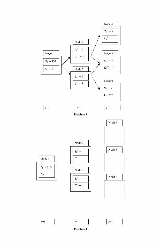
Problem 1

Problem 2

Notes

1. F. Black and M. Scholes, “The Pricing of Options and Corporate Liabilities,” Journal ofPolitical Economy 81 (1973): 637-659.

2. In practice, a call option is usually defined as a right to purchase 100 shares (or some otherconvenient round number). For convenience, and with no loss of generality, we define a calloption as a right to purchase one share.

3. A riskless profit of $1 is trivial, but a riskless profit of $1 per option is not trivial.Purchasing 1,000,000 options and 1,000,000 shares of stock will generate a riskless profit of$1,000,000. We ignore transaction costs.

4. More precisely, competition among investors will reduce the difference between the mar-ket price of the stock and the market price of the option to equality with the difference betweenthe price of the stock and the exercise price of the option, thus eliminating the opportunity for ariskless profit. Whether investors force the price of the option up, or the price of the stock down,or some combination of the two is immaterial for the question at hand. The point is that theequilibrium configuration of the market prices of the stock and the option, relative to the exer-cise price of the option, will provide no opportunity for a riskless profit.

5. We ignore transaction costs.6. The demonstration of this riskless profit is analogous to the numerical example in section

15.2.2 for a call option. We encourage the reader to construct a numerical example for the putoption.

7. The price that Adrian paid to purchase the option prior to time 2 is a sunk cost at time 2.Thus Adrian’s optimal decision at time 2 on whether to exercise the option or allow it to expiredoes not depend on the price that he paid for the option. The level of his profit from having pur-chased the option depends on what he paid for it, but his decision on whether to exercise theoption does not. Compare Adrian’s decision to the irrelevance of a firm’s fixed costs to its opti-mal behavior in the short run.

8. Again for convenience, we assume that investors can trade in fractional units of securities,including options. We could demonstrate our result by having the investor purchase 1,000,000shares of the stock and selling 2,570,000 call options on that stock. Since the ratio is 2.57options sold for each share of stock purchased, the portfolio will be riskless.

9. A detailed numerical example of long and short positions appears in section 8.3.3 of chap-ter 8.

10. Most, if not all, of the intermediate and advanced texts in finance present analyses of thebinomial model of option pricing for N periods.

11. Recall from chapter 7 that the variance of a security’s rate of return is the probability-weighted sum of the squared deviations that are possible between the rate of return and itsexpected value. Whatever the probabilities that govern whether the stock will follow the up pathor the down path from one time to the next, an increase in the values of the up factor and thedown factor will increase the variance of the stock’s rate of return.

12. Recall that this statement does not hold for dates prior to the expiration date.13. The reader might review chapter 11 on the efficient markets hypothesis for the economic

interpretation of immediate.14. More precisely, the opportunity cost of holding the option for one period is equal to the

risk-adjusted interest rate (per period) multiplied by the current market price of the option.15. In practice, because the ownership of the common stock is widely dispersed, individual

shareholders or small groups of shareholders have virtually no control over their managers.Important exceptions occur if mutual funds or pension funds own sufficiently large blocks ofshares. The California State Pension Fund is an example of a fund that frequently affects thedecisions of firms in which it holds investments. In any case, the managers of a firm do have an


interest in increasing the value of the firm’s shares. But (as we learned in chapter 13) problemsof agency can create conflicts between the interests of the managers and the interests of theshareholders.

16. More advanced texts provide a derivation of this statement.17. Subject to the condition that the value of the option cannot be negative.18. Advanced texts in portfolio theory demonstrate this fact.19. More precisely, the market price of the option is the marginal value to the investor of the

right to postpone the decision.20. If future costs and revenues are certain, the shareholders’ wealth will increase by the net

present value of the project, minus whatever the firm pays for the right to undertake the project.Equivalently, we could define the costs of the project to include any fee that the firm must payfor the right to undertake the project.

21. We assume that the railroad operates several investment projects. For example, each reg-ularly scheduled train is a project that involves a sequence of uncertain costs and revenues. Theshareholders are concerned with the expected rate of return and the risk on the railroad’s portfo-lio of projects. If the systematic risks of these projects are zero, the railroad should undertakeany project that has a positive net present value.


16.1 Introduction

A futures contract is a standardized version of a forward contract. A forward contractis an agreement under which one person agrees to deliver a specified quantity of agood to a second person at a specified future time in exchange for a price that is spec-ified when the contract is made. For example, suppose that on March 16, 2005, Mr. Xpurchases a forward contract in oats from Mr. Y. The contract specifies that onSeptember 30, 2005, Mr. Y must deliver one ton of oats to a designated location (suchas Kansas City), and that Mr. X will accept delivery of one ton of oats at that locationand pay $46 to Mr. Y. The $46 is the forward price to which Mr. X and Mr. Y agreedon March 16, 2005, for delivery of oats on September 30, 2005.1

The forward contract described above is a private agreement between Mr. X andMr. Y, who negotiate directly with each other. For most forward contracts, there is noorganized market in which the contracts can be traded continuously over time. Theabsence of an organized market for forward contracts substantially increases the trans-action costs incurred by using forward contracts to effect mutually beneficialexchanges. The higher the transaction costs, the fewer exchanges will occur, with aconsequent decrease in economic efficiency.

There are three ways in which the absence of an organized market for forwardcontracts increases transaction costs. First, both Mr. X and Mr. Y incur considerablecosts to find each other and to negotiate the terms of the contract. Second, each manincurs a risk that the other man will not meet his obligations under the contract. Mr. Xmight refuse to accept delivery of the oats at the agreed price of $46. Similarly, Mr. Ymight refuse to deliver the oats in exchange for $46.

Third, the lack of an organized market substantially increases the costs that eachman would incur to cancel the commitment that he made under the contract, shouldchanges in circumstances make it advantageous for him to do so. For example, afterthe contract is created in March, but before September arrives, Mr. X could decide thathe no longer wants to accept delivery of oats in September and pay $46 per ton. Ifthere were an organized market on which forward contracts were traded, Mr. X couldeasily find a third party, say Ms. Z, who would purchase from him the right to receiveoats in September from Mr. Y, and pay Mr. Y $46 per ton. The price at which Mr. Xcould sell to Ms. Z his right to receive oats from Mr. Y would be set by negotiationbetween Mr. X and Ms. Z. Similarly, should Mr. Y’s circumstances change, he wouldhave an incentive to find a third party, say Mr. W, who, for a price, would agree to

16 Futures Contracts

415

perform Mr. Y’s obligation to deliver oats to Mr. X in September and accept $46 perton in payment.

By increasing the costs incurred to reverse a position in a forward contract, theabsence of an organized market increases the risk of entering into these contracts,thereby reducing the extent to which these contracts can promote mutually beneficialexchanges.

There is an additional deleterious effect on economic efficiency of the absence oforganized trading in forward contracts. As we have stressed in earlier chapters, mar-kets generate information about possibilities for mutually beneficial exchanges andtransmit this information through prices. The prices at which persons agree to receiveand deliver oats at a future date contain information about future events. As time pro-gresses, there can be new information about these future events. An organized marketwould transmit this new information by promoting continuous trading in forwardcontracts.

A futures contract is a standardized forward contract that is traded continuouslyon an organized market, often known as a futures exchange. The exchange definesseveral kinds of contracts by specifying the commodities to be delivered, the qualityof the commodity acceptable for delivery, where the commodity is to be delivered,and the date on which delivery is to occur. For example, the Chicago Board of Tradeorganizes trading in corn futures that have delivery months of March, May, July,September, and December. The corn may be delivered at Chicago, Burns Harbor,Toledo, or St. Louis.2 The Chicago Board of Trade (with its affiliated organizations)also guarantees the performance of investors who buy or sell these contracts. Using aprocess called marking to the market, the Board of Trade causes the prices of futurescontracts to reflect new information about future events. We will explain the processof marking to the market in section 16.6.2.

Markets for futures contracts promote economic efficiency by allocating riskamong persons according to their comparative advantages in bearing risk. When theeconomy allocates resources according to comparative advantage, the economyexpands the set of achievable mutually beneficial exchanges. In this chapter, weexplain how markets for futures contracts promote mutually beneficial exchangesamong producers, speculators, and consumers.

16.2 Futures Contracts as Financial Securities

In section 2.1 of chapter 2, we defined a financial security as a saleable right to receivea sequence of future payments. The practice of marking to the market makes a futurescontract a financial security. “A futures price is something of a misnomer, for it is nota price at all. Rather, purchasing or selling futures contracts means making a legalcommitment to accept a series of cash flows called variation margin during the periodthe contracts to deliver (or accept delivery) are held.3 A futures exchange maintains anaccount for each investor who purchases or sells a futures contract on that exchange.Investors are required to deposit with the exchange an amount of money, called a mar-gin, to increase the likelihood that they will meet their obligations to deliver, or to


accept delivery, as specified by the contracts that they have purchased or sold. Thevariation margin is the amount by which the exchange adjusts the investor’s accountas the contracts are marked to the market.4

16.3 Futures Contracts and the Efficient Allocation of Risk

To achieve economic efficiency, the economy must do more than allocate the produc-tion of oats to those farmers who have a comparative advantage in producing oats. Theeconomy must promote an efficient specialization and exchange in every aspect of theproduction of oats. For example, farmers who grow oats do not also produce the fertil-izer that they use. Nor do they manufacture the tractors that they use, any more thanthey refine the gasoline that they use in their tractors. In an efficient allocation ofresources, those persons who have a comparative advantage in the planting and har-vesting of oats do only that; the production of fertilizer, tractors, and gasoline is left topersons whose comparative advantages lie in the production of those goods.

One aspect of the production of oats is the risk that farmers will overestimate in thespring, when they decide how much oats to plant, the price at which they will be able tosell the crop in the fall. An efficient allocation of resources will assign this risk to who-ever has a comparative advantage in bearing it. It is plausible that farmers will not havea comparative advantage in bearing risk; their specialty is in determining how to com-bine land, seed, fertilizer, machinery, and time to produce oats. They are not skilled inpredicting the price of oats several months in advance. But there are persons who dospecialize in predicting future values of the price of oats. Some of these persons, calledspeculators, sell their knowledge to farmers through the process of insulating farmersfrom the risks involved in predicting the price of oats. A market in futures contracts foroats organizes this mutually beneficial exchange between farmers and speculators.

Suppose that Mr. Green is a farmer who produces oats. Mr. Green calculates thathe will be able to obtain a profit by planting oats in the spring if he can sell the oats forat least $46 in September. Since the price of oats in September might be less than $46,Mr. Green will incur the risk of a loss by planting oats in the spring. He can transferthis risk to a speculator by selling to him on March 16, 2005, a futures contract for thedelivery of oats for $46 on the following September 30. As the purchaser of thefutures contract, the speculator is committed to accept delivery in September, and paythe $46 on which he and Mr. Green agreed in March. Consequently, the speculatorwill bear the risk that the price of oats in September will be less than $46. The specu-lator’s profit (or loss) in September is the difference between the price at which he canresell the oats in September and the $46 that he is committed to pay for it.

Speculators are just as eager as anyone else to avoid losses. Therefore, specula-tors will purchase futures contracts in March for $46 only if they are reasonably surethat the price at which they will be able to sell oats in September will be greater than$46. If speculators have a comparative advantage relative to farmers in predicting thefuture price of oats, the speculators will incur losses less frequently than farmers wouldif they were to predict the future price of oats. A market for futures contracts in oatsdoes not eliminate the risk involved in predicting the future price of oats. Rather, the

Chapter 16 ■ Futures Contracts 417

market enables farmers to transfer that risk to speculators who, because of their com-parative advantage in predicting future prices, can bear the risk at a lower cost than thefarmers can.5

There is an analogous risk for persons who use oats as an input for production.Ms. Black could be a miller who signs a contract in March 2005 to deliver cereals at a fixed price to a chain of hotels for several months beginning in October 2005. IfMs. Black purchases in March the oats that she will require beginning in October, shewill incur storage charges for six months.6 Suppose that Ms. Black calculates that she can make a profit if she can purchase oats in September for no more than $46. Ifthe price of oats in September is greater than $46, she will incur a loss in producingcereals for the hotels at the price agreed to in March.

Ms. Black can transfer this risk to a speculator by purchasing from him a futurescontract for the delivery of oats for $46 on the following September 30. As the sellerof the futures contract, the speculator is committed to deliver oats in September andaccept in payment the $46 on which he and Ms. Black agreed in March. Then thespeculator will bear the risk that the price of oats in September will be greater than$46. The speculator’s profit (or loss) in September is the difference between the priceat which he purchases the oats in September in order to make delivery to Ms. Black,and the $46 that he is committed to accept from Ms. Black for the oats.

We have seen how farmers and speculators, and millers and speculators, can usefutures contracts to effect mutually beneficial exchanges. Consequently, through theintermediary participation of speculators, the farmers and the millers create mutuallybeneficial exchanges between themselves.

By reducing the risks that producers would otherwise incur, markets in futurescontracts also create lower prices for consumers. Prices paid by consumers mustcover producers’ marginal costs; otherwise the producers will reduce their rates ofoutput. Conversely, if producers’ marginal cost curves shift downward, the producerswill expand their rates of output, and reduce the prices that they charge consumers.7

In most cases, producers must make commitments well in advance of learning theprice at which they will be able to sell their product and the prices that they willhave to pay for inputs. The unpredictability of these prices is one of the costsincurred by producers. To the extent that producers can use futures markets to trans-fer these costs to other persons who have a comparative advantage in bearing them, the producers can shift their marginal cost curves downward. Consequently,markets for futures contracts reduce prices paid by consumers by creating an efficient allocation of risk.

16.4 The Futures Price, the Spot Price, and the Future Price

It is critical to distinguish among the futures price for oats, the spot price for oats, andthe future price for oats.

A futures price for oats is a price at which a buyer agrees to deliver, and a selleragrees to receive, oats at a specified future date. The futures price is a fixed numberthat is specified in the futures contract.


The spot price of oats is a price at which a buyer agrees to deliver, and a selleragrees to receive, oats immediately, that is to say, on the spot.

The future price of oats is the value that the spot price will take on a future day.Consider the following example. On March 16, 2005, there are three contracts

available for the delivery of oats. The first contract specifies immediate delivery of theoats; the second contract calls for delivery on June 30, 2005; and the third contractrequires delivery on September 30, 2005. On March 16, 2005, there are three separatemarkets operating simultaneously. Each market corresponds to one of the deliverydates, and each market has its own demand for, and supply of, oats for delivery on thedate that corresponds to that market.

On March 16, the spot market organizes trading between persons who offer tosell, and persons who offer to buy, oats for immediate delivery. On the same day, thesecond market organizes trading between persons who offer to deliver oats on June30, 2005, and persons who offer to accept delivery of oats on that date. The trading inthis market determines the price as of March 16, 2005, of oats for delivery on the fol-lowing June 30. The expression for this futures price is the June (30, 2005) oat futuresprice on March 16.

Finally, the third market determines the price as of March 16, 2005, of oats fordelivery on the following September 30. This price is the September oat futures priceon March 16.

The future (without the s) price of oats for a given future date will (obviously) notbe known until that date arrives.

16.5 The Long Side and the Short Side of a Futures Contract

The two sides of a futures contract are known as the long side and the short side. Fromchapter 10, recall that an investor who holds a long position in a security will gainwealth if the price of the security increases. Conversely, an investor who holds a shortposition will gain wealth if the price of the security decreases. We can easily applythese definitions to futures contracts.

Mr. Green, who sells a futures contract at $46 on March 16 to deliver oats inSeptember, has a short position in the contract. Increases in the value of the spot pricefor oats in September will cause Mr. Green to lose wealth. As the seller of the futurescontract, Mr. Green is committed to deliver oats in September and accept $46 as pay-ment. His profit in September will therefore be $46 minus the cost of delivering the oats.The cost of delivering the oats in September is the spot price in September. To deliveroats in September, Mr. Green must either purchase the oats in September on the spotmarket or draw down his inventory of oats. If he purchases the oats on the spot market,he incurs the spot price as an explicit cost of delivering oats. If he draws the oats out ofhis inventory, he incurs the spot price as an implicit cost because he could have soldthose oats in the spot market. Therefore, his profit in September will be the futures priceat which he sold his contract ($46 in our example) minus the spot price in September.

Suppose that the spot price in September is $44. Then Mr. Green will obtain aprofit of $2 because he will receive $46 for oats that will cost him only $44 to deliver.


If the spot price in September is $49, Mr. Green will incur a loss of $3, because he willincur a cost of $49 to deliver oats for which he will receive only $46. Since the pricethat Mr. Green will receive for the oats delivered in September is the futures price,which is fixed by the contract that he sold on March 16, we conclude that Mr. Green loses wealth as the spot price in September increases. We conclude that thevalue of a short position in a September futures contract for oats varies inversely withthe spot price for oats in September.

Mr. Green’s short position in the futures contract is analogous to an investor’sshort position in a share of IBM stock. The investor is obligated to return one share ofstock to the person (or the broker) from whom he borrowed the share. To deliver ashare back to the broker, the investor must either purchase a share on the open marketor draw a share from his own inventory. In either case, the cost to the investor of deliv-ering the stock is the current price of the stock. As the price of the stock increases, theinvestor who is short in that stock loses wealth.

Ms. Black has a long position in a futures contract. On March 16, she purchaseda contract to accept delivery of oats in September and pay $46 at that time. It is easyto show that the value of a long position in a September futures contract for oats variesdirectly with the spot price for oats in September. Ms. Black can resell in the spot mar-ket the oats that she will receive in September. Her profit will be equal to the spotprice in September minus the fixed price that she is committed to pay for the oats. Thehigher the spot price in September, the higher her profit (or the smaller her loss).

16.6 Futures Contracts as Financial Securities

A financial security is a saleable right to receive a sequence of payments. To show thata futures contract meets this definition, we must explain a bit more about how thesecontracts are traded and how the market determines their prices.

16.6.1 The Clearinghouse

An organized futures market uses a clearinghouse that acts as an intermediarybetween persons who buy and sell futures contracts. The main purpose of the clearing-house is to reduce the risk of buying and selling futures contracts by guaranteeing theperformance of persons who enter these contracts. The use of a clearinghouse isanother example of how a financial market promotes mutually beneficial exchangesby allocating risk among persons according to their comparative advantages in bear-ing risk.

Continuing with our example involving Ms. Black and Mr. Green, on March 16futures contracts for oats delivered on September 30 are trading at $46. Mr. Greenplaces (through a broker) an order to sell a contract, and Ms. Black places an order topurchase a contract. Since the price at which Mr. Green is willing to deliver oats inSeptember is equal to the price that Ms. Black is willing to pay in September for oatsdelivered then, the two orders can be crossed in a single contract. But this contractinvolves risk for each party because the other party might default. When Septemberarrives, Mr. Green might fail to deliver the oats as promised, or Ms. Black might


fail to pay for the oats as promised. Holding a contract with another person, andobtaining that person’s performance under the contract, are not the same thing.Futures contracts promote economic efficiency by allocating risk among personsaccording to their comparative advantages in bearing risk. The greater the likelihoodof defaults on futures contracts, the less useful these contracts will be in allocating therisks of predicting future prices. Consequently, prospective buyers and sellers offutures contracts will be willing to pay something to reduce the likelihood of defaults.

The clearinghouse reduces the likelihood of defaults by acting as an intermediarybetween those who purchase and those who sell futures contracts. Rather than creatinga single contract between Mr. Green and Ms. Black, the clearinghouse creates twocontracts. Mr. Green sells a contract to the clearinghouse, and Ms. Black purchases anoffsetting contract from the clearinghouse. As a seller of a futures contract for $46,Mr. Green must deliver oats to the clearinghouse on the following September 30 andaccept $46, minus a small commission, in payment from the clearinghouse at thattime. Ms. Black, who purchases a futures contract for $46, must accept delivery of theoats from the clearinghouse in September, and pay $46, plus a small commission, tothe clearinghouse at that time. The commissions are the price that the clearinghousecharges for guaranteeing the performances of Ms. Black and Mr. Green.8

If there is no default, Mr. Green will deliver oats in September to a location des-ignated by the clearinghouse, and Ms. Black will accept delivery of the oats at thatlocation. Ms. Black will pay the clearinghouse $46, plus a commission, and Mr. Greenwill receive from the clearinghouse $46, less a commission. Should Mr. Green fail todeliver the oats in September as promised, the clearinghouse will purchase oats on theopen market in September and deliver the oats to Ms. Black, accepting from her a pay-ment of $46, plus commission. There is, of course, no assurance that the clearinghousewill be able to purchase oats in September for $46. Should the price of oats for imme-diate delivery in September exceed the price of $46 on Ms. Black’s futures contract,the clearinghouse will incur a loss.

Similarly, should Ms. Black fail to purchase oats in September as promised, theclearinghouse will purchase the oats that Mr. Green delivers and pay him $46, less thecommission. The clearinghouse will then sell those oats on the open market, incurringa loss if the price of oats in September for immediate delivery is less than the $46 onMr. Green’s futures contract.

16.6.2 Marking to the Market

Marking to the market is a protocol under which each day the futures prices of all con-tracts that have a common delivery date are changed to the futures price on contractsestablished on the current day for that delivery date. Consequently, contracts that havethe same delivery date are interchangeable. This interchangeability facilitates bothtrading in futures contracts and the transmission of new information about the esti-mated spot price on the delivery date.

Consider the following example. On March 16, competition on the futuresexchange sets the futures price for delivery of oats on September 30 at $46. Mr. Greensells a contract and is thereby obligated to deliver oats in September and receive $46 at that time. Ms. Black purchases a contract and is thereby obligated to acceptdelivery of oats in September and pay $46 at that time.9 The futures price of $46 is the


consensus, on March 16, among investors and speculators, of what the value of thespot price will be on September 30.

March 17 is a new day. Competition on the futures exchange on that day will setthe futures price for September delivery of oats based on all the information that wasavailable through March 16, augmented by whatever new information has arrived onMarch 17. Suppose that the futures price for contracts established on March 17 is$49.10 Now the clearinghouse has two sets of contracts to handle. Contracts estab-lished on March 16 have a delivery price of $46; contracts established on the 17 havea delivery price of $49. Indeed, there will be as many sets of contracts as there aredays on which contracts trade for September delivery.

To facilitate trading in futures contracts for delivery in September, on March 17the clearinghouse will change the delivery prices for the contracts established onMarch 16 from $46 to $49. Simultaneously, the clearinghouse will make offsettingadjustments to the financial positions of the persons who sold or purchased contractson the 16. This practice is called marking to the market.11

Mr. Green sold a contract on March 16. Under the terms of that contract, he is com-mitted to deliver oats in September and receive $46 at that time. Once the clearinghousemarks that contract to the price set by the market on the 17th, he is entitled to receive $49in September, a gain of $3. Mr. Green maintains a cash deposit with the clearinghouse.12

To offset the gain created when the clearinghouse marks his contract to the new price of$49, the clearinghouse reduces his cash balance by $3. Consequently, the net price thatMr. Green will receive for oats delivered in September is $49�$3, or $46, which is theprice to which he committed when he sold the contract on March 16th.

Similarly, when Ms. Black purchased a contract on March 16, she made a commit-ment to accept delivery of oats in September and pay $46 at that time. When the clear-inghouse marks her contract to the market on the 17, her commitment is to pay $49 inSeptember. To offset this loss, the clearinghouse will increase her cash balance by $3, sothat the net price that she will pay for the oats in September is $49�$3, or $46, which isthe price that she agreed on March 16 to pay upon receiving delivery in September.

16.7 Futures Contracts as Transmitters of Information about the Future Values of Spot Prices

In an efficient market, the price of a financial security is continuously adjusted toreflect new information about the underlying sequence of payments. In particular,good news will create a capital gain for an investor who owns that security. Theinvestor can realize that capital gain by selling a portion of her now more valuablesecurity. In several earlier chapters, we described this process of realizing capitalgains as creating a homemade dividend. Of course, bad news will impose a capitalloss on the investor.

Futures contracts are financial securities because they are saleable rights to asequence of future payments. The protocol of marking futures contracts to the marketmeans that the prices of these contracts reflect current information about the futurevalues of spot prices. Consequently, investors who own these securities will enjoy


capital gains (or suffer capital losses) as new information arrives about the futurevalue of the spot price.

Consider the following example for Ms. Black, who purchased a contract onMarch 16 for $46. In purchasing that contract, she made a commitment to accept deliv-ery of oats in September and pay $46 at that time. Since Ms. Black can resell on thespot market the oats that she will receive in September, she will make a profit ifthe spot price on September 30 exceeds $46. On March 17, new information about thelikely value of the spot price for oats in September causes the futures price forSeptember delivery of oats to increase to $49. Based on this new estimate of the spotprice in September, Ms. Black stands to make a profit of $3. Because the clearinghousemarks the futures price on Ms. Black’s contract to $49, and makes an offsetting adjust-ment to her cash balance, she need not wait until September to realize the $3 in profit.

At the end of the day on March 17, the clearinghouse marks the contract that Ms. Black purchased on the 16th up from $46 to $49. She is now obligated to pay anadditional $3 for the oats that she will receive in September. To offset this loss, theclearinghouse will increase her cash balance by $3, so that the net price that she willpay for the oats in September is $49�$3, or $46, which is the price that she agreed onMarch 16 to pay upon receiving delivery in September.

On March 16, Ms. Black purchased a contract for September delivery. Once thiscontract is marked to the market on the 17, she is committed to accept delivery of oatsin September and pay $49. Suppose that on the 17th Ms. Black sells a contract forSeptember delivery. Since the futures price on the 17th is $49, she is now committedto deliver oats in September and accept $49 in payment. The clearinghouse could nowcancel her contract to deliver oats against her contract to accept delivery of oats, sinceboth contracts have the same delivery price of $49. Once the two offsetting contractsare canceled, Ms. Black no longer has any commitments to deliver or accept deliveryof oats, but she does have a cash balance of $3 in her account at the clearinghouse. Bywithdrawing this balance on the 17th, Ms. Black can realize on March 17 the capitalgain generated by the new information on the 17th about the likely value of the spotprice for oats in September.

We conclude this section with a comparison of options and futures contracts. Likeoptions, futures contracts are derivative securities, or derivatives. The current price ofa futures contract is derived from investors’ current expectations about what the spotprice will be on the delivery date specified in the contract. Similarly, the current priceof an option is derived from investors’ current expectations about what the price of theunderlying security will be on the expiration date specified in the option. Unlikeoptions, the parties to a futures contract must make delivery, or accept delivery, of theunderlying commodity. The parties to a futures contract do not have an option to allowthe contract to expire unexercised.

16.8 Investment, Speculation, and Hedging

Intelligent discussion of financial markets in the popular press is inhibited by the factthat many persons regard investment with approval, speculation with disdain, and


display little or no understanding of hedging.13 It is particularly unfortunate that spec-ulation is so ill regarded, because speculation is essential to an informationally effi-cient market, and informational efficiency is a necessary condition for the efficientallocation of resources. Sometimes it seems that a person’s willingness to condemn anactivity as speculation varies inversely with that person’s understanding of the finan-cial security under discussion. Hence, one sees trading in futures contracts denigratedas “just a bunch of speculators playing financial bingo.” Or a large and unexpectedchange in a price is “just the work of greedy speculators,” with the implication thatthere is no acceptable reason for the price to change. In this section, we discuss therelationships among investment, speculation, and hedging in the context of economicefficiency. In chapter 14, we examined the consequences of insider trading for eco-nomic efficiency. Our argument reflects the position of Professor Michael Jensen,who stated in 1986, “Arbitragers provide important productive services to investors,and the supply of these services is threatened by the current outpouring of self-right-eousness and legal action in the wake of the Securities and Exchange Commission’sprosecution of [persons] accused of insider trading.”14

16.8.1 Investment

To invest is to allocate resources out of activities that provide goods and services forcurrent consumption, and into activities that will increase the quantities of goods andservices available for future consumption. Examples come quickly to mind. A farmerincreases the time spent clearing new fields and decreases the time spent weeding thefields currently under cultivation. The shareholders in a firm accept a reduction in cur-rent dividends so that the firm can use retained earnings to finance the development ofa profitable new product. Taxpayers accept an increase in taxes so that the governmentcan construct a more efficient air traffic control system.

Investment necessarily involves the accumulation of capital goods, which can beeither tangible, such as a cleared field, or intangible, such as better computer softwareto assist air traffic controllers. Each capital good has an owner, which could be a sin-gle individual, a set of individuals (such as the shareholders in a firm), or the govern-ment (all members of the society). Ownership brings us to speculation.

16.8.2 Speculation

To speculate is to purchase a good in part because of a belief that the price of that goodwill increase, or to sell a good in part because of a belief that the price of that good willdecrease. Consider the following example of a purchase that is, in part, speculative.

A young husband and wife who plan to begin a family five years from now pur-chase a home that is expensive because it has four bedrooms and a large yard, and islocated in an attractive neighborhood with a good school district. Why purchase suchan expensive home now? Why pay the additional property taxes, interest, insurance,utilities, and maintenance on a home that is far larger than two persons will use? Withno children at the moment, what is the benefit of living in a good school district withits attendant high school taxes? Surely it would be more economical to postpone thepurchase of this home for five years and either rent or purchase a less expensive home


in the interim. By purchasing the expensive home now, the young couple is speculat-ing that the price of the expensive home will not only increase within the next fiveyears, but will increase by more than enough to cover the property taxes, interest, andso on that the couple could avoid by postponing the purchase.

A variation of this rationale is the belief that, while the young couple can affordthe down payment on the home today, the price of the home will increase so rapidlywithin the next five years that the couple will no longer be able to afford the downpayment. Of course, by postponing the purchase of the home, the couple could investin the stock market the money that they have accumulated for the down payment. Bydeciding instead to purchase the home now, the couple is speculating that the rate ofreturn on an investment in the stock market over the next five years will be less thanthe rate at which the price of the house will increase.15

Next consider a case in which a consumer speculates that the price of a good willgo down. Mr. Wheeler owns an automobile that has 130,000 miles on the odometer.The vehicle is in excellent condition cosmetically, but Mr. Wheeler is not willing totrust it mechanically any longer for extended trips, so he purchases a new automobile.Should Mr. Wheeler trade his old automobile in for the new one, or should he store theold automobile until it becomes a valuable antique, at which time he can make akilling? If Mr. Wheeler trades his old automobile in for the new one, he is speculatingthat the value of his old automobile will not increase sufficiently over time to justifythe explicit costs of storing it and the implicit cost of not using it as a trade-in.16

“To own is to speculate.”17 To own something is to speculate that its price willincrease sufficiently rapidly (or decrease sufficiently slowly) to justify owning it now,rather than renting it now or purchasing it later.

Most persons earn incomes by specializing in an activity in which they have acomparative advantage. These persons do not purchase a home or trade in an automo-bile solely for the purpose of speculating on the future value of the price. Some per-sons, however, do specialize in collecting and analyzing information about the futurevalues of the prices of certain assets. For example, some persons specialize in predict-ing the value of the spot price for oats in September. Speculators will use theircomparative advantage to purchase futures contracts when the futures price forSeptember delivery is less than the estimate of what the spot price will be inSeptember. If the speculators’ estimates are correct, the futures prices will increase asthe time for delivery approaches, and speculators will obtain a profit on their futurescontracts as those contracts are marked (up) to the market.

Similarly, speculators will sell futures contracts when the futures price forSeptember delivery is greater than their estimate of the future value of the spot price.Again, if the speculators are correct, the futures prices will decrease as the deliverydate approaches, and they will obtain a profit on their futures contracts as those con-tracts are marked (down) to the market.

By speculating in the market for futures contracts for September delivery of oats,those persons who have a sufficiently strong comparative advantage in predicting futurevalues of spot prices for oats produce two services. First, the speculators publish their estimates of the future value of the spot price by trading in futures contracts, thus causing futures prices to reflect those estimates of the future value of the spot price. Second, the speculators enable producers and users of oats to transfer risk.


By purchasing futures contracts from farmers, the speculators guarantee a price at whichfarmers can sell their oats in September, thus insuring farmers against a low price. Ofcourse, when farmers insure themselves against a low price in September by sellingfutures contracts to speculators, the farmers relinquish the opportunity to gain from ahigh price in September. Similarly, by selling futures contracts to millers, speculatorsinsure the millers against having to pay a high price for the oats they will require to pro-duce cereal.

We know that an efficient allocation of resources depends on financial marketsthat are informationally efficient. Speculators increase the informational efficiency ofthese markets. Unfortunately, speculators and speculation have an undeserved reputa-tion as social parasites. The term greedy speculator is almost a redundancy.

16.8.3 Hedging

To hedge is to construct a portfolio that contains at least two assets whose rates ofreturn are negatively correlated, with the consequence that the rate of return on theportfolio is less volatile than it would be if the portfolio contained only one of thosetwo securities. Similarly, an investor would hedge a position in Asset A by holdingthat asset as part of a portfolio that contains some other asset whose rate of return isnegatively correlated with the rate of return on Asset A.

A portfolio is perfectly hedged if the standard deviation of its rate of return iszero. We saw in chapter 8 on portfolio theory that an investor can construct a perfectlyhedged portfolio by allocating funds in the correct proportions between two securitieswhose rates of return are perfectly correlated. If the rates of return on the two securi-ties are perfectly negatively correlated, the investor takes long positions in both secu-rities. If, however, the two securities are perfectly positively correlated, the investortakes a long position in one of the securities and a short position in the other.In chapter 15 we created perfectly hedged portfolios containing a share of stock and acall option written on that stock to derive the formula for the equilibrium configura-tion of the price of the stock, the price of the option, and the interest rate. Since therates of return on the stock and the call option are positively correlated,18 a long posi-tion in the stock must be hedged by a short position in the option if the portfolio is tobe riskless. The converse is also true.

A farmer who has oats in the ground has a long position in oats (because he willgain wealth as the spot price of oats increases and lose wealth as the spot pricedecreases). He can hedge his long position in oats by taking a short position in oatfutures contracts. We saw in section 16.4 that an investor who sells a futures contractholds a short position in that contract (because he will gain wealth as the spot pricedecreases, and lose wealth as the spot price increases). Similarly, a miller who hasmade a commitment to deliver cereals containing oats in the future in exchange for aprice fixed by contract today has a short position in those cereals, and hence a shortposition in oats. The miller can hedge her short position in oats by purchasing an oatfutures contract today.

The production of most goods and services requires time. Consequently, one ofthe costs that the producer incurs is that the spot prices of inputs or outputs can changeunpredictably between the time that people make a commitment to produce a good,and the time that they can sell that good.19 The existence of organized markets for


futures contracts enables producers to reduce their costs by shifting to speculatorssome of the risk created by the difficulty in predicting future values of spot prices. Bydefinition, speculators take unhedged positions in futures contracts. They are willingto take risks because they have a comparative advantage in predicting future values ofspot prices.

Speculators who do not have a comparative advantage in predicting future valuesof spot prices will lose wealth on their unhedged positions. Eventually, these ineptspeculators will cease their activities, either because they become discouraged orbecause they are ruined financially. Speculators who lose wealth do so because theyeither purchase or sell futures contracts at prices that are not compatible with thefuture values of spot prices. Consequently, these inept speculators cause futures pricesto mislead producers. An efficient market will discourage these speculators by impos-ing losses on them. More generally, an efficient market will allocate resources effi-ciently by encouraging each person to specialize in producing those goods or servicesin which he or she has a comparative advantage. This discipline imposed by an effi-cient market applies to speculators, farmers, millers, and everyone else.

16.9 Futures Prices as Predictors of Future Values of Spot Prices

Futures contracts provide a way for hedgers to insure themselves against unfavorablemovements in the future values of spot prices. Persons who construct speculativepositions in futures contracts therefore have an incentive to collect information aboutthe likely future movements in spot prices. A natural question for financial economistsis whether competition among speculators causes the current price of a futures con-tract to be an unbiased estimate of the value that the spot price will take on the deliv-ery date specified in the contract.

This debate is unresolved. The answer depends in complicated ways on the rela-tive sizes of the positions taken by speculators and by hedgers, whether speculators asa group are risk averse, whether the risk created by unpredictable fluctuations in com-modity prices is diversifiable (with the result that speculators should expect no com-pensation for bearing this risk), and the investigator’s choice of an asset pricing modelto explain future prices. Assessing the state of the debate is beyond the scope of thisbook. For an introduction, the reader might consult the work of Stoll and Whaley.20

16.10 Conclusion

Futures contracts are financial securities because they are saleable rights to a sequenceof future payments. Most of these payments occur as capital gains or losses that occuras the futures prices on existing contracts are marked to the market to reflect newinformation about investors’ beliefs about the future values of spot prices. Markets forfutures contracts increase the efficiency of the allocation of resources by promotingmutually beneficial exchanges between hedgers and speculators.

A hedger is an investor who seeks to reduce the risk of unpredictable changes inthe future values of spot prices by taking a long (or short) position in a good and an


offsetting short (or long) position in a futures contract in that good. A speculator is aperson who specializes in collecting information on the probabilities of future valuesof spot prices. The speculator sells information by taking unhedged positions infutures contracts.

Notes

1. A futures contract is usually denominated in some convenient multiple, such as 100 tons ofoats. For convenience, and without loss of generality, we will suppose the futures contract is forone ton of oats. If the date for delivery is not a business day, Mr. Y must deliver the oats on thelast business day preceding the date for delivery specified in the contract.

2. J. C. Hull, Options, Futures, and Other Derivatives, 6th ed. (Englewood Cliffs, N.J.:Prentice Hall, 2006), 25.

3. D. Duffie, Futures Markets (Englewood Cliffs, N.J.: Prentice Hall, 1989), 11.4. We explain in section 16.6.2 how marking to the market generates positive and negative

flows of cash for the investor.5. Consider the analogy between the example here, the simple example in chapter 1, and the

more complex example in section 6.5 of chapter 6 in which two farmers who have different tol-erances for risk effect a mutually beneficial exchange by merging their farms into a single firmthat issues a contractual claim and a residual claim.

6. One form of storage cost is the depletion that might occur due to spoilage.7. Students will recall from their introductory course that under both perfect competition and

monopoly, a downward shift in the marginal cost curve will cause a profit-maximizing producerto expand the rate of output until marginal revenue is again equal to marginal cost. The producercannot sell the higher rate of output without reducing the price paid by the consumer.

8. The clearinghouse also performs other services, such as record keeping.9. These prices are net of commissions, which we will ignore from here on.10. There are several reasons why the futures price for September delivery could increase

from March 16 to March 17. Immediately after the market closed on the 16th, traders couldhave received information that an infestation of insects will reduce the size of the crop availablefor delivery in September, thus increasing the spot price in September. Or Congress might havepassed a bill subsidizing the sale of oats to certain foreign countries, thus increasing the demandfor oats for delivery in September. For whatever reason, if persons expect on the 17th that thespot price in September will be higher than they had expected on the 16th, they will be unwill-ing to agree on the 17th to deliver oats in September for only $46. Similarly, persons looking toacquire deliveries of oats in September will be willing to commit on the 17th to pay more thanthe $46 to which they would have committed on the 16th.

11. More precisely, the process is “marking (the price set for contracts established on the16th) to (the price set by) the market (for contracts established on the 17th).”

12. Alternatively, the clearinghouse might require Mr. Green to deposit $3. The interest thathe will forego by maintaining a deposit with the clearinghouse is one of the opportunity costs oftrading in futures contracts. We ignore this cost in our calculations.

13. An old joke defines the difference between investment and speculation as follows: “WhenI make money in the stock market, that’s investment; when my mother-in-law makes money inthe stock market, that’s speculation.”

14. M. C. Jensen, “Don’t Freeze the Arbs Out,” Wall Street Journal, December 3, 1986, editorial page.


15. Suppose that banks require a down payment of 10%, and the current price of the home is$100,000. The young couple now has $10,000 with which to make the down payment. If theprice of the house increases by 50% over the next five years, the down payment will be$15,000. But if the five-year rate of return in the stock market is sufficiently greater than 50%,the couple would be better served to rent a house for five years and invest their $10,000 in thestock market during that period rather than in the house.

16. Of course, the reason why most persons trade in their old automobiles is that most auto-mobiles deteriorate to the status of scrap, rather than appreciate to the status of antiques.

17. Stated.18. The correlation is not perfectly negative throughout the entire range of values for the

stock because the range of values for the option is truncated at zero.19. Although most services are produced and consumed instantaneously, many services

require that the persons who produce them spend years acquiring sophisticated skills. Think ofperforming violin concerti or cardiac surgery. A person who invests time and money to acquireany of these skills has an unhedged long position in that skill because there might be a decreasein the future demand for those skills. The unanticipated availability of compact discs or newmedication might reduce (but not eliminate) the demand for certain kinds of violinists or sur-geons long after the investor has invested the resources to acquire those skills.

20. H. R. Stoll and R. E. Whaley, Futures and Options: Theory and Applications (South-Western, 1993), especially chapter 5.



The analysis of the economic efficiency of financial markets involves many topics.This introductory treatment in this book omits several of these topics. The followingsections describe briefly the more important of these topics. At the end of the chapterthere is a selected bibliography for readers interested in a more comprehensive (omitsmore challenging) treatment.

17.1 Bonds

In our analysis of financial securities, we concentrated on common stocks, presentingbonds as an alternative way in which investors can hold claims against a firm’s earn-ings and firms can raise capital to finance new projects. We demonstrated how the useof bonds can promote economic efficiency by organizing exchanges between personswho have different tolerances for risk and by mitigating problems of agency betweenthe shareholders and the managers of a firm. There are many additional ways in whichthe use of bonds affects the efficacy of financial markets. For example, there is a sub-stantial literature on the effect of callable and convertible bonds on economic effi-ciency. The contributions to this literature analyze the optimal behavior of firms andinvestors with respect to these bonds. There is also a large empirical literature on therelationship of the rates of return on bonds that have different amounts of time remain-ing until their dates of maturity.

17.2 Initial Public Offerings

Firms frequently raise capital to finance projects by issuing new securities rather thanby relying on retained earnings. The proportion of the firm that the current sharehold-ers will have to cede to the new investors depends on the price at which the firm cansell the new securities. As is the case throughout economics, setting the price at whichthe firm attempts to sell the new securities involves a trade-off. The higher the price,the smaller the proportion of the firm that the new investors will acquire, and thus thewealthier the current shareholders will be once the firm undertakes the new project.

There is, however, a benefit for the firm in selling the new securities at a lowerprice than the firm might otherwise receive. The probability distributions of the

17 Additional Topics in the Economics ofFinancial Markets

431

sequence of returns that an investor will receive from a firm depend both on the firm’scapital structure and on the portfolio of projects that the firm has underway. By issu-ing new securities, a firm changes its capital structure. It is costly for an investor todetermine how the new capital structure will affect future returns. Similarly, by under-taking a new project the firm creates additional uncertainty for investors. A relativelylow price for the new securities encourages speculators to collect information aboutthe firm. In an efficient market, competition among these speculators causes the pricesof all the firm’s securities to reflect the speculators’ information, thus making thesecurities less risky. The reduction in the levels of risk in the firm’s securities willincrease the price at which the firm can sell new securities in the future, which in turnwill increase the profitability of future new investments. Economists have producedmany studies, both theoretical and empirical, of the pricing of newly issued securitiesand the effect of new issues on economic efficiency. Some of these studies involve theeconomics of signaling, which we discuss below.

17.3 Mutual Funds

A mutual fund is a professionally managed portfolio of financial securities. A fundraises capital by creating shares that investors purchase, just as the IBM Corporationdoes. The difference between a mutual fund and IBM is that the mutual fund uses thecapital provided by investors to purchase a portfolio of financial securities, whereasIBM uses the capital provided by its investors to construct and operate a portfolio ofinvestment projects. By generating economies of scale, a mutual fund can operate aportfolio of financial securities at a lower cost than an individual investor could.Moreover, because the mutual fund is professionally managed, the investor might beable to obtain a higher average rate of return, for a given level of risk, by placingassets with the fund than by managing his or her own portfolio. That is, a mutual fundmight enable an investor to obtain a combination of average rate of return and risk thatlies above the capital market line, thus beating the market on a risk-adjusted basis.

Economists have conducted many empirical studies to determine whether man-agers of mutual funds can outperform the market as agents for their investors. Theanswer is clear: after subtracting the expenses of operating the fund, the managers can-not consistently produce results for their investors that outperform the market. In par-ticular, the managers can neither identify mispriced securities nor predict movementsin the rate of return of the market portfolio (after allowing for the expenses incurred inoperating the fund). Empirical studies of the performance of mutual funds were the firsttests of the efficient markets hypothesis. The use of mutual funds to test the efficientmarkets hypothesis involves complicated empirical problems, such as determiningwhether the fund’s managers maintain a constant level of risk in the fund’s portfolio.

17.4 Behavioral Finance

A fundamental postulate in economic analysis is that persons make rational choices. Aperson’s choice is rational if it is compatible both with that person’s values and with


objective facts. The term behavioral finance designates a set of empirical studies offinancial markets that show that investors (at least some of them) make irrationalchoices. Many of these studies show that the irrational behavior is compatible withsome concepts and empirical data from psychology. Consider the following simpleexample of irrational behavior from financial economics.

Mr. Manor states that he prefers more wealth to less wealth. He has an opportu-nity to invest in a project that has a positive net present value, and he can borrow andlend at a bank at the risk-free rate of interest. (For this example, we ignore risk.) Mr. Manor declines to invest in the project, saying that the amount of cash thathe would have to contribute to initiate the project would require too large a reductionin his current expenditures on consumption. Since the project has a positive netpresent value, Mr. Manor could simultaneously finance the project and obtain its netpresent value by borrowing from a bank. Consequently, by undertaking the project, hecould increase his current level of consumption without reducing his levels ofconsumption at any time in the future. Given Mr. Manor’s preferences (for morewealth rather than less), and the fact that he can borrow from a bank to finance aproject that has a positive net present value, his decision to forego the project is notrational.

Richard Thaler and Werner deBondt produced the seminal study in behavioralfinance. These economists documented that the market produces a systematic over-reaction for stocks that are winners or losers. Specifically, portfolios of stocks thathave underperformed the market in one five-year period outperform the market in asubsequent five-year period, and conversely. Thaler and deBondt argue that ifinvestors were rational, competition among them would diminish these overreactionsto a level consistent with the transaction costs that speculators would incur in attempt-ing to exploit them. But the overreactions persist. The literature on behavioral financecontains many other instances of apparently irrational behavior by investors.

17.5 Market Microstructure

Market microstructure is an encyclopedic term that represents the entirety of themechanisms and institutions through which investors trade financial securities. Acomprehensive analysis of the economic efficiency of financial markets must includea study of market microstructure because the level of allocative efficiency that a mar-ket can achieve depends on the quality of information contained in the prices of thegoods that are traded in that market. Prices emerge from trading. Therefore, themicrostructure of a market determines the extent to which that market can allocateresources efficiently.

17.6 Financial Derivatives

The Black-Scholes option pricing formula is a seminal contribution both to theeconomics of financial markets and to the professional management of risk. Following

Chapter 17 ■ Additional Topics in the Economics of Financial Markets 433

the appearance of the Black-Scholes formula in 1973, there has been a rapid develop-ment of options and futures contracts in financial markets. These securities are knownas financial derivatives. Examples of financial derivatives include futures contracts andoptions on interest rates offered by government bonds, foreign exchange rates, and val-ues of stock market indexes, such as the S&P 500. Both individual investors and firmsuse these securities to reduce the risks associated with future commitments. There isnow a large literature of formal models on how these financial futures are priced andhow investors and firms can use them to increase profits. A comprehensive analysis ofthe equilibrium trade-off between expected rate of return and risk in financial marketsrequires a sophisticated understanding of financial derivatives.

17.7 Corporate Takeovers

Corporate takeovers are likely a close second to insider trading as a popular (and pop-ulist) impassioned belief about unfairness in financial markets. Indeed, the wordtakeover of a corporation has a negative connotation. Discussions in the popular pressof corporate takeovers are inflamed further by the use of expressions such as “corpo-rate raiders” who “attack” a corporation by “making a run” at it.

The scholarly literature on corporate takeovers has made four major contribu-tions. The first contribution is to recognize that the managers of a firm are agents forthe shareholders, who own the firm. The job of the managers is to maximize thewealth of the shareholders. What the press typically represents as a takeover of a cor-poration by outsiders is, in fact, the outcome of competition among alternative teamsof managers for the right to manage the shareholders’ assets. The “outsiders” are notraiders who seize control of the corporation from its shareholders. Rather, the share-holders remain in control and exercise their rights of control to replace the currentteam of managers with a new team that is more to their liking.1

Now, a populist might argue that the outsiders are able to force the current man-agement out of office only by purchasing enough shares so that the outsiders (or theiragents) can acquire a majority of the seats on the firm’s board of directors. But the out-siders can acquire shares only by offering prices that are high enough to induce a suf-ficient number of the current shareholders to sell their shares. Current shareholderswho sell their shares do so voluntarily, presumably because these shareholders preferthe money offered by the outsiders rather than continuing to hold a portion of theirwealth in the securities of this firm. Current shareholders who sell to outsiders volun-tarily cede their portion of the control of the firm to the outsiders. The term takeoverdoes not seem compatible with the voluntary sale of their shares by at least some ofthe current shareholders.

The second contribution that economists have made to the analysis of takeovers isto identify the reasons why investors might want to replace the current team of man-agers with a new team. One reason is to mitigate a problem of agency. Sometimes agroup of investors believes that a different team of managers can operate the firmmore profitably. If the current team of managers has the confidence of the current


board of directors, the only way to install the new managers is to purchase a sufficientnumber of shares to gain a majority of the seats on the board. The price that the out-siders will offer to the shareholders to induce them to sell their shares reflects theincrease in profit that the outsiders believe the new managers can produce. It isinstructive to recognize that the outsiders are risking their own money, believing thattheir expectation of a higher profit is correct.

Problems of asymmetric information can create a reason for replacing the currentteam of managers. We recall that asymmetric information between managers andprospective investors can inhibit a firm from financing a profitable new project. Oneway to resolve this problem is to take the firm private. The board of directors candecide to withdraw the firm’s securities from being listed on exchanges that are acces-sible to the public. The firm would then no longer be publicly traded and therefore nolonger subject to the prohibitions against insider trading. For example, a group ofinvestors could acquire a sufficient number of shares to gain a majority of seats on theboard of directors. The new board could then cause the firm to offer a sufficiently highprice to repurchase all the outstanding securities of the firm, except for those ownedby the directors and a small number of large shareholders. With the firm no longerpublicly traded, the managers can reveal private information to the remaining share-holders and thus finance new projects by raising capital from them.

Another way that a firm can finance new projects in the presence of asymmetricinformation is to acquire a second firm whose current operations generate more cashthat it can profitably invest. In effect, each firm becomes a division of a single new firm.The new firm can then finance internally projects generated by one division by using theearnings of the other division. Having access to internal funds eliminates the problemsof raising capital from new investors under conditions of asymmetric information.

The third major area in which economists have contributed to the analysis of cor-porate takeovers is the empirical determination of which parties gain and which par-ties lose in contests for the control of corporations. Using event studies (discussed inchapter 12), economists have established that the shareholders of corporations that aretaken over almost invariably gain wealth. This fact invalidates the populist argumentthat the shareholders in a firm are harmed by the activities of “raiders.” To the con-trary, by replacing the firm’s current managers with new managers, the raiders makethe firm more profitable, which delivers an increase in wealth to the firm’s currentshareholders by increasing the market value of their shares. These event studies sup-port the efficient markets hypothesis by showing that the prices of a firm’s securitiesbegin to increase at the first sign that a group of investors is attempting to take overthe firm. Moreover, these prices fluctuate to reflect information about the probabilitythat the new investors will succeed in acquiring control of the firm. The losers inbattles to replace a firm’s current management are, of course, the current managers.

Several studies have examined the distribution among bondholders and share-holders of the gains from replacing a firm’s management. Some firms make a busi-ness of identifying and acquiring other firms that, in the view of the acquiring firm,would be more profitable with new management. The empirical evidence is that theshareholders of these acquiring firms neither gain nor lose as a consequence of theirfirms’ acquisitions. A commonly accepted explanation for this is that the price of the


acquiring firm’s securities already reflects investors’ expectations of the earnings thattheir firm will generate by its activities in acquiring other firms.

Finally, some economists have produced interesting results of the relationshipsamong the ways in which investors finance a takeover of a firm and the consequencesof that takeover for the current shareholders of that firm. Investors have severaloptions for financing the purchase of a sufficient number of shares to gain control ofthe firm. For example, the new investors can offer cash to the current shareholders.Alternatively, the new investors can offer a contract under which any current share-holder can transfer ownership of shares to the new investors in exchange for receivingnewly issued securities should the new investors succeed in gaining control of thefirm. Shareholders who do not offer their shares to the new investors will receive aless valuable settlement. The contract between the new investors and the shareholderswho offer their shares to the new investors provides in some way for the event inwhich the new investors fail to gain control of the firm.

The means by which new investors finance their attempt to gain control of a firmhas consequences for the capital structure of that firm. Recall from chapter 13 that afirm’s capital structure has, in turn, consequences for economic efficiency. Therefore,the analysis of the financing of a corporate takeover can be conducted in terms of eco-nomic efficiency, just as we did for the several topics considered in this book.

17.8 Signaling with Dividends

In our discussion of capital structure in chapter 13, we explained how asymmetricinformation between the managers of a firm and prospective investors can create aninefficient allocation of resources. We demonstrated how, under some circumstances,a firm can reduce the degree of asymmetry, and thus mitigate the inefficiency, bychoosing the appropriate security to issue to finance a new project. The firm’s choiceof which security to issue credibly transmits the firm’s private information to prospec-tive buyers of the new securities.

A firm’s choice of the kind of security to issue is an example of the general problem of signaling in economics. When there is asymmetric information betweentwo parties who could effect a mutually beneficial exchange in the absence of theasymmetry, both parties have an incentive to find ways to eliminate (or at leastreduce) the asymmetry. When one or both parties has an incentive to mislead theother, or when either party consists of numerous persons, the costs of gathering, ana-lyzing, and verifying information can preclude the exchange, thus creating economicinefficiency.

To maximize the shareholders’ wealth, the firm’s managers must make optimalchoices of which investment projects to undertake and how to finance them. Optimalchoices of investment projects and the ways to finance them require optimal choicesfor transmitting private information to prospective investors. Economists have pro-duced many theoretical and empirical studies of ways in which a firm might use thepayment of dividends to transmit (or signal) credibly the firm’s private informationabout its ability to generate future earnings.


17.9 Bibliographies

17.9.1 Bonds

Hotchkiss, Edith S., and Tavy Ronen. “The Informational Efficiency of the Corporate BondMarket: An Intraday Analysis,” Review of Financial Studies 15, no. 5 (2002): 1325–1354.

Klein, Linda S., and Dogan, Tirtiroglu. “Valuation Process and Market Efficiency for USTreasury Bonds,” Financial Management 26, no. 4 (1997): 74–80.

Lindvall, John R. “New Issue Corporate Bonds, Seasoned Market Efficiency and YieldSpreads,” Journal of Finance 32, no. 4 (1977): 1057–1067.

17.9.2 Initial Public Offerings (IPOs)

Aggarwal, Reena, and Pat Conroy. “Price Discovery in Initial Public Offerings and the Role ofthe Lead Underwriter,” Journal of Finance 55, no. 6 (2000): 2903–2922.

Derrien, Francois. “IPO Pricing in ‘Hot’ Market Conditions: Who Leaves Money on theTable?” Journal of Finance 60, no. 1 (2005): 487–521.

Loughran, Tim, and Jay Ritter. “Why Has IPO Underpricing Changed Over Time?” FinancialManagement (Autumn 2004).

Michaely, Roni, and Wayne Shaw. “The Pricing of Initial Public Offerings: Tests of Adverse-Selection and Signaling Theories,” Review of Financial Studies 7, no. 2 (1994): 279–319.

17.9.3 Mutual Funds

Brown, Stephen J., William Goetzmann, Roger G. Ibbotson, and Stephen A. Ross. “SurvivorshipBias in Performance Studies,” Review of Financial Studies 5, no. 4 (1992): 553–580.

Elton, Edwin J., Martin J. Gruber, Sanjiv Das, and Matthew Hlavka, “Efficiency with CostlyInformation: A Reinterpretation of Evidence from Managed Portfolios,” Review ofFinancial Studies 6, no. 1 (1993): 1–22.

Prather, Larry, and Karen Middleton. “Are N �1 Heads Better Than One? The Case of MutualFund Managers,” Journal of Economic Behavior and Organization 47, no. 1 (2002): 103–120.

17.9.4 Behavioral Finance

De Bondt, Werner F. M., and Richard H. Thaler. “Does the Stock Market Overreact?” inAdvances in Behavioral Finance, ed. Richard H. Thaler. New York: Russell SageFoundation, 1993.

Lee, Charles M.C., Andrei Shleifer, and Richard H. Thaler. “Investor Sentiment and the Closed-End Fund Puzzle,” in Advances in Behavioral Finance, ed. Richard H. Thaler. New York:Russell Sage Foundation, 1993.

Malkiel, Burton. “The Efficient Market Hypothesis and Its Critics,” Journal of EconomicPerspectives (Winter 2003): 59–82.

Shefrin, Hersh. A Behavioral Approach to Asset Pricing. Burlington, MA: Academic Press,2006, chapters 1, 28, 29.

Shefrin, Hersh, and Meir Statman. “The Disposition to Sell Winners Too Early and Ride LosersToo Long: Theory and Evidence,” in Advances in Behavioral Finance, ed. Richard H.Thaler. New York: Russell Sage Foundation, 1993.

Shiller, Robert. “From Efficient Markets Theory to Behavioral Finance,” Journal of EconomicPerspectives (Winter 2003): 83–104.


17.9.5 Market Microstructure

Clarke, Jonathan E., C. Edward, Fee, and Shawn Thomas. “Corporate Diversification andAsymmetric Information: Evidence from Stock Market Trading Characteristics,” Journalof Corporate Finance 10, no. 1 (2004): 105–129.

Harris, Larry. Trading and Exchanges: Market Microstructure for Practitioners. New York:Oxford University Press, 2003.

Hasbrouck, Joel. “Stalking the ‘Efficient Price’ in Market Microstructure Specifications: AnOverview,” Journal of Financial Markets 5, no. 3 (2002): 329–339.

Lipson, Marc L. “Market Microstructure and Corporate Finance,” Journal of CorporateFinance 9, no. 4 (2003): 377–384.

17.9.6 Financial Derivatives

Amram, Martha, and Nalin Kulatilaka. Real Options. Boston: Harvard Business School Press,1999, 3–45.

Bernardo, Antonio E., and Bhagwan Chowdhry. “Resources, Real Options, and CorporateStrategy,” Journal of Financial Economics 63, no. 2 (2002): 211–234.

Dixit, Avinash, K., and Robert S. Pinkdyck. Investment under Uncertainty. Princeton, N.J.:Princeton University Press, 1994, 3–33.

Faff, Robert, and David Hillier. “Complete Markets, Informed Trading and Equity OptionIntroductions,” Journal of Banking and Finance 29, no. 6 (2005): 1359–1384.

Hentschel, Ludger and S. P. Hothari. “Are Corporations Reducing or Taking Risks withDerivatives?” Journal of Financial and Quantitative Analysis 36, no. 1 (2001).

Howison, Sam, and David Lamper. “Trading Volume in Models of Financial Derivatives,”Applied Mathematical Finance 8 (2001): 119–135.

Trigeorgis, Lenos. Real Options. Cambridge: MIT Press, 1996, 1–21.

17.9.7 Corporate Takeovers

Duggal, Rakesh, and James A. Millar. “Institutional Ownership and Firm Performance: TheCase of Bidder Returns,” Journal of Corporate Finance 5, no. 2 (1999): 103–117.

Griffith, John M., Lawrence Fogelberg, and H. Shelton Weeks. “CEO Ownership, CorporateControl, and Bank Performance,” Journal of Economics and Finance 26, no. 2 (2002).

Holderness, Clifford G., and Dennis P. Sheehan. “Raiders or Saviors? The Evidence on SixControversial Investors,” Journal of Financial Economics 14, no. 4 (1985): 555.

Isagawa, Nobuyuki. “Callable Convertible Debt under Managerial Entrenchment,” Journal ofCorporate Finance 8, no. 3 (2002): 255–270.

Jensen, Michael C. “The Efficiency of Takeovers,” The Corporate Board (September/October1985): 16–22.

Jensen, Michael C., and Richard S. Ruback. “The Market for Corporate Control: The ScientificEvidence,” Journal of Financial Economics 11, nos. 1–4 (1983): 5–50.

Kini, Omesh, William Kracaw, and Shehzad Mian. “The Nature of Discipline by CorporateTakeovers,” Journal of Finance 59, no. 4 (2004): 1511–1552.

17.9.8 Signaling with Dividends

Christie, William G. “Are Dividend Omissions Truly the Cruelest Cut of All?” Journal ofFinancial and Quantitative Analysis 29, no. 3 (1994).


Crawfod, Dean, Diana R. Franz, and Gerald J. Lobo. “Signaling Managerial Optimism throughStock Dividends and Stock Splits: A Reexamination of the Retained Earnings Hypothesis,”Journal of Financial and Quantitative Analysis 40, no. 3 (2005).

Gombola, Michael J., and Feng-Ying Liu. “The Signaling Power of Specially DesignatedDividends,” Journal of Financial and Quantitative Analysis 34, no. 3 (1999).

Kaestner, Robert, and Feng-Ying Liu. “New Evidence on the Information Content of DividendAnnouncements,” Quarterly Review of Economics and Finance 38, no. 2 (1998): 251–274.

Peterson, Steven P. “Some Experimental Evidence on The Efficiency of Dividend Signaling inResolving Information Asymmetries,” Journal of Economic Behavior and Organization29, no. 3 (1996): 373–388.

Viswanath, P. V., and Yu Kyung Kim. “Dilution, Dividend Commitments and Liquidity: DoDividend Changes Reflect Information Signaling?” Review of Quantitative Finance andAccounting 18, no. 4 (2002): 359–379.

Note

1. The new team of managers could increase profit in either, or both, of two ways. First, thenew managers could operate the firm’s current projects more efficiently. Second, the new man-agers could discontinue unprofitable projects and initiate new projects that are profitable. Inparticular, the managers could pay out as dividends any earnings that cannot be invested in proj-ects that do not cover the shareholders’ opportunity costs.



18.1 An Overview

The purpose of a system of financial markets is to facilitate mutually beneficialintertemporal exchanges. Financial markets promote these exchanges by organizingtrading in a variety of financial securities. A financial security is a saleable right toreceive a sequence of future payments. Economists assess the performance of any sys-tem of markets against the criterion of economic efficiency. A system of markets iseconomically efficient if it allocates resources so that there are no further opportuni-ties for mutually beneficial exchanges.

The economic analysis of financial markets is a particular application of micro-economic theory. Equilibrium is the fundamental concept in the analysis of a systemof markets. Equilibrium is a configuration of prices and quantities with the propertythat no one, whether a consumer, an investor, or a manager of a firm, has an incentiveto change their current choices about the quantities that they wish to buy or sell.Equilibrium in a system of financial markets is a configuration of the prices and quan-tities of financial securities such that no person has an incentive to restructure his orher portfolio of securities. An investor’s portfolio of securities contains stocks andbonds issued by firms, and options and futures contracts issued by other investors.Each investor constructs a portfolio to obtain the combination of risk and expectedrate of return that he or she most prefers.

A firm’s portfolio of securities consists of the stocks and bonds that the firm hasissued to finance its operations. The configuration of these securities defines thefirm’s capital structure. A firm’s capital structure can affect the wealth of its share-holders in two ways. First, the choice of capital structure can mitigate problems ofasymmetric information that could reduce the shareholders’ wealth by inhibiting thefirm’s ability to finance new projects. Second, a firm can use its choice of capitalstructure to reduce the costs of agency. Shareholders incur costs of agency becausethey cannot costlessly prevent their managers from operating the firm in ways thatwill transfer wealth from the shareholders to themselves. Since firms compete in thefinancial markets to raise capital to finance new projects, an efficient market willcause firms to choose their capital structures to reduce the costs of asymmetric infor-mation and agency.

18 Summary and Conclusion

441

18.2 Efficiency

An efficient intertemporal allocation of resources requires accurate information aboutthe sequences of future payments generated by current and prospective investmentprojects. Consequently, informational efficiency is a prerequisite for economic effi-ciency. Financial securities are claims, however indirectly, on earnings generated byinvestment projects. Consequently, informational efficiency in financial marketsrequires that the current prices of the securities are compatible with all current infor-mation about the investment projects that underlie those securities. Prices are compat-ible with information if there are no opportunities for investors to obtain positive(risk-adjusted) profits. The information that the prices of the securities must contain(to support an efficient allocation of resources) includes the size, the timing, and thenature of the unpredictable variability of those future earnings.

The efficient markets hypothesis is a statement about the informational content ofthe prices of securities. Most information is not freely available; individuals producethe information and incur costs to do so. The financial markets themselves do notcause the prices of securities to reflect information about investment projects.Investors produce information. By submitting (or withholding) offers to buy and sellsecurities, investors cause the prices of those securities to reflect the information. Themaximal level of informational efficiency in a system of financial markets is condi-tional on the costs of producing information about investment projects and the costs oftrading on that information.

The empirical criterion for informational efficiency is the absence of risk-adjustedresiduals that are sufficiently large and predictable to enable an investor to obtain prof-its that exceed her opportunity costs. A risk-adjusted residual for a security is theamount by which the rate of return on that security differs from the sum of the rewardfor waiting and the reward for bearing risk. The efficient markets hypothesis assertsthat the residuals are unpredictable and small (relative to transaction costs). The calcu-lation of the residuals depends on the economist’s choice of asset pricing model.Consequently, any test for informational efficiency is a test of a joint hypothesis regard-ing the behavior of the residuals and the model for calculating those residuals.

18.3 Asset Pricing Models

The seminal asset pricing model is the capital asset pricing model. In the CAPM, thereward for bearing risk by holding Security i is the product of a market price of riskthat applies to all securities and a quantity of risk that is specific to Security i. Thequantity of risk for Security i is βi, which is the slope of line obtained by regressingthe rate of return on Security i against the rate of return on the market portfolio. Themarket portfolio contains all risky securities in proportions equal to the total marketvalues of those securities relative to the sum of the total market values of all riskysecurities. The value of βi is the marginal effect of the rate of return on the marketportfolio on the conditional expected rate of return for Security i. That is, βi is theamount by which the center point of the probability density function for Security i


shifts when the rate of return on the market portfolio increases by one percentagepoint.

The CAPM is a single-factor asset pricing model. The factor is the market portfolio.The purpose of the factor is to measure the quantities of risk in individual securities.

The empirical shortcomings of the CAPM led to a variety of multifactor assetpricing models. A factor is a portfolio of risky securities. Economists choose the fac-tors based on the ability of the model to explain the trade-off between risk andexpected return in individual securities. In a multifactor asset pricing model, the quan-tity of risk in Security i is multidimensional; Security i has a separate quantity of riskfor each of the factors. Analogously to the CAPM, the quantity of risk contained inSecurity i with respect to Factor j is the marginal effect of the rate of return on Factorj on the conditional expected rate of return for Security i. This quantity of risk is meas-ured by βi,j. There is a separate market price of risk for each factor. The market priceof risk for Factor j is λj. The reward for bearing risk by holding Security i is a sum ofproducts, one for each factor. The risk attributable to Factor j incurred by holdingSecurity i the product is λ jβi, j. Although multifactor models perform better than thesingle-factor CAPM, the seminal contribution of the CAPM has survived in the multi-factor models. The quantity of risk contained in a security is the marginal effect of therate of return on a portfolio on the conditional expected rate of return for that security,and the reward for bearing risk by holding Security i is equal to the product of thatquantity of risk and a market price of risk that is independent of Security i.

With a notable exception, the consensus among economists who study financialmarkets is that the efficient markets hypothesis (constrained by the joint hypothesis) issufficiently accurate to preclude systematic opportunities for a typical investor toobtain profits either by searching for mispriced securities or by anticipating majorchanges in the prices of all securities (timing the market). Investors who have acomparative advantage in obtaining information that is not contained in current prices,and in trading on that information, can obtain profits. The existence of such atypicalinvestors is compatible with the fact that producing information and trading on itare costly.

The notable exception to the efficient markets hypothesis is the behavioralschool, which provides some evidence that investors buy and sell securities based onunsupportable projections of recent trends in the rates of return on those securities. Aconsequence of this irrational behavior is that the prices of some securities can divergesignificantly from values that are compatible with information about the abilities ofthe underlying firms to generate earnings.1

18.4 Market Imperfections

An important topic in the economics of financial markets is the nature and the signifi-cance of various market imperfections. A market imperfection is a situation in whichthe market fails to establish an efficient allocation of resources. That is, a market imper-fection precludes mutually beneficial exchanges that would otherwise occur. We exam-ined two kinds of imperfections: asymmetric information between the managers of a

Chapter 18 ■ Summary and Conclusion 443

firm and the investors who hold that firm’s securities, and problems of agency betweenthe managers and the investors.

The managers of a firm usually have better information about the firm’s prospectsthan investors do. This asymmetry of information can inhibit the firm’s ability tofinance profitable projects by selling new shares. The reason is that investors recog-nize that managers can offer new shares only when doing so will transfer wealth to thefirm’s current shareholders from the investors who purchase the new shares.

When a firm sells new shares, it transfers to new investors a portion of the equitypreviously held by the firm’s current shareholders. The proportion of the equity thatthe firm must cede to the new investors depends on the profitability of the firm,including the new project. If the new project is profitable by itself, the total value ofthe equity (the sum of the current shares and the new shares) will increase when thefirm undertakes the project.2 The distribution of this value between the current share-holders and the new shareholders will depend on the proportion of the equity that thefirm transfers to the new investors in order to induce them to finance the project.When there is asymmetric information, prospective new investors will protect them-selves by insisting on acquiring a larger proportion of the firm than they would ifinformation were symmetric. Under some conditions, the proportion of equity that thefirm must cede to the new investors is so large that the current shareholders will losewealth even though the project is profitable. In this event, the firm will not finance theproject by selling new shares. If the firm has no alternative way to finance the project,there will be an inefficient allocation of resources. The project would have enabled thefirm to increase the wealth of both the firm’s current shareholders and the newinvestors who finance the project.

A firm can avoid this inefficiency by using a portion of its earnings to accumulatea stock of idle cash with which to finance new projects, rather than paying those earn-ings to its current shareholders as dividends. An alternative to using its own earningsto accumulate idle cash is to purchase, or merge with, a firm whose earnings exceedthe cash required to finance profitable new projects in that firm. The idle cash insu-lates the firm from choosing either to forgo the profitable new projects or to raise cap-ital from new shareholders under the disadvantages of asymmetric information.

There is a third way in which a firm can avoid the problem created by asymmetricinformation. Under certain conditions, the managers of a firm can crediblytransmit their information to potential investors by offering to sell specific kinds ofsecurities. In this event, the asymmetry of information disappears. Each firm canfinance its projects without imposing losses of wealth on its current shareholders, andthus there is an efficient allocation of resources. To effect this credible signaling ofinformation, there must be a relationship between the profitability of a firm and thekind of security that the firm can use to finance a project without transferring wealthfrom its current shareholders, and investors must understand this relationship. We pre-sented an example in which strong firms could distinguish themselves from weak firmsby using convertible, callable bonds to finance the project. The weak firms would iden-tify themselves to investors by using straight equity to finance their projects.

We turn now to the problem of agency. To maximize the shareholders’ wealth, themanagers must make all of their decisions regarding capital structure, the selection ofprojects, and the financing of those projects subject to the criterion of maximizing the


value of the shares held by the current shareholders.3 The problem of agency is that theshareholders cannot costlessly monitor their managers. Consequently, the managersenjoy some opportunities to pursue their own interests to the detriment of the share-holders. Managers can reduce the shareholders’ wealth by excessive consumption ofperquisites and by reducing the risk, and thereby the expected rate of return, of the firm.

Excessive consumption of perquisites occurs in many forms, including plushoffices, nepotism, and the use of aircraft and lodgings owned by the firm for vacationsvisibly disguised as seminars, to name only a few. The managers can also undertakeprojects that have negative (risk-adjusted) net present values but that provide the man-agers with personal satisfaction. For example, expanding the firm’s line of products oracquiring another firm will increase the size of the enterprise under the managers’control, which might enable them to feel more important and accomplished.

Managers also have an incentive to operate their firms at lower levels of risk thanthe shareholders prefer because managers cannot diversify their wealth across firms aseasily as shareholders can. According to modern portfolio theory, each investor willallocate funds across firms to achieve the most preferred combination of risk andreturn.4 In effect, the investor is diversifying wealth across portfolios of investmentprojects because each firm is a portfolio of investment projects. The composition ofthe firm’s portfolio determines the combination of expected rate of return and risk thatthe shareholders will receive on their investment in that firm. Shareholders can reduce(or increase) the level of risk to which they expose their wealth by changing the allo-cation of their funds across firms. A significant portion of a manager’s wealth is repu-tational capital, which the manager cannot diversify by managing several firmssimultaneously. Consequently, managers have an incentive to choose for their ownfirms a portfolio of projects that is less risky than the shareholders might prefer.

Another form of the problem of agency is the possibility that the firm’s managerswill transfer wealth from the firm’s bondholders to its shareholders by substitutingriskier projects for the projects that the bondholders intended to finance. We describedthis problem of asset substitution in chapter 13.

The several problems of agency inhibit the ability of firms to persuade investorsto finance projects. To the extent that problems of agency prevent firms from financ-ing profitable projects, there will be an inefficient allocation of resources.Competition among firms for investors’ capital should cause firms to choose capitalstructures that will increase their shareholders’ wealth by mitigating problems ofasymmetric information and agency.

18.5 Derivatives

A derivative is a financial security that contains either a right or an obligation to pur-chase or sell another security or a commodity. Derivatives are special cases of finan-cial securities. We discussed options and futures contracts.

The models for determining the price of options are an application of the proposi-tion that in equilibrium the rate of return on a riskless portfolio that contains an optionand the underlying stock must be equal to the rate of return on the risk-free asset. The


pricing of options is a clear example that the analysis of sophisticated securities (orindeed the analysis of many sophisticated questions in economics) begins with theapplication of fundamental propositions presented in the introductory course. In thecase of options, the fundamental principle is that in (perfectly competitive) equilib-rium there are no opportunities to obtain positive profits net of opportunity costs.

We discussed two applications of implicit options. First, the shareholders in aleveraged firm hold an implicit option written by the bondholders; the underlyingasset is the firm itself. Option pricing models have implications for the relationshipbetween the values of debt and equity in leveraged firm, and for the probability thatthe firm will default on its bonds.

There is also an implicit option in an investment project that has an irreversible(sunk) initial cost and that allows the firm to postpone for a limited time its decisionon whether to undertake the project. The option is the right to postpone a decision inorder to obtain additional information on the profitability of that project. The exercise(or strike) price of the option is the initial cost of the project; the underlying asset isthe project itself. To undertake the project before the time for making a decisionexpires is to exercise (or kill) the option to collect additional information.Consequently, the current value of the option is the value of the right to collect addi-tional information, while retaining the right to undertake the project. We can use anoption pricing model to determine the value of the implicit option. The value of theoption then becomes part of the opportunity cost that the firm will incur by choosingto begin the project now.

Our treatment of futures contracts in chapter 16 is more descriptive and less ana-lytical than our presentations in other chapters. We explained how futures contractspromote mutually beneficial exchanges by allocating the risks of adverse changes infuture prices according to the comparative advantages of producers of commoditiesand investors who speculate in those commodities. We emphasized that speculatorsproduce value by producing information about the future values of prices.

18.6 Implications for Public Policy

The analysis of the economics of financial markets has many implications for publicpolicy regarding the regulation of those markets. The fundamental insight is based onthe recognition that financial markets exist to promote mutually beneficial intertempo-ral exchanges. Therefore, to the extent that the objective of public policy is to promotean efficient allocation of resources (rather than to redistribute wealth), the regulation offinancial markets should be evaluated against the criteria of informational efficiencyand economic efficiency. Regulations that make it easier for investors and firms to mit-igate imperfections such as asymmetric information and problems of agency should bepreserved and, if possible, extended. Regulations that inhibit, or prohibit, mutuallybeneficial exchanges that would otherwise occur should be removed.

Insider trading presents a difficult question for public policy. In chapter 14 weexplained how the effect of insider trading on economic efficiency depends on empirical questions such as the relative importance of traders who are insiders, traders


who are informed outsiders, and liquidity traders. We emphasized that attempts toassess insider trading on the basis of fairness are likely to be futile.

18.7 A Final Word

The formal economic analysis of financial markets is a particular application ofmicroeconomic theory. The concepts of equilibrium, opportunity costs, marginalanalysis, and conditions of tangency that are used throughout microeconomic theoryare as relevant to the analysis of financial markets as they are to any set of markets.Much of the analysis is necessarily complicated by the fact that the goods that arepriced in financial markets are claims on uncertain sequences of future payments.Even so, we hope that the reader will appreciate that the application of microeconomictheory to financial markets produces an understanding of these markets that is analo-gous to many of the applications of economic theory presented in introductory coursesin microeconomics.

Notes

1. The leading proponents of the efficient markets hypothesis and the behavioral school areEugene Fama and Richard Thaler, respectively. Both are economists at the University ofChicago.

2. A project is profitable if its (risk-adjusted) net present value is positive.3. If the managers do not issue new shares, maximizing the wealth of the current sharehold-

ers is equivalent to maximizing the current market price of the outstanding shares.4. In the context of the CAPM, each investor will select a point on the capital market line at

which there is a tangency between that line and one of her indifference curves. Since the capitalmarket line is linear and her indifference curves are convex, this point of tangency is unique,and the tangential indifference curve represents the maximal level of utility that that investorcan obtain.



Chapter 1

1. The price of the bond will decrease because there is an increased probability that thefarm will default on its bonds.

2. All consumers would be better off because they have the choice of paying for the furni-ture today or one year from today. The consumers could acquire the furniture today, and depositin a bank today the price of the furniture. One year from today the consumer could withdraw theinitial deposit to pay for the furniture, and spend the accumulated interest.

ABC furniture will benefit if the increase in future revenue from current sales exceeds (1�the rate of interest) multiplied by what the current revenue would have been in the absenceof the offer to allow customers to postpone payments for one year without interest.

3. No; there is an opportunity for a mutually beneficial exchange. Mr. Green can lend $100 to Mr. Brown at a rate of interest greater than 10% but less than 15%. Both parties will bebetter off.

4. Ms. Black can “buy” Ms. White’s farm by agreeing to pay 1,000 tons of apples per yearto Ms. White. Ms. White will still operate her farm, but she will receive 1,000 tons of appleseach year, being insulated from the variations in productivity from one year to the next. Becausegood and bad weather occur with equal probability, Ms. Black’s average yearly production willincrease from 1,500 tons to 3,000 tons.

Ms. Black would hold a residual claim, similar to a common stock. Each year she willreceive the output that remains after she pays Ms. White 1,000 tons of applies. Ms. White wouldhold a contractual claim, which is like a bond.

Chapter 2

1. A convertible bond enables its owner to protect herself against a decline in price of thestock, while also giving her an option to take advantage of a rise in the price of the stock. If the price of the stock rises, the value of the bond will increase because the investor can convertthe bond into a fixed number of shares, the value of which has increased.

2. Suppose that the bonds issued last year have a face value of $1,000 and a coupon rate of 0.05 per year. The firm is obligated to pay to each bondholder $50 per year [(0.05/year) $1,000] until the bond matures, at which time the firm must redeem the bond by paying $1,000 tothe bondholder.

Suppose also that the rate of return last year on securities that are comparable (in the levelsof risk, timing of payments, etc.) to the firm’s bonds was 0.0625 (6¼%). Assume that investorspaid approximately $800 for these bonds last year. The bonds were sold at a discount from theirface value because their coupon rate of 0.05 was less than the 0.0625 that was available by

Answers to Problems

449

purchasing comparable securities. Since the firm must pay $50 per year for each $800 that itobtained from the investors who purchased the bonds, the firm is paying (and bondholders arereceiving) a rate of interest equal to $50/$800, or 0.0625 (6¼%).

More precisely, the price of the bond last year would be somewhat greater than $800because at maturity the bond holders will receive $1,000, not the price that they paid for thebond last year. Since comparable securities were generating a rate of return equal to 0.0625,which is equal to $50/$800, competition among the investors will have forced the price of thebond above $800. Consequently, the firm will pay somewhat less than 0.0625 for funds bor-rowed by issuing bonds. The amount by which the price of the bond will exceed $800 variesinversely with the time that remains until the bond matures.

If the Fed lowers interest rates, the prices of all bonds, whether newly issued or previouslyissued, will rise. If the bonds that the firm issued last year are callable, the firm can cancel thosebonds by paying the bondholders a fixed amount of money that is less than the market price ofthose bonds. The firm can finance this canceling of its bonds by issuing new bonds at the lowerinterest rates generated by the Fed’s action.

3.A. $260�$90�$170, for a strong firm.

$150�$90�$60, for a weak firm.($170�$60)/2�$115�average market value of all firms’ shares[($260�$150�$90)�($150�$50�$90)]/2�$15�average increase in shareholders’wealth per firms.

B. The average value of a firm with the new project (inclusive of the $90 worth of newresources invested in the project) is ($260�$150)/2�$205. New shareholders will not provide$90 of new capital unless they acquire a sufficiently large proportion of the firm to enable them(on average across all firms) to recoup their investment. Since new shareholders cannot distin-guish between strong firms and weak firms, the current shareholders of any firm must cede theproportion 90/205 of its ownership to the new shareholders. The old shareholders will retain theproportion (115/205) of the firm.

Strong firms will not undertake the project by issuing new shares because the firm’s currentshareholders would lose wealth. Conversely, weak firms would attempt to finance the project byissuing new shares because the current shareholders would gain wealth.

C. Strong firms will finance the project by selling bonds, while weak firms will finance theproject by issuing new shares.

Chapter 3

1. The marginal cost to produce 15 units of gum in East Plant is 3 units of pops. Both plantshave a comparative advantage. West Plant has a comparative advantage in producing pops; EastPlant has a comparative advantage in producing gum.

Answers to Problems450

Levels of Wealth (Liquidation Value)

Strong Firm With the Project Without the ProjectOld shareholders (115/205)*($260)�$145.85 $150.

New shareholders (90/205)*($260)�$114.15 $0.

Weak Firm With the Project Without the ProjectOld shareholders (115/205)*($150)�$84.15 $50.

New shareholders (90/205)*($150)�$65.85 $0.

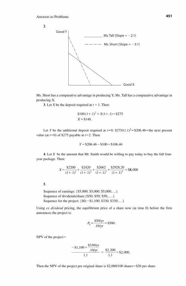
2.

Ms. Short has a comparative advantage in producing Y; Ms. Tall has a comparative advantage inproducing X.

3. Let X be the deposit required at t � 1. Then:

Let Y be the additional deposit required at t�0. $275/(1.1)2�$206.46�the next presentvalue (at t�0) of $275 payable at t�2. Then:

4. Let X be the amount that Mr. Smith would be willing to pay today to buy the full four-year package. Then:

5.

Sequence of earnings: {$5,000; $5,000; $5,000; …}Sequence of dividends/share:{$50; $50; $50;. …}Sequence for the project: {$0;�$1,100; $330; $330; …}

Using ex dividend pricing, the equilibrium price of a share now (at time 0) before the firmannounces the project is:

NPV of the project�

Then the NPV of the project per original share is $2,000/100 shares�$20 per share.

� �

� �

$1,100$330/yr.10/yr

1.1

$2,200

1.1$2,000.

P0$50/yr

.10/yr$500.� �

X ��

��

��

��

�$2200

(1 .1)

$2420

(1 .1)

$2662

(1 .1)

$2928.20

(1 .1)$

1 2 3 488,000

Y � � �$206.46 $100 $106.46

$100 (1 .1) (1 .1) $275

$140.

2� � � �

�

X

X


Good Y

Good X

__________ Ms. Tall (Slope = �2:1)

Ms. Short (Slope = �3:1)

Let P1 be the equilibrium value of the price of a share at t�1 if the firm sells X new sharesat t�1 to finance the project. Then:

The second equation above can be rewritten as:

Using P1 X�$1,100 from the first equation, we have:

or

Then, using P1 X�$1,000, we find:

Hence, the firm must issue (approximately) 2.11 new shares at t�1.The new equilibrium price of a share at t�0 is

Hence, as required, the wealth of the original shareholders increases at t�0 by $20, which is thenet present value of the project per original share.

Chapter 5

(a) {�$5,000,000, �$800,000, �$800,000, �$800,000 ...}(b) The net present value of the project is:

�$5,000,000�([$800,000 per year/0.10 per year)

� �$5,000,000�$8,000,000�$3,000,000.

(c) We recall that the fleet’s regular annual net earnings are $15,000,000. The entire earn-ings are paid as dividends to the 1,000,000 outstanding shares, making the annual dividend pershare equal to $15. Therefore, using an interest rate equal to 0.10, the (ex dividend) price ofeach share is $150.

At time 0 Captain Mo borrows $5,000,000 and purchases the boat. Beginning at time 1 andcontinuing yearly thereafter forever, he will owe $500,000 to the bank as interest on the loan.

PP

01�

�

��

� �

$50

1.1$50 $522

1.1$572

1.1$520.

X � �$1,100

$5222.11 shares.

P1� �$52,200

100$522.

P1��$53,300 $1,100

100,

100 $53,300.P P X1 1� �

P X

PX

1

1

�

��

�

$1,100

($5.000 $330)/yr100.10/yr


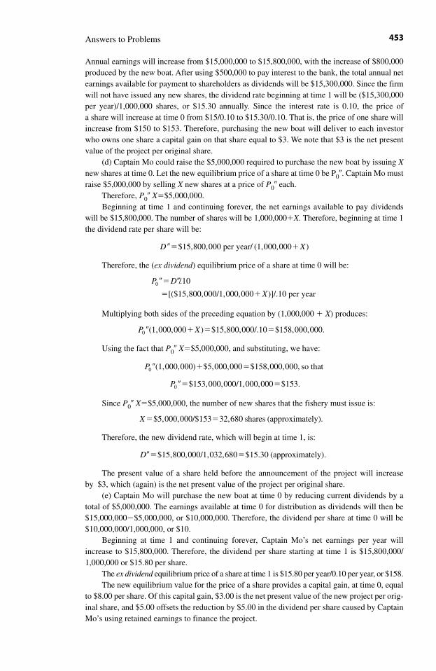
Annual earnings will increase from $15,000,000 to $15,800,000, with the increase of $800,000produced by the new boat. After using $500,000 to pay interest to the bank, the total annual netearnings available for payment to shareholders as dividends will be $15,300,000. Since the firmwill not have issued any new shares, the dividend rate beginning at time 1 will be ($15,300,000per year)/1,000,000 shares, or $15.30 annually. Since the interest rate is 0.10, the price ofa share will increase at time 0 from $15/0.10 to $15.30/0.10. That is, the price of one share willincrease from $150 to $153. Therefore, purchasing the new boat will deliver to each investorwho owns one share a capital gain on that share equal to $3. We note that $3 is the net presentvalue of the project per original share.

(d) Captain Mo could raise the $5,000,000 required to purchase the new boat by issuing Xnew shares at time 0. Let the new equilibrium price of a share at time 0 be P0�. Captain Mo mustraise $5,000,000 by selling X new shares at a price of P0� each.

Therefore, P0� X�$5,000,000.Beginning at time 1 and continuing forever, the net earnings available to pay dividends

will be $15,800,000. The number of shares will be 1,000,000�X. Therefore, beginning at time 1the dividend rate per share will be:

Therefore, the (ex dividend) equilibrium price of a share at time 0 will be:

Multiplying both sides of the preceding equation by (1,000,000 � X) produces:

Using the fact that P0� X�$5,000,000, and substituting, we have:

Since P0� X�$5,000,000, the number of new shares that the fishery must issue is:

Therefore, the new dividend rate, which will begin at time 1, is:

The present value of a share held before the announcement of the project will increaseby $3, which (again) is the net present value of the project per original share.

(e) Captain Mo will purchase the new boat at time 0 by reducing current dividends by atotal of $5,000,000. The earnings available at time 0 for distribution as dividends will then be$15,000,000�$5,000,000, or $10,000,000. Therefore, the dividend per share at time 0 will be$10,000,000/1,000,000, or $10.

Beginning at time 1 and continuing forever, Captain Mo’s net earnings per year willincrease to $15,800,000. Therefore, the dividend per share starting at time 1 is $15,800,000/1,000,000 or $15.80 per share.

The ex dividend equilibrium price of a share at time 1 is $15.80 per year/0.10 per year, or $158.The new equilibrium value for the price of a share provides a capital gain, at time 0, equal

to $8.00 per share. Of this capital gain, $3.00 is the net present value of the new project per orig-inal share, and $5.00 offsets the reduction by $5.00 in the dividend per share caused by CaptainMo’s using retained earnings to finance the project.

D�� $15,800,000/1,032,680 $15.30 (approximately).

X � �$5,000,000/$153 32,680 shares (approximately).

P0 �� $153,000,000/1,000,000 $153.

P0 � � �(1,000,000) $5,000,000 $158,000,000, so that

P X0 � � � �(1,000,000 ) $15,800,000/.10 $158,000,000.

P D

X0 ��

� �

/.10

[($15,800,000/1,000,000 )]/.10 per year

D X�� $15,800,000 per year/ (1,000,000 )


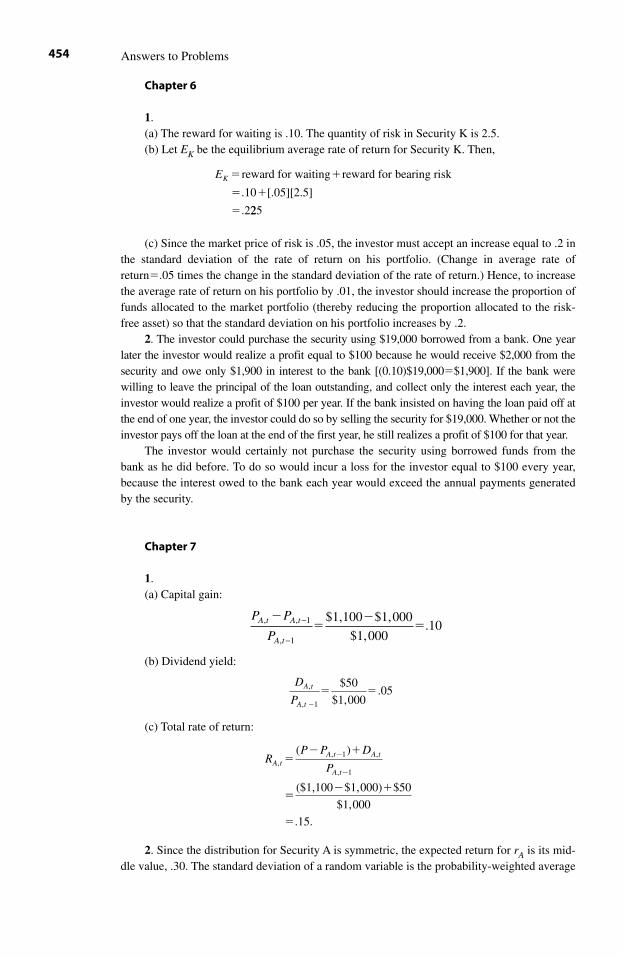
Chapter 6

1.(a) The reward for waiting is .10. The quantity of risk in Security K is 2.5.(b) Let EK be the equilibrium average rate of return for Security K. Then,

(c) Since the market price of risk is .05, the investor must accept an increase equal to .2 inthe standard deviation of the rate of return on his portfolio. (Change in average rate ofreturn�.05 times the change in the standard deviation of the rate of return.) Hence, to increasethe average rate of return on his portfolio by .01, the investor should increase the proportion offunds allocated to the market portfolio (thereby reducing the proportion allocated to the risk-free asset) so that the standard deviation on his portfolio increases by .2.

2. The investor could purchase the security using $19,000 borrowed from a bank. One yearlater the investor would realize a profit equal to $100 because he would receive $2,000 from thesecurity and owe only $1,900 in interest to the bank [(0.10)$19,000�$1,900]. If the bank werewilling to leave the principal of the loan outstanding, and collect only the interest each year, theinvestor would realize a profit of $100 per year. If the bank insisted on having the loan paid off atthe end of one year, the investor could do so by selling the security for $19,000. Whether or not theinvestor pays off the loan at the end of the first year, he still realizes a profit of $100 for that year.

The investor would certainly not purchase the security using borrowed funds from thebank as he did before. To do so would incur a loss for the investor equal to $100 every year,because the interest owed to the bank each year would exceed the annual payments generatedby the security.

Chapter 7

1.(a) Capital gain:

(b) Dividend yield:

(c) Total rate of return:

2. Since the distribution for Security A is symmetric, the expected return for rA is its mid-dle value, .30. The standard deviation of a random variable is the probability-weighted average

RP P D

PA tA t A t

A t,

, 1 ,

, 1

( )

($1,100 $1,000) $50

$1,000

.15.

��

��

�

-

-

D

PA t

A t

,

, 1

$50

$1,000.05

�

� �

P P

PA t A t

A t

, , 1

, 1

$1,100 $1,000

$1,000.10

��

��

−

−

EK � �

� �

�

reward for waiting reward for bearing risk

.10 [.05][2.5]

.2225


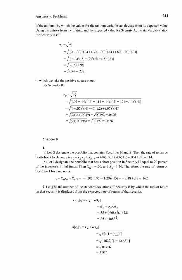
of the amounts by which the values for the random variable can deviate from its expected value.Using the entries from the matrix, and the expected value for Security A, the standard deviationfor Security A is:

in which we take the positive square roots.For Security B:

Chapter 8

1.(a) Let G designate the portfolio that contains Securities H and B. Then the rate of return on

Portfolio G for January is rG�XH rH�XB rB�(.60)(.09)�(.40)(.15)�.054�.06�.114.(b) Let J designate the portfolio that has a short position in Security H equal to 20 percent

of the investor’s initial funds. Then XH��.20, and XB�1.20. Therefore, the rate of return onPortfolio J for January is:

2. Let δ be the number of the standard deviations of Security B by which the rate of returnon that security is displaced from the expected rate of return of that security.

� ��

� �

� �

�

[ ]

[(1 ( ) ]

(.1622) [1 (.668) ]

.0145

2 2

2 2

� �r r EA B B B

A AB

⏐

ρ

66

.1207.�

r X r X rJ H H B B� � � � � � � � �(.20) (.09) (1.20) (.15) .018 .18 .162.

�

� � � � � �

� �

B B2

2 2 2[(.07 .14) (.4) (.14 .14) (.2) (.21 .14) (.4)]

[( .007) (.4) (0) (.2) (.07) (.4)]

(2)(.4)(.0049) 00392 .0626

2 2 2� �

� � �

� ((2)(.00196) 00392 .0626.� �

�

� � � � � �

� �

A A2

2 2 2[(0 .30) (.3) (.30 .30) (.4) (.60 .30) (.3)]

[( .3)22 2 2(.3) (0) (.4) (.3) (.3)]

[2(.3)(.09)]

.054 .232,

� �

�

� �


ˆ( )

ˆ

ˆ.35 (.668) (.1622)ˆ.35 .1083 .

A B B B

A AB A

E r r E

E

� �

� �

� �

� �

δ

δ

δ

δ

� �⏐ s

r s

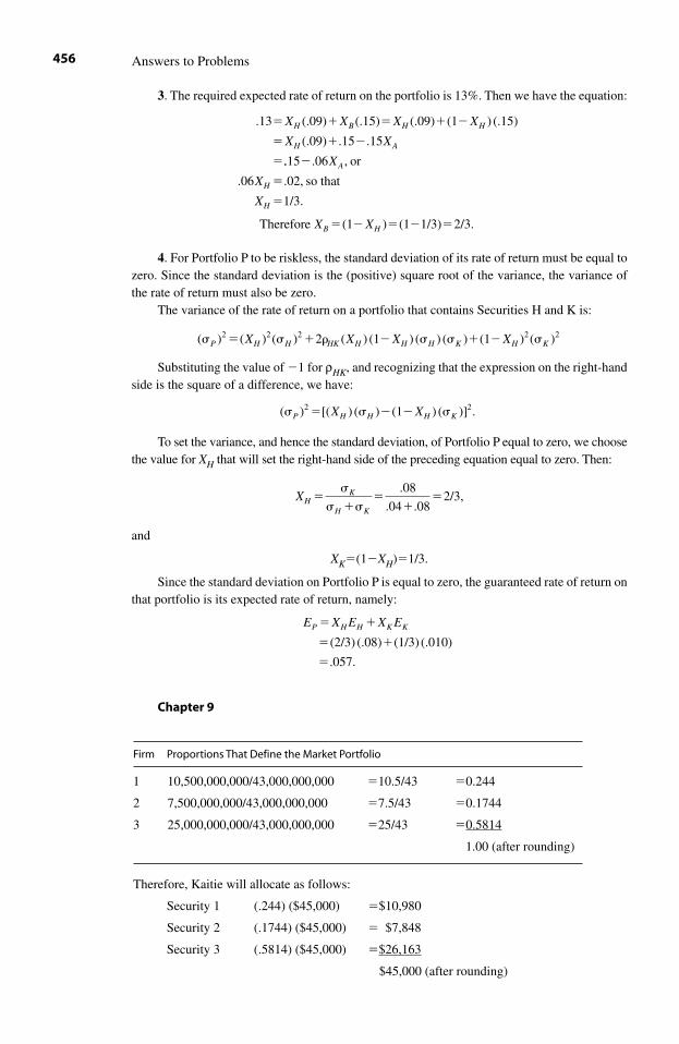
3. The required expected rate of return on the portfolio is 13%. Then we have the equation:

4. For Portfolio P to be riskless, the standard deviation of its rate of return must be equal tozero. Since the standard deviation is the (positive) square root of the variance, the variance ofthe rate of return must also be zero.

The variance of the rate of return on a portfolio that contains Securities H and K is:

Substituting the value of �1 for ρHK, and recognizing that the expression on the right-handside is the square of a difference, we have:

To set the variance, and hence the standard deviation, of Portfolio P equal to zero, we choosethe value for XH that will set the right-hand side of the preceding equation equal to zero. Then:

and

XK�(1�XH)�1/3.

Since the standard deviation on Portfolio P is equal to zero, the guaranteed rate of return onthat portfolio is its expected rate of return, namely:

Chapter 9

E X E X EP H H K K� �

� �

�

(2/3) (.08) (1/3) (.010)

.057.

XHK

H K

�

� �

��

.08

.04 .082/3,

( ) [( ) ( ) (1 ) ( )]2 2 � � � P H H H KX X .

( ) ( ) ( ) 2 ( ) (1 ) ( ) ( ) (1 ) ( )2 2 2 2 2 � � � � � � P H H HK H H H K H KX X X X

Therefore (1 ) (1 1/3) 2/3.X XB H� � � � �

.13 (.09) (.15) (.09) (1 ) (.15)

(.09) .15 .15

� � � � �

� � �

�

X X X X

X XH B H H

H A

..15 .06 , or

.06 .02, so that

1/3.

�

�

�

X

X

X

A

H

H


Firm Proportions That Define the Market Portfolio

1 10,500,000,000/43,000,000,000 �10.5/43 �0.244

2 7,500,000,000/43,000,000,000 �7.5/43 �0.1744

3 25,000,000,000/43,000,000,000 �25/43 �0.5814

1.00 (after rounding)

Therefore, Kaitie will allocate as follows:

Security 1 (.244) ($45,000) �$10,980

Security 2 (.1744) ($45,000) � $7,848

Security 3 (.5814) ($45,000) �$26,163

$45,000 (after rounding)

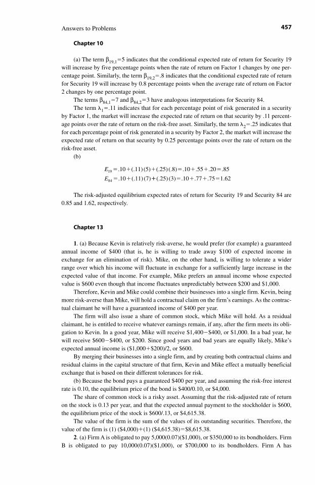
Chapter 10

(a) The term β19,1�5 indicates that the conditional expected rate of return for Security 19will increase by five percentage points when the rate of return on Factor 1 changes by one per-centage point. Similarly, the term β19,2�.8 indicates that the conditional expected rate of returnfor Security 19 will increase by 0.8 percentage points when the average rate of return on Factor2 changes by one percentage point.

The terms β84,1�7 and β84,2�3 have analogous interpretations for Security 84.The term �1�.11 indicates that for each percentage point of risk generated in a security

by Factor 1, the market will increase the expected rate of return on that security by .11 percent-age points over the rate of return on the risk-free asset. Similarly, the term �2�.25 indicates thatfor each percentage point of risk generated in a security by Factor 2, the market will increase theexpected rate of return on that security by 0.25 percentage points over the rate of return on therisk-free asset.

(b)

The risk-adjusted equilibrium expected rates of return for Security 19 and Security 84 are0.85 and 1.62, respectively.

Chapter 13

1. (a) Because Kevin is relatively risk-averse, he would prefer (for example) a guaranteedannual income of $400 (that is, he is willing to trade away $100 of expected income inexchange for an elimination of risk). Mike, on the other hand, is willing to tolerate a widerrange over which his income will fluctuate in exchange for a sufficiently large increase in theexpected value of that income. For example, Mike prefers an annual income whose expectedvalue is $600 even though that income fluctuates unpredictably between $200 and $1,000.

Therefore, Kevin and Mike could combine their businesses into a single firm. Kevin, beingmore risk-averse than Mike, will hold a contractual claim on the firm’s earnings. As the contrac-tual claimant he will have a guaranteed income of $400 per year.

The firm will also issue a share of common stock, which Mike will hold. As a residualclaimant, he is entitled to receive whatever earnings remain, if any, after the firm meets its obli-gation to Kevin. In a good year, Mike will receive $1,400�$400, or $1,000. In a bad year, hewill receive $600�$400, or $200. Since good years and bad years are equally likely, Mike’sexpected annual income is ($1,000�$200)/2, or $600.

By merging their businesses into a single firm, and by creating both contractual claims andresidual claims in the capital structure of that firm, Kevin and Mike effect a mutually beneficialexchange that is based on their different tolerances for risk.

(b) Because the bond pays a guaranteed $400 per year, and assuming the risk-free interestrate is 0.10, the equilibrium price of the bond is $400/0.10, or $4,000.

The share of common stock is a risky asset. Assuming that the risk-adjusted rate of returnon the stock is 0.13 per year, and that the expected annual payment to the stockholder is $600,the equilibrium price of the stock is $600/.13, or $4,615.38.

The value of the firm is the sum of the values of its outstanding securities. Therefore, thevalue of the firm is (1) ($4,000)�(1) ($4,615.38)�$8,615.38.

2. (a) Firm A is obligated to pay 5,000(0.07)($1,000), or $350,000 to its bondholders. FirmB is obligated to pay 10,000(0.07)($1,000), or $700,000 to its bondholders. Firm A has

E

E19

84

.10 (.11) (5) (.25) (.8) .10 .55 .20 .85

.10 (.11) (7)

� � � � � � �

� � �� (.25) (3) .10 .77 .75 1.62


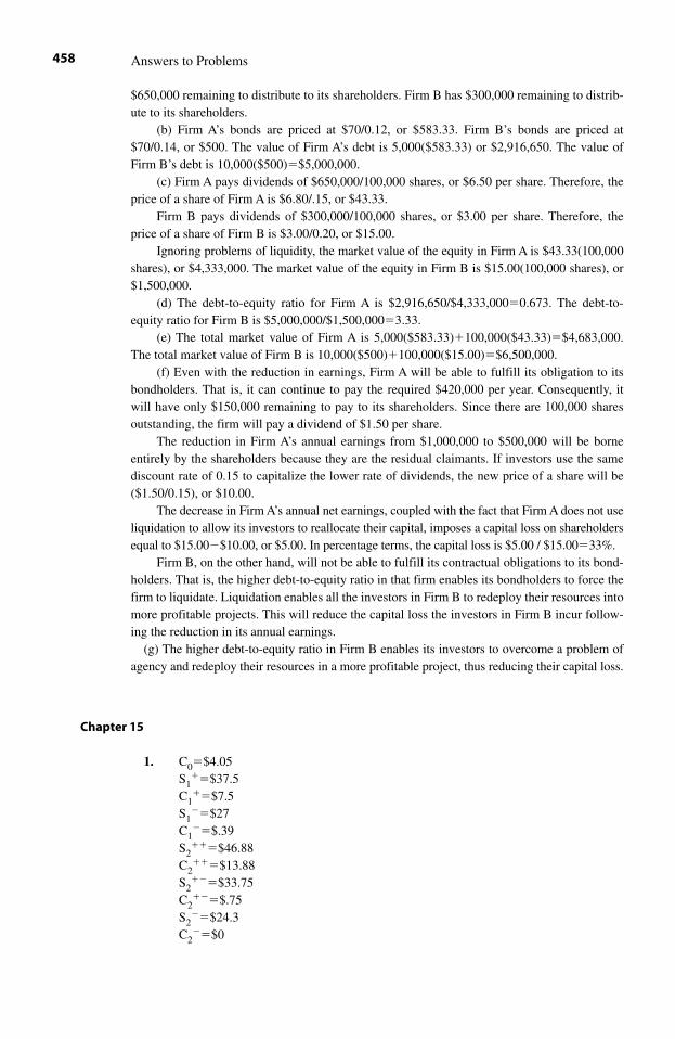
$650,000 remaining to distribute to its shareholders. Firm B has $300,000 remaining to distrib-ute to its shareholders.

(b) Firm A’s bonds are priced at $70/0.12, or $583.33. Firm B’s bonds are priced at$70/0.14, or $500. The value of Firm A’s debt is 5,000($583.33) or $2,916,650. The value ofFirm B’s debt is 10,000($500)�$5,000,000.

(c) Firm A pays dividends of $650,000/100,000 shares, or $6.50 per share. Therefore, theprice of a share of Firm A is $6.80/.15, or $43.33.

Firm B pays dividends of $300,000/100,000 shares, or $3.00 per share. Therefore, theprice of a share of Firm B is $3.00/0.20, or $15.00.

Ignoring problems of liquidity, the market value of the equity in Firm A is $43.33(100,000shares), or $4,333,000. The market value of the equity in Firm B is $15.00(100,000 shares), or$1,500,000.

(d) The debt-to-equity ratio for Firm A is $2,916,650/$4,333,000�0.673. The debt-to-equity ratio for Firm B is $5,000,000/$1,500,000�3.33.

(e) The total market value of Firm A is 5,000($583.33)�100,000($43.33)�$4,683,000.The total market value of Firm B is 10,000($500)�100,000($15.00)�$6,500,000.

(f) Even with the reduction in earnings, Firm A will be able to fulfill its obligation to itsbondholders. That is, it can continue to pay the required $420,000 per year. Consequently, itwill have only $150,000 remaining to pay to its shareholders. Since there are 100,000 sharesoutstanding, the firm will pay a dividend of $1.50 per share.

The reduction in Firm A’s annual earnings from $1,000,000 to $500,000 will be borneentirely by the shareholders because they are the residual claimants. If investors use the samediscount rate of 0.15 to capitalize the lower rate of dividends, the new price of a share will be($1.50/0.15), or $10.00.

The decrease in Firm A’s annual net earnings, coupled with the fact that Firm A does not useliquidation to allow its investors to reallocate their capital, imposes a capital loss on shareholdersequal to $15.00�$10.00, or $5.00. In percentage terms, the capital loss is $5.00 / $15.00�33%.

Firm B, on the other hand, will not be able to fulfill its contractual obligations to its bond-holders. That is, the higher debt-to-equity ratio in that firm enables its bondholders to force thefirm to liquidate. Liquidation enables all the investors in Firm B to redeploy their resources intomore profitable projects. This will reduce the capital loss the investors in Firm B incur follow-ing the reduction in its annual earnings.

(g) The higher debt-to-equity ratio in Firm B enables its investors to overcome a problem ofagency and redeploy their resources in a more profitable project, thus reducing their capital loss.

Chapter 15

1. C0�$4.05S1

��$37.5C1

��$7.5S1

��$27C1

��$.39S2

��$46.88C2

��$13.88S2

��$33.75C2

��$.75S2

��$24.3C2

��$0


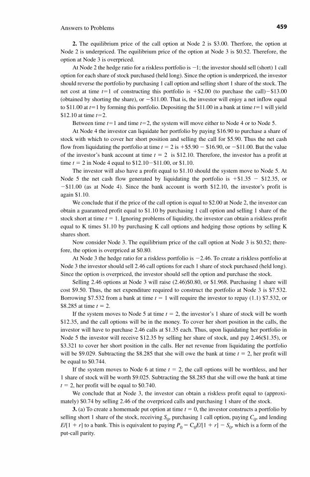
2. The equilibrium price of the call option at Node 2 is $3.00. Therfore, the option at Node 2 is underpriced. The equilibrium price of the option at Node 3 is $0.52. Therefore, theoption at Node 3 is overpriced.

At Node 2 the hedge ratio for a riskless portfolio is �1; the investor should sell (short) 1 calloption for each share of stock purchased (held long). Since the option is underpriced, the investorshould reverse the portfolio by purchasing 1 call option and selling short 1 share of the stock. Thenet cost at time t�1 of constructing this portfolio is �$2.00 (to purchase the call)�$13.00(obtained by shorting the share), or �$11.00. That is, the investor will enjoy a net inflow equalto $11.00 at t�1 by forming this portfolio. Depositing the $11.00 in a bank at time t�1 will yield$12.10 at time t�2.

Between time t�1 and time t�2, the system will move either to Node 4 or to Node 5.At Node 4 the investor can liquidate her portfolio by paying $16.90 to purchase a share of

stock with which to cover her short position and selling the call for $5.90. Thus the net cashflow from liquidating the portfolio at time t � 2 is �$5.90 � $16.90, or �$11.00. But the valueof the investor’s bank account at time t � 2 is $12.10. Therefore, the investor has a profit attime t � 2 in Node 4 equal to $12.10�$11.00, or $1.10.

The investor will also have a profit equal to $1.10 should the system move to Node 5. AtNode 5 the net cash flow generated by liquidating the portfolio is �$1.35 � $12.35, or�$11.00 (as at Node 4). Since the bank account is worth $12.10, the investor’s profit is again $1.10.

We conclude that if the price of the call option is equal to $2.00 at Node 2, the investor canobtain a guaranteed profit equal to $1.10 by purchasing 1 call option and selling 1 share of thestock short at time t � 1. Ignoring problems of liquidity, the investor can obtain a riskless profitequal to K times $1.10 by purchasing K call options and hedging those options by selling Kshares short.

Now consider Node 3. The equilibrium price of the call option at Node 3 is $0.52; there-fore, the option is overpriced at $0.80.

At Node 3 the hedge ratio for a riskless portfolio is �2.46. To create a riskless portfolio atNode 3 the investor should sell 2.46 call options for each 1 share of stock purchased (held long).Since the option is overpriced, the investor should sell the option and purchase the stock.

Selling 2.46 options at Node 3 will raise (2.46)$0.80, or $1.968. Purchasing 1 share willcost $9.50. Thus, the net expenditure required to construct the portfolio at Node 3 is $7.532.Borrowing $7.532 from a bank at time t � 1 will require the investor to repay (1.1) $7.532, or$8.285 at time t � 2.

If the system moves to Node 5 at time t � 2, the investor’s 1 share of stock will be worth$12.35, and the call options will be in the money. To cover her short position in the calls, theinvestor will have to purchase 2.46 calls at $1.35 each. Thus, upon liquidating her portfolio inNode 5 the investor will receive $12.35 by selling her share of stock, and pay 2.46($1.35), or$3.321 to cover her short position in the calls. Her net revenue from liquidating the portfoliowill be $9.029. Subtracting the $8.285 that she will owe the bank at time t � 2, her profit willbe equal to $0.744.

If the system moves to Node 6 at time t � 2, the call options will be worthless, and her 1 share of stock will be worth $9.025. Subtracting the $8.285 that she will owe the bank at timet � 2, her profit will be equal to $0.740.

We conclude that at Node 3, the investor can obtain a riskless profit equal to (approxi-mately) $0.74 by selling 2.46 of the overpriced calls and purchasing 1 share of the stock.

3. (a) To create a homemade put option at time t � 0, the investor constructs a portfolio by selling short 1 share of the stock, receiving S0, purchasing 1 call option, paying C0, and lendingE/[1 � r] to a bank. This is equivalent to paying P0 � C0E/[1 � r] � S0, which is a form of theput-call parity.


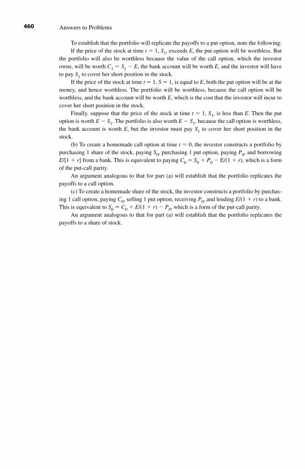
To establish that the portfolio will replicate the payoffs to a put option, note the following:If the price of the stock at time t � 1, S1, exceeds E, the put option will be worthless. But

the portfolio will also be worthless because the value of the call option, which the investorowns, will be worth C1 � S1 � E, the bank account will be worth E, and the investor will haveto pay S1 to cover her short position in the stock.

If the price of the stock at time t � 1, S � 1, is equal to E, both the put option will be at themoney, and hence worthless. The portfolio will be worthless, because the call option will beworthless, and the bank account will be worth E, which is the cost that the investor will incur tocover her short position in the stock.

Finally, suppose that the price of the stock at time t � 1, S1, is less than E. Then the putoption is worth E � S1. The portfolio is also worth E � S1, because the call option is worthless,the bank account is worth E, but the investor must pay S1 to cover her short position in thestock.

(b) To create a homemade call option at time t � 0, the investor constructs a portfolio bypurchasing 1 share of the stock, paying S0, purchasing 1 put option, paying P0, and borrowingE/[1 � r] from a bank. This is equivalent to paying C0 � S0 � P0 � E/(1 � r), which is a formof the put-call parity.

An argument analogous to that for part (a) will establish that the portfolio replicates thepayoffs to a call option.

(c) To create a homemade share of the stock, the investor constructs a portfolio by purchas-ing 1 call option, paying C0, selling 1 put option, receiving P0, and lending E/(1 � r) to a bank.This is equivalent to S0 � C0 � E/(1 � r) � P0, which is a form of the put-call parity.

An argument analogous to that for part (a) will establish that the portfolio replicates thepayoffs to a share of stock.


Agency Problem By administering the enterprise so as to favor its own interestsrather than those of its principal, the agent might exploit the flexibilityprovided by the principal. In a corporation, the principal is the groupof shareholders; the agent is the team of managers employed bythe shareholders to operate the firm. The presence of agency problemscreates economic inefficiencies (deadweight losses) in the allocationof resources.

Arbitrage Pricing Theory (APT) A multifactor model in which theinvestigator uses a mathematical technique called factor analysis to choosethe factors (portfolios) of an asset pricing model. The technique chooses the fac-tors to maximize the accuracy with which the model can explain the expectedrates of return on individual securities by using the sensitivities of the securities’rates of return to the rates of return on the factors. These sensitivities are thesecurities’ quantities of risk with respect to the factors.

Asset Substitution The substitution by a firm of a riskier project for a lessrisky one as a means of transferring wealth from the contractual claimants (e.g., bondholders) to the shareholders, who are the residual claimants.

Asymmetric Information Information that is not available equally to allparties of an exchange. If the parties to a proposed exchange have asymmetricinformation, the parties with the superior information have an incentive to enterthe exchange only in circumstances that are likely to transfer wealth tothemselves from the parties with the inferior information. Being awareof this possibility, the latter parties might refuse to enter the exchange eventhough the exchange, properly structured, could be mutually beneficial.The presence of asymmetric information, unless mitigated, can thus createdeadweight losses.

At the Money An option on an underlying security is “at the money” when thestrike price of the option is equal to the market price of the stock.

Beta A numerical measure of the sensitivity of the expected rate of return on aspecific stock to changes in the rate of return on the market portfolio.Graphically, the value of beta for a security is the slope of that security’scharacteristic line.

Glossary

461

Bond A saleable debt security (contractual claim) issued by a corporation orgovernment guaranteeing to the holder a finite number of interest payments for aspecified period of time, plus a final payment equal to the face value of the bondwhen the bond matures.

Book-to-Market Value of a Firm The ratio of a firm’s book value to its marketvalue. The average book-to-market value of a portfolio of firms is often usedas one of the factors in a multifactor asset pricing model, such as the modelsof Fama and French.

Book Value The estimated amount of money that a firm could raise by sellingall of its assets. Sometimes the book value of a firm is known as the firm’sliquidation value, or its salvage value. The book value usually includes a termcalled “good will,” which is an estimate of the value that the firm’s managementcontributes to the ability of the firm to generate earnings. Due to thedifficulty of separating the contributions of the firm’s saleable assets and thefirm’s management to the firm’s ability to generate earnings, the “good will”is entered as an arbitrary figure, such as $1,000,000, or even $1.

Callable Bond A bond that the issuing firm has the right to cancel by paying tothe bond’s current owners a fixed price (the call price) that is specified in thedefinition of that bond.

Call Option A contract that gives the holder the right (but not the obligation)to buy a given security at a fixed price within a specified period of time.

Call Price of a Bond The amount of money a firm must pay to bondholders inorder to cancel a callable bond.

Capital Asset Pricing Model (CAPM) A model that defines the relationshipin equilibrium between the expected rate of return on a security and thequantity of systematic risk contained in that security. The graphicalrepresentation of this relationship is the Security Market Line.

The central idea of the CAPM is that in equilibrium each investor willadjust the levels of expected return and standard deviation on her portfolioby choosing the proportion in which to split her funds between a risk-freegovernment bond and a unique efficient portfolio that contains the riskysecurities of every firm in the economy. This unique efficient portfoliois called the market portfolio. Within the market portfolio, the proportionof funds allocated to each firm is equal to the ratio of the market value ofthat firm’s securities to the aggregate market value of all firms’ securities.

Capital Gain The amount by which the current market price of an asset exceedsthe original cost of that asset.

Capitalized Value (of a sequence of payments) The net present value of thesequence. The capitalized value of a firm is the total market value of thefirm’s common stock. Since the price of a share is the (risk-adjusted)net present value of the firm’s earnings per share (as perceived by investors),the capitalized value of a firm is the (risk-adjusted) net present value of the firm’sresidual earnings.

Glossary462

Capital Market Line The line in the CAPM that defines the tradeoff inequilibrium between expected rate of return and standard deviation forefficient portfolios. The Capital Market Line extends from the risk-free rateof return on the vertical axis to a point of tangency on the concave locusof efficient combinations of expected rate of return and standard deviationfor portfolios that contain only risky assets. This point of tangency definesthe market portfolio.

Capital Structure The configuration of claims on the firm’s earnings held byinvestors. These claims are partitioned into contractual claims (e.g., bonds)and residual claims (e.g., common stock). The capital structure of a firmcan affect economic efficiency by mitigating or exacerbating problemsof agency and asymmetric information.

Characteristic Line Each security has its own characteristic line that defines theconditional expected return on that security for period t as a linear function ofthe rate of return on the market portfolio for period t. The slope of a security’scharacteristic line is the value of beta for that security.

Comparative Advantage The amount by which the cost incurred by oneperson (or firm) to produce some Good X is less than the cost incurredby a second person (or firm) to produce that same Good X. For each person,the cost of producing Good X is measured in terms of the quantity of someGood Y foregone. That is, the cost of producing Good X is the real cost,as measured in terms of Good Y foregone.

Concavity A measure of the curvature of line for which the chord betweenany two points on the line lies below the line.

Conditional Expected Rate of Return The expected rate of return(on a security) when the value of some other variable (such as the rateof return on the market portfolio) is pre-specified.

Conditional Probability Density Function The probability density functionof a random variable (such as the rate of return on a security) when the valueof some other variable (such as the rate of return on the market portfolio)is pre-specified.

Conversion Ratio The fixed number of shares of a firm’s stock that the holderof a convertible bond issued by that firm receives by surrendering the bond andpaying a fixed price specified in the convertible bond.

Convertible Bond A bond that gives the bond’s owner an option to convert thebond into a fixed number of shares of the firm’s common stock at a fixed price.

Convexity A measure of the curvature of line for which the chord between anytwo points on the line lies above the line.

Correlation Coefficient (“closeness of fit”) An index of the average proximityof a set of data points to their regression line. If all the data points lieon the regression line, the correlation coefficient is equal to �1 if the line has apositive slope, and �1, if the line has a negative slope.

Glossary 463

Coupon Rate of a Bond The percentage of the face value of a bond that the issu-ing firm must pay periodically to the investor who holds the bond.The coupon rate of a bond is the rate of return on the bond if and only ifthe market price of the bond is equal to the face value of that bond.

Covariance The covariance between any two random variables is theprobability-weighted sum of the products of the amounts by whichthe value of each random variable can deviate from its expected value.

Dead Weight Loss The value of potential mutually beneficial exchangesforegone as a consequence of an inefficient allocation of resources.

Debt A contractual claim on a firm’s earnings. Also, the totality of the contractualclaims on a firm’s earnings.

Debt/Equity Ratio Also known as leverage. The ratio of the market valueof firm’s debt securities (contractual claims) to the market value of a firm’sequity securities (residual claims).

Economic Efficiency An evaluation of an allocation of resources in termsof mutually beneficial exchanges. An allocation is economically efficientif there exist no alternative allocations that would provide at least one personwith a gain in utility (or wealth), without imposing a loss on any person.Equivalently, an allocation is economically efficient if there are no furtheropportunities for mutually beneficial exchanges, that is, if there are nodeadweight losses.

Economic Equivalence Two sequences of payments are economically equiva-lent if they have the same present value. Consequently, an investor who can bor-row from and lend to a bank can convert any sequence of payments to any othersequence that is economically equivalent to the first sequence.

Economic Rent That portion of the income received by the owner of a resourcethat exceeds the owner’s opportunity cost. Hence, if the owner of a resourcewere to incur a fixed cost (i.e., a cost that does not depend on the rate of output)that does not exceed her economic rent, she would continue to produce the samerate of output that she did before the cost was incurred. (A change in a marginalcost would induce a change in the owner’s choice of the quantity of output toproduce.) Economic rent is synonymous with economic profit and producer’ssurplus.

Efficient Allocation of Resources See Economic Efficiency

Efficient Markets Hypothesis The assertion that the current prices of securitiesreflect all information that is currently known about the future payments that theowners of the securities will receive. An implication of the Efficient MarketsHypothesis is that the net marginal benefit of searching for mispriced securitiesor attempting to predict movements in the general level of prices of securities(i.e., “time the market”) is equal to zero.

The prices of securities reflect the willingness of investors to buy, sell, andhold positions in those securities. Therefore, if the prices are to reflect

Glossary464

information, there must be some investors whose trading causes the pricesto change when information changes. For these investors, the net marginalbenefit of searching for mispriced securities must be positive, else theseinvestors would have no incentive to search for information. Consequently,the Efficient Markets Hypothesis cannot be true for every investor; if theEfficient Markets Hypothesis is true, there must be some investors who havea comparative advantage in analyzing information about the prices of securities.

Equilibrium A configuration of prices and quantities for which the quantitysupplied of each good is equal to the quantity demanded. The goods can includefinancial securities.

Equity A residual claim on a firm’s earnings. Also, the totality of the residualclaims on the firm’s earnings

Exercise (Strike) Price The fixed price at which the owner of a call (put) optioncan buy (sell) the underlying security at any time before the option expires.

Expected Rate of Return The expected value of the rate of return on a security.See also Expected Value.

Expected Value The sum of the values that a random variable can take, with eachvalue weighted by the probability that the variable can take that value.

Face Value (of a Bond) The amount of money that the issuer of the bond mustpay to the holder of the bond on the maturity date of that bond. The face value ofa bond is specified by the contract that defines the bond. The price of a bond isnot necessarily equal to the bond’s face value; as is the case for any financialsecurity, the price of a bond is set by the willingness of investors to hold thatbond in their portfolios.

Financial Asset A claim on the earnings of a real asset. Sometimes usedinterchangeably with “financial security.”

Financial Security A saleable right to receive a sequence of payments over time.The payments can continue for a finite number of periods (as in a bond) or foran indefinite number of periods (as in a share of stock). The size of thepayments can be specified in advance (as in a bond) or be determinedby a probability density function (as in a share of stock).

Homemade Dividend A payment that a shareholder can create, for each share thatshe owns, by selling a portion of that share. The concept of a homemade dividend ismost commonly used to illustrate how a shareholder can obtain the net presentvalue per share of a new investment project that the firm finances by retainedearnings. If a firm finances a project by retaining earnings that it would otherwisehave paid to its shareholders as dividends, the increase in the price of a share willbe equal to the sum of the net present value of the project per share plus the amountby which the current dividend decreases. [The preceding statement holds withoutqualification if there is no uncertainty about future events. When there is uncer-tainty about future events (such as the outcomes of a new investment project), thepreceding statement must be qualified.]

Glossary 465

Idiosyncratic (Firm-Specific) Risk A measure of the amount by which a firm’searnings are affected by factors other than the level of macroeconomic activity,such as the prices that it pays for inputs, the strength of the demand for itsproducts, litigation, resignations of critical executives, and the actions ofregulatory authorities. In the CAPM, the variance of the vertical distancesbetween the data points for a security and the characteristic line for thatsecurity is the idiosyncratic risk of that security.

Imbedded Option Synonymous with an implicit option.

Implicit Option An opportunity to postpone for a fixed amount of time adecision to acquire at a fixed price an asset other than a financial security.The option is implicit because the underlying asset is not traded on anorganized exchange. Consequently, the use of the Black-Scholes option pricingmodel is not as transparent as in the case of a conventional option, such as a calloption or a put option. By contrast, a conventional option is explicit because theunderlying asset is traded on an organized exchange.

An example of an implicit option is the opportunity of a firm to postpone adecision to undertake an investment project in order to collect additionalinformation about the future outcomes of the project. The option to postpone thedecision has a value, which can be analyzed by using versions of theBlack-Scholes model. Recognizing implicit options enables one to include in thecalculation of the opportunity cost of a project the value foregone bybeginning the project now rather than postponing the project in order to collectadditional information.

A second example of an implicit option arises in the case of a leveragedfirm. Rather than regard the shareholders as the owners of the firm, we canregard the firm’s bondholders as owning the firm and as giving shareholdersan option to acquire the firm by making the contractual payments of interest andface value to the bondholders. Viewed in this way, the shareholders havean option to postpone a decision to pay the bondholders until the shareholderslearn whether the firm will be profitable in future periods. The exercise priceof the implicit option is the set of promised payments of interest and face value.If the firm will be profitable, the shareholders will “exercise” their optionto acquire the firm by causing the firm to pay the bondholders. If the firm willnot be profitable, the shareholders will allow their option to expire unexercisedby causing the firm to default on the bonds.

Information Trading Trading by investors who believe that the current price of asecurity does not correctly reflect the risk-adjusted net present value of thesequence of payments associated with that security. Distinguished fromliquidity trading.

Internal Rate of Return (of a sequence of payments) The discount ratefor which the net present value of the sequence of payments is equal to zero.Consequently, the internal rate of return of a sequence is the maximal rateof interest that an investor could afford to pay on funds borrowed to finance thepurchase of the sequence, assuming that the investor could earn interest at that

Glossary466

same rate by depositing in the bank the payments generated by that sequence.See also Yield-to-Maturity (of a bond).

In the Money An option is “in the money” if an immediate exercise of theoption would create a gross profit for the owner of that option, excluding anyconsideration of the price that the owner paid to acquire the option. A call optionis in the money if the current price of the stock exceeds the exercise price speci-fied by the option. A put option is in the money if the currentprice of the stock is less than the exercise price specified by the option.

Joint Hypothesis If investors could outperform the market by using a particularstrategy, there are always two competing explanations between which theeconomist can not distinguish. One explanation is that the Efficient MarketsHypothesis does not hold; there is information about future earnings thatis not accurately reflected in current prices. The competing explanation is thatthe economist is using the wrong model to define the equilibrium relationshipbetween expected rates of return, waiting, and risk.

Similarly, if there is evidence that investors cannot outperform the market,either the Efficient Markets Hypothesis holds, or economists are using thewrong model to define the equilibrium tradeoff between expected rate of returnand risk.

Lambda The market price of risk associated with a specific factor in a multifactorasset pricing model. A multifactor asset pricing model has as many marketprices of risk as the model has factors.

Leverage The ratio of the total market value of a firm’s debt securities to the totalmarket value of its equity securities. Also known as the firm’s debt/equity (ord/e) ratio.

Liquidity A measure of the increase in the cost that one would incur as aconsequence of increasing either the size of a transaction in that asset orthe speed at which the investor wants to conclude the transaction.

Liquidity Trading Trading by investors to adjust either the size or the level ofrisk in their portfolios. Distinguished from information trading.

Long Position A long position in an asset is a position in which the investorwill lose wealth if the price of the asset falls and gain wealth if the price of theasset rises.

Market Portfolio A portfolio consisting of every risky security in the economy.The proportion in which a particular security appears in the market portfoliois equal to the proportion of the total value of the outstanding shares of thatsecurity relative to the sum of the total values of the outstanding shares of all therisky securities in the economy. The market portfolio is an essential feature ofthe CAPM.

Market Price of Risk The increase in the average rate of return on anefficient portfolio that an investor can obtain if she accepts an increaseof one percentage point in the standard deviation of the rate of return on that

Glossary 467

portfolio. Therefore, the market price of risk is the rate at which the marketcompensates an investor for bearing risk.

Market Value of a Firm The total market value of the firm’s securities. Ignoringconsiderations of liquidity, the market value of a firm is the amount of moneythat investors would have to pay to purchase the totality of the claims on thefirm’s earnings (and thereby purchase the firm itself).

Maturity Date (of a bond) The date on which the issuer of the bond must pay tothe holder of the bond the face value of the bond. On the maturity date theperiodic payments of interest cease.

Multifactor (Asset-Pricing) Model An alternative to the CAPM in which thereis more than one source of systematic risk. In a multifactor model theequilibrium expected rate of return on a security is equal to a reward for waitingplus a sum of terms to adjust for risk. Each adjustment for risk is a product oftwo terms. One of these terms is the quantity of a particular type of systematicrisk; the other term is the market price for that type of risk. The quantity of riskcontained in a security relative to a given factor is the beta of that security forthat factor. The market price of risk for a factor is the lambda for that factor.

Net Present Value (of a sequence of payments) The amount of money that,if deposited in a bank today, would enable the depositor to make a sequence ofwithdrawals that would exactly replicate the timing and the sizes of thepayments in the sequence.

Out of the Money An option is “out of the money” if an immediate exercise ofthe option would create a gross loss for the owner of that option, excluding anyconsideration of the price that the owner paid to acquire the option. A call optionis out of the money if the current price of the stock is less than theexercise price specified by the option. A put option is out of the money if thecurrent price of the stock exceeds the exercise price specified by the option.

Perfect Negative Correlation If the rates of return on Securities A and B areperfectly negatively correlated, the correlation coefficient between twosecurities is equal to �1. If the rates of return are jointly normally distributed,the values of the two rates of return will always lie on opposite sides of theirrespective expected values by the same number of their respective standarddeviations. For example, suppose that at time t the rate of return on Security A isdisplaced from its expected value in a given direction by a distance equal to z ofits standard deviations. Then at that same time t the rate of return on Security Bwill be displaced from its expected value in the opposite direction by a distanceequal to the same value, z, of its standard deviations.

Perfect Positive Correlation Analogous to perfect negative correlation. Forperfect positive correlation, the correlation coefficient between SecuritiesA and B is equal to +1. The paired deviations of the rates of return on SecuritiesA and B are in the same direction from their expected values.

Portfolio A collection of securities in which the proportions of the total valueof the portfolio allocated to the constituent securities are specified.

Glossary468

Probability Density Function A function that specifies the densities with whicha continuous random variable takes various values. The values of the randomvariable are plotted on the horizontal axis; probability densities are plotted onthe vertical axis. The area under the density function between any two given val-ues for the random variable is the probability that the random variable will takea value between the given values. By definition of probability, the total areaunder the density function is equal to 1.0. A normal density function is a bell-shaped curve that is symmetrical around the expected value of the random vari-able.

Probability Distribution A list of the probabilities with which a random variablewill take its possible values.

Put Option A contract that gives the holder the right (but not the obligation) tosell a given security at a specific price within a specific time period.

Quantity of Risk The quantity of systematic risk contained in a security isproportional to the sensitivity of the rate of return on that security to variationsin the rate of return on the market portfolio. The market portfolio is a proxy forthe level of macroeconomic activity. In the CAPM the quantity of systematicrisk in a security is the value of the beta for that security.

Real Asset A factor of production that can generate earnings by producing avaluable good or service.

Real Option An option to purchase or sell a real asset.

Regression Line A straight line whose slope and vertical intercept summarize therelationship between paired values for two variables. In the CAPM, the characteristic line for a security is the line obtained by regressing the rate ofreturn on that security (plotted on the vertical axis) against the rate ofreturn on the market portfolio (plotted on the horizontal axis).

Risk-Adjusted Residual The vertical distance between the rate of return on asecurity and the characteristic line for the security. Equivalently, in the CAPM,that portion of the rate of return at time t that can not be attributed to either thereward for waiting or the reward for bearing risk.

Risk Aversion An investor is risk averse if the average rate of return that she musthave to hold a security increases as the level of unpredictable variability in therate of return on that security increases.

Risk-Free Portfolio A portfolio that has a guaranteed rate of return becausethe proportions in which the constituent securities are held guaranteesthat the random variations of each security’s rate of return will be mutuallyoffsetting.

Risk-Free Rate of Return A rate of return that has a zero probability of deviatingfrom its expected value. A U.S. government bond that has a guaranteed rateof return is regarded as risk-free, because the government has the power to taxand to print money. A corporate bond is not a risk-free asset because the issuingfirm may be unable to make the promised payments.

Glossary 469

Risk Neutrality An investor is risk neutral if she evaluates a security based onlyon its expected rate of return; measures of dispersion (or unpredictablevariability in the rate of return on that security), such as the standard deviationand beta, are irrelevant to the investor.

Security See Financial Security.

Security Market Line A linear relationship that defines the set of alternativecombinations of systematic risk (beta) and expected return for individualsecurities when the market is in equilibrium. The Security Market Line is theessence of the CAPM.

Security Market Plane A plane (or hyperplane) that is analogous for amultifactor model to the Security Market Line for the CAPM. The plane has asmany “horizontal” dimensions as there are factors in the model. For a givensecurity, the values of the betas for each of the factors are plotted in thesehorizontal dimensions. The expected rate of return on the security is measured inthe “vertical” dimension. The value of the lambda for each factor is theslope of the hyperplane in the “horizontal” dimension in which the beta for thatfactor is plotted.

Short Position A short position in an asset is a position in which the investor willgain wealth if the price of the asset falls, and lose wealth if the price of the assetrises.

Short Selling The process of selling a borrowed asset in order to acquire a shortposition.

Standard Deviation The positive square root of the sum of squared deviationsfrom its expected value that the variable can take, with each deviation weightedby the probability that it can occur.

Stock A saleable right to receive an indefinitely long sequence of futurepayments, with the size of each payment contingent on the firm’s futureearnings, on the firm’s future opportunities to identify and finance newinvestment projects, and on the firm’s decisions on what portions of earnings todistribute as dividends. See Homemade Dividend.

Systematic Risk The sensitivity of the rate of return on a security to fluctuationsin the rate of return on the market portfolio.

Transaction Costs A term used to describe any and all costs that individualsincur to make exchanges.

Variance The square of the standard deviation.

Volatility A measure of the magnitude and the rate at which the value of arandom variable can change unpredictably.

Yield-to-Maturity (of a bond) The rate of return that would set the net presentvalue of the sequence of payments generated by the bond equal to thecurrent price of that bond. The yield to maturity on a bond is therefore the

Glossary470

maximal rate of interest that an investor could afford to pay on funds borrowedto finance the purchase of the bond, assuming that the investor could earninterest at that same rate by depositing in the bank the payments generated bythat bond.

Equivalently stated, consider the purchase of a bond as an investmentproject. The expenditure required to initiate the project is the price of the bond,and the periodic payments of interest and the payment of the face value whenthe bond matures are the earnings of the project. Viewed as an investmentproject, the bond has a net present value. The internal rate of return of thebond is the rate of interest for which the net present value of the bond viewed asan investment project would be equal to zero. Consequently, the internal rate ofreturn of a bond is the maximal rate of interest that an investor could afford topay on funds borrowed to purchase the bond.

Zero (coupon bond) A bond on which the coupon rate is equal to zero.Consequently, the issuer of the bond (the borrower) makes no periodicpayments of interest. The issuer does pay the face value of the bond to the bond-holder when the bond matures. The investor (the lender) obtainsinterest implicitly because the price at which the investor purchasesthe bond is less than the face value of the bond.

Glossary 471


What follows is a selected bibliography of the works of Nobel laureates who havecontributed to the economics of financial markets.1

1985 Franco Modigliani

For his pioneering analyses of saving and of financial markets.

Modigliani, Franco (with Merton H. Miller). “The Cost of Capital, Corporation Finance, andthe Theory of Investment.” American Economic Review (June 1958).

1990 Harry M. Markowitz, Merton H. Miller, William F. Sharpe

For their pioneering work in the theory of financial economics.

Markowitz, Harry. “Portfolio Selection.” Journal of Finance (1952).——. “Portfolio Selection: Efficient Diversification of Investment” (1958).——. “Foundations of Portfolio Theory.” Journal of Finance (1991).Miller, Merton (with F. Modigliani). “The Cost of Capital, Corporation Finance and the Theory

of Investment.” American Economic Review (June 1958). ——. “Dividend Policy, Growth and the Valuation of Shares.” Journal of Business (October 1961). Miller, Merton (with E. F. Fama). The Theory of Finance. New York: Holt, Rinehart and

Winston, 1972.Miller, Merton (with Kevin Rock). “Dividend Policy under Asymmetric Information.” Journal

of Finance (September 1985).Miller, Merton. “Financial Innovation: The Last Twenty Years and the Next.” Revue de la

Banque (September 1986). [An expanded version appears in Journal of Financial andQuantitative Analysis 21, no. 4 (December 1986).]

——. “The Modigliani-Miller Propositions after Thirty Years.” Journal of EconomicPerspectives (Fall 1988).

——. “Leverage.” Nobel Prize Lecture, December 7, 1990, Stockholm, Sweden. [Reprinted inJournal of Finance 46, no. 2 (June 1991).]

Bibliography of Nobel Laureates

473

1 NobelPrize.org, Nobel Foundation web group, 1994; available at http://nobelprize.org.

http://nobelprize.org

——. “Index Arbitrage: Villain or Scapegoat?” Journal of Financial Engineering 1, no. 3(December 1992).

Sharpe, William. “Capital Asset Prices—A Theory of Market Equilibrium Under Conditions ofRisk.” Journal of Finance (September 1964): 425–442.

——. “Mutual Fund Performance.” Journal of Business (January 1966): 119–138. ——. Portfolio Theory and Capital Markets. New York: McGraw-Hill, 1970.——. “The Capital Asset Pricing Model: A ‘Multi-Beta’ Interpretation.” Financial Decision

Making Under Uncertainty, Haim Levy and Marshall Sarnat, eds., 127–136. New York:Academic Press 1977.

——. “Capital Asset Prices with and without Negative Holdings.” Nobel Prize Lecture,December 7, 1990, Stockholm, Sweden. [Reprinted in Journal of Finance (June 1991):489–509.]

1997 Robert C. Merton, Myron S. Scholes

For a new method to determine the value of derivatives.

Merton, Robert C. “An Intertemporal Capital Asset Pricing Model.” Econometrica 41(September 1973).

——. “On Market Timing and Investment Performance Part I: An Equilibrium Theory of Valuefor Market Forecasts.” Journal of Business 54 (July 1981).

Merton, Robert C., and R. D. Henriksson. “On Market Timing and Investment PerformancePart II: Statistical Procedures for Evaluating Forecasting Skills.” Journal of Business 54(October 1981).

Merton, Robert C. “Financial Economics.” In Paul Samuelson and Modern Economic Theory,E. C. Brown and R. M. Solow, eds. New York: McGraw-Hill, 1983.

——. “A Simple Model of Capital Market Equilibrium with Incomplete Information.” Journalof Finance 42 (July 1987).

——. “In Honor of Nobel Laureate, Franco Modigliani.” Economic Perspectives 1 (Fall 1987).——. “Applications of Option-Pricing Theory: Twenty-Five Years Later.” American Economic

Review 88, no. 3 (June 1988): 323–349.——. “Capital Market Theory and the Pricing of Financial Securities.” In Handbook of

Monetary Economics, B. Friedman and F. Hahn, eds. Amsterdam: North-Holland (1990).——. Continuous-Time Finance. Oxford, U.K.: Basil Blackwell, 1990. (Rev. ed., 1992.)Merton, Robert C. (with A. Perold). “Theory of Risk Capital in Financial Firms.” Journal of

Applied Corporate Finance (Fall 1993).Scholes, Myron M. (with Fischer Black and Michael Jensen). “The Capital Asset Pricing

Model: Some Empirical Tests.” In Studies in the Theory of Capital Markets, MichaelC. Jensen, ed. New York: Praeger, 1972.

Scholes, Myron M. (with Fischer Black). “The Valuation of Option Contracts and a Test ofMarket Efficiency.” Journal of Finance (1972).

——. “The Pricing of Options and Corporate Liabilities.” JPE (1973).——. “The Effects of Dividend Yield and Dividend Policy on Common Stock Prices and

Returns.” Journal of Financial Economics (1974).Scholes, Myron M. “Taxes and the Pricing of Options.” Journal of Finance (1976).Scholes, Myron M. (with Merton H. Miller). “Dividends and Taxes.” Journal of Financial

Economics (1978).

Bibliography of Nobel Laureates474

2001 George A. Akerlof, A. Michael Spence, Joseph E. Stiglitz

For their analyses of markets with asymmetric information.

Akerlof, George. “The Market for ‘Lemons’: Quality Uncertainty and the Market Mechanism.”Quarterly Journal of Economics (August 1970).

——. An Economic Theorist’s Book of Tales. Cambridge, U.K.: Cambridge University Press,1984.

——. “Gift Exchange and Efficiency Wage Theory: Four Views.” American Economic Review(May 1984).

——. “Introduction.” In Efficiency Wage Theories of the Labor Market, George A. Akerlof and Janet Yellen, eds. Cambridge, U.K.: Cambridge University Press, 1986.

Akerlof, George, and Janet Yellen. “The Fair Wage-Effort Hypothesis and Unemployment.”Quarterly Journal of Economics (May 1990).

Spence, Michael, and Richard Zeckhauser. “Insurance, Information, and Individual Action.”American Economic Review 61, no. 2 (1971): 380–387.

Spence, Michael. “Job Market Signaling.” The Quarterly Jounal of Economics 87, no. 3 (1973):355–374.

——. “Informational Aspects of Market Structure: An Introduction.” The Quarterly Journal ofEconomics 90, no. 4 (1976): 591–597.

——. “Investment, Strategy, and Growth in a New Market.” Bell Journal of Economics (1979).——. “Competition, Entry, and Antitrust Policy, Strategy, Predation, and Antitrust Analysis,”

Federal Trade Commission (September 1981).——. Competitive Structure in Investment Banking. Cambridge, Mass.: Harvard University

Press, 1983.——. “Signaling in Retrospect and the Informational Structure of Markets.” American

Economic Review 92, no. 3 (2002): 434–459.Stiglitz, Joseph. “Modigliani, the Modigliani-Miller Theorem, and Macroeconomics.” Paper

presented to a conference, “Franco Modigliani and the Keynesian Legacy.” New SchoolUniversity, New York, N.Y., April 14–15, 2005.

——. “Information and the Change in the Paradigm in Economics.” The American Economist47 nos. 2 and 3 (Fall 2003 and Spring 2004). Also published in Les Prix Nobel, ToreFrangsmyr, ed., 472–540. Stockholm, Sweden: The Nobel Foundation, 2002; and inRevista Asturiana De Economia 25 (December 2002): 95–164.

——. “The Contributions of the Economics of Information to Twentieth Century Economics.”Quarterly Journal of Economics 115, no. 4 (November 2000): 1441–1478.

Bibliography of Nobel Laureates 475


Akerlof, George A. “The Market for ‘Lemons’: Quality Uncertainty and the MarketMechanism.” Quarterly Journal of Economics (March 1984): 488–500.

Alchian, Armen A., and William R. Allen. Exchange and Production: Competition,Coordination, and Control, 3rd ed. Belmont, Calif.: Wadsworth, 1983.

Alchian, Armen A., and Harold Demsetz. “The Property Rights Paradigm.” Journal ofEconomic History 33 (1973): 16–27.

Arrow, Kenneth J., declaration of, U.S. v. Microsoft, January 17, 1995.Barbour, Brad M., and Terrance Odean. “Trading is Hazardous to Your Wealth: The Common

Stock Investment Performance of Individual Investors.” Journal of Finance 55, no. 2(April 2000): 773–806.

Bittlingmayer, George, and Thomas W. Hazlett. “DOS Kapital: Has Antitrust Action againstMicrosoft Created Value in the Computer Industry?” Journal of Financial Economics,no. 55 (2000): 329–359.

Black, Fischer, and Myron Scholes. “The Pricing of Options and Corporate Liabilities.”Journal of Political Economy 81, no. 3 (1973): 637–659.

Brander, J. A., and T. R. Lewis., “Oligopoly and Financial Structure: The Limited LiabilityEffect.” American Economic Review 76 (1986): 956–970.

Brooks, Robert, Sinclair Davidson, and Robert Faff. “Sudden Changes in Property Rights: TheCase of Australian Native Title.” Journal of Economic Behavior & Organization 52(2003): 427–442.

Chen, N., R. Roll, and S. Ross. “Economic Forces and the Stock Market.” Journal of Business59, no. 3 (1986): 383–403.

Ching W. K., and M. S. Lee. “A Random Walk on a Circular Path.” International Journal ofMathematical Education in Science and Technology 36, no. 6 (2005): 680–683.

deBondt, Werner, and Richard Thaler. “Does the Stock Market Overreact?” In Advances inBehavioral Finance. Edited by Richard H. Thaler. New York: Russell Sage Foundation, 1993.

Demsetz, Harold J. “Toward a Theory of Property Rights.” American Economic Review:Papers and Proceedings (1967): 347–359.

——. “The Cost of Transacting.” Quarterly Journal of Economics 82, no. 1 (1968): 33–53.Duffie, Darrell. Futures Markets. Englewood Cliffs, N.J.: Prentice Hall, 1989.Ellison, Sara Fisher, and Wallace P. Mullin. “Gradual Incorporation of Information:

Pharmaceutical Stocks and the Evolution of President Clinton’s Health Care Reform.” The Journal of Law and Economics 44 (April 2001): 89–130.

Elton, Edwin J., Martin J. Gruber, Stephen J. Brown, and William N. Goetzmann. ModernPortfolio Theory and Investment Analysis, 6th ed. New York: John Wiley & Sons, 2003.

Fama, Eugene F. “Efficient Capital Markets: A Review of Theory and Empirical Work.” The Journal of Finance 25, no. 2 (1970): 383–417.

Bibliography

477

——. “Efficient Capital Markets: II.” Journal of Finance 46, no. 5 (December 1991):1575–1617.

Fama, Eugene F., and Kenneth R. French. “Common Risk Factors in the Returns on Stocks andBonds.” Journal of Financial Economics (February 1993): 3–56.

Fama, Eugene F., and Merton H. Miller. The Theory of Finance. New York: Holt, Rinehart andWinston, 1972.

“The Force of an Idea.” The New Yorker, January 12, 1998.Harris, Larry. Trading and Exchanges: Market Microstructure for Practitioners. New York:

Oxford University Press, 2002.Hilsenrath, Jon E. “Stock Characters: As Two Economists Debate Markets . . . Mr. Thaler Takes

on Mr. Fama.” The Wall Street Journal, Monday, October 18, 2004, A1.Hu, Jie, and Thomas H. Hoe. “The Insider Trading Debate.” Federal Reserve Bank of Atlanta

Economic Review (Fourth Quarter 1997).Hull, John C. Options, Futures, and Other Derivatives, 6th ed. Englewood Cliffs, N.J.: Prentice

Hall, 2006.Jaffe, Jeffrey. “Special Information and Insider Trading.” Journal of Business 47, no. 3 (July

1974): 410.Jensen, Michael C. “Don’t Freeze the Arbs Out.” The Wall Street Journal, December 3, 1986,

editorial page.——. “Risk, the Pricing of Capital Assets, and the Evaluation of Investment Portfolios.”

Journal of Business 42, no. 2 (1969): 167.Jensen, Michael C., and William H. Meckling. “Theory of the Firm: Managerial Behavior,

Agency Costs and Ownership Structure.” Journal of Financial Economics (October 1976):305–360.

Keown, Arthur, and John M. Pinkerton. “Merger Announcements and Insider Trading Activity:An Empirical Investigation.” Journal of Finance 36, no. 4 (September 1981): 855–869.

Landsburg, Steven E. “Random Walks and Stock Prices.” In The Armchair Economist:Economics and Everyday Life, 188–196. New York: The Free Press, 1993.

“The Legend of Arthur.” Slate Magazine, January 14, 1998.Leland, Hayne E. “Insider Trading: Should it be Prohibited?” The Journal of Political

Economy, no. 100 (1992): 859.Lintner, John. “The Valuation of Risk Assets and the Selection of Risky Investments in Stock

Portfolios and Capital Budgets.” The Journal of Economics and Statistics 47 (1965):13–37.

MacKinley, Craig A. “Event Studies in Economics and Finance.” The Journal of EconomicLiterature 35 (March 1997): 13–39.

Maksimovic, V. “Capital Structure in Repeated Oligopolies.” The Rand Journal of Economics19 (1988): 389–407.

Maksimovic, V., and S. Titman. “Financial Policy and a Firm’s Reputation for Product Quality,”The Review of Financial Studies 4, no. 1 (1991): 175–200.

Malkiel, Burton G. A Random Walk Down Wall Street, 8th ed. New York: W.W. Norton, 2004.Manne, Henry. Insider Trading and the Stock Market. New York: The Free Press, 1966.Markowitz, Harry. Portfolio Selection: Efficient Diversification of Investments. New York: John

Wiley & Sons, 1959.Modigliani, F., and Merton H. Miller. “The Cost of Capital, Corporate Finance, and the Theory

of Corporation Finance.” The American Economic Review 48 (1958): 261–297.Myers, S. C., and N. Majluf. “Corporate Financing and Investment Decisions When Firms

Have Information That Investors Do Not.” The Journal of Financial Economics 13 (1984):187–122.

Bibliography478

Posner, Richard. Economic Analysis of the Law, 5th ed. New York: Aspen Law and Business,1998.

——. “A Theory of Primitive Society, with Special Reference to Law.” The Journal of Law andEconomics 23 (1980): 1–53.

Rose, Nancy L. “The incidence of Regulatory Rents in the Motor Carrier Industry.” The RandJournal of Economics 16, no. 3 (Autumn 1985): 299–318.

Seyhun, Nejat H. “The Effectiveness of the Insider-Trading Sanctions.” The Journal of Law andEconomics 35 (April 1992).

——. “The Information Content of Aggregate Insider Trading.” The Journal of Business 61,no. 1 (January 1988): 1–24.

——. “Insiders’ Profits, Costs of Trading, and Market Efficiency.” The Journal of FinancialEconomics 16, no. 2 (1986): 189–212.

——. Investment Intelligence from Insider Trading. Cambridge: MIT Press, 1998.——. “Why Does Aggregate Insider Trading Predict Future Stock Returns?” The Quarterly

Journal of Economics 107, no. 4 (November 1992): 1303.Seyhun, Nejat H., and Michael Bradley. “Corporate Bankruptcy and Insider Trading.”

The Journal of Business 70, no. 2 (1997): 189–216.Sharpe, William F. “Capital Asset Prices: A Theory of Market Equilibrium under Conditions of

Risk.” The Journal of Finance 19 (1964): 425–442.Shiller, Robert J. Irrational Exuberance, 2nd ed. Princeton, N.J.: Princeton University Press,

2005.——. “The Volatility of Long-Term Interest Rates and Expectations Models of the Term

Structure.” The Journal of Political Economy, no. 81 (1979): 1190–1219.Siegel, Jeremy J. Stocks for the Long Run: The Definitive Guide to Financial Market Returns

and Long-Term Investment Strategies. New York: McGraw-Hill, 2002.“Soft Microeconomics: The Squishy Case against You-Know-Who.” Slate Magazine, April 23,

1998.“The Stock Market’s Verdict of Microsoft’s Antitrust Case.” Economic Intuition (Spring 2000):

1–2.Stoll, Hans R., and R. E. Whaley. Futures and Options: Theory and Applications. Belmont,

Calif.: South-Western Publishing Company, 1993. Summers, Lawrence H. “Does the Stock Market Rationally Reflect Fundamental Values?” The

Journal of Finance, no. 41 (1986): 591–601.Thaler, Richard H. Advances in Behavioral Finance. New York: Russell Sage Foundation,

1993.Titman, Sheridan. “The Effect of Capital Structure on a Firm’s Liquidation Decision.” The

Journal of Financial Economics 13 (1984): 137–151.Weisbrod, Burton A. “The Health Care Quadrilemma: An Essay on Technological Change,

Insurance, Quality of Care, and Cost Containment.” The Journal of Economic Literatureno. 523 (1991).

Bibliography 479


Agency, problem of, 11–12capital structure and, 441, 444–45

asset substitution, 316, 330–36enforcing payouts of free cash, 321–23,

355n10using debt to resolve, 323–30

corporate takeovers and, 434–35financial markets and economic efficiency,

36–38insider trading and, 361–63

Akerloff, George, 29, 337. See also Lemonsmodel

Alienability, 305Allocation of resources

economic efficiency and, 8financial markets and, 167–68trade-offs of, 3–5

Antitrust action, event study of effect of,300–302

Approximation, confidence and, 137–38Arbitrage

equilibrium and perfect positive/negativecorrelation, 196–99

put-call parity and, 396–97Arbitrage pricing theory, 236–37, 246–49Asked price. See Bid-asked spreadAsset pricing models, 295. See also Capital

asset pricing model; Multifactorpricing models

Assets, value of, 98–99, 135, 232n3Asset substitution, problem of, 13–14

capital structure and, 316, 330–36Assumptions, used in economics, 215–16Asymmetric information, problem of, 12–13

capital structure and, 336–47, 441, 443–44

corporate takeovers and, 435

economic efficiency and financial markets, 29–36

insider trading and, 363–68signaling with dividends and, 436, 438–39

Australian property rights, event study ofeffect of change in, 305–7

Banks. See also Interest ratesfinancing new projects by borrowing from,

103flow of interest and, 102

Barber, Brad M., 278–79Behavioral finance, 274, 432–33, 437Bid-asked spread

efficient markets hypothesis and, 281–84

insider trading and, 369–72Bittlingmayer, George, 300–302Black, Fischer, 189, 377. See also

Black-Scholes option pricing formula

Black-Scholes option pricing formula, 377,391–94, 410

contrasted to simple model, 391–92implicit options and, 403–5

Bonds. See also Capital structurecallable, defined, 23–24changes in price of, 253n6, 290n8as contractual claims, 7, 42n6, 316convertible, defined, 24–25coupon rate and, 126n3defaults on, 20, 203–4, 253n8defined and explained, 19–21five-factor asset pricing model and, 236,

245–46government, and reward for waiting,

111–12, 114, 126n1

Index

481

Bonds (continued)implicit options and value of leveraged

firm, 400–405, 410literature on, 431, 437in modern portfolio theory, 120–23places for trading, 26

Book equity, in asset pricing theory, 242–45,249

Brander, J. A., 349Brooks, Robert, 305–7Bubbles, 264–65, 271–74Budget line, intertemporal, 69–75

efficient level of investment and, 85–91indifference curves and maximizing utility,

80–82, 100mutually beneficial exchanges and, 82–85

Callable, convertible bonds, 23–24, 343–47Call options

Black-Scholes formula for pricing, 391–94defined and explained, 25–26, 378–81simple model of equilibrium price of,

381–91Call price, of bond, 23Capital asset pricing model (CAPM),

201–34, 442–43capital market line, 208–10, 231

derivation of, 215–21characteristic lines, 156, 212–14compared and contrasted to multifactor

pricing models, 203–5, 235–37equilibrium defined with, 266–67,

296–97introduced, 41, 158, 201–5, 214microeconomic foundations of, 206–7portfolio theory and, 167–68, 205security market line, 211–12, 231

derivation of, 221–30three equations of, introduced, 207–8three-factor model contrasted to, 203–4

Capital gains/losses, 98–100, 106, 133–35Capital goods, 4

accumulated stock of consumption goodsas, 17n2, 48, 49

transfer of consumption in time and, 50–51

Capitalized value of future payments,economic equivalence and, 64–66

Capital market line, in capital asset pricingmodel, 208–10, 215–21, 231

Capital market theory, 114, 157Capital structure, 313–55, 441

asset substitution and, 316, 330–36debt analysis and, 313–14defined, 314–16duopoly and, 348–49, 354n3economic significance of, 316–18effect on reputation for quality product,

349–51mutually beneficial exchanges between

investors with different tolerances forrisk and, 318–21

problem of agency and, 441, 444–45asset substitution, 316, 330–36enforcing payouts of free cash, 321–23,

355n10using debt to resolve, 323–30

problem of asymmetrical information and,336–47, 441, 443–44

signaling with dividends, 436, 438–39Characteristic lines, in capital asset pricing

model, 156, 212–14Chicago Board of Trade, 416Clearinghouse, for futures market, 416,

420–21Coase, Ronald, 306Common stock. See also Capital structure

defined, 21–23financing new projects by issuing new

shares of, 103–7implicit options and value of leveraged

firm, 400–405, 410in modern portfolio theory example,

121–24places for trading, 26as residual claim, 7, 316utility and value of single share, 94–100

Comparative advantagefutures contracts and, 417–18trade based on, 51–54

Compounding, continuous and periodic,410–11

Confidence, approximation and, 137–38Constant utility curves. See Indifference

curvesConsumption

defined, 5intertemporal budget line and, 69–75transferring from future to present, 50–51transferring from present to future, 49–50

Index482

Consumption goods, 17n2, 48, 49Continuous compounding of interest, 410–11Contractual claims. See BondsConvertible bonds, 24–25, 343–47“Corporate Financing and Investment

Decisions When Firms HaveInformation That Investors Do Not”(Myers and Majluf), 29

Corporate takeovers, 434–36, 438Correlation coefficient, 145–46, 158–60

portfolio theory and, 172–88, 189–97Cost of capital

efficient markets hypothesis and, 279–84insider trading and, 368–72

Coupon rate, of bond, 126n3Cournot duopoly, 354n3Covariance, on two discrete random

variables, 145–46

Davidson, Sinclair, 305–7Deadweight loss

defined, 17n5insider trading and, 365–66

deBondt, Werner, 274–75, 433Debt. See Bonds; Capital structureDebt-to-equity ratio, problem of agency and,

323–30Default, on bonds, 20, 203–4, 253n8Demsetz, Harold, 43n11, 282, 306Deregulation, event study of effect of, 302–4Derivatives, 433–34, 438, 445. See also

Futures contracts; OptionsDiversification

problem of agency and, 12, 37–38risk and, 115, 126n5, 157, 163n19

Dividends, 22signaling with, 436, 438–39

Duopoly, capital structure and, 348–49,354n3

Economic efficiencydefined, 8financial markets and

financial securities, 19–26fundamental principles summarized, 111informational efficiency, 38–41liquidity, 26–29problem of agency, 36–38problem of asymmetrical information,

29–36

transaction costs, 26mutually beneficial exchanges and, 8–11

Economic equivalencebudget line and, 70–72present value and, 64–66

Economic rent, 302–3Economics

of financial markets, 47–67microeconomics and capital asset pricing

model, 206–7use of assumptions in, 215–16

Efficiency. See Economic efficiency;Information

Efficient markets hypothesis, 257–93, 442,443

defined, 39, 257–58equilibrium, stability, volatility

distinguished, 284–86forms of, 258–60informational efficiency and, 39–41

examples of, bubbles or rationalvariations, 271–74

examples of, residuals and, 265–71predictability of returns and, 274–76rationality and joint hypothesis and,

261–65speed of adjustment to private

information, 277–79speed of adjustment to public

information, 276information trading, liquidity trading and

cost of capital, 279–84random walks and, 260, 290n7significance for economic efficiency,

261unit tax effect and, 261–62, 280–81,

287–89Ellison, Sara Fisher, 307–8Equilibrium

arbitrage and perfect positive/negativecorrelation, 196–99

average rate of return and, 116–17defined, 9, 441efficient markets hypothesis and, 285price of good and, 98price of options and, 379–80, 390–91price of securities and, 121–24, 131–32separating and pooled, 343–47

Equity, book and market value in assetpricing theory, 242–45, 249

Index 483

Event studies, 276, 295–310corporate takeovers and, 435examples of, 300

antitrust action against Microsoft,300–302

Australian property rights changes,305–7

merger announcements and insidertrading, 304–5

pharmaceutical stocks and incorporationof information about proposed healthcare changes, 307–8

regulatory rents in motor carrierindustry, 302–4

risk-adjusted residuals and price adjustmentto new information, 295–97

structure of, 297–300Ex dividend, 133, 110n2Exercise (strike) price, of option, 378–80Expected value of random variable, 141–46,

162n12Expected value of rate of return, effect of

price on, 146–49Expiration date, of option, 378, 379

Factor analysis, 246–48Faff, Robert, 305–7Fama, Eugene, 236, 278, 287. See also

Efficient markets hypothesis; Five-factor asset pricing model;Three-factor asset pricing model

Financial marketsallocation of resources by, 167–68economic efficiency and

financial securities, 19–26informational efficiency, 38–41liquidity, 26–29problem of agency, 36–38problem of asymmetric information,

29–36transaction costs, 26

economics of, 47–67fundamental principles summarized, 111income and wealth distinguished, 59income, wealth, and present values,

60–66primitive economy with no trading, 47–51primitive economy with trading, but no

markets, 51–57rise of markets, 57

Financial securities. See also Bonds;Common stock; Futures contracts;Options

defined, 4–5, 59, 441definition of risk for, 112importance of informational efficiency to,

91–92Financing choices. See also Capital structure

with future payments certain, 90–91utility and profitable investment projects,

102–9Firms

rationale of abstracting from, 58value of, 43n14

Firm-specific (idiosyncratic) risk, in modernportfolio theory, 114–15, 126n6

Fisher diagram for intertemporal allocation,69–92

allocating wealth to maximize utility,80–82

budget line, 69–75choice of financing, 90–91efficient level of investment, 85–91indifference curves, 75–80informational efficiency’s importance and,

91–92mutually beneficial exchanges, 82–85

Five-factor asset pricing model, 236, 245–46,249

Flowscontrasted to stocks, 48–49income as flow of value, 59

Forward contract, 415–16Free cash flow

defined, 322enforced payout of, 321–23, 355n10

French, Kenneth, 236. See also Five-factorasset pricing model; Three-factorasset pricing model

“Fully reflects,” definition and implications,257–58

Fundamental (intrinsic) value of prices, 263

Future price, defined, 419Futures contracts, 415–29, 446

efficient allocation of risk and, 417–18

as financial securities, 416–17, 420–22futures prices, spot price, future price,

418–19

Index484

information on spot prices and, 422–23, 427investment, speculation, hedging and,

423–28long and short sides of, 419–20as standardized forward contract, 415–16

Futures price, defined, 418–19

Hazlett, Thomas, 300–302Health care reforms, event study of proposed

changes on pharmaceutical stocks,307–8

Hedging, 426–28Homemade dividends, 97Homemade options, 397–99Hostile takeover, 17n9Hu, Jie, 357, 358, 360, 372, 373–74

Implicit options, 446explained, 378, 399–400in leveraged firm, 400–405, 410on postponable, irreversible investment,

405–9, 410Income

distinguished from wealth, 59wealth, present value, and, 60–66

Indifference curves, 75–76budget line and maximizing utility, 80–82,

100efficient level of investment and, 85–91marginal rate of substitution and, 78–80mutually beneficial exchanges and, 82–85postulates that govern, 77–78

Information. See also Efficient marketshypothesis

financial markets and efficient, 38–41,91–92, 442

“new,” 106trading of

bid-asked spread and, 283–84defined, 283liquidity trading, cost of capital, and,

279–84value to option of collecting, 399–400,

405–9Informed investors (market professionals/

speculators), 357–58, 372Initial public offerings, 431–32, 437Inside information, defined, 359. See also

Insider tradingInsider, defined, 358–59

Insider trading, 357–75definitions, 358–59effects of, 360–61

on cost of capital through effect onliquidity, 368–72

on merger announcements, event study,304–5

on mitigating problems of agency,361–63

on protecting value of confidentialinformation, 363–68

on trade-off between insiders andinformed investors in producinginformative prices, 372–73

efficient markets hypothesis and, 277–78owners of inside information, 359–60public policy and, 357–58, 373–74, 446–47

Interest ratescontinuous and periodic compounding of,

410–11equilibrium value for security and, 122–24factor for TERM structure of, 245–46mutually beneficial exchanges and, 82–85utility and prospective investments, 85–91utility and single share value, 94–100

Intertemporal allocationeconomics of, 47–67

income and wealth distinguished, 59income, wealth, and present values,

60–66primitive economy with no trading,

47–51primitive economy with trading, but no

markets, 51–57rise of markets, 57

Fisher diagram for, 69–92allocating wealth to maximize utility,

80–82budget line, 69–75choice of financing, 90–91efficient level of investment, 85–91indifference curves, 75–80informational efficiency’s importance,

91–92mutually beneficial exchanges, 82–85

Intertemporal exchange, defined, 16n1Investment

defined, 423–24indifference curves and efficient level of,

85–91

Index 485

Investment projects. See also Capital structureimplicit options and postponable,

irreversible, 405–9, 410profitable project defined, 43n14utility, profitable projects, and financing,

100–109utility and value of single share, 94–100

Investors, asset pricing and competitionamong, 239–40

Isotonic regression, 307, 310n35

Jaffe, Jeffry, 277Jensen, Michael, 279, 424Joint hypothesis, 40–41, 286

equilibrium value of prices and, 261–65risk-adjusted residuals and, 298

Keown, Arthur, 304–5

Law of large numbers, 137–38, 162n10Lemons model, 29–31, 337–38

inefficient resource allocation and, 31–36insider trading and, 363–65

Lender in due course, 21Lewis, T. R., 349Linear model of rate of return, 150–56Lintner, John, 201, 230Liquidity, 26–29

bid-asked spread and, 281–84effect of insider trading on cost of capital

through effect on, 368–72Liquidity trading, 358

bid-asked spread and information trading,283–84

defined, 283information trading and cost of capital,

279–84

MacKinley, A. C., 298Majluf, Nicholas, 29Maksimovic, V., 350Manne, Henry, 361Margin, futures contracts and, 416–17Marginal rates of substitution, 54–57, 67n3,

78–80, 86–91Market equity, in asset pricing theory,

242–45, 249Market failures/imperfections. See Agency;

Asset substitution; Asymmetricinformation

“Market for ‘Lemons’” (Akerloff), 29. Seealso Lemons model

Market microstructure, 433, 438Market portfolio, capital asset pricing model

and, 206–7, 221–31Market price of option, 379–80, 381, 400,

413n4Market price of risk, 115–18, 201–2, 234n14

capital market line and, 209–10security market line and, 211–12two-factor asset pricing model, 238–41

Marking to the market, 416, 421–23Markowitz, Harry, 201, 230Material information, defined, 12, 359.

See also Asymmetric information;Insider trading

Mergerscapital structure and, 319–21event study of effect of announcements of,

304–5Microsoft, event study of effect of antitrust

action against, 300–302Miller, Merton, 317Modern portfolio theory (MPT), 113–17, 445

model with uncertain future earnings,118–22

primary questions answered by, 112, 113–14reward for bearing risk, 111, 114–17reward for waiting, 111–12, 114, 126n1

Modigliani, Franco, 317Monopolies, 300–301, 303“More is better than less” postulate, 77Mortgage-backed security, 21Mortgaged loan, 21, 23–24Motor carrier industry, event study of effect

of deregulation on, 302–4Mullin, Wallace P., 307–8Multifactor pricing models, 235–53, 443

arbitrage pricing theory, 237, 246–49compared and contrasted to capital asset

pricing model, 203–5, 235–37two-factor, 237–41, 249–51three-factor, 236, 241–45, 249five-factor, 236, 245–46, 249

Mutual funds, 279, 291n27, 432, 437Mutually beneficial exchanges, 5–8

economic efficiency and, 8–11optimal intertemporal allocation and,

82–85Myers, Stewart C., 29

Index486

Net earnings, 107“New” information, 106Noe, Thomas H., 357, 358, 360, 372, 373–74Nominal default, on bond, 253n8

Odean, Terrance, 278–79Opportunity costs, 48

financing options and profitableinvestments, 101–9

Options, 377–414, 445–46Black-Scholes option pricing formula, 377,

391–94, 403–5, 410call options explained, 378–81homemade options, 397–99implicit options

explained, 399–400in leveraged firm, 400–405, 410on postponable, irreversible investment,

405–9, 410market price of, 379–80, 381, 400, 413n4places for trading, 26put-call parity, 394–97put options explained, 381simple model of equilibrium price of call

option, 381–91contrasted to Black-Scholes, 391–92

writers of, 380–81

Parameter, in probability models, 140–41Pension funds, efficient markets hypothesis

and, 279Percentage/percentage points, 127n7Pharmaceutical stock, event study of effect of

proposed health care reforms on,307–8

Pinkerton, John M., 304–5Poison pill, 17n10Pooled equilibrium, 343Portfolio managers, efficient markets

hypothesis and, 279Portfolio theory, 37, 167–200, 230

capital asset pricing model and, 167–68, 205perfect positive and negative correlation

and, 189–97portfolios as synthetic securities, 169–70risky securities and, 170–72trade-offs between expected return and

standard deviation, 172–88, 197–98used in economics of financial markets,

167–68

Posner, Richard, 306Postulates (first principles), in capital asset

pricing model, 236, 252n1“Predictable immediacy,” 27, 43n11Prediction, correlation and, 159–60Preferred stock, 42n6Premium, on call option, 25Present value, 60–66, 124

profitable investments and, 100–102Price of securities. See also Capital asset

pricing model; Multifactor pricingmodel

adjustment to new information, 265–74bid-asked spread and insider trading,

369–72effect on expected rate of return, 132–36,

146–50equilibrium configuration of, 131–32fundamental (intrinsic) value of, 263informational content of, 361insider trading and speculators, 372–73rates of return and, 132–36rational movement of, 263–64steps in predicting, 391

Private information, speed of adjustment to,277–79

Probabilistic models, 131–63� parameter as quantity of risk, 157–58correlation and prediction, 158–60effect of price on expected rate of return,

146–49joint probability distribution for two

discrete random variables, 142–46linear model of rate of return, 150–56normal probability distributions, 138–42,

146objectives of using, 131–32rates of return and prices, 132–36rates of return as random variables, 136–38

Probability density function, 138–41, 146expected value and standard deviation,

141–42portfolio theory and, 169–72, 173, 182–97two-factor asset pricing model, 237–41

Production possibility frontier, 71Professional portfolio management, efficient

markets hypothesis and, 279Profit, versus utility, 88–90Property rights, event study of effect of

change in, 305–7

Index 487

Public information, speed of price adjustmentto, 276

Public policy issues, 14, 168, 446insider trading and, 357–58, 373–74, 446–47

Purchasing power default, on bond, 253n8Put-call parity, 378, 394–97Put options, 381

Quality of product, capital structure andreputation for, 349–51

Quantities of risk, 115, 157–58capital asset pricing model and, 202, 203two-factor asset pricing model, 237–41

Random variable, 131–32expected value and, 141–42, 162n12rates of return as, 136–38, 146

Random walks, 260, 290n7Rate of return

in capital asset pricing modelcapital market line and, 208–10, 215–21security market line and, 211–12, 221–30

economics of substitution and, 319–21efficient markets hypothesis and, 265–71,

273–74expected value and price, 146–49linear model of, 150–56in portfolio theory, 169–72

perfect positive/negative correlation,189–97

trade-offs, 172–88, 197–98price of securities and, 132–36, 146–50as random variables, 136–38, 146size of firm and informational efficiency,

271–76utility and prospective investments, 86–91

Rationalityefficient markets hypothesis and, 278joint hypothesis and informational

efficiency, 261–65predictability of returns and, 271–74price changes and informational efficiency,

263–64Real options, 25Regression lines, 154–56Regulatory rents, event study of effect on

motor carrier industry, 302–4Reputation, for quality of durable product,

349–51Residual claims. See Common stockRetained earnings, financing new projects

with, 107–8

Rewardable risk. See Systematic riskRisk. See also Market price of risk; Modern

portfolio theory; Quantities of riskasset pricing and sources of, 203–4aversion to, 112–13� parameter as quantity of, 157–58defined for financial security, 112expected future return and, 4–5, 7–8, 12,

42nn2–4inside information and managers’

incentives to take, 362–63reward for bearing, 111, 114–17two kinds of, 114–17

Risk-adjusted residuals, 295, 442efficient markets hypothesis and, 265–74

Risk-free assetscapital market line and, 218–21contractual claims as, 316

Riskless portfoliosanalytical significance of, 189–91perfect positive/negative correlation, 189with two risky securities with perfect

negative correlation, 191–94with two risky securities with perfect

positive correlation, 194–97Riskless security, defined, 170Risky security, defined, 170Rose, Nancy, 302–4

Saleability of rights, economic significanceof, 22–23

Scholes, Myron, 189, 377. See alsoBlack-Scholes option pricing formula

Securities. See Financial securities; Price ofsecurities

Security analysts, efficient marketshypothesis and, 278–79

Security market line, in capital asset pricingmodel, 211–12, 221–30, 231

Security market planefor three-factor asset pricing model, 244for five-factor asset pricing model, 246

Separating equilibrium, 343–47Seyhun, N. Nejat, 278Sharpe, William, 201, 230Sherman Antitrust Act of 1840, 300–302Shiller, R. J., 275Short positions

inside information and, 362, 365portfolio theory and, 171–72, 178–79, 181,

186–87, 194–97

Index488

Signaling with dividends, 436, 438–39Size factor, in asset pricing theory, 203,

241–42, 244–45, 271–74Speculators

defined, 276futures contracts and, 417–18, 423–28insider trading and, 372–73stability and, 285use of Black-Scholes formula, 393

S&P 500, risk measurement and, 116Spot price

defined, 419information about future values and,

422–23, 427long and short sides and, 419–20

Spread. See Bid-asked spreadStability, efficient markets hypothesis and,

285–86Standard deviation, 141–46, 162n12

in capital asset pricing modelcapital market line and, 208–10, 215–21security market line and, 211–12, 221–30

defined, 141, 144, 162n13in portfolio theory, 169–72

perfect positive/negative correlation,189–97

trade-offs, 172–88, 197–98rate of return and, 148–50for two discrete variables, 142–46

Stock. See Common stock; Preferred stockStocks

capital goods as, 49contrasted to flows, 48–49wealth as stock of value, 59

Substitutioneconomics of, 318–21, 354–55n5marginal rates of, 54–57, 67n3, 78–80,

86–91Summers, L. H., 275Supermajority provision, 17n10Systematic risk, 114–18, 125

internationally diversified portfolio and,126n5

in linear models of rate of return, 151–53reward for bearing, 115–16

Takeovers, corporate, 434–36, 438Tangency condition, security market line and,

222–29Tax (unit) effect, efficient markets hypothesis

and, 261–62, 280–81, 287–89Thaler, Richard, 274–75, 433

Three-factor asset pricing model, 203–4, 236,241–45, 249

Titman, Sheridan, 350–51“Trading is Hazardous to Your Wealth”

(Barber and Odean), 279Transaction costs, defined, 26Two-factor asset pricing model, 237–41,

249–51

Uncertain outcome models, 111–27equilibrium bond and stock price and,

122–24modern portfolio theory and, 113–18risk and risk aversion and, 112–13

Underlying security, of option, 378, 379–80,413n4

Unit tax effect, efficient markets hypothesisand, 261–62, 280–81, 287–89

Unrewardable (firm-specific) risk, 114–15,126n6

Utilityefficient level of investment and, 86–91maximizing in firm with many

shareholders, 93–110capital gains and losses and, 98–100profitable investments projects and,

100–109single share value and, 94–100

versus profit, 88–90

Value, inside information and manager’sincentives to create, 361–63. See alsoAgency

Value of firm, 43n14Value Line Investment Survey, 278Variables, in probability models, 140–41Variation margin, futures contracts and,

416–17Volatility, efficient markets hypothesis and,

285–86

Waiting, reward for, 111–12, 114, 126n1Wealth

allocating to maximize utility, 80–82distinguished from income, 59income, present value, and, 60–66

Weisbrod, Burton A., 307“Willing to substitute” postulate, 77Writer of option, 380–81

Zero coupon bond, 126n3

Index 489

Documents

Introduction to the Economics of