Embed Size (px)
Citation preview
MBA 570Summer 2011
Inventory Modeling for Independent Demand
Learning Objectives Explain what inventory is Describe how inventory is classified Explain ABC analysis Explain cycle counting Compare inventory models Use inventory models to find how much &
when to order
What Is Inventory? Stock of materials Stored capacity

What Is Inventory? Stock of materials Stored capacity Examples
© 1995 Corel Corp.© 1984-1994 T/Maker Co.
© 1984-1994 T/Maker Co.
© 1995 Corel Corp.
The Functions of Inventory
To ”decouple” or separate various parts of the production process
To provide a stock of goods that will provide a “selection” for customers
To take advantage of quantity discounts
To hedge against inflation and upward price changes
Types of Inventory
Raw material Work-in-progress Maintenance/repair/
operating supply Finished goods

Disadvantages of Inventory Higher costs
◦ Item cost (if purchased)◦ Ordering (or setup) cost Costs of forms, clerks’ wages etc.
◦ Holding (or carrying) cost Building lease, insurance, taxes etc.
Difficult to control Hides production problems
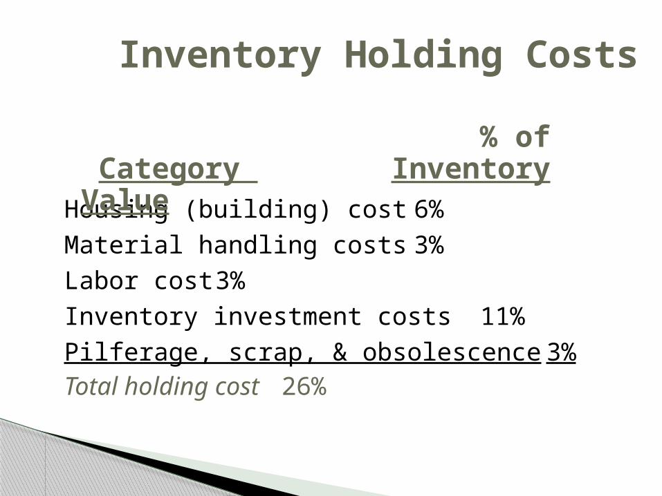
Inventory Holding Costs
Housing (building) cost 6%Material handling costs 3%Labor cost 3%Inventory investment costs 11%Pilferage, scrap, & obsolescence 3%Total holding cost 26%
% of Category Inventory Value
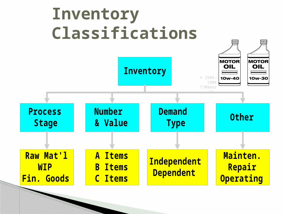
Inventory
ProcessStage
DemandType
Number& Value
Other
Raw Mat'lWIP
Fin. Goods
IndependentDependent
A ItemsB ItemsC Items
Mainten.Repair
Operating
Inventory Classifications
© 1984-1994
T/Maker Co.
Inventory Management
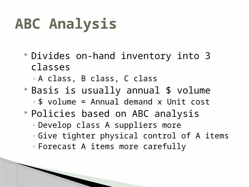
ABC Analysis
Divides on-hand inventory into 3 classes◦ A class, B class, C class
Basis is usually annual $ volume◦ $ volume = Annual demand x Unit cost
Policies based on ABC analysis◦ Develop class A suppliers more◦ Give tighter physical control of A items◦ Forecast A items more carefully
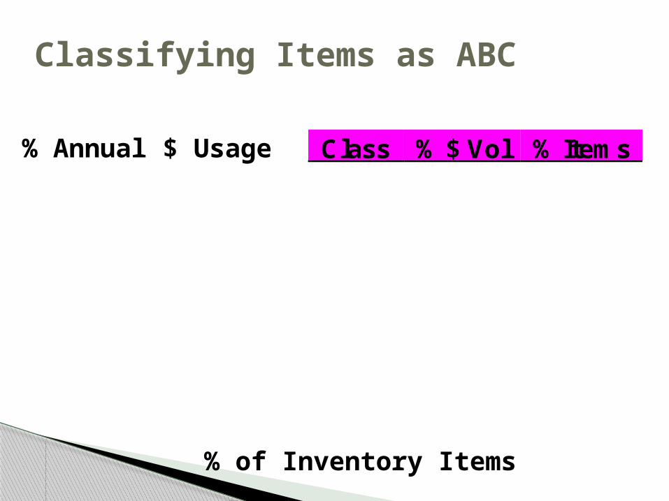
Classifying Items as ABC
0
20
40
60
80
100
0 20 40 60 80 100
% of Inventory Items
% Annual $ Usage Class % $ Vol % Items
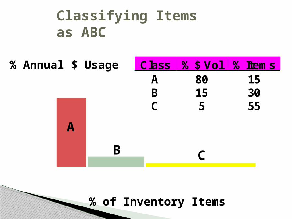
Classifying Items as ABC
0
20
40
60
80
100
0 20 40 60 80 100
% of Inventory Items
% Annual $ Usage
A
B C
Class % $ Vol % ItemsA 80 15B 15 30C 5 55
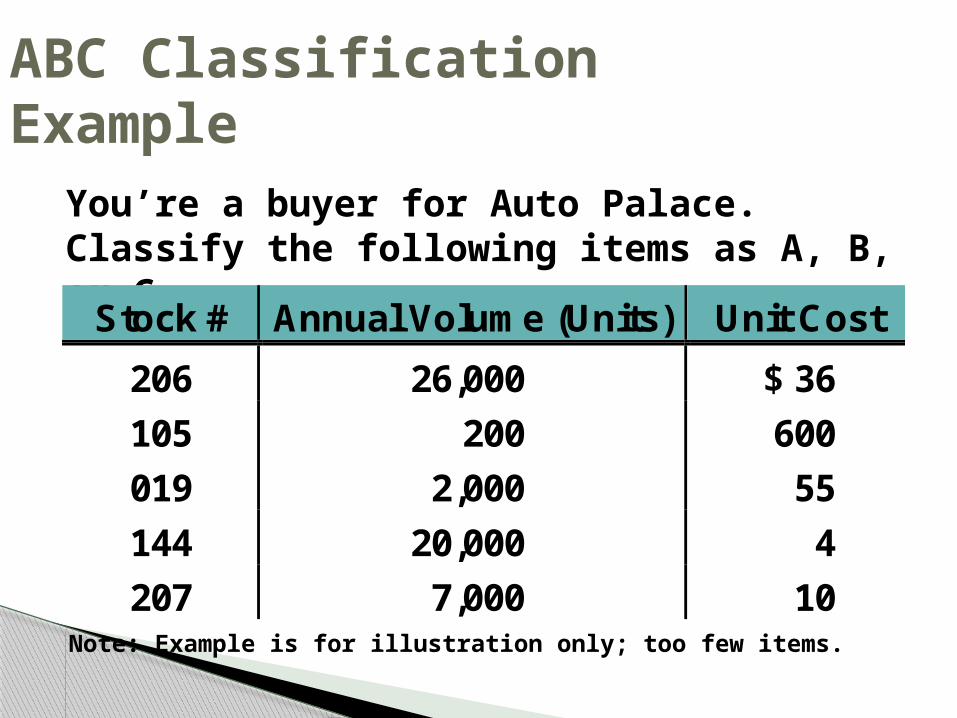
ABC Classification Example
You’re a buyer for Auto Palace. Classify the following items as A, B, or C.
Stock # Annual Volume (Units) Unit Cost
206 26,000 $ 36
105 200 600
019 2,000 55
144 20,000 4
207 7,000 10Note: Example is for illustration only; too few items.

ABC Classification Solution
Stock # Vol. Cost $ Vol. % ABC
206 26,000 $ 36 $936,000 71.1 A
105 200 600 120,000 9.1 A
019 2,000 55 110,000 8.4 B
144 20,000 4 80,000 6.1 B
207 7,000 10 70,000 5.3 C
Total 1,316,000 100.0
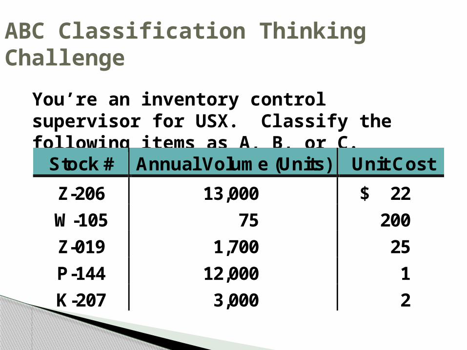
ABC Classification Thinking Challenge
You’re an inventory control supervisor for USX. Classify the following items as A, B, or C.
Stock # Annual Volume (Units) Unit Cost
Z-206 13,000 $ 22
W-105 75 200
Z-019 1,700 25
P-144 12,000 1
K-207 3,000 2
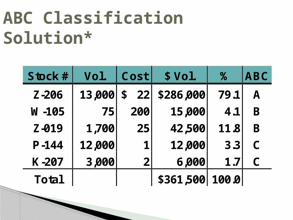
ABC Classification Solution*
Stock # Vol. Cost $ Vol. % ABC
Z-206 13,000 $ 22 $286,000 79.1 A
W-105 75 200 15,000 4.1 B
Z-019 1,700 25 42,500 11.8 B
P-144 12,000 1 12,000 3.3 C
K-207 3,000 2 6,000 1.7 C
Total $361,500 100.0
Physically counting a sample of total inventory on a regular basis
Used often with ABC classification A items counted most often
(e.g., daily)
Cycle Counting

Advantages of Cycle Counting Eliminates shutdown and
interruption of production necessary for annual physical inventories
Eliminates annual inventory adjustments
Provides trained personnel to audit the accuracy of inventory
Allows the cause of errors to be identified and remedial action to be taken
Maintains accurate inventory records
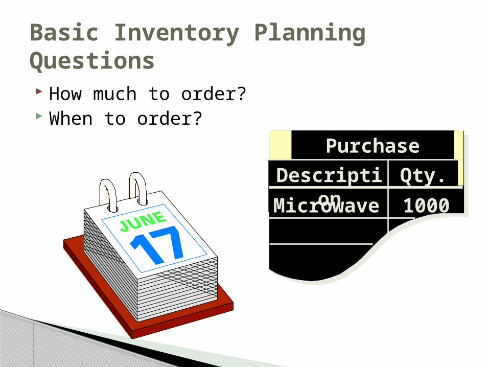
Basic Inventory Planning Questions How much to order? When to order?
Purchase OrderDescripti
onQty.
Microwave
1000

Inventory Models
Fixed order quantity models◦ Economic order quantity◦ Production order quantity◦ Quantity discount
Help answer the inventory planning questions!
Help answer the inventory planning questions!
© 1984-1994 T/Maker Co.
Economic Order Quantity (EOQ) Model
EOQ Assumptions
Known & constant demand Known & constant lead time Instantaneous receipt of material No quantity discounts Only order (setup) cost & holding cost No stockouts
Goal of an Inventory System
Minimize Total Cost (TC)
TC = Holding + Order/Setup Cost
TC = H + S
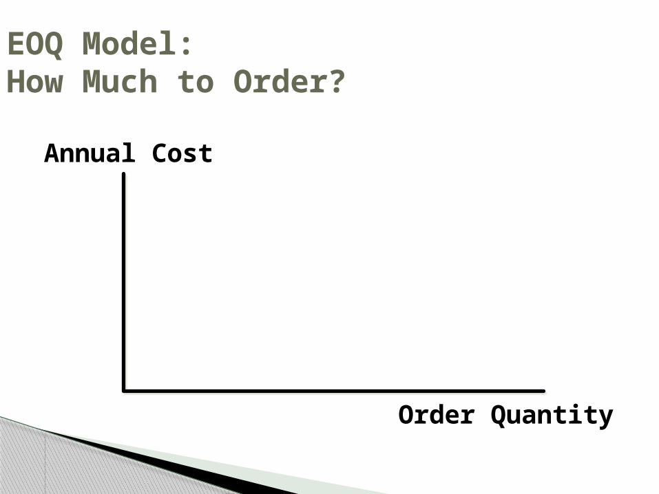
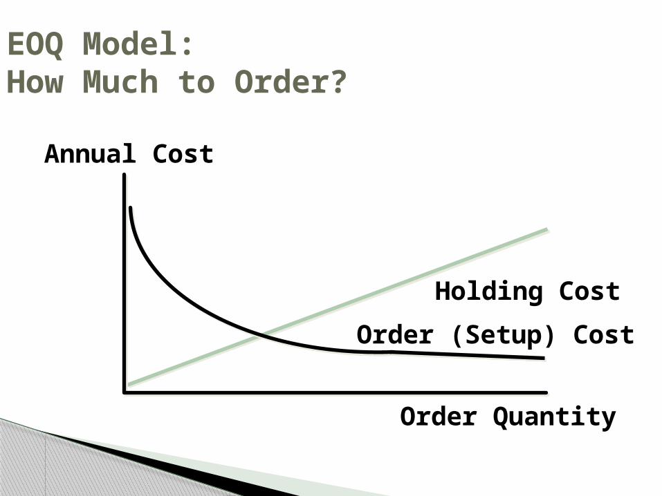
EOQ Model: How Much to Order?
Order Quantity
Annual Cost
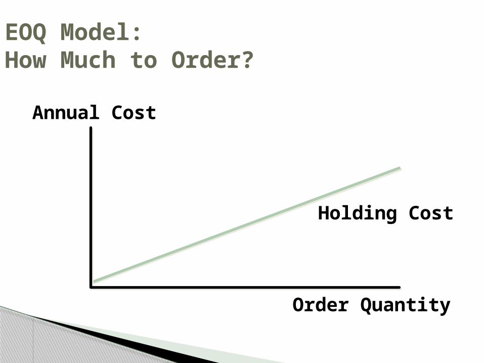
EOQ Model: How Much to Order?
Order Quantity
Annual Cost
Holding Cost
EOQ Model: How Much to Order?
Order Quantity
Annual Cost
Holding Cost
Order (Setup) Cost
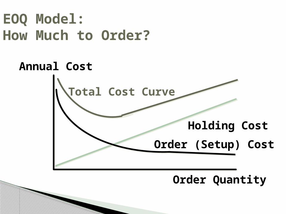
EOQ Model: How Much to Order?
Order Quantity
Annual Cost
Holding Cost
Total Cost Curve
Order (Setup) Cost
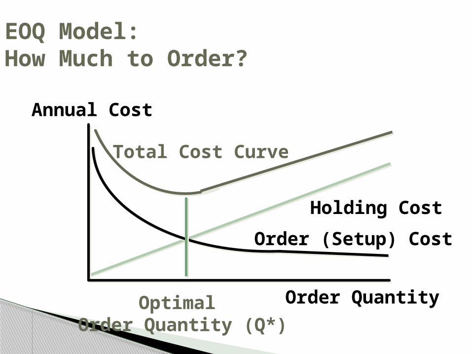
EOQ Model: How Much to Order?
Order Quantity
Annual Cost
Holding Cost
Total Cost Curve
Order (Setup) Cost
Optimal Order Quantity (Q*)
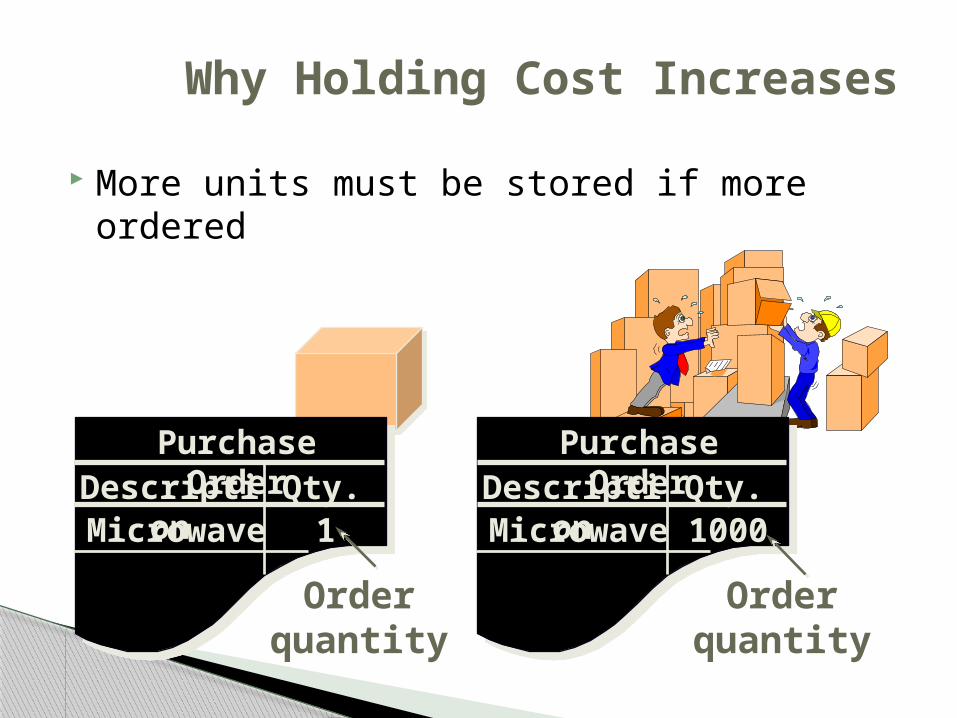
Why Holding Cost Increases
More units must be stored if more ordered
Purchase OrderDescripti
onQty.
Microwave
1000
Purchase OrderDescripti
onQty.
Microwave
1
Order quantity
Order quantity
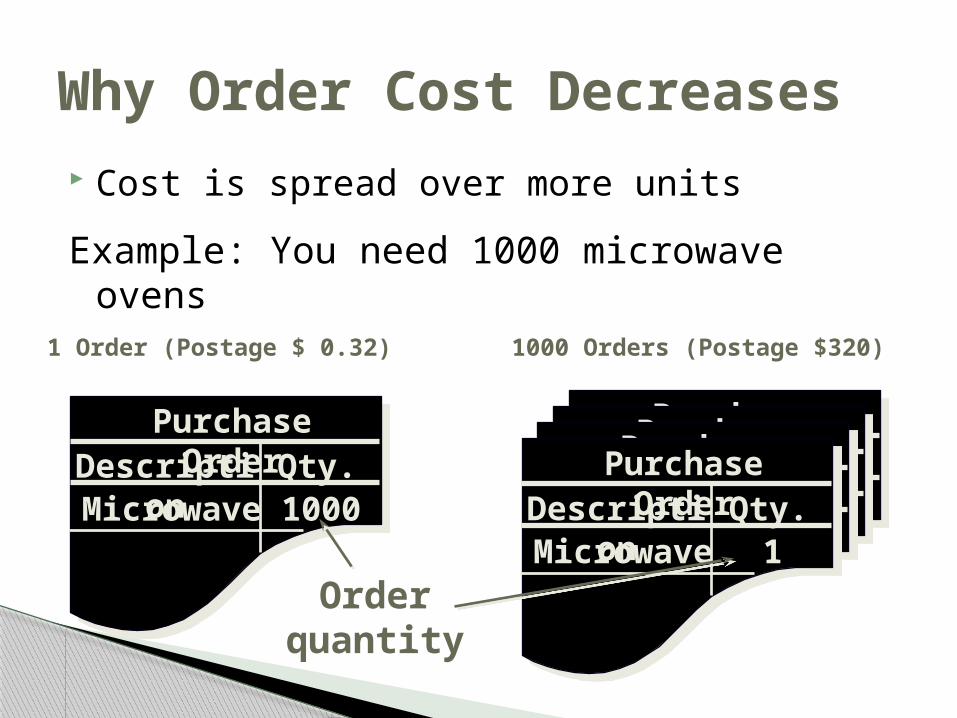
Why Order Cost Decreases Cost is spread over more units
Example: You need 1000 microwave ovens
Purchase OrderDescripti
onQty.
Microwave
1000
Purchase OrderDescripti
onQty.
Microwave
1
Purchase OrderDescripti
onQty.
Microwave
1
Purchase OrderDescripti
onQty.
Microwave
1
Purchase OrderDescripti
onQty.
Microwave
1
1 Order (Postage $ 0.32) 1000 Orders (Postage $320)
Order quantity
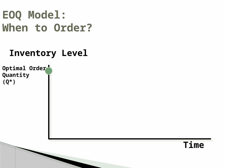
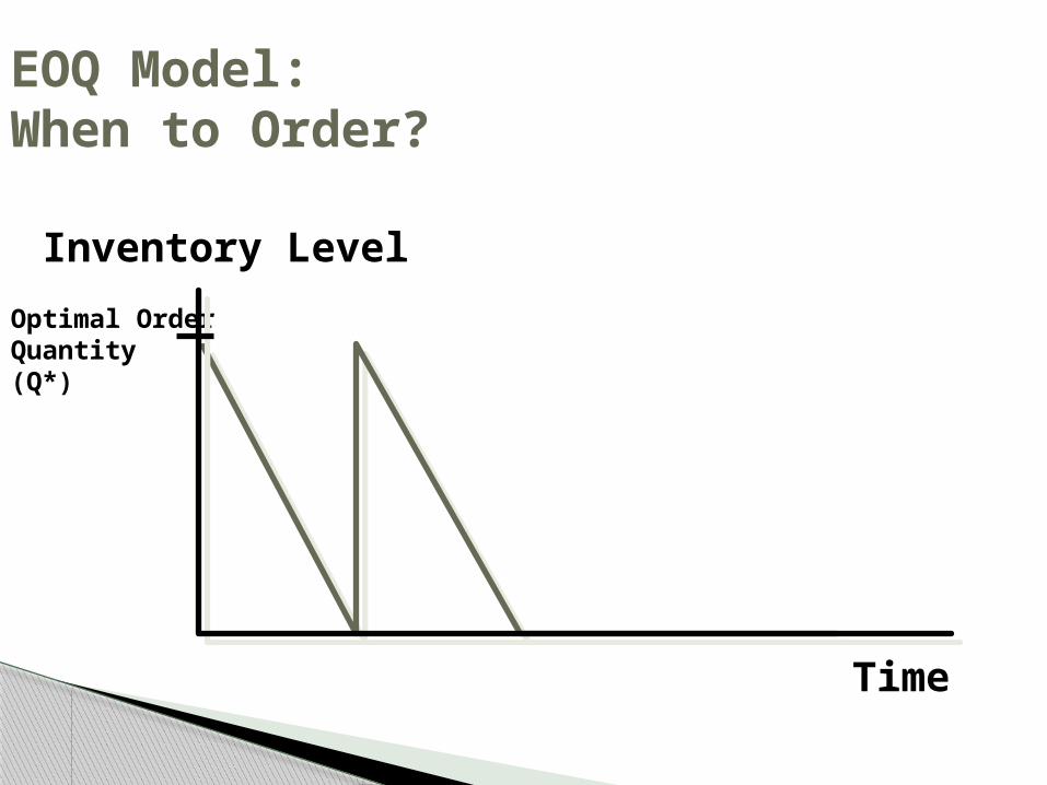
EOQ Model: When to Order?
Inventory Level
Optimal Order Quantity (Q*)
Time
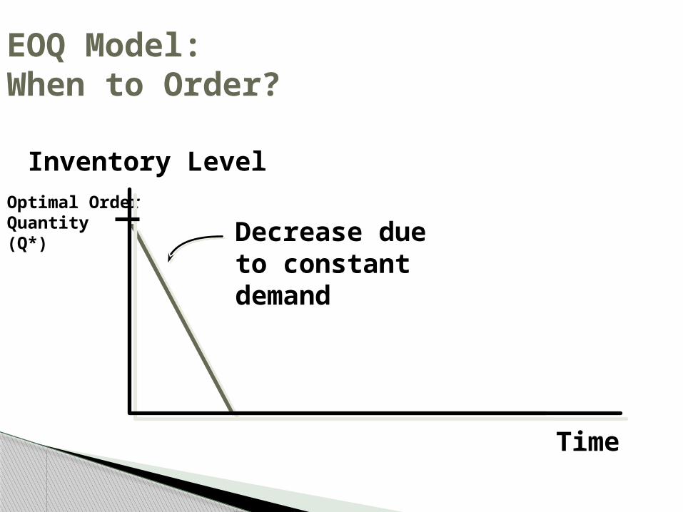
EOQ Model: When to Order?
Inventory LevelOptimal Order Quantity (Q*) Decrease due
to constant demand
Time
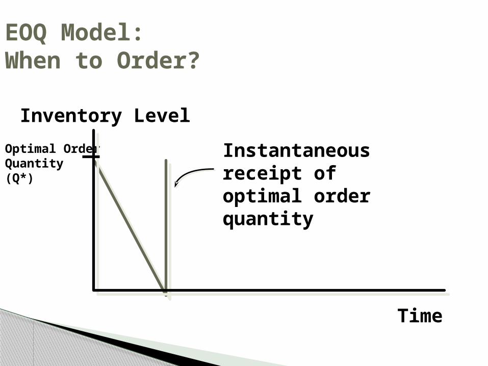
EOQ Model: When to Order?
Inventory Level
Optimal Order Quantity (Q*)
Instantaneous receipt of optimal order quantity
Time
EOQ Model: When to Order?
Inventory Level
Optimal Order Quantity (Q*)
Time

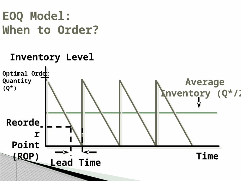
EOQ Model: When to Order?
Inventory LevelOptimal Order Quantity (Q*)
Lead Time
Reorder
Point (ROP) Time
Reorder
Point (ROP)
EOQ Model: When to Order?
Time
Inventory Level
Optimal Order Quantity(Q*)
AverageInventory (Q*/2)
Lead Time
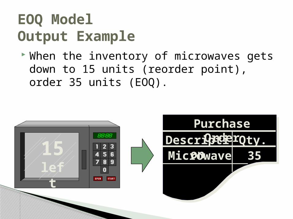
EOQ Model Output Example When the inventory of microwaves gets
down to 15 units (reorder point), order 35 units (EOQ).
15 left
Purchase OrderDescripti
onQty.
Microwave
35
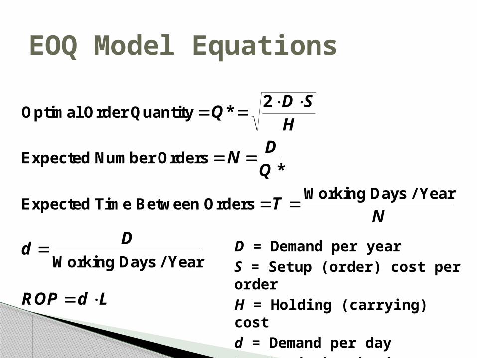
EOQ Model Equations
Optimal Order Quantity
Expected Number Orders
Expected Time Between OrdersWorking Days / Year
Working Days / Year
QD SH
NDQ
TN
dD
ROP d L
*
*
2
D = Demand per yearS = Setup (order) cost per orderH = Holding (carrying) cost d = Demand per dayL = Lead time in days
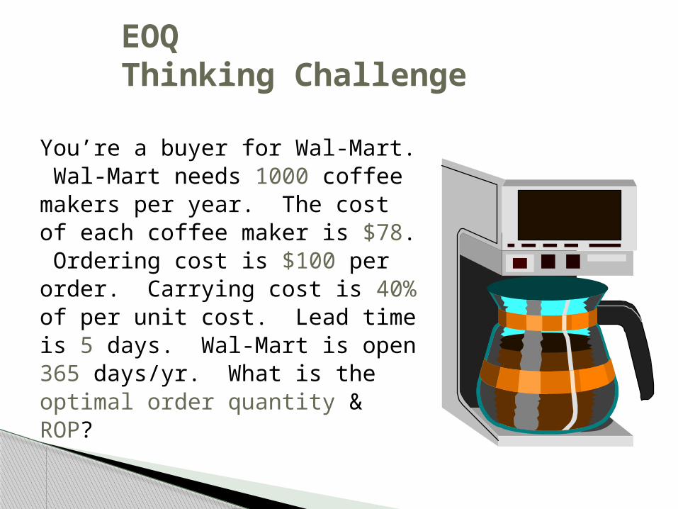
EOQ Thinking Challenge
You’re a buyer for Wal-Mart. Wal-Mart needs 1000 coffee makers per year. The cost of each coffee maker is $78. Ordering cost is $100 per order. Carrying cost is 40% of per unit cost. Lead time is 5 days. Wal-Mart is open 365 days/yr. What is the optimal order quantity & ROP?

EOQ Model Equations
Optimal Order Quantity
Expected Number Orders
Expected Time Between OrdersWorking Days / Year
Working Days / Year
QD SH
NDQ
TN
dD
ROP d L
*
*
2
D = Demand per yearS = Setup (order) cost per orderH = Holding (carrying) cost d = Demand per dayL = Lead time in days
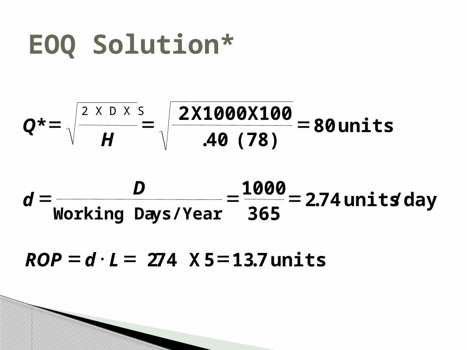
EOQ Solution*
QH
dD
ROP d L
*.
.
. .
= = =
= = =
= × = =
2X1000X10040 (78)
80
1000365
274
274 X 5 137
units
units/day
units
Working Days/Year
2 X D X S
Production Order Quantity Model
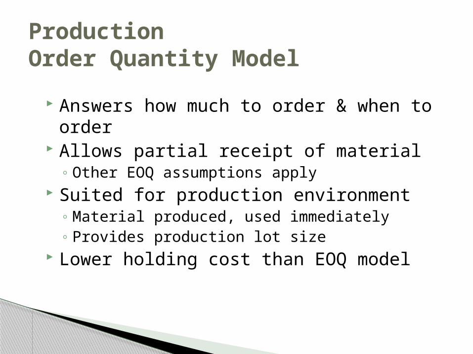
Production Order Quantity Model
Answers how much to order & when to order
Allows partial receipt of material◦ Other EOQ assumptions apply
Suited for production environment◦ Material produced, used immediately◦ Provides production lot size
Lower holding cost than EOQ model

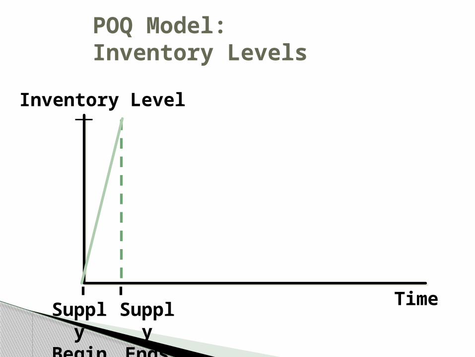
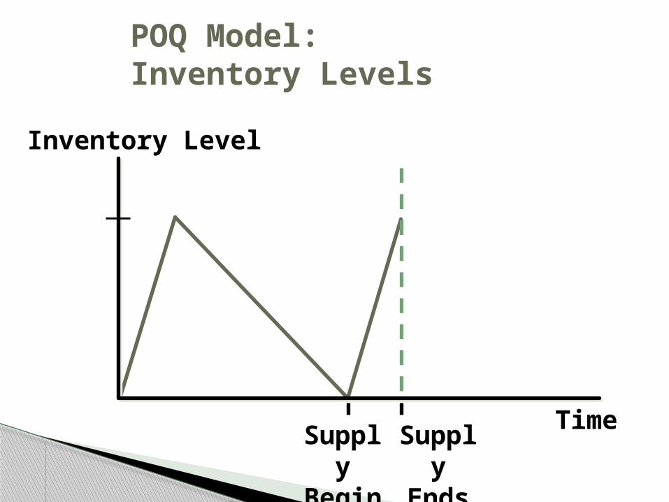
POQ Model: Inventory Levels
Time
Inventory Level
Supply
Begins
POQ Model: Inventory Levels
Time
Inventory Level
Supply
Begins
Supply
Ends
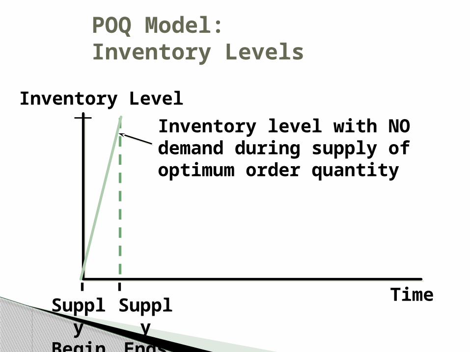
POQ Model: Inventory Levels
Time
Inventory Level
Supply
Begins
Supply
Ends
Inventory level with NO demand during supply of optimum order quantity
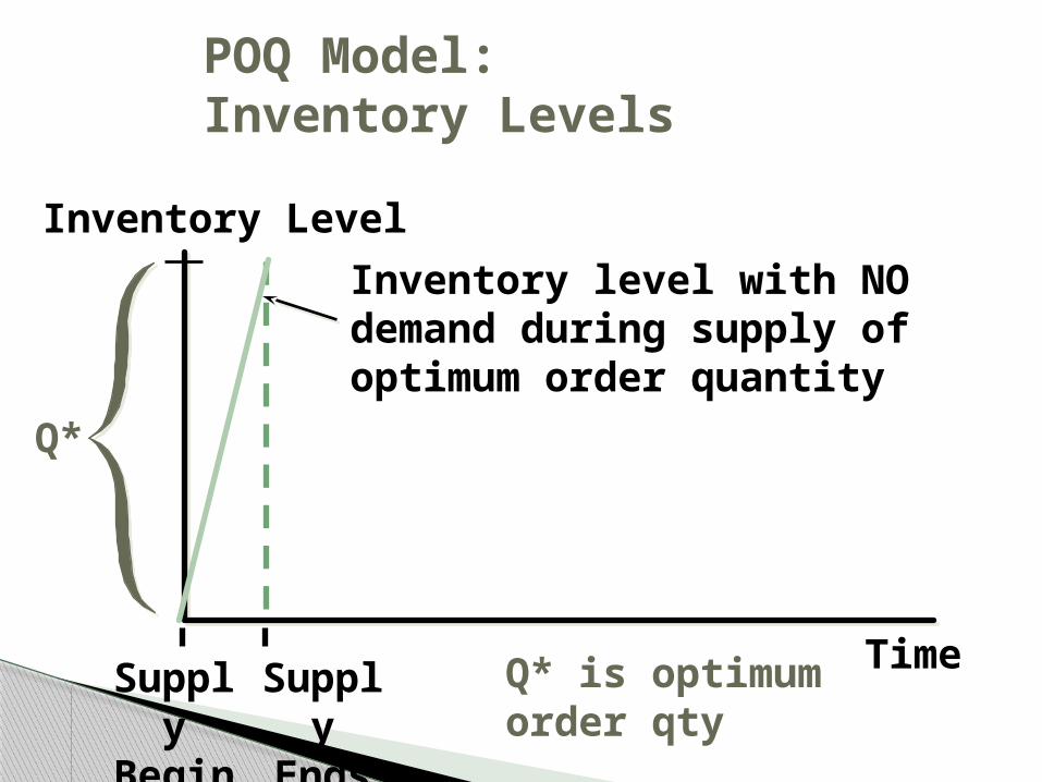
POQ Model: Inventory Levels
Time
Inventory Level
Supply
Begins
Supply
Ends
Inventory level with NO demand during supply of optimum order quantity
Q*
Q* is optimum order qty
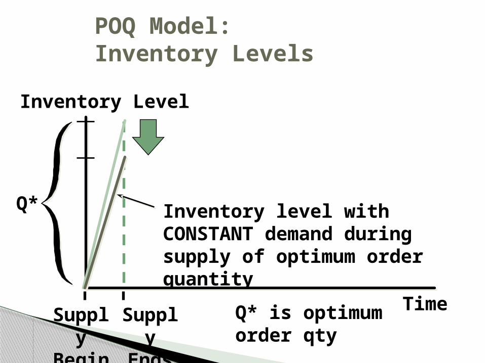
POQ Model: Inventory Levels
Time
Inventory Level
Supply
Begins
Supply
Ends
Inventory level with CONSTANT demand during supply of optimum order quantity
Q*
Q* is optimum order qty
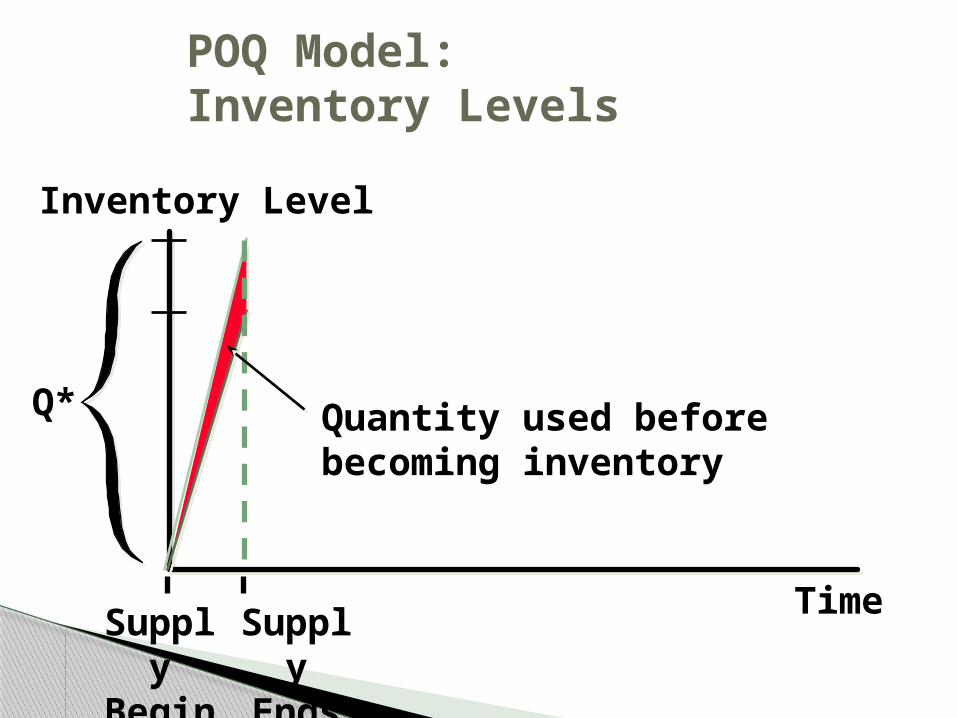
POQ Model: Inventory Levels
Time
Inventory Level
Supply
Begins
Supply
Ends
Q* Quantity used before becoming inventory
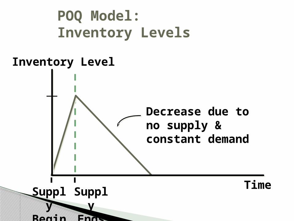
POQ Model: Inventory Levels
Time
Inventory Level
Supply
Begins
Supply
Ends
Decrease due to no supply & constant demand

Inventory Level
POQ Model: Inventory Levels
TimeSuppl
y Begin
s
Supply
Ends
Production portion of cycle
Demand portion of cycle with no supply
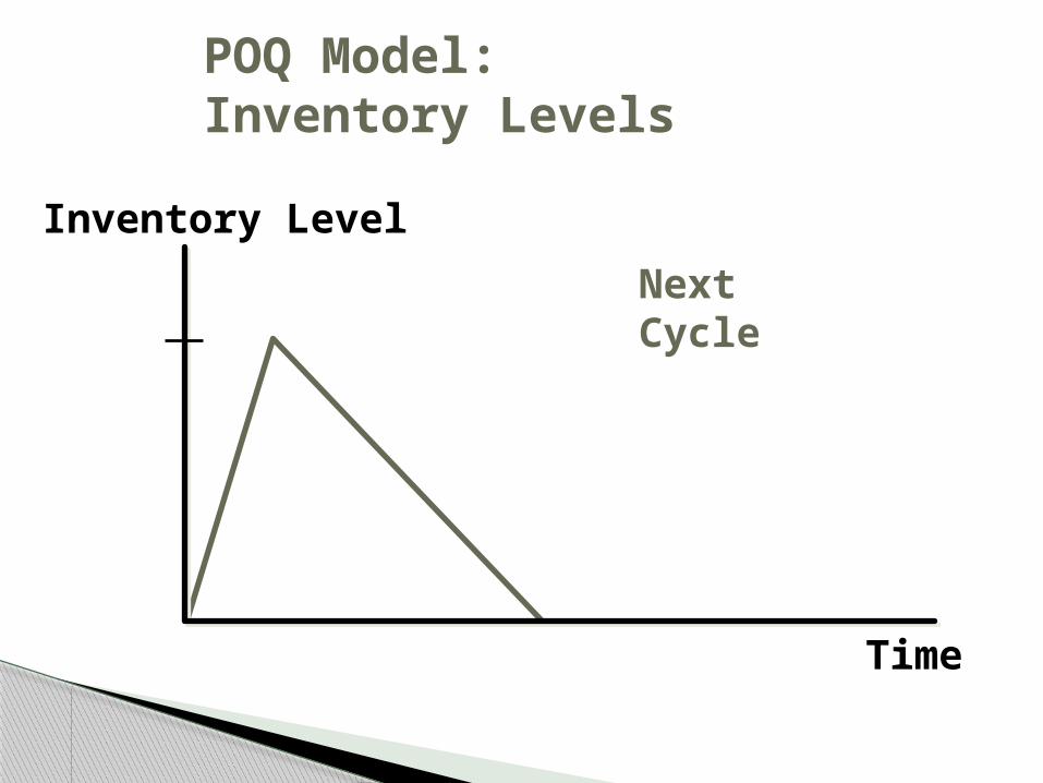
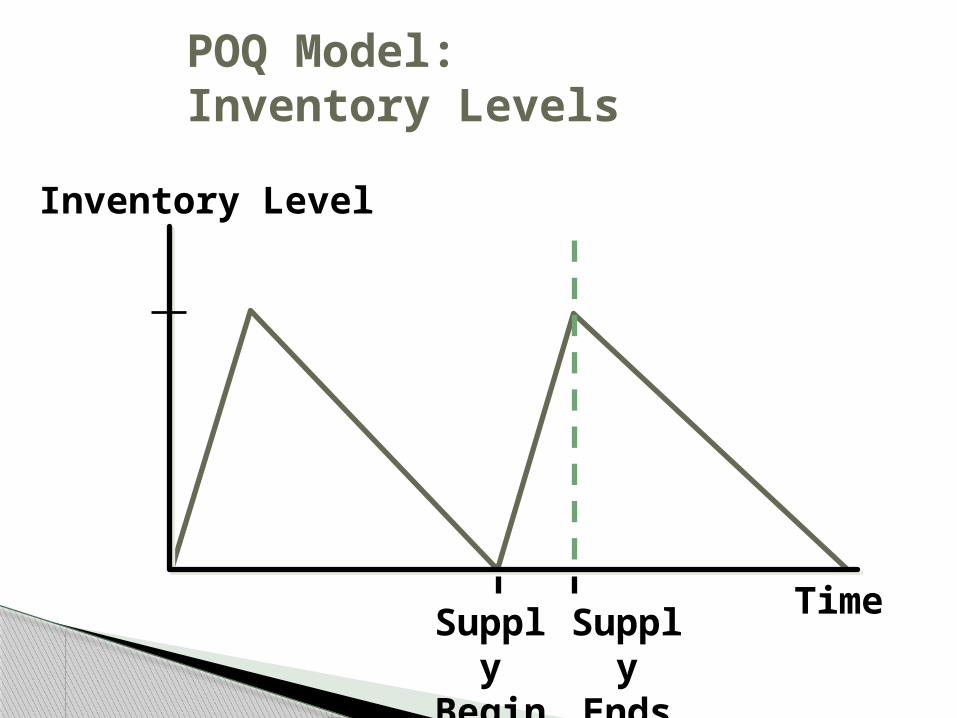
POQ Model: Inventory Levels
Time
Inventory Level
Next Cycle
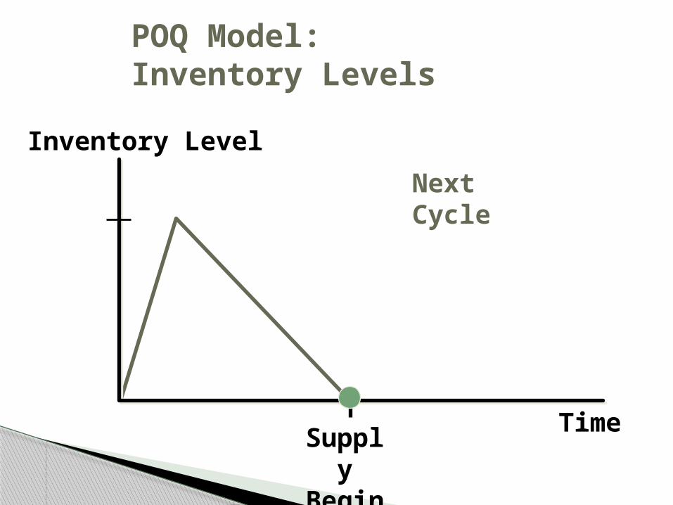
POQ Model: Inventory Levels
Time
Inventory Level
Supply
Begins
Next Cycle
POQ Model: Inventory Levels
Time
Inventory Level
Supply
Begins
Supply
Ends
POQ Model: Inventory Levels
Time
Inventory Level
Supply
Begins
Supply
Ends
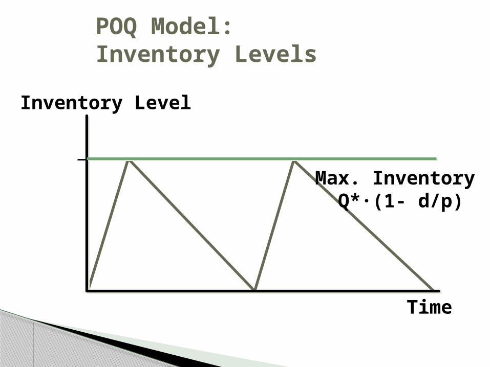
POQ Model: Inventory Levels
Time
Inventory Level
Max. Inventory Q*·(1- d/p)
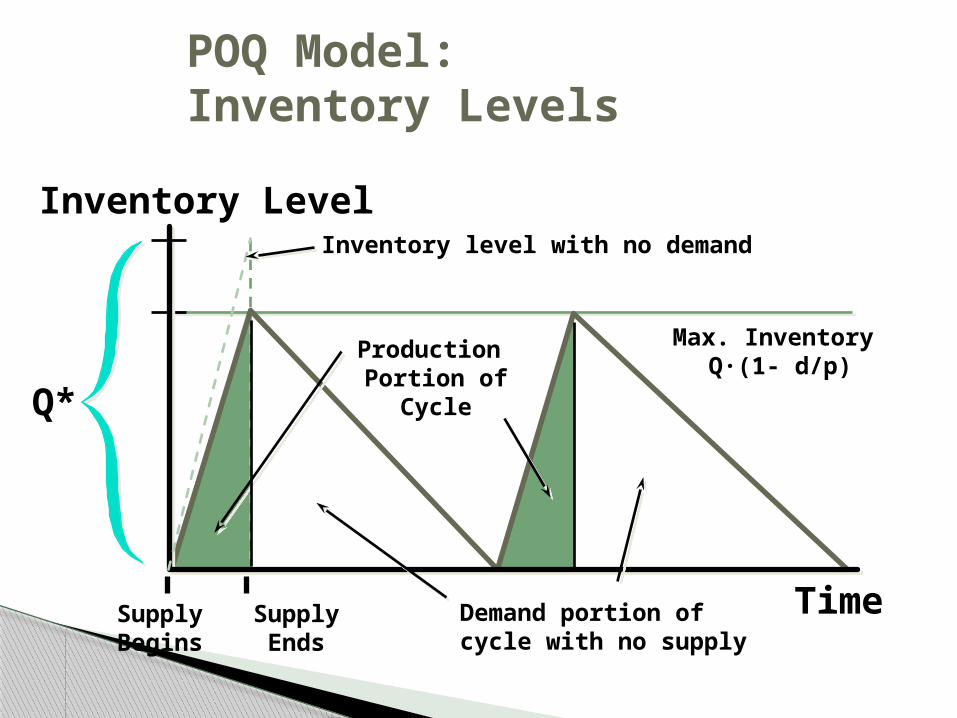
POQ Model: Inventory Levels
Time
Inventory Level
Production Portion of Cycle
Max. Inventory Q·(1- d/p)
Q*
Supply Begins
Supply Ends
Inventory level with no demand
Demand portion of cycle with no supply
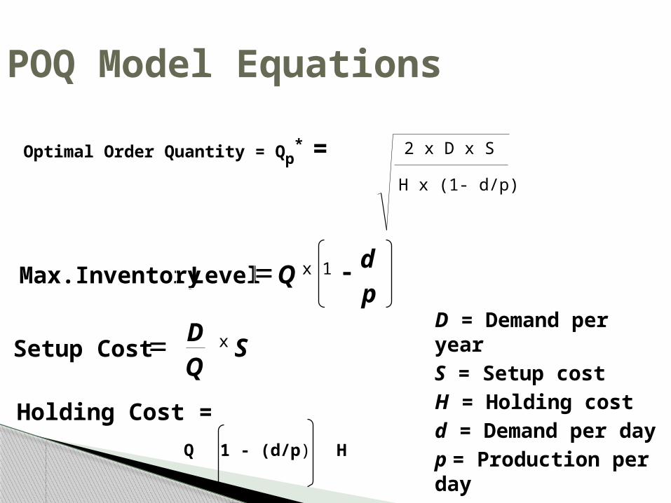
POQ Model Equations
Max. Inventory Level
Setup Cost
Holding Cost =
= -
=
Qdp
DQ
SD = Demand per yearS = Setup costH = Holding cost d = Demand per dayp = Production per day
Optimal Order Quantity = Qp* = 2 x D x S
H x (1- d/p)
x 1
x
Q 1 - (d/p) H
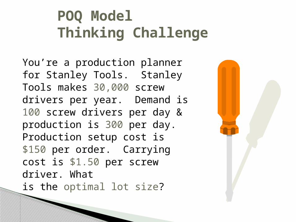
POQ Model Thinking Challenge
You’re a production planner for Stanley Tools. Stanley Tools makes 30,000 screw drivers per year. Demand is 100 screw drivers per day & production is 300 per day. Production setup cost is $150 per order. Carrying cost is $1.50 per screw driver. What is the optimal lot size?

POQ Model Equations
Max. Inventory Level
Setup Cost
Holding Cost =
= -
=
Qdp
DQ
SD = Demand per yearS = Setup costH = Holding cost d = Demand per dayp = Production per day
Optimal Order Quantity = Qp* = 2 x D x S
H x (1- d/p)
x 1
x
Q 1 - (d/p) H
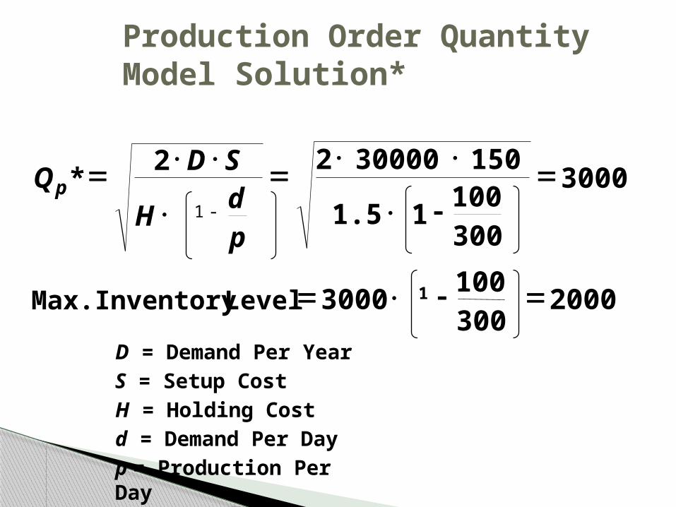
Production Order Quantity Model Solution*
QD S
Hdp
p*=× ×
×=
× ×
× -=
= × - =
2 2 30000 150
1.5 1100300
3000
3000100300
2000Max. Inventory Level
D = Demand Per YearS = Setup CostH = Holding Cost d = Demand Per Dayp = Production Per Day
1 -
1
Quantity Discount Model
Answers how much to order & when to order
Allows quantity discounts◦ Reduced price when item is purchased in larger
quantities◦ Other EOQ assumptions apply
Trade-off is between lower price & increased holding cost
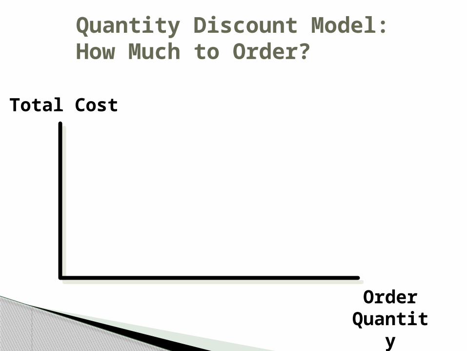
Quantity Discount Model: How Much to Order?
Order Quantit
y
Total Cost
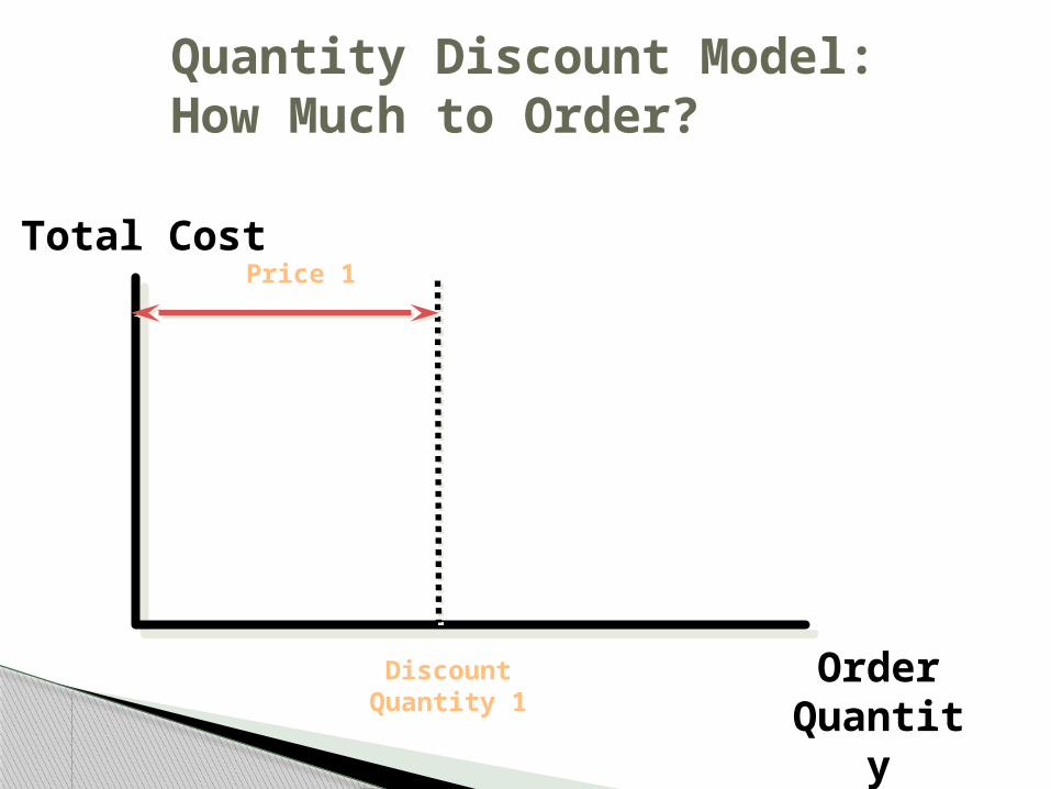
Quantity Discount Model: How Much to Order?
Order Quantit
y
Total Cost
Discount Quantity 1
Price 1
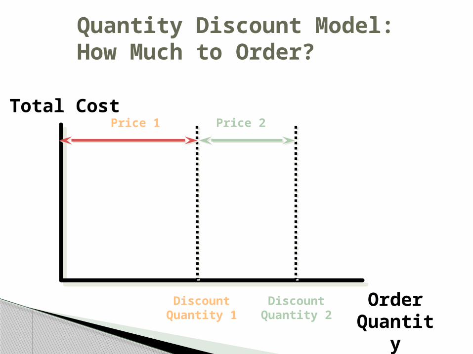
Quantity Discount Model: How Much to Order?
Order Quantit
y
Total Cost
Discount Quantity 1
Discount Quantity 2
Price 1 Price 2
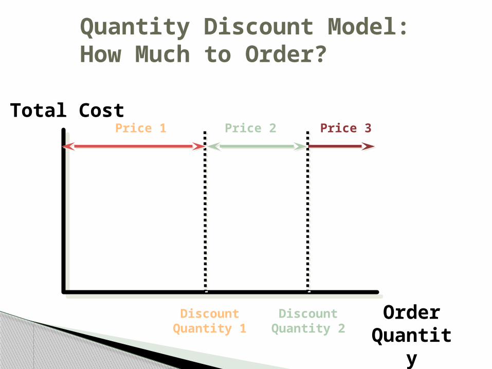
Order Quantit
y
Quantity Discount Model: How Much to Order?
Total Cost
Discount Quantity 1
Discount Quantity 2
Price 1 Price 2 Price 3
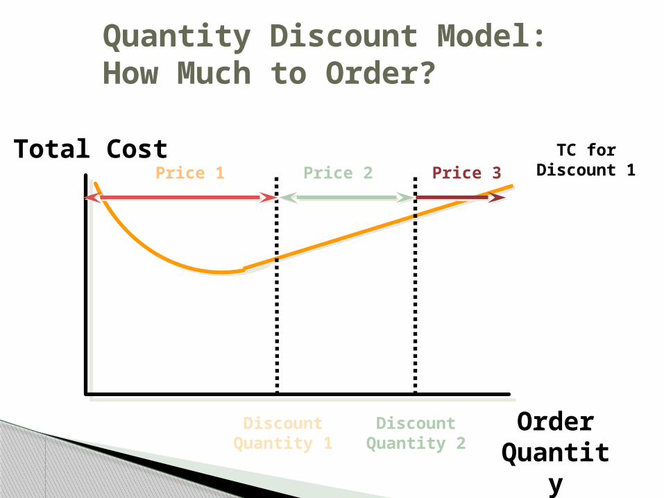
Quantity Discount Model: How Much to Order?
Order Quantit
y
Total Cost TC for Discount 1
Discount Quantity 1
Discount Quantity 2
Price 1 Price 2 Price 3

Quantity Discount Model: How Much to Order?
Order Quantit
y
Total Cost TC for Discount 1
Discount Quantity 1
Discount Quantity 2
Price 1 Price 2 Price 3
Q*

Quantity Discount Model: How Much to Order?
Order Quantit
y
Total Cost TC for Discount 1
Discount Quantity 1
Discount Quantity 2
Price 1 Price 2 Price 3
Q*
Outside discount range
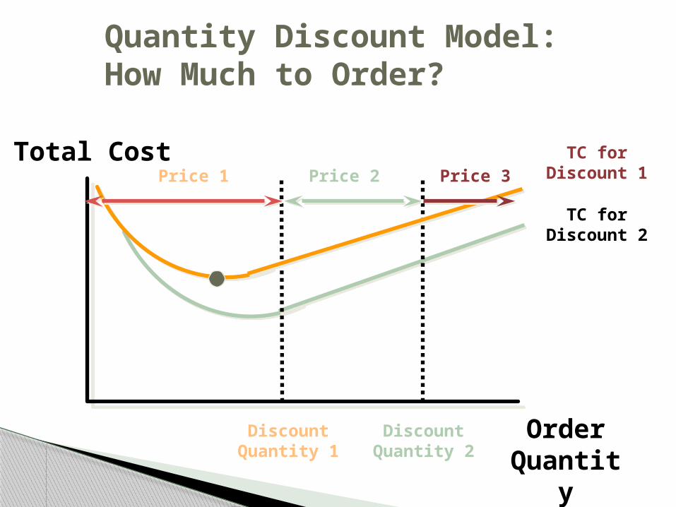
Quantity Discount Model: How Much to Order?
Order Quantit
y
Total Cost
Discount Quantity 1
TC for Discount 2
Discount Quantity 2
Price 1 Price 2 Price 3TC for
Discount 1

Quantity Discount Model: How Much to Order?
Order Quantit
y
Total Cost
Disc Qty 1
TC for Discount 2
Discount Quantity 2
Price 1 Price 2 Price 3
Q*
TC for Discount 1

Quantity Discount Model: How Much to Order?
Order Quantit
y
Total Cost
Disc Qty 1
TC for Discount 2
Discount Quantity 2
Price 1 Price 2 Price 3
Q*
Outside discount range
Outside discount range
TC for Discount 1
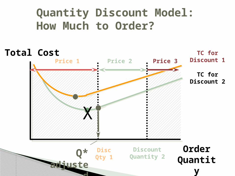
Quantity Discount Model: How Much to Order?
Order Quantit
y
Total Cost
Disc Qty 1
TC for Discount 2
Discount Quantity 2
Price 1 Price 2 Price 3
Q* adjuste
d
TC for Discount 1
X
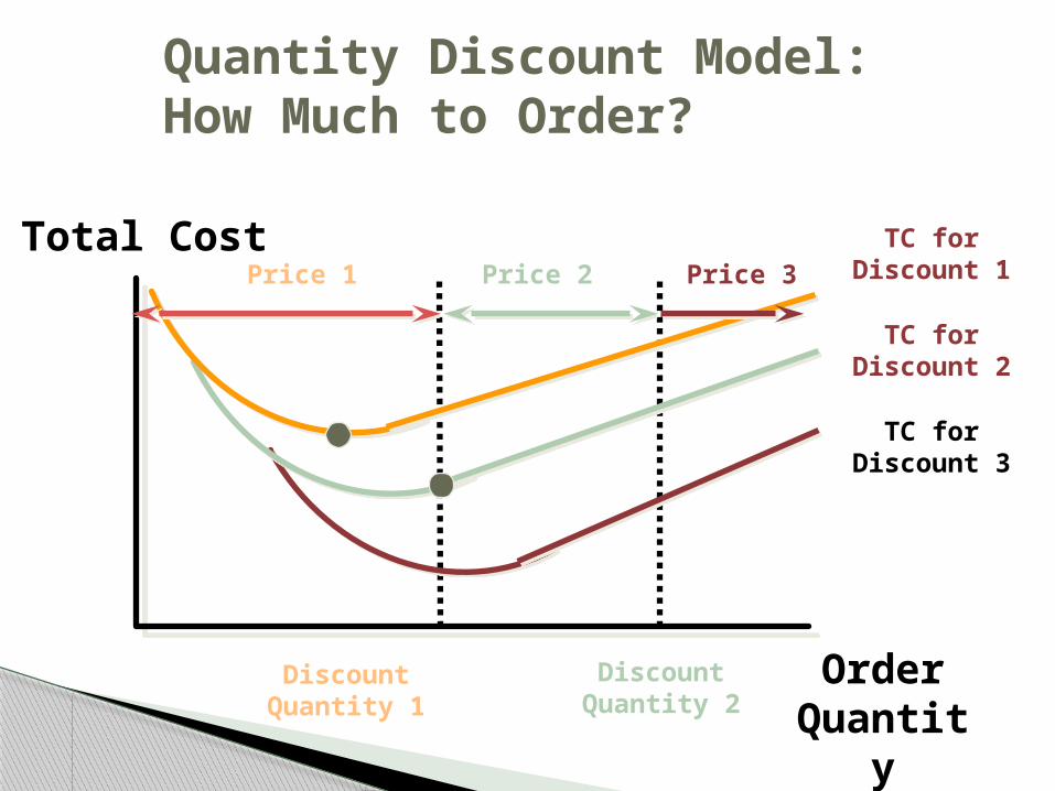
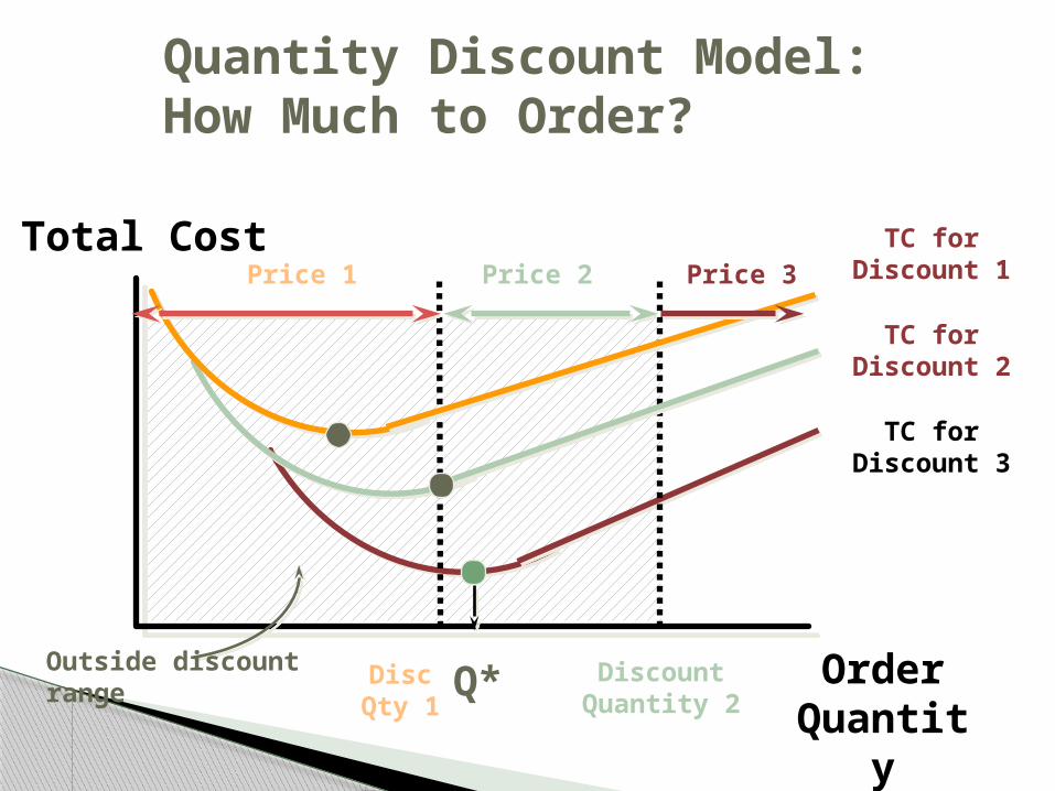
Quantity Discount Model: How Much to Order?
Order Quantit
y
Total Cost
TC for Discount 3
Discount Quantity 2
Price 1 Price 2 Price 3
Discount Quantity 1
TC for Discount 2
TC for Discount 1

Quantity Discount Model: How Much to Order?
Order Quantit
y
Total Cost
TC for Discount 3
Discount Quantity 2
Price 1 Price 2 Price 3
Q*Discount Quantity 1
TC for Discount 2
TC for Discount 1
Quantity Discount Model: How Much to Order?
Order Quantit
y
Total Cost
TC for Discount 3
Discount Quantity 2
Price 1 Price 2 Price 3
Disc Qty 1
Outside discount range Q*
TC for Discount 2
TC for Discount 1
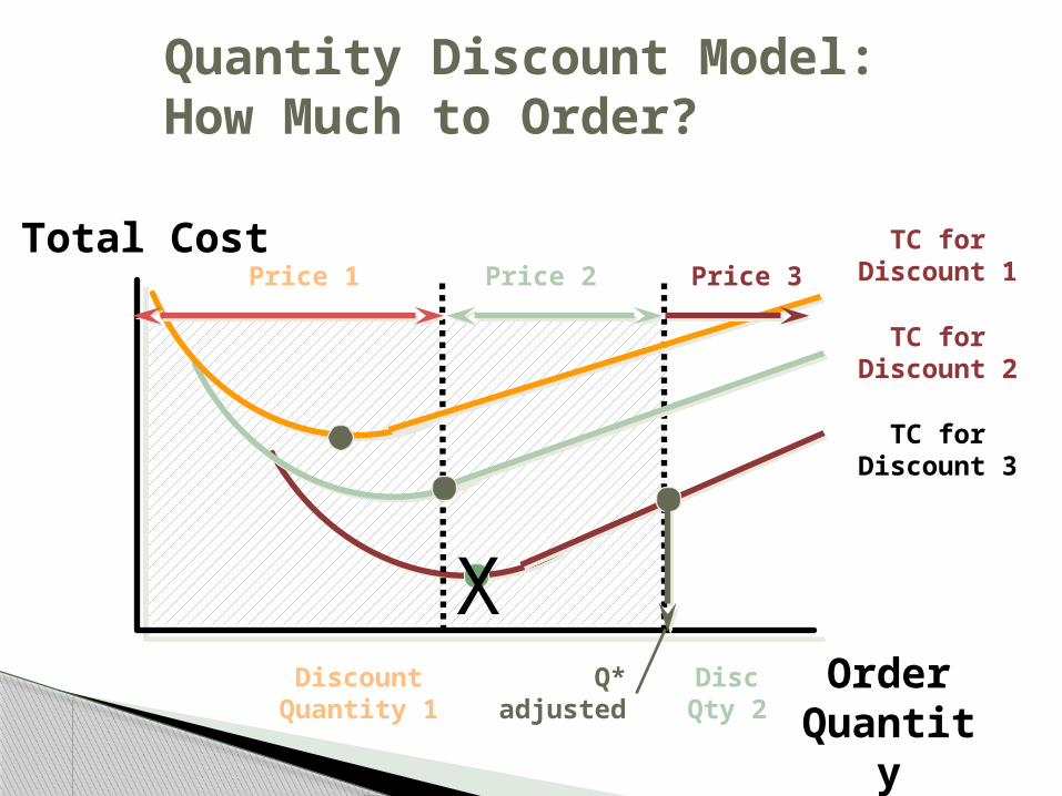
Quantity Discount Model: How Much to Order?
Order Quantit
y
Total Cost
TC for Discount 3
Disc Qty 2
Price 1 Price 2 Price 3
Q* adjusted
Discount Quantity 1
X
TC for Discount 2
TC for Discount 1
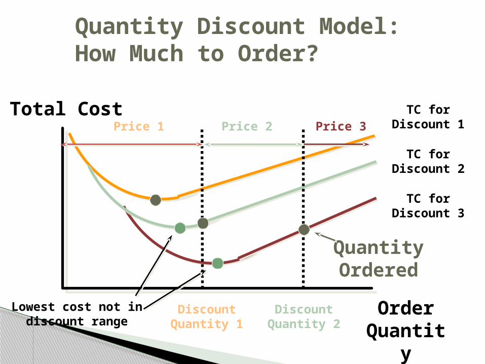
Quantity Discount Model: How Much to Order?
Order Quantit
y
Total Cost TC for Discount 1
Discount Quantity 1
TC for Discount 2
TC for Discount 3
Discount Quantity 2
Lowest cost not in discount range
Quantity Ordered
Price 1 Price 2 Price 3
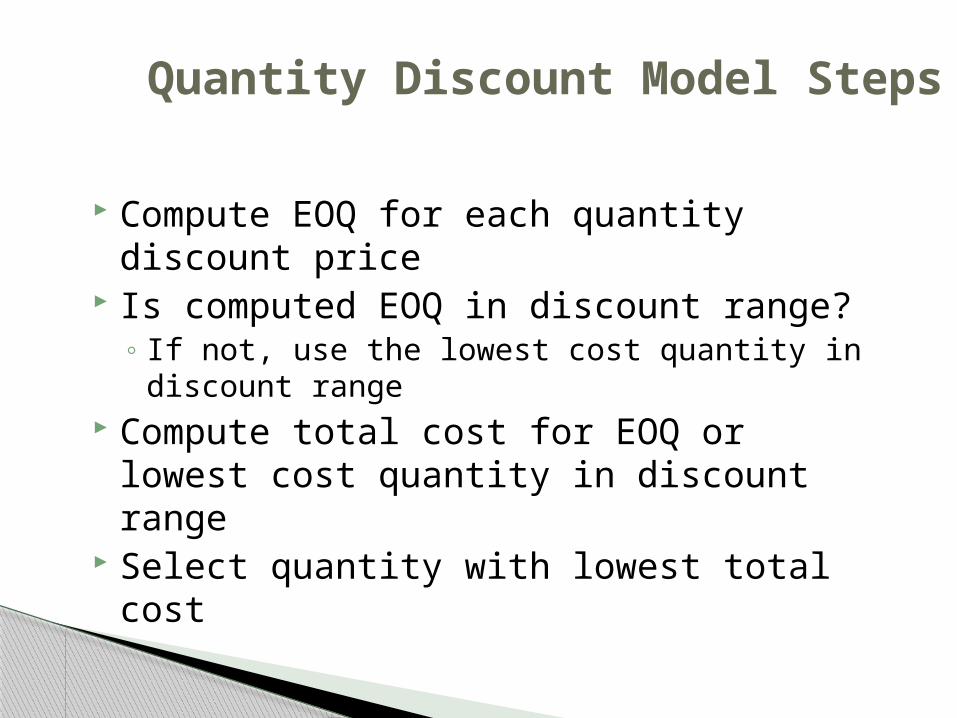
Quantity Discount Model Steps
Compute EOQ for each quantity discount price
Is computed EOQ in discount range?◦ If not, use the lowest cost quantity in discount
range Compute total cost for EOQ or lowest cost
quantity in discount range Select quantity with lowest total cost