Jolly Pochie

Technical Report in RoboCup 2006

Hayato Kobayashi1 Jun Inoue1 Tsugutoyo Osaki2

Tetsuro Okuyama2 Shuhei Yanagimachi2 Takahito Sasaki2

Keisuke Oi2 Seiji Hirama2 Akira Ishino2

Ayumi Shinohara2 Akihiro Kamiya 2 Satoshi Abe2

Wataru Matsubara2 Tomoyuki Nakamura2

1 Department of Informatics, Kyushu University2 Department of System Information Sciences, GSIS, Tohoku University

January 15, 2007

Contents

1 Introduction 3

2 Vision 52.1 Object Recognition . . . . . . . . . . . . . . . . . . . . . . . . . 8

2.1.1 Ball Recognition . . . . . . . . . . . . . . . . . . . . . . 92.1.2 Landmark Recognition . . . . . . . . . . . . . . . . . . . 9

2.2 Player Recognition . . . . . . . . . . . . . . . . . . . . . . . . . 10

3 Ball Localization 123.1 Introduction . . . . . . . . . . . . . . . . . . . . . . . . . . . . . 123.2 Ball Recognition from the Image Data . . . . . . . . . . . . . . . 123.3 Ball Localization using Monte-Carlo Method . . . . . . . . . . . 14

3.3.1 Ball Monte-Carlo localization updated by only position in-formation . . . . . . . . . . . . . . . . . . . . . . . . . . 14

3.3.2 Ball Monte-Carlo localization updated by position and ve-locity information . . . . . . . . . . . . . . . . . . . . . 16

3.3.3 Ball Monte-Carlo localization with two sets of samples . . 173.3.4 On the number of samples . . . . . . . . . . . . . . . . . 173.3.5 Real-world Experiments . . . . . . . . . . . . . . . . . . 17

3.4 Conclusions . . . . . . . . . . . . . . . . . . . . . . . . . . . . . 20

4 Learning of Ball Trapping 214.1 Introduction . . . . . . . . . . . . . . . . . . . . . . . . . . . . . 214.2 Preliminary . . . . . . . . . . . . . . . . . . . . . . . . . . . . . 22

4.2.1 Ball Trapping . . . . . . . . . . . . . . . . . . . . . . . . 224.2.2 One-dimensional Model of Ball Trapping . . . . . . . . . 23

4.3 Training Equipment . . . . . . . . . . . . . . . . . . . . . . . . . 244.4 Learning Method . . . . . . . . . . . . . . . . . . . . . . . . . . 244.5 Experiments . . . . . . . . . . . . . . . . . . . . . . . . . . . . . 26

4.5.1 Training Using One Robot . . . . . . . . . . . . . . . . . 264.5.2 Training Using Two Robots . . . . . . . . . . . . . . . . 294.5.3 Training Using Two Robots with Communication . . . . . 31

4.6 Discussion . . . . . . . . . . . . . . . . . . . . . . . . . . . . . . 31

1

4.7 Conclusions and Future Work . . . . . . . . . . . . . . . . . . . . 33

5 Strategy System 345.1 Behavior System . . . . . . . . . . . . . . . . . . . . . . . . . . 34

6 Strategies for Jolly Pochie 2006 366.1 Attacker . . . . . . . . . . . . . . . . . . . . . . . . . . . . . . . 36

6.1.1 Search . . . . . . . . . . . . . . . . . . . . . . . . . . . . 366.1.2 Approach . . . . . . . . . . . . . . . . . . . . . . . . . . 376.1.3 Shoot . . . . . . . . . . . . . . . . . . . . . . . . . . . . 376.1.4 Support . . . . . . . . . . . . . . . . . . . . . . . . . . . 376.1.5 Localize . . . . . . . . . . . . . . . . . . . . . . . . . . . 376.1.6 Problems for next year . . . . . . . . . . . . . . . . . . . 38

6.2 Defender . . . . . . . . . . . . . . . . . . . . . . . . . . . . . . 386.3 Goalie . . . . . . . . . . . . . . . . . . . . . . . . . . . . . . . . 39

6.3.1 Position . . . . . . . . . . . . . . . . . . . . . . . . . . . 396.3.2 Search . . . . . . . . . . . . . . . . . . . . . . . . . . . . 406.3.3 Guard . . . . . . . . . . . . . . . . . . . . . . . . . . . . 406.3.4 Clear . . . . . . . . . . . . . . . . . . . . . . . . . . . . 416.3.5 Conclusion . . . . . . . . . . . . . . . . . . . . . . . . . 436.3.6 Problems for Next Year . . . . . . . . . . . . . . . . . . . 43

7 Shot Motions 447.1 Shot with its chest . . . . . . . . . . . . . . . . . . . . . . . . . . 447.2 Shot with its leg . . . . . . . . . . . . . . . . . . . . . . . . . . . 457.3 Shot with its head . . . . . . . . . . . . . . . . . . . . . . . . . . 45

7.3.1 Type1 (when the ball is near) . . . . . . . . . . . . . . . . 467.3.2 Type2 (when the ball is far) . . . . . . . . . . . . . . . . 47

7.4 Shot after catch . . . . . . . . . . . . . . . . . . . . . . . . . . . 47

8 Technical Challenges 488.1 The Open Challenge . . . . . . . . . . . . . . . . . . . . . . . . 488.2 The Passing Challenge . . . . . . . . . . . . . . . . . . . . . . . 488.3 The New Goal Challenge . . . . . . . . . . . . . . . . . . . . . . 48

9 Conclusion 50

2

Chapter 1

Introduction

The team “Jolly Pochie [dzóli·pót∫i:]” has participated in the RoboCup Four-legged

League since 2003. Jolly Pochie consists of the faculty staff and graduate/undergraduatestudents of Department of Informatics, Kyushu University and Department of Sys-tem Information Sciences, GSIS, Tohoku University [12].

Faculty membersAyumi Shinohara and Akira Ishino

Graduate StudentsHayato Kobayashi, Satoshi Abe, Akihiro Kamiya, Tsugutoyo Osaki and Tet-suro Okuyama

Undergraduate StudentsShuhei Yanagimachi, Keisuke Oi, Takahito Sasaki, Tomoyuki Nakamura,Seiji Hirama, Wataru Matsubara and Eric Williams

Our research interests mainly include machine learning, machine discovery,data mining, image processing, string processing, software architecture, visualiza-tion, and so on. RoboCup is a suitable benchmark problem for these domains.

Our main improvements of this year are broken into three parts. The first ismore accurate object recognition of our vision system by improving our objectrecognition algorithms and our learning tool generating color tables. Our frame-work, our modules and our bots is the same as last year. They are explained intechnical report of last year [16].

The second is more robust estimation of ball’s location by utilizing a new local-ization technique. The third is work saving for developing successful ball trappingskills by utilizing an autonomous learning technique for the skills.

The rest of this report is organized as follows. Chapter 2, we give outline ofour image processing system. Chapter 3 shows the ball localization techniques.Chapter 4 shows how to learn ball trapping skills. Chapter 5 describes our newbehavior system, and Chapter 6 illustrates soccer strategies used in the system.Chapter 7 describes our new shot motions. Chapter 8 describes the results of the

3

technical challenges in RoboCup 2006. Finally, Chapter 9 presents the conclusionof this report.

4

Chapter 2

Vision

We use a color table for color segmentation of images. The color table consists ofthe 3D-Matrix in the YUV space, which size is64× 64× 64. The color table ismade manually using a nearest neighbor learning algorithm. The details are writtenin our technical report of last year [16].

This year, we improved our learning tool showed in Fig. 2.1. Our learningprocess is as follows. First we select one of the symbolic colors (white, green, darkblue, light blue, orange, yellow, red, pink or black). Next we click a point in theraw image on the tool for labeling it as the selected symbolic color. In last year, ittook much time for making color tables, because we were not able to select morethan one point in the image. Therefore, we extended the function of the tool sothat we can select multiple points at one time. In the new tool, we can label thepoints in the dragged range as the selected symbolic color with dragging a part ofthe image. The process of hand labeling became more speedy than last year.

It is practically difficult to pick up the little or complex shape in images, al-though the process is easier than last year. Therefore, we segmented the image intoregions (by colors) in advance with utilizing the segmentation algorithm that isinspired by the paper [23]. In the paper, their segmentation consists of three steps:

- aHierarchical and Pyramidal Merging, initialized from the pixels,

- a ‘Video Scan’ (or ‘Data Flow’) Merging, adapted for the pyramidal region,

- aColor Merging, merging step based on a color classification of regions.

Our segmentation algorithm consists of these two previous steps. The algo-rithm segments the image into regions according to the YUV values. We have onlyto click a certain region in the segmented image, so that the points in the region arelabeled as the selected symbolic color as shown in Fig. 2.2. The algorithm madethe hand labeling process easier and faster.

Our learning tool became more useful than last year, and we were able topickup much training data. However, it takes much learning time, because thelearning tool must calculate the influence of all training data over the whole color

5

Figure 2.1: Our learning tool.

6

Figure 2.2: Segmentation tool.

7

Figure 2.3: The color table segments image.

space. Therefore, we improved the learning tool so that it can calculate the influ-ence of training data only near each point in the whole color space, because theinfluence is negligible little if the training data are far away from the point.

We improved the learning tool and were able to make more correct color tables.However, the dark orange (e.g. shade of the ball) can be misclassified into red, orthe dark yellow (e.g. shade of the yellow goal) can be misclassified into orange.According to the paper [2], this color misclassification is liable to be caused by theone-to-one mapping from one point on the image to one symbolic color. Therefore,we allowed our color tables for mapping from one color to several symbolic colors.As shown in Fig. 2.3, some points are labeled as several symbolic colors.

2.1 Object Recognition

Last year, our object recognition routine caused misidentification occasionally evenif the color table was made firmly. As a result, our players sometimes was notable to play a game well. Therefore, we reinforced the routine by adding various

8

restrictions in this year.

2.1.1 Ball Recognition

Last year, we especially suffered from ball misidentification. For example, reduniforms and yellow-pink boundaries were often mis-recognized as a ball. Thus,we added some restrictions to our ball recognition routine. Our ball recognitionroutine has two different methods. One is used when the whole of the ball is in theimage, and the other is used when the part of it is in the image.

The restrictions of former method is as follows. First, when yellow and pinkpixels are detected both above and below ball candidates at the same time, thecandidates are ignored because they are inferred not as a ball but as the yellow-pink boundary of a beacon. Second, when red or white pixels are detected morethan three times around ball candidates, the candidates are ignored because they areinferred not as a ball but as a red uniform. Third, when green pixels are not detectedaround ball candidates, the candidates are ignored because they are inferred as aball not on the field.

The restrictions of latter method is as follows. Last year, a red player’s uniformwas sometimes misunderstood as the ball which intersects the edges of the image.Therefore, we added a process which counts pixels of the ball candidates whichintersect them. Ball’s pixels are able to count by computing its area. When pixelsare too few, the ball candidates are ignored because they inferred as a red uniform.

2.1.2 Landmark Recognition

Beacon Recognition

As regards beacon recognition, an audience is often mis-recognized as a pole.Therefore, we added the following restrictions.

First, when beacon candidates are too high or too low, the candidates are ig-nored. Second, when white pixels are not detected below beacon candidates, thecandidates are ignored. Third, both a beacon and a diagonally opposite beacon arerecognized at the same time, the only nearby beacon is accepted, and the other isrejected.

Goal Recognition

Finally, as regards goal recognition, a straw wall and an audience are mis-recognizedas a goal. Therefore, we added the following restrictions.

First, green pixels are not detected below goal candidates, the candidates areignored. Second, green pixels are detected above goal candidates, the candidatesare ignored. In addition, we improved the recognition routine by correlation in thesame manner as the beacon recognition.

9

2.2 Player Recognition

This year, we developed a player recognition routine. The player recognition rou-tine is a part of our vision module.

All players wear a team color (red or blue) uniform. Therefore, we used the uni-form for a target of the player recognition. The vision module computes connectedcomponents for a specific color image that received from our camera module, andsends team color components’ information to the player recognition routine. Therecognition routine recognizes each of them to be a player. The red square shownin Fig. 2.4 indicates a part recognized as a player. This routine was used by thePassing Challenge and New Goal Challenge. The details of the routine are as fol-lows.

1. The player recognition routine receives team color components’ informationfrom the vision module.

2. The first indication is that the length of the edge of each component is longerthan 3 pixels.

3. For each component, the total number of pixels must be over 5 pixels.

4. We calculate a centroid (cx, cy) for each component.

5. We check right and left colors of each component by line scanning.

6. If white pixels are detected at the same time, we recognize the component asa player.

Besides, we developed a visualization tool for our player recognition routineshowed in Fig. 2.5. The red arrow in the figure means the direction to an oppositeplayer recognized by the routine.

This routine has been inadequate yet, because it can only output an angle toanother player. The following items are the problems for the next year.

• To calculate a more correct estimation of distance from the player

• To change the ending point of the distance estimation from the uniform to anunder foot of the player

• To improve the accuracy of the recognition when two or more players areseen in camera view

• To improve the processing speed of this routine

10

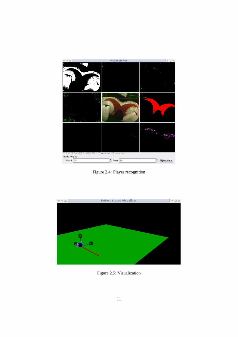
Figure 2.4: Player recognition

Figure 2.5: Visualization

11

Chapter 3

Ball Localization

3.1 Introduction

In RoboCup, estimating the position of a ball accurately is one of the most impor-tant tasks. Most robots in Middle-size League have omni-directional cameras, andin Small-size League, they use ceiling cameras to recognize objects. In the Four-legged League, however, robots have only low resolution cameras with a narrowfield of vision on their noses, while the size of the soccer field is rather large. Thesefacts make it difficult for the robots to estimate the position of the ball correctly,especially when the ball is far away or too near. Moreover, since the shutter speedof the camera is not especially fast, and its frame rate is not very high, tracking amoving object is a demanding task for the robots. In order to tackle these problems,several techniques have been proposed [22, 20]. Kalman filter method [13] is oneof the most popular techniques for estimating the position of objects in a noisy en-vironment. It is also used to track a moving ball [4]. Methods using particle filtershave been applied for tracking objects [10], and especially in Four-legged League,the method using Rao-Blackwellised particle filters has had great success[20].

In this chapter, we consider how to estimate the trajectory of the moving ball,as well as the position of the static ball, based on the Monte-Carlo localizationmethod [3]. Monte-Carlo localization has usually been used for self-localization inthe Four-legged League. We extend this to handle the localization of the ball. Wehave already mentioned a primitive method based on this idea in [11], where wehad ignored the velocity of the ball. We propose three extended methods to dealwith the velocity of the ball and report some experimental results.

3.2 Ball Recognition from the Image Data

As we have already mentioned in the previous section, the camera of the robot inFour-legged league is equipped on its nose. The field of vision is narrow (56.9◦ forhorizontal and45.2◦ for vertical), and the resolution is also low (412× 320at themaximum). Moreover, stereo vision is usually impossible, although some attempts

12

Figure 3.1: Cases of Ball Recognition. Dots on the edge show vertexes of a in-scribed triangle. The diameter of the ball is calculated by using these vertexes.

to emulate it by using plural robots have been reported [14, 26]. Therefore, first ofall, an accurate recognition of the ball from a single image captured by the camerais indispensable in estimating the position of the ball accurately. In particular, theestimation of the distance to the ball from the robot is very critical in establishinga stable method for estimating the position of the (possibly moving) ball.

A naive algorithm which counts the orange pixels in the image and uses itto estimate the distance does not work well, since the ball is often hidden by otherrobots, and the ball may be in the corner of the robot’s view as shown in Figure 3.1.In addition, the projection of the line of sight to the ground is used for calculatingthe distance to the object, but it depends on the pose of the robot and is affected bythe locomotion of the robot. In the Four-legged League, the robot’s sight is veryshaky; therefore, we do not use this method either. In this section, we will showour algorithm ability to recognize the ball and estimate the position relative to therobot from a single image. It will become the base for estimations from multipleimages, as described in the following sections.

In the image, the biggest component colored by orange and satisfying the fol-lowing heuristic conditions is recognized as the ball. (1) The edge length of thecomponent has to be more than 10 pixels, which helps exclude components toosmall. (2) The ratio of the orange pixels to the area of the bounding box must ex-ceed 40%. (3) If the component touches the edge of the image, the length of thelonger side of the bounding box must be over 20 pixels.

We use the diameter of the ball to estimate the distance to it. However, the ballis often hidden by other robots partially, and when the robot approaches to the ball,only a part of the ball is visible at the corner of the camera view. Thus the sizeof the bounding box and the total number of pixels are not enough to estimate thedistance accurately.

Figure 3.1 shows two cases of diameter estimation. When the ball is inside theview completely (left image), we regard the length of longer side of the boundingbox as the diameter of the ball. When the bounding box touches to the edges of theimage (right image), we use three points of the components, since any three pointsof the edge of a circle uniquely determine the center and the diameter of it.

13

3.3 Ball Localization using Monte-Carlo Method

In this section, we propose a technique which estimates the position and velocityof a moving ball based on the Monte-Carlo localization. This technique was intro-duced for the self-localization in [7] and utilized in [21]. The aim is to calculatethe accurate position and velocity of the ball from a series of input images. In prin-ciple, we use differences of positions between two frames. However, these datamay contain some errors. The Monte-Carlo method absorbs these errors so that theestimation of the velocity becomes more accurate. In this method, instead of de-scribing the probability density function itself, it is represented as a set ofsamplesthat are randomly drawn from it. This density representation is updated every timebased on the information from the sensors.

We consider the following three variations of the method, in order to estimateboth the position and velocity of the moving ball. (1) Each sample holds boththe position and velocity, but is updated according to only the information of theposition. (2) Each sample holds both the position and velocity, and is updatedaccording to the information of both the position and velocity. (3) Two kinds ofsamples are considered: one for the position, and the other for the velocity, whichare updated separately. For evaluating the effectiveness of our ball tracking system,we experimented in both simulated and real-world environments. The details of thealgorithms and experimental results are shown below.

3.3.1 Ball Monte-Carlo localization updated by only position infor-mation

First, we introduce a simple extension to our ball localization technique in [11]. Inthis method, a sample is a tripleai = 〈~pi ,~vi , si〉, where~pi is a position of the ball,~vi is a velocity of it, andsi is a score (1 ≤ i ≤ n) which represents how~pi and~vi fitto observations. Fig 3.2 shows the update procedure.

When the robot recognizes a ball in the image, each scoresi is updated in step6 ∼ 10, depending on the distance of~pi and the observed position~po. When theball is not found, let~po = ε. The constantτ > 0 defines theneighborhoodof thesample. Moreover, the constantsmaxupandmaxdowncontrol theconservativenessof the update. If the ratiomaxup/maxdownis small, response to the rapid change ofball’s position becomes fast, but influence of errors become strong. The thresholdvaluet controls the effect of misunderstandings. The functionrandomizeresetspi

andvi to random values andsi = 0. The functionrandom() returns a real numberrandomly chosen between 0 and 1. The return values~pe and~ve are weighted meanof samples whose scores are at leastt.

At first, we show a simulation results on this method. The simulation is per-formed as follows. We choose20 positions from(800, 1300) to (−800, 1300)atregular intervals asobserved positions, which emulates that a robot stands at thecenter of the field without any movement and watches the ball rolling from leftto right. Since in practice, the distance estimation to the ball is not very accurate

14

Algorithm BallMoteCarloLocalizationUpdatedByOnlyPositionInfor-mationInput. A set of samplesQ = {〈~pi ,~vi , si〉} and observed ball position~po

Output. estimated ball position~pe and velocity~ve.

1 for i := 1 to n do begin2 ~pi := ~pi + ~vi ;3 if ~pi is out of the fieldthen4 randomize(〈pi , vi , si〉)5 end;6 if ~po , ε then7 for i := 1 to n do begin8 score:= exp(−τ|~pi − ~po|);9 si := max(si −maxdown,min(si + maxup, score))10 end11 avgScore:= 1

n

∑ni=1 si ;

12 ~pe := ~0; ~ve := ~0; w := 0;13 for i := 1 to n do begin14 if si < avgScore· random() then15 randomize(〈pi , vi , si〉)16 else ifsi > t then begin17 ~pe := ~pe + si ~pi ;18 ~ve := ~ve + si ~vi ;19 w := w + si

20 end;21 end;22 ~pe := ~pe/w; ~ve := ~ve/w;23 output ~pe, ~ve

Figure 3.2: Procedure Ball Monte-Carlo Localization updated by only positioninformation

15

compared to the direction estimation, we added strong noise toy-direction andweak noise tox-direction of the observed positions. These positions are shown asdiamond-shaped points in Fig. 3.3 and Fig. 3.4. We examined the above methodand a simple Kalman filter method to predict the positions of the ball from thesenoisy data. The lines in Fig. 3.3 and 3.4 shows the trajectories of them for 40frames (in the first 20 frames, the observed positions are given, and in the last 20frames, no observed data is given). After some trials, we set the parameters as fol-lows. The number of samplesn = 500,maxup= 0.1, maxdown= 0.05, t = 0.15,andτ = 0.008. Compared to Kalman filter, our method failed to predict the tra-jectory of the positions after the ball is out of the view, because the velocity of thesamples did not converge well.

0

500

1000

1500

2000

2500

-1000 -500 0 500 1000 1500 2000 2500 3000

Simulated Ball PositionKalman Filter

MonteCarlo (pos only)

Figure 3.3: The result of the simulationwith Kalman filter and MonteCarlo(posonly)

0

500

1000

1500

2000

2500

-1000 -500 0 500 1000 1500 2000 2500 3000

Simulated Ball PositionMonteCarlo(pos and vel)

MonteCarlo(two sets)

Figure 3.4: The result of the simulationwith MonteCarlo(pos and vel) and Mon-teCarlo(two sets)

3.3.2 Ball Monte-Carlo localization updated by position and velocityinformation

In the previous method, each sample holds its own velocity, and in principal, goodsample holding good position and velocity would get high score. However in theprevious experiment, the velocity did not converged well. Therefore, we tried toreflect the velocity explicitly to the score, intended to accelerate the convergence.In the second method, we added the procedure shown in Fig. 3.5 to the previousmethod, between Step 10 and Step 11 in Fig. 3.2. Since theobserved velocity~vo isnot given explicitly, it is substituted by(~po− ~plast)/dt, where~plast is the last positionof the ball anddt is the difference between these two frame numbers.

The lineMonteCarlo(pos and vel)in Fig. 3.4 shows the result, with the param-etersτv = 0.08, maxupv = 1.0, maxdownv = 0.1. Unfortunately, it also failed topredict the trajectory because the converge rate was not improved well.

16

for i := 1 to n do beginscore:= exp(−τv|~vi − ~vo|);si := max(si −maxdownv,min(si + maxupv, score))

end

Figure 3.5: Additional procedure to update the score reflecting the velocity explic-itly in the second method.

3.3.3 Ball Monte-Carlo localization with two sets of samples

In the third method, we took another approach in order to reflect the goodnessof the velocity to the score. The idea is to split the samples into two categories,one for the positions〈~pi , si〉, and the other for the velocities〈~vi , si〉. The score of~p is updated in step8 ∼ 11 of PositionUpdatewhile that of~v in step2 ∼ 5 ofVelocityUpdateindependently, in Fig. 3.6.

The lineMonteCarlo(two sets)in Fig. 3.4 shows the results. The estimatedpositions fits the pathway of the rolling ball, and the predicted trajectory when ballwas out of sight is also as we expected. The effectiveness of it is comparable to theKalman filter method.

3.3.4 On the number of samples

We verified the relationship between the accuracy of the predictions and the num-ber of samples. Fig. 3.7 shows some of these experiments for the proposed threemethods. Thex-axis is the number of samples ranging10 to 1000, and they-axisis the average error of five trials, which measure the difference between the realposition and the predicted position. In the left figure, the situation was almost thesame as the previous experiments. In the right figure, we put a small obstacle infront of the robot which hides the ball in the center of the view. Because of this ob-stacle, some of observed positions were missing and the average errors increased.In general, the error decreases as the number of samples increases for all of thesethree methods. Among them, the third method which separates the samples intotwo categories performed the best. When the number of samples exceeds 150, theaccuracy did not changed in practice.

Remind that the data on observed positions, which are given as input, them-selves contained some errors. For example, the average error of the observed po-sitions was 52.6 mm in the experiment without obstacle. However, the averageerror of the third method was less than 40 mm when we took at least 150 samples,which verified that the proposed methods succeeded to stabilize the predicted ballpositions.

3.3.5 Real-world Experiments

We also performed many experiments in the real-world environments, at whichwe used the real robot in the soccer field for RoboCup competitions. We show

17

Algorithm BallMoteCarloLocalizationWithTwoSetsInput. Two sets of samplesPOS = {〈~pi , si〉} and VEL = {〈~vi , si〉}, observed ballposition~po, calculated ball velocity~vo.Output. estimated ball position~pe and velocity~ve.

PositionUpdate(POS,VEL, ~po,~vo)

1 ~ve := VelocityUpdate(VEL, ~po,~vo);2 for i := 1 to n do begin3 ~pi := ~pi + ~ve;4 if ~pi is out of the fieldthen5 randomize(〈~pi , si〉)6 end;7 if ~po , ε then8 for i := 1 to n do begin9 score:= exp(−τp|~pi − ~po|);10 si := max(si −maxdownp,

min(si + maxupp, score))11 end;12 ~pe = ~0; w = 0;13 avgScore:= 1

n

∑ni=1 si ;

14 for i := 1 to n do begin15 if si < avgScore· random() then16 randomize(〈~pi , si〉)17 else ifsi > tp then begin18 ~pe := ~pe + si ~pi ;19 w := w + si

20 end;21 end;22 ~pe := ~pe/w;23 output ~pe, ~ve

VelocityUpdate(VEL, ~po,~vo)

1 if ~po , ε then2 for i := 1 to mdo begin3 scorenew := exp(−τv|~vi − ~vo|);4 si := max(si −maxdownv,

min(si + maxupv, score))5 end;6 ~ve = ~0; w = 0;7 avgScore:= 1

m

∑mi=1 si ;

8 for i := 1 to mdo begin9 if si < avgScore· random() then10 randomize(〈~vi , si〉)11 else ifsi > tv then begin12 ~ve := ~ve + si ~vi ;13 w := w + si

14 end;15 end;16 ~ve := ~ve/w;17 output ~ve

Figure 3.6: Procedure Ball Monte-Carlo Localization with two sets of samples

18

0

200

400

600

800

1000

0 100 200 300 400 500

MonteCarlo(pos only)MonteCarlo(pos and vel)

MonteCarlo(two sets)

0

200

400

600

800

1000

0 100 200 300 400 500

MonteCarlo(pos only)MonteCarlo(pos and vel)

MonteCarlo(two sets)

Figure 3.7: Relationship between the number of samples and accuracy, in twosituations, without obstacle (left) and with an obstacle (right).

some of them in Fig. 3.8, where we compared the third method which we proposedwith the Kalman filter method. The purpose was to evaluate the robustness ofthe methods against the obstacle and the change directions of the ball movement.In the left figure, the ball rolled from right to left while a small obstacle in frontof the robot hides for some moments. In the right figure, the ball was kicked at(400,900)and went left, then it is rebounded twice at(−220,1400)and(−50,500),and disappeared from the view to the right. Mesh parts in the figures illustrates thevisible area of the robot. From these experiments, we verified that the proposedmethod is robust against the frequent change of the directions, which is often thecase in real plays.

0

500

1000

1500

2000

-600 -400 -200 0 200 400 600 800

Observed Ball PositionKalman Filter

Ball Monte-Carlo Method 0

500

1000

1500

2000

-600 -400 -200 0 200 400 600 800

Observed Ball PositionKalman Filter

Ball Monte-Carlo Method

Figure 3.8: Real world experiments. In the left situation, the ball rolled from rightto left behind a small obstacle. In the right situation, the ball started at(400,900)and rebounded twice at(−220,1400) and (−50, 500), and disappeared from theview to the right.

19

3.4 Conclusions

We proposed some applications of Monte-Carlo localization technique to track amoving ball in noisy environment, and showed some experimental results. We triedthree variations, depending on how to treat the velocity of the ball movement. Thefirst two methods did not work well as we expected, where each sample has its ownvelocity value together with the the position value. The third method, which wetreated positions and velocities separately, worked the best. We think the reasonas follows. If we treat positions and velocities together, the search space has fourdimensions. On the other hand, if we treat them separately, the search space isdivided into two spaces, each of them has two dimensions. The latter would beeasy to converge to correct values. The converge ratio is quite critical in RoboCup,because the situation changes very quickly in real games.

We compared the proposed method with Kalman filter method, which is verypopular. The experiments were not very comprehensive: for example, the observ-ing robot did not move. Nevertheless, we verified that the proposed method isattractive especially when the ball rebounds frequently in real situations.

In RoboCup domain, various techniques to improve the ball tracking abilityare proposed. For example, cooperative estimation with other robots is proposedin [5, 14]. we plan to integrate these idea into our method, and perform morecomprehensive experiments in near future.

20

Chapter 4

Learning of Ball Trapping

4.1 Introduction

For robots to function in the real world, they need the ability to adapt to unknownenvironments. These are known aslearningabilities, and they are essential in tak-ing the next step in RoboCup. As it stands now, it is humans, not the robots them-selves, that hectically attempt to adjust programs at the competition site, especiallyin the real robot leagues. But what if we look at RoboCup in a light similar to thatof the World Cup? In the World Cup, soccer players can practice and confirm cer-tain conditions on the field before each game. In making this comparison, shouldrobots also be able to adjust to new competition and environments on their own?This ability for something to learn on its own is known asautonomous learningand is regarded as important.

In this chapter, we force robots to autonomously learn the basic skills neededfor passing to each other in the four-legged robot league. Passing (including re-ceiving a passed ball) is one of the most important skills in soccer and is activelystudied in the simulation league. For several years, many studies [24, 9] have usedthe benchmark of good passing abilities, known as “keepaway soccer”, in order tolearn how a robot can best learn passing. However, it is difficult for robots to evencontrol the ball in the real robot leagues. In addition, robots in the four-leggedrobot league have neither a wide view, high-performance camera, nor laser rangefinders. As is well known, they are not made for playing soccer. Quadrupedal lo-comotion alone can be a difficult enough challenge. Therefore, they must improveupon basic skills in order to solve these difficulties, all before pass-work learningcan begin. We believe that basic skills should be learned by a real robot, becauseof the necessity of interaction with a real environment. Also, basic skills shouldbe autonomously learned because changes to an environment will always consumemuch of people’s time and energy if the robot cannot adjust on its own.

There have been many studies conducted on the autonomous learning of quadrupedallocomotion, which is the most basic skill for every movement. These studiesbegan as far back as the beginning of this research field and continue still to-

21

day [8, 15, 18, 28]. However, the skills used to control the ball are often codedby hand and have not been studied as much as gait learning. There also have beenseveral similar works related to how robots can learn the skills needed to controlthe ball. Chernova and Veloso [1] studied the learning of ball kicking skills, whichis an important skill directly related to scoring points. Zagal and Solar [29] studiedthe learning of kicking skills as well, but in a simulated environment. Althoughit was very interesting in the sense that robots could not have been damaged, thesimulator probably could not produce complete, real environments. Fidelman andStone [6] studied the learning of ball acquisition skills, which are unique to thefour-legged robot league. They presented an elegant method for autonomouslylearning these unique, advanced skills. However, there has thus far been no studythat has tried to autonomously learn the stopping and controlling of an oncom-ing ball, i.e. trapping the ball. In this paper, we present an autonomous learningmethod for ball trapping skills. Our method will enhance the game by way oflearned pass-work in the four-legged robot league.

4.2 Preliminary

4.2.1 Ball Trapping

Before any learning can begin, we first have to accurately create the appropriatephysical motions to be used in trapping a ball accurately before the learning pro-cess. The picture in Fig. 4.1 (a) shows the robot’s pose at the end of the motion.The robot begins by spreading out its front legs to form a wide area with which toreceive the ball. Then, the robot moves its body back a bit in order to absorb theimpact caused by the collision of the body with the ball and to reduce the reboundspeed. Finally, the robot lowers its head and neck, assuming that the ball has passedbelow the chin, in order to keep the ball from bouncing off of its chest and awayfrom its control. Since the camera of the robot is equipped on the tip of the nose,it actually cannot watch the ball below the chin. This series of motions is treatedas single motion, so we can neither change the speed of the motion, nor interruptit, once it starts. It takes 300 ms (= 60 steps× 5 ms) to perform. As opposed tograbbing or grasping the ball, this trapping motion is instead thought of as keepingthe ball, similar to how a human player would keep control of the ball under his/herfoot.

The judgment of whether the trap succeeded or failed is critical for autonomouslearning. Since the ball is invisible to the robot’s camera when it’s close to therobot’s body, we utilized the chest PSD sensor. However, the robot cannot make anaccurate judgment when the ball is not directly in front of their chest or after it takesa droopy posture. Therefore, we utilized a “pre-judgment motion”, which takes 50ms (= 10 steps× 5 ms), immediately after the trapping motion is completed, asshown in Fig. 4.1 (b). In this motion, the robot fixes the ball between its chin andchest and then lifts its body up slightly so that the ball will be located immediatelyin front of the chest PSD sensor, assuming the ball was correctly trapped to begin

22

(a) trapping motion (b) pre-judgment motion

Figure 4.1: The motion to actually trap the ball (a), and the motion to judge if itsucceeded in trapping the ball (b).

with.

4.2.2 One-dimensional Model of Ball Trapping

Acquiring ball trapping skills in solitude is usually difficult, because robots must beable to search for a ball that has bounced off of them and away, then move the ballto an initial position, and finally kick the ball again. This requires sophisticated,low-level programs, such as an accurate, self-localization system; a strong shot thatis as straight as possible; and a locomotion which utilizes the odometer correctly.In order to avoid additional complications, we simplify the learning process a bitmore.

First, we assume that the passer and the receiver face each other when thepasser passes the ball to the receiver, as shown Fig. 4.2. The receiver tries to facethe passer while watching the ball that the passer is holding. At the same time, thepasser tries to face the receiver while looking at the red or blue chest uniform ofthe receiver. This is not particularly hard to do, and any team should be able toaccomplish it. As a result, the robots will face each other in a nearly straight line.The passer need only shoot the ball forward so that the ball can go to the receiver’schest. The receiver, in turn, has only to learn a technique for trapping the oncomingball without it bouncing away from its body.

Ideally, we would like to treat our problem, which is to learn ball trappingskills, one-dimensionally. In actuality though, the problem cannot be fully viewedin one-dimension, because either the robots might not precisely face each other ina straight line, or because the ball might curve a little due to the grain of the grass.We will discuss this problem in Section 4.7.

23

Figure 4.2: One-dimensional model of ball trapping problem.

Figure 4.3: Training equipment for learning ball trapping skills.

4.3 Training Equipment

The equipment we prepared for learning ball trapping skills in one-dimensionalis fairly simple. As shown in Fig. 4.3, the equipment has rails of width nearlyequal to an AIBO’s shoulder-width. These rails are made of thin rope or string,and their purpose is to restrict the movement of the ball, as well as the quadrupedallocomotion of the robot, to one-dimension. Aside from these rails, the robots usea slope placed at the edge of the rail when learning in solitude. They kick the balltoward the slope, and they can learn trapping skills by trying to trap the ball afterit returns from having ascended the slope.

4.4 Learning Method

Fidelman and Stone [6] showed that the robot can learn to grasp a ball. They em-ployed three algorithms: hill climbing, policy gradient, and amoeba. We cannot,however, directly apply these algorithms to our own problem because the ball ismoving fast in our case. It may be necessary for us to set up an equation which

24

incorporates the friction of the rolling ball and the time at which the trapping mo-tion occurs if we want to view our problem in a manner similar to these para-metric learning algorithms. In this chapter, we apply reinforcement learning algo-rithms [27]. Since reinforcement learning requires no background knowledge, allwe need to do is give the robots the appropriate reward for a successful trapping sothat they can successfully learn these skills.

The reinforcement learning process is described as a sequence of states, ac-tions, and rewards

s0,a0, r1, s1,a1, r2, . . . , si ,ai , r i+1, si+1, ai+1, r i+2, . . . ,

which is a reflection of the interaction between the learner and the environment.Here,st ∈ S is a state given from the environment to the learner at timet (t ≥ 0),andat ∈ A(st) is an action taken by the learner for the statest, whereA(st) isthe set of actions available in statest. One time step later, the learner receives anumerical rewardrt+1 ∈ R, in part as a consequence of its action, and finds itself ina new statest+1.

Our interval for decision making is 40 ms and is in synchronization with theframe rate of the CCD-camera. In the sequence, we treat each 40 ms as a singletime step, i.e.t = 0, 1,2, · · · means 0 ms, 40 ms, 80 ms,· · · , respectively. In ourexperiments, the states essentially consist of the information on the moving ball:relative position to the robot, moving direction, and the speed, which are estimatedby our vision system. Since we have restricted the problem to one-dimensionalmovement in Section 4.2.2, the state can be represented by a pair of scalar variablesx anddx. The variablex refers to the distance from the robot to the ball estimatedby our vision system, anddx simply refers to the difference between the currentx and the previousx of one time step before. We limited the range of these statevariables such thatx is in [ 0 mm, 2000 mm ], anddx in [ −200mm, 200 mm ].This is because if a value ofx is greater than 2000, it will be unreliable, and if theabsolute value ofdx is greater than 200, it must be invalid in games (e.g.dxof 200mm means 5000 mm/s).

Although the robots have to do a large variety of actions to perform fully-autonomous learning by nature, as far as our learning method is concerned, we canfocus on the following two macro-actions. One istrap, which initiates the trappingmotions described in Section 4.2.1. The robot’s motion cannot be interrupted for350 ms until the trapping motion finishes. The other isready, which moves its headto watch the ball and preparing totrap. Each reward given to the robot is simplyone of{+1,0,−1}, depending on whether it successfully traps the ball or not. Therobot can make a judgment of that success by itself using its chest PSD sensor. Thereward is1 if the trap action succeeded, meaning the ball was correctly capturedbetween the chin and the chest after thetrap action. A reward of−1 is given eitherif the trap action failed, or if the ball touches the PSD sensor before thetrap actionis performed. Otherwise, the reward is0. We define the period from kicking theball to receiving any reward other than 0 as oneepisode. For example, if the current

25

episode ends and the robot moves to a random position with the ball, then the nextepisode begins when the robot kicks the ball forward.

In summary, the concrete objective for the learner is to acquire the correcttiming for when to initiate the trapping motion depending on the speed of theball by trial and error. Fig. 4.4 shows the autonomous learning algorithm usedin our research. It is a combination of the episodic SMDP Sarsa(λ) with the lin-ear tile-coding function approximation (also known as CMAC). This is one of themost popular reinforcement learning algorithms, as seen by its use in the keepawaylearner [24].

Here,Fa is a feature setspecified by tile coding with each actiona. In thispaper, we use two-dimensional tiling and set the number of tilings to 32 and thenumber of tiles to about 5000. We also set the tile width ofx to 20 and the tilewidth of dx to 50. The vector

−→θ is a primary memory vector, also known as a

learning weight vector, andQa is aQ-value, which is represented by the sum of−→θ

for each value ofFa. The policyε-greedyselects a random action with probabilityε, and otherwise, it selects the action with the maximumQ-value. We setε = 0.01.Moreover,−→e is aneligibility trace, which stores the credit that past action choicesshould receive for current rewards.λ is a trace-decay parameterfor the eligibilitytrace, and we simply setλ = 0.0. We set thelearning rate parameterα = 0.5 andthediscount rate parameterγ = 1.0.

4.5 Experiments

4.5.1 Training Using One Robot

We first experimented by using one robot along with the training equipment thatwas illustrated in Section 4.3. The robot could train in solitude and learn balltrapping skills on its own.

Fig. 4.5(a) shows the trapping success rate, which is how many times the robotsuccessfully trapped the ball in 10 episodes. It reached about 80% or more after 250episodes, which took about 60 minutes using 2 batteries. Even if robots continue tolearn, the success rate is unlikely to ever reach 100%. This is because the trappingmotions, which force the robot to move slightly backwards in order to try andreduce the bounce effect, can hardly be expected to capture a slow, oncoming ballthat stops just in front of it.

Fig. 4.6 shows the result of each episode by plotting a circle if it was successful,a cross if it failed in spite of trying to trap, and a triangle if it failed because of doingnothing. From the 1st episode to the 50th episode, the robots simply tried to trapthe ball while it was moving with various velocities and at various distances. Theymade the mistake of trying to trap the ball even when it was moving away (dx> 0),because we did not give them any background knowledge, and we only gave them

26

while still not acquiring trapping skillsdo1

go get the ball and move to a random position with the ball;2

kick the ball toward the slope;3

s← a state observed in the real environment;4

forall a ∈ A(s) do5

Fa← set of tiles fora, s;6

Qa← ∑i∈Fa

θ(i);7

end8

lastAction← an optimal action selected byε-greedy;9−→e ← 0;10

forall i ∈ FlastActiondo e(i)← 1;11

reward← 0;12

while reward= 0 do13

do lastAction;14

if lastAction= trap then15

if the ball is heldthen reward← 1;16

else reward← −1;17

else18

if collision occursthen reward← −1;19

else reward← 0;20

end21

δ← reward− QlastAction;22

s← a state observed in the real environment;23

forall a ∈ A(s) do24

Fa← set of tiles fora, s;25

Qa← ∑i∈Fa

θ(i);26

end27

lastAction← an optimal action selected byε-greedy;28

δ← δ + QlastAction;29−→θ ← −→θ + αδ−→e;30

QlastAction← ∑i∈FlastAction

θ(i);31−→e ← λ−→e;32

if player acting in states then33

forall a ∈ A(s) s.t. a , lastActiondo34

forall i ∈ Fa do e(i)← 0;35

end36

forall i ∈ FlastActiondo e(i)← 1;37

end38

end39

δ← reward− QlastAction;40−→θ ← −→θ + αδ−→e;41

end42

Figure 4.4: Algorithm of our autonomous learning (based on keepawaylearner [24]).

27

0 50 100 150 200 250 300 350

episodes

0

20

40

60

80

100

trappin

g s

uccess r

ate

(a) one robot

0 50 100 150 200 250 300 350

episodes

0

20

40

60

80

100

trappin

g s

uccess r

ate

ALPL

(b) two robots

0 50 100 150 200 250 300 350 400

episodes

0

20

40

60

80

100

trappin

g s

uccess r

ate

ALPL

(c) two robots with communication

Figure 4.5: Results of three experiments.

28

0 500 1000 1500 2000

x

-200

-150

-100

-50

0

50

100

150

200

dx

failuresuccesscollision

(a) Episodes 1–50

0 500 1000 1500 2000

x

-200

-150

-100

-50

0

50

100

150

200

dx

failuresuccesscollision

(b) Episodes 51–100

0 500 1000 1500 2000

x

-200

-150

-100

-50

0

50

100

150

200

dx

failuresuccesscollision

(c) Episodes 101–150

0 500 1000 1500 2000

x

-200

-150

-100

-50

0

50

100

150

200

dx

failuresuccesscollision

(d) Episodes 151–200

Figure 4.6: Learning process from 1st episode to 200th episode. A circle indi-cates successful trapping, a cross indicates failed trapping, and a triangle indicatescollision with the ball.

two variables:x anddx. From the 51st episode to the 100th episode, they learnedthat they could not trap the ball when it was far away (x > 450) or when it wasmoving away (dx > 0). From the 101st episode to 150th episode, they began tolearn the correct timing for a successful trapping, and from the 151st episode to200th episode, they almost completely learned the correct timing.

4.5.2 Training Using Two Robots

In the case of training using two robots, we simply replace the slope in the trainingequipment with another robot. We call the original robot theActive Learner(AL)and the one which replaced with slope thePassive Learner(PL). AL is the same asin case of training using one robot. On the other hand, PL differs from AL in thatPL does not search out nor approach the ball if the trapping failed. Only AL does

29

0 20 40 60 80 100 120 140

time step

-500

0

500

1000

1500

2000

x /

dx

xdx

Figure 4.7: The left figure shows how our vision system recognizes a ball whenthe other robot holds it. The ball looks to be smaller than it is, because a part ofit is hidden by the partner and its shadow, resulting in an estimated distance tothe ball that is further away than it really is. The right figure plots the estimatedvalues of the both the distancex and the velocitydx, when the robot kicked theball to its partner, the partner trapped it, and then the partner kicked it back. Whenthe training partner was holding the ball under its head though (the center of thegraph), we can see the robot obviously miscalculated ball’s true distance.

so. Other than this difference, PL and AL are basically the same.We experimented for 60 minutes by using both AL and PL that had learned

in solitude for 60 minutes using the training equipment. Theoretically, we wouldexpect them to succeed in trapping the ball after only a short time. However, bytrying to trap the ball while in obviously incorrect states, they actually failed re-peatedly. The reason for this was because the estimation of the ball’s distance tothe robot-in-waiting became unreliable, as shown in Fig. 4.7. This, in turn, wasdue to the other robot holding the ball below its head before kicking it forward toits partner. Such problems can occur during the actual games, especially in poorlighting conditions, when teammates and adversaries are holding the ball.

Although we are of course eager to overcome this problem, we should notforce a solution that discourages the robots from holding the ball first, because ballholding skills help them to properly judge whether or not they can successfullytrap the ball. It also serves another purpose, which is to give the robots a nicer,straighter kick. Moreover, there is no way we can absolutely keep the adversaryrobots from holding the ball. Although there are several solutions (e.g. measuringthe distance to the ball by using green pixels or sending the training partner to getthe ball), we simply continued to make the robots learn without having made anychanges. This was done in an attempt to allow the robots to gain experience relatedto irrelevant states. In fact, it turns out they should never try to trap the ball whenx ≥ 1000anddx ≥ 200. Moreover, they should probably not try to trap the ballwhenx ≥ 1000anddx≤ −200.

30

Fig. 4.5(b) shows the results of training using two robots. They began to learnthat they should probably not try to trap the ball while in irrelevant states, as thiswas a likely indicator that the training partner was in possession of the ball. Thiswas learned quite slowly though, because the AL can only learn successful trappingskills when PL itself succeeds. If PL fails, AL’s episode is not incremented. Evenif the player nearest the ball can go get it, the problem is not resolved because thenthey just learn slowly in the end, though simultaneously.

4.5.3 Training Using Two Robots with Communication

Training using two robots, like in the previous section, unfortunately takes a longtime to complete. In this section, we will look at accelerating their learning byallowing them to communicate with each other.

First, we made the robots share their experiences with each other, as in [19].However, if they continuously communicated with each other, they could not doanything else, because the excessive processing would interrupt the input of properstates from the real-time environment. Therefore, we made the robots exchangetheir experiences, which included what actionat they performed, the values of thestate variablesxt anddxt, and the rewardrt+1 at timet, but this was done only whenthey received a reward other than 0, i.e. the end of each episode. They then updated

their−→θ values using the experiences they received from their partner. As far as the

learning achievements for our research is concerned, they can successfully learnenough using this method.

We also experimented in the same manner as Section 4.5.2 using two robotswhich can communicate with each other. Fig. 4.5(c) shows the results of this ex-periment. They could rapidly adapt to unforeseen problems and acquire practicaltrapping skills. Since PL learned its skills before AL learned, it could relay to ALthe helpful experience, effectively giving AL about a 50% learned status from thebeginning. These results indicate that the robots with communication learned morequickly than the robots without communication.

4.6 Discussion

The three experiments above showed that robots could efficiently learn ball trap-ping skills and that the goal of pass-work by robots can be achieved in one-dimension.In order to briefly compare those experiments, Fig. 4.8 presents a few graphs,where thex-axis is the elapsed time and they-axis is the total number of successesso far. Fig. 4.8(a) and Fig. 4.8(b) shows the learning process with and withoutcommunication, respectively, for 60 minutes after pre-learning for 60 minutes byusing two robots from the beginning. Fig. 4.8(c) and Fig. 4.8(d) shows the learningprocess with and without communication, respectively, after pre-learning for 60minutes in solitude.

Comparing (a) and (c) with (b) and (d) has us conclude that allowing AL and

31

0 10 20 30 40 50 60

minutes

0

20

40

60

80

100

120

140

tota

l num

ber

of

successfu

l tr

appin

g

ALPL

(a) without communication after pre-learning by using two robots

0 10 20 30 40 50 60

minutes

0

20

40

60

80

100

120

140

tota

l num

ber

of

successfu

l tr

appin

g

ALPL

(b) with communication after pre-learningby using two robots

0 10 20 30 40 50 60

minutes

0

20

40

60

80

100

120

140

tota

l num

ber

of

successfu

l tr

appin

g

ALPL

(c) without communication after pre-learning in solitude

0 10 20 30 40 50 60

minutes

0

20

40

60

80

100

120

140

tota

l num

ber

of

successfu

l tr

appin

g

ALPL

(d) with communication after pre-learningin solitude

Figure 4.8: Total numbers of successful trappings with respect to the elapsed time.

PL to communicate with each other will lead to more rapid learning compared tono communication. Comparing (a) and (b) with (c) and (d), the result is differentfrom our expectation. Actually, the untrained robots learned as much as or betterthan trained robots for 60 minutes. The trained robots seems to be over-fitted forslow-moving balls, because the ball was slower in the case of one robot learningthan in the case of two due to friction on the slope. However, it is still good strategyto train robots in solitude at the beginning, because experiments that solely use tworobots can make things more complicated. In addition robots should also learn theskills for a relatively slow-moving ball anyway.

32

4.7 Conclusions and Future Work

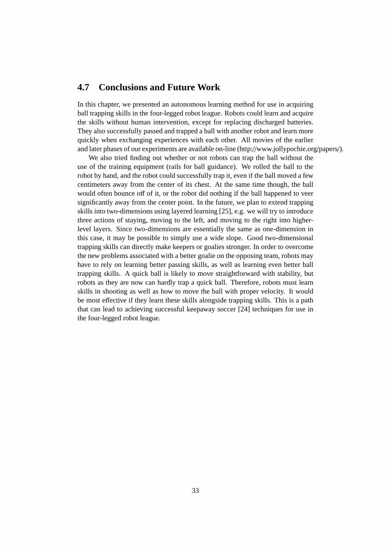
In this chapter, we presented an autonomous learning method for use in acquiringball trapping skills in the four-legged robot league. Robots could learn and acquirethe skills without human intervention, except for replacing discharged batteries.They also successfully passed and trapped a ball with another robot and learn morequickly when exchanging experiences with each other. All movies of the earlierand later phases of our experiments are available on-line (http://www.jollypochie.org/papers/).

We also tried finding out whether or not robots can trap the ball without theuse of the training equipment (rails for ball guidance). We rolled the ball to therobot by hand, and the robot could successfully trap it, even if the ball moved a fewcentimeters away from the center of its chest. At the same time though, the ballwould often bounce off of it, or the robot did nothing if the ball happened to veersignificantly away from the center point. In the future, we plan to extend trappingskills into two-dimensions using layered learning [25], e.g. we will try to introducethree actions of staying, moving to the left, and moving to the right into higher-level layers. Since two-dimensions are essentially the same as one-dimension inthis case, it may be possible to simply use a wide slope. Good two-dimensionaltrapping skills can directly make keepers or goalies stronger. In order to overcomethe new problems associated with a better goalie on the opposing team, robots mayhave to rely on learning better passing skills, as well as learning even better balltrapping skills. A quick ball is likely to move straightforward with stability, butrobots as they are now can hardly trap a quick ball. Therefore, robots must learnskills in shooting as well as how to move the ball with proper velocity. It wouldbe most effective if they learn these skills alongside trapping skills. This is a paththat can lead to achieving successful keepaway soccer [24] techniques for use inthe four-legged robot league.

33

Chapter 5

Strategy System

This year, we changed the description method of our high-level strategies to a sim-ple if-then rule method from a state transition method. The state transition methodallows us to quickly develop step-by-step actions, e.g., actions which perform a cer-tain action after achieving another certain action. This method, however, results inannoying debugging work when we create huge programs, because we must care-fully make sure that all transitions in all states are valid (otherwise, robots may stopmoving because of an infinite loop transition or a transition to an unknown state).On the other hand, the if-then rule method allows us to create readable and briefprogram codes which we can debug easily, although we must write more complexprogram codes for such step-by-step actions. We intend to utilize machine learningtechniques for acquiring more complex rules as sophisticated strategies next year.

We also changed our behavior system, by which our low-level strategies werecreated, for new high-level strategies. Our behavior system still supports the statetransition method, because low-level strategies mostly include step-by-step actions.

5.1 Behavior System

The new behavior system is based on our behavior system of last year. The differ-ence from the old one is to utilize two types of behaviors. One is a normal behav-ior, and the other is a non-stop behavior. The normal behaviors can be exchangedanytime, while the non-stop behaviors can never be exchanged until they are ter-minated. For example, the normal behaviors include approaching, positioning,dribbling, and so on; The non-stop behaviors include shooting, guarding, catching,and so on, which must be continued even if the situation is changed (e.g., the ballis lost) during executing the behaviors.

The following code is an example of behavior creation in our system. The func-tion “init” is called only once at the beginning. The function “setState” changesthe behavior’s state, which is also a function name that called by the system everydecision-making time. This example prints the string “action01” only once, i.e.the function “init”, “action01”, “finish”, “finish”, ... are called during executing

34

the behavior “foo”, in that order.

foo = Behavior("foo") -- or NonstopBehavior("foo")

function foo.init()foo.setState("action01")

end

function foo.action01()print("action01")foo.setState("finish")

end

function foo.finish()end

Moreover, we established a combo behavior mechanism that can combine sev-eral behaviors. For example, we can create a behavior shooting a ball after catchingit by combining a shooting behavior and a catching behavior. The following codeis an example of combining two behaviors. The combo behavior “comboFooBar”means the behavior “bar” is executed right after the behavior “foo” is terminated.

foo = Behavior("foo")...bar = Behavior("bar")...comboFooBar = ComboBehavior(foo, bar)

35

Chapter 6

Strategies for Jolly Pochie 2006

6.1 Attacker

This year, we used two types of attacker scripts. One is “AtFG” we call. It designedfor games. The other is “AtMAX”. It designed for the penalty shoot-out and the newgoal challenge. The difference between these two scripts is the way of shootingand approaching. Our attacker has some various shots in games. It chooses one ofthem depending on the situation. However it shoots only one way in the penaltyshoot-out. The shoot is very strong and carries the ball far. In addition the playerapproaches the ball more carefully in penalty shoot-out than in games. In penaltyshoot-out, this is because the attacker needs to catch the ball more surely.

Our attacker was designed with if-then rule. Last year it was designed basedon a state transition method. This method, however, often causes bugs in scriptcodes. This year our goalie script was written with a if-then rule method. Theif-then rule is very simple and has less incidence of bugs. We describe these detailsin the following sections.

The attacker has the following five processes. We named them as “search”,“approach”, “ shoot”, “ support”, and “localize”. Each of them is used dependingon the situation.

6.1.1 Search

The attacker searches the ball in the “search” process. When the attacker can notsee the ball, the “search” process is called to find the ball. This process consists ofthe following behaviors.

• “SearchWalk”: The attacker searches the ball with walking from one side ofthe field to the other.

• “SearchDown”: The attacker searches the ball under its head by swinging itshead.

• “SearchTurn”: The attacker searches the ball with turning right or left.

36

We improved the method of searching the ball. When the attacker lost the ball,it looked near and far at first in the last year. If it was not able to find the balleven though this process had been over, it turned to the rotative direction where theattacker had seen the ball last time. This year the attacker turned after swinging itsown head only once.

6.1.2 Approach

The attacker approaches the ball enough to shoot or catch it in the “approach”process. When it watches the ball, the “approach” process is called.

6.1.3 Shoot

The attacker tries to score in the “shoot” process. When the attacker is near the ballenough to shoot or catch it, this process is called.

If the attacker can catch it easily, it tries to do. After catching it, the attackerturns to the direction of the opponent goal. If it can see the opponent goal or theregulation time for continuous catching is over, the attacker shoots it.

If the attacker can not catch easily, it tries to shoot it. The attacker has variousshots, and it chooses the best shot for scoring.

6.1.4 Support

We built a communication system for supporting the other teammates. The systemallows the players to communicate with each other. They can tell each other someinformation: their own position, the relative ball position, and the sending time.

We developed two strategies, “active” and “passive”, and made our attackersswitch their strategy. In case that any other teammate is not chasing the ball, theattacker plays with the “active” strategy. It allows the attacker to use the “search”,“approach” and “shoot” processes. Otherwise, that is, in case that other teammateis the nearest to the ball and chasing it, the attacker plays with the “passive” strat-egy. It allows the attacker to use only the “search” and “support” processes. Theattacker can not call the “approach” process so that it does not clash with otherteammates. This strategy system allows only one attacker to approach the ball.However our defender and goalie do not use the system. This is because they mustclear the ball even if they have the risk of clashing other teammates.

When the “support” process is called, the attacker does not approach andmoves to a supporting position which is between the ball and the opponent goal.The attacker stays in the supporting position until other player moves the ball.

6.1.5 Localize

This year, our attacker is always localizing own position in games, because stop-ping for the localization wastes its playing time. However, some clashes still oftenbring the attacker misunderstanding of its own position localization, and it can not

37

estimate its own position correctly when it is in the “penalty” state. In that case, the“ localize” process is called expressly. When it is called, the attacker stops walkingand estimates its own position by looking around carefully.

6.1.6 Problems for next year

We have the following problems that we try to solve next year.

The accuracy of catching and shooting

This year, when the player found the ball, the player approached, caught, and shotit. However, the player often failed to catch the ball, and was not able to shoot it inimportant occasions. Therefore, we need to improve the catching motion and theshooting motion. As a strategy, we need to adjust the condition of switching the“shoot” process and the “approach” process.

The avoidance of the penalties of illegal defender

As to illegal defender, we designed the script so that the defender should not enterthe own penalty area. However, we did not designed this script for the attacker,because we had thought that the attacker rarely entered in its own penalty area.As a result, the attacker often entered the own penalty area and was received thepenalty. Therefore, we need to apply this script to the attacker next year.

The improvement of supporting each other

We need to improve the supporting system. This year, the player switched the“active” and “passive” strategies depending on the distance of the ball. In the“passive” strategy, the player only stays in the place. Therefore, the player needsto do more sophisticated action, e.g., it continues to move dynamically to turn anysituation to its advantage.

6.2 Defender

The strategy of our defender is almost the same as that of the attacker. However,the defender should be more defensive than attackers. We devised the strategy ofthe defender. The detail is as follows.

First, the defender does not go out over a half line. Second, when the ballis an opposite side, the defender stays at its own position. Third, when the ballcomes into the defender’s face, either the “guard" or the “clear" process is calleddepending on the situation.

38

Figure 6.1: The strategy of Attacker

6.3 Goalie

Our goalie’s strategy is separated into four processes: “search”, “ position”, “ guard”,and “clear”. First, our goalie is positioned at the center of its own goal in the “po-sition” process, because it is the most important for the goalie to be in front of itsown goal. Second, the “search” process is called, if the goalie does not see theball. The goalie must recognize the current position of the ball to respond to themovement of it. Next, the goalie saves in the “guard” process. An opponent wouldshoot the ball at the chink of the goal. Therefore, the goalie can not defend its owngoal only by standing in front of our goal. The goalie must move left or right tofill up the chink and defend its own goal by opening the legs. Finally, the goalieapproaches the ball and kicks it out in the “clear” process. In case there is the ballinside the penalty area, the goalie must clear it courageously. This year the “guard”and “clear” processes are especially improved . Each process is described in detailin the following.

6.3.1 Position

The “position” process (cf. Fig. 6.2a) is the most important for the goalie. If thegoalie is not in front of its own goal at a crucial moment (e.g. when an opponentshoots the ball to our goal), it will be equal to giving an opposing team one point.

39

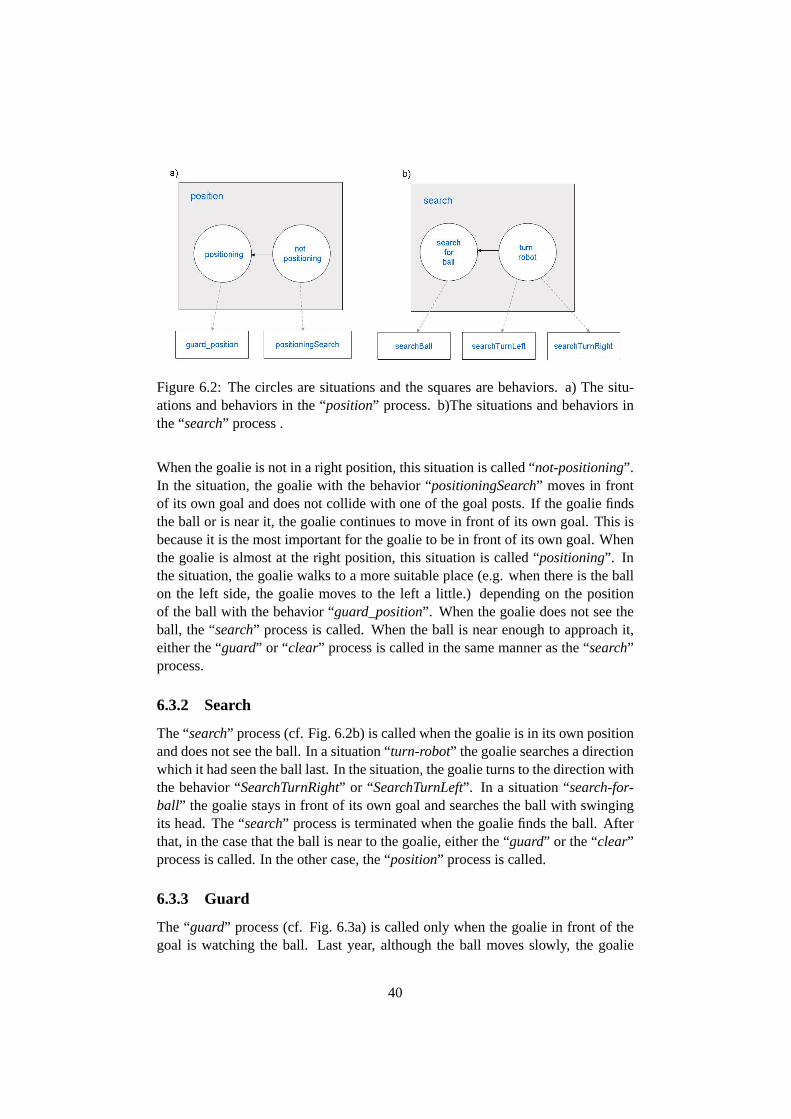
Figure 6.2: The circles are situations and the squares are behaviors. a) The situ-ations and behaviors in the “position” process. b)The situations and behaviors inthe “search” process .

When the goalie is not in a right position, this situation is called “not-positioning”.In the situation, the goalie with the behavior “positioningSearch” moves in frontof its own goal and does not collide with one of the goal posts. If the goalie findsthe ball or is near it, the goalie continues to move in front of its own goal. This isbecause it is the most important for the goalie to be in front of its own goal. Whenthe goalie is almost at the right position, this situation is called “positioning”. Inthe situation, the goalie walks to a more suitable place (e.g. when there is the ballon the left side, the goalie moves to the left a little.) depending on the positionof the ball with the behavior “guard_position”. When the goalie does not see theball, the “search” process is called. When the ball is near enough to approach it,either the “guard” or “ clear” process is called in the same manner as the “search”process.

6.3.2 Search

The “search” process (cf. Fig. 6.2b) is called when the goalie is in its own positionand does not see the ball. In a situation “turn-robot” the goalie searches a directionwhich it had seen the ball last. In the situation, the goalie turns to the direction withthe behavior “SearchTurnRight” or “ SearchTurnLeft”. In a situation “search-for-ball” the goalie stays in front of its own goal and searches the ball with swingingits head. The “search” process is terminated when the goalie finds the ball. Afterthat, in the case that the ball is near to the goalie, either the “guard” or the “clear”process is called. In the other case, the “position” process is called.

6.3.3 Guard

The “guard” process (cf. Fig. 6.3a) is called only when the goalie in front of thegoal is watching the ball. Last year, although the ball moves slowly, the goalie

40

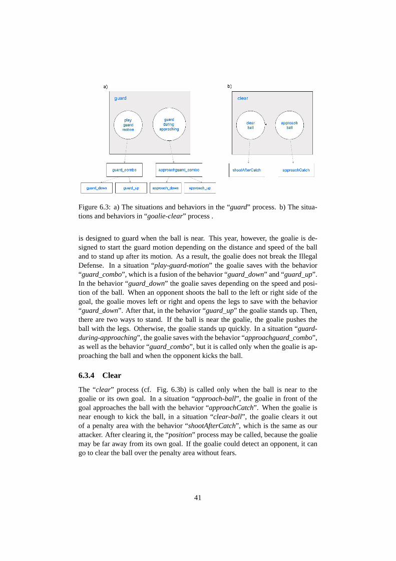
Figure 6.3: a) The situations and behaviors in the “guard” process. b) The situa-tions and behaviors in “goalie-clear” process .

is designed to guard when the ball is near. This year, however, the goalie is de-signed to start the guard motion depending on the distance and speed of the balland to stand up after its motion. As a result, the goalie does not break the IllegalDefense. In a situation “play-guard-motion” the goalie saves with the behavior“guard_combo”, which is a fusion of the behavior “guard_down” and “guard_up”.In the behavior “guard_down” the goalie saves depending on the speed and posi-tion of the ball. When an opponent shoots the ball to the left or right side of thegoal, the goalie moves left or right and opens the legs to save with the behavior“guard_down”. After that, in the behavior “guard_up” the goalie stands up. Then,there are two ways to stand. If the ball is near the goalie, the goalie pushes theball with the legs. Otherwise, the goalie stands up quickly. In a situation “guard-during-approaching”, the goalie saves with the behavior “approachguard_combo”,as well as the behavior “guard_combo”, but it is called only when the goalie is ap-proaching the ball and when the opponent kicks the ball.

6.3.4 Clear

The “clear” process (cf. Fig. 6.3b) is called only when the ball is near to thegoalie or its own goal. In a situation “approach-ball”, the goalie in front of thegoal approaches the ball with the behavior “approachCatch”. When the goalie isnear enough to kick the ball, in a situation “clear-ball”, the goalie clears it outof a penalty area with the behavior “shootAfterCatch”, which is the same as ourattacker. After clearing it, the “position” process may be called, because the goaliemay be far away from its own goal. If the goalie could detect an opponent, it cango to clear the ball over the penalty area without fears.

41

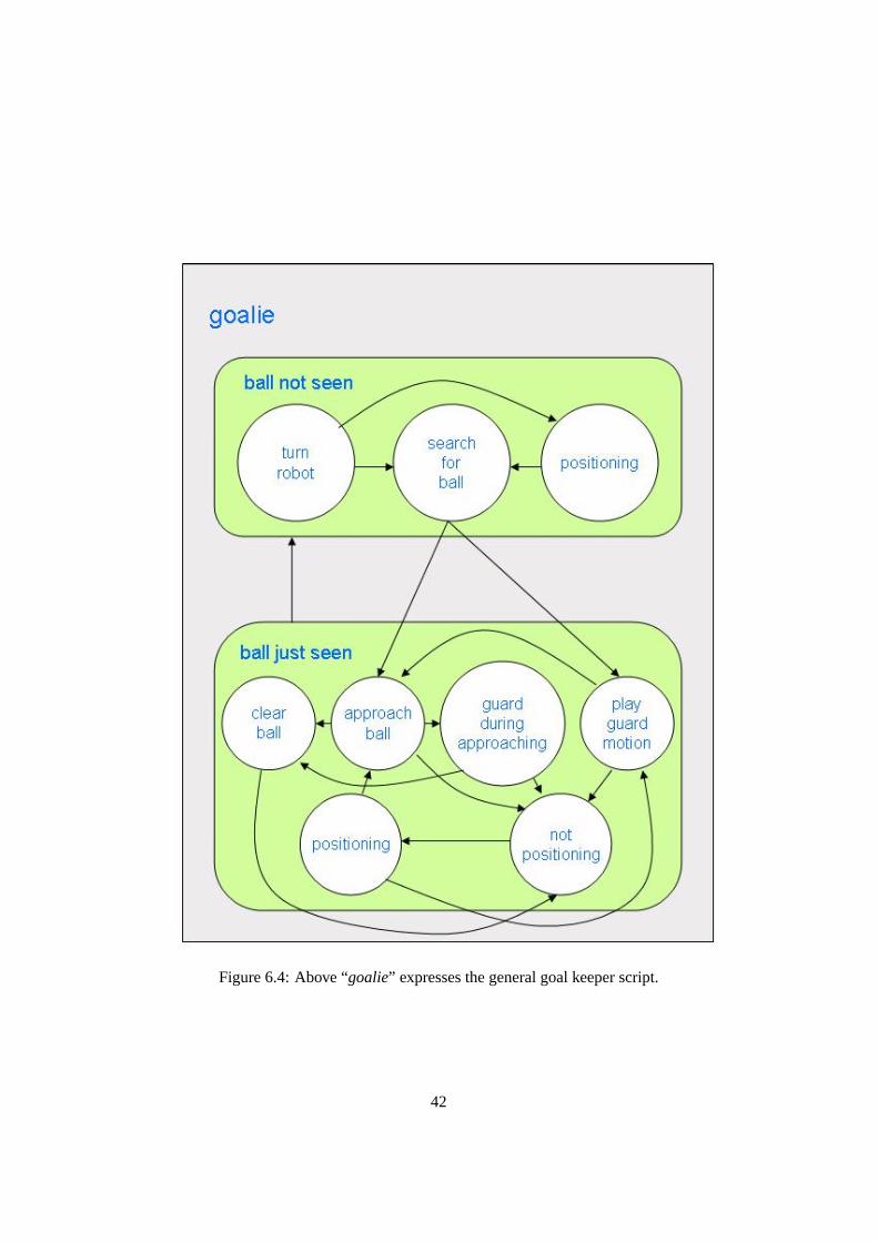
Figure 6.4: Above “goalie” expresses the general goal keeper script.

42

6.3.5 Conclusion

The goalie’s script is such as Fig. 6.4. In the “goalie”, all the processes (“position”,“search”, “ guard”, and “clear”) are included. It is possible to divide them into twogroups. One group is “ball-not-seen” which consists of situations which the goaliedoes not see the ball. The other is “just-ball-seen” which consists of situationswhich the goalie sees the ball. In the former, if the goalie is in front of the goal andits situation is “search-for-ball”, the goalie tries to find the ball with the behavior“searchBall”. When the goalie finds the ball, its situation changes to the situation“approach-ball” or “ play-guard-motion”. In the latter, all the processes exceptprocess “search” are called depending on the position, the speed of the ball, and soon. When the goalie does not see the ball, the situation of the goalie is changed tothe group “ball-not-seen” at once.

6.3.6 Problems for Next Year

We must improve our positioning skills. For instance, there is a possibility that thegoalie loses its own position by colliding with the edges of its own goal. In order toavoid this trouble, we need to develop a collision detection system by monitoringits joint angles, our positioning system to avoid colliding with the edges, a morerobust localization system, and so on. In the “position” process, the goalie is inthe center of the goal this year. However, we hope that the goalie is designed toposition with the information of the ball. For example, the goalie walks a few stepsto the side the ball is in, because the goalie more effectively fills up a chink of thegoal and saves. In the “search” process, the ball sometimes is in a blind spot of thegoalie, nevertheless it is in front of its own goal. For example, it is possible that theball is at the back of the goalie. The nearer to the goal the goalie is, the smaller theblind spot in front of the goal is. Therefore, the behavior is needed to let the goaliestep back to its own goal while searching for the ball. The “guard” process needsto estimate the speed and direction of the ball more robust. In the “clear” process,when the ball is between the goalie and its own goal, it is necessary that the goaliemust not shoot toward its own goal but clear the ball out of the penalty area.

43

Chapter 7

Shot Motions

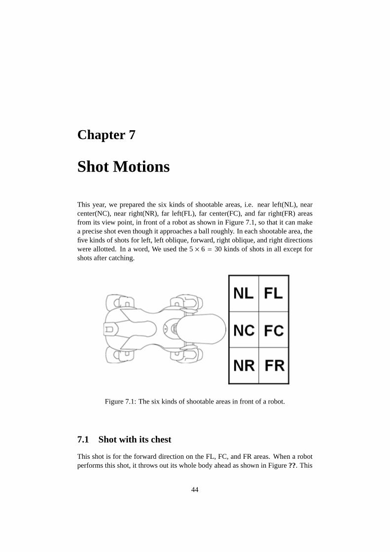
This year, we prepared the six kinds of shootable areas, i.e. near left(NL), nearcenter(NC), near right(NR), far left(FL), far center(FC), and far right(FR) areasfrom its view point, in front of a robot as shown in Figure 7.1, so that it can makea precise shot even though it approaches a ball roughly. In each shootable area, thefive kinds of shots for left, left oblique, forward, right oblique, and right directionswere allotted. In a word, We used the5 × 6 = 30 kinds of shots in all except forshots after catching.

Figure 7.1: The six kinds of shootable areas in front of a robot.

7.1 Shot with its chest

This shot is for the forward direction on the FL, FC, and FR areas. When a robotperforms this shot, it throws out its whole body ahead as shown in Figure??. This

44

shot has the advantage of high hitting ratio by using large area of its chest. How-ever, this shot also has the disadvantage of a concentrated load for servo motors ofits front legs, because the robot must bear its full weight with its front legs whichbent in a L-shape as shown in Figure 7.2(b). We do not want to make robots toperform such a high-loaded motion, because the robots, that is AIBOs, were unfor-tunately halted in production by Sony. Therefore, we made them shoot a ball aftercatching it, as described in Section 7.4, whenever possible.

(a) Default pose (b) Chest shot

Figure 7.2: The motion of the shot with its chest.

7.2 Shot with its leg

This shot is for the left, left oblique, right oblique, and right directions on theNL, NC, and NR areas. When a robot performs this shot, it twists its whole bodyand brandishes its leg as shown in Figure 7.3. That is because AIBOs do nothave enough strong servo motors for their joints to kick a ball far away by onlybrandishing their left or right front leg.

7.3 Shot with its head

This shot is for the following two purposes. One is to move a ball toward theforward direction on the NL, NC, and NR areas, and the other is to move it towardthe left, left oblique, right oblique, and right directions on the FL, FC, and FRareas. We define the former type of shot as Type1 and the latter type of shot asType2.

45

(a) Expand the front legwhich kicks the ball

(b) Stretch its frontleg and twist its wholebody

(c) End of the shot

Figure 7.3: The motion of the shot with its leg.

7.3.1 Type1 (when the ball is near)

This shot is one of the most difficult shot to make. That is because simply swingingonly its head does not cause that the shot can not move the ball far away. The robotmust use its whole body for a strong shot. When the robot performs this shot, itput its weight on the ball by raising its body and stretching all the legs as shownin Figure 7.4. The ball runs straightforward because it passes through between itsfront legs.

The robot tends to slip and moves backward when it stretches the front and rearlegs, because its center of gravity is located anteriorly. We must make adjustmentsto the shot motion so that its legs can catch the field firmly by sticking the padsof its front legs and the claws of its rear legs. If the field has a strong friction anddoes not slip easily, we must make adjustments so that its front legs can slide onthe field, because there is a strong possibility that the pads of its front legs catchthe field too much and the servo motors of its legs are damaged.

The robot can frequently lose its balance and fail to hit the ball when it makesthis shot in a soccer game, even though we make adjustments firmly by using ourmotion editor. That is because the shot motion in the adjustment time is differentfrom that in a soccer game. One of the factors causing this difference is that thestart joint angles of each leg in walking is different from that in staying. Anotheris that the shot motion has few processing time in a soccer game, since imageprocessing takes a lot of the calculation time.

46

(a) Raise body with its legs (b) Stretch its legs and drop down its body

Figure 7.4: The ball is controlled with a stretch of the front legs.

7.3.2 Type2 (when the ball is far)

When the ball is far, it is necessary to move its body forward. We made the shotthat the robot thrusts out and swings down its head in the motion of Type1.

7.4 Shot after catch

We made the motion to catch the ball before shots. This motion puts the ball onthe sweet spot where the robot can made the most powerful shot.

We used the chest shot andAbeshot as shot after catching the ball. The chestshot is almost the same motion described in Sec 7.1 except for not bending itsfront legs. Therefore, the concentrated load for servo motors of front legs is small.Because the robot only pushes the ball with its chest, this shot motion finishes veryfast.

Abeshot can move the ball from the one end line to the other end line of thefield. The details are written in our technical report of last year [16].

47

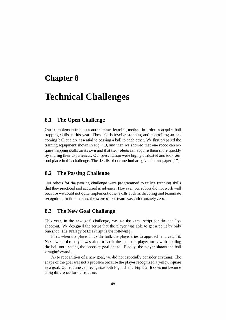
Chapter 8

Technical Challenges

8.1 The Open Challenge

Our team demonstrated an autonomous learning method in order to acquire balltrapping skills in this year. These skills involve stopping and controlling an on-coming ball and are essential to passing a ball to each other. We first prepared thetraining equipment shown in Fig. 4.3, and then we showed that one robot can ac-quire trapping skills on its own and that two robots can acquire them more quicklyby sharing their experiences. Our presentation were highly evaluated and took sec-ond place in this challenge. The details of our method are given in our paper [17].

8.2 The Passing Challenge

Our robots for the passing challenge were programmed to utilize trapping skillsthat they practiced and acquired in advance. However, our robots did not work wellbecause we could not quite implement other skills such as dribbling and teammaterecognition in time, and so the score of our team was unfortunately zero.

8.3 The New Goal Challenge

This year, in the new goal challenge, we use the same script for the penalty-shootout. We designed the script that the player was able to get a point by onlyone shot. The strategy of this script is the following.

First, when the player finds the ball, the player tries to approach and catch it.Next, when the player was able to catch the ball, the player turns with holdingthe ball until seeing the opposite goal ahead. Finally, the player shoots the ballstraightforward.

As to recognition of a new goal, we did not especially consider anything. Theshape of the goal was not a problem because the player recognized a yellow squareas a goal. Our routine can recognize both Fig. 8.1 and Fig. 8.2. It does not becomea big difference for our routine.

48

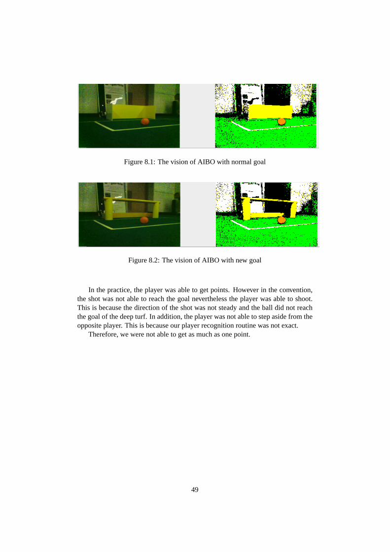
Figure 8.1: The vision of AIBO with normal goal

Figure 8.2: The vision of AIBO with new goal

In the practice, the player was able to get points. However in the convention,the shot was not able to reach the goal nevertheless the player was able to shoot.This is because the direction of the shot was not steady and the ball did not reachthe goal of the deep turf. In addition, the player was not able to step aside from theopposite player. This is because our player recognition routine was not exact.

Therefore, we were not able to get as much as one point.

49

Chapter 9

Conclusion

The team Jolly Pochie entered the finals in the RoboCup Japan Four-legged League2006. In the RoboCup Four-legged League 2006, our team won one game and lostone game in the first round robin pool.

Our mainly improvements of this year are three things. The First is more ac-curate object recognition of our vision system by improving our object recognitionalgorithms and our learning tool generating color tables. The second is more ro-bust estimation of ball’s location by utilizing a new localization technique. Thethird is work saving for developing successful ball trapping skills by utilizing anautonomous learning technique for the skills.

We will continue the development of our object recognition routine and thecombination of our soccer simulator and on machine learning techniques.

50

Bibliography

[1] Sonia Chernova and Manuela Veloso. Learning and using models of kickingmotions for legged robots. InProceedings of International Conference onRobotics and Automation, 2004.

[2] Aymeric de Cabrol, Patrick Bonnin, Thomas Costis, Vincent Hugel, PierreBlazevic, and Kamel Bouchefra. A New Video Rate Region Color Segmen-tation and Classification for Sony Legged RoboCup Application. InRoboCup2005, volume 4020 ofLNAI, pages 436–443. Springer-Verlag, 2005.

[3] F. Dellaert, D. Fox, W. Burgard, and S. Thrun. Monte Carlo Localization ForMobile Robots. InProc. of the IEEE International Conference on Robotics& Automation, 1998.

[4] M. Dietl, J.-S. Gutmann, and B. Nebel. Cooperative sensing in dynamic en-vironments. InProc. of the IEEE/RSJ International Conference on IntelligentRobots and Systems (IROS’01), 2001.

[5] A. Ferrein, G. Lakemeyer, and L. Hermanns. Comparing Sensor Fusion Tech-niques for Ball Position Estimation. InProc. of the RoboCup 2005 Sympo-sium, 2005. to appear.

[6] Peggy Fidelman and Peter Stone. Learning ball acquisition on a physicalrobot. In2004 International Symposium on Robotics and Automation (ISRA),2004.

[7] D. Fox, W. Burgard, F. Dellaert, and S. Thrun. Monte Carlo Localization:Efficient Position Estimation for Mobile Robots. InProc. of the NationalConference on Artificial Intelligence, 1999.

[8] Gregory S. Hornby, Seichi Takamura, Takashi Yamamoto, and Masahiro Fu-jita. Autonomous evolution of dynamic gaits with two quadruped robots.IEEE Transactions on Robotics, 21(3):402–410, 2005.

[9] William H. Hsu, Scott J. Harmon, Edwin Rodriguez, and Christopher Zhong.Empirical comparison of incremental reuse strtegies in genetic programmingfor keep-away soccer. InLate Breaking Papers at the 2004 Genetic and Evo-lutionary Computation Conference, 2004.

51

[10] C. Hue, J.-P. Le Cadre, and P. Perez. Tracking multiple objects with particlefiltering. Technical Report 1361, IRISA, 2000.

[11] J. Inoue, H. Kobayashi, A. Ishino, and A. Shinohara. Jolly Pochie 2005 in theFour Legged Robot League, 2005.

[12] JollyPochie —team for RoboCup soccer 4-legged robot league—.<http://www.i.kyushu-u.ac.jp/JollyPochie/>.

[13] R. Kalman. A New Approach to Linear Filtering and Prediction Problems.Journal of Basic Engineering, pages 35–45, 1960.

[14] A. Karol and M.-A. Williams. Distributed Sensor Fusion for Object Tracking.In Proc. of the RoboCup 2005 Symposium, 2005. to appear.

[15] Min Sub Kim and William Uther. Automatic gait optimisation for quadrupedrobots. InProceedings of 2003 Australasian Conference on Robotics andAutomation, pages 1–9, 2003.

[16] Hayato Kobayashi, Tsugutoyo Osaki, Akira Ishino, Jun Inoue, Naru-michi Sakai, Satoshi Abe, Shuhei Yanagimachi, Tetsuro Okuyama, AkihiroKamiya, Kazuyuki Narisawa, and Ayumi Shinohara. Jolly Pochie TechnicalReport RoboCup2005. Technical report, Jolly Pochie, 2005.

[17] Hayato Kobayashi, Tsugutoyo Osaki, Eric Williams, Akira Ishino, and AyumiShinohara. Autonomous learning of ball trapping in the four-legged robotleague. InProc. RoboCup International Symposium 2006, LNCS. Springer-Verlag, 2007. to appear.

[18] Nate Kohl and Peter Stone. Machine learning for fast quadrupedal locomo-tion. In The Nineteenth National Conference on Artificial Intelligence, pages611–616, 2004.

[19] R. Matthew Kretchmar. Parallel reinforcement learning. InThe 6th WorldConference on Systemics, Cybernetics, and Informatics., 2002.

[20] C. Kwok and D. Fox. Map-based Multiple Model Tracking of a MovingObject. InProc. of the RoboCup 2004 Symposium, 2004.

[21] T. Rofer, T. Laue, and D. Thomas. Particle-Filter-Based Self-Localization Us-ing Landmarks and Directed Lines. InRoboCup 2005: Robot Soccer WorldCup IX, Lecture Notes in Artificial Intelligence, Springer, 2005. to appear.

[22] D. Schulz, W. Burgard, D. Fox, and A.B. Cremers. Tracking Multiple Mov-ing Objects with a Mobile Robot. InProc. of the IEEE Computer SocietyConference on Robotics and Automation(ICRA), 2001.

52

[23] Christopher Stanton and Mary-Anne Williams. A Novel and Practical Ap-proach Towards Color Constancy for Mobile Robots Using OverlappingColor Space Signatures. InRoboCup 2005, volume 4020 ofLNAI, pages444–451. Springer-Verlag, 2005.

[24] Peter Stone, Richard S. Sutton, and Gregory Kuhlmann. Reinforcement learn-ing for robocup soccer keepaway.Adaptive Behavior, 13(3):165–188, 2005.

[25] Peter Stone and Manuela M. Veloso. Layered learning. InProceedings of11th European Conference on Machine Learning, volume 1810, pages 369–381. Springer, Berlin, 2000.

[26] A. Stroupe, M.-C. Martin, and T. Balch. Distributed Sensor Fusion for ObjectPosition Estimation by Multi-Robot Systems. InProc. of the IEEE Interna-tional Conference on Robotics and Automation. IEEE, 2001.

[27] Richard S. Sutton and Andrew G. Barto.Reinforcement Learning: An Intro-duction. MIT Press, 1998.

[28] Joel D. Weingarten, Gabriel A. D. Lopes, Martin Buehler, Richard E. Groff,and Daniel E. Koditschek. Automated gait adaptation for legged robots. InIEEE International Conference on Robotics and Automation, 2004.

[29] Juan Cristóbal Zagal and Javier Ruiz del Solar. Learning to kick the ball usingback to reality. InRoboCup 2004: Robot Soccer World Cup VIII, volume3276 ofLNAI, pages 335–347. Springer-Verlag, 2005.

53