Embed Size (px)
Citation preview

CESKE VYSOKE UCENI TECHNICKE V PRAZEFakulta stavebnı
Doktorsky studijnı program: STAVEBNI INZENYRSTVIStudijnı obor: Konstrukce a dopravnı stavby
Ing. Vıt Smilauer
ELASTICKE VLASTNOSTI HYDRATUJICI CEMENTOVE PASTYURCENE Z MODELU HYDRATACE
ELASTIC PROPERTIES OF HYDRATING CEMENT PASTE DETERMINED FROMHYDRATION MODELS
DISERTACNI PRACE K ZISKANI AKADEMICKEHO TITULU Ph.D.
Skolitel: Prof. Ing. Zdenek Bittnar, DrSc.
Praha, prosinec, 2005


Table of contents iii
TABLE OF CONTENTS
List of Figures vi
List of Tables ix
Notation xvi
Chapter 1: Introduction and state of the art 11.1 Microstructure observation . . . . . . . . . . . . . . . . . . . . . . . . . . . . 2
1.2 Cement hydration models . . . . . . . . . . . . . . . . . . . . . . . . . . . . . 4
1.3 Intrinsic properties . . . . . . . . . . . . . . . . . . . . . . . . . . . . . . . . 7
1.4 Homogenization theory . . . . . . . . . . . . . . . . . . . . . . . . . . . . . . 8
1.5 Elastic homogenization of cement composites . . . . . . . . . . . . . . . . . . 10
1.6 Percolation theory . . . . . . . . . . . . . . . . . . . . . . . . . . . . . . . . . 12
1.7 Organization of thesis . . . . . . . . . . . . . . . . . . . . . . . . . . . . . . . 13
Chapter 2: Hydration of cement 152.1 Chemical properties . . . . . . . . . . . . . . . . . . . . . . . . . . . . . . . . 15
2.2 Definitions . . . . . . . . . . . . . . . . . . . . . . . . . . . . . . . . . . . . . 16
2.3 Portland cement prior to hydration . . . . . . . . . . . . . . . . . . . . . . . . 17
2.4 Hydration of constituents of Portland cement . . . . . . . . . . . . . . . . . . 18
2.4.1 Hydration of C3S . . . . . . . . . . . . . . . . . . . . . . . . . . . . 18
2.4.2 Hydration of C2S . . . . . . . . . . . . . . . . . . . . . . . . . . . . 20
2.4.3 Reactions of C3A . . . . . . . . . . . . . . . . . . . . . . . . . . . . 21
2.4.4 Reactions of C4AF . . . . . . . . . . . . . . . . . . . . . . . . . . . 22
2.5 Characterization of hydration products . . . . . . . . . . . . . . . . . . . . . . 23
2.5.1 Calcium hydroxide . . . . . . . . . . . . . . . . . . . . . . . . . . . . 23
2.5.2 Calcium silicate hydrates . . . . . . . . . . . . . . . . . . . . . . . . . 24
2.6 Degree of hydration concept related to mechanical properties . . . . . . . . . . 26
Chapter 3: Modeling of cement hydration 293.1 Affinity model . . . . . . . . . . . . . . . . . . . . . . . . . . . . . . . . . . . 29
3.2 Other models based on KJMA equations . . . . . . . . . . . . . . . . . . . . . 32

Table of contents iv
3.2.1 HYMOSTRUC model . . . . . . . . . . . . . . . . . . . . . . . . . . 32
3.2.2 Pignat and Navi’s model . . . . . . . . . . . . . . . . . . . . . . . . . 34
3.3 Powers and Brownyard’s model . . . . . . . . . . . . . . . . . . . . . . . . . 34
3.4 CEMHYD3D model . . . . . . . . . . . . . . . . . . . . . . . . . . . . . . . 35
3.4.1 Implemented reactions . . . . . . . . . . . . . . . . . . . . . . . . . . 40
3.4.2 Reconstruction of initial microstructure . . . . . . . . . . . . . . . . . 41
3.4.3 Mapping hydration cycles to time . . . . . . . . . . . . . . . . . . . . 43
3.4.4 Effect of initial microstructure size . . . . . . . . . . . . . . . . . . . . 44
3.4.5 Effect of microstructure size on hydration and percolation . . . . . . . 45
3.4.6 Microscale C-S-H model based on a transition thickness . . . . . . . . 47
3.4.7 Microscale C-S-H model based on confinement . . . . . . . . . . . . . 49
Chapter 4: Homogenization of cement-based materials 524.1 Representative volume element of cement paste . . . . . . . . . . . . . . . . . 54
4.2 Percolation of solids . . . . . . . . . . . . . . . . . . . . . . . . . . . . . . . 55
4.3 Intrinsic properties of constituents . . . . . . . . . . . . . . . . . . . . . . . . 57
4.3.1 C-S-H mechanical properties . . . . . . . . . . . . . . . . . . . . . . . 58
4.3.2 Cement paste level . . . . . . . . . . . . . . . . . . . . . . . . . . . . 59
Chapter 5: Analytical homogenization methods 625.1 Rule of mixtures . . . . . . . . . . . . . . . . . . . . . . . . . . . . . . . . . 65
5.2 Hashin-Shtrikman and Walpole bounds . . . . . . . . . . . . . . . . . . . . . 65
5.3 Mori-Tanaka method . . . . . . . . . . . . . . . . . . . . . . . . . . . . . . . 66
5.4 Self-consistent scheme . . . . . . . . . . . . . . . . . . . . . . . . . . . . . . 67
5.5 N-layered spheres . . . . . . . . . . . . . . . . . . . . . . . . . . . . . . . . . 69
5.6 Other elastic homogenization models . . . . . . . . . . . . . . . . . . . . . . . 70
Chapter 6: Numerical homogenization methods 736.1 General principles and material isotropy . . . . . . . . . . . . . . . . . . . . . 73
6.2 Eigenstrain method . . . . . . . . . . . . . . . . . . . . . . . . . . . . . . . . 74
6.3 Smaller volume then the representative volume element . . . . . . . . . . . . . 76
6.4 FEM eigenstrain procedure for periodic boundary conditions . . . . . . . . . . 77
6.4.1 Numerical verification . . . . . . . . . . . . . . . . . . . . . . . . . . 79
6.4.2 Implementing phase disconnectedness . . . . . . . . . . . . . . . . . . 82
6.5 Static and kinematic uniform boundary conditions . . . . . . . . . . . . . . . . 83
6.6 FFT-based homogenization . . . . . . . . . . . . . . . . . . . . . . . . . . . . 84

Table of contents v
Chapter 7: Validation 877.1 Cement paste level . . . . . . . . . . . . . . . . . . . . . . . . . . . . . . . . 87
7.1.1 Homogenization of RVE with random distribution of solids . . . . . . 87
7.1.2 Paste of Kamali et al., w/c = 0.5 . . . . . . . . . . . . . . . . . . . . . 90
7.1.3 Paste of Kamali et al., w/c = 0.25 . . . . . . . . . . . . . . . . . . . . 94
7.1.4 Paste of Boumiz, w/c = 0.40 . . . . . . . . . . . . . . . . . . . . . . . 97
7.1.5 Paste of Boumiz, w/c = 0.35 . . . . . . . . . . . . . . . . . . . . . . . 98
7.1.6 BAM cement paste, w/c = 0.3 . . . . . . . . . . . . . . . . . . . . . . 99
7.1.7 Pignat’s paste, w/c = 0.45 . . . . . . . . . . . . . . . . . . . . . . . . 101
7.1.8 Performance of two hydration models, w/c = 0.5 . . . . . . . . . . . . 103
7.1.9 Leaching of cement pastes . . . . . . . . . . . . . . . . . . . . . . . . 104
7.2 Initial stress concentration . . . . . . . . . . . . . . . . . . . . . . . . . . . . 106
7.3 Mortar level incorporating ITZ . . . . . . . . . . . . . . . . . . . . . . . . . . 108
7.3.1 Mortar by Yang, w/b = 0.3 . . . . . . . . . . . . . . . . . . . . . . . . 109
7.3.2 Mortar B60 of Boumiz, w/c = 0.387 . . . . . . . . . . . . . . . . . . . 111
7.3.3 Mortar B35 of Boumiz, w/c = 0.524 . . . . . . . . . . . . . . . . . . . 112
7.4 Concrete level . . . . . . . . . . . . . . . . . . . . . . . . . . . . . . . . . . . 114
Chapter 8: Conclusion and future work 117
Bibliography 120
Appendix A: Herve-Zaoui scheme 133

List of figures vi
LIST OF FIGURES
1.1 The correlation between compressive strength and modulus of elasticity . . . . 3
2.1 Hydration of C3S from the first contact with water to its late period . . . . . . . 19
2.2 Locher’s mineralogical model of early C3A hydration . . . . . . . . . . . . . . 21
2.3 Strength vs. capillary porosity for normally cured cement pastes . . . . . . . . 28
3.1 Evolution of the microstructure in HYMOSTRUC model . . . . . . . . . . . . 33
3.2 A flowchart of CEMHYD3D model and the homogenization process . . . . . . 37
3.3 Microstructure 50 × 50 × 50 µm, w/c = 0.25 . . . . . . . . . . . . . . . . . . 38
3.4 Results of three models on pure C3S hydration, w/c = 0.42 . . . . . . . . . . 40
3.5 PSD for German cements, all cements are type I . . . . . . . . . . . . . . . . . 42
3.6 PSD for German cements from the NIST database . . . . . . . . . . . . . . . . 42
3.7 Relative error in the degree of hydration in different RVE . . . . . . . . . . . . 46
3.8 Unhydrated part of particles with specified diameter . . . . . . . . . . . . . . . 46
3.9 Percolation of two microstructures with different RVE sizes . . . . . . . . . . . 47
3.10 Hydration evolution in five realizations for two RVE sizes, w/c = 0.5 . . . . . 48
3.11 Hydration evolution in five realizations for two RVE sizes, w/c = 0.25 . . . . 48
3.12 Predicted relative volumetric ratio of C-S-HLD in cement pastes . . . . . . . . 49
3.13 C-S-HHD evolution in three w/c’s in dependence on surrounding solid volume . 51
3.14 C-S-HHD evolution depending on the neighborhood selection . . . . . . . . . . 51
4.1 Images of C-S-H, cement paste and mortar level . . . . . . . . . . . . . . . . . 53
4.2 Released heat, simulation and typical percolation curve . . . . . . . . . . . . . 56
4.3 C-S-H nanoindentation data, w/c = 0.5 . . . . . . . . . . . . . . . . . . . . . 58
5.1 Material with particulate structure . . . . . . . . . . . . . . . . . . . . . . . . 67
5.2 Material with skeletal structure . . . . . . . . . . . . . . . . . . . . . . . . . . 67
5.3 Performance of self consistent scheme with and without solid percolation . . . 68
5.4 The geometrical representation of the 3-layered Herve-Zaoui scheme . . . . . . 70
5.5 Homogenization of an aggregate with a soft phase . . . . . . . . . . . . . . . . 72
5.6 Homogenization of an aggregate with hydrating cement paste . . . . . . . . . . 72
6.1 FEM implementation of voxelized microstructure . . . . . . . . . . . . . . . . 78

List of figures vii
6.2 Displacements on checkerboard structure using linear hexahedral element . . . 80
6.3 Displacements on checkerboard structure using quadratic hexahedral element . 81
6.4 FEM evolution of E, ν at w/c = 0.5, unpercolated input images . . . . . . . . . 81
6.5 FEM evolution of E, ν at w/c = 0.25, unpercolated input images . . . . . . . . 81
6.6 Possible configuration of split nodes in adjacent voxels . . . . . . . . . . . . . 83
6.7 Example of percolation in 2D microstructure at early ages . . . . . . . . . . . 83
6.8 Normalized norm of residuum in the CGM . . . . . . . . . . . . . . . . . . . . 84
6.9 Homogenized isotropic Young’s modulus and error during FFT . . . . . . . . . 86
7.1 Middle slice of analyzed two-phase digital images . . . . . . . . . . . . . . . . 88
7.2 Effect of microstructure size on percolation . . . . . . . . . . . . . . . . . . . 91
7.3 Young’s modulus, analytical homogenization, un/percolated microstructure . . 91
7.4 Hashin-Shtrikman-Walpole upper bounds and Voigt bound . . . . . . . . . . . 92
7.5 Effect of percolation on E modulus, 25 × 25 × 25 µm, FEM - periodic . . . . 92
7.6 Effect of RVE size on E modulus, FEM - periodic, split nodes, FFT . . . . . . 92
7.7 Effect of boundary conditions, α = 0.3 (a) and 0.9 (b), FEM, split nodes . . . . 93
7.8 Difference among uniform, split node mesh and FFT . . . . . . . . . . . . . . 94
7.9 Analytical results from the C-S-H level . . . . . . . . . . . . . . . . . . . . . 95
7.10 Analytically predicted Young’s modulus of cement paste, compared to FFT . . 95
7.11 Solid percolation of microstructures of different sizes . . . . . . . . . . . . . . 95
7.12 Effect of RVE size on E modulus, FEM - periodic, split nodes, FFT . . . . . . 95
7.13 Effect of boundary conditions, FEM, split nodes . . . . . . . . . . . . . . . . . 96
7.14 Difference among uniform, split node mesh and FFT . . . . . . . . . . . . . . 96
7.15 Volumetric content of chemical phases during hydration . . . . . . . . . . . . . 97
7.16 Homogenization of rescaled images from 25 × 25 × 25 µm . . . . . . . . . . 97
7.17 Results from FFT-based homogenization, percolated 75 × 75 × 75 µm . . . . . 98
7.18 Analytically predicted Young’s modulus, w/c = 0.35 . . . . . . . . . . . . . . 98
7.19 Analytically predicted Poisson’s ratio, w/c = 0.35 . . . . . . . . . . . . . . . 98
7.20 Effect of resolution, dissolution neighborhood and RVE size . . . . . . . . . . 99
7.21 Results from simulations and experiments . . . . . . . . . . . . . . . . . . . . 100
7.22 Predicted and measured elastic properties, FEM, FFT . . . . . . . . . . . . . . 100
7.23 PSD fit for coarse and fine cement, according to R-R distribution . . . . . . . . 101
7.24 Typical microstructure slice 100× 100 from the C3S cement paste . . . . . . . 102
7.25 Young’s modulus and Poisson’s ratio for the coarse C3S cement paste . . . . . 102
7.26 Coarse and fine microstructure of C3S paste . . . . . . . . . . . . . . . . . . . 104
7.27 Volumetric fractions, Young’s modulus and bulk modulus . . . . . . . . . . . . 105

List of figures viii
7.28 Relationship between compressive strength and coarse capillary porosity . . . . 108
7.29 The morphology of ITZ of the concrete . . . . . . . . . . . . . . . . . . . . . 109
7.30 Effect of ITZ thickness and Young’s modulus reduction . . . . . . . . . . . . . 111
7.31 Development of E modulus in plain cement paste, FFT homogenization . . . . 112
7.32 Effect of ITZ on the homogenized elastic properties of mortar . . . . . . . . . 112
7.33 Released heat during early-ages . . . . . . . . . . . . . . . . . . . . . . . . . 113
7.34 Effect of ITZ properties on the homogenized elastic properties of mortar . . . . 113
7.35 Young’s modulus of cement paste, mortar and concrete, w/c = 0.5 . . . . . . . 115
7.36 Young’s modulus of cement paste, mortar and concrete, w/c = 0.27 . . . . . . 116
8.1 Young’s moduli of analyzed cement pastes . . . . . . . . . . . . . . . . . . . . 118
8.2 Young’s moduli from the FFT homogenization with the fit . . . . . . . . . . . 119

ix
LIST OF TABLES
2.1 Compound properties used in cement chemistry . . . . . . . . . . . . . . . . . 15
2.2 Typical composition of silicate clinker or cement . . . . . . . . . . . . . . . . 17
2.3 Stages in the hydration process of C3S . . . . . . . . . . . . . . . . . . . . . . 19
2.4 The effect of gypsum on C3A hydration products . . . . . . . . . . . . . . . . 21
3.1 Apparent activation energy for concrete made from the cement CEM I 42.5 . . 30
3.2 Parameters for affinity model of cement hydration . . . . . . . . . . . . . . . . 31
3.3 Particle diameter statistics in a C3S cement powder . . . . . . . . . . . . . . . 45
3.4 Effect of RVE size in a C3S cement powder with two finenesses and two w/c’s 45
3.5 Portland cement input parameters used in the C-S-H model verification . . . . 50
4.1 Determination of degree of hydration at the solid percolation threshold . . . . . 57
4.2 Downscaling of C-S-HLD and C-S-HHD to the building units . . . . . . . . . . 59
4.3 Intrinsic elastic moduli of chemical phases . . . . . . . . . . . . . . . . . . . . 60
5.1 Homogenization with different phase order on a three phase system . . . . . . 69
6.1 FEM results from checkerboard configuration, linear approximations . . . . . . 79
6.2 FEM results from checkerboard configuration, quadratic approximations . . . . 80
7.1 Effective properties of a two-phase material . . . . . . . . . . . . . . . . . . . 89
7.2 Effective properties of a three-phase material with a grain radius of 10 µm . . . 89
7.3 Effective properties of a three-phase material with a grain radius of 20 µm . . . 90
7.4 Cement parameters for Kamali’s microstructure reconstruction . . . . . . . . . 90
7.5 Approximate computational requirements between FEM and FFT . . . . . . . 94
7.6 Cement parameters for Boumiz’s microstructure reconstruction . . . . . . . . . 97
7.7 Input parameters for German cement microstructure reconstruction . . . . . . . 100
7.8 Results from sound and leached cement pastes . . . . . . . . . . . . . . . . . . 106
7.9 Results of MHH analysis for w/c = 0.5 and 0.25 . . . . . . . . . . . . . . . . 107
7.10 Effect of ITZ properties in a cement mortar . . . . . . . . . . . . . . . . . . . 110
7.11 Input parameters for Boumiz’s cement in B60 mortar . . . . . . . . . . . . . . 111
7.12 Mortar composition in 1 m3, w/c = 0.387 . . . . . . . . . . . . . . . . . . . . 112
7.13 Input parameters for Boumiz’s cement in B35 mortar . . . . . . . . . . . . . . 113

x
7.14 Mortar composition in 1 m3, w/c = 0.524 . . . . . . . . . . . . . . . . . . . . 113
7.15 Cement specification and concrete composition in 1 m3, w/c = 0.5 and 0.27 . . 114

Acknowledgments xi
ACKNOWLEDGMENTS
Before all other acknowledgements, I would like to express my gratitude to my thesis advi-
sor, Prof. Ing. Zdenek Bittnar, DrSc., who inspired me with novel ideas from research and needs
from engineering society. He has managed several workshops at the Czech Technical Univerity
in Prague and invited me to interesting international conferences where fruitful discussions with
other specialists were possible and motivated me to several improvements.
Several personalities from the university influenced the content of this thesis. Special thanks
belong to Prof. Ing. Jirı Sejnoha, DrSc. for his perfect lectures about material engineering, Doc.
Ing. Petr Kabele, Ph.D. for many fruitful discussions, Prof. Ing. Milan Jirasek, Ph.D. for swift
questions and deep insight, Doc. RNDr. F. Skvara, DrSc. for answering the questions from ce-
ment chemistry, Ing. Jan Zeman, Ph.D. for much inspiration and many suggestions dealing with
homogenization, Mgr. Ing. Martin Wierer, Ph.D. for the implementation of several algorithms,
Ing. Jaroslav Kruis, Ph.D. for the help with FEM and other program implementations, Doc.
Dr. Ing. Dan Rypl for the implementation and explanation of mesh generator, Doc. Ing Borek
Patzak, Ph.D. and Ing. Ladislav Svoboda for the help with programming, RNDr. L. Kopecky
for SEM photos and image analysis from electron microscope, Ing. Jirı Nemecek, Ph.D. for
nanoindentation and specimen preparation and Ing. K. Forstova for AFM and image analysis,
among others.
D.P. Bentz and E.J. Garboczi are gratefully acknowledged for the open-source code of ce-
ment hydration program CEMHYD3D that gathered pieces of knowledge from cement physics
and chemistry and used the new insight in hydration modeling. As the workshop organizers in
Gaithersburg, MA, they allowed me to attend this interesting annual workshop in 2003 where I
had the opportunity to meet several researchers and personalities.
I would like to thank Prof. Karen Scrivener and her staff, particularly S. Bishnoi, from
EPFL who organized my stay at Lausanne in 2005 and have managed the NANOCEM con-
sortium where the possibility of information exchange among similarly oriented researchers
is appreciated. I esteem highly the initiation of Prof. K. van Breugel from TU Delft in the
modeling of cement hydration.
I gratefully acknowledge the financial support from the Ministry of Education, Youth and
Sports in the grant MSM 6840770003 – Algorithms for computer simulation and application
in engineering. At last, I appreciate encouragement, suggestions and patience of my relatives,
particularly my parents, my sister Anna, brother Vaclav and my wife Adela.

Abstract xii
Czech Technical University in Prague
Faculty of Civil Engineering
Abstract
Elastic properties of hydrating cement paste determined from hydration models
by Vıt Smilauer
This Ph.D. thesis attempts to apply elastic homogenization methods for the prediction of elastic
properties of the microstructures of cement-based materials. The latter may be analyzed on four
independent scales, based on a characteristic length criterion; C-S-H level, cement paste level,
mortar level and concrete level. The thesis focuses on the cement paste level, where the majority
of changes occurs during the hydration. The homogenization procedure is complicated by the
fact that the liquid suspension of the cement mixture is transformed to a solid, load-bearing
structure, being in the category of porous materials.
The reconstruction of cement paste microstructures is based purely on the 3D discrete hy-
dration program called CEMHYD3D, released by NIST organization. At this level, it is possible
to capture the particle size distribution, effect of cement chemical composition, curing temper-
ature or curing water regime. Other vector models based on Avrami equation are proposed and
compared on a few examples with the NIST model. The effect of various initial microstructure
sizes on statistical descriptors is examined throughout. Moreover, the variations of degree of
hydration among differently sized microstructures lead to the definition of reasonable sizes of
representative volume element, too. A new model of C-S-HLD and C-S-HHD evolution at the
microscale is presented and validated with the results from porosimetry.
Recent advances in nanoindentation provided the intrinsic elastic properties of major con-
stituents of unhydrated and hydrated cement paste. The homogenization in this thesis is based
on three approaches. The first one assumes certain special morphological configurations result-
ing in analytical methods as the Mori-Tanaka or the self-consistent scheme. Perfect results were
obtained at the C-S-H level for upscaling from C-S-H building units. The second approach is
based on the FEM where static, kinematic or periodic boundary conditions are applied. The
periodic conditions were found as the best approximation of reality, even in small representa-
tive volumes. Special mesh generator accounting for the percolation in early hydration ages is
designed, enabling homogenization from the final set point of the cement paste.
The third homogenization method is based on FFT transformation of periodic strain and
stress fields on a periodic microstructure. Compared to FEM, field approximations are not
limited by any shape functions, also no assemblage of stiffness matrix has to be carried out.

Abstract xiii
The results are mutually comparable with significant savings in both computational time and
memory.
Several examples from the literature are validated showing the potential of homogenization
methods. Microstructures from C3S paste as obtained from two different hydration models are
compared and the differences are discussed. Beyond the homogenization of standard cement
pastes, the leached cement pastes are analyzed. The mortar level is treated analytically, includ-
ing the interphase transition zone around the fine aggregates. Similar approach at the concrete
level leads to good estimations of elastic properties during the whole hydration period of con-
crete.

Abstrakt xiv
Ceske vysoke ucenı technicke v Praze
Fakulta stavebnı
Abstrakt
Elasticke vlastnosti hydratujıcı cementove pasty urcene z modelu hydratace
Vıt Smilauer
Tematem teto prace je pouzitı elastickych metod homogenizace pro predpoved’ elastickych
vlastnostı mikrostruktur materialu zalozenych na cementu. Tyto materialy mohou byt ana-
lyzovany ve ctyrech nezavislych urovnıch na zaklade kriteria charakteristicke delky: C-S-H
uroven, uroven cementove pasty, uroven malty a betonu. Prace se soustred’uje na uroven cemen-
tove pasty, kde se odehrava vetsina zmen behem hydratace. Homogenizace je komplikovana
faktem, ze kapalna suspenze cementove smesi se menı do pevne faze, ktera je schopna prenaset
zatızenı, a ktera spada do skupiny poreznıch materialu.
Vytvorenı mikrostruktury cementove pasty je ciste zalozeno na prostorovem diskretnım hy-
dratecnım programu CEMHYD3D, poskytnutym organizacı NIST. Na teto urovni je mozno
zachytit krivku zrnitosti, ucinek chemickeho slozenı cementu, ucinek teploty nebo vodnıho
rezimu. Jsou formulovany dalsı spojite hydratacnı modely zalozene na Avramiho rovnici a
porovnany na nekolika prikladech s NIST modelem. Ucinek ruznych pocatecnıch velikostı
mikrostruktur na statistickych ukazatelıch je podrobne prozkouman. Navıc variace stupne
hydratace mezi ruznymi velikostmi mikrostruktur vede rovnez k definici vhodnych velikostı
reprezentativnıch objemu pro simulaci. Je uveden novy model pro vyvoj C-S-HLD a C-S-HHD
na mikromerıtku a porovnan s vysledky z porozimetrie.
Nedavne pokroky v nanoindentaci poskytly udaje o charakteristickych elastickych vlastnos-
tech hlavnıch slozek nehydratovane a zhydratovane cementove pasty. Homogenizace je v teto
praci zalozena na trech prıstupech. Prvnı predpoklada urcitou specialnı konfiguraci morfologie,
ktera ustı do analytickych metod jako Mori-Tanaka nebo “samokonzistentnı” (self-constistent).
Vyborne vysledky byly dosazeny na urovni C-S-H pri skalovanı z C-S-H stavebnıch jednotek.
Druhy prıstup je zalozen na metode konecnych prvku, kde jsou uplatneny staticke, kinematicke
ci periodicke okrajove podmınky. Periodicke podmınky se nejlepe blızı skutecnemu chovanı a
to dokonce v malych reprezentativnıch objemech. Je vytvoren specialnı generator sıtı zahrnujıcı
perkolaci v ranych stadiıch hydratace, ktery umoznuje homogenizaci jiz od konce tuhnutı.
Tretı homogenizacnı metoda je zalozena na Fourierove transformaci periodickych polı de-
formacı a napetı na periodickych mikrostrukturach. V porovnanı s metodou konecnych prvku
nejsou aproximace polı omezeny interpolacnımi funkcemi posunu ani nenı potreba sestavovat

Abstrakt xv
matici tuhosti. Vysledky jsou srovnatelne s podstatne mensımi naroky na cas a pamet’.
Schopnosti homogenizacnıch metod jsou overeny na mnozstvıch prıkladu z literatury. Mik-
tostruktury C3S pasty ze dvou rozdılnych homogenizacnıch modelu jsou porovnany a rozdıly
vysvetleny. Krome homogenizace obycejnych cementovych past jsou analyzovany vyluho-
vane pasty. Uroven malty je resena analyticky se zahrnutım prechodove zony okolo zrn pısku.
Podobny prıstup na urovni betonu vede k dobrym odhadum elastickych vlastnostı behem cele
hydratace.

Notation xvi
NOTATION
Material elastic properties
E Young’s modulus
ν Poisson’s ratio
k bulk modulus
µ shear modulus
Tensor notation
u first-order tensor, e.g. a displacement tensor
σ second-order tensor, e.g. a stress tensor
C fourth-order tensor, e.g. a stiffness tensor
Matrix algebra notation
r vector, e.g. a displacement vector
K matrix, e.g. a stiffness matrix
Cement terminology
w/c water-to-cement ratio (the mass fraction of water to cement)
w/b water-to-binder ratio (in case not only cement is used as a binder)
ITZ interfacial transition zone
PSD particle size distribution
OPC ordinary Portland cement
CH calcium hydroxide or portlandite
C-S-H calcium silica hydrates
C-A-H calcium aluminate hydrates
Cement chemistry abbreviation
Al2O3 = A Fe2O3 = F MgO = M SiO2 = S
CaO = C H2O = H Na2O = N SO3 = S
CO2 = C K2O = K P2O5 = P TiO2 = T

Introduction and state of the art 1
Chapter 1
INTRODUCTION AND STATE OF THE ART
Concrete is undoubtedly one of the most demanded, favorite and universal engineering ma-
terial today. The term “concrete” symbolizes a wide range of composite materials starting from
asphalt matrix and going to fly-ash mixtures. Concrete belongs to the category of porous mate-
rials where the capillary porosity may attain values up to 30 % in the case of normal hardened
Portland cement paste. The next discussion will deal dominantly with the Portland cements and
derived composites such as mortar or concrete. Since concrete is a complex material, a wide
range of science disciplines is needed for comprehensive understanding; cement and physical
chemistry, image processing techniques, modeling, computer science or mechanical engineer-
ing.
The historical origin of cement is unclear but documented that Assyrians, Babylonians,
Chinese and Egyptians used clay or lime materials for constructions several thousands years
BC. Around 200 BC, the Romans started to use pozzolanic volcanic ash which significantly
improved material durability and for the reason that it hardened under water. Little progress oc-
curred during the middle ages until the mid of 18th century, when John Smeaton from England
discovered excellent properties of cement made from clay-rich limestone. He rebuilt Eddy-
stone Lighthouse in Cornwall, England. Vicat prepared artificial hydraulic lime in 1812–13
from synthetic mixture of limestone and clay. Joseph Aspdin of England invented in 1824 Port-
land cement, named after the building stones quarried at Portland, England. Joseph Monier
reinforced flower pots in 1867 with iron bars. In 1887, Henri Le Chatelier established oxide
ratios for proper dosing of lime to produce Portland cement. He is considered as the founder
of cement chemistry. The gypsum was introduced in 1890 in the USA to act as a retardant
of concrete setting. In 1930, the entrained air is firstly used to decrease freeze-thaw damage.
In 1940’s Powers and Brownyard formulated macroscopic hydration model that was able to
quantify hydration products and separate non-evaporable, gel, and capillary water [92]. Neville
summarized the comprehensive knowledge about concrete in a famous book in 1963, reprinted
and extended several times [79]. Lea from 1935 and Taylor from 1963 summarized knowledge
of cement chemistry resulting in the well-known books, several times reprinted [66, 110]. The
silica fume, as a pozzolanic additive, and superplasticizers were introduced in 1980’s.
Concrete is a living material due to the interaction with the water, even after many years

Microstructure observation 2
after the placing. The process of hardening is known as hydration where calcium silicates and
aluminates form hydration products, called hardened cement paste. The chemical composition
of the latter differs strongly on the source composition and usually in Portland cements con-
sists of calcium silica hydrates (C-S-H), calcium hydroxide, ettringite, and pores. The hardened
cement paste determines to a great extent various resulting properties of concrete such as me-
chanical response or permeability. The aggregates in concrete are rather intact by surrounding
reactions with an exception of detrimental alkali-silica reactions.
Today’s limits of mechanical properties of concrete lie somewhere in reactive powder con-
crete (RPC) sometimes called ultra-high performance concrete (UHPC). Large aggregates are
replaced by small steel fibers that inhibit the weak contact zone and stress concentration. Sand
fraction of concrete is carefully selected in order to increase the packing of particles and under
normal circumstances the maximum sand diameter is 600 µm. As a consequence, these compact
brittle materials attain compressive strength up to 800 MPa and are very durable compared to
ordinary concrete. Tensile strength lies between 6–13 MPa, even maintained when a first crack
occurs due to distributed steel fibers. On the other hand, the elastic properties of RPC were
found for mature concrete as low as 60 GPa regardless of fiber presence [125]. The studied
material behaved very closely to the isotropic state.
Generally, elastic properties limit the concrete application in large-span structures, e.g.
bridges or large slabs. The modification of elastic properties during fabrication is a very dif-
ficult task and with very limited improvements, demonstrated by Fig. 1.1. The mechanism of
interaction between different mechanical phases in cement paste and consequently in concrete
is described by intrinsic properties that remain in narrow ranges for the variety of concretes and
curing conditions [17]. Therefore, the micromechanical analysis of various concretes seems to
be accurate enough worldwide.
1.1 Microstructure observation
Advances in observation techniques often coincide with the progress of understanding con-
crete performance and underlying principles. Some properties known from the macroscale can
be found on the lower scale in the microstructure.
Concrete porosity spans typically several orders of magnitude, ranging from nanometer gel
pores to the millimeter air voids. The porosity changes even the hydration was ceased and may
become later refined [101]. Porosity determines to a great extent almost all of the engineer-
ing properties. For the purpose of pore or microstructure reconstruction, various techniques
were used extensively. The first group that requires a dried specimen is based on intrusion,
e.g. mercury intrusion porosimetry, pyknometry, gas sorption. More-advanced, non-destructive

Microstructure observation 3
Figure 1.1: The correlation between compressive strength and modulus of elasticity for high-
strength concrete [114]
methods use probing particles or fields (small-angle scattering, NMR, image analysis).
The mercury intrusion porosimetry (MIP) has been commonly used tool for obtaining pore
size distribution. It was observed, that revealed pore structure does not correspond to the real
structure due to inappropriate assumptions. The measured results of surface area of cement
paste using porosimetry differs in the order of two magnitudes, depending on the interpretation
and used intrusion agent [113]. Using the high pressures up to 300 MPa for MIP, the microstruc-
ture is often damaged. On the other hand, the gas sorption technique is reliable up to 30 nm
pore size [113].
The non-destructive image analysis, based on stereological principles, came into favor later.
When material is of isotropic and random nature, the 2D area is equal to the 3D volume frac-
tions. The pioneering work of image analysis was laid down by Scrivener and Pratt [104].
The same technique was extended to access the geometric features of various chemical phases,
especially within easily distinguishable unhydrated cement particles, CH crystals, C-S-H and
capillary porosity [64]. Image analysis formed the basis of vector and digital hydration models
and by today is very efficient in microstructure reconstruction, extended by means of statistical
functions. The limit of image analysis using back-scattered electrons is around 500 nm for the
cement paste. Correlation between phase amount and the microstructure was found to be in a
good agreement with the Powers hydration model [53].
Small angle scattering is based either on a diffraction of neutrons (SANS) or X-rays (SAXS).
The thickness of cement paste specimen is around 0.5 mm and the resolution can be in the order
of nanometers or higher. The important contribution of the technique is the fact, that C-S-H

Cement hydration models 4
exhibit a disordered fractal structure [112]. In addition, an increase of C-S-H surface area
occurs with increasing w/c in the range from 0.35 to 0.7 at 28 days, as opposed to a nearly
constant value of H2O sorption data [101].
Nuclear magnetic resonance has been used for measuring the chain length of C-S-H. The
average length increases with the higher initial amount of silica fume or fly ash [90]. The pore
structure of the reactive powder concrete via NMR was found to have a fractal dimension [91].
The hydration products, often denoted as C-S-H gel, are responsible for the majority of
concrete properties: strength, brittleness, elasticity, permeability, aging, shrinkage. The high
surface area of hundreds of meters per gram also generates high disjoining pressures due to
hindered absorbed water and is probably the origin of creep. This concept of microprestress
was found successful in creep prediction models [3]. Experimental observation of Le Chatelier
in 1887 noted unhydrated clinker minerals and gelatinous character of hydrates. A groups of
researchers led by T.C. Powers from 1936 found the gel pore volume to be around 28 % and
formulated a colloidal C-S-H model with the particle radius of 5 nm [92]. Today, the radius
of C-S-H globule is estimated as 3.3 nm and the gel pore volume occupies 42 % in a low
density type of C-S-H [101]. Taylor presented the layered model of C-S-H that was capable of
describing a disordered structure and a pore network [110]. Brunauer thought of a sheet C-S-H
structure that changes in a rolled fiber upon a lack of water, explaining the irreversible C-S-H
shrinkage. Feldman and Sereda proposed a similar layered model of C-S-H made of irregular
sheets [33]. According to this model, the water can re-enter the interlayer space. Although the
C-S-H originate is various types of cements, physical characteristics of C-S-H are influenced to
a minor extent by chemical composition [41].
Tennis and Jennings proposed a more quantitative colloid model of two C-S-H types in year
2000 [113]. Building units have approximately 5.6 nm across in the diameter. Depending on
the stereological configuration and confinement during hydration, the low (LD) or high den-
sity (HD) type of C-S-H is formed. The more-opened fractal structure of the C-S-HLD is more
permeable, unstable and with lower elastic modulus, as verified by mechanical nanoindentation
of the C-S-H gel [24]. The model is consistent with various commonly used techniques for
accessing the surface area, can predict the water content and density in dependence on a rela-
tive humidity. The structure of C-S-H gels is not throughout completely examined and more
advanced models may show up [113].
1.2 Cement hydration models
The first coherent and quantitative model for the hydration of cement was deduced by T.C.
Powers and his co-workers from data based on water adsorption isotherms [92]. Powers has al-

Cement hydration models 5
ready distinguished capillary, gel and non-evaporable water. Powers calculated that the 1 cm3
of Portland cement under the room temperature curing produces 2.13 cm3 of hydration prod-
ucts, on average. He stated that for the complete filling of available capillary pore space with
hydration products, the w/c of 0.36 is the threshold value. Powers also calculated the poros-
ity of cement gel to be 28 %. Knowing the degree of hydration or indirectly the fraction of
non-evaporable water, the volumetric fractions of cement gel, gel water, non-evaporable water,
unhydrated cement may be quantified. Two restraints on the hydration process were formulated
• depletion of available space for hydration products,
• insufficient water supply.
The consequence of these facts results in the maximum available degree of hydration for a given
w/c. By today, these finding are valid for the Portland cements cured at a room temperature.
The Powers model was later refined by Feldman and Sereda [33]. All of the above-mentioned
models determined to a more or less sophisticated level the volumetric fractions of cement
paste components. However, the time evolution of hydration and the kinetics of ongoing pro-
cesses were formulated later based on the Avrami-Erofeev and Kolmogorov-Erofeev models
[2, 19]. Today, these models result in equation, referred to as Kolmogorov-Johnson-Mehl-
Avrami (KJMA). These models aimed at describing the evolving crystals during recrystalliza-
tion and were successfully transferred to the cement-based materials. The formulation is based
on the following assumptions
• random distribution of particles in space,
• growing volume is decreased proportionally with the fraction that has already been trans-
formed.
After mixing with water, cement undergoes dissolution and ions are immediately liberated
into the pore water. A very thin layer of C-S-H surrounds now each cement grain, defending the
progress of reaction. The mechanism of subsequent dormant period remains the topic of many
debates and probably the secondary C-S-H growth causes the cement to thicken. Basically,
the theories attempting to explain this phenomenon fall in two categories: protective coating
theories and delayed nucleation theories [93, 110].
The first subclass of coating theories is based on observation that C-S-H appear in many
morphological forms. Different C-S-H morphologies are linked with various permeabilities,
therefore controlling the hydration progress. Jong et al. [56] proposed a mechanism where the
C-S-H experience three phase transformations, in dependence on the CH content. Since the
phase transformation is accompanied by e.g. heat flow or ion consumption, experimental data
Cement hydration models 6
would verify these hypotheses. However, these changes were unnoticed by many researchers,
by means of chemical, physical or mechanical testing, e.g. [24, 30, 38, 93, 110], and this theory
seems now to be out of date.
The osmotic pressure or membrane hypothesis belongs to the subclass of protective coating
theories. Powers [92] again assumes the thin C-S-H shell around the grains, later elaborated
by Double et al. [28]. Smaller ions, such as water or calcium, may easily diffuse through the
shell but the larger silica ions remain captured. At the end of the induction period, the osmotic
pressure causes a rupture of the thin shell and secondary C-S-H formation.
Delayed nucleation theories are a common name for many theories where calcium ions
concentration in the solution stimulates the C-S-H growth. CH precipitates at the end of the
induction period from supersaturated solution and subsidies C-S-H formation. Another insight
supports a hypothesis that CH is in a metastable stage and therefore not in the equilibrium. Due
to the energy barrier of nucleation, the C-S-H nucleation is delayed. Many researchers agree
that calcium ions play the most important role in C3S hydration, e.g. [93, 110].
The hydration models, as a prerequisite for the microstructure reconstruction, fall in two
categories: vector and discrete. Historically, the conceptually simpler vector models were
found capable of microstructure and hydration kinetics predictions, e.g. C3S hydration model of
Preece et al. [93], HYMOSTRUC by van Breugel [21], C3S model of Pignat and Navi [87] or
DuCOM hydration model by Maekawa [70]. The advantage of these models was found in sim-
plicity, computational speed and vector space; tight governing physical processes and restricted
material inputs are the disadvantages.
Kondo, Taplin, Bezjak [19], Knudsen, van Breugel [21], among others, applied the KJMA
equation for the simulation of cement hydration. They noted that after some hydration time,
the reactions change from the boundary to the diffusion-controlled ones. A decrease of dif-
fusion was ascribed to the densification of hydration products due to confined space. In a
polyphase system, two extremes were formulated: independent hydration of components and
equal fractional rates concept. The reality seems to be somewhere between and without an
explicit modeling one concept remains a necessary assumption [21].
Work of De Schutter and Taerwe [103] is an example of empirical model that described
a released heat of reaction. They superimposed reactions of Portland cement with slag reac-
tions, yielding two sets of three parameters. The physical meaning of fitted parameters remains
usually unclear in empirical hydration models.
Several principles from vector models were extended and the microstructure discretized
enabling more local control over the physical processes and chemical reactions. Tzschichholz
et al. [119] formulated a heterogeneous reaction-diffusion model for the setting and hydration

Intrinsic properties 7
of cement. The physical principles of diffusion ion transport and chemical dissolution and
precipitation reactions frame the model. The initial digital microstructure is used as well with
the size typically between 1 and 100 µm. Having for example the reaction of C-S-H formation,
the inequality of equilibrium solubility product and ion concentration determines the dissolution
or precipitation of C-S-H within each volume element of the model. The dissolution reactions
possess the dissolution constants of individual phases.
One of the most remarkable model is CEMHYD3D, developed in 1990’s at NIST [8]. The
model has provided valuable data about microstructure depercolation and found an unique rela-
tionship between the capillary porosity and percolation for the various w/c’s [11]. Similarly, the
model found that alkali-rich cements cause sooner depercolation of microstructure thus proba-
bly the change of C-S-H morphology to the lath-like type [13].
Park et al. [86] used neural networks to predict kinetic parameters for another hydration
model. For a clinker composition, average radius, w/c and cement density, the neural network
predicts parameters that serve in the second stage of microstructure simulation. Any spherical
particle is transformed to a cube-like shape allowing the prediction of evolving microstructure
and by another fit the prediction of relative humidity.
1.3 Intrinsic properties
A recent development of nanoindentation provided considerable amount of intrinsic elastic
values of various phases in cement-based systems, for a comprehensive summary, see e.g. [17].
Acker [1], Velez et al. [123] measured four clinker minerals by means of nanoindentation
and resonance frequency method. All results testified the high stiffness of these synthesized or
natural minerals.
Acker [1], Constantinides and Ulm [24] measured intrinsic elastic properties of various
C-S-H gels. They concluded that the properties are more or less dependent on mix proportion-
ing. Moreover, two different morphologies of C-S-H were obvious from the scatter of elastic
moduli [24]. At the same time, Thomas and Jennings [112] formulated a model of both C-S-H
morphologies corresponding to different globule packing.
Beaudoin [5] and Wittmann [128] measured a deflection in a three-point bending test on
CH compacts with various porosities. Extrapolating to a zero porosity, they obtained consis-
tent results with Acker [1] and Constantinides and Ulm [24]. Disregarding ettringite, the only
dominant phase that exhibits anisotropic behavior is portlandite, where Laugesen determined
the symmetry and stiffness tensor [65].

Homogenization theory 8
1.4 Homogenization theory
Concrete strength is the most important property in civil engineering. It is true that concrete
without expected strength is useless but in many structures elastic properties are even more
dominating. It is a common practice in engineering to replace highly heterogeneous concrete at
nano, micro or macroscale level with a homogeneous material. A whole area of solid mechanics
was developed more than forty years ago to predict effective properties of composites. Knowing
the properties of individual components and their distribution in some representative volume,
various techniques may be employed during the homogenization.
Almost all of homogenization theories rely on a concept of statistical homogeneity. The
properties of constituents vary from place to place in a composite therefore possess a ran-
dom spatial function. An “average” in the ensemble sense is defined over a sample volume
of a composite. When the “average” property is independent on a location of sample volume,
the medium is considered to be statistically homogeneous. Then, the “average” properties are
termed as effective (in some situations apparent) over a sample volume. Such sample is usually
recalled as a representative volume element (RVE), by some definitions;
Hashin [42]: The RVE is a model of the material to be used to determine the corre-
sponding effective properties for the homogenized macroscopic model. The RVE
should be large enough to contain sufficient information about the microstructure in
order to be representative, however it should be much smaller than the macroscopic
body.
Drugan and Willis [29]: The RVE is the smallest material volume element of the
composite for which the usual spatially constant “overall modulus” macroscopic
constitutive representation is a sufficiently accurate model to represent a mean con-
stitutive response.
Strictly speaking, the optimal RVE corresponds to the size of studied material. In such par-
ticular case the advantage of the effective properties disappears. However, the smaller RVE than
the material volume is usually analyzed and even considerably smaller volume analysis makes
sense, e.g. [40, 52]. Drugan and Willis demonstrated that the RVE size may be unexpectedly
small for non-overlapping identical spheres [29].
The RVE is associated with a given precision of effective properties and the size depends
at least on the five parameters: physical property, contrast of properties, volumetric fractions of
components, wanted precision, number of realizations [58]. To determine the appropriate RVE
size, numerical studies over many realizations at the same RVE size may take place [58]. The
Homogenization theory 9
variance of results, depending on periodic or on other type of boundary conditions, is linked
to the appropriate RVE size. Also, the effective properties on a large RVE may be replaced by
many realizations on a considerably smaller one. On the other hand, the small RVE is more
susceptible to the type of boundary conditions.
The transition from a heterogeneous material at a lower level to a homogeneous material at
a higher level requires statistically homogeneous material, in other words an appropriate size
of RVE. When d0 is the smallest size under which continuum mechanics is not valid, d is the
characteristic length of inhomogeneities or deformation mechanisms, l is the RVE size, L is the
dimension of the whole body of material and λ is the fluctuation length, following inequality of
length separation must be kept
do d l L, l λ. (1.1)
Three basic types accounting for different levels of homogenization may be applied to cer-
tain group of composites where the level separation is possible
• micro/meso approach - each material phase is modeled separately as discrete elements or
as inhomogeneous continuum (continuum with material domains). In cement, the termi-
nology of levels depicts the phases or materials appearing at that level: C-S-H, cement
paste, mortar, concrete,
• macro approach - a material is considered to be a homogeneous continuum. There is no
information about a lower microstructure beyond that explicitly stated,
• multi-scale approach - a coupled analysis is performed. Certain material locations are
selected and upscaling of material properties is performed. The selection of appropriate
levels must comply with Eq. (1.1).
The early homogenization theories considered only the volumetric fractions, in today terms
so called one-point probability functions [117]. In 1887 Voigt introduced the first theory of
”law of mixtures” corresponding to a parallel configuration of phases, assuming perfect bond-
ing among them. Reuss in 1929 formulated the second mixture theory that represents a serial
configuration of phases. These bounds lie usually far apart and the aim was to narrow them.
Moreover, it was found that the assumption of equal stress violates continuous displacements
on the interface among phases in general.
Hill is often considered as a founder of a continuum mechanics [49]. He proved by using
various energy considerations that Voigt and Reuss assumptions lead to the lower and upper
bounds on k and µ. In addition, Hashin and Shtrikman [44] developed closer bounds using

Elastic homogenization of cement composites 10
variational principles, adding an assumption of statistically isotropic and homogeneous mate-
rial. Walpole removed an assumption of the well-ordered materials in terms of their moduli
[120].
Next analytical group of homogenization methods relies on the Eshelby finding in 1957 that
the stress field is uniform in an ellipsoidal inclusion when the far applied stress is also uni-
form [31]. Inclusion and host strains are therefore in algebraic relation. This led consequently
to an improvement of dilute approximation theories, resulting in effective-medium approxima-
tions, e.g. matrix-inclusion morphologies. There are, to mention a few of them, the explicit
Mori-Tanaka method [75], the implicit self-consistent scheme of Hershey and Kroner, later
elaborated by Hill [51] or the explicit Kuster-Toksoz scheme [63]. The real microstructure con-
figuration may be improved by selecting an inclusion shape in the form of sphere, ellipsoid,
disc or penny-like cracks [18].
1.5 Elastic homogenization of cement composites
The hydrating cement paste is a very porous medium at the beginning, exhibiting high ma-
terial contrast values with governing percolation characteristics. Therefore, the homogenization
process and the RVE size need a special caution and a careful treatment.
The goal of this work is to explore an application of homogenization techniques to the ce-
ment paste and consecutive composites such as mortar and concrete in a linear elastic regime.
This topic was analyzed rarely at the microscale level since both the hydration models and ho-
mogenization rely on the availability of models. De Schutter and Taerwe [102], among others,
described a relationship of compressive strength and elastic properties to the degree of hydration
in various concrete samples. A notice must be carried out about a measurement of the elastic
properties. At the structural level, the elastic properties are often recalculated from a secant
modulus after a short time load where also short-term creep takes place. Therefore, the ex-
perimental data from such measurements underestimate the true instantaneous elastic behavior,
notable especially at early ages.
The Young’s modulus is very often found to be linear with the degree of hydration, in a
wide w/c and types of cement paste [32, 109]. Till today, explanation and possible mechanism
of this phenomenon were proposed by only a few researchers and are based only on hydrat-
ing phase [32]. The linearity is astonishing when we consider porous evolving material with
the solid phases having the maximal difference among elastic moduli by approximately five,
Tab. 4.3, not talking about curing, water availability or temperature. The elastic behavior of
concrete is typically time-dependent and non-linear therefore the mechanical loading at high
strains is preferred. The complex interaction between the hard aggregates and soft cement paste

Elastic homogenization of cement composites 11
determines the extent of the above-mentioned phenomena. Mehta [71] postulates that the mod-
ulus of elasticity of hydrated cement paste is generally, for various porosity, between 7-28 GPa.
Indeed, homogenization techniques came to similar values with the upper limit around 50 GPa
[57].
Nadeau [77] formulated a micromechanical model incorporating interfacial transition zone
(ITZ), aggregate size distribution and entrapped air voids. The homogenization model is of
the generalized self-consistent n-layer type [47] where a gradient of elastic properties in ITZ is
approximated by a series of constant values. Three uncoupled homogenization levels take place.
The first one consists of fine aggregates, ITZ and a fraction of cement paste, the second level
incorporates in addition the entrapped air, associated cement paste and ITZ, the third similarly
coarse aggregates. Results from an analytical homogenization support the common observation
that for a typical mature concrete the Poisson ratio is more or less invariant [77].
Recently, Bernard and Ulm [17] used simple cement hydration model for the prediction
of the volumetric phases during hydration. The four-level homogenization scheme, utilizing
the Mori-Tanaka and the self-consistent scheme, was able to predict elastic properties at the
concrete level.
The numerical homogenization techniques exhaust generally large quantities of computer
memory, resulting in a limited size of RVE. Neubauer, Jennings and Garboczi [81] analyzed
the elastic and shrinkage properties of mortar in 2D. Garboczi [36] presented an application for
linear elastic properties of cement paste, based on the finite difference method. Kamali et al.
[57] examined experimentally and numerically the influence of portlandite dissolution on the
elastic properties of cement paste.
It was showed in the NIST cement hydration model that the statistical fluctuation of cement
microstructure does not play a major part in hydrating cement paste of the RVE size 100 × 100
× 100 µm with the resolution of 1 µm in terms of hydration heat [37]. Moreover, the perco-
lation and released heat in the digital model of the same size yielded no different quantitative
behavior in many random realizations. These conclusions were found valid when the particle
size distribution (PSD) is generally broad [37].
Digital resolution of the model represents a more serious problem. Generally, the resolution
should be comparable with a characteristic length scale of the studied properties. The study
on the effect of resolution in the NIST model concluded that the resolution strongly influences
the percolation phenomena, i.e. phase connectivity, diffusion, or permeability [37]. When the
resolution of NIST model has increased, the higher discrepancy with an experiment in terms
of set point was observed. The authors suggested to use the resolution of 1 µm as the best
resolution for percolation [37]. A very good agreement with experiments at the resolution level

Percolation theory 12
of 1 µm was found for electrical conductivity measurements [85].
1.6 Percolation theory
The percolation theory, which topologically describes the effect of connectivity, found its
application in concrete engineering as well. Randomly distributed cement grains are discon-
nected at the beginning, especially when certain amount of superplasticizer is present in the
mixture. Since hydration products occupy more space than reactants, the side effects of ex-
pansion are connected clusters of various phases. The cluster size gradually increases on an
average. When the solid cluster firstly spans across the system, sudden change of various phys-
ical properties occurs. This point is referred to as percolation threshold of solids, pc.
Broadbent and Hammersley [22] introduced the term percolation for a fluid flow in a porous
medium. In fact, they described a lattice system and showed rigorously that there is no fluid
transport until certain fraction of channels is opened. This phenomenon is termed as bond perco-
lation as opposed to site percolation where the connectivity of channel junctions is considered.
Hence, the percolation p is a number between 0 and 1 defined as a fraction of connected bonds
or sides respectively. The differences between 2D and 3D systems as well as the geometrical
configuration are summarized in, e.g. [117]. For example, the numerical results for bond per-
colation threshold for 2D squares and 3D cubes are 0.5 and 0.249 respectively. Generally, the
percolation starts sooner in 3D systems since there exist more possible connection paths. This
is another reason for 3D analysis of hydrating cement paste as already discussed for mortar
in [12].
In the vicinity of percolation threshold, it was observed that many physical quantities exhibit
a power-law scaling in the form
Quantity ∼ (p− pc)β, (1.2)
where the quantity is now considered in a geometrical sense, e.g. mean cluster size. The
critical exponent β is in geometrical case independent of microstructure details and till today the
numerical analysis on bond or site percolation yield the same exponent for various geometrical
cases [117]. Indeed, the critical exponent is the same for the lattice and continuum percolation
in the same dimension. Moreover, in the vicinity of percolation threshold the system is invariant
under scaling transformation. However, the amplitudes in the scaling laws depend on the system
details and are not universal.
The physical quantity in Eq. (1.2) may be extended to effective conductivity, fluid perme-
ability or effective Young’s modulus in discrete systems, for example. Numerical analysis in

Organization of thesis 13
2D and 3D random system yields the critical exponent for Young’s modulus of elasticity as 3.96
in 2D and 3.75 in 3D. Surprisingly, the same exponent is valid for bulk or shear modulus [115].
As already mentioned, the critical exponent of physical quantities, such as modulus of elas-
ticity, depends on discrete or continuous type of system. The necks connecting phases approach
to a singular width in a continuum around percolation threshold [34]. Feng et al. [34] studied
Swiss-cheese (spherical voids) and inverted Swiss-cheese (spherical solid phase) percolation of
overlapping spheres. They found the lowest bound for critical exponent of modulus of elasticity
β ∼ 1.25. Rintoul and Torquato [97] performed an extensive numerical study in the system
of identical overlapping spheres, resulting in pc = 0.2895± 0.0005. The percolation threshold
changes when the particle size distribution (PSD) is taken into account. Many authors found
weak dependence on PSD, see [117] and the reference therein, but in the case of two distinct
diameters the threshold lies as high as pc ∼ 0.703.
Boumiz et al. [20] measured experimentally the evolution of elastic properties on white
cement pastes. Applying Eq. (1.2), he found β for the shear modulus in the range from 1.92 to
2.13 for w/c in the range from 0.34 to 0.4. The definition of percolation was circumvented by
the definition of critical time, from which the elastic properties emerge and the time corresponds
to a critical degree of hydration; 0.015 for w/c = 0.35 and 0.021 for w/c = 0.4. More detailed
study and validation across percolation will be given in section 4.2 and is in a perfect accordance
with the Boumiz data [20].
Ye et al. [132] applied Eq. (1.2) for the estimation of elastic properties of cement pastes. For
the simulation, HYMOSTRUC model of cement hydration was utilized to account for percola-
tion [21]. They found the solid percolation threshold pc as 0.38 and 0.41 for w/c 0.6 and 0.41,
respectively. For the accurate predictions within 300 minutes of hydration, the bulk modulus
was calculated for β = 1.35 and the coefficient of linearity as 26.72 after 40 hours [132].
1.7 Organization of thesis
Chapter 2 reviews the basic characteristic of raw cement, describes the mechanisms of hy-
dration of individual chemical phases. The properties of hydration products are captured for
ordinary Portland cement. A concept of degree of hydration is introduced.
Chapter 3 presents the cement hydration models, from the most simple affinity models to the
NIST discrete model based on cellular automata. The reconstruction of cement microstructure
and the appropriate size for hydration is outlined and validated. The percolation in different vol-
umes is studied as well. The new models for C-S-HLD and C-S-HHD morphology are presented
and calibrated.
Chapter 4 deals generally with the theory of homogenization, describing the assumptions,
Organization of thesis 14
uncoupled approach of homogenization and percolation in homogenization routines. Intrinsic
elastic properties of constituents are defined.
Chapter 5 explores the potential of analytical homogenization methods for the assessment
of elastic properties at various levels.
Chapter 6 outlines the numerical homogenization methods via FEM loaded by eigenstrains
and the FFT-based method. The implementation of percolation with mesh generation is dis-
cussed as well.
Chapter 7 validates the methods from the previous chapters and compares the results for the
w/c in the range from 0.25 to 0.5. Plain Portland cement paste, degraded cement paste, mortar
and ordinary concrete are analyzed. The bounds from different loading conditions are showed.
A comparative study of the homogenized elastic values from two different hydration models is
carried out. Cement pastes are analyzed for the initial equivalent stress using MHH condition
of plasticity.
Chapter 8 closes the work and suggests the way of future research.

Chemical properties 15
Chapter 2
HYDRATION OF CEMENT
2.1 Chemical properties
Compound name Formula Mol. weight Density Molar volume[g/mol] [g/cm3] [cm3/mol]
Tricalcium silicate C3S 228 3.21 3.15 71 72.4Dicalcium silicate C2S 172 3.28 52.4Tricalcium aluminate C3A 270 3.03 89.1Tetracalcium aluminoferite C4AF 486 3.73* 128* 130Gypsum anhydrate CS 136 2.61 52.1Gypsum hemihydrate CSH0.5 145 2.73 53.1Gypsum dihydrate CSH2 172 2.32 74.1Ettringite (trisulphate, AFt), sat C6AS3H32 1254 1.71 1.75 735 717Ettr. monosulphate (AFm), sat C4ASH12 622 1.99 313Hydrogarnet C3AH6 378 407 2.52 2.67 150 153Iron hydroxide FH3 214 3.1 69.8Calcium silicate hydrate (20C) C1.7SH4 227 2.12 108Pozzolanic C-S-H C1.1SH2.1 159.4 1.97 81C-S-HLD, dried C3.4S2H3 365 1.44 252C-S-HHD, dried C3.4S2H3 365 1.75 211Calcium hydroxide (portlandite) CH 74 2.24 33.1Syngenite KCS2H 328Stratlingite C2ASH8 418 1.94 215.6Silica S 60 2.2 27Aluminosilicate AS 162 3.25 49.9Calcium chloride CaCl2 111 2.15 51.6Freidel’s salt C3A(Ca 561 2.97 189
Cl2)H10
Calcium aluminosilicate C2AS 274 3.05 89.9Calcium aluminodisilicate CAS2 278 2.77 100.4Calcium carbonate CC 100Water H 18 1.00 18
Table 2.1: Compound properties used in cement chemistry, data from [9],* with approximatevalues. Slanted values are according to Tennis and Jennings [113]

Definitions 16
2.2 Definitions
The water-to-cement ratio, further denoted as w/c, is the mass ratio in the initial mixture of
water to cement
w/c =m0
w
m0c
=ρw · V 0
w
ρc · V 0c
, (2.1)
m0w = initial water mass content,
m0c = initial cement mass content,
ρw = water density,
ρc = cement density,
V 0w = initial water volume,
V 0c = initial cement volume.
When the mixture contains certain replacement of cement such as fly ash, silica fume, or
contains various admixtures, the term water-to-binder ratio is used
w/b =m0
w
m0b
=ρw · V 0
w
ρb · V 0b
, (2.2)
m0b = initial binder mass content = m0
c + m0SF + m0
FA + ...,
ρb = binder density,
V 0b = initial binder volume.
The overall density of a material can be expressed as the inverse sum of mass ratios multi-
plied by inverse component densities
ρtot =1∑
mi
mtot· 1
ρi
, (2.3)
mi = mass of i-th component,
mtot = total mass,
ρi = density of i-th component.
Eq. (2.3) may be reformulated by relating the mass fraction to the volume fraction of indi-
vidual components
mi
mtot
=ρi
ρtot
· Vi
Vtot
. (2.4)
The degree of hydration, denoted with α, generally quantifies the progress of chemical
reaction. The most straightforward definition in the cement chemistry is the amount of hydrated

Portland cement prior to hydration 17
cement to the total initial one or expressed as the fraction of chemically bound water. In this
work, the gypsum is not accounted for
α =mc, hydrated
mc, initial
=mw, n
m0w, n
, (2.5)
mw, n = mass of non-evaporable (chemically) bound water,
m0w, n = mass of non-evaporable (chemically) bound water in completely hydrated paste.
The Portland cement paste may be broken down to the components: unhydrated cement,
hydration products, together with non-evaporable, gel and capillary water.
2.3 Portland cement prior to hydration
Portland cement contains tricalcium silicate (C3S) in addition to the hydraulic lime. Tri-
calcium silicate originates in the kiln temperatures over 1250C during sintering of a lime-rich
mixture. Sintering results in a microstructure where clinker minerals are melted together and
mineral domains at micrometer scale may be identified. Typical Portland cement composition
with potential heat release of clinkers and comparison with other types of cements is in Tab. 2.2.
Chemical mineral Mass amount % Potential heat [J/g]
Cement type Min-average-max
C3S 45 - 63 - 80 500
C2S 5 - 20 - 32 250
C3A 4 - 8 - 16 1340
C4AF 3 - 7 - 12 420
Free CaO 0.1 - 1 - 3 1150
Free MgO 0.5 - 1.5 - 4.5 840
Generic Portland cement - 375–525
Blast furnace slag cement - 355–440
Sulphate-resistant cement - 350–440
Pozzolanic cement - 315–420
High alumina cement - 545–585
Table 2.2: Typical composition of silicate clinker or cement and the potential amount of
heat [110]
The major constituent phase of Portland cement is alite, i.e. C3S with some small impurities
built in its crystals. Seven forms of alite were proved: three monoclinic, three triclinic and one
rhomboedric. The monoclinic form is present in commercially available cements [110].

Hydration of constituents of Portland cement 18
Belite, i.e. C2S with impurities, is present in commercial cements exclusively in its β−C2S
modification.
C3A crystallizes in a cubic shape. This aluminate constituent is known for high amount of
potential heat and quick hydration.
C4AF known as brownmillerit is a solid solution with summation formula in the range of
C6A2F − C6AF2.
The amount of gypsum, typically up to 5.0 % vol., is added during grinding in order to
control the setting of cement, mainly the C3A phase. Without that, the C3A would develop a
flash set, resulting in a loss of workability. On the other hand, there is a danger of gypsum
expansion if higher amounts are used.
Na2O and K2O as alkalis, typically up to 1.5 % vol., influence the setting time of cement
and early kinetics of reactions. Their effect on following hydration is not significant from the
point of view of heat release or strength gain, but may be shifted as reactions are sped up.
Free lime in higher content, as the result of improper reaction during burning or artificially
added, may result to delayed hydration or microstructure disintegration. The free lime may
absorb water, creating portlandite in later stages.
Since cement is made from various calcite sources, considerable amount of impurities may
be present. Equivalent oxides such as MgO, periclase or kaolin are typical examples of impu-
rities. The simulation of hydration usually neglects an effect of these substances. However, in
certain cases they may be detrimental to the microstructure, e.g. delayed expansion in cements
made from dolomitic limestone [66].
2.4 Hydration of constituents of Portland cement
After contact with water, cement hydrates and hardens and the microstructure forms. The
rate of hydration (kinetics) of particular minerals can be sorted in Portland cement as
(rhomb. > triclin. > monoclinic) C3A > C3S > C4AF > C2S. (2.6)
2.4.1 Hydration of C3S
The most common mineral in Portland cement is C3S, Tab. 2.2. The major part of it hydrates
during 30 days and is responsible for early strength gain. The Portland cement is often reduced
in models to only C3S mineral due to middle kinetics and high content in the cement [87, 93].
The hydration can not be exactly expressed in stoichiometric terms due to the variations in
cement gel composition
C3S + (3− x + y)H → CxSHy + (3− x)CH. (2.7)

Hydration of constituents of Portland cement 19
The C-S-H composition is only approximate and may vary in different cement, see section 2.5.
If x∈ 〈0.5, 1.5〉 and y∈ 〈0.5, 2.5〉 C-S-H type I forms, if x∈ 〈1.5, 2.0〉 and y∈ 〈1.0, 4.0〉 C-S-H
type II forms [25, 66]. It becomes convenient to simplify the coefficients to the average values
of x = 1.7 and y = 4.0 [8].
The concept of the C3S hydration according to Jawed et al. [54] can be seen as the five
stage process and is summarized in Tab. 2.3.
Stage Degree of reaction Time Characteristics
Initial I. preinduction period Minutes Initial hydrolysis stage, ions are
released
II. induction (dormant) period 1/3–2 h C-S-H begin to form, continuous
dissolution
Middle III. acceleratory period 2–11 h Growth of hydration products
IV. deceleration period 11–26 h Steady growth of hydration prod-
ucts, origin and evolution of mi-
crostructure
Late V. diffusion period >26 h Evolution of microstructure
Table 2.3: Stages in the hydration process of C3S
-
--
--
-
-
-
H2O
Ca2+
OH-
Ca2+
Ca2+
Ca2+
Ca2+
OH-
OH-
OH-
5 nm =H3SiO-4
=H4Si2O-7
1
Ca2+
OH-
=H3SiO-4
5 nm
2 3
Ca2+
Ca2+
Ca2+
Ca2+
Ca2+
Ca2+
OH-
OH-
OH-
OH-
OH-
Ca2+
Ca2+
Ca2+
OH-
OH-
OH-
4
=CSH
5
100 nm
6 7 8
nucleicrystalsCa(OH)2
C3S
CSH CSH
Figure 2.1: Hydration of C3S from the first contact with water to its late period
The theories aiming at explaining the behavior in the induction period fall in two categories:
protective coating theories and delayed nucleation theories. The first one will be described
further [110].
In the initial period, after a short contact with water, ions Ca2+ and OH− are released form-
ing electric double-layer at supersaturated solution, Fig. 2.1-1. As a counterpart, H3SiO−4 and
H4Si2O2−7 ions become active. Ca2+ ions quickly penetrate easily through the immobile silicate

Hydration of constituents of Portland cement 20
layer, e.g. the condition after 1 s of water contact is in Fig. 2.1-2. Water coats the surface with
a thin film layer, Fig. 2.1-3, and after a few minutes the first C-S-H begin to form, Fig. 2.1-4.
The degree of hydration is very low after the induction period, typically up to one percent.
The presence of the electric double-layer during the dormant period is an obstacle for mi-
grating ions and the rate of reaction is slowed down. Ions also penetrate into distant areas
in forming cement microstructure. The similar findings were observed by abrupt heat release
succeeded by the dormant period.
After a few hours C-S-H begin to form clusters near to the surface of C3S, figure Fig. 2.1-5.
C-S-H with low density (LD) starts to evolve. The degree of hydration after induction period
is very low but this changes now rapidly. Chemically controlled reactions are typical for the
acceleratory period. Nuclei formed close to the grain surface are Ca2+, OH− and silicate ions;
CH or C-S-H evolve depending on the quantity of ions, figure Fig. 2.1-6. The rate of hydration
is governed by the dissolution of C3S accompanied by heat release and Ca (OH)2 crystalliza-
tion in a pore space. The water entering into the grains is governed by diffusion through the
cement gel and water transport is much more important than the rate of reactions. The nu-
clei have to overcome minimal size in order to grow, Fig. 2.1-7. The crystals of Ca (OH)2 are
formed and grow either separately, so called Ostwald ripening, or are engulfed into progressing
C-S-H, Fig. 2.1-8.
As a result of excessive grow and the build-up of the reaction products, the deceleration
period is more controlled by the diffusion. Fibrilar C-S-H phase is getting into capillary pore
space, connecting mutually other particles, CH crystals grow together.
In the diffusion period the gel densifies without any substantial structural changes. The
growth of C-S-H and CH is reduced since the reactions are rather diffusion-based.
Admixtures have a big influence on the rate of C3S hydration and emerge as a problem in the
modeling of cement hydration. The majority of inorganic substances causes the acceleration,
organic admixtures generally retard the hydration. The impact of admixtures is remarkable
during the middle stages of hydration: the acceleratory and deceleration period. For example,
calcium salts supply cations stimulating the dissolution of CaO or CH thus accelerating the
dissolution of silica or alumina. Alkaline cations such as sodium, potassium and ammonium
play a similar role.
2.4.2 Hydration of C2S
During the hydration of β-C2S (further C2S), the same products are formed as in the case of
C3S; C-S-H and CH. The whole reaction proceeds much slower compared to C3S; the majority
reacts as late as one month, continuing even after one year. Because of the slow reaction, the

Hydration of constituents of Portland cement 21
rate of released heat is low. The reaction can be approximately summarized with a coefficient
of x = 4
C2S + (0.3 + x)H → C1.7SHx + 0.3CH. (2.8)
2.4.3 Reactions of C3A
The amount of C3A contained in cement varies strongly depending on the input materials
for clicker production. The hydration proceeds differently with gypsum/C3A ratio, Tab. 2.4
and Fig. 2.2.
CSH2/C3A Hydration products
> 3 Trisulphate and gypsum, resupply
3.0 Trisulphate
1.0–3.0 Trisulphate and monosulphate
1.0 Monosulphate
< 1 Monosulphate and C4AH13, C2AH8 or C3A(CS, CH)H12
0 C3AH6
Table 2.4: The effect of gypsum on C3A hydration products
Figure 2.2: Locher’s mineralogical model of early C3A hydration [69]

Hydration of constituents of Portland cement 22
The reaction of pure C3A with water is accompanied by significant heat release. The first
products are unstable hexagonal hydrates that later change to cubic hexahydrates C3AH6. If
RH is less than approximately 88 %, C4AH19 loses six molecules of bound water. Especially
higher temperature promotes its conversion to the hexagonal form, being very rapid above 30C.
If the hexagonal nuclei have been already formed, the crystal growth is visible even below
30C [25]. The life of hexagonal hydrates at room temperature is around 24 h. The conversion
itself might increase a porosity resulting in decreased mechanical properties. On the other hand,
experiments above 80C have testified direct conversion to hexahydrate in the cement paste with
no increase in porosity [25]. The pure hydration, with interproducts and in the shortened form,
reads
2C3A + 27H → C4AH19 + C2AH8 → 2C3AH6 + 15H, (2.9)
C3A(270) + 6H(108) → C3AH6(378).
Moreover, in the presence of CH and in the absence of gypsum, hydration leads to the false
setting
C3A(270) + CH(74) + 12H(216) → C4AH13(560). (2.10)
The hydration of C3A is normally attended by the presence of the sulphate in the mixing
water. Sulphates are derived mainly from gypsum and with aluminates form a crystal ettringite
3CaO · Al2O3 · 3CaSO4 · 32H2O, visible as needle-like structures, occupying as much as 15–
20 % vol. in mature concrete [25]. Ettringite attaches to the surface of C3A, defending easy
water access and starting the induction period. After about 1 day, the sulphate is consumed by
ettringite and therefore disappears from the mixing water. C3A then decomposes the ettringite
further
C3A(270) + 3CSH2(516) + 26H(468) → C6AS3H32(1254), (2.11)
2C3A(540) + C6AS3H32(1254) + 4H(72) → 3C4ASH12(1866). (2.12)
The product is monosulphate with greater permeability, considered to be stable in hardened
cement paste and visible as platelets. If no more sulphate is available in a mixing water, the
formation of C-A-H occur in many steps up to the chemically stable product C3AH6 according
to Eq. (2.9).
2.4.4 Reactions of C4AF
The hydration of C4AF is much slower than that of C3A and strongly depends on the content
of iron. C4AF is a convenient simplification of many kinds of solid solutions. The hydration

Characterization of hydration products 23
takes approximately the form
C4AF(486) + 10H(180) → C3AH6(378) + CH(74) + FH3(214). (2.13)
The ferrite reaction is probably slowed down by the presence of sulphate, at the beginning
of the hydration [25]
C4AF(486) + 3CSH2(516) + 30H(540) → C6AS3H32(1254) + CH(74) + FH3(214). (2.14)
If insufficient sulphate is no longer present or if the temperature is higher than 70C, the
AFt converts to AFm phase [25]. The compressive strength of C4AF as a pure compound is
very low, approximately 1 MPa after one year of hydration [25].
2.5 Characterization of hydration products
The hydration of Portland cement is different from the sum of reaction of its individual
components. The mutual interaction of reactions gives different equilibrium conditions being
compelled to the different amount of products. The whole reactions of cement proceed in a
similar manner as the C3S hydration with the five distinguished periods, see section 2.4.1. Such
similarity suggests that the cement hydration process can be studied by much simpler silicate
systems itself.
It is no doubt that C-S-H is the major hydration product in Portland cement systems. The
importance to various physical behavior was emphasized many times [66, 110, 112, 113]. Port-
landite is important in degradation processes and in promoting alkalinity of the cement paste
[101].
2.5.1 Calcium hydroxide
Calcium hydroxide, or portlandite, CH, is the product of silicates hydration where C3S
releases approximately three times more CH than C2S, see Eq. (2.7), (2.8). The total product
volume of a well-hydrated cement is comprised by 20–25 % [65]. Under the microscope, the
CH crystals are observed as hexagonal platelets, embedded within the C-S-H matrix [101, 110].
During the first burst of ions, calcium hydroxide buffers the solution to a pH ∼ 12.5. The
contribution to the strength due to van der Waals forces is small because of the low surface area.
The size of CH crystals may reach up to hundreds of micrometers. If possible, the crystals
grow in the pore space. When no big pores are available, the portlandite is intimately mixed
with C-S-H which evolves simultaneously.
The leaching of cement paste easily attacks and dissolves portlandite, consequently reducing
mechanical properties. A homogenization results showed clear reduction of Young’s modulus
by 50 % in matured cement pastes due to the dissolution, section 7.1.9 [57].

Characterization of hydration products 24
2.5.2 Calcium silicate hydrates
Calcium silicate hydrates (C-S-H) are the main hydration product with an internal com-
plex structure that can be visualized with many imperfections sometimes in almost amorphous
phases. C-S-H evolves exclusively from silicate minerals or pozzolanic reactions in cement.
C-S-H consist of the elementary tetrahedron monomer SiO4−4 creating polymeric chains
terminated by water molecules. Ca2+ ions preserve electrical neutrality. The typical chain
length for ordinary hardened cement is 2–3, increasing to 4 with decreasing w/c and with the
addition of silica fume [100]. If only tetrahedron anion and calcium cation are considered, then
the ratio C/S is 3 : 2 = 1.5 for dimers and 4/3 = 1.33 for trimers in order to balance electrical
charge. In reality, OH− anion outbalances the positive charge too and the ratio is around 1.7
(from 1.2–2.3 for neat cement pastes). Al atoms can substitute Si preserving the same polymer
structure. The Ca/(Si+Al) ratio in cement slag pastes is then in the range from 0.7 to 2.4 [113].
Free electrons on Si atoms can cross-link the polymer chains resulting in the spatial structure.
The condensation can be written in a simple form
· ·Si−OH + HO− ·Si· → · ·Si−O− ·Si ·+H2O. (2.15)
Aging can be measured by the degree of silicate polymerization; dimers dominate at early
times and over decades convert to pentamers or so [112]. Under higher temperature polymeric
species with more than 100 units can form [66]. C-S-H are sorted on their relations into different
main groups [66]
wollastonite with prismatic crystals, nekoit, okenit, xonotlit, foshagit, hillebrandit; wollas-
tonite acts as microfiber reinforcement in hardening cement,
tobermorite found from crystal to amorphous structure in the forms of foil, truss, and threads,
C-S-H I. are imperfectly crystallized structures with ratios C/S = 1− 1.5 that appear as foil or
platelets and originate from the reaction of Ca (OH)2 with silica acid,
C-S-H II. are imperfectly crystallized structures with ratios C/S = 1.5−2 that appear as threads
and originate from the hydration of C3S ,
nearly amorphous tobermorite phases referred to as hydrosilica gel, appearing in the elec-
tron microscope as isometric mutually connected particles, foils, threads; surface area
around 250 m2/g ,
other minor phases not too important for cement hydration can be found, e.g. [110].
Direct measurements of microstructure, surface area and pore size distribution yield no
commonly acceptable values for C-S-H. The usage of different techniques complicates the

Characterization of hydration products 25
whole research, e.g. the specific surface area for highly hydrated paste ranging from about 25–
700 m2/g. This value is almost equal to the surface area of hardened cement paste since the
contribution by other hydration products is negligible. All formed C-S-H are not significantly
different in X-ray properties. Even naturally formed tobermorite with lime/silica ratio 0.8:1 is
not different in X-ray structure. Physical properties of hydrates and their dependency on the
relative air humidity were studied on the scale of 1–10 nm and several models were proposed.
The J-T model predicts characteristic length of C-S-H microstructure in the range from about 1
to 100 nm and aims at interpreting the values measured from a gas porosimetry [55].
C-S-H is responsible for important properties of concrete: strength, volume stability, per-
meability, shrinkage, creep. The bonding to other products of cement hydration is generally
good [95]. C-S-H are true fractals having similar properties spread over nanometric sizes (1–
100 nm) thus modeling C-S-H as the building blocks is not accurate enough [55]. The polar
water may greatly pack around the surface giving the high values for gel density.
It was observed in the past decades that the C-S-H, as the main hydration product, may be
differentiated in two groups. The pairs were called inner - outer [95], middle - late product,
phenograins - groundmass [26], low - high density (C-S-HLD - C-S-HHD) [55, 113]. Though
these pairs are not equivalent, they are closely related. A Jennings - Tennis (J-T) model was
derived, based on the building block with a diameter of 2.4 nm, which is responsible for both
types of C-S-H [55]. The J-T model predicts the characteristic length of C-S-H nanostructure
in the range from about 1 to 100 nm and aims at interpreting values measured from the gas
porosimetry.
Richardson [95] distinguishes two C-S-H morphologies: inner and outer. Inner C-S-H has
typically a fine-scale and homogeneous morphology, containing pores under 10 nm in diam-
eter. Outer products appear as a leftover of small particles with higher porosity, in all kinds
of cements: Portland, slag or fly ash. When the slag dosage increases, the typical fibrillary
morphology is replaced by a foil-like morphology that improves paste durability. The C/S ratio
of C-S-H holds 1.2–2.3 with a mean of 1.75 in Portland cement pastes. The C/(S+A) ratio of
C-S-H varies as 0.7 – 2.4 in water-activated slag cement pastes (replacement 0–100 %).
Taplin (ref. in [95]) assumes that inner C-S-H lies within original boundaries of a hydrating
grain whether outer C-S-H expands into porous space. This assumption is simple and under-
standable, although not always correct [95].
Observation and analysis of backscattered electron images distinguish two types of the hy-
dration products: phenograin and groundmass [26]. The criterion for their distinction is based
on gross porosity and the phenograin size. The main drawback of this division is that phenograin
or groundmass do not represent the chemical phases but rather a mixture of the hydrated mate-
Degree of hydration concept related to mechanical properties 26
rial [95].
It is believed that at the beginning of hydration only C-S-HLD appears due to unrestrained
pore space while C-S-HHD originates in later stages of cement hydration when diffusion reac-
tions dominate in the microstructure [113]. This transition happens at the nanometer scale and
partially explains why different densities are often measured among similar C-S-H. According
to the Kelvin equation, drying to about 85 % RH empties pores greater than 10 nm. Experiments
found 40 % RH to be sufficient to cause shrinkage and collapse of LD microstructure. When the
pores in the C-S-H are filled, the densities of both C-S-HLD and C-S-HHD were calculated as
1850 and 1980, or 2037 and 2195 kg/m3, depending on the density of basic building unit [55].
Tennis and Jennings [113] assumed that C-S-HHD is not at all accessible by N2 porosimetry
while the C-S-HLD is. Based on these assumptions, the separation of both C-S-H types is done
by multilinear regression [113]. The mass ratio of C-S-HLD to the total C-S-H was found to be
Mr =SN2MD
SLDMt
, (2.16)
where SN2 is the specific surface area of the dried paste, MD is the mass of dried paste, SLD is
the surface area per gram of D-dried C-S-HLD and Mt is the total mass of C-S-H. Eq. (2.16)
yields strange results especially at the beginning of hydration, where nearly 50 % of C-S-HHD
is already formed. This does not correspond to the idea that C-S-HHD emerges at later stages,
where probably confinement plays the role for denser structure formation.
The models, which were proposed for the evolution of both C-S-H types, are presented in
sections 3.4.6 and 3.4.7.
2.6 Degree of hydration concept related to mechanical properties
Degree of hydration is a macroscopic quantity describing mass ratio of reacted cement.
Correlation with liberated heat [20], chemically bound water [66], chemical shrinkage [110],
compressive strength [32] or electrical conductivity [6] was reported. During this work, only
four cement clinker minerals are accounted for the degree of hydration, excluding gypsum and
other phases.
In many cases the complete hydration does not occur due to a lack of water and necessary
space for forming reaction products as deduced by Powers and his coworkers [92]. The degree
of hydration indicates the development of microstructure macroscopically.
It was observed that stiffness in terms of elastic properties evolves more progressively than
strength at early ages [102]. It must be noted that the experimental data of such measurements
depend on used technique; however, from a micromechanical point of view the origin of strength
and stiffness is the same, corresponding to the presence of a first spanning cluster. This is the

Degree of hydration concept related to mechanical properties 27
initial period where a very low degree of hydration is measured, see Tab. 4.1. On the other
hand, Schutter and Taerwe [102] report the critical degree of hydration of 0.25 for w/c = 0.5.
This points rather to experimental difficulties of young samples than to the real threshold of
mechanical properties.
The porosity of material may be expressed via a combination of degree of hydration and
Powers and Brownyard’s model, section 3.3. In more details, the linear relationship between
strength and degree of hydration was formulated by Fagerlund [32]. The concept originates
from the idea that strength of a porous material f is proportional to the load carrying area,
regardless on material phase, Fig. 2.3. Following equations formulate the strength evolution in
terms of porosity that is expressed as a function of the degree of hydration
f = f0
(1− P
PCR
)= Af0
(α
αCR
− 1
)=
(Af0
αCR
− Af0
)α− αCR
1− αCR
=
= Af0
(1− αCR
αCR
)α− αCR
1− αCR
= fmaxα− αCR
1− αCR
, (2.17)
A =
(w0/c + a0/c
m · w0n/c · αCR
− 1
)−1
, (2.18)
where the meaning is as follows
f the strength of a porous material,c the cement content, kg/m3,w0/c the water cement ratio,m specific volume of non-evaporable water to evaporable,wn the non-evaporable water content, kg/m3,w0
n the non-evaporable water content in completely hydrated paste, kg/m3,a0 the air content, l/m3,f0 the fictitious strength of pore free material that depends on type, gradation,
and amount of aggregates; the intrinsic strength,fmax the fictitious strength of one specific composition,αCR critical degree of hydration corresponding to zero strength,P porosity of material,PCR critical porosity corresponding to zero strength.
For Portland cement paste w0n/c ∼ 0.25 and m ∼ 0.75. The coefficient f0 is the fictitious
strength of the completely pore-free material; it is a fictitious value and an extrapolation of a
strength-porosity curve to zero porosity. A completely pore-free material would have a consid-
erably higher strength [32]. f0 is an inherent property of the solid phase and therefore appears
independent of w/c.
Powers and Brownyard [92] found compressive strength on mortars within the range of 180
to 342 MPa, for pure compacted cement paste Bajza found 450–500 MPa. The amount of air

Degree of hydration concept related to mechanical properties 28
present in a mixture is more critical in small amounts, reducing f0 much more than the same
amount added to the material with “normal” porosity, e.g. Popovics [89] states that an increase
of 5 % in the air content reduces the compressive strength to two-thirds of its original value.
The compressive strength relation between paste, mortar and concrete based on measure-
ments is suggested to depend on the volume fraction of aggregates, Va [32]
fmortar,concrete = fpaste(1− 0.73Va). (2.19)
The critical degree of hydration αCR corresponds to a constant ratio between the volume of
the cement gel and capillary pore volume. αCR corresponds to the value of zero strength and
increases with increasing w/c. Also the results for mortars containing between 50–60 % of sand
were similar, according to Powers and Brownyard [92]
αCR = 0.44w0/c ∼ 0.4w0/c + 0.06. (2.20)
Fagerlund [32] states that the critical degree of hydration in paste, mortar, or concrete is the
same under the same conditions and may be attributed purely to the cement paste. His model
implies the same “negative” extrapolated strength at the degree of hydration of zero for a given
mixture with different w/c’s .
0
40
80
120
160
0 20 40 60 80 100
Com
pres
sive
stre
ngth
[MP
a]
Capillary porosity [%]
Figure 2.3: Strength vs. capillary porosity for normally cured cement pastes [124]
The relationship f/α reported by several authors does not have to be linear even though this
is a widely used assumption. For example, Nielsen [82] reports a power law function.

Affinity model 29
Chapter 3
MODELING OF CEMENT HYDRATION
3.1 Affinity model
An affinity model was found useful for the prediction of cement hydration during all hydra-
tion stages, e.g. [17]. The model assumes isotropic random microstructure that means indepen-
dence on morphology, microstructure size, w/c, or fineness. To account for these effects, the
input parameters of affinity model are to be modified. It is assumed that the rate of hydration
degree is directly related to the affinity during the whole hydration
dα
dt=
A(α)
τ, (3.1)
where α is the degree of hydration, A(α) is the normalized affinity and τ is the characteristic
time of a reaction. The latter depends on the type of clinker mineral, w/c, temperature and
possibly on the fineness of clinker mineral [17].
The concept of reaction dependence on temperature is well described by the Arrhenius equa-
tion, in this particular case in terms of time scaling
τ(T ) = τ(T0) exp
[Ea
R
(1
T0
− 1
T
)], (3.2)
where T and T0 are arbitrary and some reference temperatures of a reaction, R is the universal
gas constant (8.314 Jmol−1K−1) and Ea is the apparent activation energy.
The latter was found to be dependent on α, clinker content and moreover on the temperature
that somehow denies true meaning of the activation energy [21]. Wirquin et al. [127] give the
values of activation energy for concrete prepared from CEM I 42.5, Tab. 3.1. They did not find
the superplasticizer to change the reaction kinetics. Other authors, e.g. [21], have similar results
around 40 kJ/mol for normal room temperature. It is a known fact in concrete engineering
that the temperature increase by 10C approximately doubles the reaction speed. Indeed, going
from 20C to 30C means speed-up of hydration by 72 % for Ea = 40 kJ/mol, for example.
At least three processes are remarkable during cement hydration: dissolution, nucleation
accompanied by the formation of hydration products, and diffusion.
Dissolution of particles in the initial period takes place in the first minutes after the contact

Affinity model 30
Temperature 10–20C 20–30C 30–40C
Apparent activation energy [kJ/mol] 32.04 38.3 45.7
Table 3.1: Apparent activation energy for concrete made from the cement CEM I 42.5 [127]
with water. The constant reaction rate is assumed, which implies
A = 1 (3.3)
τ =α0
t0, (3.4)
where t0 is the duration of initial plus induction (dormant) period and α0 is the critical degree of
hydration at that time. The end of induction period strongly depends on the chemical composi-
tion, fineness, w/c, flocculation, superplasticizer, and especially on alkalis and retarders. After
dormant stage, the hydration degree is typically a few percent. Similar results were found when
studying percolation in digitized microstructures, see Tab. 4.1.
The nucleation was studied extensively in metals and there was found a similarity with the
acceleration period in hydrating cement [110]. The physical model is termed Kolmogorov-
Johnson-Mehl-Avrami (KJMA) but it is a common practice to refer to this model as of Avrami
model [2]
− ln [1− (α− α0)] = [k(t− t0)]κ . (3.5)
After differentiating with respect to time and replacement of t − t0 by α − α0 from Eq. (3.5),
the following expressions reads
dα
dt= κk [1− (α− α0)] [− ln(1− (α− α0))]
1− 1κ . (3.6)
The dimensionless form, according to Eq. (3.1), then reads
A =1− (α− α0)
[− ln(1− (α− α0))]1κ−1
, (3.7)
τ =1
κk. (3.8)
The parameter k defines reaction order while κ represents the rate constant. For a variety of
cement clinkers and various w/c’s, the parameters of Avrami model are summarized in Tab. 3.2
[16, 17, 110]. The table is valid for fineness of 360 m2/kg and an average cement grain radius
of 5 µm.
Remarkable decrease in reaction kinetics is observed after acceleratory period. At that time,
the hardly penetrable hydrates cover the cement grains and defend easy water access. There-
fore, the hydration is driven by the amount of dissolved ions through the shell of hydrates.

Affinity model 31
Clinker w/c τ(T0) [h] κ α0 D [mm2/h] αdif0 Ea [kJ/mol]
C3S 0.3–0.7 10.5–13.5 1.66–1.86 0.02 0.42–15.6·10−8 0.6 37.41
C2S 0.3–0.7 58.6–71.2 0.84–1.1 0.00 6.64·10−8 0.6 20.78
C3A 0.3–0.7 39.5–57.7 0.86–1.14 0.04 2.64·10−8 0.6 45.73
C4AF 0.3–0.7 14.3–27.0 2.16–2.44 0.04 0.42–15.6·10−8 0.6 34.92
Table 3.2: Parameters for affinity model of cement hydration for fineness of 360 m2/kg and
average particle radius 5 µm [16, 17, 110]
Fuji and Kondo [35] described this phenomena by diffusion theory. Since the hydrates are de-
posited mostly around the cement grain, critical transition thickness may be determined based
on the critical hydration degree, αdif0 . The normalized affinity during this hydration stage can
be expressed as
A =(1− α)
23
(1− αdif0 )
13 − (1− α)
13
, (3.9)
and the characteristic time in the form of diffusion coefficient D and the initial radius of cement
grain R is formulated as
τ(T0) =R2
3D. (3.10)
The denominator of Eq. (3.9) may easily drop to zero when the degree of hydration is close
to the critical one. This problem may be fixed by knowing that the hydration rate must decrease
is the diffusion stage, thus it is possible to compare it with the acceleratory period.
The reaction kinetics due to the fineness of cement is taken into account by scaling the
characteristic time τ linearly with the fineness ratio
τ(T0, φ) =φ0
φ· τ(T0, φ0), (3.11)
where φ0 represents the reference fineness and φ is the real cement fineness. Associated values
for φ0 = 360 m2/kg and average particle radius of 5 µm are summarized in Tab. 3.2.
The amount of chemical phases during hydration may be easily accessed via the degree of
hydration. The amount of hydrated cement is directly proportional to the progressing hydration
degree, the rest of phases may be assigned according to Power’s model [92], reformulated by,
e.g. Hansen [41] or Bernard et al. [17].
The approach for the homogeneous phase system may be extended assuming either inde-
pendent reactions or equal fraction rates. Then, the model is able to predict an evolution from
all cement clinkers. Next extension is an introduction of two types of C-S-H, depending on
the origin site: the high density product forms inside the grain initial boundary while the outer

Other models based on KJMA equations 32
products occupy original pore space [17]. Since the morphology of microstructure remains un-
known, the model is perfect for the prediction of phase evolution. This approach was applied in
analytical homogenization, for example [17].
The affinity model may be validated with experimental data, such as released heat during
hydration. Fig. 7.33 is an example of validation with other hydration models. The parameters
of affinity model were fit in the following manner: the length of dormant period as 3 hours,
αdif0 = 0.45, τ = 13.5, κ = 1.72, R = 5 µm, Ea = 40 kJ/mol.
Tennis and Jennings [113] argue that Avrami equation is suitable for the degree of hydration
up to 20–30 %, approximately up to 1 day of OPC hydration. The advantage of this approach
is the possibility to assign different reaction rates associated with different phases of Portland
cement paste.
3.2 Other models based on KJMA equations
A variety of other hydration models appeared, applying the KJMA equation, which is de-
rived from the similarity between the volume fractions of overlapping particles and indepen-
dently hydrating uniform particles. This equation was used in the work of Bezjak and Je-
lenic [19] for the modeling of cement hydration kinetics.
3.2.1 HYMOSTRUC model
The HYMOSTRUC model, developed in Delft by van Breugel [21] is a stereological vector
model taking into account unhydrated cement, hydration products and porosity. The parameters
for the governing KJMA reaction corrected for the diffusion of later hydration stages are given
explicitly at the beginning of simulation, Fig. 3.1. This vectorized microstructure was used for
studying autogeneous shrinkage [94] or percolation [132]. The model is based on the following
assumptions
• reaction products are formed close to the grains,
• in a case of isothermal curing, the density of the reaction product (gel) is constant and
independent of the place where it is formed,
• expansion and dissolution of cement particles are concentric,
• particles of the same size hydrate at the same rate,
• cement components hydrate at equal fractional rates.
Particles with diameter smaller than ∼ 3 µm are considered to dissolve immediately after
a contact with water. Since the hydration products occupy more space than the solid cement

Other models based on KJMA equations 33
clinkers by a factor ν(t) ∼ 2.2, the outer radius of hydrated particle increases and the solid part
of microstructure grows.
The corresponding penetration depth from the original boundary of the particle inwardly is
δin and it is calculated directly from the degree of hydration α and the particle radius r
δin =r
2(1− 3
√1− α). (3.12)
The volume of a newly formed product (gel) is bigger by a factor ν from the volume vun of the
unhydrated particle
vou = (ν − 1)αvun. (3.13)
If no other cement is found around the expanding particle, the outer radius of such particle is
rou =3
√3vou
4π+
r
2, (3.14)
and the thickness of the outer shell follows
δou = rou −r
2. (3.15)
An increase of δin in time is calculated with a basic rate formula [21]. This formula is the
multiplication of coefficients representing: the basic rate factor, the water withdrawal, the distri-
bution of water, the amount of water, the effect of temperature based on Arrhenius equation, the
product densification and the transition thickness when the reaction changes from the boundary
to the diffusion type. Based on the assumptions, this formula is the same for particles with the
same radii. δin reflects the effect of various chemical compositions and can express an effect of
added alkali.
Figure 3.1: Evolution of the microstructure in HYMOSTRUC model, after [21]

Powers and Brownyard’s model 34
3.2.2 Pignat and Navi’s model
Pignat and Navi used the same approach as in HYMOSTRUC, corrected for later diffusion
stages and different in portlandite placement [88]. The hydration of C3S particle is again con-
centric and creates the C-S-H shell deposited around the particle. Portlandite is placed as a
sphere (with some corrections of neighbouring particles) in the pore space on nucleation sites.
Therefore, the model recognizes C3S, water, CH and C-S-H. Pignat and Navi [88] implemented
the reaction of pure C3S according to the following stoichiometry
C3S + 5.3H → C1.7SH4 + 1.3CH, (3.16)
where they assumed the density of 2 g/cm3 for C-S-H, 3.15 for C3S and 2.24 for CH. These
densities are based mostly on experiments conducted by Jennings [55]. The molar volumes
are then 72.381 cm3/mol for C3S, 113.5 cm3/mol for C-S-H, and 33.036 cm3/mol for CH.
They used the microstructure for the simulation of MIP technique, passing a liquid through the
porosity necks [88]. The microstructures from this model will be compared to microstructures
from the NIST model in sections 7.1.7 and 7.1.8.
3.3 Powers and Brownyard’s model
Powers and Brownyard were the first who investigated quantitatively the reactions of cement
with water and the formation of cement paste [92]. They presented a model where the unreacted
cement, hydration product, gel and capillary porosity were distinguished. The innovation was
an ability to quantitatively predict evolving phases. The non-evaporable water, another name
for chemically bound or combined water, was found to be dependent mainly on the clinker
composition and on the amount of reacted cement
mw, n/mc = 0.187 ·mC3S + 0.158 ·mC2S + 0.665 ·mC3A + 0.213 ·mC4AF, (3.17)
where the letter m denotes the mass of a phase, e.g. mw, n is the weight of non-evaporable water,
mc means the weight of reacted cement and mC3S represents the amount of consumed C3S.
The amount of gel water was found to be dependent on the relative humidity (RH). Bellow
45 %, the gel water content was found to be proportional to the amount of reacted cement, or
in other words to the amount of gel. Above RH 45 %, the water also condensed in the larger
capillary pores. The amount of monolayered gel water mw, m was determined using the BET
theory for adsorption isotherm. The first layer that was able to cover hydrated cement appeared
at RH 20 %. The maximum amount of gel water was found, corresponding to 4mw, m. All water
above this quantity is then the capillary water.

CEMHYD3D model 35
Powers and Brownyard [92] observed that mw, m exhibits a linear relationship with the
amount of non-evaporable water, therefore the ratio remains constant. They found an empir-
ical fit, where χ is the weight fraction of a component in the unhydrated cement
mw, m/mw, n = 0.230 · χC3S + 0.32 · χC2S + 0.317 · χC3A + 0.368 · χC4AF. (3.18)
The constant ratio mw, m/mw, n ∼ 0.25 implies that all clinker minerals react at the same frac-
tional rates of hydration. In addition, the hydration products are independent of the origin of
their birth.
The total volume of cement and mixing water at the beginning equal to the sum of volumes
during hydration
Vtot =m0
c
ρc
+m0
w
ρw
=mc
ρc
+mw, n
ρw, n
+mw, g
ρw, g
+mw, cap
ρcap
, (3.19)
m0c = initial mass of cement,
mc = mass of cement during hydration,
m0w = initial mass of mixing water,
mw, g = mass of gel water,
mw, n = mass of non-evaporable water,
mw, cap = mass of capillary water,
ρw = mixing water density ∼ 1.0 g/cm3,
ρw, n = density of non-evaporable water ∼ 0.9 g/cm3,
ρw, g = density of gel water ∼ 1.0 g/cm3,
ρc = cement density.
The total volume of cement gel, VB, consists of the volume of the original cement that has
hydrated, plus the volume of non-evaporable and gel water
VB =αm0
c
ρc
+mw, n
ρw, n
+mw, g
ρw, g
, (3.20)
where VB is in units of cm3 per gram of cement. Although there is no information about the
microstructure, the phase fractions are given for a specific hydration stage, expressed in terms
of the hydration degree.
3.4 CEMHYD3D model
Analysis of the cement microstructure requires an universal robust model that would cap-
ture microstructural evolution within considered types of cements. A model should reflect at

CEMHYD3D model 36
least four effects: cement composition, particle size distribution (PSD), curing regime and tem-
perature. For the purpose of mesh generation, discrete rather than vector type of the model is
preferred. Cement hydration model CEMHYD3D, developed at NIST, is based on observing
the development of 2D microstructure images under an electron microscope [8]. The idea is
to split up a microstructure into voxels (volume elements), typically with an edge of 1 µm. A
voxel should be considered as an accumulation of specific phase from the neighborhood, main-
taining stoichiometry of chemical reactions and neglecting tiny details of the microstructure.
The size of voxel determines the model resolution that should be small enough to capture the
important undergoing processes, e.g. dissolution, transport and diffusion. This coincides with
the resolution of experimental devices where an accurate identification of chemical phases is
expected to be as fine as possible.
The 3D microstructure, forming a RVE, consists of chemical phases that are implemented
as an ID assignment to each voxel. The rules how to handle individual voxels are called cel-
lular automata and they define how voxels dissolve, move and what happens on their collision.
Cellular automata are combined with probabilistic functions that were found effective in the
description within considered model [37]. Hydration products are, with certain probabilities,
formed on the grains exposed to water contact and they nucleate in the available pore space.
Initial and random 3D microstructure is reconstructed with the help of autocorrelation func-
tions and typically contains four cement clinker mineral phases and forms of calcium sulfate,
all as the digital spherical particles. The size of microstructure may be arbitrary, limiting the
maximal cement grain that may be placed in. The microstructure remains periodic during all
calculations which allows imposing the periodic boundary conditions in a homogenization pro-
cess. A flowchart of the model with associated homogenization is showed in Fig. 3.2. Model
cycles can be mapped on time axis using parabolic relationship [8]. Since this brings fitting
parameter to the whole procedure, the calculations are related rather to the degree of hydra-
tion [71]. An example of cement microstructures is in Fig. 3.3.
Several problems occur when discretizing vector microstructures such that one of a cement
paste. Since the resolution is limited, very fine cement particles cannot be captured at all. On
the other way, they cannot be disregarded. Certain remedy is to map their dissolution to the fine
cement grains that are represented by one voxel by means of changing the dissolution bias [10].
The model resolution cannot be arbitrary scaled for the reason of dissolution length. The
neighborhood of eligible voxels, which are possibly ready for dissolution, is defined from the
resolution. Higher voxel resolution causes that the large grains are not able to hydrate com-
pletely due to a layer of hydration products. When scaling, the maximum penetration depth
would be scaled as well which is not true.

CEMHYD3D model 37
cellularautomata
&&LLLLLLLLLLLL
degree ofhydration
heat ofhydration
reconstructed 3Dimage
//3D cementhydration
model
OO 99rrrrrrrrrrr
//
%%KKKKKKKKK
chemicalshrinkage
percolatedmicrostructure
chemicalreactions
99ssssssssssss 3Dmicrostructure
evolution
88qqqqqqqqqqqqq
//homogenization
Figure 3.2: A flowchart of CEMHYD3D model and the homogenization process,
adapted from [8]
Dissolution probabilities play further fundamental role in the cement kinetics. The rate is
changed by temperature, alkalis (alkality of the water-filled porosity) and saturation. The dor-
mant period as well as later stages may be modeled using this dissolution approach. Assumed
“universal” dissolution values may be found in the program documentation [8, 10].
The kinetics of cement hydration in early stages is modeled by adjusting initial dissolu-
tion probabilities of four clinker minerals. Quadratic dependence on the normalized amount of
formed C-S-H is adopted, i.e. the volume of formed C-S-H divided by the volume of initial
cement amount. In the case of fine fillers, the dissolution probability is corrected by the frac-
tion of surface area of initial cement and filler to the initial cement raised again to the second
power [10].
Any model of a random system brings two sources of error: statistical fluctuation and fi-
nite size effect [37]. Statistical error emerges in any random system due to its representation,
e.g. small dimensions of a cement paste. Finite size of RVE captures only a limited piece of
material which means that the sample is not statistically homogeneous. This problem may be
eliminated, when RVE is compared to the one that is considered sufficiently big. It was showed
that for w/c 0.2 and 0.5, for fine and coarse cement, and for expected error in the degree of
hydration of max. 10 % at the same cycle after approximately three hours of hydration, the
reasonable microstructure size lies in the range of 20 – 50 µm [108]. This corresponds roughly
to a suggested size of 100 µm by the authors of the model. Microstructure edge size above 100
µm was found to bring no significant accuracy in the hydration model prediction [37].
This model of cement hydration brings also digital resolution problems. The smallest in-
formation unit is the voxel of size of 1 µm, therefore any smaller size is considered only if
the concentration around the neighborhood reaches that volume. This means that volumetric

CEMHYD3D model 38
Figure 3.3: Microstructure 50 × 50 × 50 µm, w/c = 0.25, initial (left) and at the
degree of hydration of 0.63 (right). Red = C3S, cyan = C2S, green = C3A, yellow =
C4AF, black = porosity, violet = C-S-H, blue = CH
fractions of chemical phases are maintained within the model but spatial distribution remains
uncaptured below the resolution and small variations are expected in the neighborhood. In such
a case, a suitability of the model depends on the properties of interest. Simulation revealed that
digital resolution plays a significant role in percolation characteristics and in transport issues
such as diffusivity or permeability [37]. The proper size for the voxel lies probably in the range
of 0.125 to 1 µm/voxel that was determined using an assumption of continuous C-S-H phase
and a dissolution rate of larger cement grains [37]. The progress of the reaction front towards
a grain is also influenced by a dissolution length, specified as an amount of 6 or 26 of adjacent
voxels. The latter value corresponds to a 3 × 3 × 3 voxel box around the central voxel and
specifies candidates to be dissolved. Although the dissolution length changes significantly hy-
dration kinetics, the elastic results remain less touched. The effect of resolution and dissolution
length on elastic properties will be explored in the section 7.1.5.
The discrete microstructure output contains at every voxel either the solid or the liquid
phase. Special care has to be devoted to diffusing species that are placed in the water-filled
porosity. They should be treated as the solid phase for image output because of maintaining
the stoichiometry of chemical reactions. Therefore, the input homogenization routine changes
CH and C-S-H dissolved species to the solid counterparts. Typically, the error in volumetric
content disregarding this change is up to a few per cent and does not influence significantly the

CEMHYD3D model 39
results. At the end of hydration, the dissolution of solids is strongly reduced thus the caution is
not necessary.
The extension of cement paste hydration to concrete is considered straightforwardly as an
independent problem. Although the region around the aggregates contains the flow channels of
water, the hydration is rather uninfluenced [79]. Therefore it is assumed that the aggregates in
concrete do not influence hydration at all. The early stages of hydration do not strongly depend
on the w/c and there is always enough available space to accomodate the hydration products.
On the other hand, late hydration stages suffer from a lack of water and space. As the result,
some ITZ zone develops. The only effect of adding aggregates for the model lies so far in the
prediction of concrete temperature during the non-isothermal curing conditions and in different
formation around aggregates in the microstructure.
In June 2005 the CEMHYD3D version 3.0 was released [10]. The major enhancement is the
incorporation of alkali influence on early hydration properties. Following modeling issues were
implemented as well: the influence of fine fillers such as limestone on hydration, precipitation
of C-S-H in the plate or random morphology, probability of CH formation on an aggregate
surface. The refined X-ray diffraction analysis of cement paste changed the initial dissolution
probabilities in the following manner: C3S down by 14 %, C2S down by 50 %, C3A remained
the same, C4AF down by 49 %. Also, some small changes were done on the densities of
clinker minerals. The density dependence of the C-S-H remained the same. The kinetics of
later hydration stages is changed as the power function of saturation, i.e. the relative amount of
water-filled capillary porosity divided with all porosity. This mechanism reduces the dissolution
probability from the total capillary porosity fraction of 0.22 thus accounting for later hydration
stages.
Some of the researchers noted that the addition of finely grounded lime stone or other filler
enhanced precipitation of hydration products [74]. These observations were incorporated in the
model in such a way that C-S-H and CH could be formed also on the surface of the filler. Based
on the simulation, the lime reaction within 180 days was only by 5 %, when 20 % of cement
replacement was used [14].
Three hydration models were used to show the difference in performance: CEMHYD3D
version 2.0, 3.0, and the results from Pignat and Navi’s model. The C3S microstructure accord-
ing to Pignat and Navi [87] with w/c = 0.42 was reconstructed. The CEMHYD3D parameters
have to be slightly modified in order to obtain the same volumetric amount of hydration prod-
ucts as in Eq. (3.16). The hydration runs under sealed curing conditions and with disabled alkali
effect on hydration. Fig. 3.4 shows the difference in the degree of hydration in dependence of
the selected hydration model.

CEMHYD3D model 40
0
0.2
0.4
0.6
0.8
1
1 10 100 1000
Deg
ree
of h
ydra
tion
[-]
Time [h]
VectorCEMHYD3D 2.0CEMHYD3D 3.0
Figure 3.4: Results of three models on pure C3S hydration, w/c = 0.42
3.4.1 Implemented reactions
Cellular automata form the rules used during the simulation of hydration. Reaction means
dissolution and collision with other voxels where the amount is prescribed by stoichiometric
chemical reactions. The implemented reactions reflect the current knowledge of cement sys-
tems, see e.g. [110]. The silicate reactions were extended with pozzolanic reactions includ-
ing materials such as silica fume. The stoichiometry of C-S-H phase is temperature depen-
dent [8, 38], Eq. (3.30). Numbers in parenthesis quantify the volumetric amount of the phase
C3S(1) + 5.3H(1.34) → C1.7SH4(1.52) + 1.3CH(0.61) 20C, (3.21)
C2S(1) + 4.3H(1.49) → C1.7SH4(2.07) + 0.3CH(0.191) 20C, (3.22)
1.1CH(1.34) + S(1) + 2.1H(0.63) → C1.1SH2.1(3.0). (3.23)
The aluminate reactions are based on the hydration of C3A. The reactions of C3A are
the fastest and strongly depend on the amount of gypsum. Eq. (3.24) represents the hydration
without gypsum causing a flash set and the following reactions are with gypsum content forming
ettringite later converted to the monosulphate phase. Slow ferrite reactions do not significantly

CEMHYD3D model 41
contribute to long-term properties of cement.
C3A(1) + 6H(1.21) → C3AH6(1.69), (3.24)
C3A(0.4) + 3CSH2(1) + 26H(2.1) → C6AS3H32(3.3), (3.25)
2C3A(0.2424) + C6AS3H32(1) + 4H(0.098) → 3C4ASH12(1.278), (3.26)
C4AF + 3CSH2 + 30H → C6AS3H32 + CH + FH3, (3.27)
0.575 1 2.426 3.3 0.15 0.31
2C4AF + C6AS3H32 + 12H → 3C4ASH12 + 2CH + 2FH3, (3.28)
0.348 1 0.294 1.278 0.09 0.19
C4AF + 10H → C3AH6 + CH + FH3. (3.29)
1 1.41 1.17 0.26 0.545
The temperature dependent C-S-H density is based on data of chemical shrinkage from
Geiker [38]. The molar volume, S/H ratio and density are expressed as follows
molar volume [C1.7SHy] = 108− 8T − 20
80− 20cm3/mol, (3.30)
S : H = y = 1/
(4− 1.3
T − 20
80− 20
), (3.31)
density C-S-H (T ) =227.2
110.67− 0.133 Tg/cm3. (3.32)
C-S-H density for 0C is predicted as 2.05 g/cm3, at 20C as 2.1 g/cm3 and at outmost high-
temperature valid point of 80C as 2.27 g/cm3. Tennis and Jennings [55] calculated densities
at saturated conditions for C-S-HLD 1.85–2.037 g/cm3 and for C-S-HHD 1.98–2.195 g/cm3.
Water appearing in nearly all reactions originates in the water-filled pore space or is provided
externally, e.g. in a case of saturated conditions. An empty porosity may develop in the case
when the pore network is depercolated, even in the case of saturated curing conditions.
3.4.2 Reconstruction of initial microstructure
The microstructure reconstruction in CEMHYD3D consists of two steps: generation of
discrete particles based on PSD and separation of chemical phases within the particles into
clinker minerals.
The PSD is a continuous function that generally differs from cement to cement. For the
simulation purpose, this function may be approximated by the Rosin-Rammler distribution (RR)

CEMHYD3D model 42
G(x) = 1− e−bxn
, limx→∞
G(x) = 1, (3.33)
G′(x) =nbe(n ln(x)−bxn)
x, lim
x→∞G′(x) = 0,
where x [µm] is the particle diameter and b, n are constants determined via the function fitting.
Further in the reconstruction, the surface area is considered to be the smallest compared to the
volume, i.e. the case of spherical particles. The number of spherical particles n of specified
diameter x (between x− and x+) is then calculated as
n =Vref
∫ x+
x−G′(x, b, n)dx
volume of one particle, (3.34)
where Vref is the reference volume of the particles unity, determined from w/c.
A reference database of cements is available at NIST [83] for different cement types or
finenesses. Fig. 3.5 displays the PSD for German cements of type I from that database. The
PSD curves are in an ascending order, depending on the fineness of cement. The parameters
b, n from Eq. (3.33) may be expressed as a function of cement fineness [m2/kg] via the linear
regression, Fig. 3.6
n = −0.00083333 fineness + 1.1175, (3.35)
b = 0.000754 fineness− 0.143. (3.36)
0
0.2
0.4
0.6
0.8
1
0 10 20 30 40 50 60 70
wei
ght f
ract
ion
[-]
diameter [µm]
Blaine [m2/kg]197248
279, 281357, 370468, 541
608654
Figure 3.5: PSD for German cements, all
cements are type I
0
0.2
0.4
0.6
0.8
1
200 300 400 500 6000
0.1
0.2
0.3
n b
fineness [m2/kg]
napr. n
bapr. b
Figure 3.6: PSD for German cements
from the NIST database
The PSD is usually truncated in order to accommodate all necessary particles. The maximal
diameter of a sphere that can be placed into the CEMHYD3D microstructure is typically a half
of its side length.

CEMHYD3D model 43
A two-point autocorrelation function S(x, y) on an image M x N is introduced for the pur-
pose of segmentation the cement grains to the groups of clinker minerals [9]
S(x, y) =M−x∑i=1
N−y∑j=1
I(i, j) · I(i + x, j + y)
(M − x) · (N − y), (3.37)
where I(x,y) and I(i+x, j+y) are boolean functions with the value of 1, if the voxel at that
location is of interest, otherwise 0. Another efficient method for the calculation of S(x, y) is
based on fast Fourier transformation [134]. In order to extend the autocorrelation function into
3D, conversion from the Cartesian to polar coordinates is used
S(r) =1
2r + 1
2r∑l=0
S(r,πl
4r), (3.38)
S(r, ϕ) = S(r cos ϕ, r sin ϕ). (3.39)
Bilinear interpolation is typically used to find the integer radius r. Autocorrelation function
yields a phase area fraction at S(0) and the second power of phase area fraction at S(r →∞).
Imposing a Gaussian noise image to a monophase microstructure image yields, after smoothing,
the input microstructure for the subsequent hydration in the CEMHYD3D model [9].
3.4.3 Mapping hydration cycles to time
The rules of dissolution, collision and nucleation, handled with the help of the cellular au-
tomata, represent unfortunately no meaningful scale of time. Original linear mapping of cycles
to time shows considerable disagreement with experiments [8]. Parabolic mapping, based on
the Knudsen’s parabolic dispersion model, was found appropriate under different curing con-
ditions and cement types [9]. Knudsen’s model assumes that the diffusion of ions takes the
control over the hydration rate with the dormant period lasting t0
time = t0 + β cycle2. (3.40)
∆time = 2βcycle. (3.41)
The parameter β is usually found in the interval 1 · 10−4 ≤ β ≤ 1.1 · 10−3 [9, 11]. The time
step during the hydration cycles is obtained by differentiating Eq. (3.40). The introduction of
time step has the purpose in the heat transfer problems.
Since the time mapping is not based on any governing equation of physical processes, the
choice may be somehow arbitrary. In some cases, the exponential relationship with one un-
known parameter was found more adequate
time = exp(β cycles2). (3.42)

CEMHYD3D model 44
3.4.4 Effect of initial microstructure size
In this section, the statistical descriptors of the unhydrated microstructure are studied. Gen-
erally, the size of RVE should be at least comparable with studied phenomenon, e.g. the ITZ
of approximately 20 µm in thickness [81]. Bentz et al. [37] found the satisfactory size of RVE
100 × 100 × 100 µm for the scatter of percolation and the degree of hydration.
Increasing the fineness of cement means a shift to smaller particles. However, when the
mean grain size approaches small diameters, PSD tends to be narrower. Thus the appropriate
RVE size is related to PSD and there are several descriptors available of the distribution
• median diameter d50, when 50 % of the mass fraction is reached,
• modal diameter dmod, when the density distribution function reaches its maximum,
• balanced mean diameter dbal, is the abscissa of the center of density distribution area,
• average particle diameter da,V , da,S represents the mono-sized spherical microstructure
with an identical volume or surface area,
da,V = 3
√∫ ∞
0
G′(x)x3dx, (3.43)
da,S =
√∫ ∞
0
G′(x)x2dx,
• average diameter ddisc of discrete particles,
ddisc =6V
S. (3.44)
Tab. 3.3 summarizes the results for three different finenesses of a C3S cement powder ac-
cording to RR distribution, truncated to the diameter of 47 µm. The volume above truncation is
3.3 and 23 % for 500 and 250 m2/kg. Average particle diameters da,V and da,S are close to each
other but overestimate an average discrete diameter ddisc due to the truncation.
The effect of RVE size was explored on two extremities widely used in practice: the most
dilute (w/c = 0.5, Blaine fineness 250 m2/g) and the densest microstructure (w/c = 0.2,
Blaine fineness 500 m2/g), Tab. 3.3. Particles were randomly placed without flocculation into
RVE 300 × 300 × 300 µm that was considered as an error-free reference.
At w/c = 0.2 and the fine cement of 500 m2/kg, the RVE 300 × 300 × 300 µm contains
52.777 ·10−6 g of cement. The calculated area of digital spheres is 473.1 m2/kg and that of ideal
spheres approximately 2/3 smaller. Both values roughly correspond to input Blaine fineness.

CEMHYD3D model 45
Fineness b n d50 dmod dbal da,V da,S ddisc
[m2/kg] [µm ] [µm ] [µm ] [µm ] [µm ] [µm ]
250 0.0455 0.9093 20.0 0.062 31.3 61.8 56.5 5.14
350 0.1209 0.8260 8.3 0.222 14.3 31.1 22.5 3.42
500 0.2340 0.7010 4.71 0.644 10.1 26.4 18.8 2.51
Table 3.3: Particle diameter statistics in a C3S cement powder
Some RVE’s with smaller sides were cut out, not maintaining periodical boundaries for the
simplicity of calculation. The volume and surface standard deviations, σ, for both cements
are summarized in Tab. 3.4. The standard deviation of surface does not almost depend on the
fineness, only the volume standard deviation depends on w/c.
RVE size [µm] 300 200 100 50 30 20 10
Number of samples 1 64 64 216 216 216 216
σ volume [%] w/c = 0.2 0 0.24 1.26 3.53 5.95 8.74 17.33
σ surface [%] 500 m2/kg 0 0.36 1.86 5.29 8.5 11.97 23.6
σ volume [%] w/c = 0.5 0 0.66 3.97 11.58 22.13 33.22 59.24
σ surface [%] 250 m2/kg 0 0.34 1.92 5.28 9.27 12.26 26.91
Table 3.4: Effect of RVE size in a C3S cement powder with two finenesses and two w/c’s
3.4.5 Effect of microstructure size on hydration and percolation
As evident from the previous section, the loose microstructure would be more susceptible to
the representation size because of higher deviation for volume. The RVE considered as error-
free was in this case 100 × 100 × 100 µm. During the simulation of hydration, the following
typical parameters of the model were set as
• hydration under saturated conditions,
• isothermal temperature of 25C,
• conversion factor β from cycles to time 0.0003.
The relative error of the overall degree of hydration within different RVE sizes is in Fig. 3.7.
In acceleratory period, the hydration proceeds quickly and the difference in the hydration degree

CEMHYD3D model 46
in two adjacent cycles is high. After approximately 3 hours, the relative error in the degree of
hydration drops below 10 %.
0.8
0.85
0.9
0.95
1
1.05
1.1
1.15
1.2
0 3 6 9 12 15
Rel
ativ
e er
ror [
-]
Hydration time [h]
3050
0.8
0.85
0.9
0.95
1
1.05
1.1
1.15
1.2
0 3 6 9 12 15R
elat
ive
erro
r [-]
Hydration time [h]
203050
Figure 3.7: Relative error in the degree of hydration in different RVE sizes: coarse cement at
w/c = 0.5 (left) and fine cement at w/c = 0.2 (right)
The worst situation from the statistical point of view emerges at w/c = 0.5. Particles have
the highest average distance and the degree of hydration would reach one at an infinite time [41].
Unhydrated part of particles with different diameters is in Fig. 3.8, for w/c = 0.2 and 0.5. After
200 hours, the hydration slows down considerably in the microstructure on the right side for the
reason of limited capillary place.
0
0.2
0.4
0.6
0.8
1
0 200 400 600 800 1000
Unh
ydra
ted
part
of p
artic
les
[-]
Time of hydration [h]
φ = 15 µm
φ = 1 µm
1005030
0
0.2
0.4
0.6
0.8
1
0 200 400 600 800 1000
Unh
ydra
ted
part
of p
artic
les
[-]
Time of hydration [h]
φ = 15 µm
φ = 1 µm
1005030
Figure 3.8: Unhydrated part of particles with specified diameter in two microstructures with
different RVE sizes: coarse cement at w/c = 0.5 (left) and fine cement at w/c = 0.2 (right)
The RVE size also influences the connectivity of solid phases, from one RVE size to the
opposite, for further details see section 4.2. The volume ratio of connected solid phases to

CEMHYD3D model 47
the total volume of solids is in Fig. 3.9. The smaller RVE has generally higher percolation
threshold because large connecting particles of cement grains are missing. Even in w/c = 0.2,
the difference in percolation threshold is within 20 minutes of hydration.
0 0.1 0.2 0.3 0.4 0.5 0.6 0.7 0.8 0.9
1
0 2 4 6 8 10 12 14
Per
cola
tion
[-]
Time of hydration [h]
1005030
0 0.1 0.2 0.3 0.4 0.5 0.6 0.7 0.8 0.9
1
0 1 2 3 4 5P
erco
latio
n [-]
Time of hydration [h]
100503020
Figure 3.9: Percolation of two microstructures with different RVE sizes: coarse cement at
w/c = 0.5 (left) and fine cement at w/c = 0.2 (right)
The percolation is influenced by the content of alkalis in the cement system and it was
showed that the alkali have a dramatic effect on a depercolation of capillary porosity [13].
At the same degree of hydration, the alkali-rich mixtures depercolated sooner than that with
lower alkali content. It is believed that the sooner depercolation is responsible for the lath-like
morphology of C-S-H which is often observed in alkali-rich systems [13].
Since each microstructural image of the representation is in principle random, statistical
evaluation of the degree of hydration should be examined. Again, two microstructures with low
and high w/c were selected, based on data of Kamali [57]. Fig. 3.10 summarizes the evolution of
hydration degree on five realizations of the sizes 10 × 10 × 10 and 50 × 50 × 50 µm. Fig. 3.11
supports the finding that the statistical fluctuation is more critical in lower w/c.
3.4.6 Microscale C-S-H model based on a transition thickness
It was recognized that the C-S-H appear in two morphological forms [55], see section 2.5.2.
The water proceeds inwards to the cement grain, where more dense hydration matter was ob-
served [113]. On the other hand, the outer hydration products, formed behind the original
cement grain, are less dense [104].
One of the way to implement this phenomenon into any stereological hydration model is to
reduce the interface of a grain with transition thickness, δ. The C-S-HHD is assumed to form
inside the original cement grain boundary increased with the transition thickness inwards. This

CEMHYD3D model 48
0 0.1 0.2 0.3 0.4 0.5 0.6 0.7 0.8 0.9
0 20 40 60 80 100
Deg
ree
of h
ydra
tion
[-]
Time [h]
0 0.1 0.2 0.3 0.4 0.5 0.6 0.7 0.8 0.9
0 20 40 60 80 100
Deg
ree
of h
ydra
tion
[-]
Time [h]
Figure 3.10: Hydration evolution in five realizations for two RVE sizes: 10 × 10 × 10 (left)
and 50 × 50 × 50 µm (right), w/c = 0.5, coarse cement 250 m2/kg
0
0.1
0.2
0.3
0.4
0.5
0.6
0.7
0 20 40 60 80 100
Deg
ree
of h
ydra
tion
[-]
Time [h]
0
0.1
0.2
0.3
0.4
0.5
0.6
0.7
0 20 40 60 80 100
Deg
ree
of h
ydra
tion
[-]
Time [h]
Figure 3.11: Hydration evolution in five realizations for two RVE sizes: 10 × 10 × 10 (left)
and 50 × 50 × 50 µm (right), w/c = 0.25, fine cement 500 m2/kg
idea corresponds to a confinement of C-S-H because of dense packing under another shell of
hydrates.
The transition thickness as a non-integer number must be introduced explicitly and defines
the shell thickness above which the only C-S-HLD can form. For example, the δ = 0.5 µm
will cause that C-S-HLD will be always present where a 1 voxel cement particle was originally
located. In this particular case, the volume of cement grains appropriate for C-S-HHD origin is
reduced by nearly one third, Fig. 3.12.
Van Breugel implements the transition thickness in the HYMOSTRUC hydration program,
where the reaction changes from a boundary to a diffusion type [21]. For a wide range of
cements, δtr lies between 2–6 µm. The penetration front goes in the ratio approximately 1/1.2
on larger cement grains (inner/outer volume). This gives the thickness of change from C-S-HLD
to C-S-HHD at the depth of 0.9–2.7 µm, which roughly corresponds to the observation by
Richardson [95] (5/2 = 2.5 µm). On the other hand Richardson [96] argues that inner and

CEMHYD3D model 49
outer products do not correspond to the original cement grain boundaries.
Generally, the beginning of hydration is marked as the domination of C-S-HLD. At the later
stages of hydration, Tennis and Jennings [113] predicts the ratio of 30/70 (C-S-HHD/C-S-HLD)
in w/c = 0.5. Fig. 3.12 demonstrates quantitative behavior of C-S-HLD evolution using
CEMHYD3D code. Reactions as well as their stoichiometries are left to the chemical equa-
tions implemented in CEMHYD3D that describe an average behavior of various C-S-H phases.
The amount of hydrates corresponds in our case only to an average, with no difference between
both morphologies.
Three C3S microstructures were examined in a combination of w/c = 0.3 and 0.5 with fine
(500 m2/kg) and coarse cement (250 m2/kg). The RVE size was chosen as 100 × 100 × 100
µm, accommodating comfortably larger particles. If δ = 0.0 µm, about a half is converted to
C-S-HHD at later stages, compared to a third of C-S-HHD when δ = 1.0 µm, Fig. 3.12.
0
0.2
0.4
0.6
0.8
1
0 200 400 600 800 1000 1200 1400
C-S
-HLD
/C-S
-H (
vol.)
[-]
Cycles [-]
0.3, 250, δ=10.5, 250, δ=10.5, 250, δ=00.3, 250, δ=00.3, 500, δ=0
Figure 3.12: Predicted relative volumetric ratio of C-S-HLD in cement pastes based on
transition thickness δ [µm ], w/c = 0.3 and 0.5, fineness 250 and 500 m2/kg
Fig. 3.12 testifies that neither cement fineness nor w/c play a significant role in C-S-HLD
or C-S-HHD evolution. Higher w/c means only higher average distance of the same cement
grains so transition thickness acts in the same manner. This model, based on transition thick-
ness, does not conform to the Jennings observation, where the C-S-HHD dominates through the
microstructure at low w/c in later stages. The proposed model is in contradiction in terms of w/c
dependence, where much higher portion of C-S-HHD is expected to form when w/c decreases.
3.4.7 Microscale C-S-H model based on confinement
The previous section showed that the average distance among cement particles must be taken
into account when a realistic prediction of C-S-H type should be carried out. It is assumed that

CEMHYD3D model 50
the C-S-H become more compacted when external pressures act due to insufficient capillary
pore space. The box size is introduced in CEMHYD3D model that is checked for an amount of
solid phases inside. If enough solid phases is found, then all C-S-H voxels inside that box are
converted to the C-S-HHD. Typically, the box size 3 × 3 × 3 µm, which is the neighborhood of
one voxel, contains the amount of 27 voxels. This view represents physically the confinement
condition due to an expansion of hydration products during hydration.
For the verification, the experimental data from cement pastes were used [107]. Tab. 3.5
gives the volumetric cement characteristics used during the simulation. The simulation runs
under saturated conditions at a constant temperature of 20C. The size of the reference RVE is
50 × 50 × 50 µm.
Item Value
C3S 53.0 vol. %
C2S 22.1 vol. %
C3A 10.9 vol. %
C4AF 9.0 vol. %
Gypsum 5 vol. %
w/c 0.2, 0.3, 0.5
Blaine fineness 370 m2/kg
Activation energy 37 kJ/mol
Table 3.5: Portland cement input parameters used in C-S-H model verification [107]
The confinement algorithm rises the following questions: an effect of digital representation
on the C-S-HHD formation, box size with the amount of solid voxels inside and the threshold
when C-S-HHD begin to form. Fig. 3.13 shows the results of a preliminary study. Three mi-
crostructures with w/c’s as 0.2, 0.3 and 0.5 were generated using the same cement. One of the
clues for the determination of the amount of solids in the box was, that C-S-HHD starts to form
at the degree of hydration α = 0.6 at w/c = 0.6 [17]. When the degree of hydration reaches
0.9, the C-S-HHD fraction is around 25 % in the w/c = 0.5. It is obvious that 25 solid voxels
in the box of 3 × 3 × 3 is not enough, so the true value must lie above this value, Fig. 3.13. The
most probable seems the value close to 27, i.e. complete filling with solid phases.
The effect of box size was explored as the next stage. Two neighborhoods, i.e. 3 × 3 × 3
and 5 × 5 × 5 µm were checked for the C-S-HHD eligibility. The numerical study on the paste
with w/c = 0.2 shows that the C-S-HHD evolution rises quicker than within the smaller box.
No significant qualitative difference is observed, Fig. 3.13. The same conclusion is valid for

CEMHYD3D model 51
w/c = 0.3 and 0.5 (not displayed).
Fig. 3.14 uses a different approach in the box of 3 × 3 × 3. Pure C3S paste has hydrated
at w/c = 0.25, with PSD from [57] and in the microstructure size of 25 × 25 × 25 µm. If
only the central C-S-H voxel is transformed, the final volume of the C-S-HHD is insufficient.
There is no other way to increase this ratio unless all C-S-H voxels in the box are changed to
the C-S-HHD. Therefore, changing only central voxel in the box does not seem to be realistic.
0
0.2
0.4
0.6
0.8
1
0 0.1 0.2 0.3 0.4 0.5 0.6 0.7 0.8 0.9
HD
C-S
-H/a
ll C
-S-H
(vol
.)
Degree of hydration [-]
wcr=0.2
wcr=0.3wcr=0.525 26 27
115
120
25 26 27
25
26
27
Figure 3.13: C-S-HHD evolution in three
w/c’s in dependence on surrounding solid
volume
0
0.2
0.4
0.6
0.8
1
0 0.1 0.2 0.3 0.4 0.5 0.6 0.7 0.8
C-S
-HH
D/C
-S-H
(vol
.)
Degree of hydration[-]
whole boxcentral voxel
Figure 3.14: C-S-HHD evolution depending
on the neighborhood selection
Calibration of the confinement model is based also on Tennis and Jennings’ sample data
[113]. By nitrogen adsorption technique, they found the mass ratio Mr of C-S-HLD/C-S-H as
Mr = 3.017αw/c − 1.347α + 0.538. (3.45)
This equation is displayed by straight lines in Fig. 3.13. As discussed in section 2.5.2,
data from young pastes from [113] are not consistent with the theory of confinement where the
beginning of hydration produces no C-S-HHD. On the other hand, lines intersect at the value
of 0.462 at the beginning of hydration. It is believed that the value of 27 voxels is the most
appropriate one for the description of C-S-HHD formation. The box 5 × 5 × 5 provides no
quantitatively different result either, see Fig. 3.13 for 115 and 120 solid voxels in the enlarged
box.

Homogenization of cement-based materials 52
Chapter 4
HOMOGENIZATION OF CEMENT-BASED MATERIALS
The theory of homogenization generally transfers information from the lower heterogeneous
material level to the higher one [117]. Heterogeneous material is either composed of different
phases or of material in different states, such as polycrystals. The homogenization will focus
on multiscale analysis of cementitious materials due to the fact that typical levels may be found
at separable and remarkable length scales
C-S-H level typically spans the characteristic length between 10 nm – 1 µm [17]. Two mor-
phologies of C-S-HLD and C-S-HHD were found,
cement paste level is found on the scale of 1 µm – 100 µm. Clinker minerals, gypsum, CH,
homogenized C-S-H and some capillary porosity are present [17],
mortar level is considered on the scale between 1 mm and 1 cm. It contains homogenized
cement paste, fine aggregates such as sand and associated ITZ. Air voids may be found
too,
concrete level spans in typical concrete the characteristic length of 1 cm – 1 dm. Mortar, coarse
aggregates such as gravel and associated ITZ are typically found.
The above mentioned level separation may be expressed in the theory of homogenization as
do d l L, l λ, (4.1)
where d0 is the smallest size under which continuum mechanics is not valid, d is the characteris-
tic length of inhomogeneities or deformation mechanisms, l is the RVE size, L is the dimension
of the whole body of material and λ is the fluctuation length of material properties. The ho-
mogenization methodology presented here assumes that the heterogeneous material obeys three
principles [134]
ergodic hypotheses requires that an ensemble average of any function corresponds to a mem-
ber average in an ensemble. This hypothesis reduces the ensemble to the member in
ensemble under the condition that the member is sufficiently large. The member corre-
sponds than to RVE. In the case of periodic medium, this assumption is automatically
satisfied when selecting periodic unit cell as the member,

Homogenization of cement-based materials 53
Figure 4.1: Images of C-S-H, cement paste and mortar level with indents and a steel fiber
(images by L. Kopecky)
statistical homogeneity which requires that some function average related to the RVE is in-
variant with respect to translation,
statistical isotropy is a narrower restriction to the condition of statistical homogeneity; the
function average in the RVE is invariant in addition with respect to rotation. Probably
only highly anisotropic elastic properties of portlandite may violate this assumption at
the cement paste level.
Cement paste starts as a disconnected, heterogeneous material that hardens after its setting.
This situation is complicated for homogenization since the material changes its porosity, con-
nectedness and chemical phases during hydration. A random evolving microstructure could be
described in terms of n-point probability functions or lineal path function, e.g. [134]. For our
purposes, there is no need to do so since the simulated evolving 3D microstructure with finite
resolution will be used directly in the most cases.
The details of cement microstructure remain hidden in virtually all situations hence the
correlation functions of nth order are usually unknown. Generally, higher than the second or-
der correlation functions significantly improve RVE description since they include information
about phase connectivity. The bounds calculated from homogenization would be useful in deci-
sion whether the system is above or below the percolation threshold [117]. The shortcoming of
high-order functions exists in the case of high contrast properties among phases, typically for
porous materials, where the upper bound diverges [117].

Representative volume element of cement paste 54
Traditional view of homogenization was based on limited microstructural information such
as volume fractions of components. This was a typical situation of cementitious materials where
the microstructure was captured only by simple models, often with unavailable microstructural
details. Using the Powers model coupled with KJMA equation for the cement hydration, the
volumetric phases may be easily determined as an input in some homogenization procedures
[17]. However, the assumptions of homogenization schemes reflect some ideal configuration of
microstructures leading to discrepancies with the real shape. Typical representatives of such an-
alytical homogenization methods are the rule of mixtures [71], Hashin-Shtrikman bounds [44],
Mori-Tanaka [75] or self-consistent [51] method, discussed in chapter 5 and validated in chap-
ter 7.
A replacement of assumptions used in analytical homogenization methods with the real mi-
crostructure leads to a significant refinement of results. The validity of results may be checked
and compared with the bounds predicted for some special configurations. The key term is the
representative volume element (RVE) that captures and analyzes a limited piece of a heteroge-
neous material. Then, the numerical methods can be used to calculate the fluctuations of stress
or strain field to bridge the characteristic length of material. This approach will be referred to
as a numerical homogenization, chapter 6.
4.1 Representative volume element of cement paste
The key task in material analysis is an appropriate selection complying to ergodic and statis-
tical homogeneity assumptions. In fact, the representative volume element, coined by Hill [50],
is usually smaller than by its definition, which was noted and explored by Huet [52]. Huet
introduced the term apparent properties and the effect of various boundary conditions on the
overall response was carried out for elastic materials [46]. Kanit et al. [58] studied the effect
of boundary conditions in significantly smaller RVE’s and concluded that the overall response
may be approximated by a certain amount of random realizations. Generally, the size of the
RVE is a function of five parameters: the analyzed physical quantity, the contrast of material
properties, the volume fraction of components, the relative error and the amount of realizations
of random microstructure [58]. The determination of an appropriate RVE size in cement-based
materials is therefore error-based, specific to each microstructure of cement paste.
Since nearly all hydration models work on a periodic microstructure, the RVE size is in-
troduced unambiguously. Such representative volume typically undergoes a homogenization
process, i.e. simulated size of 100 × 100 × 100 voxels corresponds to the same RVE. The
periodic RVE makes possible to impose periodic boundary conditions without any difficulties.
In the numerical homogenization, chapter 6, the hexahedral finite element in the form of a

Percolation of solids 55
voxel will be used inside the RVE. The study of RVE appropriate size in terms of hydration is
demonstrated in section 3.4.5, in terms of homogenization in chapter 7.
The largest RVE size is limited by computer capacities, i.e. current single 32-bit computers
with 3.2 GB of memory. The RVE may be as large as approximately 75× 75× 75 of hexahedral
finite elements with tri-linear interpolation function when using a single computer. The FFT-
based homogenization allows approximately up to 230 × 230 × 230 material points. Parallel
computation solves partially these problems, consuming even more computation time. For the
elastic homogenization of matured cement paste, a reasonable size is about 50 × 50 × 50 µm,
chapter 6.
4.2 Percolation of solids
Percolation theory describes topological connection in a random material of at least two
phases [117]. There exists a strong link between the behavior of a random material and perco-
lation, e.g. elasticity, conductivity, permeability [117]. When applied to cement paste [20, 94],
percolation of solids p, further referred to as the percolation, is quantified as
p =connected volume of solids
total volume of solids. (4.2)
At the onset of hydration, the cement grains are mutually separated hence connected volume
fraction and percolation of solids is equal to zero. As hydration proceeds, the hydration products
glue the grains. At the point called the percolation threshold of solids pc, the microstructure
contains sufficient amount of solids to bridge one RVE side to the opposite one.
The experimental data of early aged cement systems describing the microstructure connect-
edness are not available in general. The lattice percolation theory predicts theoretical Young’s
modulus evolution in an asymptotic vicinity of the percolation threshold in 3D as [117]
E ∼ (p− pc)3.75. (4.3)
Note that Eq. (4.3) is rigorously valid within the same medium. For the cement paste, the
validity is restricted to early ages only since hydration changes volume fractions with different
elastic properties.
Torrenti and Benboudjema [118] argue that the approach based on Eq. (4.3) is not correct
since low w/c may exhibit solid percolation already before the onset of hydration but there is not
necessary the cohesion between cement grains. Therefore, an additional parameter capturing
the cohesion should be introduced. Their conclusion is valid for a finite resolution, where tiny
details about microstructure are lost. This situation is circumvented in CEMHYD3D by an

Percolation of solids 56
introduction of ID numbers to cements grains so any unflocculated cement paste always starts
from a liquid form.
The percolation threshold may be computed with the help of real connected volume fraction
in the RVE. Hence the mechanical properties originate after the percolation threshold, i.e. as
soon as the first cluster of connected phase bridges the microstructure. Garboczi and Bentz [37]
formulated burning algorithm to assess the solid percolation in CEMHYD3D. The algorithm
starts at one side of the RVE and marks the passed voxels as burnt. The burning front proceeds
to connected voxels as long as there is something to burn. If the opposite side is reached, the
RVE is percolated. In this particular case, the percolation is generally different in three principal
directions.
The percolation may be related to Vicat needle penetration test [37]. As soon as the first
spanning cluster appears, the cement paste starts to stiffen. The reconstructed microstructure 50
× 50 × 50 µm of Princigallo [94] at w/c = 0.375 is an example, where Vicat needle test took
place. Fig. 4.2 displays the results from calorimetry with associated simulation and the results
from Vicat needle test. The percolation has typically very steep evolution in its beginning and
the first cluster appears when about 40 % of solid phases is percolated. The differences in three
principal directions are not significant for such microstructure size.
0
50
100
150
200
250
300
350
400
0.1 1 10 100
Rel
ease
d he
at [J
/gce
m]
Time [h] (log)500
CEMHYD3DCalorimeter
0
0.2
0.4
0.6
0.8
1
0.1 1 10 100
Sol
id p
erco
latio
n, V
icat
[-]
Time [h] (log)
x directiony directionz directionVicat
Figure 4.2: Released heat, simulation and typical percolation curve with corresponding Vicat
needle penetration test [94]
The percolation threshold, i.e. the point where the first spanning cluster appears, may be
related to the degree of hydration. Since that time, the mechanical properties evolve. Boumiz
et al. [20] measured vacuum pumped cement paste specimens by an acoustic wave technique
and released heat by means of calorimetry. He found α for white cement paste that corresponds
to the percolation threshold: α = 0.015 for w/c = 0.35 and α = 0.021 for w/c = 0.4. Similar
values were found via CEMHYD3D simulation of cement pastes. The results are summarized
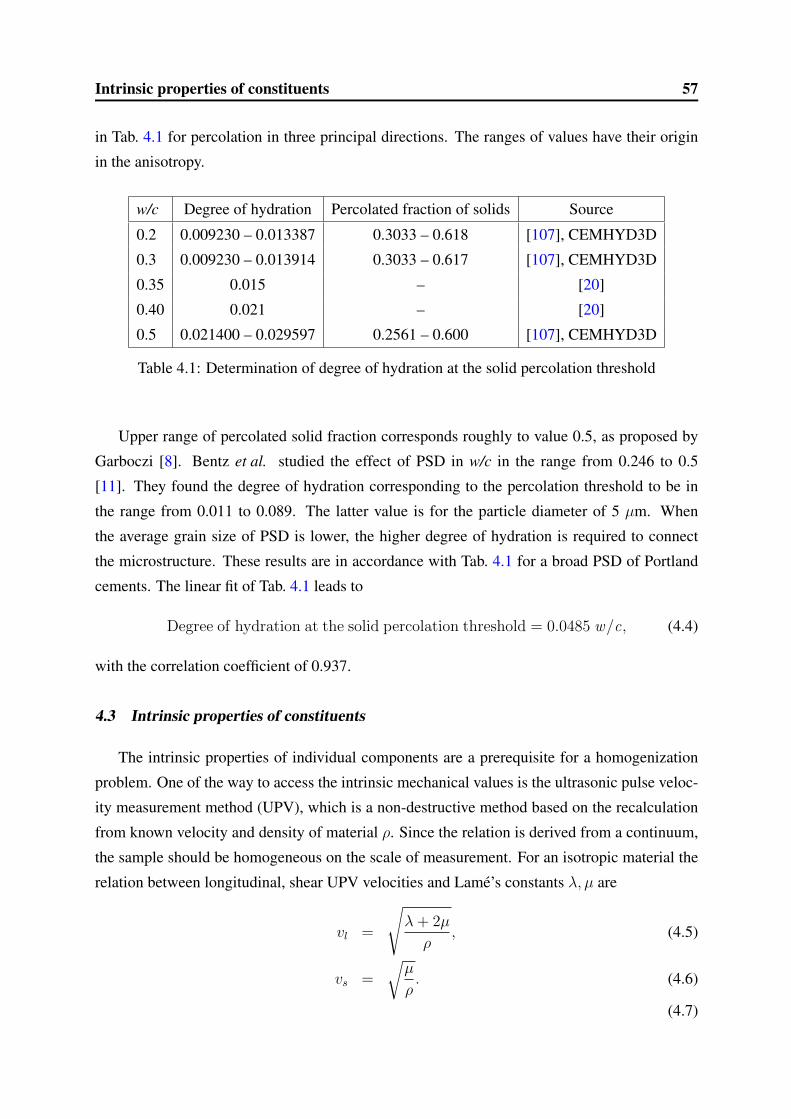
Intrinsic properties of constituents 57
in Tab. 4.1 for percolation in three principal directions. The ranges of values have their origin
in the anisotropy.
w/c Degree of hydration Percolated fraction of solids Source
0.2 0.009230 – 0.013387 0.3033 – 0.618 [107], CEMHYD3D
0.3 0.009230 – 0.013914 0.3033 – 0.617 [107], CEMHYD3D
0.35 0.015 – [20]
0.40 0.021 – [20]
0.5 0.021400 – 0.029597 0.2561 – 0.600 [107], CEMHYD3D
Table 4.1: Determination of degree of hydration at the solid percolation threshold
Upper range of percolated solid fraction corresponds roughly to value 0.5, as proposed by
Garboczi [8]. Bentz et al. studied the effect of PSD in w/c in the range from 0.246 to 0.5
[11]. They found the degree of hydration corresponding to the percolation threshold to be in
the range from 0.011 to 0.089. The latter value is for the particle diameter of 5 µm. When
the average grain size of PSD is lower, the higher degree of hydration is required to connect
the microstructure. These results are in accordance with Tab. 4.1 for a broad PSD of Portland
cements. The linear fit of Tab. 4.1 leads to
Degree of hydration at the solid percolation threshold = 0.0485 w/c, (4.4)
with the correlation coefficient of 0.937.
4.3 Intrinsic properties of constituents
The intrinsic properties of individual components are a prerequisite for a homogenization
problem. One of the way to access the intrinsic mechanical values is the ultrasonic pulse veloc-
ity measurement method (UPV), which is a non-destructive method based on the recalculation
from known velocity and density of material ρ. Since the relation is derived from a continuum,
the sample should be homogeneous on the scale of measurement. For an isotropic material the
relation between longitudinal, shear UPV velocities and Lame’s constants λ, µ are
vl =
√λ + 2µ
ρ, (4.5)
vs =
õ
ρ. (4.6)
(4.7)

Intrinsic properties of constituents 58
The elastic properties obtained from UPV experiments are often called dynamic moduli and
according to [62], the dynamic E modulus is higher than the static one for concrete probably
due to short-term creep [4]. The ratio Edyn/Estat varies from 1.5 to 1.7 for equivalent concrete
ages greater than 50 h. It is often found that the dependence of both moduli is almost linear
with the degree of hydration [62]. Above the hydration degree of 0.4, the rate of grow might
be lower. The extrapolation of elastic properties to early ages might be misleading, e.g. linear
extrapolation of the origin of static modulus points to the degree of hydration of 0.05, but yields
degree of hydration of 0.20 by a quadratic extrapolation for the same concrete [62]. Mind-
ness [73] and Nagy [78] also found that UPV provides usually a higher modulus of elasticity up
to 30 % than that determined by high strain static testing, e.g. ASTM C597. Therefore, these
non-destructive techniques are not generally recommended in practice but are very valuable in
modeling. The difference is partially attributed to a short-term creep phenomenon, especially
to C-S-H phases [4].
4.3.1 C-S-H mechanical properties
The C-S-H phases are intimately mixed with porosity and small CH crystals hence the re-
sults are sensitive to a selection of the cement paste region. Constantinides and Ulm [24] per-
formed a set of nanoindentation tests on OPC, w/c = 0.5, and they obtained data in Fig. 4.3.
They concluded that there are two types of C-S-H, assigning them properties in terms of Young’s
modulus: C-S-HLD ∼ 21.7± 2 GPa and C-S-HHD ∼ 29.4± 2.4 GPa. Poisson ratio was deter-
mined as 0.24 for both types. Acker [1] measured intrinsic properties of both types of C-S-H
with the results of 20 ± 2 GPa and 31 ± 4 GPa.
Figure 4.3: C-S-H nanoindentation data, w/c = 0.5, after [24]

Intrinsic properties of constituents 59
The C-S-H experimental results may be explained using the J-T model, where both C-S-H
forms are constructed from the same building unit [113]. According to the J-T model, two gel
porosities for C-S-HLD and C-S-HHD are 0.42 and 0.3, respectively. When the nanoindentation
results are correct, the homogenization at the C-S-H level from the building units would pre-
dict similar results. Unknown elastic properties of building units may be found with an inverse
homogenization problem. Indeed, the C-S-H morphology resembles a matrix-inclusion assem-
blage. Therefore the analytical Mori-Tanaka [75] homogenization theory may be applied with
the reference medium of C-S-HLD (C-S-HLD as a matrix with spherical porous inclusions). In
addition, the self-consistent scheme is checked without any reference phase. Tab. 4.2 summa-
rizes intrinsic values and downscaled intrinsic values using both schemes for the building units.
The independent nanoindentation results of both morphologies yielded nearly the same stiffness
of solid building units via the Mori-Tanaka scheme. This coincidence suggests that nanoinden-
tation, J-T model and the Mori-Tanaka scheme captures a true behavior. If so, the data from
porosimetry may be used to reconstruct the C-S-H structure and to predict its mechanical be-
havior.
C-S-H nanoindentation Porosity (J-T) Building units
Fraction in C-S-HLD - 0.42 0.58
Young’s modulus, E 21.7 GPa 0.001 53.22 - MT (137.4-SCS)
Poisson’s ratio, ν 0.24 0.001 (0.499) 0.265 - MT (0.37-SCS)
Fraction in C-S-HHD - 0.30 0.70
Young’s modulus, E 29.4 GPa 0.001 54.69 - MT (73.77 - SCS)
Poisson’s ratio, ν 0.24 0.001 (0.499) 0.257 - MT (0.277 - SCS)
Table 4.2: Downscaling of C-S-HLD and C-S-HHD to the building units using Mori-Tanaka and
self-consistent scheme
4.3.2 Cement paste level
The intrinsic elastic properties of cement paste level are important especially for unhydrated
clinker minerals and portlandite. Characteristic porosity of a phase is included in intrinsic prop-
erties. However, little data is available on the intrinsic porosity of raw cement clinker. Theisen
and Smidth [111] report porosity from 5 up to 25 vol. % for alite and belite, but including void
pores in epoxy resin.
Velez et al. [123] measured the elastic values of clinker minerals as they appear in Port-
land cement by nanoindentation and by means of the resonance frequency. They verified that

Intrinsic properties of constituents 60
there is no creep at constant force and low scatter of nanoindentation values. Poisson’s ratio is
assumed to be of 0.3 for all clinker minerals. Intrinsic data of CH were measured by several
researchers [1, 5, 128], see [17] for comprehensive results.
Phase E (nanoind.) ν E (resonance) Porosity [%] Ref.
(mechanical)
C3S 135±7 0.3 147±5 - [123]
C2S 130±20 0.3 140±10 - [123]
C3A 145±10 0.3 160±10 - [123]
C4AF 125±25 0.3 - - [123]
CSH2 16-30-35 0.18-0.3-0.34 - 3.5–7.5 [7]
Porositya 10−3 0.499924 - - -
10−3 10−3 - - -
CH 38±5 0.305-0.325 - - [24]
C-S-HLD 21.7±2.2 0.24 - - [24]
C-S-HHD 29.4±2.4 0.24 - - [24]
C6AS3H32 22.4 0.25 - - [57]
C4ASH12 42.3 0.324 - - [57]
C3AH6 22.4 0.25 - - *
FH3 22.4 0.25 - - *
Table 4.3: Intrinsic elastic moduli of chemical phases as measured by nanoindentation, reso-
nance frequency or mechanical tests. The Young moduli E with the standard deviation or range
are in GPa. Bold values are used in homogenization, * values are estimated, based on [57], a is
the water-filled porosity or the void, see further discussion
The study of portlandite crystal revealed that its structure is in the form of a trigonal lattice.
For such topographical configuration, linear elastic analysis based on density functional theory
was performed [65]. Six independent constants may be used for the reconstruction of stiffness
tensor. The global minimum value of Young’s modulus is 22.56 GPa when the angle between c-
axis of crystal and the direction of deformation is 39.82. The global maximum has the modulus
of 99.39 GPa in the perpendicular direction to c-axis. The stiffness tensor of portlandite has the

Intrinsic properties of constituents 61
following structure and numerically equals to [65]
Cij =
c11 c12 c13 c14 0 0
c12 c11 c13 −c14 0 0
c13 c13 c33 0 0 0
c14 −c14 0 c44 0 0
0 0 0 0 c44 |c14|0 0 0 0 |c14| 1
2(c11 − c12)
=
99.39 30.78 7.36 0 0 0
30.78 99.39 7.36 0 0 0
7.36 7.36 36.29 0 0 0
0 0 0 7.88 0 0
0 0 0 0 7.88 0
0 0 0 0 0 34.31
. (4.8)
The porosity presents a serious problem in the homogenization since it is in fact not a solid
phase. There are two types of porosities in the CEMHYD3D model; a water-filled porosity
and an empty porosity. While the water-filled porosity originates from mix water, the empty
porosity appears due to the depletion of water for hydration.
The elastic properties of water strongly influence the results for an early hydration period,
especially of Poisson’s ratio [17]. The water in the RVE cannot move freely out which is in
contradiction with the real cement paste at the beginning of hydration, especially during the
mechanical testing and resembles the problem of a saturated soil consolidation. If the water
movement is not restricted, the water should act in the micromechanical model as a void to
enable the compression.
Since presented analytical homogenization methods do not consider implicitly the deper-
colation of pore space, the water might be considered as a void so the percolation threshold
remains at 50 % of porosity of the self-consistent scheme. The Poisson ratio will then increase
during the whole hydration as the consequence of chosen water properties. Giving the water
its real elastic properties results in the decrease of Poisson’s ratio from the value of 0.5, on the
other hand, the percolation threshold of the self-consistence scheme is higher than 50 % of the
water-filled porosity.
In the numerical homogenization, the water-filled pores can have the bulk modulus of water
(k = 2.18 GPa) since the microstructure contains information about the connectivity of pores
and the strain may localize in empty pores. The next consequence of chosen porosity properties
is the speed convergence of FEM and FFT-based numerical homogenization methods since the
selection determines the contrast of phases.

Analytical homogenization methods 62
Chapter 5
ANALYTICAL HOMOGENIZATION METHODS
The methods of continuum mechanics relate the linear and nonlinear behavior at the funda-
mental level (phase or single crystal) with the macroscopic scale. Finding the effective physical
properties of composites is a classical engineering problem, where the domains of a heteroge-
neous material have different properties. The domain size is much larger than the molecular
dimensions and smaller than the macroscopic sample so these length scales can be viewed as
a continuum, Eq. (4.1). Empirical relations were found good for data correlation rather than
for prediction [116]. The microstructure configuration determines the effective properties in
addition to the volumetric fractions of the material domains. The most important, but not the
only one, is the volume fraction, or the result of one point autocorrelation function.
The continuum mechanics rely on the concept of concentration which is able to derive the
local stress or strain fields σ(x), ε(x) from the macroscopic ones Σ and E. This problem
cannot be solved in general, so additional assumption is made which leads to an estimate or to
a bound. In the case of estimates, the boundary conditions of inclusion are generally unknown,
so the problem is firstly transformed to the problem with homogeneous boundary conditions
[43, 51]. In the case of stress homogeneous boundary condition
p(x) = Σn, (5.1)
where n is the unit outward at the boundary and p are surface tractions. For any equilibrated
stress filed σ(x), the volume average yields back the homogeneous stress
〈σ〉 =1
V
∫V
σ(x)dV = Σ. (5.2)
Similarly a macroscopic strain can be imposed through surface displacements, which is
referred to as Hashin-type boundary condition
u(x) = Ex, (5.3)
where u(x) is microscopic displacement vector and x determines its position. For any strain
field ε(x) derived from any compatible displacement field according to Eq. (5.3), the macro-
scopic strain then reads
〈ε〉 =1
V
∫V
ε(x)dV = E. (5.4)

Analytical homogenization methods 63
The homogeneous boundary conditions according to Eqs. (5.1), (5.3) enable to use the Hill
lemma for the strain energy density, where at least strain or stress field satisfies homogeneous
boundary conditions
〈σ(x) : ε(x)〉 = 〈σ(x)〉 : 〈ε(x)〉 = Σ : E. (5.5)
The conditions of validity of Eq. (5.5) may be extended to periodic boundary conditions as
well [133]. In continuum micromechanics, the approximate microscopic stress or strain field
may be linked to the macroscopic one by means of strain A(x) or stress B(x) localization
(concentration) tensors in the case of linear elasticity
ε(x) = A(x) : E, (5.6)
σ(x) = B(x) : Σ. (5.7)
Eqs. (5.2), (5.4) imply that
〈A(x)〉 = 〈B(x)〉 = I. (5.8)
Combining Eq. (5.5) with Eqs. (5.4), (5.6) and subsequently with Eqs. (5.2), (5.7) yields
E : Σ = 〈ε(x) : σ(x)〉 = 〈ε(x) : B(x) : Σ〉, (5.9)
Σ : E = 〈σ(x) : ε(x)〉 = 〈σ(x) : A(x) : E〉. (5.10)
Eqs. (5.9), (5.10) lead to the same results in heterogeneous materials only in sufficiently
large samples. If not so, which is usually the case of representation in numerical analysis,
the results may be far apart and depend on boundary conditions [58]. This is discussed in
section 6.3. Let us define local constitutive equations (relating average microscopic strain with
stress at microscopic level)
σ(x) = c(x) : ε(x), (5.11)
ε(x) = s(x) : σ(x), (5.12)
where c(x) and s(x) are the local stiffness and compliance tensors, respectively.
Inserting Eq. (5.6) into Eqs. (5.11), (5.2) and Eq. (5.7) into Eqs. (5.12), (5.4) leads to the
effective stiffness and compliance tensors. Since a heterogeneous sample is often formed from
r phases with fr volume fractions, it is possible to replace integral with a summation
Σ = 〈σ〉 =1
V
∫V
cr : Ar : E dV =∑
r
frcr : Ar : E = Ceff : E, (5.13)
E = 〈ε〉 =1
V
∫V
sr : Br : Σ dV =∑
r
frsr : Br : Σ = Seff : Σ. (5.14)

Analytical homogenization methods 64
Following Eshelby’s idea [31], an estimate for the concentration tensor Aestr is obtained
from the solution of matrix-inclusion problem. If an inclusion has a spherical or ellipsoidal
shape and is embedded in a reference medium with the stiffness tensor C0, the strain field εr
in the inclusion is uniform from far imposed homogeneous strain. Such approach leads to an
estimate of elastic properties. The most common choice for localization tensor is the Eshelbian
type ellipsoidal inclusion placed in a reference medium [133]
Aestr =
[I + SEsh
r :(C−1
0 : cr − I)]−1
:
⟨[I + SEsh
r :(C−1
0 : cr − I)]−1
⟩−1
. (5.15)
The Eshelby tensor SEshr depends on the geometry and phase orientation. During the next
analysis, this tensor is considered to be of spherical inclusion type in isotropic media since the
cement paste resembles this type of morphology [17]. The Eshelby tensor is then composed of
volumetric and deviatoric parts
SEshr = α0J + β0K, (5.16)
α0 =3k0
3k0 + 4µ0
, (5.17)
β0 =6k0 + 12µ0
15k0 + 20µ0
, (5.18)
where k0, µ0 are the bulk and shear moduli of a reference medium and J, K are the volumetric
and deviatoric parts of a unity tensor I: Jijkl = (1/3) δijδkl and K = I - J, where δij represents
the Kronecker delta. Similarly, the stiffness tensor of the reference phase may be decomposed
Cr = 3krJ + 2µrK. (5.19)
The following relations between the elastic constants of the isotropic material are useful
when constructing the stiffness tensor from the Young modulus and the Poisson ratio
E =9kµ
3k + µ, (5.20)
ν =3k − 2µ
6k + 2µ, (5.21)
k =E
3(1− 2ν), (5.22)
µ =E
2(1 + ν). (5.23)

Hashin-Shtrikman and Walpole bounds 65
5.1 Rule of mixtures
The rule of mixtures is the first known micromechanical model, stated by Voigt in 1887.
It corresponds to a parallel alignment of phases where the localization tensor is estimated as
A = I
k =∑
i
kifi, (5.24)
µ =∑
i
µifi, (5.25)
where k is the bulk modulus, µ the shear modulus and f the volume fraction of individual
phases. In the case of serial alignment and perfect bonding, the Reuss estimation with B = I is
recovered1
k=
∑i
fi
ki
, (5.26)
1
µ=
∑i
fi
µi
. (5.27)
Although seeming as an oversimplification, the rules of mixture yield the bounds that can-
not be exceeded in the case of elastic isotropic material by any other homogenization method.
Fig. 7.4 gives an example of upper bound in a real hydrating cement paste.
5.2 Hashin-Shtrikman and Walpole bounds
Hashin and Shtrikman bounds (HS), elaborated in 1962, provide the estimate of bounds
for elastic constants in the heterogeneous material [44]. The necessary condition, under these
bound were derived, is a random isotropic distribution of phases and the same order of elastic
moduli k and µ, i.e. both have to increase or decrease for all phases simultaneously.
HS bounds are very useful for a rapid checking of heterogeneous materials if they satisfy
conditions of phase random distribution and moduli order. On the other hand, if the experi-
mental effective properties lie bellow the lower HS bound, a discontinuous behavior is to be
expected, in the forms of defects or cracks. Hashin-Shtrikman bounds are much narrower than
Voigt-Reuss bounds since additional information about random isotropic distribution is taken
into account.
Hashin and Shtrikman [44] found that the lower bound of bulk modulus coincides with the
effective bulk modulus of coated sphere assemblage as discussed in section 5.5. When the
phases of coated spheres are interchanged, the effective bulk modulus corresponds to the upper
Hashin-Shtrikman bound. The reason of bounds coincidence is in spherical symmetry, which
substitutes isotropic material, and exhibits the constant strain field within one phase.

Mori-Tanaka method 66
HS bounds coincide with the scheme of Mori and Tanaka in the case that composite matrix
is made from the softer phase and inclusions are in the form of spheres, or randomly distributed
ellipsoids. However, the results are not equal in case of elongated particles with different shapes
or orientations.
Consider a two phase medium with bulk moduli k1, k2, shear moduli µ1, µ2, and phase
fractions f1, f2. Suppose the following inequalities for both phases
k1 ≤ k2, µ1 ≤ µ2. (5.28)
The resulting elastic bounds of Hashin-Shtrikman are calculated from a variational formulation
k1 +f2
1k2−k1
+ 3f1
3k1+4µ1
≤ keff ≤ k2 +f1
1k1−k2
+ 3f2
3k2+4µ2
, (5.29)
µ1 +f2
1µ2−µ1
+ 6f1(k1+2µ1)5µ1(3k1+4µ1)
≤ µeff ≤ µ2 +f1
1µ1−µ2
+ 6f2(k2+2µ2)5µ2(3k2+4µ2)
. (5.30)
If more phases are present in a composite, the necessary order of bulk and shear moduli are
of importance. The phases must have increasing or decreasing bulk and shear moduli together.
If not so, Walpole or Hashin-Shtrikman-Walpole broader bounds should be used [18]. The
resulting formula for bulk and shear modulus bounds of the latter reads
khighlow =
⟨ 1
kr + 43µmax
min
⟩−1
− 4
3µmax
min =
(∑r
fr
kr + 43µmax
min
)−1
− 4
3µmax
min , (5.31)
µhighlow =
⟨ 1
µr + kmaxmin
⟩−1
− kmaxmin =
(∑r
fr
µr + kmaxmin
)−1
− kmaxmin , (5.32)
where kmaxmin and µmax
min are maximal and minimal absolute values of the bulk and shear moduli
in a composite and fr are the volume fractions of phases. An example of applied bounds is in
Fig. 7.4. The bounds are usually wide for porous materials and for practical evaluation are of
little importance.
5.3 Mori-Tanaka method
The Mori-Tanaka homogenization method [75] assumes a matrix-inclusion morphology of
considered phases, as derived in terms of localization in Eq. (5.15) and extended to elliptical
pores, e.g. [98].
The Mori Tanaka scheme for estimating the effective moduli is applicable to regions of the
graded microstructure that have a well-defined continuous matrix and a discontinuous particu-
late phase as showed in Fig. 5.1. It takes into account the weak interaction of the elastic fields

Self-consistent scheme 67
Figure 5.1: Material with particulate struc-
tureFigure 5.2: Material with skeletal structure
between neighboring inclusions. The matrix phase, denoted as the reference phase and by sub-
script 0, is reinforced by spherical particles of a particulate phases, denoted by subscript r. In
this notation, k0, µ0 are the bulk and shear matrix moduli and kr, µr refer to phases that rep-
resent inclusions. The following explicit estimates are derived from Eq. (5.15) when inserting
Eq. (5.16) - (5.19). α0 and β0 are according to Eqs. (5.17), (5.18). The explicit results for the
effective bulk modulus k and the shear modulus µ then read
khom =
∑r frkr
(1 + α0
(kr
k0− 1))−1
∑r fr
(1 + α0
(kr
k0− 1))−1 , (5.33)
µhom =
∑r frµr
(1 + β0
(µr
µ0− 1))−1
∑r fr
(1 + β0
(µr
µ0− 1))−1 . (5.34)
5.4 Self-consistent scheme
The self-consistent scheme (SCS) of Budiansky, elaborated by Hill [51] is an implicit
scheme for composites with the skeletal structure in Fig. 5.2, incorporating the Eshelby tensor
and based on Eq. (5.15). Reference medium points to the homogenized medium itself hence the
solution is in implicit form. The iterative procedure may be rewritten from Eqs. (5.33), (5.34),
substituting k0 for khom and µ0 for µhom, respectively. In porous materials, the implicit formula-
tion yields elastic properties of porous phase when the porosity fraction is above approximately
50 %. Good results of the self-consistent scheme were reported on Voronoı cells with Young’s
moduli ratios of 1:100 and with the amount of up to 50 % of solid phase representation [58].

Self-consistent scheme 68
The threshold of SCS may be used to account for solid percolation threshold in cement
pastes [17]. Selection of elastic properties of capillary porosity determines the volume fraction
at which SCS yields the threshold. When porosity is considered with the elastic parameters
of water, Tab. 4.3, the SCS threshold needs more than 50 % of capillary water-filled porosity.
When the water-filled porosity is considered with a very low Poisson’s ratio, i.e. corresponding
to a true void, the SCS yields the threshold at exactly 50 % of porosity.
To demonstrate the performance of SCS in various w/c’s, the homogenization level of ce-
ment paste is carried out, Fig. 5.3. The intrinsic mechanical values from Tab. 4.3 are used, with
the water-filled porosity. The data of OPC are taken from Slamecka [107] and the relation-
ship between capillary porosity and Young’s modulus E from empirical formula according to
Eq. (7.1), [57].
0
5
10
15
20
25
30
35
40
45
50
0 0.1 0.2 0.3 0.4 0.5 0.6 0.7
E o
f pas
te [G
Pa]
Porosity [-]
0.20.30.5
46.03(1-p)3.16
Figure 5.3: Performance of self consistent scheme with and without solid percolation
When a Portland cement paste has w/c = 0.318, the set point coincides with 50 % of void
porosity which is the threshold of self-consistent scheme [17]. If the w/c is lower, the paste
exhibits non-negligible Young’s modulus right from the beginning of hydration, which is the
problem of particle contact and assumption of perfect bonding in homogenization problem.
The solid percolation threshold pc from where the cement paste should exhibit mechanical
response, was determined by CEMHYD3D model as the first non-zero value in any of three
principal directions accounted for solid percolation. The results of pc are similar to Tab. 4.1.
Eq. (1.2) was modified to account for percolation in the simplest way. It was assumed that the
same amount of phases exist in the percolated path and in the rest of the phases, arriving to a
proportional relation with percolated fraction
Eperc = ESCSp− pc
1− pc
, (5.35)

N-layered spheres 69
where Eperc is the corrected ESCS modulus for the percolation of solids. Indeed, the reduced
Young modulus is then closer to experimental fit in Fig. 5.3. For high w/c, the percolation
is much less significant than in the case of low w/c, Fig. 5.3. Another way to account for
percolation is to filter directly the RVE which will result in modified volume fractions while
satisfying the assumption of perfect bonding among phases.
Another example is an uncoupling of length scales via the SCS, Tab. 5.1. Three phases are
considered, A as a solid phase and B, C as the water-filled porosity. The homogenization order
will be altered to show how these levels are associated. Homogenization ”all at one” generally
gives the lowest values, line 10 in Tab. 5.1, since the nominator in Eqs. (5.33), (5.34) is the
lowest due to the fact that kB and kC are nearly zero. The line 7 reflects the arrangement,
where the phase A has an intrinsic porosity B and this mixture as one phase is inserted in the
porous phase C. Therefore, the porosity distributed over different length scales does not reduce
effective properties so considerably as the porosity at one scale in the same volume.
Line Phase Vol. fraction E ν k µ
1 A 0.63 10 0.3 8.333 3.846
2 B 0.07 10−6 0.49 0.000 0.000
3 C 0.30 10−6 0.49 0.000 0.000
4 A+C 0.677 : 0.323 3.531 0.247 2.329 1.416
5 B+C 0.189 : 0.811 10−6 0.49 0.000 0.000
6 A+B 0.9 : 0.1 7.995 0.287 6.244 3.107
7 (A+B)+C (0.7) : 0.3 3.185 0.245 2.083 1.279
8 A+(B+C) 0.63 : (0.37) 2.583 0.236 1.634 1.045
9 (A+C)+B (0.93) : 0.07 3.036 0.243 1.969 1.221
10 A+B+C 0.63 : 0.07 : 0.3 2.583 0.236 1.634 1.045
Table 5.1: Homogenization with different phase order on a three phase system
5.5 N-layered spheres
Herve and Zaoui [47] derived elastic strains and stresses of n-layered isotropic spherical
inclusions embedded in an unbounded matrix. The uniform stress or strain load is applied in
infinity. Continuity of displacements and stresses is assumed between adjacent spheres. Similar
models of spherical assemblages and isotropic elasticity were derived by Hashin [43] or Chris-
tensen and Lo [23] for two material phases in the form of two isotropic spheres. The n-layered

Other elastic homogenization models 70
model may be extended to arbitrary number of phases embedded in an infinite homogenized
medium. The geometrical representation of the Herve-Zaoui scheme is in Fig. 5.4.
13 R1
R
R
2
3
2
n+1
hom. medium
n
Figure 5.4: The geometrical representation of the 3-layered Herve-Zaoui scheme
There are two possible applications of the Herve and Zaoui scheme: the first one taking
n + 1 phases, i.e. also the elastic properties of the homogenized medium. The resulting dis-
placements and stresses may be calculated. The second application of the scheme is the deter-
mination of homogeneous elastic medium around the spherical inclusions, taking only elastic
properties of n isotropic phases. The derivation of Herve and Zaoui scheme is in Appendix A.
It must be emphasized that in the case of two spherical inclusions, i.e. n = 2, the scheme
provides the same estimates as the Hashin-Shtrikman bounds. If the bulk and shear moduli are
in an ascending order from the center, i.e. the core is more compliant than the shell, then the
result coincide with the upper Hashin-Shtrikman bound. In the reversed configuration, i.e. the
cherry-pit model, the lower Hashin-Shtrikman bound is found [47].
Heutkamp and Ulm [48] used this scheme for the study of ITZ in leached cement pastes.
The order of phases according to Fig. 5.4 was the following; 1 = sand, 2 = ITZ, 3 = cement
paste, hom. medium = mortar. They found a reduction of Young’s modulus of degraded cement
paste by 40 or 45 % in ITZ. In their case, the ITZ thickness was assumed as 20 µm. The Herve
and Zaoui scheme will be validated for the effect of ITZ in section 7.3.
5.6 Other elastic homogenization models
Beyond presented homogenization models, other models applied directly to concrete were
derived as well [71]. Hirsch combined Voigt and Reuss models, disregarding lateral deforma-
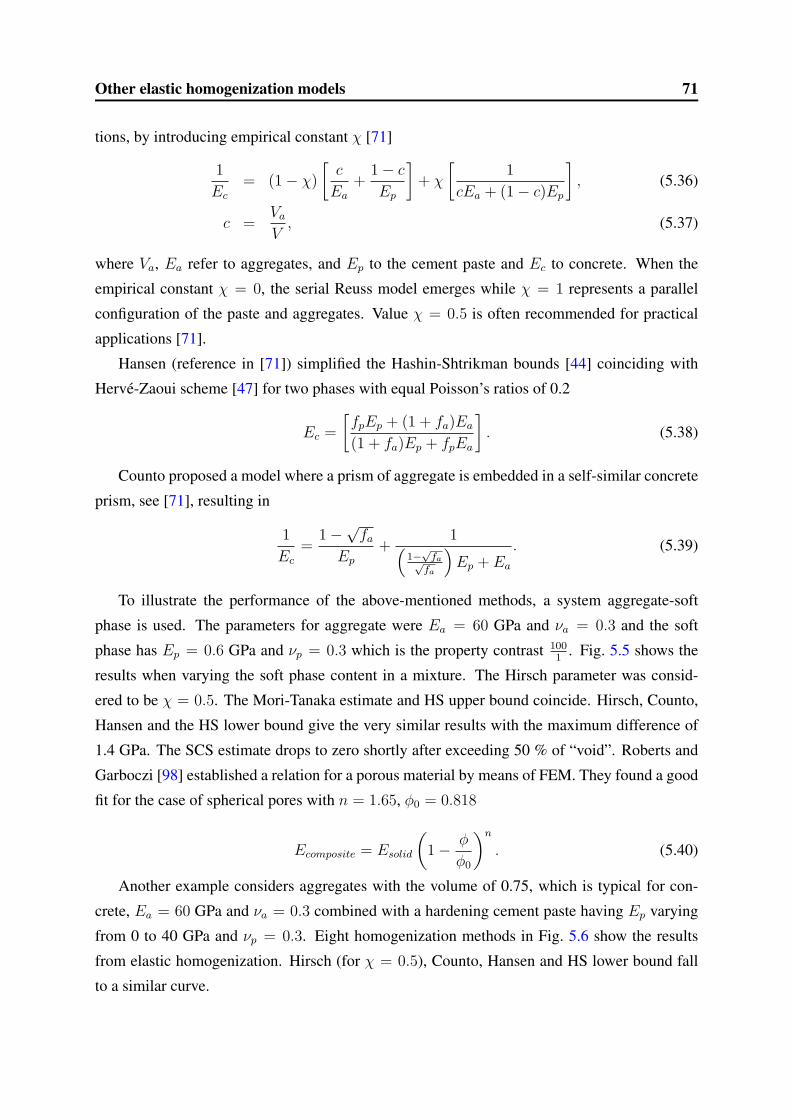
Other elastic homogenization models 71
tions, by introducing empirical constant χ [71]
1
Ec
= (1− χ)
[c
Ea
+1− c
Ep
]+ χ
[1
cEa + (1− c)Ep
], (5.36)
c =Va
V, (5.37)
where Va, Ea refer to aggregates, and Ep to the cement paste and Ec to concrete. When the
empirical constant χ = 0, the serial Reuss model emerges while χ = 1 represents a parallel
configuration of the paste and aggregates. Value χ = 0.5 is often recommended for practical
applications [71].
Hansen (reference in [71]) simplified the Hashin-Shtrikman bounds [44] coinciding with
Herve-Zaoui scheme [47] for two phases with equal Poisson’s ratios of 0.2
Ec =
[fpEp + (1 + fa)Ea
(1 + fa)Ep + fpEa
]. (5.38)
Counto proposed a model where a prism of aggregate is embedded in a self-similar concrete
prism, see [71], resulting in
1
Ec
=1−
√fa
Ep
+1(
1−√
fa√fa
)Ep + Ea
. (5.39)
To illustrate the performance of the above-mentioned methods, a system aggregate-soft
phase is used. The parameters for aggregate were Ea = 60 GPa and νa = 0.3 and the soft
phase has Ep = 0.6 GPa and νp = 0.3 which is the property contrast 1001
. Fig. 5.5 shows the
results when varying the soft phase content in a mixture. The Hirsch parameter was consid-
ered to be χ = 0.5. The Mori-Tanaka estimate and HS upper bound coincide. Hirsch, Counto,
Hansen and the HS lower bound give the very similar results with the maximum difference of
1.4 GPa. The SCS estimate drops to zero shortly after exceeding 50 % of “void”. Roberts and
Garboczi [98] established a relation for a porous material by means of FEM. They found a good
fit for the case of spherical pores with n = 1.65, φ0 = 0.818
Ecomposite = Esolid
(1− φ
φ0
)n
. (5.40)
Another example considers aggregates with the volume of 0.75, which is typical for con-
crete, Ea = 60 GPa and νa = 0.3 combined with a hardening cement paste having Ep varying
from 0 to 40 GPa and νp = 0.3. Eight homogenization methods in Fig. 5.6 show the results
from elastic homogenization. Hirsch (for χ = 0.5), Counto, Hansen and HS lower bound fall
to a similar curve.

Other elastic homogenization models 72
0
10
20
30
40
50
60
0 0.2 0.4 0.6 0.8 1
E o
f con
cret
e [G
Pa]
Vol. amount of soft phase [-]
VoigtMori TanakaHS highFEMSCSHirschCountoHansenHS lowReuss
Figure 5.5: Homogenization of an aggregate with a soft phase
0
10
20
30
40
50
60
0 5 10 15 20 25 30 35 40
E o
f con
cret
e [G
Pa]
E of paste [GPa]
VoigtMori TanakaHashin highHirschCountoHansenHashin lowReuss
Figure 5.6: Homogenization of an aggregate with hydrating cement paste

General principles and material isotropy 73
Chapter 6
NUMERICAL HOMOGENIZATION METHODS
6.1 General principles and material isotropy
The aim of numerical homogenization methods is to find again an effective stiffness tensor
of the homogenized medium that would behave in the same way as a heterogeneous composite
on finite dimensions. The finite dimensions are represented with the RVE which is a sufficiently
large material sample to be statistically representative. The boundary conditions must be im-
posed on the RVE to define uniquely the homogenization problem. The numerical methods
are used to find a static equilibrium within the RVE associated with the boundary conditions.
Eqs. (5.2), (5.4) formulate stress and strain averages over the RVE and Eqs. (5.13), (5.14) the
effective homogenized stiffness and compliance tensors.
The homogenization method will be further restrained to isotropic intrinsic properties and it
is natural to expect a homogenized isotropic response due to the definition of the RVE. The 3D
constitutive equation in a tensorial form of isotropic homogeneous material may be rewritten in
the engineering matrix and vector notation
σxx
σyy
σzz
τxy
τyz
τzx
=
E
(1+ν)(1−2ν)
1− ν ν ν
ν 1− ν ν
ν ν 1− ν
0
0
µ 0 0
0 µ 0
0 0 µ
εxx
εyy
εzz
γxy(2ε12)
γyz(2ε23)
γxz(2ε13)
, (6.1)
where the shear modulus µ is defined in Eq. (5.23) and the Cauchy stress vector σ has the
components
σ = σ11, σ22, σ33, σ12, σ23, σ13T , (6.2)
and consequently the small strains vector ε
ε = ε11, ε22, ε33, 2ε12, 2ε23, 2ε13T . (6.3)
Anisotropy may appear in the RVE due to an insufficient size of the RVE, e.g. the perco-
lation at early ages. The principle of energy conservation was used for the transition from a

Eigenstrain method 74
generally anisotropic to an isotropic homogenized material. Isotropic material is characterized
by two independent constants, e.g. Young’s modulus and Poisson’s ratio. The stiffness matrix
of an isotropic material, Eq. (6.1), may be seen as two independent submatrices: the upper sub-
matrix 3× 3 relates the normal stresses and strains, while the lower submatrix 3× 3 relates the
shear stresses and strains. From these two submatrices and with the help of stored energy in an
anisotropic material, two independent elastic constants of isotropic medium may be calculated
in one step. The work in a unity of linear isotropic material reads
W =1
2εT σ =
1
2εT Ceffε. (6.4)
Eq. (6.4) leads to the following set of equations that finally yields the homogeneous Young’s
modulus and Poisson’s ratio ν, all in engineering terms
µ =γxyτxy + γyzτyz + γxzτxz
γ2xy + γ2
yz + γ2xz
, (6.5)
a = ε2xx + ε2
yy + ε2zz, (6.6)
b = 2(εxxεyy + εxxεzz + εyyεzz), (6.7)
Wn = εxxσxx + εyyσyy + εzzσzz, (6.8)
ν =Wu − µa
µ(b− a) + 2Wu
, (6.9)
E = 2µ(1 + ν), (6.10)
where Wn stores twice the amount of internal energy.
6.2 Eigenstrain method
Eigenstrain is a generic name of a stress-free strain that exists in a material due to former
history as welding, phase transformation, initial strains, plastic strains etc. One of good repre-
sentatives and the most common application of eigenstrains is temperature. Temperature is a
special kind of eigenstrain where the shear components equal to zero so only axial effects are
involved. The other names for eigenstrain as a stress-free strain or a polarization strain may
appear in the literature.
Similarly, an eigenstress is a self-equilibrated internal stress that was caused by eigenstrain
in bodies that are not loaded by any external force. The advantage of using eigenstrain is the
way of imposing of residual stresses in a linear model of elasticity. This method will be used
further as a loading condition that corresponds to a homogeneous strain state.
In the theory of small deformations, the total strain εij is considered as the sum of elastic
strain εelasij and eigenstrain εeigs
ij
εij = εelasij + εeigs
ij . (6.11)

Eigenstrain method 75
The total strain, which includes eigenstrain, is compatible with deformation
εij =1
2(ui,j + uj,i) . (6.12)
The stiffness tensor of material is symmetric thanks to Cauchy’s second law of motion,
which means that ui,j = uj,i. The constitutive equation for linear elastic material is corrected
for the effect of eigenstrain, by substituting Eqs. (6.11), (6.12)
σij = Cijklεkl = Cijkl
(εkl − εeigs
kl
), (6.13)
σij = Cijkl
(uk,l − εeigs
kl
). (6.14)
Let us compare two loading conditions: the first case will deal with an arbitrary and equi-
librated stress state on the domain. In the second case, only eigenstrain will be assumed while
the material domain will be free from any external forces and boundary constraints
σij,j = 0, ∀x ∈ Ω, (6.15)
σijnj = 0, ∀x ∈ Γ, (6.16)
where nj is the outer vector of the boundary. After substituting Eq. (6.14) into Eq. (6.15) and
Eq. (6.16), the following equations relating displacements and eigenstrains are obtained
Cijkluk,lj = Cijklεeigskl,j , ∀x ∈ Ω, (6.17)
Cijkluk,lnj = Cijklεeigskj nj, ∀x ∈ Γ. (6.18)
Eq. (6.17) proves that the contribution of eigenstrains can be replaced with a body forces
while Eq. (6.18) sets up the relationship between surface tractions and eigenstrains. The body
forces −Cijklεeigskj and the surface tractions Cijklε
eigskj nj create the same displacement field
across the domain.
In the case that only some part of the domain (such as any kind of inclusion) is loaded by the
eigenstrain, the equilibrium conditions on the surface Γi between inclusion and matrix follows
as in Eq. (6.17)
Cijkluk,lj + Cijklεeigskl,j χ(x) = 0, (6.19)
χ(x) = 1 ∀x ∈ Γi, otherwise 0, (6.20)
εeigskl,j = εeigs
kl nj. (6.21)
The solution of Eq. (6.19) for the given eigenstrain εeigskl is obtainable through the methods
of periodicity, such as Fourier series or Green’s function.
When imposing eigenstrains to the domain, the strains are introduced to all material phases
regardless of their intrinsic mechanical properties and the homogenized stiffness tensor does

Smaller volume then the representative volume element 76
not depend on imposed eigenstrain. Since the relation between strains, or eigenstrains, and
displacement exists, the body is then subjected to homogeneous displacement conditions over
the domain. For example, the periodic material yields the macroscopic stiffness tensor
Chom : E = Σ = 〈C(x) : (ε(u∗) + E)〉, (6.22)
where u∗ is a fluctuation part of the periodic displacement field. Input eigenstrains E may be
chosen arbitrarily resulting to the same Chom.
The above-mentioned strain approach may be substituted with a stress approach, prescribing
overall homogeneous stress for the domain. This topic is discussed in detail, e.g. [72, 134].
6.3 Smaller volume then the representative volume element
In every practical simulation, the RVE is smaller then the studied material sample. Huet [52]
coined the term apparent properties which results from an insufficient size of RVE. Two lim-
iting types of boundary conditions may be imposed on the RVE. The static uniform boundary
conditions (SUBC) are defined in such a way, that the tractions are prescribed on the boundary Γ
σn = Σn, ∀x ∈ Γ. (6.23)
On the other hand, kinematic uniform boundary conditions (KUBC) follow the prescribed
displacements on the boundary from the given strain E
u = Ex, ∀x ∈ Γ. (6.24)
The response of loading conditions according to Eqs. (6.23), (6.24) yields the same result
only when the size of RVE is large enough (compare with Eqs. (5.13), (5.14)). In such a particu-
lar case, the material macroscopic response is independent of the applied boundary conditions.
The special case of boundary conditions is the periodic one, which is always a combination
of the KUBC and SUBC. Huet [52] proved that SUBC and KUBC are the bounds of effec-
tive properties on insufficiently sized RVE, following the inequalities of apparent and effective
stiffness tensors
CappSUBC ≤ Capp
PERIODIC ≤ CappKUBC , (6.25)
CappSUBC ≤ Ceff ≤ Capp
KUBC , (6.26)
where Capp is the apparent stiffness fourth-order tensor. The inequality can be understood in the
sense of quadratic form, i.e., ε : C : ε for any tensor ε 6= 0. The same inequality works for bulk
and shear moduli but not for Young’s modulus or Poisson’s ratio. For the effect of boundary
condition type in real cement pastes, see Fig. 7.7.
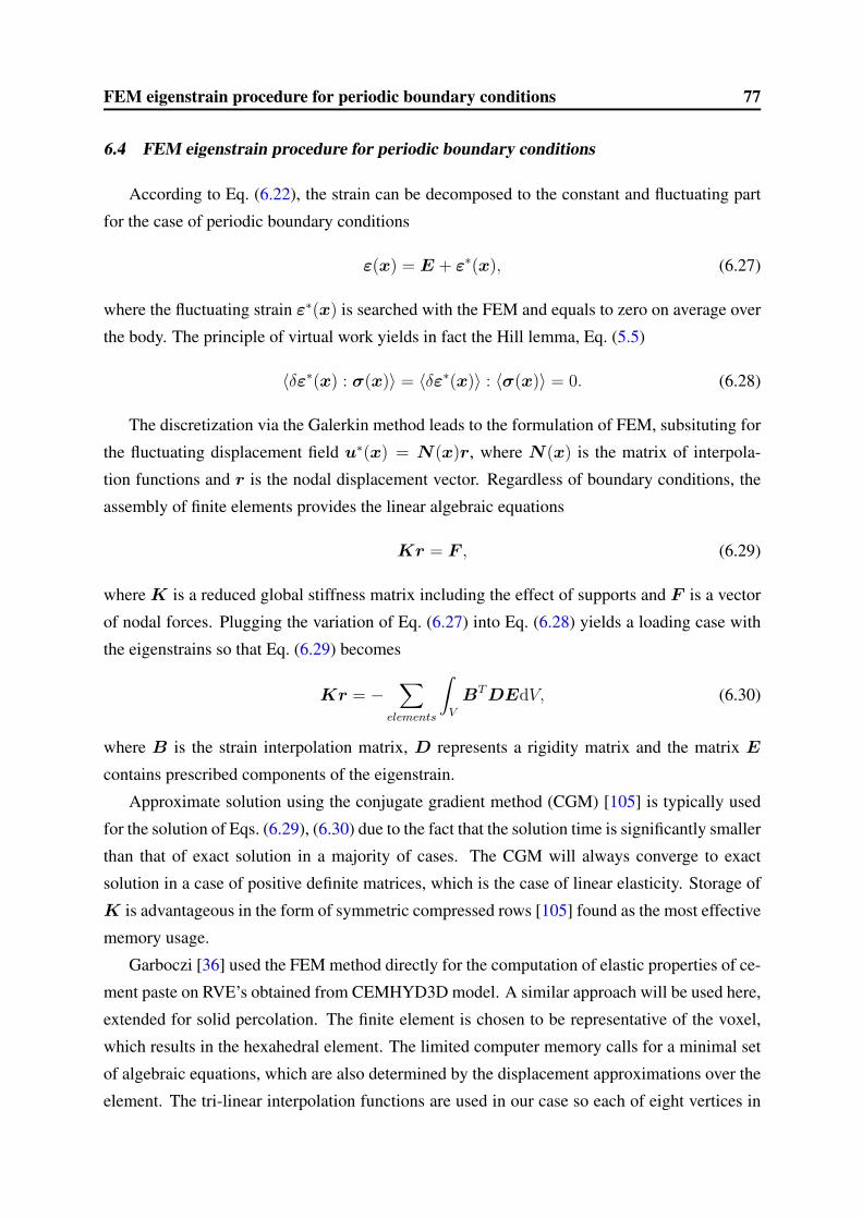
FEM eigenstrain procedure for periodic boundary conditions 77
6.4 FEM eigenstrain procedure for periodic boundary conditions
According to Eq. (6.22), the strain can be decomposed to the constant and fluctuating part
for the case of periodic boundary conditions
ε(x) = E + ε∗(x), (6.27)
where the fluctuating strain ε∗(x) is searched with the FEM and equals to zero on average over
the body. The principle of virtual work yields in fact the Hill lemma, Eq. (5.5)
〈δε∗(x) : σ(x)〉 = 〈δε∗(x)〉 : 〈σ(x)〉 = 0. (6.28)
The discretization via the Galerkin method leads to the formulation of FEM, subsituting for
the fluctuating displacement field u∗(x) = N (x)r, where N (x) is the matrix of interpola-
tion functions and r is the nodal displacement vector. Regardless of boundary conditions, the
assembly of finite elements provides the linear algebraic equations
Kr = F , (6.29)
where K is a reduced global stiffness matrix including the effect of supports and F is a vector
of nodal forces. Plugging the variation of Eq. (6.27) into Eq. (6.28) yields a loading case with
the eigenstrains so that Eq. (6.29) becomes
Kr = −∑
elements
∫V
BT DEdV, (6.30)
where B is the strain interpolation matrix, D represents a rigidity matrix and the matrix E
contains prescribed components of the eigenstrain.
Approximate solution using the conjugate gradient method (CGM) [105] is typically used
for the solution of Eqs. (6.29), (6.30) due to the fact that the solution time is significantly smaller
than that of exact solution in a majority of cases. The CGM will always converge to exact
solution in a case of positive definite matrices, which is the case of linear elasticity. Storage of
K is advantageous in the form of symmetric compressed rows [105] found as the most effective
memory usage.
Garboczi [36] used the FEM method directly for the computation of elastic properties of ce-
ment paste on RVE’s obtained from CEMHYD3D model. A similar approach will be used here,
extended for solid percolation. The finite element is chosen to be representative of the voxel,
which results in the hexahedral element. The limited computer memory calls for a minimal set
of algebraic equations, which are also determined by the displacement approximations over the
element. The tri-linear interpolation functions are used in our case so each of eight vertices in

FEM eigenstrain procedure for periodic boundary conditions 78
1
2
322
33
3
3 3
3
Figure 6.1: FEM implementation of voxelized microstructure with periodic boundary con-
ditions
the hexahedral (brick) element has three DOF’s. The microstructure yields a structured regular
mesh that may be easily generated without the need of external mesh generator, Fig. 6.1.
Suppose that the heterogeneous domain with the periodic boundary conditions is subjected
to an uniform eigenstrain. The force contributions from the adjacent finite elements are intro-
duced to the nodes. In the case of linear elasticity, solving the linear equations provides the
unknown nodal displacements. Since the stresses are in principle discontinuous due to hetero-
geneous materials, volume averaging of strains and stresses is performed via integration points
on elements according to Eq. (5.5). When a homogeneous strain is applied to the heterogeneous
RVE, the average strain equals back to the input strain.
Periodic boundary conditions on RVE may be effectively implemented by a code number
technique [59]. The advantage of this method is no increase of degrees of freedom or additional
parameters like in the case of penalty method, e.g. [134]. On the other hand, the bandwidth of
stiffness matrix increases which slows down the consecutive elimination.
Fig. 6.1 shows a typical situation for the RVE with the periodic boundary conditions. Each
node on the RVE side experiences the same periodic displacement as the opposite node (num-
ber 1) so they are denoted as virtual pairs. Particular node on the edge of the RVE has three
virtual twins (number 2) and each vertex node has seven virtual twins (number 3). These rela-
tions are simply expressed in terms of identical nodal code numbers. Support of microstructure
is chosen as fixed displacements in one vertex (number 3) so all eight vertices are fixed.

FEM eigenstrain procedure for periodic boundary conditions 79
6.4.1 Numerical verification
The first set of verifications is carried out on a simple microstructure consisting of two
phases. A checkerboard symmetrical configuration allows to use directly the hexahedral ele-
ments, Fig. 6.2. The periodic boundary conditions with eigenstrain load are assumed. When
the RVE size is 2 × 2 × 2 then there is no nodal displacement at vertices at all. This allows
checking directly the performance of element due to imposed eigenstrain. The regular mesh
refinement improves the results, which converge to the correct solution. The results for hexa-
hedral element with tri-linear shape function are summarized in Tab. 6.1. Eq. (6.30) was solved
with the LDL decomposition [105]. The phase mechanical parameters are chosen in such a
way that the shear moduli are equal [36]. In such a particular case, equal shear moduli must be
obtained, regardless of morphology in 2D or 3D, leading to the homogenized bulk moduli in
2D or 3D
k2D =µ(c1k1 + c2k2) + k1k2
µ + c1k2 + c2k1
, (6.31)
k3D =43µ(c1k1 + c2k2) + k1k2
43µ + c1k2 + c2k1
, (6.32)
where µ is the equal shear modulus, k1, k2 are bulk moduli of two phases, k2D, k3D are the
resulting bulk moduli and c1, c2 are volumetric fractions. Fig. 6.2 displays the mesh and nodal
displacement on three mesh refinements. Note that the edges on the periodic unit cell remain
straight since coupling of opposite twin nodes creates the periodic RVE.
- Phase 1 Phase 2 8 elmts 64 elmts 1000 elmts Exact
E 2.25 2.95082 2.907 2.826 2.732 2.688ν 0.125 0.47541 0.454 0.413 0.366 0.344k3D 1.0 20 10.50 5.438 3.399 2.873
µ 1.0 1.0 1.0 1.0 1.0 1.0
c1 - - 0.5 0.5 0.5 0.5
c2 - - 0.5 0.5 0.5 0.5
DOF’s - - 21 189 2997 -
Time [s] - - 0.23 1.11 51.00 -
Table 6.1: FEM results from checkerboard configuration on hexahedral elements with linearapproximations and consumed CPU time (400 MHz, LDL solver)
In order to get better results, quadratic approximation functions are used for the approxi-
mation of displacements. Hence, quadratic hexahedral element with 20 nodes and 60 DOF’s is

FEM eigenstrain procedure for periodic boundary conditions 80
a) 2 × 2 × 2 b) 4 × 4 × 4 c) 10 × 10 × 10
Figure 6.2: Displacements on checkerboard structure using linear hexahedral element
used in the 3D analysis. The same microstructure with identical input values was checked for
performance, Fig. 6.3 and Tab. 6.2.
- Phase 1 Phase 2 8 elmts 64 elmts 216 elmts 1000 elmts Exact
E 2.25 2.95082 2.908 2.745 2.722 2.703 2.688ν 0.125 0.47541 0.454 0.373 0.361 0.351 0.344k3D 1.0 20 10.50 3.596 3.266 3.032 2.873
µ 1.0 1.0 1.0 1.0 1.0 1.0 1.0
c1 - - 0.5 0.5 0.5 0.5 0.5
c2 - - 0.5 0.5 0.5 0.5 0.5
DOF’s - - 93 765 2589 11997 -
Time [s] - - 3.4 18.50 105 32 min. -
Table 6.2: FEM results from checkerboard configuration on hexahedral elements with
quadratic approximations and consumed CPU time (400 MHz, LDL solver)
The second set of examples will deal with unpercolated cement paste microstructures and
will briefly discuss the results. The microstructure of original 25 × 25 × 25 µm size for the
Kamali et al. ’s experiments is used [57], see section 7.1.2 and 7.1.3, and increased two and
three times which corresponds to a finer resolution. Two microstructures are used: the dense
one with w/c = 0.25 and the looser one with w/c = 0.5. The evolution of modulus of elasticity
is depicted in Figs. 6.4, 6.5. Capillary porosity is considered as a water-filled one.
Generally, FEM overestimates modulus of elasticity due to coarse approximations of dis-
placements. The FEM results, in terms of Young’s modulus, are very close to the linear re-

FEM eigenstrain procedure for periodic boundary conditions 81
a) 2 × 2 × 2 b) 4 × 4 × 4 c) 10 × 10 × 10
Figure 6.3: Displacements on checkerboard structure using quadratic hexahedral element
0
5
10
15
20
0 0.1 0.2 0.3 0.4 0.5 0.6 0.7 0.8 0.9
You
ng’s
mod
ulus
, E [G
Pa]
Degree of hydration [-]
25 x 25 x 2550 x 50 x 5075 x 75 x 75
0
0.1
0.2
0.3
0.4
0.5
0 0.1 0.2 0.3 0.4 0.5 0.6 0.7 0.8 0.9
Poi
sson
;s ra
tio [-
]
Degree of hydration [-]
25 x 25 x 2550 x 50 x 5075 x 75 x 75
Figure 6.4: FEM evolution of E, ν at w/c = 0.5, unpercolated input images
0 5
10 15 20 25 30 35 40
0 0.1 0.2 0.3 0.4 0.5 0.6
You
ng’s
mod
ulus
, E [G
Pa]
Degree of hydration [-]
25 x 25 x 2550 x 50 x 5075 x 75 x 75
0
0.1
0.2
0.3
0.4
0.5
0 0.1 0.2 0.3 0.4 0.5 0.6
Poi
sson
’s ra
tio [-
]
Degree of hydration [-]
25 x 25 x 2550 x 50 x 5075 x 75 x 75
Figure 6.5: FEM evolution of E, ν at w/c = 0.25, unpercolated input images
lationship with the degree of hydration. Poisson’s number is not strongly dependent on the
resolution. In both cases, the Young modulus does not start from zero and Poisson’s number
does not start from 0.5. Since unpercolated microstructures are used, the dense microstructure
contains many contact points of cement grains that cause non-zero origin of the Young modulus.
No convergence problems were observed on unpercolated images.

FEM eigenstrain procedure for periodic boundary conditions 82
6.4.2 Implementing phase disconnectedness
Figs. 6.4, 6.5 of hydrating cement paste testify that at the beginning of hydration, unperco-
lated microstructures are much stiffer than in reality. The same conclusion is valid for analytical
results, Fig. 5.3. The reason is hidden in a phase connectedness that must be accounted for as
already demonstrated macroscopically by Eq. (5.35).
The implemented algorithm of solid percolation routine in CEMHYD3D is called the burn-
ing algorithm [37]. This algorithm separates connected and unconnected phases where the per-
colated way is determined from solid connected voxels with shared adjacent sides. In original
version, only clinker phases, ettringite and C-S-H were involved in the percolation assessment.
This assumption was extended to all solids, including CH, hydrogarnet etc.
The adjacent finite elements share the same displacement at nodes. This leads necessarily
to stiffer structure due to rough displacement approximations at sharp edges when elements
do not share the same face. The next disagreement is visible at the beginning of hydration,
Fig. 6.5. When the dense microstructure is analyzed, cement particles touch each other due to
insufficient resolution and meshing. This problem is solved with a particle labeling with its own
ID. Therefore, the information which particles are connected and which not is available even if
the resolution does not capture these details.
An arbitrary vertex, where the eight adjacent vertices meet, will be called the central node.
Unconnected node of adjacent finite element to the central node means that there is no physical
connection. Two adjacent voxels are considered to be connected at the central node when
• they are connected directly face-to-face or,
• they are not connected directly face-to-face but are connected at least by one adjacent
voxel in any configuration, i.e. they share the same edge connected through another
adjacent voxel or they share a vertex and remain connected through three adjacent voxels.
There are three possible configurations of disconnected adjacent elements, Fig. 6.6. Discon-
nection by a side ( Fig. 6.6-a) needs additional 4 nodes, by an edge 2 nodes ( Fig. 6.6-b), and by
a vertex 1 node ( Fig. 6.6-c). If any additional node is present at the central node location, such
node is called a split node. Note that each node has three degrees of freedom.
Fig. 6.7 shows a typical 2D slice of periodic RVE. The split nodes are marked at all loca-
tions that create sharp corners and would cause the stress concentration problems due to coarse
mesh. The split node approach is similar to contact element approach, presented by Torrenti
and Benboudjema [118]. In the proposed split-node algorithm, a minimal increase of additional
nodes is maintained and consequently the size of Eq. (6.29). When the split nodes are intro-
duced, the displacement, stress, or strain fields are discontinuous, violating the assumption of

Static and kinematic uniform boundary conditions 83
a b c
Figure 6.6: Possible configuration of split
nodes in adjacent voxels
!
" "" "" "# ## ## #
$ $$ $% %% %& && &' '' ' Isolated cluster (voxel)
Hydration productsLegend:
Spanning clusterSplit nodes
Figure 6.7: Example of percolation in 2D
microstructure at early ages
perfect bonding.
6.5 Static and kinematic uniform boundary conditions
The static (SUBC) and kinematic uniform boundary conditions (KUBC) are introduced ac-
cording to Eqs. (6.23), (6.24). There is no requirement of RVE periodicity but the RVE remains
periodic as an output of CEMHYD3D. The kinematic uniform boundary conditions are quick
for iteration since displacements are prescribed on the boundary nodes. On the other hand,
RVE with the static uniform boundary conditions was found as the worst situation for the CGM
solver. If not enough iterations, highly non-isotropic response is obtained. For an illustration,
normalized residuum for Eq. (6.29) is defined as
normalized residuum =(Kri − F )T (Kri − F )
F T F, (6.33)
where ri is the ith approximation of the solution. When the equilibrium is reached, the nomi-
nator is zero.
Fluctuation of normalized residuum is often observed during homogenization since the stiff-
ness matrix is not well preconditioned. The potential energy in FEM is minimized in each CGM
step
Π =1
2ri
T Kri − riT F . (6.34)
During the SUBC run, the normalized residuum of 10−6 is of sufficient accuracy. Fig. 6.8
displays the normalized residuum of a typical run performed on w/c = 0.25 with already per-
colated microstructure at the degree of hydration 0.018, DOF = 3573. Numbers in Fig. 6.8 are
homogenized Young’s moduli, the correct value is 0.105 GPa as was found after many itera-
tions, when the normalized residuum dropped bellow 10−6. The LDL decomposition (28.6 s) is
slower than 5000 iterations by CGM (22.4 s) at 400 MHz CPU on 10× 10× 10 finite elements.
The difference of computational time is much higher in larger RVE.

FFT-based homogenization 84
0
0.5
1
1.5
2
0 1000 2000 3000 4000 5000 6000
Nor
mal
ized
resi
duum
[-]
Iteration [-]
95.75
0.179
0.403
0.221
0.457
0.105
Figure 6.8: Normalized norm of residuum in the CGM, SUBC, 10 × 10 × 10 voxels,
percolated RVE on w/c = 0.25. The values above are homogenized Young’s moduli at
corresponding peaks
6.6 FFT-based homogenization
The next successive homogenization method is based on the fast Fourier transformation
(FFT), as introduced by Moulinec and Suquet for mechanical problems [76]. Any periodic
function such as displacement field may be approximated by a series of complex exponential
functions; in the FFT form corresponding to a search for the complex coefficients ξ. Mathe-
matical properties of FFT are summarized in, e.g. [126, 134]. Following the idea of Hashin-
Shtrikman [44], arbitrary stress field in a composite may be decomposed into the contribution
of reference homogeneous material and to the polarization stress. Similarly, the strain field may
be decomposed into a homogeneous and the fluctuating part
σ(x) = C(x)ε(x) = C0ε(x) + τ (x), (6.35)
u(x) = Ex + u∗(x), (6.36)
ε(x) = E + ε(u∗(x)), (6.37)
where C(x) and C0 are the stiffness tensors of the homogenized and of any homogeneous
reference medium. The polarization stress τ (x) equals on volume average to zero when the
reference medium is chosen in such a way that it corresponds to the homogenized one∫V
τ (x)dx = 0. (6.38)
The fluctuating strain part may be expressed with the help of stress polarization tensor τ (x)
and Green’s operator Γ0 associated with the elasticity tensor C0 by means of convolution
ε(u∗(x)) = −Γ0 ∗ τ (x). (6.39)

FFT-based homogenization 85
Inserting Eq. (6.39) into Eq. (6.37) yields
ε(x) = E −∫
V
Γ0(x− x′)τ (x′)dx′, (6.40)
where Green’s operator Γ0 may be obtained as a fundamental solution of Lame’s system of
elastic equations. The bulk and shear modulus together with the coefficients of Fourier trans-
formation are involved. For derivation and explicit formulae see, e.g. [72, 126].
Plugging Eq. (6.35) into Eq. (6.40) yields the periodic Lippmann-Schwinger integral equa-
tion
ε(x) +
∫V
Γ0(x− x′)(C(x′)− C0)ε(x′)dx′ = E, (6.41)
which may be rewritten as an iterative procedure
εk+1(x) = E −∫
V
Γ0(x− x′)(C(x′)− C0)εk(x′)dx′. (6.42)
The integral term containing convolution may be efficiently treated with the help of FFT. The
term C(x′)− C0 in Eq. (6.42) may be simplified to −C0 due to the requirements of periodicity
and reference medium. The term C0εk(x′) represents the stress, resulting into
εk+1(x) = εk(x)−∫
V
Γ0(x− x′)σk(x′)dx′. (6.43)
The solution is straightforward and the iterations are stopped when the stress equilibrium is
maintained with a given precision
errork =
√〈||div(σk)||2〉||〈σk〉||
< errorrequired. (6.44)
The selection of the reference medium affects the convergence rate. It is possible to trans-
form the stiffness tensor C0 into a degenerate identity tensor I without any numerical or iteration
difficulties. It is best to choose the transformed reference stiffness tensor of the homogenized
medium such that [126]
C0optim =
α + β
2I, (6.45)
where α and β are the maximal and minimal eigenvalues of the stiffness tensors of the phases.
When all phases from Tab. 4.3 are present in a hydrating cement paste, the optimum refer-
ence medium is C0 = 168 I GPa. The regular periodic cement paste microstructure allows an
analysis on a single 32-bit PC in the size of 230× 230× 230 points with the memory consump-
tion of 3.1 GB. On a 64-bit PC with 5.9 GB of memory, the RVE of 300 × 300 × 300 voxels
may be easily analyzed.

FFT-based homogenization 86
The test of convergence was carried out on the OPC with the w/c = 0.25. Two percolated
images 50 × 50 × 50 with the resolution of 1 µm from the NIST model entered the FFT
homogenization with the water-filled porosity of k = 2.2 GPa. The maximum number of FFT
iterations was set to 2000 and 1000 cycles, at the degrees of hydration of cement paste of 0.13
and 0.45, respectively, Fig. 6.9. For the relative error of 1 % in the Young’s modulus, the
sufficient number of iterations is 1200 for the lower and 150 for the higher degree of hydration.
The reference medium was set in both cases according to Eq. (6.45).
0
5
10
15
20
25
30
35
40
1 10 100 1000 0 1e-08 2e-08 3e-08 4e-08 5e-08 6e-08 7e-08 8e-08 9e-08 1e-07
You
ng’s
mod
ulus
[GP
a]
Err
or [-
]
Iteration [-]
Error
E modulus
0
5
10
15
20
25
30
35
40
1 10 100 1000 0 1e-08 2e-08 3e-08 4e-08 5e-08 6e-08 7e-08 8e-08 9e-08 1e-07
You
ng’s
mod
ulus
[GP
a]
Err
or [-
]
Iteration [-]
Error
E modulus
Figure 6.9: Homogenized isotropic Young’s modulus and error during FFT homogeniza-
tion. OPC, w/c = 0.25, degree of hydration 0.13 (left) and 0.45 (right)
The effect of refinement of digital microstructures should have only a minor effect on com-
puted homogenized values since the fluctuation of polarization stress remains the same with
increased discretization. The performance of FFT homogenization is showed in Fig. 7.16 and
indeed, only a minor difference is obvious among the same refined RVE’s.
The percolation is not accounted directly in the FFT based homogenization method. How-
ever, it is possible to use percolated cement images as the input file. It would be also possible
to adjust Green’s operator in Eq. (6.42) which relates the polarization stress with the fluctuating
strain at two points on the homogeneous reference material but this approach is not used.

Cement paste level 87
Chapter 7
VALIDATION
This chapter presents the results from various homogenization methods for hydrating ce-
ment paste. A short discussion follows each application to give a closer insight. Dehomoge-
nization at the C-S-H level was presented in the section 4.3.1.
7.1 Cement paste level
7.1.1 Homogenization of RVE with random distribution of solids
The simplest microstructure for homogenization is a two-phase system. In the case of ce-
ment paste, the hydration products are formed close to the cement grains but their distribution
remain often unknown and is left to assumptions. One of such examples is the HYMOSTRUC
model [21], where all hydration products evolve concentrically around the cement grains. The
question remains, how to check the validity of these assumptions. One of the methods, which
is very straightforward, is the elastic homogenization. The placement of hydration products in
the pore space has obviously impact on effective elastic properties of the cement paste.
The first attempt to show, how the hydration products affect overall behavior, is based on
a probabilistic placement of voxels in the RVE. The placement can be either totally random
or influenced by some driving force or mechanism, e.g. ion concentration. Nevertheless, the
placement of solid voxels is then distributed unequally. One of the approaches to show such
effect is to define some density function, which has the value of 1 in the middle of the RVE
and decreases in the directions when approaching the sides of the RVE. The higher the gradient
of this distribution function, the more concentrical placement around the center of the RVE is
expected. The conditions of periodicity will be satisfied in this case.
The computation is carried out on the RVE 50 × 50 × 50 voxels, where the total porosity
is defined as the volume fraction of pores. Homogenization runs with the help of FFT, and at
least 500 iterations were performed for each RVE. The error according to Eq. (6.44) was in all
cases lower than 10−7 and generally the convergence was faster at lower porosity values. Both
phases have the following parameters; water-filled porosity with the elastic properties of water
as E = 0.001 GPa, ν = 0.499924, the solid phase similar to the intrinsic properties of hydrates
as E = 30.0 GPa, ν = 0.3. Either the uniform distribution function of the solid phase or the

Cement paste level 88
Figure 7.1: Middle slice of analyzed two-phase digital images 50 × 50 × 50 voxels with
uniform and linear distribution function at the porosity of 0.4
linear alternative were used to generate random solid phases within RVE. The linear function
corresponds to the zero probability of hydrates placement at the most distant corners of the
RVE, Fig. 7.1.
The results from homogenization are summarized in Tab. 7.1. At the beginning, the mi-
crostructure contains only porosity hence the result corresponds to the parameters of the water-
filled porosity. Up to the porosity of about 0.7, the results are nearly the same. When the
porosity fraction decreases, the RVE with randomly distributed voxels yields a higher stiffness
since solid phases become connected. The difference is obvious from the solid percolation frac-
tions of connected solid voxels. The microstructure with linear distribution functions percolates
sooner since more voxels are concentrated around the principal RVE axes. The highest rela-
tive difference between the uniform and the linear distribution of hydrates is 43 % in terms of
Young’s modulus at the porosity of 0.5. The Young’s modulus is the most sensitive indicator of
microstructure stiffness in this particular case.
The grain of radius 10 µm was placed in the middle of the 50 × 50 × 50 voxel microstruc-
ture. The elastic properties of a digital grain were that of C3S: E = 135.0 GPa and ν = 0.3.
The grain occupies 0.03335 by volume. Again, two sets of RVE’s were generated, with the

Cement paste level 89
Poros. Percolation E [GPa] ν [-] µ [GPa] k [GPa]
- uni lin uni lin uni lin uni lin uni lin
1.0 0.000 0.000 0.001 0.001 0.5 0.5 0.000 0.000 2.193 2.193
0.9 0.000 0.000 0.002 0.002 0.5 0.5 0.000 0.001 2.413 2.413
0.8 0.000 0.000 0.021 0.027 0.499 0.498 0.007 0.009 2.684 2.691
0.7 0.000 0.160 0.200 0.202 0.489 0.489 0.067 0.068 3.053 3.110
0.6 0.357 0.332 1.127 0.936 0.450 0.460 0.389 0.321 3.723 3.881
0.5 0.488 0.468 4.062 2.850 0.371 0.410 1.481 1.011 5.258 5.250
0.4 0.597 0.587 8.777 7.507 0.316 0.337 3.334 2.807 7.969 7.695
0.3 0.699 0.695 13.699 12.405 0.298 0.309 5.275 4.740 11.319 10.800
0.2 0.800 0.798 18.939 17.741 0.294 0.299 7.319 6.829 15.312 14.711
0.1 0.900 0.900 24.394 23.734 0.295 0.297 9.416 9.149 19.862 19.502
0.0 1.000 1.000 30. 30. 0.3 0.3 11.538 11.538 25. 25.
Table 7.1: Effective properties of uniform and linear decreasing distribution function in a two-
phase material, 50 × 50 × 50 µm, the results rounded to three digits
(Poros.) · Percolation E [GPa] ν [-] µ [GPa] k [GPa]
· (1-0.033) uni lin uni lin uni lin uni lin uni lin
1.0 0.000 0.000 0.002 0.002 0.5 0.5 0.000 0.000 2.268 2.268
0.9 0.000 0.000 0.021 0.023 0.499 0.499 0.007 0.007 2.498 2.500
0.8 0.000 0.000 0.126 0.130 0.492 0.492 0.042 0.043 2.790 2.810
0.7 0.000 0.186 0.547 0.498 0.471 0.474 0.185 0.169 3.222 3.304
0.6 0.382 0.348 1.817 1.527 0.425 0.439 0.638 0.531 4.021 4.188
0.5 0.506 0.484 4.574 3.743 0.362 0.391 1.677 1.346 5.561 5.705
0.4 0.611 0.602 8.934 8.252 0.318 0.333 3.387 3.095 8.212 8.238
0.3 0.709 0.705 14.542 13.182 0.296 0.309 5.610 5.036 11.879 11.499
0.2 0.807 0.805 19.990 18.705 0.292 0.299 7.734 7.198 16.046 15.535
0.1 0.903 0.903 25.584 24.771 0.294 0.297 9.883 9.548 20.739 20.347
0.0 1.000 1.000 31.304 31.304 0.3 0.299 12.050 12.050 25.954 25.954
Table 7.2: Effective properties of uniform and linear decreasing distribution function in a three-
phase material with grain fraction volume of 0.033352 (corresponds to 10 µm radius), the pre-
cision rounded to three digits. Size 50 × 50 × 50 µm, porosity represents a fraction of pore
space
uniform and the linearly decreasing distribution function, Tab. 7.2. The trend is similar as in the
previous study, i.e. lower effective values of linearly spaced “hydration products”.
Last study is performed with the particle radius of 20 µm, Tab. 7.3. The grain volume
fraction is in this case 0.267. When compared with the case of smaller cement grain, the mi-
crostructure is generally stiffer. 500 iterations in the FFT-based method is not enough at the

Cement paste level 90
(Poros.) · Percolation E [GPa] ν [-] µ [GPa] k [GPa]
·(1-0.267) uni lin uni lin uni lin uni lin uni lin
1.0 0.000 0.000 0.006 0.006 0.500 0.500 0.002 0.002 2.985 2.985
0.9 0.000 0.000 0.058 0.063 0.497 0.497 0.019 0.021 3.302 3.317
0.8 0.000 0.000 0.290 0.308 0.487 0.486 0.098 0.104 3.737 3.791
0.7 0.339 0.387 1.124 1.164 0.457 0.458 0.385 0.399 4.446 4.651
0.6 0.531 0.513 3.326 3.241 0.404 0.414 1.185 1.146 5.751 6.259
0.5 0.625 0.613 7.599 6.870 0.347 0.371 2.821 2.506 8.278 8.871
0.4 0.705 0.699 13.732 12.214 0.310 0.335 5.241 4.575 12.054 12.320
0.3 0.780 0.777 20.888 18.606 0.297 0.315 8.052 7.077 17.154 16.717
0.2 0.853 0.852 27.910 25.979 0.293 0.304 10.791 9.960 22.485 22.112
0.1 0.927 0.926 34.800 33.637 0.294 0.300 13.443 12.937 28.191 28.034
0.0 1.000 1.000 41.487 41.486 0.298 0.298 15.976 15.976 34.284 34.284
Table 7.3: Effective properties of uniform and linear decreasing distribution function in a three-
phase material with grain fraction volume of 0.267 (corresponds to 20 µm radius), 50 × 50 ×50 µm, the results rounded to three digits
beginning since the cement grain is isolated by water-filled porosity from the boundaries which
causes a strain concentration problem.
The presented three-phase system (cement grain, hydration products, porosity) show the
evolution of elastic properties and solid percolation threshold. Unhydrated cement brings con-
siderable stiffness to the microstructure and acts as the filler.
7.1.2 Paste of Kamali et al., w/c = 0.5
This example covers an ordinary CEM I with w/c = 0.5. Input data of cement and correla-
tion files according to NIST database are summarized in Tab. 7.4. PSD is recalculated according
to Eq. (3.33).
Component C3S C2S C3A C4AF Gypsum
Vol. content 0.6994 0.1863 0.02073 0.0804 0.013
Blaine fineness 360 m2/kg
Autocorrelation NIST files [83] cm115x2f
Table 7.4: Cement parameters for Kamali’s microstructure reconstruction
In order to explore the effect of the microstructure size, three microstructures with the edge
of 25, 50, 75 µm were generated using the same PSD curve with an appropriate truncation of
large particles. The voxel edge size and the resolution is 1 µm and each RVE contained the

Cement paste level 91
possibly largest cement grain, i.e. the diameter of the half RVE edge. The CEMHYD3D model
ran 1500 cycles at a constant temperature of 20C for each microstructure with the dissolution
box of 3 × 3 × 3 µm under saturated conditions. Fig. 7.2 displays the percolation of solids
for one principal direction at early ages, determined as the connected solid volume to the total
volume of solid phases. It is obvious that larger cement grains span the pore space better than
smaller grains. Therefore, the larger microstructure percolates sooner but when the hydration
degree exceeds 0.15, the percolations fall nearly on the same curve. Fig. 7.3 shows the Young
modulus as predicted from the two-level analytical homogenization (Mori-Tanaka with SCS),
where the phase fractions were taken from the microstructure 75 × 75 × 75 µm. Since experi-
mental elastic data are not directly available in the literature, the Young modulus is recalculated
as a function of capillary porosity from the experiment to a fitted curve of the same author [57]
E = 46.03(1− pcap)3.16, (7.1)
where pcap is the capillary porosity fraction of CEMHYD3D model.
The high final capillary porosity of this paste, 23 % at the α = 0.87, makes the predic-
tion less accurate and modulus underestimation is typical for the self-consistent scheme at the
cement paste level.
0
0.2
0.4
0.6
0.8
1
0 0.05 0.1 0.15 0.2 0.25 0.3
Per
cola
tion
[-]
Degree of hydration [-]
25 µm50 µm75 µm
Figure 7.2: Effect of microstructure size on
percolation
0
5
10
15
20
0 0.1 0.2 0.3 0.4 0.5 0.6 0.7 0.8 0.9
You
ng’s
mod
ulus
, E [G
Pa]
Degree of hydration [-]
Empirical formulaPercolatedUnpercolated
Figure 7.3: Young’s modulus, analytical ho-
mogenization, un/percolated microstructure
The analytical bounds for this cement paste were studied as well. The cement paste level
was considered with already homogenized C-S-H level. Fig. 7.4 displays the results of upper
bounds. The lower bounds of Hashin-Shtrikman-Walpole or the Reuss bound yield values close
to zero and are not displayed. The Voigt bound, corresponding to the parallel configuration of
phases, is higher than other methods.
Fig. 7.5 demonstrates an effect of percolation on Young’s modulus as calculated via the
FEM with periodic boundary conditions in the RVE 25 × 25 × 25 µm. Unpercolated regular

Cement paste level 92
0
10
20
30
40
50
0 0.1 0.2 0.3 0.4 0.5 0.6 0.7 0.8 0.9
You
ng’s
mod
ulus
, E [G
Pa]
Degree of hydration [-]
Voigt unperc.HSW upper unperc.HSW upper percol.
Empirical formula
0
0.1
0.2
0.3
0.4
0.5
0 0.1 0.2 0.3 0.4 0.5 0.6 0.7 0.8 0.9
Poi
sson
’s ra
tio [-
]
Degree of hydration [-]
HSW upper unperc.HSW upper percol.
Voigt unperc.
Figure 7.4: Hashin-Shtrikman-Walpole upper bounds and Voigt bound for un/percolated
cement paste
microstructure yields non-zero apparent moduli from the sole beginning, i.e. when considering
all phases. Overestimation of Young’s modulus is the result of high stiffness of the microstruc-
ture. The results are improved, when only the spanning clusters with split nodes are taken into
account.
Three sizes of microstructures were reconstructed with the maximum cement grain diameter
as the half of the microstructure size and hydrated using the dissolution box of 3 × 3 × 3 µm.
The effect of RVE size with split nodes is in Fig. 7.6. While the size of 25 × 25 × 25 µm is
insufficiently small and leads to a lower stiffness due to the percolation, the difference between
50 and 75 µm size is negligible and the results correspond well to empirical formula during
the whole hydration time. The FFT method on the 75 × 75 × 75 µm microstructure predicts
slightly lower values than the FEM. The precision of FFT homogenization method had to fit
within 2 % of correct value of elastic modulus, as obtained by many FFT iterations.
0
5
10
15
20
0 0.1 0.2 0.3 0.4 0.5 0.6 0.7 0.8 0.9
You
ng’s
mod
ulus
, E [G
Pa]
Degree of hydration [-]
Empirical formulaUnpercolatedPercolated
Figure 7.5: Effect of percolation on E mod-
ulus, 25 × 25 × 25 µm, FEM - periodic
0
5
10
15
20
0 0.1 0.2 0.3 0.4 0.5 0.6 0.7 0.8 0.9
You
ng’s
mod
ulus
, E [G
Pa]
Degree of hydration [-]
Empirical formula25 µm50 µm75 µmFFT
Figure 7.6: Effect of RVE size on E modu-
lus, FEM - periodic, split nodes, FFT
The effect of RVE size on the apparent elastic properties was explored on the microstructures
with the edge of 10, 25, 50, 75 and 100 µm. Since the placement of digital spheres in initial
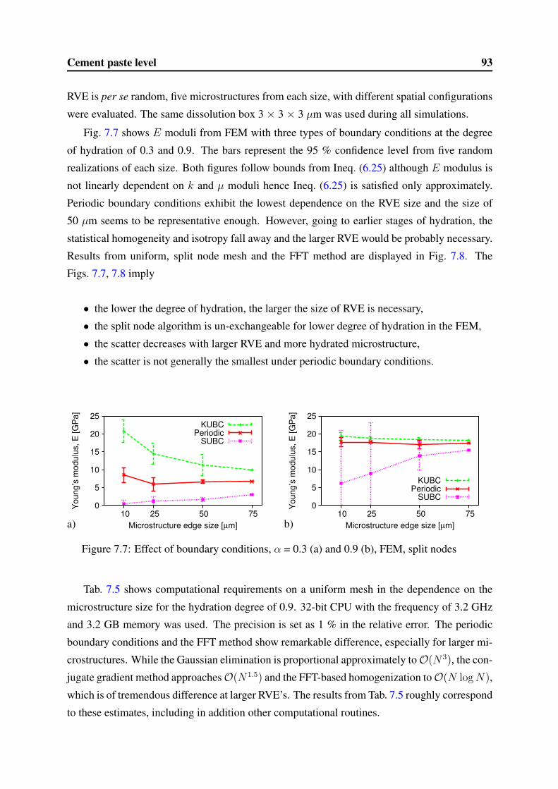
Cement paste level 93
RVE is per se random, five microstructures from each size, with different spatial configurations
were evaluated. The same dissolution box 3 × 3 × 3 µm was used during all simulations.
Fig. 7.7 shows E moduli from FEM with three types of boundary conditions at the degree
of hydration of 0.3 and 0.9. The bars represent the 95 % confidence level from five random
realizations of each size. Both figures follow bounds from Ineq. (6.25) although E modulus is
not linearly dependent on k and µ moduli hence Ineq. (6.25) is satisfied only approximately.
Periodic boundary conditions exhibit the lowest dependence on the RVE size and the size of
50 µm seems to be representative enough. However, going to earlier stages of hydration, the
statistical homogeneity and isotropy fall away and the larger RVE would be probably necessary.
Results from uniform, split node mesh and the FFT method are displayed in Fig. 7.8. The
Figs. 7.7, 7.8 imply
• the lower the degree of hydration, the larger the size of RVE is necessary,
• the split node algorithm is un-exchangeable for lower degree of hydration in the FEM,
• the scatter decreases with larger RVE and more hydrated microstructure,
• the scatter is not generally the smallest under periodic boundary conditions.
0
5
10
15
20
25
75 50 25 10
You
ng’s
mod
ulus
, E [G
Pa]
Microstructure edge size [µm]
KUBCPeriodic
SUBC
a)
0
5
10
15
20
25
75 50 25 10
You
ng’s
mod
ulus
, E [G
Pa]
Microstructure edge size [µm]
KUBCPeriodic
SUBC
b)
Figure 7.7: Effect of boundary conditions, α = 0.3 (a) and 0.9 (b), FEM, split nodes
Tab. 7.5 shows computational requirements on a uniform mesh in the dependence on the
microstructure size for the hydration degree of 0.9. 32-bit CPU with the frequency of 3.2 GHz
and 3.2 GB memory was used. The precision is set as 1 % in the relative error. The periodic
boundary conditions and the FFT method show remarkable difference, especially for larger mi-
crostructures. While the Gaussian elimination is proportional approximately toO(N3), the con-
jugate gradient method approachesO(N1.5) and the FFT-based homogenization toO(N log N),
which is of tremendous difference at larger RVE’s. The results from Tab. 7.5 roughly correspond
to these estimates, including in addition other computational routines.

Cement paste level 94
0
5
10
15
20
25
100 75 50 25 10
You
ng’s
mod
ulus
, E [G
Pa]
Microstructure edge size [µm]
Uniform meshSplit nodes
FFT
0
5
10
15
20
25
100 75 50 25 10
You
ng’s
mod
ulus
, E [G
Pa]
Microstructure edge size [µm]
Uniform meshSplit nodes
FFT
Figure 7.8: Difference among uniform, split node mesh and FFT, α = 0.3 (left) and 0.9
(right), FEM - periodic
Size [µm ] DOF’s Memory [MB] Time [s]
FEM FFT FEM FFT
10 × 10 × 10 2 997 5.7 3.1 1.6 2.6
25 × 25 × 25 46 872 71.2 6.9 24.3 6.3
50 × 50 × 50 374 997 503 35.5 218 62
75 × 75 × 75 1 265 622 1713 109 787 93
100 × 100 × 100 - - 256 - 183
Table 7.5: Approximate computational requirements on CPU 3.2 GHz, FEM - periodic, FFT
7.1.3 Paste of Kamali et al., w/c = 0.25
The dense microstructure of w/c = 0.25 was generated in the RVE size of 75 × 75 × 75
µm and hydrated with 1 µm voxel resolution, in the 3× 3× 3 µm dissolution box [57]. Tab. 7.4
again summarizes all input data for the same cement.
Fig. 7.9 shows the results for the C-S-H level as obtained via analytical Mori-Tanaka ho-
mogenization. The majority of C-S-HLD is later changed to the C-S-HHD type which causes
an increase of E modulus at this level. Self-consistent homogenization at the cement paste
level is in Fig. 7.10. The experimental data come from the same source as the previous paste
with w/c = 0.5 [57], originating in recalculation of Young’s modulus from the fitted rela-
tionship with the capillary porosity according to Eq. (7.1). The percolation threshold plays
significant role and, in this particular case, corresponds to the degree of hydration as low as
0.015. Low w/c means that high portion of cement remains unhydrated during all hardening
process, which means that the maximum degree of hydration attains approximately 0.62. The
unhydrated clinker minerals boost the stiffness of the cement paste together with the higher

Cement paste level 95
portion of C-S-HHD.
0
5
10
15
20
25
30
0 0.1 0.2 0.3 0.4 0.5 0.6 0.7
You
ng’s
mod
ulus
, E [G
Pa]
Degree of hydration [-]
C-S-HLD
C-S-HHD
Figure 7.9: Analytical results from the
C-S-H level
0 5
10 15 20 25 30 35 40 45
0 0.1 0.2 0.3 0.4 0.5 0.6 0.7
You
ng’s
mod
ulus
, E [G
Pa]
Degree of hydration [-]
FFTUnpercolated
PercolatedEmpirical formula
Figure 7.10: Analytically predicted Young’s
modulus of cement paste, compared to FFT
The percolation of solids in different RVE sizes is depicted in Fig. 7.11. The difference
is not significant and all solid phases are connected around the degree of hydration of 0.3.
Fig. 7.12 shows the evolution of Young’s modulus for the RVE sizes of 25, 50 and 75 µm under
periodic boundary conditions. Since there would be a big discrepancy between an empirical
formula, Eq. (7.1), and the results, comparison with analytical homogenization is preferred.
The FFT homogenization on the 75 × 75 × 75 µm microstructure predicts lower E modulus in
the middle region. It must be emphasized that the FFT runs on uniform mesh of the percolated
microstructure while the FEM mesh contains in addition split nodes. Early and late values
correspond well to the empirical formula and to the results from analytical homogenization.
The difference between 50 × 50 × 50 and 75 × 75 × 75 µm RVE’s is again not significant for
the whole hydration period. If unpercolated microstructures were used, the initial E modulus
of the 75 × 75 × 75 µm would start at 26.2 GPa.
0
0.2
0.4
0.6
0.8
1
0 0.05 0.1 0.15 0.2 0.25 0.3
Sol
id p
erco
latio
n [-]
Degree of hydration [-]
25 µm50 µm75 µm
Figure 7.11: Solid percolation of mi-
crostructures of different sizes
0 5
10 15 20 25 30 35 40 45
0 0.1 0.2 0.3 0.4 0.5 0.6 0.7
You
ng’s
mod
ulus
, E [G
Pa]
Degree of hydration [-]
Analytical - percol.25 µm50 µm75 µm
FFT
Figure 7.12: Effect of RVE size on E mod-
ulus, FEM - periodic, split nodes, FFT
The apparent moduli of different RVE sizes were explored again on microstructures with the
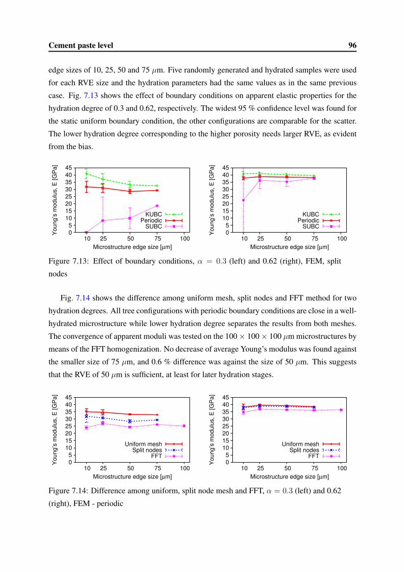
Cement paste level 96
edge sizes of 10, 25, 50 and 75 µm. Five randomly generated and hydrated samples were used
for each RVE size and the hydration parameters had the same values as in the same previous
case. Fig. 7.13 shows the effect of boundary conditions on apparent elastic properties for the
hydration degree of 0.3 and 0.62, respectively. The widest 95 % confidence level was found for
the static uniform boundary condition, the other configurations are comparable for the scatter.
The lower hydration degree corresponding to the higher porosity needs larger RVE, as evident
from the bias.
0 5
10 15 20 25 30 35 40 45
100 75 50 25 10
You
ng’s
mod
ulus
, E [G
Pa]
Microstructure edge size [µm]
KUBCPeriodic
SUBC 0 5
10 15 20 25 30 35 40 45
100 75 50 25 10
You
ng’s
mod
ulus
, E [G
Pa]
Microstructure edge size [µm]
KUBCPeriodic
SUBC
Figure 7.13: Effect of boundary conditions, α = 0.3 (left) and 0.62 (right), FEM, split
nodes
Fig. 7.14 shows the difference among uniform mesh, split nodes and FFT method for two
hydration degrees. All tree configurations with periodic boundary conditions are close in a well-
hydrated microstructure while lower hydration degree separates the results from both meshes.
The convergence of apparent moduli was tested on the 100× 100× 100 µm microstructures by
means of the FFT homogenization. No decrease of average Young’s modulus was found against
the smaller size of 75 µm, and 0.6 % difference was against the size of 50 µm. This suggests
that the RVE of 50 µm is sufficient, at least for later hydration stages.
0 5
10 15 20 25 30 35 40 45
100 75 50 25 10
You
ng’s
mod
ulus
, E [G
Pa]
Microstructure edge size [µm]
Uniform meshSplit nodes
FFT 0 5
10 15 20 25 30 35 40 45
100 75 50 25 10
You
ng’s
mod
ulus
, E [G
Pa]
Microstructure edge size [µm]
Uniform meshSplit nodes
FFT
Figure 7.14: Difference among uniform, split node mesh and FFT, α = 0.3 (left) and 0.62
(right), FEM - periodic

Cement paste level 97
7.1.4 Paste of Boumiz, w/c = 0.40
Boumiz et al. [20] measured acoustic wave velocities and the heat of hydration on white
cement paste of w/c = 0.4 and 0.35. The chemical and physical properties, as recalculated
from a mineral composition according to Bogue, are summarized in Tab. 7.6. The gypsum
content is estimated as 5 % of volume.
Component C3S C2S C3A C4AF Gypsum
Vol. content 0.7353 0.1321 0.1239 0.0087 0.05
Blaine fineness 370 m2/kg
Autocorrelation NIST files [83] danwhite
Table 7.6: Cement parameters for Boumiz’s microstructure reconstruction
The volumetric content of phases during hydration is depicted in Fig. 7.15. The voids repre-
sent an empty porosity caused by chemical shrinkage. The C-S-HHD evolves at later stages of
hydration due to the confinement as predicted with CEMHYD3D hydration model. To test the
resolution of FFT-based homogenization method, the generated set of unpercolated microstruc-
tures of 25 × 25 × 25 µm was rescaled 2, 4 and 8 times. If the homogenization is exact,
the results will be the same. Although the FFT-based method can handle an arbitrary contin-
uous field, the discontinuities in stress field cause dominantly the differences, Fig. 7.16. The
homogenized Young’s modulus is nearly the same in all four RVE’s.
0
0.2
0.4
0.6
0.8
1
0 0.1 0.2 0.3 0.4 0.5 0.6 0.7 0.8
Vol
umen
tric
fract
ion
[-]
Degree of hydration [-]
Clinker+ gypsum
CH
C-S-HLD
HDOther
WaterVoids
Figure 7.15: Volumetric content of chemical
phases during hydration
0
5
10
15
20
0 0.1 0.2 0.3 0.4 0.5 0.6 0.7 0.8
E [G
Pa]
Degree of hydration[-]
2550
100200
Figure 7.16: Homogenization of rescaled
images from 25 × 25 × 25, FFT-based ho-
mogenization
Experimental UPV data were recalculated in terms of Young’s modulus, Poisson’s ratio and
the degree of hydration from the released heat. Percolated images of the microstructure 75 ×

Cement paste level 98
75 × 75 µm were used during a FFT-based homogenization. The results for Young’s modulus,
Poisson’s ratio and experimental data are in Fig. 7.17.
0
5
10
15
20
0 0.1 0.2 0.3 0.4 0.5 0.6 0.7 0.8
You
ng’s
mod
ulus
, E [G
Pa]
Degree of hydration [-]
ExperimentFFT
0
0.1
0.2
0.3
0.4
0.5
0 0.1 0.2 0.3 0.4 0.5 0.6 0.7 0.8
Poi
sson
’s ra
tio [-
]
Degree of hydration [-]
ExperimentFFT
Figure 7.17: Results from FFT-based homogenization, percolated 75 × 75 × 75 µm,
w/c = 0.4
7.1.5 Paste of Boumiz, w/c = 0.35
A cement paste microstructure was reconstructed with the help of Tab. 7.6. Simulation
of this microstructure runs on 75 × 75 × 75 µm with 3 × 3 × 3 µm dissolution box with
the voxel resolution of 1 µm. The results from the two-level analytical homogenization are in
Figs. 7.18, 7.19 for un/percolated microstructures. The w/c of this paste corresponds roughly to
0.318 that was found to correspond for the percolation threshold of the self-consistent scheme
[17]. Fig. 7.19 shows in addition the result of the percolated microstructure when the elastic
properties of water-filled porosity are set as those of a void. It is clear that such selection
does not correspond to the experimental data. The difference in Young’s moduli from chosen
properties of the water-filled porosity is negligible (not showed).
0
5
10
15
20
25
30
0 0.1 0.2 0.3 0.4 0.5 0.6 0.7 0.8
You
ng’s
mod
ulus
, E [G
Pa]
Degree of hydration [-]
ExperimentUnpercolated
Percolated
Figure 7.18: Analytically predicted Young’s
modulus, w/c = 0.35
0
0.1
0.2
0.3
0.4
0.5
0 0.1 0.2 0.3 0.4 0.5
Poi
sson
’s ra
tio [-
]
Degree of hydration [-]
ExperimentPercolated
Unpercolated, voidPercolated, void
Figure 7.19: Analytically predicted Pois-
son’s ratio, w/c = 0.35

Cement paste level 99
One microstructure 25 × 25 × 25 µm was generated and consequently resized two and
three times. This corresponds to the voxel resolution of 1, 0.5 and 0.33 µm. In order to main-
tain the affinity between these microstructures, which was assumed, the dissolution box had to
be resized from 6 to 26 neighbors. Larger dissolution box than 3 × 3 × 3 µm is physically
unjustified since a dissolved phase might have to jump over a solid voxel [37]. FEM homog-
enization was performed on the RVE with split nodes and periodic boundary conditions. The
results from Fig. 7.20 show that the most critical parameter is the RVE size, corresponding to
a voxel resolution, and secondly the dissolving box. The smaller the dissolving box, the more
hydration is necessary for small particles in order to obtain the same hydration degree. Then the
morphology contains a large unhydrated portion of larger cement grains that are much stiffer
than the hydrated phases, which brings less homogeneous body.
0
5
10
15
20
25
30
0 0.1 0.2 0.3 0.4 0.5 0.6 0.7 0.8
You
ng’s
mod
ulus
, E [G
Pa]
Degree of hydration [-]
25 - 62x25 - 262x25 - 63x25 - 26
Experiment 0
0.1
0.2
0.3
0.4
0.5
0 0.1 0.2 0.3 0.4 0.5 0.6 0.7 0.8
Poi
sson
’s ra
tio [-
]
Degree of hydration [-]
25 - 62x25 - 262x25 - 63x25 - 26
Experiment
Figure 7.20: Effect of resolution, dissolution neighborhood and RVE size on E modulus
and Poisson’s ratio, periodic FEM with split nodes
7.1.6 BAM cement paste, w/c = 0.3
CEM I 42.5 R with the Bogue composition according to the Tab. 7.7 hydrated at 22C,
first days in the water and then under sealed conditions. The PSD is known and the amount of
particles for each diameter was taken directly from the PSD curve. The tests were conducted in
BAM (Bundesanstalt fur Materialforschung und -prufung) under Patrick Fontana.
The heat of hydration was determined in isothermal calorimeter TAM Air at 22C. There
was no superplasticizer added to the paste, therefore a suspicion was focused on particle floc-
culation. The simulation with one flocculated particle did not succeed. At later stages, the
non-evaporable water content was determined as the mass amount of water that evaporated
between 105 and 1000C.
Fig. 7.21 displays the normalized released heat, non-evaporable water content and the calori-
metric results. In addition, the released heat in 50× 50× 50 µm RVE with 6 dissolution voxels

Cement paste level 100
Component C3S C2S C3A C4AF Gypsum Anhydrite
Composition 0.492 0.243 0.090 0.076 0.025 (wt.) 0.025 (wt.)
Vol. content 0.5164 0.2496 0.100 0.0687 0.0345 0.0307
Blaine fineness 420 m2/kg
Autocorr. NIST files [83] cm115x2f
Table 7.7: Input parameters for German cement microstructure reconstruction
0
0.2
0.4
0.6
0.8
1
0.1 1 10 100 1000DoH
, oth
er v
alue
s no
rmal
ized
[-]
Time [h]
CEMHYD3D, 25x25x25Non-evaporableCalorimetry50x50x50,6
Figure 7.21: Results from simulations and
experiments
0
5
10
15
20
25
30
35
40
0 0.1 0.2 0.3 0.4 0.5 0.6 0.7 0.8
You
ng’s
mod
ulus
, E [G
Pa]
Degree of hydration [-]
FEM, periodicFFT, periodic
E before peak loadE 15% fc
Edyn
Figure 7.22: Predicted and measured elastic
properties, FEM, FFT
neighborhood is plotted, too. In this particular case, there is a better agreement with the mea-
sured data after 10 hours of hydration. The parameter β, Eq. (3.40), for cycle to time conversion
is 0.00021 for the full dissolution box and 0.00012 for 6 adjacent voxels. The calorimetric re-
sults captured the released heat during early reactions, shortly after mixing with water. On the
other hand, when only the heat after minimum heat release in the dormant period is accounted
for, the difference is about 20 J/g of cement. The potential heat was assumed as 480 J/g of
cement. Non-evaporable water content was recalculated to the degree of hydration, assuming
water consumption of 23 % by cement weight.
The percolated microstructure 25 × 25 × 25 µm was used for homogenization, Fig. 7.22.
Experimental Young’s modulus was recalculated from the stress-strain diagram of compressive
tests at various levels: shortly before the peak load and in 15 % level of the compressive strength.
As the second method, ultrasonic pulse velocities were measured. Although the data from both
methods are very similar, the discrepancy with numerical homogenization is large, especially
at early ages. The secant moduli are definitely lower then the true tangent moduli and the
results point rather to difficulties in specimen preparation and to some possible defects, e.g.
cracking. In spite of several discussions, there has not been found any reasonable explanation
of the discrepancies.

Cement paste level 101
7.1.7 Pignat’s paste, w/c = 0.45
Pignat used in the experimental program two finenesses of pure C3S cements [88]. He
measured the resonance frequency of C3S samples of w/c = 0.45, where the hydration before
testing resembled rather a sealed type of curing. The PSD for coarse and fine cements are in
Fig. 7.23.
0
0.2
0.4
0.6
0.8
1
0 10 20 30 40 50
Rel
. cum
ul. v
olum
e [-]
Grain diameter [µm]
Wcr = 0.42, C3S
measuredfit
0
0.2
0.4
0.6
0.8
1
0 10 20 30 40 50
Rel
. cum
ul. v
olum
e [-]
Grain diameter [µm]
Wcr = 0.42, C3S
measuredfit
Figure 7.23: PSD fit for coarse (left) and fine (right) cement, according to R-R distribution
Since the Pignat and Navi’s hydration model is not limited by a resolution limit, both mi-
crostructures were generated and the spherical cement grains thresholded to the smallest sphere
diameter of 0.25 µm. The surface area calculated from the spherical particles yielded directly
146 and 443 m2/kg. These values are rather underestimated since the roughness of cement
particles and their shapes are always bigger than those taken from the ideal spheres.
The best fit of points according to Rosin-Rammler distribution with van Breugel’s parame-
ters [21] yielded the Blaine fineness of 365 m2/kg for the coarse cement and 573 m2/kg for the
fine one, respectively, Fig. 7.23. The fit to the fine cement was good as opposed to the coarse
cement due to the truncation of fine particles. If the same roughness and the shape of particles
are assumed, the ratio of theoretical finenesses may be rescaled according to the fine cement fit.
This gives data of 573 m2/kg for fine and 573·146443
= 189 m2/kg for the coarse cement.
The data for elastic moduli were measured from the flexural frequencies on a simply sup-
ported cylinders with the diameter of 20 mm and the length of 130 mm for some hydration
stages [88]. The self-consistent method yields the Young’s modulus around 16 GPa for the
degree of hydration at 28 days, estimated as 0.73 by the vector model. Unfortunately, the
experimental results yielded value of only 10.8 GPa, therefore these results were not further
considered and only a numerical study was conducted.
The coarse microstructures were reconstructed in the vector and the NIST hydration model
in 100 × 100 × 100, Fig. 7.24. The volume fractions of four chemical phases were the same

Cement paste level 102
Figure 7.24: Typical microstructure slice 100 × 100 from the C3S cement paste for both
models of coarse cements, red = C3S, purple = C-S-H, blue = CH, black = water-filled
porosity, white = empty porosity. Degree of hydration is 0.7
in both models, Eq. (3.16), with the difference only in the morphology. The FFT-based ho-
mogenization had run on the digital images with the resolution of 1 µm. Moreover, the 2 µm
resolution was checked for the vector model. The homogenized Young’s moduli and Poisson’s
ratios for both unpercolated microstructures are in Fig. 7.25.
0 2 4 6 8
10 12 14 16 18
0 0.2 0.4 0.6 0.8 1
You
ng’s
mod
ulus
[GP
a]
Degree of hydration [-]
NIST 1003
Vector 503
Vector 1003
0
0.1
0.2
0.3
0.4
0.5
0 0.2 0.4 0.6 0.8 1
Poi
sson
’s ra
tio [G
Pa]
Degree of hydration [-]
NIST 1003
Vector 503
Vector 1003
Figure 7.25: Young’s modulus and Poisson’s ratio for the coarse C3S cement paste
In this particular case, the vector model with 1 µm resolution underestimates Young’s mod-
ulus values and overestimates Poisson’s ratio. This effect may be attributed only to morphology.
The same conclusion was obtained in the preliminary study of distribution, section 7.1.1.

Cement paste level 103
7.1.8 Performance of two hydration models, w/c = 0.5
Performance of Pignat and Navi’s vector hydration model and NIST discrete hydration
model was tested on coarse and fine pure C3S cement. Two microstructures in each model
with w/c = 0.5 were reconstructed, in the RVE 200 × 200 × 200 µm. The Blaine fineness was
chosen to correspond to 250 and 500 m2/kg and the PSD was obtained according to parameters
from Eqs. (3.33), (3.35), (3.36). The hydration of C3S was set up in CEMHYD3D model in
such a way that it corresponded volumetrically to Eq. (3.16) with the same densities of four
phases of Pignat and Navi’s model. The sealed conditions and isothermal curing at 20C was
prescribed. In order to maintain the volumetric content at the same hydration time, the diffusing
voxels has to be transferred to solid counterparts. The empty porosity was always transformed
to the water-filled porosity during homogenization. Fig. 7.26 shows the situation for the degree
of hydration of 0.8.
Fig. 7.27 displays the comparison of phase fractions for both models in both cements. Gen-
erally, due to digitization of a vector image, the tiny CH and C-S-H spheres yield higher vol-
umetric values than the porosity of concave-like structure. In addition, the empty porosity is
plotted for NIST hydration model.
The homogenization of FFT-based method ran on unpercolated images. The iterations were
set in such a manner that after 50 cycles the relative error had to reach up to 0.8 %. This
condition was tested in a variety of Portland cement pastes during all hydration stages against
solution after thousands of iterations and it corresponds to max. 2 % of relative error. The
vector model generally needed more iterations due to less homogeneous microstructure.
The effective bulk modulus points to a volumetrically softer microstructure from the NIST
model in the case of coarse cement. The explanation lies probably in large voids that this
hydration model creates in the places of minimal hydraulic radius. Therefore, the largest cavities
do not contain under sealed conditions any water which leads to an immobilization of hydration
products, Fig. 7.26. Also, the vector model may place portlandite around the nucleation sites
distributed randomly within the RVE. Therefore, the hydration products can be brought beyond
the C-S-H layer causing additional stiffening. If fine cement is used, no large voids appear and
the concentrical microstructure of the vector model is indeed volumetrically softer, Fig. 7.27.
On the other hand, the Young’s modulus does not reflect this change and Poisson’s ratios lay
indeed further apart. The shear moduli behave as Young’s moduli in both cements.
To conclude these comparisons, the concentrically grown microstructure is generally less
stiff than the digital one. The difference in water withdrawal mechanism and nucleation in both
models causes an exception, which is remarkable in coarse cements of higher w/c where great
areas of empty porosity are present, visible as white regions in Fig. 7.26.

Cement paste level 104
a) NIST discrete model
b) Pignat and Navi’s vector model
Figure 7.26: Coarse (left) and fine (right) microstructure of C3S paste at degree of hydra-
tion of 0.8, 200× 200 µm, w/c = 0.5, legend in Fig. 7.24
7.1.9 Leaching of cement pastes
Parametric study of cement pastes and their degraded counterparts was conducted by Kamali
et al. [57]. The study was already analyzed with a FEM code Elas3D [36]. They concluded
that the Young modulus of degraded cement paste without portlandite may reach only 50 % by

Cement paste level 105
0
0.2
0.4
0.6
0.8
1
0 0.2 0.4 0.6 0.8 1
Vol
umet
ric fr
actio
ns [-
]
Degree of hydration [-]
C3S
CH
C-S-H
Porosity
Voids
NISTVector
0
0.2
0.4
0.6
0.8
1
0 0.2 0.4 0.6 0.8 1
Vol
umet
ric fr
actio
ns [-
]
Degree of hydration [-]
C3S
CH
C-S-H
Porosity
Voids
NISTVector
0
2
4
6
8
10
12
14
16
0 0.2 0.4 0.6 0.8 1
You
ng’s
mod
ulus
[GP
a]
Degree of hydration [-]
NISTVector
0
2
4
6
8
10
12
14
16
0 0.2 0.4 0.6 0.8 1
You
ng’s
mod
ulus
[GP
a]
Degree of hydration [-]
NISTVector
0
2
4
6
8
10
12
14
0 0.2 0.4 0.6 0.8 1
Bul
k m
odul
us [G
Pa]
Degree of hydration [-]
NISTVector
0
2
4
6
8
10
12
0 0.2 0.4 0.6 0.8 1
Bul
k m
odul
us [G
Pa]
Degree of hydration [-]
NISTVector
Figure 7.27: Volumetric fractions, Young’s modulus and bulk modulus as determined for
coarse (left) and fine (right) C3S powder in discrete NIST and vector hydration model,
w/c = 0.5
the sound paste. They developed an empirical equation relating the Young modulus to capillary
porosity fraction pcap of CEMHYD3D model of sound and degraded cement pastes, Eq. (7.1).
As degradation proceeds, the portlandite, AFt, AFm, C-S-HLD and C-S-HHD become at-
tacked [48]. In this section, we limit the study only to the dissolution of portlandite. Input
cement data are the same as in section 7.1.2. It is assumed that degraded cement paste does not

Initial stress concentration 106
contain any portlandite therefore the water filled porosity is increased by its content.
The 100 × 100 × 100 well-hydrated microstructures of w/c = 0.25 and 0.5 were used with
a 3 × 3 × 3 dissolution box. The C-S-HHD prediction is again based on a confinement box of 3
× 3 × 3 voxels. Calibration to cycles was done on the basis of CH content. Degradation means
in our case the dissolution of CH in the cement paste without affecting C-S-H or AFm.
Item w/c = 0.25 w/c = 0.5
undegraded degraded undegraded degraded
Degree of hydration 0.527 0.527 0.870 0.870
Porosity (vol.) 9.7 25.4 23.2 39.6
CH (vol.) 15.7 0 16.4 0
C-S-HLD (vol.) 22.4 22.4 39.4 39.4
C-S-HHD (vol.) 18.5 18.5 12.6 12.6
E, Elas3D [GPa] 32.7 19.0 18.6 8.7
E, analytical [GPa] 32.27 19.51 15.27 6.70
E, FFT [GPa] 32.408 19.008 15.244 6.576
ν, analytical [-] 0.260 0.264 0.275 0.325
ν, FFT [-] 0.255 0.260 0.268 0.325
Table 7.8: Results from sound and leached cement pastes [57]
The results from two-level analytical homogenization combining the Mori-Tanaka and self-
consistent scheme are in a good agreement with the results from FFT-based homogenization
on percolated images, Tab. 7.8. The FEM code Elas3D predicts slightly higher values than our
FEM routine with percolation filtering and split node algorithm.
7.2 Initial stress concentration
The results for elastic calculations may point to locations where a stress may concentrate,
causing some damage at the next load increment. The failure initializes at some material point
already during an elastic behavior. Bearing this fact in mind, several material models may be
used to identify this point. The simplest 3D model without additional parameters is the Mieses-
Huber-Hencky (MHH) condition in the form of equivalent stress
σeq =√
3J2 =
√2
2
[(σx − σy)
2 + (σy − σz)2 + (σz − σx)
2 + 6(τ 2xy + τ 2
yz + τ 2zx)]1/2
, (7.2)
where J2 is the second deviatoric invariant. Although the MHH plasticity is not appropriate
for brittle materials and for materials with different compressive and tensile ultimate stress, the

Initial stress concentration 107
trends can be traced down. The well-hydrated cement with w/c = 0.5 and 0.25 were examined
using the MHH condition. The equivalent stress was calculated in all integration points across
all elements. This corresponds to a monophase porous material where all solid phases are not
distinguished. This is justified by Fagerlund’s approximation [32] that the strength is propor-
tional to a load-carrying area thus corresponding to the degree of hydration. The microstructure
10 × 10 × 10 µm was loaded by the same six components of the eigenstrain vector, with the
values of 1.0. Tab. 7.9 summarizes the results.
w/c 0.5 0.25
σmax [MPa] -214.6 -440.6
τmax [MPa] -71.5 -139.5
εmax [-] -4.41 -4.51
γmax [-] -5.4 -5.78
Internal energy [J] 61.65 126.7
Effective Young’s modulus [GPa] 19.22 39.45
σeq, max [MPa] 169.4 330.1
|σmax/σeq, max| 1.267 1.335
Table 7.9: Results of MHH analysis for w/c = 0.5 and 0.25
It is obvious that the ratio of σmax to σmax,eq is about the same for both cement pastes thus
the MHH condition makes no improvement for the strength prediction simply by some limiting
equivalent stress for all phases. In other words, the maximum stress concentration factor is
about the same in both cement pastes. Since the macroscopic stiffness ratio is around two, the
total accumulated mechanical energy by the same eigenstrain is also two times higher in these
RVE’s. If the paste with w/c = 0.5 was loaded by approximately two-times higher eigenstrain,
very similar results would come out as in the case of w/c = 0.25. Under the uniaxial loading,
the loading force is calculated as F = EAε, where E and A take into account the whole cross-
sectional area. Since A is a constant and the ultimate linear elastic stress is to be the same for
two different w/c’s, the strength is then proportional to E therefore to the degree of hydration.
This is partially supported by experiments of Igarashi et al. [53] for each sample where porosity
is directly proportional to the degree of hydration, Fig. 7.28.

Mortar level incorporating ITZ 108
Figure 7.28: Relationship between compressive strength and coarse capillary porosity, ex-
ponential and linear regressions on each w/c set [53]
7.3 Mortar level incorporating ITZ
Mortar, as a composite medium, can be considered as a three phase system: cement paste,
interfacial transition zone (ITZ) and aggregates including sand and other inert materials. Elastic
effective response of such a composite is given, as in the case of cement paste, by arrange-
ment and intrinsic properties of individual components. Considerable number of experiments
explored an effect of each phase in concrete with conclusions used further in this section. Nu-
merical and analytical modeling of concrete was done in a considerably smaller amount of
cases. As an example, a three-layer built-in analytical model [68] and numerical 2D model [81]
validated experiments on real mortar or concrete samples. Yang [131] studied the mortars using
combination of two analytical methods: firstly he homogenized a spherical aggregate together
with an ITZ by means of the double-inclusion method, and secondly using the Mori-Tanaka
theory of homogenized inclusion and bulk cement paste.
The generally accepted thickness of ITZ is 20 – 50 µm, where the cement paste compo-
sition differs significantly from the bulk one. The direct observation via an image analysis of
maturing concrete was carried out by Diamond and Huang [27] with the statement of low ce-
ment particle content in the ITZ compared to the bulk paste. They observed the wall-effect
around an aggregate but found an increase of porosity from 6 to 9 % when compared to the
mature paste. However, they attributed the reduced mechanical properties dominantly to the
wall-effect, Fig. 7.29. Since a great mechanical contrast of intrinsic properties exists between
unhydrated cement clinker and hydrated phases, the reduction of effective Young’s modulus is
quite obvious. This was supported by experiments that showed important role of this transition
zone and significant change of mechanical properties, e.g. a polymer film on the surface of
aggregates [99].
Neubauer et al. [81] found by inverse numerical simulation from the experimental values,
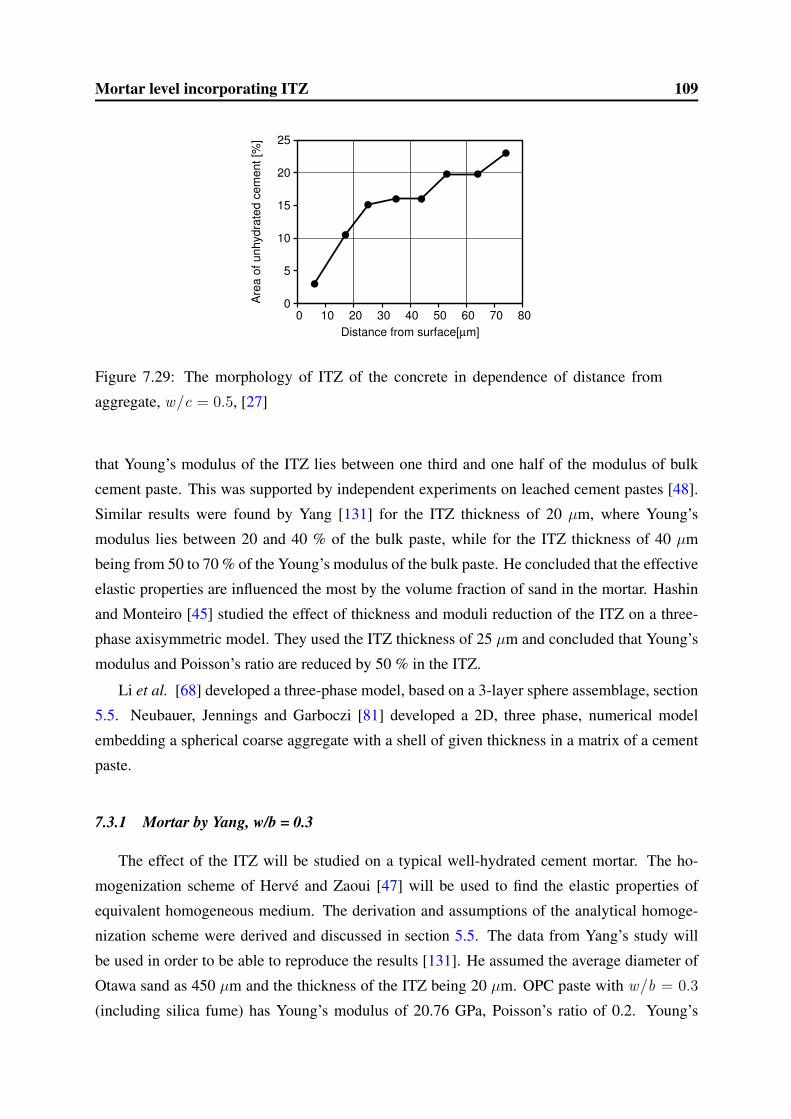
Mortar level incorporating ITZ 109
0
5
10
15
20
25
0 10 20 30 40 50 60 70 80
Are
a of
unh
ydra
ted
cem
ent [
%]
Distance from surface[µm]
Figure 7.29: The morphology of ITZ of the concrete in dependence of distance from
aggregate, w/c = 0.5, [27]
that Young’s modulus of the ITZ lies between one third and one half of the modulus of bulk
cement paste. This was supported by independent experiments on leached cement pastes [48].
Similar results were found by Yang [131] for the ITZ thickness of 20 µm, where Young’s
modulus lies between 20 and 40 % of the bulk paste, while for the ITZ thickness of 40 µm
being from 50 to 70 % of the Young’s modulus of the bulk paste. He concluded that the effective
elastic properties are influenced the most by the volume fraction of sand in the mortar. Hashin
and Monteiro [45] studied the effect of thickness and moduli reduction of the ITZ on a three-
phase axisymmetric model. They used the ITZ thickness of 25 µm and concluded that Young’s
modulus and Poisson’s ratio are reduced by 50 % in the ITZ.
Li et al. [68] developed a three-phase model, based on a 3-layer sphere assemblage, section
5.5. Neubauer, Jennings and Garboczi [81] developed a 2D, three phase, numerical model
embedding a spherical coarse aggregate with a shell of given thickness in a matrix of a cement
paste.
7.3.1 Mortar by Yang, w/b = 0.3
The effect of the ITZ will be studied on a typical well-hydrated cement mortar. The ho-
mogenization scheme of Herve and Zaoui [47] will be used to find the elastic properties of
equivalent homogeneous medium. The derivation and assumptions of the analytical homoge-
nization scheme were derived and discussed in section 5.5. The data from Yang’s study will
be used in order to be able to reproduce the results [131]. He assumed the average diameter of
Otawa sand as 450 µm and the thickness of the ITZ being 20 µm. OPC paste with w/b = 0.3
(including silica fume) has Young’s modulus of 20.76 GPa, Poisson’s ratio of 0.2. Young’s

Mortar level incorporating ITZ 110
modulus of aggregate is 80 GPa, Poisson’s ratio 0.21. He measured elastic response of that
mortar, containing volume fractions of sand as 0, 0.1, 0.2, 0.3, 0.4, and 0.5.
The first study assumes a two-phase composite: a sand grain covered with a thin layer of ITZ
of 20 µm thickness. The volume fraction of sand is 2253/2453 = 0.7745. The ITZ occupies the
rest of available space, i.e. 0.2255. Such inclusion is embedded in an equivalent homogeneous
medium. The ITZ zone will have Young’s modulus as a fraction of that of the bulk cement paste,
Poisson’s ratio will remain the same in the ITZ, i.e. ν = 0.2. Since the well-ordered moduli are
maintained for these two phases (disregarding the reference phase), the Herve-Zaoui scheme
corresponds to Hashin-Shtrikman estimation of a lower bound for a two-phase medium. The
results are in Tab. 7.10, together with Hori and Nemat-Nasser’s scheme used by Yang [131].
The lower Hashin-Shtrikman bound is significantly lower than the estimation from Hori and
Nemat-Nasser’s model.
Sand ITZ Results
EITZ/Epaste EITZ E ν k µ EHori
E = 80.000 0.0 0.000 0.000 0.200 0.000 0.000 -
ν = 0.210 0.1 2.076 13.611 0.212 7.604 5.663 35.783
k = 45.977 0.2 4.152 23.351 0.203 13.097 9.707 38.563
µ = 33.058 0.3 6.228 30.692 0.204 17.264 12.749 41.140
0.4 8.304 36.442 0.203 20.544 15.129 43.535
0.5 10.380 41.083 0.205 23.202 17.048 45.768
0.6 12.456 44.920 0.205 25.406 18.634 45.768
1.0 20.760 55.473 0.206 31.490 22.991 -
Table 7.10: Effect of ITZ properties in a cement mortar. A sand particle with 450 µm diameter
is covered with a 20 µm thick ITZ. EHori are results from Hori and Nemat-Nasser’s model [131]
In a real mortar, there are two parameters which remain unknown: the ITZ thickness and
elastic modulus in the ITZ phase (assuming the same Poisson’s ratio). Yang [130] found that
increasing the ITZ thickness is somehow equivalent to increasing the elastic modulus of the ITZ
zone. For the ITZ thickness of 20 µm, he found the results between 0.2 – 0.4 Epaste and for the
thickness of 40 µm, he deduced that Young’s modulus lies between 0.5 and 0.7 of Epaste. The
results for a 3-layered concentric spheres are in Fig. 7.30. A reasonable reduction of Young’s
modulus of the ITZ zone seems to be 0.5. The results that are in accordance with Yang [131]
and Neubauer [81].

Mortar level incorporating ITZ 111
0
5
10
15
20
25
30
35
40
0 0.1 0.2 0.3 0.4 0.5 0.6
You
ng’s
mod
ulus
[GP
a]
Volume fraction of sand [-]
EITZExperiment
0.5*Epaste0.2*Epaste
0
5
10
15
20
25
30
35
40
0 0.1 0.2 0.3 0.4 0.5 0.6
You
ng’s
mod
ulus
[GP
a]
Volume fraction of sand [-]
EITZExperiment
1.0*Epaste0.6*Epaste
Figure 7.30: Effect of ITZ thickness and Young’s modulus reduction in the ITZ on effective
properties, for ITZ thickness of 20 µm (left) and 40 µm (right)
7.3.2 Mortar B60 of Boumiz, w/c = 0.387
Boumiz et al. [20] studied the elastic properties of cement mortars with the grey OPC and
with added superplasticizer. The input parameters are in Tab. 7.11. Siliceous filler was added in
order to correct granulometric curve of sand and the plasticizer to improve workability (slightly
increased the amount of water). The more adequate name would be the concrete mortar since
grains bigger than 2 mm are used as well in the mixtures, see Tab. 7.12. The specific surface of
the cement is not known, but Bernard et al. [17] use the value of 760 m2/kg since the cement is
fast and of high performance type. The 5 vol. % content of gypsum is assumed to be added to
the cement for the setting regulation. The clinker minerals as recalculated according to Newkirk
[80], corresponding well to the input parameters as used in work of Bernard et al. [17].
Component C3S C2S C3A C4AF Gypsum
Newkirk composition 0.643 0.096 0.083 0.06 -
Vol. content 0.697 0.101 0.095 0.056 0.05
Blaine fineness 760 m2/kg
Autocorr. NIST files [83] cm115x2f
Table 7.11: Input parameters for Boumiz’s cement in B60 mortar
The simulation ran on 50 × 50 × 50 microstructure and with the 26 voxel dissolving neigh-
borhood. Fig. 7.31 shows the development of E modulus depending on previous percolation
filtering before the FFT-based homogenization. The values from the percolated microstructure
are used further. The sand is considered as E = 70 GPa, ν = 0.17, the average grain radius is

Mortar level incorporating ITZ 112
Component Size range Weight Density Volume
- [µm, mm] [kg] [g/cm3] [dm3]
Cement 0.1 – 40 µm 729.6 3.15 231.6
Water – 257.5 1.0 257.5
Sand 0 – 5 mm 1244.7 2.65 469.8
Siliceous filler 2 – 200 µm 51.5 2.65 19.4
Plasticizer (melamine-based) – 25.4 1.17 21.7
Table 7.12: Mortar composition in 1 m3, w/c = 0.387 [20]
assumed as 400 µm, the thickness of ITZ is assumed as 20 µm so the volume fraction of ITZ is
8.24 %. The coefficient of reduction of E modulus in the ITZ is 0.6 or 1.0, i.e. no reduction in
the second case. The results together with the experimental ultrasonic data are in Fig. 7.32.
0
5
10
15
20
25
0 0.2 0.4 0.6 0.8 1
You
ng’s
mod
ulus
[GP
a]
Degree of hydration [-]
UnpercolatedPercolated
Figure 7.31: Development of E modulus in
plain cement paste, FFT homogenization
0
5
10
15
20
25
30
35
40
0 0.2 0.4 0.6 0.8 1
You
ng’s
mod
ulus
[GP
a]
Degree of hydration [-]
Ered=1.0Ered=0.6
Experiment
Figure 7.32: Effect of ITZ on the homoge-
nized elastic properties of mortar
7.3.3 Mortar B35 of Boumiz, w/c = 0.524
The experiments are similar as in the previous section with slightly different cement com-
position but with the same sand [20]. The sand grain is in the range of 0 – 5 mm with an
average grain radius of 400 µm. The composition of cement and mortar is summarized in
Tabs. 7.13, 7.14.
The microstructure 50 × 50 × 50 µm ran with the 26 voxel dissolving neighborhood. The
coefficient for cycle to time scaling is 0.0003 and the dormant period was determined as 5 hours

Mortar level incorporating ITZ 113
Component C3S C2S C3A C4AF Gypsum
Newkirk composition 0.660 0.0714 0.0625 0.0626 -
Vol. content 0.720 0.077 0.094 0.058 0.05
Blaine fineness 760 m2/kg
Autocorr. NIST files [83] cm115x2f
Table 7.13: Input parameters for Boumiz’s cement in B35 mortar
Component Size range Weight Density Volume
- [µm, mm] [kg] [g/cm3 ] [dm3]
Cement 0.1 – 40 µm 567.6 3.15 180.2
Water – 292 1.0 292.1
Sand 0 – 5 mm 1335.4 2.65 503.9
Siliceous filler 2 – 200 µm 50.1 2.65 18.9
Plasticizer (melamine-based) – 5.7 1.17 4.9
Table 7.14: Mortar composition in 1 m3, w/c = 0.524 [20]
by fitting to calorimetric data, Fig. 7.33. The amount of readily soluble alkali was also fitted
to that heat curve. In addition, the affinity model with parameters from Tab. 3.2 was plotted.
Homogenized values for the cement paste together with the ITZ at the mortar level are plotted
in Fig. 7.34. Percolated cement microstructure was used, with a guaranty of nearly zero E
modulus at early ages.
0 50
100 150 200 250 300 350 400 450
0 10 20 30 40 50 0
0.1
0.2
0.3
0.4
0.5
0.6
0.7
Rel
ease
d he
at [J
/g]
Deg
ree
of h
ydra
tion
[-]
Time [h]
CEMHYD3DCalorimetry
Affinity model
Figure 7.33: Released heat during early-
ages
0
5
10
15
20
25
30
35
40
0 0.1 0.2 0.3 0.4 0.5 0.6
You
ng’s
mod
ulus
[GP
a]
Volume fraction of sand [-]
EITZExperiment
1.0*Epaste0.6*Epaste
Figure 7.34: Effect of ITZ properties on the
homogenized elastic properties of mortar

Concrete level 114
7.4 Concrete level
The results from homogenization at the cement paste or mortar level may be further upscaled
to the concrete level. Presented results are based on experiments conducted by Lee et al. [67].
A series of concrete batches was prepared and the specimens were measured in a compression
test for elastic response according to ACTM C469. The mixture proportions and cement spec-
ifications are summarized in Tab. 7.15, the unknown parameters included: amount of gypsum
in the cement, elastic properties and average radii of fine and coarse aggregates, and the ITZ
thickness.
Component C3S C2S C3A C4AF Gypsum
Blaine composition 0.54 0.1852 0.0857 0.0919 -
Vol. content 0.588 0.197 0.0987 0.086 0.03
Blaine fineness 345 m2/kg
Autocorr. NIST files [83] cm115x2f
W/c 0.5 0.27
Component Density Weight Volume Weight Volume
- [g/cm3] [kg/m3] [dm3] [kg/m3] [dm3]
Cement 3.15 370 117.4 550 174.6
Water 1.0 185 185 148 148
Plasticizer 1.0 0 0 3.55 3.55
Air - 0 30.1 0 26.5
Fine aggregates 2.51 754 300.4 617 245.8
Coarse aggregates 2.64 969 367.05 1060 401.5
Table 7.15: Cement specification and concrete composition in 1 m3, w/c = 0.5 and 0.27 [67]
For both w/c = 0.5 or 0.27, the properties were chosen in the following manner: the fine
aggregate was a siliceous sand E = 60 GPa, ν = 0.2, average diameter 1 mm and the ITZ
thickness 20 µm. The coarse aggregate was a crushed granite, E = 40 GPa, ν = 0.2, average
diameter 15 mm and the ITZ thickness 20 µm.
Since some air is present in the mixture, the first homogenization approach put the air at
the cement paste level, considered as an entrained air. The Mori-Tanaka scheme with the refer-
ence medium of cement paste was used for this purpose. The self-consistent scheme provided
very similar results since the air content was up to 3 % (vol). The multi-scale homogenization

Concrete level 115
employed further two times Herve and Zauoi’s scheme for the mortar and concrete level. The
fine aggregate at the center with an associated ITZ zone were homogenized with cement paste
including air. The reduction of Young’s modulus in the ITZ was considered as 0.5, unaffecting
the Poisson ratio. After that, the coarse aggregate at the center with an associated ITZ zone
were added to the homogenized mortar level. The elastic properties of ITZ were based again
on the cement paste. This uncoupled approach arrived to the elastic properties of concrete with
entrained air at the cement paste level.
0
5
10
15
20
25
0.5 1 2 4 8 16 32 64
You
ng’s
mod
ulus
, E [G
Pa]
Time [days]
Concrete
Mortar
Paste
8h
Paste + airExperiment
0
5
10
15
20
25
0.5 1 2 4 8 16 32 64
You
ng’s
mod
ulus
, E [G
Pa]
Time [days]
Concrete
Paste
8h
Paste + airExperiment
Figure 7.35: Young’s modulus of cement paste, mortar and concrete. Multi-scale homoge-
nization (left) and all-in-one (right), w/c = 0.5
To check the assumption of level separation, all phases above the cement paste level were
homogenized at one step (from center): coarse aggregates, associated ITZ, fine aggregates,
associated ITZ, cement paste + air. The Herve and Zaoui scheme with five spheres in a reference
medium was used again, Fig. 7.35. Although a different physical meaning of both schemes
exists, the results are not far apart. The results show a similar trend for different homogenization
levels, compare with Tab. 5.1. When the porosity from all levels, excluding intrinsic porosities
of phases, is taken to the highest level, the reduction of elastic properties is the most significant.
The set point of concrete was determined from the cement paste level and corresponds to
unrealistically high dormant period (8 and 9 hours). As long as the cement paste does not
reach the solid percolation threshold, the Herve and Zauoi scheme will predict nearly the same
low stiffness. Therefore, this homogenization scheme always guarantees that the initial period
will be treated correctly. Since no early experimental points are known, the calibration of the
CEMHYD3D hydration model was based on late experimental data only. The calibration would
not be problematic and might be used for the prediction of concrete elastic properties during the
whole hydration period.
The same experiments with the same parameters were conducted for concrete with w/c =

Concrete level 116
0.27. In this particular case, the differences in the Young modulus should be more obvious
since the cement paste has a higher stiffness. The results are again in a good agreement with
experiments, again with unrealistically long dormant period Fig. 7.36.
0
5
10
15
20
25
30
35
0.5 1 2 4 8 16 32 64
You
ng’s
mod
ulus
, E [G
Pa]
Time [days]9h
ConcreteMortarPastePaste + airExperiment
0
5
10
15
20
25
30
35
0.5 1 2 4 8 16 32 64Y
oung
’s m
odul
us, E
[GP
a]Time [days]
9h
ConcretePastePaste + airExperiment
Figure 7.36: Young’s modulus of cement paste, mortar and concrete. Mortar and concrete
level (left) and all-in-one (right), w/c = 0.27
Conclusion and future work 117
Chapter 8
CONCLUSION AND FUTURE WORK
The following research objectives were accomplished in the Ph.D. thesis:
• evolving microstructures of cement paste were predicted from initial reconstructed ce-
ment paste image. CEMHYD3D, affinity, Pignat and Navi’s hydration models were con-
sidered for this purpose and mutually compared. Implemented cement reactions were
based on the theories of Powers and his coworkers, extended with contemporary knowl-
edge of cement hydration,
• evolving microstructures were adapted for consecutive linear elastic homogenization. A
new algorithm, separating C-S-HLD and C-S-HHD at the C-S-H level was proposed and
validated for cement pastes. Proposed confinement condition is easy for implementation
and calibration, the later hydration stages agree well with the J-T model [113],
• the solid percolation filtering was introduced in order to treat early hydration ages shortly
after the solid percolation threshold. The filtering has significant effect up to the degree
of hydration of approximately 0.3,
• the microstructure of cement paste reflects an effect of chemical cement composition,
particle size distribution, hydration temperature and curing conditions in CEMHYD3D
model. The homogenization results depend upon these factors,
• analytical homogenization found perfect application at the C-S-H level, where the elastic
properties of building C-S-H units were obtained by means of inverse analysis. In addi-
tion, good results were obtained for later hydration stages of various cement pastes. The
conspherical scheme of Herve and Zauoi is indispensable for mortar and concrete level
where the appropriate morphology including ITZ is well represented. The multiscale
approach in cement-based materials can be based reasonably on analytical methods,
• numerical elastic homogenization methods provided more accurate results for the whole
hydration time at the cement paste level. The results from FEM or FFT-based approach
are mutually comparable. An introduction of split nodes in the FEM homogenization
releases a stress concentration at sharp corners without the need of RVE remeshing,

Conclusion and future work 118
• FFT-based homogenization method was found as the fastest for the RVE with periodic
boundary conditions. Good representation of stress and strain periodic fields paves the
way for precise analysis,
• FEM allows the calculation of apparent properties via static or kinematic uniform bound-
ary conditions over the RVE. The periodic boundary conditions yielded the lowest fluctu-
ation of apparent properties at various RVE sizes but not necessarily the lowest scatter,
• the need for larger RVE is remarkable especially at early ages and in higher w/c, reason-
able size is up to 50 × 50 × 50 µm in a typical cement paste.
Fig. 8.1 summarizes the Young modulus of analyzed cement pastes from this work via the
FFT-based approach. The linearity is observed when w/c ≥ 0.35, while a more progressive
growth of E modulus is observed in early hydration stages when w/c < 0.35. The reason of
such behavior is the solid percolation, significant at lower w/c’s.
0
5
10
15
20
25
30
35
40
0 0.1 0.2 0.3 0.4 0.5 0.6 0.7 0.8 0.9
You
ng’s
mod
ulus
, E [G
Pa]
Capillary porosity, pcap [-]
Kamali 0.25
BAM 0.3
46.03(1-pcap)3.16 Kamali 0.5Boumiz 0.4
Boumiz 0.35Pignat 0.45 coarse
Pignat 0.45 fine
Figure 8.1: Young’s moduli of analyzed cement pastes, FFT homogenization, RVE size
25–100 µm, empirical relation according to Eq. (7.1)
The results of FFT homogenization for the cement paste were replotted in terms of the de-
gree of hydration as well. The fit to the following formulae, covering the range w/c ∈ (0.25, 0.5)

Conclusion and future work 119
and for the whole hydration period with asymptotic properties, yields
Young′s modulus [GPa] = a(α− αp)b ≥ 0.001, (8.1)
αp = 0.0485 w/c, see Eq. (4.4), (8.2)
a =1
0.14 w/c1.35 , (8.3)
b = 2.15 w/c − 0.08, b ≤ 1. (8.4)
with the correlation coefficient of 0.989 for all disrete points in Fig. 8.2. The maximum degree
of hydration for Portland cement paste according to Hansen [41] is w/c0.36
, Fig. 8.2.
0
10
20
30
40
50
0 0.2 0.4 0.6 0.8 1
You
ng’s
mod
ulus
, E [G
Pa]
Degree of hydration [-]
Theoretical 0.2
Kamali 0.25
Fontana 0.3
Boumiz 0.35
Boumiz 0.4
Pignat 0.45 both
Kamali 0.5
MaximumDoH
Figure 8.2: Young’s moduli from the FFT homogenization, RVE size 25–100 µm, and the
fit according to Eq. (8.1)
The linear elastic homogenization model may be extended to a nonlinear material model,
e.g. creep behavior. The success of Bazant’s creep models [3] based on microprestress could
be physically justified at the C-S-H level of cement paste. The inverse analysis of experimental
data might provide intrinsic creep parameters for C-S-H and predict micromechanically the
concrete creep.

Bibliography 120
BIBLIOGRAPHY
[1] P. Acker: Micromechanical analysis of creep and shrinkage mechanisms. In: F.-J.
Ulm, Z.P. Bazant, F.H. Wittmann (Eds.), Creep, Shrinkage and Durability Mechanics
of Concrete and Other Quasi-Brittle Materials. Proc. of Sixth Int. Conference CON-
CREEP6, Elsevier, Oxford, UK, pp. 15–25, 2001.
[2] M. Avrami: Kinetics of Phase Change I. Journal of Chemical Physics, pp. 1103–1108,
1939.
[3] Z.P. Bazant, A.B. Hauggaard, S. Baweja, F.-J. Ulm: Microprestress-Solidification The-ory for Concrete Creep. I: Aging and Drying Effects. Jornal of Engineering Mechan-
ics, pp. 1188–1194, 1997.
[4] Z.P. Bazant, and S. Prasannan: Solidification theory for concrete creep: I. Formula-tion. J. Engng. Mech., 115 (8), pp. 1691–1703, 1989.
[5] J.J. Beaudoin: Comparison of mechanical properties of compacted calcium hydrox-ide and Portland cement paste systems. Cement and Concrete Research 13, pp. 319–
324, 1983.
[6] A. van Beek: Dielectric properties of young concrete, non-destructive dielectric sen-sor for monitoring the strength development of young concrete. PhD Thesis, Delft
University of Technology, Delft, 2000.
[7] F.G. Bell: A survey of the engineering properties of some anhydrite and gypsumfrom the north and midlands of England. Engineering Geology 38 (1-2), pp. 1–23,
1994.
[8] D.P. Bentz: CEMHYD3D: A Three-Dimensional Cement Hydration and Mi-crostructure Development Modeling Package. Version 2.0. Building and Fire Re-
search Laboratory Gaithersburg, Maryland 20899, 2000.
[9] D.P. Bentz: A Three-Dimensional Cement Hydration and Microstructure Program.I. Hydration Rate, Heat of Hydration, and Chemical Shrinkage. National Institute

Bibliography 121
of Standards and Technology, Building and Fire Research Laboratory, NISTIR 5756,
Gaithersburg, Maryland 20899, 1995.
[10] D.P. Bentz: CEMHYD3D: A Three-Dimensional Cement Hydration and Mi-crostructure Development Modeling Package. Version 3.0. Building and Fire Re-
search Laboratory Gaithersburg, Maryland 20899, June 2005.
[11] D.P. Bentz, E.J. Garboczi, C.J. Haecker, O.M. Jensen: Effect of cement particle sizedistribution on performance properties of Portland cement-based materials. Cement
and Concrete Research 29, pp. 1663–1671, 1999.
[12] D.P. Bentz, E.J. Garboczi, K.A. Snyder: A Hard Core/Soft shell MicrostructuralModel for Studying Percolation and Transport in Three-Dimensional CompositeMedia. Building and Fire Research Laboratory Gaithersburg, NIST, Maryland 20899,
1999.
[13] D.P. Bentz: Influence of Alkalis on Porosity Percolation in Hydrating Cement Pastes.Cement and Concrete Composites 28 (5), pp. 427-431, 2006.
[14] D.P. Bentz: Modeling the Influence of Limestone Filler on Cement Hydration UsingCEMHYD3D. Cement and Concrete Composites 28 (2), pp. 124–129, 2006.
[15] D.P. Bentz, D.A. Quenard, V. Baroghel-Bouny, E.J. Garboczi, H.M. Jennings: Mod-elling drying shrinkage of cement paste and mortar. Part I. Structural models fromnanometres to milimetres. Materials and Structures 28, pp. 450–458, 1995.
[16] R. Berliner, M. Popovici, K. W. Herwig, M. Berliner, H. M. Jennings, J. J. Thomas:
Quasielastic Neutron Scattering Study of the Effect of Water-to-Cement Ratio onthe Hydration Kinetics of Tricalcium Silicate. Cem. Concr. Res. 28 (2), pp. 231–243,
1998.
[17] O. Bernard, F.-J. Ulm, E. Lemarchand: A multiscale micromechanics-hydration modelfor the early-age elastic properties of cement-based materials. Cement and Concrete
Research 33 (9), pp. 1293–1309, 2003.
[18] J.G. Berryman: Mixture Theories for Rock Properties, in Rock Physics and Phase
Relations - A Handbook of Physical Constants, edited by T.J. Ahrens (American Geo-
physical Union, Washington DC), pp. 205–228., 1995.

Bibliography 122
[19] A. Bezjak, I. Jelenic: On the determination of rate constants for hydration processin cement pastes. Cem. Concr. Res. 10 (4), 553–563, 1980.
[20] A. Boumiz, C. Vernet, F.C. Tenoudji: Mechanical Properties of Cement Pastes andMortars at Early Ages. Advanced Cement Based Materials, pp. 94–106, 1996.
[21] K. van Breugel: Simulation of hydration and formation of structure in harden-ing cement-based materials. Second edition, Delft University Press, 1997. Parts of
it reprinted as Numerical simulation of hydration and microstructure developmentin hardening cement-based materials. Cement and Concrete Research 25 (2), pp. 319–
331 & 25 (3), pp. 522–530, 1995.
[22] S. Broadbent, J. Hammersley: Percolation processes. I. Crystals and mazes. Proc.
Camb. Phil. Soc. 53, pp. 629–641, 1957.
[23] R.M. Christensen, K.H. Lo: Solutions for effective shear properties in three phasesphere and cylinder models, J. Mech. Phys. Solids, 27, 315–330, 1979; ibid., Erratum,
J. Mech. Phys. Solids, 34, 639, 1986.
[24] G. Constantinides, F.-J. Ulm: The effect of two types of C-S-H on the elasticity ofcement-based materials: results from nanoindentation and micromechanical mod-eling. Cement and Concrete Research, 34 (1), pp. 67–80, 2004.
[25] W. Czernin: Cement Chemistry and Physics for Civil Engineers. Bauverlag GmbH,
Wiesbaden und Berlin, second edition, 1980.
[26] S. Diamond, D. Bonen: Microstructure of hardened cement paste - a new interpre-tation. J. Am. Ceram. Soc. 76 (12), pp. 2993–2999, 1993.
[27] S. Diamond, J. Huang: The ITZ in concrete - a different view based on image analysisand SEM observations. Cement and Concrete Composites 23, pp.179–188, 2001.
[28] D.D. Double, A. Hellawell, S.J. Perry: The hydration of Portland cement. Proc. R.
Soc. London A369, 1978.
[29] W. J. Drugan, J. R. Willis: A micromechanics-based nonlocal constitutive equationand estimates of representative volume element size for elastic composites. J. Mech.
Phys. Solids 44, pp. 497–524, 1996.

Bibliography 123
[30] R.J. van Eijk, H.J.H. Brouwers: Study of the relation between hydrated Portlandcement composition and leaching resistance. Cement and Concrete Research 28, pp.
815–828, 1998.
[31] J.D. Eshelby: The determination of the elastic field of an ellipsoidal inclusion andrelated problems. Proc. of Royal Society, Series A 241, pp. 376–396, 1957.
[32] G. Fagerlund: Relations between the Strength and the Degree of Hydration or Poros-ity of Cement Paste, Cement Mortar and Concrete. Cementa Report T87023, Dan-
deryd, 1987.
[33] R.F. Feldman, P.J. Sereda: A new model for hydrated Portland cement and its prac-tical implications. Engineering Journal (Canada) 53 (8/9), pp. 53–59,1970.
[34] S. Feng, B.I. Halperin, P.N. Sen: Transport properties of continuum systems near thepercolation threshold. Phys. Rev. B 35, pp. 197–214, 1987.
[35] K. Fuji, W.J. Kondo, J. Am. Ceram. Soc. 57, pp. 492–502, 1974.
[36] E.J. Garboczi: Finite Element and Finite Difference Programs for Computing theLinear Electric and Elastic Properties of Digital Images of Random Materials. NIST,
Building and Fire Research Laboratory, Gaithersburg, MD, 1998.
[37] E.J. Garboczi, D.P. Bentz: The effect of statistical fluctuation, finite size error, anddigital resolution on the phase percolation and transport properties of the NISTcement hydration model. Cem. Conc. Res. 31 (10), pp. 1501–1514, 2001.
[38] M. Geiker: Studies of Portland Cement Hydration: Measurement of ChemicalShrinkage and a Systematic Evaluation of Hydration Curves by Means of the Dis-persion Model. PhD. Thesis, Technical University of Denmark, Lyngby, 1983.
[39] N.M. Ghoniem et al. : Multiscale modelling of nanomechanics and micromechanics:an overview. Philosophical Magazine, pp. 3475–3528, 2003.
[40] A.A. Gusev: Representative volume element size for elastic composites: A numericalstudy. J. Mech. Phys. Solids, 45 (9), pp. 1449–1459, 1997.
[41] T.C. Hansen: Physical structure of hardened cement paste. A classical approach.Materiaux et Constructions 114 (19), pp. 423–436, 1986.

Bibliography 124
[42] Z. Hashin: Analysis of composite materials - a survey. ASME J. Appl. Mech. 50, pp.
481–505, 1983.
[43] Z. Hashin: The elastic moduli of heterogeneous materials. Journal of Applied Me-
chanics 29, pp. 143–150, 1962.
[44] Z. Hashin, S. Shtrikman: A variational approach to the theory of the elastic behaviorof multiphase materials. Journal of Mechanics and Physics of Solids 10, pp. 343–352,
1963.
[45] Z. Hashin, P.J.M. Monteiro: An inverse method to determine the elastic propertiesof the interphase between the aggregate and the cement paste. Cement and Concrete
Research 32, pp. 1291–1300, 2002.
[46] S. Hazanov, C. Huet: Order relationships for boundary-conditions effect in hetero-geneous bodies smaller than the representative volume. Journal of the Mechanics and
Physics of Solids 42 (12), pp. 1995–2011, 1994.
[47] E. Herve, A. Zaoui: N-layered Inclusion-based Micromechanical Modelling. Int. J.
Engng Sci. 31, pp. 1–10, 1993.
[48] F.H. Heutkamp, F.-J. Ulm: Chemomechanics of calcium leaching of cement-basedmaterials at different scales : the role of CH-dissolution and C-S-H degradation onstrength and durability performance of materials and structures. PhD thesis, De-
partment of Civil and Environmental Engineering, MIT, 2002.
[49] R. Hill: Continuum micro-mechanics of elastoplastic polycrystals. J. Mech. Phys.
Sol. 13, pp. 89–101, 1965.
[50] R. Hill: Elastic properties of reinforced solids - Some theoretical principles. Journal
of the Mechanics and Physics of Solids 11, pp. 357–372, 1963.
[51] R. Hill: Theory of mechanical properties of fiber-strengthened materials. - III: Self-consistent model. J. Mech. Phys. Solids 13, 189–198, 1965.
[52] C. Huet: Application of variational concepts to size effects in elastic heterogeneousbodies. J. Mech. Phys. Solids 38, pp. 813–841, 1990.

Bibliography 125
[53] S. Igarashi, M. Kawamura, A. Watanabe: Analysis of cement pastes and mortars bya combination of backscatter-based SEM image analysis and calculations based onthe Powers model. Cement and Concrete Composites 26, pp. 977–985, 2004.
[54] I. Jawed, J. Skalny, J.F. Young: Hydration of Portland cement. in P. Barnes: Structure
and Performance of Cements. Applied Science Publisher, 1983.
[55] H.M. Jennings: A model for the microstructure of calcium silicate hydrate in cementpaste. Cement and Concrete Research 30 (6), pp. 101–116, 2000.
[56] J.G. de Jong, H.N. Stein, J.M. Stevels: Hydration of tricalcium silicate. J. Appl. Chem.
17, 1967.
[57] S. Kamali, M. Moranville, E.G. Garboczi, S. Prene, B. Gerard: Hydrate Dissolution In-fluence on the Young’s Modulus of Cement Paste. Proc. Fracture Mechanics of Con-
crete Structures (FraMCoS-V), Li et al. (Eds.), Vail, 2004.
[58] T. Kanit et al.: Determination of the size of the representative volume element forrandom composites: statistical and numerical approach. International Journal of
Solids and Structures 40, pp. 3647–3679, 2003.
[59] H.J. Kim, C.C. Swan: Algorithms for automated meshing and and unit cell analysisof periodic composites with hierarchical tri-quadric tetrahedral elements. Interna-
tional Journal for Numerical Methods in Engineering, 2003.
[60] E.A. Koenders, K. van Breugel: Numerical modelling of autogenous shrinkage ofhardening cement paste. Cement and Concrete Research 30 (12), pp. 1911–1914, 2000.
[61] K. Kolar, T. Klecka, J. Kolısko: Vliv superplastifikatoru nove generace na objemovezmeny cementovych kompozitu. XI. mezinarodnı sympozium Sanace betonovych kon-
strukcı, kveten 2001.
[62] M. Krauss, K. Hariri, F.S. Rostasy: Non-Destructive Assessment of Mechanical Prop-erties of Concrete at Very Early Age by US Techniques - Method, Results and Mod-elling. IPACS, report BE96-3843/2001:12–5, 2001.
[63] G.T. Kuster, M.N. Toksoz: Velocity and attenuation of seismic waves in two-phasemedia: I. Theoretical formulation. Geophysics 39, pp. 587–606, 1974.

Bibliography 126
[64] D.A. Lange, H.M. Jennings, S.P. Shah: Image analysis techniques for characterizationof pore structure of cement-based materials. Cem. Concr. Res. 24 (5), pp. 841–853,
1994.
[65] J.L. Laugesen: Density functional calculations of elastic properties of portlandite,CaOH2. Cem. Concr. Res. 35 (2), pp. 199-203, 2005.
[66] F. Lea: Lea’s Chemistry of Cement and Concrete. Elsevier, fourth edition, 2004.
[67] H.K. Lee, K.M. Lee, Y.H. Kim, H. Yim, D.B. Dae: Ultrasonic in-situ monitoring ofsetting process of high-performance concrete. Cement and Concrete Research 34, pp.
631–640, 2004.
[68] G. Li, Y. Zhao, S.S. Pang: A Three-layer Built-in Analytical Modeling of Concrete.Cement and Concrete Research 28, pp. 1057–1070, 1998.
[69] F.W. Locher, W. Richartz, S. Sprung: Erstarren von Zement. Teil II: Einfluss desCalciumsulfatzusatzes. Zement-Kalk-Gips 33 (6), pp. 271–277, 1980.
[70] K. Maekawa, R. P. Chaube, T. Kishi: Modeling of Concrete Performance. E & FN
SPON (London), 1999.
[71] P.K. Mehta, P.J.M. Monteiro: Concrete - Microstructure, Properties and Materials.Prentice-Hall, Englewood Cliffs, New Jersey, 1993.
[72] J.C. Michel, H. Moulinec, P. Suquet: Effective properties of composite materials withperiodic microstructure: a computational approach. Comput. Methods Appl. Engrg.
172, pp. 109–143, 1999.
[73] S. Mindness, J.F. Young: Concrete. Prentice Hall, Inc., New Jersey, 1981.
[74] H. Moosberg-Bustnes, B. Lagerblad, E. Forssberg: The function of fillers in concrete.Mat. Struct. 37, pp. 74–81, 2004.
[75] T. Mori, K. Tanaka: Average stress in matrix and average elastic energy of materialswith misfitting inclusions. Acta Metallurgica 21 (5), pp. 1605–1609, 1973.
[76] H. Moulinec and P. Suquet: A fast numerical method for computing the linear andnonlinear mechanical properties of composites. Comptes Rendus de l’Academie des
Sciences Serie II 318 (11), pp. 1417–1423, 1994.

Bibliography 127
[77] J.C. Nadeau: A multiscale model for effective moduli of concrete incorporating ITZwater-cement ratio gradients, aggregate size distributions, and entrapped voids. Ce-
ment and Concrete Research 33, pp. 103–113, 2003.
[78] A. Nagy: Determination of E-modulus of Young Concrete With NondestructiveMethod. Journal of Materials in Civil Engineering, pp. 15–20, 1997.
[79] A.M. Neville: Properties of concrete. John Wiley & Sons, fourth edition, 1997.
[80] T. F. Newkirk: The alkali phases in Portland cement clinker. Proc. of the 3rd Int.
Symp. on the Chem. of Cem., London, pp.151–171, 1952.
[81] C.M. Neubauer, H.M. Jennings, E.J. Garboczi: A Three-Phase Model of the Elasticand Shrinkage Properties of Mortar. Advanced Cement-based Materials 4, pp. 6–20,
1996.
[82] L.F. Nielsen: Strength development in hardened cement paste: examination of someempirical equations. Materials and Structures 26, pp. 255-260, 1993.
[83] NIST, visible cement database http://visiblecement.nist.gov/
[84] I. Odler: Discussion of the paper ”A model for the microstructure of calcium silicatehydrate in cement pastes” by H. M. Jennings. Cement and Concrete Research 30, pp.
1337–1338, 2000.
[85] R.A. Olson, B.J. Christensen, R.T. Coverdale, S.J. Ford, G.M. Moss, H.M. Jennings,
T.O. Mason, E.J. Garboczi: Interpretation of the impedance spectroscopy of cementpaste via computer modelling: III. Microstructural analysis of frozen cement paste.J. Mater. Sci. 30, pp. 5078–5086, 1995.
[86] K.-B. Park, T. Noguchi, J. Plawsky: Modeling of hydration reactions using neuralnetworks to predict the average properties of cement paste. Cement and Concrete
Research 35 (9), pp. 1676-1684, 2005.
[87] C. Pignat, P. Navi, K. Scrivener: Characterization of the pore space in hardening ce-ment paste to predict the autogenous shrinkage. Laboratory of Construction materials,
Lausanne, Switzerland, 2002.

Bibliography 128
[88] C. Pignat: Simulation numerique de l’hydratation du silicate tricalcique, car-acterisation de la structure poreuse et de la permeabilite. These No. 2763, EPFL,
Lausanne, 2003.
[89] S. Popovics: Effect of Porosity on the Strength of concrete. Journal of Material 4 (2),
June, pp. 356–371, 1969.
[90] C. Porteneuve, H. Zanni, C. Vernet, K.O. Kjellsen, J.-P. Korb, D. Petit: Nuclear mag-netic resonance characterization of high- and ultrahigh-performance concrete. Ap-plication to the study of water leaching. Cem. Con. Res. 31, pp. 1887–1893, 2001.
[91] C. Porteneuve, J.-P. Korb, D. Petit, H. Zanni: Structure - texture correlation in ultra-high-performance concrete. A nuclear magnetic resonance study. Cem. Con. Res. 32,
pp. 97–101, 2002.
[92] T.C. Powers, T.L. Brownyards: Studies of physical properties of hardened Portlandcement paste. Research Laboratories of the Portland Cement Association, Chicago,
March, Bulletin 22, 1948.
[93] S.J. Preece et al.: On the initial stages of cement hydration. School of Mathematics
and Statistics, University of Birmingham, Edgbaston, B15 2TT, Kluwer Academic Pub-
lishers, 2000.
[94] A. Princigallo, K. van Breugel, G. Levita: Influence of the aggregate on the electricalconductivity of Portland cement concretes. Cement and Concrete Research 33 (11),
pp. 1755–1763, 2003.
[95] I.G. Richardson: The nature of C-S-H in hardened cements. Cement and Concrete
Research 29, pp. 1131–1147, 1999.
[96] I.G. Richardson: The nature of the hydration products in hardened cement pastes.Cement and Concrete Composites 22, pp. 97–113, 2000.
[97] M.D. Rintoul, S. Torquato: Precise determination of the critical threshold and expo-nents in a three-dimensional continuum percolation model. J. Phys. A:Math. Gen. 30,
pp. 585–592, 1997.

Bibliography 129
[98] A.P. Roberts, E.J. Garboczi: Elastic properties of model porous ceramics. J. Amer.
Ceram. Soc., 83, No. 12, pp. 3041–3048, (2000). National Institute of Standards and
Technology, Gaithersburg, MD 20899, USA, 2000.
[99] E. Sakai, J. Sugita: Composite Mechanism of Polymer Modified Cement. Cement and
Concrete Research 25, pp. 127–135, 1995.
[100] E.M. Schulson: Ice Damage to Concrete. Special report 98-6, US Army Corps of Engi-
neers, 1998.
[101] F. Schuth, K.S.W. Sing, J. Weitkamp (eds.): Handbook of Porous Solids. Chapter 6.11.
Cement as porous material, 1st edition, Wiley-vch, 2002.
[102] G. De Schutter, L. Taerwe: Degree of hydration-based description of mechanicalproperties of early age concrete. Materials and Structures, 29 (7), pp. 335–344, 1996.
[103] G. De Schutter, L. Taerwe: General hydration model for Portland cement and blastfurnace slag. Cement and Concrete Research 25 (3), pp. 593–604, 1995.
[104] K. Scrivener, P. Pratt: Back-scattered electron images of polished cement sectionsin scanning electron microscope. Proceeding of the 6th International Conference on
Cement Microscopy. New Mexico; pp.145–155, 1984.
[105] SIFEL. SImple Finite ELements. Open-source C++ package. http://cml.fsv.cvut.cz/
˜sifel/index.html
[106] P. Simeonov, S. Ahmad: Effect of transition zone on the elastic behavior of cement-based composites. Cement and Concrete Research 25, pp. 165–176, 1995.
[107] T. Slamecka, F. Skvara: The Effect of Water Ratio on Microstructure and Compo-sition of the Hydration Products of Portland Cement Pastes. Ceramics - Silikaty 46
(4), pp. 152–158, 2002.
[108] V. Smilauer, Z. Bittnar: Effects of representative cube size on the simulation of Port-land cement hydration in CEMHYD3D model. in: J. Walraven, J. Blaauwendraad, T.
Scarpas, B. Snijder (Eds.), 5th International PhD Symposium in Civil Engineering, A. A.
Balkema Publishers, pp. 581-587, 2004.

Bibliography 130
[109] Z. Sun, G. Ye, T. Voigh, S.P. Shah, K. van Breugel: Microstructural aspects of cementhydration - ultrasonic waves and numerical simulation. In: J. Walraven, J. Blaauwen-
draad, T. Scarpas, B. Snijder (Eds.), 5th International PhD Symposium in Civil Engineer-
ing, A. A. Balkema Publishers, pp. 971–979, 2004.
[110] H.F.W. Taylor: Cement Chemistry. Academic Press, New York, 1990.
[111] K. Theisen, F.L. Smidth: Quantitative determination of clinker phases and porestructure using image analysis. World Cement Resarch and Development, 1997.
[112] J.J. Thomas, H.M. Jennings, A.J. Allen: Determination of the Neutron ScatteringContrast of Hydrated Portland Cement Paste Using H2O/D2O Exchange., Advn.
Cem. Based Mat. 7, pp. 119–122, 1998.
[113] P.D. Tennis, H.M. Jennings: A model for two types of calcium silicate hydrate inthe microstructure of Portland cement pastes. Cement and Concrete Research 30, pp.
855–863, 2000.
[114] F. Tomosawa, T. Noguchi, K. Onoyama: Investigation of Fundamental MechanicalProperties of High-strength Concrete. Summaries of Technical Papers of Annual Meet-
ing of Architectural Institute of Japan, pp. 497–498, 1990.
[115] S. Torquato: Connection between the morphology and effective properties of het-erogeneous materials. Macroscopic Behavior of Heterogeneous Materials for the Mi-
crostructure 147, Am. Soc. Mech. Eng., pp. 53–65, 1992.
[116] S. Torquato: Modeling of physical properties of composite matrials. International
Journal of Solids and Structures, vol. 37, pp. 411–422, 2000.
[117] S. Torquato: Random Heterogenous Materials. Microstructure and MacroscopicProperties. Springer-Verlag, 2001.
[118] J.M. Torrenti, F. Benboudjema: Mechanical threshold of cementitious materials atearly age. Materials and Structures, vol. 38, no. 277, pp. 299–304, 2005.
[119] F. Tzschichholz, H. J. Herrmann, H. Zanni: Reaction-Diffusion Model for the Hydra-tion and Setting of Cement. Phys. Rev. E vol. 53, pp. 2629–37, 1996.

Bibliography 131
[120] L.J. Walpole: On the overall elastic moduli of composite materials. J. Mech. Phys.
Solids 17, pp. 235–251, 1969.
[121] J. Wang, J. Lubliner, P. Monteiro: Effect of ice formation on the elastic moduli ofcement paste and mortar. Cement and Concrete Research 18, pp. 874–885, 1988.
[122] F. Vallee: Modeling Drying, hydration, carbonation in thin mortars usingCEMHYD3D. Building and Fire Research Laboratory NIST, June 2000.
[123] K. Velez et al.: Determination by nanoindentation of elastic modulus and hardnessof pure constituents of Portland cement clinker. Cement and Concrete Research 31,
pp. 555–561, 2001.
[124] G.J. Verbeck, R.H. Helmuth: Structures and Physical Properties of Cement Paste.Proceedings of the 5th International Symposium on the Chemistry of Cement, V. 3, pp.
1–37, 1969.
[125] G. Washer, P. Fuchs, B. Graybeal: Elastic Properties of Reactive Powder Concrete.
International Symposium (NDT-CE 2003) of Non-Destructive Testing in Civil Engineer-
ing, 2003.
[126] M. Wierer: Multiscale Analysis of Woven Composites. PhD thesis, Czech Technical
University in Prague, CTU, 2004.
[127] E. Wirquin, M. Broda, B. Duthoit: Determination of the apparent activation energy ofone concrete by calorimetric and mechanical means. Influence of a superplasticizer.Cement and Conrete Research 32, pp. 1207–1213, 2002.
[128] F.H. Wittmann: Estimation of the modulus of elasticity of calcium hydroxide. Cement
and Concrete Research 16 (6), pp. 971–972, 1986.
[129] C.K. Yan: On homogenization and de-homogenization of composite materials. Ph.D.
Thesis. Drexel University, Philadelphia, PA, 2003.
[130] C.C. Yang, R. Huang: A Two-phase Model for Predicting the Compressive Strengthof Concrete. Cement and Concrete Research 10, vol. 26, pp. 1567–1577, 1996.
[131] C.C. Yang: Effect of the transition zone on the elastic moduli of mortar. Cement and
Concrete Research 28 (5), pp. 727–736, 1998.

Bibliography 132
[132] G. Ye, K. van Breugel, A.L.A. Fraaij: Three-dimensional microstructure analysis ofnumerically simulated cementitious materials. Cem. Concr. Res. 33, pp. 215–222,
2003.
[133] A. Zaoui: Continuum Micromechanics: Survey. Journal of Engineering Mechanics,
pp. 808–816, 2002.
[134] J. Zeman: Analysis of composite materials with random microstructure. CTU re-
ports, CVUT, Prague, 2003.

Herve-Zaoui scheme 133
Appendix A
HERVE-ZAOUI SCHEME
The problem of split spherical inclusions was solved by Herve and Zaoui [47]. The in-
teraction between adjacent phases may be reduced to stress, strain or displacement continuity,
resulting in a recurent scheme of n layers. First, consider a pure volumetric displacement in
infinity. The radial displacement field reads:
uir = Fir +
Gi
r2, (A.1)
where Fi and Gi are unknown constant. The corresponding stresses are:
σirr = 3kiFi −
4µi
r3Gi, (A.2)
σiθθ = σi
φφ = 3kiFi +2µi
r3Gi, (A.3)
σirθ = σi
rφ = σiθφ = 0. (A.4)
The interface between two spheres has the radius r = Rk. The continuity of σkrr and dis-
placement ukr is maintainted. This may be written in the compact form:
Jk(Rk)V k = Jk+1(Rk)V k+1, (A.5)
J i(Ri) =
[r 1
r2
3ki −4µi
r3
], V i =
[Fi
Gi
]. (A.6)
The reccurent scheme for the phase k + 1 is determined from the k-th phase:
N k = J−1k+1(Rk)Jk(Rk), (A.7)
V k+1 = N kV k, (A.8)
V k+1 =1∏
j=k
N jV 1 = QkV 1. (A.9)
Eq. (A.9) leads to:
F1 =1
Q11,n
Fn+1, (A.10)
and the coefficients Fk and Gk for k ∈ [1, n] are derived as:
Fk =Q11,k−1
Q11,n
Fn+1, (A.11)
Gk =Q21,k−1
Q11,n
Fn+1, (A.12)

Herve-Zaoui scheme 134
in n + 1 layer where the radius is infinite, Gn+1 = 0, thus Eq. (A.9) may be reformulated:
V n+1 = Nn
1∏j=n−1
N jV 1 = NnQn−1V 1. (A.13)
Substituing the terms for N yields the effective bulk modulus:
k =3knR
3nQ11,n−1 − rµnQ21,n−1
3R3nQ11,n−1 + 3Q21,n−1
, (A.14)
where the load of n + 1 sphere of Fn+1 may be arbitrary.
Having solved the radial displacement, the shear contributions are to be solved in the similar
manner:
uir = U i
r(r) sin2 θ cos 2φ, (A.15)
uiθ = U i
θ(r) sin θ cos θ cos 2φ, (A.16)
uiφ = U i
φ(r) sin θ cos 2φ. (A.17)
(A.18)
The unknowns parameters U ir(r), U
iθ(r), U
iφ(r) are obtained from equilibrium equations and
yield in the matrix notation:
Lk(Rk)W k = Lk+1(Rk)W k+1 , (A.19)
Li(r) =
r − 6νi
1−2νir3 3
r45−4νi
r2−2νir2
r −7−4νi
1−2νir3 − 2
r42r2
µi3νi
1−2νiµir
2 −12r5 µi
2νiµi−10µi
r3−2νir3
µi −7+2νi
1−2νiµir
2 8r5 µi
2µi+2µiνi
r3−2νir3
, W i =
Ai
Bi
Ci
Di
. (A.20)
The recurent scheme for the phase k + 1 is determined from the k-th phase:
M k = L−1k+1(Rk)Lk(Rk), (A.21)
W k+1 = M kW k, (A.22)
W k+1 =1∏
j=k
M jW 1 = P kW 1. (A.23)
Considering Bn+1 = 0, Eq. (A.23) leads to:
A1 = P22,nAn+1
P11,nP22,n − P12,nP21,n
, (A.24)
B1 = −P21,nAn+1
P11,nP22,n − P12,nP21,n
, (A.25)

Herve-Zaoui scheme 135
and the coefficients in vector W i for i ∈ [1, n + 1] are derived as:
W i =An+1
P22,nP11,n − P12,nP21,n
P i−1
P22,n
P21,n
0
0
, (A.26)
in n + 1 layer where the radius is infinite, Bn+1 = 0 and Dn+1 = 0, thus Eq. (A.23) leads to:
P41,nP22,n − P42,nP21,n = 0, (A.27)
which may be formulated as a quadratic equation that provides directly the effective shear mod-
ulus. The missing parameter is An+1 that may be selected arbitrary for the homogenization.


![ı –−•ł†ı Ÿ fl⁄ ı • ł‡ • €–Ÿ– _ ı • •fl € ‘€• flfi⁄[ÛŸ ¡] ¡ kı fl ‚ı • Œ ‘ Ÿ ‚Ÿ ¡ ‘€fi Œ ‘ł ł kı žı](https://img.pdfslide.tips/doc/110x75/612327f02eb15700be7eb6a9/-aaa-a-ia-a-a-a-aaa-a-ai-a.jpg)