linfun2

2: LINEAR FUNCTIONS AND MATRICES II

1. The rank-nullity theorem

Definition. Let V and W be vector spaces and T : V −→W a linear function.

(a) The kernel of T is subset of V :

ker(T ) = {v ∈ V |T (v) = 0W } ⊆ V.

(b) The image of W is the subset of W :

im(T ) = {w ∈W | there is an v ∈ V with T (v) = w}.

Remark. ker(T ) is a subspace of V and im(T ) is a subspace of W . Kernel andimage of a linear function are important subspaces which carry a lot of informationabout the linear function.

Theorem 3.1. Let V and W be vector spaces and T : V −→W a linear function.

(a) T is one-to-one if and only if ker(T ) = {0V }.(b) T is onto if and only if im(T ) = W .

Proof. (a) For the forward direction⇒ assume that T is a one-to-one linear functionand v ∈ ker(T ). Then T (v) = 0W = T (0V ) and v = 0V . Conversely, if ker(T ) ={0V } let u,v ∈ V with T (v) = T (u). Then, since T is linear,

0W = T (v)− T (u) = T (v − u)

and v − u ∈ ker(T ) = {0V }. Hence v − u = 0V and T is one-to-one.(b) If T is onto, then for every vector w ∈ W there is a v ∈ V with T (v) = w.Thus, im(T ) = W . Conversely, if im(T ) = W , then for every w ∈ W there is av ∈ V with T (v) = w. T is onto.

The following theorem relates the dimensions of kernel and image of a linearfunction, provided that the dimension of the vector space V is finite.

Theorem 3.2. Let V and W be vector spaces and T : V −→W a linear function.Suppose that V is finite dimensional. Then:

dim(ker(T )) + dim(im(T )) = dim(V ).

Proof. Suppose that dim(ker(T )) = r and let {v1, . . . ,vr} be a basis of ker(T ).Since every linearly independent sequence can be extended to a basis of the vectorspace, we can extend v1, . . . ,vr to a basis of V , say, {v1, . . . ,vr,vr+1, . . . ,vn} is abasis of V . The formula follows if we can show that the set {T (vr+1), . . . , T (vn)}is a basis of im(T ).

Typeset by AMS-TEX1

2 2: LINEAR FUNCTIONS AND MATRICES II

We first show that {T (vr+1), . . . , T (vn)} is a spanning set. Let w ∈ im(T ).Then there is a vector v ∈ V with T (v) = w. Since {v1, . . . ,vr,vr+1, . . . ,vn} is abasis of V , there are scalars ti ∈ R so that

v = t1v1 + . . .+ trvr + tr+1vr+1 + . . .+ tnvn.

This implies

w = T (v)

= T (t1v1 + . . .+ trvr + tr+1vr+1 + . . .+ tnvn)

= t1T (v1) + . . .+ trT (vr) + tr+1T (vr+1) + . . .+ tnT (vn)

= tr+1T (vr+1) + . . .+ tnT (vn)

The last equation follows since by assumption vi ∈ ker(T ) for all 1 ≤ i ≤ r andtherefore T (vi) = 0W for 1 ≤ i ≤ r. This shows that {T (vr+1), . . . , T (vn)} is aspanning set of im(T ).

In order to show that {T (vr+1), . . . , T (vn)} is linearly independent, suppose thatti ∈ R with

tr+1T (vr+1) + . . .+ tnT (vn) = 0W .

Since T is linear we have that

tr+1T (vr+1) + . . .+ tnT (vn) = 0W = T (tr+1vr+1 + . . .+ tnvn)

andtr+1vr+1 + . . .+ tnvn ∈ ker(T ).

Using that {v1, . . . ,vr} is a basis of ker(T ), there are scalars si ∈ R so that

tr+1vr+1 + . . .+ tnvn = s1v1 + . . .+ srvr.

Thuss1v1, . . . , srvn − tr+1vr+1 − . . .− tnvn = 0V

and si = tj = 0 for all i and j, since {v1, . . . ,vr,vr+1, . . . ,vn} is a basis of V . Thisshows that the set {T (vr+1), . . . , T (vn)} is linearly independent.

Let A be an m × n matrix and µA : Rn −→ Rm the linear function defined byµA(u) = Au for all u ∈ Rn. Let µA(ei) = Ai denote the ith column of A. Wewrite

A = [A1, . . . ,An]

where Ai ∈ Rm is the ith column of A.

Definition. (a) The column space C(A) of A is the subspace of Rm which is gener-ated by the columns of A, i.e. C(A) = span{A1, . . . ,An} ⊆ Rm.(b) The number dim(C(A)) is called the column rank of A and is denoted by Crk(A).

Remark. (a) The column space of A is the image of the linear function µA, that is,

im(µA) = span{A1, . . . ,An} = C(A).

Therefore dim(im(A)) = dim(C(A)) = Crk(A).(b) Note that the kernel of µA is the solution set of the homogeneous linear systemAx = 0.

Definition. The number dim(ker(µA)) is called the nullity of A and is denoted bynull(A).

Now Theorem 3.2 yields:

2: LINEAR FUNCTIONS AND MATRICES II 3

Theorem 3.3 (Rank-Nullity-Theorem). Let A be an m× n matrix. Then:

Crk(A) + null(A) = n.

Remark. Suppose that

A =

a1a2...

am

where ai is the ith row of A. In the previous chapter we defined the row space ofA as the subspace of Rn spanned by the rows of A:

R(A) = span{a1, . . . ,an}.

The row rank of A is the dimension of the row space of A:

Rrk(A) = dim(R(A)) = dim(span{a1, . . . ,an}).

The row rank of a matrix is easy to compute, since it does not change underelementary row operations. So, if A is an m × n matrix, we bring A into reducedechelon form D. Then the row rank of A is the number of nonzero rows of D. Sincethe row space does not change under elementary row operations, the nonzero rowsof D provide a basis of the row space R(A). Note that the column space changesunder elementary row operations and the linearly independent columns of D areNOT a bais of C(A). The following statement, however, is true:

Theorem 3.4. If A is an m× n matrix, then

Rrk(A) = Crk(A).

Proof. Suppose that D is the row reduced echelon form of A. The kernel of µA,that is, the solution set of the linear system Ax = 0, equals the solution set of thehomogeneous system Dx = 0. Thus the dimension of ker(µA) is the number of freevariables of the system Dx = 0 which is the number of columns of D without apivot one. On the other hand, the number of rows of D with pivot ones is exactlythe dimension of R(A). This gives:

Rrk(A) = n− dim(ker(A))

= n− null(A).

By Theorem 3.3:

n− null(A) = Crk(A)

and we have shown that Rrk(A) = Crk(A).

Definition. If A is an m × n matrix the rank of A, denoted rk(A), is the row (orcolumn) rank of A.


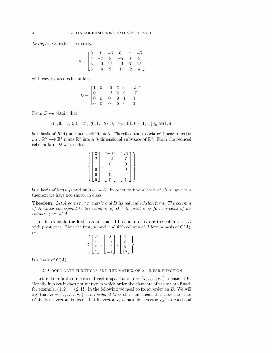
Example. Consider the matrix:

A =

0 3 −6 6 4 −53 −7 8 −5 8 93 −9 12 −9 6 153 −4 2 1 12 4

with row reduced echelon form

D =

1 0 −2 3 0 −240 1 −2 2 0 −70 0 0 0 1 40 0 0 0 0 0

.From D we obtain that

{(1, 0,−2, 3, 0,−24), (0, 1,−22, 0,−7), (0, 0, 0, 0, 1, 4)} ⊆M(1, 6)

is a basis of R(A) and hence rk(A) = 3. Therefore the associated linear functionµA : R6 −→ R4 maps R4 into a 3-dimensional subspace of R4. From the reducedechelon form D we see that

221000

,−3−20100

,

24700−41

is a basis of ker(µA) and null(A) = 3. In order to find a basis of C(A) we use atheorem we have not shown in class:

Theorem. Let A be an m×n matrix and D its reduced echelon form. The columnsof A which correspond to the columns of D with pivot ones form a basis of thecolumn space of A.

In the example the first, second, and fifth column of D are the columns of Dwith pivot ones. Thus the first, second, and fifth column of A form a basis of C(A),i.e.

0333

,

3−7−9−4

,

48612

.

is a basis of C(A).

2. Coordinate functions and the matrix of a linear function

Let V be a finite dimensional vector space and B = {v1, . . . ,vn} a basis of V .Usually in a set it does not matter in which order the elements of the set are listed,for example, {1, 2} = {2, 1}. In the following we need to fix an order on B. We willsay that B = {v1, . . . ,vn} is an ordered basis of V and mean that now the orderof the basis vectors is fixed, that is, vector v1 comes first, vector v2 is second and


so on. In particular, we consider the ordered basis B = {v1,v2, . . . ,vn} differentfrom the ordered basis B′ = {v2,v1, . . . ,vn} although the sets are the same.

We fix the order of the vectors in B and assume that B = {v1, . . . ,vn} is anordered basis of V . Then there is a unique linear function

[ ]B : V −→ Rn

defined by [ ]B(vi) = [vi]B = ei where ei is the ith standard basis vector of Rn. Ifv ∈ V with v = r1v1 + . . .+ rnvn then

[v]B = [r1v1 + . . .+ rnvn]B =

r1r2...rn

.This vector [v]B is called the coordinate vector of the vector v with respect tothe ordered basis B. The linear function [ ]B : V −→ Rn is called the coordinatefunction of V with respect to the ordered basis B.

Since [ ]B maps a basis of V onto a basis of Rn, [ ]B is an isomorphism ofvector spaces and has an inverse function LB : Rn −→ V . LB is determined byLB(ei) = vi for all 1 ≤ i ≤ n and thus is given by:

LB

t1t2...tn

= t1v1 + t2v2 + . . .+ tnvn.

Suppose now that V and W are finite dimensional vector spaces and that BV ={v1, . . . ,vn} is an ordered basis of V and BW = {w1, . . . ,wm} an ordered basis ofW . If T : V −→W is a linear function we obtain a diagram:

VT−−−−→ W

[ ]BV

y y[ ]BW

Rn Rm

The question is if we can complete this diagram in a nice way, this means, if thereis a linear function S : Rn −→ Rm so that we have a diagram

VT−−−−→ W

[ ]BV

y y[ ]BW

Rn S−−−−→ Rm

with S ◦ [ ]BV= [ ]BW

◦ T . Actually there is. Since coordinate functions areisomorphisms, there is a linear function

S = [ ]BW◦ T ◦ LB : Rn −→ Rm


with

S ◦ [ ]BV= [ ]BW

◦ T ◦ LBV◦ [ ]BV

= [ ]BW◦ T ◦ idV = [ ]BW

◦ T.

In general we define: A diagram of sets and functions

Xf−−−−→ Y

h

y ygS

`−−−−→ T

is called a commutative diagram if g ◦ f = ` ◦ h.We have just proved:

Theorem 3.5. Let V and W are vector spaces with ordered basis BV = {v1, . . . ,vn}and BW = {w1, . . . ,wm} and T : V −→W a linear function. Then there is a linearfunction S = µA : Rn −→ Rm so that the diagram

VT−−−−→ W

[ ]BV

y y[ ]BW

Rn µA−−−−→ Rm

commutes, that is, µA ◦ [ ]BV= [ ]BW

◦ T .

Definition. The m×n matrix of Theorem 3.5 is called the matrix of T with respectto ordered basis BV and BW .

Suppose as above that V and W are vector spaces with ordered basis BV ={v1, . . . ,vn} and BW = {w1, . . . ,wm} and that T : V −→ W is a linear function.We want to compute the matrix of T with respect to BV and BW . Remember thatthe function S : Rn −→ Rm is defined by:

S = [ ]BW◦ T ◦ LBV

.

Hence S = µA and the ith column of A equals S(ei) which is given by:

Ai = S(ei)

= ([ ]BW◦ T ◦ LBV

)(ei)

= ([ ]BW◦ T )(LBV

(ei)

= ([ ]BW◦ T )(vi)

= [ ]BW(T (vi))

= [T (vi)]BW.

Thus the ith column of A is [T (vi)]BWand therefore

A = [[T (v1)]BW, . . . , [T (vn)]BW

].


Example. Let T : P3 −→ P2 be the linear function defined by T (f(x)) = f ′(x). Ifwe choose for ordered basis of P3 the set B3 = {1, x, x2, x3} and for P2 the orderedbasis B2 = {1, x, x2}, then we compute

T (1) = 0 and [T (0)]B2 =

000

T (x) = 1 and [T (x)]B2

=

100

T (x2) = 2x and [T (x2)]B2

=

020

T (x3) = 3x2 and [T (x3)]B2 =

003

Thus the matrix of T with respect to basis B3 and B2 is:

A =

0 1 0 00 0 2 00 0 0 3

.If we choose different ordered basis of P3 and P2 say, B′

3 = {1, x+1, (x+1)2, (x+1)3} for P3 and B′

2 = {(x− 1)2, x− 1, 1} for P2 we have:

T (1) = 0

T (x+ 1) = 1

T ((x+ 1)2) = 2(x− 1) + 4

T ((x+ 1)3) = 3(x− 1)2 + 12(x− 1) + 12

This gives:

[T (0)]B2=

000

[T (x)]B2

=

001

[T (x2)]B2 =

024

[T (x3)]B2

=

31212

and the matrix of T with respect to the ordered basis B′

3 and B′2 is:

A′ =

0 0 0 30 0 2 120 1 4 12

.


3. Base Change

Suppose that V is a finite dimensional vector space with ordered bases B ={v1, . . . ,vn} and B′ = {u1, . . . ,un}. Let v ∈ V a vector with coordinates (withrespect to B)

[v]B =

r1r2...rn

that is, v = r1v1+ . . .+rnvn. We want to find a formula to get from the coordinatevector [v]B with respect to ordered basis B to the coordinate vector [v]B′ withrespect to B′.

The identity function idV : V −→ V is a linear function. According to section 2there is a linear function µP : Rn −→ Rn so that the following diagram commutes:

VidV−−−−→ V

[ ]B

y y[ ]B′

Rn µP−−−−→ Rn

We have that

µP ([v]B) = µP ◦ [ ]B(v)

= [ ]B′ ◦ idV (v)

= [v]B′

Thus µP maps the coordinates of a vector with respect to ordered basis B into thecoordinates of the vector with respect to ordered basis B′. This means that thereis an n× n matrix P so that

P [v]B = [v]B′ .

Definition. The n × n matrix P is called the change-of-bases-matrix from orderedbasis B to ordered basis B′.

Remark. Note that the function µP is the composition of isomorphisms:

µP = [ ]B′ ◦ idV ◦ LB = [ ]B′ ◦ LB .

In particular, µP is an isomorphism and P is an invertible matrix.

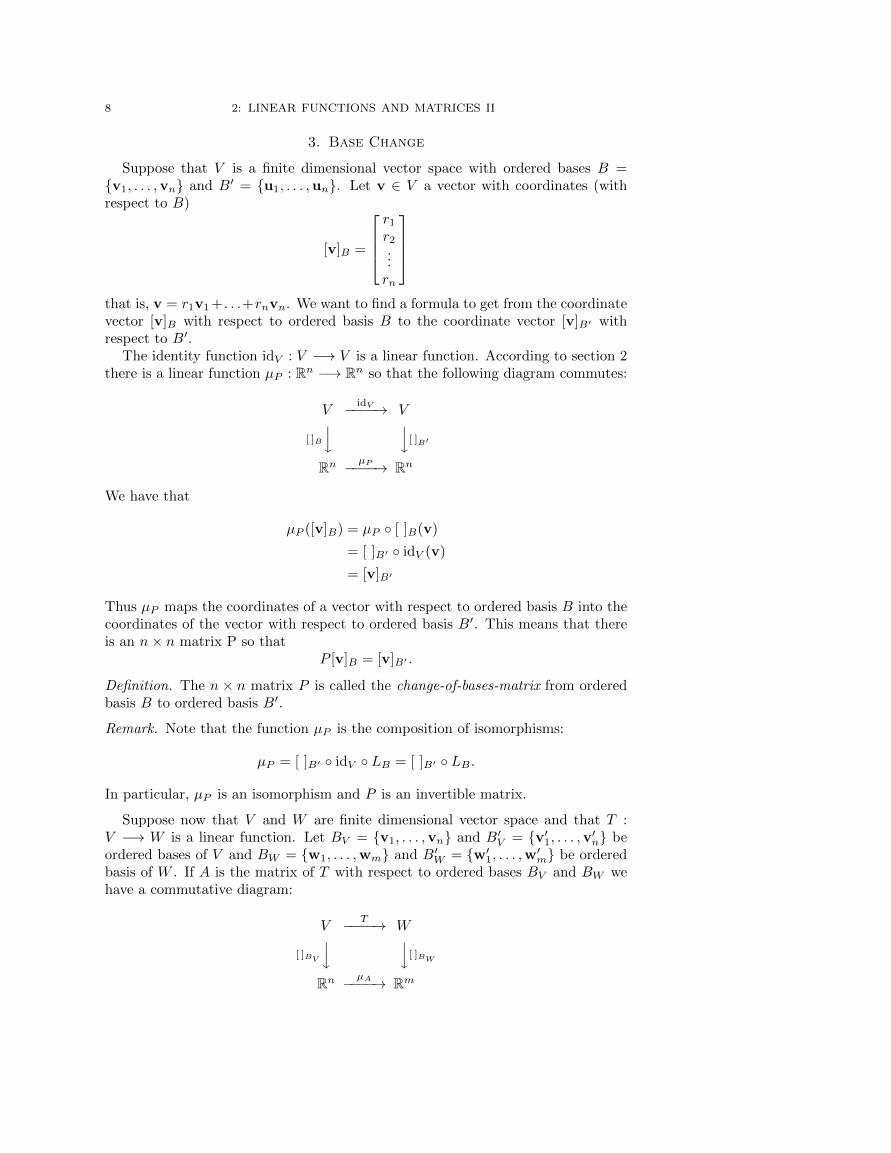
Suppose now that V and W are finite dimensional vector space and that T :V −→ W is a linear function. Let BV = {v1, . . . ,vn} and B′

V = {v′1, . . . ,v

′n} be

ordered bases of V and BW = {w1, . . . ,wm} and B′W = {w′

1, . . . ,w′m} be ordered

basis of W . If A is the matrix of T with respect to ordered bases BV and BW wehave a commutative diagram:

VT−−−−→ W

[ ]BV

y y[ ]BW

Rn µA−−−−→ Rm


We want to compute the matrix B of T with respect to the bases B′V and B′

W . LetP denote the change-of-bases-matrix for changing from basis B′

V to basis BV , Thisgives a commutative diagram:


[ ]B′V

y y[ ]BV

Rn µP−−−−→ Rn

If Q is the change-of-bases-matrix from basis BW to basis B′W we obtain a third

commutative diagram:

WidW−−−−→ W

[ ]BW

y y[ ]B′W

RmµQ−−−−→ Rm

Using these three commutative diagrams we obtain a big diagram:


T−−−−→ WidW−−−−→ W

[ ]B′V

y [ ]BV

y [ ]BW

y y[ ]B′W

Rn µP−−−−→ Rn µA−−−−→ RmµQ−−−−→ Rm

All squares in this diagram commute again. Thus the big (exterior diagram) givesa commutative diagram:

VT−−−−→ W

[ ]B′V

y y[ ]BW

RnµQAP−−−−→ Rm

where µQAP = µQ ◦ µA ◦ µP . We have just shown:

Theorem 3.6. Let T : V −→ W be a linear function of finite dimensional vectorspaces. If A is the matrix of T with respect to ordered bases BV and BW , then thematrix of T with respect to ordered bases B′

V and B′W is

QAP

where P is the change-of-bases-matrix from B′V to BV and Q is the change-of-

bases-matrix from BW to B′W .

Example. In the previous section we studied the differentiation function T : P3 −→P2. We found that the matrix of T with respect to ordered bases B3 = {1, x, x2, x3}and B2 = {1, x, x2} is:

A =

0 1 0 00 0 2 00 0 0 3

.With respect to the ordered bases B′

3 = {1, x + 1, (x + 1)2, (x + 1)3} and B′2 =

{(x− 1)2, x− 1, 1} the matrix of T is:

A′ =

0 0 0 30 0 2 120 1 4 12

.


Since

1 = 1

x+ 1 = x+ 1

(x+ 1)2 = x2 + 2x+ 1

(x+ 1)3 = x3 + 3x2 + 3x+ 1

the change-of-bases-matrix from B′3 to B3 is:

P =

1 1 1 10 1 2 30 0 1 30 0 0 1

.Similarly,

1 = 1

x = (x− 1) + 1

x2 = (x− 1)2 + 2(x− 1) + 1

and

Q =

0 0 10 1 21 1 1

is the change-of-bases-matrix from ordered basis B2 to ordered basis B′

2. Then

QAP =

0 0 10 1 21 1 1

0 1 0 00 0 2 00 0 0 3

1 1 1 10 1 2 30 0 1 30 0 0 1

=

0 0 10 1 21 1 1

0 1 2 30 0 2 60 0 0 3

=

0 0 0 30 0 2 120 1 4 12

= A′.

Documents

linfun2