Long range tracking radar system

23rd Sino-Japanese Engineering Technology Seminar

CSIST Part

October 28th 2003

Tatsukichi Koshio 小塩 立吉

Guest Researcher, Takushoku University 拓殖大学客員研究員 Technical Advisor, Tokyo Keiso Co., Ltd. 東京計装株式会社 技術顧問

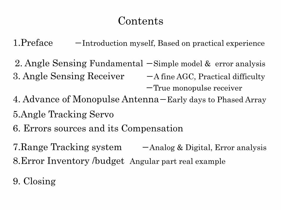
Contents

1.Preface －Introduction myself, Based on practical experience 2. Angle Sensing Fundamental －Simple model & error analysis 3. Angle Sensing Receiver －A fine AGC, Practical difficulty －True monopulse receiver 4. Advance of Monopulse Antenna－Early days to Phased Array

5.Angle Tracking Servo 6. Errors sources and its Compensation 7.Range Tracking system －Analog & Digital, Error analysis 8.Error Inventory /budget Angular part real example 9. Closing

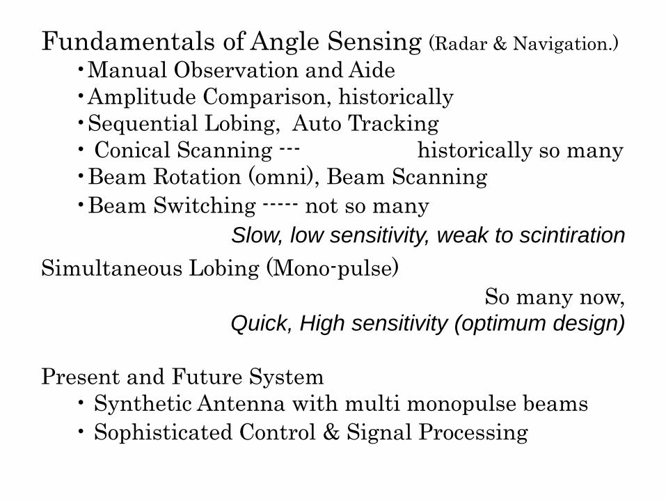
Fundamentals of Angle Sensing (Radar & Navigation.) •Manual Observation and Aide •Amplitude Comparison, historically •Sequential Lobing, Auto Tracking • Conical Scanning --- historically so many •Beam Rotation (omni), Beam Scanning •Beam Switching ----- not so many

Slow, low sensitivity, weak to scintiration Simultaneous Lobing (Mono-pulse)

So many now, Quick, High sensitivity (optimum design)

Present and Future System

• Synthetic Antenna with multi monopulse beams • Sophisticated Control & Signal Processing

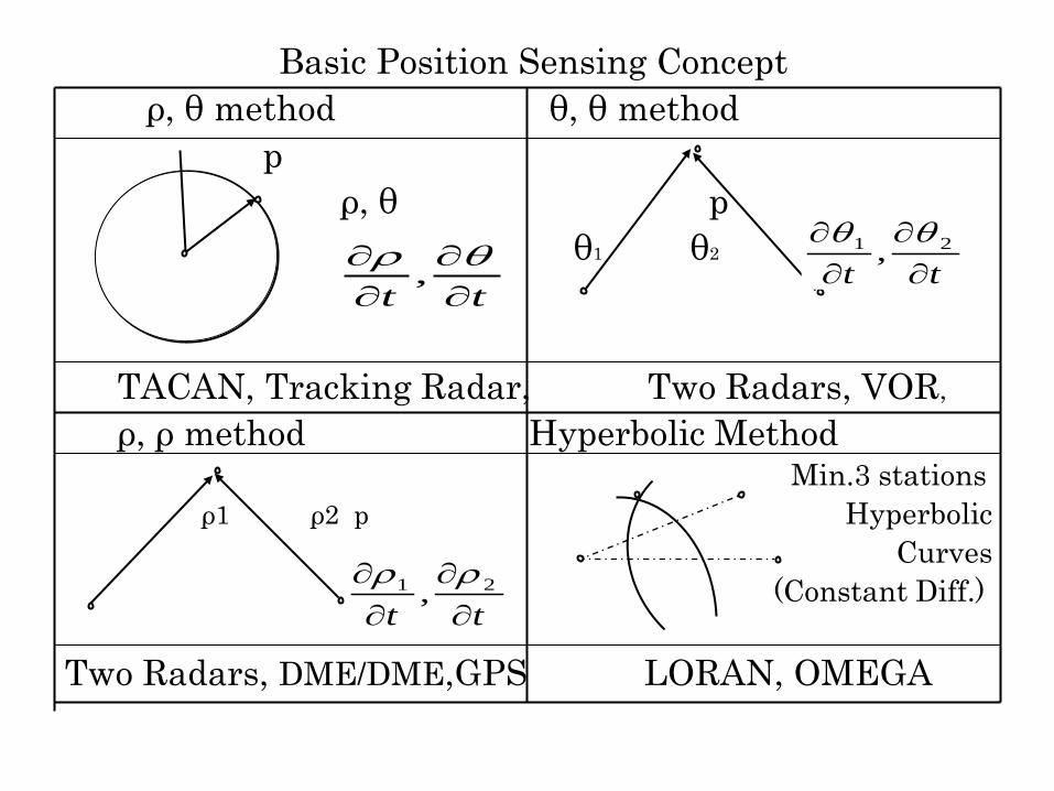
Basic Position Sensing Concept ρ, θ method θ, θ method p ρ, θ p θ1 θ2 TACAN, Tracking Radar, Two Radars, VOR, ρ, ρ method Hyperbolic Method Min.3 stations

ρ1 ρ2 p Hyperbolic Curves

(Constant Diff.)

Two Radars, DME/DME,GPS LORAN, OMEGA tt ∂

∂∂∂ 21 , ρρ

tt ∂∂

∂∂ θρ , tt ∂

∂∂∂ 21 , θθ

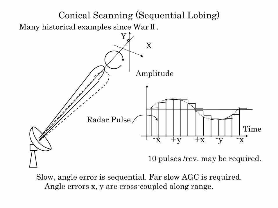
Conical Scanning (Sequential Lobing) Many historical examples since WarⅡ. Y X Amplitude Radar Pulse

Time -x +y +x -y -x

10 pulses /rev. may be required.

Slow, angle error is sequential. Far slow AGC is required. Angle errors x, y are cross-coupled along range.

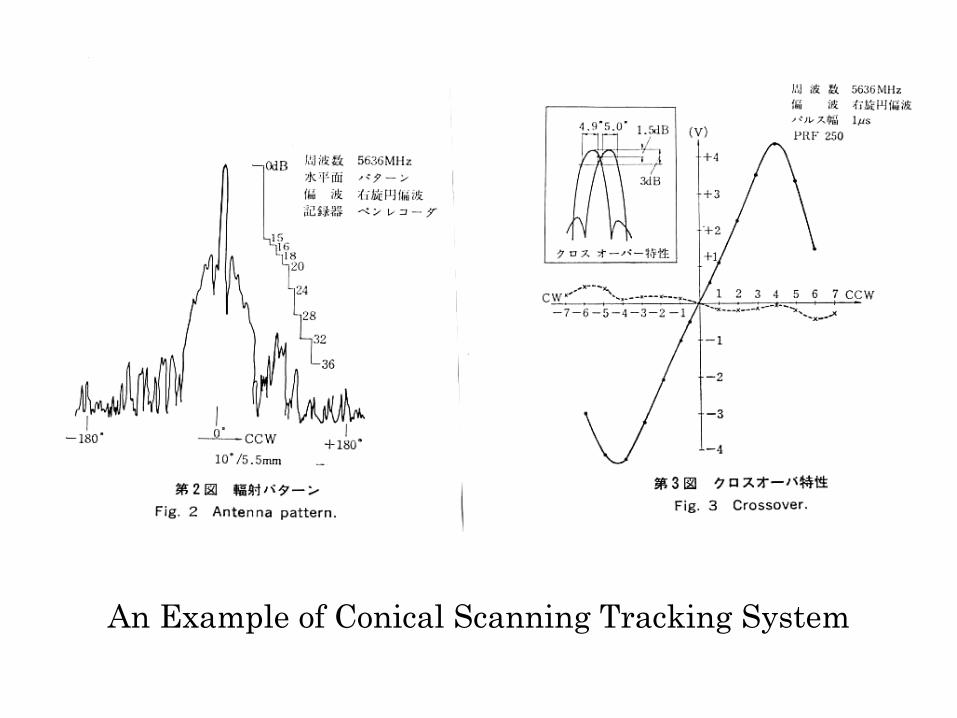
An Example of Conical Scanning Tracking System

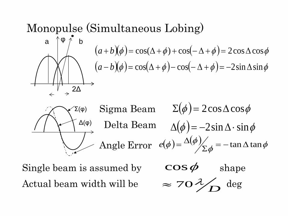
Monopulse (Simultaneous Lobing)

( ) φφ coscos2 ∆=Σ

( ) ( ) φφφφ tantan∆−=Σ

∆=e

φcos

Dλ70≈

Sigma Beam

Delta Beam

Angle Error

Single beam is assumed by Actual beam width will be

a b φ

2Δ

shape deg

Σ(φ)

Δ(φ)

( )( ) ( ) ( ) φφφφ sinsin2coscos ∆−=+∆−−+∆=− ba

( )( ) ( ) φφφφ coscos2cos)cos( ∆=+∆−++∆=+ ba

( ) φφ sinsin2 ⋅∆−=∆

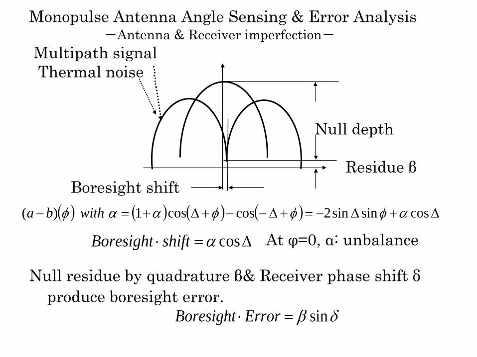
Monopulse Antenna Angle Sensing & Error Analysis －Antenna & Receiver imperfection－ Multipath signal Thermal noise Null depth Residue β

Null residue by quadrature β& Receiver phase shift δ produce boresight error.

( ) ( ) ( ) ( ) ∆+∆−=+∆−−+∆+=− cossinsin2coscos1)( αφφφααφ withba

∆=⋅ cosαshiftBoresight

δβ sin=⋅ErrorBoresight

At φ=0, α: unbalance

Boresight shift

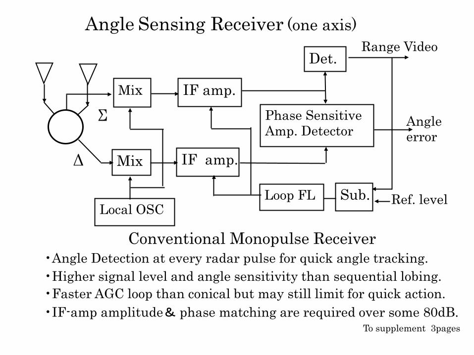
Mix

Mix

Local OSC

IF amp.

IF amp.

Phase Sensitive Amp. Detector

Sub. Loop FL

Det.

Angle Sensing Receiver (one axis)

Conventional Monopulse Receiver •Angle Detection at every radar pulse for quick angle tracking. •Higher signal level and angle sensitivity than sequential lobing. •Faster AGC loop than conical but may still limit for quick action. •IF-amp amplitude＆ phase matching are required over some 80dB.

To supplement 3pages

Range Video

Angle error

Ref. level

Δ

Σ

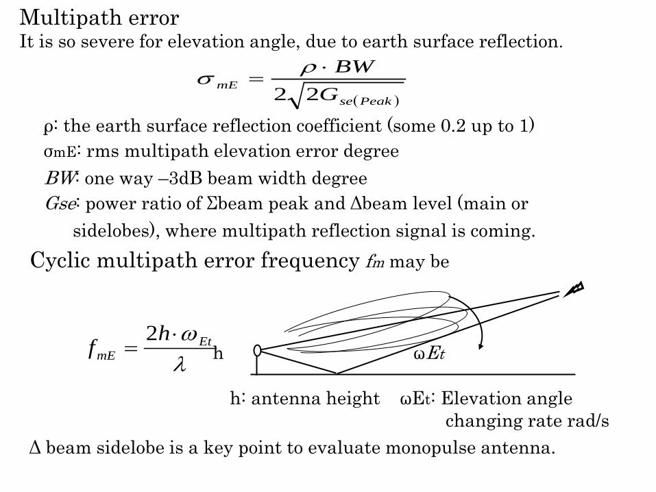
Multipath error It is so severe for elevation angle, due to earth surface reflection. ρ: the earth surface reflection coefficient (some 0.2 up to 1) σmE: rms multipath elevation error degree BW: one way –3dB beam width degree Gse: power ratio of Σbeam peak and Δbeam level (main or sidelobes), where multipath reflection signal is coming. Cyclic multipath error frequency fm may be h ωEt h: antenna height ωEt: Elevation angle changing rate rad/s Δ beam sidelobe is a key point to evaluate monopulse antenna.

( )PeaksemE G

BW22⋅

=ρσ

λωEt

mEhf ⋅

=2

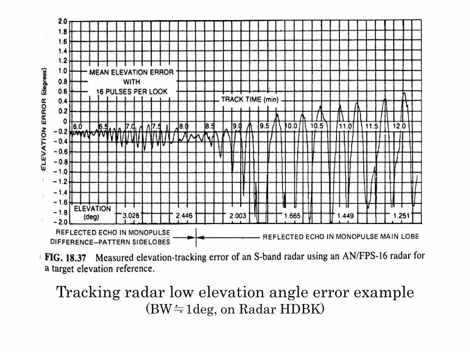
Tracking radar low elevation angle error example (BW≒1deg, on Radar HDBK)

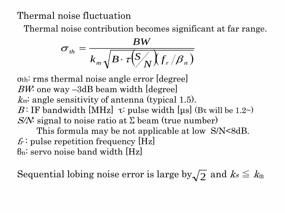
Thermal noise fluctuation Thermal noise contribution becomes significant at far range. σth: rms thermal noise angle error [degree] BW: one way –3dB beam width [degree] km: angle sensitivity of antenna (typical 1.5). B : IF bandwidth [MHz] τ: pulse width [μs] (Bτ will be 1.2~) S/N: signal to noise ratio at Σ beam (true number) This formula may be not applicable at low S/N<8dB. fr : pulse repetition frequency [Hz] βn: servo noise band width [Hz] Sequential lobing noise error is large by and ks ≦ km

( )( )nrm

thfN

SBk

BW

βτσ

⋅=

2

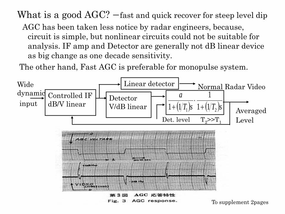
What is a good AGC? －fast and quick recover for steep level dip AGC has been taken less notice by radar engineers, because,

circuit is simple, but nonlinear circuits could not be suitable for analysis. IF amp and Detector are generally not dB linear device as big change as one decade sensitivity.

The other hand, Fast AGC is preferable for monopulse system.

Controlled IF dB/V linear

Detector V/dB linear

Linear detector Wide dynamic input

Normal Radar Video

Det. level T2>>T1 Averaged Level

To supplement 2pages

( ) ( )sTsTa

21 111

11 +⋅

+

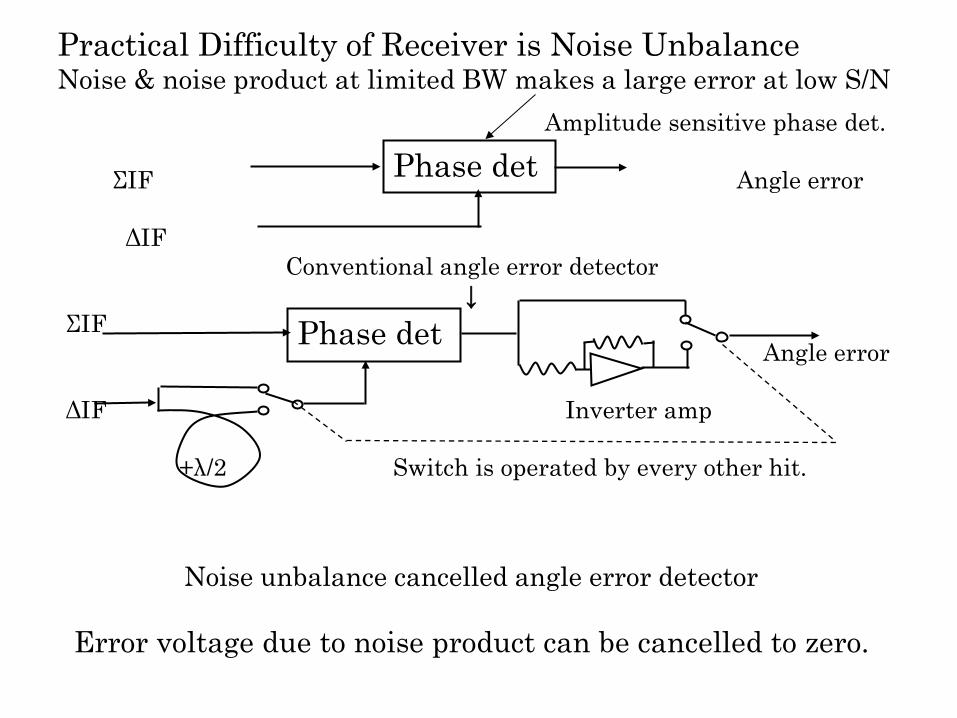
Practical Difficulty of Receiver is Noise Unbalance Noise & noise product at limited BW makes a large error at low S/N

Phase det

Phase det

Amplitude sensitive phase det. ΣIF Angle error ΔIF Conventional angle error detector ↓ ΣIF Angle error ΔIF Inverter amp +λ/2 Switch is operated by every other hit.

Noise unbalance cancelled angle error detector Error voltage due to noise product can be cancelled to zero.

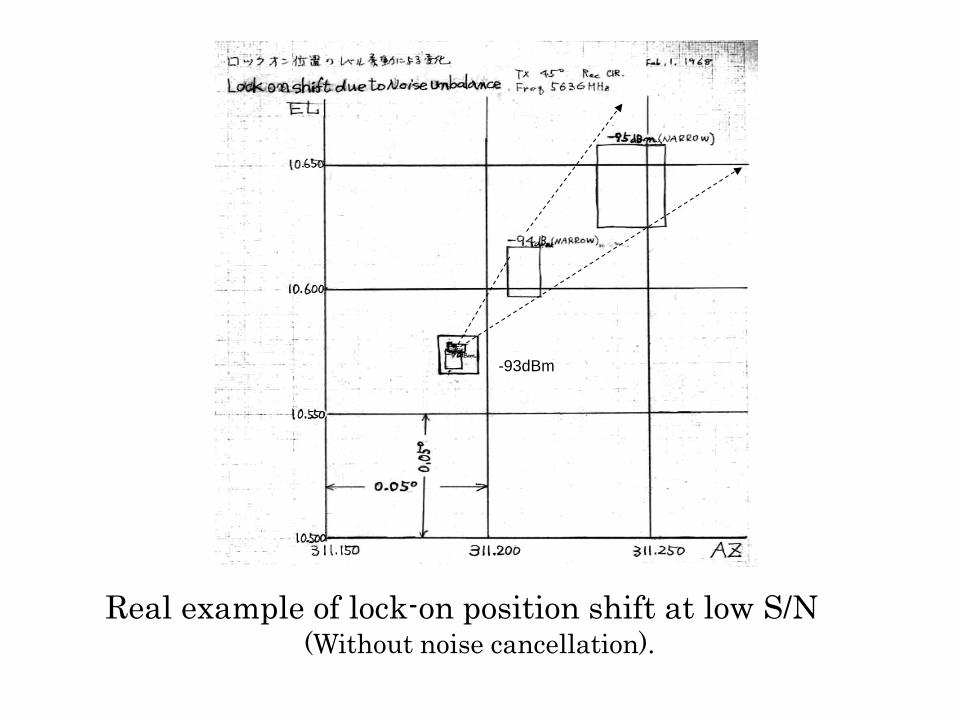
Real example of lock-on position shift at low S/N

(Without noise cancellation).

-93dBm

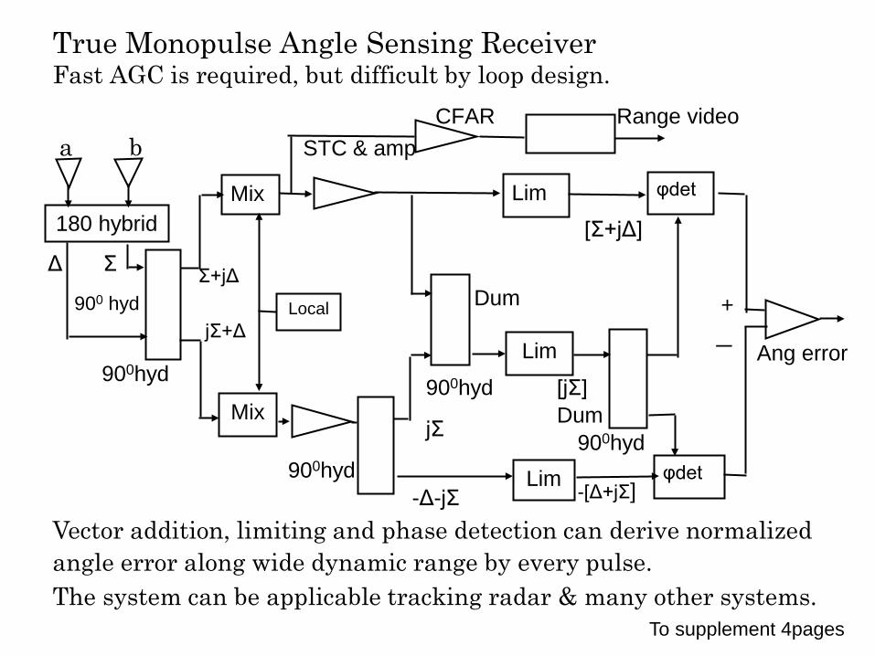
True Monopulse Angle Sensing Receiver Fast AGC is required, but difficult by loop design. CFAR Range video a b STC & amp 180 hybrid

Mix Lim φdet

Mix

Local

Lim

Lim φdet

Vector addition, limiting and phase detection can derive normalized angle error along wide dynamic range by every pulse. The system can be applicable tracking radar & many other systems.

Δ Σ Σ+jΔ

jΣ+Δ 900 hyd

[Σ+jΔ]

Dum

jΣ

900hyd 900hyd

-Δ-jΣ

[jΣ]

900hyd -[Δ+jΣ]

+

－ Ang error

900hyd Dum

To supplement 4pages

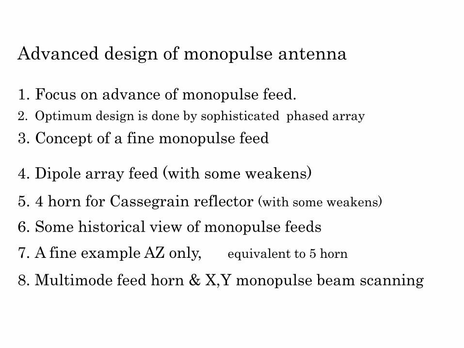
Advanced design of monopulse antenna 1. Focus on advance of monopulse feed. 2. Optimum design is done by sophisticated phased array 3. Concept of a fine monopulse feed

4. Dipole array feed (with some weakens) 5. 4 horn for Cassegrain reflector (with some weakens)

6. Some historical view of monopulse feeds 7. A fine example AZ only, equivalent to 5 horn

8. Multimode feed horn & X,Y monopulse beam scanning

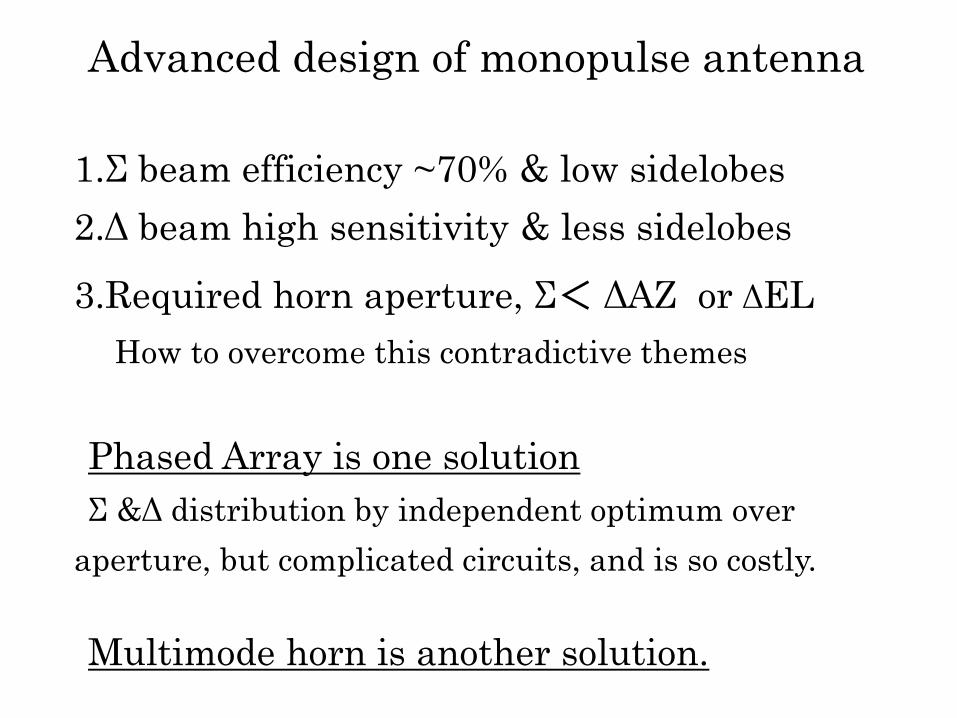
Advanced design of monopulse antenna

1.Σ beam efficiency ~70% & low sidelobes 2.Δ beam high sensitivity & less sidelobes

3.Required horn aperture, Σ＜ ΔAZ or ΔEL How to overcome this contradictive themes Phased Array is one solution Σ &Δ distribution by independent optimum over

aperture, but complicated circuits, and is so costly. Multimode horn is another solution.

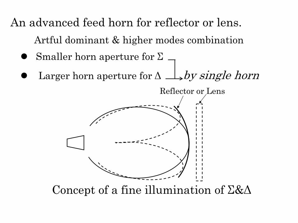
An advanced feed horn for reflector or lens. Artful dominant & higher modes combination

Smaller horn aperture for Σ

Larger horn aperture for Δ by single horn Reflector or Lens

Concept of a fine illumination of Σ&Δ

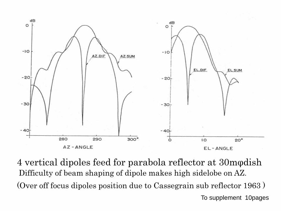
4 vertical dipoles feed for parabola reflector at 30mφdish Difficulty of beam shaping of dipole makes high sidelobe on AZ. (Over off focus dipoles position due to Cassegrain sub reflector 1963 )

To supplement 10pages

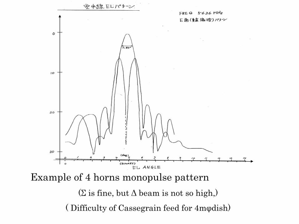
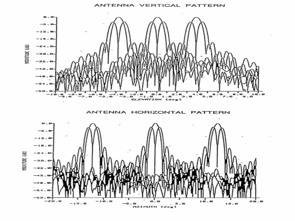
Example of 4 horns monopulse pattern (Σ is fine, but Δ beam is not so high,)

( Difficulty of Cassegrain feed for 4mφdish)

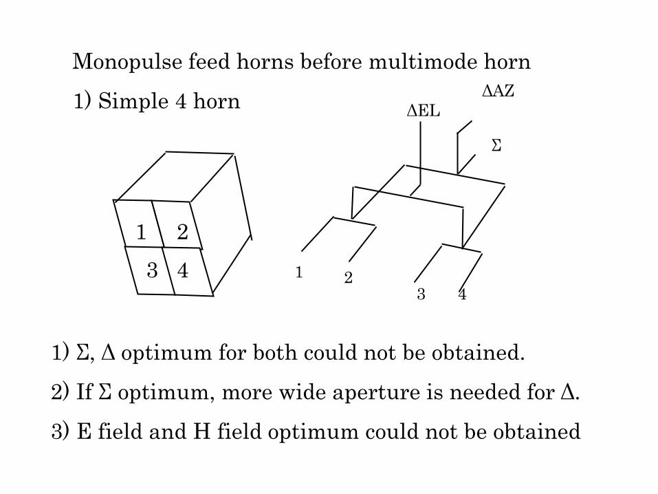
Monopulse feed horns before multimode horn 1) Simple 4 horn

ΔAZ ΔEL

Σ

1

2 3 4

1) Σ, Δ optimum for both could not be obtained. 2) If Σ optimum, more wide aperture is needed for Δ. 3) E field and H field optimum could not be obtained

1 2 3 4

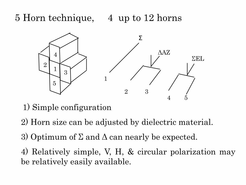
5 Horn technique, 4 up to 12 horns

1) Simple configuration 2) Horn size can be adjusted by dielectric material. 3) Optimum of Σ and Δ can nearly be expected. 4) Relatively simple, V, H, & circular polarization may be relatively easily available.

1 2 3

4

5 1

Σ

2 3

ΔAZ ΣEL

4 5

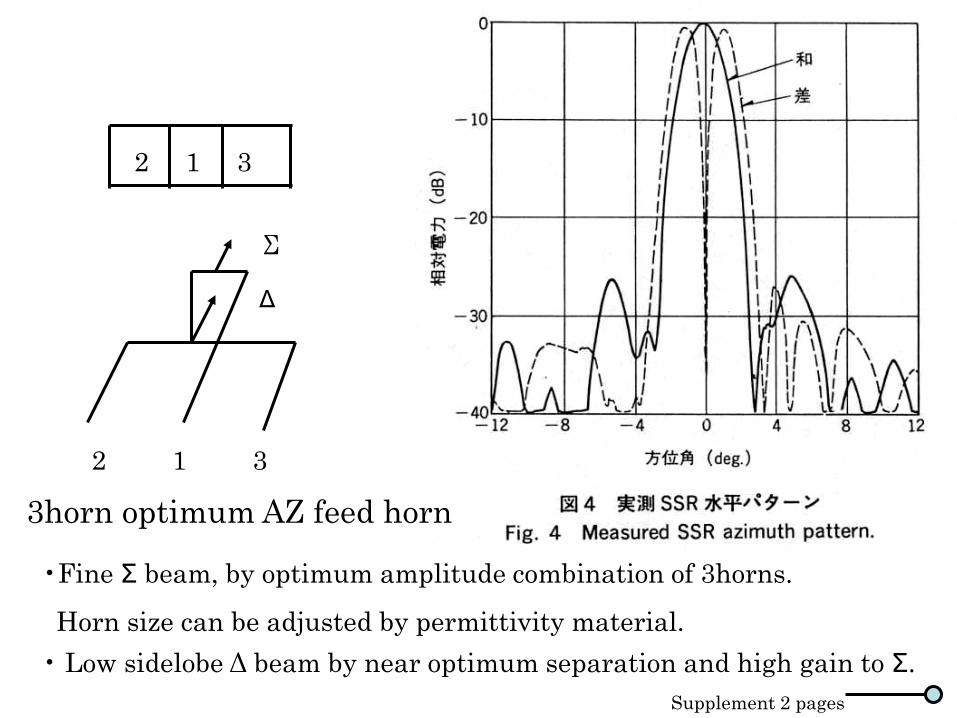
2 1 3

2 1 3

Σ

Δ

•Fine Σ beam, by optimum amplitude combination of 3horns.

Horn size can be adjusted by permittivity material. • Low sidelobe Δ beam by near optimum separation and high gain to Σ.

3horn optimum AZ feed horn

Supplement 2 pages

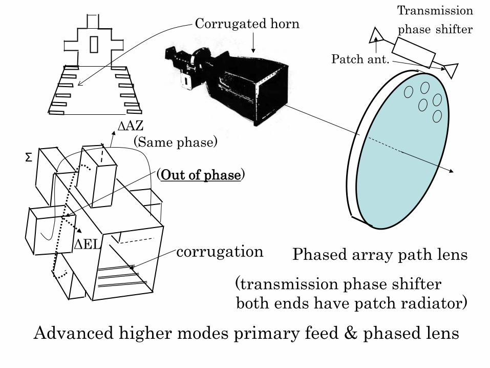
Σ

ΔAZ (Same phase)

Corrugated horn

ΔEL

(Out of phase)

Phased array path lens (transmission phase shifter both ends have patch radiator)

corrugation

Patch ant.

Transmission phase shifter

Advanced higher modes primary feed & phased lens

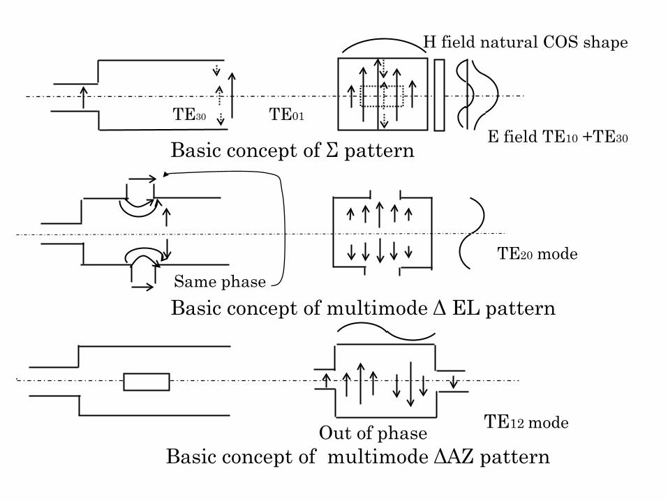
Basic concept of multimode Δ EL pattern

H field natural COS shape

Basic concept of Σ pattern E field TE10 +TE30

TE01 TE30

Same phase TE20 mode

Basic concept of multimode ΔAZ pattern TE12 mode Out of phase

＋ ＝

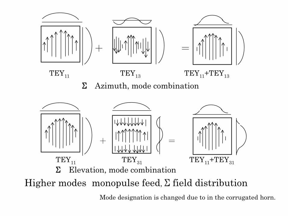
TEY11 TEY13 TEY11+TEY13

Σ Azimuth, mode combination

TEY11 TEY31 TEY11+TEY31 Σ Elevation, mode combination

＋ ＝

Higher modes monopulse feed, Σ field distribution Mode designation is changed due to in the corrugated horn.

＋ ＝

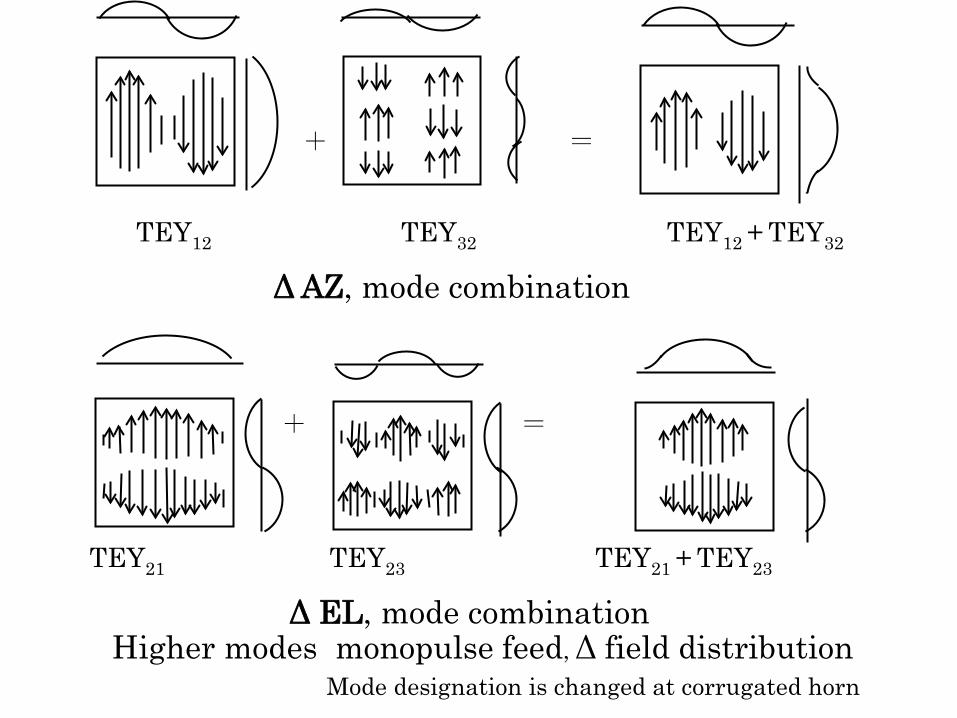
TEY12 TEY32 TEY12 + TEY32

Δ AZ, mode combination

＋ ＝

TEY21 TEY23 TEY21 + TEY23

Δ EL, mode combination Higher modes monopulse feed, Δ field distribution

Mode designation is changed at corrugated horn

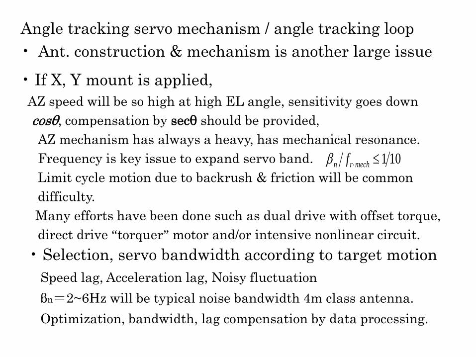
Angle tracking servo mechanism / angle tracking loop • Ant. construction & mechanism is another large issue • If X, Y mount is applied, AZ speed will be so high at high EL angle, sensitivity goes down cosθ, compensation by secθ should be provided, AZ mechanism has always a heavy, has mechanical resonance. Frequency is key issue to expand servo band. Limit cycle motion due to backrush & friction will be common difficulty. Many efforts have been done such as dual drive with offset torque, direct drive “torquer” motor and/or intensive nonlinear circuit. • Selection, servo bandwidth according to target motion

Speed lag, Acceleration lag, Noisy fluctuation βn＝2~6Hz will be typical noise bandwidth 4m class antenna. Optimization, bandwidth, lag compensation by data processing.

101≤⋅mechrn fβ

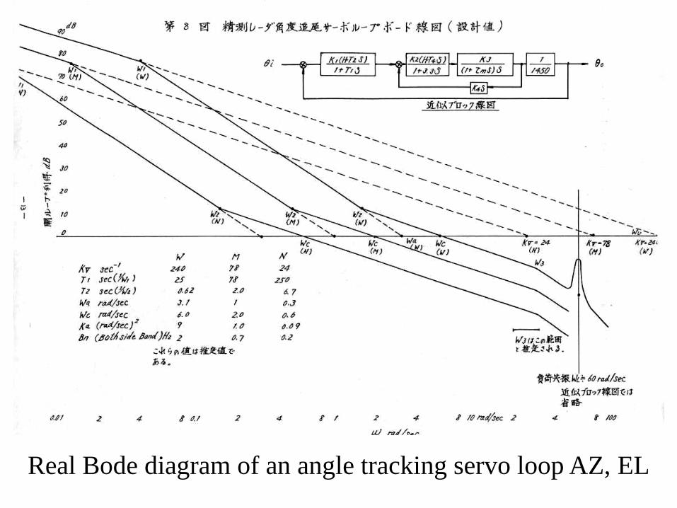
Real Bode diagram of an angle tracking servo loop AZ, EL

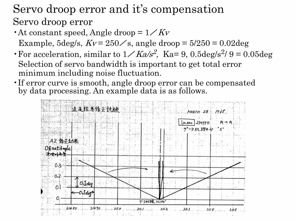
Servo droop error and it’s compensation Servo droop error •At constant speed, Angle droop = 1／Kv Example, 5deg/s, Kv = 250／s, angle droop = 5/250 = 0.02deg •For acceleration, similar to 1／Ka/s2, Ka= 9, 0.5deg/s2/ 9 = 0.05deg Selection of servo bandwidth is important to get total error minimum including noise fluctuation. •If error curve is smooth, angle droop error can be compensated by data processing. An example data is as follows.

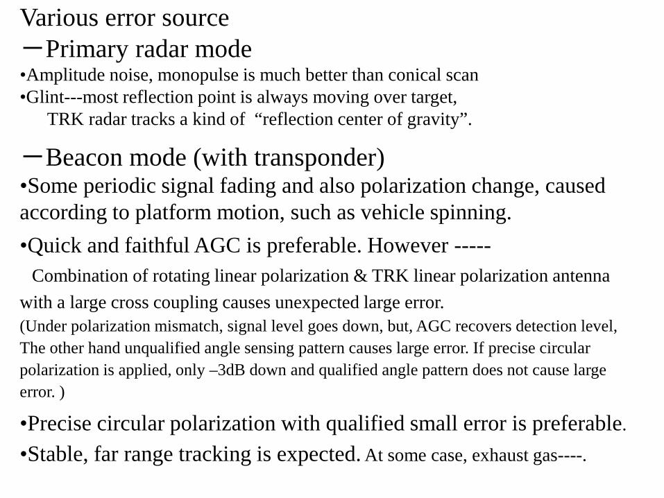
Various error source －Primary radar mode •Amplitude noise, monopulse is much better than conical scan •Glint---most reflection point is always moving over target, TRK radar tracks a kind of “reflection center of gravity”.

－Beacon mode (with transponder) •Some periodic signal fading and also polarization change, caused according to platform motion, such as vehicle spinning. •Quick and faithful AGC is preferable. However ----- Combination of rotating linear polarization & TRK linear polarization antenna with a large cross coupling causes unexpected large error. (Under polarization mismatch, signal level goes down, but, AGC recovers detection level, The other hand unqualified angle sensing pattern causes large error. If precise circular polarization is applied, only –3dB down and qualified angle pattern does not cause large error. )

•Precise circular polarization with qualified small error is preferable.

•Stable, far range tracking is expected. At some case, exhaust gas----.

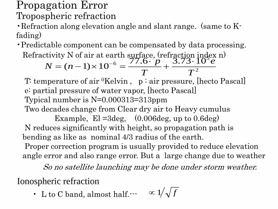
Propagation Error Tropospheric refraction •Refraction along elevation angle and slant range. (same to K-fading) •Predictable component can be compensated by data processing. Refractivity N of air at earth surface, (refraction index n)

T: temperature of air 0Kelvin , p : air pressure, [hecto Pascal] e: partial pressure of water vapor, [hecto Pascal] Typical number is N=0.000313=313ppm Two decades change from Clear dry air to Heavy cumulus Example, El =3deg, (0.006deg, up to 0.6deg) N reduces significantly with height, so propagation path is bending as like as nominal 4/3 radius of the earth. Proper correction program is usually provided to reduce elevation angle error and also range error. But a large change due to weather

So no satellite launching may be done under storm weather.

f1∝• L to C band, almost half.--- Ionospheric refraction

2

56 1073.36.7710)1(

Te

TpnN ⋅+

⋅=×−= −

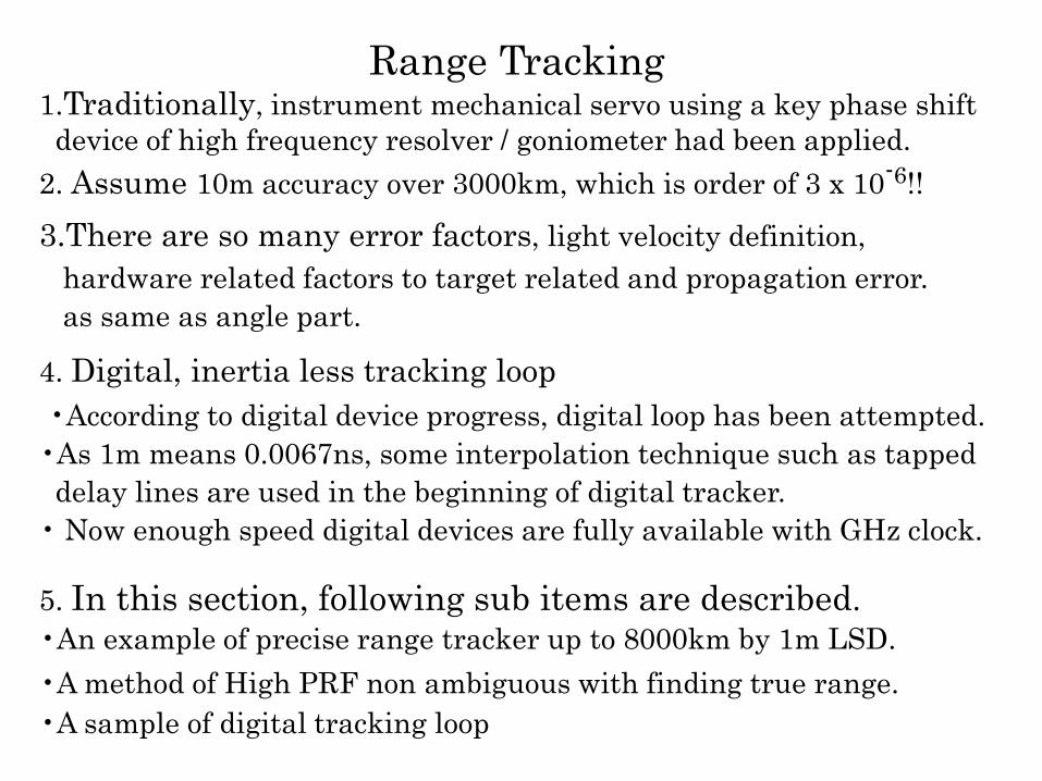
Range Tracking 1.Traditionally, instrument mechanical servo using a key phase shift device of high frequency resolver / goniometer had been applied. 2. Assume 10m accuracy over 3000km, which is order of 3 x 10-6!!

3.There are so many error factors, light velocity definition, hardware related factors to target related and propagation error. as same as angle part.

4. Digital, inertia less tracking loop •According to digital device progress, digital loop has been attempted.

•As 1m means 0.0067ns, some interpolation technique such as tapped delay lines are used in the beginning of digital tracker. • Now enough speed digital devices are fully available with GHz clock.

5. In this section, following sub items are described. •An example of precise range tracker up to 8000km by 1m LSD. •A method of High PRF non ambiguous with finding true range. •A sample of digital tracking loop

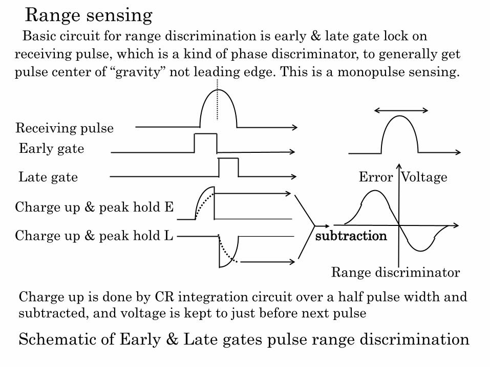
Range sensing Basic circuit for range discrimination is early & late gate lock on receiving pulse, which is a kind of phase discriminator, to generally get pulse center of “gravity” not leading edge. This is a monopulse sensing.

Receiving pulse Early gate

Late gate Error Voltage

Charge up & peak hold E

Charge up & peak hold L subtraction

Range discriminator

Schematic of Early & Late gates pulse range discrimination

Charge up is done by CR integration circuit over a half pulse width and subtracted, and voltage is kept to just before next pulse

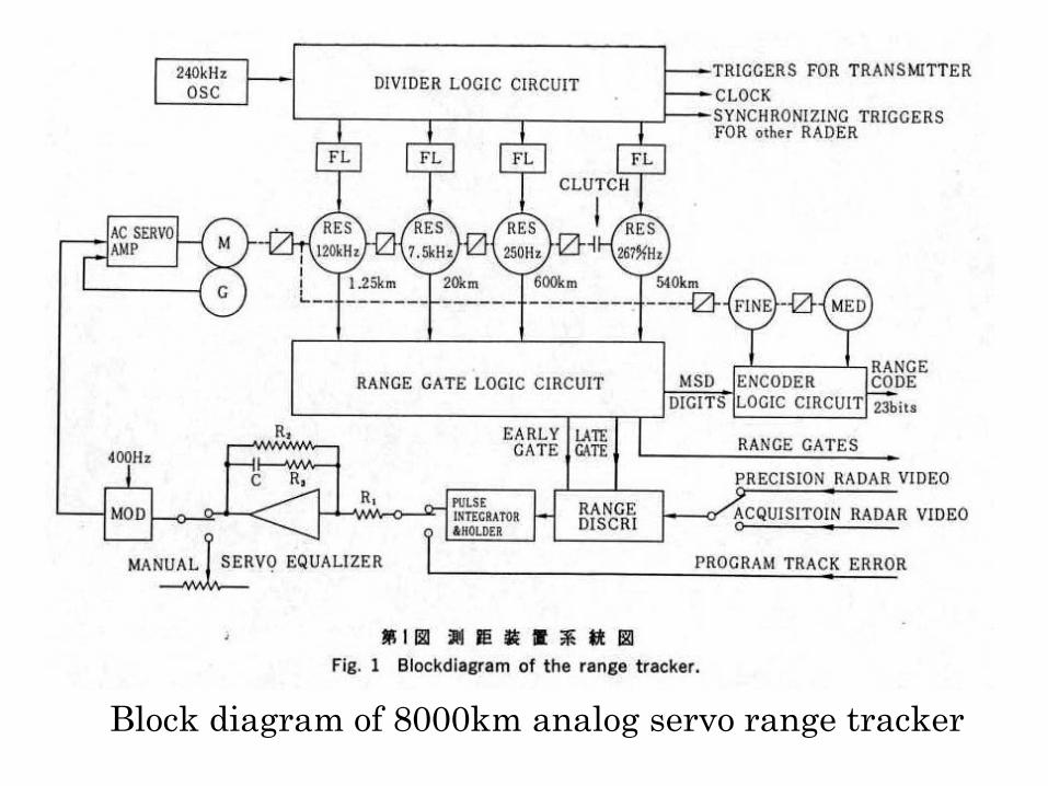
Block diagram of 8000km analog servo range tracker

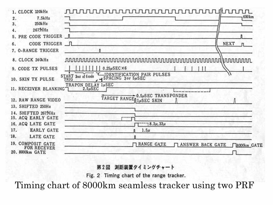
Timing chart of 8000km seamless tracker using two PRF

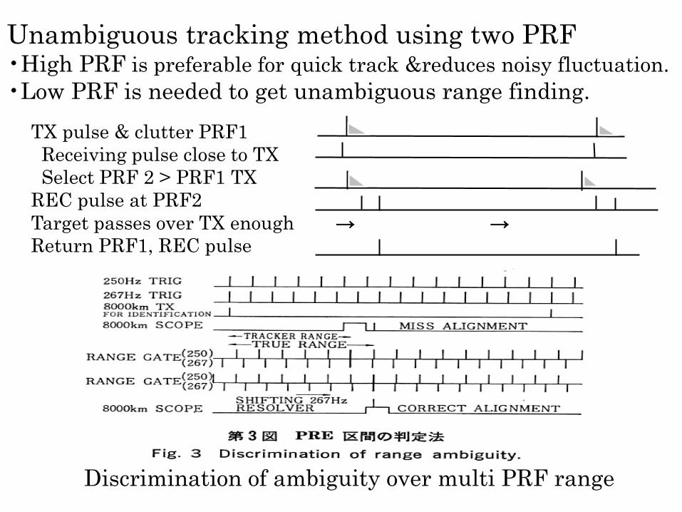
Unambiguous tracking method using two PRF •High PRF is preferable for quick track &reduces noisy fluctuation. •Low PRF is needed to get unambiguous range finding.

TX pulse & clutter PRF1 Receiving pulse close to TX Select PRF 2 > PRF1 TX REC pulse at PRF2 Target passes over TX enough → → Return PRF1, REC pulse

Discrimination of ambiguity over multi PRF range

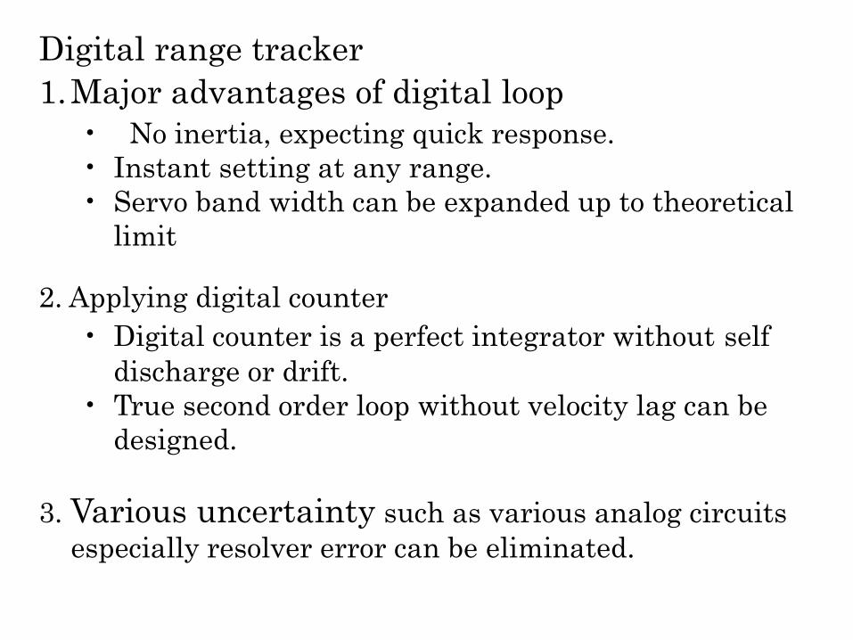
Digital range tracker 1.Major advantages of digital loop

• No inertia, expecting quick response. • Instant setting at any range. • Servo band width can be expanded up to theoretical

limit 2. Applying digital counter

• Digital counter is a perfect integrator without self discharge or drift.

• True second order loop without velocity lag can be designed.

3. Various uncertainty such as various analog circuits

especially resolver error can be eliminated.

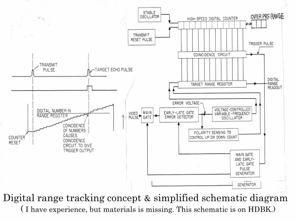
Digital range tracking concept & simplified schematic diagram ( I have experience, but materials is missing. This schematic is on HDBK.)

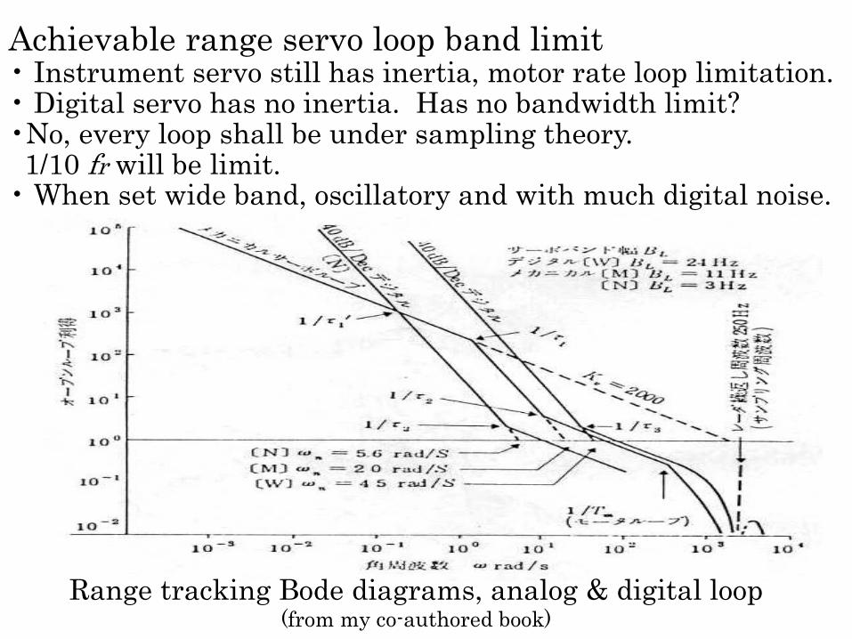
Achievable range servo loop band limit • Instrument servo still has inertia, motor rate loop limitation. • Digital servo has no inertia. Has no bandwidth limit? •No, every loop shall be under sampling theory. 1/10 fr will be limit. • When set wide band, oscillatory and with much digital noise.

Range tracking Bode diagrams, analog & digital loop (from my co-authored book)

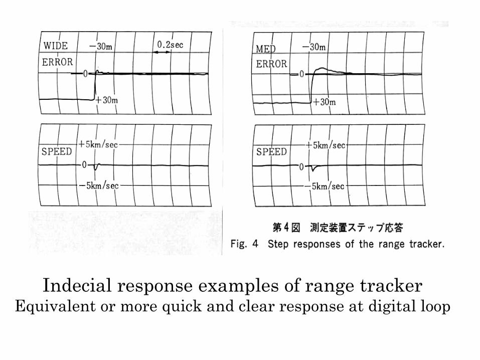
Indecial response examples of range tracker Equivalent or more quick and clear response at digital loop

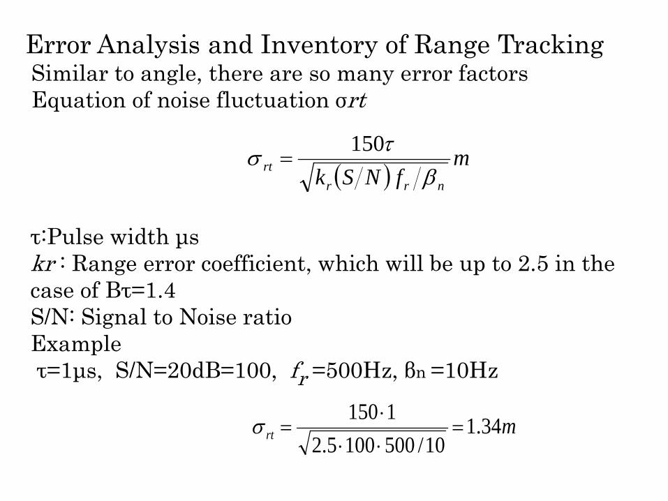
Error Analysis and Inventory of Range Tracking Similar to angle, there are so many error factors Equation of noise fluctuation σrt

( )m

fNSk nrrrt β

τσ 150=

τ:Pulse width μs kr : Range error coefficient, which will be up to 2.5 in the case of Bτ=1.4 S/N: Signal to Noise ratio Example τ=1μs, S/N=20dB=100, fr =500Hz, βn =10Hz

mrt 34.110/5001005.2

1150=

⋅⋅⋅

=σ

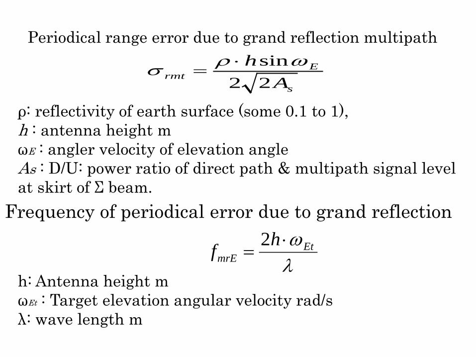
Periodical range error due to grand reflection multipath

ρ: reflectivity of earth surface (some 0.1 to 1), h : antenna height m ωE : angler velocity of elevation angle As : D/U: power ratio of direct path & multipath signal level at skirt of Σ beam.

s

Ermt A

h22sinωρσ ⋅

=

Frequency of periodical error due to grand reflection

λωEt

mrEhf ⋅

=2

h: Antenna height m ωEt : Target elevation angular velocity rad/s λ: wave length m

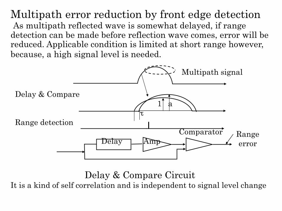
Multipath error reduction by front edge detection As multipath reflected wave is somewhat delayed, if range detection can be made before reflection wave comes, error will be reduced. Applicable condition is limited at short range however, because, a high signal level is needed.

Delay & Compare 1 a τ Range detection Comparator Delay Amp

Multipath signal

Delay & Compare Circuit It is a kind of self correlation and is independent to signal level change

Range error

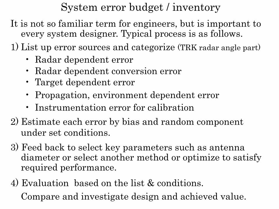
System error budget / inventory It is not so familiar term for engineers, but is important to

every system designer. Typical process is as follows. 1) List up error sources and categorize (TRK radar angle part)

• Radar dependent error • Radar dependent conversion error • Target dependent error • Propagation, environment dependent error • Instrumentation error for calibration

2) Estimate each error by bias and random component under set conditions. 3) Feed back to select key parameters such as antenna

diameter or select another method or optimize to satisfy required performance.

4) Evaluation based on the list & conditions. Compare and investigate design and achieved value.

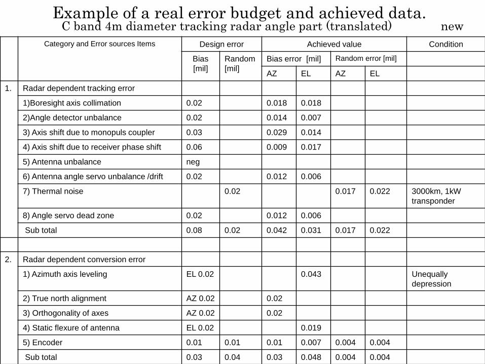
Example of a real error budget and achieved data. C band 4m diameter tracking radar angle part (translated) new

Category and Error sources Items Design error Achieved value Condition

Bias [mil]

Random [mil]

Bias error [mil] Random error [mil]

AZ EL AZ EL

1. Radar dependent tracking error

1)Boresight axis collimation 0.02 0.018 0.018

2)Angle detector unbalance 0.02 0.014 0.007

3) Axis shift due to monopuls coupler 0.03 0.029 0.014

4) Axis shift due to receiver phase shift 0.06 0.009 0.017

5) Antenna unbalance neg

6) Antenna angle servo unbalance /drift 0.02 0.012 0.006

7) Thermal noise 0.02 0.017 0.022 3000km, 1kW transponder

8) Angle servo dead zone 0.02 0.012 0.006

Sub total 0.08 0.02 0.042 0.031 0.017 0.022

2. Radar dependent conversion error

1) Azimuth axis leveling EL 0.02 0.043 Unequally depression

2) True north alignment AZ 0.02 0.02

3) Orthogonality of axes AZ 0.02 0.02

4) Static flexure of antenna EL 0.02 0.019

5) Encoder 0.01 0.01 0.01 0.007 0.004 0.004

Sub total 0.03 0.04 0.03 0.048 0.004 0.004

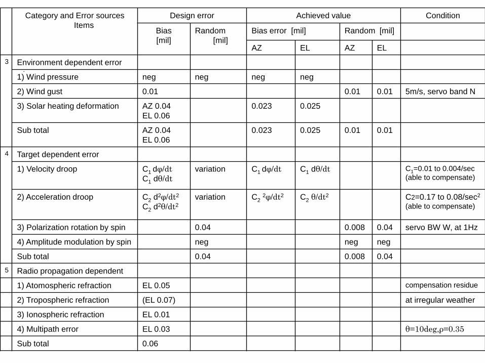
Category and Error sources Items

Design error Achieved value Condition

Bias [mil]

Random [mil]

Bias error [mil] Random [mil]

AZ EL AZ EL 3

. Environment dependent error

1) Wind pressure neg neg neg neg

2) Wind gust 0.01 0.01 0.01 5m/s, servo band N

3) Solar heating deformation AZ 0.04 EL 0.06

0.023 0.025

Sub total AZ 0.04 EL 0.06

0.023 0.025 0.01 0.01

4 Target dependent error

1) Velocity droop C1 dφ/dt C1 dθ/dt

variation

C1 dφ/dt C1 dθ/dt

C1=0.01 to 0.004/sec (able to compensate)

2) Acceleration droop C2 d2φ/dt2 C2 d2θ/dt2

variation C2 2φ/dt2 C2 θ/dt2 C2=0.17 to 0.08/sec2 (able to compensate)

3) Polarization rotation by spin 0.04 0.008 0.04 servo BW W, at 1Hz

4) Amplitude modulation by spin neg neg neg

Sub total 0.04 0.008 0.04 5 Radio propagation dependent 1) Atomospheric refraction EL 0.05 compensation residue

2) Tropospheric refraction (EL 0.07) at irregular weather 3) Ionospheric refraction EL 0.01 4) Multipath error EL 0.03 θ=10deg,ρ=0.35 Sub total 0.06

Closing •All of tracking radar system design is so difficult to explain during a few hours, which contains various engineering fields. Only one engineer can hardly cover all, so a design group by several experts is needed to perform design. •Today, I explained some of tracking radar system design based on my real experience and knowledge of antenna. •I frankly recommend you, when you develop or purchase a tracking radar, you try error budget analysis cycles and evaluation based on it.

-Time change to the future-

Some of tracking radar may be replaced by non mechanical phased array system and GPS navigation & communication.