Machine Learning: Probability Theory

Machine Learning

Probability Theory

WS2013/2014 – Dmitrij Schlesinger, Carsten Rother

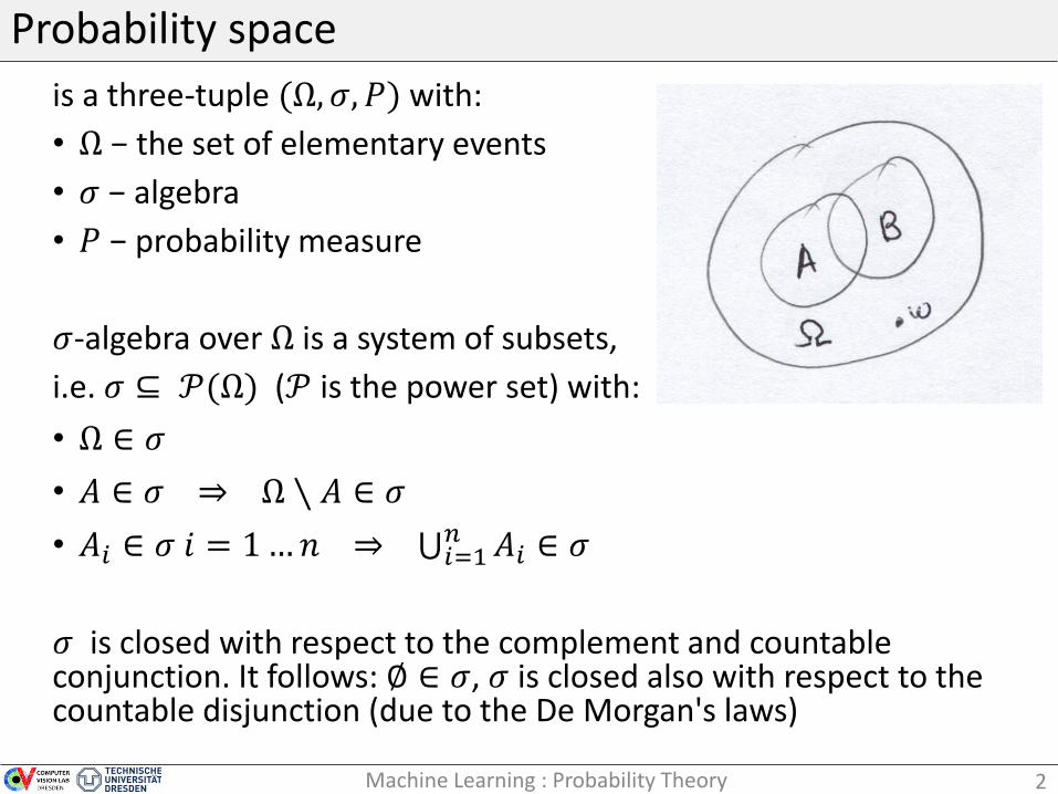
Probability space

is a three-tuple (Ω, 𝜎, 𝑃) with:

• Ω − the set of elementary events

• 𝜎 − algebra

• 𝑃 − probability measure

𝜎-algebra over Ω is a system of subsets,

i.e. 𝜎 ⊆ 𝒫(Ω) (𝒫 is the power set) with:

• Ω ∈ 𝜎

• 𝐴 ∈ 𝜎 ⇒ Ω ∖ 𝐴 ∈ 𝜎

• 𝐴𝑖 ∈ 𝜎 𝑖 = 1…𝑛 ⇒ 𝑖=1𝑛 𝐴𝑖 ∈ 𝜎

𝜎 is closed with respect to the complement and countable conjunction. It follows: ∅ ∈ 𝜎, 𝜎 is closed also with respect to the countable disjunction (due to the De Morgan's laws)

2Machine Learning : Probability Theory

Probability space

Examples:

• 𝜎 = ∅,Ω (smallest) and 𝜎 = 𝒫 Ω (largest) 𝜎-algebras over Ω

• the minimal 𝜎-algebra over Ω containing a particular subset 𝐴 ∈ Ωis 𝜎 = ∅, 𝐴, Ω ∖ 𝐴, Ω

• Ω is discrete and finite, 𝜎 = 2Ω

• Ω = ℝ , the Borel-algebra (contains all intervals among others)

• etc.


Probability measure

𝑃: 𝜎 → 0,1 is a „measure“ (Π) with the normalizing 𝑃 Ω = 1

𝜎-additivity: let 𝐴𝑖 ∈ 𝜎 be pairwise disjoint subsets, i.e. 𝐴𝑖 ∩ 𝐴𝑖′ = ∅, then

𝑃

𝑖

𝐴𝑖 =

𝑖

𝑃(𝐴𝑖)

Note: there are sets for which there is no measure.

Examples: the set of irrational numbers, function spaces ℝ∞ etc.

Banach-Tarski paradoxon (see Wikipedia ):


(For us) practically relevant cases

• The set Ω is „good-natured“, e.g. ℝ𝑛, discrete finite sets etc.

• 𝜎 = 𝒫 Ω , i.e. the algebra is the power set

• We often consider a (composite) „event“ 𝐴 ⊆ Ω as the union of elemantary ones

• Probability of an event is

𝑃 𝐴 =

𝜔∈𝐴

𝑃(𝜔)


Random variables

Here a special case – real-valued random variables.

A random variable 𝜉 for a probability space (Ω, 𝜎, 𝑃) is a mapping 𝜉: Ω → ℝ, satisfying

𝜔: 𝜉 𝜔 ≤ 𝑟 ∈ 𝜎 ∀ 𝑟 ∈ ℝ

(always holds for power sets)

Note: elementary events are not numbers – they are elements of a general set Ω

Random variables are in contrast numbers, i.e. they can be summed up, subtracted, squared etc.


Distributions

Cummulative distribution function of a random variable 𝜉 :

𝐹𝜉 𝑟 = 𝑃 𝜔: 𝜉 𝜔 ≤ 𝑟

Probability distribution of a discrete random variable 𝜉: Ω → ℤ :

𝑝𝜉 𝑟 = 𝑃({𝜔: 𝜉 𝜔 = 𝑟})

Probability density of a continuous random variable 𝜉: Ω → ℝ :

𝑝𝜉 𝑟 =𝜕𝐹𝜉(𝑟)

𝜕𝑟


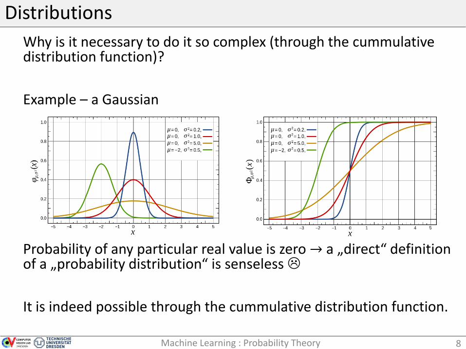
Distributions

Why is it necessary to do it so complex (through the cummulative distribution function)?

Example – a Gaussian

Probability of any particular real value is zero → a „direct“ definition of a „probability distribution“ is senseless

It is indeed possible through the cummulative distribution function.


Mean

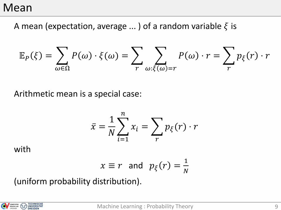
A mean (expectation, average ... ) of a random variable 𝜉 is

𝔼𝑃 𝜉 =

𝜔∈Ω

𝑃 𝜔 ⋅ 𝜉(𝜔) =

𝑟

𝜔:𝜉 𝜔 =𝑟

𝑃 𝜔 ⋅ 𝑟 =

𝑟

𝑝𝜉 𝑟 ⋅ 𝑟

Arithmetic mean is a special case:

𝑥 =1

𝑁

𝑖=1

𝑛

𝑥𝑖 =

𝑟

𝑝𝜉(𝑟) ⋅ 𝑟

with

𝑥 ≡ 𝑟 and 𝑝𝜉 𝑟 =1

𝑁

(uniform probability distribution).


Mean

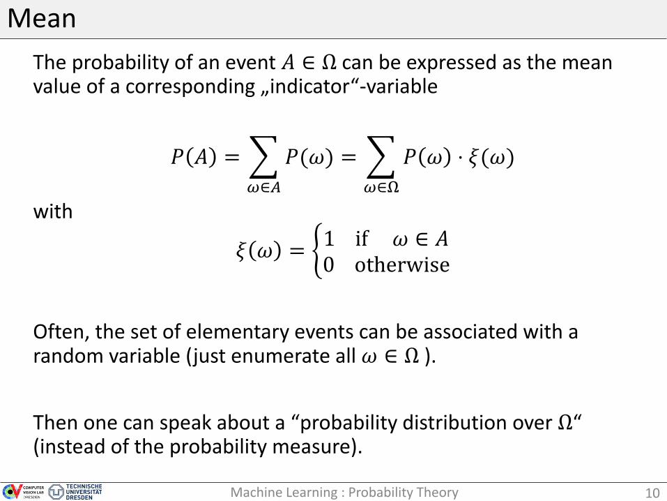
The probability of an event 𝐴 ∈ Ω can be expressed as the mean value of a corresponding „indicator“-variable

𝑃 𝐴 =

𝜔∈𝐴

𝑃(𝜔) =

𝜔∈Ω

𝑃 𝜔 ⋅ 𝜉(𝜔)

with

𝜉 𝜔 = 1 if 𝜔 ∈ 𝐴0 otherwise

Often, the set of elementary events can be associated with a random variable (just enumerate all 𝜔 ∈ Ω ).

Then one can speak about a “probability distribution over Ω“ (instead of the probability measure).


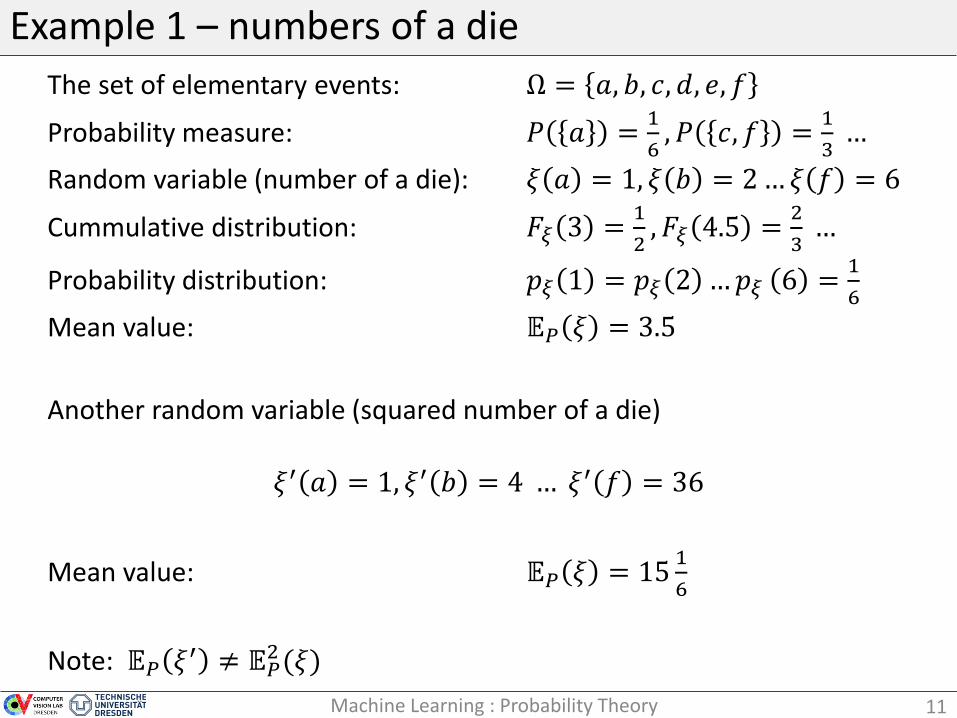
Example 1 – numbers of a die

The set of elementary events: Ω = 𝑎, 𝑏, 𝑐, 𝑑, 𝑒, 𝑓

Probability measure: 𝑃 𝑎 =1

6, 𝑃 𝑐, 𝑓 =

1

3…

Random variable (number of a die): 𝜉 𝑎 = 1, 𝜉 𝑏 = 2…𝜉 𝑓 = 6

Cummulative distribution: 𝐹𝜉 3 =1

2, 𝐹𝜉 4.5 =

2

3…

Probability distribution: 𝑝𝜉 1 = 𝑝𝜉 2 …𝑝𝜉 6 =1

6

Mean value: 𝔼𝑃 𝜉 = 3.5

Another random variable (squared number of a die)

𝜉′ 𝑎 = 1, 𝜉′ 𝑏 = 4 … 𝜉′ 𝑓 = 36

Mean value: 𝔼𝑃 𝜉 = 151

6

Note: 𝔼𝑃 𝜉′ ≠ 𝔼𝑃2(𝜉)


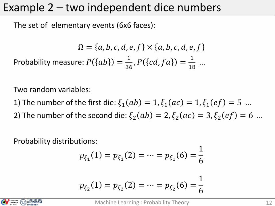
Example 2 – two independent dice numbers

The set of elementary events (6x6 faces):

Ω = 𝑎, 𝑏, 𝑐, 𝑑, 𝑒, 𝑓 × 𝑎, 𝑏, 𝑐, 𝑑, 𝑒, 𝑓

Probability measure: 𝑃 𝑎𝑏 =1

36, 𝑃 𝑐𝑑, 𝑓𝑎 =

1

18…

Two random variables:

1) The number of the first die: 𝜉1 𝑎𝑏 = 1, 𝜉1 𝑎𝑐 = 1, 𝜉1 𝑒𝑓 = 5 …

2) The number of the second die: 𝜉2 𝑎𝑏 = 2, 𝜉2 𝑎𝑐 = 3, 𝜉2 𝑒𝑓 = 6 …

Probability distributions:

𝑝𝜉1 1 = 𝑝𝜉1 2 = ⋯ = 𝑝𝜉1 6 =1

6

𝑝𝜉2 1 = 𝑝𝜉2 2 = ⋯ = 𝑝𝜉2 6 =1

6


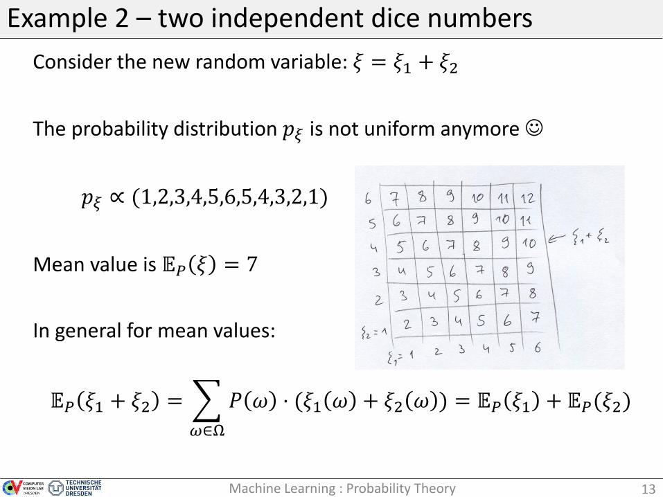
Example 2 – two independent dice numbers

Consider the new random variable: 𝜉 = 𝜉1 + 𝜉2

The probability distribution 𝑝𝜉 is not uniform anymore

𝑝𝜉 ∝ (1,2,3,4,5,6,5,4,3,2,1)

Mean value is 𝔼𝑃 𝜉 = 7

In general for mean values:

𝔼𝑃 𝜉1 + 𝜉2 =

𝜔∈Ω

𝑃 𝜔 ⋅ (𝜉1 𝜔 + 𝜉2 𝜔 ) = 𝔼𝑃 𝜉1 + 𝔼𝑃(𝜉2)


Random variables of higher dimension

Analogously: Let 𝜉: Ω → ℝ𝑛 be a mapping (𝑛 = 2 for simplicity), with 𝜉 = 𝜉1, 𝜉2 , 𝜉1: Ω → ℝ and 𝜉2: Ω → ℝ

Cummulative distribution function:

𝐹𝜉 𝑟, 𝑠 = 𝑃 𝜔: 𝜉1 𝜔 ≤ 𝑟 ∩ 𝜔: 𝜉2 𝜔 ≤ 𝑠

Joint probability distribution (discrete):

𝑝𝜉= 𝜉1,𝜉2 𝑟, 𝑠 = 𝑃 𝜔: 𝜉1 𝜔 = 𝑟 ∩ 𝜔: 𝜉2 𝜔 = 𝑠

Joint probability density (continuous):

𝑝𝜉= 𝜉1,𝜉2 𝑟, 𝑠 =𝜕2𝐹𝜉(𝑟, 𝑠)

𝜕𝑟 𝜕𝑠14Machine Learning : Probability Theory

Independence

Two events 𝐴 ∈ 𝜎 and 𝐵 ∈ 𝜎 are independent, if

𝑃 𝐴 ∩ 𝐵 = 𝑃 𝐴 ⋅ 𝑃(𝐵)

Interesting: Events 𝐴 and 𝐵 = Ω ∖ 𝐵 are independent, if 𝐴 and 𝐵 are independent

Two random variables are independent, if

𝐹𝜉= 𝜉1,𝜉2 𝑟, 𝑠 = 𝐹𝜉1 𝑟 ⋅ 𝐹𝜉2 𝑠 ∀ 𝑟, 𝑠

It follows (example for continuous 𝜉):

𝑝𝜉 𝑟, 𝑠 =𝜕2𝐹𝜉(𝑟, 𝑠)

𝜕𝑟𝜕𝑠=

𝜕𝐹𝜉1(𝑟)

𝜕𝑟⋅𝜕𝐹𝜉2 𝑠

𝜕𝑠= 𝑝𝜉1 𝑟 ⋅ 𝑝𝜉2 𝑠


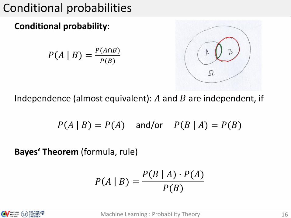
Conditional probabilities

Conditional probability:

𝑃 𝐴 𝐵) =𝑃(𝐴∩𝐵)

𝑃(𝐵)

Independence (almost equivalent): 𝐴 and 𝐵 are independent, if

𝑃 𝐴 𝐵) = 𝑃(𝐴) and/or 𝑃 𝐵 𝐴) = 𝑃(𝐵)

Bayes‘ Theorem (formula, rule)

𝑃 𝐴 𝐵) =𝑃 𝐵 𝐴) ⋅ 𝑃(𝐴)

𝑃(𝐵)


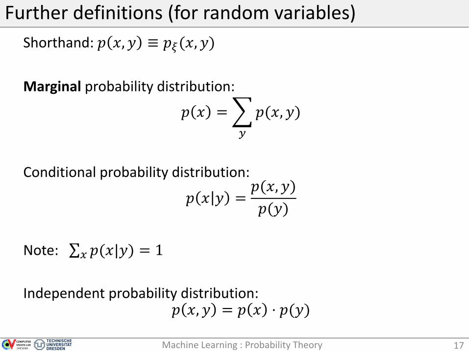
Further definitions (for random variables)

Shorthand: 𝑝 𝑥, 𝑦 ≡ 𝑝𝜉(𝑥, 𝑦)

Marginal probability distribution:

𝑝 𝑥 =

𝑦

𝑝(𝑥, 𝑦)

Conditional probability distribution:

𝑝 𝑥 𝑦 =𝑝(𝑥, 𝑦)

𝑝(𝑦)

Note: 𝑥 𝑝(𝑥|𝑦) = 1

Independent probability distribution:𝑝 𝑥, 𝑦 = 𝑝 𝑥 ⋅ 𝑝(𝑦)


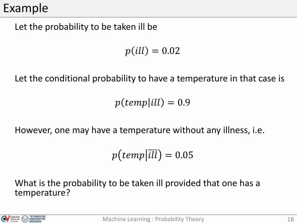
Example

Let the probability to be taken ill be

𝑝 𝑖𝑙𝑙 = 0.02

Let the conditional probability to have a temperature in that case is

𝑝 𝑡𝑒𝑚𝑝 𝑖𝑙𝑙 = 0.9

However, one may have a temperature without any illness, i.e.

𝑝 𝑡𝑒𝑚𝑝 𝑖𝑙𝑙 = 0.05

What is the probability to be taken ill provided that one has a temperature?


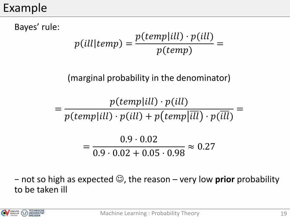
Example

Bayes’ rule:

𝑝 𝑖𝑙𝑙 𝑡𝑒𝑚𝑝 =𝑝 𝑡𝑒𝑚𝑝 𝑖𝑙𝑙 ⋅ 𝑝(𝑖𝑙𝑙)

𝑝(𝑡𝑒𝑚𝑝)=

(marginal probability in the denominator)

=𝑝 𝑡𝑒𝑚𝑝 𝑖𝑙𝑙 ⋅ 𝑝(𝑖𝑙𝑙)

𝑝 𝑡𝑒𝑚𝑝 𝑖𝑙𝑙 ⋅ 𝑝 𝑖𝑙𝑙 + 𝑝 𝑡𝑒𝑚𝑝 𝑖𝑙𝑙 ⋅ 𝑝(𝑖𝑙𝑙)=

=0.9 ⋅ 0.02

0.9 ⋅ 0.02 + 0.05 ⋅ 0.98≈ 0.27

− not so high as expected , the reason – very low prior probabilityto be taken ill


Further topics

The model

Let two random variables be given:

• The first one is typically discrete (i.e. 𝑘 ∈ 𝐾) and is called “class”

• The second one is often continuous (𝑥 ∈ 𝑋) and is called “observation”

Let the joint probability distribution 𝑝(𝑥, 𝑘) be “given”.

As 𝑘 is discrete it is often specified by 𝑝 𝑥, 𝑘 = 𝑝 𝑘 ⋅ 𝑝(𝑥|𝑘)

The recognition task: given 𝑥, estimate 𝑘.

Usual problems (questions):

• How to estimate 𝑘 from 𝑥 ?

• The joint probability is not always explicitly specified.

• The set 𝐾 is sometimes huge.


Further topics

The learning task:

Often (almost always) the probability distribution is known up to free parameters. How to choose them (learn from examples)?

Next classes:

1. Recognition, Bayessian Decision Theory

2. Probabilistic learning, Maximum-Likelihood principle

3. Discriminative models, recognition and learning

…


Documents

Machine Learning: Probability Theory