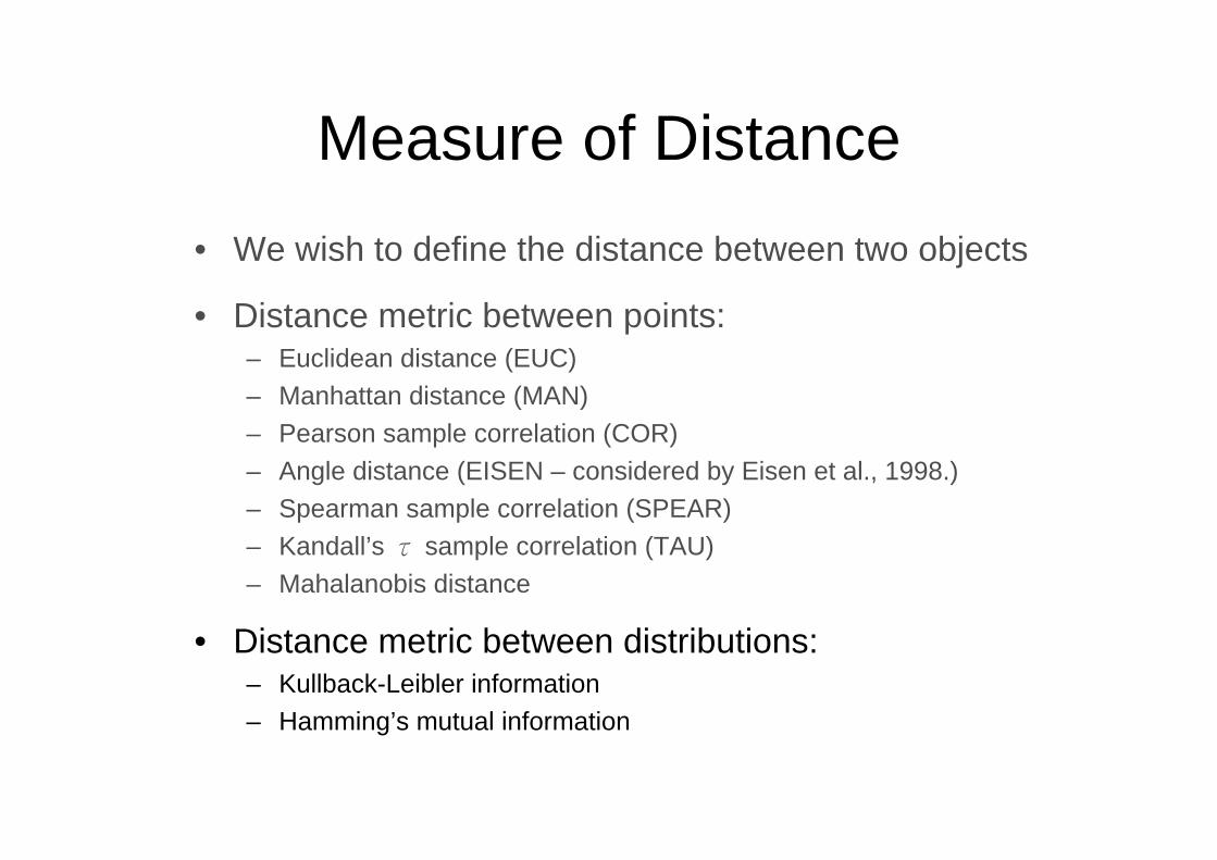
Measure of Distance• We wish to define the distance between two objects

• Distance metric between points:– Euclidean distance (EUC)– Manhattan distance (MAN)– Pearson sample correlation (COR)– Angle distance (EISEN – considered by Eisen et al., 1998.)– Spearman sample correlation (SPEAR)– Kandall’s τ sample correlation (TAU)– Mahalanobis distance

• Distance metric between distributions:– Kullback-Leibler information– Hamming’s mutual information

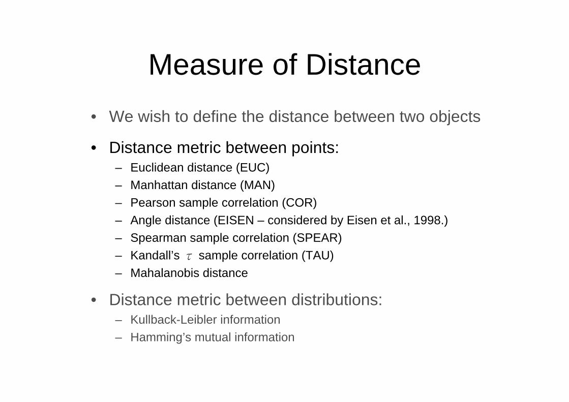
R: Distance Metric Between Points

“dist” function in stat package: – Euclidean– Manhattan

hopach package:– disscosangle(X, na.rm = TRUE) **

bioDist package:– cor.dist– spearman.dist– tau.dist

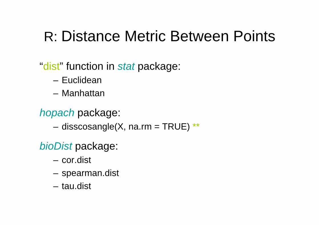
2.07) 1.60,- 1.51,g0.29) 0.75,- 0.04,g0.33) 1.45,- (-1.76,g

3

2

1

((

===

Euclidean distance:

2.45

g2

3.70g3

1.93g2

g1

45.2)29.007.2())75.0(60.1()04.051.1(

70.3)07.233.0())60.1(45.1()51.176.1(

93.1)29.033.0())75.0(45.1()04.076.1(

222

222

222

=−+−−−+−

=−+−−−+−−

=−+−−−+−−

:g3 vs g2

:g3 vs g1

:g2 vs g1

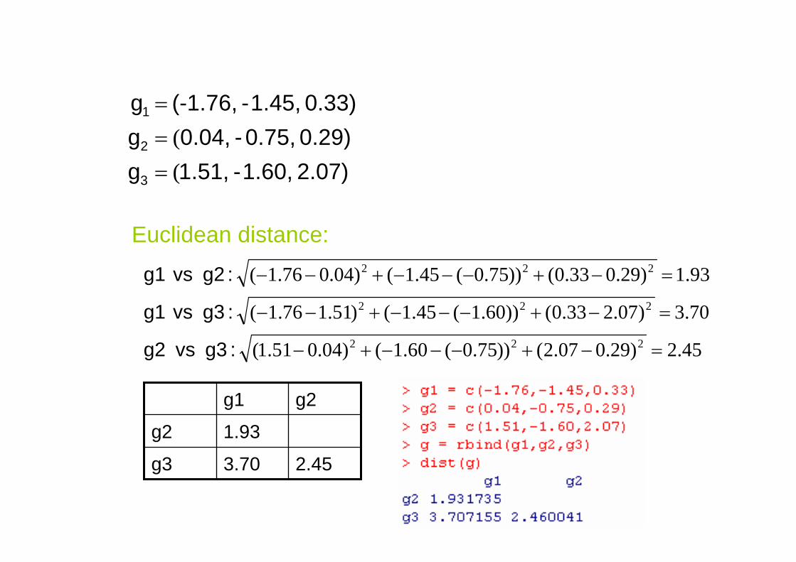
2.07) 1.60,- 1.51,g0.29) 0.75,- 0.04,g0.33) 1.45,- (-1.76,g

3

2

1

((

===

Manhattan distance:

4.10

g2

5.16g3

2.54g2

g1

10.407.2290)60.1(75.0|51.104.016.507.2330)60.1(451|51.1761542290330)750(451040761

=−+−+−=−+−+−=−+−+−

|.||-|-||.||-.|-.|-

.| ..||.-.|-|..|-

:g3 vs g2 :g3 vs g1 :g2 vs g1

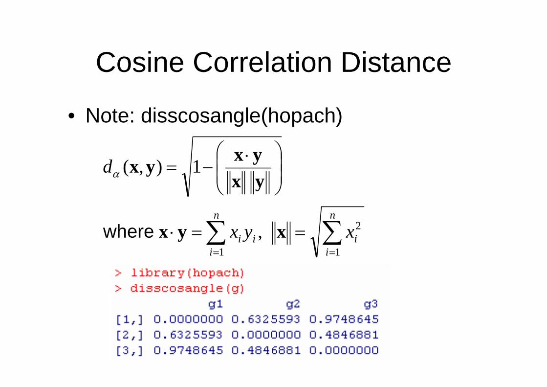
Cosine Correlation Distance

• Note: disscosangle(hopach)

∑∑==

==⋅

⎟⎟⎠

⎞⎜⎜⎝

⎛ ⋅−=

n

ii

n

iii xyx

d

1

2

1,

1),(

xyx

yxyxyx

where

α

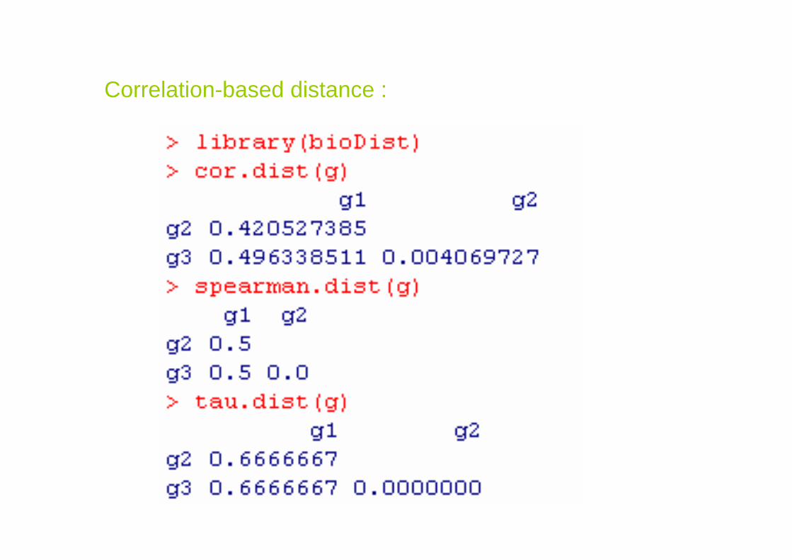
Correlation-based distance :

Measure of Distance• We wish to define the distance between two objects

• Distance metric between points:– Euclidean distance (EUC)– Manhattan distance (MAN)– Pearson sample correlation (COR)– Angle distance (EISEN – considered by Eisen et al., 1998.)– Spearman sample correlation (SPEAR)– Kandall’s τ sample correlation (TAU)– Mahalanobis distance

• Distance metric between distributions:– Kullback-Leibler information– Hamming’s mutual information

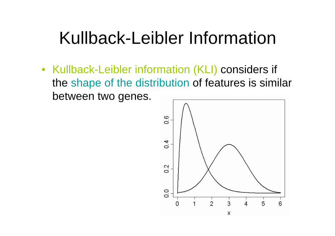
Kullback-Leibler Information

• Kullback-Leibler information (KLI) considers if the shape of the distribution of features is similar between two genes.

f1(x)

f2(x)

Kullback-Leibler Information

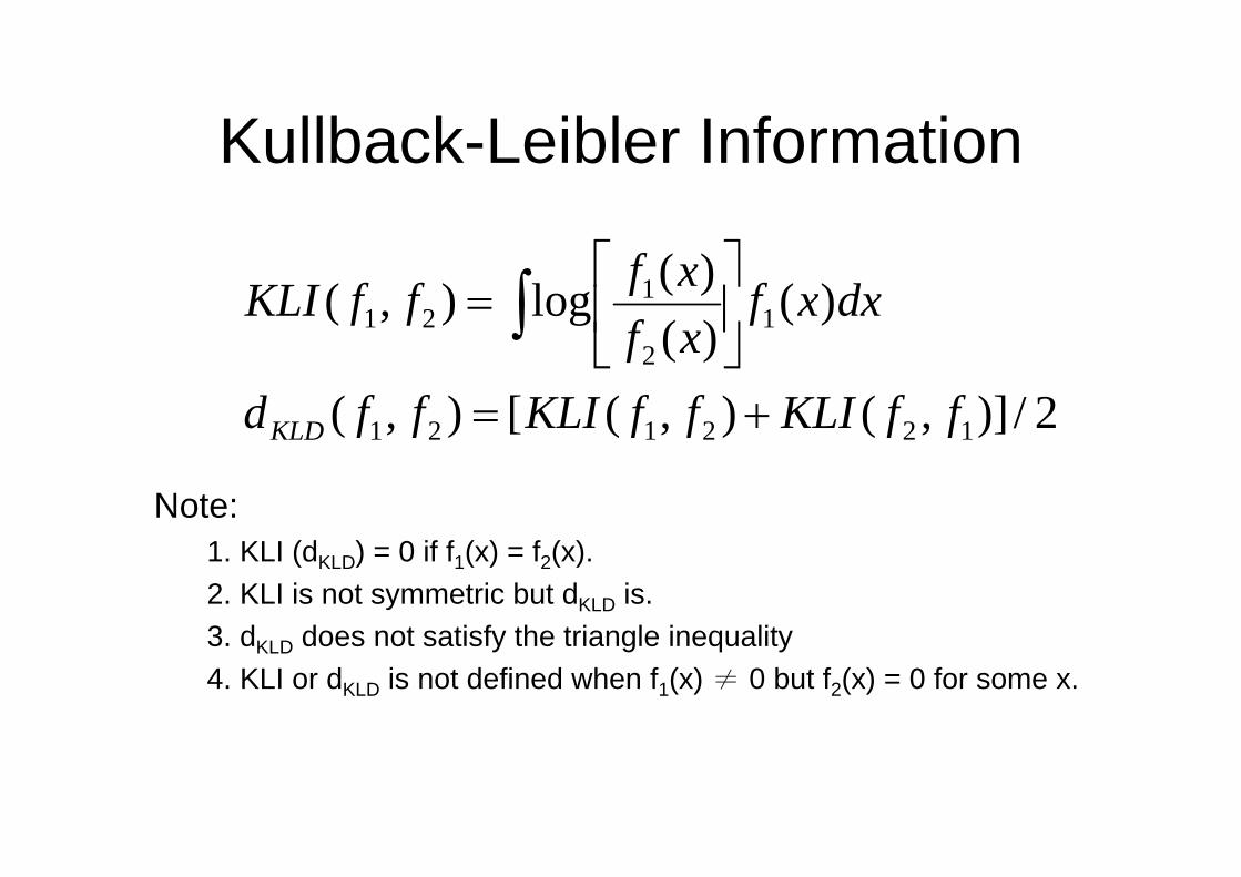
Note: 1. KLI (dKLD) = 0 if f1(x) = f2(x).2. KLI is not symmetric but dKLD is. 3. dKLD does not satisfy the triangle inequality4. KLI or dKLD is not defined when f1(x) ≠ 0 but f2(x) = 0 for some x.

2/)],(),([),(

)()()(log),(

122121

12

121

ffKLIffKLIffd

dxxfxfxfffKLI

KLD +=

⎥⎦

⎤⎢⎣

⎡= ∫

Mutual Information

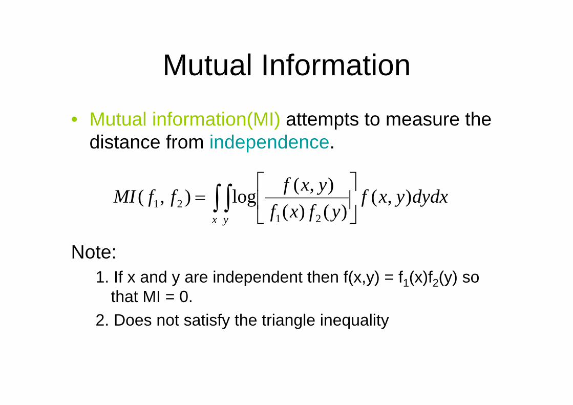
• Mutual information(MI) attempts to measure the distance from independence.

Note:1. If x and y are independent then f(x,y) = f1(x)f2(y) so

that MI = 0.2. Does not satisfy the triangle inequality

∫ ∫ ⎥⎦

⎤⎢⎣

⎡=

x y

dydxyxfyfxf

yxfffMI ),()()(

),(log),(21

21

Mutual Information

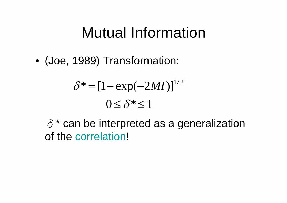
• (Joe, 1989) Transformation:

δ* can be interpreted as a generalization of the correlation!

1*0)]2exp(1[* 2/1

≤≤−−=

δδ MI

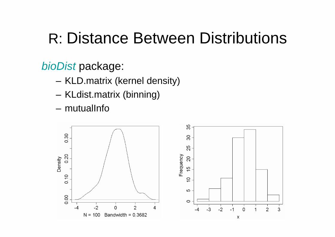
R: Distance Between DistributionsbioDist package:

– KLD.matrix (kernel density)– KLdist.matrix (binning)– mutualInfo

Exercise: Apop.xlshttp://homepage.ntu.edu.tw/~lyliu/IntroBioinfo/Apop.xlsTry to compute the distances between the rows (genes).

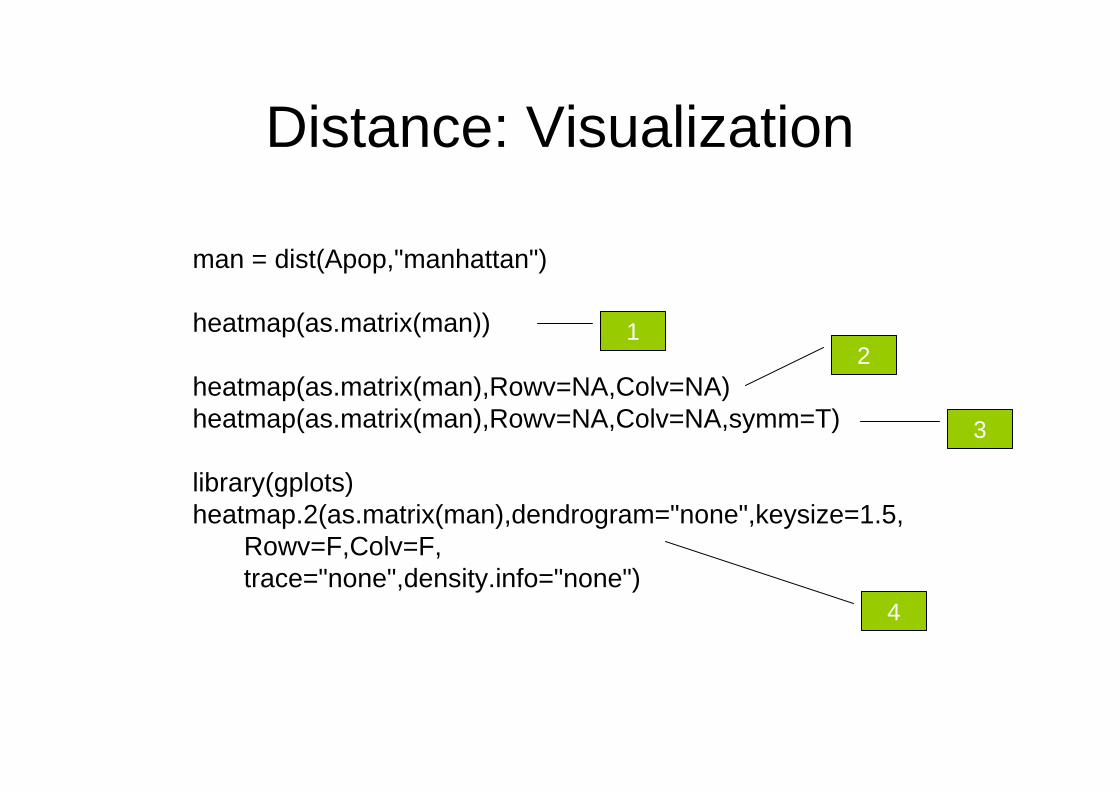
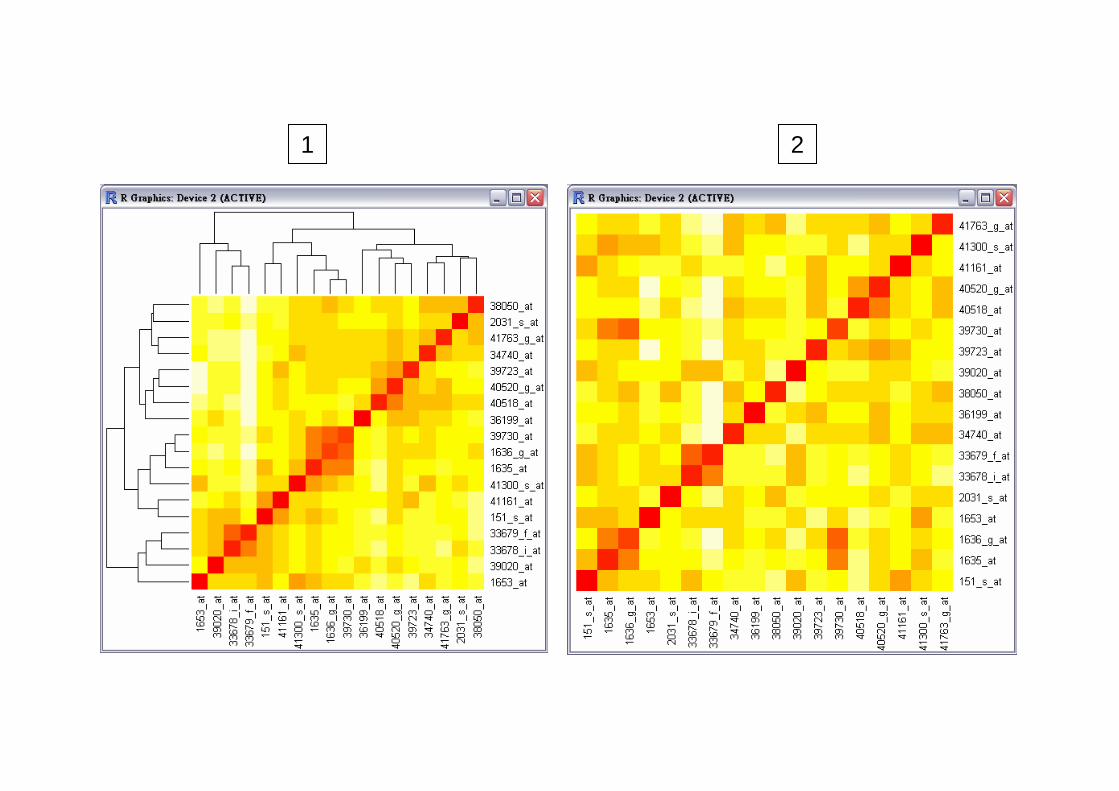
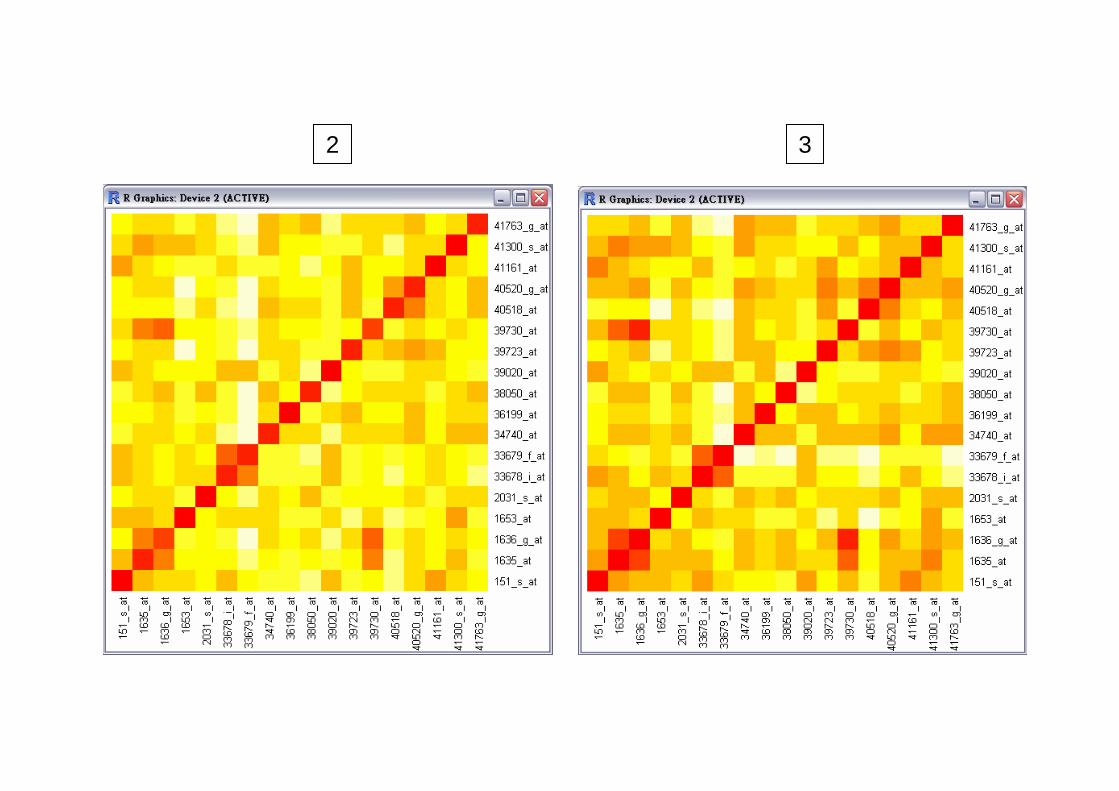
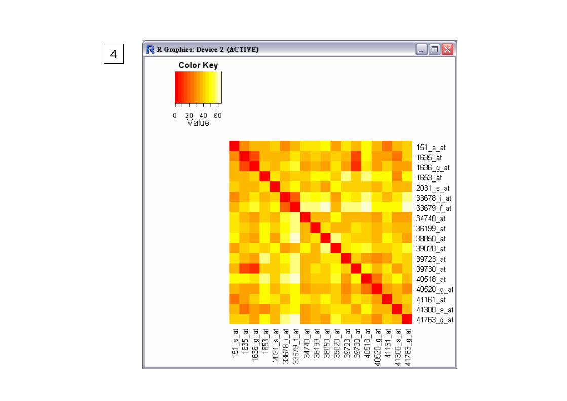
Distance: Visualization

man = dist(Apop,"manhattan")

heatmap(as.matrix(man))

heatmap(as.matrix(man),Rowv=NA,Colv=NA)heatmap(as.matrix(man),Rowv=NA,Colv=NA,symm=T)

library(gplots)heatmap.2(as.matrix(man),dendrogram="none",keysize=1.5,

Rowv=F,Colv=F,trace="none",density.info="none")

12

3

4

1 2

2 3

4

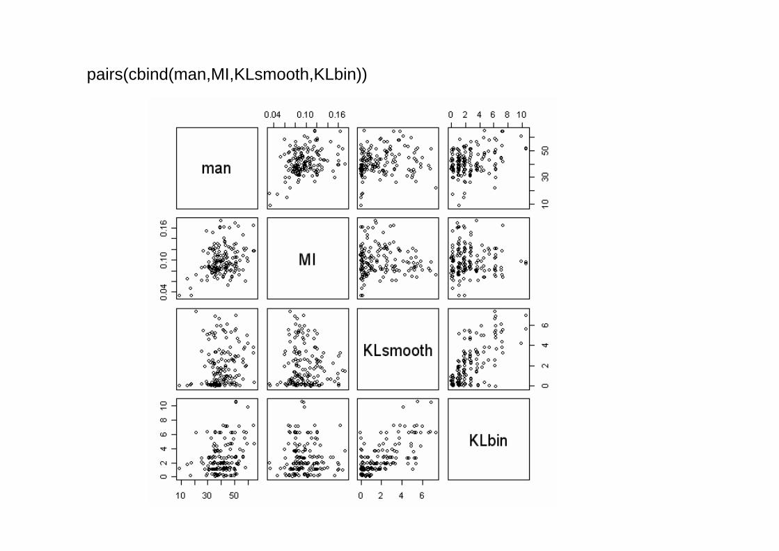
pairs(cbind(man,MI,KLsmooth,KLbin))

Cluster Analysis

• Clustering is the process of grouping grouping togethertogether similar entities. – It is appropriate when there is no prior

knowledge about the data.

– In a machine learning framework, it is known as unsupervised learning since there is no known desired answer for any particular geneor experiment.

Cluster Analysis

• The entities that are similar to each other are grouping together and form a cluster.

– Step 1: Defining the similarity between entities distance metric

– Step 2: Forming clusters clustering algorithms

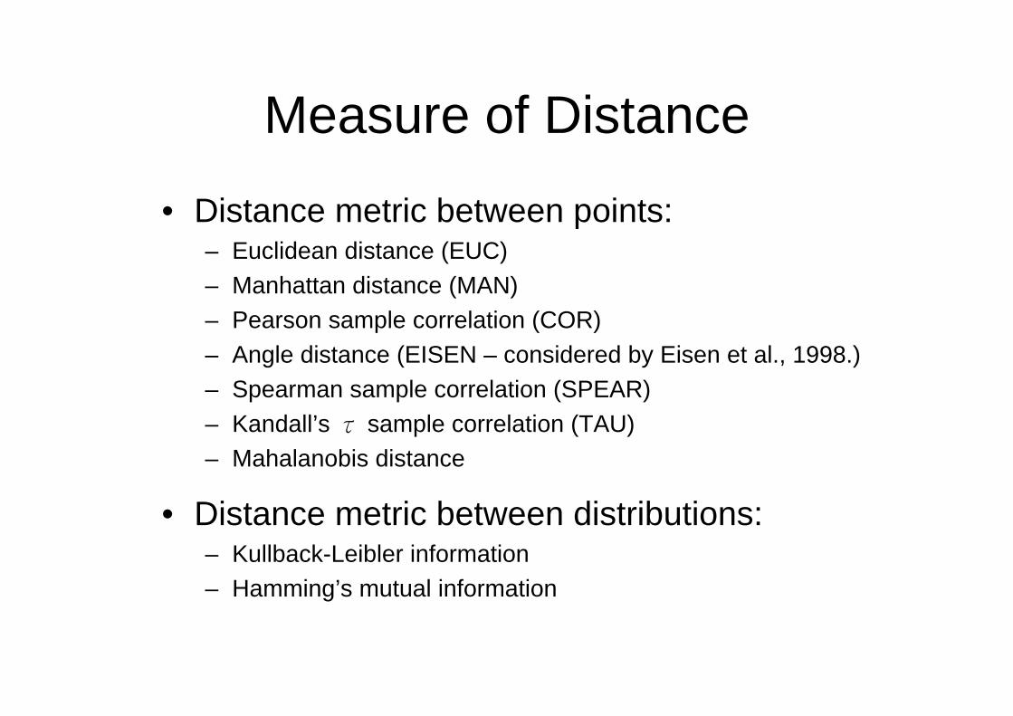
Measure of Distance

• Distance metric between points:– Euclidean distance (EUC)– Manhattan distance (MAN)– Pearson sample correlation (COR)– Angle distance (EISEN – considered by Eisen et al., 1998.)– Spearman sample correlation (SPEAR)– Kandall’s τ sample correlation (TAU)– Mahalanobis distance

• Distance metric between distributions:– Kullback-Leibler information– Hamming’s mutual information

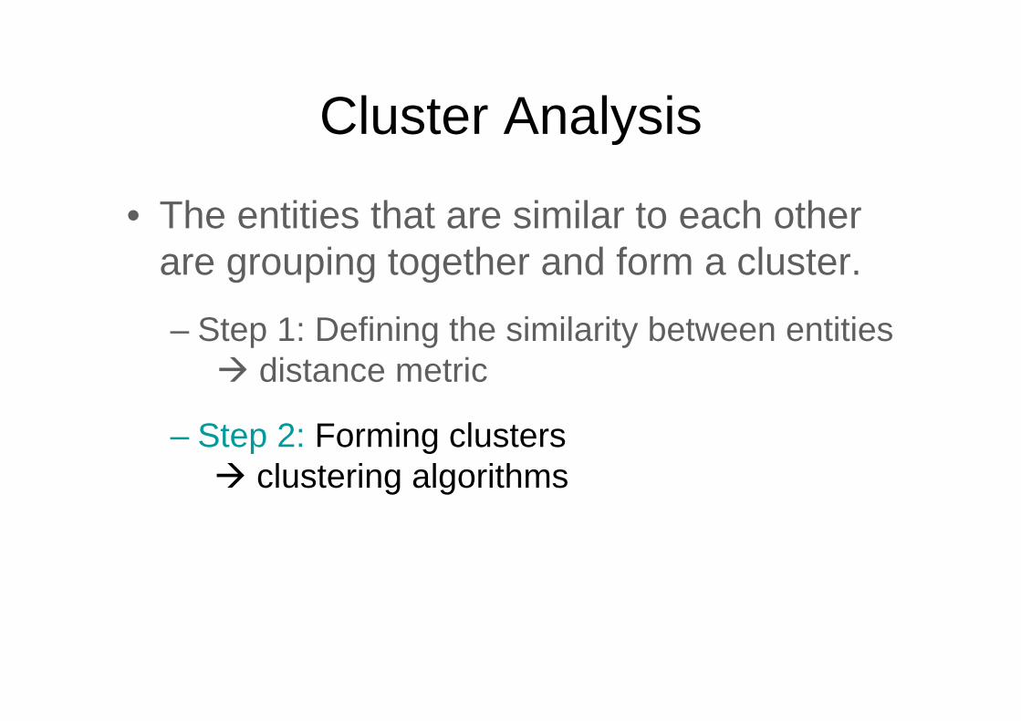
Cluster Analysis

• The entities that are similar to each other are grouping together and form a cluster.

– Step 1: Defining the similarity between entities distance metric

– Step 2: Forming clusters clustering algorithms

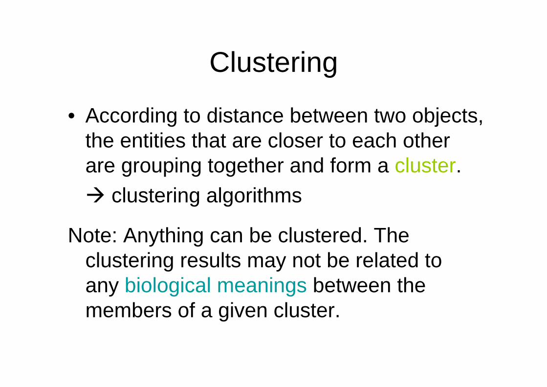
Clustering

• According to distance between two objects, the entities that are closer to each other are grouping together and form a cluster.

clustering algorithms

Note: Anything can be clustered. The clustering results may not be related to any biological meanings between the members of a given cluster.

Clustering

• Usually the results of clustering is shown in a clustering tree, or a dendrogram.

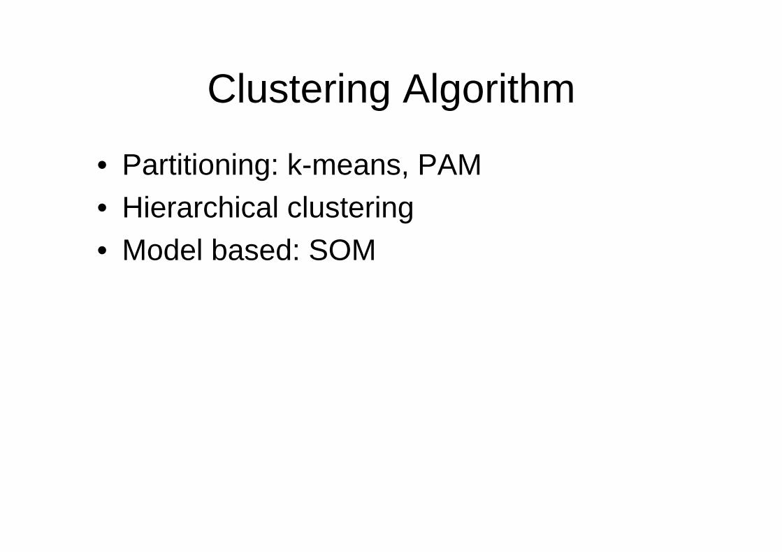
Clustering Algorithm

• Partitioning: k-means, PAM • Hierarchical clustering • Model based: SOM

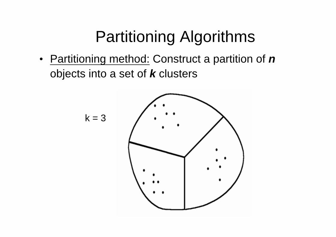
Partitioning Algorithms• Partitioning method: Construct a partition of n

objects into a set of k clusters

k = 3

Partitioning Algorithms

• Given a k, find a partition of k clusters that optimizes the chosen partitioning criterion

– k-means: Each cluster is represented by the center of the cluster

– k-medoids or PAM (Partition around medoids):Each cluster is represented by one of the objects in the cluster

K-means Clustering

Step 1: Determine the number of clusters, k.

Step 2: Randomly choose k point as the centers of clusters.

Step 3: Calculate the distance from each pattern to kcenters and associate every object with the closest cluster center.

Step 4: Calculate a new center for the updated clusters.

Step 5: Repeat steps 3 and 4 until no objects are relocated.

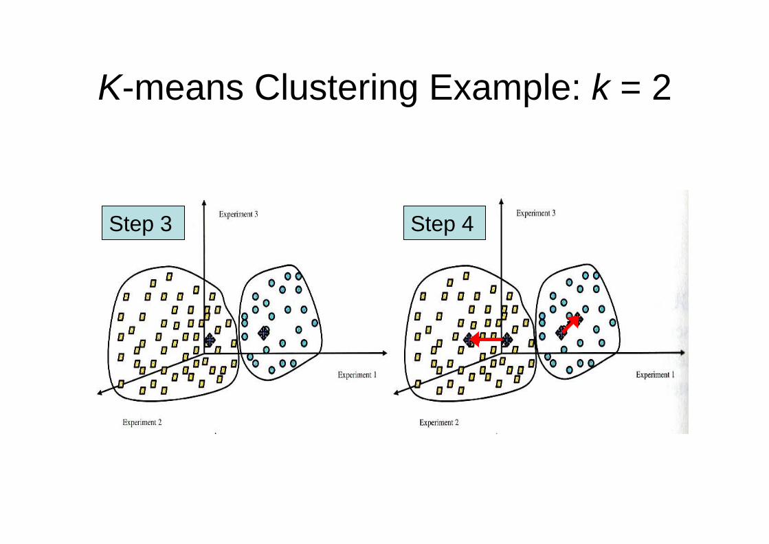
K-means Clustering Example: k = 2

Step 3 Step 4

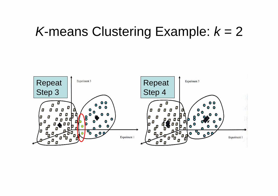
K-means Clustering Example: k = 2

Repeat Step 3

Repeat Step 4

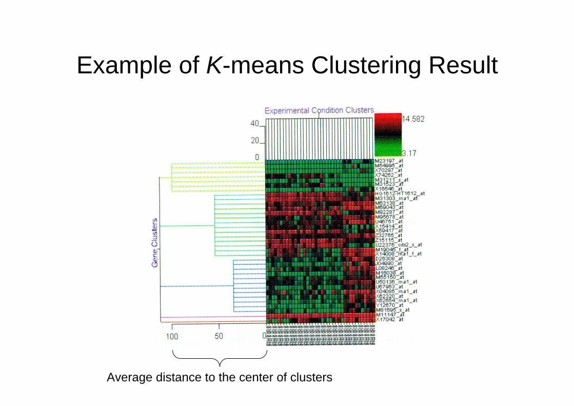
Example of K-means Clustering Result

Average distance to the center of clusters

k-mean Clustering: Properties

1. It is possible to produce empty clusters. To avoid such situation, one can:

(i) let the starting cluster centers be in the general area populated by the given data.

(ii) randomly choose k points as initial centers.

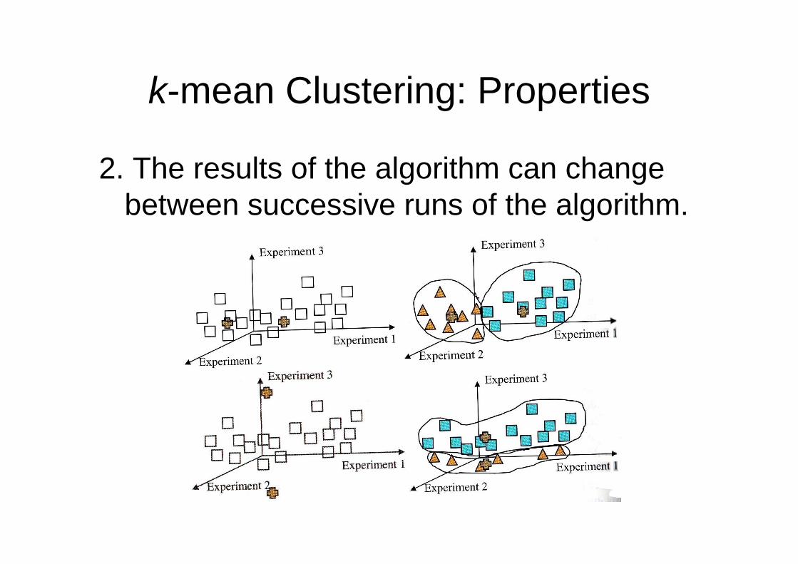
k-mean Clustering: Properties

2. The results of the algorithm can change between successive runs of the algorithm.

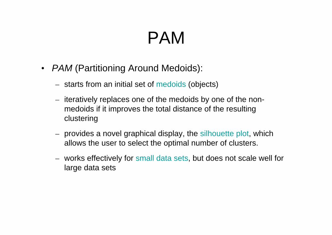
PAM• PAM (Partitioning Around Medoids):

– starts from an initial set of medoids (objects)

– iteratively replaces one of the medoids by one of the non-medoids if it improves the total distance of the resulting clustering

– provides a novel graphical display, the silhouette plot, which allows the user to select the optimal number of clusters.

– works effectively for small data sets, but does not scale well for large data sets

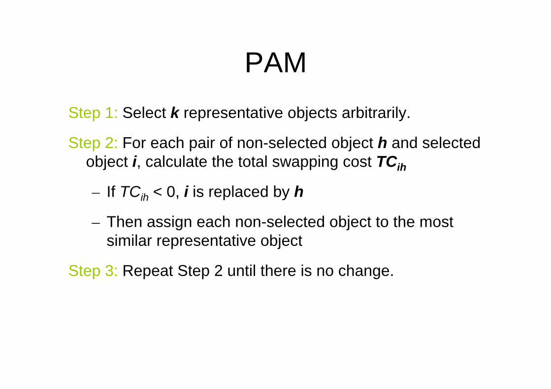
PAMStep 1: Select k representative objects arbitrarily.

Step 2: For each pair of non-selected object h and selected object i, calculate the total swapping cost TCih

– If TCih < 0, i is replaced by h

– Then assign each non-selected object to the most similar representative object

Step 3: Repeat Step 2 until there is no change.

PAM

0

1

2

3

4

5

6

7

8

9

10

0 1 2 3 4 5 6 7 8 9 10

Total Cost = 20

0

1

2

3

4

5

6

7

8

9

10

0 1 2 3 4 5 6 7 8 9 10

K=2

Arbitrary choose k object as initial medoids

0

1

2

3

4

5

6

7

8

9

10

0 1 2 3 4 5 6 7 8 9 10

Assign each remaining object to nearest medoids

Randomly select a nonmedoid object,Oramdom

Compute total cost of swapping

0

1

2

3

4

5

6

7

8

9

10

0 1 2 3 4 5 6 7 8 9 10

Total Cost = 26

Swapping O and Oramdom

If quality is improved.

Do loop

Until no change

0

1

2

3

4

5

6

7

8

9

10

0 1 2 3 4 5 6 7 8 9 10

PAM

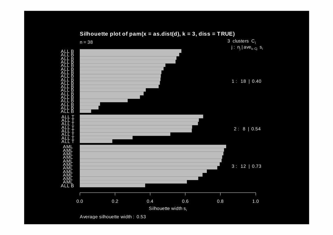
• the next plot is called a silhouette plot• each observation is represented by a

horizontal bar• the groups are slightly separated• the length of a bar is a measure of how

close the observation is to its assigned group (versus the others)

ALL BAML AML AML AML AML AML AML AML AML AML AML

ALL TALL TALL TALL TALL TALL TALL TALL TALL BALL BALL BALL BALL BALL BALL BALL BALL BALL BALL BALL BALL BALL BALL BALL BALL BALL B

Silhouette width si

0.0 0.2 0.4 0.6 0.8 1.0

Silhouette plot of pam(x = as.dist(d), k = 3, diss = TRUE)

Average silhouette width : 0.53

n = 38 3 clusters Cjj : nj | avei∈Cj si

1 : 18 | 0.40

2 : 8 | 0.54

3 : 12 | 0.73

Partitioning Methods: Comment

• Number of clusters, k:– If there are features that clearly distinguish

between the classes (e.g. cancer and healthy), the algorithm might use them to construct meaningful clusters.

– If the analysis has an exploratory character, one could repeat the clustering for several values of k.

Clustering Algorithm

• Partitioning: k-means, PAM• Hierarchical clustering • Model based: SOM

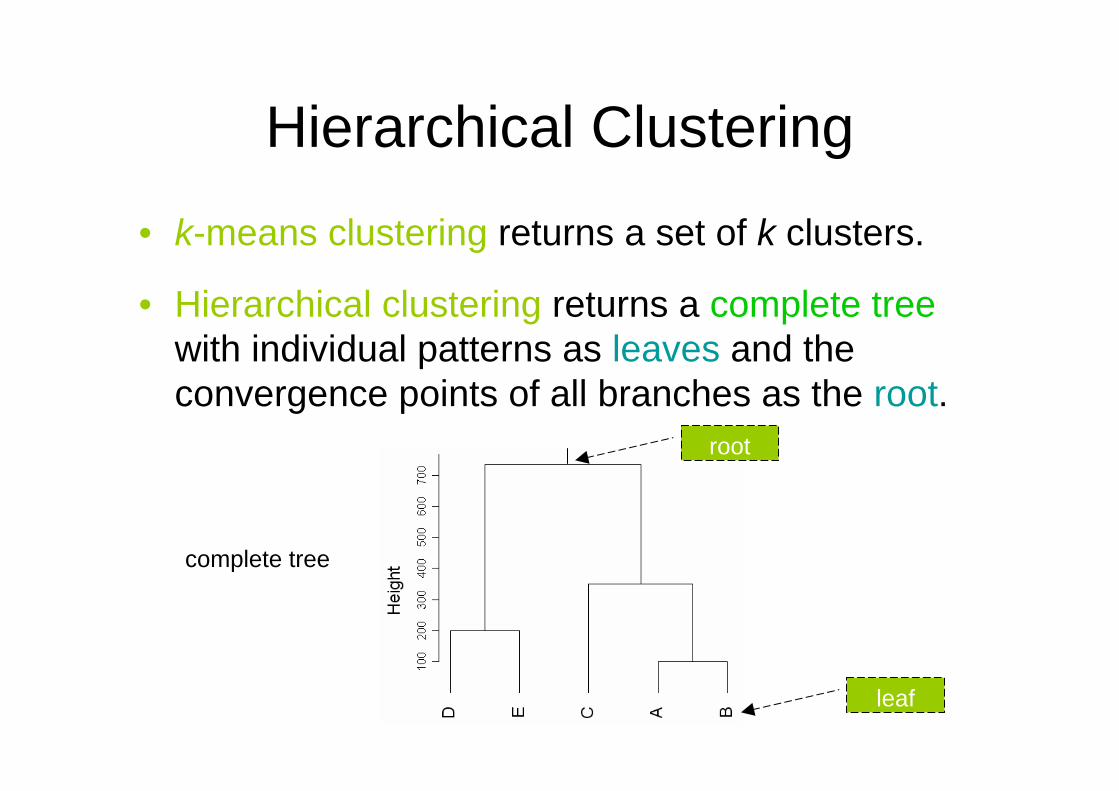
Hierarchical Clustering

• k-means clustering returns a set of k clusters.

• Hierarchical clustering returns a complete treewith individual patterns as leaves and the convergence points of all branches as the root.

Dis

tanc

ecomplete tree

leaf

root

Hierarchical Clustering

Step 1: Choose one distance measurement

Step 2: Construct the hierarchical tree:

– Bottom-up (agglomerative) method: n → 1; starting from the individual patterns and putting smaller clusters together to form bigger clusters.

– Top-down (divisive) method: 1 → n; starting at the root and splitting clusters into smaller ones by non-hierarchical algorithms (e.g., k-means with k = 2).

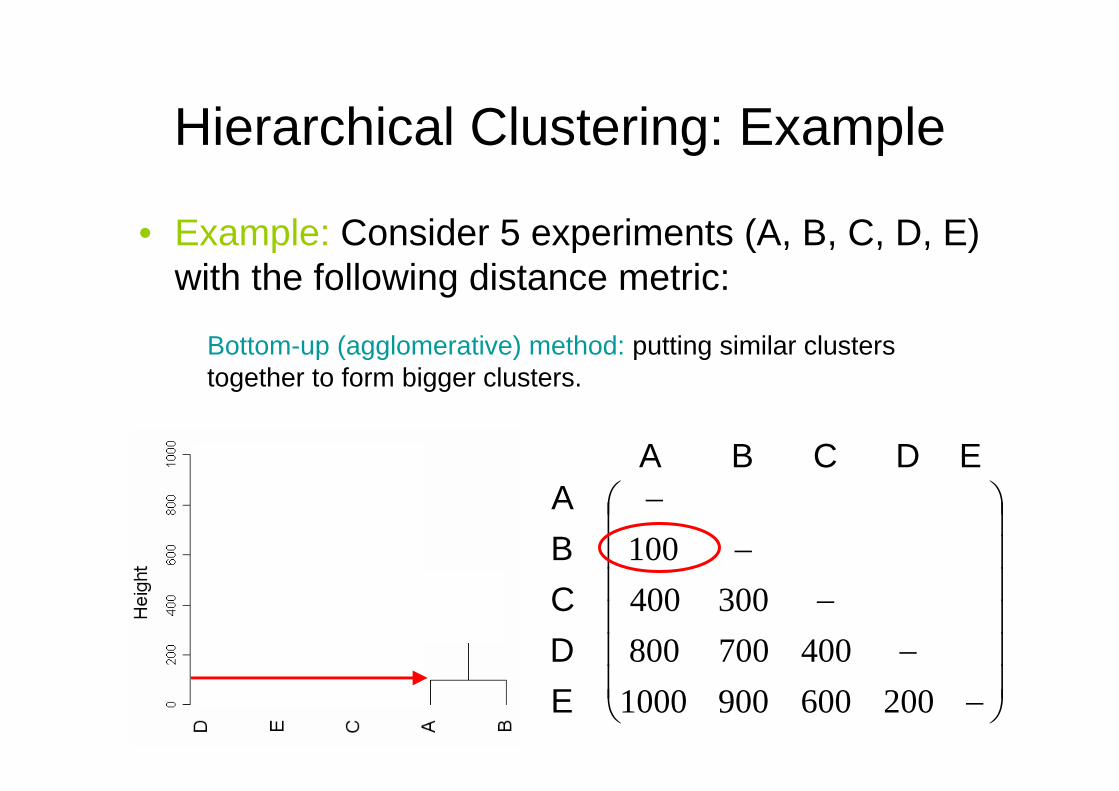
Hierarchical Clustering: Example

• Example: Consider 5 experiments (A, B, C, D, E) with the following distance metric:

⎟⎟⎟⎟⎟⎟

⎠

⎞

⎜⎜⎜⎜⎜⎜

⎝

⎛

−−

−−

−

2006009001000400700800

300400100

EDCBA

E D C B A

Bottom-up (agglomerative) method: putting similar clusters together to form bigger clusters.

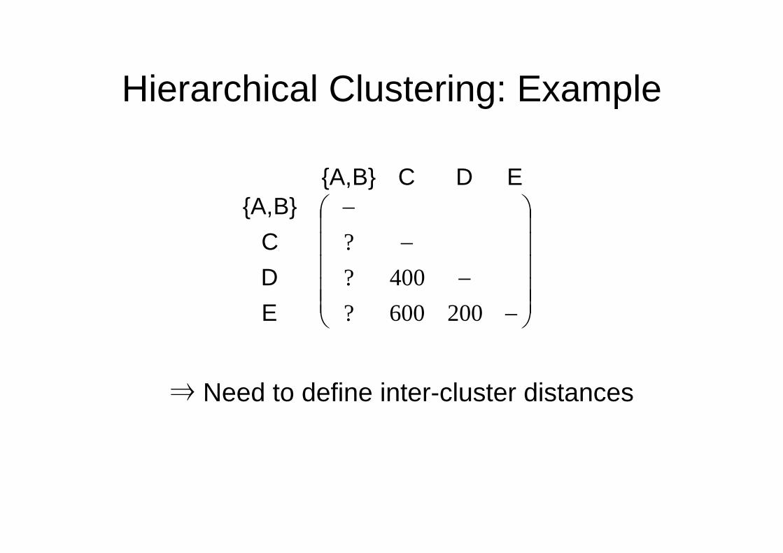
Hierarchical Clustering: Example

⎟⎟⎟⎟⎟

⎠

⎞

⎜⎜⎜⎜⎜

⎝

⎛

−−

−−

200600?400?

?

EDCB}{A,

E D CB}{A,

⇒ Need to define inter-cluster distances

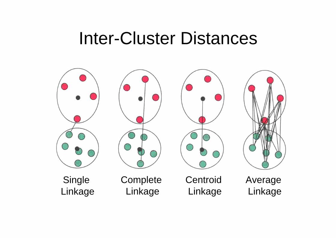
Inter-Cluster Distances

Single Linkage

Complete Linkage

CentroidLinkage

Average Linkage

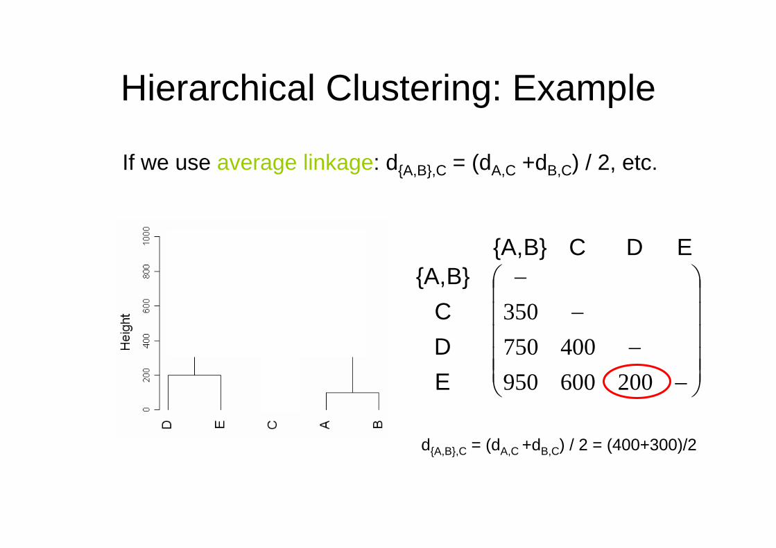
Hierarchical Clustering: Example

⎟⎟⎟⎟⎟

⎠

⎞

⎜⎜⎜⎜⎜

⎝

⎛

−−

−−

200600950400750

350

EDCB}{A,

E D CB}{A,

If we use average linkage: d{A,B},C = (dA,C +dB,C) / 2, etc.

d{A,B},C = (dA,C +dB,C) / 2 = (400+300)/2

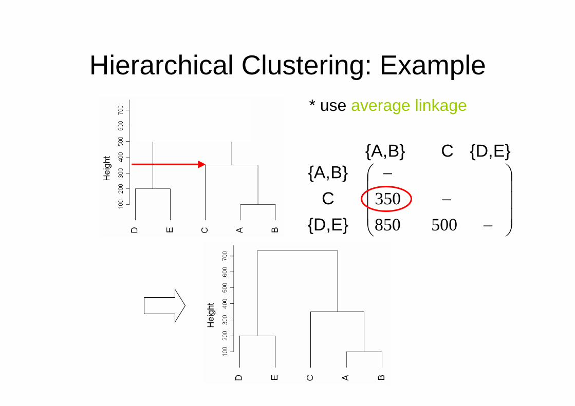
Hierarchical Clustering: Example

⎟⎟⎟

⎠

⎞

⎜⎜⎜

⎝

⎛

−−

−

E}{D,CB}{A,

E}{D,C B}{A,

500850350

* use average linkage

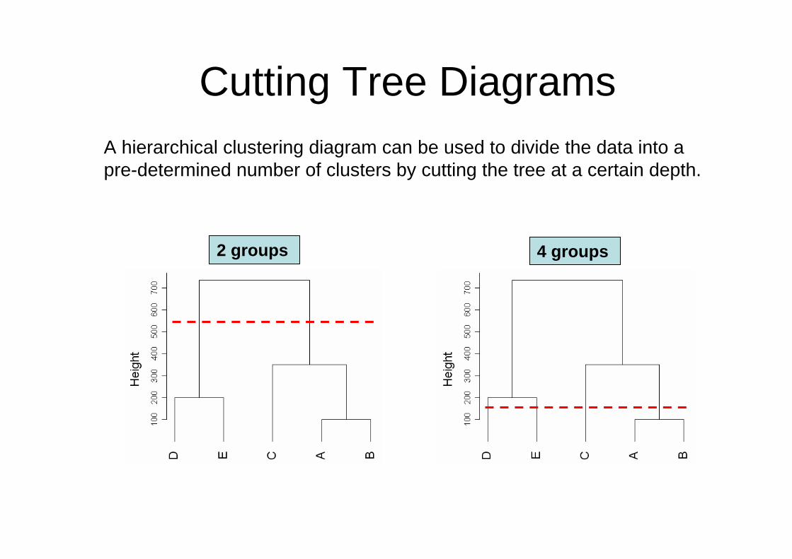
Cutting Tree Diagrams

2 groups 4 groups

A hierarchical clustering diagram can be used to divide the data into a pre-determined number of clusters by cutting the tree at a certain depth.

Properties of Hierarchical Clustering

• Different tree-constructing methods:– The same data and the same process obtain the

same results by running the same bottom-up method.

– The same data and the same process obtain twodifferent results by running the same top-down method.

• Different linkage type produce different results.

Hierarchical Clustering: Comments

• Objective of the research: To obtain a clustering that reflects the structure of the data. The dendrogram itself is almost never the answer to the research question.

• Various implementations of hierarchical clustering should not be judged simply by their speed; slower algorithms may be trying to do a better job pf extracting the data features.

• The order of the objects and clusters in the dendrogram may be misleading.

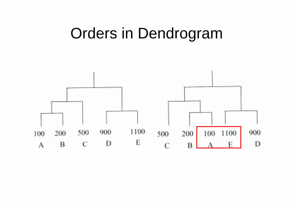
Orders in Dendrogram

Clustering Algorithm

• Partitioning: k-means, PAM• Hierarchical clustering • Model based: SOM

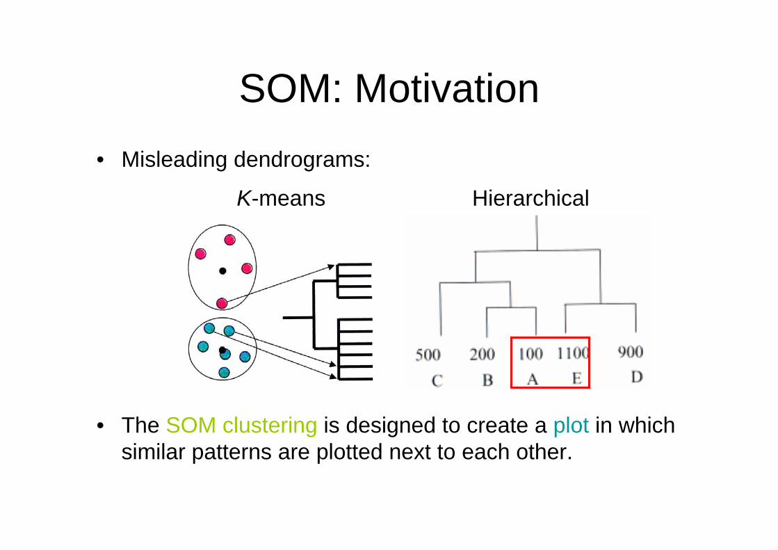
SOM: Motivation• Misleading dendrograms:

• The SOM clustering is designed to create a plot in which similar patterns are plotted next to each other.

K-means Hierarchical

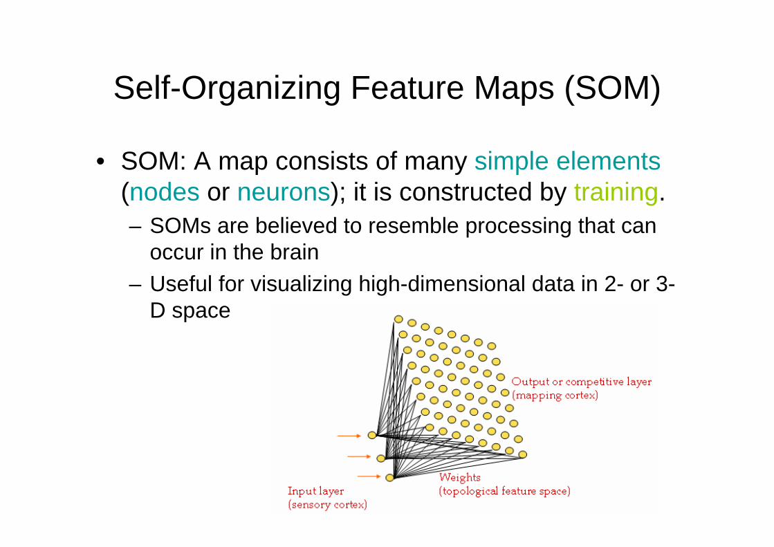
Self-Organizing Feature Maps (SOM)

• SOM: A map consists of many simple elements(nodes or neurons); it is constructed by training.– SOMs are believed to resemble processing that can

occur in the brain– Useful for visualizing high-dimensional data in 2- or 3-

D space

Self-Organizing Feature Maps (SOM)

• Clustering is performed by having several units competing for the current object

• The unit whose weight vector is closest to the current object wins

• The winner and its neighbors learn by having their weights adjusted

Self-Organizing Feature Maps (SOM)

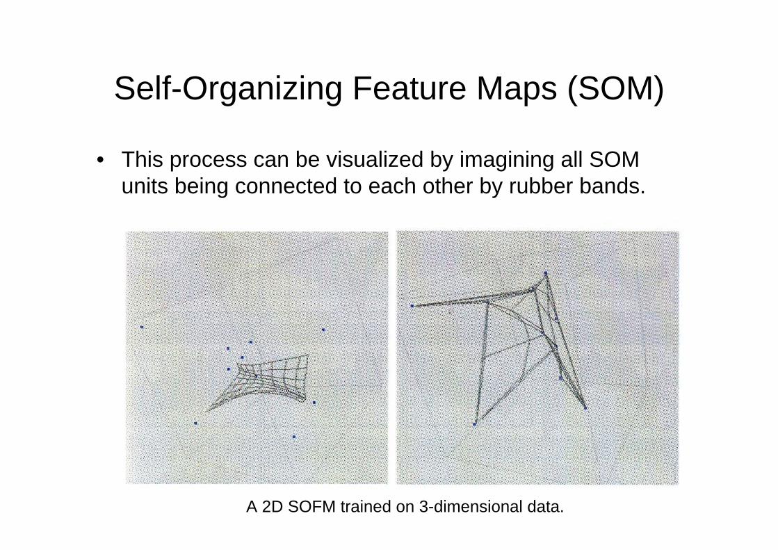
• This process can be visualized by imagining all SOM units being connected to each other by rubber bands.

A 2D SOFM trained on 3-dimensional data.

• paper:– Eisen 1998– Algorithmic Approaches to Clustering Gene

Expression Data http://citeseer.nj.nec.com/shamir01algorithmic.html

– Tibshirani, Hastie, Narasimhan and Chu (2002)http://www.pnas.org/cgi/reprint/99/10/6567

– Rousseeuw, P.J. (1987) Silhouettes: A graphical aid to the interpretation and validation of cluster analysis. J. Comput. Appl. Math., 20, 53–65