Measurement disturbance and conservation laws in quantum

Measurement disturbance and conservation laws in quantum mechanics

M. Hamed Mohammady,1, 2 Takayuki Miyadera,3 and Leon Loveridge4

1QuIC, Ecole Polytechnique de Bruxelles, CP 165/59,Universite Libre de Bruxelles, 1050 Brussels, Belgium

2RCQI, Institute of Physics, Slovak Academy of Sciences, Dubravska cesta 9, Bratislava 84511, Slovakia3Department of Nuclear Engineering, Kyoto University, Nishikyo-ku, Kyoto 615-8540, Japan

4Quantum Technology Group, Department of Science and Industry Systems,University of South-Eastern Norway, 3616 Kongsberg, Norway

We consider measurement disturbance for pairs of observables in the presence of a conservation law,providing conditions under which non-disturbance can be achieved. This is done by analysing the fixedpoint structure of the measurement channel. From here several extensions of the Wigner-Araki-Yanasetheorem are found.

1. INTRODUCTION

That measurements generally disturb quantum systems is one of the fundamental aspects of quantum mechanics. Thiseffect can be clearly seen when two observables are measured in succession, and the statistics of the second measurementdepends on whether the first measurement has taken place. The conditions under which measurement disturbance ariseshave now been well studied, and are intimately connected with whether the two observables are compatible [1].The disturbance caused by measurement depends both on the measured observable and on the details of the interactionbetween system and apparatus. If this interaction is constrained, there arise corresponding restrictions on the state changes.One example of this—and of central importance in this paper—is when the interaction is subject to a conservation law. Afamous such example is described by the Wigner-Araki-Yanase (WAY) theorem [2–4], in which a conservation law can beseen to either rule out measurements of a class of sharp observables, or impose conditions on the type of disturbance whichcan be achieved.Much previous work surrounding the WAY theorem (which has evolved over the years; its status and scope in 2011 isreported in [5]) has focused on the measurability question, or more generally, upon what cannot be done, or can be onlyapproximately done, given the conservation law. For instance, there are obstacles to the implementation of quantum logicgates [6–8]. The theorem continues to inspire research in a variety of directions (some recent examples are [9–15]), andconnections have been made to other fields of research; for instance in the resource theories of asymmetry [16] and coherence[17, 18], the theory of quantum reference frames [19], quantum clocks [20], and quantum thermodynamics [21–25].Despite this ongoing development, the full scope of the WAY theorem is not known; particularly, the role of disturbancehas not yet been carefully examined. Repeatability plays a central part in the original theorem and in this paper we take thebroader view that repeatability is a particular instance of non-disturbance, and we investigate WAY-type limitations in thissetting. We find that the presence of such limitations depends both on the observables considered and the details of themeasurement implementation, given as the structure of the set of fixed points of the measurement channel. The seconddirection we take comes from noting that measurements of unsharp observables in standard WAY-type scenarios is typicallylimited to their role as “approximators” of the desired sharp quantity. Though the WAY theorem rules out measurementsof sharp observables which do not commute with the conserved quantity, it does not rule out measurements of the unsharpapproximator, as is borne out in several early examples [5]. In the present paper, we analyse in more detail WAY-typemeasurement limitations for unsharp observables.In Sec. 2, the basic elements of the quantum theory of measurement are reviewed. Sec. 3 considers measurement disturbancein the presence of an additive conservation law—specifically the disturbance of an observable caused by the measurementof another. Independent of the conservation law, we provide a quantitative bound relating disturbance to the commutationbetween this pair of observables, which gives conditions under which zero disturbance can be achieved when the twoobservables do not commute. These conditions were previously reported in [26]. By contrast, in the presence of theconservation law, we obtain a bound which incorporates the additional feature that for non-disturbance the apparatus mustbe initialised in a state with a large spread in the conserved quantity, in the spirit of the original WAY theorem, but onlywhen the commutator of the unmeasured observable with the conserved quantity is not a fixed point of the measurementchannel. In Sec. 4 we consider the specific case where the measurement of an observable does not disturb itself, that is,when the measurement is first kind. In the case where this measurement is also repeatable, we provide an extension ofthe WAY theorem to observables that are not necessarily sharp. Finally, in Sec. 5 we consider how the structure of thefixed points of the measurement channel will impose restrictions on non-disturbance; if the measurement channel has afaithful fixed point, then the measurement is of the first kind only if the observable is commutative and commutes with

arX

iv:2

110.

1170

5v1

[qu

ant-

ph]

22

Oct

202

1

2

the conserved quantity. If the measurement channel does not contain any faithful fixed points, a more subtle restrictionapplies.

2. PRELIMINARIES

In this section we introduce notation and some basic elements of quantum theory that we use throughout the rest of thepaper. For further details, see, e.g., [27–30].

2.1. Operators on Hilbert space, operations, and channels

Let H be a complex separable Hilbert space, with L(H) ⊃ Ls(H) ⊃ Lp(H) the algebra of bounded (linear) operators, thereal vector space of self-adjoint operators, and the (cone of) positive operators on H, respectively. We shall denote by 1and O the identity and zero operators of L(H), respectively. We define by T (H) ⊆ L(H) the two-sided ideal of trace-classoperators on H. The (normal) state space of H is the space of positive, unit-trace operators S(H) ⊂ T (H), and a stateρ ∈ S(H) is called faithful if for all A ∈ L(H), tr[A∗Aρ] = 0 =⇒ A = O. If H is finite dimensional, a state is faithfulexactly when all its eigenvalues are strictly positive.Transformations of quantum systems are called operations, defined as completely positive (CP), trace non-increasinglinear maps Φ : T (H) → T (K). Among the operations are the channels, which preserve the trace. For any operationΦ : T (H) → T (K), there is an associated (Heisenberg picture) dual operation Φ∗ : L(K) → L(H), defined via the traceduality tr[Φ∗(A)T ] = tr[AΦ(T )] for all A ∈ L(K) and T ∈ T (H). Φ∗ is completely positive and sub-unital, and unitalexactly when Φ is trace-preserving.A unital CP map allows for the construction of an “operator-valued inner product”, which will be frequently used in thispaper.Lemma 2.1. Let Φ∗ : L(K) → L(H) be a unital CP map. Define an operator-valued sesquilinear mapping 〈〈·|·〉〉 :L(K)× L(K)→ L(H) by

〈〈A|B〉〉 := Φ∗(A∗B)− Φ∗(A∗)Φ∗(B),

to hold for all A,B ∈ L(K). Such a mapping satisfies (i) 〈〈A|B〉〉 = 〈〈B|A〉〉∗, (ii) 〈〈A|A〉〉 > O, and (iii) the Cauchy-Schwarz inequality

〈〈A|B〉〉〈〈B|A〉〉 6 ‖〈〈B|B〉〉‖〈〈A|A〉〉.

Property (i) is trivial, while (ii) follows from Kadison’s inequality [31]. The Cauchy-Schwarz inequality was proven byJanssens in Lemma 1 of Ref. [32], and we refer to Lemma 3 of Ref. [33] for an alternative proof. The above Lemma hasthe following useful consequence, which is known as the multiplication theorem:Corollary 2.1. Let Φ∗ : L(K)→ L(H) be a unital CP map, and suppose there is some B ∈ L(K) such that Φ∗(B∗B) =Φ∗(B∗)Φ∗(B). It follows that Φ∗(AB) = Φ∗(A)Φ∗(B) for all A ∈ L(K).

Proof. If Φ∗(B∗B) = Φ∗(B∗)Φ∗(B), then 〈〈B|B〉〉 = O, which implies that ‖〈〈B|B〉〉‖ = 0. Therefore, by Lemma 2.1 wehave for all A ∈ L(K) the following:

O 6 〈〈A∗|B〉〉〈〈A∗|B〉〉∗ = 〈〈A∗|B〉〉〈〈B|A∗〉〉 6 O.

This implies that 〈〈A∗|B〉〉 = Φ∗(AB)− Φ∗(A)Φ∗(B) = O.

For channels Φ : T (H)→ T (H), and their duals Φ∗ : L(H)→ L(H), we define the fixed-point sets as

F(Φ) := {T ∈ T (H) : Φ(T ) = T}, F(Φ∗) := {A ∈ L(H) : Φ∗(A) = A}.

Linearity of Φ∗ ensures that F(Φ∗) is closed under linear combinations, and because Φ∗ preserves the involution, F(Φ∗)∗ =F(Φ∗). In general, F(Φ∗) is not closed under multiplication. However, the following lemma provides a useful criterionunder which multiplicative closure is satisfied, in which case F(Φ∗) is a ∗-algebra. In fact, as we shall soon see, it is a vonNeumann algebra.Lemma 2.2 (Lindblad). Assume that F(Φ) contains a faithful state. Then F(Φ∗) is a von Neumann algebra.

3

Proof. Suppose B ∈ F(Φ∗). Let us define the operator Φ∗(B∗B)− Φ∗(B∗)Φ∗(B) = Φ∗(B∗B)−B∗B, which is positivedue to Kadison’s inequality. Let F(Φ) contain a faithful state ω. Then we have

tr[ω(Φ∗(B∗B)−B∗B)] = tr[ω(B∗B −B∗B)] = 0,

which implies that Φ∗(B∗B) = B∗B. Corollary 2.1 therefore implies that for all A ∈ L(H),

Φ∗(AB) = Φ∗(A)B.

Therefore, if A ∈ F(Φ∗), then Φ∗(AB) = AB, and so F(Φ∗) is closed under multiplication and therefore a ∗-algebra.Finally, if F(Φ∗) is an algebra, then F(Φ∗) = {Ki,K

∗i }′ := {A ∈ L(H) : [Ki, A] = [K∗i , A] = O∀i}, with {Ki} any

Kraus representation of Φ [34], making F(Φ∗) a von Neumann algebra (as the commutant of a self-adjoint subset of L(H))[35].

2.2. Observables, instruments, and measurement schemes

In general, the state changes, or disturbance caused by measurements are captured by the notion of an instrument,or operation valued measure [36–40]. In this section, we provide some background on instruments, observables andmeasurement schemes, as part of the quantum theory of measurement.Given a quantum system S, with Hilbert space HS , an observable of S is represented by a normalised positive operatorvalued measure (POVM) E : Σ→ Lp(HS), where Σ is a σ−algebra of subsets of some value space X , representing possibleoutcomes of a measurement of E. E(X) is positive for any X ∈ Σ, sigma-additive on disjoint elements of Σ, and E(X )is the identity operator on HS . Discrete observables are those for which X = {x1, x2, . . . } is countable. In such a case Ecan be identified with the set {E(x) ≡ E({x}) ∈ Lp(HS) : x ∈ X} ≡ E. If it is not stated otherwise, observables will beassumed to be discrete. Combined with states, observables give rise to the probabilities

pEρ(x) := tr[E(x)ρ],

holding for all ρ ∈ S(HS) and all x ∈ X , interpreted as the probability of observing outcome x when the observable E ismeasured in the state ρ.If E is a POVM acting in HS , the commutant of E is denoted by E′ := {A ∈ L(HS) : [E(x), A] = O∀x ∈ X}. SinceE = E∗ is a self-adjoint set, E′ is a von Neumann algebra, and E′′ ≡ (E′)′ is the smallest von Neumann algebra containing E(i.e., it is the von Neumann algebra generated by E). For any A ∈ L(HS) for which A ∈ E′, we write [E, A] = O. Similarly,for any observable F := {F(y) : y ∈ Y} such that F ⊂ E′, we shall write [E,F] = O. Among the observables are thosewhich are commutative, meaning that E ⊂ E′ (that is, all the effects E(x) mutually commute). Among the commutativeobservables are the sharp observables, which satisfy the additional condition that for all x, y ∈ X , E(x)E(y) = δx,yE(x),i.e., E(x) are projection operators. These observables correspond to self-adjoint operators through the spectral theorem.Observables which are not sharp will be called unsharp, and we may quantify the unsharpness of the effects of E by theoperator norm as ‖E(x)− E(x)2‖, which vanishes exactly when E(x) = E(x)2.

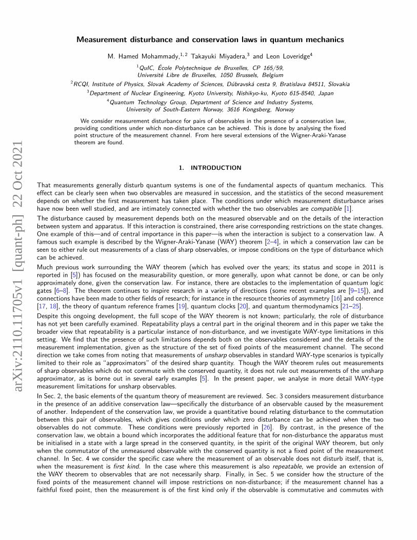
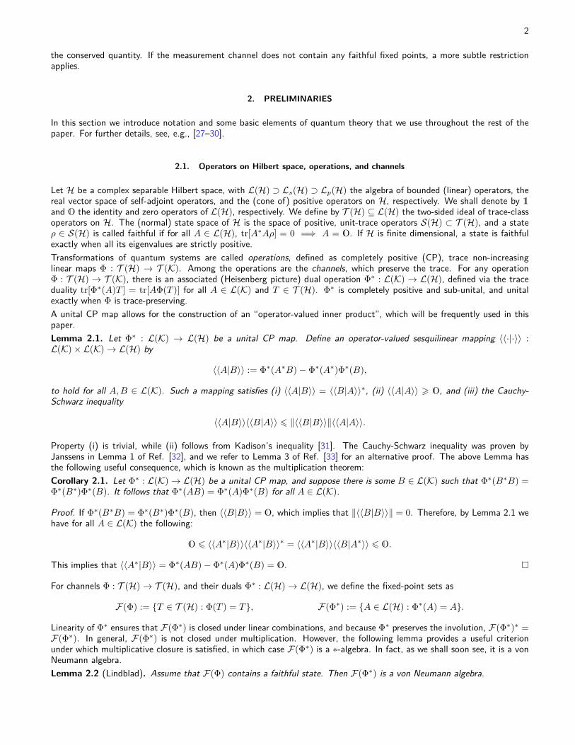
FIG. 1: An instrument measures an observable E of the system S, and also transforms the system conditional on registering a given out-come. The system, initially prepared in an arbitrary state ρ, enters the instrument which then registers outcome x with probability pE

ρ(x) :=tr[E(x)ρ] = tr[Ix(ρ)]. Subsequently, the instrument transforms the system to the (non-normalised) state Ix(ρ).Though the state-observable pairings describe the totality of the measurement statistics, this is not sufficient for determiningother interesting properties of a measurement, for instance the form of the associated state change. To this end, we makeuse of the notion of instrument, or operation valued measure [36]. A discrete instrument is a collection of operationsI := {Ix ≡ I{x} : x ∈ X}, where Ix : T (HS) → T (HS), such that

∑x∈X tr[Ix(T )] = tr[T ] for all T ∈ T (HS). IX ,

defined by IX (T ) =∑x∈X Ix(T ), is the channel induced by the instrument I. Each instrument is associated with a unique

observable E via I∗x(1S) = E(x), which implies that pEρ(x) = tr[E(x)ρ] = tr[Ix(ρ)]. We refer to I as an E-compatible

instrument, or an E-instrument for short. Ix(ρ) is interpreted as the non-normalised state after a measurement of E has

4

taken place and the outcome x has been registered, and IX (ρ) is the normalised state when the system has been subjectto a non-selective measurement by I. A schematic representation of an instrument is given in Fig. 1.We note that for every discrete observable E, there are infinitely many E-compatible instruments; every E-instrument I canbe constructed as the set of operations {Φx ◦ ILx : x ∈ X} [38, 40], where Φx : T (HS) → T (HS) are arbitrary channels,and IL is the Luders instrument for E [41], defined as

ILx (T ) :=√

E(x)T√

E(x), ILx∗(A) :=

√E(x)A

√E(x), (1)

to hold for all x ∈ X , T ∈ T (HS), and A ∈ L(HS).

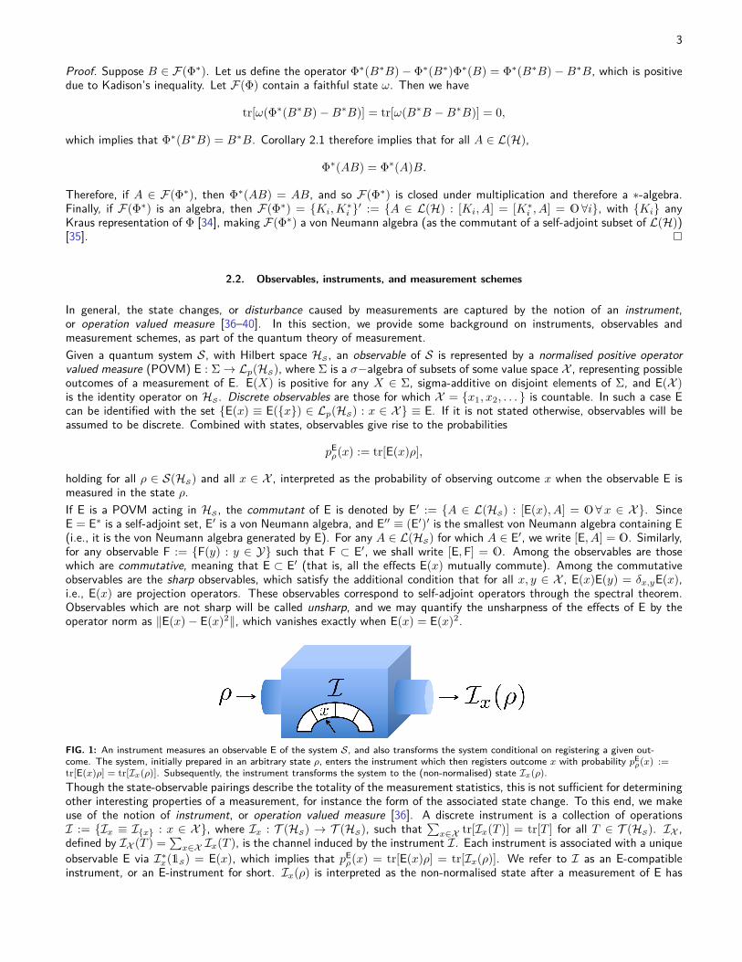
FIG. 2: An E-instrument I is implemented on the system S via a measurement scheme. The system, initially prepared in an arbitrary state ρ,and a measurement apparatus A, prepared in a fixed state ξ, undergo a joint unitary evolution U . Subsequently, a sharp pointer observable Zof the apparatus is measured. With probability pE

ρ(x) := tr[E(x)ρ] = tr[Ix(ρ)] the apparatus registers outcome x, thereby transforming thesystem to the non-normalised state Ix(ρ).An even more comprehensive description of the measurement process involves the modelling of a measuring apparatus Aand a specification of how it couples to the system under investigation. Every E-instrument I on HS admits a measurementscheme M := (HA, ξ, U,Z) [42] where: HA is the Hilbert space for the measurement apparatus A and ξ ∈ S(HA) is astate of the apparatus; U : HS ⊗HA → HS ⊗HA is a unitary coupling on HS ⊗HA which serves to correlate system andapparatus; and Z := {Z(x) : x ∈ X} is a (sharp) “pointer” observable of the apparatus, which we choose to have the samevalue space X as the system observable E . The operations of the instrument can be written

Ix(T ) = trA[(1S ⊗ Z(x))U(T ⊗ ξ)U∗] (2)

for all T ∈ T (HS) and x ∈ X , where trA : T (HS ⊗HA) → T (HS) is the partial trace channel over the apparatus. Theinstrument channel may thus be written as IX (T ) = trA[U(T ⊗ ξ)U∗]. A schematic representation of a measurementscheme is given in Fig. 2.Let us now introduce the unital, completely positive normal conditional expectation Γξ : L(HS ⊗ HA) → L(HS). Γξ,called a restriction map for ξ, is defined as the dual of the isometric embedding (or the preparation map) T 7→ T ⊗ ξ, andsatisfies tr[Γξ(B)T ] = tr[B(T ⊗ ξ)] for all B ∈ L(HS ⊗HA) and T ∈ T (HS). We may use the restriction map to definethe (unital, completely positive) map ΓUξ : L(HS ⊗HA)→ L(HS) as

ΓUξ (B) := Γξ(U∗BU), (3)

to hold for all B ∈ L(HS ⊗HA). Using Eq. (3), we may express the dual of the operations defined in Eq. (2) as

I∗x(A) = ΓUξ (A⊗ Z(x)), (4)

for all A ∈ L(HS) and x ∈ X . Therefore, we may write E(x) = I∗x(1S) = ΓUξ (1S⊗Z(x)), and I∗X (A) = ΓUξ (A⊗1A).

3. QUANTIFYING MEASUREMENT DISTURBANCE IN THE PRESENCE OF ADDITIVE CONSERVATION LAWS

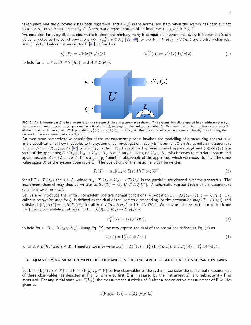
Let E := {E(x) : x ∈ X} and F := {F(y) : y ∈ Y} be two observables of the system. Consider the sequential measurementof these observables, as depicted in Fig. 3, where at first E is measured by the instrument I, and subsequently F ismeasured. For any initial state ρ ∈ S(HS), the measurement statistics of F after a non-selective measurement of E will begiven as

tr[F(y)IX (ρ)] ≡ tr[I∗X (F(y))ρ].

5

FIG. 3: In a sequential measurement, an observable E is measured by an instrument I, and subsequently a second observable F is measured.I does not disturb F if for all input states ρ, the statistics of F does not depend on whether an E-measurement took place or not. I does notdisturb F precisely when F is contained in the fixed-point set of the E-channel I∗X .

That is, the measurement statistics of F will be determined by the disturbed effects I∗X (F(y)). We may define the“difference” between the disturbed and non-disturbed effects of F by the operators

δ(y) := I∗X (F(y))− F(y). (5)

The disturbance of F(y) by I may therefore be quantified as ‖δ(y)‖, which has the operational meaning as (the least upperbound of) the largest possible discrepancy between the probability distributions arising from the disturbed and non-disturbedeffects:

‖δ(y)‖ = supρ∈S(HS )

∣∣∣∣tr[I∗X (F(y))ρ]− tr[F(y)ρ]∣∣∣∣.

A global quantification of the disturbance of F can then be defined as the largest disturbance of one of the effects,

δ := maxy∈Y‖δ(y)‖,

and F is non-disturbed by I exactly when δ = 0, which implies that

I∗X (F(y)) = F(y) ∀ y ∈ Y. (6)

In other words, I does not disturb F exactly when each F(y) is a fixed point of the E-channel I∗X , i.e., F ⊂ F(I∗X ). In sucha case, for any initial state ρ the measurement statistics of F will not depend on whether or not an E-measurement tookplace.Non-disturbance of F by the E-instrument I implies that E and F are compatible (or jointly measurable) [1], i.e., thereexists a joint observable G := {G(x, y) : (x, y) ∈ X × Y} such that∑

y∈YG(x, y) = E(x),

∑x∈X

G(x, y) = F(y) ∀x ∈ X , y ∈ Y. (7)

If F ⊂ F(I∗X ), we may choose G as G(x, y) = I∗x(F(y)), which satisfies Eq. (7). We may therefore conclude that for twoincompatible observables E and F, no E-instrument I exists that satisfies F ⊂ F(I∗X ). Note that while non-disturbancerequires compatibility, compatibility does not guarantee non-disturbance. For instance, while any observable is compatiblewith itself, for every informationally complete observable the fixed point set of its compatible channel becomes trivial.Indeed, the size of the fixed-point set of an E-channel is strongly relevant to the amount of information given by E as shownin Ref. [43]. Furthermore, as shown in Ref. [26], there exist pairs of compatible observables E and F where E admits aninstrument that does not disturb F, but all possible F-instruments necessarily disturb E. This further demonstrates thatunlike compatibility, non-disturbance is not symmetric.As shown in Ref. [44], the pair of observables E and F are compatible only if

‖[E(x),F(y)]‖ 6 2‖E(x)− E(x)2‖1/2‖F(y)− F(y)2‖1/2 ∀x ∈ X , y ∈ Y. (8)

Commutativity is a sufficient condition for compatibility; if E commutes with F, then there is always a joint observable Gwith effects G(x, y) = E(x)F(y), which are positive since they can be written as G(x, y) = (

√E(x)

√F(y))∗(

√E(x)

√F(y)).

On the other hand, if either E or F is sharp, in which case the upper bound of Eq. (8) vanishes, then commutativity is anecessary condition for compatibility [45]. For two non-commuting observables to be compatible, therefore, their effectsmust be sufficiently unsharp.We now provide a bound for the commutation between the effects of E and F in terms of the disturbance of F by I.

6

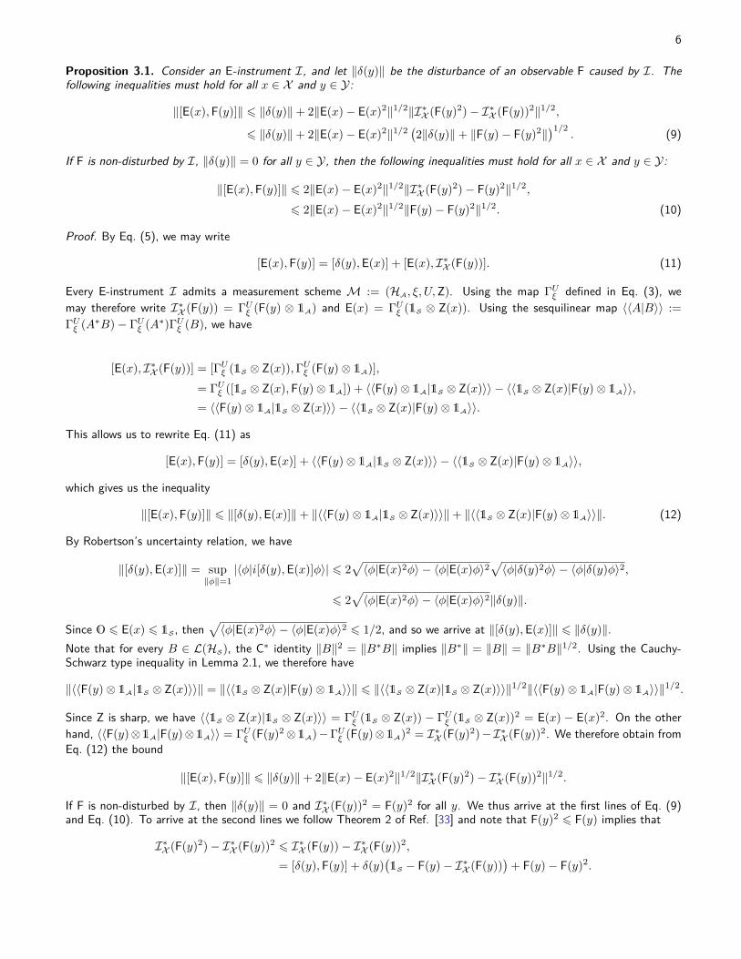
Proposition 3.1. Consider an E-instrument I, and let ‖δ(y)‖ be the disturbance of an observable F caused by I. Thefollowing inequalities must hold for all x ∈ X and y ∈ Y:

‖[E(x),F(y)]‖ 6 ‖δ(y)‖+ 2‖E(x)− E(x)2‖1/2‖I∗X (F(y)2)− I∗X (F(y))2‖1/2,

6 ‖δ(y)‖+ 2‖E(x)− E(x)2‖1/2 (2‖δ(y)‖+ ‖F(y)− F(y)2‖)1/2

. (9)

If F is non-disturbed by I, ‖δ(y)‖ = 0 for all y ∈ Y, then the following inequalities must hold for all x ∈ X and y ∈ Y:

‖[E(x),F(y)]‖ 6 2‖E(x)− E(x)2‖1/2‖I∗X (F(y)2)− F(y)2‖1/2,

6 2‖E(x)− E(x)2‖1/2‖F(y)− F(y)2‖1/2. (10)

Proof. By Eq. (5), we may write

[E(x),F(y)] = [δ(y),E(x)] + [E(x), I∗X (F(y))]. (11)

Every E-instrument I admits a measurement scheme M := (HA, ξ, U,Z). Using the map ΓUξ defined in Eq. (3), wemay therefore write I∗X (F(y)) = ΓUξ (F(y) ⊗ 1A) and E(x) = ΓUξ (1S ⊗ Z(x)). Using the sesquilinear map 〈〈A|B〉〉 :=ΓUξ (A∗B)− ΓUξ (A∗)ΓUξ (B), we have

[E(x), I∗X (F(y))] = [ΓUξ (1S ⊗ Z(x)),ΓUξ (F(y)⊗ 1A)],= ΓUξ ([1S ⊗ Z(x),F(y)⊗ 1A]) + 〈〈F(y)⊗ 1A|1S ⊗ Z(x)〉〉 − 〈〈1S ⊗ Z(x)|F(y)⊗ 1A〉〉,= 〈〈F(y)⊗ 1A|1S ⊗ Z(x)〉〉 − 〈〈1S ⊗ Z(x)|F(y)⊗ 1A〉〉.

This allows us to rewrite Eq. (11) as

[E(x),F(y)] = [δ(y),E(x)] + 〈〈F(y)⊗ 1A|1S ⊗ Z(x)〉〉 − 〈〈1S ⊗ Z(x)|F(y)⊗ 1A〉〉,

which gives us the inequality

‖[E(x),F(y)]‖ 6 ‖[δ(y),E(x)]‖+ ‖〈〈F(y)⊗ 1A|1S ⊗ Z(x)〉〉‖+ ‖〈〈1S ⊗ Z(x)|F(y)⊗ 1A〉〉‖. (12)

By Robertson’s uncertainty relation, we have

‖[δ(y),E(x)]‖ = sup‖φ‖=1

|〈φ|i[δ(y),E(x)]φ〉| 6 2√〈φ|E(x)2φ〉 − 〈φ|E(x)φ〉2

√〈φ|δ(y)2φ〉 − 〈φ|δ(y)φ〉2,

6 2√〈φ|E(x)2φ〉 − 〈φ|E(x)φ〉2‖δ(y)‖.

Since O 6 E(x) 6 1S , then√〈φ|E(x)2φ〉 − 〈φ|E(x)φ〉2 6 1/2, and so we arrive at ‖[δ(y),E(x)]‖ 6 ‖δ(y)‖.

Note that for every B ∈ L(HS), the C∗ identity ‖B‖2 = ‖B∗B‖ implies ‖B∗‖ = ‖B‖ = ‖B∗B‖1/2. Using the Cauchy-Schwarz type inequality in Lemma 2.1, we therefore have

‖〈〈F(y)⊗ 1A|1S ⊗ Z(x)〉〉‖ = ‖〈〈1S ⊗ Z(x)|F(y)⊗ 1A〉〉‖ 6 ‖〈〈1S ⊗ Z(x)|1S ⊗ Z(x)〉〉‖1/2‖〈〈F(y)⊗ 1A|F(y)⊗ 1A〉〉‖1/2.

Since Z is sharp, we have 〈〈1S ⊗ Z(x)|1S ⊗ Z(x)〉〉 = ΓUξ (1S ⊗ Z(x)) − ΓUξ (1S ⊗ Z(x))2 = E(x) − E(x)2. On the otherhand, 〈〈F(y)⊗1A|F(y)⊗1A〉〉 = ΓUξ (F(y)2⊗1A)−ΓUξ (F(y)⊗1A)2 = I∗X (F(y)2)−I∗X (F(y))2. We therefore obtain fromEq. (12) the bound

‖[E(x),F(y)]‖ 6 ‖δ(y)‖+ 2‖E(x)− E(x)2‖1/2‖I∗X (F(y)2)− I∗X (F(y))2‖1/2.

If F is non-disturbed by I, then ‖δ(y)‖ = 0 and I∗X (F(y))2 = F(y)2 for all y. We thus arrive at the first lines of Eq. (9)and Eq. (10). To arrive at the second lines we follow Theorem 2 of Ref. [33] and note that F(y)2 6 F(y) implies that

I∗X (F(y)2)− I∗X (F(y))2 6 I∗X (F(y))− I∗X (F(y))2,

= [δ(y),F(y)] + δ(y)(1S − F(y)− I∗X (F(y))

)+ F(y)− F(y)2.

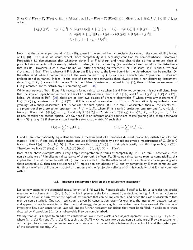
7

Since O 6 F(y) + I∗X (F(y)) 6 21S , it follows that ‖1S − F(y) − I∗X (F(y))‖ 6 1. Given that ‖[δ(y),F(y)]‖ 6 ‖δ(y)‖, weobtain

‖I∗X (F(y)2)− I∗X (F(y))2‖ 6 ‖[δ(y),F(y)]‖+ ‖δ(y)(1S − F(y)− I∗X (F(y))

)‖+ ‖F(y)− F(y)2‖,

6 ‖δ(y)‖+ ‖δ(y)‖‖1S − F(y)− I∗X (F(y))‖+ ‖F(y)− F(y)2‖,6 2‖δ(y)‖+ ‖F(y)− F(y)2‖.

Note that the larger upper bound of Eq. (10), given in the second line, is precisely the same as the compatibility boundof Eq. (8). This is as we would expect, since compatibility is a necessary condition for non-disturbance. Moreover,Proposition 3.1 demonstrates that whenever either E or F is sharp, and these observables do not commute, then allpossible E-instruments will necessarily disturb F. Indeed, in such a case Eq. (9) provides a lower bound for the disturbancethat results. However, such a lower bound will differ depending on whether E or F is sharp; if E is sharp, we haveδ > maxx,y ‖[E(x),F(y)]‖, whereas if F is sharp but E is unsharp, the lower bound for the disturbance may be smaller. Onthe other hand, when E commutes with F the lower bound of Eq. (10) vanishes, in which case Proposition 3.1 does notprohibit non-disturbance. Indeed, in the case of commuting observables there always exists a non-disturbing instrument;since E′ ⊂ F(ILX

∗) always holds, where IL is the Luders E-instrument defined in Eq. (1), then a Luders measurement ofE is guaranteed not to disturb any F commuting with E [46].While unsharpness of both E and F is necessary for non-disturbance when E and F do not commute, it is not sufficient. Notethat the smaller upper bound in the first line of Eq. (10) vanishes if both F ⊂ F(I∗X ) and F2 := {F(y)2 : y ∈ Y} ⊂ F(I∗X )holds. As shown in Ref. [26], there are at least two classes of unsharp observables F where given any instrument I,F ⊂ F(I∗X ) guarantees that F2 ⊂ F(I∗X ): if F is a rank-1 observable, or if F is an “informationally equivalent coarse-graining” of a sharp observable. Let us consider the first option. If F is a rank-1 observable, then all the effects of Fare proportional to a projection operator, i.e., F(y) = λyPy, where Py is a rank-1 projection operator and λy ∈ (0, 1]. Ittrivially follows that I∗X (F(y)) = F(y) if and only if I∗X (Py) = Py. As such, I∗X (F(y)2) = λ2

yI∗X (Py) = λ2yPy = F(y)2. Let

us now consider the second option. We say that F is an informationally equivalent coarse-graining of a sharp observableG := {G(z) : z ∈ Z} if there exists an invertible stochastic matrix M such that

F(y) =∑z

My,zG(z), G(z) =∑y

M−1z,yF(y).

F and G are informationally equivalent because a measurement of F produces different probability distributions for twostates ρ1 and ρ2 if and only if these states produce different probability distributions given a measurement of G. Since Gis sharp, then F(y)2 =

∑zM

2y,zG(z). Now assume that F ⊂ F(I∗X ). It is simple to verify that this implies G ⊂ F(I∗X ).

Therefore, we have I∗X (F(y)2) =∑zM

2y,zI∗X (G(z)) =

∑zM

2y,zG(z) = F(y)2.

Both of the above examples offer a very simple interpretation in terms of compatibility. If F is a rank-1 observable, thennon-disturbance of F implies non-disturbance of sharp rank-1 effects Py. Since non-disturbance requires compatibility, thisimplies that E must commute with all Py, and hence with F. On the other hand, if F is a classical coarse-graining of asharp observable G, then non-disturbance of F implies non-disturbance of G, and by compatibility E must commute withG. Since the effects of F are constructed as a mixture of the (projective) effects of G, this concludes that E must commutewith F.

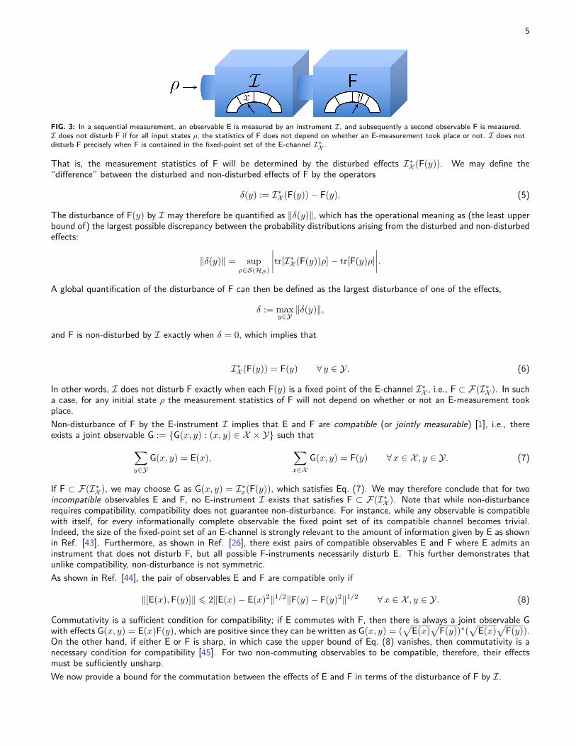
3.1. Imposing conservation laws on the measurement interaction

Let us now examine the sequential measurement of E followed by F more closely. Specifically, let us consider the precisemeasurement scheme M := (HA, ξ, U,Z) which implements the E-instrument I, as depicted in Fig. 4. Any restrictions weimpose onM will in turn restrict the types of instruments that can be implemented, and hence the class of observables thatmay be non-disturbed. One such restriction is given by conservation laws—for example, the interaction between systemand apparatus may be restricted so that the total energy, charge, or angular momentum must be conserved. We shall nowinvestigate how such conservation laws will impose further necessary conditions that must be fulfilled, in addition to thosedictated by Proposition 3.1, for an observable F to be non-disturbed.We say that M is subject to an additive conservation law if there exists a self-adjoint operator N = NS ⊗ 1A + 1S ⊗NA,where NS ∈ Ls(HS) and NA ∈ Ls(HA), such that [U,N ] = O. As we show below, non-disturbance of F by a measurementof E subject to a conservation law imposes constraints on the commutation between the effects of F and the system partof the conserved quantity, NS .

8

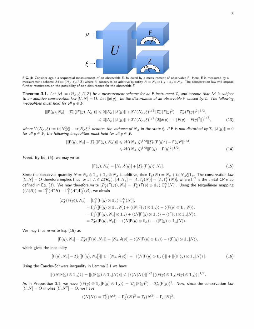
FIG. 4: Consider again a sequential measurement of an observable E, followed by a measurement of observable F. Here, E is measured by ameasurement scheme M := (HA, ξ, U,Z) where U conserves an additive quantity N = NS ⊗1A +1S ⊗NA. The conservation law will imposefurther restrictions on the possibility of non-disturbance for the observable F

Theorem 3.1. Let M := (HA, ξ, U,Z) be a measurement scheme for an E-instrument I, and assume that M is subjectto an additive conservation law [U,N ] = O. Let ‖δ(y)‖ be the disturbance of an observable F caused by I. The followinginequalities must hold for all y ∈ Y:

‖[F(y), NS ]− I∗X ([F(y), NS ])‖ 6 2‖NS‖‖δ(y)‖+ 2V (NA, ξ)1/2‖I∗X (F(y)2)− I∗X (F(y))2‖1/2,

6 2‖NS‖‖δ(y)‖+ 2V (NA, ξ)1/2 (2‖δ(y)‖+ ‖F(y)− F(y)2‖)1/2

, (13)

where V (NA, ξ) := tr[N2Aξ]− tr[NAξ]2 denotes the variance of NA in the state ξ. If F is non-disturbed by I, ‖δ(y)‖ = 0

for all y ∈ Y, the following inequalities must hold for all y ∈ Y:

‖[F(y), NS ]− I∗X ([F(y), NS ])‖ 6 2V (NA, ξ)1/2‖I∗X (F(y)2)− F(y)2‖1/2,

6 2V (NA, ξ)1/2‖F(y)− F(y)2‖1/2. (14)

Proof. By Eq. (5), we may write

[F(y), NS ] = [NS , δ(y)] + [I∗X (F(y)), NS ]. (15)

Since the conserved quantity N = NS ⊗ 1A + 1S ⊗NA is additive, then Γξ(N) = NS + tr[NAξ]1S . The conservation law[U,N ] = O therefore implies that for all A ∈ L(HS), [A,NS ] = [A,Γξ(N)] = [A,ΓUξ (N)], where ΓUξ is the unital CP mapdefined in Eq. (3). We may therefore write [I∗X (F(y)), NS ] = [ΓUξ (F(y) ⊗ 1A),ΓUξ (N)]. Using the sesquilinear mapping〈〈A|B〉〉 := ΓUξ (A∗B)− ΓUξ (A∗)ΓUξ (B), we obtain

[I∗X (F(y)), NS ] = [ΓUξ (F(y)⊗ 1A),ΓUξ (N)],= ΓUξ ([F(y)⊗ 1A, N ]) + 〈〈N |F(y)⊗ 1A〉〉 − 〈〈F(y)⊗ 1A|N〉〉,= ΓUξ ([F(y), NS ]⊗ 1A) + 〈〈N |F(y)⊗ 1A〉〉 − 〈〈F(y)⊗ 1A|N〉〉,= I∗X ([F(y), NS ]) + 〈〈N |F(y)⊗ 1A〉〉 − 〈〈F(y)⊗ 1A|N〉〉.

We may thus re-write Eq. (15) as

[F(y), NS ] = I∗X ([F(y), NS ]) + [NS , δ(y)] + 〈〈N |F(y)⊗ 1A〉〉 − 〈〈F(y)⊗ 1A|N〉〉,

which gives the inequality

‖[F(y), NS ]− I∗X ([F(y), NS ])‖ 6 ‖[NS , δ(y)]‖+ ‖〈〈N |F(y)⊗ 1A〉〉‖+ ‖〈〈F(y)⊗ 1A|N〉〉‖. (16)

Using the Cauchy-Schwarz inequality in Lemma 2.1 we have

‖〈〈N |F(y)⊗ 1A〉〉‖ = ‖〈〈F(y)⊗ 1A|N〉〉‖ 6 ‖〈〈N |N〉〉‖1/2‖〈〈F(y)⊗ 1A|F(y)⊗ 1A〉〉‖1/2.

As in Proposition 3.1, we have 〈〈F(y) ⊗ 1A|F(y) ⊗ 1A〉〉 = I∗X (F(y)2) − I∗X (F(y))2. Now, since the conservation law[U,N ] = O implies [U,N2] = O, we have

〈〈N |N〉〉 = ΓUξ (N2)− ΓUξ (N)2 = Γξ(N2)− Γξ(N)2.

9

Note that N2 = N2S ⊗ 1A + 2NS ⊗NA + 1S ⊗N2

A. Therefore, we have

Γξ(N2) = N2S + 2tr[NAξ]NS + tr[N2

Aξ]1S ,

Γξ(N)2 = N2S + 2tr[NAξ]NS + tr[NAξ]21S ,

which gives

〈〈N |N〉〉 = tr[N2Aξ]1S − tr[NAξ]21S =: V (NA, ξ)1S . (17)

Noting that ‖[NS , δ(y)]‖ 6 2‖NS‖‖δ(y)‖, we thus obtain from Eq. (16) the inequality

‖[F(y), NS ]− I∗X ([F(y), NS ])‖ 6 2‖NS‖‖δ(y)‖+ 2V (NA, ξ)1/2‖I∗X (F(y)2)− I∗X (F(y))2‖1/2.

If F is non-disturbed by I, then ‖δ(y)‖ = 0 and I∗X (F(y))2 = F(y)2 for all y. We thus arrive at the first lines of Eq. (13)and Eq. (14). To arrive at the second lines we note that, as shown in Theorem 2 of Ref. [33] and recapitulated inProposition 3.1, it holds that ‖I∗X (F(y)2)− I∗X (F(y))2‖ 6 2‖δ(y)‖+ ‖F(y)− F(y)2‖.

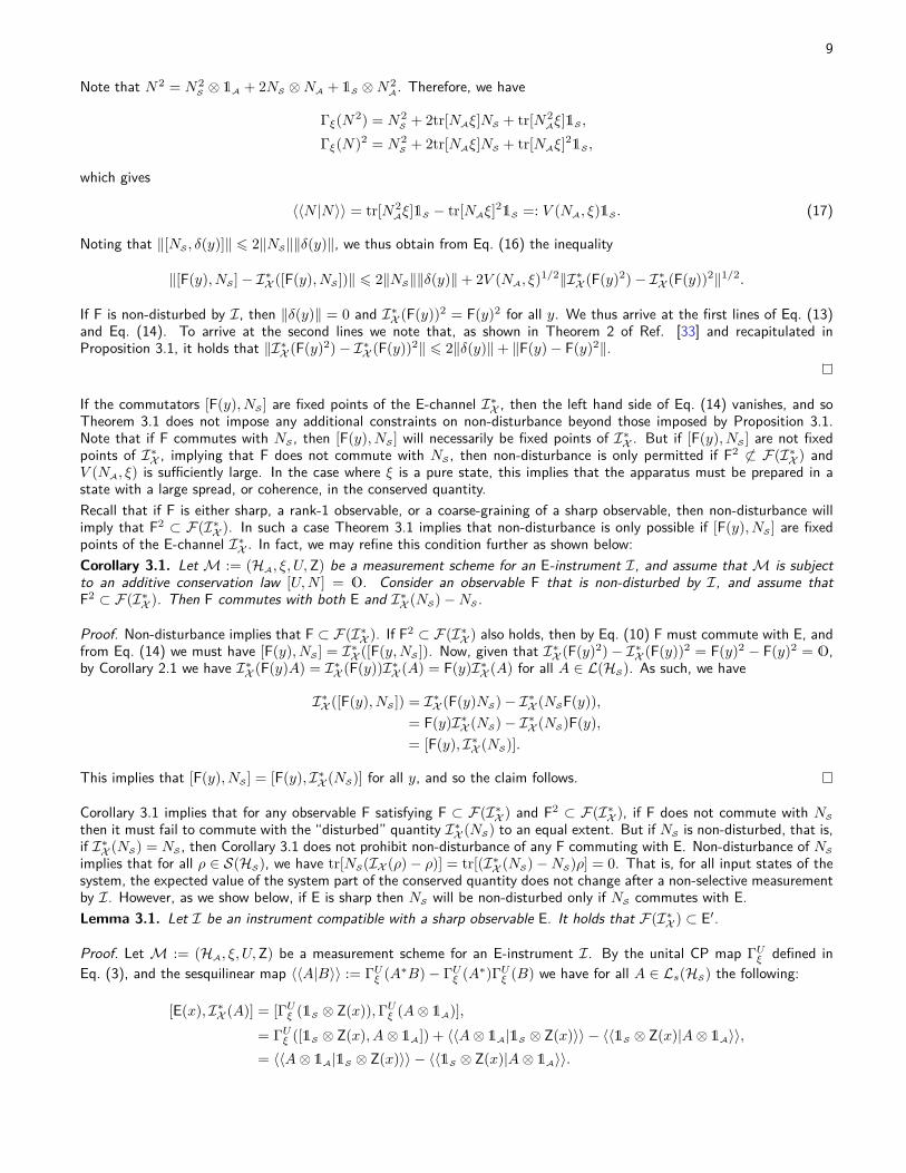
If the commutators [F(y), NS ] are fixed points of the E-channel I∗X , then the left hand side of Eq. (14) vanishes, and soTheorem 3.1 does not impose any additional constraints on non-disturbance beyond those imposed by Proposition 3.1.Note that if F commutes with NS , then [F(y), NS ] will necessarily be fixed points of I∗X . But if [F(y), NS ] are not fixedpoints of I∗X , implying that F does not commute with NS , then non-disturbance is only permitted if F2 6⊂ F(I∗X ) andV (NA, ξ) is sufficiently large. In the case where ξ is a pure state, this implies that the apparatus must be prepared in astate with a large spread, or coherence, in the conserved quantity.Recall that if F is either sharp, a rank-1 observable, or a coarse-graining of a sharp observable, then non-disturbance willimply that F2 ⊂ F(I∗X ). In such a case Theorem 3.1 implies that non-disturbance is only possible if [F(y), NS ] are fixedpoints of the E-channel I∗X . In fact, we may refine this condition further as shown below:Corollary 3.1. Let M := (HA, ξ, U,Z) be a measurement scheme for an E-instrument I, and assume that M is subjectto an additive conservation law [U,N ] = O. Consider an observable F that is non-disturbed by I, and assume thatF2 ⊂ F(I∗X ). Then F commutes with both E and I∗X (NS)−NS .

Proof. Non-disturbance implies that F ⊂ F(I∗X ). If F2 ⊂ F(I∗X ) also holds, then by Eq. (10) F must commute with E, andfrom Eq. (14) we must have [F(y), NS ] = I∗X ([F(y,NS ]). Now, given that I∗X (F(y)2)− I∗X (F(y))2 = F(y)2 − F(y)2 = O,by Corollary 2.1 we have I∗X (F(y)A) = I∗X (F(y))I∗X (A) = F(y)I∗X (A) for all A ∈ L(HS). As such, we have

I∗X ([F(y), NS ]) = I∗X (F(y)NS)− I∗X (NSF(y)),= F(y)I∗X (NS)− I∗X (NS)F(y),= [F(y), I∗X (NS)].

This implies that [F(y), NS ] = [F(y), I∗X (NS)] for all y, and so the claim follows.

Corollary 3.1 implies that for any observable F satisfying F ⊂ F(I∗X ) and F2 ⊂ F(I∗X ), if F does not commute with NS

then it must fail to commute with the “disturbed” quantity I∗X (NS) to an equal extent. But if NS is non-disturbed, that is,if I∗X (NS) = NS , then Corollary 3.1 does not prohibit non-disturbance of any F commuting with E. Non-disturbance of NS

implies that for all ρ ∈ S(HS), we have tr[NS(IX (ρ)− ρ)] = tr[(I∗X (NS)−NS)ρ] = 0. That is, for all input states of thesystem, the expected value of the system part of the conserved quantity does not change after a non-selective measurementby I. However, as we show below, if E is sharp then NS will be non-disturbed only if NS commutes with E.Lemma 3.1. Let I be an instrument compatible with a sharp observable E. It holds that F(I∗X ) ⊂ E′.

Proof. Let M := (HA, ξ, U,Z) be a measurement scheme for an E-instrument I. By the unital CP map ΓUξ defined inEq. (3), and the sesquilinear map 〈〈A|B〉〉 := ΓUξ (A∗B)− ΓUξ (A∗)ΓUξ (B) we have for all A ∈ Ls(HS) the following:

[E(x), I∗X (A)] = [ΓUξ (1S ⊗ Z(x)),ΓUξ (A⊗ 1A)],= ΓUξ ([1S ⊗ Z(x), A⊗ 1A]) + 〈〈A⊗ 1A|1S ⊗ Z(x)〉〉 − 〈〈1S ⊗ Z(x)|A⊗ 1A〉〉,= 〈〈A⊗ 1A|1S ⊗ Z(x)〉〉 − 〈〈1S ⊗ Z(x)|A⊗ 1A〉〉.

10

By the Cauchy-Schwarz inequality in Lemma 2.1, we obtain

‖[E(x), I∗X (A)]‖ 6 ‖〈〈A⊗ 1A|1S ⊗ Z(x)〉〉‖+ ‖〈〈1S ⊗ Z(x)|A⊗ 1A〉〉‖,6 2‖E(x)− E(x)2‖1/2‖I∗X (A2)− I∗X (A)2‖1/2.

If E is sharp, then A ∈ F(I∗X ) implies that A ∈ E′.Let us note that all bounded operators B ∈ L(HS) can be decomposed as B = A1 + iA2, with A1 and A2 self-adjoint operators. Clearly, if A1, A2 ∈ F(I∗X ), then B ∈ F(I∗X ). Now assume that B ∈ F(I∗X ). We thus haveI∗X (A1) = (I∗X (B) + I∗X (B∗))/2 = A1 and I∗X (A2) = (I∗X (B) − I∗X (B∗))/2i = A2. It follows that B ∈ F(I∗X ) if andonly if A1, A2 ∈ F(I∗X ). Therefore, if E is sharp then for any B ∈ L(HS), B ∈ F(I∗X ) =⇒ B ∈ E′, and so F(I∗X ) ⊂ E′.

Now consider the following scenario. Let E be a sharp observable, with the measurement of E being subject to a conservationlaw. Let F either be sharp, rank-1, or a coarse-graining of a sharp observable. Now assume that both E and F do notcommute with the conserved quantity NS . Since E is sharp, it follows from Lemma 3.1 that I∗X (NS) 6= NS . Therefore, byCorollary 3.1 F will be non-disturbed only if it commutes with both E and a non-trivial observable I∗X (NS)−NS 6= O.

4. MEASUREMENTS OF THE FIRST KIND, REPEATABILITY, AND THE WIGNER-ARAKI-YANASE THEOREM

A special instance of a non-disturbing measurement is when an E-instrument does not disturb E itself, i.e., when the statisticsof a measurement of E are not affected by a prior non-selective measurement of E. Such measurements are referred to asmeasurements of the first kind (or first-kind measurements), and the E-instrument I corresponds to a measurement of thefirst kind exactly when E ⊂ F(I∗X ) [47]. The necessary conditions for first-kindness can be obtained from Proposition 3.1and Theorem 3.1, by identifying F with E:

‖[E(x),E(y)]‖ 6 2‖E(x)− E(x)2‖1/2‖I∗X (E(y)2)− E(y)2‖1/2 ∀x, y ∈ X ,‖[E(x), NS ]− I∗X ([E(x), NS ])‖ 6 2V (NA, ξ)1/2‖I∗X (E(x)2)− E(x)2‖1/2 ∀x ∈ X .

In the absence of any conservation law, a commutative observable always admits a measurement of the first kind—recallthat for a Luders E-instrument IL, E′ ⊂ F(ILX

∗) always holds, and so if E is commutative we have E ⊂ E′ ⊂ F(ILX∗).

On the other hand, a non-commutative (and hence unsharp) observable admits a measurement of the first kind only ifE2 6⊂ F(I∗X ). In the presence of a conservation law, an observable for which [E(x), NS ] is not a fixed point of I∗X admitsa measurement of the first kind only if E2 6⊂ F(I∗X ) and V (NA, ξ) is large.A subclass of measurements of the first kind are those which are repeatable. Though it is a standard assumption in manytextbook treatments of quantum mechanics, that repeatability is a property which a measurement may or may not enjoyappeared already in Wigner’s 1952 contribution on the WAY theorem. However, within the general framework presentedthus far, repeatability corresponds merely to a very special form of state change, possible only for a privileged class ofobservables and arising only for very special measurement interactions. I is a repeatable E-instrument if

tr[Iy ◦ Ix(ρ)] = δx,ytr[Ix(ρ)] ∀ ρ ∈ S(HS), x, y ∈ X ,

which implies that

I∗x(E(y)) = δx,yE(x) ∀x, y ∈ X . (18)

In other words, if I is a repeatable instrument, then repeated measurements by I are guaranteed (with probability one)not to produce different results. We note that Eq. (18) is equivalent to I∗x(E(x)) = E(x) for all x, since if this holds thenI∗x(1S − E(x)) = E(x)− E(x) = O [48]. It is straightforward to verify that if a measurement of E is repeatable, then it isalso of the first kind, since

I∗X (E(x)) = I∗x(E(x)) = E(x).

While the converse relation does not hold in general—a measurement can be of the first kind and not repeatable—in thespecial case of sharp observables repeatability and first-kindness coincide (Theorem 1 in Ref. [47]). An observable E admitsa repeatable measurement only if it is discrete [42], and all the effects have at least one eigenvector with eigenvalue 1 [49].We now prove a useful result regarding the structure of repeatable instruments.

11

Lemma 4.1. Consider an E-instrument I. If I is repeatable, then it must satisfy

Ix(T ) = P (x)Ix(T )P (x), I∗x(A) = I∗x(P (x)AP (x)),

to hold for all x ∈ X , T ∈ T (HS), and A ∈ L(HS), where P (x) is the projection onto the eigenvalue-1 eigenspace of E(x),which satisfies

P (x)E(y) = E(y)P (x) = δx,yP (x) ∀x, y ∈ X .

Proof. Let us first write the effects of E in spectral form as E(x) =∑i a

(x)i P

(x)i , with a(x)

i ∈ [0, 1] the distinct eigenvaluesarranged in strictly decreasing order, a(x)

1 = 1 and a(x)i > a

(x)i+1, and P (x)

i the corresponding spectral projections. We maytherefore split the effects as E(x) = P (x) +Q(x), where

P (x) = P(x)1 , Q(x) =

∑i>1

a(x)i P

(x)i .

Here, P (x) is a projection operator, and specifically is the projection onto the eigenvalue-1 eigenspace of the effect E(x).Conversely, Q(x) is a positive operator whose eigenvalues are strictly smaller than 1, and Q(x) = O precisely when E(x)is a projection operator. That P (x)E(x) = E(x)P (x) = P (x) is trivial. The relations P (x)E(y) = E(y)P (x) = O forall y 6= x follow from the fact that

∑x∈X E(x) = 1, which implies that the support of P (x) must be orthogonal to the

support of E(y) for all y 6= x. To see this, let us consider ψ ∈ HS such that ψ ∈ supp(P (x)). It follows that P (x)ψ = ψ,and we thus have

(1S − P (x))ψ = (1S − E(x))ψ +Q(x)ψ,= (1S − E(x))ψ,

=∑y 6=x

E(y)ψ = ∅,

where ∅ denotes the null vector of HS . Here, in the second line we have used the fact that ψ ∈ supp(P (x)) =⇒ ψ ∈ker(Q(x)). By positivity of E(y), the above equation implies that∑

y 6=x〈ψ|E(y)ψ〉 =

∑y 6=x〈√

E(y)ψ|√

E(y)ψ〉 = 0,

which can only be satisfied if√

E(y)ψ = ∅ =⇒ E(y)ψ = ∅ for all y 6= x. We thus have ψ ∈ supp(P (x)) =⇒ ψ ∈ker(E(y))∀ y 6= x, and so the support of P (x) must be orthogonal to the support of E(y) for all y 6= x.Now consider the normalised post-measurement state ρ(x) := Ix(ρ)/tr[E(x)ρ], where tr[E(x)ρ] > 0. The repeatabilitycondition Eq. (18) implies that

tr[E(x)ρ(x)] = tr[E(x)Ix(ρ)]tr[E(x)ρ] = tr[E(x)ρ]

tr[E(x)ρ] = 1. (19)

But tr[E(x)ρ(x)] = tr[P (x)ρ(x)] + tr[Q(x)ρ(x)], and since the eigenvalues of Q(x) are all smaller than 1, thentr[E(x)ρ(x)] = 1 if and only if tr[P (x)ρ(x)] = 1. Now we wish to show that tr[P (x)ρ(x)] = 1 if and only ifρ(x) = P (x)ρ(x)P (x). The if statement is trivial, so now we shall show the only if statement. Let P be a projec-tion on HS , and define its orthogonal complement as P⊥ := 1S − P . For any state ρ, we thus have ρ = (P + P⊥)ρ.Now assume that tr[Pρ] = 1. Therefore, tr[P⊥ρ] = tr[(P⊥√ρ)∗(P⊥√ρ)] = 0, which implies that P⊥√ρ = O. Assuch, P⊥ρ = (P⊥√ρ)√ρ = O, which gives ρ = (P + P⊥)ρ = Pρ. But since both P and ρ are self-adjoint, we haveρ = Pρ = ρP . Multiplying both sides of Pρ = ρP by P from the left finally gives us ρ = PρP . We thus arrive attr[P (x)ρ(x)] = 1 ⇐⇒ ρ(x) = P (x)ρ(x)P (x). But this implies that for all T ∈ T (HS) such that tr[E(x)T ] 6= 0, we have

Ix(T )tr[E(x)T ] = P (x)Ix(T )P (x)

tr[E(x)T ] ,

which implies that Ix(T ) = P (x)Ix(T )P (x) for all T ∈ T (HS). This completes the proof.

We may now show that the condition E2 ⊂ F(I∗X ), which precludes a first-kind measurement for a non-commutativeobservable, further precludes a repeatable measurement for an unsharp observable.Lemma 4.2. Consider an E-instrument I. If I is repeatable, then I∗X (E(x)2) = E(x) for all x ∈ X .

12

Proof. Assume that I is a repeatable E-instrument. By Lemma 4.1, we have

I∗X (E(x)2) =∑y∈XI∗y (E(x)2),

=∑y∈XI∗y (P (y)E(x)2P (y)),

= I∗x(P (x)) = I∗x(1S) = E(x).

Here, we have used the fact that if I is repeatable, then I∗x(A) = I∗x(P (x)AP (x)), with P (x) the projection onto theeigenvalue-1 eigenspace of E(x), and that P (y)E(x) = δx,yP (x).

Since E(x)2 = E(x) only if E is sharp, Lemma 4.2 implies that if I is repeatable, then E(x)2 ∈ F(I∗X ) only if E is sharp.Let us examine this result in more detail. As discussed above, if I is a repeatable E-instrument then the conditional post-measurement state ρ(x) can only have support in the eigenvalue-1 eigenspace of the effect E(x). Now take the collectionof eigenvalue-1 eigenvectors of all the effects of E. If E is unsharp, then the span of these vectors will be a proper subset ofHS . It follows that if E is unsharp and I is repeatable, then F(IX ) cannot contain any faithful states. This conclusion canindependently be reached from Lemma 4.2; if F(IX ) were to contain a faithful state, then by Lemma 2.2 F(I∗X ) wouldnecessarily be a von Neumann algebra, in which case E(x) ∈ F(I∗X ) =⇒ E(x)2 ∈ F(I∗X ), and so by Lemma 4.2 I willbe repeatable only if E is sharp. On the other hand, if either E is a rank-1 observable, or a classical coarse-graining of asharp observable G, then we always have E(x) ∈ F(I∗X ) =⇒ E(x)2 ∈ F(I∗X ). But unless the rank-1 observable is sharp,or the entries of the invertible stochastic matrix M relating the effects of E with those of G are either 0 or 1 so that E isalso sharp, at least one of the effects of E will not have any eigenvectors with eigenvalue 1, so that E will not admit anyrepeatable instruments.We are now ready to prove a quantitative generalisation of the WAY theorem [2–4].Theorem 4.1 (Generalised WAY theorem). Let M := (HA, ξ, U,Z) be a measurement scheme for an E-instrument I.Assume that M is subject to an additive conservation law [U,N ] = O. If either I is repeatable, or the Yanase condition[Z, NA] = O is satisfied, then the following must hold for all x ∈ X :

‖[E(x), NS ]‖ 6 2V (NA, ξ)1/2‖E(x)− E(x)2‖1/2. (20)

Proof. Let us first assume that I is repeatable. Since repeatability implies first-kindness, which is a specific instance ofnon-disturbance, then by Theorem 3.1 and identifying F with E we must have

‖[E(x), NS ]− I∗X ([E(x), NS ])‖ 6 2V (NA, ξ)1/2‖I∗X (E(x)2)− E(x)2‖1/2 ∀x ∈ X .

By Lemma 4.2, we have I∗X (E(x)2) = E(x). By Lemma 4.1, we have

I∗X ([E(x), NS ]) = I∗X (E(x)NS)− I∗X (NSE(x)),

=∑y

I∗y (P (y)E(x)NSP (y))− I∗y (P (y)NSE(x)P (y)),

= I∗x(P (x)NSP (x))− I∗x(P (x)NSP (x)) = O.

We thus obtain Eq. (20).Now assume that the Yanase condition is satisfied. By the unital CP map defined in Eq. (3), and the conservation law, wemay write [E(x), NS ] = [ΓUξ (1S ⊗ Z(x)),ΓUξ (N)]. Using the sesquilinear mapping 〈〈A|B〉〉 := ΓUξ (A∗B)− ΓUξ (A∗)ΓUξ (B),and the Yanase condition [Z, NA] = O, we obtain

[E(x), NS ] = [ΓUξ (1S ⊗ Z(x)),ΓUξ (N)],= ΓUξ ([1S ⊗ Z(x), N ]) + 〈〈N |1S ⊗ Z(x)〉〉 − 〈〈1S ⊗ Z(x)|N〉〉,= ΓUξ (1S ⊗ [Z(x), NA]) + 〈〈N |1S ⊗ Z(x)〉〉 − 〈〈1S ⊗ Z(x)|N〉〉,= 〈〈N |1S ⊗ Z(x)〉〉 − 〈〈1S ⊗ Z(x)|N〉〉,

which gives the inequality

‖[E(x), NS ]‖ 6 ‖〈〈N |1S ⊗ Z(x)〉〉‖+ ‖〈〈1S ⊗ Z(x)|N〉〉‖. (21)

As shown in Proposition 3.1, 〈〈1S⊗Z(x)|1S⊗Z(x)〉〉 = E(x)−E(x)2, while as shown in Theorem 3.1, 〈〈N |N〉〉 = V (NA, ξ).By the Cauchy-Schwarz type inequality in Lemma 2.1, we thus obtain from Eq. (21) the inequality given in Eq. (20).

13

Note that the above theorem already contains the original WAY theorem; since the upper bound of Eq. (20) vanisheswhen E is sharp then an additive conservation law, together with either repeatability or the Yanase condition, necessitatescommutation of E with the system part of the conserved quantity. On the other hand, Theorem 4.1 illustrates the necessaryconditions that must be met when the observable does not commute with the system part of the conserved quantity andeither the measurement is repeatable, or the Yanase condition holds—the observable must be unsharp and the apparatusmust be prepared in a state with a large uncertainty in the conserved quantity. Moreover, note that under the repeatabilityassumption the bound Eq. (20) was obtained as a direct consequence of the more general non-disturbance bound shown inTheorem 3.1.Of course, while unsharpness of E and the large uncertainty of the conserved quantity in the apparatus are necessaryconditions for a repeatable measurement of E not commuting with NS , they are not sufficient. We shall now demonstratethis by a simple example, where imposing repeatability and the Yanase condition demands that the observable commuteswith the conserved quantity:Proposition 4.1. Let HS be a finite-dimensional system, and consider an unsharp, commutative observable E on HS

such that for all x ∈ X , the effect E(x) has only one eigenvector ψx with eigenvalue 1. Let M := (HA, ξ, U,Z) be ameasurement scheme for an E-instrument I, and assume that M is subject to an additive conservation law [U,N ] = O. IfI is repeatable and the Yanase condition [Z, NA] = O holds, then E commutes with NS .

Proof. We denote by Pψ := |ψ〉〈ψ| the projection on |ψ〉. By Lemma 4.1, the instrument I is repeatable only if

I∗x(A) = I∗x(PψxAPψx) = tr[APψx ]I∗x(Pψx) = tr[APψx ]I∗x(1S) = tr[APψx ]E(x),

to hold for all x ∈ X and A ∈ L(HS). Now let M := (HA, ξ, U,Z) be a measurement scheme for I. If [U,N ] = O, wehave

NS + tr[NAξ]1S = ΓUξ (NS ⊗ 1A) + ΓUξ (1S ⊗NA),

=∑y∈X

ΓUξ (NS ⊗ Z(y)) + ΓUξ (1S ⊗NA),

=∑y∈XI∗y (NS) + ΓUξ (1S ⊗NA),

=∑y∈X

tr[NSPψy ]E(y) + ΓUξ (1S ⊗NA).

Computing the commutator of both sides with E(x) thus gives

[E(x), NS ] =∑y∈X

tr[NSPψy ][E(x),E(y)] + [E(x),ΓUξ (1S ⊗NA)],

= [E(x),ΓUξ (1S ⊗NA)]. (22)

Let us write the state of the apparatus as ξ =∑n qnPφn , with φn orthogonal unit vectors, and {qn} a probability

distribution. We may thus write Γξ(·) =∑n qnV

∗φn

(·)Vφn , with Vφn : HS → HS ⊗HA, ψ 7→ ψ ⊗ φn an isometry. Now letus write Z(x) =

∑µ Pϕx,µ , with ϕx,µ orthonormal eigenvalue-1 eigenstates of Z(x). We may thus write

ΓUξ (1S ⊗NA) =∑x

ΓUξ (1S ⊗ Z(x)NAZ(x)),

=∑x,µ,ν

ΓUξ (1S ⊗ Pϕx,µNAPϕx,ν ),

=∑x,µ,ν

〈ϕx,µ|NAϕx,ν〉ΓUξ (1S ⊗ |ϕx,µ〉〈ϕx,ν |),

=∑x,µ,ν

〈ϕx,µ|NAϕx,ν〉∑n

qnV∗φnU

∗(1S ⊗ |ϕx,µ〉〈ϕx,ν |)UVφn ,

=∑x,µ,ν

〈ϕx,µ|NAϕx,ν〉∑n

qnV∗φnU

∗Vϕx,µV∗ϕx,νUVφn . (23)

In the first line we have used the Yanase condition, and in the final line we have used the fact that VφV ∗φ′ = 1S ⊗ |φ〉〈φ′|.Here, for each x the set {Kx,µ,n := √qnV ∗ϕx,µUVφn} is a Kraus representation for the operation Ix. In what follows, we willignore the subscript n, as this can be accounted for by allowing multiplicities in the appearance of the terms 〈ϕx,µ|NAϕx,ν〉.

14

Since E is commutative, we may write all effects as

E(x) =∑i

λ(x)i Pψi , (24)

with {ψi} an orthonormal basis of HS . It is simple to see that

Kx,i :=√λ

(x)i |ψx〉〈ψi| (25)

is a Kraus representation for Ix. In fact, it is a minimal Kraus representation since Kx,i are linearly independent. As shownin [50] there exists an isometry [uµ,i ∈ C], satisfying

∑µ u∗µ,iuµ,j = δi,j , such that Kx,µ =

∑i uµ,iKx,i. Evaluating the

sum in Eq. (23) for each x individually gives∑µ,ν

〈ϕx,µ|NAϕx,ν〉K∗x,µKx,ν =∑µ,ν

〈ϕx,µ|NAϕx,ν〉(∑

i

uµ,iKx,i

)∗(∑j

uν,jKx,j

),

=∑µ,ν,i,j

u∗µ,iuν,j〈ϕx,µ|NAϕx,ν〉K∗x,iKx,j ,

=∑i,j

〈ϕx,i|NAϕx,j〉K∗x,iKx,j , (26)

where ϕx,i :=∑µ uµ,iϕx,µ is a superposition of the eigenvalue-1 eigenstates of Z(x), and hence is also an eigenvalue-1

eigenstate of Z(x). But Given that [uµ,i] is an isometry, we have

〈ϕx,i|ϕx,j〉 =∑µ,ν

u∗µ,iuν,j〈ϕx,µ|ϕx,ν〉,

=∑µ

u∗µ,iuµ,j = δi,j .

In the second line, we have used the fact that 〈ϕx,µ|ϕx,ν〉 = δµ,ν . Therefore, ϕx,i are orthonormal eigenvalue-1 eigenstatesof Z(x). By the Yanase condition, ϕx,i are eigenstates of NA, and so 〈ϕx,i|NAϕx,j〉 = 0 if i 6= j. As such, by Eq. (23),Eq. (25), and Eq. (26), we obtain

ΓUξ (1S ⊗NA) =∑x,i

〈ϕx,i|NAϕx,i〉K∗x,iKx,i,

=∑x,i

〈ϕx,i|NAϕx,i〉λ(x)i Pψi .

It follows from Eq. (24) that [E(x),ΓUξ (1S ⊗NA)] = O, and hence by Eq. (22) [E(x), NS ] = O.

5. FIXED POINTS AND MEASUREMENT DISTURBANCE

In Sec. 3 we obtained quantitative bounds for non-disturbance of an observable F by an E-instrument I implemented inthe presence of an additive conservation law. We saw that if F2 is contained in the fixed point set of I∗X—guaranteedby non-disturbance if F is either sharp, a rank-1 observable, or a coarse-graining of a sharp observable—then it must holdthat F commutes with E, and [F(y), NS ] = I∗X ([F(y), NS ]). Now we shall see that the structure of the Schrodinger picturechannel fixed points, F(IX ), will impose similar constraints on non-disturbance for an arbitrary observable F.

5.1. Faithful fixed points

Recall from Lemma 2.2 that if the fixed-points of the E-channel IX contains a faithful state, then F(I∗X ) is a von Neumannalgebra. In such a case it follows that for any observable F, non-disturbance of F guarantees that F2 ⊂ F(I∗X ). Therefore,by Proposition 3.1 F will be non-disturbed only if it commutes with E, and by Theorem 3.1 the conservation law furtherimposes that [F(y), NS ] = I∗X ([F(y), NS)]) must hold. Furthermore, I is a measurement of the first kind only if E iscommutative, while by Lemma 4.2 if I is repeatable, then E must be sharp, and hence by Theorem 4.1 E must commutewith NS . Below, we shall show that further restrictions must hold. First, let us prove a useful lemma.

15

Lemma 5.1. Let M := (HA, ξ, U,Z) be a measurement scheme for an E-instrument I. If F(I∗X ) is a von Neumannalgebra, then F(I∗X ) ⊂ E′. If additionallyM is subject to an additive conservation law [U,N ] = O, then for all A ∈ L(HS),A ∈ F(I∗X ) =⇒ [A,NS ] ∈ E′.

Proof. All C ∈ L(HS) can be written as C = A+ iB, where A and B are self-adjoint operators. Assume that C ∈ F(I∗X ).Since I∗X (A) = (I∗X (C) + I∗X (C∗))/2 = A and I∗X (B) = (I∗X (C) − I∗X (C∗))/2i = B, it clearly follows that A ∈ F(I∗X )and B ∈ F(I∗X ). Now assume that F(I∗X ) is a von Neumann algebra. Note that if a self-adjoint operator is in a vonNeumann algebra, then so too are its spectral projections. As such, if A has the spectral decomposition A =

∑n λnPn,

then A ∈ F(I∗X ) implies Pn ∈ F(I∗X ) for all n. For each n consider an observable {I∗x(Pn), I∗x(1S − Pn) : x ∈ X} whichinduces a joint measurement of E and P := {Pn,1S − Pn}. As P is sharp, [Pn,E] = O follows. The same argument holdsfor B. It follows that F(I∗X ) ⊂ E′.Now let us assume that M is subject to an additive conservation law. Let us first recall that for all A ∈ L(HS), we haveI∗X (A) = ΓUξ (A⊗ 1A), where ΓUξ is the unital CP map defined in Eq. (3). The conservation law implies that

NS + tr[NAξ]1S = ΓUξ (NS ⊗ 1A) + ΓUξ (1S ⊗NA).

Since F(I∗X ) is a von Neumann algebra, it follows that A ∈ F(I∗X ) =⇒ A∗A ∈ F(I∗X ) which, by Corollary 2.1, impliesthat AΓUξ (B) = ΓUξ (A⊗ 1A)ΓUξ (B) = ΓUξ ((A⊗ 1A)B) for all B ∈ Ls(HS ⊗HA). Therefore, for all A ∈ F(I∗X ) we have

[A,NS ] = [ΓUξ (A⊗ 1A),ΓUξ (NS ⊗ 1A)] + [ΓUξ (A⊗ 1A),ΓUξ (1S ⊗NA)],= ΓUξ ([A,NS ]⊗ 1A) + ΓUξ ([A⊗ 1A,1S ⊗NA]),= ΓUξ ([A,NS ]⊗ 1A) = I∗X ([A,NS ]).

Consequently, we see that A ∈ F(I∗X ) =⇒ [A,NS ] ∈ F(I∗X ) =⇒ [A,NS ] ∈ E′.

We are now ready to prove the following:Theorem 5.1. Let M := (HA, ξ, U,Z) be a measurement scheme for an E-instrument I. Assume that M is subject toan additive conservation law [U,N ] = O, and that F(I∗X ) is a von Neumann algebra. The following holds:

(i) I does not disturb an observable F only if E commutes with both F and {[F(y), NS ] : y ∈ Y}.(ii) I is a measurement of the first kind only if E is a commutative observable that commutes with NS .(iii) I is repeatable only if E is sharp and commutes with NS .

Proof. Let us first prove (i). I does not disturb F only if F ⊂ F(I∗X ). But by Lemma 5.1 F(I∗X ) ⊂ E′, and so F mustcommute with E. Moreover, given the conservation law Lemma 5.1 gives the implication F(y) ∈ F(I∗X ) =⇒ [F(y), NS ] ∈E′.Now let us prove (ii). I is a measurement of the first kind only if E ⊂ F(I∗X ). But by Lemma 5.1 F(I∗X ) ⊂ E′, and so Emust be commutative. Consider the spectral decomposition of an effect of E as E(x) =

∑n λnPn. Since F(I∗X ) is a von

Neumann algebra, then E(x) ∈ F(I∗X ) =⇒ Pn ∈ F(I∗X ) for all n, and by Lemma 5.1 Pn ∈ F(I∗X ) =⇒ [Pn, NS ] ∈ E′.But [A,E(x)] = O only if [A,Pn] = O for all n. As such, we must have [[Pn, NS ], P⊥n ] = O, where P⊥n := 1S − Pn.But this implies that [PnNS − NSPn, P

⊥n ] = PnNSP

⊥n + P⊥n NSPn = O. Multiplying from the left by Pn, we thus have

PnNSP⊥n = PnNS(1S − Pn) = O, and so PnNS = PnNSPn. Since the right hand side is self-adjoint, it follows that

PnNS = NSPn. Since this relation holds for all spectral projections of all effects of E, it follows that E must commute withNS .Finally, let us prove (iii). Since repeatability implies first-kindness, then by (ii) E must commute with NS . Sharpness of Efollows from Lemma 4.2 and the fact that if F(I∗X ) is a von Neumann algebra, then E ⊂ F(I∗X ) implies that E2 ⊂ F(I∗X ).

We shall now give some examples where F(IX ) necessarily contains a faithful state, so that F(I∗X ) is necessarily a vonNeumann algebra, and so the implications of Theorem 5.1 will always hold.Lemma 5.2. Consider the Luders E-instrument IL, defined in Eq. (1). If either (i) HS ' Cd, or (ii) E is commutative,then F(ILX

∗) is a von Neumann algebra.

Proof. Let us first consider (i). Define the complete mixture π := 1S/d, which is faithful. It follows trivially that ILX (π) = π,and so F(ILX ) contains a faithful state π. Now let us consider (ii). If E is commutative, it follows that there exists anorthonormal basis {φn} where φn are eigenstates of all effects E(x). Define a (potentially unbounded) self-adjoint operator

16

AE :=∑n nPφn . It follows that e−AE :=

∑n e−nPφn is positive and trace-class, with trace in the infinite-dimensional case

given by the limit tr[e−AE ] = limN→∞∑Nn=1 e

−n = 1/(e− 1). Consequently, ω := e−AE/tr[e−AE ] is a faithful state. Butsince [E, ω] = O, we have ILX (ω) = ω (trace-norm converging), and once again F(ILX ) contains a faithful state. In eithercase, by Lemma 2.2 F(ILX

∗) is a von Neumann algebra.

Recall that F(I∗X ) is an algebra if F(I∗X ) = {Ki,K∗i }′, with {Ki} a Kraus representation of IX [35]. But for a Luders

instrument, we have {Ki,K∗i }′ = {

√E(x)}′ = E′. While E′ ⊂ F(ILX

∗) always holds, it was observed that in infinite-dimensional systems there exists E for which F(ILX

∗) 6⊂ E′ [51]. However, it was shown in [46] that for two-valuedobservables, it always holds that F(ILX

∗) = E′. Since two-valued observables are commutative, this led to the conjecturethat the fixed point set of the Luders E-channel is the commutant of E for all commutative observables [52], which waslater proven to be the case [53, 54]. We now highlight an interesting consequence of Lemma 5.2.Corollary 5.1. Let E be a commutative observable, with M := (HA, ξ, U,Z) a measurement scheme for the LudersE-instrument IL. If [U,N ] = O, with N an additive quantity, then E must commute with NS .

Proof. If E ⊂ E′, then E ⊂ F(ILX∗), and so the Luders instrument for a commutative observable is a measurement of the

first kind. But if E ⊂ E′, then F(ILX∗) = E′ is a von Neumann algebra. It follows from Theorem 5.1 that E must commute

with NS .

Lemma 5.3. Consider an arbitrary E-instrument I on a qubit, HS ' C2. Assume that I does not disturb a non-trivialobservable F. It follows that F(I∗X ) is a von Neumann algebra.

Proof. As shown in Proposition 6 in Ref. [26], if HS ' C2, then either F(IX ) contains a faithful state, or F(I∗X ) onlycontains operators that are proportional to 1S . But if F(I∗X ) only contains operators that are proportional to 1S , the onlyobservables that are non-disturbed are trivial. As such, F(IX ) must contain a faithful state, and by Lemma 2.2 F(I∗X ) isa von Neumann algebra.

Lemma 5.4. Assume that HS ' Cd, and let G := {G(z) : z = 1, . . . , d} be a rank-1 sharp observable. Let M be aninvertible stochastic matrix such

F(y) =∑z

My,zG(z), G(z) =∑y

M−1z,yF(y).

The E-instrument I does not disturb F only if F(I∗X ) is a von Neumann algebra.

Proof. Non-disturbance of F implies that G ⊂ F(I∗X ). Since G(z) is a rank-1 projection, it follows that

tr[G(z)IX (G(z))] = tr[I∗X (G(z))G(z)] = tr[G(z)G(z)] = tr[G(z)] = 1,

and so IX (G(z)) = G(z). Consequently, we may construct the faithful state ρ =∑z pzG(z) with pz > 0 and

∑z pz = 1,

so that ρ ∈ F(IX ). By Lemma 2.2, F(I∗X ) is a von Neumann algebra.

5.2. Non-faithful fixed points

Due to the Schauder–Tychonoff fixed point theorem [55], all channels Φ : T (HS)→ T (HS) contain at least one fixed point.However, it may be that none of these are faithful. In such a case, the fixed point set of the dual channel will no longernecessarily be a von Neumann algebra, but rather forms an operator space. This setting has been much less investigated,and its analysis forms the first part of this section. While the discussion thus far has been applicable for infinite-dimensionalsystems—except in some examples—in this section we shall always assume that d := dim(HS) <∞.Consider a channel Φ : T (HS) → T (HS), and its dual in the Heisenberg picture Φ∗ : L(HS) → L(HS). We define thechannel Φ∗av by

Φ∗av(A) := limN→∞

1N

N∑n=1

Φ∗n(A),

to hold for all A ∈ L(HS), and Φav is similarly defined. Note that this limit exists as d < ∞. According to the Jordandecomposition theorem, Φ∗ is represented as a summation of projections onto eigenspaces multiplied by the correspondingeigenvalues, and nilpotent operators whose eigenspaces are invariant subspaces; Φ∗av corresponds to the projection onto thesubspace with eigenvalue 1.

17

The fixed point set F(Φ∗) forms an operator space, i.e., a norm-closed vector subspace of the codomain of F(Φ∗). Φ∗av isa CP projection onto the operator space F(Φ∗), and it satisfies the following properties:

(i) Φ∗ ◦ Φ∗av = Φ∗av ◦ Φ∗ = Φ∗av ◦ Φ∗av = Φ∗av.(ii) Φ∗av(L(HS)) = F(Φ∗av) = F(Φ∗).

To prove (ii), we note that F(Φ∗) ⊆ F(Φ∗av) is trivial. Conversely, let A ∈ F(Φ∗av), and so by (i) we have Φ∗(A) = Φ∗ ◦Φ∗av(A) = Φ∗av(A) = A, and therefore A ∈ F(Φ∗). Finally for any B ∈ L(HS), Φ∗av(B) satisfies Φ∗av ◦ Φ∗av(B) = Φ∗av(B),and thus Φ∗av(B) ∈ F(Φ∗av). We note that the same properties hold for Φav, that is, Φ◦Φav = Φav ◦Φ = Φav ◦Φav = Φav,and Φav(T (HS)) = F(Φav) = F(Φ).Lemma 5.5. Let P be the minimal projection on the support of ρ0 := Φav( 1

d1S) ∈ F(Φav) = F(Φ), and P⊥ := 1S − Pits orthogonal complement. The following holds:

(i) Φ∗av(P ) = 1S and Φ∗av(P⊥) = O.(ii) For all A > O, Φ∗av(P⊥AP⊥) = O.(iii) For all A ∈ L(HS), Φ∗av(AP⊥) = Φ∗av(P⊥A) = O.(iv) For all A ∈ L(HS), Φ∗av(A) = Φ∗av(PAP ).(v) P = min{P ′| P ′ is a projection, P ′ρP ′ = ρ ∀ ρ ∈ F(Φ)}, that is, P is the minimal support projection on the fixed

points of Φ.(vi) Φ∗(P ) > P and Φ∗(P⊥) 6 P⊥.

Proof. (i) Since Φ∗av is a unital CP map, and O < P 6 1S , it follows that O < Φ∗av(P ) 6 1S . But tr[Φ∗av(P )] =d tr[ρ0P ] = d, and so Φ∗av(P ) = 1S . It trivially follows that Φ∗av(P⊥) = Φ∗av(1S)− Φ∗av(P ) = 1S − 1S = O.

(ii) Since A is positive and Φ∗av is a CP map, it follows from (i) that O 6 Φ∗av(P⊥AP⊥) 6 ‖A‖Φ∗av(P⊥) = O.(iii) By Kadison’s inequality and (ii), it follows that O = Φ∗av(P⊥A∗AP⊥) > Φ∗av(P⊥A∗)Φ∗av(AP⊥) > O.(iv) By (iii), for all A ∈ L(HS) we have Φ∗av(A) = Φ∗av((P + P⊥)A(P + P⊥)) = Φ∗av(PAP ).(v) By (iv), for all A ∈ L(HS) and ρ ∈ F(Φ) we have tr[Aρ] = tr[Φ∗av(A)ρ] = tr[Φ∗av(PAP )ρ] = tr[APρP ], and so

ρ ∈ F(Φ) =⇒ ρ = PρP . Since P is the minimal support projection of ρ0 ∈ F(Φ), the claim follows.(vi) Since P is the smallest projection satisfying ρ0 = Pρ0P , while tr[ρ0Φ∗(P )] = tr[Φ(ρ0)P ] = tr[ρ0P ] = 1, it follows

that Φ∗(P ) = P + Q > P , where Q > O is a positive operator with orthogonal support to P . We thus also haveΦ∗(P⊥) = P⊥ −Q 6 P⊥.

Let us now define the maps

Φ∗av,P (A) := PΦ∗av(A)P, Φ∗P (A) := PΦ∗(A)P. (27)

Note that Φ∗av,P : L(HS) → L(HS) is not necessarily unital, since Φ∗av,P (1S) = P 6 1S . However, the restriction ofΦ∗av,P to L(PHS)→ L(PHS), which is also denoted by Φ∗av,P , is a unital CP map, since P is the identity in L(PHS) andΦ∗av,P (P ) = P . The same holds for Φ∗P .Lemma 5.6. (i) Φ∗av,P is a completely positive projection L(HS)→ L(PHS).(ii) F(Φ∗av,P ) = Φ∗av,P (L(PHS)) is a (unital) ∗-algebra in L(PHS).(iii) The map Φ∗av is a bijection from the ∗-algebra F(Φ∗av,P ) to F(Φ∗).(iv) The inverse of Φ∗av : F(Φ∗av,P )→ F(Φ∗) is AdP : A 7→ PAP .

Proof. (i) Recall from item (iv) of Lemma 5.5 that for all A ∈ L(HS), it holds that Φ∗av(A) = Φ∗av(PAP ). It follows that

Φ∗av,P ◦ Φ∗av,P (A) = Φ∗av,P ◦ Φ∗av(A) = PΦ∗av ◦ Φ∗av(A)P = PΦ∗av(A)P = Φ∗av,P (A).

(ii) Recall that the CP map Φ∗av,P : L(PHS) → L(PHS) is unital, where the unit in L(PHS) is P . Moreover, ρ0 is afaithful fixed point of Φav,P in T (PHS), so by Lemma 2.2, the fixed point set F(Φ∗av,P ) ⊂ L(PHS) is a unital ∗-algebra. Now by (i) it follows that for any A ∈ L(PHS), Φ∗av,P (A) ∈ F(Φ∗av,P ) and so Φ∗av,P (L(PHS)) ⊆ F(Φ∗av,P ).The converse is trivial.

(iii) For all A ∈ F(Φ∗) = F(Φ∗av), there exists an operator PAP ∈ F(Φ∗av,P ) such that Φ∗av(PAP ) = Φ∗av(A) = A.Therefore, Φ∗av is surjective. Now assume that there exists A ∈ F(Φ∗av,P ) such that Φ∗av(A) = O. This implies thatA = Φ∗av,P (A) = PΦ∗av(A)P = O. Therefore, Φ∗av is injective.

18

(iv) Follows from above.

Proposition 5.1. Consider the maps Φ∗av,P and Φ∗P defined in Eq. (27). It holds that F(Φ∗av,P ) = F(Φ∗P ) = PF(Φ∗)P .

Proof. We first prove that F(Φ∗av,P ) = PF(Φ∗)P . For A ∈ F(Φ∗) = F(Φ∗av), PAP satisfies Φ∗av,P (PAP ) =PΦ∗av(PAP )P = PΦ∗av(A)P = PAP . Thus PAP ∈ F(Φ∗av,P ), and so PF(Φ∗)P ⊆ F(Φ∗av,P ). On the other hand,since F(Φ∗av,P ) = Φ∗av,P (L(PHS)), all fixed points of Φ∗av,P can be constructed as Φ∗av,P (PAP ) = PΦ∗av(A)P , and sinceΦ∗av(A) ∈ F(Φ∗av) = F(Φ∗), we have F(Φ∗av,P ) ⊆ PF(Φ∗)P . Thus the claim F(Φ∗av,P ) = PF(Φ∗)P follows.Now we shall prove that F(Φ∗av,P ) = F(Φ∗P ). First, let us note that by property (vi) of Lemma 5.5, for any A > O we haveO 6 Φ∗(P⊥AP⊥) 6 ‖A‖Φ∗(P⊥) 6 ‖A‖P⊥, and so Φ∗P (P⊥AP⊥) = PΦ∗(P⊥AP⊥)P = O. By Kadison’s inequality wethus have for all A ∈ L(HS)

O = Φ∗P (P⊥A∗AP⊥) > PΦ∗(P⊥A∗)Φ∗(AP⊥)P > O,

and hence PΦ∗(P⊥A) = Φ∗(AP⊥)P = O for all A ∈ L(HS). Since A = (P + P⊥)A(P + P⊥), it follows thatΦ∗P (A) = Φ∗P (PAP ) for all A ∈ L(HS). Now let us define the CP map Φ∗P,av : L(HS)→ L(PHS) as

Φ∗P,av(A) := limN→∞

1N

N∑n=1

Φ∗nP (A).

But since Φ∗P (A) = Φ∗P (PAP ), it follows that Φ∗2P (A) = Φ∗P (PΦ∗(A)P ) = Φ∗P ◦Φ∗(A) = PΦ∗2(A)P for all A. It followsthat

Φ∗P,av(A) = limN→∞

1N

N∑n=1

PΦ∗n(A)P = PΦ∗av(A)P =: Φ∗av,P (A).

We see that as with the relationship between Φ∗ and Φ∗av, we have Φ∗P ◦ Φ∗av,P = Φ∗av,P ◦ Φ∗P = Φ∗av,P ◦ Φ∗av,P = Φ∗av,P .That F(Φ∗P ) ⊆ F(Φ∗av,P ) is trivial, so now we show the converse. Assume that A = Φ∗av,P (A) ∈ F(Φ∗av,P ). It follows thatΦ∗P (A) = Φ∗P ◦ Φ∗av,P (A) = Φ∗av,P (A) = A, and so A ∈ F(Φ∗P ). We therefore have F(Φ∗av,P ) = F(Φ∗P ).

We are now ready to address the question of measurement disturbance. As before, let I := {Ix : x ∈ X} be an E-compatibleinstrument, with IX :=

∑x Ix the corresponding channel induced by a nonselective measurement. We define

I∗av(A) := limN→∞

1N

N∑n=1I∗nX (A), I∗av,P (A) := PI∗av(A)P, I∗P (A) := PI∗X (A)P,

where as in Lemma 5.5, P is the minimal support projection on ρ0 := Iav( 1d1S), which corresponds with the minimal

projection on the support of F(IX ). By Lemma 5.6 and Proposition 5.1, F(I∗av,P ) = F(I∗P ) = PF(I∗X )P is a vonNeumann elgebra in L(PHS). We define by PEP := {PE(x)P : x ∈ X} the restriction of E to an observable on PHS ,which satisfies

∑x PE(x)P = P , and (PEP )′ := {A ∈ L(PHS) : [PE(x)P,A] = O∀x} denotes the commutant of PEP

in L(PHS). PFP is similarly defined.Before generalising Theorem 5.1 for the case where F(IX ) does not contain any faithful states, let us first prove ageneralisation of Lemma 5.1.Lemma 5.7. Let M := (HA, ξ, U,Z) be a measurement scheme for an E-instrument I. It follows that PF(I∗X )P ⊂(PEP )′. If M is subject to an additive conservation law [U,N ] = O, then additionally A ∈ PF(I∗X )P =⇒ [A,PNSP ] ∈(PEP )′.

Proof. Let A = PAP be a self-adjoint operator with the spectral decomposition A =∑n λnRn. Since PF(I∗X )P is a von

Neumann algebra in L(PHS), A ∈ PF(I∗X )P =⇒ Rn ∈ PF(I∗X )P for all n. For each n, define the sharp observable onPHS as R := {Rn, P −Rn}. It follows that {PI∗x(Rn)P, PI∗x(1S −Rn)P : x ∈ X} is a joint observable for PEP and R.Since R is sharp, it follows that Rn must commute with PEP . Therefore, PF(I∗X )P ⊂ (PEP )′.Now let us assume that M is subject to an additive conservation law [U,N ] = O. By Eq. (3) define the CP mapΓUξ,P : L(HS⊗HA)→ L(PHS), B 7→ PΓUξ (B)P . We note that ΓUξ,P is unital when restricted to L(PHS⊗HA)→ L(PHS),

19

and it holds that ΓUξ,P (B) = ΓUξ,P ((P ⊗ 1A)B(P ⊗ 1A)). We thus have I∗P (A) = I∗P (PAP ) = ΓUξ,P (PAP ⊗ 1A) for allA ∈ L(HS). The conservation law implies that PΓξ(N)P = ΓUξ,P (N) = ΓUξ,P ((P ⊗ 1A)N(P ⊗ 1A)), and so

PNSP + tr[NAξ]P = ΓUξ,P (PNSP ⊗ 1A) + ΓUξ,P (P ⊗NA).

Now assume that A = ΓUξ,P (A ⊗ 1A) ∈ PF(I∗X )P . Since PF(I∗X )P is a von Neumann algebra in L(PHS), thenA∗A ∈ PF(I∗X )P and by Corollary 2.1 AΓUξ,P (B) = ΓUξ,P (A ⊗ 1A)ΓUξ,P (B) = ΓUξ,P ((A ⊗ 1A)B) for all self-adjointB ∈ Ls(PHS ⊗HA). It follows that

[A,PNSP ] = [ΓUξ,P (A⊗ 1A),ΓUξ,P (PNSP ⊗ 1A)] + [ΓUξ,P (A⊗ 1A),ΓUξ,P (P ⊗NA)],= ΓUξ,P ([A⊗ 1A, PNSP ⊗ 1A]) + ΓUξ,P ([A⊗ 1A, P ⊗NA]),= I∗P ([A,PNSP ]).

Since [A,PNSP ] ∈ F(I∗P ) = PF(I∗X )P , it follows that [A,PNSP ] ∈ (PEP )′.

We are now ready to generalise Theorem 5.1.Theorem 5.2. Let M := (HA, ξ, U,Z) be a measurement scheme for an E-instrument I, and assume that M is subjectto an additive conservation law [U,N ] = O. The following will hold:

(i) I does not disturb an observable F only if PEP commutes with both PFP and {[PF(y)P, PNSP ] : y ∈ Y}.(ii) I is a measurement of the first kind only if PEP is commutative and commutes with PNSP .(iii) I is repeatable only if PEP is sharp and commutes with PNSP .

Proof. (i) If F ⊂ F(I∗X ), it follows that I∗P (PF(y)P ) = I∗P (F(y)) = PI∗X (F(y))P = PF(y)P , and so PFP ⊂ PF(I∗X )P .The claims follow from Lemma 5.7.(ii) As with (i), E ⊂ F(I∗X ) implies that PEP ⊂ PF(I∗X )P . By Lemma 5.7 PEP ⊂ (PEP )′, and so PEP must becommutative. That PEP must commute with PNSP follows from similar arguments as in Theorem 5.1, item (ii).(iii) Commutativity of PEP with PNSP follows from (ii) and the fact that repeatability implies first-kindness. Sharpnessof PEP follows from the fact that the fixed points of a repeatable instrument can only have support in the eigenvalue-1eigenspaces of E, as shown in Lemma 4.1.

We shall now show that if I does not disturb a non-trivial observable, then there exists a repeatable instrument J measuringa third observable such that a non-selective measurement by I between the repeated measurements of J does not destroythe repeatability property of J .Proposition 5.2 (Nondisturbance implies repeatability). Consider an E-instrument I which does not disturb a non-trivialobservable F. There exists an observable G := {G(z) : z ∈ Z} admitting a repeatable instrument J such that, for allρ ∈ S(HS) and y, z ∈ Z,

tr[Jy ◦ IX ◦ Jz(ρ)] = tr[Jy ◦ Jz(ρ)] = δy,ztr[G(z)ρ].

Proof. Suppose that a non-trivial observable F := {F(y) : y ∈ Y} is nondisturbed by I, i.e, F ⊂ F(I∗X ) = F(I∗av). Giventhat F(I∗av,P ) = PF(I∗X )P (see Proposition 5.1), this implies that PF(y)P ∈ F(I∗av,P ). That F is non-trivial implies thatthere must be a y for which PF(y)P is not proportional to P , since if that were the case every PF(y)P could be writtenas PF(y)P = cyP with some cy > 0. This would imply that F(y) = I∗av(F(y)) = I∗av(PF(y)P ) = cyI∗av(P ) = cy1S , andso F would be a trivial observable. Therefore PF(I∗av)P = F(I∗av,P ) is a nontrivial von Neumann algebra in L(PHS), andthere exists a family of projections R := {R(z) : z ∈ Z} ⊂ F(I∗av,P ) satisfying R(z)R(y) = δz,yR(z) and

∑z R(z) = P .

We may consider R as a sharp observable on PHS . This observable defines a (generally unsharp) observable G := {G(z) =I∗av(R(z)) : z ∈ Z} on HS , where

∑z G(z) = I∗av(P ) = 1S , which is not disturbed by I∗X . Each effect of G has at

least one eigenvector with eigenvalue 1, since PG(z)P = I∗av,P (R(z)) = R(z) holds. It follows that G admits a repeatableinstrument J := {Jz : z ∈ Z}, where by Lemma 4.1 Jz(ρ) = R(z)Jz(ρ)R(z). Since G ⊂ F(I∗X ), we have

tr[Jy ◦ IX ◦ Jz(ρ)] = tr[J ∗z ◦ I∗X (G(y))ρ] = tr[J ∗z (G(y))ρ] = δy,ztr[G(z)ρ].

In particular, for an arbitrary input state ρ, let us define the states {ρ(z) = Jz(ρ)/tr[G(z)ρ] : tr[G(z)ρ] > 0}. These statesare mutually orthogonal, as they satisfy ρ(z) = R(z)ρ(z)R(z), and are hence perfectly distinguishable by a G measurement.The above proposition implies that the states IX (ρ(z)) continue to be distinguishable by a G measurement.

20

Let us now consider the case of first-kind measurements in more detail. Assume that the E-instrument I is a measurementof the first kind, that is, E ⊂ F(I∗X ). By Proposition 5.2, if E is non-trivial then there exists a family of projectionsR := {R(z) : z ∈ Z} ⊂ F(I∗av,P ), satisfying

∑z R(z) = P . But by (ii) in Theorem 5.2, it must hold that PEP ⊂

F(I∗av,P ) ⊂ (PEP )′. Since PEP ⊂ (PEP )′′ always holds, while (PEP )′′ is the smallest von Neumann algebra containingPEP , it follows that (PEP )′′ ⊂ (PEP )′ = ((PEP ′′))′, and so (PEP )′′ is a commutative von Neumann algebra. It followsthat R can be chosen so as to simultaneously diagonalise all PE(x)P . We therefore arrive at the following theorem.Theorem 5.3. An observable E admits a measurement of the first kind only if E is described by a post-processing of anorm-1 observable G := {G(z) = I∗av(R(z)) : z ∈ Z}, where G is called a norm-1 observable if ‖G(z)‖ = 1 for every z forwhich G(z) 6= O.

Proof. Since R simultaneously diagonalises all PE(x)P , we may write PE(x)P =∑z p(x|z)R(z), where {p(x|z)} satisfies

p(x|z) > 0 and∑x p(x|z) = 1. We obtain E(x) = I∗av(PE(x)P ) =

∑z p(x|z)I∗av(R(z)) =:

∑z p(x|z)G(z). As shown in

Proposition 5.2, PG(z)P = R(z), and so G(z) has at least one eigenvector with eigenvalue 1. It follows that ‖G(z)‖ = 1.

Finally, we present a quantitative version of the WAY theorem for measurements of the first kind. Consider a measurementscheme M := (HA, ξ, U,Z) for a nontrivial observable E with the instrument I. Assume that I is a measurement ofthe first kind, and that M is subject to an additive conservation law [U,N ] = O where N = NS ⊗ 1A + 1S ⊗ NA. Wemay assume E to be a binary observable E := {E(1),E(2) = 1S − E(1)}, which can be constructed by coarse-graininga general observable. Since I is a measurement of the first kind, then by Theorem 5.3 we have E(1) =

∑z p(1|z)G(z)

and E(2) =∑z p(2|z)G(z), where {G(z) : z ∈ Z} is an observable satisfying ‖G(z)‖ = 1 for each z, while {p(1|z)} and

{p(2|z)} are a family of non-negative numbers satisfying p(1|z) + p(2|z) = 1. Now we introduce a pair of normalised,orthogonal vectors ψz and ψy satisfying G(z)ψz = ψz and G(y)ψy = ψy for some z and y. Proposition 5.2 shows thatIX (Pψz ) and IX (Pψy ) are perfectly distinguishable by a G measurement.We may now apply a result obtained in Ref. [9] to find

|〈ψz|NSψy〉| 6 ‖NS‖F(Λ(Pψz ),Λ(Pψy )

),

where Λ : T (HS) → T (HA), ρ 7→ trS [U(ρ ⊗ ξ)U∗] is the conjugate channel to IX , describing the reduced state of theapparatus after the measurement interaction, while F (ρ1, ρ2) is the fidelity between ρ1 and ρ2. As tr[Z(j)Λ(ρ)] = tr[E(j)ρ]for j = 1, 2 holds, the fidelity is bounded as

F(Λ(Pψz ),Λ(Pψy )

)6∑j=1,2

〈ψz|E(j)ψz〉1/2〈ψy|E(j)ψy〉1/2 =∑j=1,2

p(j|z)1/2p(j|y)1/2.

Now we choose z and y so that z = argmaxz′p(1|z′) and y = argminy′p(1|y′). That is, z is chosen so that p(1|z) assumesthe largest value, while y is chosen so that p(1|y) assumes the smallest value. In this case one can show that

p(1|z) = ‖E(1)‖, p(1|y) = 1− ‖1S − E(1)‖,p(2|z) = 1− ‖E(1)‖, p(2|y) = ‖1S − E(1)‖.

Let us first prove p(1|z) = ‖E(1)‖. Since E(1) is positive, by the C∗ identity it holds that ‖E(1)‖ = ‖√

E(1)‖2 =sup‖ψ‖=1〈ψ|E(1)ψ〉. ‖E(1)‖ > p(1|z) follows as G(z)ψz = ψz, and so ‖E(1)‖ > 〈ψz|E(1)ψz〉 = p(1|z). Now we notethat for any noramlized vector ψ it holds that 〈ψ|E(1)ψ〉 =

∑z′ p(1|z′)〈ψ|G(z′)ψ〉. As G is an observable, it holds that

{〈ψ|G(z′)ψ〉} is a probability distribution. Since z is chosen so that p(1|z) is the largest value of {p(1|z′)}, ‖E(1)‖ 6 p(1|z)follows. Since p(1|z) + p(2|z) = 1, it follows that p(2|z) = 1− ‖E(1)‖. Since y is chosen so as to pick out the minimumvalue of {p(1|y′)}, then p(1|y) + p(2|y) = 1 implies that p(2|y) takes the maximum value. By the same arguments asabove, it holds that p(2|y) = ‖E(2)‖ = ‖1S − E(1)‖, and so p(1|y) = 1− ‖1S − E(1)‖.We finally arrive at the following:

|〈ψz|NSψy〉| 6 ‖NS‖(‖E(1)‖1/2(1− ‖1S − E(1)‖)1/2 + (1− ‖E(1)‖)1/2‖1S − E(1)‖1/2

)If |〈ψz|NSψy〉| is non-vanishing, then the upper bound of the above equation must also not vanish. This implies that E(1)and E(2) = 1S − E(1) cannot both have an eigenstate with eigenvalue 1; note that it is still possible for E(1) to have 1as an eigenvalue if 1S − E(1) does not, and vice versa. However, even in such a case the measurement of E cannot berepeatable.Thus we obtain the following:Proposition 5.3. Consider a measurement scheme M := (HA, ξ, U,Z) for a nontrivial observable E with the instrumentI. Assume that I is a measurement of the first kind, and that M is subject to an additive conservation law [U,N ] = O.

21

For each x, let Kmax(x) and Kmin(x) be subspaces of HS defined by

Kmax(x) := {ψ ∈ HS : E(x)ψ = ‖E(x)‖ψ}, Kmin(x) := {ψ ∈ HS : (1S − E(x))ψ = ‖1S − E(x)‖ψ},

and defineΘ(x) := inf{|〈ψ|NSφ〉| : ψ ∈ Kmax(x), ‖ψ‖ = 1, φ ∈ Kmin(x), ‖φ‖ = 1}.

It holds that

Θ(x) 6 ‖NS‖(‖E(x)‖1/2(1− ‖1S − E(x)‖)1/2 + (1− ‖E(x)‖)1/2‖1S − E(x)‖1/2

).

If there exists a faithful fixed state, for any normalised ψ ∈ Kmax(x) and φ ∈ Kmin(x) it holds that

|〈ψ|NSφ〉| 6 ‖NS‖(‖E(x)‖1/2(1− ‖1S − E(x)‖)1/2 + (1− ‖E(x)‖)1/2‖1S − E(x)‖1/2

).

How do we read the above proposition? If [NS ,E(x)] = O holds for each x, the left-hand side vanishes and no restrictionis imposed on E. In case [NS ,E(x)] 6= O, it is possible that the left-hand-side does not vanish. In such a case one canconclude that at most one outcome x exists for which E(x) can have 1 as an eigenvalue, and so while the measurement ofE is of the first kind, it cannot be repeatable.

6. CONCLUSIONS

We considered the disturbance that results when two observables are measured in succession, and where the measurementof the first observable is implemented in the presence of an additive conservation law. General bounds were obtainedindicating the necessary conditions for the second observable to be non-disturbed. As a special case such bounds indicatethat an observable not commuting with the conserved quantity admits a repeatable measurement—a special instance of anon-disturbing measurement—only if it is unsharp, and the apparatus is prepared in a state with a large uncertainty in theconserved quantity. This generalises the well-known Wigner-Araki-Yanase (WAY) theorem. Further generalisations of theWAY theorem were then found by studying the fixed-point structure of the measurement channel.

ACKNOWLEDGMENTS

M.H.M. acknowledges funding from the European Union’s Horizon 2020 research and innovation program under the MarieSk lodowska-Curie grant agreement No 801505, as well as from the Slovak Academy of Sciences under MoRePro projectOPEQ (19MRP0027). T.M. acknowledges financial support from JSPS KAKENHI Grant No.JP20K03732.

[1] T. Heinosaari, T. Miyadera, and M. Ziman, J. Phys. A Math. Theor. 49, 123001 (2016).[2] E. P. Wigner, Zeitschrift fur Phys. A Hadron. Nucl. 133, 101 (1952).[3] P. Busch, arXiv:1012.4372.[4] H. Araki and M. M. Yanase, Phys. Rev. 120, 622 (1960).[5] L. Loveridge and P. Busch, Eur. Phys. J. D 62, 297 (2011).[6] M. Ozawa, Phys. Rev. Lett. 89, 3 (2002).[7] T. Karasawa and M. Ozawa, Phys. Rev. A 75, 032324 (2007).[8] T. Karasawa, J. Gea-Banacloche, and M. Ozawa, J. Phys. A Math. Theor. 42, 225303 (2009).[9] T. Miyadera and H. Imai, Phys. Rev. A 74, 024101 (2006).

[10] G. Kimura, B. Meister, and M. Ozawa, Phys. Rev. A 78, 032106 (2008).[11] P. Busch and L. Loveridge, Phys. Rev. Lett. 106, 110406 (2011).[12] P. Busch and L. D. Loveridge, in Symmetries Groups Contemp. Phys. (WORLD SCIENTIFIC, 2013) pp. 587–592.[13] A. Luczak, Open Syst. Inf. Dyn. 23, 1 (2016).[14] M. Tukiainen, Phys. Rev. A 95, 012127 (2017).[15] H. Tajima and H. Nagaoka, arXiv:1909.02904.[16] M. Ahmadi, D. Jennings, and T. Rudolph, New J. Phys. 15, 013057 (2013).[17] J. Aberg, Phys. Rev. Lett. 113, 150402 (2014).[18] H. Tajima, N. Shiraishi, and K. Saito, Phys. Rev. Res. 2, 043374 (2020).[19] L. Loveridge, J. Phys. Conf. Ser. 1638, 012009 (2020).[20] N. Gisin and E. Zambrini Cruzeiro, Ann. Phys. 530, 1700388 (2018).

https://doi.org/10.1088/1751-8113/49/12/123001

https://doi.org/10.1007/BF01948686

http://arxiv.org/abs/1012.4372

https://arxiv.org/abs/1012.4372

https://doi.org/10.1103/PhysRev.120.622

https://doi.org/10.1140/epjd/e2011-10714-3

https://doi.org/10.1103/PhysRevLett.89.057902

https://doi.org/10.1103/PhysRevA.75.032324

https://doi.org/10.1088/1751-8113/42/22/225303




https://doi.org/10.1142/9789814518550_0083

https://doi.org/10.1142/S123016121650013X




https://doi.org/10.1088/1367-2630/15/1/013057


https://doi.org/10.1103/PhysRevResearch.2.043374

https://doi.org/10.1088/1742-6596/1638/1/012009

https://doi.org/10.1002/andp.201700388

22

[21] M. Navascues and S. Popescu, Phys. Rev. Lett. 112, 140502 (2014).[22] M. H. Mohammady and J. Anders, New J. Phys. 19, 113026 (2017).[23] M. H. Mohammady and A. Romito, Quantum 3, 175 (2019).[24] G. Chiribella, Y. Yang, and R. Renner, Phys. Rev. X 11, 021014 (2021).[25] M. H. Mohammady, arXiv:2103.15749.[26] T. Heinosaari and M. M. Wolf, J. Math. Phys. 51, 092201 (2010).[27] P. Busch, M. Grabowski, and P. J. Lahti, Operational Quantum Physics, Lecture Notes in Physics Monographs, Vol. 31 (Springer

Berlin Heidelberg, Berlin, Heidelberg, 1995).[28] P. Busch, P. J. Lahti, and Peter Mittelstaedt, The Quantum Theory of Measurement, Lecture Notes in Physics Monographs,

Vol. 2 (Springer Berlin Heidelberg, Berlin, Heidelberg, 1996).[29] T. Heinosaari and M. Ziman, The Mathematical language of Quantum Theory (Cambridge University Press, Cambridge, 2011).[30] P. Busch, P. Lahti, J.-P. Pellonpaa, and K. Ylinen, Quantum Measurement, Theoretical and Mathematical Physics (Springer

International Publishing, Cham, 2016).[31] R. V. Kadison, Ann. Math. 56, 494 (1952).[32] B. Janssens, Lett. Math. Phys. 107, 1557 (2017).[33] T. Miyadera, L. Loveridge, and P. Busch, J. Phys. A Math. Theor. 49, 185301 (2016).[34] K. Kraus, States, Effects and Operations: Fundamental Notions of Quantum Theory (Springer Verlag, 1983).[35] O. Bratteli, P. E. T. Jorgensen, A. Kishimoto, and R. F. Werner, J. Oper. Theory 43, 97 (2000).[36] E. B. Davies and J. T. Lewis, Commun. Math. Phys. 17, 239 (1970).[37] M. Ozawa, Phys. Rev. A 62, 062101 (2000).[38] M. Ozawa, Phys. Rev. A 63, 032109 (2001).[39] J.-P. Pellonpaa, J. Phys. A Math. Theor. 46, 025302 (2013).[40] J.-P. Pellonpaa, J. Phys. A Math. Theor. 46, 025303 (2013).[41] G. Luders, Ann. Phys. 15, 663 (2006).[42] M. Ozawa, J. Math. Phys. 25, 79 (1984).[43] I. Hamamura and T. Miyadera, J. Math. Phys. 60, 082103 (2019).[44] T. Miyadera and H. Imai, Phys. Rev. A 78, 052119 (2008).[45] P. Lahti, Int. J. Theor. Phys. 42, 893 (2003).[46] P. Busch and J. Singh, Phys. Lett. A 249, 10 (1998).[47] P. J. Lahti, P. Busch, and P. Mittelstaedt, J. Math. Phys. 32, 2770 (1991).[48] P. Busch, G. Cassinelli, and P. J. Lahti, Found. Phys. 20, 757 (1990).[49] P. Busch, M. Grabowski, and P. J. Lahti, Found. Phys. 25, 1239 (1995).[50] M.-D. Choi, Linear Algebra Appl. 10, 285 (1975).[51] L. Weihua and W. Junde, J. Math. Phys. 50, 103531 (2009).[52] A. Arias, A. Gheondea, and S. Gudder, J. Math. Phys. 43, 5872 (2002).[53] L. Weihua and W. Junde, J. Phys. A Math. Theor. 43, 395206 (2010).[54] B. Prunaru, J. Phys. A Math. Theor. 44, 185203 (2011).[55] N. Dunford and J. T. Schwartz, Linear Operators, Part I: General Theory (Wiley-Interscience, 1988).


https://doi.org/10.1088/1367-2630/aa8ba1

https://doi.org/10.22331/q-2019-08-19-175

https://doi.org/10.1103/PhysRevX.11.021014



https://doi.org/10.1063/1.3480658

https://doi.org/10.1007/978-3-540-49239-9

https://doi.org/10.1007/978-3-540-37205-9

https://doi.org/10.1017/CBO9781139031103

https://doi.org/10.1007/978-3-319-43389-9

https://doi.org/10.2307/1969657

https://doi.org/10.1007/s11005-017-0953-z

https://doi.org/10.1088/1751-8113/49/18/185301

https://www.jstor.org/stable/24715231

https://doi.org/10.1007/BF01647093



https://doi.org/10.1088/1751-8113/46/2/025302

https://doi.org/10.1088/1751-8113/46/2/025303

https://doi.org/10.1002/andp.200610207

https://doi.org/10.1063/1.526000

https://doi.org/10.1063/1.5109446


https://doi.org/10.1023/A:1025406103210

https://doi.org/10.1016/S0375-9601(98)00704-X

https://doi.org/10.1063/1.529504

https://doi.org/10.1007/BF01889690

https://doi.org/10.1007/BF02055331

http://www.sciencedirect.com/science/article/pii/0024379575900750

https://doi.org/10.1063/1.3253574

https://doi.org/10.1063/1.1519669

https://doi.org/10.1088/1751-8113/43/39/395206

https://doi.org/10.1088/1751-8113/44/18/185203

Documents

Measurement disturbance and conservation laws in quantum