Methods of Identification in Social Networks

Bryan S. Graham∗

January 15, 2015

Abstract

Social and economic networks are ubiquitous, serving as contexts for job search,

technology diffusion, the accumulation of human capital and even the formulation of

norms and values. The systematic empirical study of network formation – the process

by which agents form, maintain and dissolve links – within economics is recent, is

associated with extraordinarily challenging modeling and identification issues, and is

an area of exciting new developments, with many open questions. This article reviews

prominent research on the empirical analysis of network formation, with an emphasis

on contributions made by economists.

KEY WORDS: Strategic network formation, homophily, transitivity, heterogeneity,

peer effects

∗Department of Economics, University of California - Berkeley, 530 Evans Hall #3380, Berkeley,CA 94720-3888 and National Bureau of Economic Research, e-mail: bgraham@econ.berkeley.edu, web:http : //emlab.berkeley.edu/ bgraham/. I thank Guido Imbens for reading an initial draft and JoachimDe Weerdt for generously sharing his Nyakatoke network data. A referee made a number of suggestionswhich substantially improved the focus and exposition of the paper. All the usual disclaimers apply. Whenciting this paper, please use the following: Graham BS. 2015. Title. Annu. Rev. Econ. 7: Submitted. Doi:10.1146/annurev-economics-080614-115611.

Job-seekers often receive help from family and acquaintances when conducting searches (e.g.,

Loury, 2006). Likewise individuals learn about new products and technologies from friends

and colleagues (e.g., Banerjee, Chandrasekhar, Duflo and Jackson, 2013). The actions and

attributes of an adolescent’s peer group predict her initiation of sexual activity, drug use and

academic performance among other behaviors (Case and Katz, 1991; Gaviria and Raphael,

2001). Even the exchange of goods and services may occur within a network. For example,

electronic producers may utilize different, but overlapping, sets of manufacturers to assemble

finished products, sharing valuable technology and know-how with each (e.g., Kranton and

Minehart, 2001).

The ubiquitousness of networks, along with their ability to predict many social and economic

behaviors, motivates their academic study. In particular, the correlation between the actions

of individuals (firms) and the attributes and actions of those with whom they are connected

raises at least two questions. First, how do networks form and evolve? Second, do the actions

and attributes of one’s peers – the set of agents to which one is connected – influence one’s

own actions? This review focuses on the first question; specifically, on the empirical analysis

of network formation. Blume, Brock, Durlauf and Ioannides (2011) review recent research

organized around the second question (i.e., on peer group effect analysis).

Jackson and Wolisky (1996) introduced the notion of a strategic model of network formation,

where pairs of agents form, maintain or sever links in a decentralized way in order to maximize

utility. Choices are interdependent, since the utility an agent attaches to a particular link

may vary with the presence or absence of other links in the network. This approach to

network formation, with agents maximizing utility in a decentralized way, is a natural one

for economists. Formulating an empirical model with these features is difficult.

Since McFadden (1973) and Manski (1975), economists have modeled single agent discrete

choice problems using random utility models (RUMs). These models provide a principled

way of inferring the distribution of preferences from the observed distribution of choice.

Unfortunately, as is familiar from the literature on games (e.g., Bresnahan and Reiss, 1991;

1

Tamer, 2003), when agents’ choices are interdependent, as may be the case in network

formation, a number of econometric challenges arise. These challenges are compounded by

the scale of the network formation problem. In an undirected network with N agents, a total

of 2

(N2

)configurations of links are possible.

Section 1, which follows next, describes methods for summarizing network data. Just as

analysis of the distribution of a single random variable typically begins with the calculation

of a sample mean, or one on the association between two random variables with that of

a correlation coefficient, the analysis of network data generally begins with a summary of

various features of a network’s architecture. This material also serves as a vehicle to establish

some basic notation and to review some ‘stylized facts’ on social networks.

Section 2 selectively reviews empirical models of network formation. Section 3 ends with

some thoughts about future directions for research.

1 Describing networks

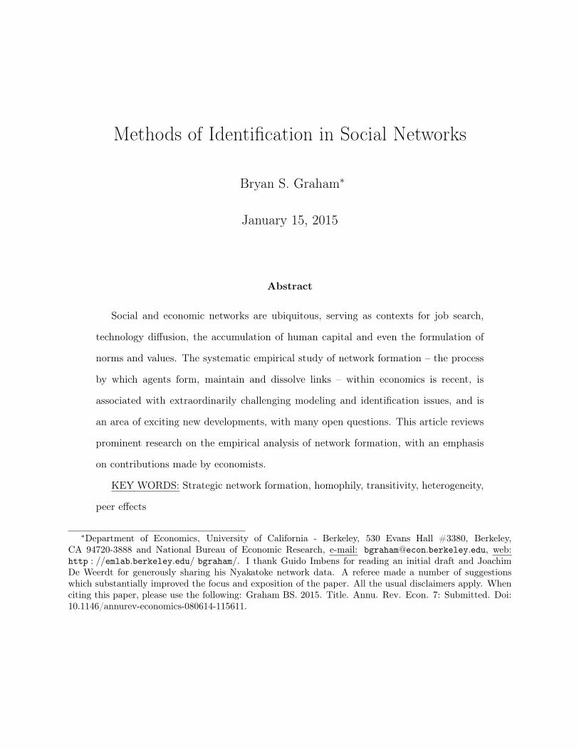
Figure 1 provides a visual representation of a set of risk-sharing links, measured in the year

2000, between 119 households residing in Nyakatoke, a small village in Tanzania. These

data are described and analyzed by de Weerdt (2004) and de Weerdt and Fafchamps (2011).

Individuals were asked for lists of people that they could “personally rely on for help”. A list

of undirected links between all households was constructed using responses to this question.

Each point in the figure represents a household, lines between points links (see the notes to

Figure 1 for an explanation of other features of the graph)

Graphical representations of network data like Figure 1 have historically played an important

role in empirical analysis and continue to do so (Freeman, 2000). While certain features of a

network can often be intuited from a visual representation, it is also valuable to have a suite

of standard network summary statistics. This section describes methods for summarizing

network data. There are many basic references for the material surveyed here, including

2

Figure 1: Nyakatoke risk-sharing network

Source: de Weerdt (2004) and author’s calculations.Notes: Node size proportional to household degree. Yellow nodes represent householdswith land and livestock wealth below 150,000 Tanzanian Shillings, orange those with wealthbetween 150,000 and 300,000 Shillings, green those with wealth between 300,000 and 600,000Shillings and blue those with wealth of 600,000 Shillings and above. Following Comola andFafchamps (forthcoming) land was valued at 300,000 shillings per acre. Network plottedusing igraph package in R (see http : //igraph.org/r/).

3

Wasserman and Faust (1994), Newman (2003), Jackson (2008) and Kolaczyk (2009). A few

minor results presented below, mostly of pedagogical significance, are new.

The mathematical language of networks is that of discrete math and, specifically, graph

theory. An undirected graph G (N , E) consists of a set of nodes N = {1, . . . , N} and a list

of unordered pairs of nodes called edges E = {{i, j} , {k, l} , . . .} for i, j, k, l ∈ N . A graph is

conveniently represented by its adjacency matrix D = [Dij] where

Dij =

1 if {i, j} ∈ E

0 otherwise. (1)

A node, depending on the context, may be called a vertex, agent or player. Likewise edges

may be called links, friendships, connections or ties. Since self-ties are ruled-out, and the

nodes in edges are unordered, the adjacency matrix is a symmetric binary matrix with a

diagonal of so-called structural zeros (i.e., Dij = Dji and Dii = 0).

Networks may also be directed, such that each link has an ego (sender) and alter (receiver)

ordering. The focus on undirected networks here is soley for pedagogical reasons.

A social network consists of a set of agents (nodes) and ties (edges) between them. A social

network can be conveniently represented by it node and edge list or by its adjacency matrix.

I will utilize the adjacency matrix representation in most of what follows. Two examples of

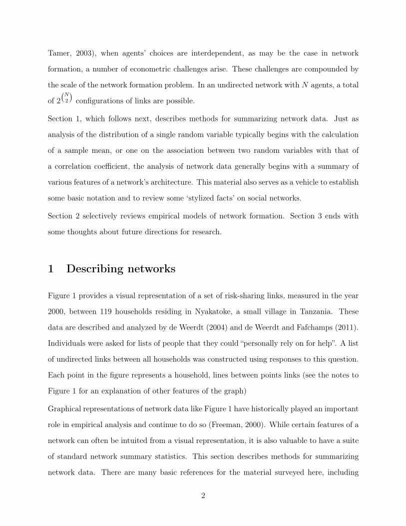
undirected network adjacency matrices are

Dex1 =

0 1 1 1 1

1 0 0 0 0

1 0 0 0 0

1 0 0 0 0

1 0 0 0 0

, Dex2 =

0 1 1 0 0

1 0 1 0 0

1 1 0 1 1

0 0 1 0 1

0 0 1 1 0

.

These two networks are graphically depicted in Figure 2. The first network, Dex1, takes a so

4

Figure 2: Two simple networks

called ‘star’ configuration, in which a central agent is linked to all other agents. The second

network, Dex2, consists of two triangles, which share a single agent in common.

In summarizing the structure of a social network it is convenient to define network statistics

at the level of individual agents, at the level of pairs of agents or dyads, and at the level of

triples of agents or triads.

Network statistics involving single agents and paths through the network

The total number of links belonging to agent i, or her degree is Di+ =∑

j Dij. The degree

frequency distribution of a network, or degree distribution for short, consists of the frequency

of each possible agent-level degree count {0, 1, . . . , N} in the network. A important com-

ponent of the literature on networks takes the degree distribution as its primitive object of

interest (e.g., Barabási and Albert (1999) and Albert and Barabási (2002)). This focus is

motivated by the fact that many other topological features of a network are fundamentally

constrained by its degree distribution (see Faust, 2007). I will have more to stay about the

connection between a network’s degree sequence and its other topological features below.

The density of a network equals the frequency with which any randomly drawn dyad is

linked:

PN =

(N

2

)−1 N∑i=1

∑j<i

Dij. (2)

5

Note that (N − 1)PN coincides with average degree. The density of the Nyakatoke network

is 0.0698. The density of Dex1 is 0.4, that of Dex2 is 0.6.

Consider the matrix product

D2 =

D1+

∑iD1iD2i · · ·

∑iD1iDNi∑

iD1iD2i D2+ · · ·∑

iD2iDNi

...... . . . ...∑

iD1iDNi

∑iD2iDNi · · · DN+

.

The ith diagonal element of D2 equals the number of agent i’s links or her degree. The

{i, j}th element of D2 gives the number of links agent i has in common with agent j (i.e.,

the number of “friends in common”). In the language of graph theory, the {i, j}th element of

D2 gives the number of paths of length two from agent i to agent j. For example, if i and j

share the common friend k, then a length two path from i to j is given by i→ k → j. The

diagonal elements of D2 correspond to the number of length two paths from an agent back

to herself. For example if i is connected to k, then one such path is i→ k → i. The number

of such paths coincides with an agent’s degree.

Calculating D3 yields a matrix whose {i, j}th element gives the number of paths of length 3

from i to j. The diagonal elements of D3 are counts of the number of transitive triads or

triangles in the network. If both i and j are connected to k as well as to each other, then

the {i, j, k} triad is closed (i.e., “the friend of my friend is also my friend”). Note that if

{i, j, k} is a closed triad it is counted twice each in the ith, jth and kth diagonal elements of

D3. Therefore Tr (D3) /6 equals the number of unique triangles in the network.

Proceeding inductively it is easy to show that the {i, j}th element of DK gives the number

of paths of length K from agent i to agent j.

6

Table 1: Frequency of degrees of separation in the Nyakatoke network1 2 3 4 5

Count 490 2666 3298 557 10Frequency 0.0698 0.3797 0.4697 0.0793 0.0014

Source: de Weerdt (2004) and author’s calculations.

Network statistics involving pairs of agents or dyads

The distance between agents i and j corresponds to the minimum length path connecting

them. If there is no path connecting i to j, then the distance between them is infinite. We

can use powers of the adjacency matrix to calculate these distances. Specifically,

Mij = mink∈{1,2,3,...}

{k : D

(k)ij > 0

}

equals the distance from i to j (if it is finite). Here D(k)ij denotes the ijth element of Dk.

If the network consists of a single, giant, connected component, such that the minimum

length path between any two agents is finite, we can compute average path length as

M =

(N

2

)−1 N∑i=1

∑j<i

Mij. (3)

If the network consists of multiple connected components, standard practice is to compute

average path length within the largest one (see Newman (2003) for an alternative measure).

The diameter of a network is the largest distance between two agents in it. It will be finite if

the network consists of a single connected component (in which case all agents are “reachable”

starting from any given agent) and infinite in networks consisting of multiple components

(in which case there are no paths connecting some pairs of agents).

Table 1 gives the frequency of minimum path lengths in the Nykatoke network. There are

490 direct ties in the network (paths of length one). Just under 7 percent of all pairs of

households are directly connected in Nykatoke. Another 2,666 dyads are only two degrees

apart. That is, although they are not connected directly, they share a tie in common. About

7

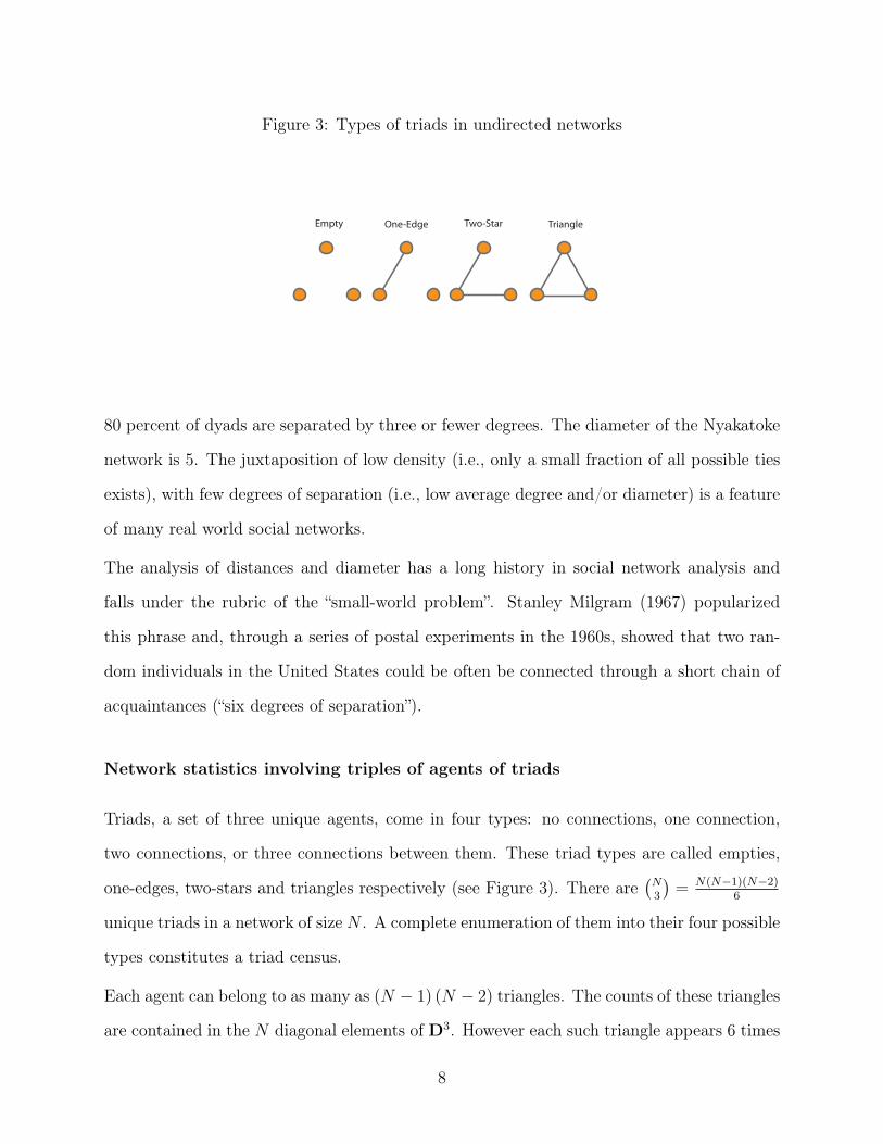
Figure 3: Types of triads in undirected networks

Empty One-Edge Two-Star Triangle

80 percent of dyads are separated by three or fewer degrees. The diameter of the Nyakatoke

network is 5. The juxtaposition of low density (i.e., only a small fraction of all possible ties

exists), with few degrees of separation (i.e., low average degree and/or diameter) is a feature

of many real world social networks.

The analysis of distances and diameter has a long history in social network analysis and

falls under the rubric of the “small-world problem”. Stanley Milgram (1967) popularized

this phrase and, through a series of postal experiments in the 1960s, showed that two ran-

dom individuals in the United States could be often be connected through a short chain of

acquaintances (“six degrees of separation”).

Network statistics involving triples of agents of triads

Triads, a set of three unique agents, come in four types: no connections, one connection,

two connections, or three connections between them. These triad types are called empties,

one-edges, two-stars and triangles respectively (see Figure 3). There are(N3

)= N(N−1)(N−2)

6

unique triads in a network of size N . A complete enumeration of them into their four possible

types constitutes a triad census.

Each agent can belong to as many as (N − 1) (N − 2) triangles. The counts of these triangles

are contained in the N diagonal elements of D3. However each such triangle appears 6 times

8

Table 2: Nyakatoke risk-sharing network triad censusempty one-edge two-star triangle

Count 221,189 48,245 4,070 315Proportion 0.8078 0.1762 0.0149 0.0012Random Graph Proportion 0.8049 0.1812 0.0136 0.0003

Source: de Weerdt (2004) and author’s calculations.Notes: The Nyakatoke network includes N = 119 households, corresponding to

(N2

)= 7, 021

unique dyads and(N3

)= 273, 819 unique triads.

in these counts: as {i, j, k}, {i, k, j}, {j, i, k}, {j, k, i}, {k, i, j} and {k, j, i}. Thus

# of triangles = TT =Tr (D3)

6(4)

equals the number of unique triangles in the network (as asserted earlier).

With a little bit of work it is possible to show that the numbers of “two-stars” and “one-edges”

can be calculated using the expressions:

# of two stars = TTS = vech(D2)′ι− Tr (D3)

2(5)

# of one edges = TOE = (N − 2) vech (D)′ ι− 2vech(D2)′ι+

Tr (D3)

2. (6)

The number of empty triads, TE, equals(N3

)minus the sum of (4), (5) and (6). We also have

the implication

TOE + 2TTS + 3TT = (N − 2) vech (D)′ ι =,1

4N (N − 1) (N − 2)PN ,

suggesting that network density can be computed from the triad census according to

PN =

(4TOE + 8TTS + 12TTN (N − 1) (N − 2)

). (7)

The triad census for the Nyakatoke network is given in Table 2. As a point of comparison

9

the proportion of each type of triad that we would expect to see in a random graph, where

the probability of a link between any two agents coincides with the observed density of the

Nyakatoke network (0.0698), is given in the last row of the table.

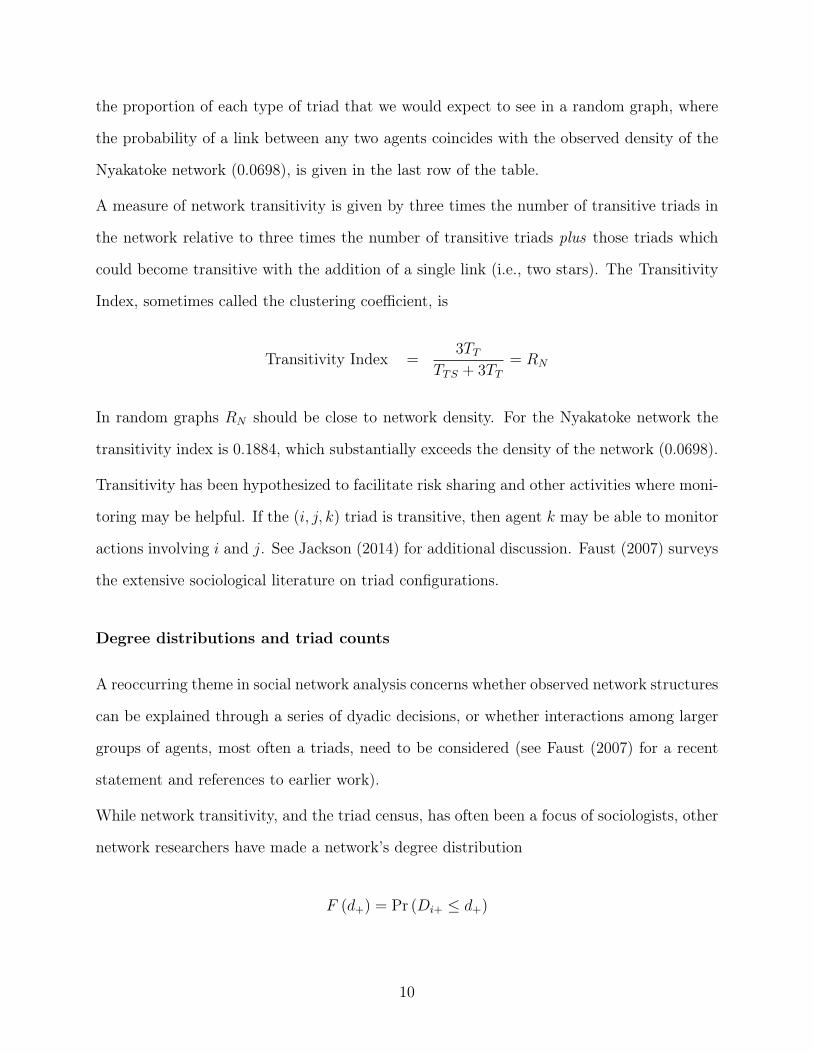
A measure of network transitivity is given by three times the number of transitive triads in

the network relative to three times the number of transitive triads plus those triads which

could become transitive with the addition of a single link (i.e., two stars). The Transitivity

Index, sometimes called the clustering coefficient, is

Transitivity Index =3TT

TTS + 3TT= RN

In random graphs RN should be close to network density. For the Nyakatoke network the

transitivity index is 0.1884, which substantially exceeds the density of the network (0.0698).

Transitivity has been hypothesized to facilitate risk sharing and other activities where moni-

toring may be helpful. If the (i, j, k) triad is transitive, then agent k may be able to monitor

actions involving i and j. See Jackson (2014) for additional discussion. Faust (2007) surveys

the extensive sociological literature on triad configurations.

Degree distributions and triad counts

A reoccurring theme in social network analysis concerns whether observed network structures

can be explained through a series of dyadic decisions, or whether interactions among larger

groups of agents, most often a triads, need to be considered (see Faust (2007) for a recent

statement and references to earlier work).

While network transitivity, and the triad census, has often been a focus of sociologists, other

network researchers have made a network’s degree distribution

F (d+) = Pr (Di+ ≤ d+)

10

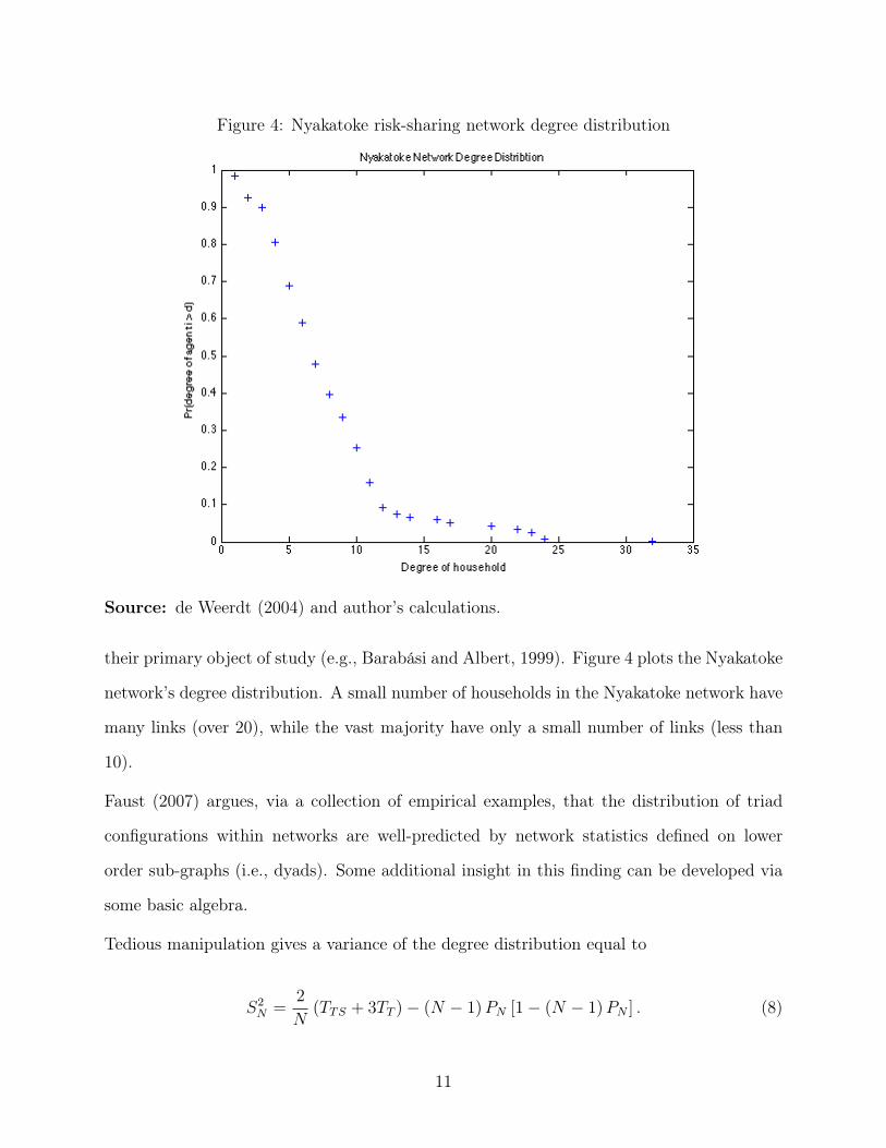
Figure 4: Nyakatoke risk-sharing network degree distribution

Source: de Weerdt (2004) and author’s calculations.

their primary object of study (e.g., Barabási and Albert, 1999). Figure 4 plots the Nyakatoke

network’s degree distribution. A small number of households in the Nyakatoke network have

many links (over 20), while the vast majority have only a small number of links (less than

10).

Faust (2007) argues, via a collection of empirical examples, that the distribution of triad

configurations within networks are well-predicted by network statistics defined on lower

order sub-graphs (i.e., dyads). Some additional insight in this finding can be developed via

some basic algebra.

Tedious manipulation gives a variance of the degree distribution equal to

S2N =

2

N(TTS + 3TT )− (N − 1)PN [1− (N − 1)PN ] . (8)

11

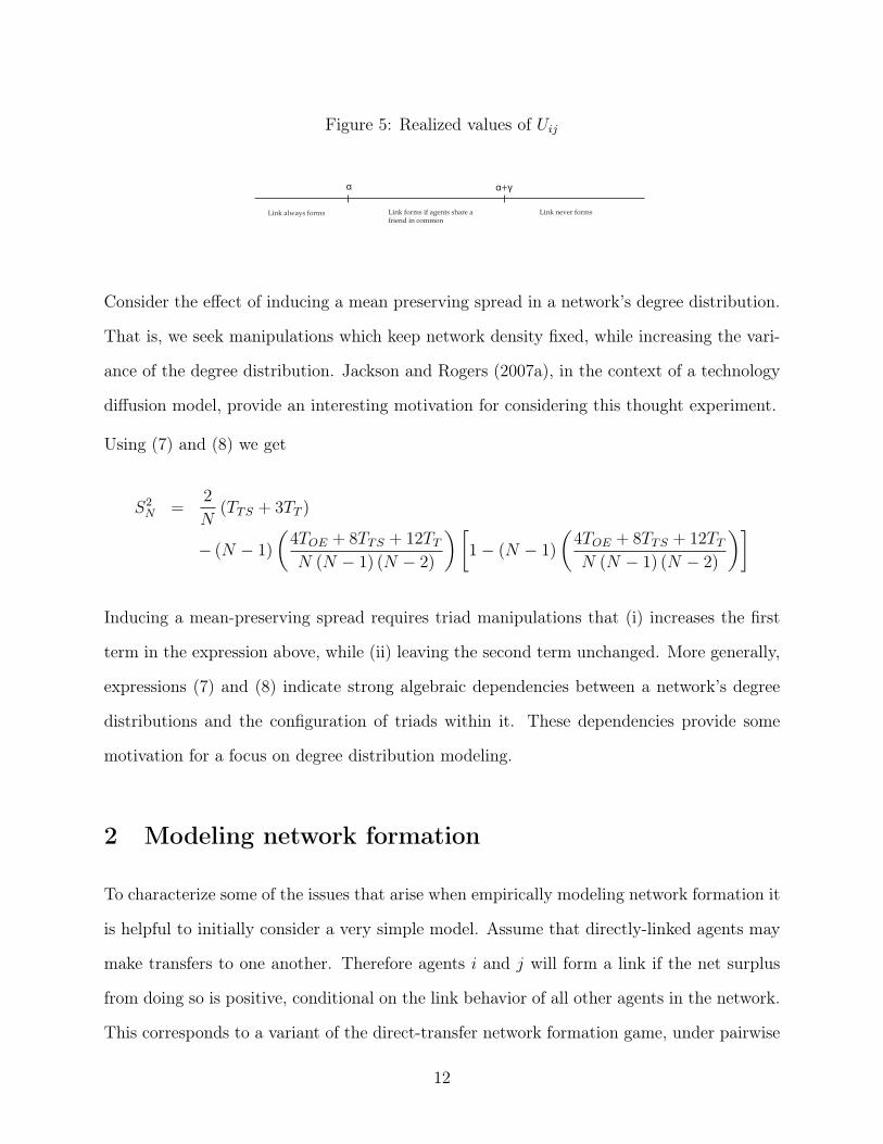
Figure 5: Realized values of Uij

α α+γ

Link always forms Link forms if agents share a friend in common

Link never forms

Consider the effect of inducing a mean preserving spread in a network’s degree distribution.

That is, we seek manipulations which keep network density fixed, while increasing the vari-

ance of the degree distribution. Jackson and Rogers (2007a), in the context of a technology

diffusion model, provide an interesting motivation for considering this thought experiment.

Using (7) and (8) we get

S2N =

2

N(TTS + 3TT )

− (N − 1)

(4TOE + 8TTS + 12TTN (N − 1) (N − 2)

)[1− (N − 1)

(4TOE + 8TTS + 12TTN (N − 1) (N − 2)

)]

Inducing a mean-preserving spread requires triad manipulations that (i) increases the first

term in the expression above, while (ii) leaving the second term unchanged. More generally,

expressions (7) and (8) indicate strong algebraic dependencies between a network’s degree

distributions and the configuration of triads within it. These dependencies provide some

motivation for a focus on degree distribution modeling.

2 Modeling network formation

To characterize some of the issues that arise when empirically modeling network formation it

is helpful to initially consider a very simple model. Assume that directly-linked agents may

make transfers to one another. Therefore agents i and j will form a link if the net surplus

from doing so is positive, conditional on the link behavior of all other agents in the network.

This corresponds to a variant of the direct-transfer network formation game, under pairwise

12

equilibrium, studied by Bloch and Jackson (2007). Let Fij (D) =(∑N

k=1DikDjk

)denote

the number of friends agents i and j share in common. Links form according to the rule

Dij = 1 (α0 + γ0Fij (D)− Uij ≥ 0) (9)

for i = 1, . . . , N and j < i. Here Uij is an unobserved component of link surplus; indepen-

dently and identically distributed across dyads according to a known distribution:

Uijiid∼ FU , i = 1, . . . , N, j < i Uij ∈ U. (10)

Rule (9) implies that agents form links if (i) they share many friends in common (Fij (D))

and/or (ii) the unobserved idiosyncratic utility from doing so is high (−Uij). The magnitude

of γ0 > 0 captures the strength of agents’ preferences for triadic closure in links. The depen-

dence of the surplus generated by an i-to-j link on the presence or absence of links across

other pairs of agents constitutes an externality. Externalities generate complex interdepen-

dencies across the choices of different agents, a modeling challenge not present in textbook

single agent models.

As noted earlier, in real world social networks linked agents often share additional links in

common, generating a clustering of ties. Rule (9) generates such clustering by positing a

structural taste for link transitivity – the returns to a relationship are higher if two individuals

share a friend in common. A preference for transitive links may be micro-founded in a variety

of ways. For example, actions between dyad partners can be monitored or refereed by a

shared friend; this may be valuable in the context of a risk-sharing network. Alternatively it

may be more enjoyable to socialize with two friends, if they are also friends with each other.

An alternative explanation for clustering is that agents assortatively match on some un-

observed attribute. Assortative matching is typically referred to as homophily in the net-

work literature. Homophily on observed attributes is a feature of many real-world networks

(McPherson, Smith-Lovin and Cook, 2001). An econometrician might reasonable worry

13

that observed patterns of link formation in a network are, in fact, driven by sorting on an

unobserved agent attribute. Rule (9) and assumption (10) rules out homophily a priori.

As an alternative to (9) Handcock, Raftery and Tantrum (2007), Krivitsky, Handcock,

Raftery and Hoff (2009) and Graham (2014), consider link formation rules like

Dij = 1(Z ′ijη0 + νi + νj − g (ξi, ξj; δ0)− Uij ≥ 0

), (11)

where Zij is an observed K × 1 vector of dyad attributes, νi and ξi are unobserved agent-

level heterogeneity, and Uij is an idiosyncratic dyad level surplus component; g (ξi, ξj; δ0) is

a known family of symmetric distance functions indexed by δ0 which (i) takes a value of zero

at ξi = ξj and (ii) is increasing in |ξi − ξj| . The goal is to learn about η0, δ0 and features of

the conditional distribution of (νi, ξi) given Z.

Relative to rule (9), rule (11) introduces a much richer form of unobserved agent-level het-

erogeneity. First, agents are heterogeneous in the amount of link surplus they generate.

Agents with high values νi generically generate more surplus. Such agents will have more

links, giving rise to degree heterogeneity; an important feature of real work networks (see

Figure 4). Second, the model allows for assortative matching on ξi. Agents which are similar

in terms of the unobserved characteristic ξi generate more surplus from linking. This feature

of the model induces clustering in links. Unlike rule (9), rule (11) does not include any

externalities: the presence or absence of a link elsewhere in the network does not change the

returns to an i-to-j link.

In practice link rules with externalities and those with rich forms of agent-level heterogene-

ity can generate very similar networks. This makes discriminating between, for example,

structural transitivity and homophily on unobservables difficult. Nevertheless, distinguish-

ing between them is scientifically interesting and policy-relevant. Transitivity is associated

with an externality in link formation. In the presence of externalities a local manipulation

of network structure can influence link formation elsewhere in the network. If clustering is

14

due soley to homophily, local manipulations do not have effects that cascade through the

network.

Below I discuss how panel data may be used to model both a structural taste for transitivity

and assortative matching on unobserved attributes simultaneously. Initially, however, I focus

on cross-sectional models that include either network externalities or heterogeneity, but not

both.

A simple cross-sectional model with structural transitivity

Returning to link rule (9), assume that the econometrician bases her inferences on a random

sample of networks from some well-defined population (of networks). For example networks

of food sharing among households across a population of indigenous communities (e.g., Koster

and Leckie, 2014). For each sampled network (community) the entire adjacency matrix

is observed. This sampling process asymptotically reveals F (D|N = n) for network size

n ∈ N = {2, 3, 4, . . .}. Implicit in (5) is the assumption that the distribution of Uij is

independent of network size. The notation Dij corresponds to the link status of the generic,

randomly drawn, (i, j) dyad, itself sampled from a randomly drawn network. To economize

on notation there is no explicit network subscript in what follows.

Equation (9) defines a system of(N2

)simultaneous discrete choices. Viewed in this way,

two questions naturally arise. First, for a given θ0 = (α0, γ0)′ does (9) have a solution for

all U ∈ UN? This is a question of equilibrium existence or model coherence. Demonstrat-

ing existence can be non-trivial for some models of network formation (cf., Jackson, 2008;

Chapter 11; Hellmann, 2013). Second, if an equilibria does exist, is it unique (again for all

U ∈ UN)? This is a question about model completeness: given a particular draw of the

model’s underlying latent variable U, does it deliver a unique prediction for the observed

network, D? Multiplicity of equilibrium network configurations is a common feature of many

models with network externalities.

The study of models with qualitative features similar to those of (9) has a long history

15

in econometrics (e.g., Heckman, 1978a). Important recent contributions include those of

Bresnahan and Reiss (1991), Tamer (2003) and Ciliberto and Tamer (2009) among others.

Unfortunately the combinatoric complexity of networks, with 2

(N2

)link configurations pos-

sible in a network with N agents, makes the direct application of insights from prior work

difficult.

To keep the discussion simple assume that N = 3. In this case there are four possible

non-isomorphic network configurations corresponding to the four types of triads depicted in

Figure 3 above. The heterogeneity draw is given by the triple U = (U12, U13, U23)′∈ U3. For

any given draw of U one of these four configurations will be observed.

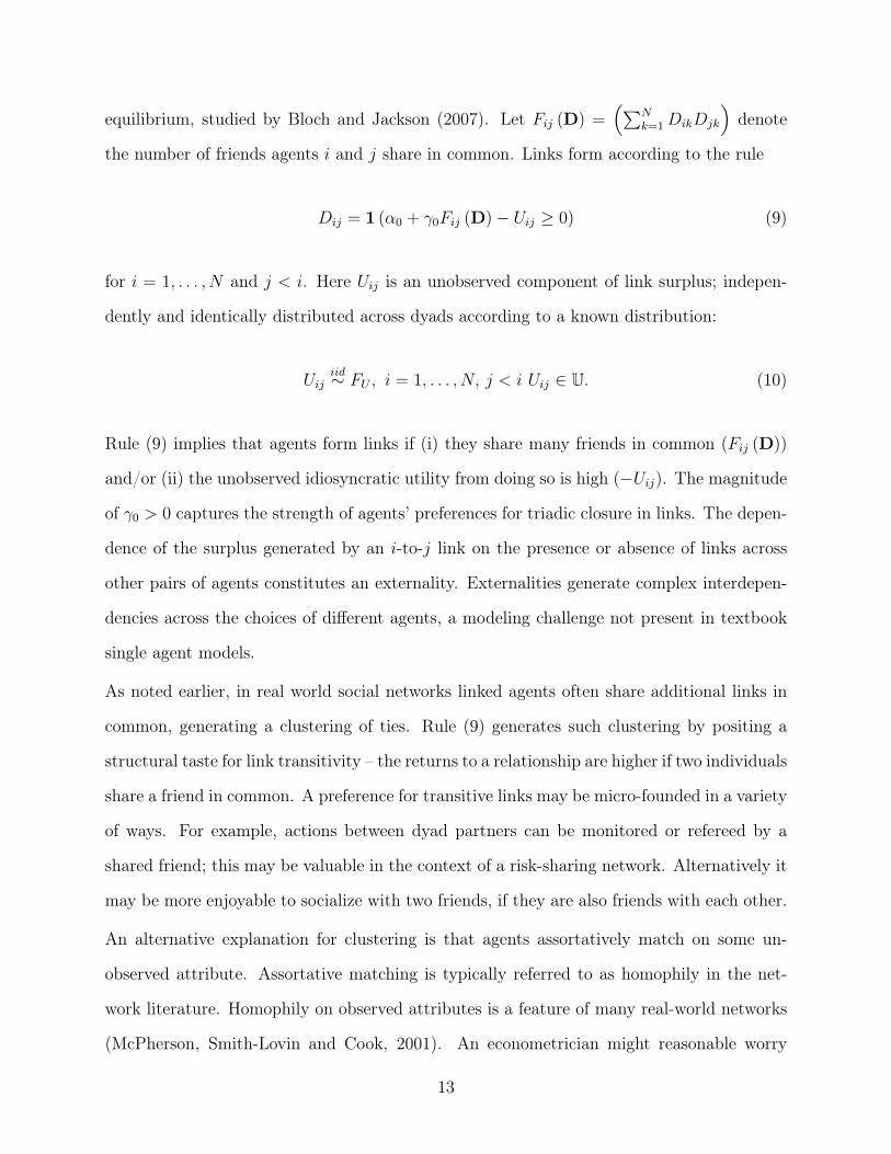
Call draws of Uij below α, between α and α+γ, and above α+γ respectively low (L), medium

(M) and high (H) draws (see Figure 5). Let pLLL (θ, FU) = FU (α)3 denote the probability of

three ‘low’ draws; pLMH (θ, FU) = FU (α)FU (α + γ) [1− FU (α + γ)] the probability of one

low, one medium and one high draw and so on. Observe that low draws of Uij correspond

to higher link surplus.

If U12 falls in the ‘low’ region, then agents 1 and 2 will form a link regardless of whether

they share a friend in common (i.e., D13D23 may equal zero or one). In contrast if U12 falls

in the ‘medium’ region, then agents 1 and 2 will form a link only if they share a friend in

common (i.e., if D13D23 = 1). If U12 falls in the ‘high’ region, then they never form a link.

The contingent behavior associated with a ‘medium’ idiosyncratic surplus component is what

generates the possibility of multiple equilibria. Consider the case where all three elements

of U fall into the ‘medium’ range. In that case two network configurations are consistent

with (9): (i) the empty triad and (ii) a triangle. The model, as specified, is silent on which

of these two networks is chosen.

Let πT (θ, FU) denote the minimum probability the model defined by (9) and (10) logically

attaches to observing a triangle for a particular θ and FU . This probability coincides with

the probability mass attached to the region of U3 where the model uniquely predicts a

triangle network. Let π̄T (θ, FU) denote the maximal probability the model logical attaches

16

to observing a triangle. This probability coincides with the probability mass attached to the

region of U3 where a triangle network is either the unique network configuration, or among

the set of multiple configurations, consistent with (9).

Recalling the notation of ‘T’ for ‘triangle’, ‘TS’ for ‘two-star’, ‘OE’ for ‘one-edge’ and ‘E’ for

‘empty’, the above logic yields the following probability bounds on the four non-isomorphic

network configurations:

πT (θ, FU) = pLLL (θ, FU) + pLLM (θ, FU)

π̄T (θ, FU) = pLLL (θ, FU) + pLLM (θ, FU) + pLMM (θ, FU) + pMMM (θ, FU)

πTS (θ, FU) = pLLH (θ, FU)

πOE (θ, FU) = pLMH (θ, FU) + pLHH (θ, FU)

π̄OE (θ, FU) = pLMM (θ, FU) + pLMH (θ, FU) + pLHH (θ, FU)

πE (θ, FU) = pMMH (θ, FU) + pMHH (θ, FU) + pHHH (θ, FU)

π̄E (θ, FU) = pMMM (θ, FU) + pMMH (θ, FU) + pMHH (θ, FU) + pHHH (θ, FU) .

Let πT denote the population frequency of triangle networks, etc. Rule (9) therefore delivers

the following inequality restrictions

πT (θ, FU) ≤ πT ≤ π̄T (θ, FU) (12)

πTS = πTS (θ, FU)

πOE (θ, FU) ≤ πOE ≤ π̄OE (θ, FU)

πE (θ, FU) ≤ πE ≤ π̄E (θ, FU) .

The model also generates the equalities

πT +πOE+πE = π̄T (θ, FU)+πOE (θ, FU)+πE (θ, FU) = πT (θ, FU)+ π̄OE (θ, FU)+ π̄E (θ, FU) .

(13)

17

The identified set, ΘI , is the set of all θ ∈ Θ such that (12) and (13) are satisfied. Ciliberto

and Tamer (2009), among others, discuss methods of estimating ΘI and conducting inference

on it and/or on θ0.

The observation that link formation rule (9) is a system of simultaneous discrete choices and,

further, that this system generates a set of moment inequalities which may be used as a basis

for inference on θ0, appears promising. Unfortunately, this observation may be of limited

practical importance (at least without invoking additional assumptions). In a network with

N agents, there are 2

(N2

)possible configurations of links. For each U in UN and θ ∈ Θ, the

consistency of a given network with (9) must be checked. In practice this is not feasible in

real time for all but very small networks. Even showing that two networks are isomorphic is

a non-trivial problem (e.g., Read and Corneil, 1977).

While fully exploiting the identifying power of (9) and (10) may be difficult in even modest-

sized networks, exploiting some of its identifying content is straightforward. Assume that

networks vary in size with N ∈ N = {2, 3, 4, . . .} and recall that the distribution of Uij is

constant in N . Under (9) and (10) the probability that a randomly drawn dyad from a

network of size N is linked (i.e., density in networks of size N) satisfies the inequalities

FU (α0) ≤ Pr (Dij = 1|N) ≤ FU (α0 + γ0 (N − 2))

for all N ∈ N. The lower bound occurs when the randomly drawn dyad share no friends

in common, the upper bound when the dyad is linked to all other members of the network

(except possibly each other).

These upper and lower bounds coincide at N = 2 so that α0 pointed identified by the density

of links across networks consisting of a single dyad:

α0 = F−1U (Pr (Dij = 1|N = 2)) .

18

A lower bound on γ0 is then given by

γ = sup

{F−1U (Pr (Dij = 1|N))− α0

N − 2

∣∣∣∣ N ∈ N}.

Here an informative lower bound on γ0 is generated by observing a higher density of link

formation in networks with N > 2, than across networks consisting of single dyads. This

does not strike me as an especially attractive approach to inferring the presence of a taste for

transitivity, but it is illustrative of how some identifying implications of a network formation

model can be easy to exploit (even if utilizing all implications is impractical).

Another, and more interesting, example of this type of approach is provided by Sheng (2012),

who explores the the identifying content of (non-trivial) subnetwork configurations. Assume

networks consist of N agents and consider the probability that, for a randomly drawn triad,

itself drawn from a randomly sampled network, we observe a particular triad configuration

(see Figure 3). This probability will depend on the degree to which members of the sampled

triad are connected to the rest of the network. Maximal connection occurs when all members

of the sampled triad are connected to all other agents in the network. Isolation occurs when

no member of the triad is linked to other agents in the network.

Now imagine repeating the thought experiment used to derive (12) above, but doing so

conditional on different assumptions about the triad’s connectivity to the rest of the network.

For example conditional on the three dyads forming the triad having, say, no, two and two

friends (outside the triad) in common, the model provides upper and lower bounds on the

probability of observing, say, a triangle configuration. An identification region for θ0 can be

computed using the union of these conditional bounds on each triad configuration (computed

for all possible degrees of triad connectivity). In a very recent working paper, de Paula,

Richards-Shubik and Tamer (2014) develop methods for computing an identification region

for θ0 based upon the frequency of various local network configurations.

Christakis, Fowler, Imbens and Kalyanaraman (2010) suggest an alternative approach to

19

dealing with the inferential challenges posed by multiplicity. They posit that the network

forms sequentially. Agents form, maintain or dissolve links in a specific order and do so

myopically. Specifically they do not anticipate how the links they choose to form today

change the incentives for link formation faced by subsequent agents.

Returning to the N = 3 case, assume that U12, U13 and U23 are respectively low, low and

medium draws (see Figure 5). Assume that agent 1 forms links first, followed by agents two

and three. Under this ordering, agent 1 will immediately form links with both agents 2 and

3. Agent 2 will then form a link with agent 3. Although the idiosyncratic utility from this

link is only ‘medium’, the link forms to reap the benefits of triadic closure, since both agents

2 and 3 already share 1 as a friend. Finally, agent 3 maintains all links formed earlier. The

triangle configuration emerges from this ordering (and draw of U).

Now consider the alternative ordering where agent 3 forms links first, followed by agents 2

and 1. In this case agent 3 will form a link with agent 1, but not 2. The absence of the

utility gain associated with triadic closure means the 2-to-3 link does not form. Agent 2 then

forms a link with 1. Finally, agent 1 maintains her links with agents 2 and 3. A two-star

configuration emerges from this ordering.

As the above examples indicate, if the ordering of link formation opportunities were ob-

served, likelihood-based inference would be straightforward. Christakis, Fowler, Imbens and

Kalyanaraman (2010) address the unobservability of the posited sequential network forma-

tion process by assigning a probability distribution to agents’ ordering, and then working

with the resulting integrated likelihood. In the the simple example discussed here, there are

N ! = 3! = 6 possible orderings. If each ordering is a priori assumed equally likely the likeli-

hood is easily written down. Christakis, Fowler, Imbens and Kalyanaraman (2010) approach

to inference is Bayesian (and based on the observation of a single network). An important

contribution of their paper is to make the simple idea sketched above computationally op-

erational for realistically-sized networks. Specifically, they use Markov Chain Monte Carlo

(MCMC) methods to take draws from a posterior distribution for the model parameters.

20

An potentially unattractive feature of assuming the network is formed sequentially, is that

the resulting likelihood will, for certain values of U, place positive probability on network

configurations that do not correspond to an equilibrium of the simultaneous-move static

game. This is again illustrated by the example above. In the static game a low, low, medium

draw of U uniquely predicts a triangle network. For the same draw of U the sequential game

places a probability of two-thirds on the triangle network, and a probability of one-third on

the two-star network. If, in reality, agents have the opportunity to continually revise their

links, a two-star configuration would not emerge conditional on a low, low and medium draw

of idiosyncratic link surpluses. Of course, in some settings, it might be very reasonable to

assume links form sequentially and irreversibly. Similarly considerations arise when deciding

whether to model firm interactions with a Stackelberg leadership model or a simultaneous

move game.

Mele (2013) develops a related approach to empirically modeling network formation. He

posits a process whereby in each ‘period’ a randomly drawn dyad is given the opportunity

to form, maintain or dissolve a link. For a specific specification of link surplus and meeting

probabilities, he shows that the sequence of networks generated by the model is a stationary

ergodic process. The long-run probabilities attached to specific network configurations are

used to formulate a likelihood. Like, Christakis, Fowler, Imbens and Kalyanaraman (2010),

Mele’s (2013) approach to inference is Bayesian. He develops an MCMC algorithm for

generating draws from a posterior distribution for the model parameters. His approach

also places positivity probability on network configurations that are not equilibria of the

corresponding simultaneous-move static game.

The Sheng (2012), Christakis, Fowler, Imbens and Kalyanaraman (2010) and Mele (2013)

papers all provide operational methods for inferring the distribution of link surplus from

observed network structure. Sheng’s (2012) approach provides a computationally feasible

(albeit difficult) way to harness the identifying content of pairwise stability (see also de

Paula, Richards-Shubik and Tamer, 2014). Her approach to inference requires the observa-

21

tion of many independent networks (see also Miyaichi, 2013). Christakis, Fowler, Imbens

and Kalyanaraman (2010) and Mele (2013) show the identifying power of moving from a si-

multaneous to sequential network formation process. All three methods are computationally

intensive.

A simple cross-sectional model with heterogeneity

Now return to the link formation rule (11). This model has a rich heterogeneity structure,

complicating its analysis relative to rule (9). However rule (11) also excludes externalities in

link formation a priori, side-stepping the coherence and completeness issues associated with

rule (9).

Graham (2014) studies (11) with g (ξi, ξj; δ0) empty; that is a model with unobserved degree

heterogeneity, but no homophily on unobservables. He derives the joint maximum likelihood

estimator where both the common parameter η0 and the incidental parameters {νi}∞i=1 are

estimated simultaneously. He further assume Ui is a logistic random variable. Graham (2014)

derives the limiting distribution of the common parameter as the network grows large. This

limit distribution is normal, but includes a bias term.

Graham also proposes an estimator which conditions on a sufficient statistic for the degree

heterogeneity parameters. Charbonneau (2014), in independent work, develops a related

procedure in the context of studying gravity trade models. Random effects estimation of

(11) is pursued in Krivitsky, Handcock, Raftery and Hoff (2009) using MCMC methods.

One advantage of a fixed effects treatment of degree heterogeneity is that the resulting model

of tie formation will be able to perfectly match any observed degree sequence (cf., Chatter-

jee, Diaconis and Sly, 2011). As argued above algebraically, and shown by Faust (2007)

empirically, a network’s degree distribution often does a reasonably good job of explaining

(i.e., predicting) other “higher order” aspects of network architecture (e.g., the frequency of

different triad configurations). For this reason analyses based on (11) are likely to provide

good fits, even if the true link formation process includes interdependent preferences.

22

Dynamic models of network formation

If the econometrician observes the structure of links within a network evolve over time, a

number of new modeling opportunities arise. In particular is becomes possible to meaningful

incorporate both interdependent preferences and rich forms of agent level heterogeneity into

a single model of link formation. Let t = 0, 1, 2, 3 index the periods in which each network

is observed and assume that links form in period t according to the rule

Dijt = 1 (β0Dijt−1 + γ0Fijt−t (Dt−1) + Aij − Uij ≥ 0) (14)

with, for example,

Aij = νi + νj − g (ξi, ξj) , (15)

where all notation is as previously defined. Model (14) combines features of the two static

models discussed above (rules (9) and (11)). It incorporates key network dependencies

emphasized in prior work (cf., Snijders, 2011). First, links are persistent. If agents i and

j are linked in period t, they are more likely to be linked in subsequent periods (β0 > 0).

Second, as in the first static model discussed above, there are returns to ‘triadic closure’

(γ0 > 0). The net surplus associated with an i-to-j link is increasing in the number of

friends i and j shared in common during the prior period. Third and fourth, as in the

second static model discussed above, both degree heterogeneity and assortative matching on

unobservables are incorporated.

As in Christakis, Fowler, Imbens and Kalyanaraman (2010) and Mele (2013), model (14)

implies that agents form links myopically. At the beginning of each period agents form,

maintain and dissolve thinks ‘as if’ all other features of the network will remain fixed. This

is analogous to a best-reply dynamic. Assuming a best-reply type dynamic eliminates the

contemporaneous feedback which generated multiple equilibria, and its associated inferential

challenges, in the static model discussed above. At the same time, by allowing link surplus

to vary with the structure of the network in the prior period, network dependencies, such as

23

a taste for triadic closure, are incorporated into (14).

Most theoretical models of network formation assume agents form links according to some

variant of naive best-reply dynamics (e.g., Jackson and Wolinsky, 1996; Jackson and Watts,

2002; Bala and Goyal, 2000; Watts, 2001; Jackson and Rogers, 2007b), although some

scholars have studied models with forward-looking agents (e.g., Dutta, Ghosal and Ray,

2005). The dynamics of link formation implied by (14) are closely aligned with the types

of dynamics assumed by theorists. Although the myopic nature of link formation may not

be of particular concern, a more mundane, but nevertheless important, concern may arise

in empirical work. It may be that the frequency at which the network is sampled, and the

structure of links recorded, does not correspond naturally with the timing at which agents

actually make link decisions. Similar concerns arise in single agent discrete choice analyses

(cf., Chamberlain, 1985). When formulating a social network data collection protocol, the

timing of link decisions and the timing of data collection should be aligned.

In the first static model discussed above, the clustering of ties was explained soley by a taste

for triadic closure. In practice tie clustering might also arise because agents assortatively

match on attributes unobserved by the econometrician (homophily), as was assumed in the

second model. The dynamic model introduced here allows for both sources of clustering.

Goldsmith-Pinkham and Imbens (2013) take random-effects approach to model (14). If the

density of Uij is known (e.g., Standard Normal or Logistic), and the joint distribution of

(D0,A) belongs to a parametric family, then inferences on θ0 = (β0, γ0)′ may be based

on an integrated or random effects likelihood. In principle this is very much analogous to

random effects approaches to single-agent dynamic panel data models (Heckman, 1981a-c;

Chamberlain, 1985). In reality both the specification and maximization of an integrated

likelihood in this setting is non-trivial.

Ideally the specified joint distribution for (D0,A) should allow for dependence between D0

and A. Since the model implies that D1 varies with A, it seems ‘natural’ to allow the initial

network configuration, D0, to also vary with A. This is a complicated version of the initial

24

conditions problem which arises in single-agent dynamic panel data models (Wooldridge,

2005).

To get a sense of the modeling issues involved, assume that Aij takes the form given in (15)

with (νi, ξi) bivariate normal with an unknown location vector and scale matrix. Assume

that g (·, ·) is a known function, that Uijt is a standard normal random variable, and that

Dij0 = 1 (Aij − Uij0 ≥ 0) . These assumptions are sufficient to write down the integrated-

likelihood. Evaluating that likelihood, however, would be very challenging. Doing so would

involve calculating a 2N -dimensional integral. This integral does not obviously factor into

a set of lower dimensional integrals (since Aij and Akl will share components in common

whenever i = k or j = l).

Motivated by these computational challenges Goldsmith-Pinkham and Imbens (2013) instead

work with a highly stylized model. They rule out degree heterogeneity, set g (ξi, ξj) =

|ξi − ξj|, and assume that ξi is binary-valued with Pr (ξi = αξ|D0) = Pr (ξi = 0|D0) = 12.

Note that this last assumption assumes, unattractively, independence between D0 and A.

Under these assumptions Goldsmith-Pinkham and Imbens (2013) develop an algorithm for

taking draws from the posterior distribution for the model’s parameters.

Graham (2013) approaches model (14) from a fixed effects perspective, asking if it contains

implications that are invariant to A, but useful for identifying θ0. This approach leaves

the distribution of (D0,A) unspecified and unrestricted. Perhaps surprisingly, fixed effects

identification results can be derived.

Consider a dyad that is embedded in a stable neighborhood. A stable neighborhood has

two features. First, with the exception of possible link formation and dissolution between

themselves, the set of links maintained by agents i and j is the same across periods 1, 2 and

3. Agents i and j may add, maintain or delete links between periods 0 and 1. Second, the

links maintained by friends of players i and j do not change between periods 1 and 2. Dyads

in stable neighborhoods are embedded in local networks with link structures that are largely

fixed up to two degrees away across periods 1, 2, and 3.

25

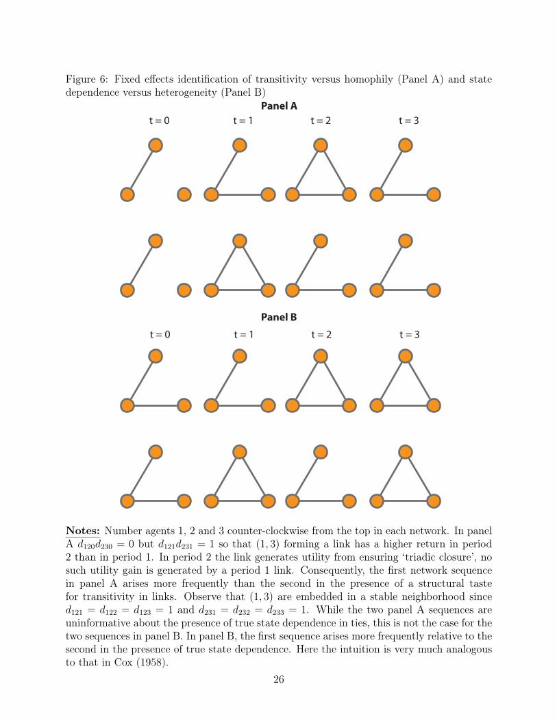
Figure 6: Fixed effects identification of transitivity versus homophily (Panel A) and statedependence versus heterogeneity (Panel B)

t = 0 t = 1 t = 2 t = 3

t = 0 t = 1 t = 2 t = 3

Panel A

Panel B

Notes: Number agents 1, 2 and 3 counter-clockwise from the top in each network. In panelA d120d230 = 0 but d121d231 = 1 so that (1, 3) forming a link has a higher return in period2 than in period 1. In period 2 the link generates utility from ensuring ‘triadic closure’, nosuch utility gain is generated by a period 1 link. Consequently, the first network sequencein panel A arises more frequently than the second in the presence of a structural tastefor transitivity in links. Observe that (1, 3) are embedded in a stable neighborhood sinced121 = d122 = d123 = 1 and d231 = d232 = d233 = 1. While the two panel A sequences areuninformative about the presence of true state dependence in ties, this is not the case for thetwo sequences in panel B. In panel B, the first sequence arises more frequently relative to thesecond in the presence of true state dependence. Here the intuition is very much analogousto that in Cox (1958).

26

Panel A of Figure 6 visually depicts two network sequences in a network consisting of three

agents. Number agents 1, 2 and 3 counter-clockwise from the top in each network. Observe

that Agents 1 and 3 are embedded in a stable neighborhood. Agent 1 is linked to agent 2,

and agent 3 to agent 2, in periods 1, 2 and 3 in both sequences depicted in Panel A.

The only difference between the two network sequences is that in the upper one agents 1 and

3 are linked in period 2, but not in period 1; while in the lower sequence they are linked in

period 1, but not in period 2. In the presence of a taste for triadic closure the net surplus

associated with a 1-to-3 link will be, in expectation, higher in period 2 than it is in period

1. Since agents 1 and 3 share a common friend in period 1, a 1-to-3 link in the next period

will generate additional utility from ensuring triadic closure. Agents 1 and 3 do not share a

common friend in period 0. Therefore forming a link in period 1 generates no extra utility

from ensuring triadic closure. In the presence of a genuine taste for transitivity in links, as

embodied in link rule (14), the upper sequence should be observed more frequently than the

lower sequence.

Panel B of Figure 6 presents an example of how the relative frequency of different sequences

of dyad links, when embedded in a different stable neighborhood from the one depicted in

Panel A, provides information about β0 or state-dependence in links.

In single agent models, fixed effects identification of true state dependence in the presence of

unobserved heterogeneity is based on the frequency of observing certain sequences of choices

relative to other sequences (e.g., Cox, 1958; Heckman, 1978b; Chamberlain, 1985; Honoré

and Kyriazidou, 2000). For example, in the absence of state dependence the binary sequences

0101 and 0011 are equally likely. In the presence of state dependence, the relative frequency

of the latter sequence will be greater.

The identification of transitivity versus homophily involves a similar intuition. Conditional

on a dyad being embedded in a certain type of local network architecture, certain order-

ings of link histories should be more frequent than others. This approach involves making

comparisons ‘holding other features of the network fixed’. This is not straightforward to do.

27

The likelihood associated with a single network sequence includes 3 × 12N (N − 1) distinct

components plus the initial condition (itself ‘high dimensional’). The challenge is that the

likelihood functions associated with the two network histories, even though they are identical

in all respects except that the (i, j) friendship history in one is a permutation of that in the

other, may be very different. This is because the presence or absence of a link in a given

period can affect the likelihood contribution of many other pairs in subsequent periods.

For example if (i, k) are linked in period t, then the addition of an (i, j) link increases the

probability of a (j, k) link in period t+ 1. Local changes in the network can have widespread

effects on the structure of the network likelihood in subsequent periods.

If (i, j) are embedded in a stable neighborhood, the two likelihoods will be nominally quite

different, however many contributions in the first likelihood will be permutations of contri-

butions which also appear in the second. As a result, the number of distinct terms in the two

likelihoods is small. Exploiting this simplification then allows for the application of identifi-

cation ideas used in prior work on binary choice (e.g., Manski, 1987; Honoré and Kyriazidou,

2000). Graham (2012), extending earlier work published in Graham (2013), show this type

of intuition can be made rigorous.

The relative strengths and weakness of fixed versus correlated random effects approaches to

dynamic network analysis, closely mirror those in single agent dynamic discrete choice anal-

ysis (cf., Chamberlain, 1984). The computational complexity of these approaches when ap-

plied to network models substantially exceeds their single-agent counterparts. The Goldsmith-

Pinkham and Imbens (2013) paper provides a valuable template for undertaking a correlated

random effects analysis. While some of their modeling assumptions are unattractive, it is

one the few coherent likelihood-based empirical models of dynamic network formation and

will no doubt be the building block for future research. The fixed-effects results in Graham

(2012, 2013) indicate that some features of the distribution of link surplus may be identified

without making assumptions about the initial network condition and/or the distribution

of unobserved dyad-level heterogeneity. A fixed effects analysis can provide evidence of a

28

structural taste for transitivity under weak assumptions and/or be used to validate specific

correlated random effects specifications.

3 Future research directions

The analysis of networks has always been a multi-disciplinary endeavor. Economists are

relative latecomers to this project. This survey has been deliberately eclectic and biased

toward recent work done by economists. This work has not been undertaken in a vac-

uum. Economists interested in studying networks would be well-advised to read widely.

Goldenberg, Zheng, Fienberg and Airoldi (2009) provide a monograph-length review of the

literature from the perspective of statistics and machine learning. Snijders (2011) surveys

the quantitative sociology literature.

At the same time there is tremendous latitude to approach network data from first princi-

ples. In my view there is not one obvious “correct” way to formulate a network formation

model (although I do privilege approaches with clear random utility foundations). At this

stage it seems apparent that a sizable component of empirical research on networks will be

computationally complex. Ideas from discrete math, computer science, and Bayesian MCMC

estimation have all proved to be very useful in work done thus far (e.g., Blitzstein and Diaco-

nis, 2011). While economists’ contributions to “network science” will be necessarily shaped

by our disciplines’ unique approaches to modeling and analyzing data, it is also the case that

there are tremendous gains from trade to sharing knowledge and know how across fields.

In thinking about identification, ideas from the recent literature on games, as well as the

more established literature on dynamic panel data, have led to valuable insights. In both

cases the combinatoric complexity of networks precludes a direct application of methods from

these literatures in all but the very simplest of cases. At the same time clever exploitation of

various peculiarities and symmetries in the network formation problem can lead to tractable

procedures.

29

This survey has not emphasized special purpose models (e.g., Currarini, Jackson and Pin,

2010). In some settings, for example those often encountered in industrial organization,

substantial additional information may be available about the form of agents’ objective

functions, the timing of decisions and so on. Building empirical models that fully exploit

all this extra information can be fruitful, both for expanding subject area knowledge and

for methodological advancement. Indeed an important component of research by economists

should involve modeling real-world datasets coherently, even if realistic models are only

aspirational at the present time.

30

References

[1] Albert, Reka and Albert-Lászlo Barabási. (2002). “Statistical mechanics of complex

networks,” Review of Modern Physics 74 (1): 47 - 97.

[2] Bala, Venkatesh and Sanjeev Goyal. (2000). “A noncooperative model of network for-

mation,” Econometrica 68 (5): 1181 - 1229.

[3] Banerjee, Abhijit, Arun G. Chandrasekhar, Esther Duflo, Matthew O. Jackson. (2013).

“The diffusion of microfinance,” Science 341 (6144 ): 363 - 370.

[4] Barabási, Albert-László and Réka Albert. (1999). “Emergence of scaling in random

networks,” Science 286 (5439): 509 - 512.

[5] Blitzstein, Joseph and Persi Diaconis. (2011). “A sequential importance sampling algo-

rithm for generating random graphs with prescribed degrees,” Internet Mathematics 6

(4): 489 - 522.

[6] Bloch, Francis and Matthew O. Jackson. (2007). “The formation of networks with trans-

fers among players,” Journal of Economic Theory 113 (1): 83 -110.

[7] Blume, Lawrence E., William A. Block, Steven N. Durlauf and Yannis M. Ioannides.

(2011). “Identification of social interactions,” Handbook of Social Economics 1B: 853 -

964 (J. Benhabib, A. Bisin, & M. Jackson, Eds.). Amsterdam: North-Holland.

[8] Bresnahan, Timothy F. and Peter C. Reiss. (1991). “Empirical models of discrete games,”

Journal of Econometrics 48 (1-2): 57 - 81.

[9] Case, Anne C. and Lawrence F. Katz. (1991). “The company you keep: the effects of

family and neighborhood on disadvantaged youths,” NBER Working Paper No. 3705.

[10] Chamberlain, Gary. (1984). “Panel data,” Handbook of Econometrics 2: 1247 - 1318 (Z.

Griliches & M. D. Intriligator, Eds.). Amsterdam: North-Holland.

31

[11] Chamberlain, Gary. (1985). “Heterogeneity, omitted variable bias, and duration depen-

dence,” Longitudinal Analysis of Labor Market Data: 3 - 38 (J.J. Heckman & B. Singer,

Eds.). Cambridge: Cambridge University Press.

[12] Charbonneau, Karyne B. (2014). “Multiple fixed effects in binary response panel data

models,” Bank of Canada Working Paper 2014-17.

[13] Chatterjee, Sourav, Persi Diaconis and Allan Sly. (2011). “Random graphs with a given

degree sequence,” Annals of Applied Probability 21 (4): 1400 - 1435.

[14] Christakis, Nicholas A., James H. Fowler, Guido W. Imbens, Karthik Kalyanaraman.

(2010). “An empirical model of strategic network formation,” NBER Working Paper No.

16039.

[15] Ciliberto, Federico and Elie Tamer. (2009). “Market structure and multiple equilibria in

airline markets,” Econometrica 77 (6): 1791 - 1828.

[16] Comola, Marghertia and Marcel Fafchamps. (forthcoming). “Testing unilateral and bi-

lateral link formation,” Economic Journal.

[17] Cox, D. R. (1958). “The regression analysis of binary sequences,” Journal of the Royal

Statistical Society B 20 (2): 215 - 241.

[18] Currarini, Sergio, Matthew O. Jackson and Paolo Pin. (2010). “Identifying the roles of

race-based choice and chance in high school friendship network formation,” Proceedings

of the National Academy of Sciences 107 (11): 4857 - 4861.

[19] de Paula, Aureo, Seth Richards-Shubik and Elie Tamer. (2014). “Identification of pref-

erences in network formation games,” Mimeo, Carnegie Mellon University.

[20] De Weerdt, Joachim. (2004). “Risk-sharing and endogenous network formation,” In-

surance Against Poverty : 197 - 216 (Dercon, Stefan, Ed.). Oxford: Oxford University

Press.

32

[21] De Weerdt, Joachim and Marcel Fafchamps. (2011). “Social identity and the formation

of health insurance networks,” Journal of Development Studies 47 (8): 1152 - 1177.

[22] Dutta, Bhaskar, Sayantan Ghosal and Debraj Ray. (2005). “Farsighted network forma-

tion,” Journal of Economic Theory 122 (2): 143 - 164.

[23] Faust, Katherine. (2007). “Very local structure in social networks,” Sociological Method-

ology 37 (1): 209 - 256.

[24] Freeman, Linton. (2000). “Visualizing social networks,” Journal of Social Structure 1

(1).

[25] Gaviria, Alejandro and Steven Raphael. (2001). “School-based peer effects and juvenile

behavior,” Review of Economics and Statistics 83 (2): 257 - 268.

[26] Goldenberg, Anna, Alice X. Zheng, Stephen E. Fienberg and Edoardo M. Airoldi.

(2009). “A survey of statistical network models,” Foundations and Trends in Machine

Learning 2 (2): 129 - 233.

[27] Goldsmith-Pinkham, Paul and Guido W. Imbens. (2013). “Social networks and the

identification of peer effects,” Journal of Business and Economic Statistics 31 (3): 253

- 264.

[28] Graham, Bryan S. (2012). “Homophily and transitivity in dynamic network formation,”

In Progress, UC - Berkeley.

[29] Graham, Bryan S. (2013). "Comment on "Social networks and the identification of peer

effects" by Paul Goldsmith-Pinkham and Guido W. Imbens," Journal of Business and

Economic Statistics 31 (3): 266 - 270, 2013.

[30] Graham, Bryan S. (2014). “An empirical model of network formation: detecting ho-

mophily when agents are heterogenous,” NBER Working Paper w20341.

33

[31] Handcock, Mark S., Adrian Raftery and Jeremy M. Tantrum. (2007). “Model-based

clustering for social networks,” Journal of the Royal Statistical Society A 170 (2): 301 -

354.

[32] Heckman, James J. (1978a). “Dummy endogenous variables in a simultaneous equation

system,” Econometrica 46 (4): 931 - 959.

[33] Heckman, James. J. (1978b). “Simple statistical models for discrete panel data developed

and applied to test the hypothesis of true state dependence against the hypothesis of

spurious state dependence,” Annales de l’inséé 30-31: 227 - 270.

[34] Heckman, James. J. (1981a) “Heterogeneity and state dependence,” Studies in Labor

Markets : 91 - 139 (S. Rosen, Ed.). Chicago: University of Chicago Press.

[35] Heckman, James. J. (1981b). “Statistical models for discrete panel data,” Structural

Analysis of Discrete Data and Econometric Applications : 114 - 178 (C.F. Manski &

D.L. McFadden, Eds.). Cambridge, MA: The MIT Press.

[36] Heckman, James. J. (1981c). “The incidental parameters problem and the problem of

initial conditions in estimating a discrete time-discrete data stochastic process,” Struc-

tural Analysis of Discrete Data and Econometric Applications : 179 - 195 (C.F. Manski

& D.L. McFadden, Eds.). Cambridge, MA: The MIT Press.

[37] Hellmann, Tim. (2013). “On the existence and uniqueness of pairwise stable networks,”

International Journal of Game Theory 42 (1): 2111 - 237.

[38] Honoré, Bo E. and Ekaterini Kyriazidou. (2000). “Panel data discrete choice models

with lagged dependent variables,” Econometrica 68 (4): 839 - 874.

[39] Jackson, Matthew O. (2008). Social and Economic Networks. Princeton, NJ: Princeton

University Press.

34

[40] Jackson, Matthew O. (2014). “Networks and the identification of economic behaviors,”

Mimeo, Stanford University.

[41] Jackson, Matthew O. and Brian W. Rogers. (2007a). “Relating network structure to dif-

fusion properties through stochastic dominance,” B.E. Journal of Theoretical Economics

7 (1) (Advances), Article 6.

[42] Jackson, Matthew O. and Brian W. Rogers. (2007b). “Meeting strangers and friends of

friends: how random are social networks?” American Economic Review 97 (3): 890 -

915.

[43] Jackson, Matthew O. and Alison Watts. (2002). “The evolution of social and economic

networks,” Journal of Economic Theory 106 (2): 265 - 295.

[44] Jackson, Matthew O. and Asher Wolinsky. (1996). “A strategic model of social and

economic networks,” Journal of Economic Theory 71 (1): 44 - 74.

[45] Kolaczyk, Eric D. (2009). Statistical Analysis of Network Data. New York: Springer.

[46] Koster, Jeremy M. and George Leckie. (2014). “Food sharing networks in lowland

Nicaragua: an application of the social relations model to count data,” Social Networks

38: 100 - 110.

[47] Kranton, Rachel E. and Deborah F. Minehart. (2001). “A theory of buyer-seller net-

works,” American Economic Review 91 (3): 485 - 508.

[48] Krivitsky, Pavel N., Mark S. Handcock, Adrian E. Raftery, and Peter D. Hoff. (2009).

“Representing degree distributions, clustering, and homophily in social networks with

latent cluster random effects models,” Social Networks 31 (3): 204 - 213.

[49] Loury, Linda Datcher. (2006). “Some contacts are more equal than others: informal

networks, job tenure, and wages,” Journal of Labor Economics 24 (2): 299 - 318.

35

[50] Manski, Charles F. (1975). “Maximum score estimation of the stochastic utility model

of choice," Journal of Econometrics 3 (3): 205 - 228.

[51] Manski, Charles F. (1987). “Semiparametric analysis of random effects linear models

from binary panel data,” Econometrica 55 (2): 357 - 362.

[52] McFadden, Daniel L. (1973). “Conditional logit analysis of qualitative choice behavior,”

Frontiers in Econometrics : 105 - 142 (P. Zarembka, Ed.). New York: Academic Press.

[53] McPherson, Miller, Lynn Smith-Lovin and James M. Cook. (2001). “Birds of a feather:

homophily in social networks,” Annual Review of Sociology 27 (1): 415 - 444.

[54] Mele, Angelo. (2011). “A structural model of segregation in social networks,” Mimeo,

John Hopkins University.

[55] Milgram, Stanley (1967). “The small-world problem,” Psychology Today 1 (1): 61 - 67.

[56] Miyaichi, Yuhei. (2013). “Structural estimation of a pairwise stable network with non-

negative externality.” Mimeo, Massachusetts Institute of Technology.

[57] Newman, Mark. E. J. (2003). “The structure and function of complex networks,” SIAM

Review 45 (2): 167 - 256.

[58] Read, Ronald C. and Corneil, Derek. G. (1977). “The graph isomorphism disease,”

Journal of Graph Theory 1 (4): 339 – 363.

[59] Sheng, Shuyang. (2012). “Identification and estimation of network formation games,”

Mimeo, University of Southern California.

[60] Snijders, Tom A.B. (2011). “Statistical models for social networks,” Annual Review of

Sociology 37 (1): 131 - 153.

[61] Tamer, Elie. (2003). “Incomplete simultaneous discrete response model with multiple

equilibria,” Review of Economic Studies 70 (1): 147 - 167.

36

[62] Wasserman, Stanley and Katherine Faust. (1994). Social Network Analysis. Cambridge:

Cambridge University Press.

[63] Watts, Alison. (2001). “A dynamic model of network formation,” Games and Economic

Behavior 34 (2): 331 - 341.

[64] Wooldridge, Jeffrey M. (2005). “Simple solutions to the initial conditions problem in dy-

namic, nonlinear panel data models with unobserved heterogeneity,” Journal of Applied

Econometrics 20 (1): 39 – 5.

37