Embed Size (px)
Citation preview
UNIVERSITÀ DEGLI STUDI DI PADOVADIPARTIMENTO DI INGEGNERIA INDUSTRIALE CORSO DI LAUREA
MAGISTRALE IN INGEGNERIA ELETTRICA
Tesi di Laurea Magistrale in Ingegneria Elettrica
METODI DI CALCOLO DEI FLUSSI DI POTENZAIN RETI RADIALI DISSIMMETRICHE
-POWER FLOW CALCULATION METHODS FOR
ASYMMETRICAL RADIAL NETWORKS
Relatore: Prof. Roberto Turri
Laureanda: FIAMMETTA CAVALLIN
ANNO ACCADEMICO 2013 – 2014

2

Abstract
In some applications like power quality and safety analyses, it is of special interest to
ascertain the power flow in the network. This is an issue that has become more
important with the increasing of the distributed generation.
In this work a problem with a three-phase distribution network is analysed. Using the
tool MATLAB, the radial network under analysis has been represented and studied.
A system comprising 10 mini-pillars and 74 customers has been developed. Both the
neutral wire and ground were included.
This work has the objective of recognising flaws and strengths of some approaches
to the power flow calculation methods. Here reported are the results of what I could
first learn, during a three months experience I made at the Dublin Institute of
Technology in Ireland, and then more deeply analysed, once came back at the
Department of Industrial Engineering of Padova in Italy.
3

4

Index
INTRODUCTION.......................................................................................................9
CHAPTER 1 − Introduction to Smart Grids...........................................................111.1 DISTRIBUTED ENERGY SUPPLY..................................................................................11
CHAPTER 2 − Dublin, Ireland...............................................................................13 2.1 MY WORK IN DUBLIN...............................................................................................143.1.1 About the considered network.......................................................................................14
CHAPTER 3 − The Backward - Forward Method................................................173.1 HOW IT WORKS.......................................................................................................173.2 REPRESENTATION OF THE NETWORK..............................................................................193.3 CARSON-CLEM’S EQUATIONS...................................................................................233.4 REPRESENTATION OF THE GENERATORS...................................................................303.5 REPRESENTATION OF THE LOADS.............................................................................303.6 DIFFERENT IMPLEMENTATIONS................................................................................313.6.1 Ciric’s scheme...............................................................................................................313.6.2 With Carson-Clem’s equations......................................................................................323.7 WHICH IS THE ACTUAL ISSUE..................................................................................34
CHAPTER 4 − Analysis of the network structure................................................37 4.1 THE ALGORITHM STRUCTURE ....................................................................................374.1.1 Model_entire_network..................................................................................................384.1.2 Sys_Load.......................................................................................................................384.1.3 Branch_Current.............................................................................................................394.1.4 Pillar_Current................................................................................................................394.1.5 Voltage_Update.............................................................................................................404.2 COMPARISON WITH CIRIC’S INITIAL EQUATIONS ......................................................404.2.1 Nodal Current Calculation.............................................................................................414.2.2 Backward sweep............................................................................................................414.2.3 Forward sweep..............................................................................................................424.2.4 Converge criteria...........................................................................................................424.3 MODIFIED NETWORK - OBTAINED RESULTS................................................................434.3.1 Source -> Pillar B -> Pillar C........................................................................................43
CHAPTER 5 − Complex admittance matrix.........................................................495.1 WHY ANOTHER METHOD INVESTIGATION................................................................495.2 NEW NETWORK REPRESENTATION..............................................................................49
5

5.3 THE ADMITTANCE MATRIX.......................................................................................52 5.3.1 Shunt elements..............................................................................................................545.3.2 Branch elements............................................................................................................555.4 SYSTEM COMPLEX ADMITTANCE MATRIX................................................................56 5.5 NETWORK’S EQUATIONS...........................................................................................575.6 CAM ALGORITHM STRUCTURE.................................................................................605.6.1 Main..............................................................................................................................605.6.2 4-wire and 2-wire admittance matrices.........................................................................605.6.3 Earth Elect.....................................................................................................................615.6.4 2-wire Y system.............................................................................................................615.6.5 Results...........................................................................................................................61
CHAPTER 6 − Conclusions.....................................................................................636.1 THE ACTUAL COMPARISON......................................................................................63
BIBLIOGRAPHY...................................................................................................111
6

7

8

Introduction
The electrical system has been designed with the idea of centralised management
and, in agreement with the type of plants so far more widespread (thermal and
hydroelectric), unidirectional.
However, it is well known by now the importance of the possibilities renewable
resources offer us and, thanks to the development of power electronics and the
improvement of the transmission of energy, of the distributed generation.
The benefits obtainable through the use of energy from natural sources are known
and belong mainly in the areas of renewability and low emissions. For these reasons,
among the next targets of the European Union, measures regarding the use of these
sources are included: increase to 20% by 2020 with a reduction of cost production
and the gradual decrease in financial support.
On the one hand the integration of generated distribution in distribution networks
leads clearly to significant benefits, on the other hand it forces a rethinking of the
way of operation of the old networks. This is the reason way smart grid is now a
common term.
For the regulation and the stability properties of the electric system the resolution of
the problems of load flow is a topic of considerable importance. In case it was not
possible to model the loads considering the absorption or injection of constant
current, it would be necessary to face the problem by solving nonlinear equations. In
order to avoid this type of calculations, preferring to deal with linear systems,
iterative methods are called to intervene. Among them there are two that will be
analysed and compared in this work.
The first one is the backward-forward method. This method presents very good
features in terms of speed and solidity. The b-f sweep algorithm is very pioneer and
most commonly used method for the power flow calculation of balanced and 9

unbalanced radial feeders. This is often used as a bench mark for comparison with
other algorithms. However this algorithm was not designed to solve meshed
networks[1].
Anyway it is thanks to its speed and strength that this method is the subject of
considerable studies and improvements.
The second method involves the use of the complex admittance matrix - CAM. This
approach enables each network component, such as lines, loads, generators and
connections to be considered in a single complex matrix. As the one presented above,
it is an iterative method. Here the power flow solution is reached with iterations in
complex form without the need of real/imaginary decomposition. This procedure
allows simple programming with any match package and has shown to have
excellent convergence properties. The distinctive performance of this method is the
high accuracy of the solutions also in ill-conditioned cases[3].
These procedures can be easily implemented in any commercially available math
packages.
10

Chapter 1
Introduction to smart gridsItalian electric grid has historically been designed and built as an essentially one way
passive network. The new power grid will make use of renewable energy resources
and thus integrate into the electrical system differently sized plants, forming in this
way the so-called distributed generation network - DG.
1.1 Distributed energy supply
At present time distributed generation is able to work with small quantities of energy,
but a massive diffusion of this type of energy production would lead to a significant
degradation of the efficiency and quality of distributed energy.
Since the distributed generation systems will have many different characteristics and
locations, a larger use of this type of generation represents a challenge in terms of
control. It is also to consider that generation capacity from renewable energy floats
widely being so dependent on local weather conditions, which are difficult to predict.
Centralised control begins to appear more difficult when managed by the operator of
the distribution network of energy.
A smart grid would re-design the network in order to manage micro-generation and
the new bi-directional energy flow.
A smart grid is the set of an information network and of a power distribution network
that allows to manage the electricity network in an intelligent way. This type of grid
permits to combine information about the behaviours of suppliers and consumers. Its
aim is to guarantee efficiency for the power distribution network and to lead to a
more rational use of energy, minimising overloads and voltage variations around its
nominal value.
11

So regarding control levels power smart grids must be very advanced, each device
must be connected to the network to communicate and receive data in real time: a
power grid littered with systems of monitoring and control. This is crucial in view of
the advent of users or prosumers who buy but are also able to sell the electricity
produced in-house, in an open market to large distributors as well as to small
producers.
12

Chapter 2
Dublin, Ireland
The transmission system in Ireland is a meshed network of approximately 6500km of
high voltage overhead lines, underground cables and over 100 transmission stations.
The values of high voltage in Ireland are the same that can be found in Italy: 110kV,
220kV and 400kV.
Power is generated by power plants and wind farms throughout the country, utilising
a variety of fuel or energy sources including gas, oil, coal, peat, hydro, wind and
other sources such as biomass and landfill gas. All of the major generating plant feed
into the national grid and power is transmitted nationwide. This design ensures that
power can flow freely to where it is needed and that if one power station, power line
or transmission station is non-operational, whether due to a fault, for maintenance or
for any other reason, there are other options or routes available.
At the transmission stations power is transmitted from the grid, transformed into
medium and low voltages, 38kV, 20kV and 10kV, and diverted into the lower voltage
distribution system or directly to large industrial operations. The distribution system
is separately managed by the Distribution System Operator (DSO), ESB Networks
and brings power directly to Ireland’s domestic, commercial and industrial
customers.
13
2.1 My work in Dublin
The main objective of my experience in Dublin was to recognise a way to develop an
efficient and reliable simulation program to solve power-flow problems. It was also
required that the program would work with large extended networks. Different
methods were used to achieve the result, here they are presented in chronological
order, according to my experience at the Institute.
Using MATLAB, the chosen radial network has been represented and studied.
2.1.1 About the considered network
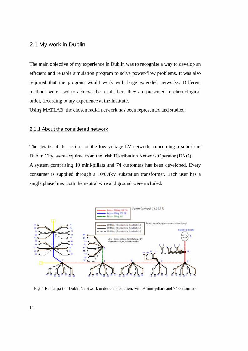
The details of the section of the low voltage LV network, concerning a suburb of
Dublin City, were acquired from the Irish Distribution Network Operator (DNO).
A system comprising 10 mini-pillars and 74 customers has been developed. Every
consumer is supplied through a 10/0.4kV substation transformer. Each user has a
single phase line. Both the neutral wire and ground were included.
Fig. 1 Radial part of Dublin’s network under consideration, with 9 mini-pillars and 74 consumers
14

The single-phase supplies at 230V and each consumer has a distinct earthing
arrangement that complies to TNC-S.
Service cabling from mini-pillars to consumers is modelled as overhead (25/16mm2
concentric neutral), whereas, for the cabling from the substation transformer to the
first mini-pillar and for each successive mini-pillar thereafter, 4-core, underground
cabling is employed (either 185/70mm2 cross-linked polyethylene XLPE, or 70mm2
paper-insulated NAKBA)[8].
The earth electrode is connected to the installation’s main earth terminal MET and
therefore to the DNO neutral. This arrangement provides the consumer with an earth
terminal, which is connected to the neutral conductor of the system, thereby
providing a low impedance path for the return of earth fault currents.
15

16

Chapter 3
The Backward-Forward method
When it is needed to find a solution for a a non-linear problem, like in the case of the
distribution network, iterative methods are the ones called to find an answer.
At first, at the Department the solution was sought adopting a backward-forward
method.
3.1 How it works
The Backward-Forward (B-F) is one of the techniques based on Ohm's and
Kirchhoff's laws and refers to aforementioned methods. There is also another
important family of what can be considered as classical processes that belongs to the
iterative methods. The Newton-Raphson’s is indeed one of the most developed and
usually chosen solution, since it requires a small number of iterations to reach the
result almost independently from the size of the system to solve. Unlike it, the B-F
needs many iterations to achieve the convergence. This might seem like a
disadvantage, however the time required by the CPU (Central Processing Unit) for
each iteration is shorter, so that the overall time spent to reach the final solution is
much lower than the one needed using a different family of classical methods. The
CPU time required at each iteration for the Newton-Raphson solution can be
considerably high if it is necessary to proceed to the matrix’s inversion.
So this technique uses a sweep load flow algorithm that suits for radial distribution
systems. The b-f method proceeds through four steps[2]:
17

1. the backward sweep uses Kirchhoff’s Voltage Law - KVL and the Kirchhoff’s
Current Law - KCL, to obtain the voltage at each upstream bus, the calculation of
the currents required by the loads and the lines shunt admittances, on the basis of
the calculated or fixed values of nodal voltages;
2. the evaluation of the current (or power) flows in the branches composing the
electrical system, starting from the terminal branches and going up to the source
node;
3. the nodes voltages calculation, starting from the source node and proceeding to the
terminal ones (forward sweep);
4. the verification of a convergence criterion; if it is satisfied the process stops,
otherwise it restarts from the first step.
There are three main variations of the b-f method that differ depending on the type of electric quantities calculated at each iteration in the backward step[5]:
a) the current summation method, in which the branch currents are evaluated;
b) the power summation method, in which the power flows in the branches are
evaluated;
c) the admittance summation method, in which, node by node, the driving point admittances are evaluated.
18
3.2 Representation of the line
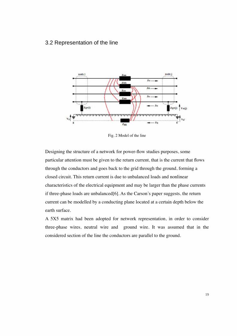
Fig. 2 Model of the line
Designing the structure of a network for power-flow studies purposes, some
particular attention must be given to the return current, that is the current that flows
through the conductors and goes back to the grid through the ground, forming a
closed circuit. This return current is due to unbalanced loads and nonlinear
characteristics of the electrical equipment and may be larger than the phase currents
if three-phase loads are unbalanced[6]. As the Carson’s paper suggests, the return
current can be modelled by a conducting plane located at a certain depth below the
earth surface.
A 5X5 matrix had been adopted for network representation, in order to consider
three-phase wires, neutral wire and ground wire. It was assumed that in the
considered section of the line the conductors are parallel to the ground.
19
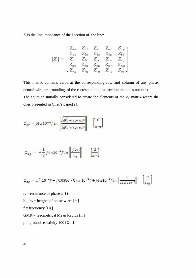
Zl is the line impedance of the l section of the line:
This matrix contains zeros at the corresponding row and column of any phase,
neutral wire, or grounding, of the corresponding line section that does not exist.
The equation initially considered to create the elements of the Zl matrix where the
ones presented in Ciric’s paper[2]:
ra = resistance of phase a [Ω]
ha , hb = heights of phase wires [m]
f = frequency [Hz]
GMR = Geometrical Mean Radius [m]
ρ = ground resistivity 100 [Ωm]
20
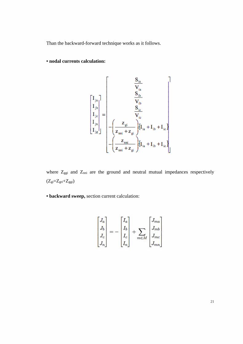
Than the backward-forward technique works as it follows.
• nodal currents calculation:
where Zggi and Znni are the ground and neutral mutual impedances respectively
(Zgi=Zgri+Zggi)
• backward sweep, section current calculation:
21
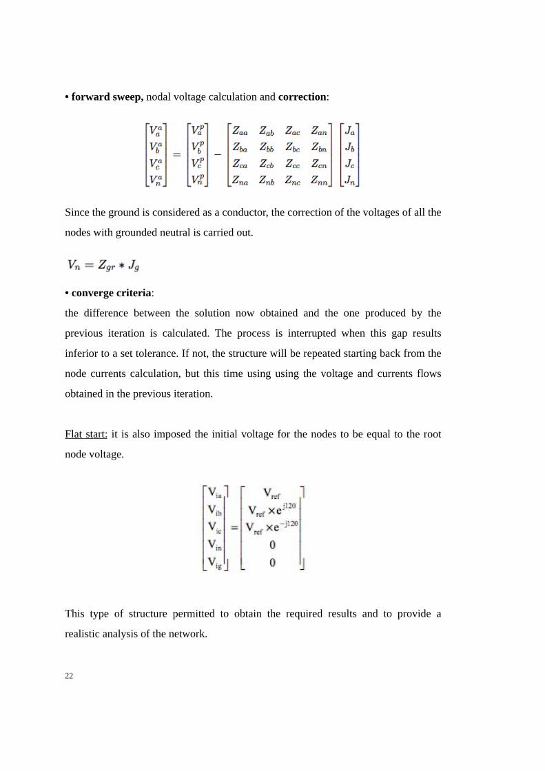
• forward sweep, nodal voltage calculation and correction:
Since the ground is considered as a conductor, the correction of the voltages of all the
nodes with grounded neutral is carried out.
• converge criteria:
the difference between the solution now obtained and the one produced by the
previous iteration is calculated. The process is interrupted when this gap results
inferior to a set tolerance. If not, the structure will be repeated starting back from the
node currents calculation, but this time using using the voltage and currents flows
obtained in the previous iteration.
Flat start: it is also imposed the initial voltage for the nodes to be equal to the root
node voltage.
This type of structure permitted to obtain the required results and to provide a
realistic analysis of the network.
22

It was observed anyway that to reach more accurate results the algorithm should be
modified to include Carson-Clem’s equation.
3.3 Carson-Clem’s equations
Ciric’s methodology had the inconvenience of not considering the finite conductivity
of the earth.
Carson’s equations permit to consider the influence of the earth resistance and of the
currents that flow through it.
Since a distribution feeder is inherently unbalanced, every analysis that would show
some precision should not make any assumptions regarding conductor sizes, the
spacing between conductors, and transposition. In order to face this problem of
accuracy, in his paper in 1926 Carson employed the image theory to develop
equations that calculate the self-impedance with earth return and mutual impedances
with common earth return for an arbitrary number of overhead conductors.
The image theory states that every conductor at a given distance above ground has an
image conductor the same distance below ground.
Carson assumed the earth is an infinite, uniform solid with a flat uniform upper
surface and a constant resistivity. Any end effects introduced at the neutral grounding
points are not large at power frequencies, and were therefore neglected[9].
These equations can also be applied to underground cables.
23
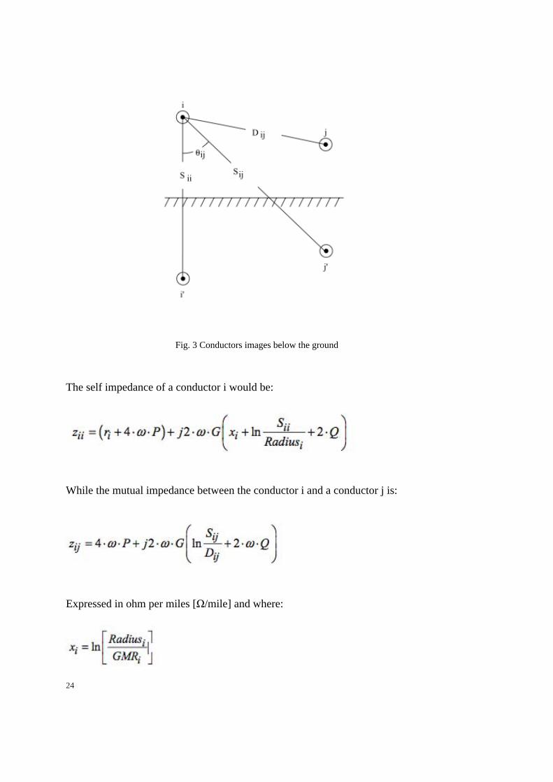
Fig. 3 Conductors images below the ground
The self impedance of a conductor i would be:
While the mutual impedance between the conductor i and a conductor j is:
Expressed in ohm per miles [Ω/mile] and where:
24

Radiusi = conductor radius in feet
GMRi = Geometric Mean Radius of conductor i in feet
zii= self impedance of conductor i in Ω/mile
zij= mutual impedance between conductors i and j in Ω/mile
ri = resistance of conductor i in Ω/mile
ω = 2πf = system angular frequency in radians per second
G = 0.1609344 × 10⁻³ Ω/mile
RDi = radius of conductor i in feet
f = system frequency in Hertz
ρ = resistivity of earth in Ω-meters
Dij = is the distance between the axis of the conductor with respect to the i-th and j-
th conductor;
Carson’s original equations were described in Ohms/mile, but the subsequent cabling
considerations that will be discussed here are described as Ohms/kilometre.
25

Anyway since the use of there equations was troublesome, some approximations
were made in deriving the modified Carson’s equations. These approximations were
firstly developed by Carson himself, involving the terms associated with Pij and Qij
by using only the first term of the variable Pij and the first two terms of Qij. So Pij
and Qij were defined as constants correction terms.
The technique was not met with a lot of enthusiasm because of the tedious
calculations that would have to be done on the slide rule and by hand. With the
advent of the digital computer, Carson’s equations have become widely used.
Anderson also derived equations to describe the self and mutual impedances of the
lines. He considers the Carson's line as a single return conductor with a self GMD of
1 foot (or 1 meter), located at a distance (unit length) above/below the over head or
under ground line, depending on the situation. This said distance is a function of the
earth resistivity. In his description of the cable impedances, Anderson employs the
concept of hypothetical return path of the earth current and is a function of both earth
resistivity and frequency.
Through these approximations new Carson’s equations where derived, here are
presented the Carson-Clem’s equations, which are the ones that were finally used in
the program.
Each conductor’s impedances are obtained according to Carson's formulas with the
following assumptions: the conductors are parallel to each other and the earth is
homogenous within a span.
The distance of the conductors from the centroid of the return currents in the ground
is defined as:
26
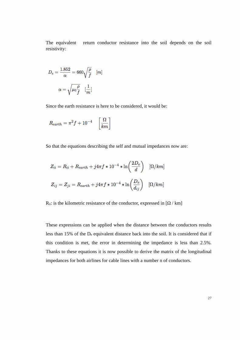
The equivalent return conductor resistance into the soil depends on the soil resistivity:
Since the earth resistance is here to be considered, it would be:
So that the equations describing the self and mutual impedances now are:
Rii: is the kilometric resistance of the conductor, expressed in [Ω / km]
These expressions can be applied when the distance between the conductors results
less than 15% of the De equivalent distance back into the soil. It is considered that if
this condition is met, the error in determining the impedance is less than 2.5%.
Thanks to these equations it is now possible to derive the matrix of the longitudinal
impedances for both airlines for cable lines with a number n of conductors.
27
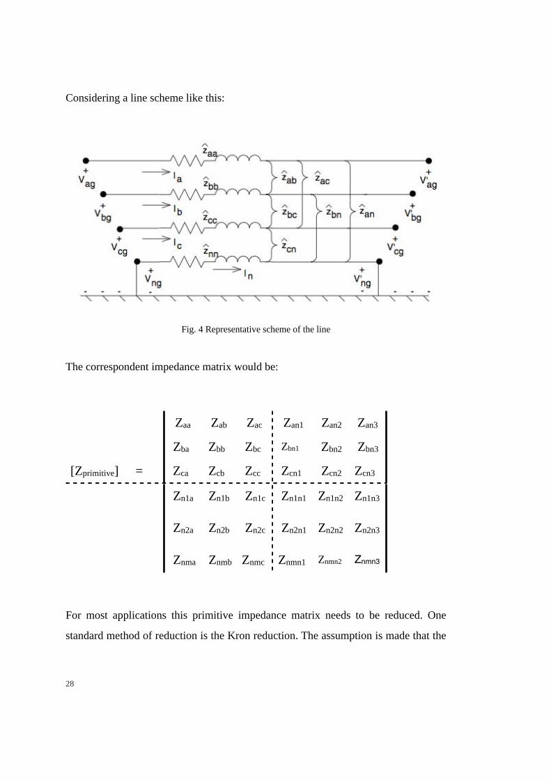
Considering a line scheme like this:
Fig. 4 Representative scheme of the line
The correspondent impedance matrix would be:
Zaa Zab Zac Zan1 Zan2 Zan3
Zba Zbb Zbc Zbn1 Zbn2 Zbn3
[Zprimitive] = Zca Zcb Zcc Zcn1 Zcn2 Zcn3
Zn1a Zn1b Zn1c Zn1n1 Zn1n2 Zn1n3
Zn2a Zn2b Zn2c Zn2n1 Zn2n2 Zn2n3
Znma Znmb Znmc Znmn1 Znmn2 Znmn3
For most applications this primitive impedance matrix needs to be reduced. One
standard method of reduction is the Kron reduction. The assumption is made that the
28

line has a multigrounded neutral. The Kron reduction method applies Kirchhoff’s
voltage law to the circuit.
By this simplification the matrix becomes:
that is:
Vabc =
V’abc +
Zij Zin *
Iabc
Vng V’ng Znj Znn In
Because the neutral is grounded, the voltages Vng and V’ng are equal to zero.
It means that the equation written above can now be re-written as:
[Vabc ] = [V’abc] + [Zij ]*[Iabc] + [Zin]*[In]
Which allows to solve the equation for:
29
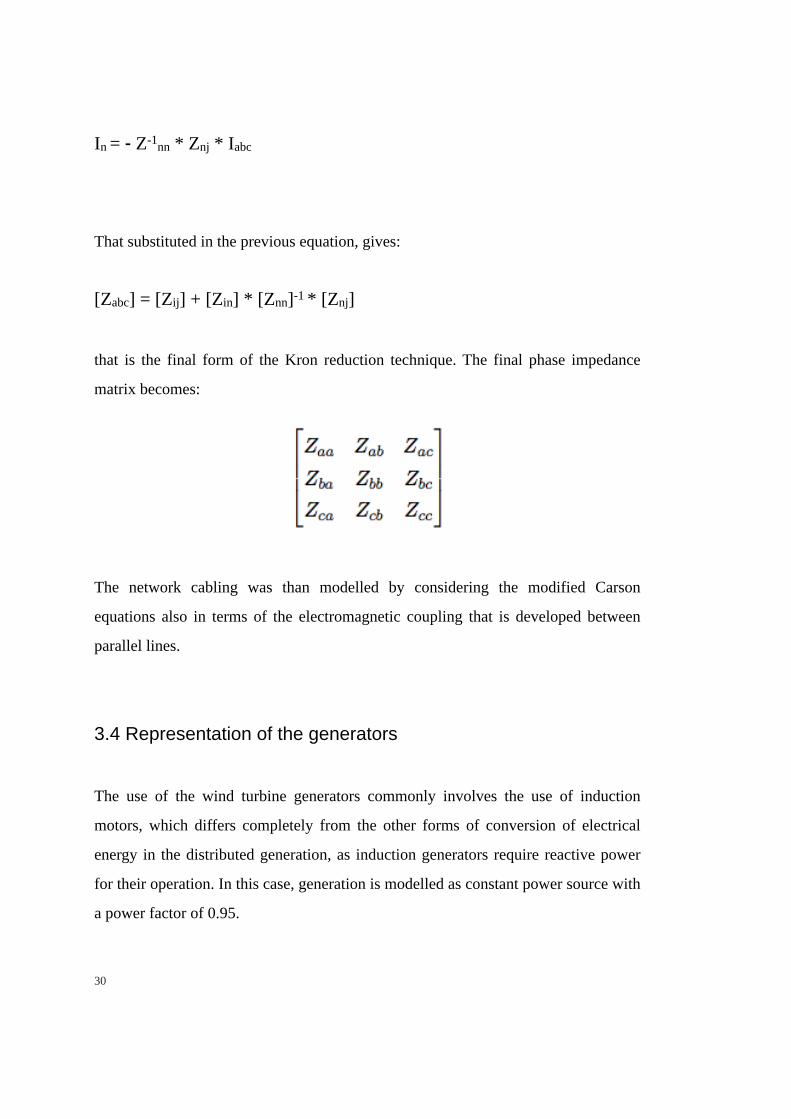
In = - Z-1nn * Znj * Iabc
That substituted in the previous equation, gives:
[Zabc] = [Zij] + [Zin] * [Znn]-1 * [Znj]
that is the final form of the Kron reduction technique. The final phase impedance
matrix becomes:
The network cabling was than modelled by considering the modified Carson
equations also in terms of the electromagnetic coupling that is developed between
parallel lines.
3.4 Representation of the generators
The use of the wind turbine generators commonly involves the use of induction
motors, which differs completely from the other forms of conversion of electrical
energy in the distributed generation, as induction generators require reactive power
for their operation. In this case, generation is modelled as constant power source with
a power factor of 0.95.
30

3.5 Representation of the loads
Depending on their type of the load its modelling changes. For the second step of the
backward-forward method this is a crucial point because it influences the nodal
currents calculation. In this work it has been considered to have a three-phase star or
phase to ground connection.
The diagram to refer to is this one:
Fig. 4 Load modelling scheme for three-phase star or phase to ground connection
3.6 Different implementations
Here are reported the scripts of the two different approaches to the construction of
the line impedances.
3.6.1 Ciric’s scheme
As it can be seen, in the first script proposed the earth resistance Re, and so the
distance of the conductors De, are neglected.
31
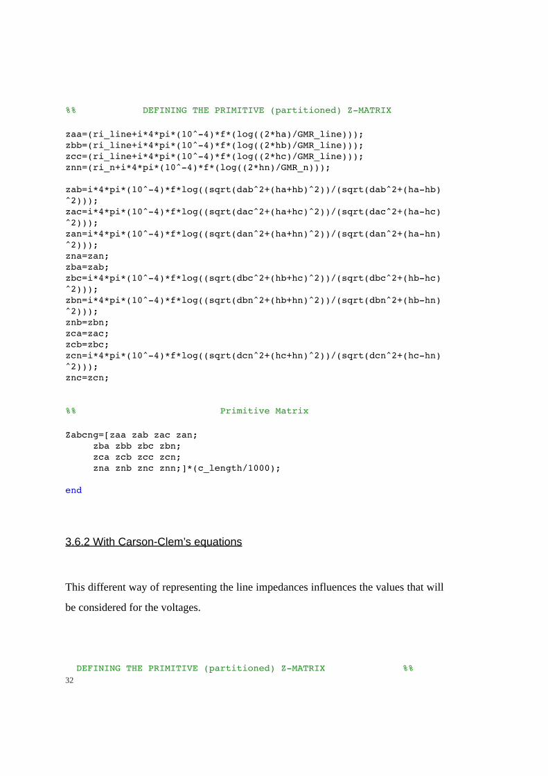
%% DEFINING THE PRIMITIVE (partitioned) Z-MATRIX
zaa=(ri_line+i*4*pi*(10^-4)*f*(log((2*ha)/GMR_line)));zbb=(ri_line+i*4*pi*(10^-4)*f*(log((2*hb)/GMR_line)));zcc=(ri_line+i*4*pi*(10^-4)*f*(log((2*hc)/GMR_line)));znn=(ri_n+i*4*pi*(10^-4)*f*(log((2*hn)/GMR_n))); zab=i*4*pi*(10^-4)*f*log((sqrt(dab^2+(ha+hb)^2))/(sqrt(dab^2+(ha-hb)^2)));zac=i*4*pi*(10^-4)*f*log((sqrt(dac^2+(ha+hc)^2))/(sqrt(dac^2+(ha-hc)^2)));zan=i*4*pi*(10^-4)*f*log((sqrt(dan^2+(ha+hn)^2))/(sqrt(dan^2+(ha-hn)^2)));zna=zan;zba=zab;zbc=i*4*pi*(10^-4)*f*log((sqrt(dbc^2+(hb+hc)^2))/(sqrt(dbc^2+(hb-hc)^2)));zbn=i*4*pi*(10^-4)*f*log((sqrt(dbn^2+(hb+hn)^2))/(sqrt(dbn^2+(hb-hn)^2)));znb=zbn;zca=zac;zcb=zbc;zcn=i*4*pi*(10^-4)*f*log((sqrt(dcn^2+(hc+hn)^2))/(sqrt(dcn^2+(hc-hn)^2)));znc=zcn;
%% Primitive Matrix
Zabcng=[zaa zab zac zan; zba zbb zbc zbn; zca zcb zcc zcn; zna znb znc znn;]*(c_length/1000); end
3.6.2 With Carson-Clem’s equations
This different way of representing the line impedances influences the values that will
be considered for the voltages.
DEFINING THE PRIMITIVE (partitioned) Z-MATRIX %%32

zaa=(ri_line+RE+i*4*pi*(10^-4)*f*(log(De/GMR_line)));zbb=(ri_line+RE+i*4*pi*(10^-4)*f*(log(De/GMR_line)));zcc=(ri_line+RE+i*4*pi*(10^-4)*f*(log(De/GMR_line)));znn=(ri_n+RE+i*4*pi*(10^-4)*f*(log(De/GMR_n))); zab=i*4*pi*(10^-4)*f*log((sqrt(dab^2+(ha+hb)^2))/(sqrt(dab^2+(ha-hb)^2)));zac=i*4*pi*(10^-4)*f*log((sqrt(dac^2+(ha+hc)^2))/(sqrt(dac^2+(ha-hc)^2)));zan=i*4*pi*(10^-4)*f*log((sqrt(dan^2+(ha+hn)^2))/(sqrt(dan^2+(ha-hn)^2)));zna=zan;zba=zab;zbc=RE+i*4*pi*(10^-4)*f*log(De/(sqrt(dbc^2+(hb-hc)^2)));zbn=RE+i*4*pi*(10^-4)*f*log(De/(sqrt(dbn^2+(hb-hn)^2)));znb=zbn;zca=zac;zcb=zbc;zcn=RE+i*4*pi*(10^-4)*f*log(De/(sqrt(dcn^2+(hc-hn)^2)));znc=zcn; %% Primitive Matrix
Zabcng=[zaa zab zac zan; zba zbb zbc zbn; zca zcb zcc zcn; zna znb znc znn;]*(c_length/1000); end
Since the criteria at the basis of the convergence is the difference between two
voltages, when these values changes, the range for the reaching of the solution
becomes too big to permit the program to stop after a reasonable number of
iterations.
It does not mean that the modified program is wrong. On the contrary, this attempt of
changing the characteristic of the line has highlighted the limits of the b-f technique,
which where there from the beginning.
33

3.7 Which is the actual issue
Cable models are very influential in deriving any power flow solution aiming to
derive accurate voltage profile results.
Using Kron’s reduction in fact, the information regarding the neutral voltages gets
lost, since this value is forced to zero along the line. This type of imposition results
much stronger as the network starts to present increasing levels of unbalancing.
It is thanks to that that the iteration could reach a solution, while it would be
impossible when including the earth connection. By this approximation the network
is changed in structure, considering the earth connection only at the substation (like
in Italy), but not at the bus nodes (like in Ireland).
Including the Carson-Clem’s equations the converging criteria of the developed
network does not permit to reach a solution.
It was initially supposed it was because of the criteria for applying the formulas had
not been respected. So it was verified that also in this case the distance between the
conductors resulting less than 15% of the equivalent distance of the return conductor
into the soil De. Anyway the distance was proved appropriate.
The correction that Carson introduced to taken into account the finite value of the
resistivity of the soil, for the calculation of the line impedances, can indeed result as
the predominant term of the equation. In facts, referring to the scripts here reported,
it results that De can be much bigger that ha, with predictable results changes.
When Ciric’s equation are considered, this fact is neglected as for the Re and De.
The impossibility for this algorithm to converge is due to the fact that, since the
convergence depends on a range of voltages, using these new formulas a greater
voltage variation is now introduced. The backward-forward method no longer suits.
Anyway the most important aspect to be considered is the chosen configuration for
the line, which includes multi-grounded neutral. This is a key point in the reach of 34

the solution. What indeed does not permit to prefer the backward-forward model in
this case is that with Ciric’s approach the voltage in the neutral tends to show very
little variations, remaining almost constant. This type of condition is in this program
forced, ignoring the earth loads and pillars connections that are characteristic of the
Irish network that present the multi-grounded neutral configuration.
It is also the reason why, when the same script was applied to the Italian network,
where the neutral is grounded only in the substations, the program including the
Carson-Clem variation worked.
35

36
Chapter 4
Analysis of the Network Structure
The two systems presented above have been manipulated to obtain smaller and easier
to manage networks, reducing the pillars from 9 to 2, changing the numbers of loads
as well. This operation was made in order to permit a deeper investigation of the
backward-forward method and so to achieve to find, if not a solution, a reason for the
not proper working of Ciric’s approach when including the Carson-Clem’s equations.
Here in this section are reposted the result obtained ingnoring the earth connection.
4.1 B-F algorithm structure
Here are reported the most important functions and variables in the program, for a
better comprehension of its development. As it can be seen in Appendix A, the
program proposes two different ways to consider the lines, including or excluding the
earth connection. It is in fact this type of connection that leads to more uncertainties
and has in this way been highlighted.
In this analysis the parameters regarding the earth will be included.
Starting from the main program, here are presented the scripts, trying to give them an
order meant to facilitate an immediate understanding.
37

4.1.1 Model_Entire_Network
• the the system parameters are defined, such as power and voltage
V_line = 415;Sys_MVA_base = 1e+6;z_base = V_line^2/(Sys_MVA_base);
• fundamental sub-programs are called. In here there are the:
- System_Z, to define the network impedances
- Inital_Voltage, to assign the flat start to all system’s buses
- Customer_Load_With_EarthElectrode, deriving the comsumers loads from the .txt
file containing the active and reactive parameters for each bus
- Branch_Current, evaluating branch and pillars’ currents
•the loop flow is initialised for the calculation of voltages and currents
for ii=1:369 V_Diff=V_3; ii Voltage_Update if max(abs(V_Diff-V_3))<0.00001 break end Customer_Load_With_EarthElectrode Branch_Current V_3 end
• the RESULTS are called out
4.1.2 Sys_Load
Active and reactive powers P and Q are uploaded for each bus from a Load.txt file,
together with the related voltages from the Customer_Load_With_EarthElectrode
file.
38

This program calculates loads S power and provides loads current for each phase at
each bus.
function [Sabc, Iabcng]= Sys_Load(bus, V)
Sabc=[Load(row_ID,2)+j*Load(row_ID,3) Load(row_ID,4)+j*Load(row_ID,5) Load(row_ID,6)+j*Load(row_ID,7)];
Ia=conj(Sabc(1))./(conj(V(1)-V(4)));Ib=conj(Sabc(2))./(conj(V(2)-V(4)));Ic=conj(Sabc(3))./(conj(V(3)-V(4)));
In=-(Ia+Ib+Ic)+(V(4))/Rcons;
4.1.3 Branch_Current
Gives the sum of loads currents, neutral currents included, to obtain pillar currents,
updating them at each node.
%Pillar B Pillar=1; I_46=IL_46;I_63=IL_63;I_75=IL_75;I_59=IL_59;I_26=IL_26;I_120=IL_120; I_2=I_46+I_63+I_75+I_59+I_26+I_120+I_3; I=I_2; Rg_pillar=R_Pillar_Electrode; [I_Pillar]= Pillar_Current(Pillar,I,V_2,Rg_pillar); I_2=I_Pillar; % SUBSTATION A I_1=I_2;
4.1.4 Pillar_Current
The sum of loads currents calculated in the Branch_Current does not gives the pillar
current. It is in fact necessary to consider the pillar earth connection through the
inclusion of the current due to the voltage trop in Rg_Pillar.
function [I_Pillar]= Pillar_Current(Pillar, I,V,Rg_pillar) Pillar;
39
In=I(4)+(V(4))/Rg_pillar; I_Pillar=[I(1);I(2); I(3); In;];
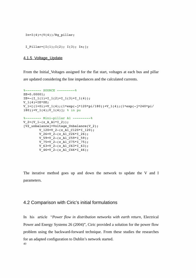
4.1.5 Voltage_Update
From the Initial_Voltages assigned for the flat start, voltages at each bus and pillar
are updated considering the line impedances and the calculated currents.
%-------- SOURCE ---------%ZE=0.00001;IE=-(I_1(1)+I_1(2)+I_1(3)+I_1(4));V_1(4)=IE*ZE;V_1=[(1+0i)+V_1(4);(1*exp(-j*120*pi/180))+V_1(4);(1*exp(-j*240*pi/180))+V_1(4);V_1(4)]; % in pu %-------- Mini-pillar A1 ---------%V_2=(V_1-(z_A_A1*I_2));[V2_unbalance]=Voltage_Unbalance(V_2); V_120=V_2-(z_A1_C120*I_120); V_26=V_2-(z_A1_C26*I_26); V_59=V_2-(z_A1_C59*I_59); V_75=V_2-(z_A1_C75*I_75); V_63=V_2-(z_A1_C63*I_63); V_46=V_2-(z_A1_C46*I_46);
The iterative method goes up and down the network to update the V and I
parameters.
4.2 Comparison with Ciric’s initial formulations
In his article “Power flow in distribution networks with earth return, Electrical
Power and Energy Systems 26 (2004)”, Ciric provided a solution for the power flow
problem using the backward-forward technique. From these studies the researches
for an adapted configuration to Dublin’s network started.40
To evaluate the DIT proposed program, it is then important to compare it from where
it was firstly created.
The crucial steps for the script development are here reported in association with
Ciric’s ideas.
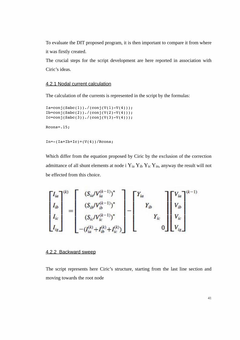
4.2.1 Nodal current calculation
The calculation of the currents is represented in the script by the formulas:
Ia=conj(Sabc(1))./(conj(V(1)-V(4)));Ib=conj(Sabc(2))./(conj(V(2)-V(4)));Ic=conj(Sabc(3))./(conj(V(3)-V(4))); Rcons=.15; In=-(Ia+Ib+Ic)+(V(4))/Rcons;
Which differ from the equation proposed by Ciric by the exclusion of the correction
admittance of all shunt elements at node i Yia Yib Yic Yin, anyway the result will not
be effected from this choice.
4.2.2 Backward sweep
The script represents here Ciric’s structure, starting from the last line section and
moving towards the root node
41
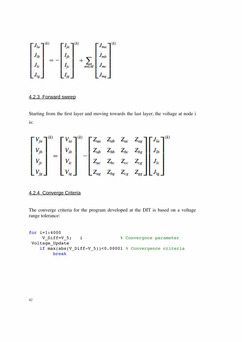
4.2.3 Forward sweep
Starting from the first layer and moving towards the last layer, the voltage at node i
is:
4.2.4 Converge Criteria
The converge criteria for the program developed at the DIT is based on a voltage range tolerance:
for i=1:4000 V_Diff=V_5; i % Convergnce parameter Voltage_Update if max(abs(V_Diff-V_5))<0.00001 % Convergence criteria break
42
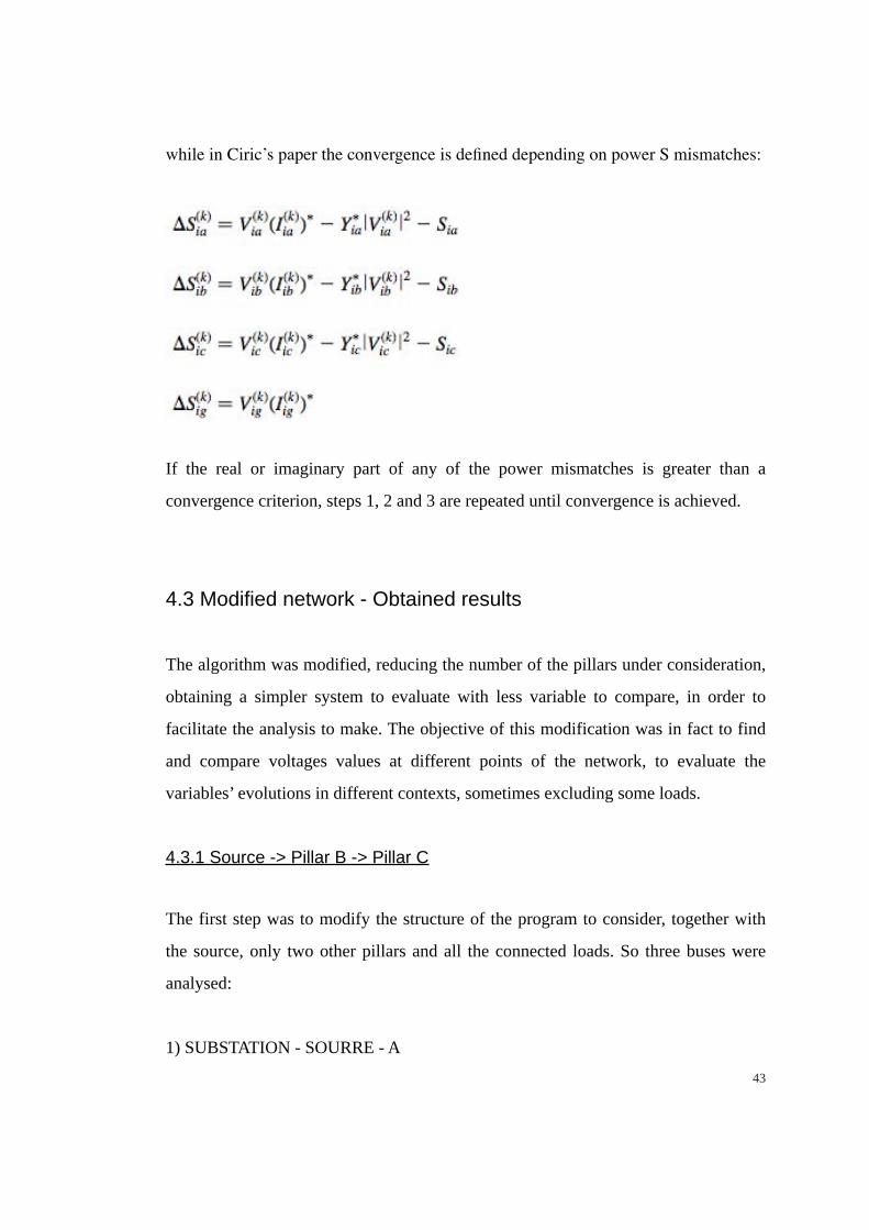
while in Ciric’s paper the convergence is defined depending on power S mismatches:
If the real or imaginary part of any of the power mismatches is greater than a
convergence criterion, steps 1, 2 and 3 are repeated until convergence is achieved.
4.3 Modified network - Obtained results
The algorithm was modified, reducing the number of the pillars under consideration,
obtaining a simpler system to evaluate with less variable to compare, in order to
facilitate the analysis to make. The objective of this modification was in fact to find
and compare voltages values at different points of the network, to evaluate the
variables’ evolutions in different contexts, sometimes excluding some loads.
4.3.1 Source -> Pillar B -> Pillar C
The first step was to modify the structure of the program to consider, together with
the source, only two other pillars and all the connected loads. So three buses were
analysed:
1) SUBSTATION - SOURRE - A
43
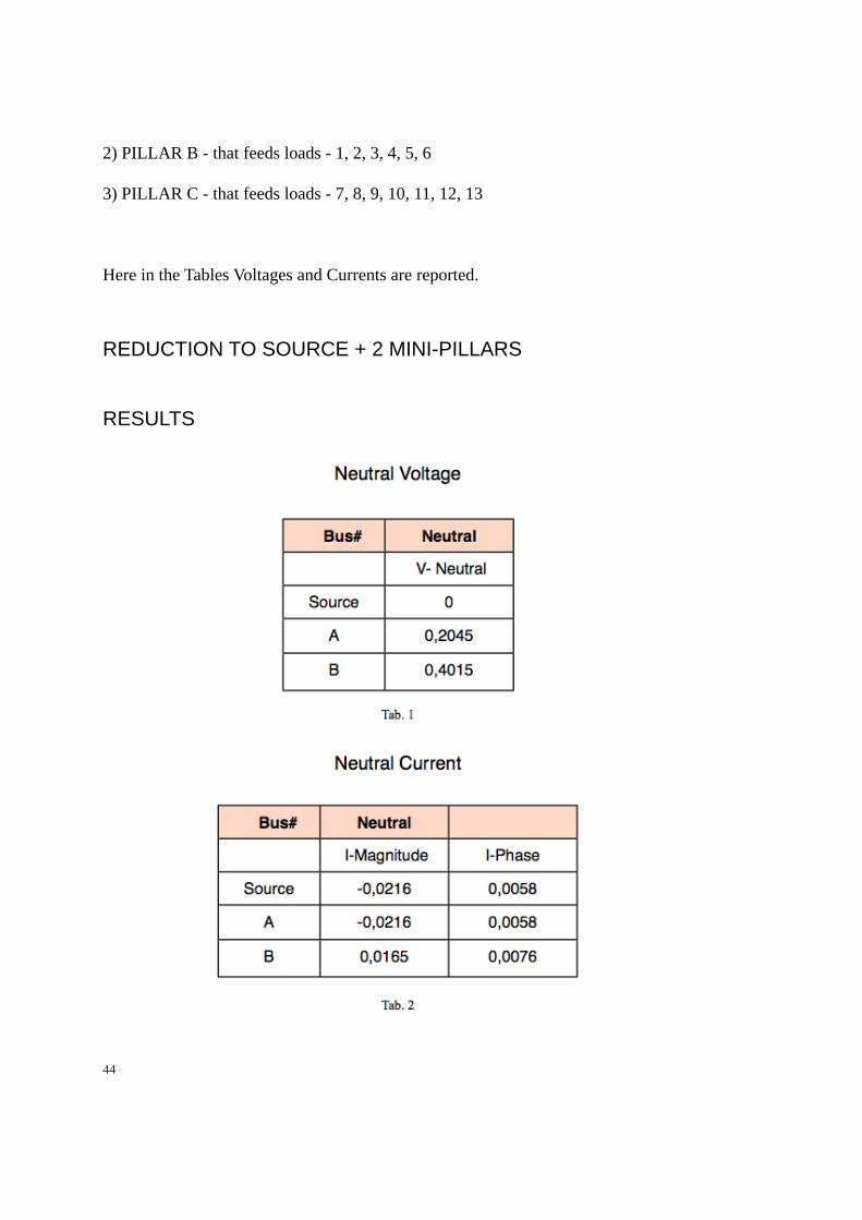
2) PILLAR B - that feeds loads - 1, 2, 3, 4, 5, 6
3) PILLAR C - that feeds loads - 7, 8, 9, 10, 11, 12, 13
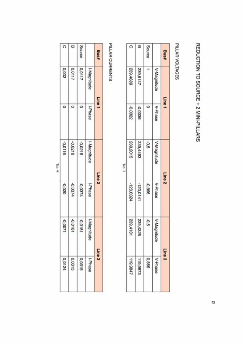
Here in the Tables Voltages and Currents are reported.
REDUCTION TO SOURCE + 2 MINI-PILLARS
RESULTS
44
45
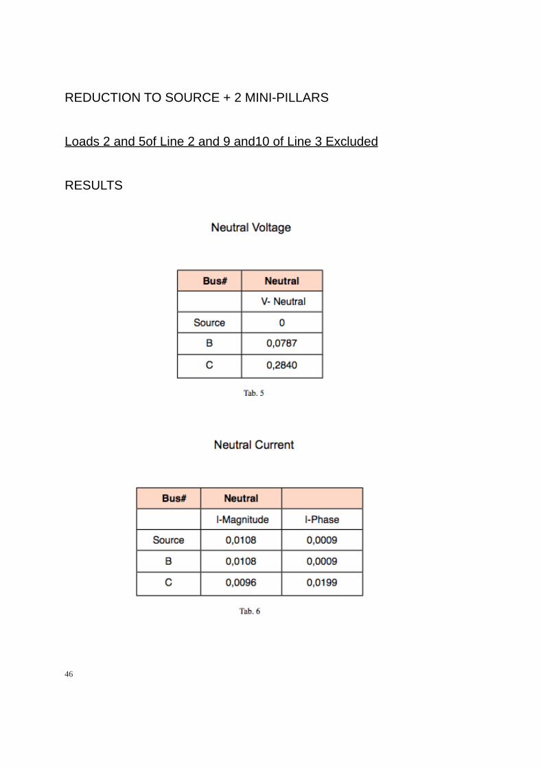
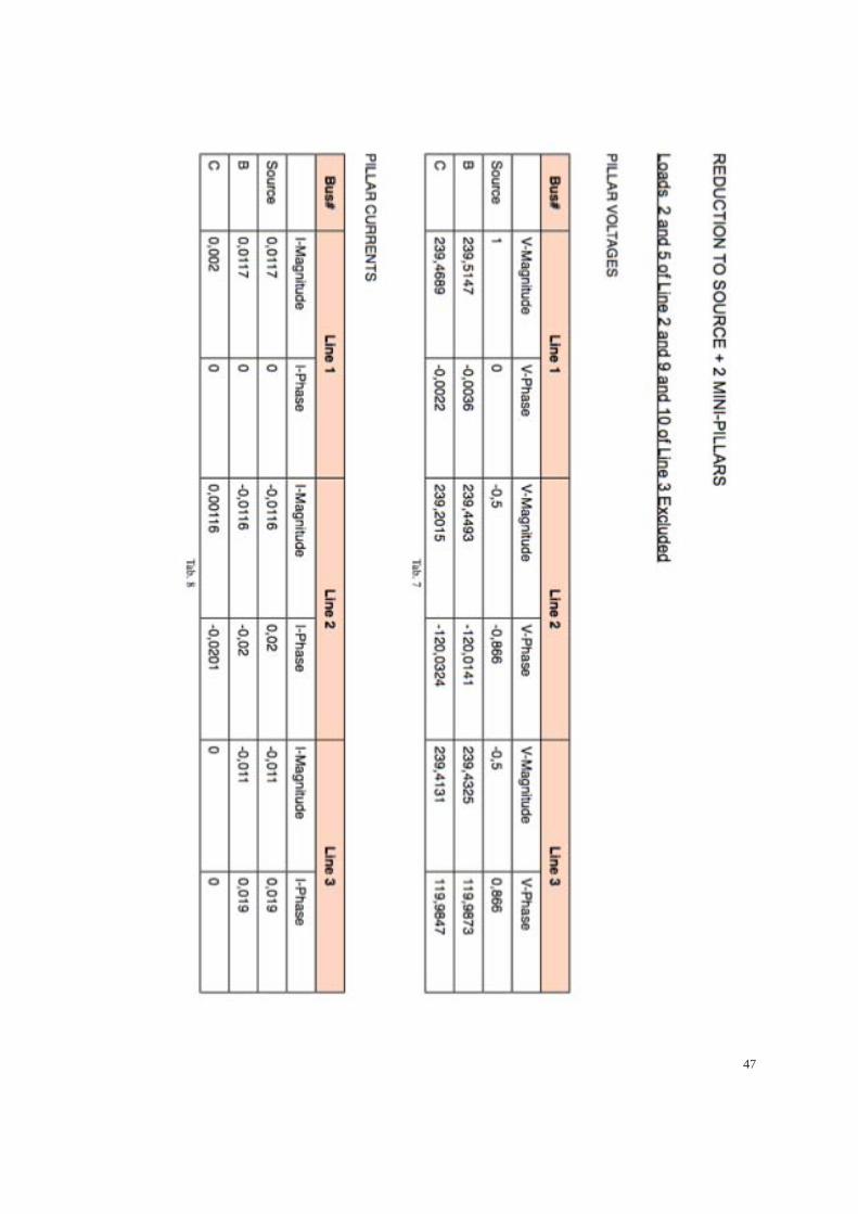
REDUCTION TO SOURCE + 2 MINI-PILLARS
Loads 2 and 5of Line 2 and 9 and10 of Line 3 Excluded
RESULTS
46
47

48
Chapter 5
The Complex Admittance Method
5.1 Why another method investigation
The backward-forward method has some positive peculiarities and thanks to its
speed and solidity this method is the subject of considerable study and
improvements. It has been demonstrated anyway that it is not always appropriate to
any type of network, especially when applying Carson - Clem’s formulas to a
network that is structured so that each consumer has an earth electrode connection to
earth.
On the other hand there were still some researches I had to do on regards of the
CAM method, to clarify it’s proprieties and strengths.
Once the experience at the DIT was over, my researches regarding the CAM method
needed to be deepened in order to provide an adequate comparison between the two
models. In this case in particular I had to look for other theoretical references, as my
work was initially mainly based on the article [10].
5.2 New network representation
Most of the methods have been developed to study transmission systems. Over the
years variations of the Newton method (such as the fast decoupled method) have
become the most widely used. However, even though the Newton-Raphson
49

technique is still a valid choice in the resolutions of the transmission networks, it can
not be directly applied to the distribution networks because of some features of the
latter distribution networks that need a different approach for its load flow analysis.
These characteristics are[4]:
• high ratio R / X of the feeder;
• asymmetry of the network;
• imbalance of loads;
• high number of nodes.
Thanks to the approach here presented, it is anyway possible to achieve a power flow
solution also in those systems with high R / X ratio in some lines and in situations
close to voltage collapse.
The procedure is sufficiently robust to facilitate a multi-conductor asymmetrical
network analysis. The methodology was originally developed for computing
electromagnetic coupling of complex conductor geometries, incorporating network
structure, load, generation and earthing elements.
It is thus based on the formal possibility to represent both loads and generators,
except for the slack-bus, by shunt elements, which will be included in a nodal
admittance matrix.
50
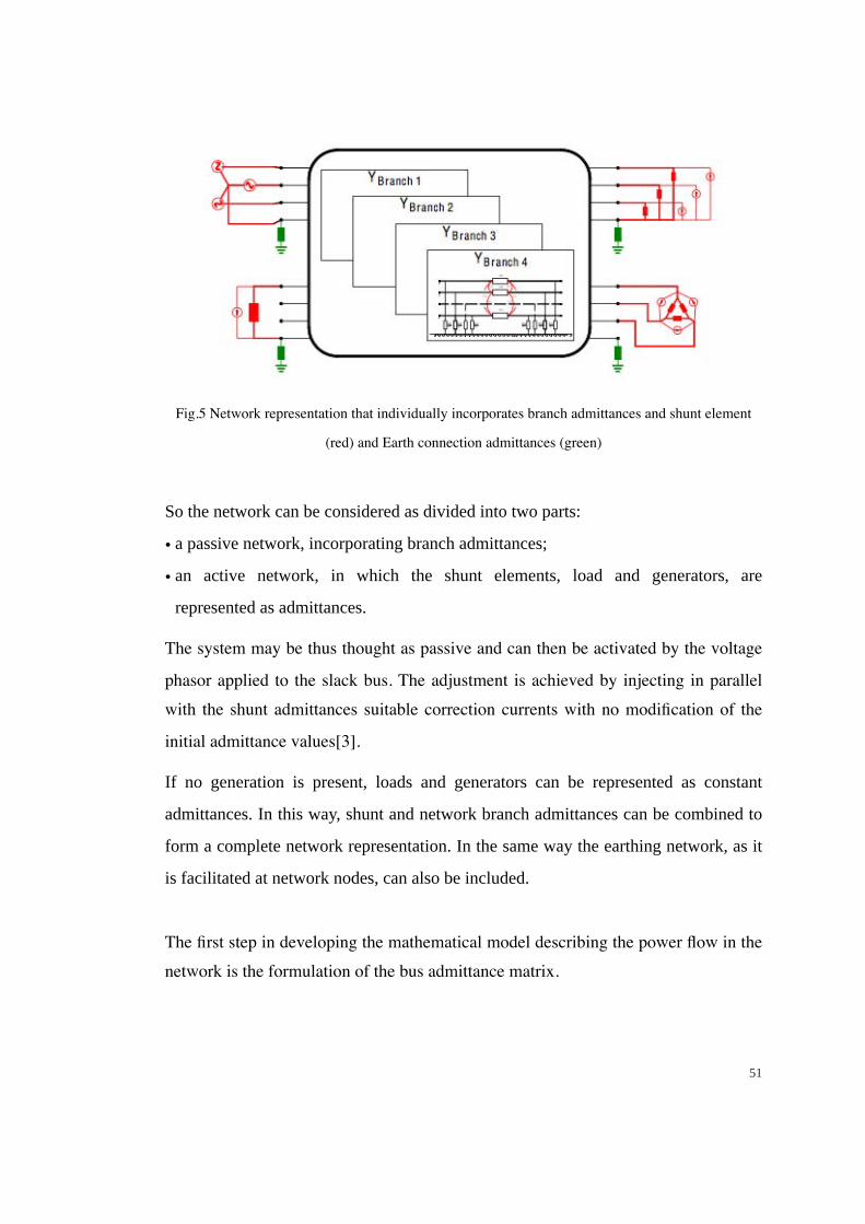
Fig.5 Network representation that individually incorporates branch admittances and shunt element
(red) and Earth connection admittances (green)
So the network can be considered as divided into two parts:
• a passive network, incorporating branch admittances;
• an active network, in which the shunt elements, load and generators, are
represented as admittances.
The system may be thus thought as passive and can then be activated by the voltage
phasor applied to the slack bus. The adjustment is achieved by injecting in parallel with the shunt admittances suitable correction currents with no modification of the
initial admittance values[3].
If no generation is present, loads and generators can be represented as constant
admittances. In this way, shunt and network branch admittances can be combined to
form a complete network representation. In the same way the earthing network, as it
is facilitated at network nodes, can also be included.
The first step in developing the mathematical model describing the power flow in the network is the formulation of the bus admittance matrix.
51
5.3 The admittance matrix
Includes branch and shunt elements and expresses the relationship between the
currents and the voltages.
It is a symmetric matrix along the leading diagonal, which result in an upper
diagonal nodal admittance matrix. The diagonal elements are the self-admittances at
the nodes and the other components are the mutual admittances.
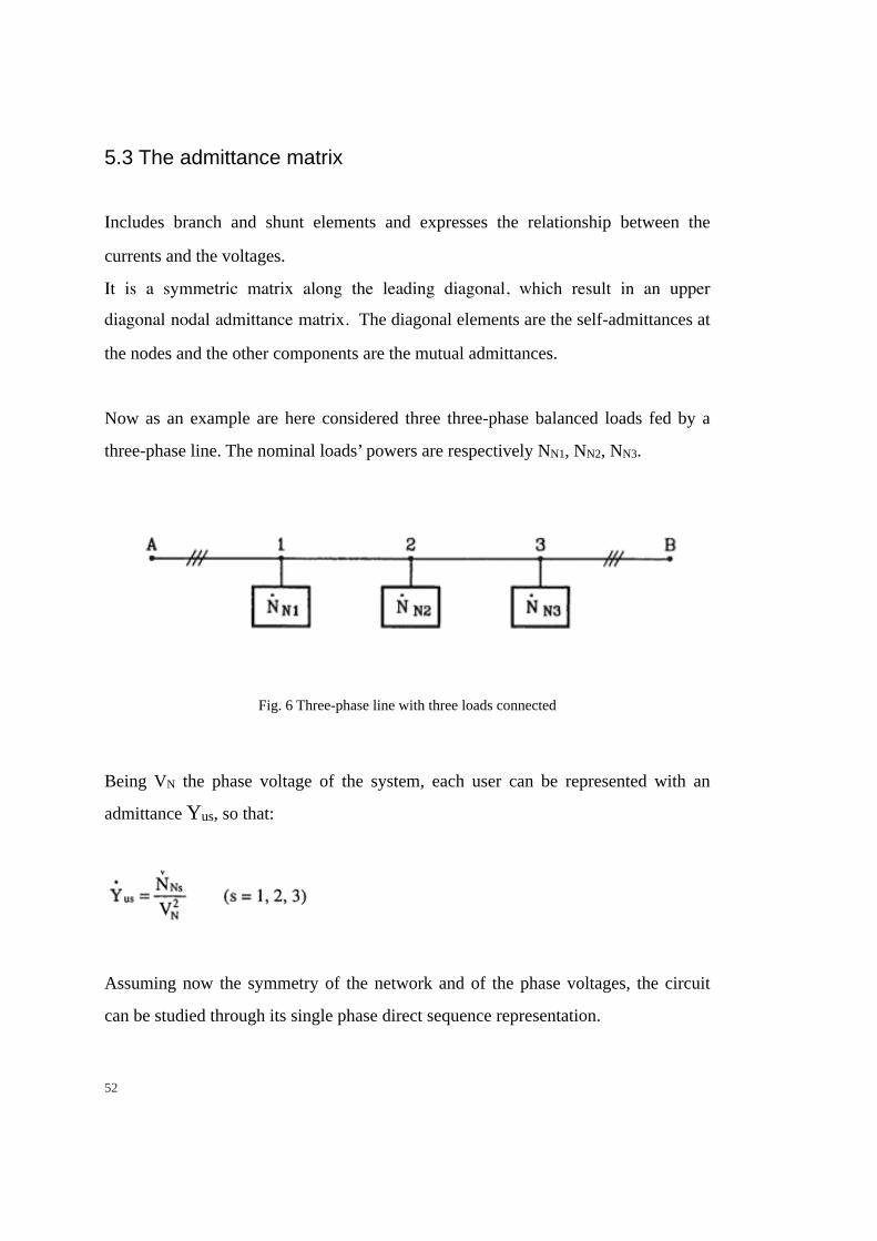
Now as an example are here considered three three-phase balanced loads fed by a
three-phase line. The nominal loads’ powers are respectively NN1, NN2, NN3.
Fig. 6 Three-phase line with three loads connected
Being VN the phase voltage of the system, each user can be represented with an
admittance Yus, so that:
Assuming now the symmetry of the network and of the phase voltages, the circuit
can be studied through its single phase direct sequence representation.
52
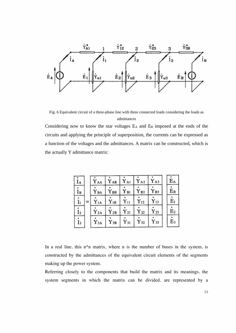
Fig. 6 Equivalent circuit of a three-phase line with three connected loads considering the loads as
admittances
Considering now to know the star voltages EA and EB imposed at the ends of the
circuits and applying the principle of superposition, the currents can be expressed as
a function of the voltages and the admittances. A matrix can be constructed, which is
the actually Y admittance matrix:
In a real line, this n*n matrix, where n is the number of buses in the system, is
constructed by the admittances of the equivalent circuit elements of the segments
making up the power system.
Referring closely to the components that build the matrix and its meanings, the
system segments in which the matrix can be divided, are represented by a
53
combination of shunt elements, connected between a bus and the reference node, and
series elements, connected between two system buses. Each of these segments can be
represented by a π-circuit.
Cascade connections of multiphase π-circuits can be easily used to model each span
and, consequently, the full length of the line without any limits in the number of phase
conductors.
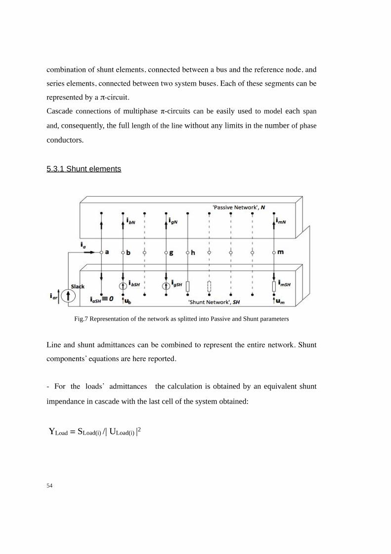
5.3.1 Shunt elements
Fig.7 Representation of the network as splitted into Passive and Shunt parameters
Line and shunt admittances can be combined to represent the entire network. Shunt
components’ equations are here reported.
- For the loads’ admittances the calculation is obtained by an equivalent shunt
impendance in cascade with the last cell of the system obtained:
YLoad = SLoad(i) /| ULoad(i) |2
54
- while the generators admittances are:
YLoad = SGen(i) /| UGen(i) |2
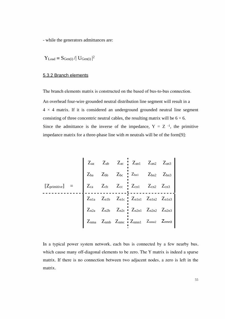
5.3.2 Branch elements
The branch elements matrix is constructed on the based of bus-to-bus connection.
An overhead four-wire grounded neutral distribution line segment will result in a
4 × 4 matrix. If it is considered an underground grounded neutral line segment
consisting of three concentric neutral cables, the resulting matrix will be 6 × 6.
Since the admittance is the inverse of the impedance, Y = Z -1, the primitive
impedance matrix for a three-phase line with m neutrals will be of the form[9]:
Zaa Zab Zac Zan1 Zan2 Zan3
Zba Zbb Zbc Zbn1 Zbn2 Zbn3
[Zprimitive] = Zca Zcb Zcc Zcn1 Zcn2 Zcn3
Zn1a Zn1b Zn1c Zn1n1 Zn1n2 Zn1n3
Zn2a Zn2b Zn2c Zn2n1 Zn2n2 Zn2n3
Znma Znmb Znmc Znmn1 Znmn2 Znmn3
In a typical power system network, each bus is connected by a few nearby bus,
which cause many off-diagonal elements to be zero. The Y matrix is indeed a sparse
matrix. If there is no connection between two adjacent nodes, a zero is left in the
matrix.
55

That in the partitioned form might also result like:
[Zprimitive] = Zij Zin
Znj Znn
5.4 System Complex Admittance Matrix
The entire matrix is built by placing branch element sub-matrices into the system
through a topology matrix. In the same way, earth connections may be defined by
adding self-admittances to the neutral conductor at the relative bus.
It is generally the branch matrix to be constructed firstly and then this primary block
is expanded adding the ones regarding the connection admittances and the loads or
generators admittances.
Loads are usually expressed as a series admittance, following the last segment
obtained from the branch admittances’ representation. If any constant-power load is
present, an iterative method would be necessary to evaluate the equivalent current
injection depending on the nodal voltage.
Generators are represented by a complex vector composed of two shares: one made
of voltages’ magnitude and phase, the other made of unknown elements.
Considering now the network under analysis, there will be a matrix representing the
4-wire branches that link each pillar to each others to which are added the parts of
the consumers’ connections’ admittances and the loads and generators’ shunt
admittances.
56
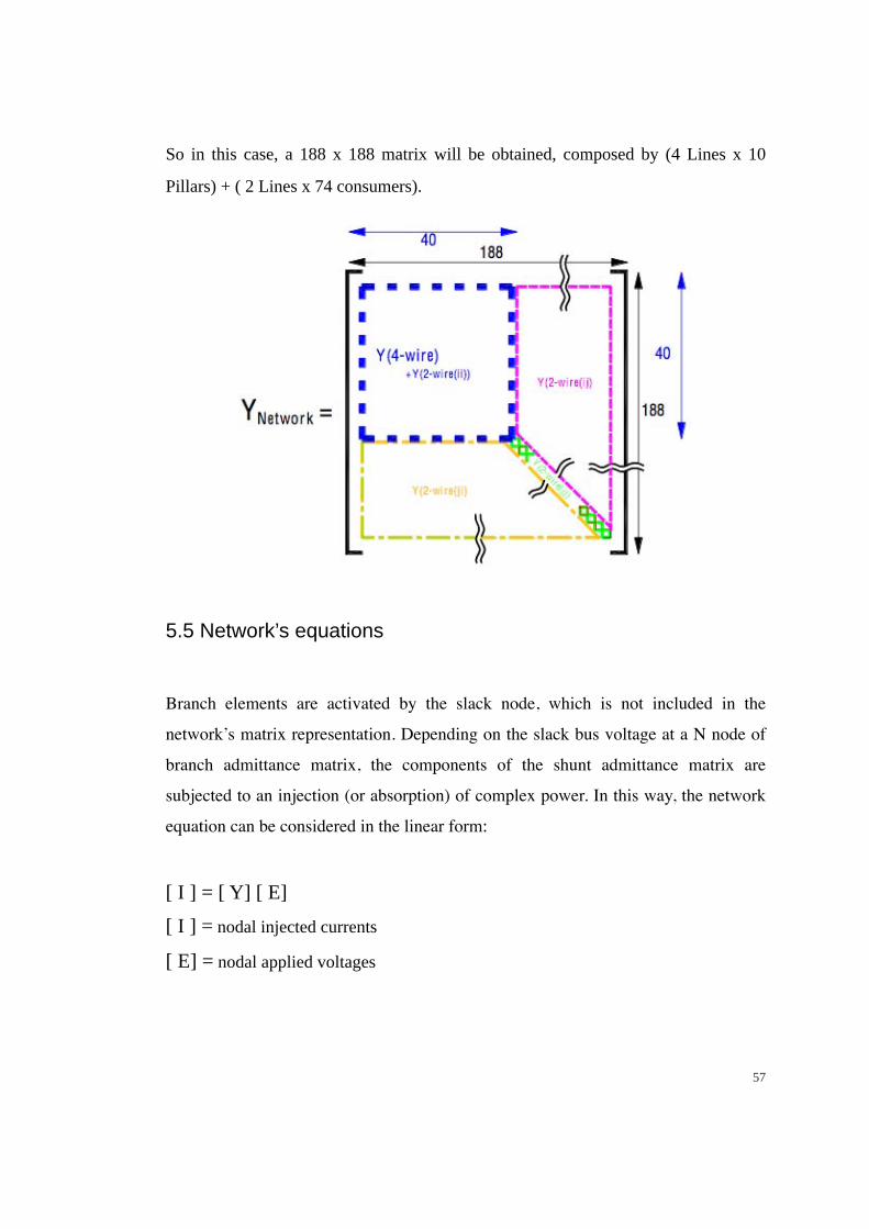
So in this case, a 188 x 188 matrix will be obtained, composed by (4 Lines x 10
Pillars) + ( 2 Lines x 74 consumers).
5.5 Network’s equations
Branch elements are activated by the slack node, which is not included in the
network’s matrix representation. Depending on the slack bus voltage at a N node of
branch admittance matrix, the components of the shunt admittance matrix are
subjected to an injection (or absorption) of complex power. In this way, the network
equation can be considered in the linear form:
[ I ] = [ Y] [ E]
[ I ] = nodal injected currents
[ E] = nodal applied voltages
57

Where:
Y = YN + YSH
So now the matrix describing the network can be re-written as:
ia YGG
YGL
ua
0 =
YGG
YGL
* ...
... YLG YLL
...
0
YLG YLL
um
That also means:
iG = YGG * uG + YGL * uL
0 = YGL * uG + YLL * uL
That leads to:
uL = - YLL-1 * YLG* uG
and consequently to:
iG = YGG + YGL * (- YLL-1 * YLG)]* uG
58

The above matrix can be again divided according to the last current equation derived.
In this way the system can be seen as formed as:
ia A
B
uar
= C D
*
ix
C D
ux
Since [ I] stands for all the currents that are injected and that ix represents only the
loads’ currents, ix = 0:
0 = C * uar + D * ux
ux = - D-1 * C * uar
The system supply current can be described with the equation:
ia = A * uar + B *( D-1 * C * uar )
This procedure can be applied at any section of the net, to evaluate voltage and
current at each segment.
The power flow problem can be iteratively solved through the application of a
certain voltage at the slack node, in association with a network admittance matrix
representation. The solution can be obtained by setting a flat start to the shunt
elements and each network bus. Successive values of system voltage are acquired
from every iteration by varying the shunt admittances of both generator and load
buses in order to satisfy the required voltage and power values.
59

5.6 CAM Algorithm structure
5.6.1 Main
The algorithm is structured in terms of four components:
1. a program to facilitate the derivations of the 4-wire (backbone) system y-matrix;
2. a program that facilitates the inclusion of the 2-wire (consumer connections);
3. the pillar earth electrode resistance is compiled as a matrix which is added to the
system y-matrix; the consumer earth electrode representation is included when
the consumer loads are referenced;
4. the load flow solution is derived in two stages: the consumer load is called, the
load flow is implemented.
5.6.2 4-wire and 2-wire admittance matrixes
There are two programs that contain functions to read, CVS files ( 4wirebuses.csv
and 2wirebuses.csv ), that recall definitions to describe the lines as considered from
bus (fb), to-bus (tb), the line configuration ( that defines the type of 4-wire cable) and
the line length.
The 4-wire Y-matrix is derived in terms of the fb/tb parameters in terms of the off
diagonal and then diagonals.
After gaining the cognisance of the consumer connections to the 4-wire backbone,
the Y-matrix system can be extended to represent the single-phase consumer line
connections individually.
60

5.6.3 Earth Elect
This programme defines, in terms of the network description parameters, the
connections of the pillar earth electrodes, which means, each pillar accommodates an
earth electrode.
The programme also defines the consumer earth electrode resistance.
5.6.4 2-Wire Y system
This program has four principal aspects:
1) one subprogram defines the flat voltage configuration;
2) the voltage difference tolerance, iteration count and the maximum number of
iterations allowed is defined;
3) a function is used to redefine the consumer load into an admittance proportional
to the derived consumer voltage;
4) this function load into a 2x2 construct which can be included in the system Y-
matrix.
5.6.5 Results
This file derives a data file which presents the voltage calculated across the network,
in terms of the 4-wire backbone and single-phase consumer connections.
The idea promoted at the DIT was to gain a quicker and more generalizable
procedure.
61

Thanks to this method a solution can be found, managing to include the Carson-
Clem’s equations.
62

Chapter 6
Conclusions
6.1 The Actual Comparison
The two different programs described propose not so different results when earth
electrodes are not included in the b-f iteration. It is anyway possible to guess which
is the more reliable one, since the CAM methodology has shown from the beginning
clearer methodology and development. The same principle has also been re-used by
our Department at the University of Padova to elaborate another program with the
same purposes.
In order to better analyse the peculiarities of these approaches, a comparison
regarding the results obtained from each of them are highlighted. It must be repeted
though that the results here reported from the b-f refer to the absence fo the earth
connection. In fact including this connection the results are unavailable.
The results obtained by the b-f method with Ciric’s approach show reliablility
because of the specific type of network under consideration. Kron simplifications,
that had being used, can be thought as representative of the Irish network structure
that includes the use of the multigrounded neutral. This is the reason why once
including Carson - Clem’s formulas the program will not reach a solution, though in
this way it would provide a more valid approach since it could be applied to any type
of network.
Since, as far as I am concerned, the program created in Ireland has a coherent and
reliable structure, the problem of its in-adaptability must be looked up somewhere in
its principles, as so, in the application of Carson’s formulas. So I would say that the
similarities of the results of the different approaches depend on the use of Kron’s
63

reduction. This approach applied to that type of network representation affects the
vision of the network itself, making it almost irrelevant the values of the grounding
impedances of the neutral with regard to the loads and the pillars, thus giving much
weight to the grounding in the substation A.
Anyway since with the CAM another way for reaching the same results had been
studied and created, resulting more reliable and adaptive, the complex admittance
method with current injection correction is the one suggested.
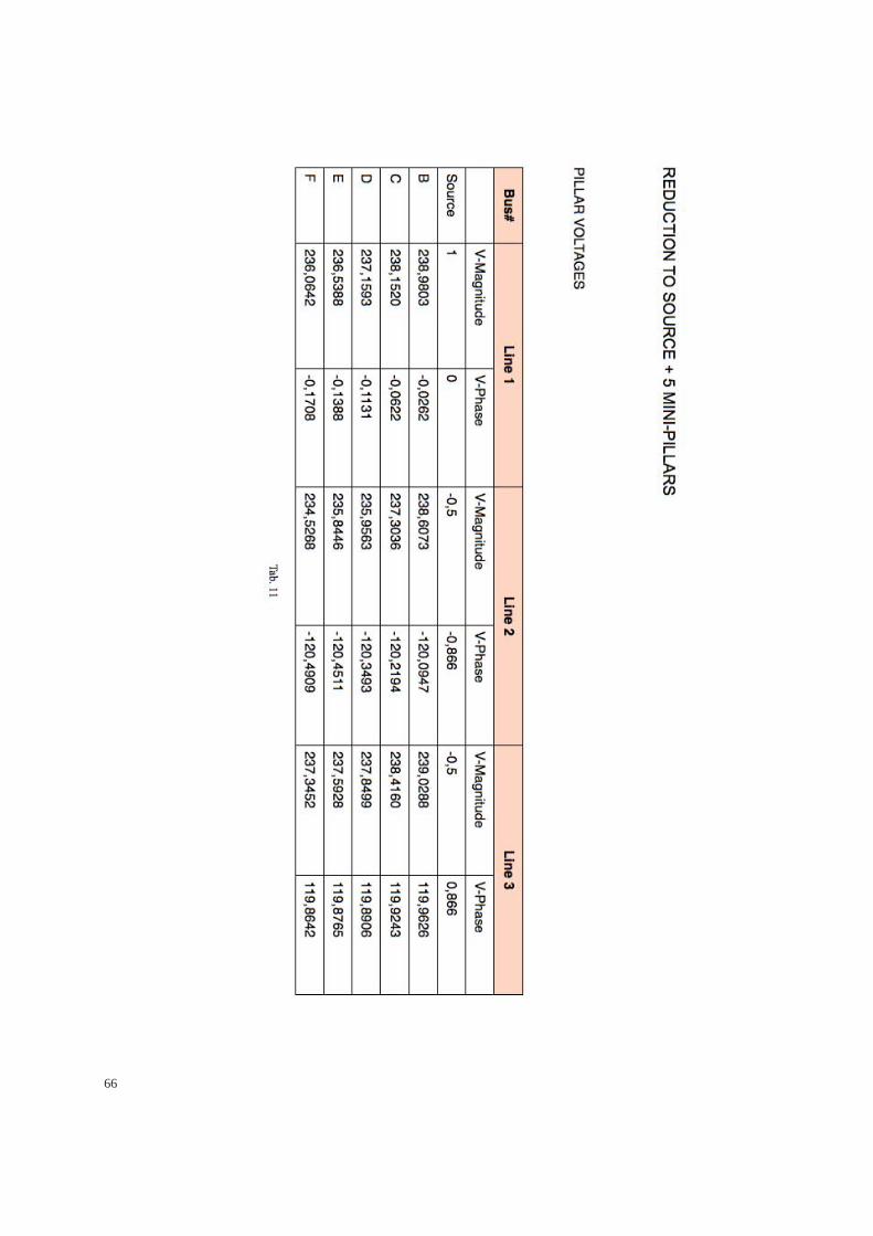
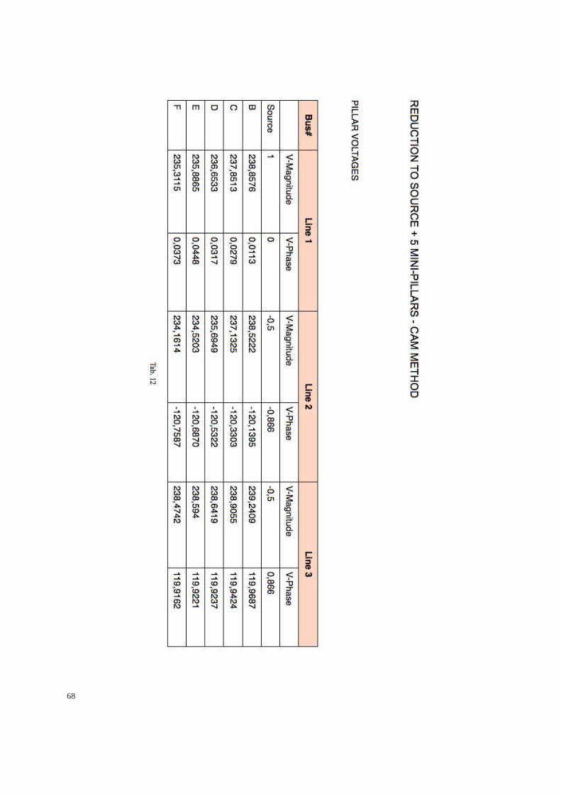
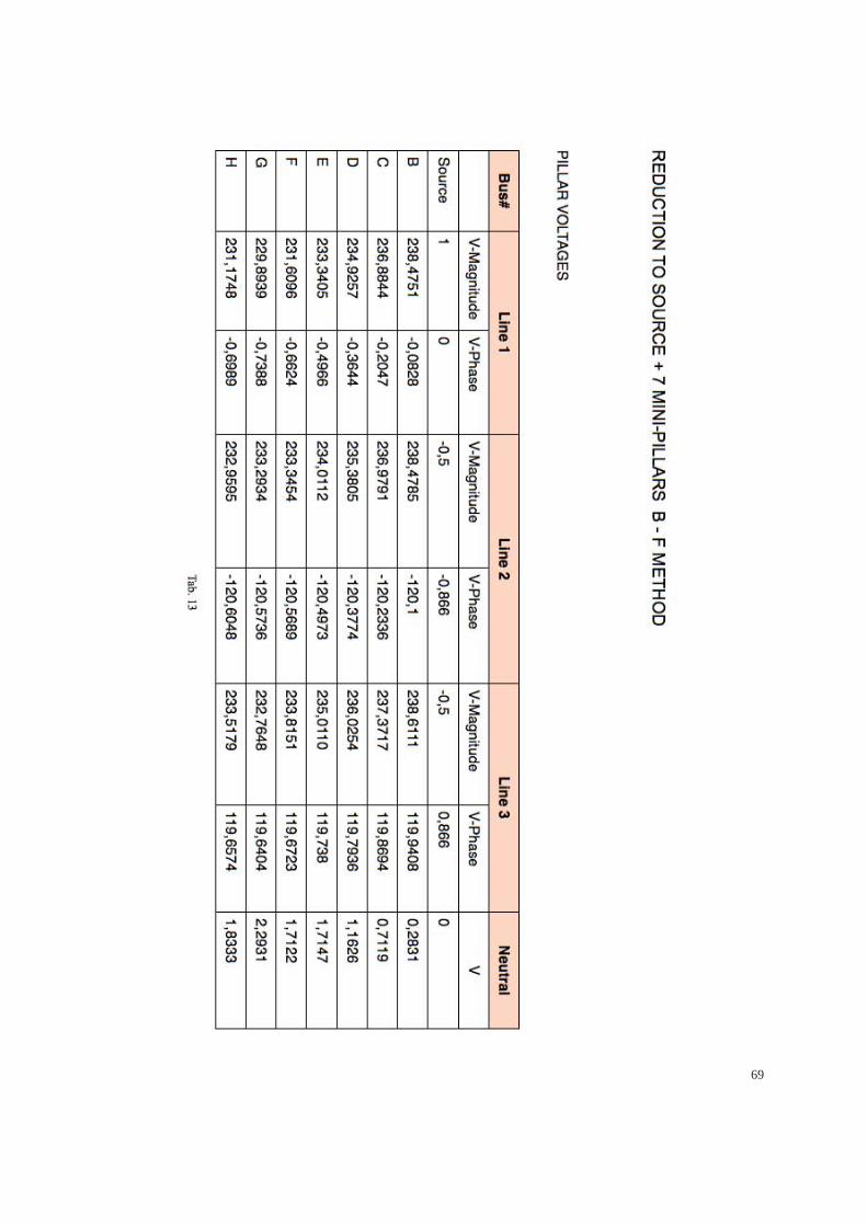
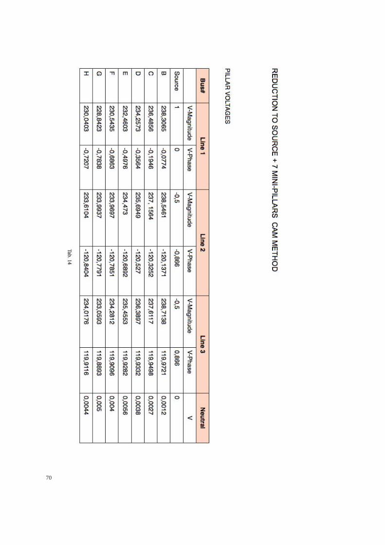
Smaller networks of 5 and 7 pillars are proposed for comparisons. In order to have
compatible results, the earth connection for the backward-forward were not involved.
64
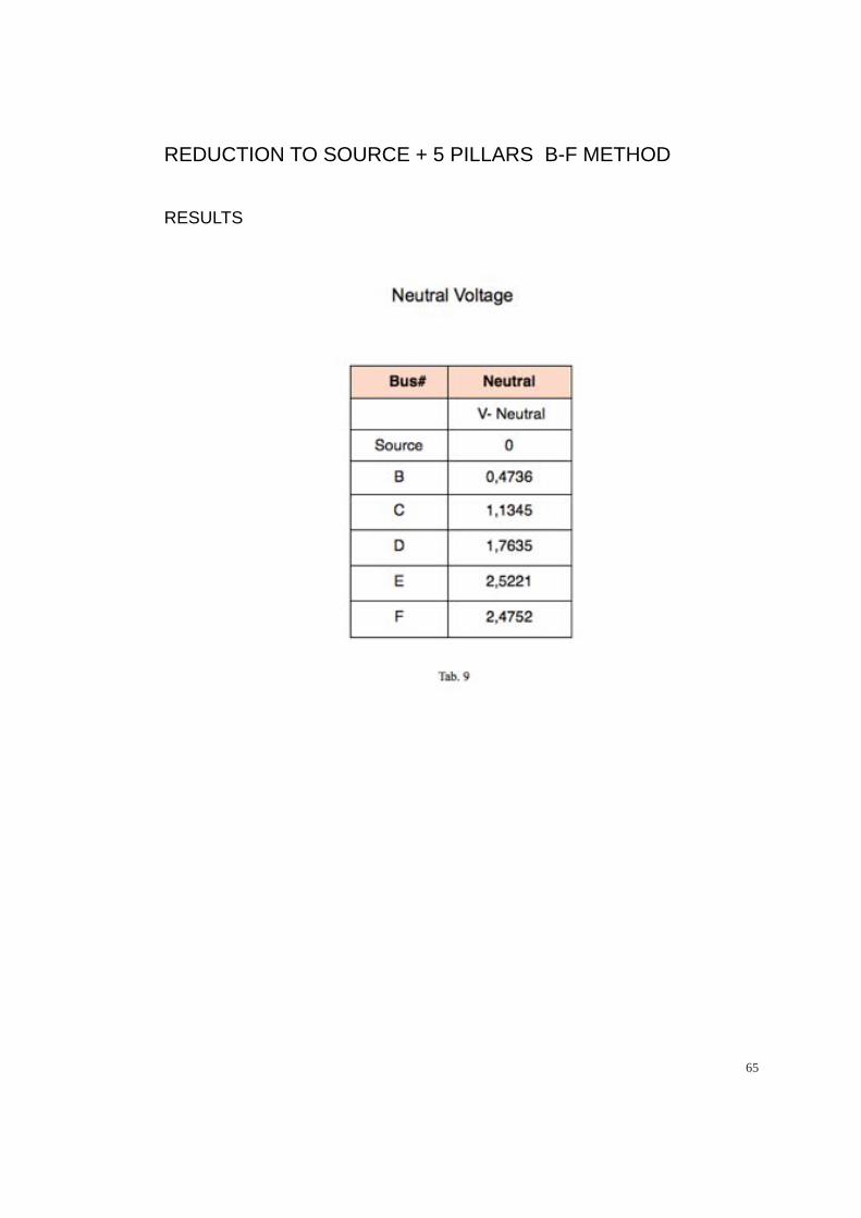
REDUCTION TO SOURCE + 5 PILLARS B-F METHOD
RESULTS
65
66

REDUCTION TO SOURCE + 5 MINI-PILLARS - CAM METHOD
RESULTS
67
68
69
70

71

Appendix ABackward-forward Method
Model_Entire_Network
clear allclose allclc%%%%%%%%%%%%%%%%%%%%%%%%%%%%%%%%%%%%%%%%%%%%%%%%%%%%%%%%%%%%%%%%%%%%%%%%%%%%%%%%%%%%%%%%%%%%%%%%%%%%%%%%%%%%%%%%%%%%%%%%%%%%%%%%%%%%%%%%%%%%%%%%%%%%%%% SYSTEM PARAMETERSV_line = 415;Sys_MVA_base = 1e+6;z_base = V_line^2/(Sys_MVA_base);% Earth Electrode(s)R_Pillar_Electrode=1/z_base;R_cons_electrode=10/z_base; System_Z; % Defining the system impedance network%%%%%%%%%%%%%%%%%%%%%%%%%%%%%%%%%%%%%%%%%%%%%%%%%%%%%%%%%%%%%%%%%%%%%%%%%%%%-------------------------------------------------------------------------%%Initialisation%-------------------------------------------------------------------------%Initial_Voltage % Assigning the flat start to all system bussesCustomer_Load_No_EarthElectrode % Deriving the comsumer load based o the flat startBranch_Current % Evaluating the branch currents (incorporaig the pillar current Diff=zeros(4,1); %Using X3 as the means to ascertain voltage profile%%%%%%%%%%%%%%%%%%%%%%%%%%%%%%%%%%%%%%%%%%%%%%%%%%%%%%%%%%%%%%%%%%%%%%%%%%%%-------------------------------------------------------------------------%%Load Flow Loop - Solution without Consumer Earth Electrodes%-------------------------------------------------------------------------% for i=1:400072
V_Diff=V_5; i % Convergnce parameter Voltage_Update if max(abs(V_Diff-V_5))<0.00001 % Convergence criteria break end Customer_Load_No_EarthElectrode % Deriving the comsumer load based o the flat start Branch_Current % Evaluating the branch currents (incorporaig the pillar current V_5 end %%%%%%%%%%%%%%%%%%%%%%%%%%%%%%%%%%%%%%%%%%%%%%%%%%%%%%%%%%%%%%%%%%%%%%%%%%%%-------------------------------------------------------------------------%%Load Flow Loop - Addition of Consumer Earth Electrodes%-------------------------------------------------------------------------%for ii=1:4000 V_Diff=V_5; iiVoltage_Update if max(abs(V_Diff-V_5))<0.00001 break endCustomer_Load_With_EarthElectrodeBranch_CurrentV_5 end%%%%%%%%%%%%%%%%%%%%%%%%%%%%%%%%%%%%%%%%%%%%%%%%%%%%%%%%%%%%%%%%%%%%%%%%%%%A=[V2_unbalance V3_unbalance V4_unbalance V5_unbalance V6_unbalance V7_unbalance V8_unbalance V9_unbalance V10_unbalance]*100;A' RESULTS%%%%%%%%%%%%%%%%%%%%%%%%%%%%%%%%%%%%%%%%%%%%%%%%%%%%%%%%%%%%%%%%%%%%%%%%%%%
Initial_Voltage
V_ground=0;V_neutral=0; V=[(1+0i);(1*exp(-j*120*pi/180));(1*exp(-j*240*pi/180));V_neutral]; % in pu V_1=V; V_2=V; V_120=V; V_26=V; V_59=V; V_75=V; V_63=V; V_46=V; V_3=V; V_27=V; V_28=V; V_32=V; V_25=V; V_33=V; V_35=V; V_36=V;
73
Customer_Load_With_EarthElectrode
% Node (Customer Load) Currents)%MINI-PILLAR A1bus=120; [S_120 IL_120]=Sys_Load(bus,V_120);bus=26; [S_26 IL_26]=Sys_Load(bus,V_26);bus=59; [S_59 IL_59]=Sys_Load(bus,V_59);bus=75; [S_75 IL_75]=Sys_Load(bus,V_75);bus=63; [S_63 IL_63]=Sys_Load(bus,V_63);bus=46; [S_46 IL_46]=Sys_Load(bus,V_46);%MINI-PILLAR A2bus=27; [S_27 IL_27]=Sys_Load(bus,V_27);bus=28; [S_28 IL_28]=Sys_Load(bus,V_28);bus=32; [S_32 IL_32]=Sys_Load(bus,V_32);bus=25; [S_25 IL_25]=Sys_Load(bus,V_25);bus=33; [S_33 IL_33]=Sys_Load(bus,V_33);bus=35; [S_35 IL_35]=Sys_Load(bus,V_35);bus=36; [S_36 IL_36]=Sys_Load(bus,V_36);%MINI-PILLAR A3bus=37; [S_37 IL_37]=Sys_Load(bus,V_37);bus=34; [S_34 IL_34]=Sys_Load(bus,V_34);bus=39; [S_39 IL_39]=Sys_Load(bus,V_39);bus=48; [S_48 IL_48]=Sys_Load(bus,V_48);bus=41; [S_41 IL_41]=Sys_Load(bus,V_41);bus=49; [S_49 IL_49]=Sys_Load(bus,V_49);bus=72; [S_72 IL_72]=Sys_Load(bus,V_72);bus=67; [S_67 IL_67]=Sys_Load(bus,V_67);bus=64; [S_64 IL_64]=Sys_Load(bus,V_64);%MINI-PILLAR A4bus=47; [S_47 IL_47]=Sys_Load(bus,V_47);bus=38; [S_38 IL_38]=Sys_Load(bus,V_38);bus=61; [S_61 IL_61]=Sys_Load(bus,V_61);bus=50; [S_50 IL_50]=Sys_Load(bus,V_50);bus=56; [S_56 IL_56]=Sys_Load(bus,V_56);bus=40; [S_40 IL_40]=Sys_Load(bus,V_40);bus=44; [S_44 IL_44]=Sys_Load(bus,V_44);%MINI-PILLAR A5bus=62; [S_62 IL_62]=Sys_Load(bus,V_62);bus=45; [S_45 IL_45]=Sys_Load(bus,V_45);bus=58; [S_58 IL_58]=Sys_Load(bus,V_58);bus=57; [S_57 IL_57]=Sys_Load(bus,V_57);bus=53; [S_53 IL_53]=Sys_Load(bus,V_53);bus=60; [S_60 IL_60]=Sys_Load(bus,V_60);bus=43; [S_43 IL_43]=Sys_Load(bus,V_43);bus=52; [S_52 IL_52]=Sys_Load(bus,V_52);%MINI-PILLAR A5abus=71; [S_71 IL_71]=Sys_Load(bus,V_71);bus=79; [S_79 IL_79]=Sys_Load(bus,V_79);bus=77; [S_77 IL_77]=Sys_Load(bus,V_77);bus=76; [S_76 IL_76]=Sys_Load(bus,V_76);74
bus=73; [S_73 IL_73]=Sys_Load(bus,V_73);bus=68; [S_68 IL_68]=Sys_Load(bus,V_68);bus=69; [S_69 IL_69]=Sys_Load(bus,V_69);bus=78; [S_78 IL_78]=Sys_Load(bus,V_78);bus=70; [S_70 IL_70]=Sys_Load(bus,V_70);%MINI-PILLAR A6bus=55; [S_55 IL_55]=Sys_Load(bus,V_55);bus=74; [S_74 IL_74]=Sys_Load(bus,V_74);bus=54; [S_54 IL_54]=Sys_Load(bus,V_54);bus=42; [S_42 IL_42]=Sys_Load(bus,V_42);bus=51; [S_51 IL_51]=Sys_Load(bus,V_51);bus=65; [S_65 IL_65]=Sys_Load(bus,V_65);bus=66; [S_66 IL_66]=Sys_Load(bus,V_66);bus=1326; [S_1326 IL_1326]=Sys_Load(bus,V_1326);%MINI-PILLAR X2bus=166; [S_166 IL_166]=Sys_Load(bus,V_166);bus=165; [S_165 IL_165]=Sys_Load(bus,V_165);bus=168; [S_168 IL_168]=Sys_Load(bus,V_168);bus=162; [S_162 IL_162]=Sys_Load(bus,V_162);bus=167; [S_167 IL_167]=Sys_Load(bus,V_167);bus=164; [S_164 IL_164]=Sys_Load(bus,V_164);bus=173; [S_173 IL_173]=Sys_Load(bus,V_173);bus=169; [S_169 IL_169]=Sys_Load(bus,V_169);bus=156; [S_156 IL_156]=Sys_Load(bus,V_156);bus=171; [S_171 IL_171]=Sys_Load(bus,V_171);%MINI-PILLAR X3bus=159; [S_159 IL_159]=Sys_Load(bus,V_159);bus=178; [S_178 IL_178]=Sys_Load(bus,V_178);bus=177; [S_177 IL_177]=Sys_Load(bus,V_177);bus=179; [S_179 IL_179]=Sys_Load(bus,V_179);bus=176; [S_176 IL_176]=Sys_Load(bus,V_176);bus=163; [S_163 IL_163]=Sys_Load(bus,V_163);bus=161; [S_161 IL_161]=Sys_Load(bus,V_161);bus=172; [S_172 IL_172]=Sys_Load(bus,V_172);bus=175; [S_175 IL_175]=Sys_Load(bus,V_175);bus=174; [S_174 IL_174]=Sys_Load(bus,V_174);
Sys_Load
function [Sabc, Iabcng]= Sys_Load(bus, V) bus;Sys_MVA_base = 1e+6;load Load.txtLoad(:,[2:7])=(Load(:,[2:7])*1000)/(Sys_MVA_base/3); %Load(:,1) = = Bus ID %Load(:,2) = = P_L1 %Load(:,3) = = Q_L1 %Load(:,4) = = P_L2 %Load(:,5) = = Q_L2 %Load(:,6) = = P_L3 %Load(:,7) = = Q_L3
75
row=Load(:,1);for i=1:length(Load(:,1)); loc(i)=row(i)-bus; endpos=find(loc==0);row_ID=pos(1,1); Sabc=[Load(row_ID,2)+j*Load(row_ID,3) Load(row_ID,4)+j*Load(row_ID,5) Load(row_ID,6)+j*Load(row_ID,7)];% V(4)% pauseIa=conj(Sabc(1))./(conj(V(1)-V(4)));Ib=conj(Sabc(2))./(conj(V(2)-V(4)));Ic=conj(Sabc(3))./(conj(V(3)-V(4)));%pause Rcons=.15; In=-(Ia+Ib+Ic)+(V(4))/Rcons;%-Ig %pauseIabcng=[Ia;Ib;Ic;In;];%pause Branch_Current
%Pillar X3Pillar=9; I_174=IL_174;I_175=IL_175;I_172=IL_172;I_161=IL_161;I_163=IL_163;I_176=IL_176;I_179=IL_179;I_177=IL_177;I_178=IL_178;I_159=IL_159; I_10=I_174+I_175+I_172+I_161+I_163+I_176+I_179+I_177+I_178+I_159; %pause I=I_10; Rg_pillar=R_Pillar_Electrode; [I_Pillar]= Pillar_Current(Pillar,I,V_10,Rg_pillar); I_10=I_Pillar;%Pillar X2 Pillar=8; I_171=IL_171;I_156=IL_156;I_169=IL_169;I_173=IL_173;I_164=IL_164;I_167=IL_167;I_162=IL_162;I_168=IL_168;I_165=IL_165;I_166=IL_166; I_9=I_171+I_156+I_169+I_173+I_164+I_167+I_162+I_168+I_165+I_166+I_10; I=I_9; Rg_pillar=R_Pillar_Electrode; [I_Pillar]= Pillar_Current(Pillar,I,V_9,Rg_pillar); I_9=I_Pillar; 76

%Pillar A6 Pillar=7; I_1326=IL_1326;I_66=IL_66;I_65=IL_65;I_51=IL_51;I_42=IL_42;I_54=IL_54;I_74=IL_74;I_55=IL_55; I_8=I_1326+I_66+I_65+I_51+I_42+I_54+I_74+I_55+I_9; I=I_8; Rg_pillar=R_Pillar_Electrode; [I_Pillar]= Pillar_Current(Pillar,I,V_8,Rg_pillar); I_8=I_Pillar; %Pillar A5a Pillar=6; I_70=IL_70;I_78=IL_78;I_69=IL_69;I_68=IL_68;I_73=IL_73;I_76=IL_76;I_77=IL_77;I_79=IL_79;I_71=IL_71; I_7=I_70+I_78+I_69+I_68+I_73+I_76+I_77+I_79+I_71; I=I_7; Rg_pillar=R_Pillar_Electrode; [I_Pillar]= Pillar_Current(Pillar,I,V_7,Rg_pillar); I_7=I_Pillar; %Pillar A5 Pillar=5; I_62=IL_62;I_45=IL_45;I_58=IL_58;I_57=IL_57;I_53=IL_53;I_60=IL_60;I_43=IL_43;I_52=IL_52; I_6=I_62+I_45+I_58+I_57+I_53+I_60+I_43+I_52+I_7+I_8; I=I_6; Rg_pillar=R_Pillar_Electrode; [I_Pillar]= Pillar_Current(Pillar,I,V_6,Rg_pillar); I_6=I_Pillar; %Pillar A4 Pillar=4; I_47=IL_47;I_38=IL_38;I_61=IL_61;I_50=IL_50;I_56=IL_56;I_40=IL_40;I_44=IL_44; I_5=I_47+I_38+I_61+I_50+I_56+I_40+I_44+I_6; I=I_5; Rg_pillar=R_Pillar_Electrode; [I_Pillar]= Pillar_Current(Pillar,I,V_5,Rg_pillar); I_5=I_Pillar; %Pillar A3 Pillar=3; I_64=IL_64;I_67=IL_67;I_72=IL_72;I_49=IL_49;I_41=IL_41;I_48=IL_48;I_39=IL_39;I_34=IL_34;I_37=IL_37; I_4=I_64+I_67+I_72+I_49+I_41+I_48+I_39+I_34+I_37+I_5; I=I_4; Rg_pillar=R_Pillar_Electrode; [I_Pillar]= Pillar_Current(Pillar,I,V_4,Rg_pillar); I_4=I_Pillar;%Pillar A2 Pillar=2; I_36=IL_36;I_35=IL_35;I_33=IL_33;I_25=IL_25;I_32=IL_32;I_27=IL_27;I_28=IL_28; I_3=I_36+I_35+I_33+I_25+I_32+I_27+I_28+I_4; I=I_3; Rg_pillar=R_Pillar_Electrode; [I_Pillar]= Pillar_Current(Pillar,I,V_3,Rg_pillar); I_3=I_Pillar; %Pillar A1 Pillar=1; I_46=IL_46;I_63=IL_63;I_75=IL_75;I_59=IL_59;I_26=IL_26;I_120=IL_120; I_2=I_46+I_63+I_75+I_59+I_26+I_120+I_3;
77
I=I_2; Rg_pillar=R_Pillar_Electrode; [I_Pillar]= Pillar_Current(Pillar,I,V_2,Rg_pillar); I_2=I_Pillar; % SUBSTATION - A I_1=I_2;
Pillar_Current
function [I_Pillar]= Pillar_Current(Pillar, I,V,Rg_pillar) Pillar; % In=I(4)-(V(4)-V(5))/Rg_pillar; % Modified KS (020912)% Ig=I(5)+(V(4)-V(5))/Rg_pillar; % Modified KS (020912) In=I(4)+(V(4))/Rg_pillar; % MC I_Pillar=[I(1);I(2); I(3); In;]; %pause %sum(I_Pillar); %pause end
Voltage_Update
%-------- SOURCE ---------%ZE=0.00001;IE=-(I_1(1)+I_1(2)+I_1(3)+I_1(4));V_1(4)=V_1(4)+IE*ZE;V_1=[(1+0i)+V_1(4);(1*exp(-j*120*pi/180))+V_1(4);(1*exp(-j*240*pi/180))+V_1(4);V_1(4)]; % in pu %-------- Mini-pillar A1 ---------%V_2=(V_1-(z_A_A1*I_2));[V2_unbalance]=Voltage_Unbalance(V_2); V_120=V_2-(z_A1_C120*I_120); V_26=V_2-(z_A1_C26*I_26); V_59=V_2-(z_A1_C59*I_59); V_75=V_2-(z_A1_C75*I_75); V_63=V_2-(z_A1_C63*I_63); V_46=V_2-(z_A1_C46*I_46);%-------- Mini-pillar A2 ---------% V_3=(V_2-(z_A1_A2*I_3));
78
Diff;% pause[V3_unbalance]=Voltage_Unbalance(V_3); V_36=V_3-(z_A2_C36*I_36); V_35=V_3-(z_A2_C35*I_35); V_33=V_3-(z_A2_C33*I_33); V_25=V_3-(z_A2_C25*I_25); V_32=V_3-(z_A2_C32*I_32); V_27=V_3-(z_A2_C27*I_27); V_28=V_3-(z_A2_C28*I_28);%-------- Mini-pillar A3 ---------%V_4=(V_3-(z_A2_A3*I_4));[V4_unbalance]=Voltage_Unbalance(V_4); V_41=V_4-(z_A3_C41*I_41); V_48=V_4-(z_A3_C48*I_48); V_39=V_4-(z_A3_C39*I_39); V_34=V_4-(z_A3_C34*I_34); V_37=V_4-(z_A3_C37*I_37); V_64=V_4-(z_A3_C64*I_64); V_67=V_4-(z_A3_C67*I_67); V_72=V_4-(z_A3_C72*I_72); V_49=V_4-(z_A3_C49*I_49); %-------- Mini-pillar A4 ---------%V_5=(V_4-(z_A3_A4*I_5));[V5_unbalance]=Voltage_Unbalance(V_5); V_47=V_5-(z_A4_C47*I_47); V_38=V_5-(z_A4_C38*I_38); V_61=V_5-(z_A4_C61*I_61); V_50=V_5-(z_A4_C50*I_50); V_56=V_5-(z_A4_C56*I_56); V_40=V_5-(z_A4_C40*I_40); V_44=V_5-(z_A4_C44*I_44); %-------- Mini-pillar A5 ---------%V_6=(V_5-(z_A4_A5*I_6));[V6_unbalance]=Voltage_Unbalance(V_6); V_62=V_6-(z_A5_C62*I_62); V_45=V_6-(z_A5_C45*I_45); V_58=V_6-(z_A5_C58*I_58); V_57=V_6-(z_A5_C57*I_57); V_53=V_6-(z_A5_C53*I_53); V_60=V_6-(z_A5_C60*I_60); V_43=V_6-(z_A5_C43*I_43); V_52=V_6-(z_A5_C52*I_52); %-------- Mini-pillar A5a ---------%V_7=(V_6-(z_A5_A5a*I_7));[V7_unbalance]=Voltage_Unbalance(V_7); V_71=V_7-(z_A5a_C71*I_71); V_79=V_7-(z_A5a_C79*I_79); V_77=V_7-(z_A5a_C77*I_77);
79
V_76=V_7-(z_A5a_C76*I_76); V_73=V_7-(z_A5a_C73*I_73); V_68=V_7-(z_A5a_C68*I_68); V_69=V_7-(z_A5a_C69*I_69); V_78=V_7-(z_A5a_C78*I_78); V_70=V_7-(z_A5a_C70*I_70); %-------- Mini-pillar A6 ---------%V_8=(V_6-(z_A5_A6*I_8));[V8_unbalance]=Voltage_Unbalance(V_8); V_1326=V_8-(z_A6_C1326*I_1326); V_66=V_8-(z_A6_C66*I_66); V_65=V_8-(z_A6_C65*I_65); V_51=V_8-(z_A6_C51*I_51); V_42=V_8-(z_A6_C42*I_42); V_54=V_8-(z_A6_C54*I_54); V_74=V_8-(z_A6_C74*I_74); V_55=V_8-(z_A6_C55*I_55); %-------- Mini-pillar X2 ---------%V_9=(V_8-(z_A6_X2*I_9));[V9_unbalance]=Voltage_Unbalance(V_9); V_164=V_9-(z_X2_C164*I_164); V_173=V_9-(z_X2_C173*I_173); V_169=V_9-(z_X2_C169*I_169); V_156=V_9-(z_X2_C156*I_156); V_171=V_9-(z_X2_C171*I_171); V_166=V_9-(z_X2_C166*I_166); V_165=V_9-(z_X2_C165*I_165); V_168=V_9-(z_X2_C168*I_168); V_162=V_9-(z_X2_C162*I_162); V_167=V_9-(z_X2_C167*I_167); %-------- Mini-pillar X3 ---------%V_10=(V_9-(z_X2_X3*I_9));[V10_unbalance]=Voltage_Unbalance(V_10); V_163=V_10-(z_X3_C163*I_1326); V_161=V_10-(z_X3_C161*I_161); V_172=V_10-(z_X3_C172*I_172); V_175=V_10-(z_X3_C175*I_175); V_174=V_10-(z_X3_C174*I_174); V_159=V_10-(z_X3_C159*I_159); V_178=V_10-(z_X3_C178*I_178); V_177=V_10-(z_X3_C177*I_177); V_179=V_10-(z_X3_C179*I_179); V_176=V_10-(z_X3_C176*I_176);
80

Z_Branch
% K. Sunderland% 10th October, 2012%0000000000000000000000000000000000000000000000000000000000000000000000000% function Zabcng= Z_Branch(c_length, line_config) % needs to be converted to ''per-miles %%%%%%%%%%%%%%%%%%%%%%%%%%%%%%%%%%%%%%%%%%%%%%%%%%%%%%%%%%%%%%%%%%%%%%%%%%% %----------------------------- CONSTANTS ---------------------------------%f=50;V_line = 415;Sys_MVA_base = 1e+6;z_base = V_line^2/(Sys_MVA_base);rho=100;%-------------------------------------------------------------------------% %%%%%%%%%%%%%%%%%%%%%%%%%%%%%%%%%%%%%%%%%%%%%%%%%%%%%%%%%%%%%%%%%%%%%%%%%%%%%%%%%%%%%%%%%%%%%%%%%%%%%%%%%%%%%%%%%%%%%%%%%%%%%%%%%%%%%%%%%%%%%%%%%%%%%% if line_config == 1 % 1 == 70-XLPE [TEST 3-phase Cable (as per Ciric paper)]f=50;rho=100;ri_line=0.569;Rad_con=0.01025/2;GMR_line=0.7788*Rad_con; ri_n=0.569;GMR_n=0.7788*Rad_con; %% GEOMETRIC DISTANCES %%%Geometric spacing of the f-core cablea=[0,0];b=[0.0109,0];c=[0,-0.0109];n=[0.0109, -0.0109]; % Cable HeightDepth 1m (Not sure if this is a plausible depth)
81
%-------------------------------------------------------------------------%ha=2.00-0.00545; % Heights/Depths based on dimensions derived in 'UG XLPE.doc'hb=2.00-0.00545;hc=2.00+0.00545;hn=2.00+0.00545; %Conductor Horizontal Distrances%-------------------------------------------------------------------------%dab=10.9/1000; dac=0;dan=10.9/1000;dba=dab; dbc=10.9/1000; dbn=0;dca=dac; dcb=dbc; dcn=10.9/1000;dna=dan; dnb=dbn; dnc=dcn; %-------------------------------------------------------------------------%%% DEFINING THE PRIMITIVE (partitioned) Z-MATRIX %%zaa=(ri_line+j*4*pi*(10^-4)*f*(log((2*ha)/GMR_line)));zbb=(ri_line+j*4*pi*(10^-4)*f*(log((2*hb)/GMR_line)));zcc=(ri_line+j*4*pi*(10^-4)*f*(log((2*hc)/GMR_line)));znn=(ri_n+j*4*pi*(10^-4)*f*(log((2*hn)/GMR_n))); zab=j*4*pi*(10^-4)*f*log((sqrt(dab^2+(ha+hb)^2))/(sqrt(dab^2+(ha-hb)^2)));zac=j*4*pi*(10^-4)*f*log((sqrt(dac^2+(ha+hc)^2))/(sqrt(dac^2+(ha-hc)^2)));zan=j*4*pi*(10^-4)*f*log((sqrt(dan^2+(ha+hn)^2))/(sqrt(dan^2+(ha-hn)^2)));zna=zan;zba=zab;zbc=j*4*pi*(10^-4)*f*log((sqrt(dbc^2+(hb+hc)^2))/(sqrt(dbc^2+(hb-hc)^2)));zbn=j*4*pi*(10^-4)*f*log((sqrt(dbn^2+(hb+hn)^2))/(sqrt(dbn^2+(hb-hn)^2)));znb=zbn;zca=zac;zcb=zbc;zcn=j*4*pi*(10^-4)*f*log((sqrt(dcn^2+(hc+hn)^2))/(sqrt(dcn^2+(hc-hn)^2)));znc=zcn;% %-------------------------------------------------------------------------% %% Primitive Matrix %%Zabcng=[zaa zab zac zan; zba zbb zbc zbn; zca zcb zcc zcn; zna znb znc znn;]*(c_length/1000);
82

end%%%%%%%%%%%%%%%%%%%%%%%%%%%%%%%%%%%%%%%%%%%%%%%%%%%%%%%%%%%%%%%%%%%%%%%%%%%%%%%%%%%%%%%%%%%%%%%%%%%%%%%%%%%%%%%%%%%%%%%%%%%%%%%%%%%%%%%%%%%%%%%%%%%%%%if line_config == 2 % 2 == 185-XLPE [TEST 3-phase Cable (as per Ciric paper)]f=50;rho=100;ri_line=0.212;Rad_con=0.01573/2;GMR_line=0.7788*Rad_con;ri_n=0.212;GMR_n=0.7788*Rad_con; %% GEOMETRIC DISTANCES %%%Geometric spacing of the f-core cablea=[0,0];b=[0.01655,0];c=[0,-0.01655];n=[0.01655,-0.01655]; % Cable HeightDepth 1m (Not sure if this is a plausible depth)%-------------------------------------------------------------------------%ha=2.00-0.008275; % Heights based on dimensions derived in 'UG XLPE.doc'hb=2.00-0.008275;hc=2.00+0.008275;hn=2.00+0.008275; %Conductor Horizontal Distrances%-------------------------------------------------------------------------%dab=0.01655; dac=0;dan=0.01655;dba=dab; dbc=0.01655; dbn=0;dca=dac; dcb=dbc; dcn=0.01655;dna=dan; dnb=dbn; dnc=dcn; %-------------------------------------------------------------------------%%% DEFINING THE PRIMITIVE (partitioned) Z-MATRIX %%zaa=(ri_line+j*4*pi*(10^-4)*f*(log((2*ha)/GMR_line)));zbb=(ri_line+j*4*pi*(10^-4)*f*(log((2*hb)/GMR_line)));zcc=(ri_line+j*4*pi*(10^-4)*f*(log((2*hc)/GMR_line)));znn=(ri_n+j*4*pi*(10^-4)*f*(log((2*hn)/GMR_n)));
83

zab=j*4*pi*(10^-4)*f*log((sqrt(dab^2+(ha+hb)^2))/(sqrt(dab^2+(ha-hb)^2)));zac=j*4*pi*(10^-4)*f*log((sqrt(dac^2+(ha+hc)^2))/(sqrt(dac^2+(ha-hc)^2)));zan=j*4*pi*(10^-4)*f*log((sqrt(dan^2+(ha+hn)^2))/(sqrt(dan^2+(ha-hn)^2)));zna=zan;zba=zab;zbc=j*4*pi*(10^-4)*f*log((sqrt(dbc^2+(hb+hc)^2))/(sqrt(dbc^2+(hb-hc)^2)));zbn=j*4*pi*(10^-4)*f*log((sqrt(dbn^2+(hb+hn)^2))/(sqrt(dbn^2+(hb-hn)^2)));znb=zbn;zca=zac;zcb=zbc;zcn=j*4*pi*(10^-4)*f*log((sqrt(dcn^2+(hc+hn)^2))/(sqrt(dcn^2+(hc-hn)^2)));znc=zcn; % %-------------------------------------------------------------------------% %% Primitive Matrix %%Zabcng=[zaa zab zac zan; zba zbb zbc zbn; zca zcb zcc zcn; zna znb znc znn;]*(c_length/1000); end%%%%%%%%%%%%%%%%%%%%%%%%%%%%%%%%%%%%%%%%%%%%%%%%%%%%%%%%%%%%%%%%%%%%%%%%%%%%%%%%%%%%%%%%%%%%%%%%%%%%%%%%%%%%%%%%%%%%%%%%%%%%%%%%%%%%%%%%%%%%%%%%%%%%%%if line_config == 3 % 3 == 70-NAKBA [TEST 3-phase Cable (as per Ciric paper)]f=50;rho=100;ri_line=0.507;Rad_con=0.00986/2;GMR_line=0.7788*Rad_con;ri_n=0.507;GMR_n=0.7788*Rad_con; %% GEOMETRIC DISTANCES %%%Geometric spacing of the f-core cablea=[0,0];b=[0.0107,0];c=[0,-0.0107];n=[0.0107,-0.0107];
84
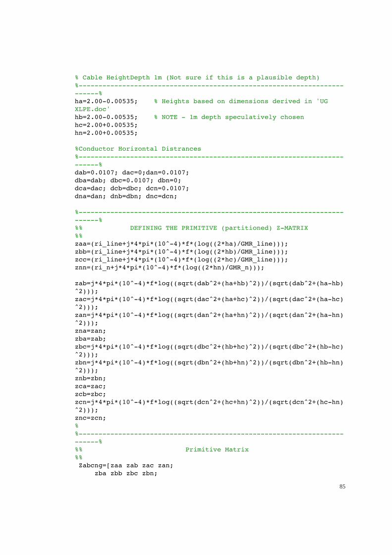
% Cable HeightDepth 1m (Not sure if this is a plausible depth)%-------------------------------------------------------------------------%ha=2.00-0.00535; % Heights based on dimensions derived in 'UG XLPE.doc' hb=2.00-0.00535; % NOTE - 1m depth speculatively chosenhc=2.00+0.00535;hn=2.00+0.00535; %Conductor Horizontal Distrances%-------------------------------------------------------------------------%dab=0.0107; dac=0;dan=0.0107;dba=dab; dbc=0.0107; dbn=0;dca=dac; dcb=dbc; dcn=0.0107;dna=dan; dnb=dbn; dnc=dcn; %-------------------------------------------------------------------------%%% DEFINING THE PRIMITIVE (partitioned) Z-MATRIX %%zaa=(ri_line+j*4*pi*(10^-4)*f*(log((2*ha)/GMR_line)));zbb=(ri_line+j*4*pi*(10^-4)*f*(log((2*hb)/GMR_line)));zcc=(ri_line+j*4*pi*(10^-4)*f*(log((2*hc)/GMR_line)));znn=(ri_n+j*4*pi*(10^-4)*f*(log((2*hn)/GMR_n))); zab=j*4*pi*(10^-4)*f*log((sqrt(dab^2+(ha+hb)^2))/(sqrt(dab^2+(ha-hb)^2)));zac=j*4*pi*(10^-4)*f*log((sqrt(dac^2+(ha+hc)^2))/(sqrt(dac^2+(ha-hc)^2)));zan=j*4*pi*(10^-4)*f*log((sqrt(dan^2+(ha+hn)^2))/(sqrt(dan^2+(ha-hn)^2)));zna=zan;zba=zab;zbc=j*4*pi*(10^-4)*f*log((sqrt(dbc^2+(hb+hc)^2))/(sqrt(dbc^2+(hb-hc)^2)));zbn=j*4*pi*(10^-4)*f*log((sqrt(dbn^2+(hb+hn)^2))/(sqrt(dbn^2+(hb-hn)^2)));znb=zbn;zca=zac;zcb=zbc;zcn=j*4*pi*(10^-4)*f*log((sqrt(dcn^2+(hc+hn)^2))/(sqrt(dcn^2+(hc-hn)^2)));znc=zcn;% %-------------------------------------------------------------------------% %% Primitive Matrix %% Zabcng=[zaa zab zac zan; zba zbb zbc zbn;
85
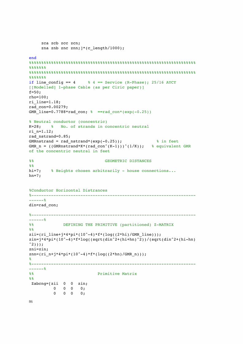
zca zcb zcc zcn; zna znb znc znn;]*(c_length/1000); end%%%%%%%%%%%%%%%%%%%%%%%%%%%%%%%%%%%%%%%%%%%%%%%%%%%%%%%%%%%%%%%%%%%%%%%%%%%%%%%%%%%%%%%%%%%%%%%%%%%%%%%%%%%%%%%%%%%%%%%%%%%%%%%%%%%%%%%%%%%%%%%%%%%%%%if line_config == 4 % 4 == Service (R-Phase); 25/16 AYCY [[Modelled] 1-phase Cable (as per Ciric paper)]f=50;rho=100;ri_line=1.18;rad_con=0.00279;GMR_line=0.7788*rad_con; % ==rad_con*(exp(-0.25)) % Neutral conductor (concentric)K=28; % No. of strands in concentric neutralri_n=1.12;rad_nstrand=0.85; GMRnstrand = rad_nstrand*(exp(-0.25)); % in feetGMR_n = ((GMRnstrand*K*(rad_con^(K-1)))^(1/K)); % equivalent GMR of the concentric neutral in feet %% GEOMETRIC DISTANCES %%hi=7; % Heights chosen arbitrarily - house connections...hn=7; %Conductor Horizontal Distrances%-------------------------------------------------------------------------%din=rad_con; %-------------------------------------------------------------------------%%% DEFINING THE PRIMITIVE (partitioned) Z-MATRIX %%zii=(ri_line+j*4*pi*(10^-4)*f*(log((2*hi)/GMR_line)));zin=j*4*pi*(10^-4)*f*log((sqrt(din^2+(hi+hn)^2))/(sqrt(din^2+(hi-hn)^2)));zni=zin;znn=(ri_n+j*4*pi*(10^-4)*f*(log((2*hn)/GMR_n)));% %-------------------------------------------------------------------------% %% Primitive Matrix %% Zabcng=[zii 0 0 zin; 0 0 0 0; 0 0 0 0;
86
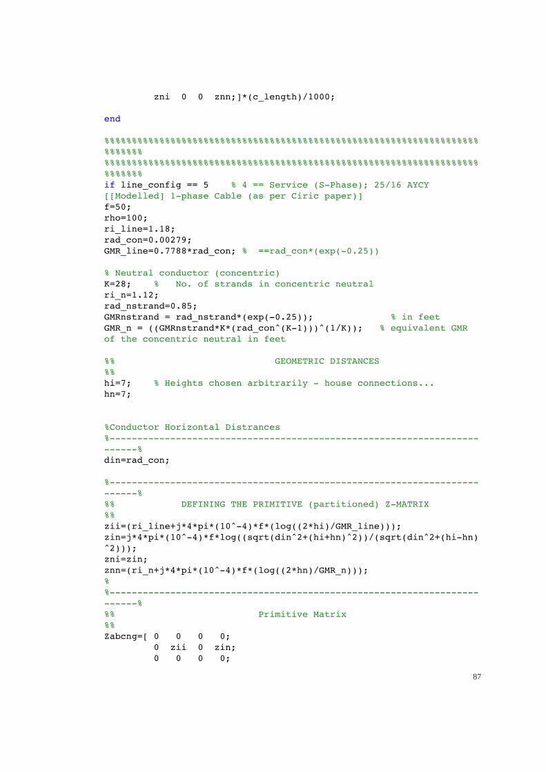
zni 0 0 znn;]*(c_length)/1000; end %%%%%%%%%%%%%%%%%%%%%%%%%%%%%%%%%%%%%%%%%%%%%%%%%%%%%%%%%%%%%%%%%%%%%%%%%%%%%%%%%%%%%%%%%%%%%%%%%%%%%%%%%%%%%%%%%%%%%%%%%%%%%%%%%%%%%%%%%%%%%%%%%%%%%%if line_config == 5 % 4 == Service (S-Phase); 25/16 AYCY [[Modelled] 1-phase Cable (as per Ciric paper)]f=50;rho=100;ri_line=1.18;rad_con=0.00279;GMR_line=0.7788*rad_con; % ==rad_con*(exp(-0.25)) % Neutral conductor (concentric)K=28; % No. of strands in concentric neutralri_n=1.12;rad_nstrand=0.85; GMRnstrand = rad_nstrand*(exp(-0.25)); % in feetGMR_n = ((GMRnstrand*K*(rad_con^(K-1)))^(1/K)); % equivalent GMR of the concentric neutral in feet %% GEOMETRIC DISTANCES %%hi=7; % Heights chosen arbitrarily - house connections...hn=7; %Conductor Horizontal Distrances%-------------------------------------------------------------------------%din=rad_con; %-------------------------------------------------------------------------%%% DEFINING THE PRIMITIVE (partitioned) Z-MATRIX %%zii=(ri_line+j*4*pi*(10^-4)*f*(log((2*hi)/GMR_line)));zin=j*4*pi*(10^-4)*f*log((sqrt(din^2+(hi+hn)^2))/(sqrt(din^2+(hi-hn)^2)));zni=zin;znn=(ri_n+j*4*pi*(10^-4)*f*(log((2*hn)/GMR_n)));% %-------------------------------------------------------------------------% %% Primitive Matrix %%Zabcng=[ 0 0 0 0; 0 zii 0 zin; 0 0 0 0;
87
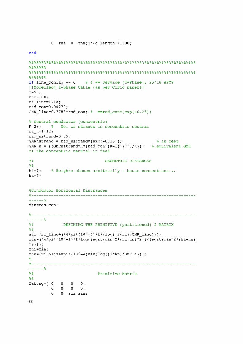
0 zni 0 znn;]*(c_length)/1000; end %%%%%%%%%%%%%%%%%%%%%%%%%%%%%%%%%%%%%%%%%%%%%%%%%%%%%%%%%%%%%%%%%%%%%%%%%%%%%%%%%%%%%%%%%%%%%%%%%%%%%%%%%%%%%%%%%%%%%%%%%%%%%%%%%%%%%%%%%%%%%%%%%%%%%%if line_config == 6 % 4 == Service (T-Phase); 25/16 AYCY [[Modelled] 1-phase Cable (as per Ciric paper)]f=50;rho=100;ri_line=1.18;rad_con=0.00279;GMR_line=0.7788*rad_con; % ==rad_con*(exp(-0.25)) % Neutral conductor (concentric)K=28; % No. of strands in concentric neutralri_n=1.12;rad_nstrand=0.85; GMRnstrand = rad_nstrand*(exp(-0.25)); % in feetGMR_n = ((GMRnstrand*K*(rad_con^(K-1)))^(1/K)); % equivalent GMR of the concentric neutral in feet %% GEOMETRIC DISTANCES %%hi=7; % Heights chosen arbitrarily - house connections...hn=7; %Conductor Horizontal Distrances%-------------------------------------------------------------------------%din=rad_con; %-------------------------------------------------------------------------%%% DEFINING THE PRIMITIVE (partitioned) Z-MATRIX %%zii=(ri_line+j*4*pi*(10^-4)*f*(log((2*hi)/GMR_line)));zin=j*4*pi*(10^-4)*f*log((sqrt(din^2+(hi+hn)^2))/(sqrt(din^2+(hi-hn)^2)));zni=zin;znn=(ri_n+j*4*pi*(10^-4)*f*(log((2*hn)/GMR_n)));% %-------------------------------------------------------------------------% %% Primitive Matrix %%Zabcng=[ 0 0 0 0; 0 0 0 0; 0 0 zii zin;
88

0 0 zni znn;]*(c_length)/1000; end
89

Appendix BMain_CAM
%%%%%%%%%%%%%%%%%%%%%%%%%%%%%%%%%%%%%%%%%%%%%%%%%%%%%%%%%%%%%%%%%%%%%%%%%%%------------------------------------------------------------------------%%% CAM Load Flow Solution %% %------------------------------------------------------------------------%%Supervisor: M. F. Conlon %Student: K. Sunderland%Dublin Institute of Technology%Date 10/02/13%%%%%%%%%%%%%%%%%%%%%%%%%%%%%%%%%%%%%%%%%%%%%%%%%%%%%%%%%%%%%%%%%%%%%%%%%% %Clear workspace and close any open filesclose allclear all% clc% Add the path to the following directories:path(1,1)={'\Calcs\'};path(2,1)={'\Data\'};for ni=1:size(path,1) addpath([pwd path{ni}]);end%%%%%%%%%%%%%%%%%%%%%%%%%%%%%%%%%%%%%%%%%%%%%%%%%%%%%%%%%%%%%%%%%%%%%%%%%% %------------------------- System Parameters -------------------------% V_line = 415/sqrt(3);V_neutral=0;V_flat=[(1+0i);(1*exp(-j*120*pi/180));(1*exp(-j*240*pi/180));V_neutral]; % in pu Sys_MVA_base = 1e+6;z_base = (V_line^2)/(Sys_MVA_base); %-----------------------------------------------------------------------% Four_Wire_Y_Sys; % Creating the 4-wire Y-bus network structure
90
Two_Wire_Y_Sys; % Accomodating the additional 2-wire line(s) to % the 4-wire (backbone) Y-matrix Earth_Elec; % Adding the Earth Electrode Resistance % (Cons. & Pillar) Sys_LF; % Accomodating the Load System Y-matrix & Sys. LF % Y(188,188) %%%%%%%%%%%%%%%%%%%%%%%%%%%%%%%%%%%%%%%%%%%%%%%%%%%%%%%%%%%%%%%%%%%%Results_outfor ni=1:nbranch_4wire*4-1 E_matrix(1:4,ni)=V_Sys((1:4)+4*(ni-1),1); end exp_results(E_matrix,(1:5),it,1);
Network
%Bus informations loadingfunction [i,fb, tb, line_config,c_length, Y_Load]=Network(Wire_number, V); if Wire_number==4Four_wire_buses_file ='4wirebuses.csv';Data=importdata(Four_wire_buses_file);i=strcmp(Data.colheaders,'i');fb=strcmp(Data.colheaders,'From_Bus');tb=strcmp(Data.colheaders,'To_Bus');line_config=strcmp(Data.colheaders,'Line_Config');c_length=strcmp(Data.colheaders,'Length'); Network.Buses=[%Index From Bus To Bus Line Config Length Data.data(:,i) Data.data(:,fb) Data.data(:,tb) Data.data(:,line_config) Data.data(:,c_length)]; i=Data.data(:,i);fb=Data.data(:,fb);tb=Data.data(:,tb);line_config=Data.data(:,line_config);c_length=Data.data(:,c_length);endclear Data Index From_Bus To_Bus Line_Config Length if Wire_number==2Two_wire_buses_file ='2wirebuses.csv';
91
Data=importdata(Two_wire_buses_file);i=strcmp(Data.colheaders,'i');fb=strcmp(Data.colheaders,'From_Bus');tb=strcmp(Data.colheaders,'To_Bus');line_config=strcmp(Data.colheaders,'Line_Config');c_length=strcmp(Data.colheaders,'Length'); Network.Buses=[%Index From Bus To Bus Line Config Length Actual ID Data.data(:,i) Data.data(:,fb) Data.data(:,tb) Data.data(:,line_config) Data.data(:,c_length) ]; i=Data.data(:,i);fb=Data.data(:,fb);tb=Data.data(:,tb);line_config=Data.data(:,line_config);c_length=Data.data(:,c_length);end clear Data Index From_Bus To_Bus Line_Config Length
load_conversion
%%%%%%%%%%%%%%%%%%%%%%%%%%%%%%%%%%%%%%%%%%%%%%%%%%%%%%%%%%%%%%%%%%%%%%%%%%%%% Load_Conversion%%%%%%%%%%%%%%%%%%%%%%%%%%%%%%%%%%%%%%%%%%%%%%%%%%%%%%%%%%%%%%%%%%%%%%%%%%% function [ Y_Load,load_pwr ] = Load_Conversion( ii, V,Sys_MVA_base )%Load_Conversion converts (for each load) the value in kW into impedance%and then admittance Load_file ='Load.csv';Data=importdata(Load_file);i=strcmp(Data.colheaders,'i');Load=strcmp(Data.colheaders,'Load'); Sys_Load=[%Index Load Data.data(:,i) Data.data(:,Load) ]; i=Data.data(:,i);Net_Load=Data.data(:,Load); P_Load=(Net_Load(ii)*1000)/(Sys_MVA_base); if P_Load>0Z_Load=(abs(V((2*ii)-1)-V(2*ii))^2)/conj(P_Load); % V_ph-V_n
92
Y_Load=inv(Z_Load); %%%%%%%%%%%%%%%%%%%%%%%%%%%%%%%%%%%%%%%%%%%%%%%%%%%%%%%%%%%%%%%%%%%%%%%%%I=Y_Load.*(V((2*ii)-1)-V(2*ii));load_pwr=conj(I).*(V((2*ii)-1)-V(2*ii)); % This sewction is utilised to validate the % derived voltage in terms of the connected % consumer load (as contained with the Load.csv % file%%%%%%%%%%%%%%%%%%%%%%%%%%%%%%%%%%%%%%%%%%%%%%%%%%%%%%%%%%%%%%%%%%%%%%%%%elseY_Load=0;load_pwr=0;endend
y_ij_col
function [ y_ij ] =y_ij_pad_col(z_1,line_config_2wire)% This function organises the single-phase (2-wire) connection % into a 4x2 construct (which will be entered into Y(single-ph(ij))) y = zeros(4,2);y_1=inv((z_1));if line_config_2wire ==4y(1,1) = y_1(1,1);y(1,2) = y_1(1,2);y(4,1) = y_1(2,1);y(4,2) = y_1(2,2);endif line_config_2wire ==5 y(2,1) = y_1(1,1); y(2,2) = y_1(1,2); y(4,1) = y_1(2,1); y(4,2) = y_1(2,2);endif line_config_2wire ==6 y(3,1) = y_1(1,1); y(3,2)=y_1(1,2); y(4,1)=y_1(2,1); y(4,2)=y_1(2,2);endy_ij=y;
93
end
y_ij_row
function [ y_ij ] =y_ij_pad_row(z_1,line_config_2wire);% This function organises the single-phase (2-wire) connection % into a 4x2 construct (which will be entered into Y(single-ph(ij))) y = zeros(2,4);y_1=inv((z_1));if line_config_2wire ==4y(1,1) = y_1(1,1);y(1,4) = y_1(1,2);y(2,1) = y_1(2,1);y(2,4) = y_1(2,2);endif line_config_2wire ==5 y(1,2) = y_1(1,1); y(1,4) = y_1(1,2); y(2,2) = y_1(2,1); y(2,4) = y_1(2,2);endif line_config_2wire ==6 y(1,3) = y_1(1,1); y(1,4)=y_1(1,2); y(2,3)=y_1(2,1); y(2,4)=y_1(2,2);endy_ij=y; end
y_ij_load
function [ y_load] =y_loadconstruct(Y_Load,Rcons)% This function organises the single-phase (2-wire) load connection (Y_Load)% into a 2x2 construct (which will be added into Y(jj)) if Y_Load ==0 Rcons=inf;end
94
y = zeros(2);y(1,1) = Y_Load;y(1,2) = -Y_Load;y(2,1) = -Y_Load;y(2,2) = (Y_Load);%+(1/Rcons)); y_load=y;end
struct_y
function [r1, r2, c1, c2]=Diag_Struct_Y(m);% This function facilitates diagonal indexing of the 'from-bus' to the% 'to-bus' in terms of a 4-wire system, i.e. identifies row/coumn% positions cognisant of the nature of a 4-conductor system r1=((m-1)*4)+1; r2=r1+3; c1=((m-1)*4)+1; c2=c1+3;end
Earth_electrode
Rc=5; % Consumer Electrode (Ohms)Rcons=Rc/z_base; % Consumwer Earth Electrode pu. The % consumer earth electrode resistance % is included as the load is is % considered Rp=1; % Pillar Electrode (Ohms)r_pillar=1/(Rp/z_base); % Y-representation of Pillar ElectrodeR_Pillar=zeros((nbranch_2wire)*2+(nbranch_4wire+1)*4,... (nbranch_2wire)*2+(nbranch_4wire+1)*4);% aa=4; bb=4;% for i= 4:length(R_Pillar)/4;% R_Pillar(aa,bb)=r_pillar;% aa=aa+4;
95
% bb=bb+4;% endPillar_R_ref=((nbranch_4wire*4)+4)Consumer_R_ref=((nbranch_4wire*4)+4)+(nbranch_2wire*2)%for ni=4:4:40for ni=4:4:Pillar_R_ref R_Pillar(ni,ni)=r_pillar;end%for ni=42:2:188for ni=(Pillar_R_ref+2):2:Consumer_R_ref R_Pillar(ni,ni)=1/Rcons;endY=Y+R_Pillar; % Adding the Pillar Earth Electrode admittance into % the System Y_Matrix
Four_wire_y_sys
Wire_number=4;[i,fb, tb, line_config, c_length]=Network(Wire_number); % Function call that reads in the csv % file associated with the 4-wire system % and outputs an index (i), from-bus (fb) %, to-bus(tb), line configuration % (line_config), cable length (c_length) nbus = max(max(fb),max(tb)); % no. of 4-wire buses...nbranch_4wire = length(fb); % no. of 4-wire branches...Y = zeros(nbus*4,nbus*4); % Initialise (4-wire) YBus... % Formation of the Off Diagonal Elements...for k=1:nbranch_4wire[r1, r2, c1, c2]=Non_Diag_Struct_Y(fb, tb, k);Y((r1:r2),(c1:c2)) = -inv(Z_Branch(c_length(k), line_config(k))/z_base); % The contents of the 4-wire Y matrix % identified byt r1-to-r2 and c1-to-c2 % are populated by the admittance (i.e. % inverse of the Z_Branch function96
Y((c1:c2),(r1:r2)) = -inv(Z_Branch(c_length(k), line_config(k))/z_base);end % Formation of Diagonal Elements....for m =1:nbus for n =1:nbranch_4wire if fb(n) == m [r1, r2, c1, c2]=Diag_Struct_Y(m); Y((r1:r2),(c1:c2))=Y((r1:r2),(c1:c2))+inv... ((Z_Branch(c_length(n), line_config(n))/z_base)); elseif tb(n) == m [r1, r2, c1, c2]=Diag_Struct_Y(m); Y((r1:r2),(c1:c2))=Y((r1:r2),(c1:c2))+inv... ((Z_Branch(c_length(n), line_config(n))/z_base)); end end end
Two_wire_y_sys
Wire_number=2;[i,fb, tb, line_config, c_length]=Network(Wire_number);nbranch_2wire = length(fb); % no. of branches wrt 2-wire connections .. for k=1:nbranch_2wire y=i(k); % As the load is considered as part of a csv file, % an index is required to line the particular % node/bus to the data file used for everything else %%%%%%%%%%%%%%%%%%%%%%%%%%%%%%%%%%%%%%%%%%%%%%%%%%%%%%%%%%%%%%%%%%%%%%--- Adding the additional 2-wire line to the 4-wire Y-matrix ---%%%%%%%%%%%%%%%%%%%%%%%%%%%%%%%%%%%%%%%%%%%%%%%%%%%%%%%%%%%%%%%%%%%%%% %------------ Creating [(Y(4-wire)+Y(single-ph(ii))] --------------%z_1=(Z_Branch(c_length(k), line_config(k))/z_base); % Acquiring z-matrix of the 2-wire connection
97

y_ii=y_2to4wire(z_1,line_config(k)); % Desconstructing the impedance representation % into a 2-wire y matrix so that it can fit into % the 4-wire Y-matrix using the y_124wire function [r1, r2, c1, c2]=Diag_Struct_Y(fb(k)); % Positioning of the 2-wire y matrix connection % within the 4-wire Y-matrix (Y(4-wire))Y((r1:r2),(c1:c2))=Y((r1:r2),(c1:c2))+y_ii; % 'Adding' the 2-wire y matrix connection within % the 4-wire Y-matrix (Y(4-wire)) %--------- Matrix Padding (facilitating line connection(s) -----------%Y(length(Y)+2, length(Y)+2)=0; % Padding the 4-wire Y-matrix by 2 to accomodate % the addition of a 2-wire connection (iteratively) % %---------------------- Y(single-ph(ij)) ---------------------------%[mm,nn]=size(Y);y_ij_col= y_ij_pad_col(z_1,line_config(k)); % y_ij is facilitated by the y_ij_pad function % which re-structuresthe 2-wire y-matrix to % align with the y_ij structure Y((r1:r2),(nn-1:nn))=-y_ij_col; % Positioning of the 2-wire y matrix within the % 4-wire construct %---------------------- Y(single-ph(ji)) ---------------------------%y_ij_row= y_ij_pad_row(z_1,line_config(k)); % y_ji is facilitated by the y_ij_pad function % which re-structures the 2-wire y-matrix to % align with the y_ji structureY((mm-1:mm),(c1:c2))=-y_ij_row; %---------------------- Y(single-ph(jj)) ---------------------------%Y((mm-1:mm),(nn-1:nn))=inv(z_1);
98
% Positioning of the 2-wire y matrix (Yjj) in % terms of a 4-wire construct end
y_2to4_wire
function [ y_ii ] =y_2to4wire(z_1,line_config_2wire)% This function organises the single-phase (2-wire) connection Y(single-ph(ii))% into a 4x4 construct (which will be added into Y(ii)) [(Y(4-wire)+Y(single-ph(ii))] y = zeros(4);y_1=inv((z_1));if line_config_2wire ==4y(1,1) = y_1(1,1);y(1,4) = y_1(1,2);y(4,1) = y_1(2,1);y(4,4) = y_1(2,2);endif line_config_2wire ==5 y(2,2) = y_1(1,1); y(2,4) = y_1(1,2); y(4,2) = y_1(2,1); y(4,4) = y_1(2,2);endif line_config_2wire ==6 y(3,3) = y_1(1,1); y(3,4) = y_1(1,2); y(4,3) = y_1(2,1); y(4,4) = y_1(2,2);endy_ii=y; end
Non_diag_Struct_Y
function [r1, r2, c1, c2]=Non_Diag_Struct_Y(fb,tb, k);% This function facilitates non-diagonal indexing of the 'from-bus' to the% 'to-bus' in terms of a 4-wire system, i.e. identifies row/coumn% positions cognisant of the nature of a 4-conductor system
99

if fb(k)==k r1=((k-1)*4)+1; r2=r1+3;else if fb(k)~=k r1=(((k-1)*4)+1)-(k-fb(k))*4; r2=r1+3; endend if tb(k)==k c1=((k-1)*4)+1; c2=c1+3;else if tb(k)~=k c1=(((k-1)*4)+1)-(k-tb(k))*4; c2=c1+3; endend end
Z_Branch
%%%%%%%%%%%%%%%%%%%%%%%%%%%%%%%%%%%%%%%%%%%%%%%%%%%%%%%%%%%%%%%%%%%%%%%%%%%%% Z_Branch%%%%%%%%%%%%%%%%%%%%%%%%%%%%%%%%%%%%%%%%%%%%%%%%%%%%%%%%%%%%%%%%%%%%%%%%%%% function Zabcn= Z_Branch(c_length, line_config) %----------------------------- CONSTANTS ---------------------------------%f=50;V_line = 415;Sys_MVA_base = 1e+6;%z_base = V_line^2/(Sys_MVA_base);rho=100;De=659*sqrt(rho/f);RE=pi^2*f*10^-4;%-------------------------------------------------------------------------% %%%%%%%%%%%%%%%%%%%%%%%%%%%%%%%%%%%%%%%%%%%%%%%%%%%%%%%%%%%%%%%%%%%%%%%%%%%
100
%%%%%%%%%%%%%%%%%%%%%%%%%%%%%%%%%%%%%%%%%%%%%%%%%%%%%%%%%%%%%%%%%%%%%%%%%%% if line_config == 1 % 1 == 70-XLPE [TEST 3-phase Cable (as per Ciric paper)]f=50;rho=100;ri_line=0.569;Rad_con=0.01025/2;GMR_line=0.7788*Rad_con; ri_n=0.569;GMR_n=0.7788*Rad_con; %% GEOMETRIC DISTANCES %%%Geometric spacing of the f-core cablea=[0,0];b=[0.0109,0];c=[0,-0.0109];n=[0.0109, -0.0109]; % Cable HeightDepth 1m (Not sure if this is a plausible depth)%-------------------------------------------------------------------------%ha=2.00-0.00545; % Heights/Depths based on dimensions derived in 'UG XLPE.doc'hb=2.00-0.00545;hc=2.00+0.00545;hn=2.00+0.00545; %Conductor Horizontal Distrances%-------------------------------------------------------------------------%dab=10.9/1000; dac=0;dan=10.9/1000;dba=dab; dbc=10.9/1000; dbn=0;dca=dac; dcb=dbc; dcn=10.9/1000;dna=dan; dnb=dbn; dnc=dcn; %-------------------------------------------------------------------------%%% DEFINING THE PRIMITIVE (partitioned) Z-MATRIX %%zaa=(ri_line+RE+j*4*pi*(10^-4)*f*(log(De/GMR_line)));zbb=(ri_line+RE+j*4*pi*(10^-4)*f*(log(De/GMR_line)));zcc=(ri_line+RE+j*4*pi*(10^-4)*f*(log(De/GMR_line)));znn=(ri_n+RE+j*4*pi*(10^-4)*f*(log(De/GMR_n))); zab=RE+j*4*pi*(10^-4)*f*log(De/(sqrt(dab^2+(ha-hb)^2)));zac=RE+j*4*pi*(10^-4)*f*log(De/(sqrt(dac^2+(ha-hc)^2)));zan=RE+j*4*pi*(10^-4)*f*log(De/(sqrt(dan^2+(ha-hn)^2)));
101
zna=zan;zba=zab;zbc=RE+j*4*pi*(10^-4)*f*log(De/(sqrt(dbc^2+(hb-hc)^2)));zbn=RE+j*4*pi*(10^-4)*f*log(De/(sqrt(dbn^2+(hb-hn)^2)));znb=zbn;zca=zac;zcb=zbc;zcn=RE+j*4*pi*(10^-4)*f*log(De/(sqrt(dcn^2+(hc-hn)^2)));znc=zcn; % REarth = (pi^2*f*10^-4); % [ohm/km] unit length resistance of the equivalent earth return conductor.% De = 659 *sqrt( rho/f ); % [m] distanza/diametro equivalente ritorno correnti nel terreno% w=2*pi*f;% zaa = ri_line + REarth +j*w.*0.46*10^-3.*log10(De./ GMR_line);% zbb = ri_line + REarth +j*w.*0.46*10^-3.*log10(De./ GMR_line);% zcc = ri_line + REarth +j*w.*0.46*10^-3.*log10(De./ GMR_line);% znn = ri_n + REarth +j*w.*0.46*10^-3.*log10(De./ GMR_n);% % zab = REarth +j*w.*0.46*10^-3.*log10(De./ dab);% zac = REarth +j*w.*0.46*10^-3.*log10(De./ (sqrt(dac^2+(ha-hc)^2)));% zan = REarth +j*w.*0.46*10^-3.*log10(De./ (sqrt(dan^2+(ha-hn)^2)));% zna=zan;% zba=zab;% zbc = REarth +j*w.*0.46*10^-3.*log10(De./ (sqrt(dbc^2+(hb-hc)^2)));% zbn = REarth +j*w.*0.46*10^-3.*log10(De./ (sqrt(dbn^2+(hb-hn)^2)));% znb=zbn;% zca=zac;% zcb=zbc;% zcn = REarth +j*w.*0.46*10^-3.*log10(De./ (sqrt(dcn^2+(hc-hn)^2)));% znc=zcn;% %-------------------------------------------------------------------------% %% Primitive Matrix %%Zabcn=[zaa zab zac zan; zba zbb zbc zbn; zca zcb zcc zcn; zna znb znc znn]*(c_length/1000); end%%%%%%%%%%%%%%%%%%%%%%%%%%%%%%%%%%%%%%%%%%%%%%%%%%%%%%%%%%%%%%%%%%%%%%%%%%%%%%%%%%%%%%%%%%%%%%%%%%%%%%%%%%%%%%%%%%%%%%%%%%%%%%%%%%%%%%%%%%%%%%%%%%%%%%
102
if line_config == 2 % 2 == 185-XLPE [TEST 3-phase Cable (as per Ciric paper)]f=50;rho=100;ri_line=0.212;Rad_con=0.01573/2;GMR_line=0.7788*Rad_con;ri_n=0.212;GMR_n=0.7788*Rad_con; %% GEOMETRIC DISTANCES %%%Geometric spacing of the f-core cablea=[0,0];b=[0.01655,0];c=[0,-0.01655];n=[0.01655,-0.01655]; % Cable HeightDepth 1m (Not sure if this is a plausible depth)%-------------------------------------------------------------------------%ha=1.00-0.008275; % Heights based on dimensions derived in 'UG XLPE.doc'hb=1.00-0.008275;hc=1.00+0.008275;hn=1.00+0.008275; %Conductor Horizontal Distrances%-------------------------------------------------------------------------%dab=0.01655; dac=0;dan=0.01655;dba=dab; dbc=0.01655; dbn=0;dca=dac; dcb=dbc; dcn=0.01655;dna=dan; dnb=dbn; dnc=dcn; %-------------------------------------------------------------------------%%% DEFINING THE PRIMITIVE (partitioned) Z-MATRIX %%zaa=(ri_line+RE+j*4*pi*(10^-4)*f*(log(De/GMR_line)));zbb=(ri_line+RE+j*4*pi*(10^-4)*f*(log(De/GMR_line)));zcc=(ri_line+RE+j*4*pi*(10^-4)*f*(log(De/GMR_line)));znn=(ri_n+RE+j*4*pi*(10^-4)*f*(log(De/GMR_n))); zab=RE+j*4*pi*(10^-4)*f*log(De/(sqrt(dab^2+(ha-hb)^2)));zac=RE+j*4*pi*(10^-4)*f*log(De/(sqrt(dac^2+(ha-hc)^2)));zan=RE+j*4*pi*(10^-4)*f*log(De/(sqrt(dan^2+(ha-hn)^2)));zna=zan;zba=zab;zbc=RE+j*4*pi*(10^-4)*f*log(De/(sqrt(dbc^2+(hb-hc)^2)));zbn=RE+j*4*pi*(10^-4)*f*log(De/(sqrt(dbn^2+(hb-hn)^2)));
103

znb=zbn;zca=zac;zcb=zbc;zcn=RE+j*4*pi*(10^-4)*f*log(De/(sqrt(dcn^2+(hc-hn)^2)));znc=zcn; % REarth = (pi^2*f*10^-4); % [ohm/km] unit length resistance of the equivalent earth return conductor.% De = 659 *sqrt( rho/f ); % [m] distanza/diametro equivalente ritorno correnti nel terreno% w=2*pi*f;% zaa = ri_line + REarth +j*w.*0.46*10^-3.*log10(De./ GMR_line);% zbb = ri_line + REarth +j*w.*0.46*10^-3.*log10(De./ GMR_line);% zcc = ri_line + REarth +j*w.*0.46*10^-3.*log10(De./ GMR_line);% znn = ri_n + REarth +j*w.*0.46*10^-3.*log10(De./ GMR_n);% % zab = REarth +j*w.*0.46*10^-3.*log10(De./ dab);% zac = REarth +j*w.*0.46*10^-3.*log10(De./ (sqrt(dac^2+(ha-hc)^2)));% zan = REarth +j*w.*0.46*10^-3.*log10(De./ (sqrt(dan^2+(ha-hn)^2)));% zna=zan;% zba=zab;% zbc = REarth +j*w.*0.46*10^-3.*log10(De./ (sqrt(dbc^2+(hb-hc)^2)));% zbn = REarth +j*w.*0.46*10^-3.*log10(De./ (sqrt(dbn^2+(hb-hn)^2)));% znb=zbn;% zca=zac;% zcb=zbc;% zcn = REarth +j*w.*0.46*10^-3.*log10(De./ (sqrt(dcn^2+(hc-hn)^2)));% znc=zcn;% %-------------------------------------------------------------------------% %% Primitive Matrix %%Zabcn=[zaa zab zac zan; zba zbb zbc zbn; zca zcb zcc zcn; zna znb znc znn;]*(c_length/1000); end%%%%%%%%%%%%%%%%%%%%%%%%%%%%%%%%%%%%%%%%%%%%%%%%%%%%%%%%%%%%%%%%%%%%%%%%%%%%%%%%%%%%%%%%%%%%%%%%%%%%%%%%%%%%%%%%%%%%%%%%%%%%%%%%%%%%%%%%%%%%%%%%%%%%%%if line_config == 3 % 3 == 70-NAKBA [TEST 3-phase Cable (as per Ciric paper)]f=50;rho=100;
104
ri_line=0.507;Rad_con=0.00986/2;GMR_line=0.7788*Rad_con;ri_n=0.507;GMR_n=0.7788*Rad_con; %% GEOMETRIC DISTANCES %%%Geometric spacing of the f-core cablea=[0,0];b=[0.0107,0];c=[0,-0.0107];n=[0.0107,-0.0107]; % Cable HeightDepth 1m (Not sure if this is a plausible depth)%-------------------------------------------------------------------------%ha=2.00-0.00535; % Heights based on dimensions derived in 'UG XLPE.doc' hb=2.00-0.00535; % NOTE - 1m depth speculatively chosenhc=2.00+0.00535;hn=2.00+0.00535; %Conductor Horizontal Distrances%-------------------------------------------------------------------------%dab=0.0107; dac=0;dan=0.0107;dba=dab; dbc=0.0107; dbn=0;dca=dac; dcb=dbc; dcn=0.0107;dna=dan; dnb=dbn; dnc=dcn; %-------------------------------------------------------------------------%%% DEFINING THE PRIMITIVE (partitioned) Z-MATRIX %%zaa=(ri_line+RE+j*4*pi*(10^-4)*f*(log(De/GMR_line)));zbb=(ri_line+RE+j*4*pi*(10^-4)*f*(log(De/GMR_line)));zcc=(ri_line+RE+j*4*pi*(10^-4)*f*(log(De/GMR_line)));znn=(ri_n+RE+j*4*pi*(10^-4)*f*(log(De/GMR_n))); zab=RE+j*4*pi*(10^-4)*f*log(De/(sqrt(dab^2+(ha-hb)^2)));zac=RE+j*4*pi*(10^-4)*f*log(De/(sqrt(dac^2+(ha-hc)^2)));zan=RE+j*4*pi*(10^-4)*f*log(De/(sqrt(dan^2+(ha-hn)^2)));zna=zan;zba=zab;zbc=RE+j*4*pi*(10^-4)*f*log(De/(sqrt(dbc^2+(hb-hc)^2)));zbn=RE+j*4*pi*(10^-4)*f*log(De/(sqrt(dbn^2+(hb-hn)^2)));znb=zbn;zca=zac;zcb=zbc;zcn=RE+j*4*pi*(10^-4)*f*log(De/(sqrt(dcn^2+(hc-hn)^2)));
105
znc=zcn;% REarth = (pi^2*f*10^-4); % [ohm/km] unit length resistance of the equivalent earth return conductor.% De = 659 *sqrt( rho/f ); % [m] distanza/diametro equivalente ritorno correnti nel terreno% w=2*pi*f;% zaa = ri_line + REarth +j*w.*0.46*10^-3.*log10(De./ GMR_line);% zbb = ri_line + REarth +j*w.*0.46*10^-3.*log10(De./ GMR_line);% zcc = ri_line + REarth +j*w.*0.46*10^-3.*log10(De./ GMR_line);% znn = ri_n + REarth +j*w.*0.46*10^-3.*log10(De./ GMR_n);% % zab = REarth +j*w.*0.46*10^-3.*log10(De./ dab);% zac = REarth +j*w.*0.46*10^-3.*log10(De./ (sqrt(dac^2+(ha-hc)^2)));% zan = REarth +j*w.*0.46*10^-3.*log10(De./ (sqrt(dan^2+(ha-hn)^2)));% zna=zan;% zba=zab;% zbc = REarth +j*w.*0.46*10^-3.*log10(De./ (sqrt(dbc^2+(hb-hc)^2)));% zbn = REarth +j*w.*0.46*10^-3.*log10(De./ (sqrt(dbn^2+(hb-hn)^2)));% znb=zbn;% zca=zac;% zcb=zbc;% zcn = REarth +j*w.*0.46*10^-3.*log10(De./ (sqrt(dcn^2+(hc-hn)^2)));% znc=zcn;% %-------------------------------------------------------------------------% %% Primitive Matrix %%Zabcn=[zaa zab zac zan; zba zbb zbc zbn; zca zcb zcc zcn; zna znb znc znn]*(c_length/1000); end%%%%%%%%%%%%%%%%%%%%%%%%%%%%%%%%%%%%%%%%%%%%%%%%%%%%%%%%%%%%%%%%%%%%%%%%%%%%%%%%%%%%%%%%%%%%%%%%%%%%%%%%%%%%%%%%%%%%%%%%%%%%%%%%%%%%%%%%%%%%%%%%%%%%%%if line_config == 4 % 4 == Service (R-Phase); 25/16 AYCY [[Modelled] 1-phase Cable (as per Ciric paper)]f=50;rho=100;ri_line=1.18;rad_con=0.00279;GMR_line=0.7788*rad_con; % ==rad_con*(exp(-0.25)) % Neutral conductor (concentric)
106
K=28; % No. of strands in concentric neutralri_n=1.12;rad_nstrand=0.85; GMRnstrand = rad_nstrand*(exp(-0.25)); % in feetGMR_n = ((GMRnstrand*K*(rad_con^(K-1)))^(1/K)); % equivalent GMR of the concentric neutral in feet %% GEOMETRIC DISTANCES %%hi=4.5; % Heights chosen arbitrarily - house connections...hn=4.5; %Conductor Horizontal Distrances%-------------------------------------------------------------------------%din=rad_con; %-------------------------------------------------------------------------%%% DEFINING THE PRIMITIVE (partitioned) Z-MATRIX %% %c_length=1000;zii=(ri_line+RE+j*4*pi*(10^-4)*f*(log(De/GMR_line)));zin=RE+j*4*pi*(10^-4)*f*log(De/(sqrt(din^2+(hi-hn)^2)));zni=zin;znn=(ri_n+RE+j*4*pi*(10^-4)*f*(log(De/GMR_n))); % REarth = (pi^2*f*10^-4); % [ohm/km] unit length resistance of the equivalent earth return conductor.% De = 659 *sqrt( rho/f ); % [m] distanza/diametro equivalente ritorno correnti nel terreno% w=2*pi*f;% % zii = ri_line + REarth +j*w.*0.46*10^-3.*log10(De./ GMR_line);% znn = ri_n + REarth +j*w.*0.46*10^-3.*log10(De./ GMR_n);% zin = REarth +j*w.*0.46*10^-3.*log10(De./ (sqrt(din^2+(hi-hn)^2)));% zni=zin; % %-------------------------------------------------------------------------% %% Primitive Matrix %% Zabcn=[zii zin; zni znn;]*(c_length)/1000; end
107
%%%%%%%%%%%%%%%%%%%%%%%%%%%%%%%%%%%%%%%%%%%%%%%%%%%%%%%%%%%%%%%%%%%%%%%%%%%%%%%%%%%%%%%%%%%%%%%%%%%%%%%%%%%%%%%%%%%%%%%%%%%%%%%%%%%%%%%%%%%%%%%%%%%%%%if line_config == 5 % 4 == Service (S-Phase); 25/16 AYCY [[Modelled] 1-phase Cable (as per Ciric paper)]f=50;rho=100;ri_line=1.18;rad_con=0.00279;GMR_line=0.7788*rad_con; % ==rad_con*(exp(-0.25)) % Neutral conductor (concentric)K=28; % No. of strands in concentric neutralri_n=1.12;rad_nstrand=0.85; GMRnstrand = rad_nstrand*(exp(-0.25)); % in feetGMR_n = ((GMRnstrand*K*(rad_con^(K-1)))^(1/K)); % equivalent GMR of the concentric neutral in feet %% GEOMETRIC DISTANCES %%hi=4.5; % Heights chosen arbitrarily - house connections...hn=4.5; %Conductor Horizontal Distrances%-------------------------------------------------------------------------%din=rad_con; %-------------------------------------------------------------------------%%% DEFINING THE PRIMITIVE (partitioned) Z-MATRIX %% %c_length=1000;zii=(ri_line+RE+j*4*pi*(10^-4)*f*(log(De/GMR_line)));zin=RE+j*4*pi*(10^-4)*f*log(De/(sqrt(din^2+(hi-hn)^2)));zni=zin;znn=(ri_n+RE+j*4*pi*(10^-4)*f*(log(De/GMR_n))); % REarth = (pi^2*f*10^-4); % [ohm/km] unit length resistance of the equivalent earth return conductor.% De = 659 *sqrt( rho/f ); % [m] distanza/diametro equivalente ritorno correnti nel terreno% w=2*pi*f;% % zii = ri_line + REarth +j*w.*0.46*10^-3.*log10(De./ GMR_line);% znn = ri_n + REarth +j*w.*0.46*10^-3.*log10(De./ GMR_n);% zin = REarth +j*w.*0.46*10^-3.*log10(De./ (sqrt(din^2+(hi-hn)^2)));
108

% zni=zin; % %-------------------------------------------------------------------------% %% Primitive Matrix %%Zabcn=[ zii zin; zni znn;]*(c_length)/1000; end %%%%%%%%%%%%%%%%%%%%%%%%%%%%%%%%%%%%%%%%%%%%%%%%%%%%%%%%%%%%%%%%%%%%%%%%%%%%%%%%%%%%%%%%%%%%%%%%%%%%%%%%%%%%%%%%%%%%%%%%%%%%%%%%%%%%%%%%%%%%%%%%%%%%%%if line_config == 6 % 4 == Service (T-Phase); 25/16 AYCY [[Modelled] 1-phase Cable (as per Ciric paper)]f=50;rho=100;ri_line=1.18;rad_con=0.00279;GMR_line=0.7788*rad_con; % ==rad_con*(exp(-0.25)) % Neutral conductor (concentric)K=28; % No. of strands in concentric neutralri_n=1.12;rad_nstrand=0.85; GMRnstrand = rad_nstrand*(exp(-0.25)); % in feetGMR_n = ((GMRnstrand*K*(rad_con^(K-1)))^(1/K)); % equivalent GMR of the concentric neutral in feet %% GEOMETRIC DISTANCES %%hi=4.5; % Heights chosen arbitrarily - house connections...hn=4.5; %Conductor Horizontal Distrances%-------------------------------------------------------------------------%din=rad_con; %-------------------------------------------------------------------------%%% DEFINING THE PRIMITIVE (partitioned) Z-MATRIX %% %c_length=1000;zii=(ri_line+RE+j*4*pi*(10^-4)*f*(log(De/GMR_line)));zin=RE+j*4*pi*(10^-4)*f*log(De/(sqrt(din^2+(hi-hn)^2)));zni=zin;
109
znn=(ri_n+RE+j*4*pi*(10^-4)*f*(log(De/GMR_n))); % REarth = (pi^2*f*10^-4); % [ohm/km] unit length resistance of the equivalent earth return conductor.% De = 659 *sqrt( rho/f ); % [m] distanza/diametro equivalente ritorno correnti nel terreno% w=2*pi*f;% % zii = ri_line + REarth +j*w.*0.46*10^-3.*log10(De./ GMR_line);% znn = ri_n + REarth +j*w.*0.46*10^-3.*log10(De./ GMR_n);% zin = REarth +j*w.*0.46*10^-3.*log10(De./ (sqrt(din^2+(hi-hn)^2)));% zni=zin; % %-------------------------------------------------------------------------% %% Primitive Matrix %%Zabcn=[ zii zin; zni znn;]*(c_length)/1000; end
110
Bibliography
[1] K. Balamurugan and Dipti Srinivasan, Review of Power Flow Studies on
Distribution Network with Distributed Generation, National University of Singapore,
IEEE PEDS 2011, Singapore, 5 - 8 December 2011
[2] A.Augugliaro, L.Dusonchet, S.Favuzza, M.G.Ippolito, E.Riva Sanseverino, Some
improvements in solving radial distribution networks through the Backward/Forward
method, Power Tech, 2005 IEEE Russia, pp 1-7, 2005.
[3] R. Benato, A. Paolucci, R. Turri, Power Flow Solution by a Complex Admittance
Matrix Method, ETEP Vol. 11, No. 3, May/June 2001
[4] Sivkumar Mishra, A Simple Algorithm for Unbalanced Radial Distribution
System Load Flow,
Department of Electrical Engineering, Ghanashyam Hemalata Institute of
Technology & Mangement Puri, Orissa, India
[5] A. Augugliaro, L. Dusonchet, S. Favuzza *, M.G. Ippolito, E. Riva Sanseverino,
A backward sweep method for power flow solution in distribution networks,
Dipartimento di Ingegneria Elettrica, Elettronica e delle Telecomunicazioni,
Università di Palermo, 90128 Palermo, Italy
111

[6] Rade M. Ciric, Antonio Padilha Feltrin and Luis F. Ochoa, Power Flow in Four-
Wire DistributionNetworks—A General Approach, IEEE TRANSACTIONS ON
POWER SYSTEMS, VOL. 18, NO. 4, NOVEMBER 2003
[7] M. Albano, R.Turi, S.Desanti, A.Haddad, H.Grifiths, B.Howat, Computation of
the Electromagnetic Coupling of Parallel Untransposed Power Lines, Padova
University Italy, AREVAT&DS.p.A Italy, Cardiff University UK, National Grid,UK
[8] Keith Sunderland, Micro (Wind) Generation: 'Urban Resource Potential &
Impact on Distribution Network Power Quality’, Ph.D theses, Dublin Institute of
Technology, 2014
[9] William H. Kersting, Distribution Modelling & Analysis SERIES LINE
MODELLING, CRC PRESS
[10] Keith M. SunderlandMichael. F. Conlon, 4-WIRE LOAD FLOW ANALYSIS OF
A REPRESENTATIVE URBAN NETWORK INCORPRATING SSEG, Dublin Institute
of Technology
112