Microarray Data Analysis using R and Bioconductor

2007 R 統計軟體研習會蔡政安

Associate Professor Department of Public Health & Biostatistics Center China Medical University

Bioconductor Bioconductor is an open source and open development

software project for the analysis of bioinformatic and genomic data.

The project was started in the Fall of 2001 and includes 24 core developers in the US, Europe, and Australia.

Bioconductor www.bioconductor.org - software, data, and documentation (vignettes); - training materials from short courses; - mailing list.

Installation of Bioconductor The latest instructions for installing Bioconductor packages are available o

n the Download page. To install BioConductor packages, execute from the R console the followi

ng commands:

source("http://bioconductor.org/biocLite.R")

biocLite() # Installs the default set of Bioconductor packages. biocLite(c(“made4", “Heatplus")) # Command to install additional pack

ages from BioC. source("http://www.bioconductor.org/getBioC.R") # Sources the getBi

oC.R installation script, which works the same way as biocLite.R, but includes a larger list of default packages.

getBioC() # Installs the getBioC.R default set of BioConductor packages.

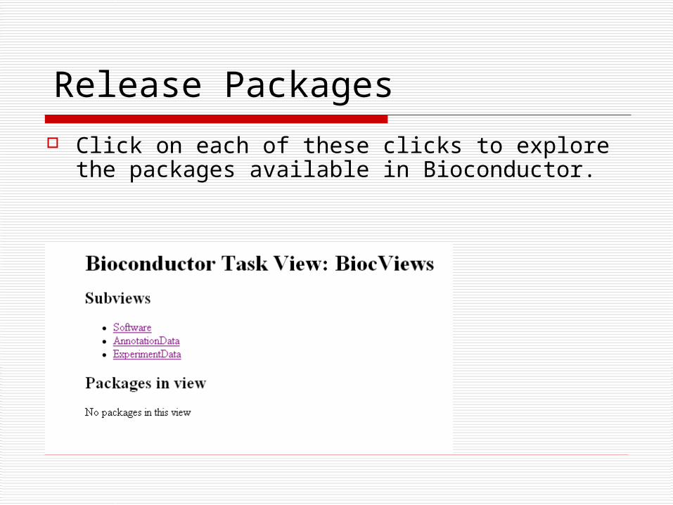
Release Packages

Click on each of these clicks to explore the packages available in Bioconductor.

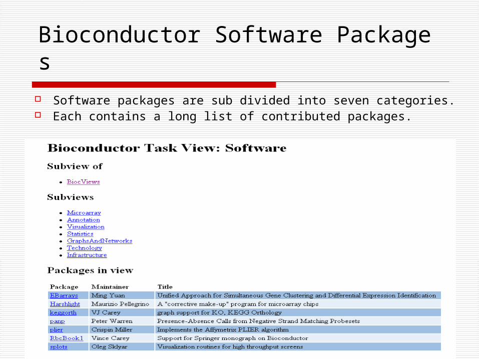
Bioconductor Software Packages Software packages are sub divided into seven categories. Each contains a long list of contributed packages.

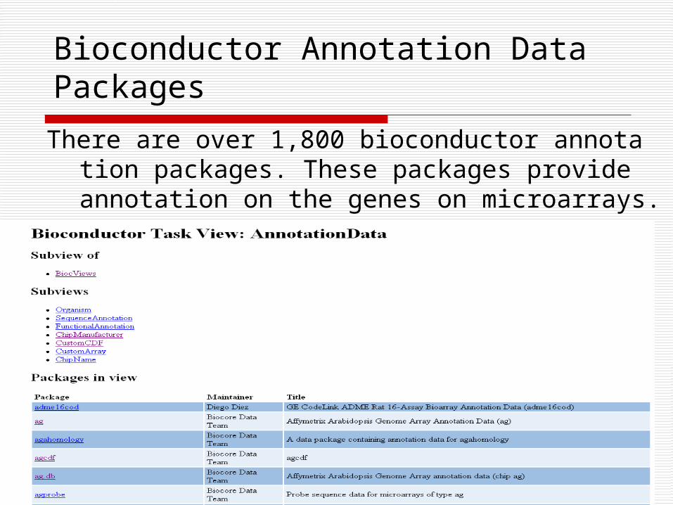
Bioconductor Annotation Data Packages

There are over 1,800 bioconductor annotation packages. These packages provide annotation on the genes on microarrays.

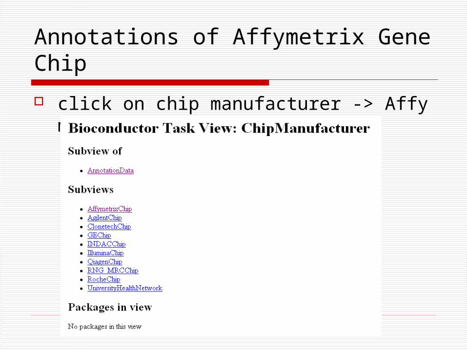
Annotations of Affymetrix GeneChip click on chip manufacturer -> Affymetrix

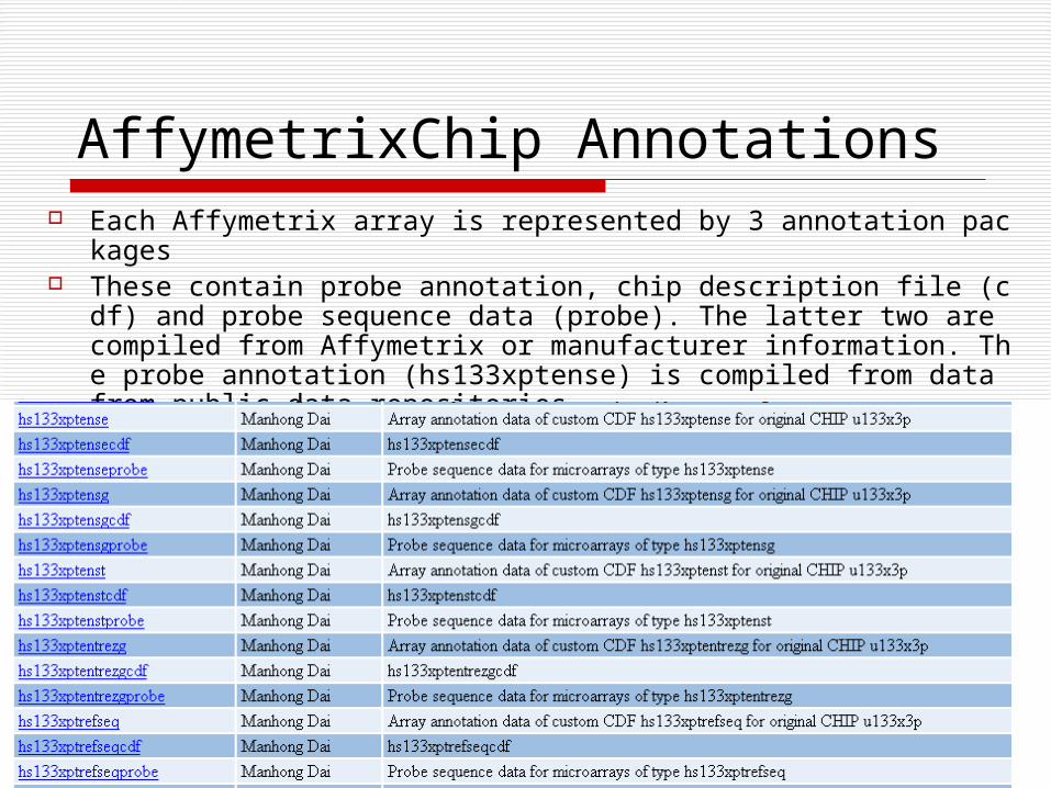
AffymetrixChip Annotations Each Affymetrix array is represented by 3 annotation packages These contain probe annotation, chip description file (cdf) and pr

obe sequence data (probe). The latter two are compiled from Affymetrix or manufacturer information. The probe annotation (hs133xptense) is compiled from data from public data repositories.

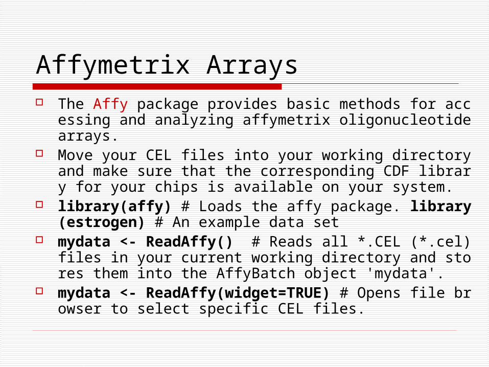
Affymetrix Arrays The Affy package provides basic methods for accessing and an

alyzing affymetrix oligonucleotide arrays. Move your CEL files into your working directory and make su

re that the corresponding CDF library for your chips is available on your system.

library(affy) # Loads the affy package. library(estrogen) # An example data set

mydata <- ReadAffy() # Reads all *.CEL (*.cel) files in your current working directory and stores them into the AffyBatch object 'mydata'.

mydata <- ReadAffy(widget=TRUE) # Opens file browser to select specific CEL files.

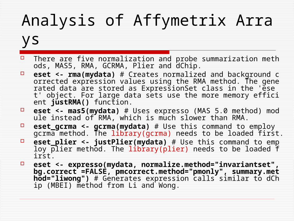
Analysis of Affymetrix Arrays There are five normalization and probe summarization methods, MAS5, R

MA, GCRMA, Plier and dChip. eset <- rma(mydata) # Creates normalized and background corrected exp

ression values using the RMA method. The generated data are stored as ExpressionSet class in the 'eset' object. For large data sets use the more memory efficient justRMA() function.

eset <- mas5(mydata) # Uses expresso (MAS 5.0 method) module instead of RMA, which is much slower than RMA.

eset_gcrma <- gcrma(mydata) # Use this command to employ gcrma method. The library(gcrma) needs to be loaded first.

eset_plier <- justPlier(mydata) # Use this command to employ plier method. The library(plier) needs to be loaded first.

eset <- expresso(mydata, normalize.method="invariantset", bg.correct =FALSE, pmcorrect.method="pmonly", summary.method="liwong") # Generates expression calls similar to dChip (MBEI) method from Li and Wong.

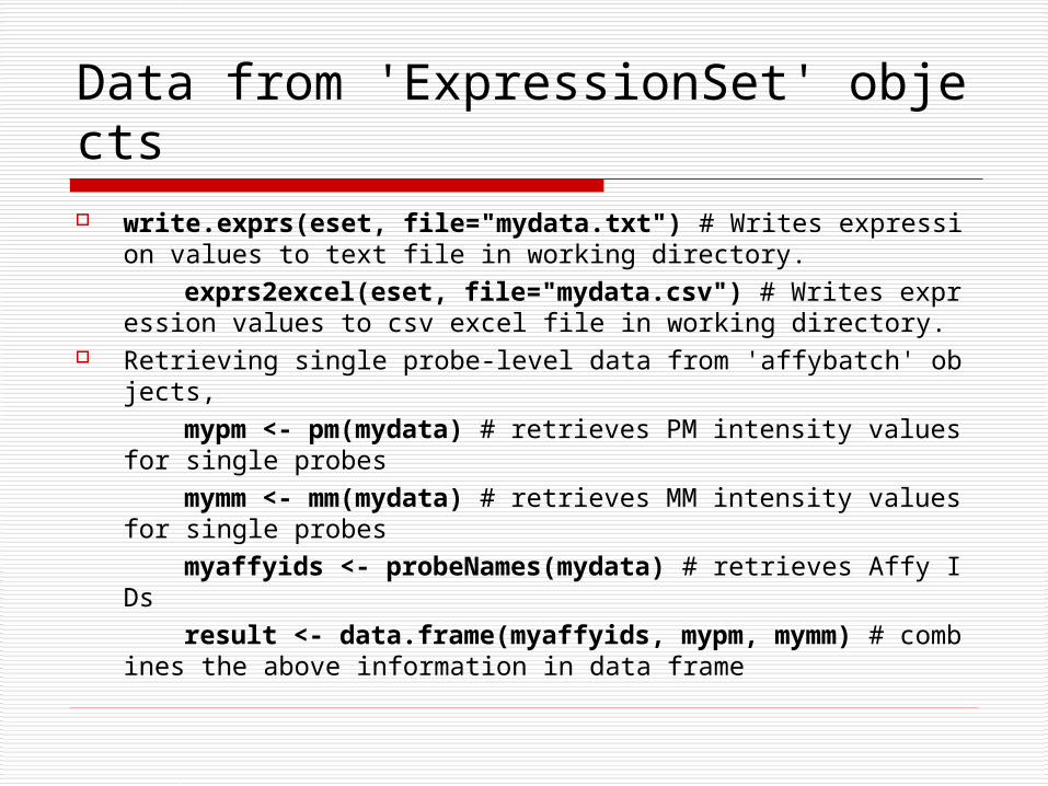
Data from 'ExpressionSet' objects write.exprs(eset, file="mydata.txt") # Writes expression values to tex

t file in working directory.

exprs2excel(eset, file="mydata.csv") # Writes expression values to csv excel file in working directory.

Retrieving single probe-level data from 'affybatch' objects,

mypm <- pm(mydata) # retrieves PM intensity values for single probes

mymm <- mm(mydata) # retrieves MM intensity values for single probes

myaffyids <- probeNames(mydata) # retrieves Affy IDs

result <- data.frame(myaffyids, mypm, mymm) # combines the above information in data frame

Working with 'ExpressionSet' objects eset; pData(eset) # Provides summary information of ExpressionSet o

bject 'eset' and lists the analyzed file names.

exprs(eset)[10:20,1:4]; exprs(eset)[c("1910_s_at","1933_g_at"),1:4] # Retrieves specific rows and fields of ExpressionSet object.

test <- as.data.frame(exprs(eset)); eset2 <-new("ExpressionSet", exprs = as.matrix(test), annotation="hgu95av2"); eset2 # Example for creating an ExpressionSet object from a data frame. To create the object from an external file, use the read.delim() function first and then convert it accordingly.

data.frame(eset) # Prints content of 'eset' as data frame to STDOUT.

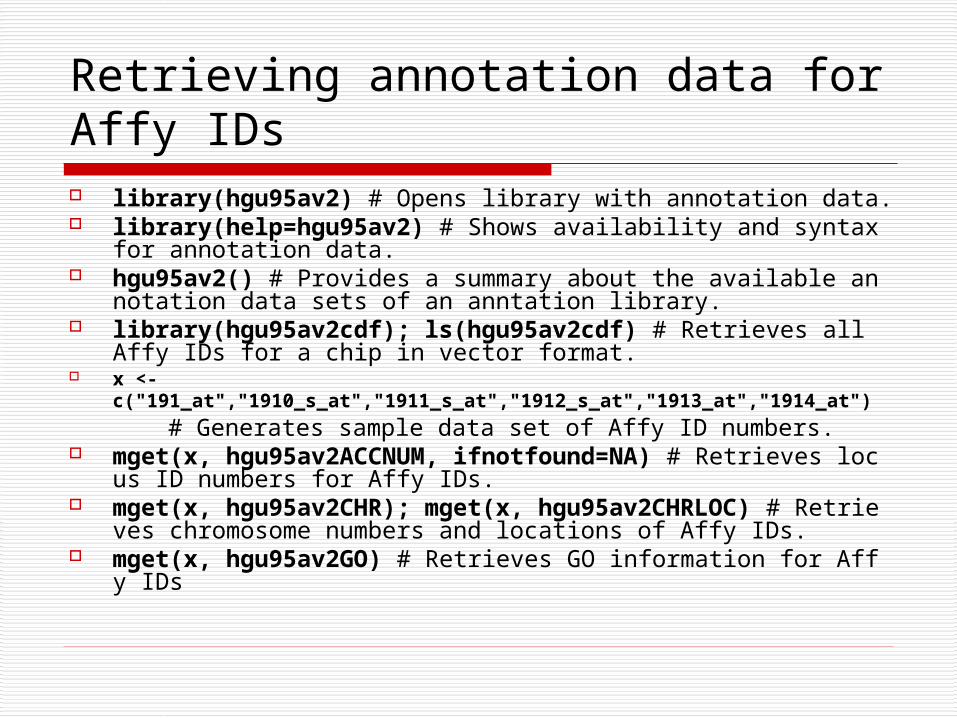
Retrieving annotation data for Affy IDs library(hgu95av2) # Opens library with annotation data. library(help=hgu95av2) # Shows availability and syntax for annotatio

n data. hgu95av2() # Provides a summary about the available annotation data s

ets of an anntation library. library(hgu95av2cdf); ls(hgu95av2cdf) # Retrieves all Affy IDs for a

chip in vector format. x <-c("191_at","1910_s_at","1911_s_at","1912_s_at","1913_at","1914_at") # Generates sample data set of Affy ID numbers. mget(x, hgu95av2ACCNUM, ifnotfound=NA) # Retrieves locus ID n

umbers for Affy IDs. mget(x, hgu95av2CHR); mget(x, hgu95av2CHRLOC) # Retrieves c

hromosome numbers and locations of Affy IDs. mget(x, hgu95av2GO) # Retrieves GO information for Affy IDs

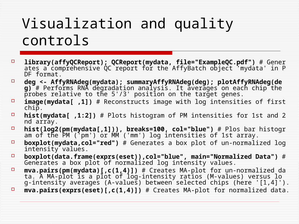
Visualization and quality controls library(affyQCReport); QCReport(mydata, file="ExampleQC.pdf") # Generates

a comprehensive QC report for the AffyBatch object 'mydata' in PDF format. deg <- AffyRNAdeg(mydata); summaryAffyRNAdeg(deg); plotAffyRNAdeg(deg)

# Performs RNA degradation analysis. It averages on each chip the probes relative to the 5'/3' position on the target genes.

image(mydata[ ,1]) # Reconstructs image with log intensities of first chip. hist(mydata[ ,1:2]) # Plots histogram of PM intensities for 1st and 2nd array. hist(log2(pm(mydata[,1])), breaks=100, col="blue") # Plos bar histogram of the PM

('pm') or MM ('mm') log intensities of 1st array. boxplot(mydata,col="red") # Generates a box plot of un-normalized log intensity val

ues. boxplot(data.frame(exprs(eset)),col="blue", main="Normalized Data") # Generat

es a box plot of normalized log intensity values. mva.pairs(pm(mydata)[,c(1,4)]) # Creates MA-plot for un-normalized data. A MA-pl

ot is a plot of log-intensity ratios (M-values) versus log-intensity averages (A-values) between selected chips (here '[1,4]').

mva.pairs(exprs(eset)[,c(1,4)]) # Creates MA-plot for normalized data.

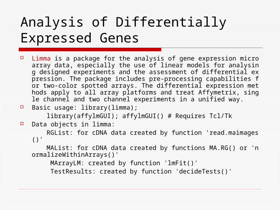
Analysis of Differentially Expressed Genes Limma is a package for the analysis of gene expression microarray data,

especially the use of linear models for analysing designed experiments and the assessment of differential expression. The package includes pre-processing capabilities for two-color spotted arrays. The differential expression methods apply to all array platforms and treat Affymetrix, single channel and two channel experiments in a unified way.

Basic usage: library(limma); library(affylmGUI); affylmGUI() # Requires Tcl/Tk Data objects in limma: RGList: for cDNA data created by function 'read.maimages()' MAList: for cDNA data created by functions MA.RG() or 'normalizeWi

thinArrays()' MArrayLM: created by function 'lmFit()' TestResults: created by function 'decideTests()'

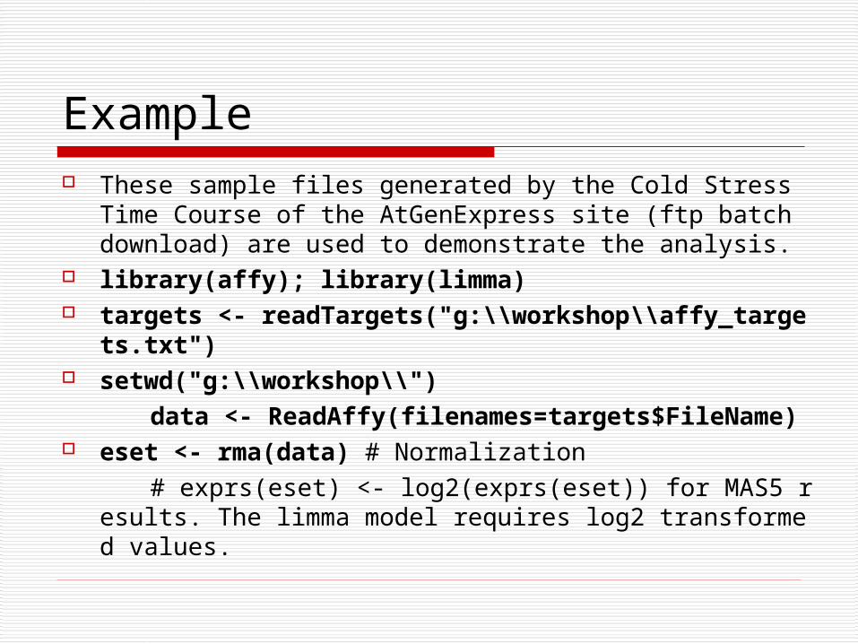
Example These sample files generated by the Cold Stress Time Course

of the AtGenExpress site (ftp batch download) are used to demonstrate the analysis.

library(affy); library(limma) targets <- readTargets("g:\\workshop\\affy_targets.txt") setwd("g:\\workshop\\")

data <- ReadAffy(filenames=targets$FileName) eset <- rma(data) # Normalization

# exprs(eset) <- log2(exprs(eset)) for MAS5 results. The limma model requires log2 transformed values.

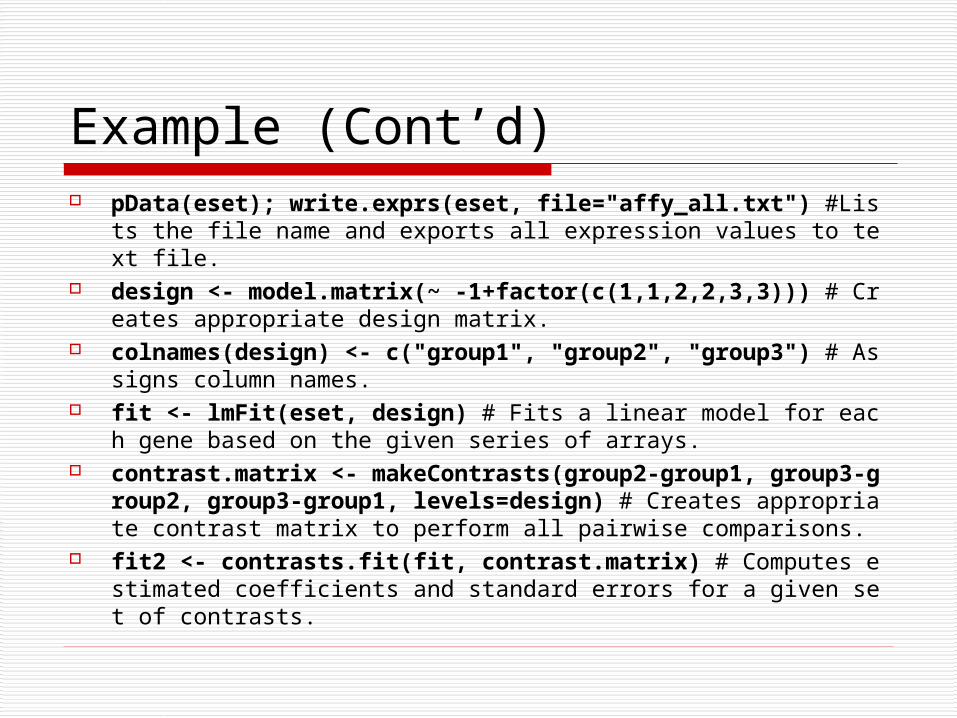
Example (Cont’d) pData(eset); write.exprs(eset, file="affy_all.txt") #Lists the file nam

e and exports all expression values to text file. design <- model.matrix(~ -1+factor(c(1,1,2,2,3,3))) # Creates appropr

iate design matrix. colnames(design) <- c("group1", "group2", "group3") # Assigns co

lumn names. fit <- lmFit(eset, design) # Fits a linear model for each gene based on t

he given series of arrays. contrast.matrix <- makeContrasts(group2-group1, group3-group2,

group3-group1, levels=design) # Creates appropriate contrast matrix to perform all pairwise comparisons.

fit2 <- contrasts.fit(fit, contrast.matrix) # Computes estimated coefficients and standard errors for a given set of contrasts.

Example (Cont’d) fit2 <- eBayes(fit2) # Computes moderated t-statistics and log-odds of

differential expression by empirical Bayes topTable(fit2, coef=1, adjust="fdr", sort.by="B", number=10) # G

enerates list of top 10 ('number=10') differentially expressed genes sorted by B-values ('sort.by=B') for first comparison group.

write.table(topTable(fit2, coef=1, adjust="fdr", sort.by="B", number=500), file="limma_complete.xls", row.names=F, sep="\t") # Exports complete limma statistics table for first comparison group.

results <- decideTests(fit2, p.value=0.05); vennDiagram(results) # Creates venn diagram of all D.E. genes at the level of 0.05. x <- topTable(fit2, coef=1, adjust="fdr", sort.by="P", number=50000);

y <- x[x$P.Value < 0.05,]; y <- x[x$P.Value < 0.01 & (x$logFC > 1 | x$logFC < -1) & x$AveExpr

> 10,] print("Number of genes in this list:"); length(y$ID)

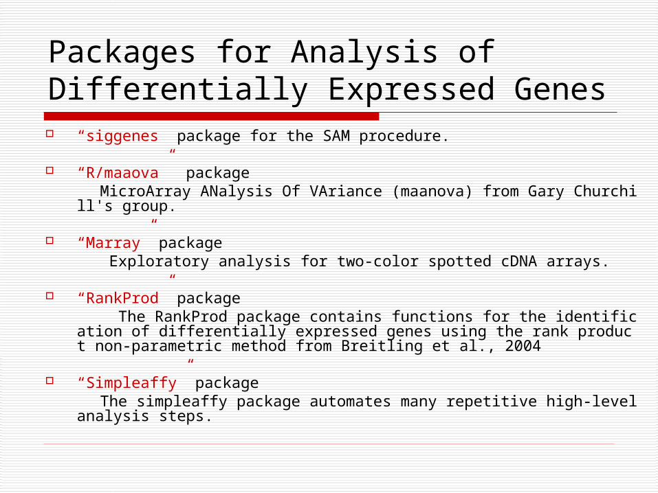
Packages for Analysis of Differentially Expressed Genes “siggenes” package for the SAM procedure.

“R/maaova” package MicroArray ANalysis Of VAriance (maanova) from Gary Churchill's group.

“Marray” package Exploratory analysis for two-color spotted cDNA arrays.

“RankProd” package The RankProd package contains functions for the identification of differentially exp

ressed genes using the rank product non-parametric method from Breitling et al., 2004

“Simpleaffy” package The simpleaffy package automates many repetitive high-level analysis steps.

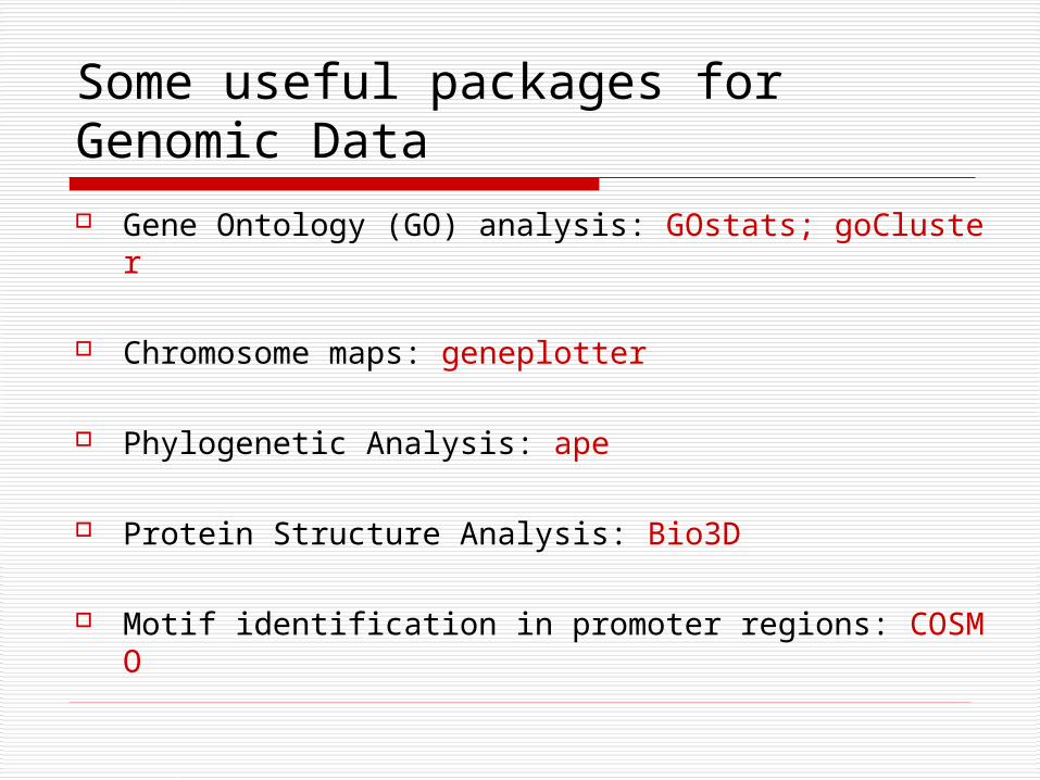
Some useful packages for Genomic Data

Gene Ontology (GO) analysis: GOstats; goCluster

Chromosome maps: geneplotter

Phylogenetic Analysis: ape

Protein Structure Analysis: Bio3D

Motif identification in promoter regions: COSMO

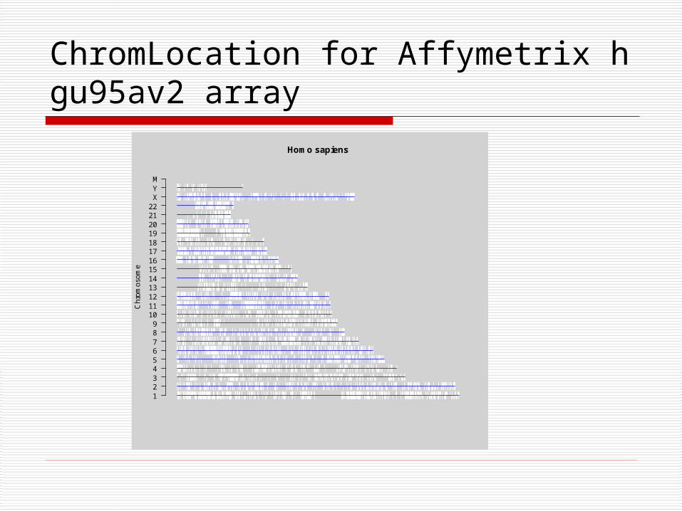
ChromLocation for Affymetrix hgu95av2 array

Homo sapiens

Ch

rom

oso

me

123456789

10111213141516171819202122XYM

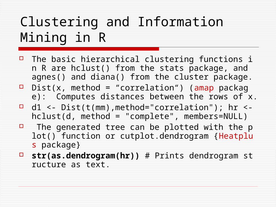
Clustering and Information Mining in R The basic hierarchical clustering functions in R are hclust()

from the stats package, and agnes() and diana() from the cluster package.

Dist(x, method = “correlation“) (amap package): Computes distances between the rows of x.

d1 <- Dist(t(mm),method="correlation"); hr <- hclust(d, method = "complete", members=NULL)

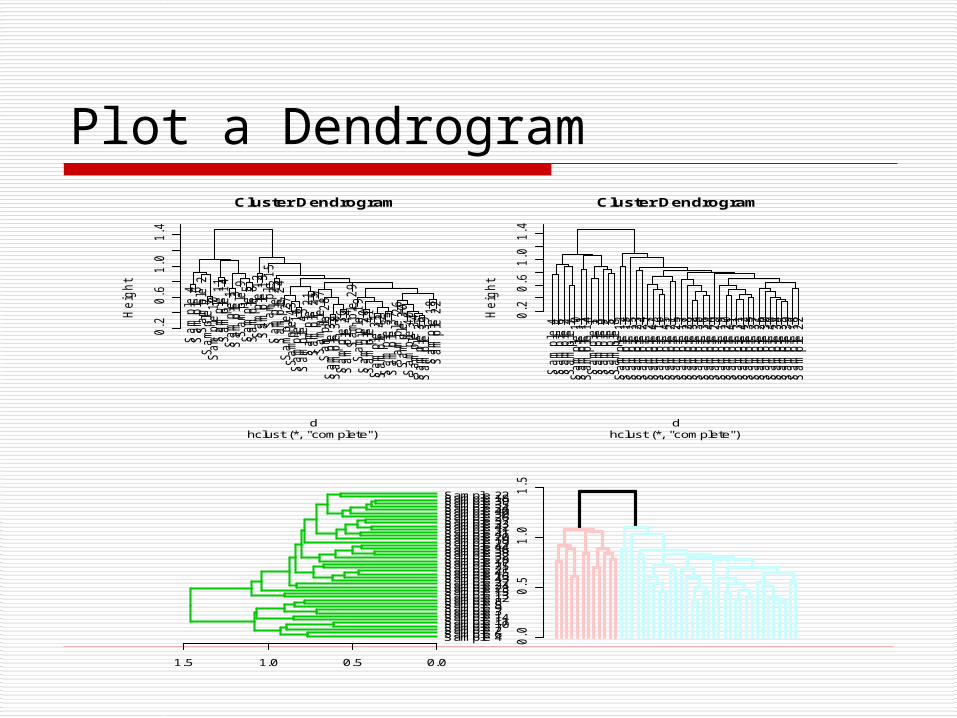
The generated tree can be plotted with the plot() function or cutplot.dendrogram {Heatplus package}

str(as.dendrogram(hr)) # Prints dendrogram structure as text.

Plot a Dendrogram S

am

ple

4S

am

ple

6S

am

ple

2S

am

ple

7S

am

ple

10

Sam

ple

11

Sam

ple

14

Sam

ple

1S

am

ple

3S

am

ple

9S

am

ple

5S

am

ple

8S

am

ple

12

Sam

ple

13

Sam

ple

15

Sam

ple

23

Sam

ple

24

Sam

ple

27

Sam

ple

43

Sam

ple

16

Sam

ple

45

Sam

ple

21

Sam

ple

25

Sam

ple

17

Sam

ple

28

Sam

ple

32

Sam

ple

38

Sam

ple

36

Sam

ple

44

Sam

ple

29

Sam

ple

19

Sam

ple

20

Sam

ple

41

Sam

ple

31

Sam

ple

42

Sam

ple

33

Sam

ple

37

Sam

ple

26

Sam

ple

30

Sam

ple

40

Sam

ple

34

Sam

ple

35

Sam

ple

39

Sam

ple

18

Sam

ple

22

0.2

0.6

1.0

1.4

Cluster Dendrogram

hclust (*, "complete")d

Heig

ht

Sam

ple

4S

am

ple

6S

am

ple

2S

am

ple

7S

am

ple

10

Sam

ple

11

Sam

ple

14

Sam

ple

1S

am

ple

3S

am

ple

9S

am

ple

5S

am

ple

8S

am

ple

12

Sam

ple

13

Sam

ple

15

Sam

ple

23

Sam

ple

24

Sam

ple

27

Sam

ple

43

Sam

ple

16

Sam

ple

45

Sam

ple

21

Sam

ple

25

Sam

ple

17

Sam

ple

28

Sam

ple

32

Sam

ple

38

Sam

ple

36

Sam

ple

44

Sam

ple

29

Sam

ple

19

Sam

ple

20

Sam

ple

41

Sam

ple

31

Sam

ple

42

Sam

ple

33

Sam

ple

37

Sam

ple

26

Sam

ple

30

Sam

ple

40

Sam

ple

34

Sam

ple

35

Sam

ple

39

Sam

ple

18

Sam

ple

220

.20.6

1.0

1.4

Cluster Dendrogram

hclust (*, "complete")d

Heig

ht

1.5 1.0 0.5 0.0

Sample 4Sample 6Sample 2Sample 7Sample 10Sample 11Sample 14Sample 1Sample 3Sample 9Sample 5Sample 8Sample 12Sample 13Sample 15Sample 23Sample 24Sample 27Sample 43Sample 16Sample 45Sample 21Sample 25Sample 17Sample 28Sample 32Sample 38Sample 36Sample 44Sample 29Sample 19Sample 20Sample 41Sample 31Sample 42Sample 33Sample 37Sample 26Sample 30Sample 40Sample 34Sample 35Sample 39Sample 18Sample 22

0.0

0.5

1.0

1.5

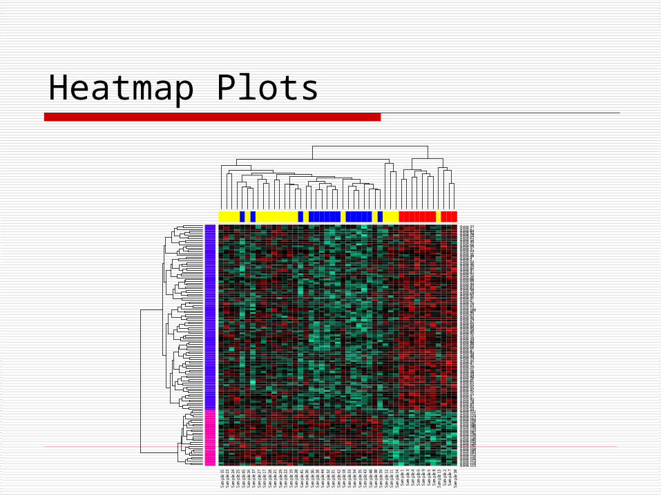
Heatmap Plots

Sam

ple

15S

ampl

e 23

Sam

ple

24S

ampl

e 25

Sam

ple

45S

ampl

e 16

Sam

ple

37S

ampl

e 27

Sam

ple

17S

ampl

e 28

Sam

ple

21S

ampl

e 29

Sam

ple

22S

ampl

e 19

Sam

ple

20S

ampl

e 41

Sam

ple

26S

ampl

e 36

Sam

ple

38S

ampl

e 44

Sam

ple

32S

ampl

e 31

Sam

ple

42S

ampl

e 18

Sam

ple

33S

ampl

e 34

Sam

ple

35S

ampl

e 43

Sam

ple

40S

ampl

e 30

Sam

ple

39S

ampl

e 12

Sam

ple

11S

ampl

e 14

Sam

ple

1S

ampl

e 3

Sam

ple

4S

ampl

e 6

Sam

ple

9S

ampl

e 5

Sam

ple

8S

ampl

e 13

Sam

ple

2S

ampl

e 7

Sam

ple

10

Gene 113Gene 116Gene 114Gene 119Gene 126Gene 124Gene 112Gene 103Gene 105Gene 110Gene 121Gene 102Gene 128Gene 125Gene 109Gene 120Gene 115Gene 130Gene 107Gene 127Gene 129Gene 106Gene 108Gene 101Gene 118Gene 104Gene 117Gene 123Gene 111Gene 122Gene 44Gene 58Gene 83Gene 97Gene 10Gene 79Gene 99Gene 5Gene 37Gene 21Gene 75Gene 27Gene 55Gene 57Gene 62Gene 61Gene 81Gene 18Gene 90Gene 34Gene 20Gene 28Gene 11Gene 29Gene 15Gene 9Gene 35Gene 32Gene 73Gene 98Gene 30Gene 89Gene 8Gene 51Gene 68Gene 69Gene 80Gene 88Gene 24Gene 39Gene 71Gene 72Gene 85Gene 50Gene 95Gene 48Gene 23Gene 65Gene 47Gene 74Gene 26Gene 63Gene 25Gene 86Gene 100Gene 17Gene 92Gene 14Gene 76Gene 6Gene 41Gene 45Gene 91Gene 64Gene 78Gene 54Gene 82Gene 42Gene 94Gene 52Gene 60Gene 66Gene 38Gene 77Gene 87Gene 3Gene 96Gene 43Gene 16Gene 36Gene 59Gene 2Gene 4Gene 40Gene 31Gene 12Gene 49Gene 7Gene 19Gene 56Gene 22Gene 46Gene 13Gene 67Gene 53Gene 70Gene 93Gene 84Gene 1Gene 33

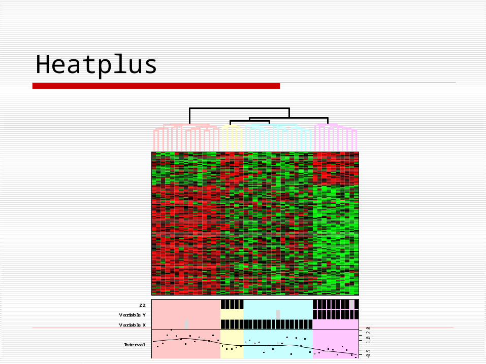
Heatplus

Variable X

Variable Y

ZZ

-0.5

1.0

2.0

Interval