Embed Size (px)
Citation preview
Modelling and Control of anInverted Pendulum Turbine
Sergi Rotger Griful
Kongens Lyngby 2012IMM-M.Sc.-2012-66

Technical University of DenmarkInformatics and Mathematical ModellingBuilding 321, DK-2800 Kongens Lyngby, DenmarkPhone +45 45253351, Fax +45 [email protected] IMM-M.Sc.-2012-66

Summary
The current energy situation is untenable in a long term. A change in the energysector is required and the wind energy is postulated as a good candidate for thisevolution.
There are many ways of improving the wind energy, either building bigger struc-tures able to generate large amounts of electricity either investigating new im-provements to make wind energy more profitable. In this project the feasibilityof a new kind of wind turbine is studied.
This thesis deals with the achievement of getting a proper mathematical modelof a new kind of wind turbine, called the inverted pendulum turbine, but alsodesigning a controller able to command this great structure.
The inverted pendulum turbine is inherently unstable system. In order to controlthis wind turbine an optimal control has been investigated: the linear quadraticregulator.
This project studies the feasibility of this uncommon wind turbine system designbut also promotes sustainable energy and opens a wide range of new possibleimplementations in the world of wind turbines.

ii

Resum
La situació energètica actual és insostenible a llarg termini. El sector energèticestà demanant a crits una reestructuració important i l’energia eòlica es postulacom possible motor d’aquest canvi.
Hi ha moltes maneres de millorar l’energia eòlica, ja sigui construint aerogener-adors de dimensions més grans capaços de produir més electricitat o investigantnoves millores per tal de fer l’energia eòlica més rentable. En aquest projectes’estudia la viabilitat d’un nou model de turbina vent.
Aquest treball té el repte d’aconseguir un model matemàtic fiable d’aquesta novaturbina de vent, anomenada turbina de pèndul invertit, i dissenyar un reguladorcapaç de controlar aquesta gran infraestructura.
La turbina de pèndul invertit és, per la seva naturalesa, un sistema inestable.Per tal de poder controlar-la s’ha utilitzat una tècnica de regulació òptima comara és el control lineal quadràtic.
Aquest projecte estudia la viabilitat d’aquest estrambòtic aerogenerador aixícom també promou les energies renovables obrint un ampli ventall de futuresaplicacions en el món de l’energia eòlica.

iv
Preface
The project was carried out at the department of Informatics and MathematicalModelling at the Technical University of Denmark with the cooperation of theDanish wind company Vestas Wind Systems A/S in fulfilment of the require-ments for acquiring an M.Sc. degree in Industrial Engineering in Automationand Control.
This project was proposed by the engineer Keld Hammerum from Vestas WindSystems A/S and have been supervised by the control engineer Fabio Caponettifrom Vestas Turbines R&D, by the PhD student Mahmood Mirzaei from DTUInformatics, by the Associate Professor Hans Henrik Niemann from DTU Elec-trical Engineering and by the Associate Professor Niels Kjølstad Poulsen fromDTU Informatics.
The thesis deals with the achievement of modelling and controlling a new kindof wind turbine known as the inverted pendulum turbine. The inverted pen-dulum turbine is a Horizontal Axes Wind Turbine with and additional degreeof freedom: the inclination of the tower. The controller then has the goal ofmaximizing the produced electrical power while avoiding the turbine to collapse.
Lyngby, 16-July-2012
Sergi Rotger Griful

vi

Acknowledgements
As an Erasmus student I had to choose a project to work on before arriving toDenmark. After searching and considering many different options I contactedwith the Associate Professor Niels Kjølastad Poulsen who offered me a veryinteresting and challenging project. For giving me the chance to work with himand for all his support and guidance during the realization of this thesis I wouldlike to express my most sincere gratitude to him.
I would also like to thank the Associate Professor Hans Henrik Niemann for hisadvices and inspiration, and the PhD student Mahmood Mirzaei for all the timethat has dedicated to me which has been very useful and instructive.
I would like to express my gratitude to the control engineer Fabio Caponettibecause besides the distance he has always been there ready to help and giveme useful advices. I would also like to thank the M.Sc. student Martin Klaucofor many fruitful and inspiring discussions.
And last but not least I would like to express my gratitude to my family andfriends, specially my mother Eulàlia, my father Jordi, my sister Carla and mygirlfriend Núria, because besides the large distance between us I have never feltalone and I have always received support from them.

viii

Nomenclature
v m/s Wind speedv m/s2 Wind accelerationvm m/s Mean component of the wind speed modelvt m/s Turbulent component of the wind speed modelPw W Power available in the windPr W Power extracted by the rotorPe W Electrical powerη − Efficiency of mechanical-electrical conversionρa kg/m3 Air densityg m/s2 Gravity constant

x
At m2 Swept area by the wind turbine bladesR m Rotor radiusCp − Power coefficientCt − Thrust coefficientλ − Tip speed ratioωr rad/s Rotor angular speedωg rad/s Generator angular speedβ deg Pitch angleTr N m Aerodynamic torqueTg N m Generator torqueFt N Thrust forceN − Gearbox ratioKt N/m Tower spring constantDt N/m s Tower damping constantMt kg Mass of the tower, rotor, nacelle and hubKat N/rad Tower angular spring constant
Dat Ns/rad Tower angular damping constant
Mat Ns2/rad Angular equivalence to Mt
fn Hz Natural frequency of the tower Fore-AftJg kg m2 Inertia of the generatorJr kg m2 Inertia of the rotorJ kg m2 Inertia of the generator and rotor
θ rad Angle of inclination of the towerθ rad/s Speed of inclination of the towerθ rad/s2 Acceleration of inclination of the tower
nx − Number of statesny − Number of outputsnu − Number of inputsnd − Number of disturbances
xi
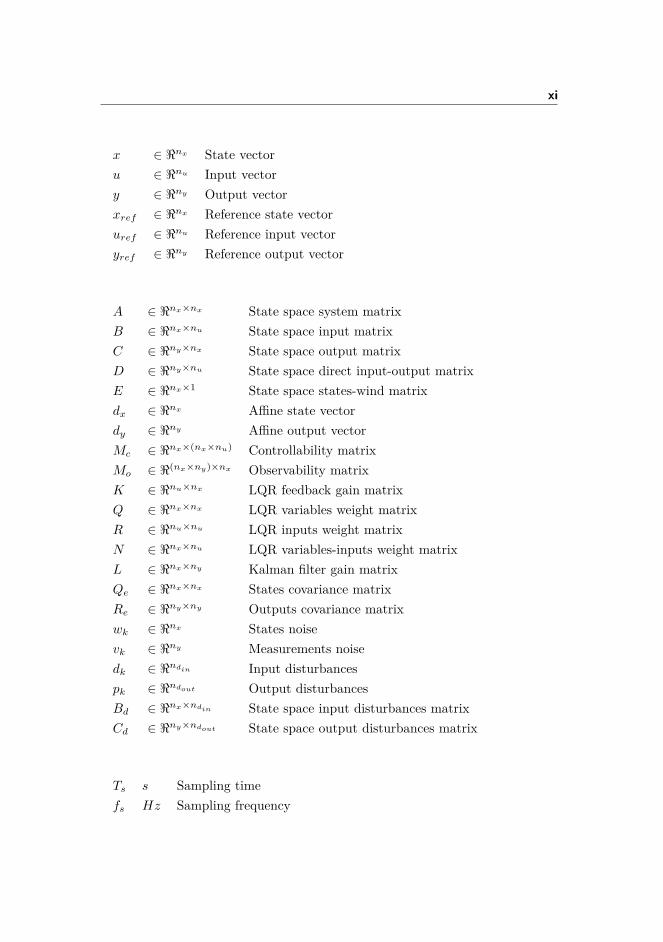
x ∈ <nx State vectoru ∈ <nu Input vectory ∈ <ny Output vectorxref ∈ <nx Reference state vectoruref ∈ <nu Reference input vectoryref ∈ <ny Reference output vector
A ∈ <nx×nx State space system matrixB ∈ <nx×nu State space input matrixC ∈ <ny×nx State space output matrixD ∈ <ny×nu State space direct input-output matrixE ∈ <nx×1 State space states-wind matrixdx ∈ <nx Affine state vectordy ∈ <ny Affine output vectorMc ∈ <nx×(nx×nu) Controllability matrixMo ∈ <(nx×ny)×nx Observability matrixK ∈ <nu×nx LQR feedback gain matrixQ ∈ <nx×nx LQR variables weight matrixR ∈ <nu×nu LQR inputs weight matrixN ∈ <nx×nu LQR variables-inputs weight matrixL ∈ <nx×ny Kalman filter gain matrixQe ∈ <nx×nx States covariance matrixRe ∈ <ny×ny Outputs covariance matrixwk ∈ <nx States noisevk ∈ <ny Measurements noisedk ∈ <ndin Input disturbancespk ∈ <ndout Output disturbancesBd ∈ <nx×ndin State space input disturbances matrixCd ∈ <ny×ndout State space output disturbances matrix
Ts s Sampling timefs Hz Sampling frequency

xii

Contents
Summary i
Resum iii
Preface v
Acknowledgements vii
Nomenclature ix
1 Introduction 11.1 The Inverted Pendulum Turbine . . . . . . . . . . . . . . . . . . 21.2 Control . . . . . . . . . . . . . . . . . . . . . . . . . . . . . . . . 51.3 Objectives . . . . . . . . . . . . . . . . . . . . . . . . . . . . . . . 61.4 Thesis Overview . . . . . . . . . . . . . . . . . . . . . . . . . . . 6
2 Modelling and Analysis 92.1 Wind Turbines and Wind Energy Basics . . . . . . . . . . . . . . 9
2.1.1 Wind Energy Conversion Systems . . . . . . . . . . . . . 92.1.2 Basic Concepts of the Wind Energy Conversion . . . . . 11
2.2 Non-Linear Model . . . . . . . . . . . . . . . . . . . . . . . . . . 162.2.1 Rotor . . . . . . . . . . . . . . . . . . . . . . . . . . . . . 162.2.2 Hinge Tower . . . . . . . . . . . . . . . . . . . . . . . . . 17
2.3 Operation Modes and Steady State Analysis . . . . . . . . . . . 212.3.1 Operation Regions Definition . . . . . . . . . . . . . . . . 212.3.2 Steady State Analysis of the Reference Wind Turbine . . 23
2.4 Linear Model . . . . . . . . . . . . . . . . . . . . . . . . . . . . . 292.4.1 Wind Turbine Model . . . . . . . . . . . . . . . . . . . . . 292.4.2 The Wind Model . . . . . . . . . . . . . . . . . . . . . . . 32

xiv CONTENTS
2.4.3 Affine Model . . . . . . . . . . . . . . . . . . . . . . . . . 342.5 Model Analysis . . . . . . . . . . . . . . . . . . . . . . . . . . . . 36
2.5.1 Characteristics of the System . . . . . . . . . . . . . . . . 362.5.2 Model Verification . . . . . . . . . . . . . . . . . . . . . . 39
3 Control Methods 433.1 Kalman Filter . . . . . . . . . . . . . . . . . . . . . . . . . . . . 433.2 Linear Quadratic Regulator . . . . . . . . . . . . . . . . . . . . . 463.3 Linear Quadratic Gaussian Control . . . . . . . . . . . . . . . . 493.4 Offset-Free Methods . . . . . . . . . . . . . . . . . . . . . . . . . 51
3.4.1 Integral Action . . . . . . . . . . . . . . . . . . . . . . . . 513.4.2 Disturbance Modelling . . . . . . . . . . . . . . . . . . . . 52
4 Implementation and Results 554.1 Baseline Controller . . . . . . . . . . . . . . . . . . . . . . . . . 554.2 Control Strategy . . . . . . . . . . . . . . . . . . . . . . . . . . . 57
4.2.1 Control Objectives per Region . . . . . . . . . . . . . . . 574.2.2 Switching Criteria . . . . . . . . . . . . . . . . . . . . . . 594.2.3 Control Strategy Summary . . . . . . . . . . . . . . . . . 60
4.3 Control Implementation . . . . . . . . . . . . . . . . . . . . . . . 624.3.1 Discrete Model . . . . . . . . . . . . . . . . . . . . . . . . 624.3.2 Wind and States Estimation . . . . . . . . . . . . . . . . 624.3.3 Offset-Free Performance . . . . . . . . . . . . . . . . . . . 694.3.4 LQG . . . . . . . . . . . . . . . . . . . . . . . . . . . . . . 74
4.4 Comparison . . . . . . . . . . . . . . . . . . . . . . . . . . . . . . 824.4.1 Baseline Vs. LQG Controller . . . . . . . . . . . . . . . . 824.4.2 Stiff Vs. Hinge Tower . . . . . . . . . . . . . . . . . . . . 85
5 Conclusions and Perspectives 895.1 Conclusions . . . . . . . . . . . . . . . . . . . . . . . . . . . . . . 895.2 Perspectives . . . . . . . . . . . . . . . . . . . . . . . . . . . . . . 92
A Tower Spring-Mass-Damper Justification 93
B System Parameters 95
Bibliography 97

Chapter 1
Introduction
According to the International Energy Agency (IEA) more than 50% of thefinal energy consumed in 2009 came from burning oil and gas. This kind ofenergy sources are contributing with their high CO2 emissions to the globalwarming. The energy sources used nowadays and the fact that every day theenergy consumption is growing are bringing the world to a dead-end.
To try to redirect the current situation there are two possible solutions: changingthe habits of people by trying to reduce the energy consumption and changingthe current energy sources by ones with less environment impact like renewableenergies.
Changing the habits of people is always a really challenging task and do notseems possible to see results in a short term.
Promoting renewable energies in front of the polluting ones is not easy as wellbut the energy sector is claiming for a big change.
There are many renewable energies and most of them are growing since theenergy change is becoming a necessity. Because of its good results, the windenergy is gaining importance in the energy sector and has experienced a dramaticgrowth since the turn of the 21st century. According to the IEA the globalinstalled capacity at the end of 2011 was around 238 GW, up from 18 GW at

2 Introduction
the end of 2000.
Besides the important environmental impact that the wind turbines have tothe nature and wildlife they do not have any other big drawbacks. This en-vironmental impact is normally evaluated during the sitting process of windfarms avoiding some places like natural reserves or the main routes of migrationbirds. Wind turbines are able to generate big amounts of ’clean energy’, theycan readjust the difference between the electrical offer and demand faster thanother energy sources... All these facts are making the wind energy a possible wayout to the difficult current situation. Companies and governments are aware ofthis situation and are investing in research and development of wind turbines.A good example of this situation is that, according to the IEA, ten Europeancountries have agreed to develop an offshore electricity grid in the North Sea toenable offshore wind developments.
Everyday wind energy companies are fabricating bigger turbines that are able toproduce more electrical power. For example the Danish wind turbine developerEdmond Muller has designed a 30 MW wind turbine which is higher than theEiffel Tower, but no wind company believe in his project. This shows thatthe size of wind turbine cannot be increased indefinitely, there is definitely anupper limit, there is going to be a moment that increasing the size will not beprofitable any more. That is the reason why new technical solutions, such theone developed in this project, are being investigated.
1.1 The Inverted Pendulum Turbine
Current wind turbines are huge structures with an important initial investment.In (Fingersh et al., 2006) there is a large description of the costs of the compo-nents of wind turbines and the start-up/installation costs for land based turbinesand off-shore turbines. To give an order of magnitude of the costs of a windturbine in tables 1.1 and 1.2 there is, respectively, a summary of the expensesin the land-based and in the off-shore case.
As it can be seen from the tables 1.1 and 1.2 , the cost of the tower accountsaround 10% of the total cost (material and installation) and around 15% of theturbine cost. The large cost of the tower stems from the fact that it needs tobe very stiff in order to withstand the bending moments of the thrust force ofthe wind. One possible solution to reduce the cost of the tower is the invertedpendulum turbine. In figure 1.1 a schematic of this wind turbine is presented.
The inverted pendulum turbine is a new kind of wind turbine which peculiarity

1.1 The Inverted Pendulum Turbine 3
Table 1.1: Land-Based 1.5-MW Baseline Turbine Costs in 2002.(Fingershet al., 2006)
Component Cost [$1.000] [%]Turbine cost 1.036 73.8Rotor 237 16.9Drive train, nacelle 617 44.0Control & Safety 35 2.5Tower 147 10.4Station cost 367 26.2Initial capital cost 1.403 100
Table 1.2: Offshore 3-MW Baseline Turbine Costs in 2005.(Fingersh et al.,2006)
Component Cost [$1.000] [%]Turbine cost 2.698 42.2Rotor 477 7.5Drive train, nacelle 1.425 22.3Control & Safety 60 0.9Tower 415 6.5Marinization 321 5.0Station cost 3.331 52.2Off-shore warranty premium 357 5.6Initial capital cost 6.386 100
4 Introduction
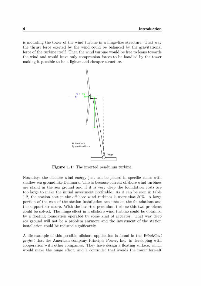
is mounting the tower of the wind turbine in a hinge-like structure. That waythe thrust force exerted by the wind could be balanced by the gravitationalforce of the turbine itself. Then the wind turbine would be free to leans towardsthe wind and would leave only compression forces to be handled by the towermaking it possible to be a lighter and cheaper structure.
Ft Fg
Hinge
=
Ft: thrust forceFg: gravitional force
Figure 1.1: The inverted pendulum turbine.
Nowadays the offshore wind energy just can be placed in specific zones withshallow sea ground like Denmark. This is because current offshore wind turbinesare stand in the sea ground and if it is very deep the foundation costs aretoo large to make the initial investment profitable. As it can be seen in table1.2, the station cost in the offshore wind turbines is more that 50%. A largeportion of the cost of the station installation accounts on the foundations andthe support structure. With the inverted pendulum turbine this two problemscould be solved. The hinge effect in a offshore wind turbine could be obtainedby a floating foundation operated by some kind of actuator. That way deepsea ground will not be a problem anymore and the investment of the stationinstallation could be reduced significantly.
A life example of this possible offshore application is found in the WindFloatproject that the American company Principle Power, Inc. is developing withcooperation with other companies. They have design a floating surface, whichwould make the hinge effect, and a controller that avoids the tower fore-aft

1.2 Control 5
motion caused by the wind gust an the sea motion. Right now they are stilldoing test in the coast of Portugal.
1.2 Control
These days wind turbines are controlled by a set of PI(D) controller such theone designed by the National Renewable Energies Laboratory in (Jonkman et al.,2009). The performance of this controllers is manually optimized and the tuningprocess is done by an engineer in an iterative process until the required perfor-mance is obtained. Then having good results depend on the experience of theengineer.
A possible alternative to this kind of controllers are the optimal controllers likeModel Predictive Controllers (MPC) and Linear Quadratic Regulators (LQR).This kind of regulators ensure an optimal performance having a good model ofthe wind turbine. Then the quality of the control action relies on the quality ofthe model. This is one of the reasons why companies are still working with setof PI(D) instead of optimal controllers.
Today there many techniques of system identification that can get a good modelsand some control method that are able to minimize the mismatch between amodel and its plant. In other sectors like the chemical world MPC has beenimplemented successfully and its to be expected that in the near future, thePI(D) controllers of the wind turbines would probably be replaced by moreefficient controllers such as MPC or LQR. Today there are many studies of thiskind of controllers over wind turbines, for example in (Henriksen, 2007) and(Gosk, 2011) the viability of the MPC to control wind turbines is studied and in(Mirzaei et al., 2012b) there is a very interesting approach of the robust MPCof a wind turbine over the full load region.
The Linear Quadratic Regulators are a proven control technique, that com-pared to the PI(D) ensures optimal performance, but do not need such a largecomputational models like the MPC. Compared to PI(D) controllers LinearQuadratic Regulators can work over multi-input multi-output (MIMO) systemswhile PI(D) need to work on single-input single-output(SISO) systems or over aMIMO systems separate in different SISO systems, but that is not always pos-sible. It is important to highlight that wind turbines are MIMO systems and inthis project the inverted pendulum turbine has been treated as that. Becauseof all this reasons the Linear Quadratic Regulator technique has been chosen tocontrol the inverted pendulum turbine.
6 Introduction
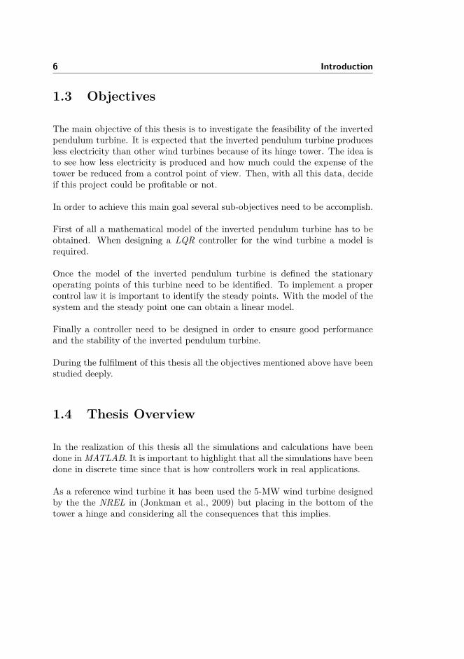
1.3 Objectives
The main objective of this thesis is to investigate the feasibility of the invertedpendulum turbine. It is expected that the inverted pendulum turbine producesless electricity than other wind turbines because of its hinge tower. The idea isto see how less electricity is produced and how much could the expense of thetower be reduced from a control point of view. Then, with all this data, decideif this project could be profitable or not.
In order to achieve this main goal several sub-objectives need to be accomplish.
First of all a mathematical model of the inverted pendulum turbine has to beobtained. When designing a LQR controller for the wind turbine a model isrequired.
Once the model of the inverted pendulum turbine is defined the stationaryoperating points of this turbine need to be identified. To implement a propercontrol law it is important to identify the steady points. With the model of thesystem and the steady point one can obtain a linear model.
Finally a controller need to be designed in order to ensure good performanceand the stability of the inverted pendulum turbine.
During the fulfilment of this thesis all the objectives mentioned above have beenstudied deeply.
1.4 Thesis Overview
In the realization of this thesis all the simulations and calculations have beendone inMATLAB. It is important to highlight that all the simulations have beendone in discrete time since that is how controllers work in real applications.
As a reference wind turbine it has been used the 5-MW wind turbine designedby the the NREL in (Jonkman et al., 2009) but placing in the bottom of thetower a hinge and considering all the consequences that this implies.

1.4 Thesis Overview 7
The report of this thesis is organized in four different parts according to chapters:
• Modelling and Analysis: In this part a basic introduction to windenergy is done. It is also shown how the model of the inverted pendulumhas been obtained. Then an analysis of the control properties of thisuncommon wind turbine has been done.
• Control Methods: In this part all the theoretical control methods usedare introduced.
• Implementation and Results: In this part all the methods men-tioned in the previous chapter have been put into practice. All the resultsobtained from the simulations are also shown in this part.
• Conclusions and Perspectives: In this final part the conclusions ofthe project are exposed and the possible future perspective of the thesisare presented.
It is assumed that the reader of this thesis have basic knowledge of physics andcontrol theory. However there is a brief mention of all the important conceptsused and a basic introduction to the world of wind energy and wind turbines.

8 Introduction
Chapter 2
Modelling and Analysis
In this chapter the reader can find a basic description of wind turbines andwind energy. Then the non-linear model of the inverted pendulum turbine ispresented. With the aim of maximizing the produced electrical power and sat-isfying some restrictions imposed by the wind turbine components the differentoperation modes of this peculiar wind turbine are defined and the steady stateanalysis for the baseline wind turbine is done. Finally the linear model is ob-tained and the basic properties of the system are analysed.
2.1 Wind Turbines and Wind Energy Basics
2.1.1 Wind Energy Conversion Systems
As mentioned in (Sathyajith, 2006) there are many different kind of Wind En-ergy Conversion Systems (WECS). The most commune WECS nowadays arethe Horizontal Axis Wind Turbines (HAWT) but it has not always been like this.By the end of the last century there was an intense research on the Vertical AxisWind Turbines (VAWT) but theses could not be as a reliable alternative as theHAWT. In this section a short introduction to the HAWT and the differentcomponents of this wind turbines is done.

10 Modelling and Analysis
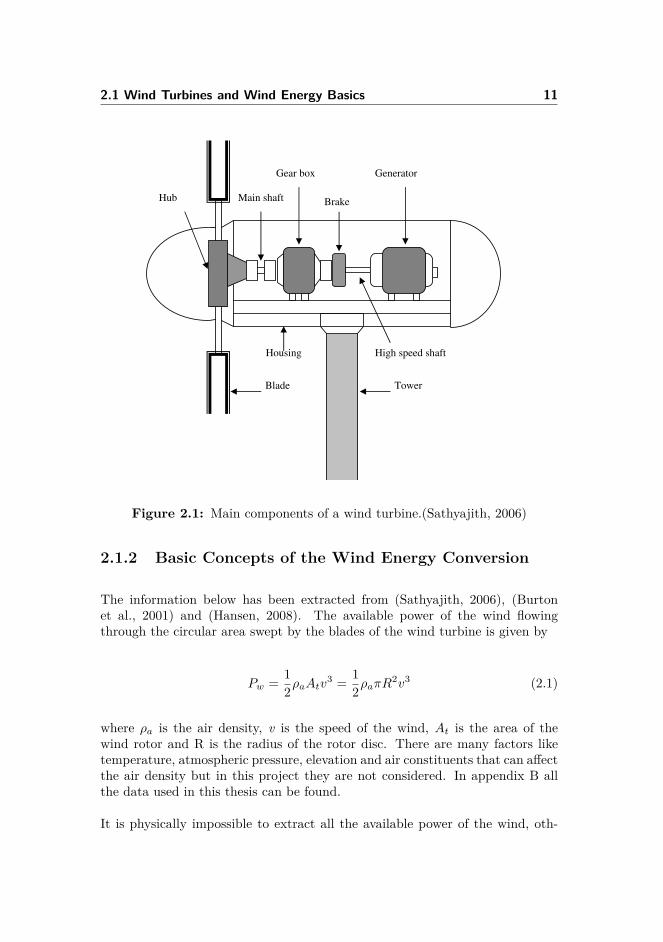
The HAWT is the wind turbine that one can see today on places where windenergy is present. They normally have three blades and their tower high canbe from some meters up to 100 m. The HAWT are big structures composedby many different components, the most important ones are listed below. Fora better understanding in figure 2.1 the disposition of all the mentioned com-ponents can be seen. All the information has been extracted from (Sathyajith,2006) and (Friis et al., 2010).
• Tower is the part that hold the nacelle (or housing) and the rotor inthe desired height. The towers of the HAWT are very stiff in order towithstand the bending moments from the thrust acting, exerted by thewind, on the turbine rotor.
• Rotor is the part that receives the energy from the wind and transformsit into mechanical power. The rotor is composed by the blades, the hub,the shaft and other components.
• Blades is the part responsible of transforming the kinetic energy fromthe wind into rotational motion. It is important to know that the blades,in order to control the energy extracted from the wind, are able to pitch.Pitching is the action of the blades of rotating along its axes.
• Hub is the part which connects all the blades and contain different com-ponents like the pitch system.
• Main shaft or low speed shaft is connected with the hub and is re-sponsible of transferring the rotational power into the gear box.
• Gear box is the responsible of transforming the low speed rotation comingfrom the low speed shaft into a more fast rotation which is suitable forthe electrical generator.
• Brake is the part responsible of stopping the wind turbine, for its safety,when the wind is too fast.
• High speed shaft is the part connected between the gear box and thegenerator.
• Generator is the part responsible of the transformation from mechanicalpower to electrical power.
• Nacelle or housing is the part that contains the shafts, gear box, brakeand the generator, besides other components.
2.1 Wind Turbines and Wind Energy Basics 1190 4 Wind energy conversion systems
Housing High speed shaft
Generator
Brake
Gear box
Main shaft Hub
Blade Tower
4.1 Wind electric generators
Fig. 4.1. Components of a wind electric generator
Electricity generation is the most important application of wind energy today. The major components of a commercial wind turbine are: 1. Tower2. Rotor 3. High speed and low speed shafts 4. Gear box 5. Generator 6. Sensors and yaw drive 7. Power regulation and controlling units 8. Safety systems The major components of the turbine are shown in Fig. 4.1.
Figure 2.1: Main components of a wind turbine.(Sathyajith, 2006)
2.1.2 Basic Concepts of the Wind Energy Conversion
The information below has been extracted from (Sathyajith, 2006), (Burtonet al., 2001) and (Hansen, 2008). The available power of the wind flowingthrough the circular area swept by the blades of the wind turbine is given by
Pw = 12ρaAtv
3 = 12ρaπR
2v3 (2.1)
where ρa is the air density, v is the speed of the wind, At is the area of thewind rotor and R is the radius of the rotor disc. There are many factors liketemperature, atmospheric pressure, elevation and air constituents that can affectthe air density but in this project they are not considered. In appendix B allthe data used in this thesis can be found.
It is physically impossible to extract all the available power of the wind, oth-

12 Modelling and Analysis
erwise the wind speed at the rotor front would be zero and the rotation of therotor would stop. It becomes necessary to introduce the concept of the powercoefficient Cp
Pr = PwCp (2.2)
Cp is the ratio between the power extracted by the rotor, Pr, and the poweravailable from the wind, Pw, and it has a theoretical upper limit of 16
27 knownas Betz limit. Modern wind turbines have a maximum power coefficient around0.5. The Cp coefficient is function of the pitch angle of the blades β and of thetip speed ratio λ, which is the ratio between the linear velocity of the tip of theblades and the wind speed
λ = ωrR
v(2.3)
The pitch angle is the rotational angle of the blades along their axes. When β iszero the blades are completely perpendicular to the wind. The figure 2.2 helpsto understand better the concept of the pitch angle β.
R
φr
θ�
wr
R
Figure 2.2: Detail of the pitch angle β and the rotational speed wr.(Henriksen,2007)
2.1 Wind Turbines and Wind Energy Basics 13
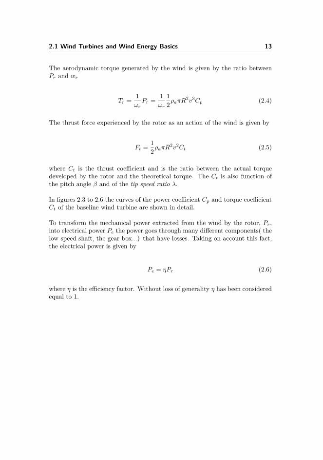
The aerodynamic torque generated by the wind is given by the ratio betweenPr and wr
Tr = 1ωrPr = 1
ωr
12ρaπR
2v3Cp (2.4)
The thrust force experienced by the rotor as an action of the wind is given by
Ft = 12ρaπR
2v2Ct (2.5)
where Ct is the thrust coefficient and is the ratio between the actual torquedeveloped by the rotor and the theoretical torque. The Ct is also function ofthe pitch angle β and of the tip speed ratio λ.
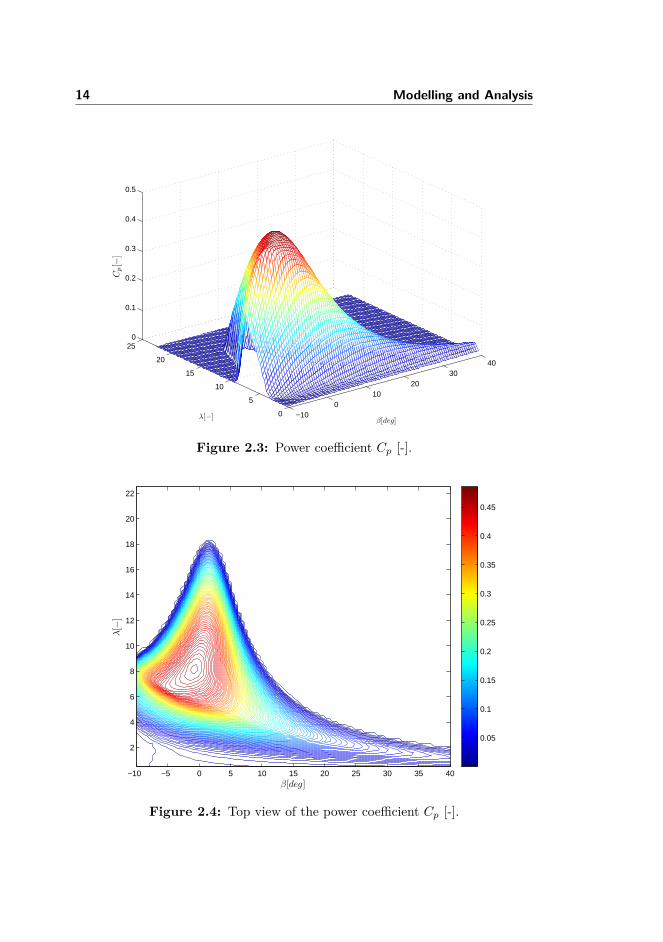
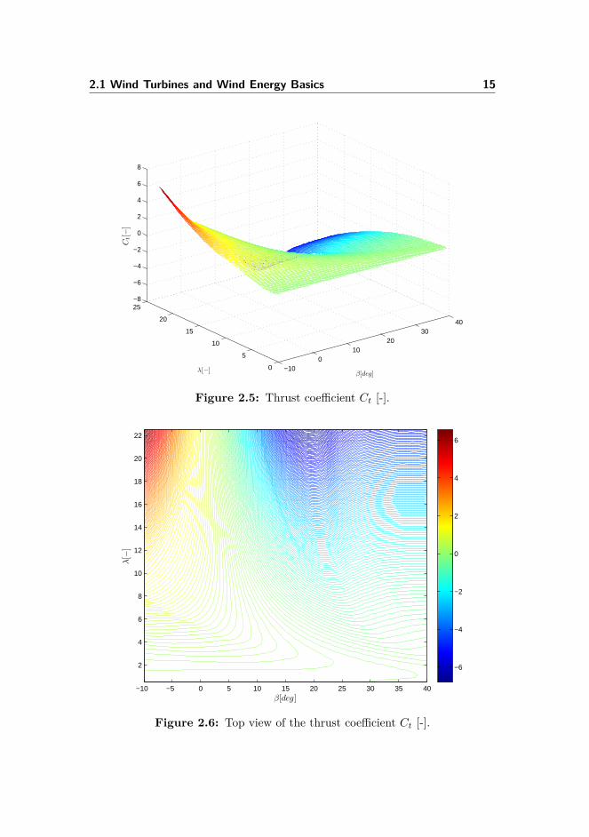
In figures 2.3 to 2.6 the curves of the power coefficient Cp and torque coefficientCt of the baseline wind turbine are shown in detail.
To transform the mechanical power extracted from the wind by the rotor, Pr,into electrical power Pe the power goes through many different components( thelow speed shaft, the gear box...) that have losses. Taking on account this fact,the electrical power is given by
Pe = ηPr (2.6)
where η is the efficiency factor. Without loss of generality η has been consideredequal to 1.
14 Modelling and Analysis
−100
1020
3040
0
5
10
15
20
250
0.1
0.2
0.3
0.4
0.5
β[deg]λ[−]
Cp[−
]
Figure 2.3: Power coefficient Cp [-].
β[deg]
λ[−
]
−10 −5 0 5 10 15 20 25 30 35 40
2
4
6
8
10
12
14
16
18
20
22
0.05
0.1
0.15
0.2
0.25
0.3
0.35
0.4
0.45
Figure 2.4: Top view of the power coefficient Cp [-].
2.1 Wind Turbines and Wind Energy Basics 15
−100
1020
3040
0
5
10
15
20
25−8
−6
−4
−2
0
2
4
6
8
β[deg]λ[−]
Ct[−]
Figure 2.5: Thrust coefficient Ct [-].
β[deg]
λ[−
]
−10 −5 0 5 10 15 20 25 30 35 40
2
4
6
8
10
12
14
16
18
20
22
−6
−4
−2
0
2
4
6
Figure 2.6: Top view of the thrust coefficient Ct [-].
16 Modelling and Analysis
2.2 Non-Linear Model
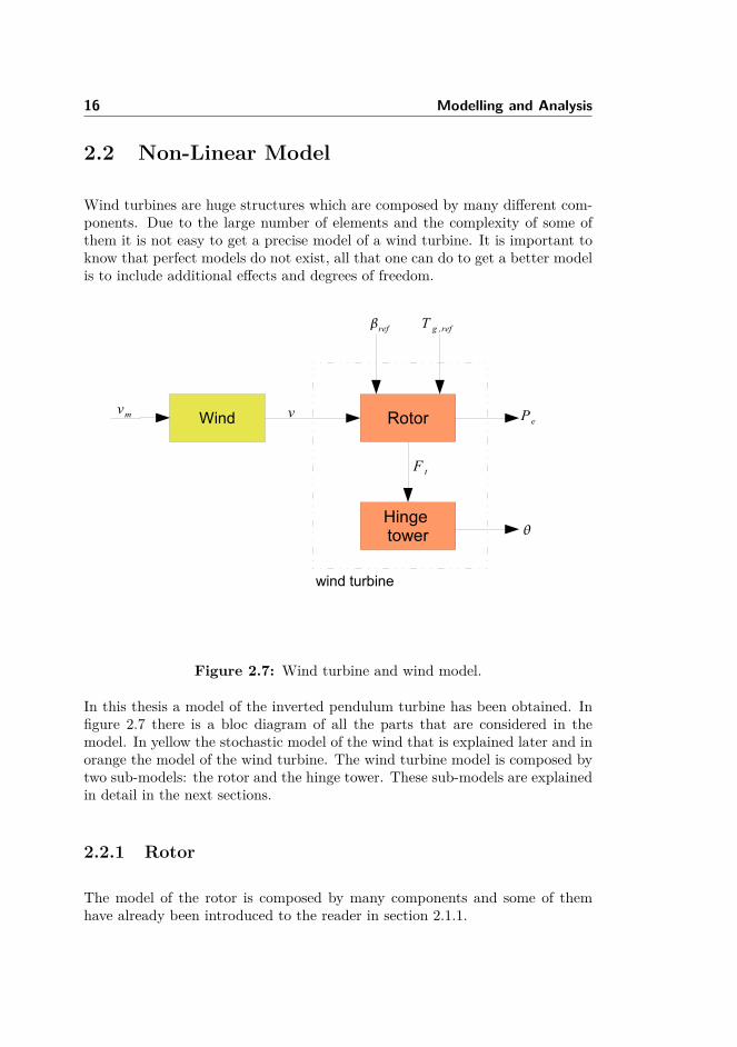
Wind turbines are huge structures which are composed by many different com-ponents. Due to the large number of elements and the complexity of some ofthem it is not easy to get a precise model of a wind turbine. It is important toknow that perfect models do not exist, all that one can do to get a better modelis to include additional effects and degrees of freedom.
Figure 2.7: Wind turbine and wind model.
In this thesis a model of the inverted pendulum turbine has been obtained. Infigure 2.7 there is a bloc diagram of all the parts that are considered in themodel. In yellow the stochastic model of the wind that is explained later and inorange the model of the wind turbine. The wind turbine model is composed bytwo sub-models: the rotor and the hinge tower. These sub-models are explainedin detail in the next sections.
2.2.1 Rotor
The model of the rotor is composed by many components and some of themhave already been introduced to the reader in section 2.1.1.

2.2 Non-Linear Model 17
The differential equation that models the dynamics of the rotor is
Jωr = Prωr−NTg (2.7)
This equation expresses the variation of the angular velocity. Using some of theformulas introduced in section 2.1.2 the equation 2.7 can be expressed as
Jωr = Tr −NTg = 1ωr
12ρaπR
2v3Cp −NTg (2.8)
It can be seen that the rotor dynamical equation is non-linear. Some of thenon-linearities are really complex, like the power coefficient Cp shown in figure2.3.
2.2.2 Hinge Tower
The idea of inverted pendulum turbine has already been introduced in section1.1 but a summary of the concept is done.
The peculiarity of the inverted pendulum turbine is the tower, which has a hingein its bottom. That hinge allows the turbine to balance forwards and backwardsand reduces the mechanical stress of the tower making it possible to have lighterand cheaper structure.
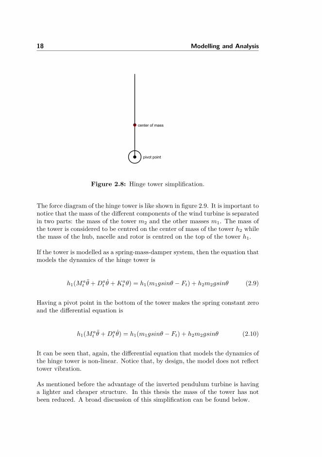
When modelling the inverted pendulum turbine, the tower has been consideredlike an inverted pendulum, with a pivot point in the bottom, a rigid stick andall the mass concentrated in the center of mass of the tower. Figure 2.8 helpsto understand the simplification made.
18 Modelling and Analysis
Figure 2.8: Hinge tower simplification.
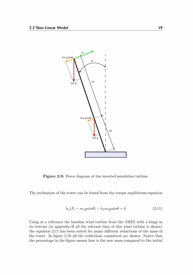
The force diagram of the hinge tower is like shown in figure 2.9. It is important tonotice that the mass of the different components of the wind turbine is separatedin two parts: the mass of the tower m2 and the other masses m1. The mass ofthe tower is considered to be centred on the center of mass of the tower h2 whilethe mass of the hub, nacelle and rotor is centred on the top of the tower h1.
If the tower is modelled as a spring-mass-damper system, then the equation thatmodels the dynamics of the hinge tower is
h1(Mat θ +Da
t θ +Kat θ) = h1(m1gsinθ − Ft) + h2m2gsinθ (2.9)
Having a pivot point in the bottom of the tower makes the spring constant zeroand the differential equation is
h1(Mat θ +Da
t θ) = h1(m1gsinθ − Ft) + h2m2gsinθ (2.10)
It can be seen that, again, the differential equation that models the dynamics ofthe hinge tower is non-linear. Notice that, by design, the model does not reflecttower vibration.
As mentioned before the advantage of the inverted pendulum turbine is havinga lighter and cheaper structure. In this thesis the mass of the tower has notbeen reduced. A broad discussion of this simplification can be found below.
2.2 Non-Linear Model 19
m1·g
m2·g
h2
h1
θ
m1·g·sinθ
m2·g·sinθ
Ft
Figure 2.9: Force diagram of the inverted pendulum turbine.
The inclination of the tower can be found from the torque equilibrium equation
h1(Ft −m1gsinθ)− h2m2gsinθ = 0 (2.11)
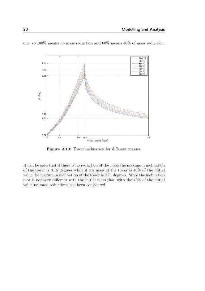
Using as a reference the baseline wind turbine from the NREL with a hinge inits bottom (in appendix B all the relevant data of this wind turbine is shown)the equation 2.11 has been solved for many different reductions of the mass ofthe tower. In figure 2.10 all the reductions considered are shown. Notice thatthe percentage in the figure means how is the new mass compared to the initial
20 Modelling and Analysis
one, so 100% means no mass reduction and 60% means 40% of mass reduction.
3 5.7 9.9 11.2 250.62
2.75
3.27
8.15
8.86
9.71
Wind speed [m/s]
θ[deg]
100 %90 %80 %70 %60 %50 %40 %
Figure 2.10: Tower inclination for different masses.
It can be seen that if there is no reduction of the mass the maximum inclinationof the tower is 8.15 degrees while if the mass of the tower is 40% of the initialvalue the maximum inclination of the tower is 9.71 degrees. Since the inclinationplot is not very different with the initial mass than with the 40% of the initialvalue no mass reductions has been considered.
2.3 Operation Modes and Steady State Analysis 21
2.3 Operation Modes and Steady State Analysis
2.3.1 Operation Regions Definition
Current wind turbines work in a specific wind speed range. The limits of theserange are known as cut-in and cut-out speed. As mentioned in (Burton et al.,2001) the cut-in speed is that wind speed at which the turbine starts to generatepower and the cut-out speed is when the turbine shuts-down to prevent itself tobe exposed to extreme loads. The latter might be subject to limitations due torequirements in each country’s grid codes.
The main objective of a wind turbines is to maximize the produced electricalpower. Notice that in this project the main objective is to avoid the collapseof the tower but maximizing the produced electrical power is also an importantobjective. So, for each wind speed in the range specified the electrical power ismaximized
max(Pe) = max(12ρaπR
2v3Cp(λ, β)) (2.12)
subject to
0 ≤ Pe ≤ Prated (2.13)
ωrmin≤ ωr ≤ ωrrated
(2.14)
These are some physical restrictions imposed by the generator that need to workin between some limits. Notice that, from the equation 2.12, to maximize thepower the only parameter that can be controlled is the Cp which depend on thepitch angle β and the tip speed ratio λ. Just as a remind the equation 2.3 ispresented again
λ = ωrR
v(2.15)
To achieve the goal of maximizing the power and holding the constrains imposedby the generator four regions are defined:
22 Modelling and Analysis
• Low region (I): In this region the rotational speed is kept at its lowestvalue ωrmin
while the power produced is maximized. For a given v the λis also given since the ωr is constant
λI = ωrminR
v(2.16)
Then to maximize the power the chosen β has to maximize the Cp. Theupper limit of this region is defined by
v1 = ωrminR
λ∗(2.17)
where λ∗ is the optimal tip speed ratio defined in the mid region by theequation 2.18.
• Mid region (II): In this region the power coefficient Cp is kept at ismaximum value, so the β and the λ are the optimal ones
(λ∗, β∗) = max(Cp(λ, β)) (2.18)
This generates a linear relation between the ωr and v
ωr = λ∗v
R(2.19)
The upper limit of this region is defined by
v2 = ωrratedR
λ∗(2.20)
• High region (III): In this region the ωr is kept at its rated value butnot the electrical power. For a given v the λ is defined
λIII = ωrratedR
v(2.21)
and the β is decide in order to maximize the electrical power. The upperlimit of this region is reached when the produced electrical power achievesits rated value.
• Top region (IV): In this region the electrical power is kept at its ratedvalue. For a given v the λ is defined
λIV = ωrratedR
v(2.22)
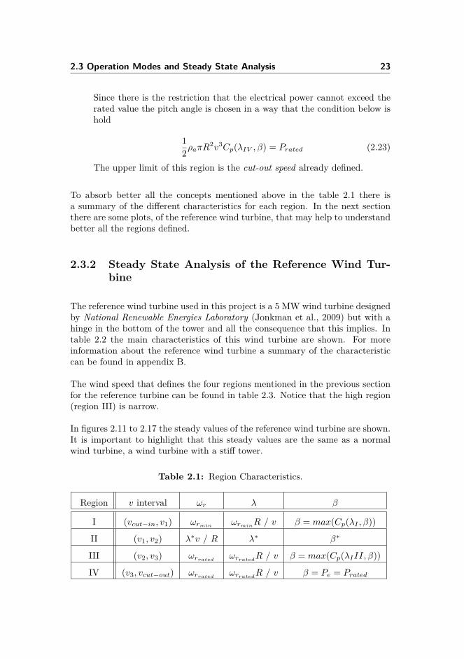
2.3 Operation Modes and Steady State Analysis 23
Since there is the restriction that the electrical power cannot exceed therated value the pitch angle is chosen in a way that the condition below ishold
12ρaπR
2v3Cp(λIV , β) = Prated (2.23)
The upper limit of this region is the cut-out speed already defined.
To absorb better all the concepts mentioned above in the table 2.1 there isa summary of the different characteristics for each region. In the next sectionthere are some plots, of the reference wind turbine, that may help to understandbetter all the regions defined.
2.3.2 Steady State Analysis of the Reference Wind Tur-bine
The reference wind turbine used in this project is a 5 MW wind turbine designedby National Renewable Energies Laboratory (Jonkman et al., 2009) but with ahinge in the bottom of the tower and all the consequence that this implies. Intable 2.2 the main characteristics of this wind turbine are shown. For moreinformation about the reference wind turbine a summary of the characteristiccan be found in appendix B.
The wind speed that defines the four regions mentioned in the previous sectionfor the reference turbine can be found in table 2.3. Notice that the high region(region III) is narrow.
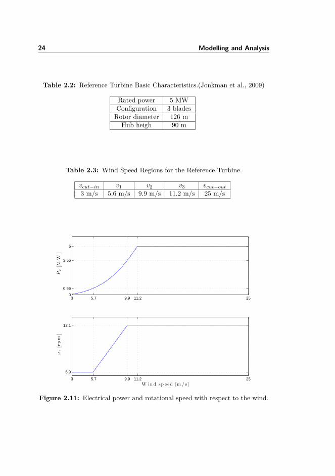
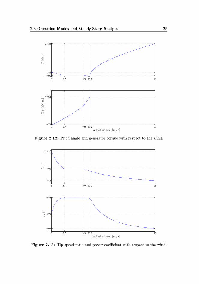
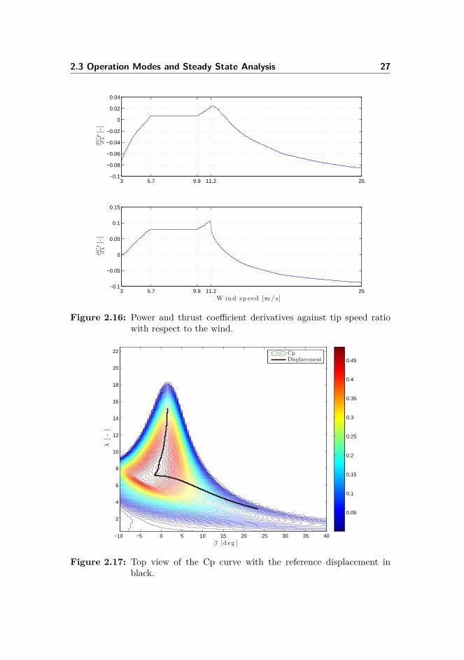
In figures 2.11 to 2.17 the steady values of the reference wind turbine are shown.It is important to highlight that this steady values are the same as a normalwind turbine, a wind turbine with a stiff tower.
Table 2.1: Region Characteristics.
Region v interval ωr λ β
I (vcut−in, v1) ωrmin ωrminR / v β = max(Cp(λI , β))
II (v1, v2) λ∗v / R λ∗ β∗
III (v2, v3) ωrratedωrrated
R / v β = max(Cp(λIII, β))
IV (v3, vcut−out) ωrratedωrrated
R / v β = Pe = Prated
24 Modelling and Analysis
Table 2.2: Reference Turbine Basic Characteristics.(Jonkman et al., 2009)
Rated power 5 MWConfiguration 3 bladesRotor diameter 126 m
Hub heigh 90 m
Table 2.3: Wind Speed Regions for the Reference Turbine.
vcut−in v1 v2 v3 vcut−out3 m/s 5.6 m/s 9.9 m/s 11.2 m/s 25 m/s
3 5.7 9.9 11.2 250
0.66
3.55
5
Pe[M
W]
3 5.7 9.9 11.2 25
6.9
12.1
W in d sp eed [m / s]
ωr[rpm
]
Figure 2.11: Electrical power and rotational speed with respect to the wind.
2.3 Operation Modes and Steady State Analysis 25
3 5.7 9.9 11.2 25
−0.911.48
23.33β
[deg]
3 5.7 9.9 11.2 250.73
40.68
W in d sp eed [m / s]
Tg
[kN
m]
Figure 2.12: Pitch angle and generator torque with respect to the wind.
3 5.7 9.9 11.2 25
3.19
8.06
15.17
λ[-]
3 5.7 9.9 11.2 25
0.04
0.25
0.49
W in d sp eed [m / s]
Cp[-]
Figure 2.13: Tip speed ratio and power coefficient with respect to the wind.

26 Modelling and Analysis
3 5.7 9.9 11.2 25
0.06
0.85
Ct[-]
3 5.7 9.9 11.2 25
59.14
260.88
770.92
W in d sp eed [m / s]
Ft[k
N]
Figure 2.14: Thrust coefficient and thrust force with respect to the wind.
3 5.7 9.9 11.2 25−0.04
−0.03
−0.02
−0.01
0
0.01
∂C
p∂β
[-]
3 5.7 9.9 11.2 25−0.2
−0.15
−0.1
−0.05
0
W in d sp eed [m / s]
∂C
t∂β
[-]
Figure 2.15: Power and thrust coefficient derivatives against pitch with re-spect to the wind.
2.3 Operation Modes and Steady State Analysis 27
3 5.7 9.9 11.2 25−0.1
−0.08
−0.06
−0.04
−0.02
0
0.02
0.04∂C
p∂λ
[-]
3 5.7 9.9 11.2 25−0.1
−0.05
0
0.05
0.1
0.15
W in d sp eed [m / s]
∂C
t∂λ
[-]
Figure 2.16: Power and thrust coefficient derivatives against tip speed ratiowith respect to the wind.
−10 −5 0 5 10 15 20 25 30 35 40
2
4
6
8
10
12
14
16
18
20
22
β [d eg ]
λ[-]
0.05
0.1
0.15
0.2
0.25
0.3
0.35
0.4
0.45CpDisplacement
Figure 2.17: Top view of the Cp curve with the reference displacement inblack.
28 Modelling and Analysis
3 5.7 9.9 11.2 250.62
2.75
8.15
Wind speed [m/s]
θ[deg]
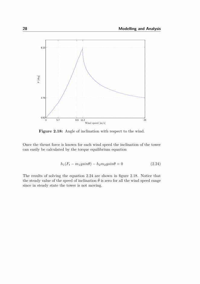
Figure 2.18: Angle of inclination with respect to the wind.
Once the thrust force is known for each wind speed the inclination of the towercan easily be calculated by the torque equilibrium equation
h1(Ft −m1gsinθ)− h2m2gsinθ = 0 (2.24)
The results of solving the equation 2.24 are shown in figure 2.18. Notice thatthe steady value of the speed of inclination θ is zero for all the wind speed rangesince in steady state the tower is not moving.

2.4 Linear Model 29
2.4 Linear Model
In this section the linear model of the inverted pendulum turbine and of thestochastic wind are explained.
2.4.1 Wind Turbine Model
The complete model of the inverted pendulum turbine is a third order systemwhich differential dynamical equations are
Jωr = Tr −NTg (2.25)
h1(Mat θ +Da
t θ) = h1(m1gsinθ − Ft) + h2m2gsinθ (2.26)
Using as a states
x =
ωrθ
θ
(2.27)
as an inputs
u =[βTg
](2.28)
as a measurements or outputs
y =
Peωrθ
(2.29)
and as a disturbance the wind speed v the non-linear system can be expressed
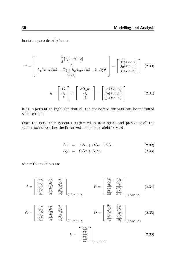
30 Modelling and Analysis
in state space description as
x =
1J
[Tr −NTg]θ
h1(m1gsinθ − Ft) + h2m2gsinθ − h1Dat θ
h1Mat
=
f1(x, u, v)f2(x, u, v)f3(x, u, v)
(2.30)
y =
Peωrθ
=
NTgωrωrθ
=
g1(x, u, v)g2(x, u, v)g3(x, u, v)
(2.31)
It is important to highlight that all the considered outputs can be measuredwith sensors.
Once the non-linear system is expressed in state space and providing all thesteady points getting the linearized model is straightforward
∆x = A∆x+B∆u+ E∆v (2.32)∆y = C∆x+D∆u (2.33)
where the matrices are
A =
∂f1∂ωr
∂f1∂θ
∂f1∂θ
∂f2∂ωr
∂f2∂θ
∂f2∂θ
∂f3∂ωr
∂f3∂θ
∂f3∂θ
(x∗,u∗,v∗)
B =
∂f1∂β
∂f1∂Tg
∂f2∂β
∂f2∂Tg
∂f3∂β
∂f3∂Tg
(x∗,u∗,v∗)
(2.34)
C =
∂g1∂ωr
∂g1∂θ
∂g1∂θ
∂g2∂ωr
∂g2∂θ
∂g2∂θ
∂g3∂ωr
∂g3∂θ
∂g3∂θ
(x∗,u∗,v∗)
D =
∂g1∂β
∂g1∂Tg
∂g2∂β
∂g2∂Tg
∂g3∂β
∂g3∂Tg
(x∗,u∗,v∗)
(2.35)
E =
∂f1∂v∂f2∂v∂f3∂v
(x∗,u∗,v∗)
(2.36)
2.4 Linear Model 31
and vectors are
∆x = x− x∗ ∆x = x− x∗ ∆u = u− u∗ (2.37)
∆v = v − v∗ ∆y = y − y∗ (2.38)
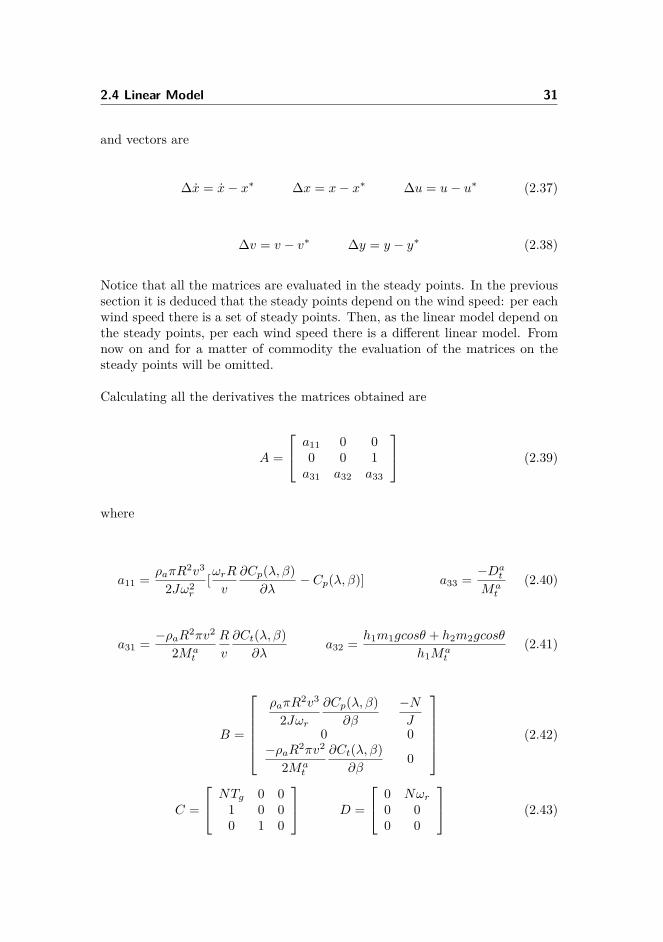
Notice that all the matrices are evaluated in the steady points. In the previoussection it is deduced that the steady points depend on the wind speed: per eachwind speed there is a set of steady points. Then, as the linear model depend onthe steady points, per each wind speed there is a different linear model. Fromnow on and for a matter of commodity the evaluation of the matrices on thesteady points will be omitted.
Calculating all the derivatives the matrices obtained are
A =
a11 0 00 0 1a31 a32 a33
(2.39)
where
a11 = ρaπR2v3
2Jω2r
[ωrRv
∂Cp(λ, β)∂λ
− Cp(λ, β)] a33 = −Dat
Mat
(2.40)
a31 = −ρaR2πv2
2Mat
R
v
∂Ct(λ, β)∂λ
a32 = h1m1gcosθ + h2m2gcosθ
h1Mat
(2.41)
B =
ρaπR
2v3
2Jωr∂Cp(λ, β)
∂β
−NJ
0 0−ρaR2πv2
2Mat
∂Ct(λ, β)∂β
0
(2.42)
C =
NTg 0 01 0 00 1 0
D =
0 Nωr0 00 0
(2.43)
32 Modelling and Analysis
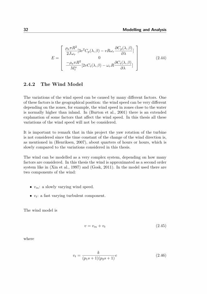
E =
ρaπR
2
2Jωr[3v2Cp(λ, β)− vRωr
∂Cp(λ, β)∂λ
]0
−ρaπR2
Mat
[2vCt(λ, β)− ωrR∂Ct(λ, β)
∂λ]
(2.44)
2.4.2 The Wind Model
The variations of the wind speed can be caused by many different factors. Oneof these factors is the geographical position: the wind speed can be very differentdepending on the zones, for example, the wind speed in zones close to the wateris normally higher than inland. In (Burton et al., 2001) there is an extendedexplanation of some factors that affect the wind speed. In this thesis all thesevariations of the wind speed will not be considered.
It is important to remark that in this project the yaw rotation of the turbineis not considered since the time constant of the change of the wind direction is,as mentioned in (Henriksen, 2007), about quarters of hours or hours, which isslowly compared to the variations considered in this thesis.
The wind can be modelled as a very complex system, depending on how manyfactors are considered. In this thesis the wind is approximated as a second ordersystem like in (Xin et al., 1997) and (Gosk, 2011). In the model used there aretwo components of the wind:
• vm: a slowly varying wind speed.
• vt: a fast varying turbulent component.
The wind model is
v = vm + vt (2.45)
where
vt = k
(p1s+ 1)(p2s+ 1)e (2.46)
2.4 Linear Model 33
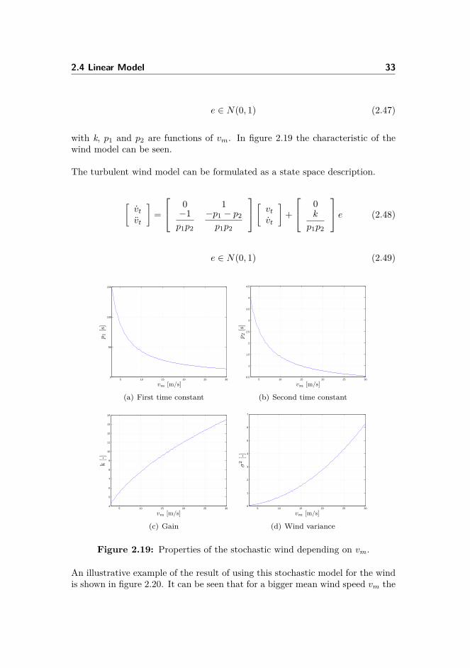
e ∈ N(0, 1) (2.47)
with k, p1 and p2 are functions of vm. In figure 2.19 the characteristic of thewind model can be seen.
The turbulent wind model can be formulated as a state space description.
[vtvt
]=
0 1−1p1p2
−p1 − p2
p1p2
[ vtvt
]+
0k
p1p2
e (2.48)
e ∈ N(0, 1) (2.49)
5 10 15 20 25 300
50
100
150
p 1[s]
vm [m/s]
(a) First time constant
5 10 15 20 25 300.5
1
1.5
2
2.5
3
3.5
4
4.5
p 2[s]
vm [m/s]
(b) Second time constant
5 10 15 20 25 304
5
6
7
8
9
10
11
12
13
14
k[-]
vm [m/s]
(c) Gain
5 10 15 20 25 300
1
2
3
4
5
6
7
σ2[-]
vm [m/s]
(d) Wind variance
Figure 2.19: Properties of the stochastic wind depending on vm.
An illustrative example of the result of using this stochastic model for the windis shown in figure 2.20. It can be seen that for a bigger mean wind speed vm the

34 Modelling and Analysis
variation of the wind increases as shown in figure 2.19. This difference betweenvariances can be appreciated because both wind data have been generated withthe same random numbers.
0 20 40 60 80 100 120 140 160 180 2006
8
10
12
14
16
18
20
Time [s]
Windspeed[m
/s]
vm = 15m/svm = 7m/s
Figure 2.20: Illustrative example of the stochastic wind model.
2.4.3 Affine Model
The linear model presented in the previous section is expressed in deviationvariables(also called relative or incremental). From now on and for a matter ofcomfortingly the system is expressed in affine way. That way all the variablesare in absolute values and there is no need to add or subtract the steady states.The procedure how to get the affine model from the deviation one is done inequations 2.50 to 2.55 as shown in (Gosk, 2011).
x− x∗ = A(x− x∗) +B(u− u∗) + E(v − v∗) (2.50)
y − y∗ = C(x− x∗) +D(u− u∗) (2.51)

2.4 Linear Model 35
Organizing all the steady values it can be obtained
x = Ax+Bu+ Ev−Ax∗ −Bu∗ − Ev∗ + x∗︸ ︷︷ ︸dx
(2.52)
y = Cx+Du−Cx∗ −Du∗ + y∗︸ ︷︷ ︸dy
(2.53)
then the system can be expressed like
x = Ax+Bu+ Ev + dx (2.54)
y = Cx+Du+ dy (2.55)

36 Modelling and Analysis
2.5 Model Analysis
In this section the characteristic of the model obtained are studied and the linearmodel obtained is compared with the non-linear one to verify its behaviour.
2.5.1 Characteristics of the System
2.5.1.1 Stability
The inverted pendulum turbine is inspired in the typical control problem of theinverted pendulum. It is well known that the inverted pendulum is an unstablesystem and it sounds reasonable that the inverted pendulum turbine may alsobe unstable.
From (Slotine and Li, 1991) it is known that given a a non-linear system, likethe current case, the stability of this system can be discussed from the lineariza-tion state space description. This method is known as Lyapunov’s linearizationmethod. Depending on the eigenvalues of the linearized state space system ma-trix the stability of the system can be discussed as follows
• If Re(λi) < 0 ∀i → The non-linear system is local asymptotic stable.
• If ∃ λi|Re(λi)>0 → The non-linear system is unstable.
• If ∃ λi|Re(λi)=0 → Nothing can be said about the stability of the non-linearsystem.
So with a look at the eigenvalue of the space state description it can easily bearout the instability of the system.
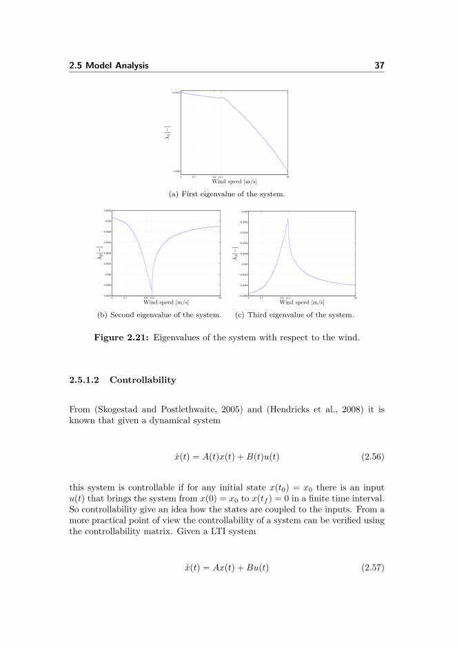
From figure 2.21 it can be seen that one eigenvalue, λ2, is positive in the wholerange of wind speed and the instability is now verified.
Having an unstable system sound reasonable because
• If the angle of inclination is bigger than the steady value then the towerwould fall forward since the gravity force is higher than the thrust force.
• If the angle of inclination is lower than the steady value then the towerwould fall backwards since the thrust force is higher than the gravity force.
2.5 Model Analysis 37
3 5.7 9.9 11.2 25
−0.526
−0.0121
Wind speed [m/s]
λ1[−
]
(a) First eigenvalue of the system.
3 5.7 9.9 11.2 250.2616
0.2618
0.262
0.2622
0.2624
0.2626
0.2628
0.263
0.2632
Wind speed [m/s]
λ2[−
]
(b) Second eigenvalue of the system.
3 5.7 9.9 11.2 25−0.3046
−0.3044
−0.3042
−0.304
−0.3038
−0.3036
−0.3034
−0.3032
−0.303
Wind speed [m/s]
λ3[−
]
(c) Third eigenvalue of the system.
Figure 2.21: Eigenvalues of the system with respect to the wind.
2.5.1.2 Controllability
From (Skogestad and Postlethwaite, 2005) and (Hendricks et al., 2008) it isknown that given a dynamical system
x(t) = A(t)x(t) +B(t)u(t) (2.56)
this system is controllable if for any initial state x(t0) = x0 there is an inputu(t) that brings the system from x(0) = x0 to x(tf ) = 0 in a finite time interval.So controllability give an idea how the states are coupled to the inputs. From amore practical point of view the controllability of a system can be verified usingthe controllability matrix. Given a LTI system
x(t) = Ax(t) +Bu(t) (2.57)

38 Modelling and Analysis
the controllability matrix is defined as follows
Mc =[B AB A2B ... AnB
](2.58)
The system 2.57 is controllable ifMc is full rank. The inverted pendulum turbinehas been proved to be controllable since the controllability matrix is full rankfor all the wind speed range.
2.5.1.3 Observability
From (Skogestad and Postlethwaite, 2005) and (Hendricks et al., 2008) it isknown that given a dynamical system
x(t) = A(t)x(t) +B(t)u(t) (2.59)
y(t) = C(t)x(t) +D(t)u(t) (2.60)
this system is observable on the finite time interval [t0, tf ] if any initial state x0is uniquely determined by the output y(t) over the same time interval. From amore practical point of view the observability of a system can be verified usingthe observability matrix. Given a LTI system
x(t) = Ax(t) +Bu(t) (2.61)
y(t) = Cx(t) +Du(t) (2.62)
the observability matrix is defined as follows
Mo =
CCACA2
...CAn−1
(2.63)
The system 2.61 and 2.62 is observable if Mo is full rank. The observability ofthe inverted pendulum turbine has been verified since the rank of the Mo is 3in all the wind interval.
2.5 Model Analysis 39
2.5.2 Model Verification
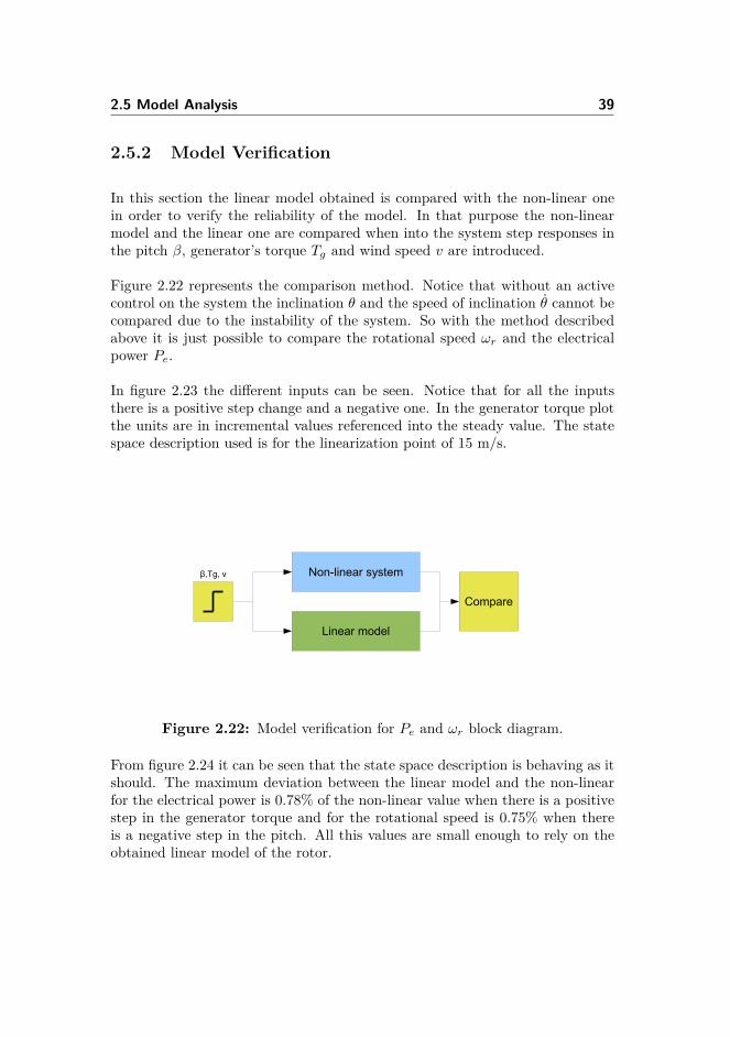
In this section the linear model obtained is compared with the non-linear onein order to verify the reliability of the model. In that purpose the non-linearmodel and the linear one are compared when into the system step responses inthe pitch β, generator’s torque Tg and wind speed v are introduced.
Figure 2.22 represents the comparison method. Notice that without an activecontrol on the system the inclination θ and the speed of inclination θ cannot becompared due to the instability of the system. So with the method describedabove it is just possible to compare the rotational speed ωr and the electricalpower Pe.
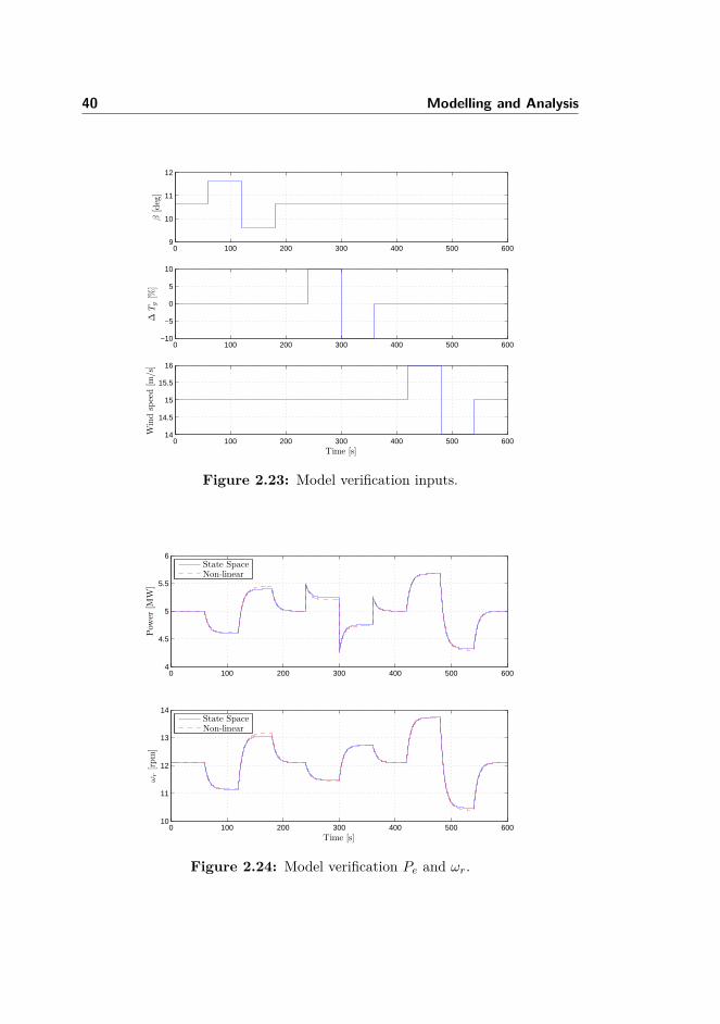
In figure 2.23 the different inputs can be seen. Notice that for all the inputsthere is a positive step change and a negative one. In the generator torque plotthe units are in incremental values referenced into the steady value. The statespace description used is for the linearization point of 15 m/s.
Figure 2.22: Model verification for Pe and ωr block diagram.
From figure 2.24 it can be seen that the state space description is behaving as itshould. The maximum deviation between the linear model and the non-linearfor the electrical power is 0.78% of the non-linear value when there is a positivestep in the generator torque and for the rotational speed is 0.75% when thereis a negative step in the pitch. All this values are small enough to rely on theobtained linear model of the rotor.
40 Modelling and Analysis
0 100 200 300 400 500 6009
10
11
12
β[deg]
0 100 200 300 400 500 600−10
−5
0
5
10
∆Tg[%
]
0 100 200 300 400 500 60014
14.5
15
15.5
16
Windspeed[m
/s]
Time [s]
Figure 2.23: Model verification inputs.
0 100 200 300 400 500 6004
4.5
5
5.5
6
Pow
er[M
W]
State SpaceNon-linear
0 100 200 300 400 500 60010
11
12
13
14
ωr[rpm]
Time [s]
State SpaceNon-linear
Figure 2.24: Model verification Pe and ωr.
2.5 Model Analysis 41
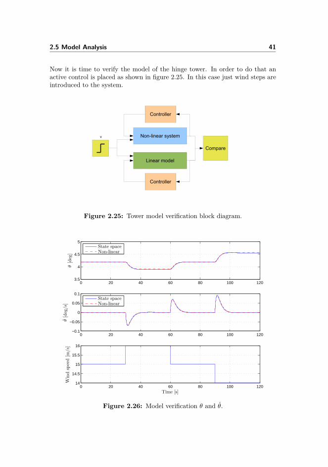
Now it is time to verify the model of the hinge tower. In order to do that anactive control is placed as shown in figure 2.25. In this case just wind steps areintroduced to the system.
Figure 2.25: Tower model verification block diagram.
0 20 40 60 80 100 1203.5
4
4.5
5
θ[deg]
State spaceNon-linear
0 20 40 60 80 100 120−0.1
−0.05
0
0.05
0.1
θ[deg/s]
State spaceNon-linear
0 20 40 60 80 100 12014
14.5
15
15.5
16
Windspeed[m
/s]
Time [s]
Figure 2.26: Model verification θ and θ.

42 Modelling and Analysis
From figure 2.26 it can be seen that the model of the tower is behaving properly.The maximum deviation between the linear model and the non-linear one for θis 0.4% of the non-linear value when a positive step in the wind is done, whilein θ is 3% of the non-linear value when there is a negative step in the wind.In this last case the deviation is a little bit bigger since the values of the speedof inclination are very small. All this values are small enough to rely on theobtained linear model of the hinge tower.

Chapter 3
Control Methods
In this chapter all the control theory used in the realization of this project isexplained. The reader should no expect a large and broad discussion of all theconcepts introduced.
3.1 Kalman Filter
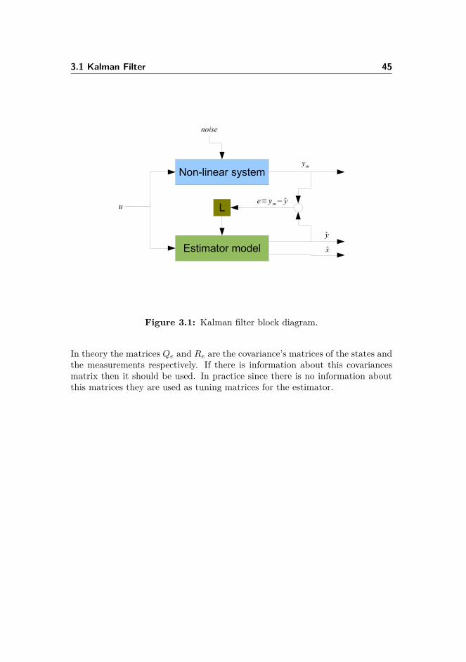
In this section it is shown the theory behind the estimation of the states, x, byobserving the outputs y with an optimal observer: a Kalman Filter.
In real applications almost all the measurements done have some errors. This iscaused because the states or their measurement may be corrupted by some kindof noise. In that situation it becomes very useful an optimal estimator, like theKalman filter, that is able to estimate the states with the noisy measurementsof them.
The formulation of the optimal observer is done in discrete time but it can alsobe done in continuous time. This approach is described in detail in (Hendrickset al., 2008).
Before starting the explanation some nomenclature notes should be done:

44 Control Methods
• The symbol ’ ˆ ’ means estimated value. So x is the estimated value of xand y is the estimated value of y.
• ym is the measured output from the real plant.
• xk|k−1 is the estimated value of x for the sample k with the data from thesample k − 1.
• L is the Kalman gain matrix.
Given the LTI system in discrete time
xk+1 = Axk +Buk + wk (3.1)
yk = Cxk +Duk + vk (3.2)
where wk is the state noise and vk is the measurements noise. Both, wk and vkare white noise, uncorrelated and normally distributed with zero mean
wk ∈ N(0, Qe) (3.3)
vk ∈ N(0, Re) (3.4)
The steady-state Kalman filter is able to estimate the state in two steps thedata update, equation 3.5, and the time update, equation 3.6,
xk|k = xk|k−1 + L(ym − (Cxk|k−1 +Duk)︸ ︷︷ ︸y
) (3.5)
xk+1|k = Axk|k +Buk (3.6)
For a better understanding of how the Kalman filter works in figure 3.1 there ishelpful block diagram.
3.1 Kalman Filter 45
Figure 3.1: Kalman filter block diagram.
In theory the matrices Qe and Re are the covariance’s matrices of the states andthe measurements respectively. If there is information about this covariancesmatrix then it should be used. In practice since there is no information aboutthis matrices they are used as tuning matrices for the estimator.

46 Control Methods
3.2 Linear Quadratic Regulator
In this section a solution to the standard regulation problem and the mostcommon version of it, the Linear Quadratic Regulator, are presented. In thisformulation the cost function is quadratic in the states and the inputs.
From (Hendricks et al., 2008), given a non-linear n-dimensional system like
x(t) = f(x(t), u(t), t) (3.7)
with the initial condition
x(t0) = x0 (3.8)
The objective is to optimize the control in a finite time interval [t0, t1]. In orderto achieve that goal the performance index is presented
J(u) = Φ(x(t1), t1) +∫ t1
t0
L(x(t), u(t), t)dt (3.9)
The performance index is composed by two terms. The first term of equation 3.9is a function that depends on the final state. The second term of the equation3.9 is a function that depends on the states and the inputs vectors, also calledcost function. The performance index give an idea of the quality of the controlaction defined: a large value of J means a bad control while a small value of Ja good control.
The general optimal control problem is try to find a control action u(t) for ainterval [t0, t1] that minimizes the performance index J.
The linear quadratic regulator is the most common formulation for regulationoptimal control problem. The LQR problem is presented in discrete time butit can also be formulated in continuous time. For a more generic formulationthe cross terms on the cost function are also considered. In (Poulsen, 2012a)there is a detailed demonstration how to solve the minimization problem buthere this is not going to be developed, just the results of it are shown.
3.2 Linear Quadratic Regulator 47
Given the LTI system in discrete time
xk+1 = Axk +Buk (3.10)
with the initial condition
x|k=0 = x0 (3.11)
the cost function to minimize in a finite horizon N is
J = xTNPxN +N−1∑k=0
xTkQxk + uTkRuk + 2xTkNuk (3.12)
While minimizing the cost function a recursive discrete time Ricatti equationneeds to be solved
Sk = Q+ATSk+1A−(ATSk+1B+N)(BTSk+1B+R)−1(BTSk+1A+NT ) (3.13)
With the solution of equation 3.13 the optimal control law is found
uk = −Kkxk (3.14)
with the gain matrix
Kk = (BTSk+1B +R)−1(BTSk+1A+NT ) (3.15)
The development mentioned above is valid for a finite time horizon. The sameresults can be extrapolated for a infinite horizon. The Riccati equation to solveis now
0 = Q+ATSA− (ATSB +N)(BTSB +R)−1(BTSA+NT )− S (3.16)

48 Control Methods
The optimal feedback gain matrix is then
K = (BTSB +R)−1(BTSA+NT ) (3.17)
In the formulation of the cost function 3.12 there are three weight matrices,Q, R and N . Having a high weight in a specific variable put more priority atthe minimization of that variable than the others while having a low or zeroweight in a variable means that the minimization of the specific variable is notimportant.
In (Franklin et al., 2002) there is a mention to Bryson’s rule, which give a firstchoice for the matrices Q, R and N
Qii = 1maximum acceptable value of x2
i
(3.18)
Rjj = 1maximum acceptable value of u2
j
(3.19)
Nij = 1maximum acceptable value of xiuj
(3.20)
3.3 Linear Quadratic Gaussian Control 49
3.3 Linear Quadratic Gaussian Control
In this section it is presented a control method that uses a Linear QuadraticRegulator and a Kalman filter all together, this kind of control is known asLinear Quadratic Gaussian Control.
The name of LQG comes from the use of a Linear model, a Quadratic costfunction and a Gaussian white process noise to model disturbances and noise.A broad discussion of LQG can be found in (Skogestad and Postlethwaite, 2005).The approach below is done in discrete time but it could be done in continuoustime.
Given a LTI system with Gaussian white process noise in the states and mea-surements
xk+1 = Axk +Buk + wk (3.21)
yk = Cxk +Duk + vk (3.22)
First of all an optimal controller, a Linear Quadratic Regulator, for the linearsystem above without the Gaussian noise vk and ek needs to be found
u(t) = −Kx(t) (3.23)
The gain matrix K is found with the techniques mentioned in the previoussection 3.2.
Once the optimal controller is designed and optimal estimator is used for esti-mating the states with the measurements. To achieve that goal a Kalman filteris used. Finally the estimation x is substituted in the control action
u(t) = −Kx(t) (3.24)
As it can be seen, the LQG is a pure application of the separation theoremsince it is possible to assign the eigenvalues from the state feedback and theeigenvalues from the estimator separately.
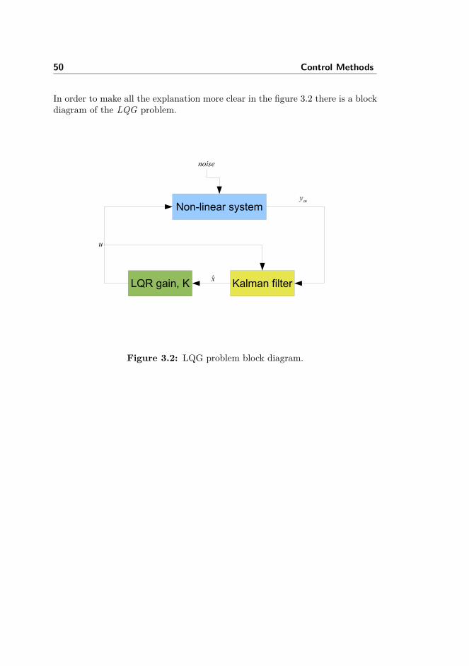
50 Control Methods
In order to make all the explanation more clear in the figure 3.2 there is a blockdiagram of the LQG problem.
Figure 3.2: LQG problem block diagram.

3.4 Offset-Free Methods 51
3.4 Offset-Free Methods
In this section two methods to achieve offset free performance are presented.The first method gets zero offset integrating the difference between the referencevalue and the real value while the other method introduced disturbances to themodel to get offset free performance.
3.4.1 Integral Action
The most easy and old way to get zero offset performance is using an integratorthat eliminates the difference between the real and the reference value. Whenusing integrators one have to be aware of their tendency to destabilise a system.
In this project the viability of using an integral action over a LQR problem hasbeen carried out. In (Kedjar and Al-Haddad, 2009) a broad explanation of thelinear quadratic regulator with integral action, LQI, can be found.
Given the LTI system in discrete time
xk+1 = Axk +Buk (3.25)
yk = Cxk +Duk (3.26)
an integral action to the state xi is defined
ek+1 = ek + (xi,k − xi,ref ) (3.27)
Then, if the equation 3.27 is added to 3.25 it can be obtained
[xk+1ek+1
]=[A 00 I
] [xkek
]+[B0
]uk +
[0
xi,k − xi,ref
](3.28)
Using also the equation 3.26 the expression above can be reformulated as
[xk+1ek+1
]=[
A 0C|xi
I
] [xkek
]+[
BD|xi
]uk +
[0
−xi,ref
](3.29)
52 Control Methods
3.4.2 Disturbance Modelling
Another technique to achieve offset-free performance is to add integrating dis-turbances to the process model. The aim of adding this disturbances is toeliminate the mismatch between the model and the plant but also the unmea-sured disturbances. A broad discussion of the disturbance modelling techniqueis found in (Pannocchia and Rawlings, 2003) and (Muske and Badgwell, 2002).
The main idea of the disturbance modelling is that the disturbances added tothe system absorb any mismatch until zero offset is achieved. The first step tofollow when implementing this offset free technique is to add disturbances to thesystem, afterwards the states and the disturbances are estimated using a Kalmanfilter designed for the augmented system. When the control loop is closed thedisturbances estimations are use to achieve the zero offset performance.
Given the LTI system in discrete time with Gaussian noise
xk+1 = Axk +Buk + wk (3.30)
yk = Cxk +Duk + vk (3.31)
The disturbances can be placed either in the states, also called inputs distur-bances,
xk+1 = Axk +Buk +Bddk + wk (3.32)
dk+1 = dk + wkd(3.33)
either in the measurements, also called outputs disturbances,
yk = Cxk +Duk + Cdpk + vk (3.34)
pk+1 = pk + vkp (3.35)

3.4 Offset-Free Methods 53
either in both states and measurements
xk+1dk+1pk+1
=
A Bd 00 I 00 0 I
xkdkpk
+
B00
uk +
wkwkd
vkp
(3.36)
yk =[C 0 Cd
] xkdkpk
+Duk + vkp(3.37)
where the wkdand vkp
are the noise of the input and output disturbances re-spectively.
As mentioned in (Pannocchia and Rawlings, 2003) there are some considerationsto take in account to success with the disturbance modelling technique. First ofall the augmented system has to be detectable. The detectability of a system isa slightly weaker notion than observability: a system is detectable if and onlyif all of its unobservable modes are stable. This condition is held if and only if
• The non-augmented system is detectable.
• If the condition below is hold
rank
[A− I Bd 0C 0 Cd
]= nx + nd (3.38)
That implies that the maximum number of disturbances that can be added tothe system is equal to the number of measurements
nd ≤ ny (3.39)
Deciding the structure of the augmented system is not an easy task. There aremany things to take in account:
• The number of disturbances.
• Where to place the disturbances in the states and/or in the measurements.
• Chose the appropriate matrices Bd and Cd.
• Check that the conditions mentioned earlier hold.

54 Control Methods
This is a trial-error method until zero offset performance is achieved. When oneaccomplish this goal the augmented system is properly designed.

Chapter 4
Implementation and Results
In this chapter the controller implemented and all the results from the simu-lations are shown. All the control techniques used have been explained in theprevious chapter.
First of all the baseline controller implemented by NREL in (Jonkman et al.,2009) is explained. Then the control strategy of the implemented controller isexposed and afterwards the results of this control action are shown. Finally theperformance of the controller designed over the inverted pendulum turbine iscompared with a wind turbine with a stiff tower.
4.1 Baseline Controller
Current wind turbines use quite simple controllers. In this section the baselinecontroller designed by NREL is explained.
The main control objective of the baseline controller is to control the producedelectrical power. To achieve that goal two independent controllers are imple-mented: a generator torque controller and a pitch angle controller.

56 Implementation and Results
Figure 4.1: Baseline controller flowchart.
The generator torque controller is responsible of controlling the power produc-tion below the critical wind speed. The critical wind speed is the one in betweenthe high region (III) and the top region (IV) defined in section 2.3.1 as v3. Thecontrol action of this controller works with a lookup table. Depending on thepitch value and the generator speed the controller identifies the current regionand applies the relevant generator torque. Above the critical wind speed thegenerator torque is kept constant.
The pitch angle controller is responsible of controlling the power produced abovethe critical wind speed. This is a PI controller with gain scheduling designed onthe first order model of the wind turbine. The controller input is the differencebetween the real generator speed and the rated referenced generator speed.Depending on the pitch angle the gain of the PI controller changes. Below thecritical wind speed the pitch angle is kept constant.
In figure 4.1 there is a block diagram of the baseline controller to help to under-stand how does it work. It is important to notice that this is a basic explanationof the baseline controller and some of the control details have been omitted. In(Jonkman et al., 2009) there is a detailed explanation of a baseline controllerfor the 5-MW reference wind turbine.

4.2 Control Strategy 57
4.2 Control Strategy
The inverted pendulum turbine is an unstable system as demonstrated in section2.5.1.1. The control objectives of the inverted pendulum turbine are a littlebit different from other wind turbines. The main control objective is to keepthe tower still, in a suitable inclination. Once the first control objective isaccomplished the other goal to achieve is the maximization of the producedelectrical power.
In section 2.3 the criteria of how to get the steady state points is explained.The steady states points have been chosen with the aim of maximize the elec-trical power, like other wind turbines. Once the steady points have been foundthe inclination of the tower has been chosen accordingly. The criteria followedensures the maximization of the electrical power.
4.2.1 Control Objectives per Region
Each one of the four regions defined has different control objectives. In thissection the control designed for each region is explained.
It is important to notice that in the baseline controller the pitch is kept in aconstant value for region I, II and III. This is due to the fact that, between otherreasons, the pitch component of the input matrix B is zero since the derivativeof the Cp against the pitch angle β is zero.
In the inverted pendulum turbine the pitch component of the input matrix isnot zero since the derivative of the Ct curve against the pitch β is not zero. Theplots of the derivatives of the Cp and Ct against β and λ are shown in 2.15 and2.16.
B =
ρaπR
2v3
2Jωr∂Cp(λ, β)
∂β
−NJ
0 0−ρaR2πv2
2Mat
∂Ct(λ, β)∂β
0
(4.1)
Low region (I)
In this region the rotation speed is kept in its lowest level while the producedelectrical power is maximized. Notice that the criterion followed in the base-
58 Implementation and Results
line controller, keeping the pitch angle fixed, cannot be applied in the invertedpendulum turbine. If the pitch is fixed in an certain angle there is no action tokeep the tower in an appropriate inclination. So the reference introduced to thesystem is
r =
ωrθ
θ
=
ωrmin
θref0
(4.2)
Mid region (II)
In region II the objective is to maximize the produced electrical power by tryingto keep the wind turbine on the top part of the Cp curve. In order to achievethis goal the pitch reference is kept at the optimal point β∗ and the ωr is chosenin a way that the λ is kept at its optimal point λ∗.
r =
ωrθ
θ
=
λ∗vRθref
0
(4.3)
High region (III)
In region III the rotational speed reference is kept at its rated value. Since thisregion is really narrow it has been used for a transition between regions II andIV.
r =
ωrθ
θ
=
ωrrated
θref0
(4.4)
Top region (IV)
In region IV the rotational speed reference is kept at its rated value as thegenerator torque. Since the objective is to keep the produced electrical powerat its rated value the reference pitch angle is increasing, this action is known aspitching out.
r =
ωrθ
θ
=
ωrrated
θref0
(4.5)
4.2 Control Strategy 59
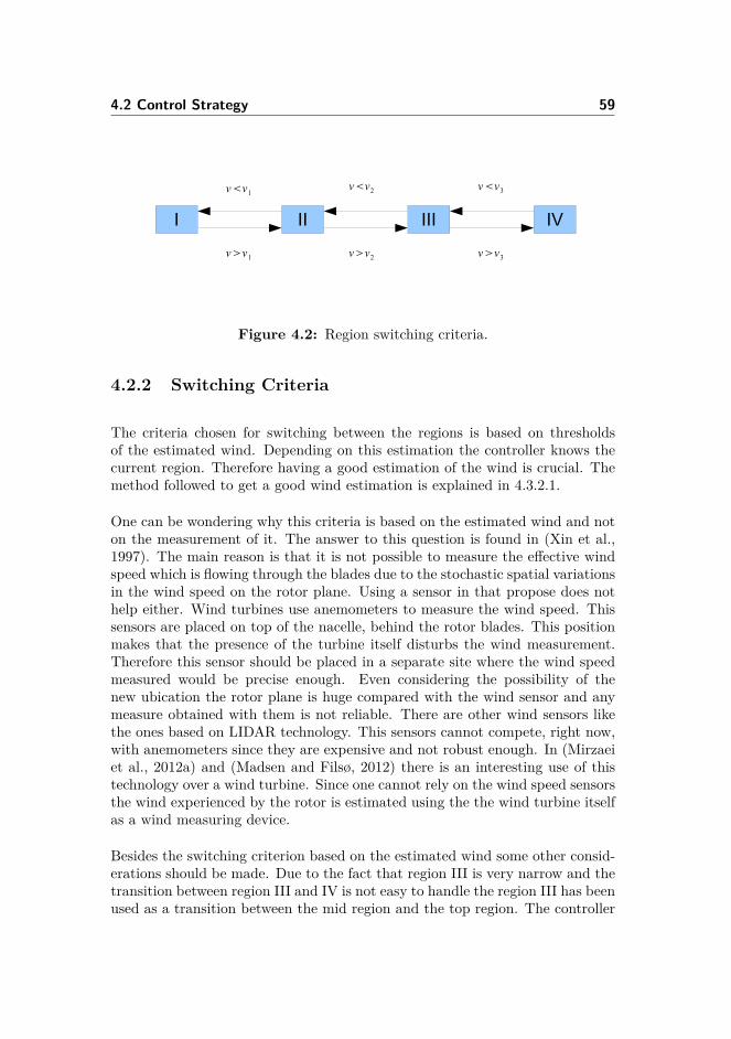
Figure 4.2: Region switching criteria.
4.2.2 Switching Criteria
The criteria chosen for switching between the regions is based on thresholdsof the estimated wind. Depending on this estimation the controller knows thecurrent region. Therefore having a good estimation of the wind is crucial. Themethod followed to get a good wind estimation is explained in 4.3.2.1.
One can be wondering why this criteria is based on the estimated wind and noton the measurement of it. The answer to this question is found in (Xin et al.,1997). The main reason is that it is not possible to measure the effective windspeed which is flowing through the blades due to the stochastic spatial variationsin the wind speed on the rotor plane. Using a sensor in that propose does nothelp either. Wind turbines use anemometers to measure the wind speed. Thissensors are placed on top of the nacelle, behind the rotor blades. This positionmakes that the presence of the turbine itself disturbs the wind measurement.Therefore this sensor should be placed in a separate site where the wind speedmeasured would be precise enough. Even considering the possibility of thenew ubication the rotor plane is huge compared with the wind sensor and anymeasure obtained with them is not reliable. There are other wind sensors likethe ones based on LIDAR technology. This sensors cannot compete, right now,with anemometers since they are expensive and not robust enough. In (Mirzaeiet al., 2012a) and (Madsen and Filsø, 2012) there is an interesting use of thistechnology over a wind turbine. Since one cannot rely on the wind speed sensorsthe wind experienced by the rotor is estimated using the the wind turbine itselfas a wind measuring device.
Besides the switching criterion based on the estimated wind some other consid-erations should be made. Due to the fact that region III is very narrow and thetransition between region III and IV is not easy to handle the region III has beenused as a transition between the mid region and the top region. The controller

60 Implementation and Results
has been tuned in order to achieve soft transitions between the regions.
4.2.3 Control Strategy Summary
Compared to other control problems the wind turbines dynamics are driven bya disturbance: the wind speed. Beside other variables, the wind speed is oneof the main variables to select the operating conditions of wind turbines, likeshown in section 2.3.
As it has already been mentioned in the previous section there are four differentoperation modes of a wind turbine and each of them has different characteristics.A good way of handling this variation in the operating conditions is using acontrol strategy like the gain scheduling.
In this project to regulate the inverted pendulum turbine, the technique usedis based on a gain scheduling LQG controller which is able to compensate thenon-linearities inherent in wind turbines.
When using gain scheduling technique some variables are used to decide thecurrent operating point. In the baseline controller explained in section 4.1 thepitch angle and the generator rotational speed are used as scheduling variables.In other studies like (Hammerum, 2006) the gain scheduling variables used arethe produced electrical power, the pitch and the generator rotational speed.
In this project the chosen schedule variable is the wind speed which has theadvantage that this variable by itself can be used over the entire operatingrange.
In order to have a good performance of the control action it is necessary tohave a precise and reliable value of the effective wind speed. Since there areno accurate measurements of the wind speed available using sensors the windneeds to be estimated. Because of that having a reliable estimation of the windis very important to have a good performance since the estimated wind speedis used to determine the operating point.
4.2 Control Strategy 61
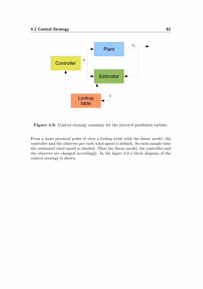
Figure 4.3: Control strategy summary for the inverted pendulum turbine.
From a more practical point of view a lookup table with the linear model, thecontroller and the observer per each wind speed is defined. So each sample timethe estimated wind speed is checked. Then the linear model, the controller andthe observer are changed accordingly. In the figure 4.3 a block diagram of thecontrol strategy is shown.
62 Implementation and Results
4.3 Control Implementation
4.3.1 Discrete Model
The mathematical model of the inverted pendulum turbine has been presentedin continuous time. Since all the simulations are done in discrete time the systemneeds to be discretized. The chosen sampling time is Ts = 0.05s, which give asampling frequency fs = 20Hz.
When modelling a wind turbine one of the components with faster time constantis the generator torque actuator. From (Henriksen, 2007) the time constant ofthis actuator is τ = 0.1s. Following the well-known sampling criteria of Nyquist,that can be found in (Proakis and Manolakis, 2007), the sampling time has beenchosen to be half of the fastest time constant
Ts = τ
2 = 0.05s (4.6)
In this thesis the model of the generator torque actuator is not used but thinkingon possible future changes it has been decided the sampling time of 0.05s.
The method used to discretise the system is the well-known zero order holding.This method has the peculiarity that in the sample points the discrete value andthe continuous one are equal, then the discrete value is kept constant until thenext sample point where both signals, the continuous and the discrete, are equalagain. This method has been used since is a proven method that on systemswith time constants larger than two times the sampling time, like the currentone, give good results.
4.3.2 Wind and States Estimation
4.3.2.1 Wind Estimation
In this project having a good estimation of the wind is really important sincedepending on that the control action applied to the system is different. In(Østergaard et al., 2007) there is an interesting approach of how to estimate thewind speed but the technique used in this project is extracted from (Xin et al.,1997) where a broad explanation can be found.
4.3 Control Implementation 63
To get a good estimation of the wind the model of the inverted pendulumturbine has been extended with two new states: the wind speed v and the windacceleration v.
Having the state space description of the inverted pendulum turbine
x = Ax+Bu+ Ev + dx (4.7)
y = Cx+Du+ dy (4.8)
and the state space description of the stochastic wind
[vtvt
]=[
0 1−1p1p2
−p1−p2p1p2
]︸ ︷︷ ︸
Aw
[vtvt
]+[
0k
p1p2
]e (4.9)
e ∈ N(0, 1) (4.10)
then the extended model is
xe = Aexe +Beue + dxe (4.11)ye = Cexe +Deue + dye (4.12)
where
Ae =[A[3x3] E[3x1] 0[3x1]0[2x3] Aw[2x2]
]Be =
[B[3x2]0[2x2]
]dxe =
[dx[3x1]0[2x1]
](4.13)
Ce =[C[3x3] 0[3x2]
]De =
[D[3x2]
]dye =
[dy[3x1]
](4.14)
xe =
x[3x1]v[1x1]v[1x1]
ye = y ue = u (4.15)

64 Implementation and Results
Notice that since it is not possible to control the wind the input matrix has beenextended with zeros.
The observability of the extended system have been check with the observabilitymatrix Mo defined in section 2.5.1.3. The rank of Mo is five for the whole windspeed range. That means that all the states of the extended model, including vand v, can be estimated observing the measurements.
In figures 4.4 to 4.6 the results of using this estimation technique can be seen. Infigure 4.4 the estimation of the wind is shown when into the system deterministicsteps on the wind are introduced and in figure 4.5 when the stochastic wind isintroduced. In figure 4.6 the error of estimation in the stochastic case is shown.
0 2 4 6 8 10 12 14 16 18 2014.5
15
15.5
16
16.5
17
17.5
Windspeed[m
/s]
Time [s] — Ts = 0.05s
Estimated windReal wind
Figure 4.4: Example of wind speed estimation: deterministic steps.
From the deterministic simulation it can be seen that the wind speed estimationis fast, it has a time constant of τ = 0.2s, and precise, the order of magnitudeof steady error of estimation is 0.001 m/s.
From the stochastic simulation it can be seen that the wind can be estimatedwith a good accuracy when having the stochastic wind. The mean value ofthe error of estimation is 0.0042 m/s and the standard deviation is 0.0485 m/s.The dynamics of the wind turbine change according to the wind. Having anestimation accuracy around 0.1 m/s can reflect all the dynamical changes of thewind turbine with precision. The results shown that the estimation of the windis not going to be a problem while controlling the system.
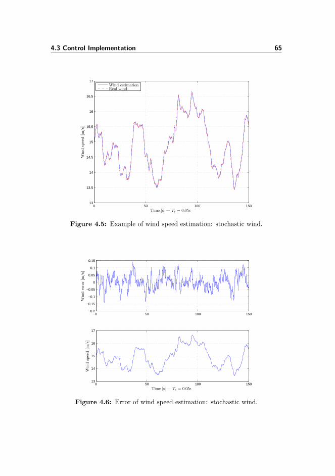
4.3 Control Implementation 65
0 50 100 15013
13.5
14
14.5
15
15.5
16
16.5
17
Time [s] — Ts = 0.05s
Windspeed[m
/s]
Wind estimationReal wind
Figure 4.5: Example of wind speed estimation: stochastic wind.
0 50 100 150−0.2
−0.15
−0.1
−0.05
0
0.05
0.1
0.15
Winderror[m
/s]
0 50 100 15013
14
15
16
17
Windspeed[m
/s]
Time [s] — Ts = 0.05s
Figure 4.6: Error of wind speed estimation: stochastic wind.
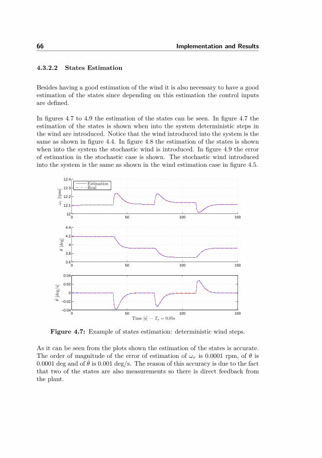
66 Implementation and Results
4.3.2.2 States Estimation
Besides having a good estimation of the wind it is also necessary to have a goodestimation of the states since depending on this estimation the control inputsare defined.
In figures 4.7 to 4.9 the estimation of the states can be seen. In figure 4.7 theestimation of the states is shown when into the system deterministic steps inthe wind are introduced. Notice that the wind introduced into the system is thesame as shown in figure 4.4. In figure 4.8 the estimation of the states is shownwhen into the system the stochastic wind is introduced. In figure 4.9 the errorof estimation in the stochastic case is shown. The stochastic wind introducedinto the system is the same as shown in the wind estimation case in figure 4.5.
0 50 100 15012
12.1
12.2
12.3
12.4
ωr[rpm]
EstimationReal
0 50 100 1503.6
3.8
4
4.2
4.4
θ[deg]
0 50 100 150−0.04
−0.02
0
0.02
0.04
Time [s] — Ts = 0.05s
θ[deg/s]
Figure 4.7: Example of states estimation: deterministic wind steps.
As it can be seen from the plots shown the estimation of the states is accurate.The order of magnitude of the error of estimation of ωr is 0.0001 rpm, of θ is0.0001 deg and of θ is 0.001 deg/s. The reason of this accuracy is due to the factthat two of the states are also measurements so there is direct feedback fromthe plant.
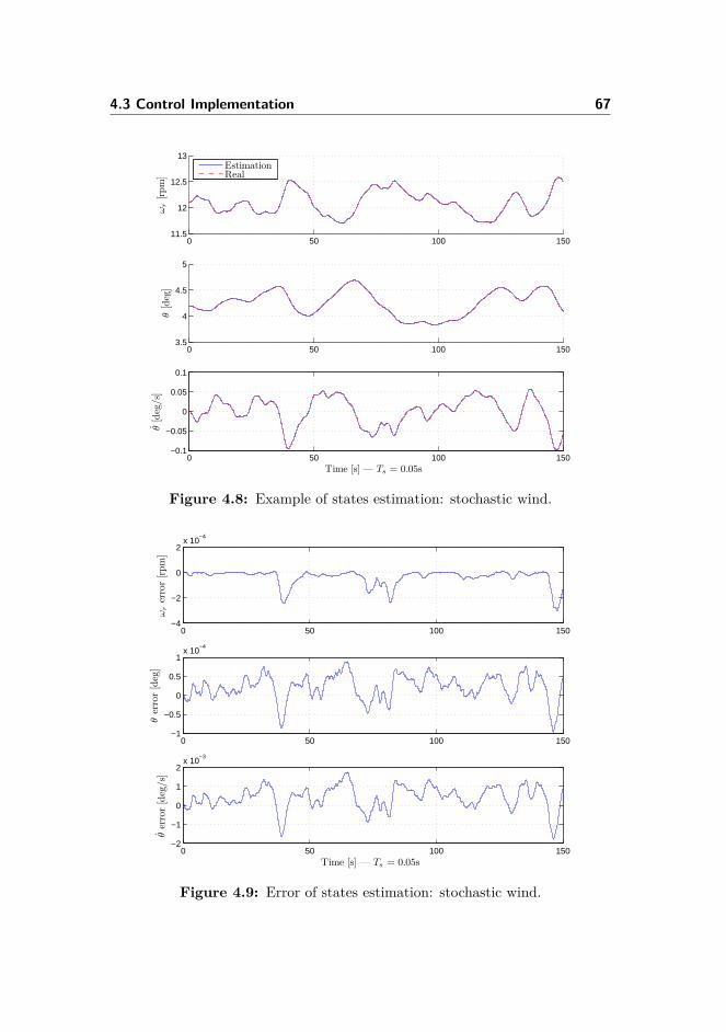
4.3 Control Implementation 67
0 50 100 15011.5
12
12.5
13ωr[rpm]
EstimationReal
0 50 100 1503.5
4
4.5
5
θ[deg]
0 50 100 150−0.1
−0.05
0
0.05
0.1
Time [s] — Ts = 0.05s
θ[deg/s]
Figure 4.8: Example of states estimation: stochastic wind.
0 50 100 150−4
−2
0
2x 10
−4
ωrerror[rpm]
0 50 100 150−1
−0.5
0
0.5
1x 10
−4
θerror[deg]
0 50 100 150−2
−1
0
1
2x 10
−3
Time [s] — Ts = 0.05s
θerror[deg/s]
Figure 4.9: Error of states estimation: stochastic wind.
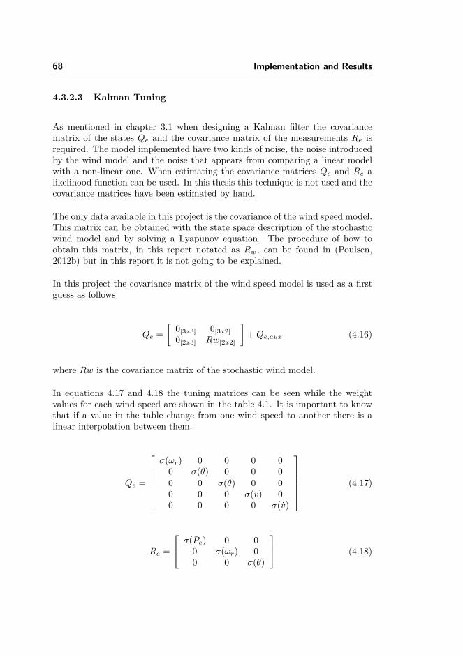
68 Implementation and Results
4.3.2.3 Kalman Tuning
As mentioned in chapter 3.1 when designing a Kalman filter the covariancematrix of the states Qe and the covariance matrix of the measurements Re isrequired. The model implemented have two kinds of noise, the noise introducedby the wind model and the noise that appears from comparing a linear modelwith a non-linear one. When estimating the covariance matrices Qe and Re alikelihood function can be used. In this thesis this technique is not used and thecovariance matrices have been estimated by hand.
The only data available in this project is the covariance of the wind speed model.This matrix can be obtained with the state space description of the stochasticwind model and by solving a Lyapunov equation. The procedure of how toobtain this matrix, in this report notated as Rw, can be found in (Poulsen,2012b) but in this report it is not going to be explained.
In this project the covariance matrix of the wind speed model is used as a firstguess as follows
Qe =[
0[3x3] 0[3x2]0[2x3] Rw[2x2]
]+Qe,aux (4.16)
where Rw is the covariance matrix of the stochastic wind model.
In equations 4.17 and 4.18 the tuning matrices can be seen while the weightvalues for each wind speed are shown in the table 4.1. It is important to knowthat if a value in the table change from one wind speed to another there is alinear interpolation between them.
Qe =
σ(ωr) 0 0 0 0
0 σ(θ) 0 0 00 0 σ(θ) 0 00 0 0 σ(v) 00 0 0 0 σ(v)
(4.17)
Re =
σ(Pe) 0 00 σ(ωr) 00 0 σ(θ)
(4.18)
4.3 Control Implementation 69
Table 4.1: Kalman Filter Weight Values.
v [m/s] σ(ωr) σ(θ) σ(θ) σ(v) σ(v) σ(Pe) σ(ωr) σ(θ)3 1e0 1e0 1e0 1e3 1e2 1e-4 1e-4 1e-3
10.5 1e0 1e0 1e0 1e3 1e2 1e-4 1e-4 1e-312 1e0 1e0 1e0 5e2 1e1 1e-4 1e-4 1e-315 5e1 1e0 1e0 5e4 1e3 1e-4 1e-4 1e-325 5e1 1e0 1e0 5e4 1e3 1e-4 1e-4 1e-3
Since the noise introduced by the difference between the linear model and thenon-linear one is higher than the noise introduced by the wind the v and vcomponent in Qe is higher than the components from Rw. As an exampleof how the weights have been obtained the way to get the weight θ in Re isexplained. Knowing that the maximum value of θ is 8.71 degrees and supposingthat the sensor used to measure this inclination can make errors around 5% themaximum error of measurement is the 5% of the 8.71 deg, then the covariancevalue of θ in Re could be estimated as
σ(θ) = 8.71 deg π rad
180 deg 5% = 7.6e− 3 rad ≈ 1e− 3 rad (4.19)
The other components have been tuned by hand in a similar way.
From a practical point of view a high weight on a component in the covariancematrix results as a high priority of having good estimation on that component.
4.3.3 Offset-Free Performance
Without implementing any offset-free method it is expected to have offset per-formance. In figure 4.10 there is the response when into the system, controlledby a LQG regulator, an step on the wind is introduced.
It can be seen that the control implemented have a small offset. In the electricalpower the offset is 0.2 % of the reference value and in the rotational speed is0.18 % of the reference value.
The two offset-free methods introduced in section 3.4 have been implemented.In the integral action case the integrator is placed in the rotational speed ωr. Ithas been proved that just with one integrator the zero offset performance canbe achieved for all the regions.
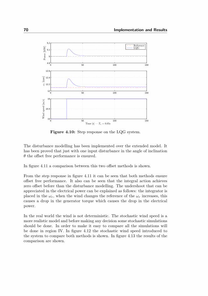
70 Implementation and Results
0 50 100 1504.9
5
5.1
5.2Pow
er[M
W] Reference
LQG
0 50 100 15012
12.2
12.4
12.6
ωr[rpm]
0 50 100 15015
15.5
16
Windspeed[m
/s]
Time [s] — Ts = 0.05s
Figure 4.10: Step response on the LQG system.
The disturbance modelling has been implemented over the extended model. Ithas been proved that just with one input disturbance in the angle of inclinationθ the offset free performance is ensured.
In figure 4.11 a comparison between this two offset methods is shown.
From the step response in figure 4.11 it can be seen that both methods ensureoffset free performance. It also can be seen that the integral action achieveszero offset before than the disturbance modelling. The undershoot that can beappreciated in the electrical power can be explained as follows: the integrator isplaced in the ωr, when the wind changes the reference of the ωr increases, thiscauses a drop in the generator torque which causes the drop in the electricalpower.
In the real world the wind is not deterministic. The stochastic wind speed is amore realistic model and before making any decision some stochastic simulationsshould be done. In order to make it easy to compare all the simulations willbe done in region IV. In figure 4.12 the stochastic wind speed introduced tothe system to compare both methods is shown. In figure 4.13 the results of thecomparison are shown.
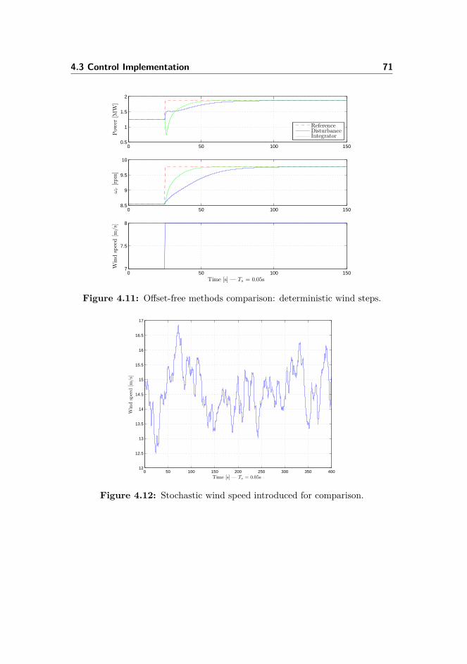
4.3 Control Implementation 71
0 50 100 1500.5
1
1.5
2
Pow
er[M
W]
ReferenceDisturbanceIntegrator
0 50 100 1508.5
9
9.5
10
ωr[rpm]
0 50 100 1507
7.5
8
Windspeed[m
/s]
Time [s] — Ts = 0.05s
Figure 4.11: Offset-free methods comparison: deterministic wind steps.
0 50 100 150 200 250 300 350 40012
12.5
13
13.5
14
14.5
15
15.5
16
16.5
17
Windspeed[m
/s]
Time [s] — Ts = 0.05s
Figure 4.12: Stochastic wind speed introduced for comparison.
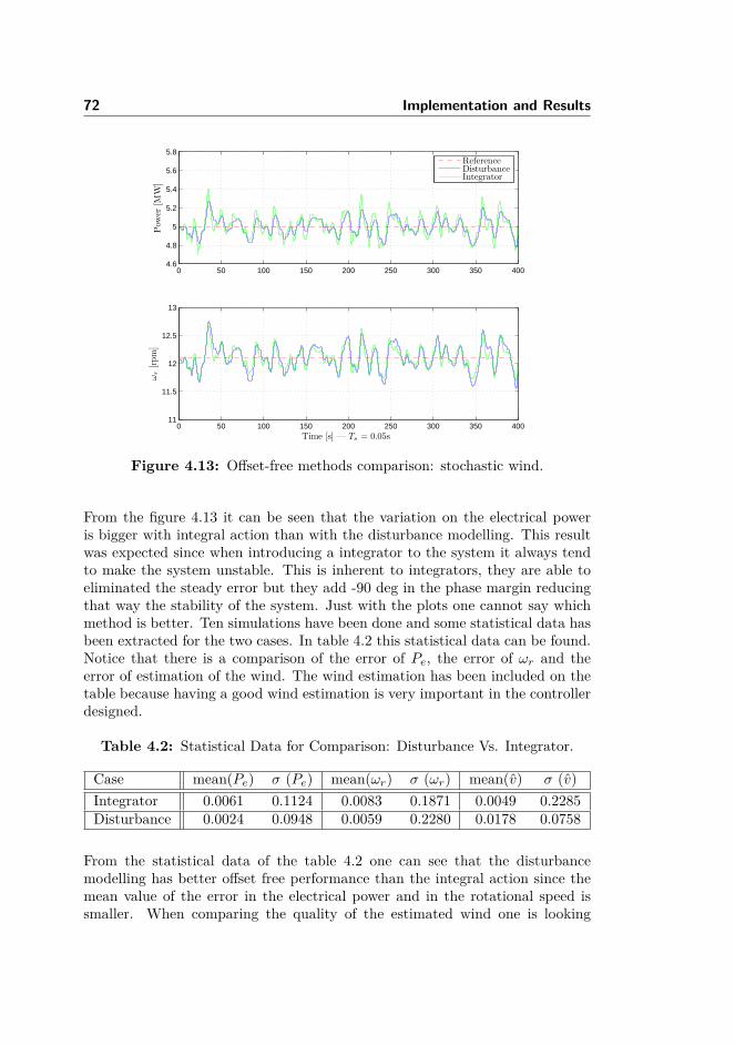
72 Implementation and Results
0 50 100 150 200 250 300 350 4004.6
4.8
5
5.2
5.4
5.6
5.8Pow
er[M
W]
ReferenceDisturbanceIntegrator
0 50 100 150 200 250 300 350 40011
11.5
12
12.5
13
ωr[rpm]
Time [s] — Ts = 0.05s
Figure 4.13: Offset-free methods comparison: stochastic wind.
From the figure 4.13 it can be seen that the variation on the electrical poweris bigger with integral action than with the disturbance modelling. This resultwas expected since when introducing a integrator to the system it always tendto make the system unstable. This is inherent to integrators, they are able toeliminated the steady error but they add -90 deg in the phase margin reducingthat way the stability of the system. Just with the plots one cannot say whichmethod is better. Ten simulations have been done and some statistical data hasbeen extracted for the two cases. In table 4.2 this statistical data can be found.Notice that there is a comparison of the error of Pe, the error of ωr and theerror of estimation of the wind. The wind estimation has been included on thetable because having a good wind estimation is very important in the controllerdesigned.
Table 4.2: Statistical Data for Comparison: Disturbance Vs. Integrator.
Case mean(Pe) σ (Pe) mean(ωr) σ (ωr) mean(v) σ (v)Integrator 0.0061 0.1124 0.0083 0.1871 0.0049 0.2285Disturbance 0.0024 0.0948 0.0059 0.2280 0.0178 0.0758
From the statistical data of the table 4.2 one can see that the disturbancemodelling has better offset free performance than the integral action since themean value of the error in the electrical power and in the rotational speed issmaller. When comparing the quality of the estimated wind one is looking
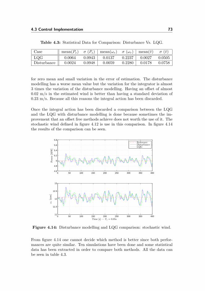
4.3 Control Implementation 73
Table 4.3: Statistical Data for Comparison: Disturbance Vs. LQG.
Case mean(Pe) σ (Pe) mean(ωr) σ (ωr) mean(v) σ (v)LQG 0.0064 0.0943 0.0137 0.2237 0.0027 0.0505Disturbance 0.0024 0.0948 0.0059 0.2280 0.0178 0.0758
for zero mean and small variation in the error of estimation. The disturbancemodelling has a worse mean value but the variation for the integrator is almost3 times the variation of the disturbance modelling. Having an offset of almost0.02 m/s in the estimated wind is better than having a standard deviation of0.23 m/s. Because all this reasons the integral action has been discarded.
Once the integral action has been discarded a comparison between the LQGand the LQG with disturbance modelling is done because sometimes the im-provement that an offset free methods achieve does not worth the use of it. Thestochastic wind defined in figure 4.12 is use in this comparison. In figure 4.14the results of the comparison can be seen.
0 50 100 150 200 250 300 350 4004.6
4.8
5
5.2
5.4
5.6
5.8
Pow
er[M
W]
ReferenceDisturbanceLQG
0 50 100 150 200 250 300 350 40011
11.5
12
12.5
13
ωr[rpm]
Time [s] — Ts = 0.05s
Figure 4.14: Disturbance modelling and LQG comparison: stochastic wind.
From figure 4.14 one cannot decide which method is better since both perfor-mances are quite similar. Ten simulations have been done and some statisticaldata has been extracted in order to compare both methods. All the data canbe seen in table 4.3.
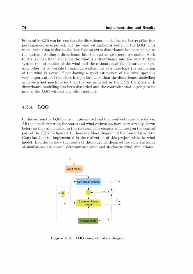
74 Implementation and Results
From table 4.3 it can be seen that the disturbance modelling has better offset freeperformance, as expected, but the wind estimation is better in the LQG. Thisworse estimation is due to the fact that an extra disturbance has been added tothe system. Adding a disturbance into the system give more estimation workto the Kalman filter and since the wind is a disturbance into the wind turbinesystem the estimation of the wind and the estimation of the disturbance fighteach other. It is possible to reach zero offset but as a drawback the estimationof the wind is worse. Since having a good estimation of the wind speed isvery important and the offset free performance than the disturbance modellingachieves is not much better than the one achieved by the LQG the LQG withdisturbance modelling has been discarded and the controller that is going to beused is the LQG without any offset method.
4.3.4 LQG
In this section the LQG control implemented and the results obtained are shown.All the details referring the states and wind estimation have been already shownbefore so they are omitted in this section. This chapter is focused on the controlpart of the LQG. In figure 4.15 there is a block diagram of the Linear QuadraticGaussian Control implemented in the realization of this project with the windmodel. In order to show the results of the controller designed two different kindsof simulations are shown: deterministic wind and stochastic wind simulations.
Figure 4.15: LQG complete block diagram.
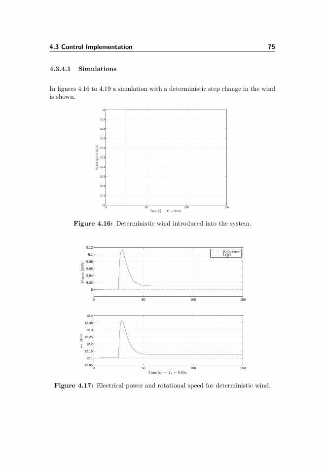
4.3 Control Implementation 75
4.3.4.1 Simulations
In figures 4.16 to 4.19 a simulation with a deterministic step change in the windis shown.
0 50 100 15015
15.1
15.2
15.3
15.4
15.5
15.6
15.7
15.8
15.9
16
Windspeed[m
/s]
Time [s] — Ts = 0.05s
Figure 4.16: Deterministic wind introduced into the system.
0 50 100 150
5
5.02
5.04
5.06
5.08
5.1
5.12
Pow
er[M
W]
ReferenceLQG
0 50 100 15012.05
12.1
12.15
12.2
12.25
12.3
12.35
12.4
ωr[rpm]
Time [s] — Ts = 0.05s
Figure 4.17: Electrical power and rotational speed for deterministic wind.
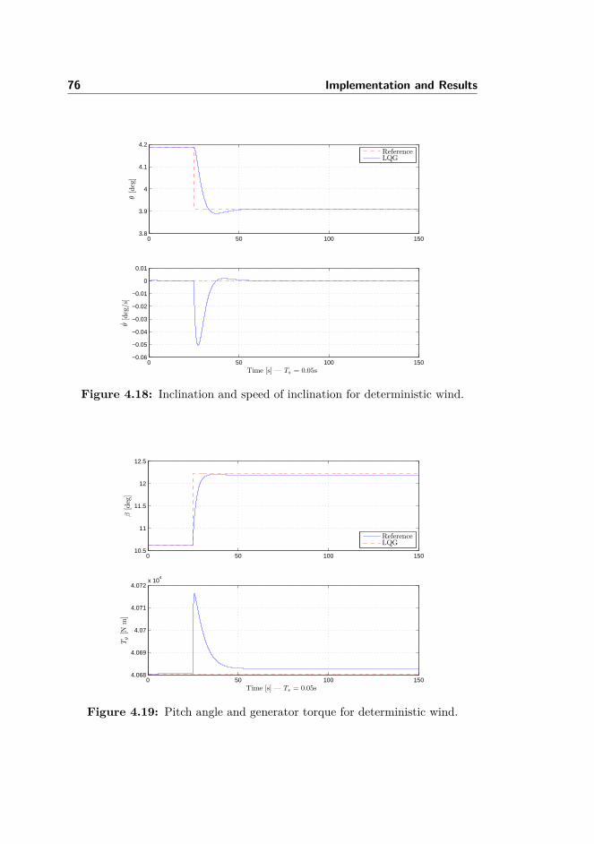
76 Implementation and Results
0 50 100 1503.8
3.9
4
4.1
4.2
θ[deg]
ReferenceLQG
0 50 100 150−0.06
−0.05
−0.04
−0.03
−0.02
−0.01
0
0.01
θ[deg/s]
Time [s] — Ts = 0.05s
Figure 4.18: Inclination and speed of inclination for deterministic wind.
0 50 100 15010.5
11
11.5
12
12.5
β[deg]
ReferenceLQG
0 50 100 1504.068
4.069
4.07
4.071
4.072x 10
4
Tg[N
m]
Time [s] — Ts = 0.05s
Figure 4.19: Pitch angle and generator torque for deterministic wind.
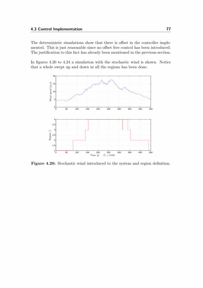
4.3 Control Implementation 77
The deterministic simulations show that there is offset in the controller imple-mented. This is just reasonable since no offset free control has been introduced.The justification to this fact has already been mentioned in the previous section.
In figures 4.20 to 4.24 a simulation with the stochastic wind is shown. Noticethat a whole swept up and down in all the regions has been done.
0 50 100 150 200 250 300 350 400 4500
5
10
15
20
Windspeed[m
/s]
0 50 100 150 200 250 300 350 400 4501
1.5
2
2.5
3
3.5
4
Region[-]
Time [s] — Ts = 0.05s
Figure 4.20: Stochastic wind introduced to the system and region definition.
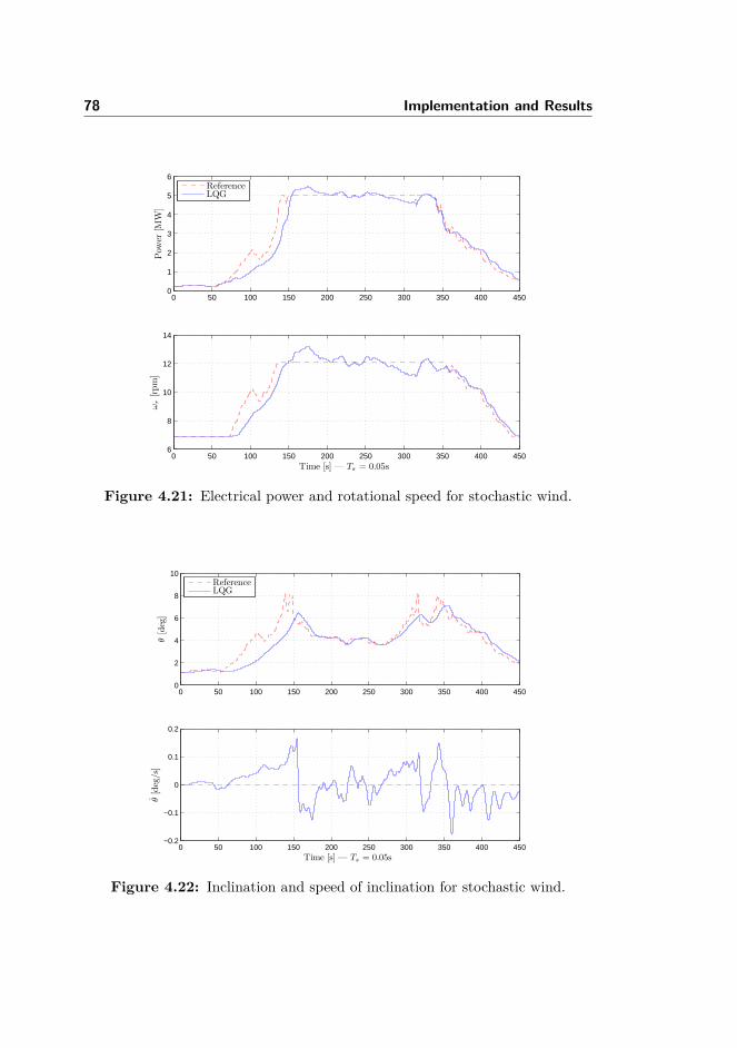
78 Implementation and Results
0 50 100 150 200 250 300 350 400 4500
1
2
3
4
5
6
Pow
er[M
W]
ReferenceLQG
0 50 100 150 200 250 300 350 400 4506
8
10
12
14
ωr[rpm]
Time [s] — Ts = 0.05s
Figure 4.21: Electrical power and rotational speed for stochastic wind.
0 50 100 150 200 250 300 350 400 4500
2
4
6
8
10
θ[deg]
ReferenceLQG
0 50 100 150 200 250 300 350 400 450−0.2
−0.1
0
0.1
0.2
θ[deg/s]
Time [s] — Ts = 0.05s
Figure 4.22: Inclination and speed of inclination for stochastic wind.
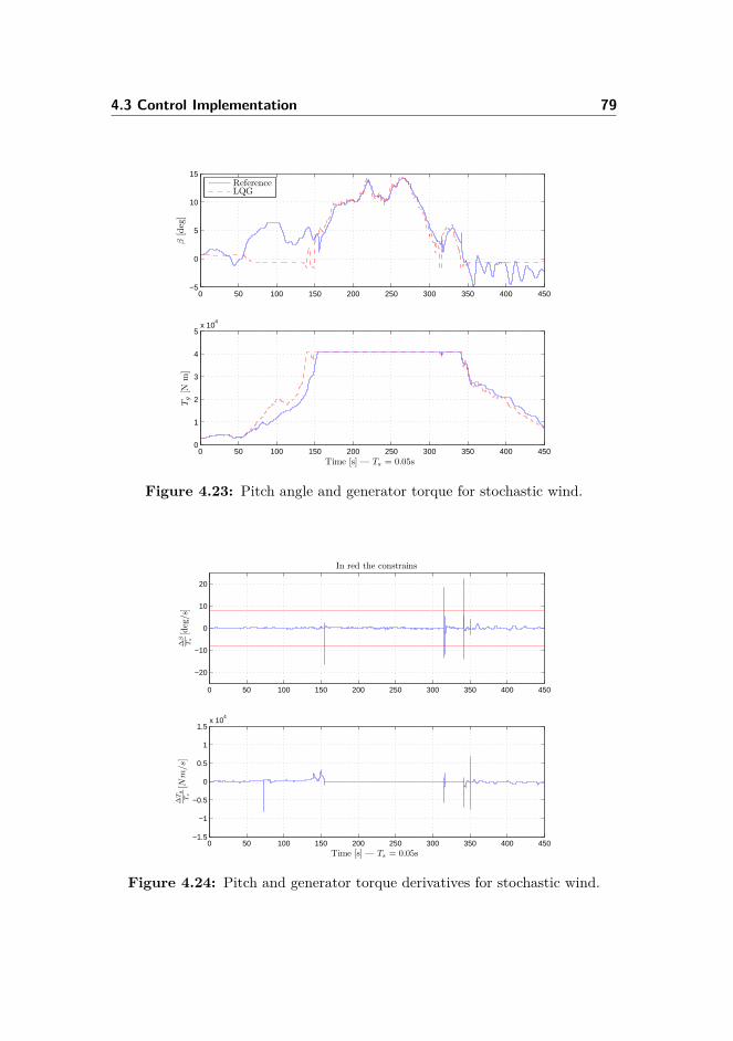
4.3 Control Implementation 79
0 50 100 150 200 250 300 350 400 450−5
0
5
10
15β[deg]
ReferenceLQG
0 50 100 150 200 250 300 350 400 4500
1
2
3
4
5x 10
4
Tg[N
m]
Time [s] — Ts = 0.05s
Figure 4.23: Pitch angle and generator torque for stochastic wind.
0 50 100 150 200 250 300 350 400 450
−20
−10
0
10
20
In red the constrains
∆β
Ts[deg/s]
0 50 100 150 200 250 300 350 400 450−1.5
−1
−0.5
0
0.5
1
1.5x 10
4
∆Tg
Ts[N
m/s]
Time [s] — Ts = 0.05s
Figure 4.24: Pitch and generator torque derivatives for stochastic wind.
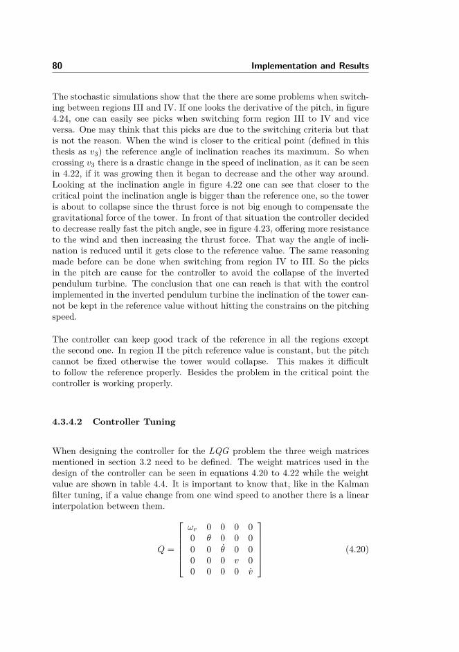
80 Implementation and Results
The stochastic simulations show that the there are some problems when switch-ing between regions III and IV. If one looks the derivative of the pitch, in figure4.24, one can easily see picks when switching form region III to IV and viceversa. One may think that this picks are due to the switching criteria but thatis not the reason. When the wind is closer to the critical point (defined in thisthesis as v3) the reference angle of inclination reaches its maximum. So whencrossing v3 there is a drastic change in the speed of inclination, as it can be seenin 4.22, if it was growing then it began to decrease and the other way around.Looking at the inclination angle in figure 4.22 one can see that closer to thecritical point the inclination angle is bigger than the reference one, so the toweris about to collapse since the thrust force is not big enough to compensate thegravitational force of the tower. In front of that situation the controller decidedto decrease really fast the pitch angle, see in figure 4.23, offering more resistanceto the wind and then increasing the thrust force. That way the angle of incli-nation is reduced until it gets close to the reference value. The same reasoningmade before can be done when switching from region IV to III. So the picksin the pitch are cause for the controller to avoid the collapse of the invertedpendulum turbine. The conclusion that one can reach is that with the controlimplemented in the inverted pendulum turbine the inclination of the tower can-not be kept in the reference value without hitting the constrains on the pitchingspeed.
The controller can keep good track of the reference in all the regions exceptthe second one. In region II the pitch reference value is constant, but the pitchcannot be fixed otherwise the tower would collapse. This makes it difficultto follow the reference properly. Besides the problem in the critical point thecontroller is working properly.
4.3.4.2 Controller Tuning
When designing the controller for the LQG problem the three weigh matricesmentioned in section 3.2 need to be defined. The weight matrices used in thedesign of the controller can be seen in equations 4.20 to 4.22 while the weightvalue are shown in table 4.4. It is important to know that, like in the Kalmanfilter tuning, if a value change from one wind speed to another there is a linearinterpolation between them.
Q =
ωr 0 0 0 00 θ 0 0 00 0 θ 0 00 0 0 v 00 0 0 0 v
(4.20)
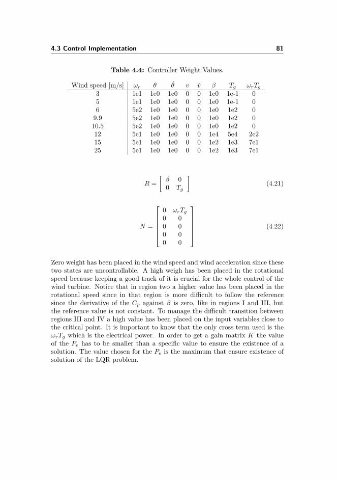
4.3 Control Implementation 81
Table 4.4: Controller Weight Values.
Wind speed [m/s] ωr θ θ v v β Tg ωrTg3 1e1 1e0 1e0 0 0 1e0 1e-1 05 1e1 1e0 1e0 0 0 1e0 1e-1 06 5e2 1e0 1e0 0 0 1e0 1e2 09.9 5e2 1e0 1e0 0 0 1e0 1e2 010.5 5e2 1e0 1e0 0 0 1e0 1e2 012 5e1 1e0 1e0 0 0 1e4 5e4 2e215 5e1 1e0 1e0 0 0 1e2 1e3 7e125 5e1 1e0 1e0 0 0 1e2 1e3 7e1
R =[β 00 Tg
](4.21)
N =
0 ωrTg0 00 00 00 0
(4.22)
Zero weight has been placed in the wind speed and wind acceleration since thesetwo states are uncontrollable. A high weigh has been placed in the rotationalspeed because keeping a good track of it is crucial for the whole control of thewind turbine. Notice that in region two a higher value has been placed in therotational speed since in that region is more difficult to follow the referencesince the derivative of the Cp against β is zero, like in regions I and III, butthe reference value is not constant. To manage the difficult transition betweenregions III and IV a high value has been placed on the input variables close tothe critical point. It is important to know that the only cross term used is theωrTg which is the electrical power. In order to get a gain matrix K the valueof the Pe has to be smaller than a specific value to ensure the existence of asolution. The value chosen for the Pe is the maximum that ensure existence ofsolution of the LQR problem.
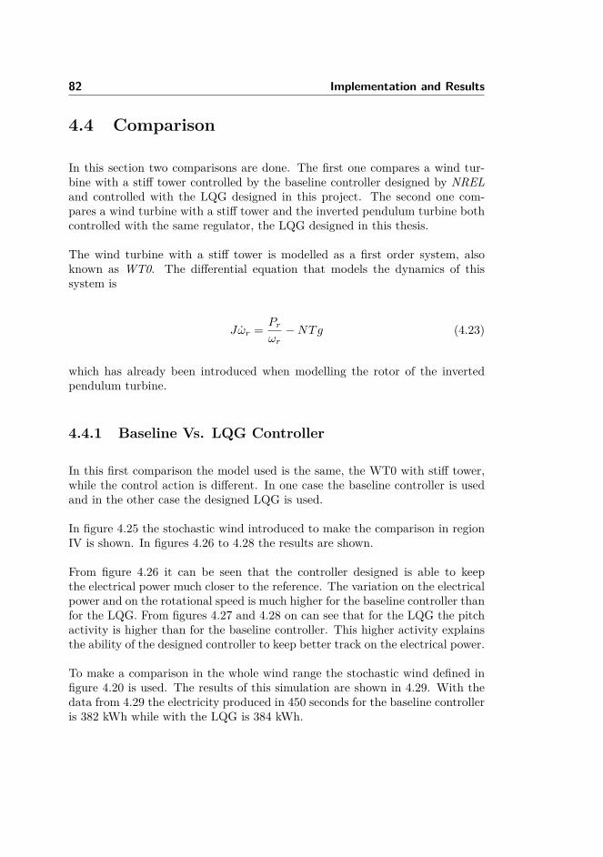
82 Implementation and Results
4.4 Comparison
In this section two comparisons are done. The first one compares a wind tur-bine with a stiff tower controlled by the baseline controller designed by NRELand controlled with the LQG designed in this project. The second one com-pares a wind turbine with a stiff tower and the inverted pendulum turbine bothcontrolled with the same regulator, the LQG designed in this thesis.
The wind turbine with a stiff tower is modelled as a first order system, alsoknown as WT0. The differential equation that models the dynamics of thissystem is
Jωr = Prωr−NTg (4.23)
which has already been introduced when modelling the rotor of the invertedpendulum turbine.
4.4.1 Baseline Vs. LQG Controller
In this first comparison the model used is the same, the WT0 with stiff tower,while the control action is different. In one case the baseline controller is usedand in the other case the designed LQG is used.
In figure 4.25 the stochastic wind introduced to make the comparison in regionIV is shown. In figures 4.26 to 4.28 the results are shown.
From figure 4.26 it can be seen that the controller designed is able to keepthe electrical power much closer to the reference. The variation on the electricalpower and on the rotational speed is much higher for the baseline controller thanfor the LQG. From figures 4.27 and 4.28 on can see that for the LQG the pitchactivity is higher than for the baseline controller. This higher activity explainsthe ability of the designed controller to keep better track on the electrical power.
To make a comparison in the whole wind range the stochastic wind defined infigure 4.20 is used. The results of this simulation are shown in 4.29. With thedata from 4.29 the electricity produced in 450 seconds for the baseline controlleris 382 kWh while with the LQG is 384 kWh.
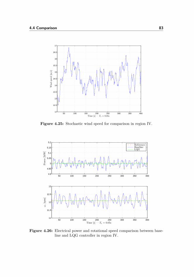
4.4 Comparison 83
50 100 150 200 250 300 350 40012
12.5
13
13.5
14
14.5
15
15.5
16
16.5
17
Windspeed[m
/s]
Time [s] — Ts = 0.05s
Figure 4.25: Stochastic wind speed for comparison in region IV.
50 100 150 200 250 300 350 4004.9
4.95
5
5.05
5.1
5.15
5.2
Pow
er[M
W]
ReferenceBaselineLQG
50 100 150 200 250 300 350 40011
11.5
12
12.5
13
ωr[rpm]
Time [s] — Ts = 0.05s
Figure 4.26: Electrical power and rotational speed comparison between base-line and LQG controller in region IV.
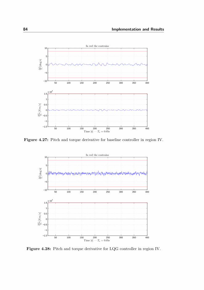
84 Implementation and Results
50 100 150 200 250 300 350 400−10
−5
0
5
10In red the contrains
∆β
Ts[deg/s]
50 100 150 200 250 300 350 400−1.5
−1
−0.5
0
0.5
1
1.5x 10
4
∆Tg
Ts[N
m/s
]
Time [s] — Ts = 0.05s
Figure 4.27: Pitch and torque derivative for baseline controller in region IV.
50 100 150 200 250 300 350 400−10
−5
0
5
10In red the contrains
∆β
Ts[deg/s]
50 100 150 200 250 300 350 400−1.5
−1
−0.5
0
0.5
1
1.5x 10
4
∆Tg
Ts[N
m/s
]
Time [s] — Ts = 0.05s
Figure 4.28: Pitch and torque derivative for LQG controller in region IV.
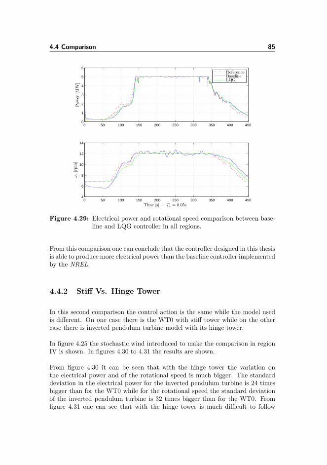
4.4 Comparison 85
0 50 100 150 200 250 300 350 400 4500
1
2
3
4
5
6
Pow
er[M
W]
ReferenceBaselineLQG
0 50 100 150 200 250 300 350 400 4504
6
8
10
12
14
ωr[rpm]
Time [s] — Ts = 0.05s
Figure 4.29: Electrical power and rotational speed comparison between base-line and LQG controller in all regions.
From this comparison one can conclude that the controller designed in this thesisis able to produce more electrical power than the baseline controller implementedby the NREL.
4.4.2 Stiff Vs. Hinge Tower
In this second comparison the control action is the same while the model usedis different. On one case there is the WT0 with stiff tower while on the othercase there is inverted pendulum turbine model with its hinge tower.
In figure 4.25 the stochastic wind introduced to make the comparison in regionIV is shown. In figures 4.30 to 4.31 the results are shown.
From figure 4.30 it can be seen that with the hinge tower the variation onthe electrical power and of the rotational speed is much bigger. The standarddeviation in the electrical power for the inverted pendulum turbine is 24 timesbigger than for the WT0 while for the rotational speed the standard deviationof the inverted pendulum turbine is 32 times bigger than for the WT0. Fromfigure 4.31 one can see that with the hinge tower is much difficult to follow
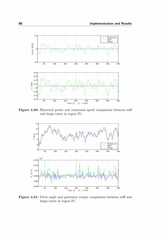
86 Implementation and Results
50 100 150 200 250 300 350 4004.5
5
5.5
Pow
er[M
W]
ReferenceStiffHinge
50 100 150 200 250 300 350 40011.4
11.6
11.8
12
12.2
12.4
12.6
12.8
ωr[rpm]
Time [s] — Ts = 0.05s
Figure 4.30: Electrical power and rotational speed comparison between stiffand hinge tower in region IV.
50 100 150 200 250 300 350 4004
6
8
10
12
14
β[deg]
ReferenceStiffHinge
50 100 150 200 250 300 350 4004.064
4.066
4.068
4.07
4.072
4.074x 10
4
Tg[N
m]
Time [s] — Ts = 0.05s
Figure 4.31: Pitch angle and generator torque comparison between stiff andhinge tower in region IV.
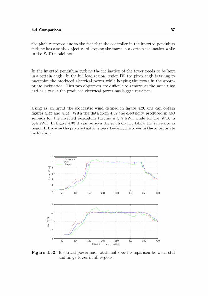
4.4 Comparison 87
the pitch reference due to the fact that the controller in the inverted pendulumturbine has also the objective of keeping the tower in a certain inclination whilein the WT0 model not.
In the inverted pendulum turbine the inclination of the tower needs to be keptin a certain angle. In the full load region, region IV, the pitch angle is trying tomaximize the produced electrical power while keeping the tower in the appro-priate inclination. This two objectives are difficult to achieve at the same timeand as a result the produced electrical power has bigger variation.
Using as an input the stochastic wind defined in figure 4.20 one can obtainfigures 4.32 and 4.33. With the data from 4.32 the electricity produced in 450seconds for the inverted pendulum turbine is 372 kWh while for the WT0 is384 kWh. In figure 4.33 it can be seen the pitch do not follow the reference inregion II because the pitch actuator is busy keeping the tower in the appropriateinclination.
50 100 150 200 250 300 350 4000
1
2
3
4
5
6
Pow
er[M
W]
ReferenceStiffHinge
50 100 150 200 250 300 350 4006
8
10
12
14
ωr[rpm]
Time [s] — Ts = 0.05s
Figure 4.32: Electrical power and rotational speed comparison between stiffand hinge tower in all regions.
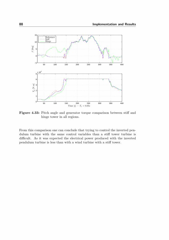
88 Implementation and Results
50 100 150 200 250 300 350 400−5
0
5
10
15
β[deg]
ReferenceStiffHinge
50 100 150 200 250 300 350 4000
1
2
3
4
5x 10
4
Tg[N
m]
Time [s] — Ts = 0.05s
Figure 4.33: Pitch angle and generator torque comparison between stiff andhinge tower in all regions.
From this comparison one can conclude that trying to control the inverted pen-dulum turbine with the same control variables than a stiff tower turbine isdifficult. As it was expected the electrical power produced with the invertedpendulum turbine is less than with a wind turbine with a stiff tower.

Chapter 5
Conclusions and Perspectives
In this chapter the conclusions of this project and the future perspectives of theinverted pendulum turbine are shown.
5.1 Conclusions
The main objective of this thesis is to study the feasibility of the inverted pen-dulum turbine. To reach this goal many sub-objectives have been achieved.
A model of the inverted pendulum turbine has been developed. The modelconsidered is composed by a 2-order system of the hinge tower and a 1-ordersystem of the rotor. The steady operation points for the inverted pendulumturbine have been obtained with the objective of maximizing the produced elec-trical power and keeping the hinge tower still. It has been shown that the steadystate points of a stiff tower wind turbine and of a hinge tower wind turbine arethe same but adding to the hinge tower the proper inclination angle. The non-linear model of the inverted pendulum turbine has been linearized at the steadyoperating points. The linear model obtained has been successfully comparedwith the non-linear one.
90 Conclusions and Perspectives
The model of the inverted pendulum turbine has been proved to be an unstablesystem, as it was expected. Using the same control inputs as current windturbines, pitch angle β and generator torque Tg, it has been proved that thesystem is controllable. Having the measurements of the electrical power, therotational speed and the angle of inclination is enough to be able to estimationof the states. All this measurements can easily be obtained with a proper sensor.
Once the model of the inverted pendulum turbine has been obtained and it hasbeen proved that it can be controlled and observed the next step is designingthe controller. It has been decided to use an optimal controller like the LinearQuadratic Regulator, which ensure a good performance, combined with an op-timal estimator based on a Kalman filter. This technique is known as LinearQuadratic Gaussian Control and it has been introduced and used in this project.In order to get offset free control some methods like Disturbance Modelling andIntegral Action have been studied.
The steady operation points of the inverted pendulum turbine define four dif-ferent regions in the wind speed range, each one with different properties. Ineach region the controller designed has been tuned differently according to thecontrol objective of the region. The region switching criteria used is based onthe estimated wind. To get the wind estimation the inverted pendulum turbinemodel has been extended and a Kalman filter has been used. The final controllerused in this project is a gain scheduling LQG controller based on the estimatedwind.
Form the simulations it has been shown that the method used to estimate thewind is reliable. It has also been shown that the offset-free methods implementeddo not provide such a good performance as it was expected. This could beexplained for the undesirable effect of adding integrators to an unstable system.The controller implemented has been proved to have good performance in allthe operation regions. It also has been shown that in the transition betweenregions III and IV there is an issue on keeping the pitch actuator constrainswhile trying to keep the tower in a proper inclination, this would need to beinvestigated.
The controller of the inverted pendulum turbine has been implemented on astiff tower wind turbine and it has been compared with the baseline controllerdesigned by theNREL. It has been shown that the regulator designed in thisthesis is able to produce more electrical power than the designed by the NREL.
The performance of the inverted pendulum turbine has been compared with astiff tower wind turbine regulated by the controller design in this thesis. It hasbeen shown that the variation of the electrical power for the hinge turbine ishigher than for the stiff tower turbine. This variation could be damped by the

5.1 Conclusions 91
wind park and at the point of connection with the grid the oscillations would bemuch lower. As it was expected the produced electrical power for the invertedpendulum turbine is lower than for the stiff tower wind turbine.
With all the things mentioned above now one can discuss the feasibility of theinverted pendulum turbine. It has been shown that the inverted pendulumturbine can be controlled with the pitch and the generator torque with the issuealready mention in the transition III to IV which should be investigated. It hasalso been shown that from a control point of view the mass of the tower couldbe reduced having as a result a lighter and cheaper structure. From (Fingershet al., 2006) the relation between the mass of the tower and its price is linear.Then from a control point of view the price of the tower could be reducedin a 20% having almost the same control problem, almost the same angle ofinclination (4% bigger), while the produced electrical power would be slightlylower, according to figure 4.32 about 0.5% less. Then, from a control point ofview and with deeper research on the issues mentioned, the inverted pendulumturbine is feasible. It is clear that the inverted pendulum turbine have newchallenging problem to overcome, but the arising challenges from this designcould be compensated by the benefit harvested.

92 Conclusions and Perspectives
5.2 Perspectives
This project is a first step on the investigation of the inverted pendulum turbineand it opens a wide range of possible future investigations and improvements.
On the modelling side of the project it would be very interesting to includeadditional effects and degrees of freedom to the model. Taking in account thatthe tower is moving forwards and backwards it would be interesting to modelthe relative wind speed over the rotor area. This consideration would lead toa stronger couple between the two sub-models implemented in this thesis: therotor and the hinge turbine. Having a model which is able to evaluate thefatigue loads over the components of the wind turbine, for example the tower,would be really attractive from a mechanical point of view since the stress ofthe components could be analysed and minimized. Moreover, it would also berecommended to include the flexibility of the drive-train. This considerationleads to a dynamic angular displacement between the angle of the generatorand the angle of the rotor. Adding models of the pitch and the torque actuatorswould make the model of the inverted pendulum wind turbine more realistic.Besides all this improvements, it would be very interesting to include the effectof the yaw angle and the angle of inclination of the wind turbine, omitted inthis project, with all the mechanical consequences derived from that.
Regarding the control part of the project there are some future implementationsthat would be very interesting to develop. First of all designing a controllerwhich objectives, besides maximizing produced electrical power and keeping thetower still, would be minimizing the stress of the components. That would bea very interesting approach since as a consequence the cost of this componentscould be reduced. The regulator designed in this thesis is able to control theinverted pendulum turbine when it is running but non start-up and stop tech-niques have been implemented. This techniques should be investigated to bringthe inverted pendulum turbine from a safety looked position to a running oneand vice versa. Researching in this methods is crucial for a possible future ap-plication of this uncommon wind turbine. Another interesting research wouldbe to study the possible existence of harmonic disturbances introduced in theelectrical power by the controller.
The control problem solved in this thesis can be extrapolated in the offshore case.The hinge effect in the offshore case could be achieved with a floating foundationcontrolled by some kind of mechanical actuator. This approach would allow toplace offshore wind farms in deep waters, where the quality of the wind is betterfor power extraction. As the reader can see the inverted pendulum turbine opena wide range of possibilities that in a close future could improve the wind energyworld and as a direct consequence the world energy system.
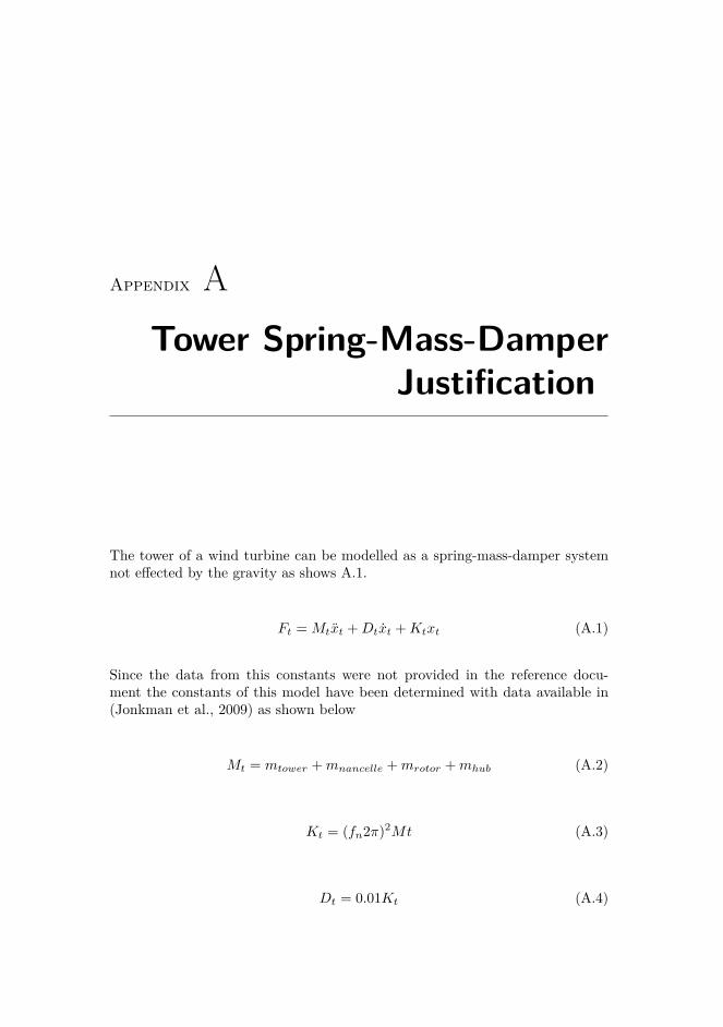
Appendix ATower Spring-Mass-Damper
Justification
The tower of a wind turbine can be modelled as a spring-mass-damper systemnot effected by the gravity as shows A.1.
Ft = Mtxt +Dtxt +Ktxt (A.1)
Since the data from this constants were not provided in the reference docu-ment the constants of this model have been determined with data available in(Jonkman et al., 2009) as shown below
Mt = mtower +mnancelle +mrotor +mhub (A.2)
Kt = (fn2π)2Mt (A.3)
Dt = 0.01Kt (A.4)

94 Tower Spring-Mass-Damper Justification
The equation A.3 comes from basics physics, where fn is the natural frequencyin Hz. The equation A.4 is a rule of thumb.
Since this project is working in angle of inclination instead of displacement allthe constants have been changed accordingly.

Appendix B
System Parameters
In this appendix all the data used in the simulations is displayed. There are twoconsideration to be made about table B.2:
• The total inertia of the generator and the rotor, J , is expressed withrespect to the low shaft.
• The spring Kt and damping constants Dt of the tower are the ones ob-tained in the appendix A.
Table B.1: Physical Constants.
Parameter Symbol used Value Units
Air density ρa 1.2041 kg/m3
Gravity g 9.81 m/s2
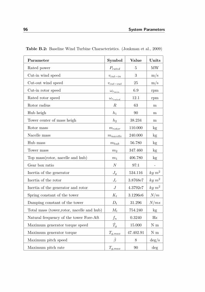
96 System Parameters
Table B.2: Baseline Wind Turbine Characteristics. (Jonkman et al., 2009)
Parameter Symbol Value Units
Rated power Prated 5 MW
Cut-in wind speed vcut−in 3 m/s
Cut-out wind speed vcut−out 25 m/s
Cut-in rotor speed ωrmin 6.9 rpm
Rated rotor speed ωrrated12.1 rpm
Rotor radius R 63 m
Hub heigh h1 90 m
Tower center of mass heigh h2 38.234 m
Rotor mass mrotor 110.000 kg
Nacelle mass mnacelle 240.000 kg
Hub mass mhub 56.780 kg
Tower mass m2 347.460 kg
Top mass(rotor, nacelle and hub) m1 406.780 kg
Gear box ratio N 97:1 -
Inertia of the generator Jg 534.116 kg m2
Inertia of the rotor Jr 3.8768e7 kg m2
Inertia of the generator and rotor J 4.3792e7 kg m2
Spring constant of the tower Kt 3.1296e6 N/m
Damping constant of the tower Dt 31.296 N/ms
Total mass (tower,rotor, nacelle and hub) Mt 754.240 kg
Natural frequency of the tower Fore-Aft fn 0.3240 Hz
Maximum generator torque speed Tg 15.000 N m
Maximum generator torque Tg,max 47.402.91 N m
Maximum pitch speed β 8 deg/s
Maximum pitch rate Tg,max 90 deg

Bibliography
Burton, T., Shrape, D., Jenkins, N., and Bossanyi, E. (2001). Wind EnergyHandbook. John Wiley.
Fingersh, L., Hand, M., and Laxson, A. (2006). Wind Turbine Design Cost andScaling Model. Technical report, National Renewable Energy Laboratory,U.S.
Franklin, G., Powel, J., and Emami-Naeini, A. (2002). Feedback Control ofDynamic Systems. Prentice-Hall.
Friis, J., Nielsen, E., and Bonding, J. (2010). Repetitive Individual Pitch ModelPredictive Control for Horitzontal Axis Wind Turbine. Master’s thesis, Aal-borg University.
Gosk, A. (2011). Model Predictive Control of a Wind Turbine. Master’s thesis,Technical University of Denmark.
Hammerum, K. (2006). A Fatigue Approach to Wind Turbine Control. Master’sthesis, Technical University of Denmark.
Hansen, M. (2008). Aerodynamics of Wind Turbines. Earthscan.
Hendricks, E., Jannerup, O., and Sørensen, P. (2008). Linear Systems Control:Deterministic and Stochastic Methods. Springer.
Henriksen, L. C. (2007). Model Predictive Control of a Wind Turbine. Master’sthesis, Technical University of Denmark.
Jonkman, J., Butterfield, S., Musial, W., and Scott, G. (2009). Definition of a5-MW Reference Wind Turbine for Offshore System Development. Technicalreport, National Renewable Energy Laboratory, U.S.

98 BIBLIOGRAPHY
Kedjar, B. and Al-Haddad, K. (2009). DSP-Based Implementation of an LQRwith Integral Action for a Three-Phase Three-Wire Shunt Active Power Filter.IEEE Transaction on Industrial Electronics, 56(8).
Madsen, M. and Filsø, J. (2012). Preview-Based Asymmetric Load Reductionof Wind Turbines. Master’s thesis, Aalborg University.
Mirzaei, M., Henriksen, L. C., Poulsen, N. K., Niemann, H. H., and Hansen,M. H. (2012a). Individual Pitch Control Using LIDAR Measurements. InIEEE Multi-Conference on Systems and Control, Dubrovnik, Croatia.
Mirzaei, M., Poulsen, N. K., and Niemann, H. H. (2012b). Robust Model Predic-tive Control of a Wind Turbine. In American Control Conference, Montreal,Canada.
Muske, K. and Badgwell, T. (2002). Disturbance Modeling for Offset-Free LinearModel Predictive Control. Journal of Process Control, 12(5).
Østergaard, K., Brath, P., and Stoustrup, J. (2007). Estimation of EffectiveWind Speed. Journal of Physics: Conference Series 75.
Pannocchia, G. and Rawlings, J. (2003). Disturbance Models for Offset-FreeModel-Predictive Control. AIChE Journal, 49(2).
Poulsen, N. K. (2012a). Set Point Control in the State Space Setting.
Poulsen, N. K. (2012b). Stochastic Adaptive Control. Lecture Notes, http://www2.imm.dtu.dk/courses/02421/tfoils.pdf.
Proakis, J. and Manolakis, D. (2007). Digital Signal Processing. Pearson Pren-tice Hall.
Sathyajith, M. (2006). Wind Energy: Fundamentals, Resource Analysis andEconomics. Springer-Verlag Berlin Heidelberg.
Skogestad, S. and Postlethwaite, I. (2005). Multivariable Feedback Control:Analysis and Design. John Wiley.
Slotine, J. and Li, W. (1991). Applied Nonlinear Control. Prentice-Hall.
Xin, M., Poulsen, N., and Bindner, H. (1997). Estimation of the Wind Speedin Connection to Wind Turbines. In Proceedings of the IASTED InternationConference CONTROL’97, Mexico, Cancun.