Embed Size (px)
Citation preview

Universidad de Concepción
Dirección de Postgrado
Facultad de Ciencias Forestales -Programa de Doctorado en Ciencias Forestales
Modelos de predicción genómicos para la selección de genotipos de
Eucalyptus globulus en base a densidad de la madera y volumen
Tesis para optar al grado de Doctor en Ciencias Forestales
RICARDO FRANCISCO DURÁN REYES
CONCEPCIÓN-CHILE
2017
Profesor Guía: Sofía Valenzuela Águila
Dpto. de Silvicultura, Facultad de Ciencias Forestales
Universidad de Concepción

ii
MODELOS DE PREDICCIÓN GENÓMICOS PARA LA
SELECCIÓN DE GENOTIPOS DE EUCALYPTUS GLOBULUS
EN BASE A DENSIDAD DE LA MADERA Y VOLUMEN
Comisión Evaluadora:
SOFÍA VALENZUELA (Profesor guía)
Bioquímico, Dr. rer. Nat. ___________________________
CLAUDIO BALOCCHI (Profesor co-guía)
Ingeniero Forestal, Ph. D. ___________________________
REGIS TEIXEIRA (Comisión evaluación)
Ingeniería Química, Dr. ___________________________
FERNANDO GUERRA (Comisión evaluación)
Ingeniero Forestal, Dr. ___________________________
Director de Postgrado:
Regis Teixeira Mendoca
Ingeniería Química, Dr. ____________________________
Decano Facultad de Ciencias Forestales:
Jorge Cancino Cancino.
Ingeniero Forestal, Dr. ___________________________

iii
AGRADECIMIENTOS
En primer lugar, quiero agradecer a la Dr. Sofía Valenzuela (Sofvalen para mi) quien fue mi
guía durante la realización de este proyecto doctoral y con quien he trabajado desde mis
inicios en la biotecnología…ya son más de 10 años!!. A sofvalen, 1K (chip style) gracias por
siempre creer en mi, en mis capacidades y por motivarme (a veces obligarme) a vivir nuevas
experiencias durante este periodo, creo estoy siguiendo bien sus ejemplos (aunque me faltan
algunos/muchos paises aún jaja). Gracias Sofvalen por ayudarme a hacer del doctorado un
proceso enriquesedor lleno de oportunidades, enseñarme a disfrutar del trabajo duro y a
conocer el “networking”!. Prometo pronto ser mas divertido en ingles que en español! Muy
sofvalen jejeje… Y espero sigamos trabajando en nuevos proyectos, comiendo Rich y siendo
full tendencia!
Agradecer al Dr. Claudio Balocchi por aceptar ser mi co-guía de tesis y participar activamente
dentro de este trabajo; gracias por su completa disposición y confianza en mi trabajo, y por
guiarme en el mundo del mejoramiento genético forestal.
Al Dr. Regis Teixeira y Dr. Fernando Guerra por acceder amablemente a formar parte de mi
comisión evaluadora y por sus correcciones desde mi presentación de ante proyecto de tesis.
Al Dr. Jaime Zapata-Valenzuela, por su apoyo y colaboración en las ideas de este proyecto.
Por estar siempre muy dispuesto en ayudarme, corrigiendo mis escritos de publicaciones y por
compartir sus conocimientos abiertamente, los que he podido diaramente aplicar en mi trabajo.
Al Centro de Biotecnología (CB-UdeC) de la Universidad de Concepción donde realicé la
mayor parte de mi programa de doctorado. En especial a Yanina Parra y Pamela Bustos por su
cariño y apoyo durante este tiempo, gracias por todas las Triton! hicieron del CB un hogar
para mi.
Al laboroatorio de Biología Molecular y Secuenciación, donde realicé la parte experiemental
de este proyecto, y todos los que han sido “binformáticos” de la oficina de Bioinformática del
CB-UdeC, con quienes juntos trabajamos siempre como un gran equipo.

iv
A mis “amigos-colegas” que están o han pasado por el CB-UdeC, Isabel Carrillo, Catalina
Lagos, Nicole Munnier, Claudia Vidal, Victoria Rodriguez, Mariela Gonzalez, Andrea
Donoso, Carlos Cofré y Valentina Troncoso, siempre dispuestos a ayudarme, aconsejarme y
escucharme cuando lo necesité. A todos les traje regalos de USA asi que sin quejas!
Al Dr. Fikret Isik y los miembros del Programa de Mejoramiento de árboles (TIP) en la
Universidad Estatal de Carolina del Norte (NCSU) Raleigh, USA, donde tuve la oportunidad
de perfeccionarme durante 10 meses. Gracias por la amabilidad y disposición, fue una
experiencia increible.
A Forestal Mininco y Bioforest–Arauco S.A por el materiar vegetal que fue utilizado en los
diferentes trabajos presentados en esta tesis.
Agradecer a mi familia, especialmente a mi mamá, mi nanita y mi hermana quienes son mi
mayor motivo de seguir adelante, a quienes les debo lo que hoy he llegado a ser. Estaré
siempre agradecido de la incondicionalidad, infinito amor y esfuerzos enfocados en mi
formación. A mi sobrino Diego quien más disfruto de todos los regalos de de mis viajes al
extranjero (por estudios, obvio). A mi cuñado Luis por apoyar a Molly y mis viejitas en mis
ausencias. Y a Nelson, por acompañarme a vivir esta experiencia y apoyarme día a día, gracias
por todos los km recorridos y por tu paciencia con mi trabajo (ahora yo si seré Doctor!).
Finalmente agradecer a las fuentes de financiamiento de esta tesis:
Proyecto Fondef D10i1221
Beca de doctorado Nacional – CONICYT folio 21130122
Bioforest-Arauco S.A.
Genómica Forestal S.A

v
DEDICATORIA
Este trabajo va dedicado a mi hermana Amalia,
mi Nanita
y mi mami Pety

vi
TABLA DE CONTENIDO
AGRADECIMIENTOS iii
DEDICATORIA v
ÍNDICE DE FIGURAS viii
ÍNDICE DE TABLAS xi
RESUMEN xii
ABSTRACT xiv
INTRODUCCIÓN GENERAL 1
HIPOTESIS 7
OBJETIVO GENERAL 7
OBJETIVOS ESPECÍFICOS 7
CAPÍTULO I: SNP DISCOVERY IN EUCALYPTUS GLOBULUS BY GBS 8
1.1 ABSTRACT 8
1.2 INTRODUCCIÓN 9
1.3 MATERIAL AND METHODS 10
1.4 RESULTS 11
1.5 DISCUSSION 14
1.6 CONCLUSIONS 17
1.7 REFERENCE 17
1.8 SUPPLEMENTARY MATERIAL 23
CAPÍTULO II: EUCALYPTUS GLOBULUS CLONAL POPULATION
FINGERPRINTING USING THE EUCHIP60K PIPELINE: REPRODUCIBILITY
AND ABILITY 65
2.1 ABSTRACT 65
2.2 INTRODUCTION 66
2.3 MATERIAL AND METHODS 67
2.4 RESULTS 69
2.5 DISCUSSION 73
2.6 CONCLUSION 75
2.7 REFERENCES 76

vii
CAPÍTULO III: GENOMIC PREDICTIONS OF BREEDING VALUES IN A
CLONED EUCALYPTUS GLOBULUS POPULATION IN CHILE 80
3.1 ABSTRACT 80
3.2 INTRODUCTION 81
3.3 MATERIALS AND METHODS 83
3.4 RESULTS 89
3.5 DISCUSSION 96
3.6 CONCLUSIONS 101
3.7 REFERENCES 101
3.8 SUPPLEMENTARY MATERIAL 109
DISCUSIÓN GENERAL 135
MATERIAL SUPLEMENTARIO 143
CONCLUSIONES GENERALES 146
BIBLIOGRAFÍA GENERAL 147

viii
ÍNDICE DE FIGURAS
Fig. S1.1 Bioinformatic pipeline to discover SNPs for E. globulus. Fuente: Elaboración
propia 23
Fig. S1.2 Gene Ontology (GO) term representation for Eucalyptus globulus. The results
are summarized in three categories: Biological process (BP), molecular function (MF)
and cellular component (CC) for “A” and “B” population. Y-axis indicates the number
of a specific category of genes in the main term. Fuente: Elaboración propia. 25
Fig. 2.1 Graphical representation for the clustering analysis where heat-colors represent
membership probabilities from 0=white to 1=red for each sample (from 1 to 24) to
belong to the cluster (from 1 to 5) inferred and crosses (+) represent the prior clone-
cluster provided to each samples analyzed. Fuente: Elaboración propia. 71
Fig. 2.2 Pedigree validation of 74 clones distributed between 33 families. Each family
ranged from one to four clones. Percentage of correctly assigned SNPs is showed in blue
bars. Red bars show discrepancy between clones and their parents. Fuente: Elaboración
propia. 72
Fig. 2.3 A Venn diagram representing a comparison analysis between polymorphic SNP
markers discovered by the EUChip (EUChip60k) and GBS (A-GBS and B-GBS groups)
technological approaches. Fuente: Elaboración propia. 73
Fig. 3.1 Histograms(diagonal), scatter plots (lower diagonal), and correlation with p-
value (upper diagonal) between wood density and volume (H0: r = 0). Fuente:
Elaboración propia. 86
Fig. 3.2 a) Scatter of plot of LD level as coefficient of determination (r2) between pair of
SNPs against the physical distance (pair of bases) for chromosome 8. Smoothed spline
represents the decline of LD. b) LD decay up to 50 K pairwise marker distance for

ix
chromosome 8. c) LD between pair of markers as heat map for the same chromosome.
Lines in the diagonal represent the position of the markers in the chromosome in pair of
bases (pb). Color palette represents the LD level as coefficient of determination (r2)
between markers. Fuente: Elaboración propia.
91
Fig. 3.3 Frequency of LD estimates (r2) as measured across whole genome. LD between
pairs of markers is largely zero with skewed distribution to the right. Large values of LD
might be due to markers coming from the same loci or from the same contigs. Fuente:
Elaboración propia. 92
Fig. 3.4 Expected additive genetic relationship derived from pedigree (top panel) and
realized genetic relationship estimated from SNP markers (bottom panel). Realized
genetic relationships show a continuous distribution compared discrete distribution of
relationships from pedigree. The scale of y-axis is the square root of the frequency.
Fuente: Elaboración propia. 93
Fig. 3.5 Evaluation of statistical models (GLUP, BLasso, Bayes B, and Bayes C) using
random sampling of 50 individuals as the validation set with 2 folds and 10 replications
for wood density and volume. The box plots show the distribution of predictive ability
of markers (upper panel) and rank correlation (lower panel) from validation sets. The
thick vertical lines are the median. Fuente: Elaboración propia. 95
Fig. 3.6 Predictive ability of SNP markers for wood density and volume in a validation
set (50 random samples) using the GLUP statistical model. The smaller blue dots are
direct GEBV and EBV of the training set with a correlation of r = 0.98 for volume and r
= 0.99 for density. The bigger red dots represent the relationship between GEBV (y-
axis) and EBV (x-axis) of the validation set. Fuente: Elaboración propia. 96
Fig. S3.1 Total SNPs by Euchip60k and filtered SNPs across 11 chromosomes (Chr1-
Chr11). Fuente: Elaboración propia. 109

x
Fig. S3.2 Top panel represent PIC value frequencies derived from 12K of SNPs. Bottom
panel represent He value frequencies derived from 12K of SNPs. Values are expressed
in square root. Fuente: Elaboración propia. 110
Fig. S3.3.1-11 LD-scatter plot for Chr1-11. Fuente: Elaboración propia. 111
Fig. S3.4.1-11 Pairwise LD on Chr1-11. Fuente: Elaboración propia. 122
Fig. S3.5 Inbreeding values derived from shared SNP markers. Fuente: Elaboración
propia. 133

xi
ÍNDICE DE TABLAS
Table 1.1 Information of variants for “A” and “B” Population. Fuente: Elaboración
propia. 12
Table S1.1Distribution SNPs by scaffold for “A” and “B” population. Fuente:
Elaboración propia. 24
Table S1.2 Gene ontology annotation. Fuente: Elaboración propia. 26
Table 2.1 Reproducibility analysis for the called SNPs between biological replicates.
The codes a-b-c-d correspond to the biological replicates for each clone (1.-6.) from five
families, evaluated in two different laboratories (Lab 1 and Lab 2). Total SNPs matched
within clones and the corresponding percentages are shown. Fuente: Elaboración
propia. 69
Table 2.2 Reproducibility analysis for the called SNPs between technical replicates. The
codes a and b correspond to the technical replicate for each sample (1-19). Total SNPs
matched within clones and percentage of SNPs with match are shown. Fuente:
Elaboración propia.
70
Table 3.1 Descriptive statistics of linkage disequilibrium analysis for each chromosome.
Total number of SNPs per chromosome, mean, minimum and maximum LD estimates
(r2) are presented. Fuente: Elaboración propia. 90
Table S3.1 Evaluation of statistical models (GLUP, BLasso, Bayes B and Bayes C) by
using random sampling of 50 individuals with 2 folds and 10 replications for wood
density and volume. Fuente: Elaboración propia. 134

xii
RESUMEN
La selección genómica (SG), es una metodología que ha sido bien integrada en el
mejoramiento animal y también ha sido aplicada en el mejoramiento de plantas, incluyendo en
especies forestales, donde diferentes estudios han sido publicados durante los últimos años.
Utilizando una aceptable densidad de polimorfismos de un solo nucleótido (inglés= SNPs),
distribuidos a lo largo del genoma, se estima que algunos de ellos podrían estar, ya sea, en
desequilibrio de ligamiento (LD) ó podrían ser usados para estimar las relaciones genéticas
entre los individuos estudiados. Por lo tanto, considerando todos estos fragmentos capturados
por los marcadores en el genoma, sería posible ajustar un modelo de predicción para calcular
los valores genómicos estimados de mejoramiento (inglés= GEBVs).
Hoy en día, los progresos en la secuenciación de próxima generación (inglés= NGS) y los
sistemas de genotipificación, basados en la reducción de la complejidad del genoma con
enzimas de restricción y SNP-Chip, permiten descubrir un gran número de SNPs con una alta
eficiencia y con menores tiempos de análisis. Sin embargo, es necesario adoptar estas
tecnologías para su aplicación en especies no-modelo como Eucalyptus globulus, del cual aún
no existe gran cantidad de información genómica disponible.
En el presente trabajo, se evaluó la habilidad de genotipificación de dos tecnologías de alto
rendimiento conocidas como “genotipificación por secuenciación” (inglés: GBS) y el
EUChip60K-SNP chip. Después, EUChip60K fue utilizado para identificar marcadores
capaces de caracterizar las relaciones genéticas entre individuos, evaluar los niveles de
desequilibrio de ligamiento intra-cromosomales y ajustar un modelo de predicción de GEBVs
para clones de E. globulus, seleccionados desde un programa de mejoramiento genético, para
densidad de la madera y volumen del árbol. Los resultados mostraron que el EUChip60K,
permitió estimar de una manera más realista las relaciones genéticas en comparación a la
información genealógica, mostrando una distribución continua, basada en los alelos
compartidos entre individuos no-relacionados, medios hermanos y hermanos completos, y que
los niveles de desequilibrio de ligamiento eran bajos, como se esperaba, muy común de
especies forestales. Adicionalmente, estos SNPs permitieron ajustar modelos de selección

xiii
genómica con habilidades predictivas de 0,58 y 0,75 para densidad de la madera y volumen
del árbol respectivamente.
Considerando que E. globulus es la segunda especie forestal más relevante en Chile,
especialmente para la industria de pulpa y papel, donde densidad de la madera y volumen son
dos importantes características incluidas en su programa de mejoramiento, la investigación
muestra el primer estudio de genotipificación mediante las tecnologías de GBS y el
EUChip60K, y la primera prueba de concepto de selección genómica para una población
clonal de E. globulus en Chile.

xiv
ABSTRACT
Genomic selection (GS) is a methodology that has been integrated for animal breeding and it
is also being applied in plant breeding, including forest tree species. Several studies about this
topic have been published during the past years. Using an acceptable density of single
nucleotide polymorphisms (SNPs), distributed across the entire genome, some of them could
be either in linkage disequilibrium (LD) with at least one gene affecting a trait of interest or be
used to estimate the genetic relationships between individuals on the population studied.
Therefore, considering all those fragments captured by markers across the genome, it would
be possible to fit a prediction model to estimate the genomic estimated breeding values
(GEBVs).
Nowadays, progresses in next generation sequencing (NGS) technologies and genotyping
systems, based on reducing genome complexity with restriction enzymes (REs) and SNP-
arrays to allow discover a massive number of SNPs with a high efficiency and requiring
relatively little time for data analysis. However, it is necessary to adapt those methods for
application in non-model species as Eucalyptus globulus, which has little genomic information
available.
In the present work, the genotyping ability of two high throughput technologies known as
“genotyping by sequencing-GBS” and “EUChip60K-SNP array” for discovering a set of
polymorphic SNPs for E. globulus was assessed. Afterwards, EUChip60k was used to identify
markers for characterizing the genetic relationship between individuals, intra-chromosomal
linkage disequilibrium level and fitting a model to predict the GEBVs of E. globulus clones,
from a genetic improvement program, according to their wood density and tree volume.
Results showed that EUChip60k was better than GBS to identify polymorphic SNPs between
clones with a high ability to identify mislabeled clones and family clustering. Near to 12 K
polymorphic SNPs from EUChip60K allowed to estimate a more realistic genetic relationship
than the pedigree information for the E. globulus clones, with a continuous distribution based
on shared alleles between unrelated, full-sib and half-sib individuals and linkage
disequilibrium levels were low as it expected, common in forest tree species. Additionally,

xv
those SNPs allowed fitting genomic prediction models with predictive abilities of 0.58 and
0.75 for wood density and tree volume, respectively.
Considering that E. globulus is the second most relevant forest tree specie in Chile, specially
for the pulp and paper industry, where wood density and volume are two important traits
included in its breeding program, this research shows the first SNPs genotyping study by GBS
and EUChip60K technologies, and the first proof-of-concept of genomic selection models
using a clonal E. globulus population in Chile.

INTRODUCCIÓN GENERAL
Para Chile, la industria forestal es un pilar fundamental en su desarrollo económico, siendo el
primer sector exportador de recursos naturales renovables, destacando productos como
celulosa, tableros y madera aserrada, con destino a más de 100 países distribuidos entre los
cinco continentes (Corporación Nacional Forestal 2013). Al año 2014, las plantaciones
forestales en el país alcanzaban un total de 2,4 millones de hectáreas, constituidas
mayoritariamente por Pinus radiada (1.434.085 ha - 59%) y Eucalyptus globulus (573.602 ha
- 24%) (Instituto Forestal 2016), especies de donde derivan la mayoría de estos productos de la
industria forestal.
E. globulus es originario de Australia (Eldrigde et al. 1993) y es una de las 10 especies más
plantadas en el mundo, principalmente para la producción de pulpa, papel, madera y energía.
Fue introducido en Chile a fines del siglo XVIII (Doughty 2000), y por lo tanto, el desarrollo
genético que hoy en día tiene la especie, ha sido el resultado de años de investigación
invertidos en favor de su domesticación. La variabilidad fenotípica que existe entre los
individuos de E. globulus ha permitido implementar programas de mejoramiento genético
(PMG) para la selección y evaluación del crecimiento de los genotipos en diferentes
condiciones locales, incluyendo las interacciones con el medioambiente y los tratamientos
silviculturales (entre otros). Tradicionalmente, estos PMG en Eucalyptus se han basado en
características como el crecimiento volumétrico, forma del fuste (Raymond et al. 1998) y
densidad de la madera; sin embargo, existen otras características de selección, basadas en
propiedades químicas y físicas de la madera que afectan la productividad y calidad de la pulpa
y papel (Ona et al. 2001; Wimmer et al. 2002; Ramírez et al. 2009).
Un PMG es un proceso estratégico de varios años, basado en ciclos repetidos de cruzamiento,
prueba y selección (White et al. 2007). Este proceso, permite cambiar las frecuencias génicas
en las poblaciones de mejoramiento, para así aumentar la proporción de individuos con genes
deseables en las plantaciones comerciales. Los ciclos del PMG son repetidos en las sucesivas
generaciones, lo que para especies forestales puede superar 20 años por ciclo (Instituto
Forestal 2014; Ipinza 2000). Dependiendo de la calidad y rigurosidad con la que se maneja el
proceso, se logrará un aumento en la productividad de las plantaciones, una mayor

2
adaptabilidad a diferentes sitios y la conservación de la diversidad genética, lo que finalmente
se verá reflejado en un aumento de la ganancia genética (Vallejos et al. 2010).
Por años, los procesos de selección han utilizado la medición de características fenotípicas y
las relaciones de parentesco entre individuos. Sin embargo, para poder realizar estas
mediciones, es necesario que el árbol alcance cierta edad y/o tamaño, lo que muchas veces
resulta en una lenta acumulación de ganancia genética por unidad de tiempo y costo (El-
Kassaby et al. 2014). Es por ello que los mejoradores han centrado sus esfuerzos en disminuir
los tiempos de ciclos de mejora, cantidad de sitios destinados a ensayos y costos asociados a la
medición de rasgos expresados en edades tardías (Grattapaglia 2014).
A partir de la década de los 90’s, los PMGs han impulsado implementar una estrategia basada
en el uso de marcadores moleculares (MMs) conocida como “selección asistida por
marcadores” (SAM) (Lande y Thompson 1990). Ésta se basa en el uso de datos de “segmentos
nucleotídicos” ó MMs que explican una proporción de la variación genética de los rasgos
fenotípicos (Butcher y Southerton 2007). El potencial de la SAM para mejorar la
productividad de las plantaciones dependerá si se puede demostrar la relación o desequilibrio
de ligamiento (DL) que existe entre estos MMs y loci de caracteres cuantitativos (QTLs),
correspondientes a genes que controlan las variaciones en la característica de interés. En
general, el objetivo de la SAM está principalmente enfocado en una reducción en los tiempos
de selección en relación a la estrategia fenotípica, ya sea sustituyendo o asistiendo este
proceso (Muranty et al. 2014), lo que implícitamente significará una reducción en los costos
del PMG.
Si bien ha existido un esfuerzo enfocado en la identificación de QTLs y su uso para la
selección, la SAM no ha sido exitosa para especies forestales (Strauss et al. 1992; Isik 2014).
Una de las razones se debe a que los QTLs descubiertos explican una baja proporción de la
varianza fenotípica (<5%) (Devey et al. 2004), ello dado principalmente a que la arquitectura
genética de los rasgos cuantitativos de interés, involucra QTLs constituidos por muchos genes,
cada uno con un efecto menor (Brown et al. 2003). Por otra parte, los estudios de SAM se han
centrado en análisis de patrones de co-segregación para QTLs en poblaciones biparentales o

3
de retrocruzas, por lo que su aplicación en poblaciones forestales estaría restringido a grupos
genéticos específicos, dado su limitado DL (Grattapaglia y Resende 2011). Por lo tanto, a
medida que se analizan más individuos por familia y más familias, aumenta el poder de
detección, se descubren más QTLs, disminuye la proporción de la variación fenotípica
explicada por cada QTL y se hace más evidente la inconsistencia de estos efectos entre grupos
genéticos y ambientes (Sewell y Neale 2002; Neale et al. 2002).
Dada las limitaciones del mapeo de QTLs, el enfoque llamado “genes candidatos” surgió
como una alternativa capaz de identificar una variación nucleotídica específica dentro de un
gen, la cual estaría fuertemente controlando el fenotipo (Neale y Savolainen 2004). La
estrategia podía ser aplicada a poblaciones con estructuras familiares más complejas y ofrecer
una idea atractiva de mapeo fino de QTLs en especies forestales (Neale y Kremer 2011). Sin
embargo, si bien dada su mayor resolución, ésta podría extrapolarse a nuevas poblaciones con
una alta diversidad nucleotídica y rápido decaimiento del DL, es difícil llegar a descubrir un
gen que alcance una alta proporción de la varianza genética, por lo que hasta la fecha no ha
logrado impactar el mejoramiento forestal (Plomion et al. 2016; Thuma et al. 2005; Zapata-
Valenzuela y Hasbun 2011).
Durante los últimos años, una nueva estrategia llamada selección genómica (SG) (Meuwissen
et al. 2001) ha cautivado el interés de mejoradores forestales, dado el éxito potencial que
podría tener dentro de sus PMGs. A diferencia de la SAM, la SG no necesita conocer los
genes que estén afectado una característica, ni el efecto directo de estos sobre el fenotipo. Más
bien, ésta asume que, con una adecuada densidad de MMs, distribuidos a lo largo del genoma,
algunos de ellos estarán en DL con algún QTL, y que por lo tanto, el efecto en conjunto de
todos los MMs permitiría estimar con mayor precisión el componente genético que controla la
característica, en comparación a la evaluación genética tradicional (Meuwissen et al. 2001;
Calus y Veerkam 2007; Solberg et al. 2008). Y si los MMs son consistentes en la población, y
explican un alto porcentaje de la varianza genética, se podría considerar que la estimación de
la relación marcador-gen sería significativa (Meuwissen et al. 2001; Heffner et al. 2009).
El principio de la SG se basa en utilizar un “set de entrenamiento”, el cual cuenta con
individuos que han sido genotipificados por MMs y fenotipificados para alguna característica

4
de interés. A partir de esta información, un modelo de predicción es ajustado para estimar el
fenotipo en función de los MMs (Habier et al. 2009). Posterior al ajuste del modelo, un
llamado “set de validación” es utilizado para determinar el poder predictivo de la función
ajustada, este grupo de muestras, corresponde a individuos que han sido genotipificados y a
los cuales su fenotipo les será predicho en función de sus patrones alélico desde los MMs. Las
predicciones son comparadas con el valor fenotípico real y se medirá el poder de predicción en
base a sus correlaciones (Zhao et al. 2012). Es importante considerar, que el set de
entrenamiento deberá ser representativo de los individuos del programa de mejoramiento
donde será aplicada la selección (Heffner et al. 2009), para así lograr una mayor habilidad de
predicción por parte del modelo. Una gran ventaja de utilizar la SG, se debe principalmente a
que los individuos a predecir, no necesitarán esperar la evaluación fenotípica, transformándose
en una reducción en los tiempo del proceso de selección y con ello también de sus costos. De
acuerdo a lo publicado por Misztal (2011) respecto a la aplicación de la SG en animales,
afirman que alrededor de 2.000 individuos deberían ser utilizados como set de entrenamiento
para ajustar el modelo, sin embargo, cuando la progenie es más pequeña y la heredabilidad de
la característica es menor, un mayor número de individuos se hace necesario; además, estiman
que para un trabajo de investigación, un total de 600 individuos serían suficientes.
Hayes et al. (2009) describieron cuatro factores críticos que estarían influyendo sobre la
habilidad de predicción de los modelos de SG: (1) el nivel de DL entre los MMs y los QTLs,
(2) el tamaño efectivo de la población (Ne), (3) la densidad de los MMs en el genoma y (4) la
heredabilidad de la característica evaluada. Sin embargo, más tarde, Grattapaglia y Resende
(2011) concluyeron en sus estudios que los efectos de la heredabilidad y densidad de QTLs,
serían insignificantes en la precisión de la predicción mediante SG.
Actualmente, el desarrollo de técnicas de secuenciación de segunda generación (next
generation sequencing- NGS) ha impulsado la implementación de sistemas para la
identificación de MMs del tipo microsatélites (single sequence repeat - SSRs) y polimorfismos
de un solo nucleótido (single nucleotide polymorphisms – SNPs). Lo anterior utilizando
genomas de varias especies vegetales (Wong and Bernardo 2008), principalmente no-modelo,
las que carecen de genomas de referencia. Un SNP es una variación de alelos entre secuencias

5
en una posición específica, con una abundancia de al menos un 1% de los individuos de la
población (Jeham y Lakhanpaul 2006). Los SNPs, son potencialmente el mejor tipo de MM
debido a su abundancia en el genoma y su posible asociación a diferentes características
(González-Martínez et al. 2006). Muchos ya han sido identificados en especies forestales
(Novaes et al. 2008; Jones et al. 2009; Hamilton et al. 2011; Nelson et al. 2011; Trebbi et al.
2011) considerándose MMs valiosos entre sus análisis.
Existen diferentes rutinas de identificación de SNPs para genotipificación con potencial para
aumentar la velocidad y costo-efectividad del proceso, principalmente al ser aplicados en
mejoramiento genético para análisis de diversidad, estructura poblacional, identidad genética,
SAM y SG (You et al. 2011; Thomson et al. 2012) entre otros enfoques. Por una parte, se
encuentran las técnicas de re-secuenciación basadas en la reducción de la complejidad de los
genomas mediante enzimas de restricción (ER) como la genotipificación por secuenciación
(genotyping by sequencing – GBS) (Elshire et al. 2011). Po otra parte, los paneles físicos
conocidos como SNP-chips, son sistemas de genotipificación basados en un set de sondas que
dentro de su secuencia posee la variante alélica o SNP, y que por hibridación, permite una
rápida puntación de varios miles de marcadores en paralelo entre diferentes muestras; un
ejemplo es el llamado EUChip60K descrito por Silva-Junior et al. (2015a), un chip multi-
especie para Eucalyptus con ~60 K SNPs. Sin embargo, el problema es que si bien los costos
en los sistemas de secuenciación han disminuido considerablemente durante los últimos años,
el genotipado por chips de SNPs aún es costoso (aproximadamente 50 US$ por muestra),
considerando el alto número de muestras que se debe analizar para ser utilizados como una
herramienta rutinaria de análisis en un PMG.
El presente trabajo es el primer estudio en identificación de MMs del tipo SNPs para E.
globulus en Chile, con aplicación en un PMG de la especie. En primer lugar, 500 clones de E.
globulus fueron genotipificados mediante GBS, información a partir de la cual, un flujo
bioinformático (pipeline) de trabajo fue diseñado para la búsqueda de SNPs polimórficos.
Posteriormente, basados en el EUChip60K, el perfil alélico de 140 clones de E. globulus fue
descrito para evaluar la capacidad de genotipificación del chip mediante análisis de
verificación intraclonal y familiar. Finalmente, utilizando el EUChip60K, 310 nuevos clones

6
de E. globulus fueron genotipificados y utilizados para ajustar modelos predictivos de SG y
estimar los valores genómicos para densidad de la madera y volumen del fuste, permitiendo
evaluar la habilidad de predicción de los SNPs.

7
HIPOTESIS
La identificación de SNPs entre clones de E. globulus, es un proceso más eficiente y
reproducible si se utiliza una matriz física como el EUChip60K, en relación a la
genotipificación por secuenciación (GBS). Además, los SNPs, permiten predecir valores
genómicos para densidad de la madera y volumen del fuste, manteniendo una alta habilidad de
predicción en ausencia del fenotipo, en clones de la especie.
OBJETIVO GENERAL
El siguiente trabajo tiene dos objetivos generales:
1. Evaluar la tecnología de genotipificación por secuenciación (GBS) y el EUChip60K
para identificar SNPs entre clones de E. globulus.
2. Evaluar la aplicabilidad de utilizar un modelo de selección genómica para una
población clonal de E. globulus.
OBJETIVOS ESPECÍFICOS
1. Generar un flujo de trabajo o “pipeline bioinformático” para el descubrimiento de
SNPs, a partir de la GBS, entre clones de E. globulus.
2. Evaluar la utilidad del EUChip60K para genotipificar clones de E. globulus.
3. Identificar SNPs polimórficos entre individuos de una población clonal de E. globulus
para ajustar un modelo de selección genómica.
4. Evaluar relaciones genéticas entre individuos no relacionados, medios hermanos y
hermanos completos, utilizando SNPs. Y evaluar los niveles de desequilibrio de
ligamiento intra-cromosomales entre SNPs.
5. Ajustar modelos de selección genómica y estimar valores genómicos para densidad de
la madera y volumen del fuste, en un grupo llamado “de entrenamiento” de clones de
E. globulus. Y validar las predicciones en un grupo llamado “de validación” de clones
de E. globulus.
6. Correlacionar los valores genómicos y genéticos, para densidad de la madera y
volumen, en los grupos de entrenamiento y validación.
8
CAPÍTULO I: SNP DISCOVERY IN EUCALYPTUS GLOBULUS BY GBS
Nicole Munnier, Ricardo Durán, Valentina Troncoso, Marta Fernández, David Neale, Sofía
Valenzuela
1.1 ABSTRACT
Genotyping-by-sequencing (GBS) is a flexible and cost-effective strategy for discovery of
single nucleotide polymorphisms (SNPs). However, identification of polymorphic and
informative SNPs for a specific population requires a robust bioinformatics pipeline,
especially for species such as Eucalyptus globulus that lack a reference genome sequence. In
this study, 2,632 polymorphic and informative SNPs were discovered for two breeding
populations of E. globulus. Markers were also described on the basis of their structural
occurrence and their functional annotation within genes. This information provides a valuable
resource for further research focused on genetic improvement of E. globulus using open-
source bioinformatics tools.
Key Words: GBS, SNPs, reference genome, E. globulus,
Este trabajo fue enviado a revisión el 22-08-2017 para ser publicado en la revista Tree
genetics and genomes con código TGGE-D-17-00187.

9
1.2 INTRODUCCIÓN
Single nucleotide polymorphisms (SNPs) correspond to sequence variations that involve a
single nucleotide difference when two sequenced alleles from homologous chromosomes are
compared, generally arising due to a copying error during cell division (Thavamanikumar et
al., 2011a). In some species they represent as much as 90% of the genetic variation and they
are abundant across the genome (Gupta et al., 2008). The detection of SNPs currently is a
simple and cost-effective process due to the use of next generation sequencing (NGS)
technologies that provides large amounts of data (Shen et al., 2005; Syvänen, 2005). The
density of SNPs discovered in plant genomes varies depending on the genome region, depth of
sequencing, coverage and choice of sample accessions as well as with the breeding system of
the species (Nelson et al., 2011). SNP discovery in plants has been possible by the
development of several genotyping platforms based on techniques that can reduce genome
complexity during resequencing, one of these technologies is Genotyping by Sequencing
(GBS) (Elshire et al., 2011), a simple, fast and robust method for sequencing samples. In GBS
a barcoded multiplexing system and restriction enzymes (REs) are used, having several
advantages including the fact that no preliminary sequence information is required and all the
newly discovered markers are from the population that is being genotyped from (Deschamps
et al., 2012). This technique has been described for forest species such as Pinus contorta
(Chen et al. 2013), Populus (Schilling et al., 2014) and Picea (El-Dien et al., 2015).
During the past years, genomic studies in forest species have increased, specially focused on
reference assemblies, transcriptome analysis and development of SNP databases. Therefore,
considering that E. globulus is one of the most important forest species world-wide for the
production of paper and hardwood pulp due to its excellent fiber quality (Goulao et al., 2011),
it is relevant to increase the genomic resources of E. globulus. In this study we present a
simple way to discover polymorphic and informative SNP markers using the GBS technology
and a workflow for SNP discovery. Just as an exploratory analysis, markers were described by
their genomic position and annotated by gene ontology (GO). Therefore, the information in
this study provides a valuable resource for further research focused on genetic improvement of
the E. globulus using open-source bioinformatic tools.

10
1.3 MATERIAL AND METHODS
1.3.1 Plant material, DNA extraction, library construction and sequencing
This study was carried out using two breeding populations of E. globulus, named “A” and
“B”, which contained commercial genotypes growing under field conditions, belonging to two
Chilean forestry companies. Populations were from the Biobio Region, Chile (36°46′22″S,
73°3′47″O). The “A” breeding population consisted of a total of 258 genotypes belonging to
29 full-sib families, which were obtained by crossing 18 parents. The “B” breeding
population, resulted from crossing 36 parents giving rise to 64 full-sib families with 248
genotypes. A total of 506 genotypes from both populations were used for the analysis.
Genomic DNA was obtained starting from 100 mg of bark from each of the genotypes used in
this study, by employing the commercial DNeasy Plant mini kit (Qiagen) according to the
manufacturer's protocol. The DNA quantity and integrity were assayed using a 2200
Bioanalyzer TapeStation (Agilent Technology) according to the manufacturer's protocol.
Samples were sent to the Institute of Genomic Diversity, Cornell University, USA, for the
generation of libraries and sequencing according to the GBS protocol proposed by Elshire et
al. (2011), using as restriction enzyme ApeKI and barcode tagging of samples followed by
DNA sequencing.
1.3.2 Bioinformatics pipeline: Quality control, read alignment, variant calling and
exploratory analysis for SNPs discovered
The pipeline developed for the data analysis is based on several open source programs for the
bioinformatics analysis, executed in different homemade scripts. For the sequencing read
quality control, FastQC (Andrews, 2010) was used. In addition, the NGS QC Toolkit package
(Patel and Jain, 2012) was used for the sequence read-trimming process to eliminate barcodes
in the 5´ end and bases of low quality in the 3´ end. Quality control with IlluQC_PRLL.pl of
large reads with default parameters (-l 70 and –s 30) and quality values with a minimum of 25
bp and a minimum Phred score of 30 in order to improve the overall quality values for each
genotype was checked. For the sequencing read data alignment, the program Bowtie2
(Langmead and Salzberg, 2012) with a minimum Phred score of 30 was used. E. grandis
(version 1.0) data, available on Phytozome (http://www.phytozome.net/), was employed as
reference genome. Alignments in SAM format were processed using SAMtools (Li et al.,

11
2009) available in http://samtools.sourceforge.net/index.shtml. Indexing SNP detection was
performed using 'pileup' command. SNP filtering was performed in four steps: first, 'varFilter'
was used to control the maximum read depth (-D 5); second, 'remove indels' to keep only
SNPs; third, as part of the variant-filtering process regarding to interspecific variants (E.
grandis-E. globulus), a filter quality less than 30 was performed by the toolbox SnpSift, part
of SnpEff v4.1 program (Cingolani et al., 2012) (http://snpeff.sourceforge.net/), and finally
was used vcftools '-hardy' (Danecek et al., 2011), defining as a polymorphic variant the variant
present at least 1% on the populations studied (MAF filter >0.01). SnpEff was used to identify
the specific position of the SNP on the reference genome scaffolds and SNPs were described
on the basis of their structural occurrence in the intronic, untranslated region (5′UTR or
3′UTR), upstream region, downstream region, splice site, or intergenic regions using results
based on the annotated E. grandis genome. A functional annotation of genes was performed
using E. grandis RefSeq database annotation info file, to obtain non-redundant annotation
results. To assign a function to each putative gene identified, DAVID's Functional Annotation
was used (Database for Annotation, Visualization and Integrated Discovery) (Huang et al.,
2009a, 2009b), which include Gene Ontology (GO) terms and other functional themes.
REVIGO (http://revigo.irb.hr/) (Supek et al., 2011) was used to summarize and visualize GO
terms (Fig. S1.1). As an exploratory analysis, some SNPs discovered were selected for their
role involved in cellulose, hemicellulose and lignin process.
1.4 RESULTS
1.4.1 GBS libraries treatment and mapping using E. grandis reference genome
GBS libraries generated single-end (SE) reads with an average length of 101 bp including
barcodes. Total reads were similar for both populations. The “A” population had a total of
541,591,133 reads and “B” a total of 573,572,323 reads, varying from 143,157 to 15,761,239
reads per library with an average of 53% GC content. The samples were separated according
to the "barcodes" that were used for sequencing. After filtering, the total reads varied in the
range of 133,705 and 13,843,208 per library with an average of 53% GC content. The
alignment was assessed using E. grandis as a reference genome considering total mapped
sequences, duplication percentage, coverage and quality. A total of 224,726,205 and
292,407,331 reads for “A” and “B” population respectively were mapped (45% and 54%),

12
with a number of reads mapped per library between 60,590 and 7,240,450. Mapping quality
average was 5.04, coverage was 2,9 and an average of 53% GC.
1.4.2 Polymorphic and informative SNPs for E. globulus
A total of 98,350 raw SNPs were identified in both populations, out of which 84,982 were
classified as interspecific variants (between E. grandis and E. globulus). A total of 13,368
SNPs corresponding to 6,986 and 6,382 SNPs for “A” and “B” were polymorphic in each
population. Finally, 2,632 SNPs corresponding to 1,357 and 1,275 SNPs for “A” and “B”
population” respectively, corresponded to variants that were present at least on 1% of the
population studied (Table S1.1). Only 35 SNPs were common between both populations. The
number of SNPs per scaffold was variable, the largest number of SNPs (173) was in scaffold 8
for the “A” population and in scaffold 2 for the “B” population (160 SNPs), while the lowest
number of SNPs was present in scaffold 9 for “A” population (89 SNPs) and in scaffold 4 for
“B” population (82 SNPs) (Table S1.1). After SNP calling, variant annotation was assigned
for each SNP, most of which had multiple annotations; high percentages of SNPs were found
in downstream regions (27.3%, 1,811 SNPs) and in upstream regions (23.5%, 1,555 SNPs). A
total of 1,407 (21.2%) SNPs were found in intergenic regions, 970 (14.7%) SNPs were present
in intronic regions and 557 (8.4%) in exon regions. A total of 319 SNPs corresponded to
UTRs and splice site regions (Table 1.1). 1,357 SNPs located in 1,342 genes and 1,275 SNPs
within 1,298 genes were annotated for the “A” and “B” population, respectively. Unique genes
for “A” and “B” populations corresponded to 1,127 and 1,083 respectively. Only 215 genes
were common for both populations (Table 1.1).
Table 1.1 Information of variants for “A” and “B” Population. Fuente: Elaboración propia.
SNP discovery “A” Population “B” Population
Raw SNPs 62,697 35,653
Interspecie SNPs 55,711 29,271
Polymorphic SNPs 6,986 6,382
Indels 175 156
Informative SNPs 1,357 1,275

13
Effects by region
Downstream region 930 881
Upstream region 749 806
Exon region 292 265
Intergenic region 710 697
Intron region 512 458
Splice cite 28 20
3’ UTR 82 90
5’UTR 71 28
Gene annotation
Genes with SNPs 1,342 1,298
Unique genes 1,127 1,083
1.4.3 Gene ontology for SNPs discovered
The results of GO for the “A” population, showed a total of 87 terms, of which 38 were related
to Biological Process (BP) with 109 genes, 17 to Molecular Function (MF) with 1,011 genes
and 32 to Cellular Component (CC) with 1,286 genes. After removing redundant GO terms,
this total was reduced to 63 categories, of which 29, 14 and 20 belonged to BP, MF and CC
respectively. For the “B” population a total of 76 GO terms of which 38 were related to BP
with 961 genes annotated, 14 to MF with 957 genes and 24 to CC with 1,240 genes. After
removing redundant GO terms, this total was reduced to 54 categories, of which 28, 12 and 14
belonged to BP, MF and CC respectively. For BP, the largest number of genes was found in
“protein phosphorylation” for “A” population and in “oxidation-reduction process” for “B”
population. For CC, the largest number of genes was found in “integral component of plasma
membrane” for both populations. For MF, the largest number of genes was found in “ATP
binding” for both populations (Fig. S1.2).
1.4.4 SNPs within genes involved in biochemical pathways for E. globulus
As an exploratory analysis, SNPs discovered were annotated by gene ontology according with
their BP, MF and CC, where a total of a total of 85 genes were selected for their role involved
in cellulose, hemicellulose and lignin biosynthesis processes (41 described in the “A”

14
population and 44 in the “B” population) (Table S1.2). These genes are distributed into 25 and
22 categories for the “A” and “B” population respectively. For BP, the terms that contain the
largest number of genes, in both populations, were “carbohydrate metabolic process” (13
genes), “oxidation-reduction process” (17 genes) and cell wall organization (10 genes), where
important gene families such as Pectin lyase-like superfamily protein, laccase genes family
(LAC), cellulose synthase family (CESA) and O-methyltransferase 1 (OMT1) were identified.
For CC, in “plasma membrane” (21 genes) some CESA family genes were identified for both
populations; for “A” population, in “extracellular region” (8 genes) and “membrane” (8 genes)
terms, LAC family genes and expansin A13 (EXPA13) were respectability identified; and also
to “B” population genes related with cytoplasm (15 genes) and cytosol (10 genes) were
assigned such as ELI3-1, ELI3-2 and CAD9. Genes assigned to MF were sorted out to
“transferase activity, transferring glycosyl groups” (15 genes) for “A” and “B” population,
where a large number of CESA genes were identified.
1.5 DISCUSSION
1.5.1 GBS library process to SNP discovery
Of the total raw reads obtained from the sequencing process only 4% of these were removed
according to read quality control; being lower than similar studies as in the case of E.
camaldulensis, where 38% of the raw sequences were removed from Illumina sequencing after
filtering (Hendre et al., 2012). The high variability of reads per library could be due to
different reasons: DNA sequencing quality (De Donato et al., 2013), not using the most
appropriate RE (Fu et al., 2016), multiplex sequencing system (Elshire et al., 2011) and
mapping error. Even though the most likely source of sample-to-sample variation in sequence
coverage is the accurate quantification of high molecular weight DNA (Elshire et al., 2011),
no correlations were found between the number of reads and the DNA quality for our samples
(data not shown). According to Harismendy et al. (2009) an average 55% of Illumina
sequences pass the filtering process, due to that some adapters or primers are not ligated in the
sequencing process and those could interrupt the SNP calling (Patel and Jain, 2012). Further
efforts have been made to improve the GBS efficiency in genome sampling (De Donato et al.,
2013; Heffelfinger et al., 2014; Peterson et al., 2014; Schilling et al., 2014), particularly with
the use of more effective RE combinations (Hamblin and Rabbi, 2014). Choosing the

15
appropriate RE is a critical step in developing a GBS protocol (Sonah et al., 2013), where
repetitive regions of genomes can be avoided and low copy regions can be targeted with two
to three fold higher efficiency (Gore et al., 2007, 2009), which tremendously simplifies
computationally challenging alignment problems in species with high levels of genetic
diversity (Elshire et al., 2011). Poland and Rife (2012) used a combination of REs, showing
that it created shorter fragments that improved the sequencing quality and increased the
coverage and depth of sequencing, therefore reducing the missing data. Sonah et al. (2013)
worked with a combination of a double restriction enzyme digest (HindIII-MspI) and a
selective PCR amplification to show that this combination could create shorter fragments
improving the sequencing quality and increasing coverage and depth, reducing the missing
data (Peterson et al., 2014).
1.5.2 Mapping reads using the Eucalyptus grandis reference genome
Almost 50% of the reads were mapped to the E. grandis reference genome; the remaining 50%
may have been left out due to several reasons, such as the differences between species and the
length of the sequences being assembled; short reads further hinder the mapping process and a
low percentage of them could match sequences from cellular organelles such as mitochondria,
chloroplasts with its own DNA and transposon elements or satellite DNAs (Sonah et al.,
2013). Mapping quality was low (5.04), meaning that the probability to find a true alignment
by using the algorithm is low (Li et al., 2008). Moreover, the coverage obtained means that the
libraries represent only 2.9 times the E. globulus genome; being lower than the one expected
for GBS, especially since the samples were digested with ApeKI, which is a frequent cutting
RE that causes a direct effect on the number of identified variants (Lu et al., 2013). In other
species such as E. camaldulensis a minimum coverage limit of 8x for SNPs discovery has
been accepted, and coverage above 20x was required to achieve a sufficient quality of
mapping to establish a 99% confidence in such mapping (Thumma et al., 2012).
1.5.3 SNP discovery
Of the total SNPs initially identified, only a small percentage, 2.16% and 3.58% for “A” and
“B” population were considered polymorphic and informative, as result of a strict filtering
process for the SNP identification. A filtering process, defined by a set of arbitrary criteria, is

16
generally applied to remove markers from further analysis (Easton et al., 2007; Sladek et al.,
2007) and are typically based on various measures or attributes calculated to reflect the
markers integrity and usefulness (Chan et al., 2009). As well, filtering strategies are applied
depending on the type of the sequences and the sequencing requirements as length, quality,
depth and coverage, among others. The last filter was critical to define an informative SNP,
where variants present at least in 1% of the population (Brookes, 1999) were considered
informative for the populations. This means that they are present in three or more individuals
of the population studied, but given the low number of samples analyzed, a larger number of
SNPs could be classified as polymorphic and informative if more individuals of the same
population are studied. SNPs below the 1% of the population may be related to genotyping
issues, such as lower genotyping rates or concerns about calling accuracy. The low number of
common SNPs between both populations can be explained by the low coverage of sequencing,
therefore it was unlikely that the same regions of the genome from different individuals could
be compared. (Schilling et al., 2014)
Several filter settings can make a more selective SNP identification process, since some of
these filters remove variants with neighboring gaps and those are not present in a minimum
number of reads (depth) (Ahmad et al., 2011).
1.5.4 SNP within genes
Considering the important role of the cellulose and lignin content for E. globulus, a set of
markers from the GO analysis showed that they are within important genes involved into the
cellulose and lignin biosynthesis. Cellulose is a compound synthesized by the heteromeric
cellulose synthase (cesA) complex (Somerville, 2006) where CesA genes encode the catalytic
subunit of cellulose synthase. In our study, we identified SNPs within some cellulose synthase
genes (CESA4, CESA9, CES6, CSLD1 and CSLC12) and SNPs in these genes have also been
described in other species as Pinus radiata (CESA3, CESA7 and CESA1) (Dillon et al., 2010),
Populus tomentosa (CESA4) (Du et al., 2013) and Pinus taeda (CESA2, CESA3, CESA4,
CESA9) (Gonzalez-Martinez et al., 2006 and Palle et al., 2013). SuSy activity is observed
during wood formation (Schrader and Sauter 2002), and it is thought to be the main enzyme
supplying UDP-glucose to cellulose biosynthesis. In our study SPS3F, SUS3 and sucrose-6F-

17
phosphate phosphohydrolase family proteins were identified, as in E. urophylla, where a total
of 46 SNPs in the sequence of sucrose synthase 1 (SUSY1) were found (Maleka, 2007).
Lignin is the second most abundant biopolymer after cellulose (Boudet, 2000) and is a
complex of aromatic heteropolymer of monolignols (p-hydroxyplenyl (H), guaiacyl (G) and
syringyl (S)), that are produced in the cytoplasm and moved to the cell walls (Yoon et al.,
2015). Carocha et al. (2015) described eleven genes coding for enzymes involved in the
monolignol biosynthesis in E. grandis and in this study, we identified SNPs within some of
these genes, for example, SNPs within genes coding for 4-coumarate-coenzyme A ligase
(4CL), caffeate/5-hydroxyferulate O-methyltransferase (COMT) and S-adenosyl-L-
methionine-dependent methyltransferases superfamily protein (CCOAOMT) and cinnamyl
alcohol dehydrogenase (CAD). In E. globulus variation within CAD gene sequences were
evaluated by Poke et al. (2003), where eight SNPs in CAD2 were identified. Wegrzyn et al.
(2010) described a non-coding marker from CAD, as well as, Dillon et al. (2010) where they
described 11 SNPs that were identified within CAD for P. radiata. Southerton et al. (2010)
identified a single CAD gene and 2 CCoAMT genes with SNPs, however only some SNPs
showed a significant association with cellulose, microfibril angle and pulp yield in E. nitens.
1.6 CONCLUSIONS
A total of 2,632 new polymorphic and informative SNPs for two E. globulus breeding
population were identified by GBS technology using different bioinformatic tools available:
Considering that E. globulus does not have a reference genome, this strategy could be
considered as an easy way for genotyping new populations. Several of these markers were
involved in different biosynthesis processes which could be relevant for the genetic
improvement of E. globulus.
1.7 REFERENCE
Ahmad R, Parfitt DE, Fass J, Ogundiwin E et al (2011) Whole genome sequencing of peach
(Prunus persica L.) for SNP identification and selection. BMC Genomics 12:569. doi:
10.1186/1471-2164-12-569

18
Andrews, S (2010) FastQC: A quality control tool for high throughput sequence data.
http://www.bioinformatics.babraham.ac.uk/projects/fastqc/
Boudet AM (2000) Lignins and lignification: selected issues. Plant Physiol Bioch 38:81–96
Brookes AJ (1999) The essence of SNPs. Gene 234:177–186
Carocha V, Soler M, Hefer C, Cassan-Wang H, Fevereiro P, Myburg AA, Paiva JAP, Grima-
Pettenati J (2015) Genome-wide analysis of the lignin toolbox of Eucalyptus grandis.
New Phytol 206:1297–1313. doi: 10.1111/nph.13313
Chan EKF, Hawken R, Reverter A (2009) The combined effect of SNP-marker and phenotype
attributes in genome-wide association studies. Anim Genet 40:149–156. doi:
10.1111/j.1365-2052.2008.01816.x
Chen C, Mithchel S, Elshire R et al (2013) Mining conifers’ mega-genome using rapid and
efficient multiplexed high-throughput genotyping-by-sequencing (GBS) SNP
discovery platform. Tree genetics & genomes 9:1537-1544. doi 10.1007/s11295-013-
0657-1
Cingolani P, Platts A, Wang LL et al (2012) A program for annotating and predicting the
effects of single nucleotide polymorphisms, SnpEff. Fly 6:80–92.
doi:10.4161/fly.19695
Danecek P, Auton A, Abecasis G et al (2011) The variant call format and VCFtools.
Bioinformatics 27: 2156–2158. doi:10.1093/bioinformatics/btr330
De Donato M, Peters SO, Mitchell SE et al (2013) Genotyping-by-Sequencing (GBS): A
novel, efficient and cost-effective genotyping method for cattle using next-generation
sequencing. Plos one 8:e62137. doi: 10.1371/journal.pone.0062137
Deschamps S, Llaca V, May GD (2012) Genotyping-by-sequencing in plants. Biology 1:460–
483. doi: 10.3390/biology1030460
Dillon SK, Nolan M, Li W, Bell C, Wu HX, Southerton SG (2010) Allelic variation in cell
wall candidate genes affecting solid wood properties in natural populations and land
races of Pinus radiata. Genetics 185:1477–1487. doi: 10.1534/genetics.110.116582
Du Q, Xu B, Pan W, Gong C, Wang Q, Tian J, Li B, Zhang D (2013) Allelic Variation in a
Cellulose Synthase Gene (PtoCesA4) Associated with growth and wood properties in
Populus tomentosa. G3: Genes|Genomes|Genetics 3:2069–2084.
doi:10.1534/g3.113.007724

19
Easton DF, Pooley KA, Dunning AM et al (2007) Genome-wide association study identifies
novel breast cancer susceptibility loci. Nature 447:1087–1093.
doi:10.1038/nature05887
El-Dien OG, Ratcliffe B, Klápště J et al (2015) Prediction accuracies for growth and wood
attributes of interior spruce in space using genotyping-by-sequencing. BMC Genomics
16. doi:10.1186/s12864-015-1597-y
Elshire RJ, Glaubitz JC, Sun Q et al (2011) A Robust, Simple Genotyping-by-sequencing
(GBS) approach for high diversity species. Plos one 6:e19379.
doi:10.1371/journal.pone.0019379
Fu Y-B, Peterson GW, Dong Y (2016) Increasing genome sampling and improving SNP
genotyping for genotyping-by-sequencing with new combinations of restriction
enzymes. G3: Genes|Genomes|Genetics 6:845–856. doi:10.1534/g3.115.025775
Gonzalez-Martinez SC, Wheeler NC, Ersoz E, Nelson CD, Neale DB (2006) Association
genetics in Pinus taeda L. I. Wood property traits. Genetics 175:399–409. doi:
10.1534/genetics.106.061127
Gore MA, Chia J-M, Elshire RJ et al (2009) A first-generation haplotype map of Maize.
Science 326:1115–1117. doi: 10.1126/science.1177837
Gore M, Bradbury P, Hogers R et al (2007) Evaluation of target preparation methods for
single-feature polymorphism detection in large complex plant genomes. Crop Sci
47:S–135. doi: 10.2135/cropsci2007.02.0085tpg
Goulao LF, Vieira-Silva S, Jackson PA (2011) Association of hemicellulose- and pectin-
modifying gene expression with Eucalyptus globulus secondary growth. Plant Physiol
Bioch 49:873–881. doi: 10.1016/j.plaphy.2011.02.020
Gupta PK, Rustgi S, Mir RR (2008) Array-based high-throughput DNA markers for crop
improvement. Heredity 101:5–18. doi: 10.1038/hdy.2008.35
Hamblin MT, Rabbi IY (2014) The effects of restriction-enzyme choice on properties of
genotyping-by-sequencing libraries: A study in Cassava (Manihot esculenta). Crop Sci
54:2603-2608. doi: 10.2135/cropsci2014.02.0160
Harismendy O, Ng PC, Strausberg RL et al (2009) Evaluation of next generation sequencing
platforms for population targeted sequencing studies. Genome Biol 10:R32. doi:
10.1186/gb-2009-10-3-r32

20
Heffelfinger C, Fragoso CA, Moreno MA et al (2014) Flexible and scalable genotyping-by-
sequencing strategies for population studies. BMC Genomics 15:979. doi:
10.1186/1471-2164-15-979
Hendre PS, Kamalakannan R, Varghese M (2012) High-throughput and parallel SNP
discovery in selected candidate genes in Eucalyptus camaldulensis using Illumina NGS
platform: High-throughput SNP discovery in E. camaldulensis. Plant Biotechnol J
10:646–656. doi:10.1111/j.1467-7652.2012.00699.x
Huang DW, Sherman BT, Lempicki RA (2009a) Systematic and integrative analysis of large
gene lists using DAVID bioinformatics resources. Nat Protoc 4:44–57.
doi:10.1038/nprot.2008.211
Huang DW, Sherman BT, Lempicki RA (2009b) Bioinformatics enrichment tools: paths
toward the comprehensive functional analysis of large gene lists. Nucl Acids Res 37:1–
13. doi: 10.1093/nar/gkn923
Langmead B, Salzberg SL (2012) Fast gapped-read alignment with Bowtie 2. Nat Methods
9:357–359. doi:10.1038/nmeth.1923
Li H, Handsaker B, Wysoker A et al (2009) The Sequence Alignment/Map format and
SAMtools. Bioinformatics 25:2078–2079. doi:10.1093/bioinformatics/btp352
Li H, Ruan J, Durbin R (2008) Mapping short DNA sequencing reads and calling variants
using mapping quality scores. Genome Res 18:1851–1858. doi:10.1101/gr.078212.108
Lu F, Lipka AE, Glaubitz J et al(2013) Switchgrass genomic diversity, ploidy, and evolution:
Novel insights from a network-based SNP discovery protocol. Plos Genet 9:e1003215.
doi:10.1371/journal.pgen.1003215
Maleka MF (2007) Allelic diversity in cellulose and lignin biosynthetic genes of Eucalyptus
urophylla ST BLAKE. Doctoral Dissertation, University of Pretoria
Nelson JC, Wang S, Wu Y et al (2011) Single-nucleotide polymorphism discovery by high-
throughput sequencing in sorghum. BMC Genomics 12:352. doi:10.1186/1471-2164-
12-352
Palle SR, Seeve CM, Eckert AJ, Wegrzyn JL, Neale DB, Loopstra CA (2013) Association of
loblolly pine xylem development gene expression with single-nucleotide
polymorphisms. Tree Physiol 33:763–774. doi:10.1093/treephys/tpt054

21
Patel RK, Jain M (2012) NGS QC Toolkit: a toolkit for quality control of next generation
sequencing data. Plos One 7:e30619. doi: 10.1371/journal.pone.0030619
Peterson G, Dong Y, Horbach C, Fu Y-B (2014) genotyping-by-sequencing for plant genetic
diversity analysis: A lab guide for SNP genotyping. Diversity 6:665–680.
doi:10.3390/d6040665
Poland JA, Rife TW (2012) Genotyping-by-sequencing for plant breeding and genetics. Plant
Genome. 5:92-102. doi:10.3835/plantgenome2012.05.0005
Schilling MP, Wolf PG, Duffy AM et al (2014) Genotyping-by-sequencing for Populus
population genomics: An assessment of genome sampling patterns and filtering
approaches. Plos one 9:e95292. doi:10.1371/journal.pone.0095292
Shen R, Fan J-B, Campbell D et al (2005) High-throughput SNP genotyping on universal bead
arrays. Mutat Res-Fund Mol M 573:70–82. doi:10.1016/j.mrfmmm.2004.07.022
Sladek R, Rocheleau G, Rung J et al (2007) A genome-wide association study identifies novel
risk loci for type 2 diabetes. Nature 445:881–885. doi:10.1038/nature05616
Somerville C (2006) Cellulose synthesis in higher plants. Annu Rev Cell Dev Biol 22:53–78.
doi:10.1146/annurev.cellbio.22.022206.160206
Sonah H, Bastien M, Iquira E et al (2013) An improved genotyping by sequencing (GBS)
approach offering increased versatility and efficiency of SNP discovery and
genotyping. Plos One 8:e54603. doi:10.1371/journal.pone.0054603
Southerton SG, MacMillan CP, Bell JC, Bhuiyan N, Dowries G, Ravenwood IC, Joyce KR,
Williams D, Thumma BR (2010). Association of allelic variation in xylem genes with
wood properties in Eucalyptus nitens. Australian Forestry 73:259–264.
doi:10.1080/00049158.2010.10676337
Supek F, Bošnjak M, Škunca N, Šmuc T (2011) REVIGO Summarizes and visualizes long
lists of gene ontology terms. Plos one 6:e21800. doi:10.1371/journal.pone.0021800
Syvänen AC (2005) Toward genome-wide SNP genotyping. Nature Genet 37:S5–10.
Thavamanikumar S, McManus LJ, Tibbits JFG, Bossinger G (2011a). The significance of
single nucleotide polymorphisms (SNPs) in Eucalyptus globulus breeding programs.
Aus For 74:23–29. doi:10.1080/00049158.2011.10676342
Thumma BR, Sharma N, Southerton SG (2012) Transcriptome sequencing of Eucalyptus
camaldulensis seedlings subjected to water stress reveals functional single nucleotide

22
polymorphisms and genes under selection. BMC Genomics 13:364. doi: 10.1186/1471-
2164-13-364
Wegrzyn JL, Eckert AJ, Choi M, Lee JM, Stanton BJ, Sykes R, Davis MF, Tsai C-J, Neale
DB (2010) Association genetics of traits controlling lignin and cellulose biosynthesis
in black cottonwood (Populus trichocarpa, Salicaceae) secondary xylem. New Phytol
188:515–532. doi:10.1111/j.1469-8137.2010.03415.x
Yoon J, Choi H, An G (2015) Roles of lignin biosynthesis and regulatory genes in plant
development: Roles of lignin in plant development. J Integr Plant Biol 57:902–912.
doi:10.1111/jipb.12422

23
1.8 SUPPLEMENTARY MATERIAL
Fig. S1.1 Bioinformatic pipeline to discover SNPs for E. globulus. Fuente: Elaboración
propia

24
Table S1.1 Distribution SNPs by scaffold for “A” and “B” population. Fuente: Elaboración
propia.
Scaffold SNPs "A"
Population
SNPs "B"
Population
Scaffold 1 100 121
Scaffold 2 157 160
Scaffold 3 102 87
Scaffold 4 99 82
Scaffold 5 105 100
Scaffold 6 149 140
Scaffold 7 110 103
Scaffold 8 173 131
Scaffold 9 89 108
Scaffold 10 118 98
Scaffold 11 117 112
Others
scaffolds 38 33
TOTAL 1,357 1,275

25
Fig. S1.2 Gene Ontology (GO) term representation for Eucalyptus globulus. The results are
summarized in three categories: Biological process (BP), molecular function (MF) and cellular
component (CC) for “A” and “B” population. Y-axis indicates the number of a specific
category of genes in the main term. Fuente: Elaboración propia.
4
20
30
44
92
6
10
20
30
46
25
48
57
158
244
24
77
127
165
248
9
11
61
127
174
6
8
108
125
171
0 50 100 150 200 250 300
nonphotochemical quenching
transmembrane receptor protein tyrosine kinase…
response to cadmium ion
embryo development ending in seed dormancy
oxidation-reduction process
growth
leaf morphogenesis
response to cytokinin
transmembrane transport
embryo development ending in seed dormancy
endosome
vacuole
chloroplast stroma
cytosol
plasma membrane
thylakoid
plasmodesma
membrane
cytosol
plasma membrane
serine-type carboxypeptidase activity
GTPase activator activity
protein serine/threonine kinase activity
protein binding
ATP binding
phospholipid binding
auxin efflux transmembrane transporter activity
metal ion binding
protein binding
ATP binding B
Po
pu
lati
on
A P
op
ula
tio
n B
Po
pu
lati
on
A P
opula
tion
B P
opula
tion
A P
opula
tion
Bio
logic
al P
roce
ssC
ellu
lar
Co
mponen
tM
ole
cula
r F
unct
ion

26
Table S1.2 Gene ontology annotation. Fuente: Elaboración propia.
ID Gene
Name
GOTERM_BP_DI
RECT
GOTERM_CC_
DIRECT
GOTERM_MF
_DIRECT
Eucgr
Code
Scaffold
number
Position Annotation
A
P
o
p
u
l
a
ti
o
n
AT1
G276
80
ADPGL
C-PPase
large
subunit(
APL2)
GO:0005978=glyco
gen biosynthetic
process,GO:001925
2=starch
biosynthetic
process,
GO:0009507=chl
oroplast,
GO:0005524=A
TP
binding,GO:0008
878=glucose-1-
phosphate
adenylyltransfera
se activity,
Eucgr.
F01590
scaffold_
6
20216726 5_prime_UT
R_variant,
downstream
_gene_varia
nt
AT4
G161
20
COBRA-
like
protein-7
precursor
(COBL7)
GO:0010215=cellul
ose microfibril
organization,GO:00
16049=cell growth,
GO:0005768=end
osome,GO:00057
83=endoplasmic
reticulum,GO:000
5794=Golgi
apparatus,GO:000
5802=trans-Golgi
network,GO:0005
886=plasma
membrane,GO:00
09506=plasmodes
ma,GO:0031225=
anchored
component of
membrane,GO:00
46658=anchored
component of
plasma
membrane,
- Eucgr.
A0019
0
scaffold_
1
2214091 splice_regio
n_variant&i
ntron_varian
t
AT1 Cellulase GO:0005975=carbo GO:0009507=chl GO:0004553=hy Eucgr. scaffold_ 31988910 upstream_ge

27
G131
30
(glycosyl
hydrolase
family 5)
protein(A
T1G1313
0)
hydrate metabolic
process,
oroplast, drolase activity,
hydrolyzing O-
glycosyl
compounds,
D0180
0
4 ne_variant,
downstream
_gene_varia
nt,
intron_varia
nt
AT3
G261
30
Cellulase
(glycosyl
hydrolase
family 5)
protein(A
T3G2613
0)
GO:0005975=carbo
hydrate metabolic
process,
- GO:0004553=hy
drolase activity,
hydrolyzing O-
glycosyl
compounds,
Eucgr.
D0180
0
scaffold_
4
31988911 upstream_ge
ne_variant,
downstream
_gene_varia
nt,
intron_varia
nt
AT1
G035
20
Core-2/I-
branchin
g beta-
1,6-N-
acetylglu
cosaminy
ltransfera
se family
protein(A
T1G0352
0)
GO:0016051=carbo
hydrate biosynthetic
process,
GO:0005634=nuc
leus,GO:0005794
=Golgi
apparatus,GO:001
6020=membrane,
GO:0016021=inte
gral component of
membrane,
GO:0008375=ac
etylglucosaminyl
transferase
activity,GO:0016
757=transferase
activity,
transferring
glycosyl groups,
Eucgr.
A0178
7
scaffold_
1
28137700 downstream
_gene_varia
nt
AT5
G614
10
D-
ribulose-
5-
phosphat
e-3-
epimeras
e(RPE)
GO:0005975=carbo
hydrate metabolic
process,GO:000905
2=pentose-
phosphate shunt,
non-oxidative
branch,GO:000940
9=response to
GO:0005829=cyt
osol,GO:0009507
=chloroplast,GO:
0009570=chloropl
ast
stroma,GO:00095
79=thylakoid,GO:
0009941=chloropl
GO:0004750=rib
ulose-phosphate
3-epimerase
activity,GO:0046
872=metal ion
binding,
Eucgr.
K0248
9
scaffold_
11
32170818 downstream
_gene_varia
nt,
intron_varia
nt

28
cold,GO:0009624=r
esponse to
nematode,GO:0009
793=embryo
development ending
in seed
dormancy,GO:0019
323=pentose
catabolic
process,GO:004426
2=cellular
carbohydrate
metabolic process,
ast
envelope,GO:001
0319=stromule,G
O:0048046=apopl
ast,
AT1
G746
70
Gibberell
in-
regulated
family
protein(G
ASA6)
GO:0009739=respo
nse to
gibberellin,GO:000
9740=gibberellic
acid mediated
signaling
pathway,GO:00097
44=response to
sucrose,GO:000974
9=response to
glucose,GO:000975
0=response to
fructose,GO:00801
67=response to
karrikin,
GO:0005576=extr
acellular region,
- Eucgr.
A0228
9
scaffold_
1
33640862 synonymous
_variant,
upstream_ge
ne_variant
AT1
G547
30
Major
facilitator
superfam
ily
GO:0035428=hexos
e transmembrane
transport,GO:00463
23=glucose import,
GO:0005886=plas
ma
membrane,GO:00
05887=integral
GO:0005351=su
gar:proton
symporter
activity,GO:0005
Eucgr.
B02025
scaffold_
2
37934423 intron_varia
nt

29
protein(A
T1G5473
0)
component of
plasma
membrane,GO:00
16020=membrane
,
355=glucose
transmembrane
transporter
activity,GO:0015
144=carbohydrat
e transmembrane
transporter
activity,
AT2
G207
80
Major
facilitator
superfam
ily
protein(A
T2G2078
0)
GO:0035428=hexos
e transmembrane
transport,GO:00463
23=glucose import,
GO:0005886=plas
ma
membrane,GO:00
05887=integral
component of
plasma
membrane,GO:00
16020=membrane
,
GO:0005351=su
gar:proton
symporter
activity,GO:0005
355=glucose
transmembrane
transporter
activity,GO:0015
144=carbohydrat
e transmembrane
transporter
activity,
Eucgr.
K0096
7
scaffold_
11
11700638 upstream_ge
ne_variant,
downstream
_gene_varia
nt
AT2
G024
00
NAD(P)-
binding
Rossman
n-fold
superfam
ily
protein(A
T2G0240
0)
GO:0009809=lignin
biosynthetic
process,
GO:0005829=cyt
osol,GO:0005886
=plasma
membrane,
GO:0003824=cat
alytic
activity,GO:0016
621=cinnamoyl-
CoA reductase
activity,GO:0050
662=coenzyme
binding,
Eucgr.
G0005
2
scaffold_
7
508528 synonymous
_variant,
downstream
_gene_varia
nt
AT4
G098
10
Nucleoti
de-sugar
transport
GO:0008643=carbo
hydrate
transport,GO:00157
GO:0005794=Gol
gi
apparatus,GO:000
GO:0005338=nu
cleotide-sugar
transmembrane
Eucgr.I
00300
scaffold_
9
5838181 upstream_ge
ne_variant,
intergenic_re

30
er family
protein(A
T4G0981
0)
80=nucleotide-
sugar transport,
5886=plasma
membrane,GO:00
16020=membrane
,GO:0016021=int
egral component
of membrane,
transporter
activity,GO:0022
857=transmembr
ane transporter
activity,
gion
AT5
G541
60
O-
methyltra
nsferase
1(OMT1)
GO:0009809=lignin
biosynthetic
process,GO:003225
9=methylation,GO:
0051555=flavonol
biosynthetic
process,
GO:0005634=nuc
leus,GO:0005737
=cytoplasm,GO:0
005829=cytosol,
GO:0005886=plas
ma
membrane,GO:00
09506=plasmodes
ma,
GO:0030744=lut
eolin O-
methyltransferas
e
activity,GO:0030
755=quercetin 3-
O-
methyltransferas
e
activity,GO:0033
799=myricetin
3'-O-
methyltransferas
e
activity,GO:0046
983=protein
dimerization
activity,GO:0047
763=caffeate O-
methyltransferas
e activity,
Eucgr.
H0035
0
scaffold_
2
7101444 upstream_ge
ne_variant,
intergenic_re
gion
AT1
G430
80
Pectin
lyase-like
superfam
ily
protein(A
GO:0005975=carbo
hydrate metabolic
process,GO:007155
5=cell wall
organization,
GO:0005576=extr
acellular region,
GO:0004650=pol
ygalacturonase
activity,GO:0016
829=lyase
activity,
Eucgr.
F00632
scaffold_
6
8330498 splice_regio
n_variant&i
ntron_varian
t,
downstream

31
T1G4308
0)
_gene_varia
nt
AT2
G154
60
Pectin
lyase-like
superfam
ily
protein(A
T2G1546
0)
GO:0005975=carbo
hydrate metabolic
process,GO:007155
5=cell wall
organization,
GO:0005576=extr
acellular region,
GO:0004650=pol
ygalacturonase
activity,
Eucgr.
F00634
scaffold_
6
8342722 upstream_ge
ne_variant,
downstream
_gene_varia
nt,
intergenic_re
gion
AT3
G577
90
Pectin
lyase-like
superfam
ily
protein(A
T3G5779
0)
GO:0005975=carbo
hydrate metabolic
process,
GO:0005576=extr
acellular
region,GO:00057
74=vacuolar
membrane,
GO:0004650=pol
ygalacturonase
activity,GO:0016
829=lyase
activity,
Eucgr.
K0181
6
scaffold_
11
22522764 synonymous
_variant
AT4
G181
80
Pectin
lyase-like
superfam
ily
protein(A
T4G1818
0)
GO:0005975=carbo
hydrate metabolic
process,GO:007155
5=cell wall
organization,
GO:0005576=extr
acellular region,
GO:0004650=pol
ygalacturonase
activity,
Eucgr.
C02249
scaffold_
3
41618896 upstream_ge
ne_variant,
intergenic_re
gion
AT4
G235
00
Pectin
lyase-like
superfam
ily
protein(A
T4G2350
0)
GO:0005975=carbo
hydrate metabolic
process,
GO:0005576=extr
acellular
region,GO:00056
18=cell wall,
GO:0004650=pol
ygalacturonase
activity,
Eucgr.
D0182
1
scaffold_
4
32209884 downstream
_gene_varia
nt,
intron_varia
nt
AT1
G565
Plant
neutral
GO:0005987=sucro
se catabolic
GO:0005739=mit
ochondrion,
GO:0004564=bet
a-
Eucgr.
H0330
scaffold_
8
48502830 downstream
_gene_varia

32
60 invertase
family
protein(A
/N-InvA)
process,GO:004254
2=response to
hydrogen
peroxide,GO:00483
64=root
development,
fructofuranosidas
e
activity,GO:0004
575=sucrose
alpha-
glucosidase
activity,GO:0033
926=glycopeptid
e alpha-N-
acetylgalactosam
inidase activity,
8 nt
AT1
G720
00
Plant
neutral
invertase
family
protein(A
/N-InvF)
GO:0005975=carbo
hydrate metabolic
process,
- GO:0004564=bet
a-
fructofuranosidas
e
activity,GO:0004
575=sucrose
alpha-
glucosidase
activity,GO:0033
926=glycopeptid
e alpha-N-
acetylgalactosam
inidase activity,
Eucgr.
D0238
8
scaffold_
4
37749691 upstream_ge
ne_variant,
downstream
_gene_varia
nt,
intergenic_re
gion
AT5
G164
90
ROP-
interactiv
e CRIB
motif-
containin
g protein
4(RIC4)
GO:0007275=multi
cellular organism
development,GO:00
09860=pollen tube
growth,GO:001021
5=cellulose
microfibril
organization,GO:00
GO:0005886=plas
ma
membrane,GO:00
09507=chloroplas
t,GO:0016324=ap
ical plasma
membrane,
GO:0005515=pr
otein binding,
Eucgr.
H0046
3
scaffold_
10
12522111 downstream
_gene_varia
nt,
intron_varia
nt

33
17157=regulation
of
exocytosis,GO:003
0833=regulation of
actin filament
polymerization,GO:
0040008=regulation
of
growth,GO:005165
0=establishment of
vesicle localization,
AT2
G358
40
Sucrose-
6F-
phosphat
e
phosphoh
ydrolase
family
protein(A
T2G3584
0)
GO:0005986=sucro
se biosynthetic
process,GO:004668
6=response to
cadmium ion,
GO:0005634=nuc
leus,GO:0005737
=cytoplasm,GO:0
005829=cytosol,
GO:0009506=plas
modesma,
GO:0000287=ma
gnesium ion
binding,GO:0050
307=sucrose-
phosphate
phosphatase
activity,
Eucgr.
G0265
9
scaffold_
7
44841145 missense_va
riant,
5_prime_UT
R_variant,
downstream
_gene_varia
nt
AT1
G329
00
UDP-
Glycosylt
ransferas
e
superfam
ily
protein(G
BSS1)
GO:0019252=starch
biosynthetic
process,
GO:0009501=am
yloplast,GO:0009
507=chloroplast,
GO:0009569=chl
oroplast starch
grain,
GO:0004373=gly
cogen (starch)
synthase
activity,GO:0005
515=protein
binding,GO:0016
757=transferase
activity,
transferring
glycosyl
groups,GO:0033
Eucgr.
E01068
scaffold_
5
11431833 5_prime_UT
R_variant,
intron_varia
nt

34
840=NDP-
glucose-starch
glucosyltransfera
se activity,
AT3
G070
20
UDP-
Glycosylt
ransferas
e
superfam
ily
protein(S
GT)
GO:0009631=cold
acclimation,GO:000
9813=flavonoid
biosynthetic
process,GO:001612
5=sterol metabolic
process,GO:001612
6=sterol
biosynthetic
process,GO:003024
4=cellulose
biosynthetic
process,GO:003025
9=lipid
glycosylation,GO:0
048316=seed
development,GO:00
52696=flavonoid
glucuronidation,
GO:0005886=plas
ma
membrane,GO:00
16020=membrane
,GO:0043231=int
racellular
membrane-
bounded
organelle,
GO:0016757=tra
nsferase activity,
transferring
glycosyl
groups,GO:0016
758=transferase
activity,
transferring
hexosyl
groups,GO:0016
906=sterol 3-
beta-
glucosyltransfera
se
activity,GO:0051
507=beta-
sitosterol UDP-
glucosyltransfera
se activity,
Eucgr.
H0137
2
scaffold_
8
16420801 upstream_ge
ne_variant,
downstream
_gene_varia
nt,
intergenic_re
gion
AT3
G245
03
aldehyde
dehydrog
enase
2C4(AL
DH2C4)
GO:0009699=phen
ylpropanoid
biosynthetic
process,GO:005511
4=oxidation-
reduction process,
GO:0005737=cyt
oplasm,GO:00058
29=cytosol,
GO:0004028=3-
chloroallyl
aldehyde
dehydrogenase
activity,GO:0004
029=aldehyde
dehydrogenase
(NAD)
activity,GO:0050
Eucgr.
C03856
scaffold_
2
49434876 synonymous
_variant,
intron_varia
nt

35
269=coniferyl-
aldehyde
dehydrogenase
activity,
AT5
G225
10
alkaline/
neutral
invertase
(INV-E)
GO:0005982=starch
metabolic
process,GO:000598
7=sucrose catabolic
process,GO:004882
5=cotyledon
development,
GO:0009507=chl
oroplast,
GO:0004564=bet
a-
fructofuranosidas
e
activity,GO:0004
575=sucrose
alpha-
glucosidase
activity,GO:0033
926=glycopeptid
e alpha-N-
acetylgalactosam
inidase activity,
Eucgr.J
00457
scaffold_
10
4943071 downstream
_gene_varia
nt,
intron_varia
nt
AT5
G440
30
cellulose
synthase
A4(CES
A4)
GO:0009832=plant-
type cell wall
biogenesis,GO:000
9834=plant-type
secondary cell wall
biogenesis,GO:000
9863=salicylic acid
mediated signaling
pathway,GO:00098
67=jasmonic acid
mediated signaling
pathway,GO:00098
73=ethylene-
activated signaling
pathway,GO:00302
GO:0005618=cell
wall,GO:0005886
=plasma
membrane,GO:00
16021=integral
component of
membrane,
GO:0000977=R
NA polymerase
II regulatory
region sequence-
specific DNA
binding,GO:0005
515=protein
binding,GO:0016
757=transferase
activity,
transferring
glycosyl
groups,GO:0016
759=cellulose
synthase
Eucgr.
A0132
4
scaffold_
1
21280045 downstream
_gene_varia
nt,
intron_varia
nt

36
44=cellulose
biosynthetic
process,GO:004274
2=defense response
to
bacterium,GO:0050
832=defense
response to
fungus,GO:005238
6=cell wall
thickening,GO:007
1555=cell wall
organization,
activity,GO:0016
760=cellulose
synthase (UDP-
forming)
activity,GO:0046
872=metal ion
binding,
AT2
G217
70
cellulose
synthase
A9(CES
A9)
GO:0009832=plant-
type cell wall
biogenesis,GO:000
9833=plant-type
primary cell wall
biogenesis,GO:001
0214=seed coat
development,GO:00
30244=cellulose
biosynthetic
process,GO:007155
5=cell wall
organization,
GO:0005794=Gol
gi
apparatus,GO:000
5886=plasma
membrane,GO:00
16021=integral
component of
membrane,
GO:0000977=R
NA polymerase
II regulatory
region sequence-
specific DNA
binding,GO:0016
757=transferase
activity,
transferring
glycosyl
groups,GO:0016
759=cellulose
synthase
activity,GO:0016
760=cellulose
synthase (UDP-
forming)
activity,GO:0046
872=metal ion
Eucgr.I
00286
scaffold_
6
44742158 upstream_ge
ne_variant,
intergenic_re
gion

37
binding,
AT2
G331
00
cellulose
synthase-
like
D1(CSL
D1)
GO:0000271=polys
accharide
biosynthetic
process,GO:000983
2=plant-type cell
wall
biogenesis,GO:000
9846=pollen
germination,GO:00
30244=cellulose
biosynthetic
process,GO:007155
5=cell wall
organization,
GO:0000139=Gol
gi
membrane,GO:00
05794=Golgi
apparatus,GO:000
5886=plasma
membrane,GO:00
16021=integral
component of
membrane,
GO:0000977=R
NA polymerase
II regulatory
region sequence-
specific DNA
binding,GO:0016
757=transferase
activity,
transferring
glycosyl
groups,GO:0016
759=cellulose
synthase
activity,GO:0016
760=cellulose
synthase (UDP-
forming)
activity,GO:0051
753=mannan
synthase activity,
Eucgr.
H0007
9
scaffold_
6
23439036 missense_va
riant,
downstream
_gene_varia
nt
AT3
G032
20
expansin
A13(EX
PA13)
GO:0009664=plant-
type cell wall
organization,GO:00
09826=unidimensio
nal cell
growth,GO:000982
8=plant-type cell
wall
loosening,GO:0009
831=plant-type cell
wall modification
GO:0005576=extr
acellular
region,GO:00056
18=cell
wall,GO:0016020
=membrane,
- Eucgr.
F02908
scaffold_
2
44670347 upstream_ge
ne_variant,
intergenic_re
gion

38
involved in
multidimensional
cell growth,
AT4
G362
20
ferulic
acid 5-
hydroxyl
ase
1(FAH1)
GO:0009699=phen
ylpropanoid
biosynthetic
process,GO:000980
9=lignin
biosynthetic
process,GO:001022
4=response to UV-
B,GO:0055114=oxi
dation-reduction
process,
GO:0005783=end
oplasmic
reticulum,GO:001
6020=membrane,
GO:0016021=inte
gral component of
membrane,
GO:0004497=mo
nooxygenase
activity,GO:0005
506=iron ion
binding,GO:0005
515=protein
binding,GO:0016
709=oxidoreduct
ase activity,
acting on paired
donors, with
incorporation or
reduction of
molecular
oxygen,
NAD(P)H as one
donor, and
incorporation of
one atom of
oxygen,GO:0020
037=heme
binding,GO:0046
424=ferulate 5-
hydroxylase
activity,
Eucgr.
B00712
scaffold_
6
20216726 5_prime_UT
R_variant,
intergenic_re
gion
AT5
G407
60
glucose-
6-
phosphat
e
GO:0006006=gluco
se metabolic
process,GO:000609
8=pentose-
GO:0005737=cyt
oplasm,GO:00058
29=cytosol,
GO:0004345=glu
cose-6-phosphate
dehydrogenase
activity,GO:0050
Eucgr.I
01691
scaffold_
6
12998540 intron_varia
nt

39
dehydrog
enase
6(G6PD6
)
phosphate
shunt,GO:0009051
=pentose-phosphate
shunt, oxidative
branch,GO:005511
4=oxidation-
reduction process,
661=NADP
binding,
AT1
G618
00
glucose-
6-
phosphat
e/phosph
ate
translocat
or
2(GPT2)
GO:0007276=game
te
generation,GO:000
8643=carbohydrate
transport,GO:00096
24=response to
nematode,GO:0009
643=photosynthetic
acclimation,GO:000
9744=response to
sucrose,GO:000974
9=response to
glucose,GO:001010
9=regulation of
photosynthesis,GO:
0015712=hexose
phosphate
transport,GO:00157
13=phosphoglycerat
e
transport,GO:00157
14=phosphoenolpyr
uvate
transport,GO:00157
60=glucose-6-
GO:0005774=vac
uolar
membrane,GO:00
09507=chloroplas
t,GO:0016021=int
egral component
of
membrane,GO:00
31969=chloroplas
t membrane,
GO:0005315=ino
rganic phosphate
transmembrane
transporter
activity,GO:0015
120=phosphogly
cerate
transmembrane
transporter
activity,GO:0015
152=glucose-6-
phosphate
transmembrane
transporter
activity,GO:0015
297=antiporter
activity,GO:0071
917=triose-
phosphate
transmembrane
transporter
activity,
Eucgr.
F00969
scaffold_
6
46970158 upstream_ge
ne_variant,in
tergenic_regi
on

40
phosphate
transport,GO:00159
79=photosynthesis,
GO:0035436=triose
phosphate
transmembrane
transport,GO:00801
67=response to
karrikin,
AT1
G181
40
laccase
1(LAC1)
GO:0009809=lignin
biosynthetic
process,GO:004627
4=lignin catabolic
process,GO:005511
4=oxidation-
reduction process,
GO:0005576=extr
acellular
region,GO:00480
46=apoplast,
GO:0005507=co
pper ion
binding,GO:0016
722=oxidoreduct
ase activity,
oxidizing metal
ions,GO:005271
6=hydroquinone:
oxygen
oxidoreductase
activity,
Eucgr.
B00870
scaffold_
6
49797041 upstream_ge
ne_variant,
downstream
_gene_varia
nt,
intergenic_re
gion
AT5
G093
60
laccase
14(LAC1
4)
GO:0009809=lignin
biosynthetic
process,GO:004627
4=lignin catabolic
process,GO:005511
4=oxidation-
reduction process,
GO:0005576=extr
acellular
region,GO:00480
46=apoplast,
GO:0005507=co
pper ion
binding,GO:0016
722=oxidoreduct
ase activity,
oxidizing metal
ions,GO:005271
6=hydroquinone:
oxygen
oxidoreductase
activity,
Eucgr.
F04159
scaffold_
10
5905959 missense_va
riant,
upstream_ge
ne_variant,
downstream
_gene_varia
nt
AT5 laccase GO:0009698=phen GO:0005576=extr GO:0005507=co Eucgr.J scaffold_ 40164928 missense_va

41
G600
20
17(LAC1
7)
ylpropanoid
metabolic
process,GO:000980
9=lignin
biosynthetic
process,GO:004627
4=lignin catabolic
process,GO:005511
4=oxidation-
reduction process,
acellular
region,GO:00480
46=apoplast,
pper ion
binding,GO:0016
491=oxidoreduct
ase
activity,GO:0016
722=oxidoreduct
ase activity,
oxidizing metal
ions,GO:005271
6=hydroquinone:
oxygen
oxidoreductase
activity,
00532 6 riant,
5_prime_UT
R_variant
AT1
G431
30
like COV
2(LCV2)
GO:0010222=stem
vascular tissue
pattern formation,
GO:0005768=end
osome,GO:00057
94=Golgi
apparatus,GO:000
5802=trans-Golgi
network,GO:0016
021=integral
component of
membrane,
- Eucgr.I
00289
scaffold_
9
5637172 synonymous
_variant
AT1
G321
00
pinoresin
ol
reductase
1(PRR1)
GO:0009807=ligna
n biosynthetic
process,GO:005511
4=oxidation-
reduction process,
GO:0005737=cyt
oplasm,
GO:0010283=pin
oresinol
reductase
activity,
Eucgr.
E01253
scaffold_
5
13580914 upstream_ge
ne_variant,in
tergenic_regi
on
AT3
G188
30
polyol/m
onosacch
aride
transport
er
GO:0010311=latera
l root
formation,GO:0046
323=glucose
import,
GO:0005886=plas
ma
membrane,GO:00
05887=integral
component of
GO:0005351=su
gar:proton
symporter
activity,GO:0005
354=galactose
Eucgr.
G0045
3
scaffold_
6
36375946 upstream_ge
ne_variant,
intron_varia
nt

42
5(PMT5) plasma
membrane,GO:00
16020=membrane
,
transmembrane
transporter
activity,GO:0005
355=glucose
transmembrane
transporter
activity,GO:0005
365=myo-
inositol
transmembrane
transporter
activity,GO:0015
144=carbohydrat
e transmembrane
transporter
activity,GO:0015
145=monosaccha
ride
transmembrane
transporter
activity,GO:0015
148=D-xylose
transmembrane
transporter
activity,GO:0015
168=glycerol
transmembrane
transporter
activity,GO:0015
575=mannitol
transmembrane
transporter
activity,GO:0015

43
576=sorbitol
transmembrane
transporter
activity,GO:0015
591=D-ribose
transmembrane
transporter
activity,
AT1
G170
20
senescen
ce-
related
gene
1(SRG1)
GO:0009813=flavo
noid biosynthetic
process,GO:001015
0=leaf
senescence,GO:001
0260=organ
senescence,GO:005
5114=oxidation-
reduction process,
GO:0005737=cyt
oplasm,
GO:0016682=oxi
doreductase
activity, acting
on diphenols and
related
substances as
donors, oxygen
as
acceptor,GO:001
6706=oxidoreduc
tase activity,
acting on paired
donors, with
incorporation or
reduction of
molecular
oxygen, 2-
oxoglutarate as
one donor, and
incorporation of
one atom each of
oxygen into both
donors,GO:0046
872=metal ion
Eucgr.I
00575
scaffold_
9
11861661 upstream_ge
ne_variant,
intergenic_re
gion

44
binding,GO:0051
213=dioxygenase
activity,
AT1
G049
20
sucrose
phosphat
e
synthase
3F(SPS3
F)
GO:0005985=sucro
se metabolic
process,GO:000598
6=sucrose
biosynthetic
process,GO:000829
9=isoprenoid
biosynthetic
process,
GO:0005634=nuc
leus,GO:0005794
=Golgi apparatus,
GO:0016157=su
crose synthase
activity,GO:0016
757=transferase
activity,
transferring
glycosyl
groups,GO:0046
524=sucrose-
phosphate
synthase
activity,GO:0046
872=metal ion
binding,GO:0052
924=all-trans-
nonaprenyl-
diphosphate
synthase
(geranylgeranyl-
diphosphate
specific) activity,
Eucgr.
H0004
1
scaffold_
8
406606 synonymous
_variant
AT5
G067
00
trichome
birefring
ence-like
protein
(DUF828
)(AT5G0
6700)
GO:0009827=plant-
type cell wall
modification,GO:00
09834=plant-type
secondary cell wall
biogenesis,GO:003
0244=cellulose
biosynthetic
GO:0005634=nuc
leus,GO:0005768
=endosome,GO:0
005794=Golgi
apparatus,GO:000
5802=trans-Golgi
network,GO:0016
021=integral
GO:0016413=O-
acetyltransferase
activity,
Eucgr.
B03636
scaffold_
2
60745790 downstream
_gene_varia
nt,
intergenic_re
gion

45
process,GO:004548
9=pectin
biosynthetic
process,
component of
membrane,
B
P
o
p
u
l
a
ti
o
n
AT4
G163
30
2-
oxoglutar
ate
(2OG)
and
Fe(II)-
dependen
t
oxygenas
e
superfam
ily
protein(A
T4G1633
0)
GO:0009813=flavo
noid biosynthetic
process,GO:005511
4=oxidation-
reduction process,
GO:0005737=cyt
oplasm,GO:00057
77=peroxisome,G
O:0009507=chlor
oplast,
GO:0016491=oxi
doreductase
activity,GO:0016
706=oxidoreduct
ase activity,
acting on paired
donors, with
incorporation or
reduction of
molecular
oxygen, 2-
oxoglutarate as
one donor, and
incorporation of
one atom each of
oxygen into both
donors,GO:0046
872=metal ion
binding,GO:0051
213=dioxygenase
activity,
Eucgr.
B01527
scaffold_
2
25322475 downstream
_gene_varia
nt,
intron_varia
nt
AT1
G650
60
4-
coumarat
e:CoA
ligase
3(4CL3)
GO:0008152=meta
bolic
process,GO:000941
1=response to
UV,GO:0009611=r
esponse to
wounding,GO:0009
GO:0016021=inte
gral component of
membrane,
GO:0005524=A
TP
binding,GO:0016
207=4-
coumarate-CoA
ligase
activity,GO:0016
Eucgr.
K0008
7
scaffold_
11
1528275 downstream
_gene_varia
nt,
intron_varia
nt

46
698=phenylpropano
id metabolic
process,GO:001058
4=pollen exine
formation,GO:0050
832=defense
response to fungus,
874=ligase
activity,
AT5
G633
80
AMP-
dependen
t
synthetas
e and
ligase
family
protein(A
T5G6338
0)
GO:0006633=fatty
acid biosynthetic
process,GO:000969
5=jasmonic acid
biosynthetic
process,GO:000985
0=auxin metabolic
process,GO:000985
1=auxin
biosynthetic
process,GO:003140
8=oxylipin
biosynthetic
process,
GO:0005777=per
oxisome,
GO:0004321=fat
ty-acyl-CoA
synthase
activity,GO:0005
524=ATP
binding,GO:0016
207=4-
coumarate-CoA
ligase
activity,GO:0016
874=ligase
activity,
Eucgr.
B00135
scaffold_
2
2223114 intron_varia
nt
AT4
G161
20
COBRA-
like
protein-7
precursor
(COBL7)
GO:0010215=cellul
ose microfibril
organization,GO:00
16049=cell growth,
GO:0005768=end
osome,GO:00057
83=endoplasmic
reticulum,GO:000
5794=Golgi
apparatus,GO:000
5802=trans-Golgi
network,GO:0005
886=plasma
membrane,GO:00
09506=plasmodes
- Eucgr.
H0402
1
scaffold_
8
58090873 synonymous
_variant,
upstream_ge
ne_variant,
downstream
_gene_varia
nt

47
ma,GO:0031225=
anchored
component of
membrane,GO:00
46658=anchored
component of
plasma
membrane,
AT4
G079
60
Cellulose
-
synthase-
like
C12(CSL
C12)
GO:0071555=cell
wall organization,
GO:0000139=Gol
gi
membrane,GO:00
05794=Golgi
apparatus,GO:000
9506=plasmodes
ma,GO:0016021=
integral
component of
membrane,
GO:0016740=tra
nsferase
activity,GO:0016
757=transferase
activity,
transferring
glycosyl
groups,GO:0016
759=cellulose
synthase activity,
Eucgr.
F00101
scaffold_
6
1886751 downstream
_gene_varia
nt,
intron_varia
nt
AT3
G153
50
Core-2/I-
branchin
g beta-
1,6-N-
acetylglu
cosaminy
ltransfera
se family
protein(A
T3G1535
0)
GO:0016051=carbo
hydrate biosynthetic
process,
GO:0005794=Gol
gi
apparatus,GO:001
6020=membrane,
GO:0016021=inte
gral component of
membrane,
GO:0008375=ac
etylglucosaminyl
transferase
activity,GO:0016
757=transferase
activity,
transferring
glycosyl groups,
Eucgr.
F01131
scaffold_
6
14484288 3_prime_UT
R_variant
AT5
G604
90
FASCIC
LIN-like
arabinog
GO:0009834=plant-
type secondary cell
wall biogenesis,
GO:0005886=plas
ma
membrane,GO:00
- Eucgr.J
00938
scaffold_
10
10258407 missense_va
riant

48
alactan-
protein
12(FLA1
2)
31225=anchored
component of
membrane,
AT5
G665
30
Galactos
e
mutarota
se-like
superfam
ily
protein(A
T5G6653
0)
GO:0005975=carbo
hydrate metabolic
process,GO:000601
2=galactose
metabolic process,
GO:0009507=chl
oroplast,GO:0009
570=chloroplast
stroma,GO:00480
46=apoplast,
GO:0004034=ald
ose 1-epimerase
activity,GO:0016
853=isomerase
activity,GO:0030
246=carbohydrat
e binding,
Eucgr.
H0331
6
scaffold_
8
48555975 upstream_ge
ne_variant,
downstream
_gene_varia
nt,
intergenic_re
gion
AT5
G410
40
HXXXD
-type
acyl-
transferas
e family
protein(R
WP1)
GO:0010345=suber
in biosynthetic
process,GO:005232
5=cell wall pectin
biosynthetic
process,
GO:0005737=cyt
oplasm,
GO:0016740=tra
nsferase
activity,GO:0016
747=transferase
activity,
transferring acyl
groups other than
amino-acyl
groups,GO:0050
734=hydroxycin
namoyltransferas
e activity,
Eucgr.
A0102
2
scaffold_
1
15866153 upstream_ge
ne_variant,
intergenic_re
gion
AT1
G752
80
NmrA-
like
negative
transcript
ional
regulator
family
GO:0006979=respo
nse to oxidative
stress,GO:0046686
=response to
cadmium
ion,GO:0055114=o
xidation-reduction
GO:0005737=cyt
oplasm,GO:00058
86=plasma
membrane,
GO:0016491=oxi
doreductase
activity,
Eucgr.
K0265
6
scaffold_
11
34491357 downstream
_gene_varia
nt,
intergenic_re
gion

49
protein(A
T1G7528
0)
process,
AT5
G541
60
O-
methyltra
nsferase
1(OMT1)
GO:0009809=lignin
biosynthetic
process,GO:003225
9=methylation,GO:
0051555=flavonol
biosynthetic
process,
GO:0005634=nuc
leus,GO:0005737
=cytoplasm,GO:0
005829=cytosol,
GO:0005886=plas
ma
membrane,GO:00
09506=plasmodes
ma,
GO:0030744=lut
eolin O-
methyltransferas
e
activity,GO:0030
755=quercetin 3-
O-
methyltransferas
e
activity,GO:0033
799=myricetin
3'-O-
methyltransferas
e
activity,GO:0046
983=protein
dimerization
activity,GO:0047
763=caffeate O-
methyltransferas
e activity,
Eucgr.
B01747
scaffold_
2
31980853 downstream
_gene_varia
nt,
intergenic_re
gion
AT1
G430
80
Pectin
lyase-like
superfam
ily
protein(A
T1G4308
0)
GO:0005975=carbo
hydrate metabolic
process,GO:007155
5=cell wall
organization,
GO:0005576=extr
acellular region,
GO:0004650=pol
ygalacturonase
activity,GO:0016
829=lyase
activity,
Eucgr.
F00632
scaffold_
6
8330498 splice_regio
n_variant&i
ntron_varian
t,
downstream
_gene_varia
nt
AT4 Pectin GO:0005975=carbo GO:0005576=extr GO:0004650=pol Eucgr. scaffold_ 41618896 upstream_ge

50
G181
80
lyase-like
superfam
ily
protein(A
T4G1818
0)
hydrate metabolic
process,GO:007155
5=cell wall
organization,
acellular region, ygalacturonase
activity,
C02249 3 ne_variant,
intergenic_re
gion
AT1
G120
00
Phosphof
ructokina
se family
protein(A
T1G1200
0)
GO:0006002=fructo
se 6-phosphate
metabolic
process,GO:000609
6=glycolytic
process,GO:000973
5=response to
cytokinin,GO:0015
979=photosynthesis
,GO:0046686=resp
onse to cadmium
ion,
GO:0005618=cell
wall,GO:0005737
=cytoplasm,GO:0
005829=cytosol,
GO:0010318=pyr
ophosphate-
dependent
phosphofructokin
ase complex,
beta-subunit
complex,GO:001
6020=membrane,
GO:0003872=6-
phosphofructokin
ase
activity,GO:0005
524=ATP
binding,GO:0046
872=metal ion
binding,GO:0047
334=diphosphate
-fructose-6-
phosphate 1-
phosphotransfera
se activity,
Eucgr.
K0076
8
scaffold_
11
8820004 downstream
_gene_varia
nt,intergenic
_region
intron_varia
nt
AT4
G262
20
S-
adenosyl-
L-
methioni
ne-
dependen
t
methyltra
nsferases
superfam
ily
protein(A
T4G2622
GO:0009809=lignin
biosynthetic
process,GO:003225
9=methylation,
GO:0005829=cyt
osol,
GO:0042409=caf
feoyl-CoA O-
methyltransferas
e
activity,GO:0046
872=metal ion
binding,
Eucgr.
C00927
scaffold_
3
14601440 upstream_ge
ne_variant,
intergenic_re
gion

51
0)
AT2
G358
40
Sucrose-
6F-
phosphat
e
phosphoh
ydrolase
family
protein(A
T2G3584
0)
GO:0005986=sucro
se biosynthetic
process,GO:004668
6=response to
cadmium ion,
GO:0005634=nuc
leus,GO:0005737
=cytoplasm,GO:0
005829=cytosol,
GO:0009506=plas
modesma,
GO:0000287=ma
gnesium ion
binding,GO:0050
307=sucrose-
phosphate
phosphatase
activity,
Eucgr.
G0265
9
scaffold_
7
44841145 missense_va
riant,
5_prime_UT
R_variant,
downstream
_gene_varia
nt
AT1
G127
80
UDP-D-
glucose/
UDP-D-
galactose
4-
epimeras
e
1(UGE1)
GO:0006012=galact
ose metabolic
process,GO:003335
8=UDP-L-arabinose
biosynthetic
process,GO:004522
7=capsule
polysaccharide
biosynthetic
process,GO:004636
9=galactose
biosynthetic
process,GO:007155
5=cell wall
organization,
GO:0005794=Gol
gi
apparatus,GO:000
5829=cytosol,GO
:0005886=plasma
membrane,
GO:0003978=U
DP-glucose 4-
epimerase
activity,GO:0046
983=protein
dimerization
activity,GO:0050
373=UDP-
arabinose 4-
epimerase
activity,
Eucgr.
D0190
6
scaffold_
4
33014026 upstream_ge
ne_variant,
downstream
_gene_varia
nt,
intergenic_re
gion
AT4
G001
10
UDP-D-
glucuron
ate 4-
epimeras
e
3(GAE3)
GO:0005975=carbo
hydrate metabolic
process,GO:000922
5=nucleotide-sugar
metabolic process,
GO:0005794=Gol
gi
apparatus,GO:001
6020=membrane,
GO:0016021=inte
gral component of
GO:0003824=cat
alytic
activity,GO:0050
378=UDP-
glucuronate 4-
epimerase
Eucgr.
E00471
scaffold_
5
4457971 upstream_ge
ne_variant,
downstream
_gene_varia
nt,
intergenic_re

52
membrane,GO:00
32580=Golgi
cisterna
membrane,
activity, gion
AT4
G394
10
WRKY
DNA-
binding
protein
13(WRK
Y13)
GO:0006351=transc
ription, DNA-
templated,GO:0006
355=regulation of
transcription, DNA-
templated,GO:0045
893=positive
regulation of
transcription, DNA-
templated,GO:1901
141=regulation of
lignin biosynthetic
process,GO:190436
9=positive
regulation of
sclerenchyma cell
differentiation,
GO:0005634=nuc
leus,
GO:0001046=cor
e promoter
sequence-
specific DNA
binding,GO:0003
700=transcriptio
n factor activity,
sequence-
specific DNA
binding,GO:0043
565=sequence-
specific DNA
binding,GO:0044
212=transcriptio
n regulatory
region DNA
binding,
Eucgr.I
00305
scaffold_
9
5904062 synonymous
_variant
AT2
G384
70
WRKY
DNA-
binding
protein
33(WRK
Y33)
GO:0006351=transc
ription, DNA-
templated,GO:0006
355=regulation of
transcription, DNA-
templated,GO:0006
970=response to
osmotic
stress,GO:0009408
=response to
heat,GO:0009409=r
GO:0005634=nuc
leus,
GO:0003700=tra
nscription factor
activity,
sequence-
specific DNA
binding,GO:0005
515=protein
binding,GO:0043
565=sequence-
specific DNA
binding,GO:0044
Eucgr.
B01415
scaffold_
11
37460733 missense_va
riant,
downstream
_gene_varia
nt

53
esponse to
cold,GO:0009414=r
esponse to water
deprivation,GO:000
9651=response to
salt
stress,GO:0010120
=camalexin
biosynthetic
process,GO:001020
0=response to
chitin,GO:0010508
=positive regulation
of
autophagy,GO:0034
605=cellular
response to
heat,GO:0042742=
defense response to
bacterium,GO:0050
832=defense
response to
fungus,GO:007037
0=cellular heat
acclimation,
212=transcriptio
n regulatory
region DNA
binding,
AT3
G480
00
aldehyde
dehydrog
enase
2B4(AL
DH2B4)
GO:0046686=respo
nse to cadmium
ion,GO:0055114=o
xidation-reduction
process,
GO:0005739=mit
ochondrion,GO:0
005759=mitochon
drial
matrix,GO:00095
07=chloroplast,
GO:0004028=3-
chloroallyl
aldehyde
dehydrogenase
activity,GO:0004
029=aldehyde
dehydrogenase
Eucgr.
B00357
scaffold_
2
4871563 downstream
_gene_varia
nt,
intron_varia
nt

54
(NAD)
activity,GO:0005
524=ATP
binding,
AT1
G618
20
beta
glucosida
se
46(BGL
U46)
GO:0005975=carbo
hydrate metabolic
process,GO:000980
9=lignin
biosynthetic
process,GO:190165
7=glycosyl
compound
metabolic process,
GO:0005576=extr
acellular region,
GO:0004553=hy
drolase activity,
hydrolyzing O-
glycosyl
compounds,GO:0
008422=beta-
glucosidase
activity,GO:0047
782=coniferin
beta-glucosidase
activity,GO:0102
483=scopolin
beta-glucosidase
activity,
Eucgr.
H0007
1
scaffold_
8
681223 upstream_ge
ne_variant,
intergenic_re
gion
AT5
G647
40
cellulose
synthase
6(CESA6
)
GO:0009832=plant-
type cell wall
biogenesis,GO:000
9833=plant-type
primary cell wall
biogenesis,GO:001
6049=cell
growth,GO:003024
4=cellulose
biosynthetic
process,GO:004362
2=cortical
microtubule
organization,GO:00
GO:0005794=Gol
gi
apparatus,GO:000
5886=plasma
membrane,GO:00
10330=cellulose
synthase
complex,GO:001
6020=membrane,
GO:0016021=inte
gral component of
membrane,
GO:0000977=R
NA polymerase
II regulatory
region sequence-
specific DNA
binding,GO:0005
515=protein
binding,GO:0008
270=zinc ion
binding,GO:0016
757=transferase
activity,
transferring
glycosyl
Eucgr.
F04216
scaffold_
6
50373294 missense_va
riant,
upstream_ge
ne_variant,
downstream
_gene_varia
nt

55
71555=cell wall
organization,
groups,GO:0016
759=cellulose
synthase
activity,GO:0016
760=cellulose
synthase (UDP-
forming) activity,
AT2
G217
70
cellulose
synthase
A9(CES
A9)
GO:0009832=plant-
type cell wall
biogenesis,GO:000
9833=plant-type
primary cell wall
biogenesis,GO:001
0214=seed coat
development,GO:00
30244=cellulose
biosynthetic
process,GO:007155
5=cell wall
organization,
GO:0005794=Gol
gi
apparatus,GO:000
5886=plasma
membrane,GO:00
16021=integral
component of
membrane,
GO:0000977=R
NA polymerase
II regulatory
region sequence-
specific DNA
binding,GO:0016
757=transferase
activity,
transferring
glycosyl
groups,GO:0016
759=cellulose
synthase
activity,GO:0016
760=cellulose
synthase (UDP-
forming)
activity,GO:0046
872=metal ion
binding,
Eucgr.I
00286
scaffold_
5
11431833 5_prime_UT
R_variant,
intron_varia
nt
AT4
G379
80
cinnamyl
alcohol
dehydrog
enase
7(ELI3-
GO:0009617=respo
nse to
bacterium,GO:0009
809=lignin
biosynthetic
GO:0005737=cyt
oplasm,
GO:0008270=zin
c ion
binding,GO:0045
551=cinnamyl-
alcohol
Eucgr.I
00570
scaffold_
9
11733421 upstream_ge
ne_variant,
downstream
_gene_varia
nt,

56
1) process,GO:005511
4=oxidation-
reduction process,
dehydrogenase
activity,GO:0052
747=sinapyl
alcohol
dehydrogenase
activity,
intergenic_re
gion
AT4
G379
90
cinnamyl
alcohol
dehydrog
enase
8(ELI3-
2)
GO:0009617=respo
nse to
bacterium,GO:0009
809=lignin
biosynthetic
process,GO:005511
4=oxidation-
reduction process,
GO:0005737=cyt
oplasm,
GO:0008270=zin
c ion
binding,GO:0045
551=cinnamyl-
alcohol
dehydrogenase
activity,GO:0046
029=mannitol
dehydrogenase
activity,GO:0047
681=aryl-alcohol
dehydrogenase
(NADP+)
activity,GO:0052
747=sinapyl
alcohol
dehydrogenase
activity,
Eucgr.I
00571
scaffold_
9
11733421 upstream_ge
ne_variant,
downstream
_gene_varia
nt,
intergenic_re
gion
AT4
G393
30
cinnamyl
alcohol
dehydrog
enase
9(CAD9)
GO:0009735=respo
nse to
cytokinin,GO:0009
809=lignin
biosynthetic
process,GO:005511
4=oxidation-
reduction process,
GO:0005737=cyt
oplasm,GO:00480
46=apoplast,
GO:0008270=zin
c ion
binding,GO:0045
551=cinnamyl-
alcohol
dehydrogenase
activity,GO:0052
747=sinapyl
Eucgr.
H0490
3
scaffold_
8
69713728 downstream
_gene_varia
nt,
intergenic_re
gion

57
alcohol
dehydrogenase
activity,
AT3
G145
70
glucan
synthase-
like
4(GSL04
)
GO:0006075=(1-
>3)-beta-D-glucan
biosynthetic
process,GO:000836
0=regulation of cell
shape,GO:0071555
=cell wall
organization,
GO:0000148=1,3-
beta-D-glucan
synthase
complex,GO:000
5886=plasma
membrane,GO:00
16021=integral
component of
membrane,
GO:0003843=1,3
-beta-D-glucan
synthase
activity,GO:0016
757=transferase
activity,
transferring
glycosyl groups,
Eucgr.
F01403
scaffold_
6
18343193 stop_retaine
d_variant,
downstream
_gene_varia
nt
AT5
G357
90
glucose-
6-
phosphat
e
dehydrog
enase
1(G6PD1
)
GO:0006006=gluco
se metabolic
process,GO:000905
1=pentose-
phosphate shunt,
oxidative
branch,GO:005511
4=oxidation-
reduction process,
GO:0009507=chl
oroplast,GO:0009
570=chloroplast
stroma,
GO:0004345=glu
cose-6-phosphate
dehydrogenase
activity,GO:0005
515=protein
binding,GO:0050
661=NADP
binding,
Eucgr.
K0061
8
scaffold_
11
6878893 synonymous
_variant
AT5
G131
10
glucose-
6-
phosphat
e
dehydrog
enase
2(G6PD2
)
GO:0006006=gluco
se metabolic
process,GO:000905
1=pentose-
phosphate shunt,
oxidative
branch,GO:005511
4=oxidation-
reduction process,
GO:0009507=chl
oroplast,GO:0009
570=chloroplast
stroma,
GO:0004345=glu
cose-6-phosphate
dehydrogenase
activity,GO:0050
661=NADP
binding,
Eucgr.
H0460
9
scaffold_
8
66224126 upstream_ge
ne_variant,
intergenic_re
gion
AT1
G096
glucuron
oxylan 4-
GO:0005976=polys
accharide metabolic
GO:0000139=Gol
gi
GO:0030775=glu
curonoxylan 4-
Eucgr.I
02785
scaffold_
9
38753558 downstream
_gene_varia

58
10 O-
methyltra
nsferase-
like
protein
(DUF579
)(GXM3)
process,GO:000980
8=lignin metabolic
process,GO:003225
9=methylation,GO:
0045491=xylan
metabolic
process,GO:004549
2=xylan
biosynthetic
process,
membrane,GO:00
05576=extracellul
ar
region,GO:00057
94=Golgi
apparatus,GO:001
6021=integral
component of
membrane,
O-
methyltransferas
e activity,
nt,
intron_varia
nt
AT3
G473
40
glutamin
e-
dependen
t
asparagin
e
synthase
1(ASN1)
GO:0006529=aspar
agine biosynthetic
process,GO:000654
1=glutamine
metabolic
process,GO:000906
3=cellular amino
acid catabolic
process,GO:000964
6=response to
absence of
light,GO:0009744=
response to
sucrose,GO:000974
9=response to
glucose,GO:000975
0=response to
fructose,GO:00436
17=cellular
response to sucrose
starvation,GO:0070
981=L-asparagine
GO:0005737=cyt
oplasm,GO:00058
29=cytosol,
GO:0004066=as
paragine
synthase
(glutamine-
hydrolyzing)
activity,GO:0005
524=ATP
binding,GO:0042
803=protein
homodimerizatio
n activity,
Eucgr.
B02239
scaffold_
2
43669556 synonymous
_variant,
downstream
_gene_varia
nt,

59
biosynthetic
process,
AT1
G129
00
glycerald
ehyde 3-
phosphat
e
dehydrog
enase A
subunit
2(GAPA-
2)
GO:0006006=gluco
se metabolic
process,GO:000609
6=glycolytic
process,GO:001925
3=reductive
pentose-phosphate
cycle,GO:0055114=
oxidation-reduction
process,
GO:0005737=cyt
oplasm,GO:00058
29=cytosol,GO:0
009507=chloropla
st,GO:0009570=c
hloroplast
stroma,GO:00099
41=chloroplast
envelope,GO:001
6020=membrane,
GO:0048046=apo
plast,
GO:0016620=oxi
doreductase
activity, acting
on the aldehyde
or oxo group of
donors, NAD or
NADP as
acceptor,GO:004
7100=glyceralde
hyde-3-
phosphate
dehydrogenase
(NADP+)
(phosphorylating
)
activity,GO:0050
661=NADP
binding,GO:0051
287=NAD
binding,
Eucgr.I
01564
scaffold_
9
25592539 synonymous
_variant,upst
ream_gene_
variant,down
stream_gene
_variant
AT2
G136
50
golgi
nucleotid
e sugar
transport
er
1(GONS
T1)
GO:0008643=carbo
hydrate
transport,GO:00157
84=GDP-mannose
transport,
GO:0000139=Gol
gi
membrane,GO:00
05794=Golgi
apparatus,GO:000
5886=plasma
membrane,GO:00
16021=integral
component of
membrane,
GO:0005338=nu
cleotide-sugar
transmembrane
transporter
activity,GO:0005
458=GDP-
mannose
transmembrane
transporter
activity,
Eucgr.
H0496
5
scaffold_
8
70546209 downstream
_gene_varia
nt,
intron_varia
nt

60
AT1
G357
10
kinase
family
with
leucine-
rich
repeat
domain-
containin
g
protein(A
T1G3571
0)
GO:0006468=protei
n
phosphorylation,G
O:0007169=transm
embrane receptor
protein tyrosine
kinase signaling
pathway,
GO:0005886=plas
ma
membrane,GO:00
16021=integral
component of
membrane,
GO:0004674=pr
otein
serine/threonine
kinase
activity,GO:0005
524=ATP
binding,
Eucgr.
F02122
scaffold_
6
28754127 missense_va
riant
AT5
G600
20
laccase
17(LAC1
7)
GO:0009698=phen
ylpropanoid
metabolic
process,GO:000980
9=lignin
biosynthetic
process,GO:004627
4=lignin catabolic
process,GO:005511
4=oxidation-
reduction process,
GO:0005576=extr
acellular
region,GO:00480
46=apoplast,
GO:0005507=co
pper ion
binding,GO:0016
491=oxidoreduct
ase
activity,GO:0016
722=oxidoreduct
ase activity,
oxidizing metal
ions,GO:005271
6=hydroquinone:
oxygen
oxidoreductase
activity,
Eucgr.
B02438
scaffold_
2
46077395 upstream_ge
ne_variant,
downstream
_gene_varia
nt,
intergenic_re
gion
AT5
G221
30
mannosyl
transferas
e family
protein(P
NT1)
GO:0006506=GPI
anchor biosynthetic
process,GO:000979
3=embryo
development ending
in seed
GO:0005739=mit
ochondrion,GO:0
005789=endoplas
mic reticulum
membrane,GO:00
16021=integral
GO:0000030=ma
nnosyltransferase
activity,GO:0016
757=transferase
activity,
transferring
Eucgr.
H0004
0
scaffold_
8
393341 synonymous
_variant,
downstream
_gene_varia
nt

61
dormancy,GO:0009
832=plant-type cell
wall
biogenesis,GO:003
0244=cellulose
biosynthetic
process,GO:005130
1=cell
division,GO:00975
02=mannosylation,
component of
membrane,
glycosyl
groups,GO:0016
758=transferase
activity,
transferring
hexosyl
groups,GO:0051
751=alpha-1,4-
mannosyltransfer
ase activity,
AT2
G368
80
methioni
ne
adenosylt
ransferas
e
3(MAT3)
GO:0006556=S-
adenosylmethionine
biosynthetic
process,GO:000673
0=one-carbon
metabolic
process,GO:000980
9=lignin
biosynthetic
process,GO:000986
0=pollen tube
growth,
GO:0005634=nuc
leus,GO:0005737
=cytoplasm,GO:0
005829=cytosol,
GO:0005886=plas
ma
membrane,GO:00
09506=plasmodes
ma,
GO:0004478=me
thionine
adenosyltransfera
se
activity,GO:0005
507=copper ion
binding,GO:0005
515=protein
binding,GO:0005
524=ATP
binding,
Eucgr.J
00380
scaffold_
2
31980853 downstream
_gene_varia
nt,
intergenic_re
gion
AT5
G518
30
pfkB-like
carbohyd
rate
kinase
family
protein(A
T5G5183
0)
GO:0006014=D-
ribose metabolic
process,GO:001925
2=starch
biosynthetic
process,GO:004668
6=response to
cadmium ion,
GO:0005737=cyt
oplasm,GO:00058
29=cytosol,
GO:0004747=rib
okinase
activity,GO:0005
524=ATP
binding,GO:0008
865=fructokinase
activity,GO:0016
301=kinase
activity,
Eucgr.
K0018
7
scaffold_
11
2277913 downstream
_gene_varia
nt,
intergenic_re
gion
AT3 receptor- GO:0006468=protei GO:0005886=plas GO:0004674=pr Eucgr.I scaffold_ 25902876 upstream_ge

62
G021
30
like
protein
kinase
2(RPK2)
n
phosphorylation,G
O:0007169=transm
embrane receptor
protein tyrosine
kinase signaling
pathway,GO:00094
09=response to
cold,GO:0009414=r
esponse to water
deprivation,GO:000
9808=lignin
metabolic
process,GO:000984
6=pollen
germination,GO:00
09942=longitudinal
axis
specification,GO:00
09945=radial axis
specification,GO:00
10073=meristem
maintenance,GO:00
10152=pollen
maturation,GO:004
8508=embryonic
meristem
development,GO:00
48653=anther
development,GO:00
51260=protein
homooligomerizatio
n,
ma
membrane,GO:00
16021=integral
component of
membrane,
otein
serine/threonine
kinase
activity,GO:0005
524=ATP
binding,GO:0016
301=kinase
activity,
01593 9 ne_variant,
downstream
_gene_varia
nt,
intergenic_re
gion

63
AT4
G022
80
sucrose
synthase
3(SUS3)
GO:0005982=starch
metabolic
process,GO:000598
5=sucrose
metabolic
process,GO:000598
6=sucrose
biosynthetic
process,GO:000941
4=response to water
deprivation,GO:001
0431=seed
maturation,GO:001
0555=response to
mannitol,
GO:0009507=chl
oroplast,
GO:0008194=U
DP-
glycosyltransfera
se
activity,GO:0016
157=sucrose
synthase
activity,GO:0016
757=transferase
activity,
transferring
glycosyl groups,
Eucgr.
H0109
4
scaffold_
1
21280045 intron_varia
nt,
upstream_ge
ne_variant,
downstream
_gene_varia
nt,
intergenic_re
gion
AT2
G187
00
trehalose
phosphat
ase/synth
ase
11(TPS1
1)
GO:0005992=trehal
ose biosynthetic
process,
GO:0005634=nuc
leus,GO:0005739
=mitochondrion,
GO:0005829=cyt
osol,
GO:0003825=alp
ha,alpha-
trehalose-
phosphate
synthase (UDP-
forming)
activity,GO:0004
805=trehalose-
phosphatase
activity,GO:0016
757=transferase
activity,
transferring
glycosyl groups,
Eucgr.
C00201
scaffold_
3
4611609 upstream_ge
ne_variant,
downstream
_gene_varia
nt,
intergenic_re
gion
AT1
G785
80
trehalose
-6-
phosphat
GO:0005991=trehal
ose metabolic
process,GO:000599
GO:0005576=extr
acellular
region,GO:00056
GO:0003825=alp
ha,alpha-
trehalose-
Eucgr.
F03232
scaffold_
6
41535843 intron_varia
nt

64
e
synthase(
TPS1)
2=trehalose
biosynthetic
process,GO:000979
3=embryo
development ending
in seed
dormancy,GO:0009
832=plant-type cell
wall
biogenesis,GO:001
0182=sugar
mediated signaling
pathway,GO:00513
01=cell division,
18=cell
wall,GO:0005737
=cytoplasm,GO:0
005773=vacuole,
phosphate
synthase (UDP-
forming)
activity,GO:0016
757=transferase
activity,
transferring
glycosyl groups,
AT5
G576
55
xylose
isomeras
e family
protein(A
T5G5765
5)
GO:0005975=carbo
hydrate metabolic
process,GO:000609
8=pentose-
phosphate
shunt,GO:0042732
=D-xylose
metabolic process,
GO:0005737=cyt
oplasm,GO:00057
73=vacuole,GO:0
005774=vacuolar
membrane,GO:00
05783=endoplasm
ic
reticulum,GO:000
5794=Golgi
apparatus,GO:001
6020=membrane,
GO:0009045=xyl
ose isomerase
activity,GO:0046
872=metal ion
binding,
Eucgr.
G0119
3
scaffold_
7
19999011 downstream
_gene_varia
nt,
intron_varia
nt

65
CAPÍTULO II: EUCALYPTUS GLOBULUS CLONAL POPULATION
FINGERPRINTING USING THE EUCHIP60K PIPELINE: REPRODUCIBILITY
AND ABILITY
Ricardo Durán, Jaime Zapata-Valenzuela, Claudio Balocchi, Sofía Valenzuela
2.1 ABSTRACT
Breeding populations normally are comprised of hundreds of parents and are the base for the
development of new genetic material for propagation and to advance generations of breeding.
Errors of clonal identity could have a great impact on expected gain from the breeding
programs. In most breeding programs a moderate percentage of genetic material is mislabeled.
Currently, this kind of error has been detected using molecular markers, such as
microsatellites, and they have demonstrated being efficiently low cost for massive analysis of
samples in a forest breeding program. However, they have a very low transferability across
labs and the analysis can be time-consuming. In this study, we show the high reproducibility
level for genotyping Eucalyptus globulus clones and demonstrate the high ability to identify
errors between clones using the EUChip60K, a SNP panel with around 60 K SNP markers.
Even though EUChip is a multi-species array for Eucalyptus, it could be easily applied to an
E. globulus clonal program. This is the first case of study to evaluate the EUChip performance
to evaluate identity errors in a clonal population of E. globulus.
Keywords: Clones, SNPs, EUChip60K, E. globulus.
Key Message: EUChip60K is a good option to evaluate clonal identity in a breeding
population of E. globulus.
Este trabajo fue aceptado para ser publicado en la revista Trees Structure and Function con
código TSAF-D-17-00318.

66
2.2 INTRODUCTION
Eucalyptus globulus is one of the ten most widely planted forest species in the world. It was
introduced in Chile in the last quarter of the 18th Century. However, it was not until the 1980s
that its plantation area increased and genetic improvement programs were initiated in order to
breed and select for important commercial traits. Nowadays, E. globulus is the second most
important forest species in the country, with nearly 500,000 ha of plantations, distributed in
the coastal and central valley of the forestland. This species has an intensive clonal breeding
program, where the clones are evaluated based on phenotypic data obtained from genetic tests
on the field and then, selected clones are propagated for deployment in order to establish
commercial plantations. Even though this strategy has been successful until now, the
efficiency of the cloning program could be increased by incorporation of molecular marker
(MM) analysis in the breeding strategy, for instance by fingerprinting to reduce identity errors
or the use of marker assisted selection methods (Muranty et al. 2014). A MM corresponds to a
variation at the DNA level, which is detected by a chemical standard laboratory procedure,
and then it can be matched to the particular phenotype. It has proven to be an efficient tool
implemented to support breeding programs of different forest tree species. Among them,
microsatellites (SSRs) are the most commonly used markers for genetic analysis in Eucalyptus
species (Grattapaglia et al. 2012).
During the last years, advances in next generation sequencing (NGS) technologies have
allowed to identify new SSRs and to develop new markers, like single nucleotide
polymorphisms (SNPs). SNP markers are biallelic, highly conserved, and they represent the
most abundant variations across the genome. Despite their limited expected heterozygosity
and polymorphic information, they have an important potential due to their low error rate, high
reliability and simple-fast way in which they can be analyzed with, rather than analyzing SSRs
(Guichoux et al. 2011, Telfer et al. 2015). In order to apply SNPs marker data into a breeding
program, the genotyping process can be performed either by whole-genome resequencing or
SNP-chip panels, allowing the analysis of a large number of markers across a wide number of
samples. However, SNP-Chip methods have shown a higher data reproducibility for
independent experiments, laboratories and studies than reduced genomic representation

67
strategies as genotyping by sequencing (GBS) (Elshire et al. 2011) for heterozygous genomes
where a higher sequence depth is required (Schilling et al. 2014).
SNP-chips have already been described for some forest species as Populus trichocarpa
(Geraldes et al. 2013), Populus nigra (Faivre-Rampant et al. 2016), Pinus pinaster (Chancere
et al. 2013, Plomion et al. 2016), Picea glauca (Pavy et al. 2013) and Eucalyptus (Silva-Junior
et al. 2015), showing considerable advantages for genetic analysis. In particular, EUChip60K
for Eucalyptus, is a genome-wide genotyping platform with a large set of polymorphic
markers for 14 species including E. globulus. Therefore, given the high transferability for
SNPs in Eucalyptus, previously evaluated by Grattapaglia et al. (2011), we tested if the
EUChip60K could be a valuable tool in assisting the clonal E. globulus breeding program in
Chile.
The objective of this study is to test a commercial SNP chip for quality of the data output in a
clonal E.globulus population. DNA from 164 clones of E. globulus was genotyped by the
EUChip60K. The called SNPs were evaluated according to the following pipeline: 1)
Reproducibility between biological and technical duplicated samples, 2) Intraclonal and
pedigree validation and 3) Comparison of two SNP generation technologies. Although SNPs
are coming from a multi-species array, a simple-fast analysis can be performed by the SNP-
chip, and the results showed that they were considerably robust with a high resolution and
reproducibility for E. globulus.
2.3 MATERIAL AND METHODS
2.3.1 Plant material, DNA extraction and genotyping by EUChip60K
This study was carried out with a total of 164 samples of E. globulus belonging to a breeding
program of the species in Chile. Either bark or leaves for each sample was collected from the
field and then was used for the DNA extraction by the Qiagen kit (Hilden, Germany). Quality
and quantity of DNA were assessed using the Qubit fluorometer (Invitrogen, Carlsbad, CA,
USA). A standard concentration of 15 ng of DNA from each sample was sent to genotyping
with the EUChip60K system (GeneSeek, USA) reported by Silva-Junior et al. (2015) and a set

68
of SNPs distributed across entire genome was obtained from the genotyping process. The
allelic profile by SNPs for each sample was used to make the further analyses.
2.3.2 Reproducibility analysis to genotyping by EUChip60K
A subset of 24 samples from the total sampled was used to evaluate the reproducibility of the
EUChip60K between biological replicates. In this case, DNA from those samples was purified
from leaf tissue in two independent work-groups (12 samples by each group) to compared
reproducibility between them. Another subset of 38 samples form the total sampled was
analyzed to evaluate the reproducibility between 19 pairs of technical replicates. DNA, in this
case, was purified from bark of each sample. The number of missing values from the called
SNPs and duplicate markers into the Euchip60K system were considered in theses analysis.
Technical replicates correspond to DNA purified from the same sample and biological
replicates correspond to DNA purified from different samples for the same clone. The DNA
for biological and technical replicates was purified from leaves and bark tissues respectively,
so DNA tissue-quality could be compared from those genotyping results.
2.3.3 Intraclonal analyisis and pedigree validation
An intraclonal evaluation was made by a clustering analysis carried out in R 3.0.2 (R Core
Team 2013) environment using the Adegenet (Jombart 2008; Jombart and Ahmed 2011)
package, evaluating the ability of markers to cluster samples within the clones. The total of
correctly matched markers and the error rate between them were reported. The 24 samples
from the biological replicates reproducibility analysis were used. Those samples were from six
clones distributed between five families. All missing values between samples were removed.
Then, polymorphic markers were also determined within groups of clones and their parents.
For this analysis, a total of 74 clones from the total sampled were used. Those clones and
distributed between 33 families by the cross of 29 parents that were also part of the set of
samples genotyped. The ability to predict the clones of each assessed family, according to
their allelic profiles and the percentage of SNPs shared with their parents that were genotyped.

69
2.3.4 Exploratory comparison analysis between EUChip60K and GBS technology
To identify polymorphic markers, SNPs were filtered according to 1) Missing values (5%). 2)
Duplicated SNPs and 3) Monomorphic SNPs. Polymorphic markers discovered for the full set
of samples, were compared with a set of 12,328 SNPs previously discovered by GBS in a
group of ~500 samples of E. globulus distributed between two subset of samples (data not
shown). Markers were compared using a Venn diagram tool (Oliveros 2015).
2.4 RESULTS
2.4.1 SNP calling and reproducibility analysis
First of all, total of missing values from the EUChip genotyping was evaluated among
samples. A mean of 11,790 (18%) of missing values was identified in the analysis.
Afterwards, reproducibility of the called SNPs was evaluated in six clones with two biological
replicates that were prepared by two different laboratories. The percentage of exact matched
markers between clones was evaluated, resulting in a high percentage of SNPs called (98.8%)
that were correctly assigned and there was no difference between laboratories. In fact, when
SNPs from each clone-lab were compared, a high percentage of SNPs were also in common
(98.3%) (Table 2.1). In addition, SNPs that were called from technical replicates were also
evaluated, showing a high percentage of SNPs that matched correctly between samples, with
an average of 95.8% correctly assigned (Table 2.2).
Table 2.1 Reproducibility analysis for the called SNPs between biological replicates. The
codes a-b-c-d correspond to the biological replicates for each clone (1.-6.) from five families,
evaluated in two different laboratories (Lab 1 and Lab 2). Total SNPs matched within clones
and the corresponding percentages are shown. Fuente: Elaboración propia.
Lab 1 Lab 2 Lab 1-2
Family Clone SNPs % Clone SNPs % SNPs %
1 1.a
63,954 98.9 1.c
63,980 99 63,507 98.6 1.b 1.d
2 2.a
63,840 98.8 2.c
63,439 98.1 63,046 98.1 2.b 2.d
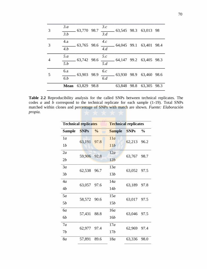
70
3 3.a
63,770 98.7 3.c
63,545 98.3 63,013 98 3.b 3.d
3 4.a
63,765 98.6 4.c
64,045 99.1 63,401 98.4 4.b 4.d
4 5.a
63,742 98.6 5.c
64,147 99.2 63,405 98.3 5.b 5.d
5 6.a
63,903 98.9 6.c
63,930 98.9 63,460 98.6 6.b 6.d
Mean 63,829 98.8 63,848 98.8 63,305 98.3
Table 2.2 Reproducibility analysis for the called SNPs between technical replicates. The
codes a and b correspond to the technical replicate for each sample (1-19). Total SNPs
matched within clones and percentage of SNPs with match are shown. Fuente: Elaboración
propia.
Technical replicates Technical replicates
Sample SNPs % Sample SNPs %
1a 63,191 97.8
11a 62,213 96.2
1b 11b
2a 59,906 92,8
12a 63,767 98.7
2b 12b
3a 62,538 96.7
13a 63,052 97.5
3b 13b
4a 63,057 97.6
14a 63,189 97.8
4b 14b
5a 58,572 90.6
15a 63,017 97.5
5b 15b
6a 57,431 88.8
16a 63,046 97.5
6b 16b
7a 62,977 97.4
17a 62,969 97.4
7b 17b
8a 57,891 89.6 18a 63,336 98.0

71
8b 18b
9a 58,766 90.9
19a 62,223 96.3
9b 19b
10a 63,121 97.7 Mean 61,803 95.8
10b
2.4.2 Intraclonal and pedigree validation
An intraclonal validation was made using the recorded clone information for each sample and
its SNPs profile from the genotyping process. Total samples were correctly assigned with a
probability equal to 1 into the clusters inferred by the analysis (Fig. 2.1). Therefore, SNP
profile for each sample allowed its corresponding clonal group.
Fig. 2.1 Graphical representation for the clustering analysis where heat-colors represent
membership probabilities from 0=white to 1=red for each sample (from 1 to 24) to belong to
the cluster (from 1 to 5) inferred and crosses (+) represent the prior clone-cluster provided to
each samples analyzed. Fuente: Elaboración propia.
Using the data from polymorphic markers within families, the ability of SNPs to verify the
progeny of different families was evaluated. The samples with a total of 90% of SNPs
correctly assigned were considered to be clones correctly generated for its family. Therefore,
samples resulting with an error detected on the SNPs profile above 10% of discrepancy with
Clusters
2 3 4 1 5
24
23
22
21
20
19
18
17
16
15
14
13
12
11
10
9
8
7
6
5
4
3
2
1

72
their parents were not considered to be the progeny of a particular family. A total of 21 clones
distributed between thirteen families showed more than 10% of error rate when comparing
their SNPs panel with those obtained for their parents. There were 53 clones distributed
among 33 families correctly assigned, but only 20 of those families did not have error between
their clones (Fig. 2.2).
Fig. 2.2 Pedigree validation of 74 clones distributed between 33 families. Each family ranged
from one to four clones. Percentage of correctly assigned SNPs is showed in blue bars. Red
bars show discrepancy between clones and their parents. Fuente: Elaboración propia.
2.4.3 Comparison between EUChip60k and GBS technologies
Polymorphic SNPs were identified and compared. In this case, all the 164 clone-samples were
considered for the analysis whatever the pedigree information of each sample was previously
documented. Duplicated SNPs from EUChip60K were removed and only SNPs up to 5% of
missing values were considered for the analysis, where a missing value corresponded to all
those markers without their genotype information from the SNP called. A total of 13,669
SNPs were considered polymorphic with a minimum allele count of five between all samples.
A total of 13,669 polymorphic SNPs was compared with a set of SNPs discovered using GBS
technology from two groups (A and B) of clones of E. globulus. In the case of GBS system,
DNA libraries were sequenced and analyzed by a homemade bioinformatics workflow for
marker discovery using E. grandis as a reference genome for mapping and SNP calling

73
process (data not shown). A total of 2,597 polymorphic SNPs were identified by GBS, and
only 35 were common between both groups. When GBS-SNPs technologies were compared
with the set of polymorphic markers from EUChip60K, 11 and 12 SNPs were common with
the A-GBS and B-GBS group respectively, and one SNP was common between under the 3
conditions. Unique SNPs were also found, where a total of 13,645 SNPs were exclusive for
EUChip, 1,229 and 1,310 SNPs were found for A and B groups respectively. A graphical
representation of this analysis is showed in the Fig. 2.3.
Fig. 2.3 A Venn diagram representing a comparison analysis between polymorphic SNP
markers discovered by the EUChip (EUChip60k) and GBS (A-GBS and B-GBS groups)
technological approaches. Fuente: Elaboración propia.
2.5 DISCUSSION
Fingerprinting is a critical process in plant propagation that has been increasingly assisted by
molecular markers (Nybom et al. 2014). During last years the continuous advances in reduced
DNA re-sequencing and SNP-chips, have resulted in a massive amount of SNPs that have
been fixed in arrays for different crops and non-model species (Yan et al. 2009, Hyten et al.
2010, McCouch et al. 2010, Li et al. 2014) including trees (Livingstone et al. 2015, Bianco et
al.2016).

74
In this study, a set of clones of E. globulus was genotyped with 60K SNPs by the EUChip to
evaluate the opportunity to use this panel of markers in improvement of the information
quality used in the breeding program of the species. The multi-species array displayed had a
high performance to identify polymorphic and informative SNPs for E. globulus, since it was
one of the main species used to create the array. The results obtained are consistent with those
previously reported by Silva-Junior et al. (2015) who reported around 19K polymorphic and
transferable SNPs across Eucalyptus Symphymyrtus subgenus and later reported by Telfer et
al. (2015) the fact that a set of markers selected from EUChip for E. nitens were robust and
informative. When the chip-reproducibility was evaluated comparing biological and technical
replicates, a high percentage of SNPs were correctly matched between samples in both types
of replicates. Also, DNA samples extracted from different laboratories did not show any
difference in the SNP genotyping results. The DNA was extracted using the same protocol but
each protocol had slight modifications according with the laboratory requirements and it did
not have an impact in the analysis. When biological and technical replicates were compared,
there was a slight difference in the percentage of SNPs matched correctly, considering that
DNA was extracted from leaf and bark. Previous studies in our laboratory have shown that
bark-DNA has a considerably lower quality than leaf-DNA (data not shown), using DNA
quality control by fluorometric quantification and SSR-genotyping, but apparently in this
analysis, it would not be affecting the genotyping process. It would not be necessary to have
high quality DNA as previously published by others (Bayés and Gut 2011). The number of
missing values was very consistent across all called samples, differently to those reported in
pine studies where protocols and the quality of DNA had an impact in genotyping (Telfer et al.
2013).
Assignment test performed by SNP marker data was efficient to confirm each group of clones.
There were no intraclonal mislabeling according to this analysis. In agreement with this
finding, reported studies in cacao for a set of 53 SNPs was evaluated and showed a robust and
accurate genotyping for identification of errors between 160 tree clones (Takrama et al 2014).
Commercial clonal plantations are more frequently planted, so if mislabeled or incorrectly
identified clones are carried to the field, the economical losses could be damaging. An error in

75
the genotyping process occurs if an observed genotype for an individual does not correspond
to the true genotype (Bonin et al. 2004) and can be detected by comparing replicate
genotyping (Taberlet et al. 1999). The main causes of genotyping error results either from
variation in DNA sequences, low quantity and quality of DNA, biochemical artefacts or
human errors (Pompanon et al. 2005). Therefore it is a really good alternative to consider
technical replicate samples when a genotyping process is being used, it would reduce
probabilities of discarding samples that they were not really off-types and demonstrate that the
results obtained are reliable. Parentage analysis can also support the assignment test, is our
case, we did not have information about the SNP profile for parents of clones previously
evaluated, however, a different set of samples was used, where parents and their progeny were
genotyped to evaluated the ability of SNP to identify off-type intraclones, verifying genetic
identity and pedigree information. Parent profiles are used as a kind of reference to know if
progeny alleles are or are not from parents. Around 28% of clones were mislabeled, having
more than 10% of SNPs unmatched between parents and progeny. Sometimes, these levels of
mislabeling can arise from contamination of the crosses (Takrama et al. 2012) or missing data.
In this study, we considered more than 10% of unmatched SNPs as clonal misidentification,
however, it is going to depend to the on the number of markers used for genotyping (Wang et
al. 2015). Greenhill et al. (2017) screened 113 clones, represented by 2 or more samples, with
31 SNPs and 24 clones exhibited some kind of mislabeling error.
When polymorphic markers of the EUChip were compared with the set of SNPs obtained from
GBS, a low number of them were common between them. The idea was to identify the exact
same group of SNPs across independent technologies and consider these markers as a more
specific group to E. globulus. However, it is difficult and probably impossible considering the
sequencing techniques as GBS; not having reference haplotypes considering the high level of
heterozygosity and that rare identical by descent (IBD) segments are not available yet (Silva-
Junior et al. 2015).
2.6 CONCLUSION
According with the current study, the use of the EUChip as a fingerprint tool in E. globulus
constitutes a simple, fast and robust technology for clonal identity analysis. The pipeline that

76
has been presented can be applied to any other tree plant scenario. The EUChip method
showed not only a high reproducibility between biological and technical replicates, but it had a
very high efficiency to identify off-type samples within clones using two simple profile SNPs
analysis that could be applied routinely for checking. Those analyses would be more difficult
if a sequencing technique such as GBS was used, considering its lower reproducibility
between samples in Eucalyptus species (De Faria 2012). Moreover, we have to consider that
SNPs can not only be used to fingerprint, since EUChip tool may be applied in marker assisted
breeding strategies as genomic selection, where hundreds of thousands of markers are used to
fixing a prediction model that allows the early genomic estimation of breeding values of
clones. A recent study where EUChip was used for genotyping a set of E. globulus clones,
showed that 12 K polymorphic SNPs were identified with a good predictive ability results
between its models (Duran et al. 2017).
The results have shown a moderate cost-effective way using the EUChip60K, as a new
opportunity in a breeding program of E. globulus. However, it should be stated that further
work needs to be carried out with the EUChip markers panel in a larger set of samples from
the breeding program to validate these results.
2.7 REFERENCES
Bayés M, Gut IG (2011) Overview of genotyping. Molecular Analysis and Genome Discovery
Second Edition 1:23
Bianco L, Cestaro A, Linsmith G, Muranty H, Denancé C et al (2016) Development and
validation of the Axiom® Apple480K SNP genotyping array. The Plant Journal 86:62-
74
Bonin A, Bellemain E, Bronken P, Pompanon F, Brochmann C, Taberlet P (2004) How to
track and assess genotyping errors in population genetics studies. Molecular ecology,
13:3261-3273
Chancerel E, Lamy JB, Lesur I, Noirot C, Klopp C et al (2013) High-density linkage mapping
in a pine tree reveals a genomic region associated with inbreeding depression and
provides clues to the extent and distribution of meiotic recombination. BMC Biology
11:50

77
De Faria, DA, Grattapaglia, D (2014) Milhares de SNPS genotipados por sequenciamento de
alto desempenho (GBS-"Genotyping By Sequencing") em espécies de Eucalyptus.
Heringeriana 6:23-25
Duran R, Isik F, Zapata-Valenzuela J, Balocchi C, Valenzuela S (2017) Genomic predictions
of breeding values in a cloned Eucalyptus globulus population in Chile. Tree Genet
Genomes 13:74. doi:10.1007/s11295-017-1158-4
Elshire RJ, Glaubitz JC, Sun Q et al (2011) A robust, simple genotyping-by-sequencing (GBS)
approach for high diversity species. Plos one 6:e19379.
doi:10.1371/journal.pone.0019379
Faivre‐Rampant P, Zaina G, Jorge V, Giacomello S, Segura V et al (2016) New resources for
genetic studies in Populus nigra: genome‐wide SNP discovery and development of a
12k Infinium array. Molecular ecology resources 16:1023-1036
Geraldes A, Difazio SP, Slavov GT, Ranjan P, Muchero W et al (2013) A 34k SNP
genotyping array for Populus trichocarpa: design, application to the study of natural
populations and transferability to other populus species. Molecular Ecology Resources
13: 306–323
Grattapaglia D, Vaillancourt RE, Shepherd M, Thumma BR, Foley W et al (2012) Progress in
Myrtaceae genetics and genomics: Eucalyptus as the pivotal genus. Tree Genet
Genomes 8: 463–508
Grattapaglia D, Silva OB, Kirst M, de Lima BM, Faria DA, Pappas GJ (2011) High-
throughput SNP genotyping in the highly heterozygous genome of eucalyptus: assay
success, polymorphism and transferability across species. BMC Plant Biology 11: 65
Greenhill R, Mollison E, Dowman C, Johnson L et al (2017) Utility of single nucleotide
polymorphism markers in clonal profiling of Hevea brasiliensis. Acta Horticulturae
429:436
Guichoux E, Lagache L, Wagner S, Chaumeil P, Léger P, Lepais O et al (2011) Current trends
in microsatellite genotyping. Molecular Ecology Resources 11: 591–611. doi:
10.1111/j.1755-0998.2011. 03014.x PMID: 21565126
Hyten DL, Choi IY, Song Q, Specht JE, Carter TE et al (2010) A high density integrated
genetic linkage map of soybean and the development of a 1536 universal soy linkage
panel for quantitative trait locus mapping. Crop Sci 50:960–968.

78
Jombart, T (2008) Adegenet: a R package for the multivariate analysis of genetic markers.
Bioinformatics 24:1403-1405. doi:10.1093/bioinformatics/btn129
Jombart T, Ahmed I (2011) Adegenet 1.3-1: new tools for the analysis of genome-wide SNP
data. Bioinformatics doi: 10.1093/bioinformatics/btr521
Li X, Han Y, Wei Y, Acharya A, Farmer AD et al (2014) Development of an Alfalfa SNP
Array and Its Use to Evaluate Patterns of Population Structure and Linkage
Disequilibrium. Plos one 9: e84329. doi:10.1371/journal.pone.0084329
Livingstone D, Royaert S, Stack C, Mockaitis K, May G (2015) Making a chocolate chip:
development and evaluation of a 6K SNP array for Theobroma cacao. DNA research,
22:279-291
McCouch S, Tung CW, Zhao K, Wright M, Kimball J et al (2010) Development of genome-
wide SNP assays for rice. Breeding Sci 60:524–535
Muranty H, Jorge V, Bastien C, Lepoittevin C, Bouffier L, Sanchez L (2014) Potential for
marker-assisted selection for forest tree breeding: lessons from 20 years of MAS in
crops. Tree Genet Genomes 10:1491–1510. doi: 10.1007/s11295-014-0790-5
Nybom, H, Weising K, Rotter B (2014). DNA fingerprinting in botany: past, present, future
Investigative genetics 5:1. https://doi.org/10.1186/2041-2223-5-1
Oliveros JC (2015) Venny. An interactive tool for comparing lists with Venn's diagrams.
http://bioinfogp.cnb.csic.es/tools/venny/index.html
Pavy N, Gagnon F, Rigault P, Blais S, Deschenes A et al (2013) Development of high- density
SNP genotyping arrays for white spruce (Picea glauca) and transferability to
subtropical and nordic congeners. Molecular Ecology Resources 13: 324–336
Pompanon F, Bonin A, Bellemain E, Taberlet P (2005) Genotyping errors: causes,
consequences and solutions. Nature reviews Genetics 6:847
R Core Team (2013) R: A language and environment for statistical computing. R Foundation
for Statistical Computing, Viena, Austria
Schilling MP, Wolf PG, Duffy AM, Rai HS, Rowe CA et al (2014) Genotyping-by-
sequencing for Populus population genomics: An assessment of genome sampling
patterns and filtering approaches. Plos one 9:e95292.
doi:10.1371/journal.pone.0095292

79
Silva-Junior OB, Faria DA, Grattapaglia D (2015) A flexible multi-species genome-wide 60K
SNP chip developed from pooled resequencing of 240 Eucalyptus tree genomes across
12 species. New Phytol 206:1527–1540. doi: 10.1111/nph.13322
Taberlet P, Waits LP, Luikart G (1999) Noninvasive genetic sampling: look before you leap
Trends Ecol Evol 14:323–327
Takrama J, Dadzie AM, Opoku SY, Padi FK, Adomako B et al (2012) Applying SNP marker
technology in the Cacao breeding programme in Ghana. African Crop Science Journal
20:67–75
Takrama J, Kun J, Meinhardt L, Mischke S, Opuku SY (2014) Verification of genetic identity
of introduced cacao germplasm in Ghana using single nucleotide polymorphism (SNP)
markers. African Journal of Biotechnology 13:2127-2136
Telfer E, Graham N, Stanbra L, Manley T, Wilcox P (2013) Extraction of high purity genomic
DNA from pine for use in a high-throughput Genotyping Platform. New Zealand
Journal of Forestry Science 43:3
Telfer EJ, Stovold GT, Li Y, Silva-Junior OB, Grattapaglia DG, Dungey HS (2015) Parentage
Reconstruction in Eucalyptus nitens Using SNPs and Microsatellite Markers: A
Comparative Analysis of Marker Data Power and Robustness. Plos one 10:e0130601.
doi:10.1371/journal.pone.0130601
Wang B, Tan HW, Fang W, Meinhardt LW, Mischke S, Matsumoto T, Zhang D (2015)
Developing single nucleotide polymorphism (SNP) markers from transcriptome
sequences for identification of longan (Dimocarpus longan) germplasm. Hortic Res
2:14065.
Yan JB, Yang XH, Shah T, Sanchez-Villeda H, Li JS et al (2009) High-throughput SNP
genotyping with the GoldenGate assay in maize. Mol Breed 25:441–451

80
CAPÍTULO III: GENOMIC PREDICTIONS OF BREEDING VALUES IN A CLONED
EUCALYPTUS GLOBULUS POPULATION IN CHILE
Ricardo Durán, Fikret Isik, Jaime Zapata-Valenzuela, Claudio Balocchi, Sofía Valenzuela
3.1 ABSTRACT
In Chile, an intensive Eucalyptus globulus clonal selection program is being carried out to
increase forest productivity for pulp production. A breeding population was used to investigate
the predicted ability of single nucleotide polymorphism (SNP) markers for genomic selection
(GS). A total of 310 clones from 53 families were used. Stem volume and wood density were
measured on all clones. Trees were genotyped at 12 K polymorphic markers using the
EUChip60K genotype array. Genomic best linear unbiased prediction, Bayesian lasso
regression, Bayes B, and Bayes C models were used to predict genomic estimated breeding
values (GEBV). For cross-validation, 260 individuals were sampled for model training and 50
individuals for model validation, using 2 folds and 10 replications each. The average
predictive ability estimates for wood density and stem volume across the models were 0.58
and 0.75, respectively. The average rank correlations were 0.59 and 0.71, respectively. Models
produced very similar bias for both traits. When clones were ranked based on their GEBV,
models had similar phenotypic mean for the top 10% of the clones. The predicted ability of
markers will likely decrease if the models are used to predict GEBV of new material coming
from the breeding program, because of a different marker–trait phase introduced by
recombination. The results should be validated with larger populations and across two
generations before routine applications of GS in E. globulus. We suggest that GS is a viable
strategy to accelerate clonal selection program of E. globulus in Chile.
Keywords E. globulus, Genomic selection, SNP, Predictive ability, Stem volume, Wood
density
Este trabajo fue publicado como: Duran R, Isik F, Zapata-Valenzuela J, Balocchi C,
Valenzuela S (2017) Genomic predictions of breeding values in a cloned Eucalyptus globulus
population in Chile. Tree Genet Genomes 13:74. doi:10.1007/s11295-017-1158-4

81
3.2 INTRODUCTION
The Myrtaceae genus is generally diploid and has smaller genome than the Pinaceae genus
(Neale and Kremer 2011). Eucalyptus species have been widely planted in tropical and
subtropical regions of the world for production of biomass energy, wood and pulp, being one
of the most widely planted species in the world because of its remarkable growth and
adaptability (Eldridge et al. 1993; Doughty 2000; Potts et al. 2004). Since its introduction, the
species has been subject to breeding and selection in many countries to develop locally
adapted populations. The breeding programs aim to select genotypes for superior growth, stem
form, and wood quality (Raymond et al. 1998); therefore, it is a target of genomic research,
especially for the pulp and paper industry (Borralho et al. 1993; Grattapaglia 2004).
Breeding programs have relied on classical genetic evaluation based on pedigree and progeny
testing to predict estimated breeding values (EBV). In Eucalyptus spp., the Brazilian breeding
program is an example of cloning superior selections within full-sib families to improve the
mean of the selected population (Rezende et al. 2013). Although traditional genetic evaluation
system and cloned progeny testing have been successful to improve traits of interests in
Eucalyptus globulus improvement programs, the process takes 12 years to complete and it is
costly. Breeders look for new tools to select superior individuals at lower cost in a shorter time
to make the breeding programs more efficient.
Marker assisted selection (MAS) was evaluated with the objective to increase the selection
efficiency in tree breeding programs for decades. This methodology is based on the detection
of QTLs (quantitative trait loci) controlling the phenotype and use them in breeding programs
to increase the selection process (Muranty et al. 2014). However, marker assisted selection has
not been a useful tool for complex traits due its inability to capture small-effect alleles (Isik
2014; Strauss et al. 1992) and most traits important to forest breeding are complex, controlled
by many genes with small effects (Crosbie et al. 2006). It was suggested that compared to
linkage mapping to detect QTLs, associative mapping could be more efficient to establish
marker–trait associations in outbred species, such as forest trees (Neale and Savolainen 2004).
However, it has been difficult to prove that one specific marker is related to a phenotype
(Weigel and Nordborg 2005; Isik 2014). For example, genome-wide association studies have

82
not been successful to capture a large fraction of phenotypic variance (Thumma et al. 2005;
Grattapaglia and Resende 2011; Cappa et al. 2013). Therefore, this strategy has failed to
impact the improvement of polygenic characteristics of forest species (Zapata-Valenzuela and
Hasbun 2011).
In contrast to MAS, genomic selection (GS) uses a dense marker coverage of genome and
capture the effect of thousands of markers simultaneously (Meuwissen et al. 2001). Today,
with advancements in high-throughput genotyping platforms, GS has been successfully
implemented in cattle breeding and has been widely adapted for other major animal and crop
breeding programs (Hayes et al. 2009; Heffner et al. 2009; Hayes and Goddard 2010; Jannink
et al. 2010; Lin et al. 2014; Meuwissen et al. 2016). The success was mainly attributed to
high-throughput DNA sequencing technologies and dramatic drop in DNA sequencing cost.
GS assumes that, with a high density of markers, some markers would be in linkage
disequilibrium (LD) with at least one QTL distributed on the genome (Goddard and Hayes
2007), so a high level of LD improves the marker-tagged QTL and marker–trait association.
Unlike MAS, GS does not use a subset of markers, rather it analyzes the information of all
markers in a population to explain the genetic variance from markers across the genome
(Heffner et al. 2009; Isik 2014), thus precluding the search for significant marker–trait
association. GS overcomes the problem of mapping association where a limited proportion of
total genetic variation is captured by each individual marker and the marker effects do not
need to exceed a significance threshold to be used to predict breeding values (Hayes et al.
2013; Isik 2014).
GS uses a “training set of individuals” that are phenotyped and genotyped by genome-wide
panel of markers to estimate the marker effects. Then, the model is used to predict breeding
values in validation set for which genotypes, but no phenotypic data are available (Zapata-
Valenzuela et al. 2012). So, these genomic estimated breeding values (GEBV) are predicted
only using the marker information (Goddard and Hayes 2009; Isik et al. 2015). To maximize
the accuracy, the training population must be representative of selection candidates in the
breeding program where GS applied (Heffner et al. 2009; Jonas and de Koning 2013). This
approach can offer greater precision than traditional genetic evaluation, as long as the markers
are in LD with some QTL that are controlling the phenotypic variation (Calus and Veerkamp

83
2007) or markers are capturing genetic relationships better than pedigree-based methods. This
requires thousands of molecular markers to capture a significant proportion of the additive
genetic variance (Heffner et al. 2009). The level of LD between marker and QTL, effective
population size, number of individuals in the training population, marker density, and
heritability of the traits are considered affecting the accuracy of GS (Grattapaglia and Resende
2011; Isik 2014).
Forest trees are among the species most likely to benefit from using genomic information in
breeding programs. Today, sever- al forest tree genomes have been sequenced, including
Populus trichocarpa (Tuskan et al. 2006), Pinus taeda, (Neale et al. 2014), and Eucalyptus
grandis (Myburg et al. 2014). During the last several years, there have been numerous studies
on GS in forest trees species (Zapata-Valenzuela et al. 2012; Resende et al. 2012a, b, c;
Zapata-Valenzuela et al. 2013; Beaulieu et al. 2014a, b; Munoz et al. 2014; El-Dien et al.
2015; Ratcliffe et al. 2015; Bartholomé et al. 2016, Isik et al. 2016). For example, Isik et al.
(2016) analyzed two generations of Pinus pinaster L. breeding population to test the predictive
ability of markers. Bartholomé et al. (2016) analyzed three generations for the same species
for assessment of the prediction accuracy of the GS model within and across generations.
Ratcliffe et al. (2015) explored GS for interior spruce (Picea engelmannii × glauca). Resende
et al. (2012c) reported encouraging results for GS for different species of Eucalyptus. Denis
and Bouvet (2013) used simulated data for Eucalyptus breeding with different levels of
heritability, dominance, and additive variance.
This study is the first to test the utility of GS in E. globulus for prediction of breeding values.
The objectives in this study are to (1) evaluate LD levels between markers by each
chromosome, (2) estimate the genomic relationship from markers, and (3) compare various
statistical methods for genomic estimated breeding values of wood density and volume of E.
globulus clones.
3.3 MATERIALS AND METHODS
3.3.1 Plant material and SNP genotyping by EUChip60K
This study was carried out with a breeding population of E. globulus owned by Forestal
Arauco S.A., Chile. The breeding population consisted of a total of 310 clonal individuals

84
belonging to 40 full-sib families and 13 half-sib families, produced by crossing 23 parents.
Two individuals did not have their parents identified (phenotypic selections). For the DNA
extraction, diploid tissue bark or leaves from each individual were collected. DNA was
purified using the Qiagen kit (Hilden, Germany) according to the manufacturer’s protocol. The
quality and quantity of the DNA were assessed using the Qubit fluorometer (Invitrogen,
Carlsbad, CA, USA). A genome-wide single nucleotide polymorphism (SNP) dataset was
obtained using the EUChip60K system (GeneSeek, USA) proposed by Silva-Junior et al.
(2015). Approximately 64 K SNP loci were filtered and processed to obtain about 12 K SNPs.
These SNPs represent a group of polymorphic markers for E. globulus. SNPs were distributed
across 11 chromosomes (Fig. S3.1). The average number of markers per chromosome was
1136 with a range of 800 to 1564 SNPs per chromosome. Larger chromosomes had more
SNPs than smaller chromosomes. The polymorphic information content (PIC) values were in
the range of 0.090 to 0.375, and heterozygosity values were in a range of 0.09 to 0.50 (Fig.
S3.2).
3.3.2 Experimental design, data collection, and preliminary analysis
In 1990s, superior trees from plantations were grafted for controlled crosses. The clones were
generated from the clonal breeding program of the company, after rooting evaluation. Data for
the clones used in this study were obtained from the database of the breeding program, which
was built as follows: phenotypic data for volume and wood density traits of 3150 eucalypt
trees was assessed in 23 field genetic tests growing in one geographic coastal zone at ages
ranging from 5 to 11 years. The experimental test design was randomized incomplete blocks
with single-tree plots, with border rows. Spacing was 3 × 2 m in all tests. For each tree, the
diameter at breast height (cm) using diameter tape and the total height (m) using a Vertex
hypsometer were recorded. The data were stored in the field using a PSION data logger model
Workabout Pro. Stem volume (m3) was estimated from a general formula for juvenile trees as
volume = 0.00003 × (diameter2) × (height) (Ladrach 1986). The wood density was predicted
by near-infrared (NIR) spectroscopy. A calibration model that included samples of E. globulus
and E. nitens, between 4 and 20 years old, was developed using a partial least-squares
algorithm. This method has been used as a fast method for the estimation of many wood
properties using NIR spectra collected from milled wood chips (Schimleck 2008). For our

85
study, due to limited resources, the phenotypic data were available for 310 genotypes for vol-
ume trait and 231 genotypes were measured for wood density. Clonal EBVs were obtained by
fitting the following linear mixed model:
𝐲 = 𝐗𝐛 + 𝐙𝐮 + 𝐞 (1)
where y is the vector of phenotypic observations (volume and density), b is the vector of the
fixed effects intercept, site and block; u is the vector of random clone effect; e is the vector of
random residuals; and X and Z are the incidence matrices, for the fixed and random effects,
respectively. The random clone effect and the residuals have the expectations of
E(𝒖)~iid(0, σu2) and 𝐸(𝐞)~iid(0, σe
2) . Model to predict EBVs for density was used to
estimate breeding values to samples without density measure. ASReml software (Gilmour et
al. 2009) was used to estimated variance components and solve mixed mod- el equations to
obtain the EBVs for wood density and volume, that what were not highly correlated (Fig. 3.1).
The average broad sense heritability for these tests was 0.29 for volume and 0.46 for wood
density.

86
Fig. 3.1 Histograms(diagonal), scatter plots (lower diagonal), and correlation with p-value
(upper diagonal) between wood density and volume (H0: r = 0). Fuente: Elaboración propia.
3.3.3 Proccesing marker data
Synbreed (Wimmer et al. 2012) package in the R 3.0.2 envi- ronment was used (R Core Team
2013) to process various datasets. A total of 64,639 markers were evaluated. The genotypes
were coded as zero, one, and two for the number of gene content. The frequencies of phased
genotypes 0, 1, and 2 were 0.54, 0.40, and 0.06, respectively. SNPs with a minor allele
frequency of 0.05 or less were discarded from the analysis. SNPs with >10% missing
genotypes were also removed. No duplicated SNPs were found. A total of about 12 K markers
remained after the filtering process. Missing genotypes were imputed using the random
sampling from the marginal allele distribution of the markers. For two possible genotypes
(zero and two values) missing, genotypes were sampled from distribution with probabilities
P(x = 0) = 1-p and P(x = 2) = p, where p is the minor allele frequency of marker j. In the case
of three genotypes (two homozygous and one heterozygous), values were sampled from P(x =
Density
−40 −20 0 20 40
−20
−1
5−
10
−5
05
10
r = 0.25
p < 0.001
−20 −15 −10 −5 0 5 10
−40
−2
00
20
40
●
●
●
●
●
●
●
●
●
●
●
●
●
●
●
●
●
●
●●
●
●
●
●
●
●
●
●
●
●
●
●
●
●
●● ●
●
●●
● ●
●
●●●
●
●
●
●
●
●
●
●●
●
●
● ●●
●
●
●●
●
●
●
●
●
●●
●● ●●●
●●
●
●●
●
●
●●
●
●
●
●●●
●
●●
●●
●
●●
●
●
●●
●
●
●●
● ●●
●
●●
●
●
● ●
●
●
●●
●●
●
●●
●
●
●●
●
●●
●
●
●
●
●
●
●
●●
●
●
●
●●
●
●●● ●
●●
●
●
●
●
●
●
●
●
●●
●●
●
●
●
●●
●
●
●
● ●●●
●
●
●
●
●●
●
●
●
●
●
●
●
●
●
● ●●● ●
●
●
● ● ●●
●●
●
●● ●●
●
●
●
●
●
●●
●●
● ●●
●
●
● ●●
●●
●●
●
●
●
●
●●
●
● ●● ●
●●
●
●
●
●
●
●
●●
●
●
●
●
●
●
●
●●
●
●●
●
● ●
●
●
●
●●
●
●●
● ●
●
●
●
●
●
●●
●
●
●
●
●
●
●
●●
●
●
●
●
● ●
●
●
●
●
●
●●
●●
●
Volume

87
0) = (1 − p)2, P(x = 1) = p(1 − p), and P(x = 2) = p2 distribution assuming Hardy–Weinberg
equilibrium for all loci (Wimmer et al. 2012).
Genetics (Warnes et al. 2013) package in R was used to estimate genotype frequency (the
proportion of each genotype in the population) and allele frequency (proportion of all alleles
that are of the specified type) (White et al. 2007). PIC and heterozygosity were estimated for
each marker to evaluate the discriminatory power of a locus (Guo and Elston 1999). Intra-
chromosomal LD measured as r2 between pairs of loci was calculated using the Synbreed
package (Wimmer et al. 2012). To analyze the LD decay, LD values versus the position of the
markers was plotted for each chromosome. Using the LDheatmap package (Shin et al.
2006), a heat map with the r2 values (from 0 to 1) between pairs of markers was
generated. Physical distance was considered to indicate the total length of the region
analyzed.
3.3.4 Statistical models for genomic prediction
Genomic best linear unbiased prediction (GBLUP), Bayesian Lasso (BLasso), Bayes B, and
Bayes C models were used to predict GEBV. In the GBLUP approach, the additive genetic
relationship matrix derived from pedigree is replaced with the realized genomic relationship
matrix (G) obtained from shared alleles. A matrix of genomic relationship (G) between all
pairs of individuals was computed as follows (VanRaden 2008).
(2)
Where Z is the incidence matrix of markers. Considering the second allele frequency at the
locus i as (pi) and let P be a matrix with the allele frequencies expressed as P = 2(pi − 0.5).
Genomic relationships could better estimate the proportion of chromosome segments shared
by individuals, because high-density genotyping identifies genes identical in state that may be
shared through common ancestors not recorded in the pedigree (Forni et al. 2011). Mixed
model equations were solved to obtain GEBV values as:
G =ZZ '
2 pi (1- pi )å

88
(3)
Where α=σe2/σu
2 is the sum across marker loci 2 ∑pi(1 − pi) times the ratio α = σe2/σa
2 where σa2
is the total genetic variance and σu2 is the additive genetic variance (VanRaden 2008).
Among the whole genome regression models, we used BLasso, Bayes B, and Bayes C. Lasso
regression was initially developed by Tibshirani (1996) to overcome colinearity in multi-
dimensional data. Park and Casella (2008) intro- duced the Bayesian approach to have a
specific shrinkage for each marker effect. Lasso combines variable selection and shrinkage.
Regression coefficients are shrunk towards zero; however, some of the coefficients are shrunk
to exactly zero, which reduces the complexity of the model (Isik et al. 2016). The model has
the form y = xβ + e, and mathematically, Lasso estimates are:
(4)
Where y is the response (phenotype), μ is an intercept, X corresponds the n x p design matrix,
β the p × 1 vector of regression coefficients, e the n × 1 error vector, and λ is reg- ularization
parameter (Isik et al. 2016).
Meuwissen et al. (2001) proposed Bayes A and Bayes B whole genome regression models to
genomic prediction. In Bayes B, the prior assumes the variance of markers equal to zero with
probability π and the rest with probability (1 − π) follows an inverse Χ2 distribution
(Meuwissen et al. 2001). Bayes C is very similar to Bayes B, except for the estimation of the
proportion of SNPs with zero effects (π), assuming a common variance for all fitted markers
effects (Habier et al. 2011; Wolc et al. 2011) which follows a scaled inverse χ2 prior with
degrees of freedom va and scale parameter S2a (Habier et al. 2011). In Bayes C, the mixture
probability π has a prior uniform distribution. The variable π is unknown and is estimated from
the data. Synbreed package (Wimmer et al. 2012) and BGLR package (De los Campos and
Perez Rodriguez 2014) in the R 3.0.2 environment were used to run the models. Results were
visualized with the ggplot2 package (Wickham 2009).
XX´ X´Z
Z´X Z´Z + G-1a
é
ëê
ù
ûú+
b
u
é
ëê
ù
ûú =
X´y
Z´y
é
ë
êê
ù
û
úú

89
3.3.5 Validation of the GS models
To test the predictive power of markers, several cross- validation scenarios were run. The
population was sepa- rated into “training” and “validation” sets. A total of 260 random
individuals were used as training set, and 50 individuals were used as validation set. For the
cross-validation, 2 folds and 10 replications were used. The predictive ability of each fold in
each replication was calculated as the correlation of EBV and GEBV. Spearman’s rank
correlation of each fold within each replication was calculated. Mean squared error (MSE) of
each fold between the EBV and GEBV of validation set was calculated as MSE=1
n∑ (Ŷi-
ni=1
Yi)2. The bias of the model was obtained by regressing the EBV on the GEBV in the
validation set. A regression coefficient of <1 implies inflation of genomic estimated breeding
values and a coefficient of >1 suggests deflation of GEBVs (Wimmer et al. 2012). Finally,
individuals in the validation set were ranked according with their GEBV and the mean EBV of
the 10% best was calculat- ed for each replication.
3.4 RESULTS
3.4.1 LD between pair of markers
LD and descriptive statistics for each chromosome are presented in Table 3.1. The number of
markers by chromosome ranged from 824 for chromosome one to 1564 for chromosome eight.
The LD for each chromosome ranged from zero to one with a mean of 0.029. A scatter plot of
LD between pairs of markers on chromosome eight suggests that LD decays rapidly according
to the physical distance (Fig. 3.2a, b). LD decay scatter plots for all other 11 chromosomes are
in Fig. S3.3. LD is decaying within the first 3 K. Heat maps were used to observe different
levels of r2 between pairs or markers by chromosome (Fig. 3.2c, Fig. S3.4). Heat maps
suggest lack of LD between SNP markers on chromosomes, with some exceptions. The
overall LD across genome suggests that only 0.09% of the LD values were greater than 0.50;
therefore, most markers had lower levels of LD between 0 and 0.50 (Fig. 3.3).

90
Table 3.1 Descriptive statistics of linkage disequilibrium analysis for each chromosome. Total
number of SNPs per chromosome, mean, minimum and maximum LD estimates (r2) are
presented. Fuente: Elaboración propia.
Linkage Disequilibrium (r2)
Chromosome SNPs Mean Minimum Maximum
1 824 0.030 0.00 1
2 1,529 0.028 0.00 1
3 1,344 0.028 0.00 1
4 800 0.030 0.00 1
5 1,208 0.027 0.00 1
6 1,344 0.028 0.00 1
7 1,024 0.028 0.00 1
8 1,564 0.028 0.00 1
9 875 0.033 0.00 1
10 918 0.030 0.00 1
11 1,068 0.031 0.00 1
Mean 1,136 0.029 0.00 1

91
Fig. 3.2 a) Scatter of plot of LD level as coefficient of determination (r2) between pair of SNPs
against the physical distance (pair of bases) for chromosome 8. Smoothed spline represents the
decline of LD. b) LD decay up to 50 K pairwise marker distance for chromosome 8. c) LD
between pair of markers as heat map for the same chromosome. Lines in the diagonal
0.00
0.25
0.50
0.75
1.00
0 10000 20000 30000 40000 50000
Physical distance
LD
r2
a)
c)
b)

92
represent the position of the markers in the chromosome in pair of bases (pb). Color palette
represents the LD level as coefficient of determination (r2) between markers. Fuente:
Elaboración propia.
Fig. 3.3 Frequency of LD estimates (r2) as measured across whole genome. LD between pairs
of markers is largely zero with skewed distribution to the right. Large values of LD might be
due to markers coming from the same loci or from the same contigs. Fuente: Elaboración
propia.
3.4.2 Genetic relationships
Additive genetic relationship matrix from pedigree and genomic relationship matrix from
SNPs are presented in Fig. 3.4. Individuals used in this study are clones belonging to half-sib
and full-sib families, with the exception of two unrelated clones. According to the pedigree
information, individuals had three levels of relationships within the population. Most
individuals had zero coefficients (unrelated) with others within the study population. The
remaining individuals had covariances of 0.25 and 0.50; expected coefficients for half-sibs and
full-sib individuals (or parent–progeny coefficient), respectively. Relationships obtained from
the SNPs markers varied between −0.22 and 0.98. The distribution of relationships between
individuals estimated from markers was continuous rather than discrete. Regarding inbreeding
levels, they were equal to zero from the pedigree-based calculation but they had a distribution
on zero when estimated from shared SNP markers (Fig. S3.5).
2e+06
4e+06
6e+06
0.0 0.4 0.8
r2
Fre
cu
en
cy

93
Fig. 3.4 Expected additive genetic relationship derived from pedigree (top panel) and realized
genetic relationship estimated from SNP markers (bottom panel). Realized genetic
relationships show a continuous distribution compared discrete distribution of relationships
from pedigree. The scale of y-axis is the square root of the frequency. Fuente: Elaboración
propia.
3.4.3 Genomic prediction models for volume and wood density
Statistical models were compared for different fit statistics such as predictive ability of
markers, rank correlation, model bias, residual MSE, and the phenotypic mean of top 10%
individuals based on ranking of GEBV. The summary statistics from cross-validation are
presented in the box plots (Fig. 3.5). The horizontal lines in the box plots are the median of the
prediction ability values from different sets of validation sets. The vertical lines extending
from the boxes show the range of prediction abilities of the models (Fig. 3.5). For wood
density, the predictive ability of GBLUP (mean 0.63) and BLasso (mean 0.61) was higher than
Bayesian models (0.54) (Fig. 3.5). For volume, the predictive ability of GBLUP (mean 0.78)
0
10000
20000
30000
0
10000
20000
30000
Add
itive
Re
aliz
ed
−0.2 0.0 0.2 0.4 0.6
Coefficients
Fre
cu
en
cy

94
and Bayes B (mean 0.76) was higher than BLasso (0.73) and Bayes C (0.72) (Fig. 3.5). For
wood density, BLasso had a narrower distribution, while for volume, GBLUP had the
narrowest distribution of predicted ability values.
Rank correlations from different statistical models followed similar patterns as predicted
ability values (Fig. 3.5). The mean rank correlation for density (0.62) from GBLUP and
BLasso models (0.61) was higher than the mean rank correlations from Bayesian models (0.57
and 0.56). Although symmetric, Bayes C validation samples produced a large variation of rank
correlations for wood density. The mean rank correlation for volume (0.74) from GBLUP and
Bayes B models (0.73) was higher than the mean rank correlations from BLasso (0.70) and
Bayes C (0.67). In terms of the distribution, we observed mixed results. For example, for
density, GBLUP and BLasso had a narrower distribution of rank correlations, while for
volume, Bayes C had the narrowest distribution.

95
Fig. 3.5 Evaluation of statistical models (GLUP, BLasso, Bayes B, and Bayes C) using
random sampling of 50 individuals as the validation set with 2 folds and 10 replications for
wood density and volume. The box plots show the distribution of predictive ability of
markers (upper panel) and rank correlation (lower panel) from validation sets. The thick
vertical lines are the median. Fuente: Elaboración propia.
The relationships between GEBV and EBV for wood density and volume are illustrated in Fig.
3.6, where small blue dots are the relationships between direct GEBV and EBV in the training
set, whereas the larger red dots are the relationships between GEBV and EBV for a one of the
validation sets by GBLUP. The scatter plots show that the correlation between GEBV and
EBV for wood density was 0.6 and for volume was 0.73, respectively, for both validation set.
Correlation between direct GEBV and EBV (training set) for both traits was over 0.90.
Density Volume
●
●
●
●
●
●
●
0.4
0.6
0.8
0.4
0.6
0.8
Pre
dic
tive
_a
bility
Ra
nk_
co
rrela
tion
GBLUP BLasso BayesB BayesC GBLUP BLasso BayesB BayesC

96
Fig. 3.6 Predictive ability of SNP markers for wood density and volume in a validation set
(50 random samples) using the GLUP statistical model. The smaller blue dots are direct
GEBV and EBV of the training set with a correlation of r = 0.98 for volume and r = 0.99 for
density. The bigger red dots represent the relationship between GEBV (y- axis) and EBV (x-
axis) of the validation set. Fuente: Elaboración propia.
Several other model fit statistics are given in Table S3.1. Bayes B and Bayes C models had
higher density means (3.8) of the best 10% individuals when ranked for GEBV. GBLUP and
BLasso both had a mean of 3.5 for wood density for the top 10% individuals. The bias from
regressing the GEBV on EBV of density was >1 for the GBLUP and <1 for Bayes B. Other
two models did not have bias (mean slope was one for both models). For volume, the mean of
the best 10% individuals from models were the same. BLasso had a large bias (b>1) for
volume, whereas others had the same smaller bias (1.1).
3.5 DISCUSSION
3.5.1 Linkage disequilibrium
This is the first empirical study for GS in a clonal breeding population of E. globulus. We
detected an average LD of 0.029 when averaged across 11 chromosomes. LD is one of the
factors that affect genomic selection accuracy (Hayes et al. 2009). In forest tree species, LD is
low and decays rapidly according to increasing distance between pairs of markers (Neale and
Savolainen 2004; Isik et al. 2016). Genome recombination and nucleotide diversity have a
direct impact on the LD degree (Silva-Junior and Grattapaglia 2015). Higher LD decay rate
● ●
● ●
●
●
●
●
●
●●
●
● ●●
●
●
●
●
●
●
●
●
●
●●
●
●
●
●
●
●
●
●
●
●
●
●●
●
●
●
●
●
●
●●
●
●
●
●
●
●
●●
●
●
●
●
●
●
●
●
●
●
●●
●
●
●
●
●
●●
●
●
●
●
●
●
●
●
●
●
●●
●
●
●
● ●
●
● ●●
●
●
●
●
●●
●
●
●
●
●
●
●
●
●
●
●
●
●
●
●
●
●
●
●
●
●
●
●
●●
●
●●
●
●●
●
●
●
●
●●
●●
●
●
●
●
●
●
●
●
●
●
●
●
●
●
●
●
●
●
●
●
●
●
●
●●
●
●
●
●●●●
●
●
●
●
●
●
●
●
●
●
●
●
●
●
●
●
●
●
●
●
●
●
●
●
●
●
●
●●
●
●
●●● ●●
●
●
●
●
●
●
●●
●
●
●
●
●
●
●
●●
●
●●
●
●
●
●●
●
●●
●
●
●
●
●●
●
●
●
●
●
●
●
●
●
●
●
●
●
●
●●
●●
●
●
●
●
●●
●
●
●
●
●
●
●
●
●
● ●
●
●
●
●
●
●●
●● ●
●
●●● ●
●
●
●
●
●
●
●
●
●
●
●
●
●
●
●
●●●
●
●
●
●
●●
●
●
●
●
●
●
●
●
●
● ●
●
●
●
●
●
●●
●
● ●
●
●
●● ●
●
●
●
●
●
●
●
●
●
●
●
●
●
●
●
●●●
r= 0.6
−5
0
5
−20 −10 0 10
EBV
GE
BV
Density
●
●
●
●●●
●
●
●
●
●
●
● ●
●
●
●
●
●
●
●
●
●
●●●
●
●● ●
●
●
●
●
●
●
●
●
● ●
●
●
●
●
●
●
●
●
●
●
●
●●
●
●
●
●
●
●●
●
●
●
●
●●
●
●
●
●
●
● ●
●
●
●
●
●
●
●
●
●
●
●●
●●●
●
●
●
●
●
●
●
●
●
●
●
●
●
●
●●
●
●
●
●
●●
●
●
●
●
●
●
●
●●
●
●● ●●
●
●
●
●
●●
● ●
●
● ●
●
●●
●
●●●
● ●
●
●
●
●●
●
●
●
●
●●
●
●●●
●
●
●
●
●
●
●
●●
●
●
●
●
●
●
●
●●
●●
●
●
●●
●
●
●
●
●
●
●
●
●
● ●
●●
●
●
●
●
●
●
●●
●
●
●
●
●
●
●
●
●
●
●
●
●
●
●
●
●
●
●
●
●
●
●
●
●
●
●
●
●●
●
●●
●
●
●●
●
●
●●
●
●
●●
●
●
●
●
●
●
●
●
●
●●
●
●
●
●●
●
●
●
●
●●
●
●
●
●●
●
●
●
●
●
●
●
●
●
●●●
●
●
●
●
●
●
●
●
●
●
●
●
●
●
●
●
●
●
●
●
●
●
●
●
●
●●
●
●
●
●
●●
●
●
●
●●
●
●
●
●
●
●
●
●
●
●●●
●
●
●
●
●
●
●
●
●
●
●
●
●
●
●
●
●
●
●
●
●
●
r= 0.73
−20
0
20
40
−25 0 25 50
EBV
GE
BV
Volume

97
has been demonstrated in genes sequenced for some forest species; however, recent studies
have described a lower LD decay than expected considering sequencing technologies for
whole genome. For example in E. globulus (Thavamanikumar et al. 2011) and E. grandis
(Faria and Grattapaglia unpublished from Grattapaglia and Kirst 2008), a few candidate genes
were analyzed and the LD decay rate is higher than using genotyping whole genome in E.
grandis (Silva-Junior and Grattapaglia 2015). In some cases, a few groups of SNPs in LD
could be detected in some chromosomes. Probably, considering the small effective population
size and the SNPs coverage on the genome, both factors increase the possibility to find some
markers closer to each other in the same locus across the chromosome. Scatter plots by
chromosome displayed that when the distance between markers is longer, LD levels are lower.
Similar results were reported in P. trichocarpa from candidate genes and whole genome
sequencing (Slavov et al. 2012). Isik et al. (2016) eported intra-chromosomal LD of 0.01 in
maritime pine. When they corrected LD for the genomic relationships derived from markers, it
was even smaller (0.006).
3.5.2 Genomic relationships
Genetic relationships based on shared markers between relatives show a continuous
distribution and are more realistic compared to the expected genetic relationships derived from
pedigree (Fig. 3.4). Genomic relationship can vary depending on the number of alleles shared
between individuals. For example, full-sib trees share more genes that are identical by descent
or identical by state than half-sib trees. When many markers are available and when there are
large numbers of individuals in the population, they can be used to estimate the true
relationships among relatives (Powell et al. 2010) and they can provide more realistic
estimates about the shared genome between individuals. Lower diagonal elements in the
matrix were centered at 0.5 and 0.25 for individuals from full-sib and half-sib families,
respectively, corresponding with the expected values derived from pedigree (Simeone et al.
2011). Therefore, only two peaks should be expected with the genomic relationship frequency
(Fig. 3.4) while other peaks closer to zero with positive and negative values are present as
well. Those values represent individuals which do not have any relationship in the population,
because they are not either full-sib or half-sib trees (Munoz et al. 2014). Depending on
whether the values are close to zero, positive or negative, we can say that the individuals are
more or less similar than expected or they are sharing fewer or larger number of alleles than

98
expected from the allele frequencies (Bartholomé et al. 2016). When the genomic relationship
is closer to one (upper diagonal values), these individuals can be seen as biological replicates
(ramets). They can also be attributed to errors in the sampling or genotyping errors.
3.5.3 Predicted ability of markers
We detected high predictive ability of markers, especially for stem volume (0.73) in our E.
globulus population. Rank correlations between EBV and GEBV were also high. As in other
previous studies (Munoz et al. 2014; Isik et al. 2016), the population was randomly split into
training and validation sets for cross-validation. In such cross-validation scenarios, the
marker–QTL phase does not change and thus the results in this study are proof of concept. The
marker–QTL phase can drastically change once the population goes through a cycle of
breeding due to recombination (Isik 2014). If the model developed in this study is used to
predict GEBV of a new generation, the predicted ability values may go down. The small
sample size for the training and validation set has caused a fold-to-fold variation represented
as the difference between maximum and minimum predictive ability values for each model
evaluated. Considering that we only have 310 samples for the analysis, splitting the total
population in more and less samples for training and validation set, respectively, would be
difficult. It is known that considering a large size for training population, the accuracy of the
prediction increases; however, the relatedness between training and validation set is also
important. Bartholomé et al. (2016) compared prediction accuracies across different sampling
strategies showing more variation when the validation set was sampled between half-sib
families comparing with random and within full-sib families as validation sets. Therefore, if
we consider that in our study a random split was done, it is expected that the fold variation
decreases with a high level of relatedness. However, relatedness between cross-validation sets
is not just affecting the level of variation, but it is affecting the level of prediction as well.
With a lower relatedness between training and validation set, predictive abilities of the models
could decrease as well. Different studies reported in forest tree species have shown that both
higher relatedness between training and validation set and a deep pedigree in the training set
can increase the prediction accuracy. Isik et al. (2016) reported a marginal advantage when
individuals from G0 and G1 generation were used as training set over when population was
split randomly in two sets. Bartholomé et al. (2016) showed that when level of relatedness
between training and validation was increased, the mean of the prediction accuracy was

99
increased as well. They also assessed the accuracy over generations using grandparents and
parents as a training set to predict the descendants, showing high accuracy with a range of
0.70–0.85 depending of the trait evaluated. Beaulieu et al. (2014b) evaluated accuracy across
different test sites and breeding groups by cross-validation analysis for wood quality and
growth traits reporting that when there is a strong relatedness between training and validation
set, prediction accuracy was high and moderately high depending of the traits, and it decrease
when relatedness are removed between training and validation set. The underlying reasons for
high accuracy of GEBV is attributed to better capturing genetic relationships rather than
exploiting the LD between marker-tagged QTLs and traits (Zapata-Valenzuela et al. 2012; Isik
2014; Isik et al. 2016). With dense marker coverage and large population with deep pedigree,
markers may be able to exploit LD between phenotype and trait loci in the future generations.
In loblolly pine, an average accuracy of 0.56 and 0.36 from two random sampling methods
were reported for volume (Zapata-Valenzuela et al. 2013). Resende et al. (2012b) reported a
predicted accuracy from 0.67 to 0.77 for wood density in the same species with a heritability
of 0.09 using four different methods. Similar prediction accuracies for growth and wood
density were reported for white spruce (Beaulieu et al. 2014a, b). In Eucalyptus spp.,
predictive ability and accuracy of GS were from 0.38 to 0.60 and from 0.55 to 0.88,
respectively, for four different traits in two elite breeding populations (Resende et al. 2012c).
It is true that EBVs of individuals predicted by BLUP are shrunk towards the parental average
and towards the population mean. The amount of shrinkage is a function of heritability. Isik et
al. (2016) suggested that if the experimental unit is a family or a clone with multiple data
points, the EBVs are not regressed as much. Family mean and clone mean heritability
estimates usually are much larger than individual tree heritabilities. They used the family EBV
and family raw means in a maritime pine population as phenotype and did not find any
noticeable difference for predictive abilities.
3.5.4 Effect of heritability
Wood density is one of the most important traits affecting quality of pulp. In Eucalyptus spp.,
studies reported higher heritability for wood density than growth traits (Borralho et al. 1992;
Apiolaza et al. 2005; Hamilton and Potts 2008). Heritability is considered one of the important
factors affecting the response to selection (Falconer and Mackay 1996). Therefore, breeders
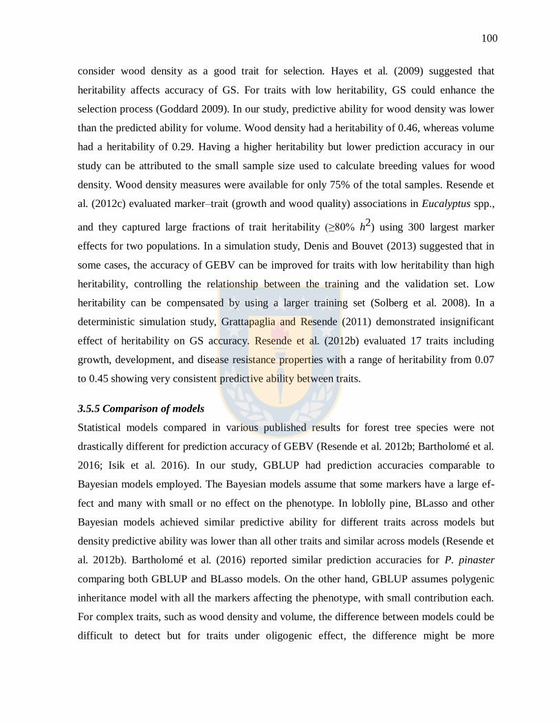
100
consider wood density as a good trait for selection. Hayes et al. (2009) suggested that
heritability affects accuracy of GS. For traits with low heritability, GS could enhance the
selection process (Goddard 2009). In our study, predictive ability for wood density was lower
than the predicted ability for volume. Wood density had a heritability of 0.46, whereas volume
had a heritability of 0.29. Having a higher heritability but lower prediction accuracy in our
study can be attributed to the small sample size used to calculate breeding values for wood
density. Wood density measures were available for only 75% of the total samples. Resende et
al. (2012c) evaluated marker–trait (growth and wood quality) associations in Eucalyptus spp.,
and they captured large fractions of trait heritability (≥80% h2) using 300 largest marker
effects for two populations. In a simulation study, Denis and Bouvet (2013) suggested that in
some cases, the accuracy of GEBV can be improved for traits with low heritability than high
heritability, controlling the relationship between the training and the validation set. Low
heritability can be compensated by using a larger training set (Solberg et al. 2008). In a
deterministic simulation study, Grattapaglia and Resende (2011) demonstrated insignificant
effect of heritability on GS accuracy. Resende et al. (2012b) evaluated 17 traits including
growth, development, and disease resistance properties with a range of heritability from 0.07
to 0.45 showing very consistent predictive ability between traits.
3.5.5 Comparison of models
Statistical models compared in various published results for forest tree species were not
drastically different for prediction accuracy of GEBV (Resende et al. 2012b; Bartholomé et al.
2016; Isik et al. 2016). In our study, GBLUP had prediction accuracies comparable to
Bayesian models employed. The Bayesian models assume that some markers have a large ef-
fect and many with small or no effect on the phenotype. In loblolly pine, BLasso and other
Bayesian models achieved similar predictive ability for different traits across models but
density predictive ability was lower than all other traits and similar across models (Resende et
al. 2012b). Bartholomé et al. (2016) reported similar prediction accuracies for P. pinaster
comparing both GBLUP and BLasso models. On the other hand, GBLUP assumes polygenic
inheritance model with all the markers affecting the phenotype, with small contribution each.
For complex traits, such as wood density and volume, the difference between models could be
difficult to detect but for traits under oligogenic effect, the difference might be more

101
important. Results from our study and previous published results (Zapata-Valenzuela et al.
2013; Isik et al. 2016) suggest that GBLUP can be used for routine data analysis in a tree
breeding program. As GBLUP models follow the traditional linear mixed model structure,
they would account for heterogeneous covariance structures and genotype by environment
interactions, especially in forestry where contrasting site types are commonly used and
multiple traits are evaluated. Isik (2014) and Grattapaglia (2014) suggest that GS models are
likely to be population specific.
3.6 CONCLUSIONS
This study is the first to test the predictive ability of markers in a clonal breeding population of
E. globulus in Chile. The overall LD was low, but it was higher than LD estimates reported in
P. pinaster. Predictive ability of markers was encouraging for both traits analyzed, wood
density, and volume. The study is a first proof-of-concept experiment based on a small sample
size of trees (310) composed of one generation. The results should be validated with a larger
set of individuals, preferably across two generations. The predicted ability will likely decrease
if the models are used to predict GEBV of new material coming from the breeding program,
because of a different marker–trait phase introduced by recombination. The GBLUP model
represents a good alternative, drawing the realized genetic relationships among relatives and
use them in predicting their GEBVs as a complementary tool to assist the selection criteria of
the best genotypes for propagation and deployment of the breeding program.
3.7 REFERENCES
Apiolaza LA, Raymond CA, Yeo BJ (2005) Genetic variation of physical and chemical wood
properties of Eucalyptus globulus. Silvae Genet 54:160–165
Bartholomé J, Van Heerwaarden J, Isik F, Boury C, Vidal M, Plomion C, Bouffier L (2016)
Performance of genomic prediction within and across generations in maritime pine. BMC
Genomics 17:604. doi: 10.1186/s12864-016-2879-8
Beaulieu J, Doerksen T, Clément S, MacKay J, Bousquet J (2014a) Accuracy of genomic
selection models in a large population of open-pollinated families in white spruce.
Heredity 113:343–352. doi:10.1038/hdy.2014.36

102
Beaulieu J, Doerksen TK, MacKay J, Rainville A, Bousquet J (2014b) Genomic selection
accuracies within and between environments and small breeding groups in white
spruce. BMC Genomics 15:1048. doi:10.1186/1471-2164-15-1048
Borralho NMG, Cotterill PP, Kanowski PJ (1992) Genetic parameters and gains expected
from selection for dry weight in Eucalyptus globulus ssp. globulus in Portugal. For Sci
38:80–94
Borralho NMG, Cotterill PP, Kanowski PJ (1993) Breeding objectives for pulp production of
Eucalyptus globulus under different industrial cost structures. Can J For Res 23:648–
656
Calus MPL, Veerkamp RF (2007) Accuracy of breeding values when using and ignoring the
polygenic effect in genomic breeding value estimation with a marker density of one
SNP per cM. J Anim Breed Genet 124:362–368. doi:10.1111/j.1439-
0388.2007.00691.x
Cappa EP, El-Kassaby YA, Garcia MN, Acuña C, Borralho NM, Grattapaglia D, Poltri SNM
(2013) Impacts of population structure and analytical models in genome-wide
association studies of com- plex traits in forest trees: a case study in Eucalyptus
globulus. PLoS One 8:e81267. doi:10.1371/journal.pone.0081267
Core Team R (2013) R: a language and environment for statistical com- puting. R Foundation
for Statistical Computing, Viena
Crosbie TM, Eathington SR, Johnson GR, Edwards M, Reiter R, Stark S, Mohanty RG,
Oyervides M, Buehler RE, Walker AK, Dobert R, Delannay X, Pershing, JC, Hall MA,
Lamkey KR (2006) Plant breeding: past, present, and future. In: Lamkey KR, Lee M
(eds.) Plant breeding: the Arnel R. Hallauer International Symposium. Blackwell, pp
3–50
De los Campos G, Perez Rodriguez P (2014) BGLR: Bayesian general- ized linear regression.
R package version 1.0.3
Denis M, Bouvet JM (2013) Efficiency of genomic selection with models including
dominance effect in the context of Eucalyptus breeding. Tree Genet Genomes 9:37–51.
doi:10.1007/s11295-012-0528-1
Doughty RW (2000) The eucalyptus: a natural and commercial history of the gum tree.
Baltimore, Maryland

103
El-Dien OG, Ratcliffe B, Klápšte J, Chen C, Porth I, El-Kassaby YA (2015) Prediction
accuracies for growth and wood attributes of in- terior spruce in space using
genotyping-by-sequencing. BMC Genomics 16:1. doi:10.1186/s12864-015-1597-y
Eldridge KG, Davidson J, Harwood CE, van Wyk G (1993) Eucalypt domestication and
breeding. Clerendon Press, Oxford
Falconer DS, Mackay TFC (1996) Introduction to quantitative genetics, Fourth edn. Longman
Group, Ltd, Essex, p 464
Forni S, Aguilar I, Misztal I (2011) Different genomic relationship ma- trices for single-step
analysis using phenotypic, pedigree and geno- mic information. Genet Sel Evol 43:1.
doi:10.1186/1297-9686-43-1
Gilmour AR, Gogel BJ, Cullis BR, Thompson R (2009). ASReml user guide release 3.0. VSN
International Ltd, Hemel Hempstead, HP1 1ES, United Kingdom
Goddard M (2009) Genomic selection: prediction of accuracy and maximisation of long term
response. Genetica 136:245–257. doi: 10.1007/s10709-008-9308-0
Goddard ME, Hayes BJ (2007) Genomic selection. J Anim Breed Genet 124:323–330.
doi:10.1111/j.1439-0388.2007.00702.x
Goddard ME, Hayes BJ (2009) Mapping genes for complex traits in domestic animals and
their use in breeding programmes. Nat Rev Genet 10:381–391. doi:10.1038/nrg2575
Grattapaglia D (2004) Integrating genomics into Eucalyptus breeding. Genet Mol Res 3:369–
379
Grattapaglia D (2014) Breeding Forest trees by genomic selection: current progress and the
way forward. In: Tuberosa R, Graner A, Frison E (eds) Genomics of plant genetic
resources. Springer, Dordrecht, pp 651–682
Grattapaglia D, Kirst M (2008) Eucalyptus applied genomics: from gene sequences to
breeding tools. New Phytol 179:911–929. doi:10.1111/ j.1469-8137.2008.02503.x
Grattapaglia D, Resende MDV (2011) Genomic selection in forest tree breeding. Tree Genet
Genomes 7:241–255. doi:10.1007/s11295-010-0328-4
Guo X, Elston RC (1999) Linkage information content of polymorphic genetic markers. Hum
Hered 49:112–118. doi:10.1159/000022855
Habier D, Fernando RL, Kizilkaya K, Garrick DJ (2011) Extension of the Bayesian alphabet
for genomic selection. BMC Bioinformatics 12:1. doi:10.1186/1471-2105-12-186

104
Hamilton MG, Potts BM (2008) Eucalyptus nitens genetic parameters. NZ J For Sci 38:102–
119
Hayes B, Goddard M (2010) Genome-wide association and genomic selection in animal
breeding. Genome 53:876–883. doi:10.1139/G10-076
Hayes BJ, Bowman PJ, Chamberlain AJ, Goddard ME (2009) Invited review: genomic
selection in dairy cattle: progress and challenges. J Dairy Sci 92:433–443.
doi:10.3168/jds.2008-1646
Hayes BJ, Cogan NO, Pembleton LW, Goddard ME, Wang J, Spangenberg GC, Forster JW
(2013) Prospects for genomic selection in forage plant species. Plant Breed 132:133–
143. doi:10.1111/pbr.12037
Heffner EL, Sorrells ME, Jannink JL (2009) Genomic selection for crop improvement. Crop
Sci 49:1–12. doi:10.2135/cropsci2008.08.0512
Isik F (2014) Genomic selection in forest tree breeding: the concept and an outlook to the
future. New For 45:379–401. doi:10.1007/s11056-014-9422-z
Isik F, Kumar S, Martínez-García PJ, Iwata H, Yamamoto T (2015) Chapter three—
acceleration of forest and fruit tree domestication by genomic selection. In: Plomion C,
Adam-Blondon AF (eds) Advances in botanical research. Academic Press, pp 93–124.
doi: 10.1016/bs.abr.2015.05.002
Isik F, Bartholomé J, Farjat A, Chancerel E, Raffin A, Sanchez L, Plomion C, Bouffier L
(2016) Genomic selection in maritime pine. Plant Sci 242:108–119.
doi:10.1016/j.plantsci.2015.08.006
Jannink JL, Lorenz AJ, Iwata H (2010) Genomic selection in plant breed- ing: from theory to
practice. Brief Funct Genomics 9:166–177. doi: 10.1093/bfgp/elq001
Jonas E, de Koning DJ (2013) Does genomic selection have a future in plant breeding? Trends
Biotechnol 31:497–504. doi:10.1016/j. tibtech.2013.06.003
Ladrach WE (1986) Comparaciones entre procedencias de siete coníferas en la Zona Andina
al finalizar ocho años. Informe de investigación Smurfit Carton Colombia 105:8
Lin Z, Hayes BJ, Daetwyler HD (2014) Genomic selection in crops, trees and forages: a
review. Crop Pasture Sci 65:1177–1191
Meuwissen THE, Hayes BJ, Goddard ME (2001) Prediction of total genetic value using
genome-wide dense marker maps. Genetics 157:1819–1829

105
Meuwissen T, Hayes B, Goddard M (2016) Genomic selection: a para- digm shift in animal
breeding. Anim Front 6:6–14. doi:10.2527/af. 2016-0002
Munoz PR, Resende MFR, Huber DA, Quesada T, Resende MDV, Neale DB, Wegrzyn JL,
Kirst M, Peter GF (2014) Genomic relationship matrix for correcting pedigree errors in
breeding populations: impact on genetic parameters and genomic selection accuracy.
Crop Sci 54: 1115–1123. doi:10.2135/cropsci2012.12.0673
Muranty H, Jorge V, Bastien C, Lepoittevin C, Bouffier L, Sanchez L (2014) Potential for
marker-assisted selection for forest tree breed- ing: lessons from 20 years of MAS in
crops. Tree Genet Genomes 10:1491–1510. doi:10.1007/s11295-014-0790-5
Myburg AA, Grattapaglia D, Tuskan GA et al (2014) The genome of Eucalyptus grandis.
Nature 510:356–362
Neale DB, Kremer A (2011) Forest tree genomics: growing resources and applications. Nat
Rev Genet 12:111–122. doi:10.1038/nrg2931
Neale DB, Savolainen O (2004) Association genetics of complex traits in conifers. Trends
Plant Sci 9:325–330. doi:10.1016/j.tplants.2004.05.006
Neale DB, Wegrzyn JL, Stevens KA et al (2014) Decoding the massive genome of loblolly
pine using haploid DNA and novel assembly strategies. Genome Biol 15:R59.
doi:10.1186/gb-2014-15-3-r59
Park T, Casella G (2008) The Bayesian lasso. J Am Stat Assoc 103:681– 686.
doi:10.1198/016214508000000337
Potts BM, Vaillancourt RE, Jordan G et al (2004) Exploration of the Eucalyptus globulus gene
pool. In: Borralho NMG, Pereira JS, Marques C, Coutinho J, Madeira M, Tomé M
(eds) Eucalyptus in a changing world proceedings of IUFRO Conference, 11–15
October Aveiro, Portugal. RAIZ, Instituto Investigação de Floresta e Papel, pp 46–61
Powell JE, Visscher PM, Goddard ME (2010) Reconciling the analysis of IBD and IBS in
complex trait studies. Nat Rev Genet 11:800–805. doi:10.1038/nrg2865
Ratcliffe B, El-Dien OG, Klápšte J, Porth I, Chen C, Jaquish B, El- Kassaby YA (2015) A
comparison of genomic selection models across time in interior spruce (Picea
engelmannii × glauca) using unordered SNP imputation methods. Heredity 115:547–
555. doi:10. 1038/hdy.2015.57

106
Raymond CA, Banham P, MacDonald AC (1998) Within tree variation and genetic control of
basic density, fibre length and coarseness in Eucalyptus regnans in Tasmania. Appita J
51:299–305
Resende MFR, Muñoz P, Acosta JJ, Peter GF, Davis JM, Grattapaglia D, Resende MDV,
Kirst M (2012a) Accelerating the domestication of trees using genomic selection:
accuracy of prediction models across ages and environments. New Phytol 193:617–
624. doi:10.1111/j. 1469-8137.2011.03895.x
Resende MFR, Muñoz P, Resende MDV, Garrick DJ, Fernando RL, Davis JM, Jokela EJ,
Martin TA, Peter GF, Kirst M (2012b) Accuracy of genomic selection methods in a
standard data set of loblolly pine (Pinus taeda L.) Genetics 190:1503–1510. doi:10.
1534/genetics.111.13702
Resende MDV, Resende MFR, Sansaloni CP, Petroli CD, Missiaggia AA, Aguiar AM, Abad
JM, Takahashi EK, Rosado AM, Faria DA, Pappas GJ, Kilian A, Grattapaglia D
(2012c) Genomic selection for growth and wood quality in Eucalyptus: capturing the
missing heritability and accelerating breeding for complex traits in forest trees. New
Phytol 194:116–128. doi:10.1111/j.1469-8137.2011.04038.x
Rezende GDSP, de Resende MDV, de Assis TF (2013) Eucalyptus breeding for clonal
forestry In: Fenning T (ed). Challenges and opportunities for the world’s forests in the
21st century. Netherlands, pp 393–424
Schimleck LR (2008) Near infrared spectroscopy: a rapid, non- destructive method for
measuring wood properties and its applica- tion to tree breeding. N Z J For Sci 38:14–
35
Shin JH, Blay S, McNeney B, Graham J (2006) LDheatmap: an R function for graphical
display of pairwise linkage disequilibria between single nucleotide polymorphisms. J
Stat Softw 16. doi:10.18637/jss.v016.c03\
Silva-Junior OB, Grattapaglia D (2015) Genome-wide patterns of recom- bination, linkage
disequilibrium and nucleotide diversity from pooled resequencing and single
nucleotide polymorphism genotyp- ing unlock the evolutionary history of Eucalyptus
grandis. New Phytol 208:830–845. doi:10.1111/nph.13505

107
Silva-Junior OB, Faria DA, Grattapaglia D (2015) A flexible multi- species genome-wide 60K
SNP chip developed from pooled resequencing of 240 Eucalyptus tree genomes across
12 species. New Phytol 206:1527–1540. doi:10.1111/nph.13322
Simeone R, Misztal I, Aguilar I, Legarra A (2011) Evaluation of the utility of diagonal
elements of the genomic relationship matrix as a diagnostic tool to detect mislabelled
genotyped animals in a broiler chicken population. J Anim Breed Genet 128:386–393.
doi:10.1111/j.1439-0388.2011.00926.x
Slavov GT, DiFazio SP, Martin J, Schackwitz W, Muchero W et al (2012) Genome
resequencing reveals multiscale geographic structure and ex- tensive linkage
disequilibrium in the forest tree Populus trichocarpa. New Phytol 196:713–725.
doi:10.1111/j.1469-8137.2012.04258.x
Solberg TR, Sonesson AK, Woolliams JA, Meuwissen THE (2008) Genomic selection using
different marker types and densities. J Anim Sci 86:2447–2454. doi:10.2527/jas.2007-
0010
Strauss SH, Lande R, Namkoong G (1992) Limitations of molecular-marker- aided selection
in forest tree breeding. Can J For Res 22:1050–1061
Thavamanikumar S, McManus LJ, Tibbits JFG, Bossinger G (2011) The significance of single
nucleotide polymorphisms (SNPs) in Eucalyptus globulus breeding programs. Aust For
74:23–29. doi: 10.1080/00049158.2011.10676342
Thumma BR, Nolan MF, Evans R, Moran GF (2005) Polymorphisms in cinnamoyl CoA
Reductase (CCR) are associated with variation in microfibril angle in Eucalyptus spp.
Genetics 171:1257–1265. doi: 10.1534/genetics.105.042028
Tibshirani R (1996) Regression shrinkage and selection via the lasso. J R Stat Soc B
Methodol:267–288
Tuskan GA, DiFazio S, Jansson S et al (2006) The genome of black cottonwood, Populus
trichocarpa (Torr. & Gray). Science 313: 1596–1604. doi:10.1126/science.1128691
VanRaden PM (2008) Efficient methods to compute genomic predictions. J Dairy Sci
91:4414–4423. doi:10.3168/jds.2007-0980
Warnes G, Gorjanc G, Leisch F, Man M (2013) Genetics: population genetics. R Package,
version 1.3.8.1.

108
Weigel D, Nordborg M (2005) Natural variation in Arabidopsis. How do we find the causal
genes? Plant Physiol 138:567–568
White TL, Adams WT, Neale DB (2007) Forest genetics. CABI Publishing CAB
International, Cambridge
Wickham H (2009) ggplot2: elegant graphics for data analysis. Springer, New York
Wimmer V, Albrecht T, Auinger HJ, Schön CC (2012) synbreed: a frame- work for the
analysis of genomic prediction data using R. Bioinformatics 28:2086–2087.
doi:10.1093/bioinformatics/bts335
Wolc A, Stricker C, Arango J et al (2011) Breeding value prediction for production traits in
layer chickens using pedigree or genomic rela- tionships in a reduced animal model.
Genet Sel Evol 43:1–9. doi:10. 1186/1297-9686-43-5
Zapata-Valenzuela J, Hasbun R (2011) Mejoramiento genético forestal acelerado mediante
selección genómica. Bosque (Valdivia) 32:209– 213. doi:10.4067/S0717-
92002011000300001
Zapata-Valenzuela J, Isik F, Maltecca C, Wegrzyn J, Neale D, McKeand S, Whetten R (2012)
SNP markers trace familial linkages in a cloned population of Pinus taeda—prospects
for genomic selection. Tree Genet Genomes 8:1307–1318. doi:10.1007/s11295-012-
0516-5
Zapata-Valenzuela J, Whetten RW, Neale D, McKeand S, Isik F (2013) Genomic estimated
breeding values using genomic relationship ma- trices in a cloned population of
loblolly pine. G3 (Bethesda) 3:909– 916. doi:10.1534/g3.113.005975

109
3.8 SUPPLEMENTARY MATERIAL
Fig. S3.1 Total SNPs by Euchip60k and filtered SNPs across 11 chromosomes (Chr1-Chr11).
Fuente: Elaboración propia.
0
2000
4000
6000
8000
Chr1 Chr2 Chr3 Chr4 Chr5 Chr6 Chr7 Chr8 Chr9 Chr10 Chr11
Chromosome
Nu
mbe
r o
f S
NP
s
SNPs
Filtered
Total

110
Fig. S3.2 Top panel represent PIC value frequencies derived from 12K of SNPs. Bottom panel
represent He value frequencies derived from 12K of SNPs. Values are expressed in square
root. Fuente: Elaboración propia.
0
1000
2000
3000
4000
0.0 0.1 0.2 0.3 0.4
PIC
Fre
quency
0
1000
2000
3000
4000
0.0 0.2 0.4
He
Fre
quency

111
Fig. S3.3.1 LD-scatter plot for Chr1. Fuente: Elaboración propia.

112
Fig. S3.3.2 LD-scatter plot for Chr2. Fuente: Elaboración propia.

113
Fig. S3.3.3 LD-scatter plot for Chr3. Fuente: Elaboración propia.

114
Fig. S3.3.4 LD-scatter plot for Chr4. Fuente: Elaboración propia.

115
Fig. S3.3.5 LD-scatter plot for Chr5. Fuente: Elaboración propia.

116
Fig. S3.3.6 LD-scatter plot for Chr6. Fuente: Elaboración propia.

117
Fig. S3.3.7 LD-scatter plot for Chr7. Fuente: Elaboración propia.

118
Fig. S3.3.8 LD-scatter plot for Chr8. Fuente: Elaboración propia.

119
Fig. S3.3.9 LD-scatter plot for Chr9. Fuente: Elaboración propia.

120
Fig. S3.3.10 LD-scatter plot for Chr10. Fuente: Elaboración propia.

121
Fig. S3.3.11 LD-scatter plot for Chr11. Fuente: Elaboración propia.

122
Fig. S3.4.1 Pairwise LD on Chr1. Fuente: Elaboración propia.

123
Fig. S3.4.2 Pairwise LD on Chr2. Fuente: Elaboración propia.

124
Fig. S3.4.3 Pairwise LD on Chr3. Fuente: Elaboración propia.

125
Fig. S3.4.4 Pairwise LD on Chr4. Fuente: Elaboración propia.

126
Fig. S3.4.5 Pairwise LD on Chr5. Fuente: Elaboración propia.

127
Fig. S3.4.6 Pairwise LD on Chr6. Fuente: Elaboración propia.

128
Fig. S3.4.7 Pairwise LD on Chr7. Fuente: Elaboración propia.

129
Fig. S3.4.8 Pairwise LD on Chr8. Fuente: Elaboración propia.

130
Fig. S3.4.9 Pairwise LD on Chr9. Fuente: Elaboración propia.
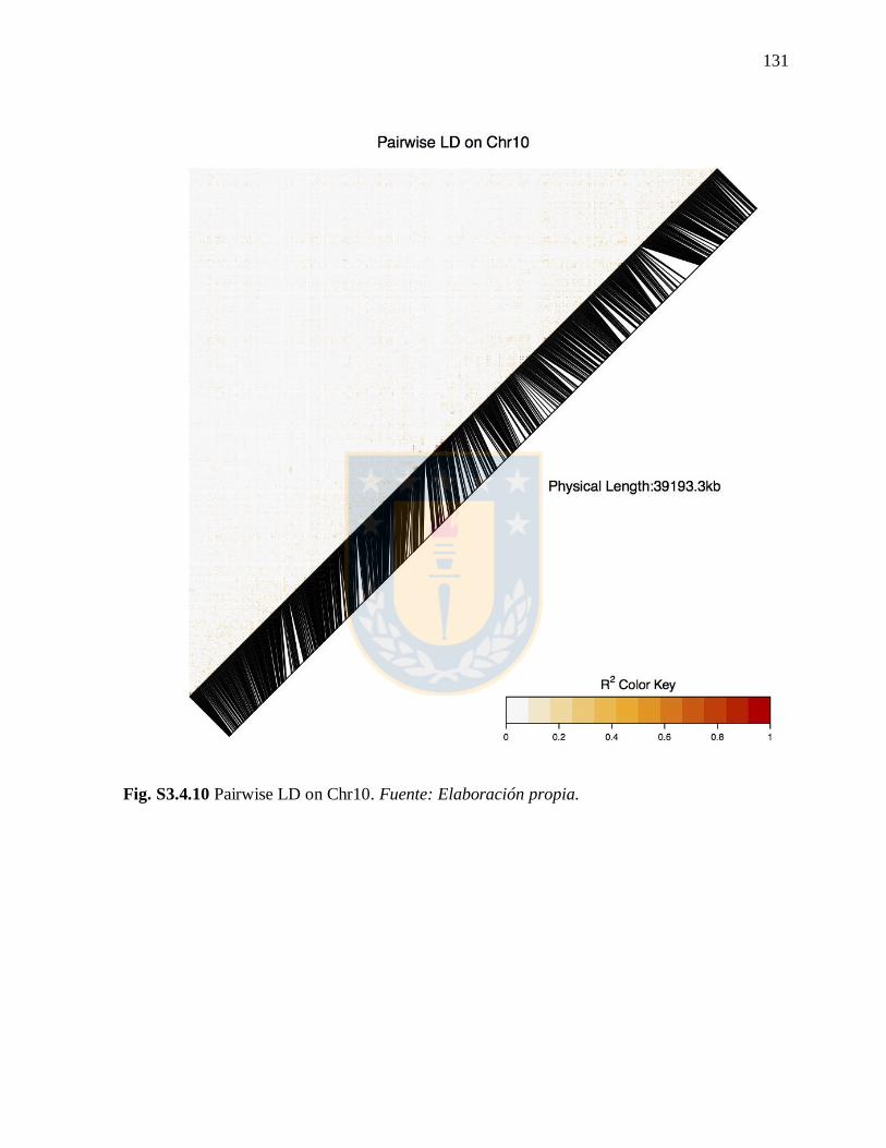
131
Fig. S3.4.10 Pairwise LD on Chr10. Fuente: Elaboración propia.

132
Fig. S3.4.11 Pairwise LD on Chr11. Fuente: Elaboración propia.

133
Fig. S3.5 Inbreeding values derived from shared SNP markers. Fuente: Elaboración propia.
0
20
40
60
0.6 0.8 1.0
Inbreeding
Fre
cuen
cy

134
Table S3.1 Evaluation of statistical models (GLUP, BLasso, Bayes B and Bayes C) by using
random sampling of 50 individuals with 2 folds and 10 replications for wood density and
volume. Fuente: Elaboración propia.
GBLUP BLasso Bayes B Bayes C
Trait/Statistics Mean (min-max) Mean (min-
max) Mean (min-max) Mean (min-max)
Wood density
Mean best 10% 3.5 (1.9-5.6) 3.5 (2.8-5.1) 3.8 (2.0-5.8) 3.8 (1.8-6.8)
MSE 16.5 (15.7-17.3) 6.4 (5.1-8.0) 13.3 (10.4-20.0) 11.8 (7.2-17.2)
Bias 1.2 (0.8-1.5) 1.0 (0.8-1.4) 0.91 (0.5-1.2) 1.0 (0.5-1.3)
Volume
Mean best 10% 34.6 (29.6-39.4) 34.87 (30.5-
38.3) 34.9(32.1-37.3) 33.7 (27.6-37.7)
MSE 108.6 (96.0-124.6) 63.8 (52.4-79.3) 237.0 (165.2-
313.9)
242.9 (202.4-
296.0)
Bias 1.1 (0.9-1.2) 1.44 (0.9-4.6) 1.1 (0.9-1.4) 1.1 (0.9-1.4)
135
DISCUSIÓN GENERAL
Los SNPs corresponden a diferencias bi, tri y tetra-alélicas en la secuencia de ADN en sitios
homólogos (Brookes 1999; Cho et al. 1999). Son el tipo de polimorfismos más abundante
dentro de los genomas y, teóricamente, se pueden encontrar en cualquier lugar de una
secuencia genómica (Rafalski 2002), hasta cercanos a algún locus de interés (Germano y Klein
1999; Picout-Newber et al. 1999). Hasta hace algunos años, su identificación era costosa,
difícil y requería de mucho tiempo de análisis. Sin embargo, gracias a las tecnologías NGS, el
descubrimiento de alto rendimiento de estos marcadores ha sido posible (van Tassel et al.
2008) y se ha vuelto más sencillo para especies que carecen de un genoma de referencia
(Bachlava et al. 2012) o con poca información genómica disponible (Davey et al. 2011; Kim
et al. 2016). Sin embargo, desafortunadamente, aún sigue siendo una tarea difícil para algunas
especies que poseen tamaños de genomas mayores y que contienen una alta cantidad de
secuencias repetidas (de Souza et al. 2016).
En el primer estudio presentado en este trabajo, se utilizó la tecnología de GBS para la
identificación de SNPs, de la cual no existen reportes previos para E. globulus en Chile. Si
bien se sabe que la secuenciación de todo el genoma por NGS es la herramienta ideal para la
identificación de estos marcadores, en presencia de un genoma de referencia, no es necesario
una mayor profundidad de secuenciación para fines de genotipificación. Por lo tanto, es
posible implementar este tipo de enfoque, basado en la reducción de la complejidad del
genoma por enzimas de restricción para el llamado de variantes (Gürcan et al. 2016). Hoy en
día, el uso de herramientas bioinformáticas ha generado diferentes flujos de trabajo (Bradbury
et al. 2014; Catchen et al. 2013) para extraer información sobre SNPs y genotipos desde una
gran cantidad de secuencias (Kagale et al. 2016; McCormack et al. 2013). Uno de los grandes
desafíos en GBS es el análisis de sus datos, el cual debe ser rápido y eficiente. Éste, considera
las secuencias brutas a partir la secuenciación, la separación de las muestras multiplexadas, el
filtrado de secuencias de baja calidad, el ordenamiento y alineamiento de secuencias y el
llamado de los SNPs (Scheben et al. 2017), además de la disponibilidad de un genoma de
referencia para la especie (Torkamaneh et al. 2016). En el estudio se presentó una alternativa
de flujo de trabajo utilizando diferentes herramientas de análisis de libre acceso, donde en
primer lugar, las librerías fueron secuenciadas en una sola dirección (single-read), siendo la
136
forma más simple de preparación de librerías para secuenciación Illumina. Sin embargo, sería
mejor considerar un tipo de secuenciación que permita leer desde ambos extremos de un
fragmento (paired-end), ya que genera una mayor calidad de lecturas para alineamientos en
contra de una referencia y una mejor identificación de zonas problemáticas dentro del genoma
como re-arreglos genómicos y elementos repetitivos (Hillier et al. 2008).
Dado que E. globulus es una especie que carece de genoma de referencia, se utilizó el genoma
de E. grandis para el mapeo de las librerías genómicas, obteniendo un alto número de SNPs
catalogados como monomórficos o diferencias nucleotídicas intra-especie. Sin embargo, el
alto número de marcadores monomórficos identificados puede atribuirse a productos de
errores en la secuenciación, principalmente en la etapa de amplificación e intensidad de
hibridación. Por otra parte, la mayoría de los SNPs se encontraban en regiones no codificantes,
ya que pueden llegar a ser tres veces más frecuentes que aquellos en zonas codificantes (Ching
et al. 2002).
Como se ha discutido anteriormente, el objetivo fue optimizar el proceso de identificación de
SNPs, pero en general las características genómicas, la complejidad de los genoma, el nivel de
heterozigosidad, la proporción de secuencias repetitivas y el nivel de polimorfismo, pueden
contribuir positiva o negativamente a estos desafíos (Nielsen et al. 2011; Scheben et al. 2017).
También se discutieron diferentes factores técnicos que podrían estar afectando el proceso de
identificación y que han sido analizados en otros estudios para su mejora como la calidad del
ADN, el grado de multiplexación de muestras secuenciadas (Poland et al. 2012), número de
lecturas obtenidas por muestra (He et al. 2014), el largo de las secuencias (Melo et al. 2016) y
errores de secuenciación como datos perdidos (Brouard et al. 2017). Por lo tanto, es necesario
seleccionar parámetros apropiados, tales como, la profundidad de cobertura requerida, la
calidad del mapeo de lectura o el grado de divergencia para un mapeo exitoso (Torkamaneh et
al. 2017). Por otra parte, se hace necesario una comparación entre diferentes flujos de trabajo,
principalmente para validar una mayor cantidad de SNPs comunes. Si bien se pensaba que es
muy difícil comparar las estadísticas resultantes de diferentes estudio, principalmente debido a
las metodologías utilizadas, técnicas de secuenciación, material base y que la detección de
SNPs es independientes en cada análisis (da Souza et al. 2016), se ha visto que es posible

137
identificar marcadores comunes bajo diferentes flujos de trabajo, utilizando diferentes
tecnologías de secuenciación (Mascher et al. 2013).
En este estudio, la utilización de GBS no fue enfocado en descubrir marcadores que pudieran
ser posteriormente utilizados como una matriz física de genotipificación (SNP-Chip), si no
más bien, para descubrir simultáneamente estos polimorfismos entre un grupo específico de
individuos y utilizar esta información para posteriores estudios de selección asistida. Para
poder evaluar el potencial de genotipificación de los SNPs descubiertos mediante GBS, un
análisis de agrupamiento de individuos, de acuerdo a su estructura genética, fue realizado para
la población “A” del estudio (datos no mostrados), donde los marcadores mostraron no ser
capaces de discriminar los grupos genéticos (familias) que se presentaban dentro de la
población (material suplementario MS1). Por lo tanto, considerando este resultado, el alto
costo de análisis, tiempo y recurso informático, se hizo necesaria la evaluación de una
siguiente alternativa que permitiera genotipificar de una manera rápida y fácil SNPs en E.
globulus.
En el segundo estudio presentado, se evaluó la capacidad de genotipificación del EUChip60k
para E. globulus, el primer chip generado a partir de la secuenciación de 12 especies diferentes
de Eucalyptus (Silva-Junior et al. 2015a). En el capítulo II se discutió la utilización de esta
herramienta como sistema de genotipificación clonal para la especie, pero es importante
agregar algunas de las capacidades técnicas que acompañan a la genotipificación por chip.
Aunque la tecnología se ha descrito como desfavorable para algunos enfoques de diversidad
genética (Ganal et al. 2012), o búsqueda de SNPs en genes específicos, son muchas más sus
ventajas las asociadas a su elección, principalmente por la gran cantidad de datos de salida,
información adicional relevante, el hecho de que no necesita una etapa de pre-procesamiento y
que además es mucho más rápido en análisis, eficiente y económico (Mason et al. 2017). Por
ejemplo, a partir de los análisis realizados, al comparar ambas tecnologías (GBS v/s Chip),
GBS permitió identificar un número previamente indeterminado de marcadores, que además
resultaron ser de baja calidad para posteriores análisis de genotipificación (Informe S4). Por su
parte, el EUChip60K entregó un alto número de SNPs de alta reproducibilidad, que pudieron

138
ser analizados simultáneamente y que fueron posteriormente utilizados para un análisis de
identidad.
Como se ha señalado anteriormente, los SNPs constituyen una importante fuente de MMs que
pueden tener variadas aplicaciones. Uno de ellos es la genotipificación de material genético,
tarea que hasta la fecha ha sido realizada satisfactoriamente por los marcadores SSR. En el
proceso de genotipado, para un buen análisis de marcadores desde un chip, uno de los puntos
críticos descritos ha sido siempre la calidad de ADN utilizado, por su influencia directa sobre
la calidad del llamado de cada variante (Chagné et al. 2015). Sin embargo, de acuerdo a los
resultados obtenidos en este estudio, este factor no afectaría la genotipificación. Dado lo
anterior, estrictos parámetros de calidad han sido ajustados para optimizar el proceso de
clustering de los marcadores (Myles et al. 2010; Verde et al. 2012), los que tampoco fueron
necesarios de calibrar cuando el llamado de SNPs desde el chip fue reportado. La presencia de
falsos positivos dentro del genotipado de SNPs por Chips, en muchos casos aumenta en
muestras de mala calidad, por lo que estrategias de depuración de aquellos SNPs que deben ser
excluidos para posteriores análisis se hace recurrente. Para mayor información, un completo
reporte sobre la generación de estas plataformas físicas de genotipado, posteriores análisis y
aplicaciones han sido descritos por Rasheed et al. (2017) y Nicolazzi et al. (2015). Ganal et al.
(2014) destacan además, que aún no está claro hasta qué punto la tecnología de GBS podría
reemplazar el genotipado por chips, considerando su falta de estandarización y dificultad para
comparar datos desde diferentes proyectos y laboratorios, mientras que los datos desde chips
resultan más comparables. Sin embargo, para otros autores, como Bajgain et al. (2016), los
estudios comparativos entre ambas tecnologías, demostraron que GBS puede ser un mejor
método de genotipado de SNPs, ya que es capaz de proporcionar una cobertura más amplia.
Sin embargo, el genotipado por SNP-chip requiere menos conocimiento computacional y
recursos para el procesamiento de datos.
Si bien los costos de genotipado por secuenciación y chips han ido reduciéndose con los años,
no es fácil predecir qué tecnología será más barata en un futuro próximo. Por ejemplo en
nuestros estudios, los costos asociados la genotipificación mediante GBS y chip tuvieron un
valor aproximado de 6 dólares por kilobase de SNPs, para ambas tecnologías, y de 60 dólares

139
por muestra, lo que grandes volúmenes, significaría considerables costos asociados solo al
sistema de genotipado.
Validada la estrategia de genotipado mediante el EUChip60k, esta plataforma fue utilizada
para genotipificar un nuevo set de muestras de E. globulus, donde un total de 12 K de SNPs
resultaron ser polimórficos y fueron utilizados para ajustar un modelo de predicción
genómico. La SG es una alternativa al mejoramiento asistido por marcadores que ha
revolucionado la genética animal (Hayes y Goddard 2010) y de plantas (Heslot et al. 2015)
para la predicción de valores genéticos. Ello ha generado en los últimos años grandes
expectativas para su aplicación en especies forestales, donde ha existido un aumento
significativo de trabajos publicados discutiendo la respuesta de los modelos de SG para
diferentes características de interés, comparando modelos estadísticos, métodos de validación
y densidad de marcadores, entre otros parámetros.
En el estudio presentado en el capítulo III, la capacidad predictiva de la SG, para estimar
valores genómicos para dos rasgos de interés (densidad de la madera y volumen del fuste), fue
evaluada bajo un modelo de validación cruzada, con una densidad media de SNPs y bajo
diferentes modelos estadísticos. En general, el modelo ajustado en este pequeño grupo de
clones de E. globulus reportó resultados bastante consistentes y prometedores, muy similares a
los ya publicados para especies de coníferas y eucaliptos por otros autores mencionados
anteriormente. Por ejemplo, no existieron diferencias en las habilidades de predicción de los
modelos GBLUP y aquellos basados en Bayes, lo que ha sido ampliamente validado para otras
especies, sugiriendo que, si bien la arquitectura genética de las características son complejas,
el modelo de GBLUP posee un buen ajuste, lo cual favorece su aplicación, principalmente
debido a la simplicidad de este modelo en comparación a aquellos no paramétricos y el bajo
consumo de análisis (Ratcliffe et al. 2015; Resende et al. 2017).
Entre los factores que más estarían influyendo en la habilidad de predicción de los modelos,
estaría el grado de relación genética capturada por los marcadores entre las poblaciones de
entrenamiento y validación, así como también el grado de DL favorecido por el tamaño
efectivo de la población. En el estudio, los individuos divididos entre población de

140
entrenamiento y validación fueron seleccionados aleatoriamente dentro del grupo total de
muestras, por lo tanto, si se aumentara el grado de relación entre ambas, las habilidades
predictivas podrían mejorar para ambas características ó disminuirían si la relación entre
ambas fuera inferior. En el estudio, no se presentaron altos grados de DL entre pares de
marcadores, resultado bastante similar a lo anteriormente propuesto por Silva-Junior y
Grattapaglia (2015b) para Eucalyptus. Por lo tanto, la capacidad de los modelos es atribuible
principalmente al grado de estrechez que existía en la población y que permitía estimar de
mejor manera los distintos grados de relaciones genéticas.
Dentro de las nuevas consideraciones para estudios en SG, se aconseja que los modelos deban
integrar relaciones más realistas y representativas de la población donde serán aplicados,
principalmente disminuyendo el grado de relación que existe entre la población de
entrenamiento y validación al momento ajustar la ecuación de predicción. Por ejemplo, en
Eucalyptus, los últimos reportes de SG han estimado la precisión de los modelos para clones y
familias de híbridos (E. grandis x E. urophylla), con pérdida no significativa de la habilidad
predictiva, en ausencia de relaciones entre los sets de entrenamiento y validación (Resende et
al. 2017). En el estudio presentado en este trabajo, al utilizar un set de muestras inferior a lo
reportado para estimación de valores genéticos por SG, se debe considerar en primer lugar, un
aumento en el número de individuos para reajustar las ecuaciones de predicción. Si bien
teóricamente la habilidad de predicción disminuiría en este nuevo set, creemos que la buena
representatividad de la población objetivo, dentro del primer grupo de entrenamiento utilizado
en el estudio, permitirá de igualmente perdidas no considerables de habilidad de predicción.
En el capítulo, adicionalmente se utilizó una densidad media de marcadores de 12 K para
ajustar el modelo. Comparado con estudios en Eucalyptus y Picea, se ha visto que con una
baja densidad de SNPs (~5.000), las habilidades predictivas son bastante estables,
independiente de la posición genómica de los marcadores (Müller et al. 2017; Lenz et al.
2017). Se debe considerar que la principal ventaja del uso de paneles de SNPs reducidos
podría ser la rentabilidad de la genotipificación, aunque se espera que a una mayor cantidad de
marcadores, estos tengan mejor capacidad de predicción a lo largo de diferentes generaciones,
principalmente debido a la recombinación y el DL (Solverg et al. 2008). GS se puede aplicar

141
de manera más eficiente en poblaciones más estructuradas donde las relaciones y el DL son
mayores, lo que requiere una menor cobertura del genoma para alcanzar una alta precisión de
predicción (Lenz et al. 2017).
La SG busca considerar la aplicabilidad de los modelos en futuras generaciones de
mejoramiento de diferentes especies, análisis que durante el último tiempo también han sido
reportado por Isik et al. (2016). En general los estudios plantean que, para estas estimaciones,
una buena estrategia para obtener mejores habilidades de predicción es considerar a los padres
dentro del set de entrenamiento donde el modelo estadístico es ajustado para la predicción; lo
mismo para el caso de híbridos que quieran ser predichos, donde sus padres debe ser
considerados para el ajuste. De acuerdo a lo propuesto por Tan et al. (2017a), los modelos
ajustados, exclusivamente con padres de especies puras, no permitirían buenas predicciones en
sus híbridos, lo que probablemente podría atribuirse a la divergencia genética entre las
especies y la falta consistente de DL entre las especies y sus híbridos. Actualmente, E.
globulus solo posee una generación de mejoramiento en Chile, sin embargo, esta
consideración debe ser evaluada para futuras proyecciones de nuevas cruzas, donde una nueva
generación de padres puede dar origen a nuevas poblaciones.
De acuerdo a lo descrito por Resende et al. (2012), los modelos genómicos resultan ser sitio-
específicos y su habilidad de predicción disminuye al ser evaluados en sets de validación
provenientes de sitios geográficamente más lejanos al sitio donde el modelo fue ajustado
(Gamal et al. 2015). Sin embargo, esto ha sido discutido y se ha visto que la precisión de los
modelos desarrollados con los datos desde un sitio, y validados en un segundo sitio, puede
seguir siendo alta o marginalmente inferior a las realizada en el mismo sitio. Estudios en
Piceas (Lenz et al. 2017; Beaulieu et al. 2014) indican que la interacción genotipo-ambiente
podría ser baja o con condiciones medio ambientales constantes, y que los modelos de SG
podrían ser aplicados en una amplia gama de sitios, sin necesidad de modelos independientes.
En éste estudio de SG, los clones utilizados están distribuidos en sitios muy cercanos, por lo
tanto, se espera que la capacidad de predicción de los modelos no se vea influenciada por el
efecto ambiental ó que su incidencia sea poco representativa de la variabilidad fenotípica que
pueda existir entre los sitios.

142
Finalmente, se debe discutir el hecho que los modelos de SG deberían considerar la
contribución no aditiva para las habilidades predictivas y así evaluar si la incorporación de
dominancia y/o epistasis mejora la efectividad de predecir valores genéticos de individuos o
familias. Esto ya ha sido evaluado en híbridos de Eucalyptus en donde el componente no
aditivo aumenta la eficiencia de los modelos de predicción para características de crecimiento
(Tan et al. 2017b). En el estudio de E. globulus, solo se consideró el efecto aditivo para las
predicciones genómicas, por lo tanto, este punto puede ser considerado para futuras
validaciones de precisión y habilidad de los modelos, posiblemente para estudios en híbridos.

143
MATERIAL SUPLEMENTARIO
MS1. Resultados del estudio de calidad de genotipificación de SNPs descubiertos mediantes
GBS, para una población clonal de E. globulus.
a) Clasificación de muestras de acuerdo al análisis exploratorio de PCs. Clusters
inferidos: Numero de grupos que fueron seleccionados de acuerdo a análisis de BIC.
Clusters originales: Familias originales a las que pertenece cada muestra.
Clu
ster
s ori
gin
ale
s Clusters inferidos
1 2 3 4 5
1 0 0 6 0 0
2 0 0 4 0 0
3 2 0 29 0 0
4 0 0 5 0 0
5 0 0 4 0 0
6 0 0 2 0 0
7 0 0 10 0 0
8 0 0 15 0 0
9 0 0 9 0 0
10 0 0 3 0 0
11 0 0 3 0 0
12 0 0 5 0 0
13 0 0 7 0 0
14 0 0 26 0 0
15 0 0 4 0 0
16 0 0 5 0 0
17 0 0 27 0 0
18 0 1 18 1 0
19 0 0 3 0 0
20 0 0 3 0 0
21 0 0 9 0 0

144
22 0 0 7 0 0
23 0 0 8 0 0
24 0 0 9 0 1
25 0 0 10 0 0
26 0 0 12 0 0
27 0 0 3 0 0
28 0 0 4 0 0
29 0 0 3 0 0
b) Plot 2D para clasificación de las muestras de acuerdo al k óptimo y el numero de
familias originales. Inf: Grupos inferidos a partir de análisis de BIC. Ori: Grupos
originales (familias). Las cajas en negro representan la cantidad de individuos
presentes en cada una de grupos inferidos de acuerdo a su origen familiar. El tamaño
de las cajas es proporcional al número de individuos agrupados.
c) Plot 2D. Análisis discriminante de componentes principales. Los numero representan
las familias a las que pertenecen las muestras. Los puntos presentan a las muestras de
cada familia. El gráfico DA eigenvalues muestra la distribución de la matriz de peso
para el análisis discriminante de PCs.
Po
bla
cio
nes o
rig
inale
s
Clusters inferidos

145

146
CONCLUSIONES GENERALES
Utilizando la tecnología de GBS, alrededor de 1.200 SNPs polimórficos, en cada una de las
poblaciones de clones de E. globulus estudiadas, pudieron ser descubiertos. Si bien estos
marcadores estaban distribuidos a lo largo del genoma, poseían un bajo nivel de polimorfismo
producto de la baja calidad de secuenciación obtenida por esta técnica y no fueron capaces de
estimar la estructura genéticas entre muestras analizadas.
La plataforma de genotipificación EUChip60K permitió identificar un set de SNPs con
capacidad de resolución de genotipos molculares a nivel intra-clonal y familiar. La
genotipificación mostró un alto porcentaje de marcadores correctamente asignados entre
duplicados de réplicas biológicas y técnicas. Por otra parte, la genotipificación mostró ser
independiente de la calidad del ADN utilizado.
Un set de 12 K de SNPs polimórficos identificados entre clones de E. globulus, utilizando el
EUChip60K, permitió estimar las relaciones genéticas entre individuos, con una distribución
continua y con modas cercanas a lo esperado para individuos no relacionados (0), medios
hermanos (0,25) y hermanos completos (0,50). Esta metodología representa una manera más
precisa las relaciones genéticas alcanzadas utilizando la información genealógica de la
población, donde se asume que los individuos dentro de un mismo grupo de parientes
comparten el mismo genoma. Sin embargo, utilizando esta densidad media de 12 K
marcadores, solo un bajo porcentaje de pares SNPs mostró estar en niveles de DL superior a
0,4 a nivel intra-cromosomal para los 11 cromosomas representados para Eucalyptus, lo que se
vió probablemente favorecido por la distancia entre ellos.
Los modelos de selección genómica, tuvieron correlaciones entre los valores genéticos
estimados y reales de 0,58 y 0,75, para densidad de la madera y volumen del fuste
respectivamente. Considerando que el análisis fue realizado en un set de muestras de solo 310
individuos provenientes de una sola generación de mejoramiento, por lo que debe ser validado
para un mayor número de individuos desde la población de mejoramiento.

147
BIBLIOGRAFÍA GENERAL
Bachlava E, Taylor CA, Tang S, Bowers JE, Mandel JR, Burke JM, Knapp SJ (2012) SNP
discovery and development of a high-density genotyping array for sunflower. PLoS
One 7:e29814.
Bajgain P, Rouse MN y Anderson JA (2016) Comparing genotyping-by-sequencing and single
nucleotide polymorphism chip genotyping for quantitative trait loci mapping in wheat.
Crop Science 56:232-248.
Beaulieu J, Doerksen TK, MacKay J, Rainville A, Bousquet J (2014) Genomic selection
accuracies within and between environments and small breeding groups in white
spruce. BMC Genomics 15:1048. doi:10.1186/1471-2164-15-1048
Bradbury PJ, Zhang Z, Kroon DE, Casstevens TM, Ramdoss Y, Buckler ES (2007) TASSEL:
Software for association mapping of complex traits in diverse samples. Bioinformatics.
23:2633–2635.
Brookes AJ (1999) The essence of SNPs. Gene 234:177-186
Brouard J S, Boyle B, Ibeagha-Awemu EM y Bissonnette N (2017) Low-depth genotyping-
by-sequencing (GBS) in a bovine population: strategies to maximize the selection of
high quality genotypes and the accuracy of imputation. BMC genetics 18: 32.
Brown GR, Bassoni DL, Gill GP, Fontana JR, Wheeler NC, Megraw RA, Davis MF, Sewell
MM, Tuskan GA, Neale DB (2003) Identification of quantitative trait loci influencing
wood property traits in loblolly pine (Pinus taeda L.). III. QTL Verification and
candidate gene mapping. Genetics 164:1537–1546.
Butcher P, Southerton S (2007) Marker-assisted selection in forestry species. In Marker-
Assisted Selection, Current Status and Future Perspectives in Crops, Livestock,
Forestry and Fish pp 283-305.
Calus MPL, Veerkamp RF (2007) Accuracy of breeding values when using and ignoring the
polygenic effect in genomic breeding value estimation with a marker density of one
SNP per cM. J Anim Breed Genet 124:362–368.
Catchen J, Hohenlohe PA, Bassham S, Amores A, Cresko WA (2013) Stacks: an analysis tool
set for population genomics. Mol Ecol. 22:3124–40.

148
Chagné D, Bianco L, Lawley C, Micheletti D, Jacobs JME (2015) Methods for the design,
implementation, and analysis of Illumina InfiniumTM SNP assays in plants. In: Plant
genotyping: methods and protocols. Springer, New York, pp 281–298.
Ching A, Caldwell KS, Jung M, Dolan M, Smith OS, Tingey S, Morgante M y Rafalski AJ
(2002) SNP frequency, haplotype structure and linkage disequilibrium in elite maize
inbred lines. BMC Genet 3:19–32.
Cho RJ, Mindrinos M, Richards DR (1999) Genome wide mapping with biallelic markers in
Arabidopsis thaliana. Nat Genet 23:203–207.
Corporación Nacional Forestal. (2013) Por un Chile forestal sustentable. Santiago, Chile. p 83.
Davey JW, Hohenlohe PA, Etter PD et al (2011) Genome-wide genetic marker discovery and
genotyping using next generation sequencing. Nat Rev Genet, 12:499–510.
de Souza LM, Toledo-Silva G, Cardoso-Silva CB, Da Silva CC, de Araujo Andreotti IA et al
(2016) Development of single nucleotide polymorphism markers in the large and
complex rubber tree genome using next-generation sequence data. Molecular breeding,
36:115.
Devey ME, Carson SD, Nolan MF, Matheson AC, Te Riini C, Hohepa J (2004) QTL
associations for density and diameter in Pinus radiata and the potential for marker-
aided selection. Theor Appl Genet 108:516–524.
Doughty RW (2000) The eucalyptus: a natural and commercial history of the gum tree.
Baltimore, Maryland
Eldridge KG, Davidson J, Harwood CE, van Wyk G (1993) Eucalypt domestication and
breeding. Clerendon Press, Oxford
El-Kassaby YA, Isik F, Whetten R (2014) Modern advances in tree breeding. In Challenges
and Opportunities for the World's Forests in the 21st Century. Springer, Netherlands,
pp 441-459
Elshire RJ, Glaubitz JC, Sun Q, Poland JA, Kawamoto K, Buckler ES, Mitchel SE (2011) A
robust, simple genotyping-by- sequencing (GBS) approach for high diversity species.
PLoS One 6:e19379
Gamal El-Dien O, Ratcliffe B, Klápšte J, Chen C, Porth I, El-Kassaby YA (2015) Prediction
accuracies for growth and wood attributes of interior spruce in space using genotyping-
by-sequencing. BMC Genomics 16:370.

149
Ganal MW, Polley A, Graner EM, Plieske J, Wieseke R, Luerssen H y Durstewitz G (2012)
Large SNP arrays for genotyping in crop plants. J Biosci 37:821–828.
Ganal MW, Wieseke R, Luerssen H, Durstewitz G, Graner EM, Plieske J y Polley A (2014)
High-throughput SNP profiling of genetic resources in crop plants using genotyping
arrays. In Genomics of Plant Genetic Resources. Springer, Netherlands, pp 113-130.
Grattapaglia D (2014) Breeding forest trees by genomic selection: current progress and the
way forward. In Genomics of plant genetic resources. Springer, Netherlands, pp 651–
682.
Grattapaglia D, Resende MDV (2011) Genomic selection in forest tree breeding. Tree Genet
Genomes 7:241–255.
Germano J, Klein AS (1999) Species-specific nuclear and chloroplast single nucleotide
polymorphisms to distinguish Picea glauca, P. mariana and P. rubens. Theor Appl
Genet 99:37–49.
González‐ Martínez SC, Krutovsky KV, Neale DB (2006) Forest‐ tree population genomics
and adaptive evolution. New Phytologist, 170(2), 227-238.
Gürcan K, Teber S, Ercisli S y Yilmaz KU (2016) Genotyping by Sequencing (GBS) in
Apricots and Genetic Diversity Assessment with GBS-Derived Single-Nucleotide
Polymorphisms (SNPs). Biochemical genetics, 54:854-885.
Habier D, Fernando RL, Dekkers JCM (2009) Genomic selection using low-density marker
panels. Genetics society of America 182:343-353.
Hamilton HP, Hansey CN, Whitty BR, Stoffel K, Massa AN, Van Deynze A, De Jong WS,
Douches DS, Buell CR (2011) Single nucleotide polymorphism discovery in elite north
american potato germplasm. BMC Genomics 12:302.
Hayes BJ, Bowman PJ, Chamberlain AJ, Goddard ME (2009) Invited review: Genomic
selection in dairy cattle: Progress and challenges. J. Dairy Sci. 92:433–443.
Hayes B, Goddard M (2010) Genome-wide association and genomic selection in animal
breeding. Genome 53:876–883. doi:10.1139/ G10-076.
He J, Zhao X, Laroche A, Lu ZX, Liu H y Li Z (2014) Genotyping-by-sequencing (GBS), an
ultimate marker-assisted selection (MAS) tool to accelerate plant breeding. Front Plant
Sci 5:484.
150
Heffner EL, Sorrell ME, Jannink JL (2009) Genomic selection for crop improvement. Crop
Sci. 49:1–12.
Heslot N, Jannink JL, Sorrells ME (2015). Perspectives for genomic selection applications and
research in plants. Crop Sci 55: 1–12.
Hillier LW, Marth GT, Quinlan AR, Dooling D, Fewell G, Barnett D, Fox P et al (2008)
Whole-genome sequencing and variant discovery in C. elegans. Nat Methods 5:183–
188.
Instituto Forestal (2014) Mejoramiento genético de Eucalyptos en Chile. Santiago, Chile. p
488.
Instituto Forestal (2016) Anuario Forestal. Boletín estadístico Nº 154. Santiago, Chile. p 171.
Ipinza R (2000) Modelo Básico de Mejora Genética. En: Domesticación y Mejora Genética de
Raulí y Roble. Editado por Roberto Ipinza, Braulio Gutiérrez y Verónica Emhart;
Editora e Imprenta Maval Ltda, pp 197-213.
Isik F (2014) Genomic selection in forest tree breeding: the concept and an outlook to the
future. New For. 45:379–401.
Isik F, Bartholomé J, Farjat A, Chancerel E, Raffin A, Sanchez L, Plomion C, Bouffier L
(2016) Genomic selection in maritime pine. Plant Sci 242:108–119.
Jehan T, Lakhanpaul S (2006) Single nucleotide polymorphism (SNP)–methods and
applications in plant genetics: a review.
Jones E, Chu WC, Ayele M, Ho J, Bruggeman E, Yourstone K, Rafalski A et al (2009).
Development of single nucleotide polymorphism (SNP) markers for use in commercial
maize (Zea mays L.) germplasm. Mol Breeding. 24:165–176
Kagale S, Koh C, Clarke WE, Bollina V, Parkin IA y Sharpe AG (2016) Analysis of
genotyping-by-sequencing (GBS) data. Plant Bioinformatics: Methods and Protocols
269-284.
Kim C, Guo H, Kong W, Chandnani R, Shuang LS y Paterson AH (2016) Application of
genotyping by sequencing technology to a variety of crop breeding programs. Plant Sci
242:14–22.
Lande R, Thompson R (1990) Efficiency of marker-assisted selection in the improvement of
quantitative traits. Genetics 124:743–756.

151
Lenz PR, Beaulieu J, Mansfield SD, Clément S, Desponts M, Bousquet J (2017) Factors
affecting the accuracy of genomic selection for growth and wood quality traits in an
advanced-breeding population of black spruce (Picea mariana). BMC genomics
18:335.
Mascher M, Wu S, Amand PS, Stein N, Poland J (2013) Application of Genotyping-by-
Sequencing on Semiconductor Sequencing Platforms: A Comparison of Genetic and
Reference-Based Marker Ordering in Barley. PLoS ONE 8:e76925.
Mason AS, Higgins EE, Snowdon RJ, Batley J, Stein A, Werner C y Parkin IA (2017) A user
guide to theBrassica60K Illumina Infinium™ SNP genotyping array. Theoretical and
Applied Genetics 1-13.
McCormack JE, Hird SM, Zellmer AJ, Carstens BC y Brumfield RT (2013) Applications of
next-generation sequencing to phylogeography and phylogenetics. Mol. Phylogenet.
Evol. 66:526–538.
Melo AT, Bartaula R y Hale I (2016) GBS-SNP-CROP: a reference-optional pipeline for SNP
discovery and plant germplasm characterization using variable length, paired-end
genotyping-by-sequencing data. BMC bioinformatics 17:29.
Meuwissen THE, Hayes BJ, Goddard ME (2001) Prediction of Total Genetic Value Using
Genome-Wide Dense Marker Maps. Genetics 157:1819–1829.
Misztal I (2011) FAQ for genomic selection. Editorial. J. Anim. Breed. Genet. 128:245–246.
Muranty H, Jorge V, Bastien C, Lepoittevin C, Bouffier L, Sanchez L (2014) Potential for
marker-assisted selection for forest tree breeding: lessons from 20 years of MAS in
crops, Tree Genet. Genomes 10:1491-1510.
Myles S, Chia JM, Hurwitz B et al (2010) Rapid genomic characterization of the genus
Vitis. PLoS One 5:e8219.
Müller BS, Neves LG, de Almeida Filho JE, Resende MF, Muñoz PR, dos Santos PE et al
(2017) Genomic prediction in contrast to a genome-wide association study in
explaining heritable variation of complex growth traits in breeding populations of
Eucalyptus. BMC genomics 18:524.

152
Neale DB, Savolainen O (2004) Association genetics of complex traits in conifers. Trends
Plant Sci 9:325–330.
Neale DB, Sewell MM, Brown GR (2002) Molecular dissection of the quantitative inheritance
of wood property traits in loblolly pine. Ann. For. Sci. 59:595–605.
Nelson JC, Wang S, Wu Y, Li X, Antony G, White FF, Yu J (2011) BMC Genomics. 12:352
Nicolazzi E L, Biffani S, Biscarini F, Orozco ter Wengel P, Caprera A, Nazzicari N y Stella A
(2015) Software solutions for the livestock genomics SNP array revolution. Animal
genetics 46:343-353.
Nielsen R, Paul JS, Albrechtsen A y Song YS (2011) Genotype and SNP calling from next-
generation sequencing data. Nat Rev Genet. 12:443–51.
Novaes E, Drost DR, Farmerie WG, Pappas JR GJ, Grattapaglia D, Sederoff RR, Kirst M
(2008) High-throughput gene and SNP discovery in Eucalyptus grandis, an
uncharacterized genome. BMC Genomics 9:312.
Ona T, Sonoda T, Ito K, Shibata M, Tamai Y, Kojima K, Ohshima J, Yokota S, Yoshizawa N
(2001) Investigation of relationships between cell and pulp properties in Eucalyptus by
examination of within-tree property variations. Wood Science and Technology 35:229-
243.
Picoult-Newberg L, Ideker TE, Pohl MG, Taylor SL, Donaldson MA, Nickerson DA, Boyce-
Jacino M (1999) Milling SNPs from EST databases. Genome Res 9:167–174.
Plomion C, Bastien C, Bogeat-Triboulot MB, Bouffier L, Déjardin A, Duplessis S et al (2016)
Forest tree genomics: 10 achievements from the past 10 years and future prospects.
Annals of forest science 73:77-103.
Poland JA y Rife TW (2012) Genotyping-by-sequencing for plant breeding and genetics. Plant
Genome 5:92–102.
Rafalski A (2002) Applications of single nucleotide polymorphisms in crop genetics. Curr
Opin Plant Biol 5:94–100.
Ramírez M, Rodríguez J, Balocchi C, Peredo M, Elissetche JP, Mendonça R, Valenzuela S
(2009) Chemical composition and wood anatomy of Eucalyptus globulus clones:
Variations and relationships with pulpability and handsheet properties. J. Wood Chem.
Tech 29:43–58.

153
Rasheed A, Hao Y, Xia X, Khan A, Xu Y, Varshney RK y He Z (2017) Crop Breeding Chips
and Genotyping Platforms: Progress, Challenges, and Perspectives. Molecular Plant,
10:047-1064.
Ratcliffe B, El-Dien OG, Klapste J, Porth I, Chen C, Jaquish B et al. (2015).A comparison of
genomic selection models across time in interior spruce (Picea engelmannii x glauca)
using unordered SNP imputation methods. Heredity 115: 547–555.
Raymond CA, Banham P, MacDonald AC (1998) Within tree variation and genetic control of
basic density, fibre length and coarseness in Eucalyptus regnans in Tasmania. Appita J
51:299–305.
Resende MFR, Muñoz P, Acosta JJ, Peter GF, Davis JM, Grattapaglia D, Resende MDV,
Kirst M (2012) Accelerating the domestication of trees using genomic selection:
accuracy of prediction models across ages and environments. New Phytol 193:617–
624.
Resende RT, Resende MDV, Silva FF, Azevedo CF, Takahashi EK, Silva-Junior OB,
Grattapaglia D (2017) Assessing the expected response to genomic selection of
individuals and families in Eucalyptus breeding with an additive-dominant model.
Heredity 119:245.
Scheben A, Batley J y Edwards D (2017) Genotyping by sequencing approaches to
characterise crop genomes: choosing the right tool for the right application. Plant
biotechnology journal 15:149-161.
Sewell MM, Neale DB (2000) Mapping quantitative traits in forest trees. In Molecular biology
of woody plants Dordrecht, Netherlands, Kluwer, Vol. 1, pp 407–423.
Silva-Junior OB, Faria DA, Grattapaglia D (2015a) A flexible multi- species genome-wide
60K SNP chip developed from pooled resequencing of 240 Eucalyptus tree genomes
across 12 species. New Phytol 206:1527–1540. doi:10.1111/nph.13322.
Silva-Junior OB, Grattapaglia D (2015b) Genome-wide patterns of recombination, linkage
disequilibrium and nucleotide diversity from pooled resequencing and single
nucleotide polymorphism genotyping unlock the evolutionary history of Eucalyptus
grandis. New Phytol 208:830–845. doi:10.1111/nph.13505.

154
Solberg TR, Sonesson AK, Woolliams JA, Meuwissen THE (2008) Genomic selection using
different marker types and densities. Journal of animal science 86: 2447-2454.
Strauss S, Lande R, Namkoong G (1992) Limitations of molecular-marker-aided selection in
forest tree breeding. Can J For Res 22:1051–1061.
Tan B, Grattapaglia D, Martins GS, Ferreira KZ, Sundberg B, Ingvarsson PK (2017a)
Evaluating the accuracy of genomic prediction of growth and wood traits in two
Eucalyptus species and their F 1 hybrids. BMC plant biology, 17(1), 110.
Tan B, Grattapaglia D, Wu HX, Ingvarsson K (2017b) Genomic prediction reveals significant
non-additive effects for growth in hybrid Eucalyptus. bioRxiv 178160.
Thomson MJ, Zhao K, Wright M, McNally KL, Rey J, Tung CW, Reynolds A et al (2012)
High-throughput single nucleotide polymorphism genotyping for breeding applications
in rice using the BeadXpress platform. Mol Breeding 29:875–886.
Thumma RF, Nolan MF, Evans R, Moran GF (2005) Polymorphisms in cinnamoyl CoA
reductase (CCR) are associated with variation in microfibril angle in Eucalyptus spp.
Genetics 171:1257–1265.
Trebbi T, Maccaferri M, De Heer P, Sørensen A, Giuliani S, Salvi S, Sanguineti MC, Massi A,
Gerard van der Vossen EA, Tuberosa R (2011) High-throughput SNP discovery and
genotyping in durum wheat (Triticum durum Desf.). Theor Appl Genet 123:555–569.
Torkamaneh D, Laroche J y Belzile F (2016) Genome-wide SNP calling from genotyping by
sequencing (GBS) data: a comparison of seven pipelines and two sequencing
technologies. PloS one 11:e0161333.
Torkamaneh D, Laroche J, Bastien M, Abed A y Belzile F (2017) Fast-GBS: a new pipeline
for the efficient and highly accurate calling of SNPs from genotyping-by-sequencing
data. BMC bioinformatics 18:5.
Vallejos J, Badilla Y, Picado F, Murillo O (2010) Metodología para la selección e
incorporación de árboles plus en programas de mejoramiento genético forestal.
Agronomía Costarricense 34:105-119.
van Tassell CP, Smith TPL, Matukumalli LK et al (2008) SNP discovery and allele frequency
estimation by deep sequencing of reduced representation libraries. Nat Methods,
5:247–52.

155
Verde I, Bassil N, Scalabrin S, Gilmore B, Lawley CT, Gasic K et al (2012) Development and
evaluation of a 9K SNP array for peach by internationally coordinated SNP detection
and validation in breeding germplasm. Plos one 7:e35668.
White TL, Adams WT, Neale DB (2007). Forest genetics. CABI Publishing CAB
International, Cambridge.
Wimmer R, Downes GM, Evans R, Rasmussen G, French J (2002) Direct effects of wood
characteristics on pulp and paper handsheet properties of Eucalyptus globulus.
Holzforschung 56:244–252.
Wong C, Bernardo R (2008) Genome-wide selection in oil palm: increasing selection gain per
unit time and cost with small populations. TAG Theoretical and Applied Genetics
116:815-824.
You FM, Huo N, Deal KR, Gu YQ, Luo MC, McGuire PE, Dvorak J, Anderson OD (2011)
Annotation-based genome- wide SNP discovery in the large and complex Aegilops
tauschii genome using next-generation sequencing without a reference genome
sequence. BMC Genomics 12:59.
Zapata-Valenzuela J, Hasbun R (2011) Mejoramiento genético forestal acelerado mediante
selección genómica. Bosque (Valdivia) 32:209–213.
Zhao Y, Gowda M, Liu W, Würschum T, Maurer HP, Longin FH, Ranc N, Reif JC (2012)
Accuracy of genomic selection in European maize elite breeding populations. Theor.
Appl. Genet. 124: 769-776.


![HabilidadesFP1.pps [Modo de compatibilidad]qinnova.uned.es/archivos_publicos/webex_actividades/4815/... · Lecturas complementarias ... la predicción de resultados y la selección](https://img.pdfslide.tips/doc/110x75/5ba6e5ad09d3f22f1b8c40d8/modo-de-compatibilidadqinnovaunedesarchivospublicoswebexactividades4815.jpg)