Embed Size (px)
Citation preview
Monotonicity in Asset Returns: New Tests with Applications to
the Term Structure, the CAPM and Portfolio Sorts�
Andrew J. Patton
University of Oxford
Allan Timmermann
University of California San Diego
30 April 2009
Abstract
Many theories in �nance imply monotonic patterns in expected returns and other �nancial
variables: The liquidity preference hypothesis predicts higher expected returns for bonds with
longer times to maturity; the CAPM implies higher expected returns for stocks with higher
betas; and standard asset pricing models imply that the pricing kernel is declining in market
returns. The full set of implications of monotonicity is generally not exploited in empirical
work, however. This paper proposes new and simple ways to test for monotonicity in �nancial
variables and compares the proposed tests with extant alternatives such as t-tests, Bonferroni
bounds and multivariate inequality tests through empirical applications and simulations.
JEL Codes: G12, G14
�We thank Susan Christo¤ersen, Erik Kole, Robert Kosowski, Jun Liu, Igor Makarov, Ross Valkanov, Simon van
Norden, Michela Verardo and seminar participants at HEC Montreal and the Adam Smith Asset Pricing workshop
at Imperial College London for helpful comments and suggestions. This is a substantially revised version of the paper
titled �Portfolio sorts and tests of cross-sectional patterns in expected returns.�Patton: Department of Economics
and Oxford-Man Institute of Quantitative Finance, University of Oxford, Manor Road, Oxford OX1 3UQ, United
Kingdom. Email: [email protected]. Timmermann: Rady School of Management and Department
of Economics, University of California, San Diego, 9500 Gilman Drive, La Jolla, CA 92093-0553, USA. Email:
1 Introduction
Finance contains many examples of theories which imply that expected returns should be monoton-
ically decreasing or monotonically increasing in securities�risk or liquidity characteristics. For ex-
ample, under the liquidity preference hypothesis, expected returns on treasury securities should
increase monotonically with their time to maturity; the CAPM implies a monotonically increasing
pattern in the expected return of stocks ranked by their market betas. Another fundamental impli-
cation of �nance theory is that the pricing kernel should be monotonically decreasing in investors�
ranking of future states as measured, e.g., by market returns.
The full set of implications of such monotonic patterns is generally not explored, however,
in empirical analysis. For example, when testing the CAPM, it is conventional practice to form
portfolios of stocks ranked by their beta estimates. A t-test may then be used to consider the mean
return di¤erential between the portfolios with the highest and lowest betas. Yet comparing only
the average returns on the top and bottom portfolios does not provide a su¢ cient way to test for
a monotonic relation between expected returns and betas. As an illustration, Figure 1 presents
average monthly returns on stocks sorted into deciles according to their estimated betas. The mean
return on the high-beta stocks exceeds that of the low-beta stocks, but a t�test on the top-minus-
bottom return di¤erential comes out insigni�cant. A test that only considers the return di¤erence
between the top and bottom ranked securities does not utilize the observation from Figure 1 that
none of the declining segments�which go against the CAPM�appears to be particularly large, so
the question arises whether the CAPM is in fact refuted by this evidence.
As a second illustration, Figure 2 shows the term premia on T-bills with a maturity between 2
and 11 months. Clearly the overall pattern in the term premium is increasing, and this is con�rmed
by a t�test on the mean di¤erential between the 11- and 2-month bills which comes out signi�cant.
However, there are also segments where the term premium appears to be negative�particularly
between the 9 and 10-month bills�so the question here is whether there are su¢ ciently many,
and su¢ ciently large, negative segments to imply a rejection of the liquidity preference hypothesis.
Only a test that simultaneously considers the mean returns across all maturities can answer this.
This paper proposes new ways to test for monotonicity in the expected returns of securities
sorted by characteristics which theory predicts should earn a systematic premium. Our tests are
nonparametric and easy to implement via bootstrap methods. Thus they do not require specifying
1

the functional form (e.g. linearity) relating the sorting variables to expected returns. This is
important because for many economic models the underlying hypothesis is only that expected
returns should rise or decline monotonically in one or more security characteristics that proxy for
risk exposures or liquidity.
In common with a conventional one-sided t�test, our monotonic relation (MR) test holds that
expected returns are identical or weakly declining under the null, while under the alternative we
maintain a monotonically increasing relation. (Testing for a monotonic decreasing relation can
of course be accomplished by simply re-ordering the assets.) Thus a rejection of the null of no
relationship in favor of the hypothesized relationship (i.e. a �nding of �statistical signi�cance�)
represents a strong empirical endorsement of the theory. We also develop separate tests based on
the sum of �up�and �down�moves. These combine information on both the number and magnitude
of deviations from a �at pattern and so can help determine the direction of deviations in support
of or against the theory.
The converse approach of maintaining a monotonically increasing relation under the null versus
no such relationship under the alternative has been developed by Wolak (1987, 1989) and was also
adopted by Fama (1984) in the context of a Bonferroni bound test to summarize the outcome
of several t�tests. Depending on the research question and the economic framework, one may
prefer to entertain the presence of a monotonic relationship under the null or under the alternative
hypothesis. Richardson et al. (1992), for example, used the Wolak test to see if there was evidence
against an upward-sloping term structure of interest rates, as predicted by the liquidity preference
hypothesis.
Since the MR and Wolak tests use di¤erent ways to test the theory, outcomes from such tests are
not directly comparable. One drawback of entertaining the hypothesized monotonic relationship
under the null is that a con�rmation of a theory from a failure to reject the null may simply be due
to limited power for the test (due to a short time series of data, or due to noisy data, for example).
This turns out to be empirically important as the Wolak test sometimes fails to reject the null in
cases where the t-test and the MR test are able to di¤erentiate between theories that �nd support
in the data and those that do not. Conversely, in cases where the MR test has weak power, it may
fail to reject the null�and thus fail to support the theory�even for expected return patterns that
appear to be monotonic.
Empirically, our tests reveal many interesting �ndings. For the CAPM example shown in Figure
2

1, the MR test strongly rejects the null in favor of a monotonically increasing relationship between
portfolio betas and expected returns. Consistent with this, the Bonferroni bound and Wolak tests
fail to reject the null that expected returns increase in betas. Turning to the term structure example
in Figure 2, the MR, Bonferroni and Wolak tests all fail to �nd evidence in support of the liquidity
preference hypothesis as the term premia do not appear to be monotonically increasing in the
maturity. Moreover, when applied to a range of portfolio sorts considered in the empirical �nance
literature, we �nd many examples where the di¤erence in average returns between the top and
bottom portfolios is highly signi�cant, but the pattern in average returns across multiple portfolios
is non-monotonic. This holds, for example, for decile portfolios sorted on short-term reversal,
momentum or �rm size.
Our tests are not restricted to monotonic patterns in the expected returns on securities sorted on
one or more variables and can be generalized to test for monotonic patterns in risk-adjusted returns
or in the factor loadings emerging from asset pricing models. They can also be adopted to test
for piece-wise monotonic patterns, as in the case of the U-shaped relationship between fee waivers
and mutual fund performance reported by Christo¤ersen (2001) or the U-shaped pricing kernels
considered by Bakshi et al. (2009). Finally, using methods for converting conditional moments into
unconditional ones along the lines of Boudoukh et al. (1999), we show that the approach can be
used to conduct conditional tests of monotonicity.
The outline of the paper is as follows. Section 2 describes our new approach to testing for
monotonic patterns in expected returns on securities ranked by one or more variables and compares
it with extant methods. Section 3 uses the various methodologies to analyze a range of return series
from the empirical �nance literature. Section 4 uses Monte Carlo simulations to shed light on the
behavior of the tests under a set of controlled experiments. Finally, Section 5 concludes.
2 Testing Monotonicity
This section �rst provides some examples from �nance to motivate monotonicity tests. We next
introduce the monotonic relationship test and compare it with extant alternatives such as a student
t�test based on top-minus-bottom return di¤erentials, the multivariate inequality test proposed
by Wolak (1989) and the Bonferroni bound.
3

2.1 Monotonicity Tests in Finance
One of the most basic implications of �nancial theory is that the pricing kernel should be monoton-
ically decreasing in investors�ordering of future states (Shive and Shumway (2009)). In empirical
work, this implication is typically tested by studying pricing kernels as a function of market returns.
Using options data, Jackwerth (2000) �nds that this prediction is supported by the data prior to
the October 1987 crash, where risk aversion functions were monotonically declining. However, it
appears to no longer hold in post-crash data. Rosenberg and Engle (2002) also �nd evidence of
a region with increasing marginal utility for small positive returns. These papers do not formally
test monotonicity of the pricing kernel, however.
The practice of looking for monotonic patterns in expected returns on portfolios of stocks sorted
by observables such as �rm size or book-to-market ratio can be motivated by the fact that, although
such variables are clearly not risk factors themselves, they may serve as proxies for unobserved risk
exposures. For example, Berk, Green and Naik (1999) develop a model of �rms�optimal investment
choices where expected returns depend on a single risk factor. Estimating the true betas with regard
to this risk factor requires knowing the covariance of each investment project in addition to the
entire stock of ongoing projects�a task that is likely to prove infeasible. However, expected returns
can be re-written in terms of observable variables such as the book-to-market ratio and size which
become su¢ cient statistics for the risk of existing assets. Hence expected returns on portfolios
of stocks sorted on these variables should be monotonically increasing in book-to-market value
and monotonically decreasing in size. Similar conclusions are drawn from the asset pricing model
developed by Carlson et al. (2004).
As a second illustration, in a model of momentum e¤ects where growth rate risk rises with
growth rates and has a positive price, Johnson (2002) shows that expected returns should be
monotonically increasing in securities�past returns and uses decile portfolios to study this impli-
cation.
If factor loadings on risk factors are either observed or possible to estimate without much error,
then tests based on the linear asset pricing model may be preferable on e¢ ciency grounds. However,
in situations where the nature (functional form) of the relationship between expected returns and
some observable variable used to rank or sort is unknown, the linear regression approach may be
subject to misspeci�cation biases. Hence there is inherently a trade-o¤ between the e¢ ciency of
4

regression models that assume linearity, but make use of the full data, versus tests based on portfolio
sorts that do not rely on this assumption. Tests of monotonicity between expected portfolio returns
and observable stock characteristics such as book-to-market value or size o¤er a fairly robust way to
test asset pricing models, although they should be viewed as joint tests of the hypothesis that the
sorting variable proxies for exposure to the unobserved risk factor and the validity of the underlying
asset pricing model.
2.2 Monotonicity and Inequality Tests
The problem of testing for the presence or absence of a monotonic pattern in expected returns can
be transformed into tests of inequality restrictions on estimated parameters. Consider a simple
example where decile portfolios have been formed by sorting stocks based on their past estimated
market betas. Letting r1;t; ::::; r10;t be the associated returns on the decile portfolios listed in
ascending order, the CAPM implies that the expected returns on these portfolios are increasing:
E [r10;t] > E [r9;t] > � � � > E [r1;t] : (1)
If we de�ne �i � E [ri;t]� E [ri�1;t] ; for i = 2; :::; 10; this implication can be re-written as
�i > 0 for i = 2; :::; 10: (2)
Alternatively, consider a test of the liquidity premium hypothesis (LPH), as in Richardson, et al.
(1992) and Boudoukh, et al. (1999). If we de�ne the term premium as Ehr(� i)t � r(1)t
i; where r(� i)t
is the one-period return on a bond with maturity � i; the simplest form of the LPH implies
Ehr(� i)t � r(1)t
i> E
hr(�j)t � r(1)t
ifor all � i � � j : (3)
That is, term premia are increasing with maturity. If we de�ne�i � Ehr(� i)t � r(1)t
i�E
hr(� i�1)t � r(1)t
i,
then this prediction can be re-written as
�i > 0 for i = 2; :::; N: (4)
We next propose a new and simple non-parametric approach that tests directly for the presence
of a monotonic relation between expected returns and the underlying sorting variable(s) but does
not otherwise require that this relationship be speci�ed or known. This can be a great advantage
in situations where standard distributions are unreliable guides for the test statistics, di¢ cult to
5
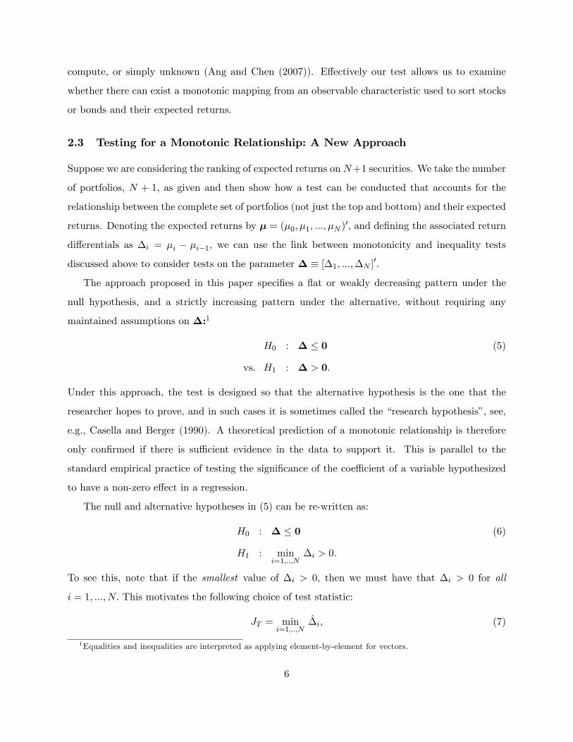
compute, or simply unknown (Ang and Chen (2007)). E¤ectively our test allows us to examine
whether there can exist a monotonic mapping from an observable characteristic used to sort stocks
or bonds and their expected returns.
2.3 Testing for a Monotonic Relationship: A New Approach
Suppose we are considering the ranking of expected returns on N+1 securities. We take the number
of portfolios, N + 1, as given and then show how a test can be conducted that accounts for the
relationship between the complete set of portfolios (not just the top and bottom) and their expected
returns. Denoting the expected returns by � = (�0; �1; :::; �N )0, and de�ning the associated return
di¤erentials as �i = �i � �i�1, we can use the link between monotonicity and inequality tests
discussed above to consider tests on the parameter � � [�1; :::;�N ]0.
The approach proposed in this paper speci�es a �at or weakly decreasing pattern under the
null hypothesis, and a strictly increasing pattern under the alternative, without requiring any
maintained assumptions on �:1
H0 : � � 0 (5)
vs. H1 : � > 0:
Under this approach, the test is designed so that the alternative hypothesis is the one that the
researcher hopes to prove, and in such cases it is sometimes called the �research hypothesis�, see,
e.g., Casella and Berger (1990). A theoretical prediction of a monotonic relationship is therefore
only con�rmed if there is su¢ cient evidence in the data to support it. This is parallel to the
standard empirical practice of testing the signi�cance of the coe¢ cient of a variable hypothesized
to have a non-zero e¤ect in a regression.
The null and alternative hypotheses in (5) can be re-written as:
H0 : � � 0 (6)
H1 : mini=1;::;N
�i > 0:
To see this, note that if the smallest value of �i > 0, then we must have that �i > 0 for all
i = 1; :::; N: This motivates the following choice of test statistic:
JT = mini=1;::;N
�̂i; (7)
1Equalities and inequalities are interpreted as applying element-by-element for vectors.
6

where �̂i is based on the sample analogs �̂i = �̂i � �̂i�1; �̂i � 1T
PTt=1 rit and fritgTt=1 is the time
series of returns on the ith security.
In Section 2.5 we discuss how we obtain appropriate critical values for this test statistic using a
bootstrap procedure. We shall refer to the tests associated with hypotheses such as those in (6) as
Monotonic Relationship (MR) tests. Testing that expected returns are monotonically decreasing
can be done simply by reordering the assets.
Note that in (7) we consider all �adjacent�pairs of security returns, while we could also consider
all possible pairwise comparisons, E [ri;t] � E [rj;t] for all i > j: The latter approach increases the
number of parameter constraints, and the size of the vector �, from N to N (N + 1) =2. The
adjacent pairs are su¢ cient for monotonicity to hold, but it is possible that considering all possible
comparisons leads to empirical gains. We compare the adjacent pairs test to the �all pairs�test in
our empirical analysis and Monte Carlo simulations. With the parameter � suitably modi�ed, the
theory presented below holds in both cases.
2.3.1 Diagnostic Tests for Monotonicity
The proposed MR test for monotonicity is useful for detecting the presence or absence of a
monotonic relationship between expected returns and some economic variable. However researchers
may also be interested in other aspects of this relationship, and so we propose two statistics that
provide further information. Suppose the MR test fails to reject the null in favor of a monotonically
increasing relationship, yet visual inspection suggests that the relationship is �mostly�increasing.
A useful test, then, would be one that determines whether the negatively-sloped parts of the pat-
tern are signi�cantly di¤erent from zero, which may help explain why the MR test does not reject
the null. To that end, consider the following null and alternative:
H0 : � = 0
vs. H�1 :
NXi=1
j�ij1 f�i < 0g ;
where the indicator 1 f�i < 0g is one if �i < 0, and otherwise is zero. Here the null is a �at
pattern (no relationship) and the alternative is that at least some parts of the pattern are strictly
negative. By summing over all negative deviations, this statistic accounts for both the frequency
7
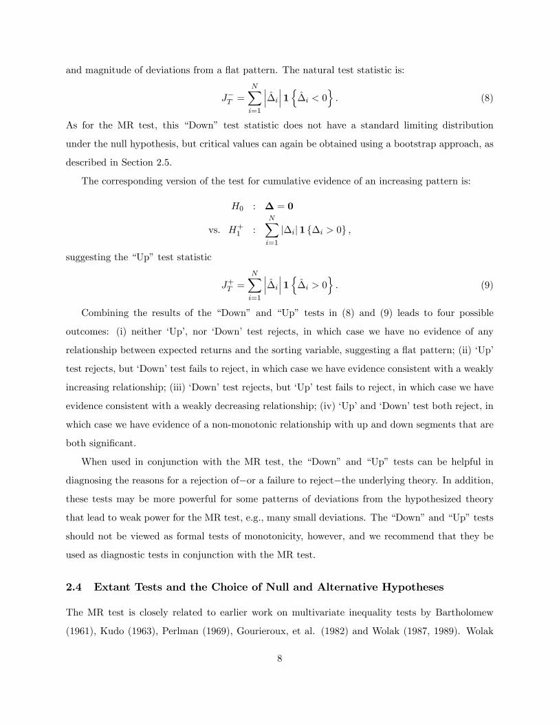
and magnitude of deviations from a �at pattern. The natural test statistic is:
J�T =NXi=1
����̂i���1n�̂i < 0o : (8)
As for the MR test, this �Down� test statistic does not have a standard limiting distribution
under the null hypothesis, but critical values can again be obtained using a bootstrap approach, as
described in Section 2.5.
The corresponding version of the test for cumulative evidence of an increasing pattern is:
H0 : � = 0
vs. H+1 :
NXi=1
j�ij1 f�i > 0g ;
suggesting the �Up�test statistic
J+T =
NXi=1
����̂i���1n�̂i > 0o : (9)
Combining the results of the �Down� and �Up� tests in (8) and (9) leads to four possible
outcomes: (i) neither �Up�, nor �Down� test rejects, in which case we have no evidence of any
relationship between expected returns and the sorting variable, suggesting a �at pattern; (ii) �Up�
test rejects, but �Down�test fails to reject, in which case we have evidence consistent with a weakly
increasing relationship; (iii) �Down�test rejects, but �Up�test fails to reject, in which case we have
evidence consistent with a weakly decreasing relationship; (iv) �Up�and �Down�test both reject, in
which case we have evidence of a non-monotonic relationship with up and down segments that are
both signi�cant.
When used in conjunction with the MR test, the �Down� and �Up� tests can be helpful in
diagnosing the reasons for a rejection of�or a failure to reject�the underlying theory. In addition,
these tests may be more powerful for some patterns of deviations from the hypothesized theory
that lead to weak power for the MR test, e.g., many small deviations. The �Down�and �Up�tests
should not be viewed as formal tests of monotonicity, however, and we recommend that they be
used as diagnostic tests in conjunction with the MR test.
2.4 Extant Tests and the Choice of Null and Alternative Hypotheses
The MR test is closely related to earlier work on multivariate inequality tests by Bartholomew
(1961), Kudo (1963), Perlman (1969), Gourieroux, et al. (1982) and Wolak (1987, 1989). Wolak
8
(1989) proposed a test that entertains (weak) monotonicity under the null hypothesis, and speci�es
the alternative as non-monotonic:
H0 : � � 0 (10)
vs. H1 : � unrestricted.
Here the theoretical prediction of monotonicity is contained in the null hypothesis and is only
rejected if the data contain su¢ cient evidence against it. The test statistic in this approach is
based on a comparison of an unconstrained estimate of � with an estimate obtained by imposing
weak monotonicity. Wolak (1987, 1989) shows that these test statistics have a distribution under
the null that is a weighted sum of chi-squared variables,PNi=1 !(N; i)�
2(i), where !(N; i) are the
weights and �2(i) is a chi-squared variable with i degrees of freedom. Critical values are generally
not known in closed form, but a set of approximate values can be calculated through Monte Carlo
simulation. This procedure is computationally intensive and di¢ cult to implement in the presence of
large numbers of inequalities. As a result, the test has only found limited use in �nance. Richardson
et al. (1992) applied the method in Wolak (1989) to test for monotonicity of the term premium,
and in our empirical work below we present the results of Wolak�s test for comparison.
It is worth noting an important di¤erence between the MR approach in equation (6) and that of
Wolak (1989) in equation (10). In Wolak�s framework, the null hypothesis is that there is a weakly
monotonic relationship between expected returns and the sorting variable, while the alternative
hypothesis contains the case of no such monotonic relationship. Depending on the research question
and the economic framework, one may prefer to entertain the presence of a monotonic relationship
under the null or under the alternative. One potential drawback of entertaining the hypothesized
monotonic relationship under the null is that limited power (due to a short time series of data, or
due to noisy data) will make it di¢ cult to reject the null hypothesis and thus di¢ cult to have much
con�dence in a con�rmation of a theory from a failure to reject the null.2 The MR approach, on
the other hand, contains the monotonic relationship under the alternative, and thus a rejection of
the null of no relationship in favor of the hypothesized relationship represents a strong empirical
endorsement of the theory. Conversely, in cases where the MR test has weak power, it may fail
to reject the null and so incorrectly fail to support the theory entertained under the alternative
2Furthermore, the null equation (10) includes the case of no relationship (when � = 0) and so a failure to reject
the null could actually be the result of the absence of a relationship between expected returns and the sorting variable.
9
hypothesis. In such cases the �Up� and �Down� tests come in conveniently as they can help to
diagnose if the problem is indeed lack of power.
Since the setup of the null and alternative hypothesis under the MR test in equation (5) is the
mirror image of that under the Wolak test in (10), one cannot draw universally valid conclusions
about which approach is �best�. Rather, which test to use depends on the research question at hand.
The MR test is more appropriate to use when the relevant question is �Does the data support the
theory?�Conversely, the Wolak setup is more appropriate for a researcher interested in �nding out
if there is signi�cant evidence in the data against some theory. In cases where this distinction is not
clear, one could even consider inspecting both types of tests. There is strong support for the theory
if the MR test rejects while the Wolak test fails to reject. Conversely, if the Wolak test rejects while
the MR test fails to reject, this constitutes strong evidence against theory. Cases where both tests
fail to reject constitute weak con�rmation of the theory and could be due to the MR test having
weak power. Finally, if both tests reject, they disagree about the evidence. We should note that
we do not �nd a single case with this latter outcome in any of our empirical tests.
The MR test has greater apparent similarity to the setup of the multivariate one-sided tests
considered by Bartholomew (1961), Kudo (1963), Perlman (1969), Gourieroux, et al. (1982) and
labeled �EI�in Wolak (1989):
H0 : � = 0
vs. H1 : � � 0, (11)
with at least one inequality strict, under the maintained hypothesis Hm :� � 0: The test statistic
in this approach is based purely on an estimate of� obtained by imposing the maintained assump-
tion.3 The main drawback of this framework, if one wishes to test for a monotonic relationship,
is that if the true relationship is non-monotonic, then the behavior of the test is unknown, as the
maintained hypothesis is then violated. In a Monte Carlo study of this test (available upon request)
we found that it performed well when the maintained hypothesis was satis�ed. However when this
hypothesis is violated the �nite-sample size of the test tends to be very high, likely due to the fact
3Kudo characterized the weights analytically in cases with up to four constraints under the assumption that the
covariance matrix of the parameter estimator is known; Gourieroux et al. (1982) proposed simulation methods to
compute critical values when the covariance matrix is unknown; and Kodde and Palm (1986) derived lower and upper
bounds on the critical values for the test which avoids the need for simulations.
10
that this test is not designed to work when the maintained hypothesis of weak monotonicity is
violated. This leads the test to overreject and so we do not consider this test further here.
Lastly, a naïve approach to testing the hypotheses in equation (10) would be to conduct a set
of pair-wise t�tests to see if �i is positive for each i = 1; ::; N . Unfortunately, it is not clear how to
summarize information from these N tests into a single number since the test statistics are likely
to be correlated and their joint distribution is unknown. To deal with this problem, Fama (1984)
proposed using a Bonferroni bound. This method analyzes whether the smallest t-statistic on �̂i;
i = 1; ::; N , falls below the lower-tail critical value obtained by using a bound on the probability
of a Type I error. The technique is simple to implement but tends to be a conservative test of the
null hypothesis. This is con�rmed in a Monte Carlo study reported in Section 4.
2.5 A Bootstrap Approach to the MR Test
Under standard conditions, provided in detail in the appendix, the estimated parameter �̂ =h�̂1; :::; �̂N
i0will asymptotically follow a normal distribution, i.e., in large samples (T !1),
pT
�h�̂1; :::; �̂N
i0� [�1; :::;�N ]0
�a� N(0;): (12)
Using this result would require knowledge, or estimation, of the full set of N(N +1)=2 parameters
of the covariance matrix for the sample moments, . These parameters in�uence the distribution
of the test statistic even though we are not otherwise interested in them. Unfortunately, when
the set of assets involved in the test grows large, the number of covariance parameters increases
signi�cantly and it can be di¢ cult to estimate these parameters with much precision.
As shown in (7), we are interested in studying the minimum value of a multivariate vector
of estimated parameters that is asymptotically normally distributed. Unfortunately, there are no
tabulated critical values for such minimum values�precisely because these would depend on the
entire covariance matrix, . Furthermore, the asymptotic distribution may not provide reliable
guidance to the �nite sample behavior of the resulting tests.
To deal with the problem of not knowing the parameters of the covariance matrix or the critical
values of the test statistic, we follow recent studies on �nancial time series such as Sullivan, et al.
(1999) and Kosowski et al. (2006) and use a bootstrap methodology. As pointed out by White
(2000), a major advantage of this approach is that it does not require estimating directly. To
see how the approach works in practice, let frit; t = 1; :::; T ; i = 0; 1; :::; Ng be the original set of
11
returns data recorded for N + 1 assets over T time periods. We �rst use the stationary bootstrap
of Politis and Romano (1994) to randomly draw (with replacement) a new sample of returns
f~r(b)i�(t); �(1); :::; �(T ); i = 0; 1; :::; Ng, where �(t) is the new time index which is a random draw from
the original set f1; ::; Tg. This randomized time index, �(t), is common across portfolios in order
to preserve any cross-sectional dependencies in returns. Finally, b is an indicator for the bootstrap
number which runs from b = 1 to B. The number of bootstrap replications, B, is chosen to be
su¢ ciently large that the results do not depend on Monte Carlo errors. Time-series dependencies
in returns are accounted for by drawing returns data in blocks whose starting point and length are
both random. Following Politis and Romano (1994), the block length is drawn from a geometric
distribution, with a parameter that controls the average length of each block.
To implement the MR test, we need to obtain the bootstrap distribution of the parameter
estimate �̂ under the null hypothesis. The null in equation (6) is composite, and so following
White (2000), we choose the point in the null space least favorable to the alternative, namely
� = 0:4 The null is imposed by subtracting the estimated parameter �̂ from the parameter
estimate obtained on the bootstrapped return series, �̂(b): We then count the number of times
where a pattern at least as unfavorable (i.e. yielding at least as large a value of JT ) against the
null as that observed in the real data emerges. When divided by the total number of bootstraps,
B, this gives the p-value for the test and allows us to conduct inference:5
J(b)T = min
i=1;::;N
��̂(b)i � �̂i
�, b = 1; 2; :::; B: (13)
p̂ =1
B
BXb=1
1nJ(b)T > JT
oWhen the bootstrap p-value is less than 0.05, we conclude that we have signi�cant evidence against
the null in favor of a monotonic increasing relationship. We implement a �studentized�version of
this bootstrap, as advocated by Hansen (2005) and Romano and Wolf (2005). This eliminates the
impact of cross-sectional heteroskedasticity in the portfolio returns, a feature that is prominent for
some securities and may lead to gains in power.
Theorem 1, given in the Appendix, provides a formal justi�cation for the application of the
4Analogously, in a simple one-sided test of a single parameter, H0 : � � 0 vs. H1 : � > 0; the point least favorable
to the alternative under the null is zero.5Matlab code to implement the tests proposed in this paper is available from
http://www.economics.ox.ac.uk/members/andrew.patton/code.html.
12
bootstrap to our problem. In words, under a standard set of moment and mixing conditions
on returns, the appropriately scaled vector of mean returns converges to a multivariate normal
distribution. Moreover, inference about the minimum of a draw from this distribution can be
conducted by means of the stationary bootstrap provided that the average block length grows with
the sample size but at a slower rate.
2.6 Two-way Sorts
Expected returns on �nancial securities are commonly modeled as depending on multiple risk or
liquidity factors. In this section we show that the MR test is easily generalized to cover tests of
monotonicity of expected returns based on two-way sorts.
Suppose that the outcome of the two-way sort is reported in an (N + 1) � (N + 1) table with
sorts according to one variable ordered across rows and sorts by the other variable listed down the
columns. We are interested in testing the hypothesis that expected returns decrease along both
the columns and rows. The proposition of no systematic relationship�which we seek to reject�is
entertained under the null. To formalize the test, let the expected value of the return on the row
i, column j security be denoted �ij :
H0 : �i;j � �i�1;j ; �i;j � �i;j�1 for all i; j: (14)
The alternative hypothesis is that expected returns increase in both the row and column index:
H1 : �i;j > �i�1;j ; �i;j > �i;j�1 for all i; j: (15)
De�ning row �rij = �i;j � �i�1;j and column �cij = �i;j � �i;j�1 di¤erentials in expected returns,
we can restate these hypotheses as
H0 : �rij � 0;�cij � 0, for all i; j
vs. H1 : �rij > 0 and �cij > 0, for all i; j; (16)
or, equivalently,
H1 : mini;j=1;::;N
f�rij ;�cijg > 0: (17)
In parallel with the test for the one-way sort in (7), this gives rise to a test statistic
JT = mini;j=1;::;N
f�̂rij ; �̂cijg: (18)
13
The alternative hypothesis gives rise to 2N(N � 1) non-redundant inequalities. For a 5 � 5
sort, this means 40 inequalities are implied by the theory of a monotonic relationship in expected
returns along both row and column dimensions, whereas for a 10 � 10 sort 180 inequalities are
implied. This shows both how potentially complicated and how rich the full set of relations implied
by monotonicity can be when applied to returns sorted by two variables. If all pairs of returns are
compared (not just the adjacent ones), we get (12N(N + 1))2 �N2 inequalities, which for a 5 � 5
table yields 200 inequalities and for a 10� 10 table yields 2,925 inequalities.6
2.7 Monotonic Patterns in Risk-Adjusted Returns or Factor Loadings
The MR methodology can be extended to test for monotonic patterns in parameters other than the
unconditional mean. For example, in a performance persistence study one might be interested in
testing that risk-adjusted returns, obtained via a maintained asset pricing model, are monotonically
increasing (or decreasing) in past performance. Alternatively, a corporate �nance model may
imply that the sensitivity of returns (or sales, or free cash �ow) to a credit constraint factor is
monotonically decreasing in �rm size. These examples, and our original speci�cation above, are
nested in the more general framework with K risk factors, Ft = (F1t; :::; FKt)0:
rit = �0iFt + eit, i = 0; 1; :::; N (19)
�i � [�1i; :::; �Ki]0 ;
with the associated hypotheses on the jth parameter in the above regression:
H0 : �jN � �jN�1 � ::: � �j0 , (20)
vs. H1 : �jN > �jN�1 > ::: > �j0 (1 � j � K):
Our framework in the previous sections corresponds to regressing each portfolio return onto a
constant and so emerges when K = 1 and F1t = 1 for all t. A test for monotonic risk-adjusted
returns could be conducted by regressing returns onto a constant and a set of risk factors (for
example, the Fama-French three-factor model) and then testing that the intercept (the �alpha�)
from that regression is monotonically increasing. A test for monotonically increasing or decreasing
6These results are easily generalized to cases where the number of rows and columns di¤ers. For an N �K table,
there will be 2NK�K�N inequalities to test. Our results also generalize to sorts on three or more variables. For a
D-dimensional sort, with N securities in each direction, the total number of inequalities amounts to DND�1 (N � 1).
14
factor sensitivity can be obtained by regressing returns on a constant and the factor of interest,
and possibly other �control�factors, and then testing that the coe¢ cient on the factor of interest
is monotonically increasing or decreasing.
In this general case, the bootstrap test is obtained by estimating the regression on the boot-
strapped data:
~r(b)i�(t) = �
(b)0i F
(b)i�(t) + e
(b)i�(t), i = 0; 1; :::; N: (21)
Note that the explanatory variables in this regression are also shu ed using the same time index
as the returns. For each bootstrap sample an estimate of the coe¢ cient vector is obtained. The
null hypothesis is imposed by subtracting the corresponding estimate from the original data. From
the re-centered bootstrapped estimates, �̂(b)i ��̂i, the test statistic for the bootstrap sample can be
computed:
J(b)j;T � min
i=1;:::;N
h��̂(b)
j;i � �̂j;i����̂(b)
j;i�1 � �̂j;i�1�i
(22)
By generating a large number of bootstrap samples the empirical distribution of J (b)j;T can be used
to compute an estimate of the p-value for the null hypothesis, as in the simpler case presented in
Section 2.5. The theorem in the Appendix is for this more general regression case, and is based on
the work of White (2000) and Politis and Romano (1994).
2.8 Conditional Tests
Asset pricing models often take the form of conditional moment restrictions and so it is of interest
to see how our tests can be generalized to this setting. Following Boudoukh et al. (1999), such a
generalization is easily achieved by using the methods for converting conditional moment restrictions
into unconditional moment restrictions commonly used in empirical �nance.
To see how this works, let zt be some instrument used to convert an unconditional moment
condition into a conditional one. This instrument could take the form of an indicator variable
that captures speci�c periods of interest corresponding to some condition being satis�ed (e.g., the
economy being in a recession) but could take other forms as well. The �rst step of a conditional
version of our test would consist of pre-multiplying the set of returns, rit, by zt. In a second step,
the test is conducted on the unconditional moments of the modi�ed data ~rit = rit � zt along the
lines proposed above.
15

This type of test is relevant in a variety of settings. For example, Lettau and Ludvigson
(2001) argue that value stocks are riskier than growth stocks because their returns are more highly
correlated with consumption growth when risk aversion (proxied by their �cay� variable) is low.
Similarly, Zhang (2005) argues that risk increases monotonically with book-to-market, but only in
bad states. Using proxies for risk aversion or bad states, one could thus use the properly modi�ed
MR test to carry out conditional tests on the slope coe¢ cients capturing risk exposure.
3 Empirical Results
Having introduced the various tests in the previous section, we next revisit a range of examples from
the �nance literature. We compare the outcome of tests based on our new monotonic relationship
(MR) test or the �Up� and �Down� tests to a standard t�test, the Wolak (1989) test and the
Bonferroni bound.
We �rst consider empirical tests of the CAPM. An investor believing in this model would hold
strong priors that expected stock returns and subsequent estimates of betas should be uniformly
increasing in past estimates of betas, and so the CAPM is well suited to illustrate our methodology.
We next consider the liquidity preference hypothesis, which conjectures that expected returns on
treasury securities rise monotonically with the time to maturity. Finally, we extend our analysis to
a range of portfolio sorts previously considered in the empirical �nance literature. In all cases we
use 1000 bootstrap replications for the bootstrap tests and we choose the average block length to be
ten months, which seems appropriate for returns data that display limited time-series dependencies
at the monthly horizon. Finally, we use 1000 Monte Carlo simulations to obtain the weight vector,
! (N; i) ; used to compute critical values in Wolak�s (1989) test.
3.1 Portfolio Sorts on CAPM Beta: Expected Returns
We now present the results of tests for a relationship between ex-ante estimates of CAPM beta
and subsequent returns, using the same data as in Ang, Chen and Xing (2006), which runs from
July 1963 to December 2001.7 At the beginning of each month stocks are sorted into deciles on
the basis of their beta estimated using one year of daily data, value-weighted portfolios are formed,
and returns on these portfolios in the subsequent month is recorded. If the CAPM holds, we would
7We thank the authors for providing us with this data.
16

expect to see a monotonically increasing pattern in average returns going from the low-beta to the
high-beta portfolio.
A plot of the average returns on these portfolios is presented in Figure 1, and the results of
tests for a relationship between historical beta and subsequent returns are presented in Table 1.
Although the high-beta portfolio has a larger mean return than the low-beta portfolio, the spread is
not signi�cant and generates a t-statistic of only 0.34. The MR test, on the other hand, does reject
the null of no relationship between past beta and expected returns in favor of a strictly increasing
relationship, with a p-value of 0.04.
One possible reason for the ability of our test to detect a uniform relationship between beta and
expected returns is that it considers all portfolio returns jointly. Another reason stems from the
rising pattern in the standard deviation of beta decile portfolio returns: low beta portfolios have
much lower standard deviation than high beta portfolios. By using the �studentized�version of our
MR test statistic we are able to more e¢ ciently estimate the pattern in these expected portfolio
returns in a way that accounts for cross-sectional heteroskedasticity. Interestingly, neither the �Up�
or �Down�test rejects the null individually, suggesting that in this case, the MR test�which looks
at the largest deviation�has higher power than tests that consider the sum of signed deviations.
TheWolak and Bonferroni tests do not reject the null of a weakly increasing relationship between
betas and expected returns and so are consistent with the conclusion from our MR test.
3.2 Portfolio Sorts on CAPM Beta: Post-ranked Betas
As an illustration of the methods in Section 2.7, we next examine whether the post-ranked betas
of portfolios ranked by their ex-ante beta estimates from the previous section are monotonically
increasing across portfolios. Failure of this property would suggest that past beta estimates have
little predictive content over future betas, perhaps due to instability, thus making them inadequate
for the purpose of testing the CAPM. For this reason it is common to check monotonicity of the
post-ranked betas, see, e.g. Fama and French (1992).
As above, at the beginning of each month stocks are sorted into deciles on the basis of their beta
calculated using one year of daily data, value-weighted portfolios are formed, and returns on these
portfolios in the subsequent month is recorded. If betas are stable over time and estimated without
too much error, we would expect to see a monotonically increasing pattern in post-ranked betas. We
compute the post-ranked betas using the realized monthly returns on the decile portfolios ranked
17
by ex-ante betas. Speci�cally, denoting the return on the ith (ex-ante sorted) decile portfolio as rit;
we estimate the following regressions:
rit = �i + �irmt + eit, i = 1; 2; ::; 10
and, using the theory discussed in Section 2.7, test the hypothesis
H0 : �10 � �9 � � � � � �1
vs. H1 : �10 > �9 > � � � > �1:
Panel C of Table 1 presents the results. As might be expected, the post-ranked beta estimates
vary substantially from a value of 0.60 for the stocks with the lowest historical beta estimates to
a value of 1.54 for the stocks with the highest historical beta estimates. This di¤erence in betas
is large and signi�cant with a p-value of 0.00. Moreover, the MR test in panel D con�rms that
the pattern is indeed monotonically increasing across the portfolios: the null of no relationship is
strongly rejected in favor of a monotonically increasing relationship, with a p-value of 0.003.
3.3 Testing Monotonicity of the Term Premium
In a series of papers, Fama (1984), McCulloch (1987) and Richardson et al. (1992) explored the
implication of the liquidity preference hypothesis that expected returns on treasury securities should
be higher, the longer their time to maturity. As is clear from equation (3), this �ts directly with
our framework.
To test this theory, Fama (1984) used a Bonferroni bound based on individual t�tests applied to
term premia on T-bills with a maturity up to 12 months. He found evidence against monotonicity
of the term premium as 9-month bills earned a higher premium than bills with longer maturity,
particularly as compared with 10-month bills. McCulloch (1987) argued that this �nding was
explained by the unusual behavior of the bid-ask spread of 9-month bills during 1964-72. Subse-
quently, Richardson et al. (1992) analyzed monotonicity in the term structure using the Wolak
test applied to bills with a maturity ranging from 2 to 11 months. For the period 1964-1990, they
found that the Wolak test strongly rejects the null of a monotonically increasing pattern. However,
this rejection appeared to be con�ned to the 1964-72 period as monotonicity was not rejected in
subsamples covering the period 1973-1990.
18

We revisit the liquidity preference hypothesis by inspecting term premia on T-bills over the
period 1964-2001, the longest available sample from the CRSP monthly treasuries �les. Like
Richardson et al. (1992), we restrict our analysis to maturities between 2 and 11 months. Ta-
ble 2 presents the results. Panel A shows the average term premia as a function of maturity. Over
the full sample the spread in term premia between 11- and 2-month bills is 0.05% per month or
0.6% per annum. Panel B shows that the associated t�statistic equals 2.42 and hence is statisti-
cally signi�cant. Turning to the tests for monotonicity, both the Wolak and Bonferroni tests reject
the null of an increasing term structure, while the MR test fails to �nd evidence in favor of a
monotonically increasing term structure. These results are all consistent with the presence of some
declining segments in the term structure. Figure 2 shows that, consistent with the earlier studies,
the culprit appears to be the high term premium on 9-month bills.
When conducted separately on the subsample 1964-72, very similar conclusions emerge. In
this subsample, a monotonically rising term structure is clearly rejected by both the Wolak and
Bonferroni tests and the MR test also �nds no evidence to support uniformly increasing term
premia. In sharp contrast, for the period 1973-2001, the Bonferroni and Wolak tests both fail to
reject the null of an increasing term premium. The inability of the MR test to reject the null
against an increasing term premium may simply re�ect low power of this test in this example.
In support of this interpretation, notice that the �Up�test �nds signi�cant evidence of segments
with a strictly increasing term premium, while conversely the �Down�test fails to �nd signi�cant
evidence of decreasing segments.
3.4 One-way Portfolio sorts: Further Evidence
It is common practice to inspect mean return patterns based on portfolios sorted on �rm or security
characteristics. For many sorts, the implications of theory are not as clear-cut as in the case of
the CAPM and so should be viewed as joint tests that the sorting variable proxies for exposure to
some unobserved risk factor and the validity of the underlying asset pricing model.
To illustrate how our approach can be used in this context, we consider returns on a range
of portfolios sorted on �rm characteristics such as market equity (size), book-to-market ratio,
cash�ow-price ratio, earnings-price ratio and the dividend yield or past returns over the previous
month (short-term reversal) 12 months (momentum) or 60 months (long-term reversal). Data on
value-weighted portfolio returns are obtained from Ken French�s web site at Dartmouth College
19

and comprise stocks listed on NYSE, AMEX and NASDAQ. The �ndings on cross-sectional return
patterns in portfolios sorted on various �rm characteristics reported by Fama and French (1992)
were based on data starting in July 1963 and we keep this date as our starting point. However, we
also consider the earliest starting point for each series which is 1926 or 1927 except for the portfolios
sorted on long-term reversal which begin in 1931 and the portfolios sorted on the earnings-price or
cash�ow-price ratios which begin in 1951. In all cases the data ends in December 2006. We focus
our discussion on the more recent sample 1963-2006.
Panel A of Table 3 reports estimates of expected returns for the decile portfolios sorted on
the eight variables listed in the columns. We preserve the order of the portfolios reported by Ken
French. This means that we are interested in testing an increasing relationship between portfolio
rank and expected returns for the portfolios sorted on book-to-market, cash�ow-price, earnings-
price, dividend yield and momentum. Conversely we are interested in testing for a decreasing
relationship for the portfolios sorted on size, short-term reversal and long-term reversal.
For the portfolios sorted on the book-to-market, cash �ow-price or earnings-price ratios or
long term reversal there are either no reversals of the monotonic pattern, or few and smaller ones
compared with those observed for the other sorts. There are larger reversals in average returns
for the size-sorted portfolios (three reversals of up to �ve basis points per month) as well as for
the portfolios sorted on dividend yield (�ve reversals of up to nine basis points), momentum (a
10 basis point decrease) and short-term reversal (an increase of 14 basis points). Hence, for some
portfolio sorts a monotonic pattern is observed in average returns while for other portfolio sorts non-
monotonic patterns of varying degrees arise. Moreover, there are large di¤erences in the magnitude
of the top-bottom spreads which range from a minimum of seven basis points per month for the
portfolios sorted on the dividend yield to nearly 150 basis points for the portfolios sorted on
momentum. A key question is clearly how strong the deviations from a monotonic pattern must
be in order for us to reject the null hypothesis and establish monotonicity in expected returns.
To answer this question, Panel B presents test results for the eight portfolio sorts. The �rst row
reports the t-statistic for testing the signi�cance of the di¤erence in expected returns between the
top and bottom portfolios. These range from 0.30 (for portfolios sorted on the dividend yield) to 5.7
in the case of the momentum-sorted portfolios. The associated p�values show that the portfolios
sorted on the dividend yield fail to produce a statistically signi�cant top-bottom spread. Moreover,
the spread in average returns on the size-sorted portfolios is borderline insigni�cant with a p-value
20
of 0.06. The remaining portfolios generate signi�cant spreads.
To see if the mean return patterns are consistent with monotonicity in expected returns, the
third row in panel B reports the bootstrapped p-values associated with the MR test. This test
fails to �nd a monotonic relationship between expected returns and portfolios ranked by short term
reversal (p-value of 0.26), momentum (p-value of 0.29), size (p-value of 0.27) or the dividend yield
(p-value of 0.34). Only for the portfolios sorted on long term reversal and the book-to-market, cash
�ow-price and earnings-price ratios do we continue to �nd strong evidence of a monotonic pattern
in expected returns. The fourth row in panel B shows that the MR tests based on comparing only
the adjacent portfolios versus comparing all possible pairs always lead to the same conclusions.
The MR test, of course, accounts for the e¤ects of random sampling variation. This has impor-
tant implications. For example, for the portfolios sorted on the earnings-price ratio where three
reversals appear in the ordering of average returns, the test still rejects very strongly because these
reversals are small in magnitude (less than two basis point per decile portfolio) relative to the sam-
pling variability of the average returns. In contrast, the relationship between expected returns and
the dividend yield or momentum are insigni�cant. This is to be expected given the large reversals
in the mean return patterns observed for the portfolios sorted on this variable.
For all eight portfolio sorts, Wolak�s (1989) test fails to reject the null of a (weakly) monotonic
relationship. Moreover, this conclusion is supported by the multivariate inequality test based on
the Bonferroni bound which always equals one. Even the conventional t-test found no evidence of
a monotonic pattern for the portfolios sorted on the dividend yield and so this evidence illustrates
the di¢ culty that may arise in interpreting the Wolak and Bonferroni test: Failure to �nd evidence
against a weakly monotonic pattern in the sorted portfolio returns may simply re�ect weak power.
Similar results are obtained in the longer samples listed in Panels C and D, although the MR test
now also �nds evidence in support of monotonicity for the portfolios sorted on size, momentum and
short-term reversal, but now fails to reject the null for the portfolios sorted on long-term reversal.
As before, in each case the Bonferroni and Wolak tests fail to reject the null.
3.5 Two-way Portfolio Sorts
As an illustration of how our methodology can be extended, we next consider two-way sorts that
combine portfolios sorted on �rm size with portfolios sorted on either the book-to-market ratio or
momentum. In both cases we study 5� 5 portfolio sorts. Results, reported in Table 4, are for the
21

period from July 1963 to December 2006. Inspecting the mean returns, there is some evidence of
a non-monotonic pattern across size-sorted portfolios for the quintiles with a low book-to-market
ratio tracking growth stocks (panel A) or stocks with poor past performance (panel B).
Because the two-way sorts involve a large number of inequalities, it is useful to decompose
the overall (joint) test into a series of conditional tests that help identify the economic source of
the results. Table 4 therefore uses the MR test to examine patterns in expected returns keeping
one sorting variable (e.g., size) constant while varying another (e.g., the book-to-market ratio) or
vice versa. For example, the penultimate row in each panel presents the p-values from the tests
for a monotonic relationship between the portfolio sorting variable in the row (size) and expected
returns, conditional on keeping the column portfolio �xed. Hence the p-value of a test for the size
e¤ect, conditional on being in the top book-to-market quintile (value stocks) is 0.031, while it is
0.687 for the bottom book-to-market portfolio (growth stocks). The �nal row in each panel presents
the p-value from a joint test for a monotonic relationship between the sorting variable in the row
(size), computed across all column portfolios. Similarly, the penultimate column presents results
from tests for a monotonic relationship between the portfolio sorting variable in the columns and
expected returns, conditional on the row portfolio, representing �rm size.
The results in Table 4 shed new light on the earlier �ndings. For example, panel A reveals
that the value e¤ect is quite strong among all size portfolios (with p-values ranging from 0.004
to 0.057). Hence the statistical evidence appears to support the conclusion in Fama and French
(2006) that there is a value e¤ect even among large stocks, although the spread in the top-minus-
bottom portfolios�average returns is much wider for the smallest stocks than for the largest stocks.
Conversely, the size e¤ect is only signi�cant among value �rms; for the other book-to-market sorted
portfolios the size e¤ect is non-monotonic. Overall, the joint test fails to �nd evidence in support
of a size and book-to-market e¤ect.
Both the Wolak and Bonferroni tests failed to reject the null of monotonic patterns in both the
size and book-to-market dimensions, with p�values close to one. Again this highlights the di¤erent
conclusions that can emerge depending on whether monotonicity is entertained under the null or
alternative hypothesis.
The results for the size and momentum two-way sorts provide strong support for a momentum
e¤ect among the four quintiles with the smallest stocks, but fails to �nd a momentum e¤ect for
the largest stocks, for which the MR test records a p�value of 0.552. Similarly, there is evidence
22
of a size e¤ect only for the three portfolios with the strongest past performance, but not among
the two loser portfolios. Hence, it is not surprising that the tests for separate size and momentum
e¤ects both fail to reject, as does the overall joint test (p�value of 0.545).
Consistent with the results from the MR test, the Wolak test rejected the null that expected
returns follow a monotonic pattern in both size and momentum. In contrast, the more conservative
Bonferroni test failed to reject the null hypothesis of weak monotonicity.
To summarize, two-way sorts can be used to diagnose why empirical evidence may fail to
support a hypothesized pattern in expected returns. Here our �ndings suggest that the size e¤ect
in expected returns is absent from growth �rms and among loser stocks. They also suggest that
momentum e¤ects are strong for small and medium-sized �rms but not among the largest quintile
of stocks.
4 Performance of the Tests: A Simulation Study
The hypothesis tests proposed here are non-standard. Moreover, unlike the standard t�test for
equal expected returns, there are no optimality results or closed-form distributions against which
test statistics such as those in equations (7) or (18) can be compared and from which critical
values can be computed. Since we are e¤ectively in uncharted territory, we next undertake a series
of Monte Carlo simulation experiments that o¤er insights into the �nite-sample behavior of the
proposed tests.
4.1 Monte Carlo Setup
The �rst set of scenarios covers situations where the hypothesized theory is valid and there is a
monotonic relationship between portfolio rank and the portfolios�true expected returns. We would
like the MR tests to reject the null of no systematic relationship in this situation (while the Wolak
and Bonferroni tests should not reject) and the more often they reject, the more powerful they are.
Experiment I assumes monotonically increasing expected returns with identically sized incre-
ments between adjacent decile portfolios. Experiment II lets the expected return increase by 80% of
the total from portfolio 1 through portfolio 5, and then increase by the remaining 20% of the total
across the remaining 5 portfolios. Experiment III assumes a single large increase in the expected
return from decile 1 to decile two, equal to 50% of the total increase, and then spreads the remain-
23

ing 50% of the increase across the 9 remaining portfolios. These three patterns are illustrated in
the �rst column of Figure 3 and all have in common that the theory of a monotonic relation holds.
The second set of scenarios covers situations where the theory fails to hold and there is in fact
a non-monotonic relationship between portfolio ranks and expected returns, so the MR test should
not reject, while the Wolak and Bonferroni tests should reject.
Experiments IV-VIII all break the monotonic pattern in expected returns in some way: Ex-
periment IV assumes an increasing but non-monotonic pattern with declines in expected returns
for every second decile. Experiment V assumes a rising, then declining pattern in the expected
return for a net gain in the expected return from the �rst to the tenth portfolio. The next two
experiments assume a pattern where expected returns �rst rise and then decline so the expected
return of the �rst and tenth deciles are identical, with the pattern being symmetric for Experiment
VI, and being smoothly increasing then �at and �nally sharply decreasing for Experiment VII.
Finally, Experiment VIII assumes a mostly �at, jagged pattern in expected returns.
Each pattern is multiplied by a step size which varies from a single basis point per month to
two, �ve and ten basis point di¤erentials in the expected returns.
To ensure that our experiments are computationally feasible and involve both a su¢ ciently
large number of Monte Carlo draws of the original returns and a su¢ cient number of bootstrap
iterations for each of these draws, we focus on a one-dimensional monotonic pattern with N = 10
assets. We present results based on two sets of assumptions: The �rst is based on a Normality
assumption, while the second set of results are based on more realistic data, where we use the
bootstrap to reshu e the true returns on the size-sorted decile portfolios and use these as our
Monte Carlo simulation data. We draw 2500 bootstrap samples of the original returns. As in our
empirical work, for each simulated data set we then employ B = 1000 replications of the stationary
bootstrap of Politis and Romano (1994) and use 1000 Monte Carlo simulations to get the weights
required for Wolak�s (1989) test.
24

4.2 Analytical results under Normality
In order to obtain simple analytical results, we �rst make the assumption that the estimated
di¤erences in portfolio returns are independently and normally distributed:
��̂i s N
���i;
1
T�2i
�, for i = 2; :::; N (23)
Corr���̂i;��̂j
�= 0 for all i 6= j: (24)
This setup allows us to present formulas for the power of the tests and establish intuition for which
results to expect. Under the assumptions in equations (23) and (24), we can derive the power of the
t-test analytically. First, note that the t-test is based on the di¤erence between the mean returns
of the N th and the �rst portfolios, which is given by
�̂N � �̂1 =NXi=2
��̂i s N
NXi=2
��i;1
T
NXi=2
�2i
!:
Assuming that the variances are known, the t-statistic will thus be
tstat �pT (�̂N � �̂1)qPN
i=2 �2i
s N
0@pT �N � �1qPNi=2 �
2i
; 1
1A : (25)
Under the null we have �N = �1 and so the t-statistic has the usual N (0; 1) distribution. Under
the alternative hypothesis that �N > �1 the t-statistic will, as usual, diverge as T !1: For �nite
T; the probability of rejecting the null hypothesis using a one-sided test with a 5% critical value is
then
Pr [tstat > 1:645] = �
0@pT �N � �1qPNi=2 �
2i
� 1:645
1A ; (26)
where � (�) is the cdf of a standard Normal distribution. Given a sample size, T , the vector of dif-
ferences in expected returns �� � [��2; :::;��N ]0 and the vector of associated standard deviations
� � [�2; :::; �N ]0 we can directly compute the power of the t-test.
For the MR test, the power is obtained as follows. Recall our test statistic:
JT � mini=2;:::;N
��̂i:
To obtain the distribution of this statistic under the null, we use 100,000 simulated draws to
compute critical values, denoted J�T (�) : The power of our test is then simply
Pr [JT (��;�) > J�T (�)] :
25
We compute this power using 1000 simulated draws and set T = 966; which is the number of
monthly returns on the �size�portfolios in the long sample in Table 3.
Results for this benchmark case are presented in the �rst column of Table 5 labeled �normal
simulation�. For experiments I, II and III the power of the t-test converges to one as the step
size grows from 1 to 10 basis points. The probability of rejecting the null also approaches one for
experiment IV, which assumes a non-monotonic but increasing pattern of expected returns.
The MR test has somewhat lower power than the t-test for the three experiments in which both
tests should reject the null (experiments I, II and III). Compensating for the reduction in power,
we observe that the probability that the bootstrap rejects the null in experiments IV�VIII�which
would constitute a Type I error as these experiments do not have a monotonic pattern�goes to
zero as the step size grows and never much exceeds the nominal size of the test. Thus the MR
test is very unlikely to falsely reject the null hypothesis. In contrast, the t-test frequently rejects
the null under experiments IV and V when the step size is comparable to that observed for the
majority of portfolio sorts in the empirical analysis, i.e. 5-10 basis points. Of course, the t-test is
not �wrong�; however it has a limited scope since it only compares the top and bottom portfolios
and thus fails to detect non-monotonic patterns in the full portfolio sorts.
4.3 Bootstrap simulation results
The second set of columns in Table 5 present the results from the simulation based on bootstrap
draws of monthly returns on the size sorted decile portfolios, so again T = 966. Broadly stated,
the results from the t-test and MR test from these simulations are comparable to those obtained
under the Normality assumption described previously. We also present the �Up�and �Down�tests
presented in Section 2.3.1 along with the Wolak (1989) test and the Bonferroni bound test. Recall
that Wolak�s test and the Bonferroni-based test have a weakly monotonic relationship under the
null hypothesis, and a non-monotonic relationship under the alternative. Thus, in contrast with
the MR tests, these tests should not reject the null for returns generated under experiments I-III,
while they should reject the null hypothesis under experiments IV-VIII.
The �rst panel, with step size set to zero, shows that the t; Bonferroni, Wolak, Up, Down,
MR and MRall tests have roughly the correct size when there is genuinely no relationship between
expected returns and portfolio rank, although most of the tests slightly over-reject the null hypoth-
esis. This is not an unusual �nding and mirrors those in simulation studies of the �nite-sample size
26

of asset pricing tests, see e.g. Campbell, Lo and MacKinlay (1997), section 5.4.
Under experiment I, the t-test rejects slightly more frequently than the MR test. When the
expected return di¤erential increases by a single basis point per month for each decile portfolio,
approximately 11-13% of the simulations correctly reject and this increases to around 20% under
the two basis point di¤erential. Under the �ve basis point return di¤erential�which from Table
3 appears to be empirically relevant for many of the portfolio sorts�the rejection rate is close to
50%. Finally, under the largest step size with a 10 basis point return di¤erential per portfolio,
the rejection rate is above 80%. The Wolak and Bonferroni tests should not reject the null under
experiment I and this is indeed what we �nd.
In experiments II and III, the expected return pattern is monotonic but non-linear, and both
the t and MR tests should again reject the null hypothesis. The t-test is of course una¤ected by
the presence of a kink in the expected returns, as it only re�ects the di¤erence in expected returns
between portfolio 1 and portfolio 10. Since the MR test focuses on the minimum di¤erencemini��i
(when looking for an increasing pattern) it is the smallest step size that a¤ects power, and thus we
expect the MR test to have lower power to detect patterns like Experiments II and II than those
like Experiment I. This is indeed what we �nd. For a step size equal to 5 basis points, for example,
the power of the MR test is 30% in experiments II and III, compared with 47% in experiment I.
The column in Table 4 labeled �MRall�shows the result of using all possible pair-wise inequalities
in the test. For a one-way sort withN = 10, this entails comparing 45 rather than 9 pairs of portfolio
returns. There appears to be a small gain in power from including the full set of inequalities,
although this may in part re�ect that this approach leads to a slightly oversized test.
Turning to the second set of experiments involving a non-monotonic relationship between ex-
pected returns and portfolio ranks, the MR tests very rarely reject, whereas the standard t�test
does so frequently. For example, the t�test rejects 77% of the time in experiment IV with the
largest step size. These are cases where we do not want a test to reject if the theory implies a
monotonic relationship between portfolio rank and expected returns. For these experiments we ex-
pect Wolak�s test and the Bonferroni bound test to reject the null hypothesis of a weakly monotonic
relationship: for step sizes less than 5 basis points neither of these tests exhibit much power, but
for step sizes of 5 and particularly 10 basis points these two tests do detect the non-monotonic
relationship, with Wolak�s test in most cases having considerably better power than the Bonferroni
bound test. Comparing experiments VI and VII, we see that the power of both the Wolak and
27

Bonferroni bound test is much greater in the presence of a single large deviation from the null
compared with many small deviations that add up to the same �total�deviation.
Because the tests consider di¤erent hypotheses, their size and power are not directly comparable:
The t-test only compares the top and bottom portfolio; the MR test considers all portfolios and
continues to have equality of means as the null and inequality as the alternative; �nally, the Wolak
and Bonferroni bound tests have weak inequality of expected returns under the null. Due to these
di¤erences, the tests embed di¤erent trade-o¤s in terms of size and power. While the t-test is
powerful when expected returns are genuinely monotonically rising, this test cannot establish a
uniformly monotonic pattern in expected returns across all portfolios and, as shown in experiments
IV-VIII, if used for this purpose can yield misleading conclusions. The Wolak test is not subject
to this criticism. However, when this test fails to reject, as the empirical results and simulations
clearly illustrate, this could simply be due to the test having weak power. Finally, the MR test has
weak power for small steps in the direction hypothesized by the theory but appears to have good
power for step sizes that match much of the empirical data considered earlier. Moreover, this test
does not reject the null when the evidence contradicts the theory as in experiments IV-VIII.8
5 Conclusion
Empirical research in �nance often seeks to address whether there is a systematic relationship be-
tween an asset�s expected return and some measure of the asset�s risk or liquidity characteristics. In
this paper we propose a test that reveals whether a null hypothesis of no systematic relationship can
be rejected in favor of a monotonic relationship predicted by economic theory. The test summarizes
in a single number whether the relationship is monotonic or not. Moreover, it is non-parametric
and does not require making any assumptions about the functional form of the relationship be-
tween the variables used to sort securities and the corresponding expected returns. This is a big
advantage since monotonicity in expected returns on securities sorted by some variable is preserved
under very general conditions, including non-linear mappings between sorting variables and risk
factor loadings. Perhaps most importantly, our test is extremely easy to use.
8 In unreported simulation results, we imposed identical pairwise correlations across the test statistics and investi-
gated how the results change when the correlation increased from 0 to 0.5 and 0.9. We found that the power of the
MR, Wolak and Bonferroni tests declines, the higher the correlation. The bootstrapped results in Table 5 re�ect the
empirical correlations in the data, which range from -0.28 to 0.32 and equal 0.10 on average.
28
We see two principal uses for the new test. First, it can be used as a descriptive statistic
for monotonicity in the expected returns of individual securities or portfolios of securities ranked
according to one or more sorting variables. Besides providing a single summary statistic for
monotonicity, our approach allows researchers to decompose the results to better diagnose the
source of a rejection of (or failure to reject) the theory being tested. In general, it is good practice
to consider the complete cross-sectional pattern in expected returns on securities sorted by liquidity
or risk characteristics and our test makes it easy to do this.
Second, if theoretical considerations suggest a monotonic relationship between the sorting vari-
able and expected returns, then the approach can be used to formally test asset pricing implications
such as in the liquidity preference and CAPM examples covered here or in tests of whether the pric-
ing kernel decreases monotonically in market returns. Moreover, when a model implies a particular
ranking in the loadings of individual stocks on observed risk or liquidity factors, the monotonicity
test can be conducted on the estimated asset betas. Lack of monotonicity in such cases may imply
that the conjectured theoretical model is not an adequate description of the data.
Appendix: Theorem 1
Since the theorem below applies not just to sample means or di¤erences in sample means, but
also to slope coe¢ cients, we use the general notation � as the coe¢ cient of interest. The case of
sample means is a special case of the result below, setting Fit = 1 for all i; t; i.e., regressing each of
the asset returns simply on a constant. In the theorem we also consider the slightly more general
case, relative to the discussion in Section 2.7, that the regressors in each equation can di¤er, so we
index the regressors by both i and t rather than just t: This generalization may be of use in cases
where di¤erent control variables are needed for di¤erent assets, for example.
Theorem 1 Consider a set of regressions, with potentially di¤erent regressors in each regression:
rit = �0iFit + eit; i = 0; 1; :::; N ; t = 1; 2; :::; T;
and de�ne:
ht �hvech
�F0tF
00t
�0; :::; vech
�FNtF
0Nt
�0; r0tF
00t; :::; rNtF
0Nt
i0where �vech� is the half-vec operator, see Hamilton (1994) for example. Assume that (i) ht is
a strictly stationary process, (ii) Ehjhktj6+"
i< 1 for some " > 0 for all k; where hkt is the
29

kth element of ht; (iii) fhtg is �-mixing of size -3(6+")/"; and (iv) E [FitF0it] is invertible for
all i = 0; 1; ::; N . Let �̂i denote the usual OLS estimator of �i: Let �j ���j0; :::; �jN
�and
�̂j �h�̂j0; :::; �̂jN
ibe the vector of the jth regression coe¢ cient in each of the N + 1 regressions.
Then as T !1
pT��̂j � �j
�) N (0;j)
and mini=1;:::;N
pTn��̂j;i � �̂j;i�1
����j;i � �j;i�1
�o) Wj � min
i=1;::;NfZi � Zi�1g
where [Z0; :::; ZN ]0 s N (0;j), and ) denotes convergence in distribution. Further, if aT is the
length of the average block in the stationary bootstrap, and aT ! 1 and aT =T ! 0 as T ! 1;
then
supz
���P � h �̂�j � �̂j � zi� P h �̂j � �j � zi��� p�! 0, as T !1
and supz
����P � � mini=1;:::;N
pTn��̂�j;i � �̂
�j;i�1
����̂j;i � �̂j;i�1
�o� z��
P
�min
i=1;:::;N
pTn��̂j;i � �̂j;i�1
����j;i � �j;i�1
�o� z����� p�! 0, as T !1
where jj � jj represents a norm on RN+1; p�! denotes convergence in probability, and P � is the
probability measure induced by the bootstrap conditional on the original data, so �̂�j;i refers to the
bootstrapped OLS estimate of the jth variable and the ith asset.
Proof of Proposition 1. The �rst part of Theorem 1, on the asymptotic Normality of
the (N + 1) � 1 vector of jth coe¢ cients in each regression, follows from Theorem 4 in Politis
Romano (1994) under the stated conditions. As shown in Proposition 2.2 in White (2000), since
the minimum of a vector of (di¤erences in) parameters is a continuous function of the elements of
the vector, by the continuous mapping theorem we have that
mini=1;:::;N
pTn��̂j;i � �̂j;i�1
����j;i � �j;i�1
�o) Wj � min
i=1;:::;NfZi � Zi�1g ;
where [Z0; :::; ZN ]0 s N (0;j). The �nal part of Theorem 1, which justi�es use of the bootstrap,
follows from Corollary 2.6 in White (2000), noting that we do not need any further assumptions
than stated in the theorem due to the fact that there are no estimated parameters here.
The �Up� and �Down� tests can be justi�ed using the same reasoning as for the directional
accuracy test in Section 4 of White (2000) .
30

References
[1] Ang, A. and J. Chen, 2007, The CAPM over the Long Run: 1926-2001. Journal of EmpiricalFinance 14, 1-40.
[2] Ang, A., J. Chen and Y. Xing, 2006, Downside Risk. Review of Financial Studies 19, 1191-1239.
[3] Bakshi, G., D. Madan and G. Panayotov, 2009, Are U-Shaped Pricing Kernels a Viable Con-cept? An Empirical Appraisal of Expected Returns and a Possible Theoretical Reconciliation.Mimeo, University of Maryland.
[4] Bartholomew, D.J., 1961, A Test of Homogeneity of Means under Restricted Alternatives.Journal of the Royal Statistical Society B 23, 239-281.
[5] Berk, J.B., R. C. Green and V. Naik, 1999, Optimal Investment, Growth Options, and SecurityReturns. Journal of Finance 54, 1553-1607.
[6] Boudoukh, J., M. Richardson, T. Smith and R.F. Whitelaw, 1999, Ex Ante Bond Returns andthe Liquidity Preference Hypothesis. Journal of Finance 54, 1153-1167.
[7] Campbell, J.Y., A.W. Lo and A.C. MacKinlay, 1997, The Econometrics of Financial Markets.Princeton University Press: New Jersey.
[8] Carlson, M., A. Fisher and R. Giammarino, 2004, Corporate Investment and Asset PriceDynamics: Implications for the Cross-section of Returns. Journal of Finance 59, 2577-2603.
[9] Casella, G. and R.L. Berger, 1990, Statistical Inference, Duxbury Press: California.
[10] Christo¤ersen, S.E.K., 2001, Why Do Money Fund Managers Voluntarily Waive Their Fees?Journal of Finance 56, 1117-1140.
[11] Fama, E.F., 1984, Term Premiums in Bond Returns. Journal of Financial Economics 13, 529-546.
[12] Fama, E.F. and K.R. French, 1992, The Cross-Section of Expected Stock Returns. Journal ofFinance 47, 427-465.
[13] Fama, E.F. and K.R. French, 2006, The Value Premium and the CAPM. Journal of Finance61, 2163-2186.
[14] Gourieroux, C., A. Holly and A. Monfort, 1982, Likelihood Ratio Test, Wald Test, and Kuhn-Tucker Test in Linear Models with Inequality Constraints on the Regression Parameters.Econometrica 50, 63-80.
[15] Hamilton, J.D., 1994, Time Series Analysis. Princeton University Press: New Jersey.
[16] Hansen, P.R., 2005, A Test for Superior Predictive Ability. Journal of Business and EconomicStatistics 23, 365-380.
[17] Jackwerth, J.C., 2000, Recovering Risk Aversion from Option Prices and Realized Returns.Review of Financial Studies 13, 433-451.
31
[18] Johnson, T.C., 2002, Rational Momentum E¤ects. Journal of Finance 57, 585-608.
[19] Kodde, D.A. and F.C. Palm, 1986, Wald Criteria for Jointly Testing Equality and InequalityRestrictions. Econometrica 54, 1243-1248.
[20] Kosowski, R., A. Timmermann, R. Wermers and H. White, 2006, Can Mutual Fund �Stars�Really Pick Stocks? New Evidence from a Bootstrap Analysis. Journal of Finance 61, 2551-2595.
[21] Kudo, A., 1963, A Multivariate Analogue of the One-sided Test. Biometrika 50, 403-418.
[22] Lettau, M and S. Ludvigson, 2001, Resurrecting the (C)CAPM: A Cross-sectional Test whenRisk Premia are Time-Varying. Journal of Political Economy 109, 1238-1287.
[23] McCulloch, J.H., 1987, The Monotonicity of the Term Premium: A Closer Look. Journal ofFinancial Economics 18, 185-192.
[24] Newey, W. and K.D. West, 1987, A Simple, Positive Semi-De�nite Heteroskedasticity andAutocorrelation Consistent Covariance Matrix. Econometrica 55, 703-708.
[25] Perlman, M.D., 1969, One-Sided Testing Problems in Multivariate Analyses, Annals of Math-ematical Statistics 40, 549-567.
[26] Politis, D.N. and J.P. Romano, 1994, The Stationary Bootstrap. Journal of the AmericanStatistical Association 89, 1303-1313.
[27] Richardson, M., P. Richardson and T. Smith, 1992, The Monotonicity of the Term Premium:Another Look. Journal of Financial Economics 31, 97-106.
[28] Romano, J.P. and M. Wolf, 2005, Stepwise Multiple Testing as Formalized Data Snooping.Econometrica 73, 1237-1282.
[29] Rosenberg, J.V. and R.F. Engle, 2002, Empirical Pricing Kernels. Journal of Financial Eco-nomics 64, 341-372.
[30] Shive, S. and T. Shumway, 2009, Is the Pricing Kernel Monotonic? Manuscript, University ofNotre Dame.
[31] Sullivan, R., A. Timmermann and H. White, 1999, Data-snooping, Technical Trading Rulesand the Bootstrap. Journal of Finance 54, 1647-1692.
[32] White, H., 2000, A Reality Check for Data Snooping. Econometrica 68, 1097-1126.
[33] Wolak, F.A., 1987, An Exact Test for Multiple Inequality and Equality Constraints in theLinear Regression Model. Journal of the American Statistical Association 82, 782-793.
[34] Wolak, F.A., 1989, Testing Inequality Constraints in Linear Econometric Models. Journal ofEconometrics 31, 205-235.
[35] Zhang, L., 2005, The Value Premium. Journal of Finance 60, 67-103.
32
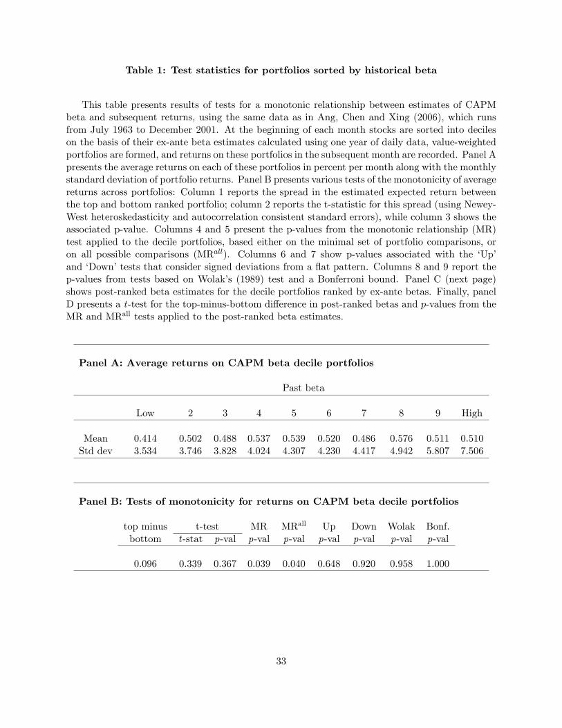
Table 1: Test statistics for portfolios sorted by historical beta
This table presents results of tests for a monotonic relationship between estimates of CAPMbeta and subsequent returns, using the same data as in Ang, Chen and Xing (2006), which runsfrom July 1963 to December 2001. At the beginning of each month stocks are sorted into decileson the basis of their ex-ante beta estimates calculated using one year of daily data, value-weightedportfolios are formed, and returns on these portfolios in the subsequent month are recorded. Panel Apresents the average returns on each of these portfolios in percent per month along with the monthlystandard deviation of portfolio returns. Panel B presents various tests of the monotonicity of averagereturns across portfolios: Column 1 reports the spread in the estimated expected return betweenthe top and bottom ranked portfolio; column 2 reports the t-statistic for this spread (using Newey-West heteroskedasticity and autocorrelation consistent standard errors), while column 3 shows theassociated p-value. Columns 4 and 5 present the p-values from the monotonic relationship (MR)test applied to the decile portfolios, based either on the minimal set of portfolio comparisons, oron all possible comparisons (MRall). Columns 6 and 7 show p-values associated with the �Up�and �Down�tests that consider signed deviations from a �at pattern. Columns 8 and 9 report thep-values from tests based on Wolak�s (1989) test and a Bonferroni bound. Panel C (next page)shows post-ranked beta estimates for the decile portfolios ranked by ex-ante betas. Finally, panelD presents a t-test for the top-minus-bottom di¤erence in post-ranked betas and p-values from theMR and MRall tests applied to the post-ranked beta estimates.
Panel A: Average returns on CAPM beta decile portfolios
Past beta
Low 2 3 4 5 6 7 8 9 High
Mean 0.414 0.502 0.488 0.537 0.539 0.520 0.486 0.576 0.511 0.510Std dev 3.534 3.746 3.828 4.024 4.307 4.230 4.417 4.942 5.807 7.506
Panel B: Tests of monotonicity for returns on CAPM beta decile portfolios
top minus t-test MR MRall Up Down Wolak Bonf.bottom t-stat p-val p-val p-val p-val p-val p-val p-val
0.096 0.339 0.367 0.039 0.040 0.648 0.920 0.958 1.000
33

Table 1: Test statistics for portfolios sorted by historical beta
See description on the previous page.
Panel C: Post-ranked betas on CAPM beta decile portfolios
Past beta
Low 2 3 4 5 6 7 8 9 High
0.600 0.659 0.702 0.774 0.856 0.850 0.904 1.013 1.194 1.539
Panel D: Tests of monotonicity for post-ranked beta estimates
top minus t-test MR MRall
bottom t-stat p-val p-val p-val
0.938 9.486 0.000 0.003 0.003
34
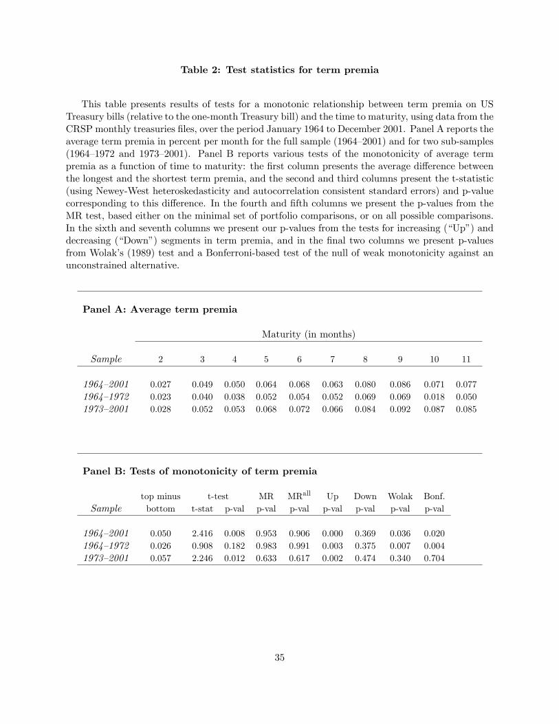
Table 2: Test statistics for term premia
This table presents results of tests for a monotonic relationship between term premia on USTreasury bills (relative to the one-month Treasury bill) and the time to maturity, using data from theCRSP monthly treasuries �les, over the period January 1964 to December 2001. Panel A reports theaverage term premia in percent per month for the full sample (1964�2001) and for two sub-samples(1964�1972 and 1973�2001). Panel B reports various tests of the monotonicity of average termpremia as a function of time to maturity: the �rst column presents the average di¤erence betweenthe longest and the shortest term premia, and the second and third columns present the t-statistic(using Newey-West heteroskedasticity and autocorrelation consistent standard errors) and p-valuecorresponding to this di¤erence. In the fourth and �fth columns we present the p-values from theMR test, based either on the minimal set of portfolio comparisons, or on all possible comparisons.In the sixth and seventh columns we present our p-values from the tests for increasing (�Up�) anddecreasing (�Down�) segments in term premia, and in the �nal two columns we present p-valuesfrom Wolak�s (1989) test and a Bonferroni-based test of the null of weak monotonicity against anunconstrained alternative.
Panel A: Average term premia
Maturity (in months)
Sample 2 3 4 5 6 7 8 9 10 11
1964�2001 0.027 0.049 0.050 0.064 0.068 0.063 0.080 0.086 0.071 0.0771964�1972 0.023 0.040 0.038 0.052 0.054 0.052 0.069 0.069 0.018 0.0501973�2001 0.028 0.052 0.053 0.068 0.072 0.066 0.084 0.092 0.087 0.085
Panel B: Tests of monotonicity of term premia
top minus t-test MR MRall Up Down Wolak Bonf.Sample bottom t-stat p-val p-val p-val p-val p-val p-val p-val
1964�2001 0.050 2.416 0.008 0.953 0.906 0.000 0.369 0.036 0.0201964�1972 0.026 0.908 0.182 0.983 0.991 0.003 0.375 0.007 0.0041973�2001 0.057 2.246 0.012 0.633 0.617 0.002 0.474 0.340 0.704
35

Table 3: Estimates of expected returns for decile portfolios
This table reports mean returns (in percent per month) for stocks sorted into value-weighteddecile portfolios. The sorting variables are market equity (ME), book-to-market value (BE-ME),cash �ow-price (CF-P), earnings-price (E-P), dividend-price (D-P), momentum (M�tum), shortterm reversal (ST Rev) and long term reversal (LT Rev). All data series are taken from KenFrench�s web site at Dartmouth. Panels A and B report results for the period 1963:07 �2006:12,while Panels C and D report results for the earliest available starting point for each series whichis 1926 or 1927 except for the portfolios sorted on long-term reversal which begin in 1931 andthe portfolios sorted on the earnings-price or cash�ow-price ratios which begin in 1951. Panels Band D report various tests for monotonicity in the average returns on these portfolios describedin Section 2. Row 1 reports the t-statistic for this spread (using Newey-West heteroskedasticityand autocorrelation consistent standard errors), and row 2 shows the associated p-value. Rows3 and 4 present the p-values from the monotonic relationship (MR) test between the portfoliosorting variables and expected returns across all decile portfolios, based either on the minimalset of portfolio comparisons, or on all possible comparisons (MRall). Rows 5 and 6 report the p-values from the bootstrap tests for �Up�and �Down�changes in expected returns across adjacentportfolios. The second-last and last rows report the p-values from Wolak�s (1989) test and a testbased on Bonferroni bounds.
ME BE-ME CF-P E-P D-P M�tum ST Rev LT Rev
Panel A: Average returns, 1963-2006
Low 1.273 0.824 0.850 0.829 1.002 0.177 1.147 1.3952 1.206 0.948 0.898 0.845 0.938 0.736 1.281 1.2443 1.241 0.989 0.975 0.975 1.029 0.862 1.255 1.2144 1.185 1.013 0.960 0.959 1.006 0.903 1.055 1.1045 1.209 1.014 1.069 0.943 0.912 0.801 1.020 1.1276 1.097 1.110 1.030 1.075 1.006 0.899 0.935 1.0747 1.151 1.188 1.090 1.234 1.045 0.941 0.890 1.0708 1.095 1.216 1.127 1.229 1.133 1.145 0.941 0.9779 1.026 1.269 1.329 1.284 1.122 1.238 0.748 0.897High 0.886 1.396 1.334 1.429 1.074 1.648 0.683 0.882High-Low -0.387 0.572 0.485 0.600 0.072 1.472 -0.464 -0.512
Panel B: Tests of monotonicity, 1963-2006
t-statistic -1.536 2.544 2.404 2.683 0.295 5.671 -2.364 -2.205t-test p-value 0.062 0.005 0.008 0.004 0.384 0.000 0.009 0.014MR p-value 0.274 0.000 0.024 0.008 0.336 0.291 0.258 0.002MRall p-value 0.237 0.000 0.012 0.021 0.256 0.242 0.170 0.002Up p-value 0.737 0.045 0.035 0.016 0.353 0.000 0.889 0.999Down p-value 0.051 1.000 0.994 0.985 0.651 0.954 0.015 0.114Wolak p-value 0.736 1.000 0.990 0.991 0.810 0.873 0.860 0.998Bonf. p-value 1.000 1.000 1.000 1.000 1.000 1.000 1.000 1.000
36
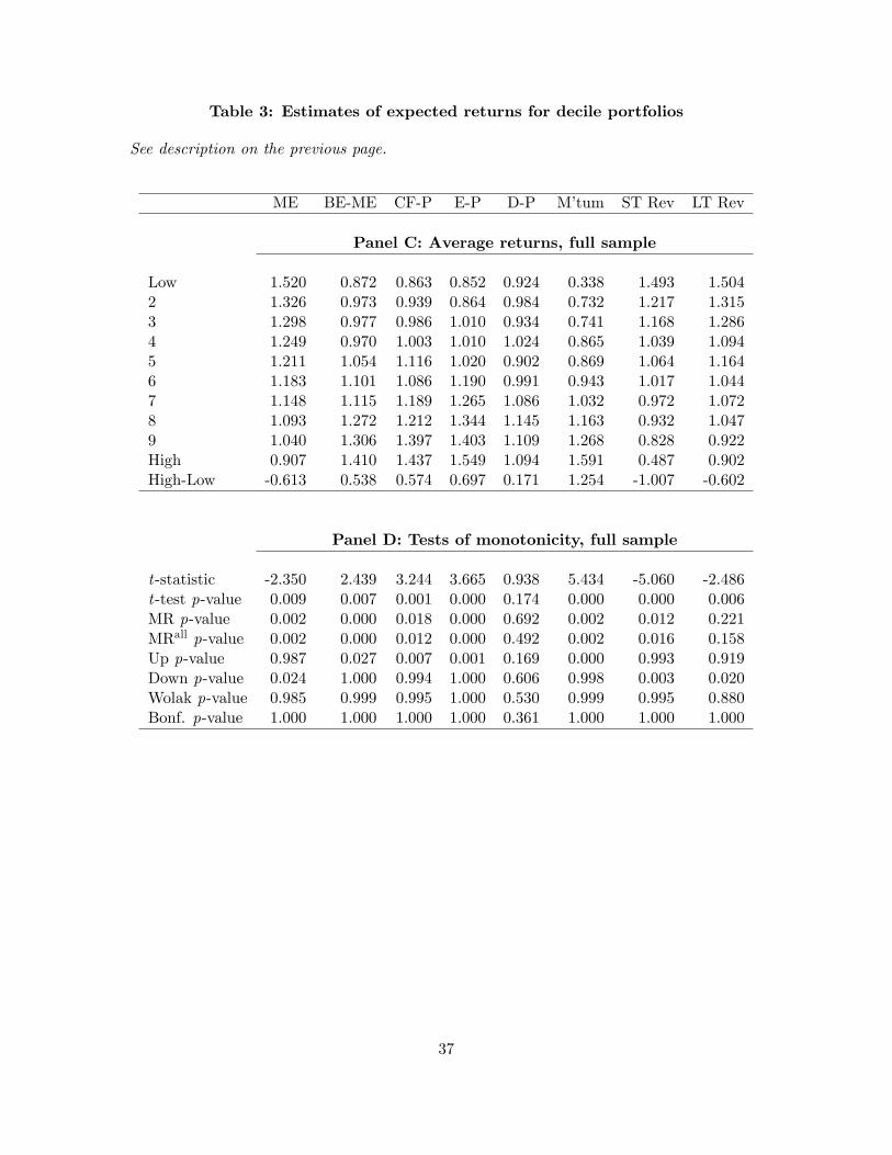
Table 3: Estimates of expected returns for decile portfolios
See description on the previous page.
ME BE-ME CF-P E-P D-P M�tum ST Rev LT Rev
Panel C: Average returns, full sample
Low 1.520 0.872 0.863 0.852 0.924 0.338 1.493 1.5042 1.326 0.973 0.939 0.864 0.984 0.732 1.217 1.3153 1.298 0.977 0.986 1.010 0.934 0.741 1.168 1.2864 1.249 0.970 1.003 1.010 1.024 0.865 1.039 1.0945 1.211 1.054 1.116 1.020 0.902 0.869 1.064 1.1646 1.183 1.101 1.086 1.190 0.991 0.943 1.017 1.0447 1.148 1.115 1.189 1.265 1.086 1.032 0.972 1.0728 1.093 1.272 1.212 1.344 1.145 1.163 0.932 1.0479 1.040 1.306 1.397 1.403 1.109 1.268 0.828 0.922High 0.907 1.410 1.437 1.549 1.094 1.591 0.487 0.902High-Low -0.613 0.538 0.574 0.697 0.171 1.254 -1.007 -0.602
Panel D: Tests of monotonicity, full sample
t-statistic -2.350 2.439 3.244 3.665 0.938 5.434 -5.060 -2.486t-test p-value 0.009 0.007 0.001 0.000 0.174 0.000 0.000 0.006MR p-value 0.002 0.000 0.018 0.000 0.692 0.002 0.012 0.221MRall p-value 0.002 0.000 0.012 0.000 0.492 0.002 0.016 0.158Up p-value 0.987 0.027 0.007 0.001 0.169 0.000 0.993 0.919Down p-value 0.024 1.000 0.994 1.000 0.606 0.998 0.003 0.020Wolak p-value 0.985 0.999 0.995 1.000 0.530 0.999 0.995 0.880Bonf. p-value 1.000 1.000 1.000 1.000 0.361 1.000 1.000 1.000
37
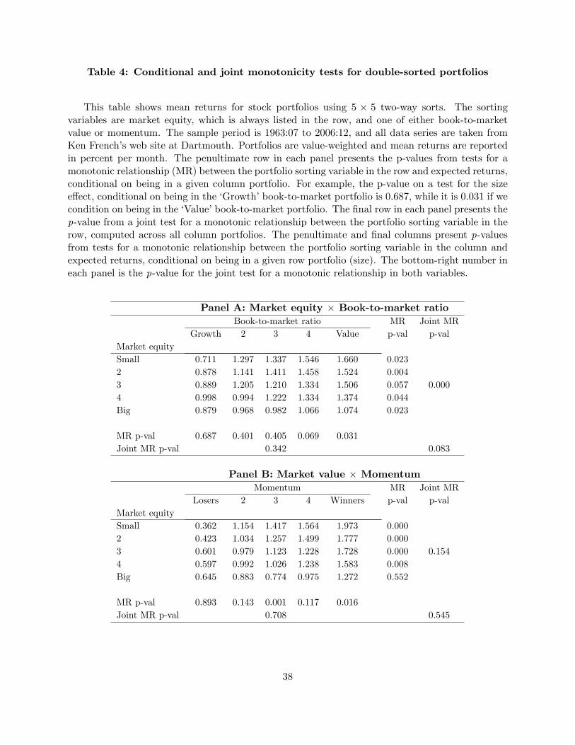
Table 4: Conditional and joint monotonicity tests for double-sorted portfolios
This table shows mean returns for stock portfolios using 5 � 5 two-way sorts. The sortingvariables are market equity, which is always listed in the row, and one of either book-to-marketvalue or momentum. The sample period is 1963:07 to 2006:12, and all data series are taken fromKen French�s web site at Dartmouth. Portfolios are value-weighted and mean returns are reportedin percent per month. The penultimate row in each panel presents the p-values from tests for amonotonic relationship (MR) between the portfolio sorting variable in the row and expected returns,conditional on being in a given column portfolio. For example, the p-value on a test for the sizee¤ect, conditional on being in the �Growth�book-to-market portfolio is 0.687, while it is 0.031 if wecondition on being in the �Value�book-to-market portfolio. The �nal row in each panel presents thep-value from a joint test for a monotonic relationship between the portfolio sorting variable in therow, computed across all column portfolios. The penultimate and �nal columns present p-valuesfrom tests for a monotonic relationship between the portfolio sorting variable in the column andexpected returns, conditional on being in a given row portfolio (size). The bottom-right number ineach panel is the p-value for the joint test for a monotonic relationship in both variables.
Panel A: Market equity � Book-to-market ratioBook-to-market ratio MR Joint MR
Growth 2 3 4 Value p-val p-valMarket equitySmall 0.711 1.297 1.337 1.546 1.660 0.0232 0.878 1.141 1.411 1.458 1.524 0.0043 0.889 1.205 1.210 1.334 1.506 0.057 0.0004 0.998 0.994 1.222 1.334 1.374 0.044Big 0.879 0.968 0.982 1.066 1.074 0.023
MR p-val 0.687 0.401 0.405 0.069 0.031Joint MR p-val 0.342 0.083
Panel B: Market value � MomentumMomentum MR Joint MR
Losers 2 3 4 Winners p-val p-valMarket equitySmall 0.362 1.154 1.417 1.564 1.973 0.0002 0.423 1.034 1.257 1.499 1.777 0.0003 0.601 0.979 1.123 1.228 1.728 0.000 0.1544 0.597 0.992 1.026 1.238 1.583 0.008Big 0.645 0.883 0.774 0.975 1.272 0.552
MR p-val 0.893 0.143 0.001 0.117 0.016Joint MR p-val 0.708 0.545
38

Table 5: Monte Carlo simulation results
This table reports rejection frequencies for simulated data repeatedly drawn from the value-weighted decile portfolios sorted on market equity, using 2500 Monte Carlo simulations and 1000bootstraps for each simulation. The columns report the proportion of rejections from tests ofmonotonicity, with nominal size of 0.05. Columns 1 and 2 report the proportion of rejections froma t-test applied to the spread in expected returns between the top and bottom portfolios, and fromthe monotonic relationship (MR) test, respectively. These results are obtained under the normalityassumption discussed in Section 4. Columns 3 to 9 show the corresponding proportions of rejectionsusing bootstrapped portfolio data based on the value-weighted decile portfolios sorted on marketequity. Column 3 is a standard t-test applied to the spread in expected returns between the top andbottom portfolios. The fourth and �fth columns report the proportion of rejections using the MRtest based on the minimal set of possible inequalities (MR) or all possible inequalities implied bymonotonicity (MRall). The sixth and seventh columns report the proportion of rejections of the nullof no relationship against the alternative that the sum of positive (Up) or absolute values of negative(Down) di¤erences in expected returns is non-zero. The last two columns (Wolak and Bonf) reportthe proportion of rejections of the null of a weakly monotonic relationship using Wolak�s (1989)test, with critical values based on 1000 simulations per replication, and a Bonferroni bound test.
�Step� refers to the step size in percent per month used in forming the spreads in expectedreturns on the decile portfolios. Experiments I-III impose a monotonic relation between portfoliorank and expected returns, while experiments IV-VIII impose a non-monotonic pattern. Figure 3displays the shapes of the assumed patterns. The experiments are identical when the step size iszero and so only the results for Experiment I are presented in that case.
Table 5 is on the following page.
39
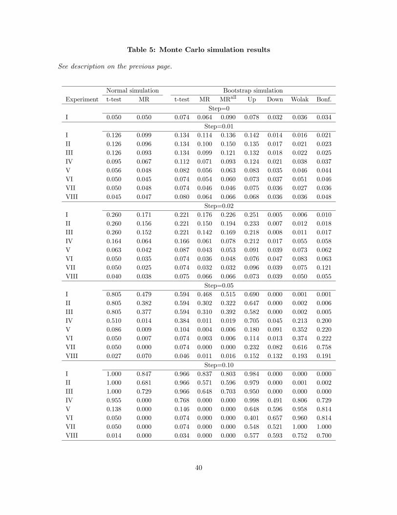
Table 5: Monte Carlo simulation results
See description on the previous page.
Normal simulation Bootstrap simulationExperiment t-test MR t-test MR MRall Up Down Wolak Bonf.
Step=0I 0.050 0.050 0.074 0.064 0.090 0.078 0.032 0.036 0.034
Step=0.01I 0.126 0.099 0.134 0.114 0.136 0.142 0.014 0.016 0.021II 0.126 0.096 0.134 0.100 0.150 0.135 0.017 0.021 0.023III 0.126 0.093 0.134 0.099 0.121 0.132 0.018 0.022 0.025IV 0.095 0.067 0.112 0.071 0.093 0.124 0.021 0.038 0.037V 0.056 0.048 0.082 0.056 0.063 0.083 0.035 0.046 0.044VI 0.050 0.045 0.074 0.054 0.060 0.073 0.037 0.051 0.046VII 0.050 0.048 0.074 0.046 0.046 0.075 0.036 0.027 0.036VIII 0.045 0.047 0.080 0.064 0.066 0.068 0.036 0.036 0.048
Step=0.02I 0.260 0.171 0.221 0.176 0.226 0.251 0.005 0.006 0.010II 0.260 0.156 0.221 0.150 0.194 0.233 0.007 0.012 0.018III 0.260 0.152 0.221 0.142 0.169 0.218 0.008 0.011 0.017IV 0.164 0.064 0.166 0.061 0.078 0.212 0.017 0.055 0.058V 0.063 0.042 0.087 0.043 0.053 0.091 0.039 0.073 0.062VI 0.050 0.035 0.074 0.036 0.048 0.076 0.047 0.083 0.063VII 0.050 0.025 0.074 0.032 0.032 0.096 0.039 0.075 0.121VIII 0.040 0.038 0.075 0.066 0.066 0.073 0.039 0.050 0.055
Step=0.05I 0.805 0.479 0.594 0.468 0.515 0.690 0.000 0.001 0.001II 0.805 0.382 0.594 0.302 0.322 0.647 0.000 0.002 0.006III 0.805 0.377 0.594 0.310 0.392 0.582 0.000 0.002 0.005IV 0.510 0.014 0.384 0.011 0.019 0.705 0.045 0.213 0.200V 0.086 0.009 0.104 0.004 0.006 0.180 0.091 0.352 0.220VI 0.050 0.007 0.074 0.003 0.006 0.114 0.013 0.374 0.222VII 0.050 0.000 0.074 0.000 0.000 0.232 0.082 0.616 0.758VIII 0.027 0.070 0.046 0.011 0.016 0.152 0.132 0.193 0.191
Step=0.10I 1.000 0.847 0.966 0.837 0.803 0.984 0.000 0.000 0.000II 1.000 0.681 0.966 0.571 0.596 0.979 0.000 0.001 0.002III 1.000 0.729 0.966 0.648 0.703 0.950 0.000 0.000 0.000IV 0.955 0.000 0.768 0.000 0.000 0.998 0.491 0.806 0.729V 0.138 0.000 0.146 0.000 0.000 0.648 0.596 0.958 0.814VI 0.050 0.000 0.074 0.000 0.000 0.401 0.657 0.960 0.814VII 0.050 0.000 0.074 0.000 0.000 0.548 0.521 1.000 1.000VIII 0.014 0.000 0.034 0.000 0.000 0.577 0.593 0.752 0.700
40
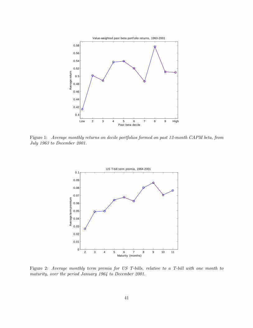
Low 2 3 4 5 6 7 8 9 High
0.4
0.42
0.44
0.46
0.48
0.5
0.52
0.54
0.56
0.58
Ave
rage
retu
rn
Past beta decile
Valueweighted past beta portf olio returns, 19632001
Figure 1: Average monthly returns on decile portfolios formed on past 12-month CAPM beta, fromJuly 1963 to December 2001.
2 3 4 5 6 7 8 9 10 110
0.01
0.02
0.03
0.04
0.05
0.06
0.07
0.08
0.09
0.1US Tbill term premia, 19642001
Maturity (months)
Ave
rage
term
pre
miu
m
Figure 2: Average monthly term premia for US T-bills, relative to a T-bill with one month tomaturity, over the period January 1964 to December 2001.
41
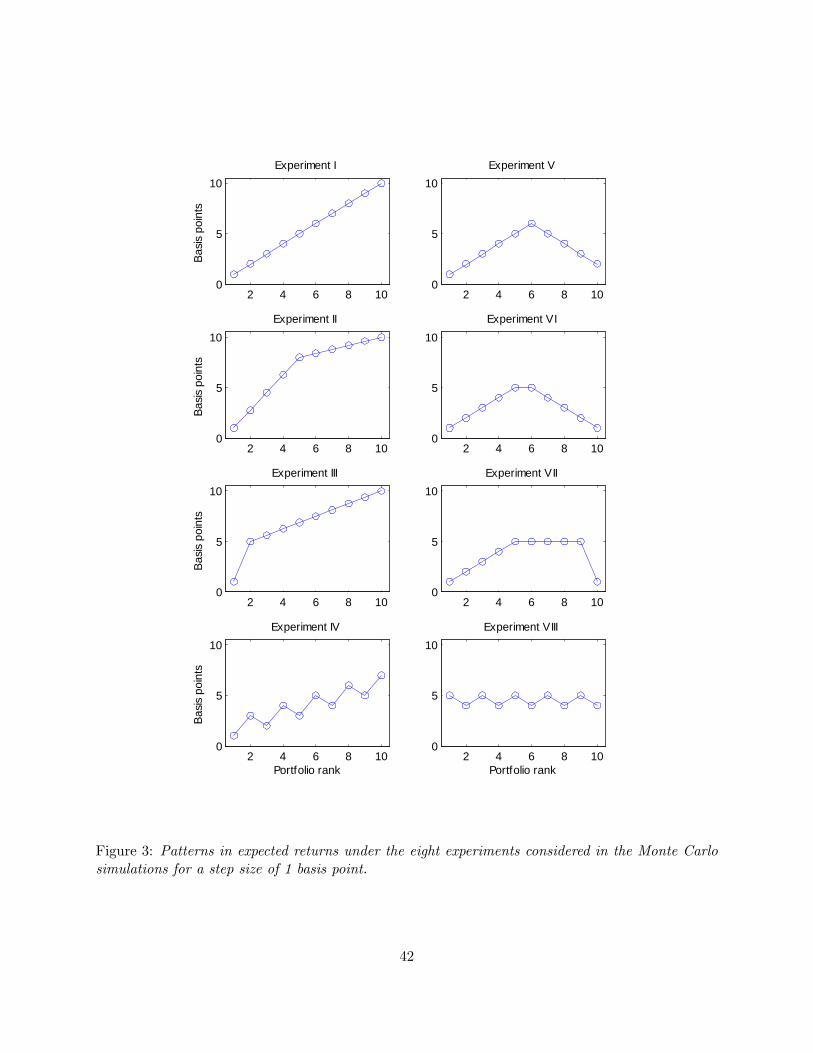
2 4 6 8 100
5
10
Experiment I
Bas
is p
oint
s
2 4 6 8 100
5
10
Experiment V
2 4 6 8 100
5
10
Experiment II
Bas
is p
oint
s
2 4 6 8 100
5
10
Experiment VI
2 4 6 8 100
5
10
Experiment III
Bas
is p
oint
s
2 4 6 8 100
5
10
Experiment VII
2 4 6 8 100
5
10
Experiment IV
Portfolio rank
Bas
is p
oint
s
2 4 6 8 100
5
10
Experiment VIII
Portfolio rank
Figure 3: Patterns in expected returns under the eight experiments considered in the Monte Carlosimulations for a step size of 1 basis point.
42


![A cross-cultural analysis of the returns of Local ...icta.uab.cat/Etnoecologia/Docs/[423]-lektests.pdf · KNOWLEDGE AND SKILLS TESTS The adaptive nature of culture: A cross-cultural](https://img.pdfslide.tips/doc/110x75/5acf34eb7f8b9ae2138c3ddf/a-cross-cultural-analysis-of-the-returns-of-local-ictauabcatetnoecologiadocs423-.jpg)