arX

iv:a

stro

-ph/

0610

118v

1 4

Oct

200

6PASJ: Publ. Astron. Soc. Japan , 1–??,c© 2018. Astronomical Society of Japan.

Monte-Carlo Simulator and Ancillary Response Generator of Suzaku

XRT/XIS System for Spatially Extended Source Analysis

Yoshitaka Ishisaki,1 Yoshitomo Maeda,2 Ryuichi Fujimoto,2 Masanobu Ozaki,2

Ken Ebisawa,2 Tadayuki Takahashi,2 Yoshihiro Ueda,3 Yasushi Ogasaka,4

Andrew Ptak,5 Koji Mukai,6 Kenji Hamaguchi,6 Masaharu Hirayama,6 Taro Kotani,7

Hidetoshi Kubo,8 Ryo Shibata,4 Masatoshi Ebara,2 Akihiro Furuzawa,4 Ryo Iizuka,9 Hirohiko Inoue,2

Hideyuki Mori,8 Shunsaku Okada,2 Yushi Yokoyama,2 Hironori Matsumoto,8 Hiroshi Nakajima,8

Hiroya Yamaguchi,8 Naohisa Anabuki,10 Noriaki Tawa,10 Masaaki Nagai,10 Satoru Katsuda,10

Kiyoshi Hayashida,10 Aya Bamba,11 Eric D. Miller,12 Kousuke Sato,1 Noriko Y. Yamasaki 21 Department of Physics, Tokyo Metropolitan University, 1-1 Minami-Osawa, Hachioji, Tokyo 192-0397

ishisaki@phys.metro-u.ac.jp2 Institute of Space and Astronautical Science (ISAS), JAXA, 3-1-1 Yoshinodai, Sagamihara, Kanagawa 229-8510

3 Department of Astronomy, Kyoto University, Sakyo-ku, Kyoto 606-85024 Department of Particle and Astrophysics, Nagoya University, Furo-cho, Chikusa-ku, Nagoya 464-8602

5 Department of Physics and Astronomy, Johns Hopkins University,

3400 North Charles Street, Baltimore, MD 21218-2686, USA6 NASA/Goddard Space Flight Center, Greenbelt, MD 20771, USA

7 Department of Physics, Tokyo Institute of Technology, 2-12-1 O-okayama, Meguro-ku, Tokyo 152-85518 Department of Physics, Kyoto University, Sakyo-ku, Kyoto 606-85029 Nishi-Harima Astronomical Observatory, Sayo-cho, Hyogo 679-5313

10 Department of Earth and Space Science, Osaka University, 1-1 Machikane-yama, Toyonaka, Osaka 560-004311 The Institute of Physical and Chemical Research (RIKEN), 2-1 Hirosawa, Wako, Saitama 351-0198

12 Kavli Institute for Astrophysics and Space Research, Massachusetts Institute of Technology, Cambridge, MA 02139, USA

(Received 2006 September 6; accepted 2006 September 29)

Abstract

We have developed a framework for the Monte-Carlo simulation of the X-Ray Telescopes (XRT) andthe X-ray Imaging Spectrometers (XIS) onboard Suzaku, mainly for the scientific analysis of spatially andspectroscopically complex celestial sources. A photon-by-photon instrumental simulator is built on theANL platform, which has been successfully used in ASCA data analysis. The simulator has a modularstructure, in which the XRT simulation is based on a ray-tracing library, while the XIS simulation uti-lizes a spectral “Redistribution Matrix File” (RMF), generated separately by other tools. Instrumentalcharacteristics and calibration results, e.g., XRT geometry, reflectivity, mutual alignments, thermal shieldtransmission, build-up of the contamination on the XIS optical blocking filters (OBF), are incorporatedas completely as possible. Most of this information is available in the form of the FITS (Flexible ImageTransport System) files in the standard calibration database (CALDB). This simulator can also be utilizedto generate an “Ancillary Response File” (ARF), which describes the XRT response and the amount ofOBF contamination. The ARF is dependent on the spatial distribution of the celestial target and thephoton accumulation region on the detector, as well as observing conditions such as the observation dateand satellite attitude. We describe principles of the simulator and the ARF generator, and demonstratetheir performance in comparison with in-flight data.

Key words: Instrumentation: detectors — Telescopes — X-rays: general — Methods: data analysis

1. Introduction

A Monte-Carlo simulator is useful in characterizing adetector, and can relatively easily take into account manyof the parameters which affect observations. Since the ul-timate goal of X-ray data analysis is to estimate the truetime, energy and position of the incoming X-ray photons,it is quite important to predict precisely how the photonsinteract with the telescope and detector. A good simula-tor is therefore strongly required not only for instrumental

calibration and proposal planning, but also for scientificanalysis. Chandra and XMM-Newton also have good sim-ulators, named MARX 1 and SciSim 2, respectively.The X-ray observatory Suzaku (formerly known as

Astro-E2) is the fifth Japanese X-ray astronomy satel-lite (Mitsuda et al. 2006). It has been developed under aJapan–US international collaboration, and was launched

1 http://space.mit.edu/ASC/MARX/2 http://xmm.vilspa.esa.es/scisim/

2 Y. Ishisaki et al. [Vol. ,

on 2005 July 10. Five X-Ray telescopes are present, sen-sitive to soft X-rays below ∼ 10 keV (XRTs; Serlemitsoset al. 2006). At the foci of four of the XRTs (XRT-I)are charge-coupled devices (CCD), known as the X-rayImaging Spectrometers (XIS; Koyama et al. 2006); one(XRT-S) is combined with an X-ray calorimater known asthe X-Ray Spectrometer (XRS; Kelley et al. 2006; XRSquit operation ∼ 1 month after the launch).The Suzaku XRT is characterized by large collective

area and relatively short focal lengths, compared withthose ofChandra andXMM-Newton. In combination withthese features, the low-earth orbit of Suzaku, where theparticle background is low and stable, makes the non-X-ray background (NXB) of Suzaku much lower comparedwith Chandra and XMM-Newton. In addition, the XISachieves good spectral resolution, especially at the low en-ergy range below ∼ 1 keV with the backside-illuminated(BI) CCD for XIS1. The front-illuminated (FI) CCDsfor XIS0, XIS2, and XIS3 exhibit about half of the NXBrate than XIS1 (and less at energies >∼ 8 keV), so they arecomplementary. Therefore, Suzaku has a unique advan-tage for spectroscopic observations of spatially extendedsources (Mitsuda et al. 2006).To achieve large collective area within the tight weight

budget (1706 kg), the Suzaku XRT adopts the conicalapproximation of Wolter type I optics with 175 layers ofthe thin-foil-nested reflectors per quadrant (Serlemitsos etal. 2006). In return for the high throughput, it providesa moderate imaging capability of 2′ half power diameterwith a complex point spread function (PSF), as well asthe energy-dependent vignetting effects common to X-raytelescopes. In addition, there exists spatially-dependentcontamination on the optical blocking filters (OBF) of theXIS (Koyama et al. 2006). These XRT and XIS character-istics often make extended source analysis complicated, soit is crucial to prepare a tool in order to precisely evaluatethe effect of complex telescope and detector responses.We developed a Monte-Carlo simulator of the Suzaku

XRT/XIS system, which is incorporated into two practi-cal tools, the XIS simulator “xissim” and the “AncillaryResponse File” (ARF) generator “xissimarfgen”. The sim-ulator is constructed on the “ANL” platform (§ 2.1), whichis used for almost all of the processing and analysis soft-ware of Suzaku.While these tasks provide vast flexibility to the Suzaku

XIS users, it is rather difficult to utilize them efficientlyand appropriately. For example, there are more than 90parameters for both xissim and xissimarfgen. There areseveral issues and limitations that one should be awareof in running these tasks. This paper is aimed to clarifythese things by explaining principles of the software andby demonstrating performance with practical examples.We have also tried to separate the ‘calibration issues’,which can be changed (usually improved) by calibrationupdates, from those originated in the design of the soft-ware itself. The quality of the calibration is out of scopefor this paper, although some aspects are discussed brieflyin § 6.This paper is organized as follows. In § 2, we briefly

show the strategy of the Suzaku software development, fo-cusing on the ANL platform and simulators. In § 3 and § 4,we describe principles of xissim and xissimarfgen, respec-tively. In § 5, several notes on these tasks are described.In § 6, we demonstrate these tasks with three distinct ex-amples, the Crab Nebula, the North Ecliptic Pole (NEP)field, and Abell 1060. Finally, a summary is given in § 7.We also added three appendices which describe the coor-dinates definition, structures, parameters, and the outputfile formats, in detail.

2. Software Development for Suzaku

2.1. The ANL Platform

When ASTRO-E software development started in 1995,the goal was a common software framework/platformwhich is used by realtime quick-look, data processing, andscientific analysis, both during pre-launch phase and af-ter the launch. To that end, it was necessary to providea common programming environment where instrumentteam members can easily develop, maintain and updatessoftwares that they need. This framework/platform alsomust allow end-users to share these softwares. The frame-work must be easy to learn for instrument team members,who, spending most of the time in calibrating the instru-ments, do not necessarily have extensive programming ex-perience. Also, from the end users’ point of view, it is de-sirable that those software tools developed based on thisframework are maximally flexible and have an Ftools-like simple interface which is familiar to most X-ray as-tronomers.A software platform called “ASCA ANL”, which had

been developed for the ASCA satellite (Tanaka etal. 1994), fulfills these requirements. The ASCA ANLplatform mandates modular design of the analysis soft-ware to be built upon it, and makes the software prod-ucts easily configurable and reusable in components, sothat software developers and end-users can share the samecomponents for different purposes. This feature not onlyreduces code duplication, but also helps to quickly matureand refine the software.Indeed, ASCA ANL fostered many practical tools in-

cluding the instrument simulator SimASCA and theresponse generator SimARF. The advantages of theASCA ANL platform are demonstrated by original sci-entific research which would have been difficult withoutSimASCA and SimARF; e.g., spatial-spectral analysis ofclusters of galaxies (Ikebe et al. 1996; Honda et al. 1996),systematic analysis of large volumes of X-ray surveys andthe cosmic X-ray background (Ueda et al. 1998; Uedaet al. 1999; Kushino et al. 2002). The SimASCA andSimARF were very helpful to realize a specialized anal-ysis method in the analysis of spatially extended sources(which is not supported by standard analysis software),and to accurately compute complicated instrument re-sponses.On the other hand, however, ASCA ANL and other rel-

evant software were based on the functions and librariesused for realtime quick-look software which had been de-

No. ] Suzaku XRT/XIS Simulator & ARF Generator 3

veloped by the instrument teams, independently from theofficial ASCA analysis software (Ftools). This resultedin two independent streams to calculate basic physical val-ues from the raw data, such as the pulse height correctedfor the detector gain changes (known as “pulse invariant”,or PI, corresponding to the detected photon energy), andthe sky and detector coordinates of events, which causedconfusion in the scientific analysis of the ASCA data.Based on the ASCA experience, we adopted the “ANL”,

i.e. a generalized version of the ASCA ANL, as the soft-ware development platform for ASTRO-E and Suzaku.A brief history and concept of the ANL are describedin Ozaki et al. (2006). At the same time, we devel-oped a mechanism to convert ANL software directly toFtools, to ensure that the ANL tools used for calibrationby instrument teams are equivalent to Ftools used forpipeline processing and scientific data analysis. CommonFITS-read and -write ANL modules and functions werealso developed to handle photon event files and the cal-ibration files in FITS format.3 Now, almost all of theFtools for Suzaku including xissim and xissimarfgen, re-leased from the Guest Observer Facility at NASA/GSFC,are developed in the ANL framework.

2.2. History of Suzaku Simulators

The development of the Suzaku simulator had startedbefore the failure launch of the ASTRO-E on 10 Feb2000, especially for the bilinear 16× 2 pixel XRS detec-tor (Kelley et al. 1999). The detector size was compara-ble with the angular resolution of the XRT (Kunieda etal. 2001; Shibata et al. 2001), and so the XRS PSF wasundersampled. The energy resolution of the XRS was alsovery dependent on the count rate of each calorimeter pixel.Therefore, the XRT/XRS system simulator, xrssim, wasrequired to estimate the flux coming to each XRS pixel,which was critical for proposal planning. This was also thecase for the Suzaku XRS. The xissim task subsequentlydeveloped by replacing the XRS component of the simu-lator with the XIS component.The XRT ray-tracing part of the simulator has been sig-

nificantly updated from the ASCA era. The code had beenrewritten, by R. L. Fink (NASA/GSFC), from Fortraninto C++, and the structure had been re-designed toutilize the mirror geometry and reflectivity files as sep-arate calibration FITS files. This ray-tracing code is nowsupplied as the “xrrt” library by the XRT team. It hasbeen utilized for the performance improvement of the XRT(Misaki et al. 2005) and the design of the pre-collimatorto suppress the stray-light (Mori et al. 2005).At present, xissim and xissimarfgen are publicly re-

leased in the Suzaku Ftools and all the source codeis available including the ANL itself and the xrrt li-brary. The latest version of the xissim package is 2006-08-26, which will be included in the next official release ofthe Suzaku Ftools for version 2.0 processing of Suzakuarchival data scheduled in late 2006. All the calibration

3 The calibration FITS files are released to the public from theNASA/GSFC guest observer facility, as part of the official cali-bration database (CALDB; George et al. 1991).

information currently available is taken into account viathe CALDB calibration database. The mkphlist, xissim,xissimarfgen, and xiscontamicalc tasks described in thispaper are based on this version of the xissim package.The latest information on the xissim package is availableat http://www-x.phys.metro-u.ac.jp/˜ishisaki/xissim/.We also note that there is another Monte Carlo simu-

lator for Suzaku, based on the Geant4 toolkit (Geant4Collaboration et al. 2003) with ANL++ (Ozaki etal. 2006). This can simulate interactions of cosmic rays(both X/γ-rays and particles) with the satellite materials,such as satellite structures, shielding around detectors,and the detectors themselves. The main purpose of thissimulator is to study response of the Hard X-ray Detector(HXD; Takahashi et al. 2006; Kokubun et al. 2006), andthe NXB models for both HXD and XIS. See Terada etal. (2005) and Ozaki et al. (2006) for details.

3. Simulator: xissim

The xissim task simulates the interaction of the incidentX-ray photons with the XRT/XIS system, using the XRTray-tracing library and a spectral “Redistribution MatrixFile” (RMF; see § 4.1) for the XIS, and generates a sim-ulated event file. The format of the generated event fileis a stripped-down version of that created by the pipelineprocessing of a real observation, so that users can analyzethe simulated data in the same manner as the real data.To perform the simulation, users need to take three steps.First, the spatial distribution and the energy spectrumof the celestial source to be simulated must be specified.Second, a list of incident photons from the source needs tobe prepared as FITS file(s). An auxiliary tool, mkphlist,may be used for this purpose. Third, the photon FITSfile is passed to xissim, which then performs a photon-by-photon simulation, and creates a file of events detectedby the XIS. In the following subsections, we describe howxissim performs the simulation.

3.1. Photon Generation

An auxiliary task mkphlist generates a list of fakedphotons of an X-ray source from the model spectralenergy and spatial distribution, photon flux (in pho-tons cm−2 s−1) in an arbitrary energy band, and the ge-ometrical area of the XRT (in cm2), provided by users.A model spectral distribution file (which is specified bythe qdp spec file parameter) must be in units of photonflux (photons cm−2 s−1 keV−1) that can be easily pro-duced with standard software packages such as Xspec(Arnaud 1996). mkphlist requires celestial coordinates ofthe point source or a surface brightness map (FITS image)on the sky for the spatial distribution of the source. Eitherthe number of photons or exposure time is needed to de-termine how many photons are to be generated. Users canalso specify equal or random interval steps for the photonarrival time. The structure of mkphlist is explained inAppendix 2.1, and a list of major parameters and the for-mat of the photon file are summarized in table 5 and 8,respectively. Note that, by preparing an appropriate pho-

4 Y. Ishisaki et al. [Vol. ,

ton file, users can in principle simulate any source withany energy spectrum and/or any spatial distribution.

3.2. Photon-by-Photon Simulation

By taking into account the XRT and XIS response, xis-sim performs photon-by-photon simulation for given inputphoton file(s). It has the capability to read up to eightphoton files simultaneously. Figure 1 shows the schematicstructure of the simulation implemented in xissim. Sinceunderstanding the coordinate systems is essential, we in-clude the definitions in Appendix 1.First of all, the ra and dec values in the photon file

need to be converted to (θ, φ), i.e. offset angle (′) andazimuth angle (◦), with respect to the XRT optical axis.This requires the satellite Euler angles (ea1, ea2, ea3) (

◦),the observation date for an aberration correction (or par-allax correction, see Appendix 1), and the alignment pa-rameters in the telescope definition (teldef ) file. Userscan supply an attitude file (set of Euler angles as a func-tion of time) and a good time interval (GTI) file to takeinto account the wobbling of the spacecraft (See also § 5.2for the attitude wobbling). The photon time columnin the photon file usually starts from 0.0 s unless other-wise specified, and it is treated as the time offset relativeto the GTI. Alternatively one may specify a fixed setof Euler angles and/or a fixed date. The aberration cor-rection can be disabled by setting the hidden parameteraberration=no (hidden parameters are not required wheninvoking an Ftools task).In the second stage, the geometrical area for a given

photon is reduced by a factor of cosθ due to the slantedincidence to the XRT. This factor is usually very closeto unity, and had been neglected in the older version ofxissim. This behavior can be controlled with the param-eter aperture cosine, and is set to ‘yes’ by default in thepresent version. The photon flux is further reduced dueto transmission through the thermal shield on the top ofthe XRT. Xissim then assigns a random location for eachphoton at the top surface of the XRT, where the pre-collimator is placed. The task traces the path of eachphoton inside the XRT (pre-collimator, primary and sec-ondary mirrors), using the XRT ray-tracing library, xrrt(Misaki et al. 2005;Mori et al. 2005), using the XRT geom-etry and reflectivity as described in the ray-tracing codeand the calibration files. After the ray-tracing, some pho-tons may be absorbed and disappear, while others reachthe focal plane.A fraction of the photons that have reached the focal

plane are absorbed by the contamination on the OBF.The thickness of the contamination is time- and detector-position-dependent (Koyama et al. 2006), and their de-pendence is given by a calibration file supplied by theXIS team. Xissim computes the transmissivity at a giventime and position using this calibration file. The positionof the photon on the detector is again calculated by thealignment parameters in the teldef file.Finally, the simulated photons reach the detector (in-

cluding both OBF and CCD), where the detection prob-ability is determined using the RMF of the XIS. The

Fig. 1. Schematic structure of the simulation.

XIS RMF contains the transmission of the OBF and thequantum efficiency of the CCD, as well as the spectral re-distribution matrix from energy to PI. The line responsefunction of the XIS CCDs is primarily a Gaussian distri-bution but it also includes other features such as escaperatios and tails that deviate from a Gaussian. Photonsthat have passed the test for detection are recorded asX-ray events,4 and their PI values are determined fromthe incident photon energy by random choices accord-ing to the energy redistribution probability in the RMF.The Suzaku XIS detectors do not exhibit significant posi-tional dependence in the energy resolution after the CTI(charge transfer inefficiency) correction while the energyresolution is known to degrade with time. Users shouldsupply an appropriate RMF corresponding to the obser-vation date, which can be generated by a separate task,xisrmfgen.Note that the current version of xissim does not consider

the NXB, bad CCD columns, event pile-up, event grade,nor CCD exposure frames. Although the output event

4 We shall call ‘photon’ during the simulation, which becomes‘event’ after the detection.

No. ] Suzaku XRT/XIS Simulator & ARF Generator 5

files contains the same major columns as the event files ofthe real data, the status and grade columns are filledwith 0, while the pha column has the same value as thepi column.The ANL module structure and parameters of xissim

is explained in Appendix 2.2 in detail. If one has theANL programing environment available, he/she may addhis/her own modules to the simulator. It is also easy toreplace a module, e.g. if a module is available that moreprecisely simulates the CCD detection process, then thismodule can be substituted for the SimASTE XISRMFsimmodule which utilizes a ready-made RMF. This is one ofthe great benefits of the ANL.

3.3. Calibration Files

Table 1 summarizes the list of calibration files used byxissim. The file specified by the leapfile parameter is theleap second file, and is required to compute the missiontime (or Suzaku time), defined as accumulative secondssince 2000 January 1, 00:00:00 (UTC). In fact, the de-fault value of the leapfile parameter is set to a specialkeyword of “caldb” and is a hidden parameter. By in-stalling CALDB and properly setting the environmentalvariables, the xissim task automatically searches the mostrecent calibration file for this category, i.e. ‘Content Name’= leapsecs. This is also applicable to other parametersin table 1.The shieldfile, mirrorfile, reflectfile, and backproffile pa-

rameters are used for the XRT simulation. There are fourFITS extensions in the mirrorfile to describe the geome-try of each XRT, and three extensions are present in thereflectfile corresponding to materials of the reflection sur-face. As described in Appendix 1, teldef is used to describethe mutual alignments between XRT and XIS, as well asamong the XIS sensors and the spacecraft. The contam-

ifile describes the energy, time, and position dependenceof the contamination on the XIS OBF.

4. Ancillary Response Generator: xissimarfgen

The xissimarfgen task generates a Suzaku XIS ARFbased on user-defined conditions, such as an arbitraryshape of the X-ray emitting region and event extractionregions. Xissimarfgen does so by simulating photon de-tections at each energy. It then calculates the detectionefficiency in a user-defined event accumulation region.5

Since it utilizes a Monte-Carlo simulation, users need tosimulate enough photons to avoid counting statistics er-rors. It can refer to the attitude file to reflect the changeof effective area due to the attitude wobbling. The finalARF is in the standard FITS format, so that users canuse Xspec or other standard fitting packages for spectralanalysis.

4.1. Principle of ARF Calculation and Limitations

The ARF is utilized for spectral fitting combined withan RMF. See George et al. (1992) for detailed format

5 We shall use ‘accumulate’ for the simulated events, and ‘extract’for the real observed events.

of these files. The RMF is represented by an (m× n)matrix R(Ei,PI j), where E (keV) denotes the energyand PI (channel; hereafter chan) denotes the pulse in-variant, with 1≤ i≤m and 1≤ j ≤n. Regarding the XIS,m = 7900, n = 4096, E1 = 0.201 keV, Em = 15.999 keV,PI 1 =0 chan, and PI n =4095 chan for the nominal RMF.The ARF is represented by anm-dimensional vector whichwe denote as S A(Ei) (cm

2), where S = 1152.41 cm2 rep-resents the geometrical area of the XRT. The goal of thespectral fitting is to find a model spectrum, M(Ei) (pho-tons cm−2 s−1 keV−1), which fits the observed spectrum,D(PI j) (count cm

−2 s−1). The response and model spec-trum are convolved, i.e.,

M(PI j) = Sm∑

i=1

∆Ei A(Ei)R(Ei,PI j)M(Ei), (1)

where ∆E (keV) is the energy bin width, and M(PI j)and D(PI j) are compared. As one can see easily fromthis formula, [A(Ei)R(Ei,PI j) ] represents an expectedspectrum for the monochromatic X-ray of E=Ei keV, and

A(Ei)

n∑

j=1

R(Ei,PI j) represents the detection efficiency at

E = Ei keV.Thus, calculating the ARF is reduced to the computa-

tion of the detection efficiency at each energy step, Ei,of the RMF, a job well-suited for a Monte-Carlo simu-lation. For a given input Nin counts of monochromaticX-ray photons at E =Ei keV, the simulator predicts Ndet

detected events and then the detection efficiency is simplyA(Ei) =Ndet/Nin. However, one must be very careful be-cause the detection efficiency, namely Ndet, is influencedby many factors: first of all, the accumulation region ofthe event on the detector, and the spatial distribution ofthe celestial sources assumed on the sky. It is also affectedby the observational conditions, such as the satellite Eulerangles, the date of the observation due to the thickness ofthe XIS contamination and the parallax correction, etc.The quality of the calibration and/or the Poisson statisticscan also impact Ndet. It is therefore important that onemust reproduce the user-selection and the observationalconditions of the real data as much as possible in the sim-ulation. One must also take care to perform a simulationsuch that the photon statistics are sufficiently better thanthe statistics of the real observation.In fact, the spatial distribution on the sky is sometimes

complex and/or extended on a scale larger than the tele-scope FOV. Thus the accuracy of the spatial model canbecome a major cause of systematic error in the estima-tion of the detection efficiency, which leads to uncertaintyin the source flux. For example, if one assumes a morecore-concentrated image than in reality, more photons willbe simulated to arrive at the detector, which will over-estimate the detection efficiency. One can test the as-sumed spatial distribution on the sky by comparing thereal observation image and the simulated one.There is also another limitation due to the spectral

fitting procedure itself. In the conventional spectral fit-ting package (e.g., Xspec v11 or before), one can choose

6 Y. Ishisaki et al. [Vol. ,

Table 1. List of calibration files used by xissim

Parameter File Name ∗ Content Name † Descriptionleapfile leapsec 010905.fits leapsecs Table of times at which leap seconds occurredshieldfile ae xrta shield 20061129.fits ftrans XRT thermal shield transmissionmirrorfile ae xrtN mirror 20060710.fits geometry XRT mirror geometry

geometry XRT obstruction geometrygeometry XRT quadrant geometrygeometry XRT pre-collimator geometry

reflectfile ae xrta reflect 20060710.fits reflectivity XRT mirror foil front surface reflectivityreflectivity XRT mirror foil back surface reflectivityreflectivity XRT pre-collimator surface reflectivity

backproffile ae xrta backprof 20060719.fits backprof XRT foil backside scattering profileteldef ae xiN teldef 20060125.fits teldef Telescope definition filecontamifile ae xiN contami 20060525.fits contami growth XIS OBF contamination growth curve

contami trans Template transmission vs energy for the contaminant

∗ N represents 0, 1, 2, or 3 respective to the XIS sensor.† The CCNMnnnn keyword in the FITS header, and the CAL CNAM column in the CALDB index file.

only a single response matrix (ARF + RMF) for an ob-served spectrum in the spectral fitting.6 For example, anobserved spectrum may contain thermal emission whichobeys an oval surface brightness profile, as well as thecosmic X-ray background (CXB) spectrum of a Γ ∼ 1.4power-law which extends nearly uniformly on the sky. TheARF response for the oval surface brightness is differentfrom that for the uniform-sky emission, hence one can-not fit the observed spectrum with the thermal model +power-law model in a usual way. Strictly speaking, theenergy spectrum should be the same at every point in theassumed spatial distribution on the sky in order to con-duct spectral fitting with a single ARF + RMF response.

4.2. Implementation of ARF Calculation

As described in § 3.2 and shown in figure 1, the XISRMF takes care of the OBF transmission and the quan-tum efficiency of the CCD, hence the XIS ARF shouldconsider other factors for the detection efficiency, namely,the thermal shield transmission, XRT effective area, trans-mission of the OBF contaminant, etc. Detailed explana-tion of structure, parameters, and the output ARF formatare given in Appendix 2 and 3It reads a number of parameters which specify the

simulation conditions (table 7), and (1) determines en-ergy steps to calculate detection efficiency; (2) generatesmonochromatic photons (or quasi-monochromatic withinthe narrow energy range) until the user-specified conditionon the photon statistics is fulfilled at each energy step; (3)conducts the ray-tracing simulation for each photon; (4)counts up the number of detected events at each energy;(5) records the detection efficiency at each RMF energybin to the output ARF(s) by interpolating the simulationresult; (6) continues to the next energy step and loops tostep (2).Note that the energy step determined in step (1) is usu-

ally not same as the RMF energy bin, because the com-

6 This restriction no longer holds in the latest release of Xspecv12, which allows different model components to have their ownresponse.

putation time would be very long to conduct photon-by-photon simulations in standard XIS RMF 2 eV steps upto 16 keV. Interpolation is therefore required in step (5).In addition, the XRT effective area usually changes onlygradually with energy except for several characteristic en-ergies such as the Au-M, Au-L, and Al-K edges,7 so thatwe may often choose sparse energy steps. This feature cansave the computation time effectively.In the calculation of the detection efficiency, the

three major factors of (i) transmission of the XRTthermal shield, (ii) effective area (cm2) of the XRT,and (iii) transmission of the XIS OBF contaminantare treated separately. They are also written in sepa-rate columns in the resultant ARF as shield transmis,xrt effarea, and contami transmis (table 10). Theresultant detection efficiency times the geometrical area,S A(Ei) (cm2), is written in the specresp column, i.e.,specresp = shield transmis × xrt effarea × con-tami transmis. Note that (i) and (iii) are supplied inthe calibration files (table 1) in fine energy steps of ∼ eV,whereas (ii) is usually calculated in more sparse energystep. By separating these factors, one can obtain a goodquality ARF even in a sparse energy step for the simula-tions, and moreover, one may remove, scale, or multiplythe contami transmis factor afterwards. The xiscon-tamicalc task is provided to do this kind of the ARF ma-nipulation.Note that the thickness of the OBF contaminant is po-

sitionally dependent. It is therefore required to knowthe spatial distribution of photons 8 falling on the OBFat each RMF energy bin in order to evaluate the con-tami transmis factor. This energy dependence of thephoton distribution is also determined by interpolation,which incurs additional calculation time when the simula-

7 The front surface of the XRT reflector is coated with gold andits substrate is made of aluminum. The pre-collimator is madeof aluminum, too, so that the Al-K edge appears in the large-offset-angle response of the XRT.

8 This distribution is approximated in xissimarfgen by a DETcoordinate image binned prior to applying absorption due theXIS contamination.

No. ] Suzaku XRT/XIS Simulator & ARF Generator 7

tion energy step is much wider than the RMF energy bin.It is not easy to estimate the true photon distribution fromthe real observation data, because the observed image isaffected by the XRT vignetting and the OBF contami-nant, both of which are energy dependent. Vignetting isa more severe effect in the higher energy band, and theOBF contamination is severe in the lower energy band.In addition one must subtract background to utilize theobserved image. The combined energy and spatial depen-dence of the XIS contamination is considered in the ARFgenerator rather than the RMF generator, for this reason.At each simulation energy, in fact, the A(E) value is

calculated using the weighted sum of events, Nw, insteadof Ndet, as,

A(E) =Nw(E) / Nin(E) =

Nin(E)∑

k=1

wk(E) / Nin(E), (2)

in which wk(E) denotes the weight value (seeAppendix 2.2) of each simulated photon at the energyof E keV. As mentioned above, the resultant A(Ei) val-ues at the RMF energy bin are calculated by interpola-tion, complicated somewhat by when the transmissionof the OBF contaminant is considered. Here, we de-fine l ≡ indexi (see Appendix 3.3 for indexi). Thereare Nin(E

′l) photons with weight without contamination

represented by wk(E′l) and energy a little below Ei, and

Nin(E′l+1) photons with wk′ (E′

l+1), energy a little aboveEi, i.e., E

′l ≤Ei≤E′

l+1. The transmission of the OBF con-taminant is calculated for each of the simulated photons,as τk(Ei,photon timek,detxk,detyk). Note that theenergy of each simulated photon, E′

l =photon energyk,has been replaced by the energy of the RMF bin, Ei.Thus xissimarfgen computes the final detection efficiency,A(Ei), with contamination, as

A(Ei) = si

Nin(E′

l)

∑

k=1

τk wk

Nin(E′l)

+ ti

Nin(E′

l+1)∑

k′=1

τk′ wk′

Nin(E′l+1)

, (3)

by an interpolation. The definitions of si and ti are givenin eqs. (A2) and (A3).It also calculates the relative error of A(E) at each sim-

ulation energy, and the interpolated values are stored inthe relerr column of the output ARF (table 10). Thiscolumn is useful to judge the photon statistics is sufficientfor the ARF calculation. The relative error is calculatedas,

relerr=

√

Nin−Ndet

NinNdet=

√

1

Ndet− 1

Nin, (4)

if NinNdet (Nin−Ndet) 6=0, otherwise relerr = 1.0. Thederivation of this formula is a little tricky, because weknow the detected count Ndet and the undetected countNin −Ndet in the simulation, and both are consideredto follow the Poisson statistics. Since A(E) is expressedas A(E) = Ndet/Nin = 1− (Nin −Ndet)/Nin, the error ofA(E) can be evaluated in two ways, δA1 =

√Ndet/Nin

or δA2 =√Nin−Ndet/Nin. We therefore defines the

relative error as δA/A = 1/√

(δA1)−2 +(δA2)−2/A =

√

(Nin −Ndet)/Nin/Ndet = eq. (4).

5. Notes

In this section, we describe several notes on xissim andxissimarfgen. § 5.1 applies to both tasks, and others applymainly to xissimarfgen.

5.1. Notes on Random Numbers

The quality of the random number generator to be usedcan affect the quality of the Monte-Carlo simulation re-sults. A good random number generator should includea very long cycle, fast computation, and wide significantbits. xissim and xissimarfgen use an internal random num-ber generator in the astetool library,9 utilized by all mod-ules. This generates double precision floating point valuesin the range of 0≤r<1.0 based on the Tausworthe method(Tausworthe 1965). The generated random number has 62significant bits (≃ 4.6×1018) and its cycle is estimated tobe about 2250 ≃ 1075. These parameters are significantlywider and longer than the usual random number function,int rand(void), implemented in the standard C library.Its code is machine independent, and it reproduces ex-

actly the same series of random numbers as long as therand seed and rand skip parameters are the same. It is rec-ommended to set a prime number (except 2) to rand seed

for good randomization. The default value of rand seed forthe simulation tasks is 7. They record the number of ran-dom numbers generated in the simulation to the outputevent file, as the randngen keyword in the FITS header.One may re-continue the simulation with the same seriesof random numbers by setting the rand skip parameter toits value. However this code is not multi-thread compli-ant, which may need to be upgraded in the future forfaster (i.e., distributed) simulations.

5.2. Notes on Accumulation Region

There is a difference between specifying the accumula-tion region in SKY coordinates versus DET coordinates.This may be ignored only when the attitude wobbling andthe parallax correction are negligible. The accumulationregion is fixed on the CCD when it is specified in DET co-ordinates. On the other hand, it moves around the CCDwhen specified in SKY coordinates, according to the atti-tude wobbling. In both cases, the celestial target movesaround the CCD and is affected by the vignetting effect ofthe XRT, also due to the attitude wobbling. Xissimarfgen

can treat both situations correctly, as far as the suppliedattitude file is reliable, so that one should select the re-

gion mode parameter to match the extraction method ofthe real observation spectrum.It is known that there is an unexpected attitude wob-

bling of ∼ 0.5′ due to thermal distortion of supportingstructure (Serlemitsos et al. 2006), however this effect isnot included in the present attitude file. This situationwill be improved in near future by a dedicated Ftool,the aeattcor task. Until then, it is recommended to avoid

9 See also Appendix 1 for the astetool library.

8 Y. Ishisaki et al. [Vol. ,

using too small of an accumulation radius (r <∼ 3′). Onemay check this effect by changing the accumulation radiusand test whether the fit results are affected significantly.Alternatively, one may track the position of the PSF coreon the CCD for bright point-like source targets.It is also notable that the background files for the XIS

currently released, which are a collection of events whenthe XRT was pointed to the night (non-sunlit) Earth, donot support event extraction in SKY coordinates. Thissituation will be improved in the future. One may extractthe background from the outer ring of the target, how-ever, this region also contains the outskirt of the PSF ofthe main target, CXB, and the instrumental background,which have a small dependence on the detector position.The former two effects can be evaluated by xissimarfgen,and the latter can be tested with the released backgroundfile.

5.3. Notes on Flux Normalization

Because the detection efficiency defined in eq. (2) isconsidered for all the input photons coming from every-where in the supplied source image, the normalization ofthe flux in spectral fitting gives the value integrated overthe whole region of the source image. Therefore, if onegenerates a uniform-sky ARF with source rmax = 20′ tofit the CXB spectrum, the fit gives the flux from theπ · source rmax2 = 1257 arcmin2 sky area, then the userneeds to divide the flux by this area to convert it to asurface brightness.Other cases can similarly be complex, e.g., an analysis

of a cluster of galaxies. Extracting spectra from annularrings centered on the cluster core is frequently performedin the cluster analysis. Here, we assume that the clus-ter emission spectrum is identical everywhere on the sky,and only the normalization of the flux decreases as thedistance from the cluster core increases. We also assumethat the spatial distribution of the cluster on the sky canbe perfectly predicted, which has been supplied to xissi-marfgen as the source image. Then the fit results for eachring should give the same flux, while the observed countper unit area decreases as the ring radius increases, sincethe flux for the whole cluster is calculated for each fit.If one gets different fluxes for each fit, then this is the

1st order approximation of the correction factor to the as-sumed source image at each ring. It is often desired toderive the flux only coming from each ring. To help withthis kind of task, there is a keyword, source ratio reg,written in the output ARF (table 11). This keyword holdsthe ratio of the source image inside the specified accumula-tion region for the ARF, which has been calculated duringthe simulation. By multiplying this factor by the obtainedflux, the user can calculate the flux in that ring.

5.4. Notes on Computation Time and Memory

The code of xissimarfgen is designed to conduct thecomputation of an ARF as efficiently as possible in bothtime and memory, although it still requires a significantamount of both. The simulation code has been tunedfor speed; it reads all the required information including

Table 2. Examples of computation time.

CPU Time ∗ ∆t † Simulation Condition ‡

(A) 179.5 s — Full, source mode=skyfits(B) 109.9 s −69.6 s → contamifile=none(C) 101.0 s −8.9 s → aberration=no(D) 92.3 s −8.7 s → source mode=j2000

∗ Total number of CPU-seconds that the process used directly inuser mode, measured by the Linux time command.† Difference of time compared with the preceding line.‡ Parameters of num photon=100000 and estepfile=sparse (55 en-ergy steps) are common to all.

the attitude into memory before the simulation. Searchesof tables such as reflectivity, transmission, spatial andspectral distributions are accelerated by adding an in-dex. Several functions cache previous values to skip re-dundant calculations especially when the photon energyand/or time is similar to the previous ones. In addition,the binary distribution of the xissim/xissimarfgen pack-age is compiled with fast C compilers using the highestoptimization option.The required memory is usually around 130 MB, hence

recent machines can easily run xissimarfgen task in mem-ory. The actual calculation time is very dependent on thesimulation energy step, the photon statistics, as well as thecomputer platforms. Table 2 shows examples of compu-tation time on the AMD AthlonTM64 2.4 GHz CPU witha 64-bit Linux OS. The example (A) is the ARF shownin § 6.1, in which full observational features are taken intoaccount, and a Chandra image (1800× 1800 pixels) wassupplied for the source image with source mode=skyfits.Parameters of num photon=100000 and estepfile=sparse(55 energy steps) were chosen, so that 5.5× 106 photonswere simulated for the ARF calculation.The time difference between (A) and (B) indicates that

significant fraction of time (∼ 70 s) was consumed in thecalculation of the XIS contamination. However, this timeis only proportional to m×Ndet and does not depend onthe simulation energy step, hence it should be acceptable.The parallax (aberration) correction also needs the non-negligible cost of ∼ 9 s, which is proportional to Nin =num photon. Similar time is needed for the randomizationin the spatial distribution of the Crab nebula, as seen in(C) → (D). The consumed time in the XRTsim moduleis also displayed by the ANL, and it was 75.9 s for (D).This indicates that the ray-tracing code can perform thesimulation of a single X-ray photon in less than 15 µs onthis machine.

6. Demonstration

In this section, we demonstrate how xissim and xissi-

marfgen work using three distinct examples: the Crabnebula as a calibration source and a quasi-point-likesource in § 6.1, the NEP field as a “blank sky” in § 6.2,and Abell 1060 as an spatially extended source in § 6.3.

No. ] Suzaku XRT/XIS Simulator & ARF Generator 9

6.1. Crab Nebula

First, we present the case of simulating the Crab neb-ula which is the main X-ray calibration source for effec-tive area calibration (Toor & Seward 1974; Seward 1992;Kirsch et al. 2005). Small in angular scale, it has acomplex spatial structure as seen in figure 2 (a) of theChandra image (Weisskopf et al. 2000). With respect tothe surface brightness map, we adopted this image, be-cause Chandra’s X-ray telescope, HRMA, has much supe-rior angular resolution of ∼ 0.5′′. We further compensatedit manually for a point-like emission from the neutron star(K. Mori priv. comm.).We made a photon list by supplying the image to

mkphlist, and ran xissim with it. The simulated Suzaku

image of the Crab nebula is shown in figure 2 (c). For com-parison, we also present the simulated image for a point-like source in figure 2 (b). The simulated Crab image ap-pears as a smoothed PSF with the extent of the complexsurface brightness profile of the Crab nebula. Figure 2 (d)shows the real observation image taken with the Suzaku

XIS0 detector. The global extent of the Crab image is con-sistent with that of the simulated image. The anisotropyin the azimuth direction in the real image is due mainlyto the complex PSF shape of the actual XRT, which willbe more accurately reproduced by future improvement ofthe mirror geometry file (mirrorfile). Once the calibrationfile is updated, xissim can reflect it automatically via theCALDB. A narrow groove crossing the central area fromeast to west is due to a bad CCD column. The out-of-time events, which broadly spread on both the east andwest sides, are also seen along the direction of the signaltransfer from imaging area to frame-store region. Thesefeatures are not implemented in the current version of xis-sim.Using the Chandra image, we also generated an ARF

for XIS0, and it is plotted in figures 3 (a) and (b).The specresp (black) and xrt effarea (green) columnsare plotted in figure 3 (a), and the contami transmis(black) and shield transmis (green) columns are plot-ted in figure 3 (b). The 90% confidence range of thespecresp is also drawn by cyan lines in figure 3 (a). Fullobservational conditions, namely attitude, gtifile, aberra-tion, and contamifile, are considered in the ARF generationwith num photon=100000 and estepfile=sparse (55 en-ergy steps). The accumulation radius is 6 mm = 250 pixel≃ 4.34′ in the SKY coordinate.For comparison, we plot the nominal ARF in CALDB

without contamination, ae xi0 xisnom6 20060615.arf,in red line. In fact, the nominal ARF was also generatedby an older version of xissimarfgen, and the calibrationfiles were not changed between the two versions. However,the nominal ARF is calculated with much denser energystep (2 eV steps below 4 keV, and at most 10 eV stepsabove 4 keV, with 3450 energy steps), and 4 times higherphoton statistics (num photon=400000). Although slightjerks are seen in black and green lines in figure 3 (a),these two ARFs are quite consistent. Discrepancy in thelower energy range is due to the XIS contamination, which

is plotted by a black line in figure 3 (b). Therefore, inthe spectral fitting, the Crab nebula can be treated as apoint-like source with Suzaku XIS, if the extraction radiusis large enough (r ∼ 6 mm) and the spacecraft attitude isstable. We also note that the nominal ARFs give flux con-sistent with that obtained by Toor & Seward (1974) within∼ 2% for all the XIS sensors (Serlemitsos et al. 2006).

6.2. NEP Field

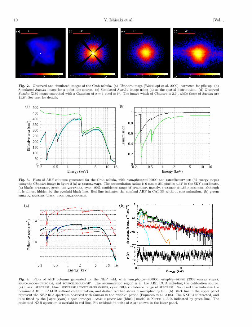
The NEP field is an archetypal “blank field”, where noX-ray bright objects exist. In such a region, the X-raybackground, including both the extra-galactic (Brandt &Hasinger 2005) and the Galactic components (Snowdenet al. 1995), is the dominant X-ray source. The X-raybackground can be treated as almost uniform distribu-tion, hence we tested the uniform-sky ARF generated byxissimarfgen in this field.We created an ARF assuming a uniform distribution

for the source from a circular region with a radius of 20′

(see caption of figure 4 for details of the parameters), andfitted the observed spectrum with it. In figure 4 (a), theeffective area, specresp, of the obtained ARF is displayedin comparison with that for a point source. One can seethat the effective area is relatively smaller in the higherenergy band (>∼ 7 keV), due to the vignetting effect of theXRT. After subtracting the NXB contribution estimatedusing the night Earth database (§ 5.2), the spectrum canbe well fitted with a power-law model representing theCXB and one or two thin-thermal plasma models repre-senting local Galactic thermal components, as shown infigure 4 (b). The photon index and the surface brightnessof the power-law component are consistent with the pa-rameters reported so far (Gendreau et al. 1995; Kushinoet al. 2002). See Fujimoto et al. (2006) for the details ofthe analysis. This result demonstrates that xissimarfgenproperly generates the ARF for the uniform-sky emission.

6.3. Abell 1060 Cluster of Galaxies

Finally, we present an example of the Abell 1060 clusterof galaxies observed with Suzaku. Scientific results will bepublished by K. Sato et al. in preparation. Abell 1060 is acircular and nearly isothermal (∼3 keV) cluster of galaxies(Tamura et al. 2000; Furusho et al. 2001; Hayakawa etal. 2004; Hayakawa et al. 2006) and is suitable for testingthe ARF for extended sources. There were two pointingsperformed with Suzaku at the central region and the ∼20′ east offset region, as shown in figure 5 (a). Theseobservations were conducted at the end of November 2005,when the XIS contamination was already significant andwas starting to saturate.The observed spectrum is assumed to contain (a) thin

thermal plasma emission from the intra cluster medium(ICM), (b) local Galactic emission, (c) CXB, and (d)NXB. We can estimate (d) using the night Earthdatabase mentioned in § 5.2, and can subtract it from theobserved spectrum. As demonstrated in § 6.2, the spec-trum of (b) can be represented by the (apec + apec) modelwith 1 solar abundance, and that of (c) has a shape ofabsorbed power-law with Γ ≃ 1.4. However, we cannot

10 Y. Ishisaki et al. [Vol. ,

Fig. 2. Observed and simulated images of the Crab nebula. (a) Chandra image (Weisskopf et al. 2000), corrected for pile-up. (b)Simulated Suzaku image for a point-like source. (c) Simulated Suzaku image using (a) as the spatial distribution. (d) ObservedSuzaku XIS0 image smoothed with a Gaussian of σ = 4 pixel ≃ 4′′. The image width of Chandra is 2.9′, while those of Suzaku are11.6′. See text for details.

0

50

100

150

200

250

300

350

400

450

500

0.2 0.5 1 2 5 10 16

Eff

ectiv

e ar

ea (

cm2 )

Energy (keV)

(a)

0

0.2

0.4

0.6

0.8

1

0.2 0.5 1 2 5 10 16

Tra

nsm

issi

on

Energy (keV)

(b)

Fig. 3. Plots of ARF columns generated for the Crab nebula, with num photon=100000 and estepfile=sparse (55 energy steps)using the Chandra image in figure 2 (a) as source image. The accumulation radius is 6 mm = 250 pixel ≃ 4.34′ in the SKY coordinate.(a) black: specresp, green: xrt effarea, cyan: 90% confidence range of specresp, namely, specresp± 1.65× resperr, althoughit is almost hidden by the overlaid black line. Red line indicates the nominal ARF in CALDB without contamination. (b) green:shield transmis, black: contami transmis.

Fig. 4. Plots of ARF columns generated for the NEP field, with num photon=400000, estepfile=dense (2303 energy steps),source mode=uniform, and source rmax=20′. The accumulation region is all the XIS1 CCD including the calibration source.(a) black: specresp, blue: specresp /contami transmis, cyan: 90% confidence range of specresp. Solid red line indicates thenominal ARF in CALDB without contamination, and dashed red line shows it multiplied by 0.1. (b) Black line in the upper panelrepresent the NEP field spectrum observed with Suzaku in the “stable” period (Fujimoto et al. 2006). The NXB is subtracted, andit is fitted by the [ apec (cyan) + apec (orange) +wabs × power-law (blue) ] model in Xspec 11.3.2t indicated by green line. Theestimated NXB spectrum is overlaid in red line. Fit residuals in units of σ are shown in the lower panel.

No. ] Suzaku XRT/XIS Simulator & ARF Generator 11

fit the observed spectrum directly by a sum of (a) + (b)+ (c), because the spatial distribution of these three aredifferent on the sky, as described in § 4.1.We therefore adopted the following method for the spec-

tral analysis of Abell 1060. We extracted several spectrafrom annular regions centered on the cluster core, andhere we show two samples of the innermost region at theprojected radius of 0–2′ from the central observation, andthe outermost region of 17–27′ from the offset observation,as representatives. We generated two different ARFs foreach spectrum, Au(Ei) and Ab(Ei), which respectivelyassume the uniform-sky emission and the ICM surfacebrightness profile obeying an analytical model obtainedwith the XMM-Newton data.As described in § 4.1, it is important that the assumed

spatial distribution on the sky well agrees with the actualdata in the calculation of the ARF response. We thereforecompared the observed images with the simulated ones infigure 5 (b) and (c). The 1–4 keV energy range was chosenso that the distortion of the image due to the XIS contam-ination and the XRT vignetting was not severe. In thisenergy range, the Galactic component (b) is almost negli-gible, whereas the CXB and NXB components cannot beneglected especially in the offset observation. The NXBcomponent (red line) is estimated from the night Earthdatabase. A small ACTY (= DETY−1 for XIS0, see fig-ure 8) dependence of the NXB intensity is seen, reflectingthe dwell time at the frame-store region of the CCD. TheCXB component (blue line) is estimated by the xissimsimulation, assuming the uniform sky and the previousASCA results of the CXB intensity (Kushino et al. 2002).The vignetting effect is seen in the CXB counts, hencethe count rate slightly drops at the CCD rim. After thesubtraction of the estimated CXB and NXB components,the observed distribution of the cluster (black crosses) isfairly well reproduced by the xissim simulation of the clus-ter emission (green line), although a small asymmetry isobserved for the real cluster in the central observation.Figures 6 (a)–(d) show the latter kind of ARFs, Ab(Ei),

for both regions. Figures 6 (a) and (b) correspond tothe extraction regions of 0–2′ and 17–27′, respectively, inthe DET coordinate, and the calibration source area (top-left and bottom-right for XIS1) is also excluded in (b).Although the accumulation area is smaller for (a) than(b), the calculated effective area is much larger for (a)than (b) as seen in figure 6 (c), plotted in black and redlines, respectively, due to the assumed surface brightnessprofile. One can see the position dependence of the XIScontamination (thinner towards the CCD edge) is treatedappropriately as seen in figure 6 (d).Denoting the spectra of (a), (b), (c), and (d) as

M icm(Ei), M gal(Ei), M cxb(Ei), and Mnxb(PI j), the ob-served spectrum can be expressed by a sum of,

Ab⊗M icm +Au⊗M gal +Au⊗M cxb +Mnxb, (5)

where the operator ⊗ denotes the transformation definedby eq. (1). It is known that the CXB spectrum, M cxb,is fairly constant over the sky except for difference inthe neutral hydrogen column density, NH, for absorption,

whereas the local Galactic emission, M gal, may vary fromfield to field by more than an order of magnitude (Kushinoet al. 2002).Considering this situation, we assumed a power-law

spectrum for the CXB with the values by Kushino etal. (2002), Γ=1.4 and SX=5.97×10−8 erg cm−2 s−1 sr−1

(2–10 keV),10 measured with the ASCA GIS (Ohashi etal. 1996; Makishima et al. 1996). The neutral hydro-gen column density was fixed to NH = 4.9× 1020 cm−2

(Dickey & Lockman 1990). We calculated the estimatedcontribution of the CXB, Au⊗M cxb, using the fake com-mand in Xspec. This contribution for each region isindicated by blue crosses in figures 7 (a) and (b) forXIS1. We subtracted the CXB contribution from theobserved spectrum as well as the estimated NXB spec-trum. The XIS1 (red) and FI (XIS0+XIS2+XIS3; black)spectra in figures 7 (a) and (b) denote those after theCXB and NXB subtraction. We then fitted the XIS1and FI spectra simultaneously for the offset observation,where the Galactic component (b) is prominent, with the[ apec (cyan)+ apec (orange)+ phabs × vapec (magenta) ]model, using the ARF response, Ab(Ei).In a strict sense, using Ab for the component (b) is not

correct, which should be Au instead. We made this choicedue to the limitation of the Xspec v11 (§ 4.1), however,it does not matter practically if we only notice the shapeof the spectrum. The absolute surface brightness of theGalactic component was evaluated separately using theXspec fake command and the Au response. We thenfitted the central region, fixing the shape of the Galacticcomponent, but with its normalization scaled so that thesurface brightness is preserved between the two differentsky regions. Xspec v12 can handle this situation morestraightforwardly.The released RMF, ae xi[0-3] 20060213.rmf, was

used for the spectral analysis. The ARFs were gener-ated by xissimarfgen, and were convolved with the RMFsand added for three FI sensors, using the marfrmf andaddrmf tasks in Ftools. As for the photon statisticsof the simulation, limit mode=mixed was chosen withnum photon=100000 and accuracy=0.005. As seen in fig-ures 7 (a) and (b), both the observed spectra can be wellfitted by one temperature plasma emission model for ICM,and (apec + apec) model with 1 solar abundance for thelocal Galactic emission. The surface brightness and thespectral shape of the Galactic emission is kept constantbetween both regions. This is confirmed by the fact theratio of the Galactic components to the CXB is almostequal between figures 7 (a) and (b). Note that the fit ap-pears equally good to the BI (XIS1) and FI sensors, whichare different in the thickness of the contamination. Sofar, it has been confirmed that the temperature for eachring derived from the spectral fitting with this methodis quite consistent with the previous results with XMM-Newton and Chandra (Hayakawa et al. 2004; Hayakawa

10 This value is taken from table 3 of Kushino et al. (2002), forthe integrated spectrum with source elimination brighter thanS0 =2×10−13 erg cm−2 s−1 (2–10 keV) in the GIS filed of viewwith Γ = 1.4 (fix) and the nominal NXB level (0%).

12 Y. Ishisaki et al. [Vol. ,

et al. 2006). See K. Sato et al. in preparation for detailsof the results.

7. Summary

• We have developed a Monte-Carlo simulator of theSuzaku XRT/XIS system taking into account fullcalibration results.

• We adopted the ANL platform that provides usa flexible and comprehensive environment for theSuzaku software production.

• There is a dedicated task named mkphlist whichgenerates a photon file to feed to the simulator.

• The task xissim reads the photon file, and con-ducts the instrumental simulation using the XRTray-tracing library and the RMF of the XIS, andgenerates an event file, which is consistent withthat for real observation, so that users can analyzethe simulated data in the same manner as real data.

• The simulator-based ARF generator is namedxissimarfgen, which can compute up to 200 ARFscorresponding to different accumulation regions bya single batch of simulations.

• The combination of xissim and xissimarfgen enablesusers to analyze spatially extended and spectro-scopically complex celestial sources.

• Since one of the Suzaku’s unique features is thelow and stable particle background, these simu-lators are crucial for producing scientific resultswith low signal-to-noise data from extended sources.

• The latest public version is 2006-08-26, which willbe included in the next official release of the SuzakuFtools scheduled in late 2006.

Thanks are given to the referee, Dr. K. Arnaud, foruseful comments which improved the original manuscript.We express sincerely thanks to H. Honda for early stagework on the ASCA ANL, and SimASCA. We also showR. L. Fink our appreciation for early stage work on thexrrt ray-tracing library. We acknowledge to L. Angeliniand I. Harrus for useful discussion on the CALDB file for-mat. We thank K. Mori to provide us a Chandra imageof the Crab nebula corrected for pile-up photons. Wealso acknowledge D. McCammon, R. Smith, Y. Takei,C. Matsumoto, and N. Ota for testing and giving valu-able comments on the xissim and xissimarfgen tasks. Partof this work was financially supported by the Ministryof Education, Culture, Sports, Science and Technology ofJapan, Grant-in-Aid for Scientific Research No. 14079103,15001002.

Table 3. Summary of XIS coordinate column information.

Column Name Min ∗ Max † Origin ‡ Pixel Size §

segment 0 3 – –rawx/y 0 255/1023 – 0.024 mmactx/y 0 1023 – 0.024 mmdetx/y 1 1024 512.5 0.024 mmfocx/y 1 1536 768.5 0.024 mm

x/y 1 ‖ 1536 ‖ 768.5 0.0002895 deg ♯

∗ TLMINn keywords in the event file.† TLMAXn keywords in the event file.‡ TCRPXn keywords in the event file.§ TCDLTn keywords in the event file.‖ Default image region. X/Y values can be outside of the region.♯ Angular scale at the center. Outer pixels are slightly differentdue to the tangential projection.

Table 4. Summary of XIS alignment information

Item Ideal ValueFocal length 4750 mmOptical axis location in DET (512.5, 512.5)Size of the DET pixel 0.024 mm/pixelOffsets between DET and FOC (0.0, 0.0)Roll angle between DET and FOC 0.0 degAlignment matrix for FOC → SKY ∗ 3× 3 identity matrix

∗ Alignment matrix is common to all sensors.

Appendix 1. Definition of the Coordinates

The following coordinates are defined to describe eventlocations in the telemetry, on the detector, or on the sky.

RAW coordinates: Original digitized values in thetelemetry to identify the pixels of the events. This maynot reflect physical locations of the pixels on the sensor.For example, XIS RAWX (or RAWY) coordinate will havevalues from 0 to 255 (or 1023) on each CCD segment.Each of the four XIS sensors has a single CCD chip, anda single chip is divided into four segments.

ACT coordinates: The ACTX/Y values are definedto represent actual pixel locations in the CCD chips.ACTX/Y will take 0 to 1023 to denote the 1024 ×1024 pixels in the chip. The XIS RAW to ACT conver-sion depends on the observation modes (such as WindowOptions) and will require housekeeping information. TheXIS ACT coordinate is defined by looking down on thesensors, hence the ACTX/Y to DETX/Y conversion needsa flip in the Y-direction.

DET coordinates: Physical positions of the pixelswithin each sensor, XIS0–3. Misalignments between thesensors are not taken into account. The DETX/Y coordi-nate are defined by looking up the sensor, such that thespacecraft (S/C) +Y direction becomes the −DETY di-rection (the same convention as with ASCA ). The S/CZ-axis points in the telescope direction, and +Y direc-tion is toward the solar paddle. For XIS, the DETX andDETY values take 1 to 1024.

FOC coordinates: Focal plane coordinate common to

No. ] Suzaku XRT/XIS Simulator & ARF Generator 13

Fig. 5. (a) Observed Abell 1060 image combined for the central and offset pointings obtained with XIS0 in the 1–4 keV energyrange. The image is smoothed with σ=16 pixel ≃ 17′′ Gaussian, and the estimated NXB and CXB components are subtracted. Theexposure time is corrected, but vignetting is not corrected. Directions of DETX/Y axes are indicated in the figure. (b) Comparisonof the observed and the simulated images (1–4 keV) projected to the DETY axis in the offset pointing. The green line shows thesimulated distribution by xissim assuming an analytical model (double-β model) obtained with XMM-Newton, and the kT =3.4 keVvapec model spectrum. The blue and red lines show the estimated CXB and NXB distribution, respectively. The black crosses showthe observed distribution after subtracting the CXB and NXB components. (c) Same as (b), but for the central observation.

Fig. 6. Plots of the XIS1 ARFs for the Abell 1060 cluster of galaxies calculated with limit mode=mixed, num photon=100000,accuracy=0.005, and estepfile=dense. (a) The primary extension image in DET coordinate (1024×1024) for the central observationat the projected radius of r < 2′. (b) Same as (a) but for the offset observation at the projected radius of 17′ < r < 27′. (c) Thespecresp columns for the central (black) and offset (red) observations plotted against energy. The 90% confidence range for eachARF is indicated by cyan or green lines, respectively. (d) The contami transmis columns for the central (black) and offset (red)observations.

(a) (b)

Fig. 7. Example spectra of the Abell 1060 cluster of galaxies, (a) for the central observation, (b) for the offset observation. In bothfigures, red or black crosses represent the observed spectrum with the XIS1 (BI) or XIS0+XIS2+XIS3 (FI) sensor(s), respectively,for the upper panels, and the fit residuals for the lower panels. The estimated CXB + NXB spectrum has been subtracted fromeach observed spectrum, and the estimated CXB spectra for XIS1 are indicated by blue crosses. The spectra are fitted by the[ apec (cyan) + apec (orange) + phabs × vapec (magenta) ] model in Xspec 11.3.2t indicated by green line for XIS1 and yellow linefor the FI sensors. The model components are only plotted for the XIS1 spectrum.

14 Y. Ishisaki et al. [Vol. ,

A

B

C

D

ACTY

ACTX

RAWY

RA

WX

XIS-1 (BI)

ABD

ACTX

AC

TY

RA

WY

RAWX

C

XIS-3

A

B

C

D

ACTX

ACTY

RAWY

RA

WX

XIS-2

ABD

ACTX

AC

TY

XIS-0

RA

WY

RAWX

C

Calibration

Source

DETY

DETX

S/C X

S/C Y

Fig. 8. Relations between RAWX/Y, ACTX/Y, DETX/Y among the four XIS sensors. The coordinate are defined looking upfrom the XIS toward the XRT.

all the sensors. Misalignments between the sensors aretaken into account so that the FOC images of differentsensors can be superposed. The origin of the FOC coor-dinate corresponds to the XIS nominal position for point-ing observations. FOC is calculated from DET by lin-ear transformation to represent the instrumental misalign-ment, i.e., the offset and the roll angle.

SKY coordinate: Positions of the events on the sky.For each XIS event, the equatorial coordinate of the pixelcenter projected on a tangential plane are given. Theaberration correction due to parallax (i.e., the revolutionof the Earth around the Sun) is also considered.

XRT coordinate: This is given by (XRTX, XRTY) inmm on the focal plane, or (θ, φ) corresponding to theoffset angle (′) and the azimuth angle (◦) with respect tothe optical axis of each XRT. The location of the opticalaxis on the DET coordinate is defined so that effectivearea of the XRT is maximized.

The RAW, ACT, DET, FOC and SKY coordinate arewritten in the Suzaku XIS event files. Relations betweenRAWX/Y, ACTX/Y, DETX/Y among the four XIS sen-sors are summarized in figure 8. The DETX/Y pixel sizescorrespond to the physical pixel size of the XIS CCD,while the X/Y pixel size corresponds to the angular scaleof a single CCD pixel at the reference pixel. To allow rota-tion of the image and some shift of the pointing directionduring the observation, the X/Y range is taken slightly

bigger than√2× 1024. The minimum value, maximum

value, origin of the coordinate (reference pixel location),and pixel size are summarized in table 3.There is a file called teldef (namely, telescope definition)

for each sensor. In the primary header of each teldef file,alignment data for the individual sensors (DET→FOC,FOC→SKY, and DET→XRT) are given. The alignmentparameters in the teldef file are summarized in table 4. Inthe extensions of the teldef files, sensor-dependent addi-tional calibration information may be written. For exam-ple, the 1st extension of the XRS teldef file has measuredpositions and sizes of the XRS pixels.In this scheme, the conversion from RAW to DET does

not depend on the misalignments between the sensors.Therefore, DETX/Y, as well as RAWX/Y, can be writ-

ten in the event files without having the calibration infor-mation. The DET to FOC conversion requires the sensormisalignment data. The conversion from FOC to SKYis made using the satellite Z-Y-Z Euler angles (ea1, ea2,ea3) in the attitude file and the 3×3 alignment matrixgiven in the teldef file. One must be careful because thisconversion is dependent on the observation date and di-rection due to the parallax (aberration) correction. Themagnitude of the correction is about ±20.5′′ at maximum.All the conversions between these coordinates are sup-

plied in the form of the C functions in the astetool li-brary. These functions make use of the information givenby the teldef file, and it is strongly recommended to usethem for the coordinate conversions. They are built onthe ISAS-made mission-independent library named at-

Functions, which includes basic routines to handle 3-dimensional vectors and rotation matrices. There is alsoa frontend of the coordinate conversions in the SuzakuFtools, named aecoordcalc.

Appendix 2. Structures & Parameters

A.2.1. mkphlist

The mkphlist task consists of three ANL modules aslisted in table 5. The SimASTE Root (we will omitSimASTE hereafter in the main text) module is a rootmodule for the Suzaku simulators, that handles initial-ization of random numbers and common CALDB files.The PhotonGen module generates photons according tothe parameters set by a user, and caches the photon pa-rameters in an internal storage area called BNK (Ozaki etal. 2006). The PhotonFitsWrite module retrieves the pho-ton data from the BNK and writes the data to the photonfile. By splitting these functions into dedicated ANL mod-ules, it is easier to understand the structure of the task,and furthermore we can share the modules among severaltasks. For example, the Root module is used for all theSimASTE tasks, and the PhotonGen modules is sharedwith xissim.The parameters of the PhotonGen module (table 5) is

classified into the following five groups: (1) to determinethe X-ray flux, photon flux, flux emin, flux emax, and geo-

metrical area; (2) to determine the spectral shape of inci-

No. ] Suzaku XRT/XIS Simulator & ARF Generator 15

dent X-rays, spec mode, qdp spec file, and energy; (3) todetermine the spatial distribution on the sky, image mode,ra, dec, sky r min, sky r max, fits image file; (4) to deter-mine the photon arrival time to be equal or random inter-val steps, time mode; (5) to determine how many photonsare to be generated, limit mode, nphoton, and exposure.

A.2.2. xissim

Table 6 summarizes the ANL modules and major pa-rameters for xissim. It consist of eight modules, the firsttwo modules of which are common to mkphlist.In the Root module, the simulation mode, instrume,

teldef, and leapfile parameters are added (which are ig-nored in mkphlist) when compared with table 5. The sim-

ulation mode parameter determines the default mode ofthe simulation, and the two defined modes are discardand weight. In the discard mode, each absorbed pho-ton is discarded, for example, by absorption in the XRTthermal shield. In contrast, the weight of the photon isdecreased by multiplying the transmission probability ofthe thermal shield in the weight mode. The final valueof the weight is written to the weight column of theoutput event file. This feature enables efficient simulationwhen most of photons disappear during the simulation,however one needs to use care in the handling of the simu-lation results. The default simulation mode is discard forxissim, whereas simulation mode=weight for xissimarf-gen to treat the thermal shield transmission separately(§ 4.2).The PhotonGen module enables on-the-fly photon gen-

eration without input photon files, and is usually deac-tivated (enable photongen=no). The same parameters intable 5 are usable in this mode. The PhotonRead mod-ule reads up to eight photon files, as well as the GTI fileand the attitude file, and puts the photon data (ra, dec,photon time, photon energy) and the Euler anglesat photon time into BNK. By mixing multiple photonfiles, it is capable of simulating an observation, e.g. hotand widely extended emission from a cluster of galaxieswith cool emission from the core region.The ECStoXRTIN module takes care of the pre-XRT

component. It retrieves the photon data and the Eulerangles, and converts the photon positions into (θ, φ). Theparallax (aberration) correction and the cos θ effect arealso considered here. XRTsim conducts the ray-tracingby calling the xrrt library, and the XRTOUTtoDET com-pute the detector position hit by the photon. XISRMFsimsimulates the XIS using the RMF, and XISevtFitsWritewrite the final output (table 9) into the event file.

A.2.3. xissimarfgen

Table 7 summarizes the structure and parameters ofxissimarfgen. It consists of five ANL modules, and threeout of which are common to xissim. The two dedi-cated modules for xissimarfgen are XISarfPhotonGen andXISarfBuild, and they closely cooperate to calculate andgenerate the resultant ARF(s) by driving the XRT partof the simulator, XRTsim and XRTOUTtoDET.In table 7, parameters of common modules to xissim

Table 5. Structure and parameters of mkphlist.

Module/Parameter ∗ DescriptionSimASTE Root

(rand seed) random number seed(rand skip) random number skip count

SimASTE PhotonGenphoton flux photon flux (photons cm−2 s−1)flux emin lower energy (keV) for photon flux

flux emax upper energy (keV) for photon flux

geometrical area XRT geometrical area (cm2)spec mode 0:qdp-spec, 1:monochromeqdp spec file qdp spectral file for spec mode=0energy energy (keV) for spec mode=1image mode 0:FITS-image, 1:point, 2:uniformra, dec ra, dec (◦) for image mode=1 or 2sky r min min radius (′) for image mode=2sky r max max radius (′) for image mode=2fits image file image FITS file for image mode=1time mode 0:constant, 1:Poissonlimit mode 0:number of photon, 1:exposure timenphoton number of photon for limit mode=0exposure exposure time (s) for limit mode=1

SimASTE PhotonFitsWriteoutfile output photon file name

∗ Parameters in parentheses are hidden parameters.

are omitted, although the simulation mode parameter isset to weight as mentioned in A.2.2. We can categorizethem as follows: (a) to specify the spatial distribution ofthe celestial target on the sky, source mode, source image,etc; (b) to specify the accumulation region of the de-tected events and corresponding output ARF names, re-gion mode, num region, regfileN , detmask, and arffileN ; (c)to specify the photon statistics at each energy, limit mode,num photon, and accuracy; (d) to specify the energy stepto calculate the detection efficiency, rmffile and estepfile;(e) to specify the observation date and the satellite Eulerangles, gtifile, date obs, attitude, ea1, ea2, and ea3; (f) tospecify other calibration information or simulation modesor reference of the SKY coordinate, contamifile, aberration,aperture cosine, pointing, ref alpha, ref delta, and ref roll.Groups (e) and (f) parameters are similar to xissim.Group (a) parameters determine the spatial distribu-

tion of the target on the sky, and one can specify anarbitrary FITS image in the SKY or DET coordinate(source mode=skyfits/detfits). Pixels with negativevalues are treated as zero in the image. Otherwise, alocation of a point source can be set in the equato-rial coordinate in J2000, or SKY- or DET-coordinate(source mode=j2000/skyxy/detxy). In addition, auniform-sky emission with respect to the XRT coordinatecan be selected (source mode=uniform). When the FITSimage or the location of the point source is supplied in theDET coordinate, its position on the sky will be affectedby the wobbling of the spacecraft, hence it is not recom-mended to use with the attitude file.Note that one must specify skyref to use SKY co-

ordinates. When source mode=skyfits, skyref is au-tomatically read from the FITS header keywords. As

16 Y. Ishisaki et al. [Vol. ,

Table 6. Structure and parameters of xissim.

Module/Parameter ∗ DescriptionSimASTE Root

instrume instrument (xis0,xis1,xis2,xis3)(simulation mode) 0:discard, 1:weight(rand seed) random number seed(rand skip) random number skip count(teldef) teldef file name(leapfile) leap second file

SimASTE PhotonGen †

(enable photongen) enable on-the-fly photon generationSimASTE PhotonRead

infileN input photon file(s) up to N = 8(gtifile) name of the GTI file or none(date obs) observation start for gtifile=none(date end) observation end for gtifile=none(attitude) name of the attitude file or noneea1, ea2, ea3 Euler angles for attitude=none(pointing) pointing type, auto or userref alpha skyref ra (◦) for pointing=userref delta skyref dec (◦) for pointing=user(ref roll) skyref roll (◦) for pointing=user

SimASTE ECStoXRTIN(aperture cosine) consider aperture decrease by cosθ(aberration) ‡ enable the aberration correction

SimASTE XRTsim(shieldfile) XRT thermal shield transmission file(mirrorfile) XRT mirror geometry file(reflectfile) XRT surface reflectivity file(backproffile) XRT backside scatter profile file

SimASTE XRTOUTtoDETSimASTE XISRMFsim

xis rmffile XIS RMF name(aberration) ‡ enable the aberration correction(xis contamifile) XIS contamination file or none(xis efficiency) multiply XIS effciency or not(xis chip select) discard events fallen outside of CCD

SimASTE XISevtFitsWriteoutfile output event file name

∗ Parameters in parentheses are hidden parameters.† See table 5 for rest of parameters when enable photongen=yes.‡ The aberration parameter is read in two modules.

long as the WCS (world coordinate system; Greisen& Calabretta 2002; Calabretta & Greisen 2002) key-words are correctly assigned, one may use an image forsource image. When source mode=skyxy, things are a lit-tle complicated. If pointing=user, the ref alpha, ref delta,and ref roll parameters are utilized for skyref. If point-

ing=auto, which is the default, skyref is read fromthe header keywords of the attitude file, ra nom anddec nom, and roll of skyref is always set to 0◦, unlessattitude=none. If pointing=auto and attitude=none,skyref is calculated from the specified Euler angles, ea1,ea2, and ea3, as ra= ea1, dec=90◦−ea2, and roll=0◦.Group (b) parameters decide the accumulation re-

gion(s) of the detected events. The num region parameterspecify the number of regions to be considered in the ARFcalculation. Up to 200 regions may be specified in a sin-gle batch of simulations. One may specify FITS image(s)

Table 7. Structure and parameters of xissimarfgen.

Module/Parameter Description

SimASTE Root †

SimASTE XISarfPhotonGen(pointing) pointing type, auto or userref alpha skyref ra (◦) for pointing=userref delta skyref dec (◦) for pointing=user(ref roll) skyref roll (◦) for pointing=usersource mode skyfits,detfits,

j2000,skyxy,detxy,uniformsource image FITS image for source mode=*fitssource ra ra (◦) for source mode=j2000source dec dec (◦) for source mode=j2000source x x (pixel) for source mode=*xysource y y (pixel) for source mode=*xysource rmin min θ (′) for source mode=uniformsource rmax max θ (′) for source mode=uniformregion mode skyfits,detfits,skyreg,detregnum region number of accumulation regionsregfileN region file #N , N=1∼ num region

arffileN output ARF #N , N=1∼ num region

detmask mask image in DET coord. or nonelimit mode mixed,num photon,accuracynum photon number of photons for each energyaccuracy calculation accuracy for each energygtifile name of the GTI file or nonedate obs date of observation for gtifile=noneattitude name of the attitude file or noneea1, ea2, ea3 Euler angles for attitude=nonermffile RMF to retrieve energy binestepfile E step file or dense,medium,sparse(contamifile) XIS contamination file or none(aberration) enable the aberration correction(aperture cosine) consider aperture decrease by cosθ

SimASTE XRTsim †

SimASTE XRTOUTtoDETSimASTE XISarfBuild

† See table 6 for other parameters.

or DS9-style region file(s) in SKY- or DET-coordinate(region mode=skyfits/detfits/skyreg/detreg). Insupplying a FITS image, an unbinned image (1536×1536for SKY, 1024× 1024 for DET) is needed to avoid am-biguity. The skyref is adopted in the same way whensource mode=skyxy, and the header keywords in theFITS image(s) are always ignored. One may optionally setthe detmask parameter to specify a mask image in DETor ACT coordinates, which is automatically judged by thectype1 and ctype2 header keywords. The detmask im-age is commonly applied to the all of the specified regions,so that this feature is useful in excluding the calibrationsource regions, bad CCD columns, and hot/flickering pix-els from the accumulation regions.In supplying a FITS image with the regfileN parame-

ter, the pixel values are interpreted as follows. After thesimulation of each photon, the pixel location on the im-age is determined. If the pixel value is zero or negative,the photon is discarded as a non-detection. If it is posi-tive, the weight of the photon is multiplied by the pixelvalue. Therefore, one should normally supply a binary

No. ] Suzaku XRT/XIS Simulator & ARF Generator 17

Table 8. List of columns in the photon file.

Column Name Format∗ Unit Descriptionphoton time 1d s arrival timephoton energy 1e keV X-ray energyra 1e deg right ascension of incidencedec 1e deg declination of incidence

∗ The column format in FITS convention. ‘1d’ is a double preci-sion floating point, and ‘1e’ is a single precision floating point.

(0/1) mask image, while a gray-scale image can representnon-uniform exposure areas.Group (c) parameters specify conditions for the

photon statistics at each simulation energy. Whenlimit mode=num photon, num photon count of pho-tons are generated at each simulation energy, re-gardless of the number of detected photons. Whenlimit mode=accuracy, photons are generated until therelative error of the detection efficiency becomes lessthan the accuracy parameter for all the accumulation re-gions. The relative error is calculated by eq. (4). It maytake so many photons when the detection efficiency isquite low in this mode that it is recommended to specifylimit mode=mixed, in which it generates photons until ei-ther of the two conditions is fulfilled. If num photon=0 oraccuracy=0 in limit mode=mixed, the former or the latteris ignored, respectively.Group (e) parameters are utilized to specify the simu-

lation energy step. The XIS RMF specified by the rmf-

file parameter is only used to retrieve the energy bin,Ei, for the output ARF(s), so that an out-of-date RMFmay do so far as the energy bin is the same. The es-

tepfile parameter should be one of the preset keywordsfull/dense/medium/sparse, or point to a file that con-tains three decimal numbers, Emin, Emax, Ebin, on eachline. When estepfile=full, the simulation is conductedat every RMF energy bin (m = 7900 energy steps), ran-domizing each photon energy within a ±1 eV range, whichcan result in a very long computation time. When estep-

file=dense/medium/sparse, the simulation is conductedat built-in fixed energies of 2303/157/55 steps, respec-tively. These energies are optimized considering the edgeenergies, so that even estepfile=sparse can produce anacceptable quality ARF for the scientific spectral fittinganalysis with a featureless and moderate-statistics spec-trum.

Appendix 3. Output File Formats

A.3.1. Output of mkphlist

Table 8 denotes the format of the output photon filefrom mkphlist, which is also the input to xissim. Thetime, energy, and direction of the incident photons arecontained in the photon time, photon energy, and(ra, dec) columns, respectivly. This file is basically mis-sion independent, except for the geomarea keyword inthe FITS header, which contains the geometrical area ofXRT (cm2) specified by the geometrical area parameter ofmkphlist.

Table 9. List of columns in the simulated event file.

Column Name Format∗ Unit Description1st extension ’events’time 1d s detected timepha 1i chan pulse height (= pi)pi 1i chan pulse invariantstatus 1i status flags (= 0)grade 1i event grade (= 0)segment 1i CCD segment idrawx 1i pixel RAW coordinate x valuerawy 1i pixel RAW coordinate y valueactx 1i pixel ACT coordinate x valueacty 1i pixel ACT coordinate y valuedetx 1i pixel DET coordinate x valuedety 1i pixel DET coordinate y valuefocx 1i pixel FOC coordinate x valuefocy 1i pixel FOC coordinate y valuex 1i pixel SKY coordinate x valuey 1i pixel SKY coordinate y valuexisx 1e pixel floating point value of detxxisy 1e pixel floating point value of detyweight 1e weight of the eventphoton time 1d s copy of input photon filephoton energy 1d keV copy of input photon filera 1d deg copy of input photon filedec 1d deg copy of input photon file2nd extension ’gti’start 1d s start of valid timestop 1d s stop of valid time

∗ The column format in FITS convention. ‘1d’ is a double preci-sion floating point, ‘1e’ is a single precision floating point, ‘1i’ isa 16-bit integer.

Table 10. List of columns in the generated ARF.

Column Name Format∗ Unit DescriptionPrimary extension ’wmap’[image] 1d count image of detected events1st extension ’specresp’energ lo 1e keV lower energy binenerg hi 1e keV higher energy binspecresp 1e cm2 computed effective arearesperr 1e cm2 error of specrespresprerr 1e relative error of specrespxrt effarea 1e cm2 XRT only effective areashield transmis 1e thermal shield transmissioncontami transmis 1e contamination transmissionindex 1j index of simulated energys 1e interpolation coefficientt 1e interpolation coefficientinput 1e count number of input photonsdetect 1e count sum of detected eventsweisum 1e count weighted sum of eventsrelerr 1e relative error of detect

∗ The column format in FITS convention. ‘1d’ is a double preci-sion floating point, ‘1e’ is a single precision floating point, ‘1j’ isa 32-bit integer.

18 Y. Ishisaki et al. [Vol. ,

Table 11. List of special header keywords in the output ARF.

Keyword Name Descriptiongeomarea geometrical area of XRT (cm2)teldef teldef file nameleapfile leap second file namecreator xissimarfgen credit and versionsource ratio reg source image ratio inside selected regionmask ratio ccd detmask ratio in the whole CCD areamask ratio reg detmask ratio inside selected regionn photon number of input photons generatedn detect number of events detected ∗

n weisum weighted sum of events detected ∗

randseed random number seed, = rand seed

randskip random number skip count, = rand skip

randngen number of random numbers generated

∗ Events fallen on a pixel with a positive value for at least one ofthe accumulation regions are treated as “detection”, here.

A.3.2. Output of xissim

Table 9 denotes the format of the output event filefrom xissim. The output is a standard FITS event filewith events and gti extensions, plus information on thefaked input photons. If the attitude file is given, posi-tion on the sky (x and y) is corrected for the wobbling ofthe spacecraft, as well as the parallax (aberration). Forthe calculation of the x and y columns, the sky reference(skyref ) of (RAref , DEC ref , Roll ref) must be specified byusers as the parameters of ref alpha, ref delta, and ref roll,although ref roll is hidden and usually set to 0. The (x, y)positions have a one-to-one correspondence to sky direc-tions, however these direction do not necessarily coincidewith the incident direction of the photon, (ra, dec), dueto blurring by the PSF of the XRT.

A.3.3. Output of xissimarfgen

Table 10 summarizes the format of the output ARF gen-erated by xissimarfgen. In comparison with the minimumset of the ARF (energ lo, energ hi, and specrespcolumns), it has several additional columns and the pri-mary image extension to record the information of thesimulation. All of the parameters for xissimarfgen arewritten in the history of the output ARF, and several im-portant simulation parameters and results are written tothe FITS header keywords listed in table 11.The energ lo and energ hi columns, both in units

of keV, are copied from the input RMF, and xissimarf-

gen assumes Ei = (energ lo+energ hi) / 2 and ∆Ei =energ hi− energ lo for the i-th row (i = 1 ∼ m, andm= 7900 for the nominal RMF). The specresp columnholds the final result of the detection efficiency times thegeometrical area, S A(Ei), in unit of cm2. The value of S(cm2) assumed in the calculation is written to the FITSheader keyword of geomarea (table 11). The resperrand resprerr columns hold the absolute and relativeerrors, respectively, estimated for the specresp column,i.e. resperr = resprerr × specresp. Details are de-scribed in § 4.2 for the xrt effarea, shield transmis,and contami transmis columns.

The input, detect, and weisum columns hold inter-polated values of Nin, Ndet, and Nw, respectively. Theweisum represents the weighted sum of events, and isusually equal to detect unless one supplies a gray-scaleregion file. The relerr is an interpolated value of therelative error calculated by eq. (4). The coefficients of theinterpolation, si and ti, are defined as,

V (Ei) = si V (E′indexi

)+ti V (E′indexi+1), (A1)

si = (E′indexi+1 −Ei) / (E

′indexi+1 −E′

indexi), (A2)

ti = (Ei −E′indexi

) / (E′indexi+1 −E′

indexi), (A3)

where E′indexi

denotes the simulated energy indexed byan integer value of indexi, V (Ei) and V (Eindexi

) de-notes a value at the i-th row and the simulation valueat Eindexi

keV, and si, ti, and indexi denote the i-th rowvalues of the s, t, and index columns, respectively. Asone can see easily from these formulae, a simple linear in-terpolation is adopted in xissimarfgen. Note that thesecolumn values in this paragraph do not include the ef-fect of the XIS contamination, so that relerr is slightlydifferent from resprerr.There is a primary extension image written in the out-

put ARF, too. This image holds the collection of all thesimulated photons detected in the specified accumulationregion for the ARF calculation. The coordinates of theimage are dependent on the region mode; SKY coordinate(1536× 1536) for region mode=sky*, and DET coordi-nate (1024× 1024) for region mode=det*. The weightvalue of each photon without contamination is filled in theimage, so that the image usually contains integer pixel val-ues, unless one supplies an gray-scale region file. Pixelsout of the accumulation region are filled with a value of−1, which is useful in checking that the accumulation re-gion is correctly assigned. One can also examine whetherthe celestial target is correctly placed in the FOV.

References

Arnaud, K. A., 1996, Astronomical Data Analysis Softwareand Systems V, eds. Jacoby G. and Barnes J., p17, ASPConf. Series volume 101.

Brandt, W. N., & Hasinger, G. 2005, ARA&A, 43, 827Calabretta,M. R., & Greisen, E. W. 2002, A&A, 395, 1077Dickey, J. M., & Lockman, F. J. 1990, ARA&A, 28, 215Fujimoto, R., et al. 2006, this volumeFurusho, T., Yamasaki, N. Y., Ohashi, T. S. R., Kagei, T.,

Ishisaki, Y., Kikuchi, K., Ezawa, H., & Ikebe, Y. 2001,PASJ, 53, 421

Geant4 Collaboration, et al. 2003, Nuclear Instruments andMethods in Physics Research A, 506, 250

George, I. M., & Corcoran, M. F. 1991, OGIP CalibrationMemo, CAL/GEN/91-001, http://heasarc.gsfc.nasa.gov/docs/heasarc/caldb/caldb doc.html

George, I. M., Arnaud, K. A., & Pence, W. D. 1992,HEASARC Calibration Memo, CAL/GEN/92-002, http://heasarc.gsfc.nasa.gov/docs/heasarc/caldb/caldb doc.html

Gendreau, K. C., et al. 1995, PASJ, 47, L5Greisen, E. W., & Calabretta, M. R. 2002, A&A, 395, 1061Hayakawa, A., Furusho, T., Yamasaki, N. Y., Ishida, M., &

Ohashi, T. 2004, PASJ, 56, 743

No. ] Suzaku XRT/XIS Simulator & ARF Generator 19

Hayakawa, A., Hoshino, A., Ishida, M., Furusho, T., Yamasaki,N. Y., & Ohashi, T. 2006, PASJ, 58, 695

Honda, H., et al. 1996, ApJL, 473, L71Ikebe, Y., et al. 1996, Nature, 379, 427Kelley, R. L., et al. 2006, this volumeKelley, R. L., et al. 1999, Proc. SPIE, 3765, 114Kirsch, M. G., et al. 2005, Proc. SPIE, 5898, 22Kokubun, M., et al. 2006, this volumeKoyama, K., et al. 2006, this volumeKushino, A., Ishisaki, Y., Morita, U., Yamasaki, N. Y., Ishida,

M., Ohashi, T., & Ueda, Y. 2002, PASJ, 54, 327Kunieda, H., et al. 2001, Appl. Opt., 40, 553Makishima, K., et al. 1996, PASJ, 48, 171Misaki, K., et al. 2005, Appl. Opt., 44, 916Mitsuda, K., et al. 2006, this volumeMori, H., et al. 2005, PASJ, 57, 245Ohashi, T., et al. 1996, PASJ, 48, 157Ozaki, M., et al. 2006, IEEE Transactions on Nuclear Science,

53, Issue 3, Part3, 1310Serlemitsos, P. J., et al. 2006, this volumeShibata, R., et al. 2001, Appl. Opt., 40, 3762Seward, F. 1992, Legacy Vol. 2, http://heasarc.gsfc.nasa.gov/

docs/journal/calibration sources2.htmlSnowden, S. L., Freyberg, M. J., Plucinsky, P. P.,

Schmitt, J. H. M. M., Trumper, J., Voges, W., Edgar, R. J.,McCammon, D., & Sanders, W. T. 1995, ApJ, 454, 643

Takahashi, T., et al. 2006, this volumeTamura, T., Makishima, K., Fukazawa, Y., Ikebe, Y., & Xu,

H. 2000, ApJ, 535, 602Tanaka, Y., Inoue, H., & Holt, S. S. 1994, PASJ, 46, L37Tausworthe, R. C. 1965, Math. Comput., 19, 201Terada, Y., et al. 2005, IEEE Transactions on Nuclear Science,

52, 902Toor, A., & Seward, F. D. 1974, AJ, 79, 995Ueda, Y., et al. 1998, Nature, 391, 866Ueda, Y., Takahashi, T., Ishisaki, Y., Ohashi, T., &

Makishima, K. 1999, ApJL, 524, L11Weisskopf, M. C., et al. 2000, ApJL, 536, L81