MTAT.03.231 Business Process Management (BPM) (for Masters of IT ... - ut · MTAT.03.231 Business Process Management (BPM) (for Masters of IT) Lecture 4: Quantitative Process Analysis

MTAT.03.231 Business Process Management (BPM)

(for Masters of IT)

Lecture 4: Quantitative Process Analysis

Marlon Dumas

marlon.dumas ät ut . ee

2

Once I’ve got a model, what’s next?

Analyze: –  Cycle time –  Capacity, resource utilization –  Cost (Activity-Based Costing) –  QoS –  Risk –  …

3

Business Process Analysis Techniques

•  Qualitative analysis –  Step-by-Step Animation –  Cause-Effect-Analysis

•  Quantitative Analysis –  Cycle Time Analysis –  Capacity Analysis –  Queuing Theory –  Process Simulation –  Markovian Analysis

4

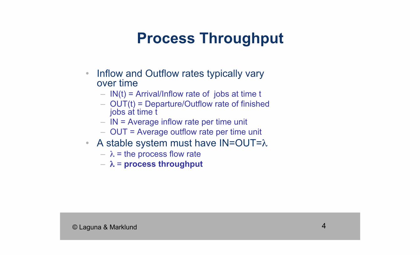
•  Inflow and Outflow rates typically vary over time –  IN(t) = Arrival/Inflow rate of jobs at time t –  OUT(t) = Departure/Outflow rate of finished

jobs at time t –  IN = Average inflow rate per time unit –  OUT = Average outflow rate per time unit

•  A stable system must have IN=OUT=λ –  λ = the process flow rate –  λ = process throughput

Process Throughput

© Laguna & Marklund

5

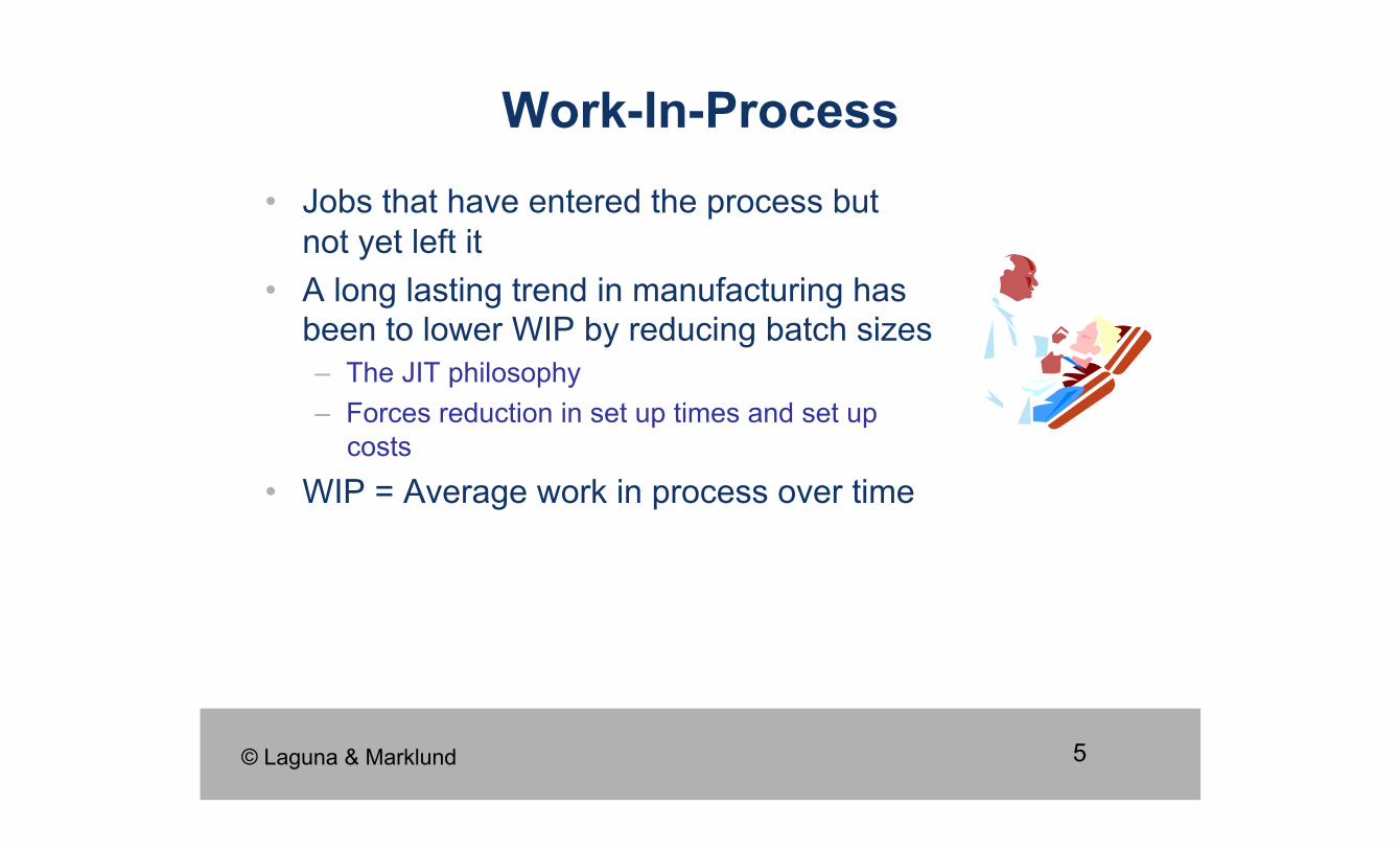
•  Jobs that have entered the process but not yet left it

•  A long lasting trend in manufacturing has been to lower WIP by reducing batch sizes –  The JIT philosophy –  Forces reduction in set up times and set up

costs

•  WIP = Average work in process over time

Work-In-Process


6

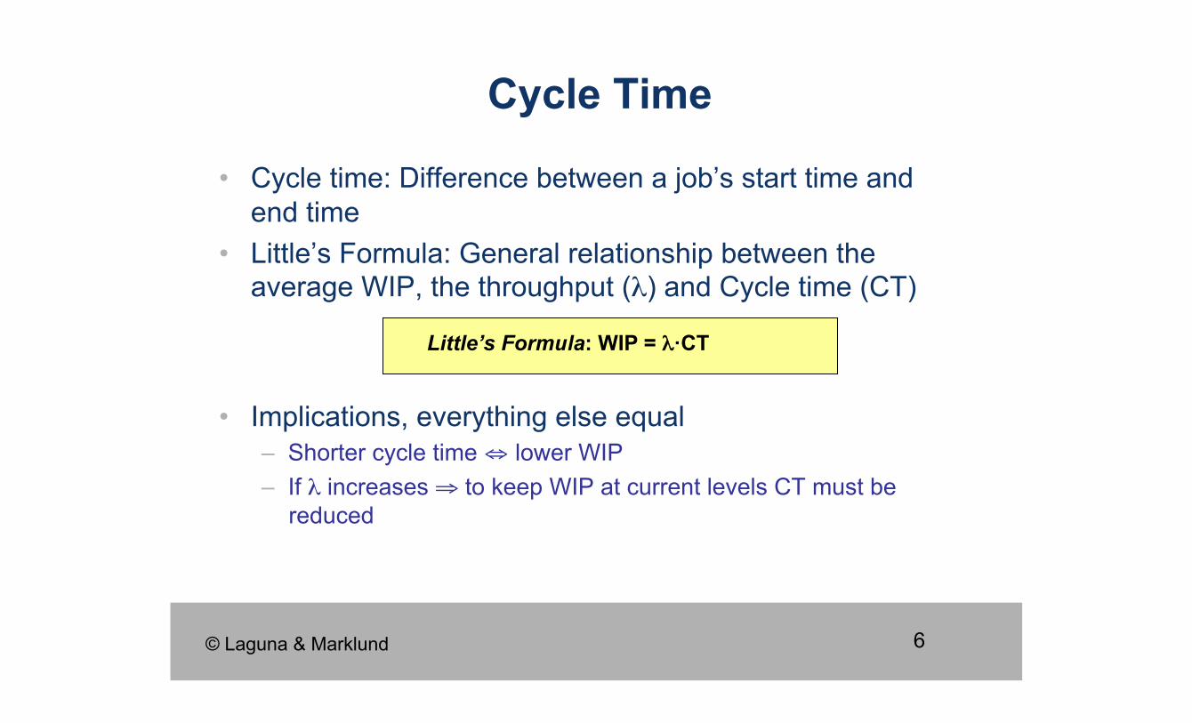
•  Cycle time: Difference between a job’s start time and end time

•  Little’s Formula: General relationship between the average WIP, the throughput (λ) and Cycle time (CT)

•  Implications, everything else equal –  Shorter cycle time ⇔ lower WIP –  If λ increases ⇒ to keep WIP at current levels CT must be

reduced

Cycle Time


Little’s Formula: WIP = λ·CT

7

Exercise 1

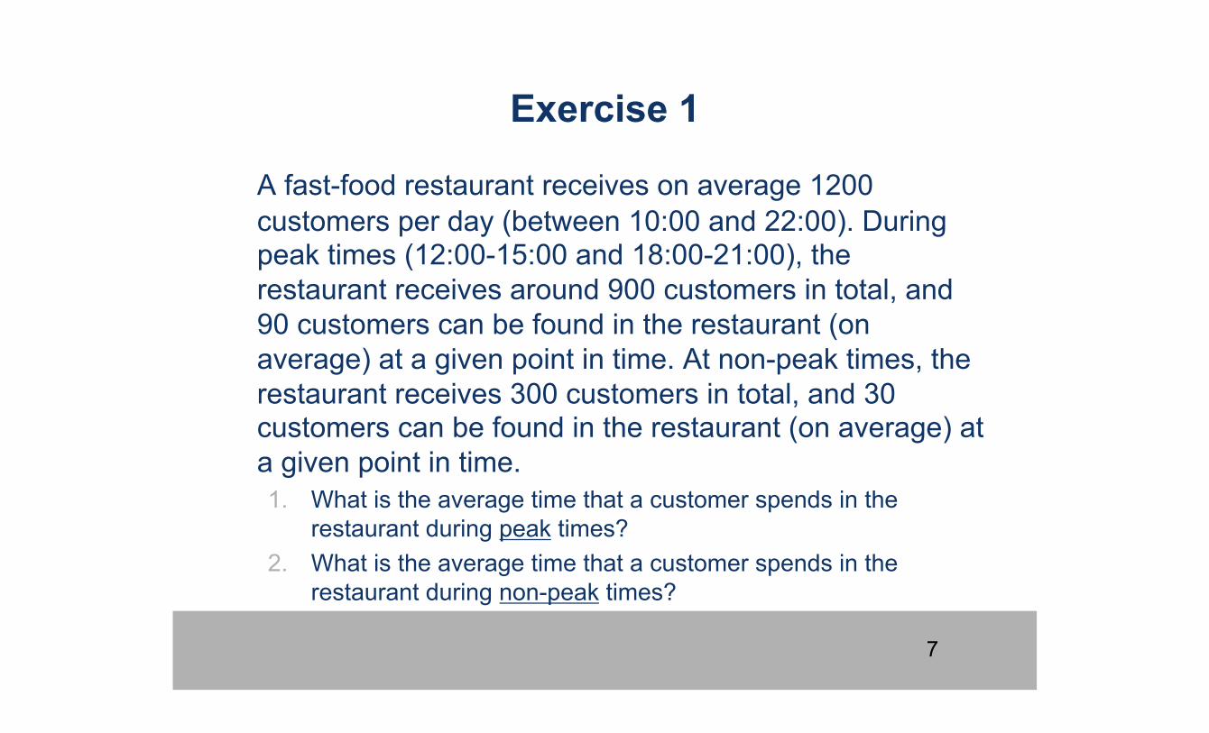
A fast-food restaurant receives on average 1200 customers per day (between 10:00 and 22:00). During peak times (12:00-15:00 and 18:00-21:00), the restaurant receives around 900 customers in total, and 90 customers can be found in the restaurant (on average) at a given point in time. At non-peak times, the restaurant receives 300 customers in total, and 30 customers can be found in the restaurant (on average) at a given point in time. 1.  What is the average time that a customer spends in the

restaurant during peak times? 2.  What is the average time that a customer spends in the

restaurant during non-peak times?

8

Exercise 1 (continued)

3.  The restaurant plans to launch a marketing campaign to attract more customers. However, the restaurant’s capacity is limited and becomes too full during peak times. What can the restaurant do to address this issue without investing in extending its building?

9

Cycle Time Analysis

•  Cycle time analysis: the task of calculating the average cycle time for an entire process or process segment –  Assumes that the average activity times for all involved activities

are available (activity time = waiting time + processing time)

•  In the simplest case a process consists of a sequence of activities on a single path –  The average cycle time is the sum of the average activity times

•  … but in general we must be able to account for –  Rework –  Multiple paths –  Parallel activities

10

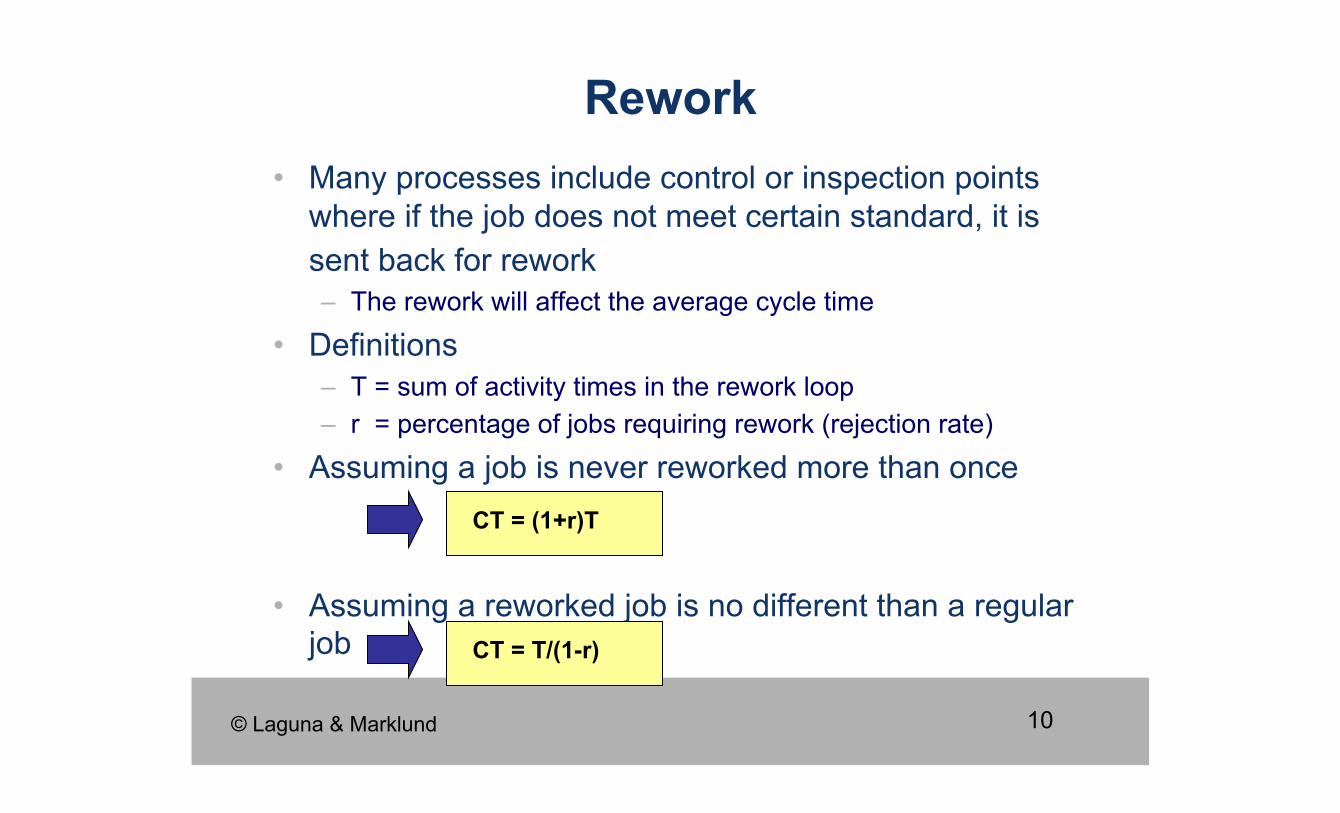
•  Many processes include control or inspection points where if the job does not meet certain standard, it is sent back for rework –  The rework will affect the average cycle time

•  Definitions –  T = sum of activity times in the rework loop –  r = percentage of jobs requiring rework (rejection rate)

•  Assuming a job is never reworked more than once

•  Assuming a reworked job is no different than a regular job

Rework

CT = (1+r)T

CT = T/(1-r)


11

Example – Rework effects on the average cycle time

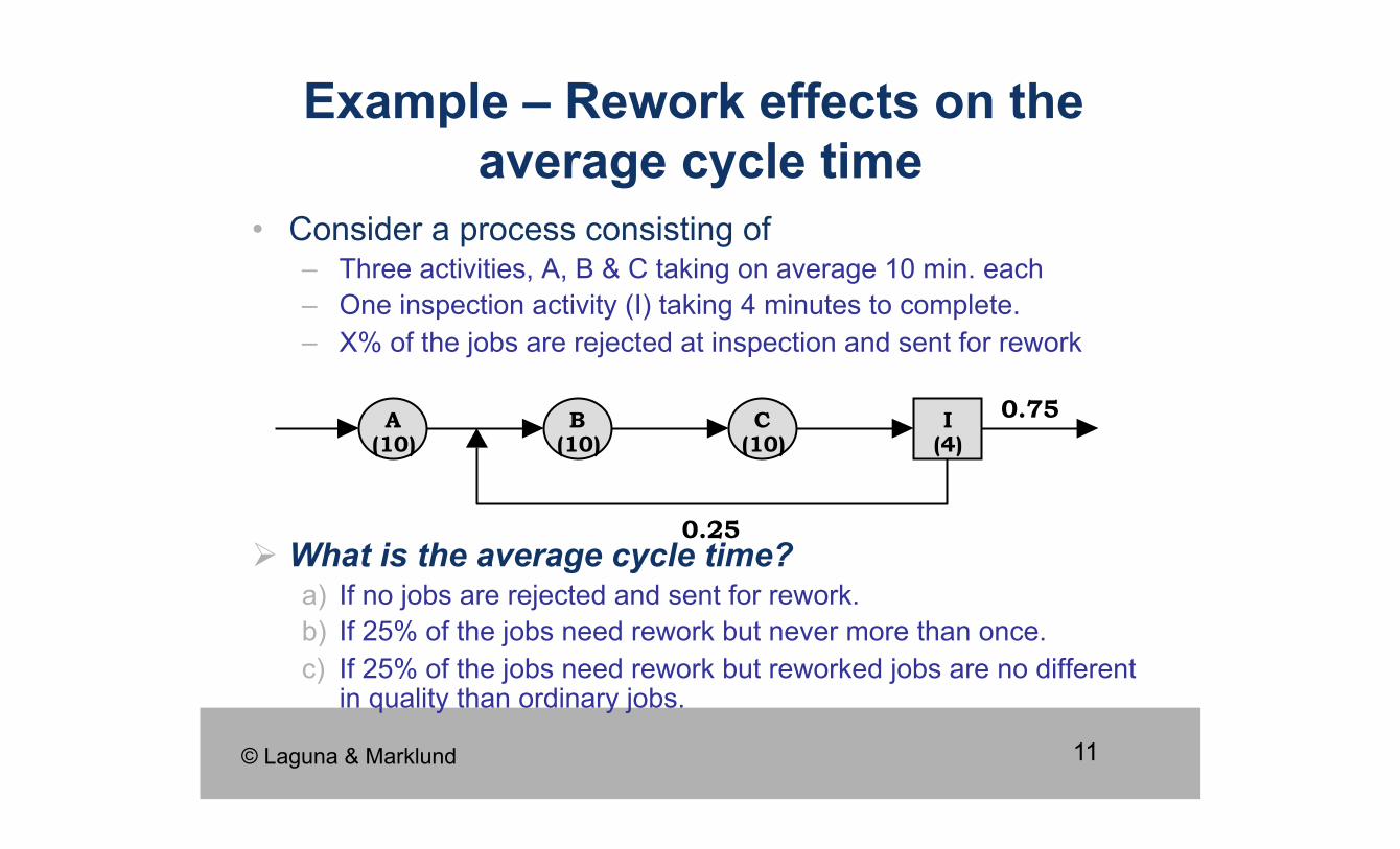
•  Consider a process consisting of –  Three activities, A, B & C taking on average 10 min. each –  One inspection activity (I) taking 4 minutes to complete. –  X% of the jobs are rejected at inspection and sent for rework

 What is the average cycle time? a)  If no jobs are rejected and sent for rework. b)  If 25% of the jobs need rework but never more than once. c)  If 25% of the jobs need rework but reworked jobs are no different

in quality than ordinary jobs.

0.75

0.25

A (10)

B (10)

C (10)

I (4)


12

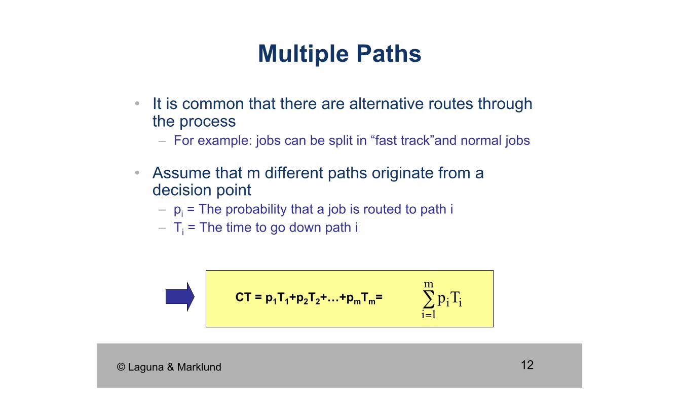
•  It is common that there are alternative routes through the process –  For example: jobs can be split in “fast track”and normal jobs

•  Assume that m different paths originate from a decision point –  pi = The probability that a job is routed to path i –  Ti = The time to go down path i

Multiple Paths

CT = p1T1+p2T2+…+pmTm=


13

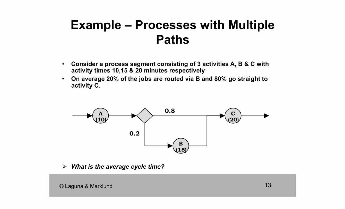
Example – Processes with Multiple Paths

•  Consider a process segment consisting of 3 activities A, B & C with activity times 10,15 & 20 minutes respectively

•  On average 20% of the jobs are routed via B and 80% go straight to activity C.

  What is the average cycle time?

0.8

0.2

A (10)

B (15)

C (20)


14

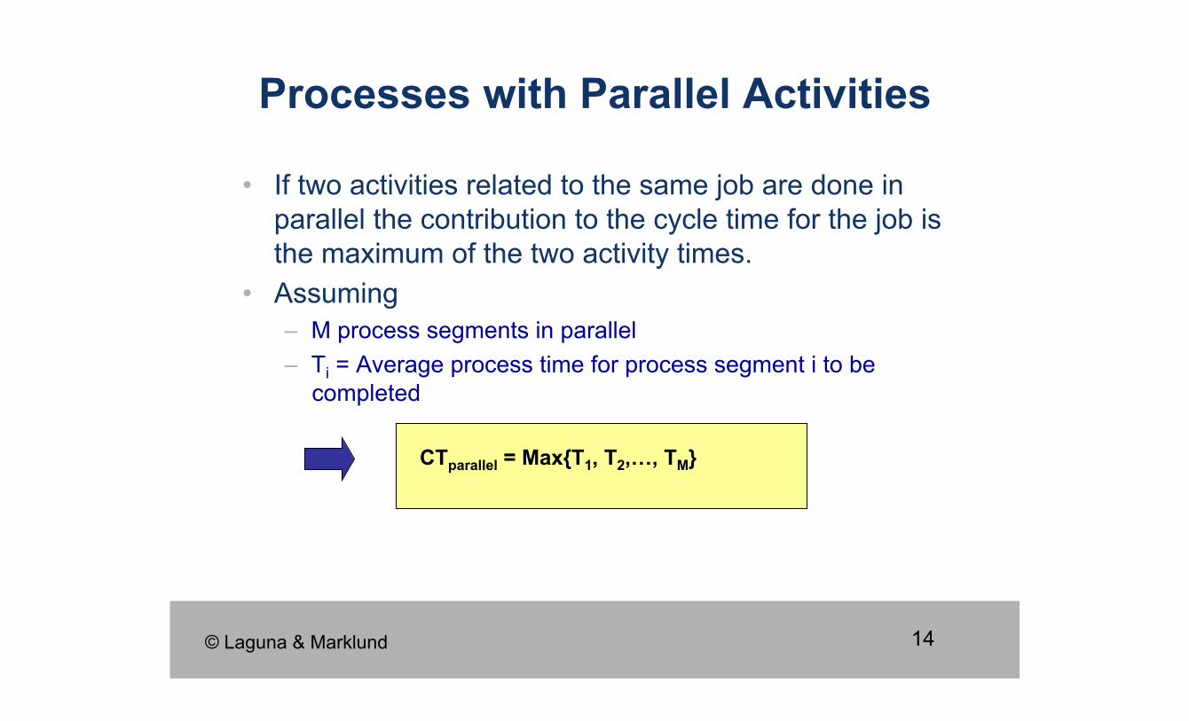
•  If two activities related to the same job are done in parallel the contribution to the cycle time for the job is the maximum of the two activity times.

•  Assuming –  M process segments in parallel –  Ti = Average process time for process segment i to be

completed

Processes with Parallel Activities

CTparallel = Max{T1, T2,…, TM}


15

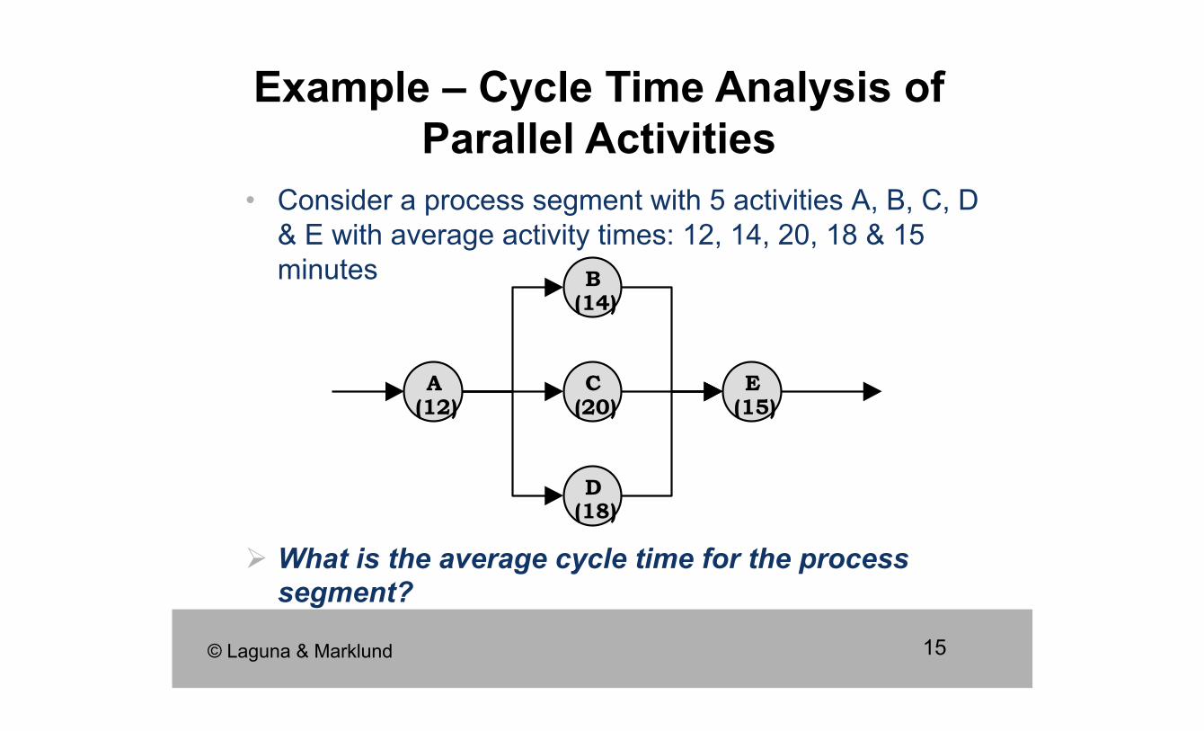
•  Consider a process segment with 5 activities A, B, C, D & E with average activity times: 12, 14, 20, 18 & 15 minutes

 What is the average cycle time for the process segment?

Example – Cycle Time Analysis of Parallel Activities

A (12)

B (14)

C (20)

D (18)

E (15)


16

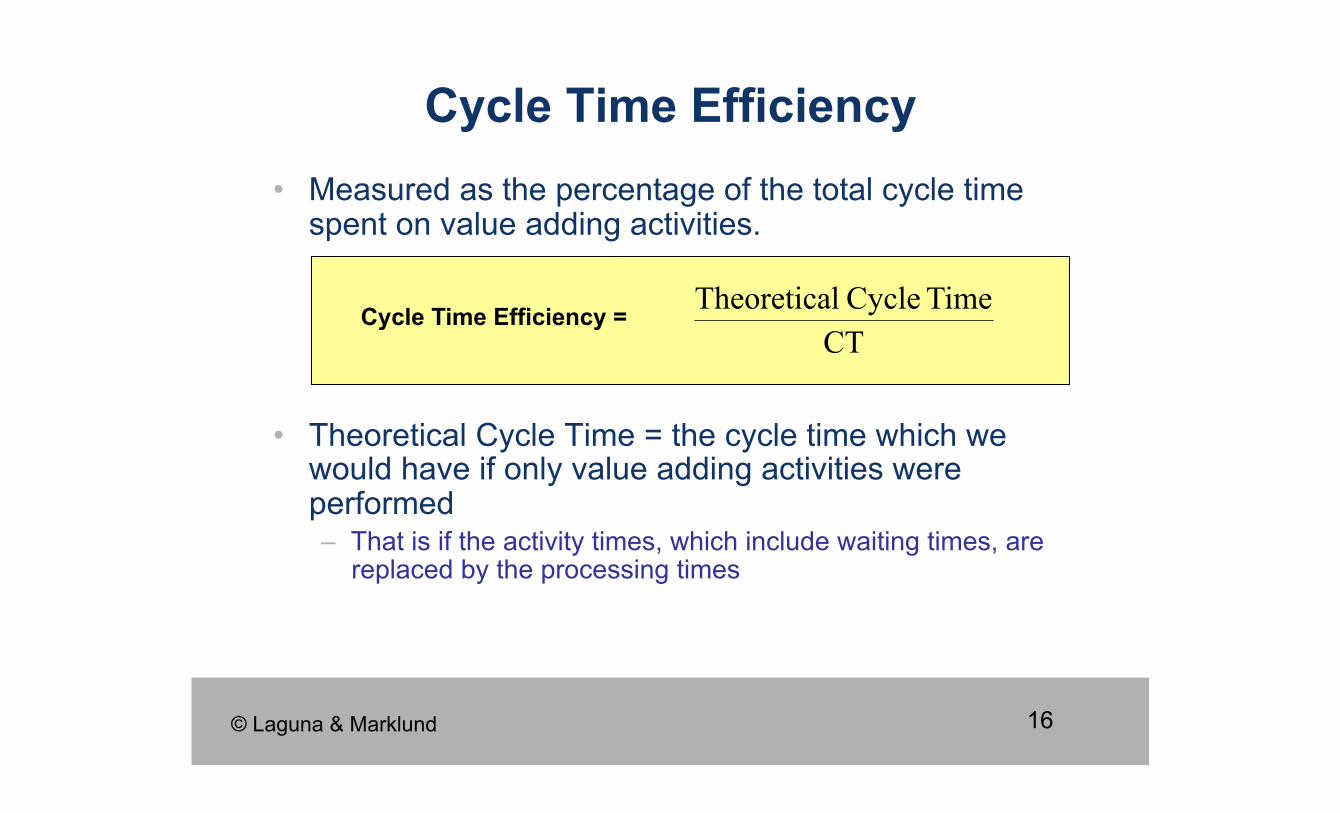
•  Measured as the percentage of the total cycle time spent on value adding activities.

•  Theoretical Cycle Time = the cycle time which we would have if only value adding activities were performed –  That is if the activity times, which include waiting times, are

replaced by the processing times

Cycle Time Efficiency

Cycle Time Efficiency =


17

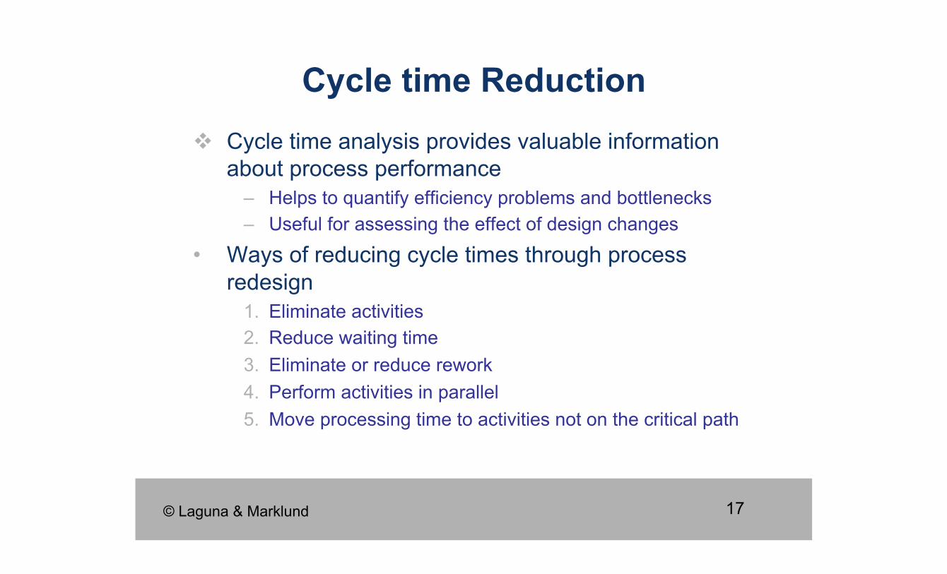
  Cycle time analysis provides valuable information about process performance

–  Helps to quantify efficiency problems and bottlenecks –  Useful for assessing the effect of design changes

•  Ways of reducing cycle times through process redesign

1.  Eliminate activities 2.  Reduce waiting time 3.  Eliminate or reduce rework 4.  Perform activities in parallel 5.  Move processing time to activities not on the critical path

Cycle time Reduction


18

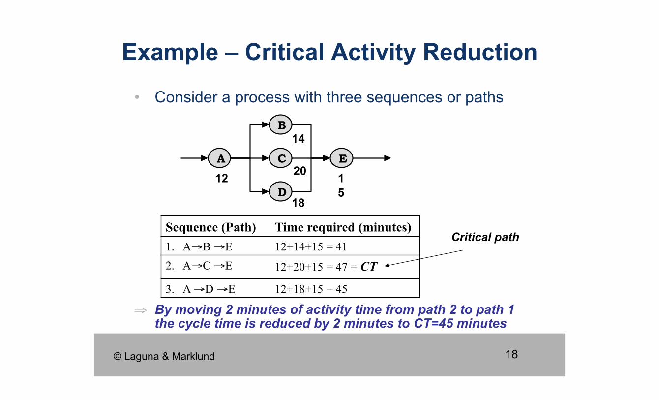
•  Consider a process with three sequences or paths

⇒  By moving 2 minutes of activity time from path 2 to path 1 the cycle time is reduced by 2 minutes to CT=45 minutes

Example – Critical Activity Reduction

A

B

C

D

E

12 15

18

20

14

Sequence (Path) Time required (minutes) 1. A→B →E 12+14+15 = 41 2. A→C →E 12+20+15 = 47 = CT

3. A →D →E 12+18+15 = 45

Critical path


19

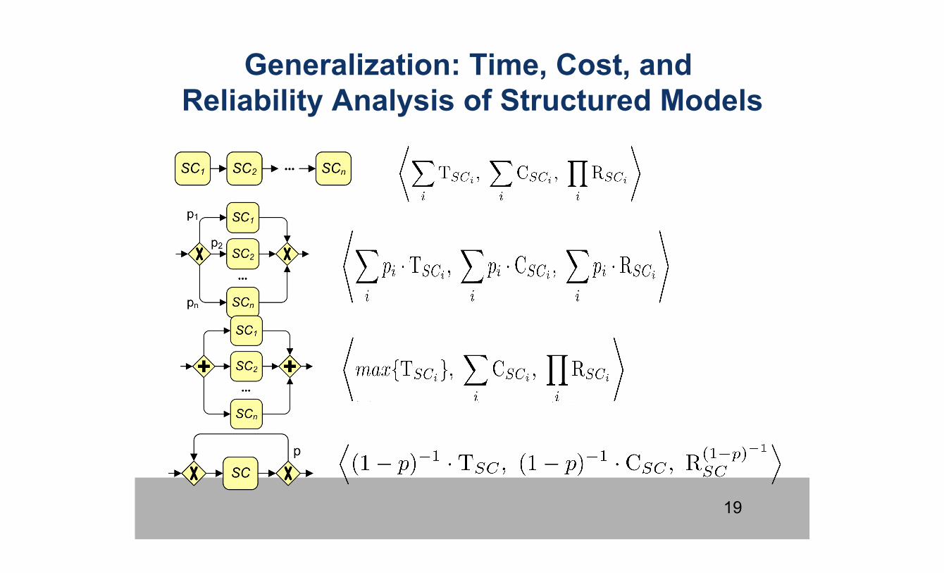
Generalization: Time, Cost, and Reliability Analysis of Structured Models

20

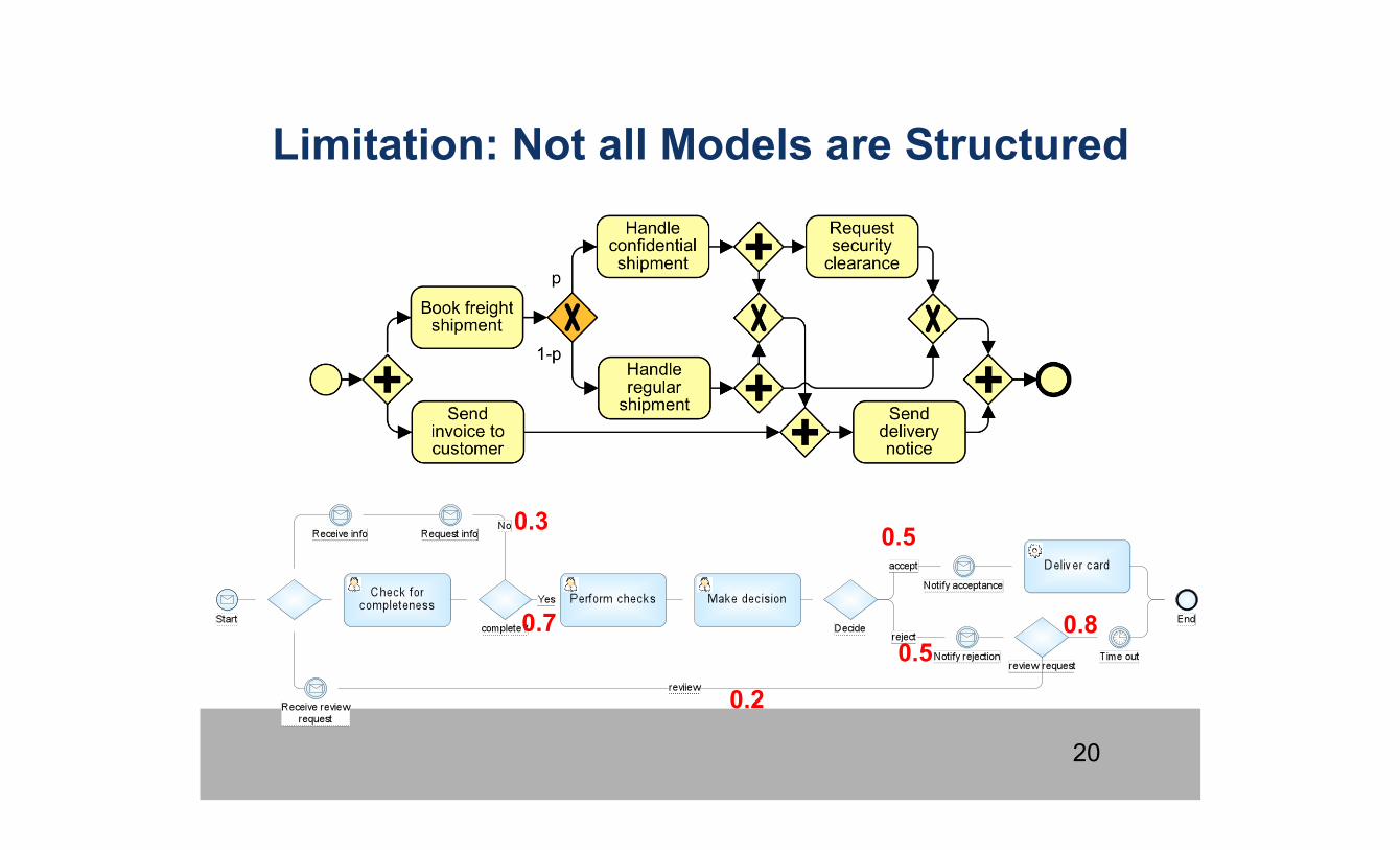
Limitation: Not all Models are Structured

0.5

0.7

0.3

0.5

0.2

0.8

21

•  Focus on assessing the capacity needs and resource utilization in the process

1.  Determine the number of jobs flowing through different tasks (flow rate)

2.  Determine capacity requirements and utilization based on the flow rates obtained in 1.

3.  Determine bottlenecks

•  Complements cycle time analysis…

Capacity Analysis


22

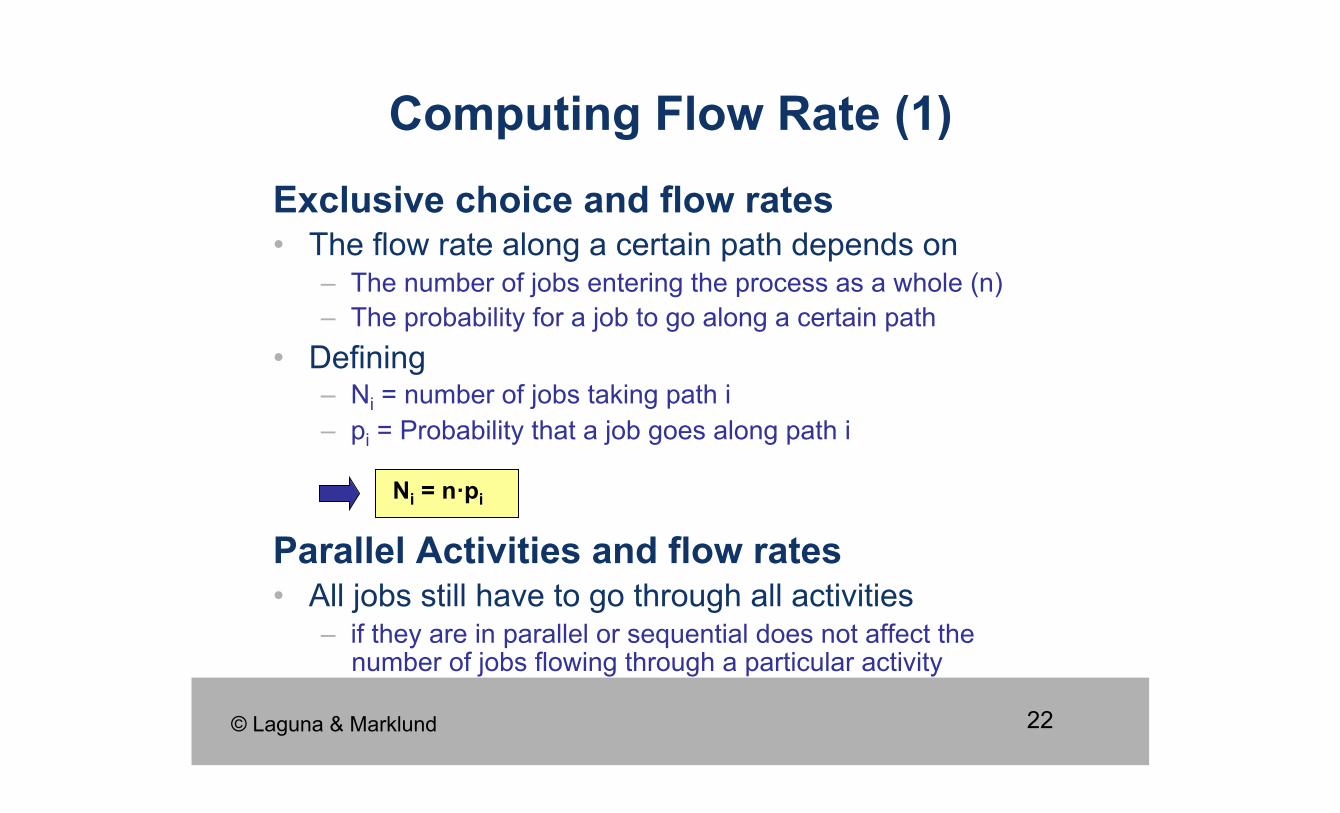
Exclusive choice and flow rates •  The flow rate along a certain path depends on

–  The number of jobs entering the process as a whole (n) –  The probability for a job to go along a certain path

•  Defining –  Ni = number of jobs taking path i –  pi = Probability that a job goes along path i

Parallel Activities and flow rates •  All jobs still have to go through all activities

–  if they are in parallel or sequential does not affect the number of jobs flowing through a particular activity

Computing Flow Rate (1)

Ni = n·pi


23

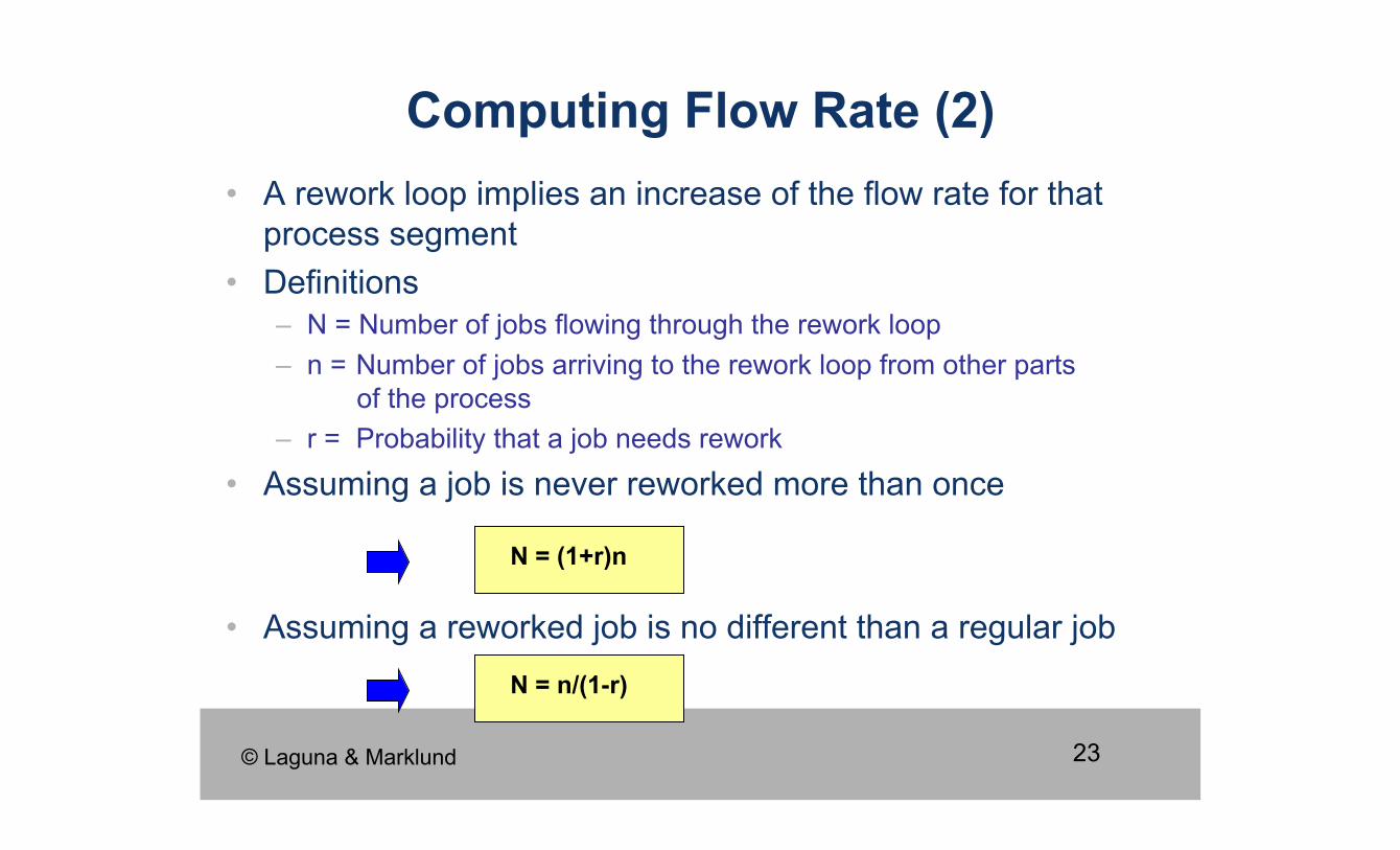
•  A rework loop implies an increase of the flow rate for that process segment

•  Definitions –  N = Number of jobs flowing through the rework loop –  n = Number of jobs arriving to the rework loop from other parts

of the process –  r = Probability that a job needs rework

•  Assuming a job is never reworked more than once

•  Assuming a reworked job is no different than a regular job

Computing Flow Rate (2)

N = (1+r)n

N = n/(1-r)


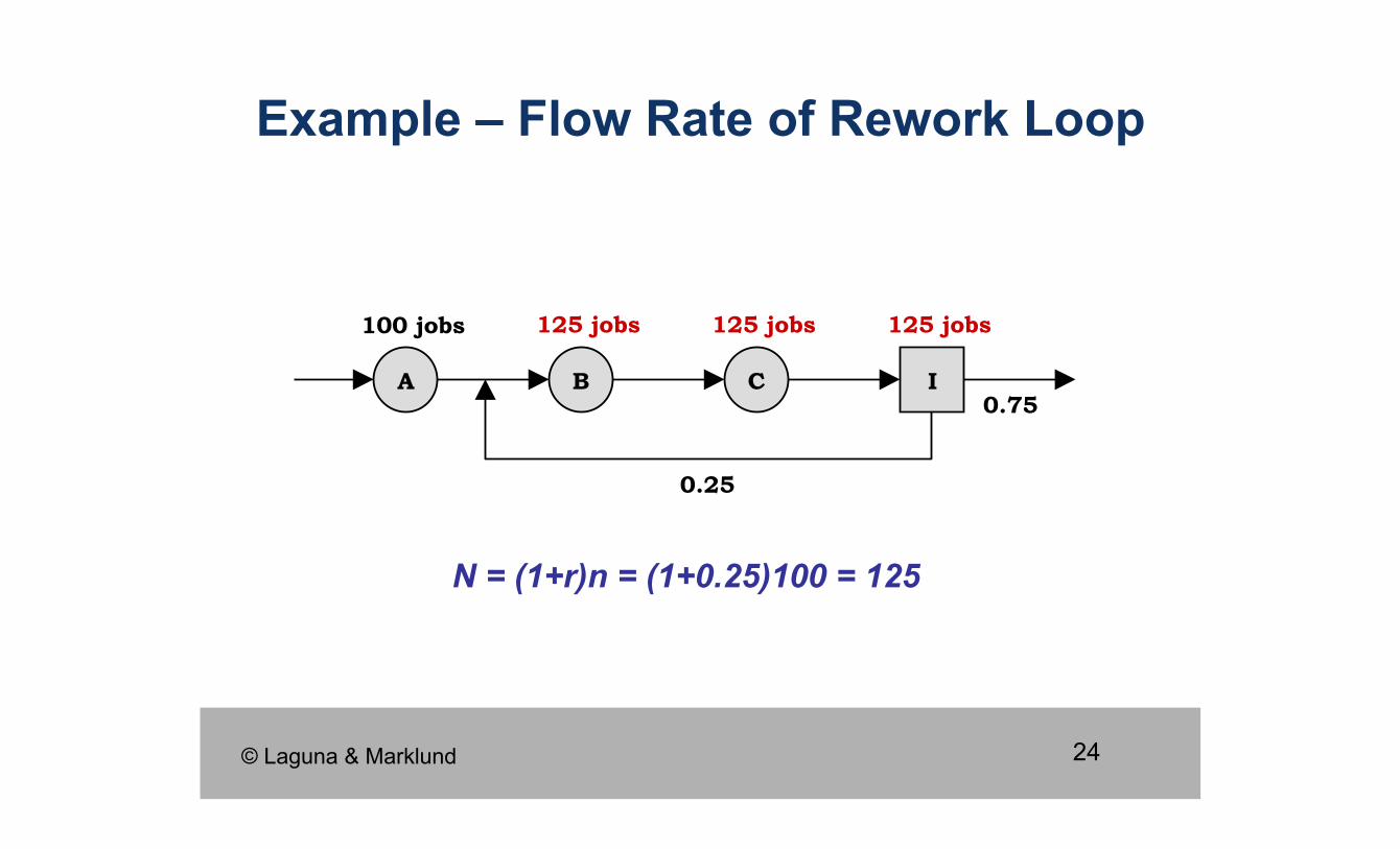
24

N = (1+r)n = (1+0.25)100 = 125

Example – Flow Rate of Rework Loop

0.75

0.25

A B C I

100 jobs 125 jobs 125 jobs 125 jobs


25

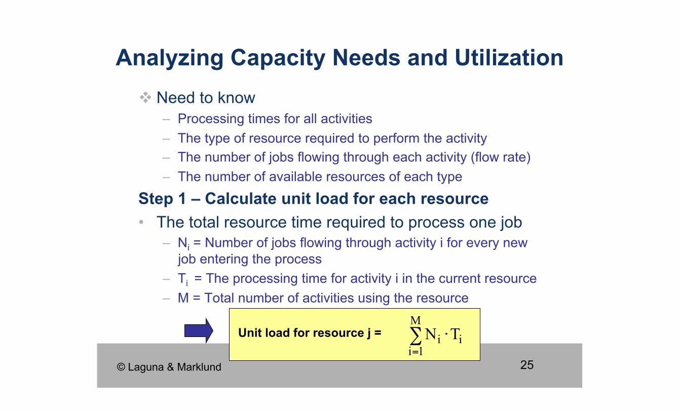
 Need to know –  Processing times for all activities –  The type of resource required to perform the activity –  The number of jobs flowing through each activity (flow rate) –  The number of available resources of each type

Step 1 – Calculate unit load for each resource •  The total resource time required to process one job

–  Ni = Number of jobs flowing through activity i for every new job entering the process

–  Ti = The processing time for activity i in the current resource –  M = Total number of activities using the resource

Analyzing Capacity Needs and Utilization

Unit load for resource j =


26

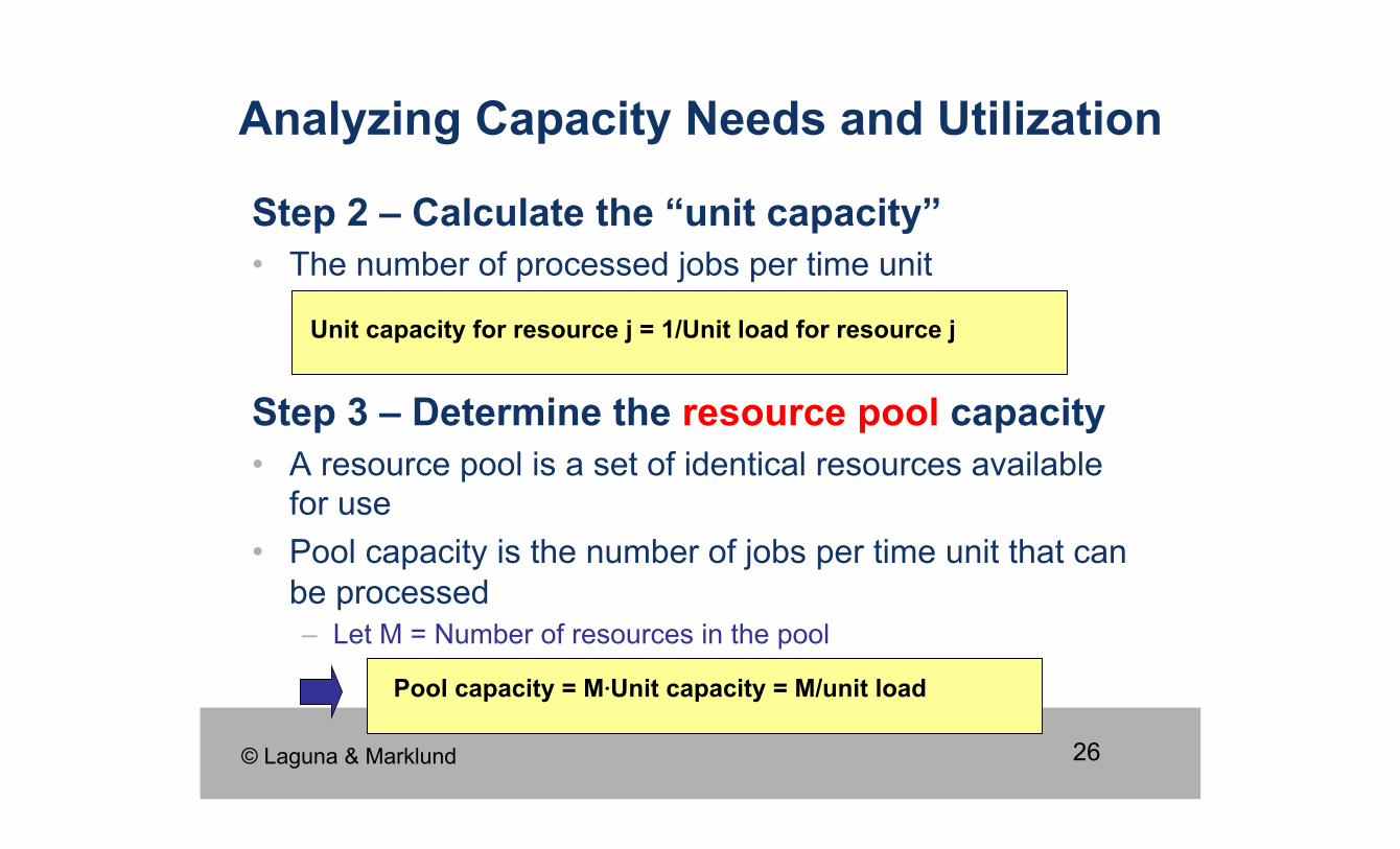
Step 2 – Calculate the “unit capacity” •  The number of processed jobs per time unit

Step 3 – Determine the resource pool capacity •  A resource pool is a set of identical resources available

for use •  Pool capacity is the number of jobs per time unit that can

be processed –  Let M = Number of resources in the pool

Analyzing Capacity Needs and Utilization

Unit capacity for resource j = 1/Unit load for resource j

Pool capacity = M⋅Unit capacity = M/unit load


27

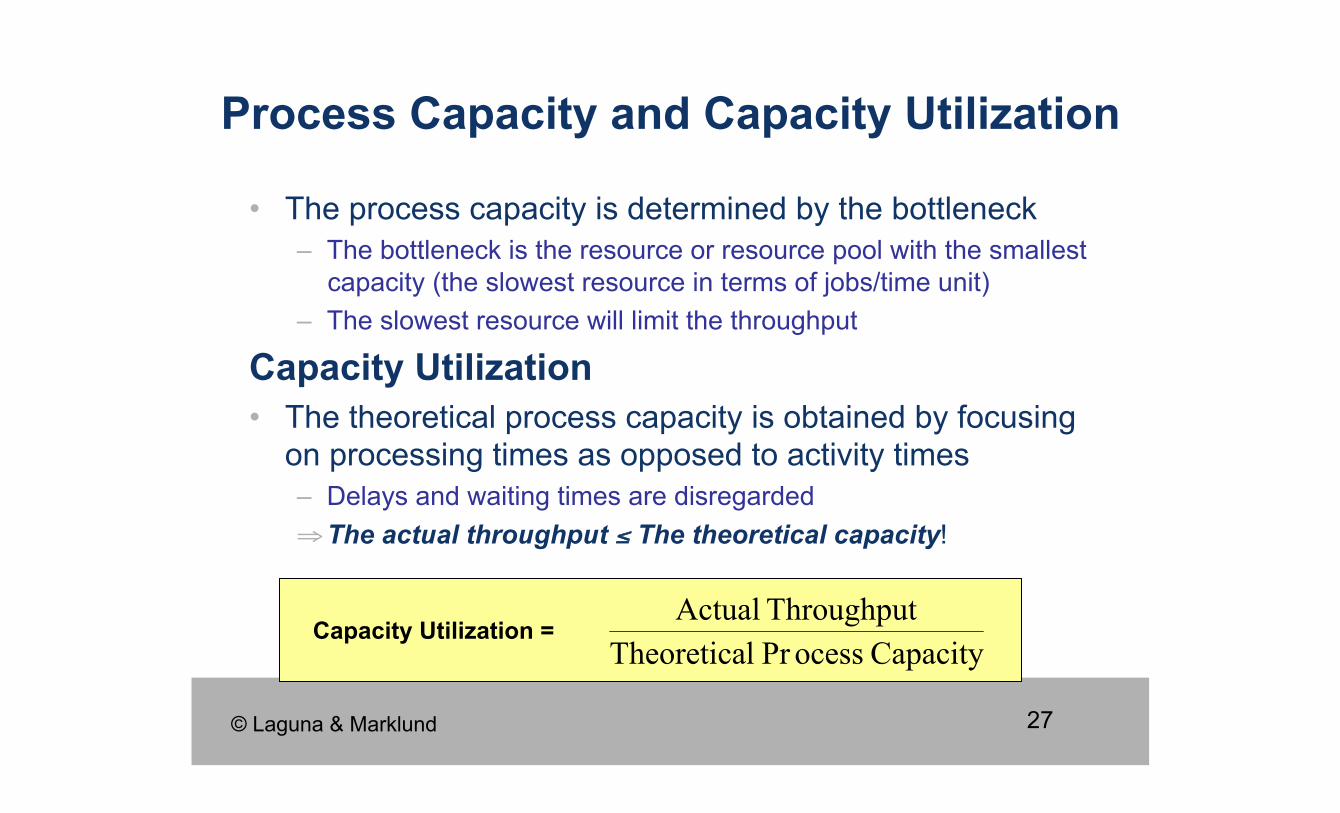
•  The process capacity is determined by the bottleneck –  The bottleneck is the resource or resource pool with the smallest

capacity (the slowest resource in terms of jobs/time unit) –  The slowest resource will limit the throughput

Capacity Utilization •  The theoretical process capacity is obtained by focusing

on processing times as opposed to activity times –  Delays and waiting times are disregarded ⇒ The actual throughput ≤ The theoretical capacity!

Process Capacity and Capacity Utilization

Capacity Utilization =


28

Limitations of Cycle Time/Capacity Analysis

•  Cycle time analysis and capacity do not consider waiting times due to resource contention

•  Queuing analysis and simulation address these limitations and have a broader applicability

29

 State of the system = number of customers in the system  Queue length = (state of the system) – (number of

customers being served)

λ = Average arrival intensity (= # arrivals per time unit)

µ = Average service intensity for the system

ρ = Utilization factor = The expected fraction of time that the service facility is being used

Queuing Theory: Notation


30

•  Capacity problems are very common in industry and one of the main drivers of process redesign –  Need to balance the cost of increased capacity against the

gains of increased productivity and service •  Queuing and waiting time analysis is particularly

important in service systems –  Large costs of waiting and of lost sales due to waiting

Prototype Example – ER at a Hospital •  Patients arrive by ambulance or by their own accord •  One doctor is always on duty •  More patients seeks help ⇒ longer waiting times  Question: Should another MD position be

instated?

Why is Queuing Analysis Important?


31

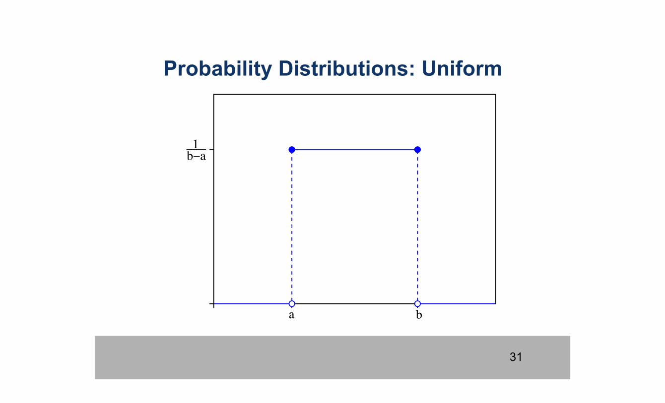
Probability Distributions: Uniform

32

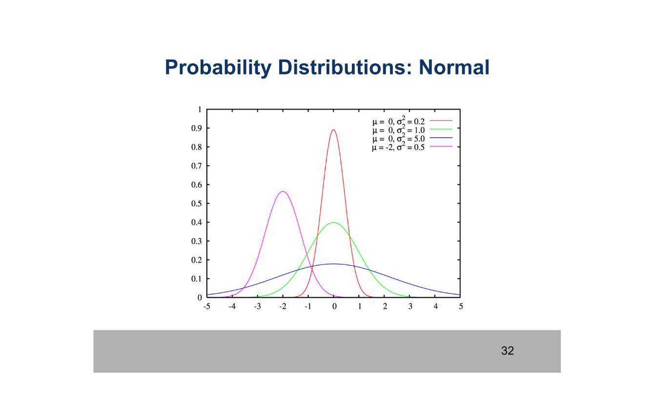
Probability Distributions: Normal

33

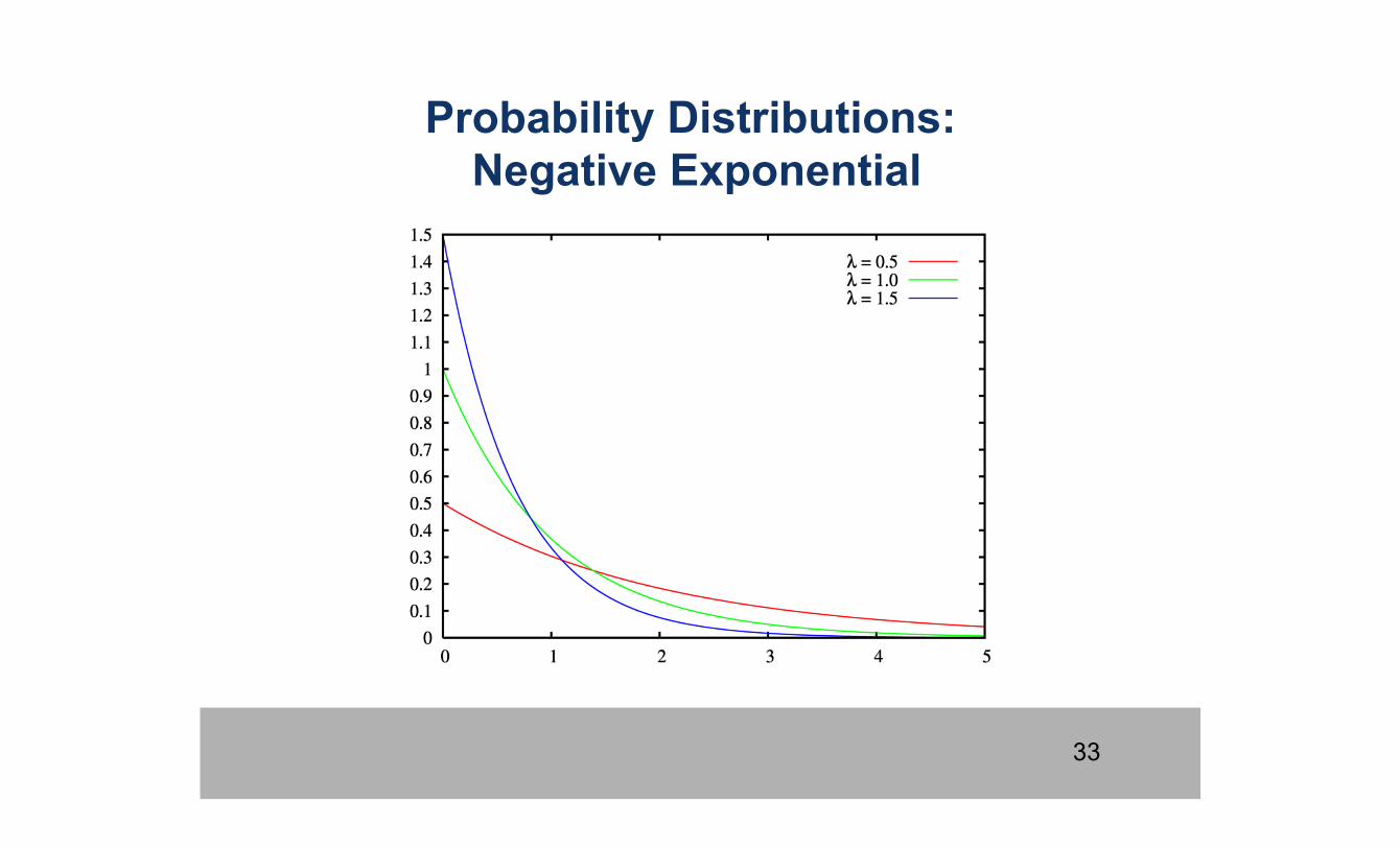
Probability Distributions: Negative Exponential

34

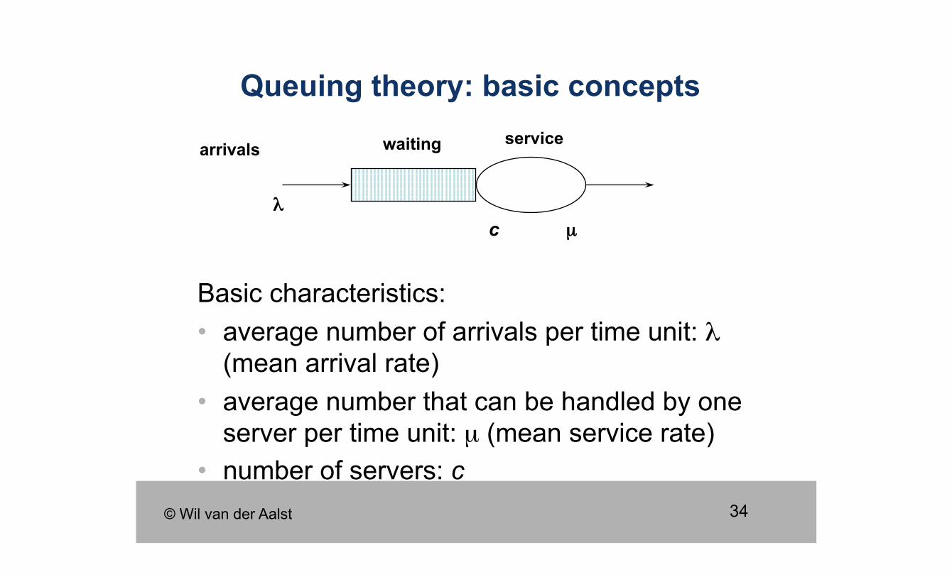
Queuing theory: basic concepts

Basic characteristics: •  average number of arrivals per time unit: λ

(mean arrival rate) •  average number that can be handled by one

server per time unit: µ (mean service rate) •  number of servers: c

arrivals waiting service

λ µ c

© Wil van der Aalst

35

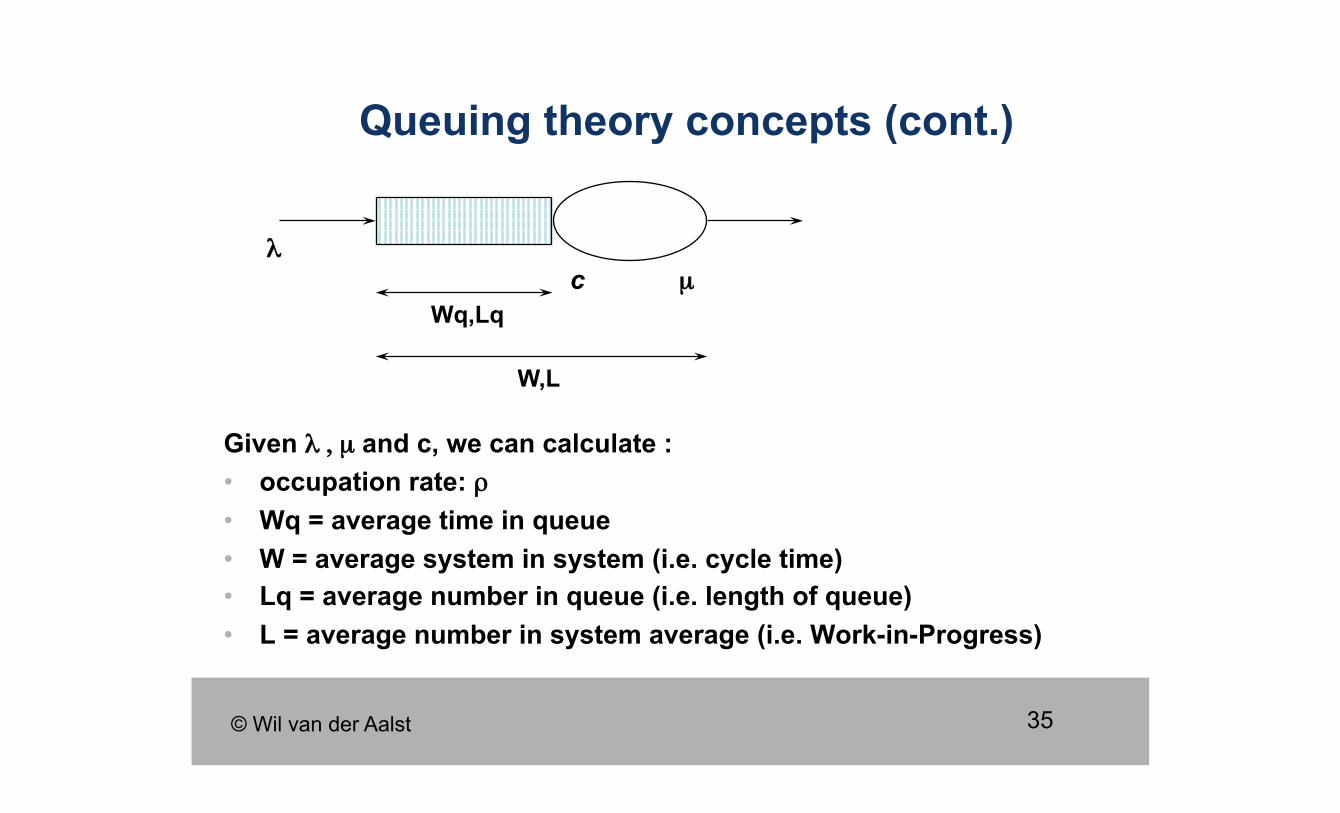
Queuing theory concepts (cont.)

Given λ , µ and c, we can calculate : •  occupation rate: ρ •  Wq = average time in queue •  W = average system in system (i.e. cycle time) •  Lq = average number in queue (i.e. length of queue) •  L = average number in system average (i.e. Work-in-Progress)

λ µ c

Wq,Lq

W,L

© Wil van der Aalst

36

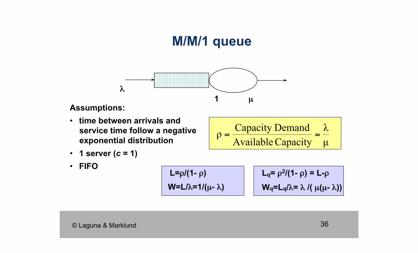
M/M/1 queue

λ µ 1

Assumptions: •  time between arrivals and

service time follow a negative exponential distribution

•  1 server (c = 1) •  FIFO

L=ρ/(1- ρ) Lq= ρ2/(1- ρ) = L-ρ W=L/λ=1/(µ- λ) Wq=Lq/λ= λ /( µ(µ- λ))


37

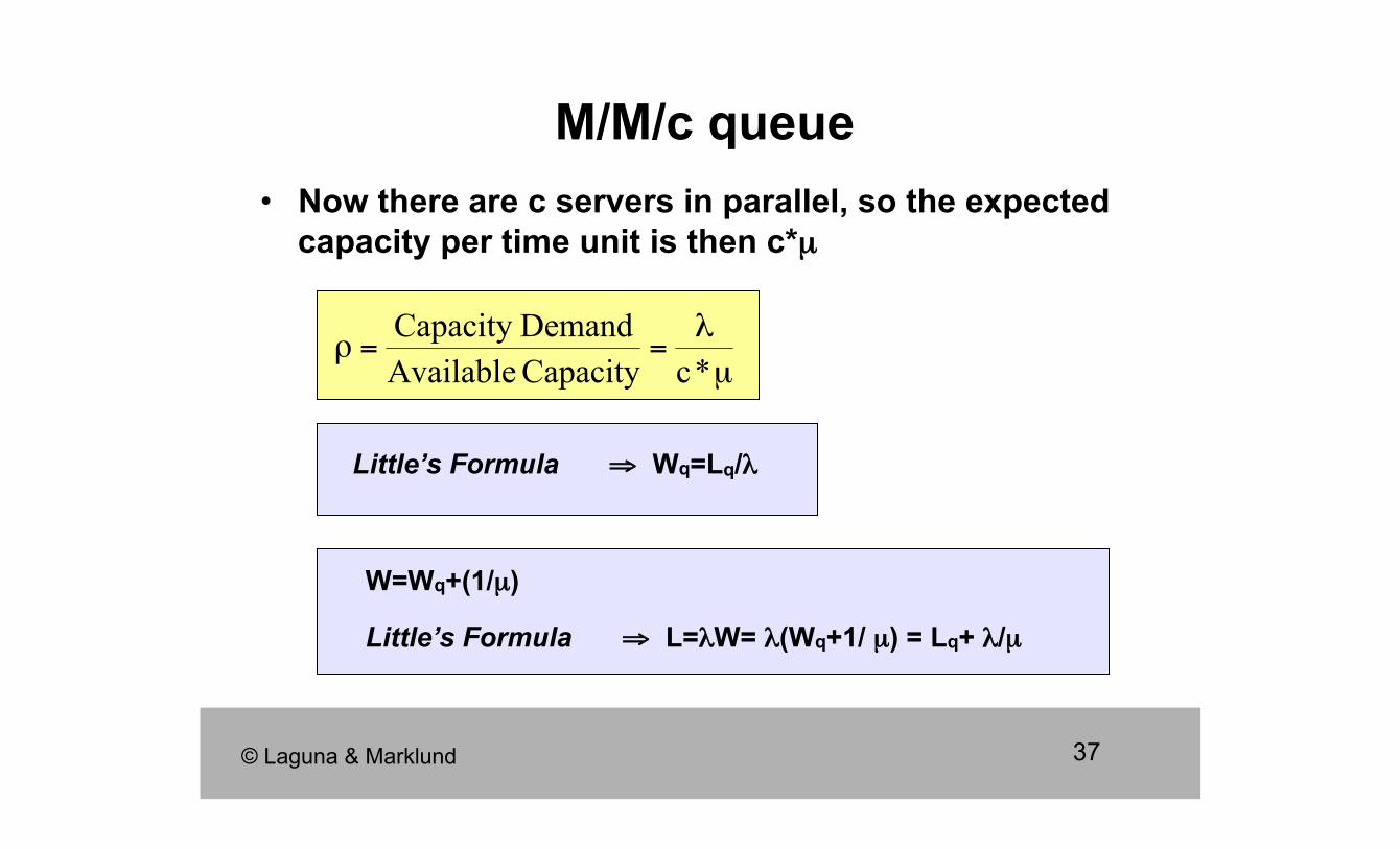
M/M/c queue •  Now there are c servers in parallel, so the expected

capacity per time unit is then c*µ

W=Wq+(1/µ)

Little’s Formula ⇒ Wq=Lq/λ

Little’s Formula ⇒ L=λW= λ(Wq+1/ µ) = Lq+ λ/µ


38

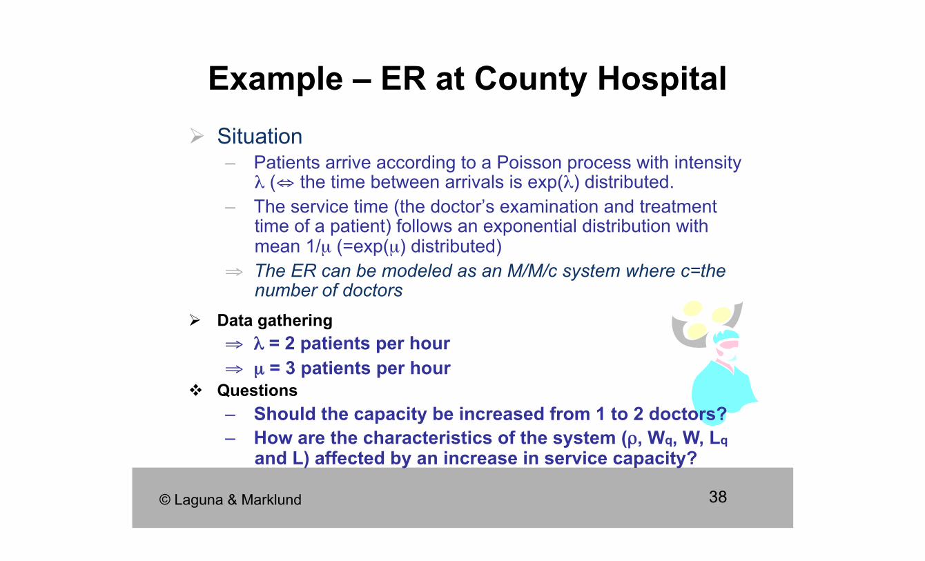
  Situation –  Patients arrive according to a Poisson process with intensity

λ (⇔ the time between arrivals is exp(λ) distributed. –  The service time (the doctor’s examination and treatment

time of a patient) follows an exponential distribution with mean 1/µ (=exp(µ) distributed)

⇒  The ER can be modeled as an M/M/c system where c=the number of doctors

Example – ER at County Hospital

  Data gathering ⇒  λ = 2 patients per hour ⇒  µ = 3 patients per hour

  Questions –  Should the capacity be increased from 1 to 2 doctors? –  How are the characteristics of the system (ρ, Wq, W, Lq

and L) affected by an increase in service capacity?


39

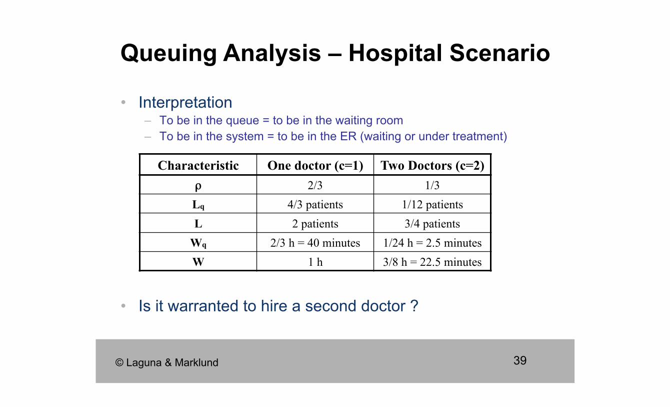
•  Interpretation –  To be in the queue = to be in the waiting room –  To be in the system = to be in the ER (waiting or under treatment)

•  Is it warranted to hire a second doctor ?

Queuing Analysis – Hospital Scenario

Characteristic One doctor (c=1) Two Doctors (c=2) ρ 2/3 1/3 Lq 4/3 patients 1/12 patients L 2 patients 3/4 patients

Wq 2/3 h = 40 minutes 1/24 h = 2.5 minutes W 1 h 3/8 h = 22.5 minutes


40

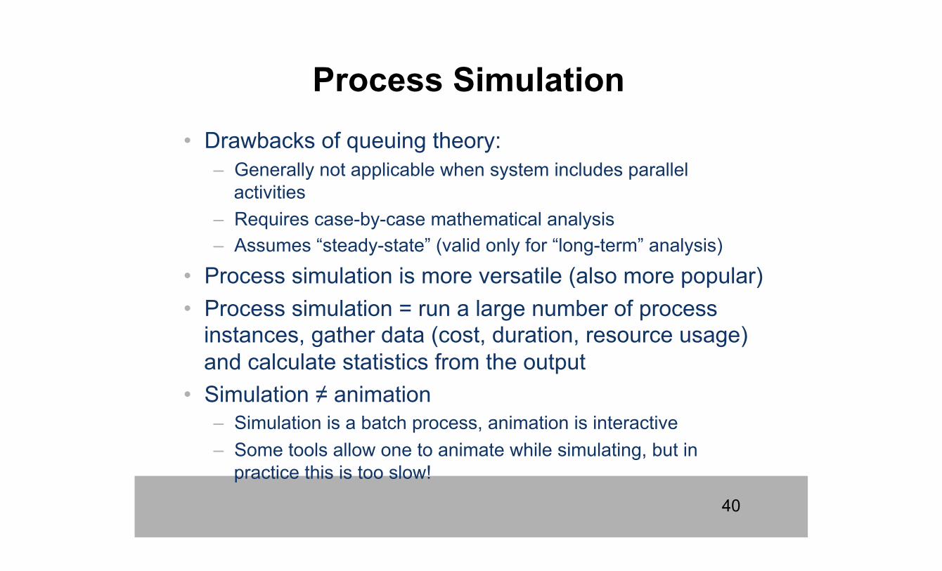
•  Drawbacks of queuing theory: –  Generally not applicable when system includes parallel

activities –  Requires case-by-case mathematical analysis –  Assumes “steady-state” (valid only for “long-term” analysis)

•  Process simulation is more versatile (also more popular) •  Process simulation = run a large number of process

instances, gather data (cost, duration, resource usage) and calculate statistics from the output

•  Simulation ≠ animation –  Simulation is a batch process, animation is interactive –  Some tools allow one to animate while simulating, but in

practice this is too slow!

Process Simulation

41

Process Simulation

•  Basic steps in evaluating a process model with simulation 1. Building the simulation model 2. Running the simulation 3. Analyzing the simulation results (performance

measure) 4. Evaluation of alternative scenarios

42

Elements of a simulation model

•  The process model including: –  Activities, control-flow relations (flows, gateways) –  Resources and resource pools (i.e. roles)

•  Resource requirements: mapping between activities and resource pools

•  Processing times (per activity, or per activity-resource pair)

•  Costs (per activity, or per activity-resource pair) •  Arrival rate (also called: token creation) •  Conditional branching probabilities (XOR gateways)

43

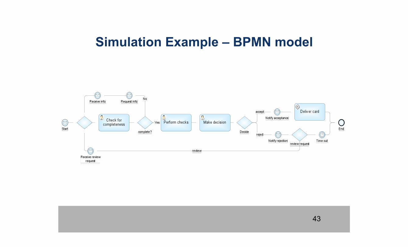
Simulation Example – BPMN model

44

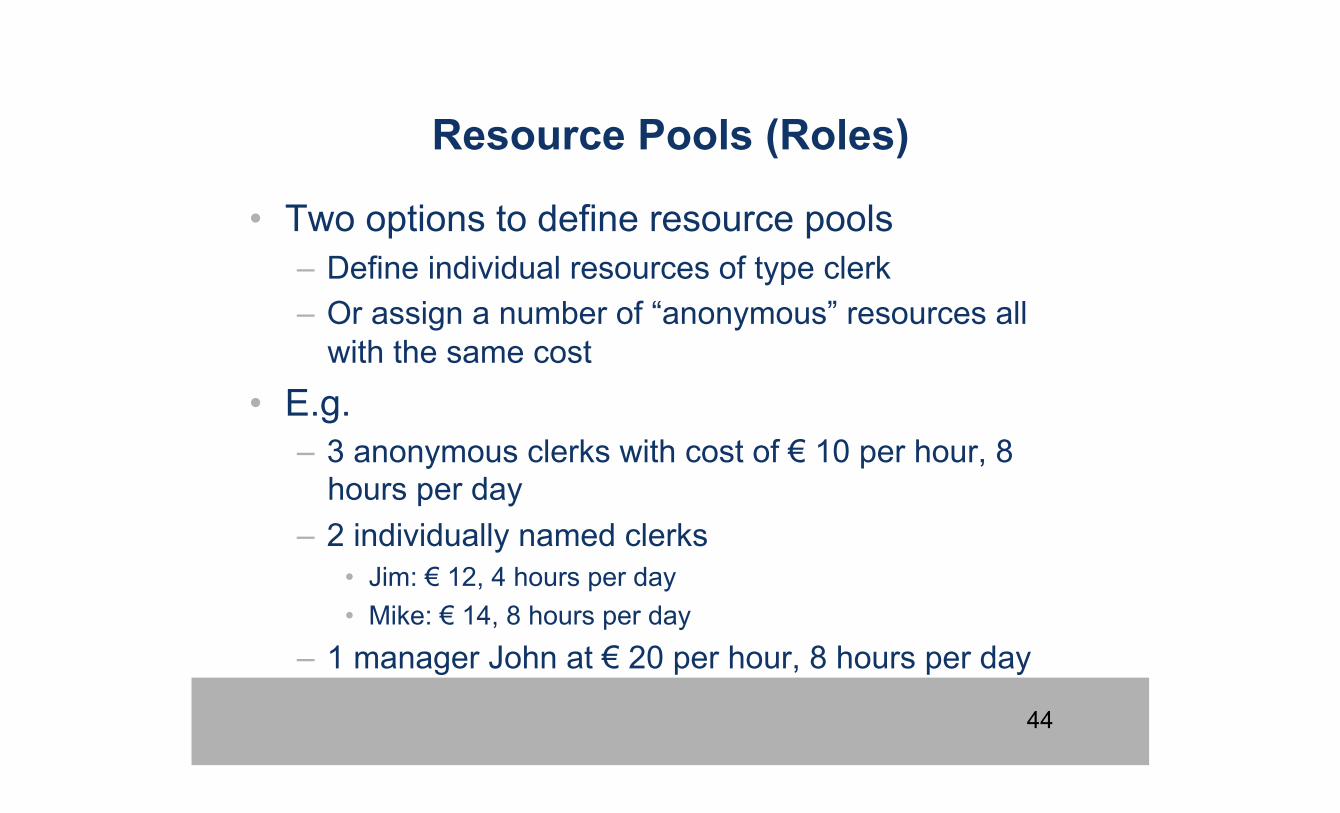
Resource Pools (Roles)

•  Two options to define resource pools –  Define individual resources of type clerk –  Or assign a number of “anonymous” resources all

with the same cost •  E.g.

–  3 anonymous clerks with cost of € 10 per hour, 8 hours per day

–  2 individually named clerks •  Jim: € 12, 4 hours per day •  Mike: € 14, 8 hours per day

–  1 manager John at € 20 per hour, 8 hours per day

45

Resource pools and execution times Task Role Execution Time

Normal distribution: mean and std deviation

Receive application system 0 0 Check completeness Clerk 30 mins 10 mins Perform checks Clerk 2 hours 1 hour Request info system 1 min 0 Receive info (Event) system 48 hours 24 hours Make decision Manager 1 hour 30 mins Notify rejection system 1 min 0 Time out (Time) system 72 hours 0 Receive review request (Event) system 48 hours 12 hours Notify acceptance system 1 min 0 Deliver Credit card system 1 hour 0

Alternative: assign execution times to the tasks only (like in cycle time analysis)

46

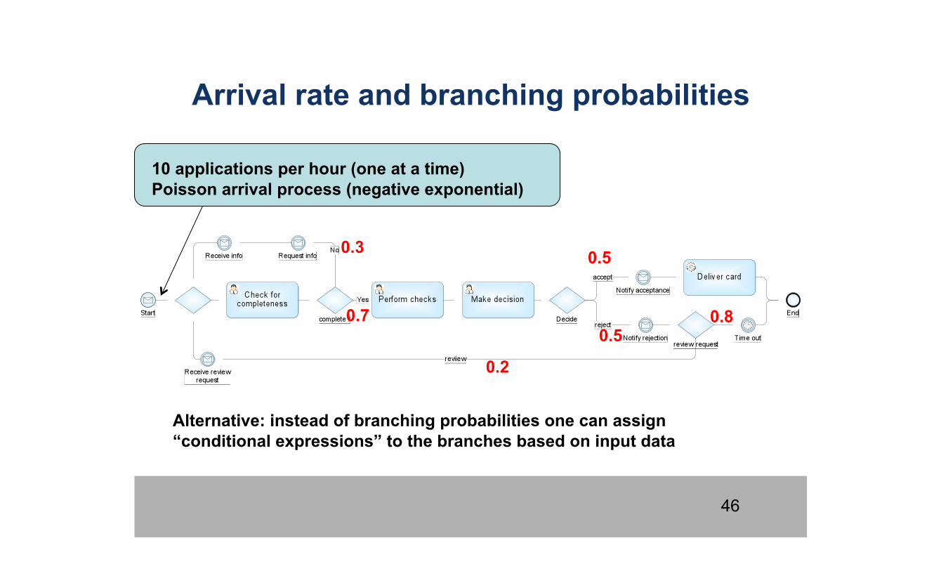
Arrival rate and branching probabilities

10 applications per hour (one at a time) Poisson arrival process (negative exponential)

0.5

0.7

0.3

0.5

Alternative: instead of branching probabilities one can assign “conditional expressions” to the branches based on input data

0.2

0.8

47

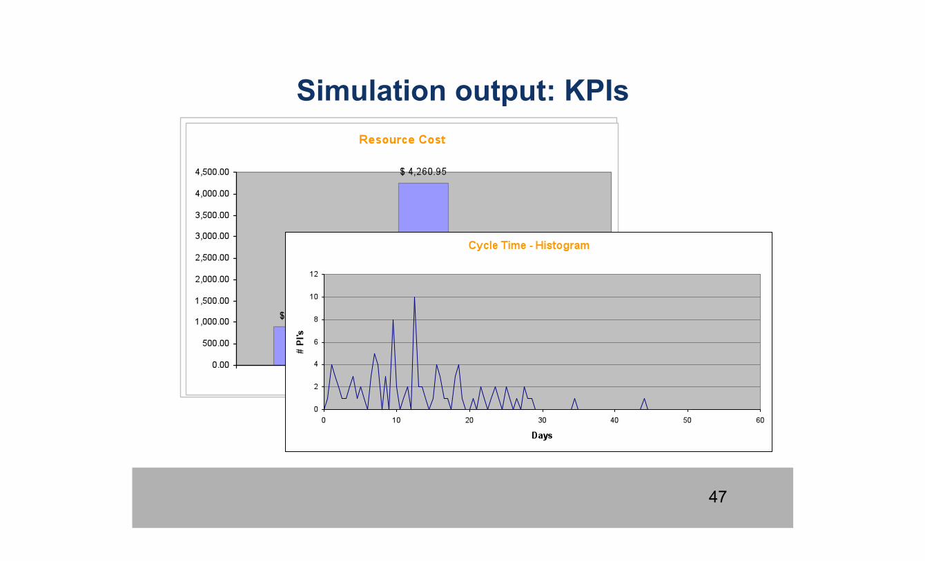
Simulation output: KPIs

48

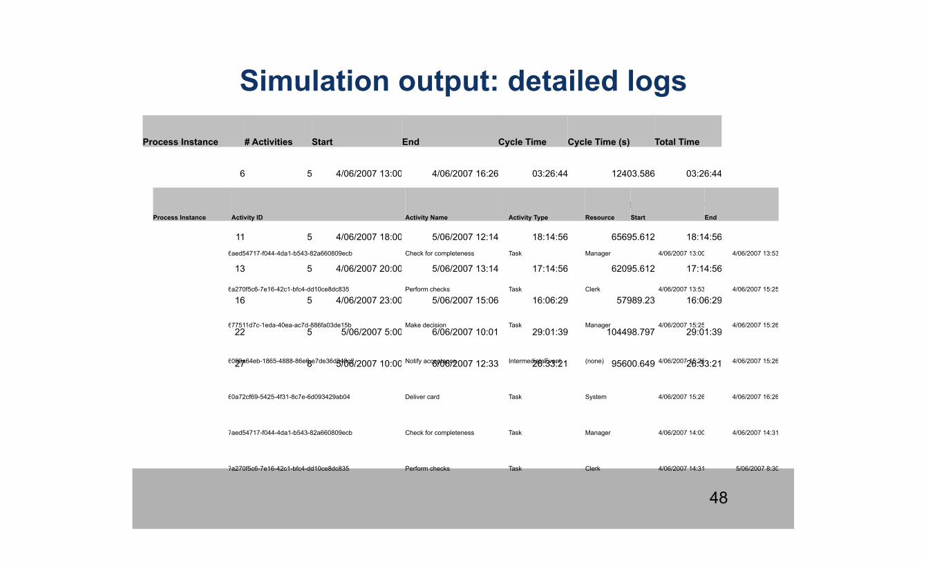
Simulation output: detailed logs

Process Instance # Activities Start End Cycle Time Cycle Time (s) Total Time

6 5 4/06/2007 13:00 4/06/2007 16:26 03:26:44 12403.586 03:26:44

7 5 4/06/2007 14:00 5/06/2007 9:30 19:30:38 70238.376 19:30:38

11 5 4/06/2007 18:00 5/06/2007 12:14 18:14:56 65695.612 18:14:56

13 5 4/06/2007 20:00 5/06/2007 13:14 17:14:56 62095.612 17:14:56

16 5 4/06/2007 23:00 5/06/2007 15:06 16:06:29 57989.23 16:06:29

22 5 5/06/2007 5:00 6/06/2007 10:01 29:01:39 104498.797 29:01:39

27 8 5/06/2007 10:00 6/06/2007 12:33 26:33:21 95600.649 26:33:21

Process Instance Activity ID Activity Name Activity Type Resource Start End

6 aed54717-f044-4da1-b543-82a660809ecb Check for completeness Task Manager 4/06/2007 13:00 4/06/2007 13:53

6 a270f5c6-7e16-42c1-bfc4-dd10ce8dc835 Perform checks Task Clerk 4/06/2007 13:53 4/06/2007 15:25

6 77511d7c-1eda-40ea-ac7d-886fa03de15b Make decision Task Manager 4/06/2007 15:25 4/06/2007 15:26

6 099a64eb-1865-4888-86e6-e7de36d348c2 Notify acceptance IntermediateEvent (none) 4/06/2007 15:26 4/06/2007 15:26

6 0a72cf69-5425-4f31-8c7e-6d093429ab04 Deliver card Task System 4/06/2007 15:26 4/06/2007 16:26

7 aed54717-f044-4da1-b543-82a660809ecb Check for completeness Task Manager 4/06/2007 14:00 4/06/2007 14:31

7 a270f5c6-7e16-42c1-bfc4-dd10ce8dc835 Perform checks Task Clerk 4/06/2007 14:31 5/06/2007 8:30

Documents

MTAT.03.231 Business Process Management (BPM) (for Masters of IT ... - ut · MTAT.03.231 Business Process Management (BPM) (for Masters of IT) Lecture 4: Quantitative Process Analysis