Non-Linear Dynamic Deformation of a Piezothermoelastic ... 1/CH4301475486.pdf · Non-Linear Dynamic Deformation of a Piezothermoelastic Laminate with Feedback Control System Masayuki

Masayuki Ishihara et al. Int. Journal of Engineering Research and Applications www.ijera.com

ISSN : 2248-9622, Vol. 4, Issue 3( Version 1), March 2014, pp.475-486

www.ijera.com 475 | P a g e

Non-Linear Dynamic Deformation of a Piezothermoelastic

Laminate with Feedback Control System

Masayuki Ishihara*, Tetsuya Mizutani**, and Yoshihiro Ootao*** *(Graduate School of Engineering, Osaka Prefecture University, Japan)

**(Graduate School of Engineering, Osaka Prefecture University, Japan; Currently, Chugai Ro Co., Ltd.,Japan)

***(Graduate School of Engineering, Osaka Prefecture University, Japan)

ABSTRACT

We study the control of free vibration with large amplitude in a piezothermoelastic laminated beam subjected to

a uniform temperature with a feedback control system. The analytical model is the symmetrically cross-ply

laminated beam composed of the elastic and piezoelectric layers. On the basis of the von Kármán strain and the

classical laminate theory, the governing equations for the dynamic behavior are derived. The dynamic behavior

is detected by the electric current in the sensor layer through the direct piezoelectric effect. The electric voltage

with the magnitude of the current multiplied by the gain is applied to the actuator layer to constitute a feedback

control system. The governing equations are reduced by the Galerkin method to a Liénard equation with respect

to the representative deflection, and the equation is found to be dependent on the gain and the configuration of

the actuator. By introducing the Liénard's phase plane, the equation is analyzed geometrically, and the essential

characteristics of the beam and stabilization of the dynamic deformation are demonstrated.

Keywords - feedback control, Liénard equation, piezothermoelastic laminate, vibration, von Kármán strain

I. INTRODUCTION

Piezoelectric materials have been extensively used as

sensors and actuators to control structural

configuration and to suppress undesired vibration

owing to their superior coupling effect between elastic

and electric fields. Fiber reinforced plastics (FRPs)

such as graphite/epoxy are in demand for constructing

lightweight structures because they are lighter than

most metals and have high specific strength.

Structures composed of laminated FRP and

piezoelectric materials are often called

piezothermoelastic laminates and have attracted

considerable attention in fields such as aerospace

engineering and micro electro-mechanical systems.

For aerospace applications, structures must be

comparatively large and lightweight. Because of this,

they are vulnerable to disturbances such as

environmental temperature changes and collisions

with space debris. As a result, deformations due to

these disturbances can be relatively large. Therefore,

large deformations of piezothermoelastic laminates

have been analyzed by several researchers [1-3].

The studies mentioned above [1-3] dealt with the

static behavior of piezothermoelastic laminates.

However, aerospace applications of these laminates

involve dynamic deformation. Therefore, dynamic

problems involving large deformations of

piezothermoelastic laminates have become the focus

of several studies [4-7]. In these studies [4-7], the

dynamic behavior in the vicinity of the equilibrium

state was analyzed. Dynamic deformation deviating

arbitrarily from the equilibrium state is very important

from a practical viewpoint for aerospace applications.

Therefore, Ishihara et al. analyzed vibration deviating

arbitrarily from the equilibrium state and obtained the

relationship between the deflection of the laminate

and its velocity under various loading conditions [8-

10]. In these studies [8-10], methods to suppress

undesired vibration due to known mechanical and

thermal environmental causes were investigated; in

other words, the manner of actuating, rather than the

manner of sensing, was investigated.

In order to effectively suppress undesired vibration,

it is important to consider both actuation and sensing

and to integrate them into a feedback control system.

Therefore, Ishihara et al. studied the control of the

vibration of a piezothermoelastic laminate with a

feedback control system under the framework of

infinitesimal deformation [11-13]. However, as

mentioned above, large deformation should be

considered for applications of piezothermoelastic

laminates.

In this study, therefore, we treat the control of the

vibration with large amplitudes in a

piezothermoelastic laminate with a feedback control

system. The analytical model is a symmetric cross-

ply laminated beam composed of fiber-reinforced

laminae and two piezoelectric layers. The beam is

simply supported at both edges, and it is exposed to a

thermal environment. The undesired vibration of the

laminate is transformed into electric current by the

direct piezoelectric effect in one of the piezoelectric

layers, which serves as a sensor. Then, in order to

suppress the vibration, the electric voltage, with the

RESEARCH ARTICLE OPEN ACCESS




magnitude of the current multiplied by a gain, is

applied to the other piezoelectric layer which is at the

opposite side of the sensor and serves as an actuator.

Large nonlinear deformation of the beam is analyzed

on the basis of the von Kármán strain [14] and

classical laminate theory. Equations of motion for the

beam are derived using the Galerkin method [15].

Consequently, the dynamic deflection of the beam is

found to be governed by a Liénard equation [16],

which features a symmetric cubic restoring force and

an unsymmetric quadratic damping force due to the

geometric nonlinearity. The equation is geometrically

studied in order to reveal the essential characteristics

of the beam and to investigate how to stabilize the

dynamic deformation.

II. THEORETICAL ANALYSIS

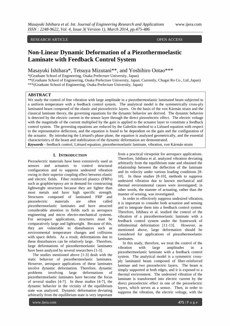
2.1 Problem

y

x

z

2h

2h

2b

2bao

:

2/0 hz

2/hz N

:

iz

1z

:

:

:

i

1

N

0

1iz

1Nz

1 sa kNk

sk

1 iN

Fig. 1: analytical model

The model under consideration is a simply supported

beam of dimensions hba and composed of N

layers, as shown in Fig. 1. The sk -th and ak -th

layers (ss kk zzz 1 ,

aa kk zzz 1 ) exhibit

piezoelectricity (with poling in the z or z

direction), while the other layers do not. The beam is

laminated in a symmetrical cross-ply manner.

The beam is subjected to temperature distributions

txT ,0 and txTN , on the upper 2hz and

lower 2hz surfaces, respectively, as thermal

disturbances that may vary with time t . Mechanical

disturbance is modeled as the combination of the

initial deflection and velocity.

To suppress the dynamic deformation due to the

disturbances, the beam is subjected to the feedback

control procedure: electric current tQs is detected in

the sk -th layer, which serves as a sensor to detect the

deformation due to the disturbances; electrical

potentials txak ,1 and tx

ak , determined on the

basis of tQs are applied to the upper 1

akzz and

lower akzz surfaces, respectively, of the ak -th

layer, which serves as an actuator to suppress the

deformation due to the disturbances. Moreover, in

order to suppress the deformation effectively, the

sensor and actuator are designed as a distributed

sensor and actuator [17], i.e., the width of the

electrodes for the sk and ak -th layers are variable as

xfbxb ss and xfbxb aa , respectively.

2.2 Governing Equations In this subsection, the fundamental equations which

govern the dynamic deformation of the beam are

presented.

Based on the classical laminate theory, the

displacements in the x and z directions are

expressed, respectively, as

txwwx

txwztxuu ,,

,,0

, (1)

where txu ,0 and txw , denote the displacements

on the central plane 0z . In order to treat

nonlinear deformation, the von Kármán strain is

introduced for the normal strain in the x direction as

2

2202

2

1

2

1

x

wz

x

w

x

u

x

w

x

uxx

. (2)

The electric field in the z direction is expressed by

the electric potential tzx ,, as

z

Ez

. (3)

Assuming xx , zD , and T denote the normal

stress in the x direction, the electric displacement in

the z direction, and the temperature distribution,

respectively, the constitutive equations for each layer

are given as

TEexPE iziixxixx , (4)

TpxPEexPD iizixxiiz , (5)

where iE , i , ie , i , and ip denote the elastic

modulus, permittivity, piezoelectric constant, stress-

temperature coefficient, and pyroelectric constant,

respectively, in the i -th layer, and

saii

kkkk

kikipe

ppeeasas

and0,0

,0,0. (6)

The function xPi takes values of +1 and -1 in the

portions with poling in the z and z directions,

respectively.

By substituting (2) into (4) and integrating without

and with multiplication with z, for 22 hzh we

have the constitutive equations of the laminated beam

as




E

x

T

xx

E

x

T

xx

MMx

wDM

NNx

w

x

uAN

2

2

20

,2

1

, (7)

where xN and xM denote the resultant force and

moment, respectively, defined by

2

2d,1,

h

hxxxx zzMN . (8)

T

xN and T

xM denote the thermally induced resultant

force and moment, respectively, per unit width

defined by

N

i

z

zi

T

x

T

x

i

i

zzTMN1

1

d,1, . (9)

E

xN and E

xM denote the electrically induced resultant

force and moment, respectively, per unit width. By

considering xfbxb ss and xfbxb aa ,

E

xN and E

xM are, respectively, defined by

sk

skss

ak

akaa

sk

skss

ak

akaa

sk

skss

ak

akaa

sk

skss

ak

akaa

z

zzksk

z

zzkak

z

z

szkk

z

z

azkk

E

x

z

zzksk

z

zzkak

z

z

szkk

z

z

azkk

E

x

zzEexfxP

zzEexfxP

zb

xbzEexP

zb

xbzEexPM

zEexfxP

zEexfxP

zb

xbEexP

zb

xbEexPN

1

1

1

1

1

1

1

1

d

d

d

d

,d

d

d

d

. (10)

From (10), it is found that xfxP aka and

xfxP aka, namely the profiles of poling directions

and widths of the electrodes, determine the effective

contribution of the electric field to the electrically

induced resultant force and moment. A and D

denote the extensional and bending rigidities,

respectively, defined by

N

i

z

zi

i

i

zzEDA1

2

1

d,1, . (11)

Equations of motion for the laminated beam are

given as

2

2

2

2

2

2

,0t

wh

x

wN

x

M

x

Nx

xx

, (12)

where is defined by

N

i

z

zi

i

i

zh 1

1

d1

, (13)

and denotes the mass density averaged along the

thickness direction.

By substituting (7) into (12), we have the equations

which govern displacements 0u and w as

2

2

2

2

0

22

2

0

1

,

,,

x

wNNMM

x

wuLt

wh

NNx

wuL

E

x

T

x

E

x

T

x

E

x

T

x

, (14)

where the definitions of differentiation operators 1L

and 2L are given as

4

4

2

2200

2

2

2

2

020

1

2

1,

,,

x

wD

x

w

x

w

x

uAwuL

x

w

x

w

x

uAwuL

. (15)

Because the beam is simply supported at both edges,

the mechanical boundary conditions are expressed as

axMwu x ,0;0,0,00 . (16)

The thermally induced resultant force and moment, T

xN and T

xM , and the electrically induced resultant

force and moment, E

xN and E

xM , must be determined

in order to solve (14). Assuming that the thickness of

the beam h is sufficiently small compared to its

length a , the temperature distribution is considered to

be linear with respect to the thickness direction, and it

is given as

txTtxTh

z

txTtxTtzxT

N

N

,,

,,2

1,,

0

0

. (17)

Substituting (17) into (9) gives

N

i

iiiN

T

x

N

i

iiiN

T

x

h

z

h

ztxTtxThM

h

z

h

ztxTtxThN

1

3

1

3

0

2

1

10

3

1,,

,,,2

1

.(18)

By assuming the thicknesses of the sk -th and ak -th

layers are sufficiently small compared to its length a ,

the electric field distributions in both layers are

considered to be linear with respect to the thickness

direction, and they are given as




aa

aa

a

aa

a

ss

ss

s

ss

s

kk

kk

k

kk

k

kk

kk

k

kk

k

zzz

zz

zztxtx

txtzx

zzz

zz

zztxtx

txtzx

1

1

1

1

1

1

1

1

1

1

:,,

,,,

;

:,,

,,,

. (19)

By substituting (3), (6), and (19) into (10), we have

2,,

2,,

,,,

,,

1

1

1

1

1

1

ss

sss

aa

aaa

sss

aaa

kk

kkk

ss

kk

kkk

aa

E

x

kkkss

kkkaa

E

x

zztxtxe

xfxP

zztxtxe

xfxPM

txtxexfxP

txtxexfxPN

, (20)

where akP and

skP are rewritten as aP and sP ,

respectively, for brevity.

In summary, (14) combined with (18) and (20) and

the boundary conditions expressed by (16) are the

equations that govern 0u and w , that is, the dynamic

deformation of the beam. Note that the applied

electric potentials txak ,1 and tx

ak , are

determined on the basis of the electric current tQs .

tQs reflects the dynamic deformation of the beam,

and the manner in which tQs reflects this dynamic

deformation is explained in the following subsection.

The procedures to determine txak ,1 and tx

ak ,

are provided in Subsection 2.5.

2.3 Sensor Equation

The detected electric current tQs is related to the

dynamic deformation of the beam through the direct

piezoelectric effect of the sensor layer. By

considering xfbxb ss , the electric charge tQs

is evaluated by

xxfbD

xxfbDtQ

a

szzz

a

szzzs

sk

sk

d

d2

1

0

0 1

. (21)

By substituting (2), (3), (5), (17), and (19) into (21),

differentiating the result with respect to t , and

applying the virtual short condition

txtxss kk ,, 1 , (22)

we have

xxfxbPtxTtxTh

zz

txTtxTp

x

wzz

x

w

x

w

x

ue

tQ

ssN

kk

Nk

a kk

k

s

ss

s

ss

s

d,,2

,,2

1

2

0

1

0

0 2

21

0

.(23)

It should be noted that tQs can be detected under

the virtual short condition of (22) by a current

amplifier [17], for example. Thus, the detected

electric current tQs is related to the dynamic

deformation of the beam.

2.4 Galerkin Method The Galerkin method [15] is used to solve (14) under

the condition described by (16) because (15) is a set

of simultaneous nonlinear partial differential

equations. Trigonometric functions are chosen as the

trial functions to satisfy (16), and the considered

displacements are expressed as the series

1

0 sin,,m

mmm xtwtuwu , (24)

where

a

mm

. (25)

Then, the Galerkin method is applied to (14) to obtain

,...,2,1

:0dsin

,

,0dsin,

2

2

0 2

20

22

2

0

0

1

m

xxx

wNN

MMx

wuLt

wh

xxNNx

wuL

m

E

x

T

x

aE

x

T

x

a

m

E

x

T

x

. (26)

Moreover, the distributions of temperature on both

surfaces of the beam and those of the electric potential

on both surfaces of the ak -th layer are assumed to be

uniform. Thus, one has

ttxttx

tTtxTtTtxT

aaaa kkkk

NN

,,,

,,,,

11

00. (27)

Substituting (22) and (27) into (18) and (20) gives

xfxPMM

xfxPNN

h

z

h

ztTtThM

h

z

h

ztTtThN

aa

E

x

E

x

aa

E

x

E

x

N

i

iiiN

T

x

N

i

iiiN

T

x

0,

0,

1

3

1

3

0

2

1

10

,

,3

1

,2

1

,(28)




where

2

,

1

10,

10,

aa

aaa

aaa

kk

kkk

E

x

kkk

E

x

zztteM

tteN

. (29)

In order to satisfy (16), T

xM and E

xM are evaluated

by using their Fourier series expansions as

1

,, sin,,m

m

E

mx

T

mx

E

x

T

x xtMtMMM , (30)

where tM T

mx, and tM E

mx, are given as

a

m

E

x

T

x

E

mx

T

mx xxMMa

tMtM0

,, dsin,2

, . (31)

Moreover, in order to construct a modal actuator [17],

the profiles of poling direction and the width of the

electrode in the ak -th layer are designed to be

xxfxPamaa sin . (32)

Then, from (28) and (32), one has

xMMxNNaa m

E

x

E

xm

E

x

E

x sin,sin 0,0, , (33)

from which it is found that the actuator induces the

am -th mode. By substituting (28) and (33) into (31),

we have

amm

E

x

E

mx

N

i

iii

N

T

mx

MtM

mmh

z

h

z

tTtThtM

0,,

1

3

1

3

0

2

,

,2,mod4

3

1. (34)

By substituting (15), (24), (25), (28), (30), and (33)

into (26), the simultaneous nonlinear equations with

respect to tum and twm are obtained as

,...,2,1

:

8

1

2

1

4

d

d

,04

2

1

0,,

2

1 1 1

,

2

1 1

2

1

,0,

2

22

2

2

0,

1 1

22

m

MM

wwwA

uwA

wN

wNDt

wh

N

wwuA

a

a

aa

mm

E

x

T

mxm

m i k

kimmmikckim

m l

lmlmmlm

m

mmmsm

E

xm

m

T

xmm

m

mm

E

xm

m i

immimimmm

, (35)

where the definitions of ij , ijk , ijks , , and ijklc, are

given in the previous paper [8]. Moreover, by

eliminating tum from (35), we obtain the

simultaneous nonlinear ordinary differential equations

with respect to twm ,,3,2,1 m as

,...,2,1

:

d

d

1 1 1

,

1

,2

22

m

pph

w

h

w

h

wk

h

wk

h

wk

h

w

th

A

mm

m i k

kimN

ikmm

m

mA

mmmmL

mm

a

,(36)

where

a

aa

a

aa

mm

E

xm

A

m

A

m

T

mxmmm

l

lmmikl

l

immikckim

N

ikmm

E

x

l l

lmlmmm

mmmsm

A

mmm

A

mmm

T

xmm

L

m

L

m

Mtpp

Mtpp

Ahk

Nh

tkk

NDhtkk

0,

2

,

2

1

,

23

,

0,

1

,

2

,,

22

,

,2

8

1

,2

4

,

.(37)

Moreover, in order to construct a modal sensor

[17], the profiles of poling direction and the width of

the electrode in the sk -th layer are designed to be

xxfxPsmss sin . (38)

From (23), (24), and (27), we have

s

sN

kk

Nk

mm

kk

m i

mimiimmc

m

mmmmks

m

mtTtT

h

zz

tTtTa

bp

wzz

ww

ua

betQ

ss

s

ss

ss

s

ss

2,mod

2

2

12

42

2

0

1

0

21

1 1

,

1

.(39)

Moreover, tum in (39) is eliminated using (35) to

give

s

sN

kk

Nk

mm

kk

m i

mimiimmc

l i k

kikilkikli

l

kilm

l

E

x

l

m

lmlmks

m

mtTtT

h

zz

tTtTa

bp

wzz

ww

ww

NA

abetQ

ss

s

ss

ss

s

s

a

ass

2,mod

2

2

12

42

2

412

0

1

0

21

1 1

,

1 1 1

1

0,

. ... (40)

In order to extract the fundamental physical

characteristics of the dynamic behavior of the beam,

the most fundamental mode is treated as

xtwwxtuu 1111

0 sin,sin . (41)




It should be noted that, from (25) and (41), tw1

denotes the deflection of the beam at its center. In

order to control the deformation described by (41), the

electrode on the actuator is designed as

1am . (42)

By considering (35) for 1m , one has

A

NAL

pp

h

wk

h

wkk

h

w

th

u

11

3

1111,1

111,11

1

2

22

1

d

d

,0

, (43)

where Lk1 , Ak 11,1 ,

Nk 1 1 1,1 , 1p , and Ap1 defined by (37)

are reduced, using Eqs. (41) and (42), to

E

x

AA

T

x

N

E

x

AA

T

x

LL

Mtpp

Mtpp

Ahk

Nhtkk

NDhtkk

0,

2

111

1,

2

111

4

1

3

111,1

0,

2

111,111,1

2

1

2

111

,

,8

1

,3

8

,

. (44)

Because the first mode is treated as in (41), the

electrode on the sensor is so designed that

1sm . (45)

Then, from (39) and (41), one has

tTtTh

zz

tTtTa

bp

wzz

wwa

betQ

N

kk

Nk

kk

ks

ss

s

ss

s

0

1

0

1

2

1

1

11

2

1

2

2

12

423

12

. (46)

2.5 Equation for Feedback Control In this subsection, we derive the equation to treat the

control of the free vibration of the beam exposed to

constant and uniform temperature.

We consider that the temperature on the upper and

lower surfaces of the beam is constant and uniform as

tTtTN 0 , (47)

which leads to

tzxT ,, , (48)

from (17), (27), and (47). From (28), (34), (46), and

(47), we have

0,0, , T

mx

T

xe

T

x MMhN , (49)

1

2

1

1

11

2

1423

12w

zzww

abetQ ss

s

kk

ks

, (50)

where

N

i

iiie

h

z

h

z

1

1 (51)

represents the stress-temperature coefficient averaged

with respect to the thickness direction.

We consider that the electric voltage applied to the

actuator, ttaa kk 1 , is designed to be

proportional to the electric current detected by the

sensor, tQs , as

tQGtt skk aa

1 , (52)

where G denotes the gain of the feedback control.

By substituting (29), (44), (49), and (52) into (43)

and (50), we have

psp

spe

ztQeGh

wAh

h

wtQehGhDh

h

w

th

2

1

3

1

4

1

3

12

1

2

1

2

1

1

2

22

8

3

8

d

d

, (53)

1

2

113

1

4

2wwz

abetQ pps

, (54)

where

22

,011

ssaa

sa

kkkk

pkkp

zzzzzeee

... (55)

and pz denotes the z coordinate of the central plane

of the actuator. The case of 0pz is treated for

brevity. By introducing the nondimensional

quantities as

GhA

abeAabhe

Q

hAI

hAAh

D

thA

h

z

h

wW

p

p

s

e

p

p

8

8,

8

,88

,8

,,

4

12

2

1

24

1

2

1

2

4

11

, (56)

(53) and (54) are nondimensionalized, respectively, as

pIWWIW

3

2

2

3

8

d

d, (57)

d

d

3

4

2

1 WWI p

. (58)

Thus, from (56)-(58), it is found that the

nondimensional deflection W and the

nondimensional electric current I are governed by

nondimensional parameters , p 210 p ,

and , which denote the rigidity reduced by

temperature, position of the actuator, and gain,

respectively. By substituting (58) into (57), we have

0

d

d

3

4

3

8

2

1

d

d

3

2

2

WW

WWW

Wpp

. (59)




It is found that (59) has a set of equilibrium solutions

0W , (60)

for 0 and

,0W , (61)

for 0 . Solutions described by (60) and (61) are

different in nature. In this study, we consider that the

temperature is lower than a critical value cr as

cr , (62)

where cr is defined by

h

D

e

2

1cr . (63)

From (56), (62), and (63), it is found that the

condition described by (62) leads to the condition

0 , (64)

which makes the linear rigidity in (59) positive. It

should be noted that the temperature described by (63)

is referred to as the buckling temperature.

In order to extract the governing parameters under

(64), nondimensional quantities are introduced as

pzt

Wx

16

3,,, , (65)

where x , t , , and z denote the nondimensional

quantities of the deflection, time, gain, and actuator's

position, respectively, and x , z , and t are different

from the coordinates and the time variable defined in

Subsection 2.1. Hereafter, x , z , and t are employed

in the sense of (65) for brevity. Then, (59) is

nondimensionalized as

0d

d,

d

d2

2

xgt

xzxf

t

x , (66)

where functions zxf , and xg are defined as

3

2,42

9

16, xxxgzxzxzxf

. (67)

The equation with the form of (66) is known as

Liénard's equation [16]. Particularly, if xg is

replaced with a linear function x and zxf , with a

symmetric function 12 x , (66) is referred to as van

der Pol equation. The cubic term in xg defined by

(67) is derived from the nonlinear term 2

2

x

wNx

in

(12) combined with (7). The function zxf , defined

by (67) is unsymmetric with respect to 0x because

the weight of the nonlinear term 2

2

x

wNx

in the left-

hand side of (12) is different from that of the

nonlinear term

2

2

1

x

w in the second and third terms

on the right-hand side of (2). In the context of this

research, the first, second, and third terms on the left-

hand side of (66) are the terms of inertia, damping,

and restoring force of the system, respectively.

From (66) and (67), it is found that (66) has its sole

equilibrium solution 0x . We call the function

zxf , as the damping characteristic function in the

sense that it describes the dependency of the damping

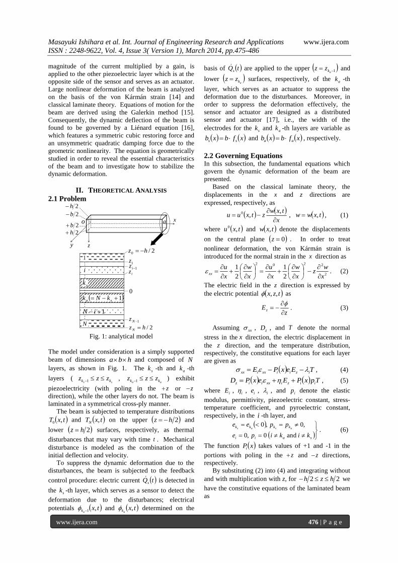
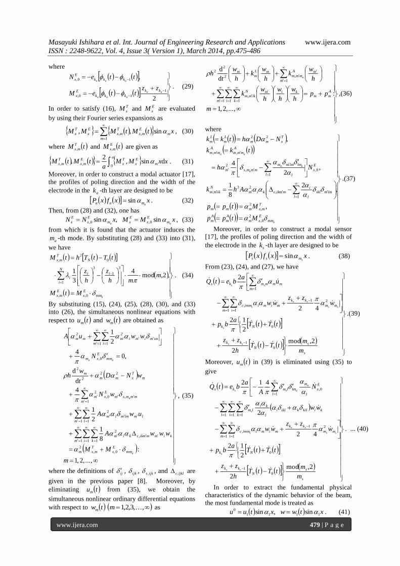
intensity for a deflection x . A numerical example of

the damping characteristic function zxf , is shown

in Fig. 2.

-0.2

-0.15

-0.1

-0.05

0

0.05

0.1

0.15

0.2

-1 -0.5 0 0.5 1 1.5x

zxf ,

Fig. 2: damping characteristic function

Because zxf , is positive in the vicinity of 0x , it

is found that the equilibrium solution 0x is locally

stable for 0 . Moreover, from (67) or Fig. 2, it is

found that

zxzzxf 42for0, . (68)

Therefore, the equilibrium solution 0x is expected

to be not only locally but also globally stable within a

certain range around 0x . Conversely, from (67) or

Fig. 2, it is found that

zxzxzxf 4or2for0, , (69)

which gives the system negative damping for 0 .

In that case, it is expected that a vibration with

relatively large amplitude will be unstable.

Therefore, it is important to determine the range of

deformation in which the system is operated stably.

For this purpose, the governing equation, (67), is

analyzed geometrically by introducing the Liénard's

phase plane [18] yx, that is governed by

xgyzxFyx

1

,, , (70)

where the overdot denotes differentiation with respect

to t , and zxF , is defined by

zxzxx

xzxfzxFx

2

3105

2

3105

27

16

d,,

2

0

. (71)

It should be noted that elimination of y in (70) leads

to the original governing equation, (67). From the

first part of (70), we have




zxFx

y ,

. (72)

Thus, we call y the modified velocity in the sense

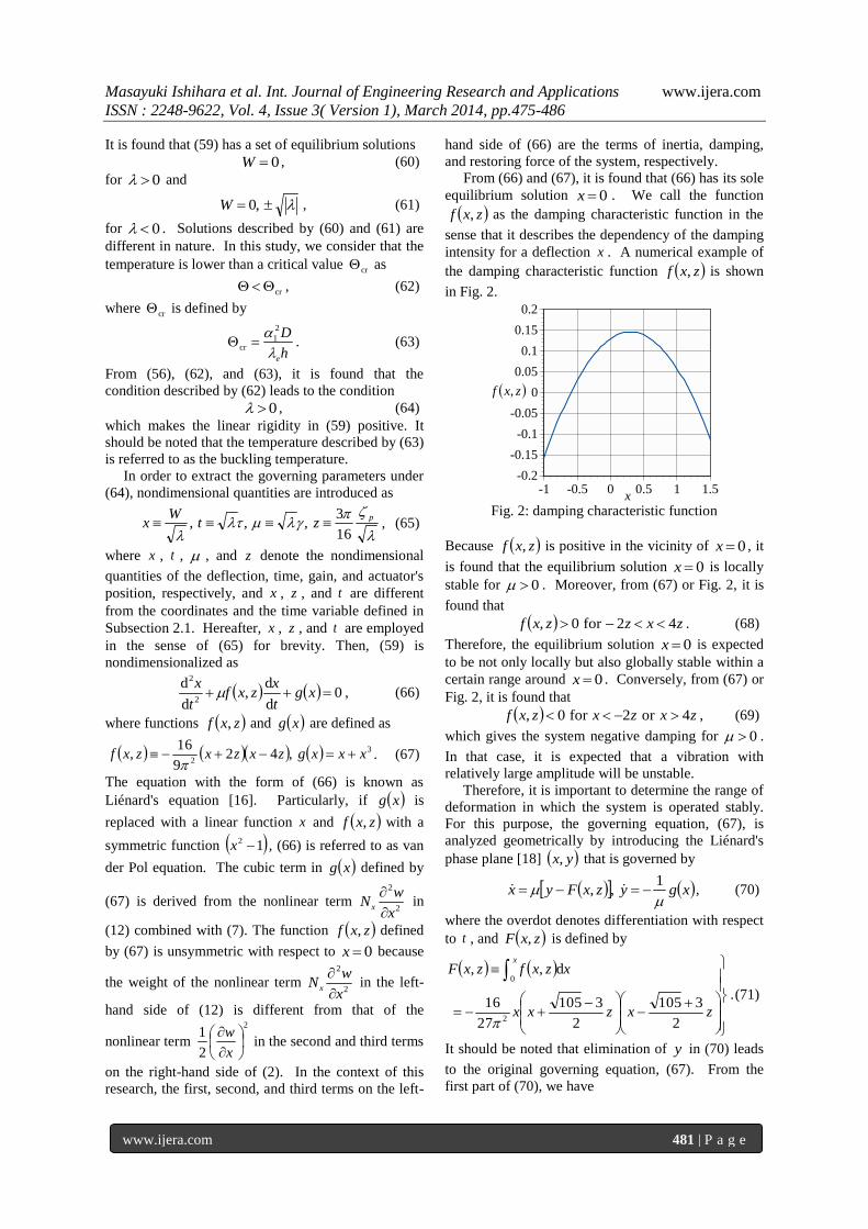
that it is related to the actual velocity x . Figure 3

shows the characteristics of the phase plane governed

by (70). The solid lines in red denote

zxFyx ,,0 , (73)

which make the right-hand sides of (70) null and are,

therefore, called nullclines. From (70), it is found that

the nullclines in (73) divide the phase plane shown in

Fig. 3 into four parts by the signs of x and y . The

broken arrows in Fig. 3 denote the directions of the

trajectories governed by (70). The examples of the

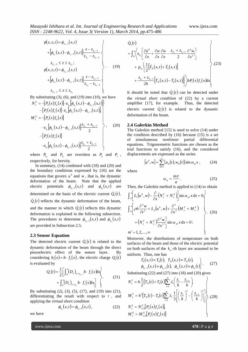
trajectories are indicated by blue lines in Fig. 4. The

point 00 , yx denotes the initial combination of yx, .

-4

-3

-2

-1

0

1

2

3

4

-4 -3 -2 -1 0 1 2 3 4x

y

0x zxFy ,

0,0 yx 0,0 yx

0,0 yx 0,0 yx

Fig. 3: characteristics of Liénard's phase plane

-0.8

-0.6

-0.4

-0.2

0

0.2

0.4

0.6

0.8

-2

-1.5 -1

-0.5 0

0.5 1

1.5 2

x

y

0,5.1, 00 yx

0,7.1, 00 yx

Fig. 4: examples of trajectories

From Fig. 4, it is found that a trajectory may move

toward or away from the equilibrium point

0,0, yx ; in other words, the vibration may be

stable or unstable. Therefore, it is expected that there

is a closed boundary line that divides the stability as

indicated by the broken line in Fig. 4. Such a line is

usually called the limit cycle. It should be noted that

the limit cycle is numerically obtained by changing

the variables as tt in (70) for an arbitrary initial

condition and, therefore, is dependent on parameters

and z .

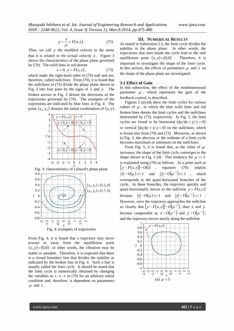
III. NUMERICAL RESULTS As stated in Subsection 2.5, the limit cycle divides the

stability in the phase plane. In other words, the

trajectories that start inside the cycle lead to the sole

equilibrium point 0,0, yx . Therefore, it is

important to investigate the shape of the limit cycle.

In this section, the effects of parameters and z on

the shape of the phase plane are investigated.

3.1 Effect of Gain In this subsection, the effect of the nondimensional

parameter , which represents the gain of the

feedback control, is described.

Figures 5 (a)-(d) show the limit cycles for various

values of , in which the blue solid lines and red

broken lines denote the limit cycles and the nullclines

determined by (73), respectively. In Fig. 5, the limit

cycles are found to be horizontal 0dd xyxy

or vertical 0dd yxyx on the nullclines, which

is found also from (70) and (73). Moreover, as shown

in Fig. 3, the abscissa or the ordinate of a limit cycle

becomes maximum or minimum on the nullclines.

From Fig. 5, it is found that, as the value of

increases, the shape of the limit cycle converges to the

shape shown in Fig. 5 (d). This tendency for 1

is explained using (70) as follows. At a point such as

1~, zxFy , equation (70) implies

1~ x and 1~ 1 y , which

corresponds to the quasi-horizontal branches of the

cycle. In these branches, the trajectory quickly and

quasi-horizontally moves to the nullcline zxFy ,

because 1~ x and 1~ 1 y .

However, once the trajectory approaches the nullcline

so closely that 2~, zxFy , then x and y

become comparable as 1~ x and 1~ y ,

and the trajectory moves nearly along the nullcline.

-1

-0.8

-0.6

-0.4

-0.2

0

0.2

0.4

0.6

0.8

1

-2.5 -2

-1.5 -1

-0.5 0

0.5 1

1.5 2

2.5

x

y

zxFy ,

(a) 5




-1

-0.8

-0.6

-0.4

-0.2

0

0.2

0.4

0.6

0.8

1

-2.5 -2

-1.5 -1

-0.5 0

0.5 1

1.5 2

2.5

x

y

zxFy ,

(b) 10

-1

-0.8

-0.6

-0.4

-0.2

0

0.2

0.4

0.6

0.8

1

-2.5 -2

-1.5 -1

-0.5 0

0.5 1

1.5 2

2.5

x

y

zxFy ,

(c) 20

-1

-0.8

-0.6

-0.4

-0.2

0

0.2

0.4

0.6

0.8

1

-2.5 -2

-1.5 -1

-0.5 0

0.5 1

1.5 2

2.5

x

y

zxFy ,

(d) 50

Fig. 5: effect of gain on limit cycle 3.0z

As x increases, y increases compared with x .

Therefore, the trajectory approaches the nullcline and

finally crosses the nullcline vertically, as shown in Fig.

3.

The maximum and minimum values of the abscissa

and ordinate of a limit cycle are important

characteristics of the cycle because they correspond to

the limit within which the system is operated safely.

To be more precise, the maximum and minimum

values of the abscissa correspond to the upper and

lower limits of the initial position when the initial

modified velocity is zero, and those of the ordinate

correspond to the upper and lower limits of the initial

modified velocity when the initial position is zero. In

view of these facts, we refer to the maximum and

minimum values of the abscissa of a limit cycle as the

upper and lower limits of the initial position,

respectively, and refer to those of the ordinate of the

cycle as the upper and lower limits of the initial

modified velocity, respectively. In addition, we refer

to the maximum and minimum values of the actual

velocity x along the limit cycle as the upper and

lower limits of the actual velocity, respectively.

Figure 6 shows the variations of the upper and

lower limits of the position, modified velocity, and

actual velocity with parameter , in which subscripts

“upper” and “lower” correspond to the upper and

lower limits, respectively. From Figs. 6 (a) and (b), it

is found that, as increases, the upper and lower

limits of the position and modified velocity change

monotonically and converge to certain values as

explained previously. From Fig. 6 (c), it is found that

the upper limit of the actual velocity increases as

increases and that the lower limit has a local

maximum.

Usually, a larger value of is preferable in order

to quickly pull the system back to the equilibrium

point 0,0, yx . However, as shown in lowerx in

Fig. 6 (a), the limit within which the system is

operated safely may decrease. In this regard, the safe

ranges of the initial position initialx , modified velocity

initialy , and actual velocity initialx are investigated.

From Fig. 6, it is found that the system is stable for an

arbitrary value of when initialx , initialy , and initialx

satisfies

01 upperinitiallower xxx , (74)

11 upperinitiallower yyy , (75)

and

013 upperinitiallower xxx , (76)

respectively.

-2

-1.5

-1

-0.5

0

0.5

1

1.5

2

2.5

0 10 20 30 40 50

lowerupper, xx

upperx

lowerx

(a) position




-5

-4

-3

-2

-1

0

1

2

3

4

5

0 10 20 30 40 50

lowerupper, yy

uppery

lowery

(b) modified velocity

-10

-5

0

5

10

15

0 10 20 30 40 50

lowerupper, xx

upperx

lowerx

(c) actual velocity

Fig. 6: variations of upper and lower limits with gain

3.0z

3.2 Effect of Actuator Position In this subsection, the effect of the nondimensional

parameter z , which represents the actuator position in

the laminated beam, is described.

-1

-0.8

-0.6

-0.4

-0.2

0

0.2

0.4

0.6

0.8

1

-2

-1.5 -1

-0.5 0

0.5 1

1.5 2

x

y

zxFy ,

(a) 1.0z

-1

-0.8

-0.6

-0.4

-0.2

0

0.2

0.4

0.6

0.8

1

-2

-1.5 -1

-0.5 0

0.5 1

1.5 2

x

y

zxFy ,

(b) 3.0z

-2

-1.5

-1

-0.5

0

0.5

1

1.5

2

-4 -3 -2 -1 0 1 2 3 4x

y

zxFy ,

(c) 5.0z

-4

-2

0

2

4

6

8

-12 -8 -4 0 4 8 12x

y

zxFy ,

(d) 1z

Fig. 7: effect of actuator position on limit cycle

10

Figures 7 (a)-(d) show the limit cycles for various

values of z , in which the blue solid lines and red

broken lines denote the limit cycles and the nullclines

determined by (73), respectively. Figures 8 (a), (b),

and (c) shows the variation of the upper and lower

limits of the position, modified velocity, and actual

velocity, respectively, with parameter z .




-6

-4

-2

0

2

4

6

8

0 0.2 0.4 0.6 0.8 1z

lowerupper, xx

upperx

lowerx

(a) position

-3

-2

-1

0

1

2

3

4

5

6

7

0 0.2 0.4 0.6 0.8 1z

lowerupper, yy uppery

lowery

(b) modified velocity

-30

-20

-10

0

10

20

30

40

50

60

70

0 0.2 0.4 0.6 0.8 1z

lowerupper, xx upperx

lowerx

(c) actual velocity

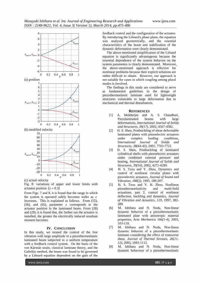
Fig. 8: variations of upper and lower limits with

actuator position 3.0z

From Figs. 7 and 8, it is found that the range in which

the system is operated safely becomes wider as z

increases. This is explained as follows. From (55),

(56), and (65), parameter z corresponds to the

actuator position in the laminated beam. From (28)

and (29), it is found that, the farther out the actuator is

installed, the greater the electrically induced resultant

moment becomes.

IV. CONCLUSION In this study, we treated the control of the free

vibration with large amplitude in a piezothermoelastic

laminated beam subjected to a uniform temperature

with a feedback control system. On the basis of the

von Kármán strain, classical laminate theory, and the

Galerkin method, the beam was found to be governed

by a Liénard equation dependent on the gain of the

feedback control and the configuration of the actuator.

By introducing the Liénard's phase plane, the equation

was analyzed geometrically, and the essential

characteristics of the beam and stabilization of the

dynamic deformation were clearly demonstrated.

The above-mentioned simplification of the Liénard

equation is significantly advantageous because the

essential dependence of the system behavior on the

system parameters is clearly demonstrated. Moreover,

the above-mentioned approach is effective for

nonlinear problems because their explicit solutions are

rather difficult to obtain. However, our approach is

not suitable for cases in which coupling among plural

modes is involved.

The findings in this study are considered to serve

as fundamental guidelines in the design of

piezothermoelastic laminate used for lightweight

structures vulnerable to large deformation due to

mechanical and thermal disturbances.

REFERENCES [1] A. Mukherjee and A. S. Chaudhuri,

Piezolaminated beams with large

deformations, International Journal of Solids

and Structures, 39(17), 2002, 4567-4582.

[2] H. S. Shen, Postbuckling of shear deformable

laminated plates with piezoelectric actuators

under complex loading conditions,

International Journal of Solids and

Structures, 38(44-45), 2001, 7703-7721.

[3] H. S. Shen, Postbuckling of laminated

cylindrical shells with piezoelectric actuators

under combined external pressure and

heating, International Journal of Solids and

Structures, 39(16), 2002, 4271-4289.

[4] H. S. Tzou and Y. Zhou, Dynamics and

control of nonlinear circular plates with

piezoelectric actuators, Journal of Sound and

Vibration, 188(2), 1995, 189-207.

[5] H. S. Tzou and Y. H. Zhou, Nonlinear

piezothermoelasticity and multi-field

actuations, part 2, control of nonlinear

deflection, buckling and dynamics, Journal

of Vibration and Acoustics, 119, 1997, 382-

389.

[6] M. Ishihara and N. Noda, Non-linear

dynamic behavior of a piezothermoelastic

laminated plate with anisotropic material

properties, Acta Mechanica 166(1-4), 2003,

103-118.


dynamic behavior of a piezothermoelastic

laminate considering the effect of transverse

shear, Journal of Thermal Stresses, 26(11-

12), 2003, 1093-1112.


dynamic behaviour of a piezothermoelastic




laminate, Philosophical Magazine 85(33-35),

2005, 4159-4179.

[9] Y. Watanabe, M. Ishihara, and N. Noda,

Nonlinear transient behavior of a

piezothermoelastic laminated beam

subjected to mechanical, thermal and

electrical load, Journal of Solid Mechanics

and Materials Engineering, 3(5), 2009, 758-

769.

[10] M. Ishihara, Y. Watanabe, and N. Noda,

Non-linear dynamic deformation of a

piezothermoelastic laminate, in H. Irschik, M.

Krommer, K. Watanabe, and T. Furukawa

(Ed.), Mechanics and model-based control of

smart materials and structures (Wien:

Springer-Verlag, 2010) 85-94.

[11] M. Ishihara, N. Noda, and H. Morishita,

Control of dynamic deformation of a

piezoelastic beam subjected to mechanical

disturbance by using a closed-loop control

system, Journal of Solid Mechanics and

Materials Engineering 1(7), 2007, 864-874.

[12] M. Ishihara, H. Morishita, and N. Noda,

Control of dynamic deformation of a

piezothermoelastic beam with a closed-loop

control system subjected to thermal

disturbance, Journal of Thermal Stresses,

30(9), 2007, 875-888.

[13] M. Ishihara, H. Morishita, and N. Noda,

Control of the transient deformation of a

piezoelastic beam with a closed-loop control

system subjected to mechanical disturbance

considering the effect of damping, Smart

Materials and Structures, 16(5), 2007, 1880-

1887.

[14] C. Y. Chia, Nonlinear analysis of plates

(New York: McGraw-Hill, 1980).

[15] C. A. J. Fletcher, Computational Galerkin

method (New York: Springer, 1984).

[16] S. H. Strogatz, Nonlinear dynamics and

chaos (Boulder: Westview Press, 2001).

[17] C. -K. Lee, Piezoelectric laminates: Theory

and experiments for distributed sensors and

actuators, in H. S. Tzou and G. L. Anderson

(Ed.), Intelligent Structural Systems

(Dordrecht: Kluwer Academic Publishers,

1992) 75-168.

[18] N. Minorsky, Nonlinear Oscillations

(Princeton: Van Nostrand, 1962).

Documents

Non-Linear Dynamic Deformation of a Piezothermoelastic ... 1/CH4301475486.pdf · Non-Linear Dynamic Deformation of a Piezothermoelastic Laminate with Feedback Control System Masayuki