Embed Size (px)
Citation preview
UNIVERSITÀ DEGLI STUDI DI PADOVAFACOLTÀ DI INGEGNERIA
CORSO DI LAUREA MAGISTRALE IN INGEGNERIA
DELL'AUTOMAZIONE
TESI DI LAUREA
NUMERICAL METHODS FOR MODEL
PREDICTIVE CONTROL
Laureando: GIANLUCA FRISON
Matricola: 620826
Relatore: Prof. MATTEO FISCHETTI
ANNO ACCADEMICO 2011-2012

Ringraziamenti
Vorrei ringraziare il mio relatore, Matteo Fischetti, per aver accettato di seguirmi,e per essere stato sempre estremamente disponibile nell'assecondare le mie limi-tate disponibilità di orari.
Vorrei anche ringraziare mio fratello Gabriele, per l'aiuto nella revisionelinguistica, e la mia ragazza Marie e tutta la mia famiglia, per il loro supportoe incoraggiamento.

ii
Summary
This thesis mainly deals with the extended linear quadratic control problem 2.1,that is a special case of equality constrained quadratic program. 2.1 is a verygeneral problem formulation, and it is useful for itself, since a number of otherproblems in optimal control and estimation of linear systems can be reducedto this form. Furthermore, it arises as sub-problem in sequential quadraticprograms methods and interior-point methods for the solution of optimal con-trol and estimation in case of non-linear systems and in presence of inequalityconstraints.
This thesis can be divided into two parts. In the �rst part, we present andanalyze a number of methods for the solution of problem 2.1. These methodshave been implemented in e�cient C code and compared each other.
In the second part, we de�ne problem 8.1, that is an extension of problem 2.1and takes into account also inequality constraints. Two interior-point methodsfor the solution of problem 8.1 are presented and analyzed. Both methods havebeen implemented in C code and compared each other.
The focus is on the �rst part: the main goal of this thesis is the e�cientimplementation and comparison of di�erent methods for solution of 2.1.

iv
Contents
Ringraziamenti i
Summary iii
Notation 1
1 Introduction 3
2 Extended Linear Quadratic Control Problem 5
2.1 De�nition . . . . . . . . . . . . . . . . . . . . . . . . . . . . . . . 52.1.1 Matrix form . . . . . . . . . . . . . . . . . . . . . . . . . . 6
2.2 Optimality conditions . . . . . . . . . . . . . . . . . . . . . . . . 72.2.1 KKT conditions . . . . . . . . . . . . . . . . . . . . . . . 72.2.2 Band diagonal representation of the KKT system . . . . . 13
3 Direct Sparse Solvers 15
3.1 MA57 . . . . . . . . . . . . . . . . . . . . . . . . . . . . . . . . . 153.2 PARDISO . . . . . . . . . . . . . . . . . . . . . . . . . . . . . . . 163.3 Performance analysis . . . . . . . . . . . . . . . . . . . . . . . . . 18
3.3.1 Cost of the di�erent parts of the solvers . . . . . . . . . . 183.3.2 Comparative test . . . . . . . . . . . . . . . . . . . . . . . 18
4 Schur Complement Method 21
4.1 Derivation . . . . . . . . . . . . . . . . . . . . . . . . . . . . . . . 214.2 Implemetation . . . . . . . . . . . . . . . . . . . . . . . . . . . . 234.3 Performance analysis . . . . . . . . . . . . . . . . . . . . . . . . . 27
4.3.1 Cost of sub-routines . . . . . . . . . . . . . . . . . . . . . 274.3.2 Comparative test . . . . . . . . . . . . . . . . . . . . . . . 30
5 Riccati Recursion Method 33
5.1 Derivation . . . . . . . . . . . . . . . . . . . . . . . . . . . . . . . 335.1.1 Derivation from the Cost Function Expression . . . . . . 335.1.2 Derivation using Dynamic Programming . . . . . . . . . . 395.1.3 Derivation from the KKT System . . . . . . . . . . . . . . 445.1.4 Properties of the Sequence Pn . . . . . . . . . . . . . . . . 47
vi CONTENTS
5.2 Implementation . . . . . . . . . . . . . . . . . . . . . . . . . . . . 49
5.2.1 Genaral form . . . . . . . . . . . . . . . . . . . . . . . . . 49
5.2.2 Form exploiting the symmetry of Pn . . . . . . . . . . . . 50
5.2.3 Form requiring Pn to be positive de�nite . . . . . . . . . 52
5.3 Performance analysis . . . . . . . . . . . . . . . . . . . . . . . . . 53
5.3.1 Cost of sub-routines . . . . . . . . . . . . . . . . . . . . . 53
5.3.2 Comparative test . . . . . . . . . . . . . . . . . . . . . . . 54
5.3.3 Conclusions . . . . . . . . . . . . . . . . . . . . . . . . . . 54
6 Condensing Methods 57
6.1 Derivation . . . . . . . . . . . . . . . . . . . . . . . . . . . . . . . 57
6.1.1 Null space method . . . . . . . . . . . . . . . . . . . . . . 57
6.1.2 State elimination . . . . . . . . . . . . . . . . . . . . . . . 61
6.2 Implementation . . . . . . . . . . . . . . . . . . . . . . . . . . . . 63
6.3 Performance analysis . . . . . . . . . . . . . . . . . . . . . . . . . 68
6.3.1 Cost of the di�erent parts of the algorithm . . . . . . . . 68
6.3.2 Cost of sub-routines . . . . . . . . . . . . . . . . . . . . . 69
6.3.3 Comparative test . . . . . . . . . . . . . . . . . . . . . . . 70
7 Test problems as Extended Linear Quadratic Control Problem 73
7.1 Mass-spring system . . . . . . . . . . . . . . . . . . . . . . . . . . 73
7.1.1 Problem de�nition . . . . . . . . . . . . . . . . . . . . . . 73
7.1.2 Small size example . . . . . . . . . . . . . . . . . . . . . . 76
7.2 Comparison tests . . . . . . . . . . . . . . . . . . . . . . . . . . . 79
7.2.1 Comparison in the solution of 2.1 on its own . . . . . . . 79
7.2.2 Comparison in the solution of 2.1 as subproblem in aninterior-point method . . . . . . . . . . . . . . . . . . . . 79
7.2.3 Comparison between the C and MATLAB implementa-tions of the same algorithm . . . . . . . . . . . . . . . . . 81
8 Extended Linear Quadratic Control Problem with Inequality
Constraints 85
8.1 De�nition . . . . . . . . . . . . . . . . . . . . . . . . . . . . . . . 85
8.1.1 Matrix From . . . . . . . . . . . . . . . . . . . . . . . . . 86
8.2 Optimality Conditions . . . . . . . . . . . . . . . . . . . . . . . . 86
9 Interior-point methods 91
9.1 Derivation . . . . . . . . . . . . . . . . . . . . . . . . . . . . . . . 91
9.1.1 Basic primal-dual method . . . . . . . . . . . . . . . . . . 91
9.1.2 Mehrotra's predictor-corrector method . . . . . . . . . . . 93
9.1.3 Computation of the steps as equality constrained quadraticprograms . . . . . . . . . . . . . . . . . . . . . . . . . . . 95
9.2 Implementation . . . . . . . . . . . . . . . . . . . . . . . . . . . . 97
9.2.1 Basic primal-dual method . . . . . . . . . . . . . . . . . . 97
9.2.2 Mehrotra's predictor-corrector method . . . . . . . . . . . 99
9.3 Performance analysis . . . . . . . . . . . . . . . . . . . . . . . . . 105
CONTENTS vii
10 Test Problems as Extended Linear Quadratic Control Problem
with Inequality Constraints 107
10.1 Problem de�nition . . . . . . . . . . . . . . . . . . . . . . . . . . 107
10.2 Small size example . . . . . . . . . . . . . . . . . . . . . . . . . . 108
10.3 Comparison between the two interior-point methods . . . . . . . 108
11 Problems variants 113
11.1 Variants of problem 2.2 . . . . . . . . . . . . . . . . . . . . . . . 113
11.1.1 Output in the cost function . . . . . . . . . . . . . . . . . 113
11.1.2 Input variation in the cost function . . . . . . . . . . . . . 114
11.1.3 Diagonal Hessian in the cost function . . . . . . . . . . . 116
11.2 Variants of problem 2.1 . . . . . . . . . . . . . . . . . . . . . . . 117
11.2.1 Control to a non-zero reference . . . . . . . . . . . . . . . 117
11.3 Variants of problem 8.1 . . . . . . . . . . . . . . . . . . . . . . . 117
11.3.1 Diagonal Hessian matrix in the cost function and box con-straints . . . . . . . . . . . . . . . . . . . . . . . . . . . . 117
12 Conclusions 119
A Machines and programming languages 121
A.1 Hardware and software . . . . . . . . . . . . . . . . . . . . . . . . 121
A.2 Programming languages . . . . . . . . . . . . . . . . . . . . . . . 122
A.2.1 MATLAB . . . . . . . . . . . . . . . . . . . . . . . . . . . 122
A.2.2 C . . . . . . . . . . . . . . . . . . . . . . . . . . . . . . . . 123
A.2.3 FORTRAN . . . . . . . . . . . . . . . . . . . . . . . . . . 123
B Basic Algorithms 125
B.1 Matrix-matrix multiplication . . . . . . . . . . . . . . . . . . . . 125
B.1.1 General matrices . . . . . . . . . . . . . . . . . . . . . . . 125
B.1.2 Triangular matrix . . . . . . . . . . . . . . . . . . . . . . 126
B.1.3 Rank-k update . . . . . . . . . . . . . . . . . . . . . . . . 126
B.1.4 Rank-n update with triangular matrices . . . . . . . . . . 126
B.2 Matrix-vector multiplication . . . . . . . . . . . . . . . . . . . . . 127
B.2.1 General matrix . . . . . . . . . . . . . . . . . . . . . . . . 128
B.2.2 Triangular matrix . . . . . . . . . . . . . . . . . . . . . . 128
B.3 Triangular solver . . . . . . . . . . . . . . . . . . . . . . . . . . . 128
B.3.1 Vector RHS . . . . . . . . . . . . . . . . . . . . . . . . . . 128
B.3.2 Matrix RHS . . . . . . . . . . . . . . . . . . . . . . . . . . 129
B.4 Cholesky factorization . . . . . . . . . . . . . . . . . . . . . . . . 129
B.5 Triangular matrix inversion . . . . . . . . . . . . . . . . . . . . . 132
C BLAS and LAPACK 133
C.1 BLAS . . . . . . . . . . . . . . . . . . . . . . . . . . . . . . . . . 133
C.1.1 Testing dgemm . . . . . . . . . . . . . . . . . . . . . . . . . 133
C.1.2 Testing dsyrk . . . . . . . . . . . . . . . . . . . . . . . . . 141
C.1.3 Testing dtrmm . . . . . . . . . . . . . . . . . . . . . . . . . 142
C.1.4 Testing dtrsm . . . . . . . . . . . . . . . . . . . . . . . . . 143
C.2 LAPACK . . . . . . . . . . . . . . . . . . . . . . . . . . . . . . . 144
C.2.1 Testing dpotrf . . . . . . . . . . . . . . . . . . . . . . . . 144
viii CONTENTS
D Time tables 149
D.1 Direct sparse solvers . . . . . . . . . . . . . . . . . . . . . . . . . 149D.2 Schur complement method . . . . . . . . . . . . . . . . . . . . . . 151D.3 Riccati recursion . . . . . . . . . . . . . . . . . . . . . . . . . . . 153D.4 Condensing methods . . . . . . . . . . . . . . . . . . . . . . . . . 156D.5 Comparison between C and MATLAB code . . . . . . . . . . . . 159D.6 Interior-point methods . . . . . . . . . . . . . . . . . . . . . . . . 161
Bibliography 163
Notation
In this thesis we use the following notation:
• matrices are written with capital letters, e.g. A; vectors and scalars arewritten in small letters, e.g. x, α.
• the transpose of A is indicated as A′.
• the gradient of φ(x, u) with respect to the vector u is indicated as ∇uφ.
• the minimizer of the cost function φ(x) is indicated as x∗.
• the integer n is used as index for loops over the control horizon, n ∈{0, 1, . . . , N}; the integer k is used as index for iterations of interior-pointmethods. The same notation is used for the relative subscripts.
In the algorithms, we use the following notation:
• with {Qn} we mean the set of matrices {Q0, Q1, . . . , QN}; similarly forvectors.
• the notation {xn}k indicates the set of vectors {x0, x1, . . . xN} at the k-thiteration of an interior-point method; in order to keep the notation easier,sometimes we use the notation xk instead.
• the notation x(0:n−1) indicates the sub-vector of the vector x with indexesbetween 0 and n− 1 both inclusive.
• the notation A(n,0:n−1) indicates the elements on the n-th row of the ma-trix A, with column indexes between 0 and n− 1 both inclusive.
• in the algorithms for the solution of problem 2.1, a sub-script in romanstyle indicates the BLAS or LAPACK routine used to perform the oper-ation, e.g. C ← A ·dgemm B means that the matrix C gets the result ofthe product between the matrices A and B, computed using the BLASroutine dgemm.

2 CONTENTS
Chapter 1
Introduction
This thesis deals mainly with a sub-problem often arising in model predictivecontrol, namely the extended linear quadratic control problem
minun,xn+1
φ =
N−1∑n=0
ln(xn, un) + lN (xN )
s.t. xn+1 = Anxn +Bnun + bn
(1.1)
where n ∈ {0, 1, . . . , N − 1} and
ln(xn, un) =1
2
[x′n u′n
] [ Qn S′nSn Rn
] [xnun
]+[q′n s′n
] [ xnun
]+ ρn
lN (xN ) =1
2x′NQNxN + q′NxN + ρN
From a mathematical point of view, problem 1.1 is an equality constrainedquadratic program.
Our work consists in a theoretical study of a number of well known methodsfor the solution of 1.1 and in the following e�cient implementation in C code.
The main contribution of our work consists in the systematic presentationof existing methods, and on the comparison of their e�cient implementationsin terms of equally optimized C code.
The structure of this thesis is the following:
• This chapter, chapter 1, introduces the central argument and the structureof this thesis.
• Chapter 2 introduces problem 1.1 and presents necessary and su�cientconditions for its solution. It is shown how the solution of 1.1 can befound solving a linear system of equations (the KKT system).
• Chapter 3 brie�y presents and compares two direct sparse solvers for thesolution of the KKT system associated with problem 1.1.
4 Introduction
• Chapters 4 to 6 present a number of methods for the solution of 1.1,one for chapter. Each chapter contains the theoretical derivation of therelative method in at least one way, the e�cient implementation, and theperformance analysis in terms of number of �oating-point operations anduse of sub-routines.
• Chapter 7 states and analyzes a test problem, and compares the methodsderived in the previous chapters in terms of execution time. Two seriesof tests are performed: in the �rst one the methods are compared inthe solution of problem 1.1 on its own; in the second one the methodsare compared in the solution of problem 1.1 as sub-problem in an interior-point method, avoiding the re-computation of quantities that are constantamong iterations.
• Chapter 8 introduces problem 8.1, that is an extension of problem 1.1 in-cluding also inequality constraints (and thus deals with an general quadraticprogram, with both equality and inequality constraints). Both necessaryand su�cient conditions for its solution are derived. It is shown how thesolution of 8.1 can be found solving a system of non-linear equations (theKKT system for a general quadratic program).
• Chapter 9 presents two interior-point methods for the solution of 8.1: themethods are derived in the case of a general quadratic program, thenthe implementation is tailored in the case of problem 8.1. Methods per-formance is compared in terms of �oating-point operations per iteration.An important result in this chapter is the fact that problem 1.1 arises assub-problem in interior-point methods for the solution of problem 8.1.
• Chapter 10 states a test problem for problem 8.1 compares the behaviorof the two interior-point methods.
• Chapter 11 presents a few problems related to 1.1 and 8.1, and shows howto tailor the methods presented in previous chapters to fully exploit thespecial structure of these problems.
• Chapter 12 contains some brief conclusions.
• Appendix A brie�y introduces the hardware and the software used to writethe code and test it.
• Appendix B presents some useful algorithms performing basic linear al-gebra operations, and states their complexity as number of �oating-pointoperations. The BLAS or LAPACK routines implementing the di�erentmethods are brie�y described.
• Appendix C presents and tests a number of implementations of the BLASand LAPACK libraries.
• Finally, appendix D contains tables collecting data from numerical tests.
Chapter 2
Extended Linear Quadratic
Control Problem
In this chapter we present the problem we mainly deal with, namely the extendedlinear quadratic control problem. We also derive necessary and su�cient condi-tions for its solution, and show that the solution can be found solving a systemof linear equations (KKT system).
2.1 De�nition
The extended linear quadratic control problem can be used to represent a num-ber of problems in optimal control and estimation of linear systems. It is alsoa subproblem in sequential quadratic programming methods and interior-pointmethods for non-linear and constrained optimal control and estimation: exam-ples can be found in [JGND12].
The extended linear quadratic control problem is de�ned as
Problem 1. The extended linear quadratic control problem is the equality con-
strained quadratic program
minun,xn+1
φ =
N−1∑n=0
ln(xn, un) + lN (xN )
s.t. xn+1 = Anxn +Bnun + bn
(2.1)
where n ∈ {0, 1, . . . , N − 1} and
ln(xn, un) =1
2
[x′n u′n
] [ Qn S′nSn Rn
] [xnun
]+[q′n s′n
] [ xnun
]+ ρn
lN (xN ) =1
2x′NQNxN + q′NxN + ρN
6 Extended Linear Quadratic Control Problem
In the above problem de�nition, the dynamic system model is linear (orbetter a�ne) time variant, and that the cost function is quadratic, with weightsmatrices time variant as well.
Problem 2.1 is an extension of the standard linear quadratic control problem,de�ned as
Problem 2. The standard linear quadratic control problem is the equality con-
strained quadratic program
minun,xn+1
φ =1
2
N−1∑k=0
[x′n u′n
] [ Q S′
S R
] [xnun
]+
1
2x′NQNxN
s.t. xn+1 = Axn +Bun
(2.2)
where n ∈ {0, 1, . . . , N − 1}.
In this problem de�nition the dynamic system model is strictly linear andtime invariant, and the cost function is strictly quadratic and time invariant.
This work focuses on the extended linear quadratic control problem 2.1, anddeals with the most e�cient methods to solve it. Problem 2.2 is a special case ofproblem 2.1, and thus can be solved using the methods derived for the latter. Itis also possible to tailor the algorithms in order to exploit the simpler structureand obtain better performances.
2.1.1 Matrix form
From a mathematical point of view, the extended linear quadratic control prob-lem is an equality constrained quadratic program. It can be rewritten in a morecompact form as
minx
φ =1
2x′Hx+ g′x
s.t. Ax = b(2.3)
where the state vector is
x =
u0
x1
u1
...xN−1
uN−1
xN
and the matrices relative to the cost function and the constraints are
H =
R0
Q1 S′1S1 R1
. . .
QN−1 S′N−1
SN−1 RN−1
QN
, g =
S0x0 + s0
q1
s1
...qN−1
sN−1
qN
2.2 Optimality conditions 7
A =
−B0 I
−A1 −B1 I. . .
. . .
−AN−1 −BN−1 I
, b =
A0x0 + b0
b1...
bN−1
.The matrices H and A are large, sparse and highly structured: this structurecan be exploited to obtain e�cient algorithms.
Note In 2.3, the cost function does not contain a constant term, even if 2.1does. The constant term does not in�uence the position of the minimum butonly its value, and we are interested only in the �rst: then we prefer to dropthe constant term, to keep the notation easier.
2.2 Optimality conditions
In the �rst part of this section we present necessary and su�cient conditionsfor the solution of a general equality constrained quadratic program; later wederive conditions for the speci�c case of the extended linear quadratic controlproblem 2.1, exploiting the special form of this problem.
2.2.1 KKT conditions
Here we present �rst order necessary optimality condition, known as Karush-Kuhn-Tucker (brie�y KKT) conditions, for x∗ to be a solution of a generalequality constrained quadratic program. For the general theory, see [NW06]
The Lagrangian function associated to a general equality constrained quadraticprogram in the form 2.3 takes the form
L = L(x, π) = φ− π′(Ax− b) =1
2x′Hx+ g′x− π′(Ax− b).
In the special case of problem 2.1 it takes the form
L(x, π) =1
2x′Hx+ g′x− π′(Ax− b) =
=
N−1∑n=0
ln(xn, un) + lN (xN )−N−1∑n=0
π′n+1(xn+1 −Anxn −Bnun − bn)
where
π =
π1
π2
...πN
is the vector of the the Lagrangian multipliers associated to the N constraintsAx− b = 0.
The �rst order necessary conditions for optimality (known as KKT condi-tions) can be found setting to zero the gradients of the Lagrangian function withrespect to the vectors x and π,
∇xφ(x, π) =Hx+ g −A′π = 0 (2.4a)
∇πφ(x, π) =Ax− b = 0. (2.4b)
8 Extended Linear Quadratic Control Problem
The conditions are stated in the proposition:
Proposition 1 (First order necessary conditions). If x∗ is a solution of the
equality constrained quadratic program, then there exists a vector π∗ such that
Hx∗ + g −A′π∗ = 0 and Ax∗ − b = 0.
Proof. We immediately notice that condition 2.4b is the equality constraintsequation: if x∗ does not satisfy this condition, it can not be a solution since itdoes not satisfy the constraints.
Thus, let x∗ be a solution: x∗ is a point satisfying the constraints Ax∗+b = 0and is a global minimizer for the cost function in the feasible region de�ned bythe constraints, i.e. for each x satisfying the constraints Ax + b = 0 we haveφ(x∗) ≤ φ(x).
We notice that, if the point x∗ is on the constraints, given any other point xon the constraint we have that the step ∆x = x−x∗ satis�es A∆x = Ax−Ax∗ =b − b = 0, and thus a general vector along the constraint is in the kernel (ornull space) of the matrix A, and thus it is in the image of the null space matrixZ. The matrix Z is de�ned as the matrix with full column rank whose columnsgenerate the null space of A; this implies AZ = 0.
The geometric interpretation of condition 2.4a is that the gradient of the costfunction in x∗ is orthogonal to the constraints. In fact the �rst condition canbe rewritten as Hx∗ + g = A′π∗, that means that the vector Hx∗ + g is in theimage of the matrix A′, Hx∗ + g ∈ Im(A′). The relation1 Ker(A) = Im(A′)⊥
implies that (Hx∗ + g) ⊥ Ker(A).Now we want to show that, if condition 2.4a is false, then it is always possible
to �nd a step ∆x along the constraint and such that φ(x∗ + ∆x) < φ(x∗): inparticular, the step in the direction de�ned by the projection on the vector spacegenerated by the matrix Z of the opposite of the gradient of the cost functioncomputed in x∗ makes the job.
Let us suppose that condition 2.4a is false, this means (Hx∗+ g) 6⊥ Ker(A),and then there exist a vector z ∈ Ker(A) such that (Hx∗ + g)′z 6= 0. Thisimplies that the projection of the gradient on the null space of the matrix A isnot zero, (Hx∗ + g)′Z 6= 0, and then also y = −(Hx∗ + g)′Z 6= 0. The vector yis a vector in the null space of A: its expression in the larger space is Zy; thisis not the zero vector since y 6= 0 and Z ha full column rank.
As step we choose the scaled vector
∆x = (Zy)λ = ZZ ′(Hx∗ + g)(−λ)
with the scalar λ > 0. The point x = x∗ + ∆x satis�es the constraint, sinceAx = Ax∗ +AZyλ = b+ 0 = b, and the value of the cost function in x is
φ(x) =φ(x∗ + ∆x) =1
2(x∗)′Hx∗ + g′x∗ +
1
2∆x′H∆x+ (Hx∗ + g)′∆x =
=φ(x∗) +1
2λy′Z ′HZyλ− (Hx∗ + g)′ZZ ′(Hx∗ + g)λ =
=φ(x∗) +1
2αλ2 − βλ.
1This relation can be proved in this way: if we use the notation < vi > to denote thevector space generated by the vectors vi, we have that Im(A′) =< coli(A
′) >, where coli(A′)is the i-th column of the matrix A′. We can now prove that Ker(A) = {x|Ax = 0} = {x|x ⊥rowi(A)} = {x|x ⊥ coli(A′)} =< coli(A
′) >⊥= Im(A′)⊥.
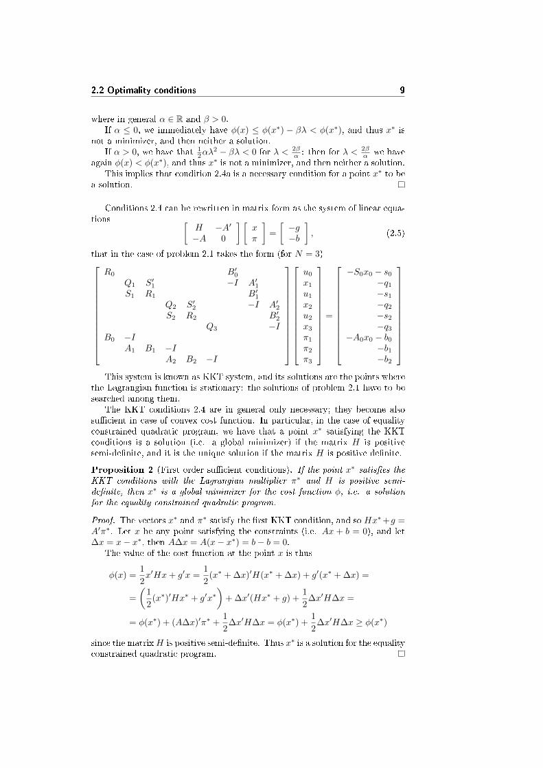
2.2 Optimality conditions 9
where in general α ∈ R and β > 0.If α ≤ 0, we immediately have φ(x) ≤ φ(x∗) − βλ < φ(x∗), and thus x∗ is
not a minimizer, and then neither a solution.If α > 0, we have that 1
2αλ2 − βλ < 0 for λ < 2β
α : then for λ < 2βα we have
again φ(x) < φ(x∗), and thus x∗ is not a minimizer, and then neither a solution.This implies that condition 2.4a is a necessary condition for a point x∗ to be
a solution.
Conditions 2.4 can be rewritten in matrix form as the system of linear equa-tions [
H −A′−A 0
] [xπ
]=
[−g−b
], (2.5)
that in the case of problem 2.1 takes the form (for N = 3)
R0 B′0Q1 S′1 −I A′1S1 R1 B′1
Q2 S′2 −I A′2S2 R2 B′2
Q3 −IB0 −I
A1 B1 −IA2 B2 −I
u0
x1
u1
x2
u2
x3
π1
π2
π3
=
−S0x0 − s0
−q1
−s1
−q2
−s2
−q3
−A0x0 − b0−b1−b2
This system is known as KKT system, and its solutions are the points where
the Lagrangian function is stationary: the solutions of problem 2.1 have to besearched among them.
The KKT conditions 2.4 are in general only necessary; they become alsosu�cient in case of convex cost function. In particular, in the case of equalityconstrained quadratic program, we have that a point x∗ satisfying the KKTconditions is a solution (i.e. a global minimizer) if the matrix H is positivesemi-de�nite, and it is the unique solution if the matrix H is positive de�nite.
Proposition 2 (First order su�cient conditions). If the point x∗ satis�es theKKT conditions with the Lagrangian multiplier π∗ and H is positive semi-
de�nite, then x∗ is a global minimizer for the cost function φ, i.e. a solution
for the equality constrained quadratic program.
Proof. The vectors x∗ and π∗ satisfy the �rst KKT condition, and so Hx∗+g =A′π∗. Let x be any point satisfying the constraints (i.e. Ax + b = 0), and let∆x = x− x∗, then A∆x = A(x− x∗) = b− b = 0.
The value of the cost function at the point x is thus
φ(x) =1
2x′Hx+ g′x =
1
2(x∗ + ∆x)′H(x∗ + ∆x) + g′(x∗ + ∆x) =
=
(1
2(x∗)′Hx∗ + g′x∗
)+ ∆x′(Hx∗ + g) +
1
2∆x′H∆x =
= φ(x∗) + (A∆x)′π∗ +1
2∆x′H∆x = φ(x∗) +
1
2∆x′H∆x ≥ φ(x∗)
since the matrixH is positive semi-de�nite. Thus x∗ is a solution for the equalityconstrained quadratic program.
10 Extended Linear Quadratic Control Problem
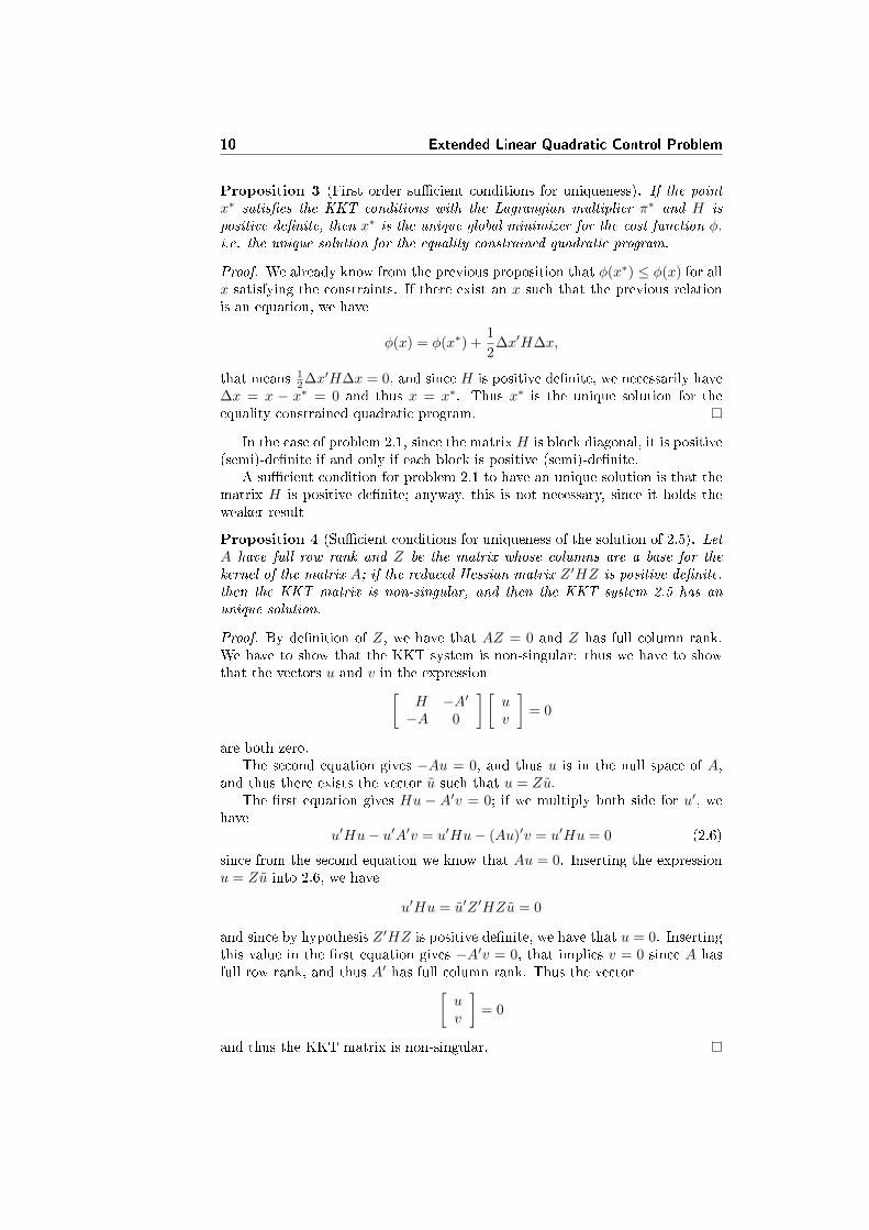
Proposition 3 (First order su�cient conditions for uniqueness). If the point
x∗ satis�es the KKT conditions with the Lagrangian multiplier π∗ and H is
positive de�nite, then x∗ is the unique global minimizer for the cost function φ,i.e. the unique solution for the equality constrained quadratic program.
Proof. We already know from the previous proposition that φ(x∗) ≤ φ(x) for allx satisfying the constraints. If there exist an x such that the previous relationis an equation, we have
φ(x) = φ(x∗) +1
2∆x′H∆x,
that means 12∆x′H∆x = 0, and since H is positive de�nite, we necessarily have
∆x = x − x∗ = 0 and thus x = x∗. Thus x∗ is the unique solution for theequality constrained quadratic program.
In the case of problem 2.1, since the matrix H is block diagonal, it is positive(semi)-de�nite if and only if each block is positive (semi)-de�nite.
A su�cient condition for problem 2.1 to have an unique solution is that thematrix H is positive de�nite; anyway, this is not necessary, since it holds theweaker result
Proposition 4 (Su�cient conditions for uniqueness of the solution of 2.5). LetA have full row rank and Z be the matrix whose columns are a base for the
kernel of the matrix A; if the reduced Hessian matrix Z ′HZ is positive de�nite,
then the KKT matrix is non-singular, and then the KKT system 2.5 has an
unique solution.
Proof. By de�nition of Z, we have that AZ = 0 and Z has full column rank.We have to show that the KKT system is non-singular: thus we have to showthat the vectors u and v in the expression[
H −A′−A 0
] [uv
]= 0
are both zero.The second equation gives −Au = 0, and thus u is in the null space of A,
and thus there exists the vector u such that u = Zu.The �rst equation gives Hu − A′v = 0; if we multiply both side for u′, we
haveu′Hu− u′A′v = u′Hu− (Au)′v = u′Hu = 0 (2.6)
since from the second equation we know that Au = 0. Inserting the expressionu = Zu into 2.6, we have
u′Hu = u′Z ′HZu = 0
and since by hypothesis Z ′HZ is positive de�nite, we have that u = 0. Insertingthis value in the �rst equation gives −A′v = 0, that implies v = 0 since A hasfull row rank, and thus A′ has full column rank. Thus the vector[
uv
]= 0
and thus the KKT matrix is non-singular.
2.2 Optimality conditions 11
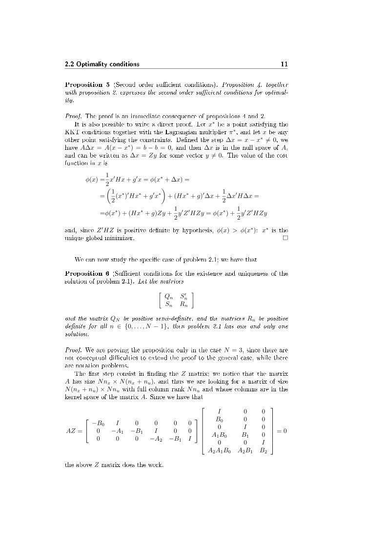
Proposition 5 (Second order su�cient conditions). Proposition 4, together
with proposition 2, expresses the second order su�cient conditions for optimal-
ity.
Proof. The proof is an immediate consequence of propositions 4 and 2.
It is also possible to write a direct proof. Let x∗ be a point satisfying theKKT conditions together with the Lagrangian multiplier π∗, and let x be anyother point satisfying the constraints. De�ned the step ∆x = x − x∗ 6= 0, wehave A∆x = A(x − x∗) = b − b = 0, and then ∆x is in the null space of A,and can be written as ∆x = Zy for some vector y 6= 0. The value of the costfunction in x is
φ(x) =1
2x′Hx+ g′x = φ(x∗ + ∆x) =
=
(1
2(x∗)′Hx∗ + g′x∗
)+ (Hx∗ + g)′∆x+
1
2∆x′H∆x =
=φ(x∗) + (Hx∗ + g)Zy +1
2y′Z ′HZy = φ(x∗) +
1
2y′Z ′HZy
and, since Z ′HZ is positive de�nite by hypothesis, φ(x) > φ(x∗): x∗ is theunique global minimizer.
We can now study the speci�c case of problem 2.1; we have that
Proposition 6 (Su�cient conditions for the existence and uniqueness of thesolution of problem 2.1). Let the matrices[
Qn S′nSn Rn
]and the matrix QN be positive semi-de�nite, and the matrices Rn be positive
de�nite for all n ∈ {0, . . . , N − 1}, then problem 2.1 has one and only one
solution.
Proof. We are proving the proposition only in the case N = 3, since there arenot conceptual di�culties to extend the proof to the general case, while thereare notation problems.
The �rst step consist in �nding the Z matrix; we notice that the matrixA has size Nnx × N(nx + nu), and thus we are looking for a matrix of sizeN(nx + nu) × Nnu with full column rank Nnu and whose columns are in thekernel space of the matrix A. Since we have that
AZ =
−B0 I 0 0 0 00 −A1 −B1 I 0 00 0 0 −A2 −B1 I
I 0 0B0 0 00 I 0
A1B0 B1 00 0 I
A2A1B0 A2B1 B2
= 0
the above Z matrix does the work.
12 Extended Linear Quadratic Control Problem
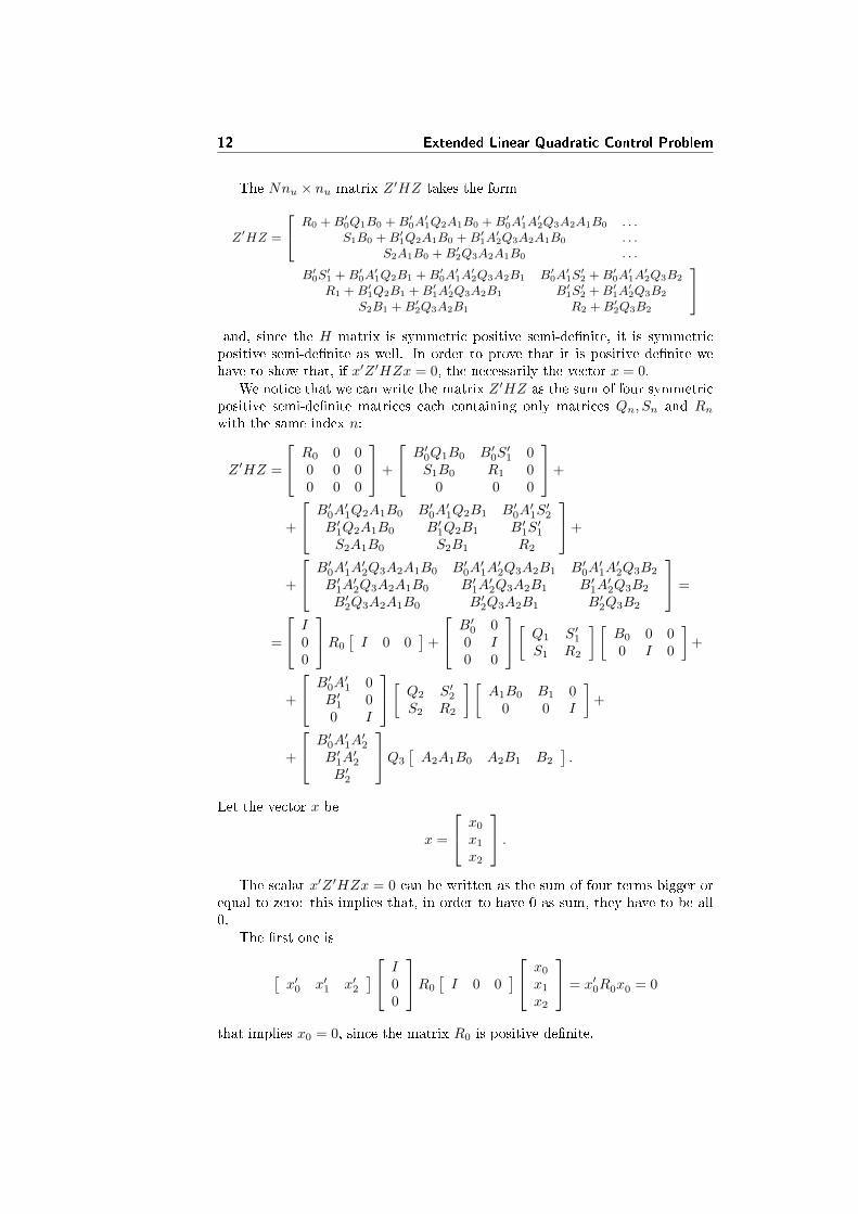
The Nnu × nu matrix Z ′HZ takes the form
Z′HZ =
R0 +B′0Q1B0 +B′0A′1Q2A1B0 +B′0A
′1A′2Q3A2A1B0 . . .
S1B0 +B′1Q2A1B0 +B′1A′2Q3A2A1B0 . . .
S2A1B0 +B′2Q3A2A1B0 . . .
B′0S′1 +B′0A
′1Q2B1 +B′0A
′1A′2Q3A2B1 B′0A
′1S′2 +B′0A
′1A′2Q3B2
R1 +B′1Q2B1 +B′1A′2Q3A2B1 B′1S
′2 +B′1A
′2Q3B2
S2B1 +B′2Q3A2B1 R2 +B′2Q3B2
and, since the H matrix is symmetric positive semi-de�nite, it is symmetricpositive semi-de�nite as well. In order to prove that it is positive de�nite wehave to show that, if x′Z ′HZx = 0, the necessarily the vector x = 0.
We notice that we can write the matrix Z ′HZ as the sum of four symmetricpositive semi-de�nite matrices each containing only matrices Qn, Sn and Rnwith the same index n:
Z ′HZ =
R0 0 00 0 00 0 0
+
B′0Q1B0 B′0S′1 0
S1B0 R1 00 0 0
+
+
B′0A′1Q2A1B0 B′0A
′1Q2B1 B′0A
′1S′2
B′1Q2A1B0 B′1Q2B1 B′1S′1
S2A1B0 S2B1 R2
+
+
B′0A′1A′2Q3A2A1B0 B′0A
′1A′2Q3A2B1 B′0A
′1A′2Q3B2
B′1A′2Q3A2A1B0 B′1A
′2Q3A2B1 B′1A
′2Q3B2
B′2Q3A2A1B0 B′2Q3A2B1 B′2Q3B2
=
=
I00
R0
[I 0 0
]+
B′0 00 I0 0
[ Q1 S′1S1 R2
] [B0 0 00 I 0
]+
+
B′0A′1 0
B′1 00 I
[ Q2 S′2S2 R2
] [A1B0 B1 0
0 0 I
]+
+
B′0A′1A′2
B′1A′2
B′2
Q3
[A2A1B0 A2B1 B2
].
Let the vector x be
x =
x0
x1
x2
.The scalar x′Z ′HZx = 0 can be written as the sum of four terms bigger or
equal to zero: this implies that, in order to have 0 as sum, they have to be all0.
The �rst one is
[x′0 x′1 x′2
] I00
R0
[I 0 0
] x0
x1
x2
= x′0R0x0 = 0
that implies x0 = 0, since the matrix R0 is positive de�nite.
2.2 Optimality conditions 13
The second one is
[0 x′1 x′2
] B′0 00 I0 0
[ Q1 S′1S1 R2
] [B0 0 00 I 0
] 0x1
x2
= x′1R1x1 = 0
that implies x1 = 0, since the matrix R1 is positive de�nite.The third one is
[0 0 x′2
] B′0A′1 0
B′1 00 I
[ Q2 S′2S2 R2
] [A1B0 B1 0
0 0 I
] 00x2
= x′2R2x2 = 0
that implies x2 = 0, since the matrix R2 is positive de�nite.In this way the whole vector x = 0, and so the matrix Z ′HZ is positive
de�nite, and by proposition 5 this means that problem 2.1 has one and only onesolution.
Note (Symmetry) Even if it is not necessary for the proof of the previous
proposition, it is usually requested to the matrices R0,
[Qn S′nSn Rn
]and QN
to be also symmetric: this would lead to more e�cient algorithms; on the otherhand, this is not a limitation, since it is always possible to rewrite a positivesemi-de�nite matrix in an equivalent symmetric form.
In what follows we assume that the above matrices are all symmetric.
2.2.2 Band diagonal representation of the KKT system
The KKT system of problem 2.1 can be written as
R0 B′0B0 −I
−I Q1 S′1 A′1S1 R1 B′1A1 B1 −I
−I Q2 S′2 A′2S2 R2 B′2A2 B2 −I
−I Q3
u0
π1
x1
u1
π2
x2
u2
π3
x3
=
−S0x0 − s0
−A0x0 − b0−q1
−s1
−b1−q2
−s2
−b2−q3
(2.7)
The advantage of this form is that the KKT system is represented in banddiagonal form, with band width depending on nx and nu but independent of N :this implies that the system can be solved in time O(N(nx + nu)3) (where nxis the length of the x vector and nu is the length of the u vector), using a banddiagonal generic solver. As a comparison, the solution of 2.7 by means of the useof a dense LDL′ factorization requires roughly 1
3 (N(2nx + nu))3 �oating-pointoperations.
This representation will also be useful in chapter 5 about the Riccati, sinceit is possible to derive the Riccati recursion method as a block solution strategyfor this system.

14 Extended Linear Quadratic Control Problem
Chapter 3
Direct Sparse Solvers
In this chapter we directly solve the KKT system 2.7 using direct sparse solvers.The system is large and sparse, and can be written in a band diagonal form,with a bandwidth depending only on nx and nu and not on N : the solvers areable to exploit this structure, and �nd the solution in a time of the order ofN(nx + nu)3.
We investigate the solvers MA57 and PARDISO, two of the best solvers forthe solution of sparse symmetric linear systems. We present the two solvers inbrief; the reader can �nd more information consulting the relative web-sites orliterature, for example [Duf04] and [SG11].
3.1 MA57
MA57 is a direct solver for symmetric sparse systems of linear equations; it ispart of HSL1 software.
It is designed to solve the linear system of equations
AX = B
where the n × n matrix A is large sparse and symmetric, and not necessarilyde�nite, and the right-hand side B may have more that one column. Thealgorithm performs an LDL′ factorization of the matrix A, implemented usinga multi-frontal approach.
The solver uses the BLAS library to perform matrix-vector and matrix-matrix operations: this means it can exploit a BLAS implementation optimizedfor the speci�c architecture. It also uses (optionally) the MeTiS library, per-forming partitioning of graphs.
The code consists in a number of routines; the one of interest for us are:
1HSL, a collection of Fortran codes for large-scale scienti�c computation. Seehttp://www.hsl.rl.ac.uk/
16 Direct Sparse Solvers
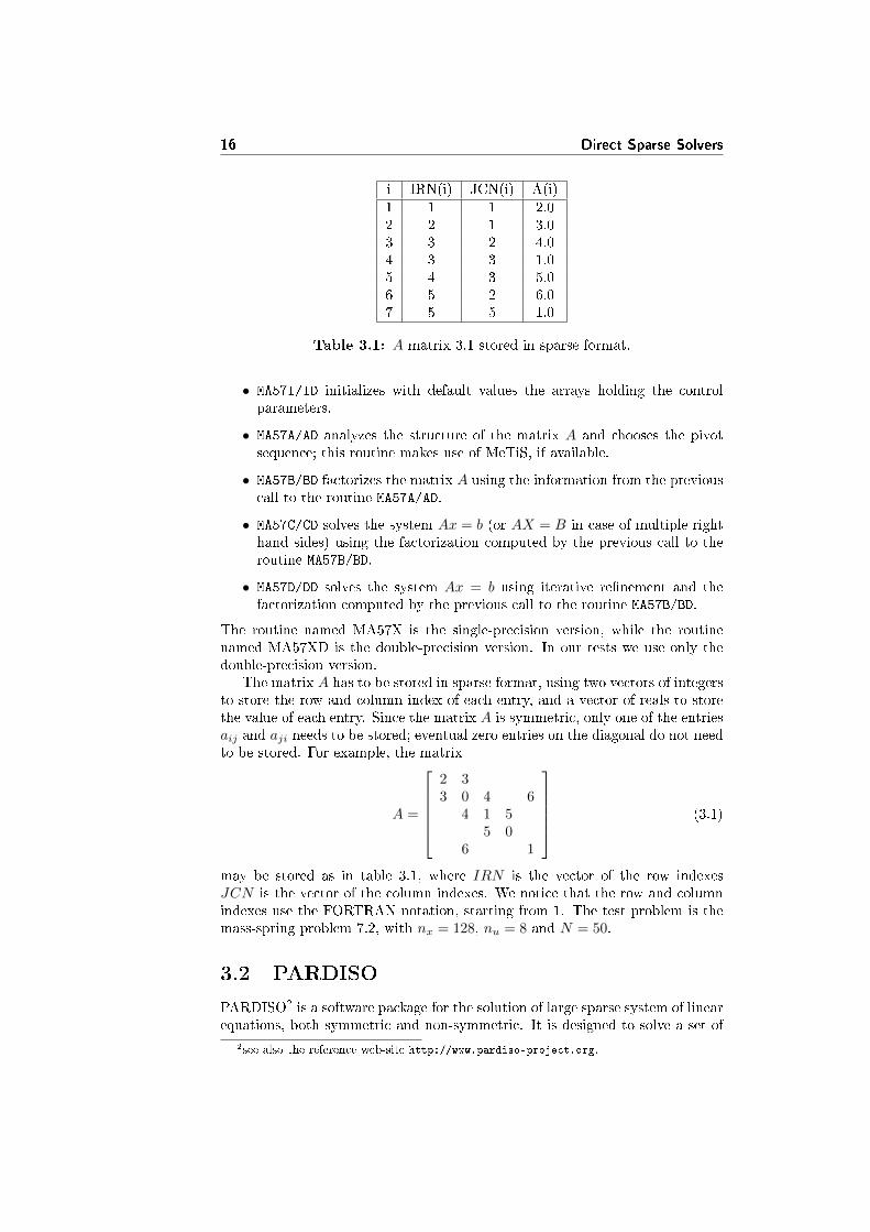
i IRN(i) JCN(i) A(i)1 1 1 2.02 2 1 3.03 3 2 4.04 3 3 1.05 4 3 5.06 5 2 6.07 5 5 1.0
Table 3.1: A matrix 3.1 stored in sparse format.
• MA57I/ID initializes with default values the arrays holding the controlparameters.
• MA57A/AD analyzes the structure of the matrix A and chooses the pivotsequence; this routine makes use of MeTiS, if available.
• MA57B/BD factorizes the matrix A using the information from the previouscall to the routine MA57A/AD.
• MA57C/CD solves the system Ax = b (or AX = B in case of multiple righthand sides) using the factorization computed by the previous call to theroutine MA57B/BD.
• MA57D/DD solves the system Ax = b using iterative re�nement and thefactorization computed by the previous call to the routine MA57B/BD.
The routine named MA57X is the single-precision version, while the routinenamed MA57XD is the double-precision version. In our tests we use only thedouble-precision version.
The matrix A has to be stored in sparse format, using two vectors of integersto store the row and column index of each entry, and a vector of reals to storethe value of each entry. Since the matrix A is symmetric, only one of the entriesaij and aji needs to be stored; eventual zero entries on the diagonal do not needto be stored. For example, the matrix
A =
2 33 0 4 6
4 1 55 0
6 1
(3.1)
may be stored as in table 3.1, where IRN is the vector of the row indexesJCN is the vector of the column indexes. We notice that the row and columnindexes use the FORTRAN notation, starting from 1. The test problem is themass-spring problem 7.2, with nx = 128, nu = 8 and N = 50.
3.2 PARDISO
PARDISO2 is a software package for the solution of large sparse system of linearequations, both symmetric and non-symmetric. It is designed to solve a set of
2see also the reference web-site http://www.pardiso-project.org.
3.2 PARDISO 17
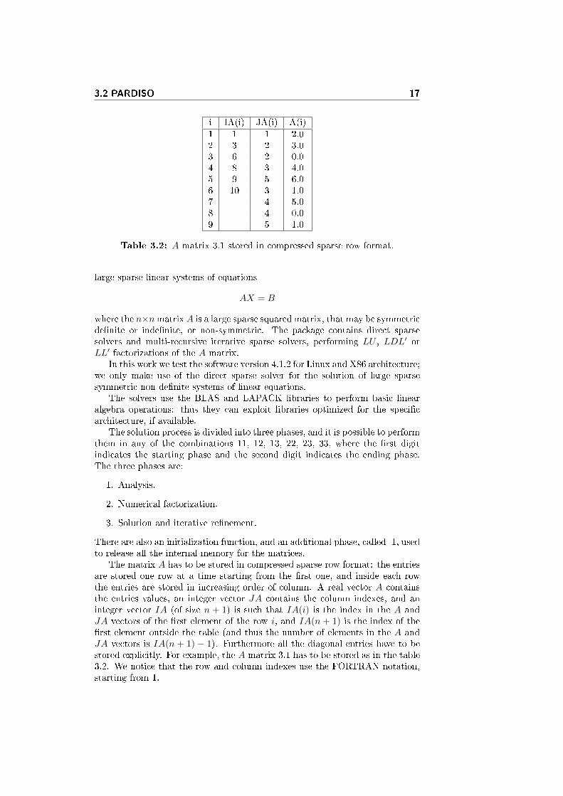
i IA(i) JA(i) A(i)1 1 1 2.02 3 2 3.03 6 2 0.04 8 3 4.05 9 5 6.06 10 3 1.07 4 5.08 4 0.09 5 1.0
Table 3.2: A matrix 3.1 stored in compressed sparse row format.
large sparse linear systems of equations
AX = B
where the n×nmatrixA is a large sparse squared matrix, that may be symmetricde�nite or inde�nite, or non-symmetric. The package contains direct sparsesolvers and multi-recursive iterative sparse solvers, performing LU , LDL′ orLL′ factorizations of the A matrix.
In this work we test the software version 4.1.2 for Linux and X86 architecture;we only make use of the direct sparse solver for the solution of large sparsesymmetric non-de�nite systems of linear equations.
The solvers use the BLAS and LAPACK libraries to perform basic linearalgebra operations: thus they can exploit libraries optimized for the speci�carchitecture, if available.
The solution process is divided into three phases, and it is possible to performthem in any of the combinations 11, 12, 13, 22, 23, 33, where the �rst digitindicates the starting phase and the second digit indicates the ending phase.The three phases are:
1. Analysis.
2. Numerical factorization.
3. Solution and iterative re�nement.
There are also an initialization function, and an additional phase, called -1, usedto release all the internal memory for the matrices.
The matrix A has to be stored in compressed sparse row format: the entriesare stored one row at a time starting from the �rst one, and inside each rowthe entries are stored in increasing order of column. A real vector A containsthe entries values, an integer vector JA contains the column indexes, and aninteger vector IA (of size n + 1) is such that IA(i) is the index in the A andJA vectors of the �rst element of the row i, and IA(n + 1) is the index of the�rst element outside the table (and thus the number of elements in the A andJA vectors is IA(n + 1) − 1). Furthermore all the diagonal entries have to bestored explicitly. For example, the A matrix 3.1 has to be stored as in the table3.2. We notice that the row and column indexes use the FORTRAN notation,starting from 1.
18 Direct Sparse Solvers
MA57 PARDISOphase time (s) % time (s) %
create A and B 0.033544 4.7 0.026609 0.8initialization 0.000012 0.0 0.001402 0.0analysis 0.133541 18.7 2.081128 65.8
factorization 0.534067 74.6 0.975534 30.9solution 0.014367 2.0 0.076888 2.4
total 0.715531 100.0 3.161561 99.9
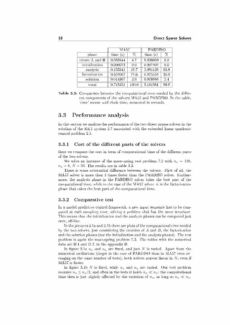
Table 3.3: Comparison between the computational time needed by the di�er-ent components of the solvers MA57 and PARDISO. In the table,'time' means wall clock time, measured in seconds.
3.3 Performance analysis
In this section we analyze the performance of the two direct sparse solvers in thesolution of the KKT system 2.7 associated with the extended linear quadraticcontrol problem 2.1.
3.3.1 Cost of the di�erent parts of the solvers
Here we compare the cost in term of computational time of the di�erent partsof the two solvers.
We solve an instance of the mass-spring test problem 7.2 with nx = 128,nu = 8, N = 50. The results are in table 3.3.
There is some substantial di�erence between the solvers. First of all, theMA57 solver is more than 4 times faster than the PARDISO solver. Further-more, the analysis phase in the PARDISO solver takes the best part of thecomputational time, while in the case of the MA57 solver, it is the factorizationphase that takes the best part of the computational time.
3.3.2 Comparative test
In a model predictive control framework, a new input sequence has to be com-puted at each sampling time, solving a problem that has the same structure.This means that the initialization and the analysis phases can be computed justonce, o�-line.
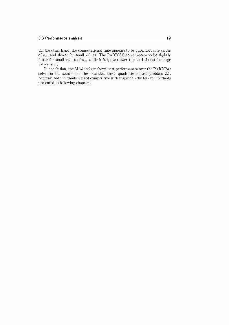
In the pictures 3.1a and 3.1b there are plots of the computational time neededby the two solvers, just considering the creation of A and B, the factorizationand the solution phases (not the initialization and the analysis phases). The testproblem is again the mass-spring problem 7.2. The tables with the numericaldata are D.1 and D.2, in the appendix D.
In �gure 3.1a nx and nu are �xed, and just N is varied. Apart from thenumerical oscillations (larger in the case of PARDISO than in MA57 even av-eraging on the same number of tests), both solvers appear linear in N , even ifMA57 is faster.
In �gure 3.1b N is �xed, while nx and nu are varied. Our test problemrequires nu ≤ nx/2, and often in the tests it holds nu � nx: the computationaltime then is just slightly a�ected by the variation of nu, as long as nu � nx.
3.3 Performance analysis 19
On the other hand, the computational time appears to be cubic for large valuesof nx, and slower for small values. The PARDISO solver seems to be slightlyfaster for small values of nx, while it is quite slower (up to 4 times) for largevalues of nx.
In conclusion, the MA57 solver shows best performances over the PARDISOsolver in the solution of the extended linear quadratic control problem 2.1.Anyway, both methods are not competitive with respect to the tailored methodspresented in following chapters.
20 Direct Sparse Solvers
10 20 30 40 50 60 70 80 90 1000
0.05
0.1
0.15
0.2
0.25
0.3
0.35
0.4
nx=50, n
u=5
N
wa
ll clo
ck tim
e (
s)
PARDISO
MA57
(a) nx = 50 and nu = 5 �xed, N varied.
0.5 1 1.5 2 2.5 3−5
−4
−3
−2
−1
0
1
2
3N=10
log10
(nx)
log
10(w
all
clo
ck t
ime
)
n
x
3
PARDISO, nu=1
PARDISO, nu=2
PARDISO, nu=4
PARDISO, nu=8
MA57, nu=1
MA57, nu=2
MA57, nu=4
MA57, nu=8
(b) N = 10 �xed, nx ∈ {4, 8, 16, 32, 64, 128, 256, 512} and nu ∈ {1, 2, 4, 8}varied.
Figure 3.1: Comparison of the performance of the solvers PARDISO andMA57 in the solution of the problem 2.1, using as test problemthe mass-spring problem 7.2.
Chapter 4
Schur Complement Method
The KKT system 2.7 may be solved even by using the Schur complement of theKKT matrix. This approach is producing matrices whose non-zero elementsare all around the diagonal, packed into sub-matrices. Thus the sparsity of theKKT matrix is preserved. Furthermore, it is possible to work just on the densesub-matrices, using the standard BLAS and LAPACK routines. The drawbackof this approach is the need for the Hessian matrix H to be positive de�niteinstead of just positive semi-de�nite. The method has the same asymptoticcomplexity as the direct sparse solvers in chapter 3, namely N(nx + nu)3, butit is faster in practice.
4.1 Derivation
This section is divided into two parts: in the �rst part we derive the Schurcomplement method for the solution of a general equality constrained quadraticprogram. In the second part we specialize the method in the case of problem2.1.
General case
The use of the Schur complement method for the solution of the general equalityconstrained quadratic program is discussed in [NW06].
We consider the KKT system of the general equality constrained quadraticprogram 2.3, that is in the form[
H −A′−A 0
] [xπ
]= −
[gb
]. (4.1)
We can rewrite 4.1 in the equivalent form{Hx−A′π = −g−Ax = −b
(4.2)
22 Schur Complement Method
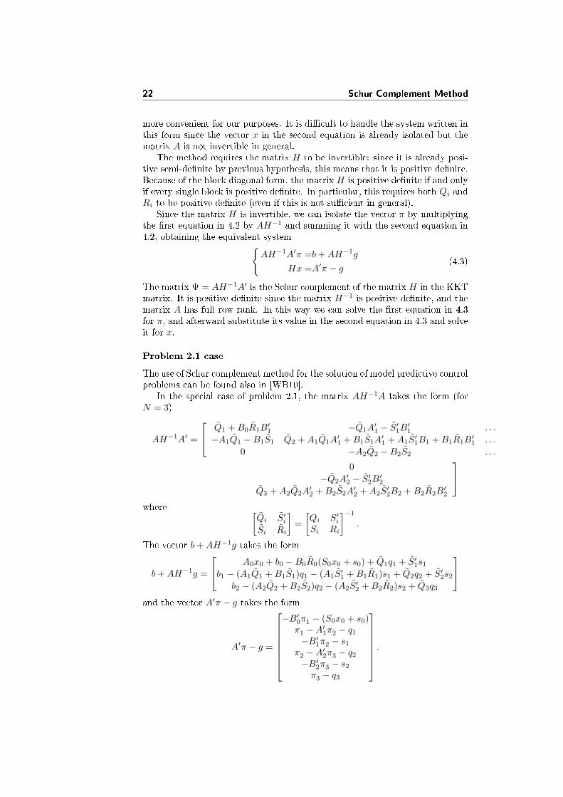
more convenient for our purposes. It is di�cult to handle the system written inthis form since the vector x in the second equation is already isolated but thematrix A is not invertible in general.
The method requires the matrix H to be invertible: since it is already posi-tive semi-de�nite by previous hypothesis, this means that it is positive de�nite.Because of the block diagonal form, the matrix H is positive de�nite if and onlyif every single block is positive de�nite. In particular, this requires both Qi andRi to be positive de�nite (even if this is not su�cient in general).
Since the matrix H is invertible, we can isolate the vector π by multiplyingthe �rst equation in 4.2 by AH−1 and summing it with the second equation in4.2, obtaining the equivalent system{
AH−1A′π =b+AH−1g
Hx =A′π − g(4.3)
The matrix Ψ = AH−1A′ is the Schur complement of the matrix H in the KKTmatrix. It is positive de�nite since the matrix H−1 is positive de�nite, and thematrix A has full row rank. In this way we can solve the �rst equation in 4.3for π, and afterward substitute its value in the second equation in 4.3 and solveit for x.
Problem 2.1 case
The use of Schur complement method for the solution of model predictive controlproblems can be found also in [WB10].
In the special case of problem 2.1, the matrix AH−1A takes the form (forN = 3)
AH−1A′ =
Q1 +B0R1B′1 −Q1A
′1 − S′1B′1 . . .
−A1Q1 −B1S1 Q2 +A1Q1A′1 +B1S1A
′1 +A1S
′1B1 +B1R1B
′1 . . .
0 −A2Q2 −B2S2 . . .
0
−Q2A′2 − S′2B′2
Q3 +A2Q2A′2 +B2S2A
′2 +A2S
′2B2 +B2R2B
′2
where [
Qi S′iSi Ri
]=
[Qi S′iSi Ri
]−1
.
The vector b+AH−1g takes the form
b+AH−1g =
A0x0 + b0 −B0R0(S0x0 + s0) + Q1q1 + S′1s1
b1 − (A1Q1 +B1S1)q1 − (A1S′1 +B1R1)s1 + Q2q2 + S′2s2
b2 − (A2Q2 +B2S2)q2 − (A2S′2 +B2R2)s2 + Q3q3
and the vector A′π − g takes the form
A′π − g =
−B′0π1 − (S0x0 + s0)
π1 −A′1π2 − q1
−B′1π2 − s1
π2 −A′2π3 − q2
−B′2π3 − s2
π3 − q3
.
4.2 Implemetation 23
4.2 Implemetation
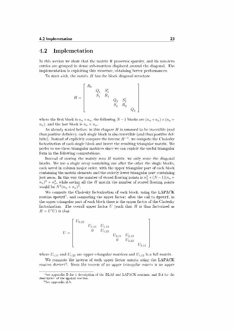
In this section we show that the matrix Ψ preserves sparsity, and its non-zeroentries are grouped in dense sub-matrices displaced around the diagonal. Theimplementation is exploiting this structure, obtaining better performances.
To start with, the matrix H has the block diagonal structure
H =
R0
Q1 S′1S1 R1
Q2 S′2S2 R2
Q3
where the �rst block is nu×nu, the following N−1 blocks are (nu+nx)× (nu+nx), and the last block is nx × nx.
As already stated before, in this chapter H is assumed to be invertible (andthus positive de�nite): each single block is also invertible (and thus positive def-inite). Instead of explicitly compute the inverse H−1, we compute the Choleskyfactorization of each single block and invert the resulting triangular matrix. Weprefer to use these triangular matrices since we can exploit the useful triangularform in the following computations.
Instead of storing the mainly zero H matrix, we only store the diagonalblocks. We use a single array containing one after the other the single blocks,each saved in column-major order, with the upper triangular part of each blockcontaining the matrix elements and the strictly lower triangular part containingjust zeros. In this way the number of stored �oating points is n2
u+(N −1)(nu+nx)2 + n2
x, while saving all the H matrix the number of stored �oating pointswould be N2(nu + nx)2.
We compute the Cholesky factorization of each block, using the LAPACKroutine dpotrf1, and computing the upper factor: after the call to dpotrf, inthe upper triangular part of each block there is the upper factor of the Choleskyfactorization. The overall upper factor U (such that H is thus factorized asH = U ′U) is thus
U =
U0,22
U1,11 U1,12
0 U1,22
U2,11 U2,12
0 U2,22
U3,11
where Ui,11 and Ui,22 are upper triangular matrices and Ui,12 is a full matrix.
We compute the inverse of each upper factor matrix using the LAPACKroutine dtrtri2. Since the inverse of an upper triangular matrix is an upper
1See appendix B for a description of the BLAS and LAPACK routines, and B.4 for thedescription of the dpotrf routine.
2See appendix B.5.
24 Schur Complement Method
triangular matrix, the inverse U−1 of the U matrix is
U−1 =
U0,22
U1,11 U1,12
0 U1,22
U2,11 U2,12
0 U2,22
U3,11
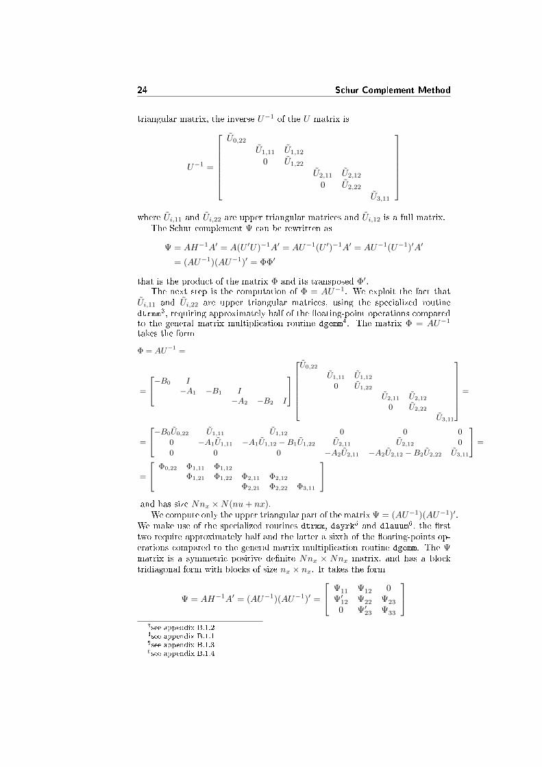
where Ui,11 and Ui,22 are upper triangular matrices and Ui,12 is a full matrix.
The Schur complement Ψ can be rewritten as
Ψ = AH−1A′ = A(U ′U)−1A′ = AU−1(U ′)−1A′ = AU−1(U−1)′A′
= (AU−1)(AU−1)′ = ΦΦ′
that is the product of the matrix Φ and its transposed Φ′.The next step is the computation of Φ = AU−1. We exploit the fact that
Ui,11 and Ui,22 are upper triangular matrices, using the specialized routinedtrmm3, requiring approximately half of the �oating-point operations comparedto the general matrix multiplication routine dgemm4. The matrix Φ = AU−1
takes the form
Φ = AU−1 =
=
−B0 I−A1 −B1 I
−A2 −B2 I
U0,22
U1,11 U1,12
0 U1,22
U2,11 U2,12
0 U2,22
U3,11
=
=
−B0U0,22 U1,11 U1,12 0 0 0
0 −A1U1,11 −A1U1,12 −B1U1,22 U2,11 U2,12 0
0 0 0 −A2U2,11 −A2U2,12 −B2U2,22 U3,11
=
=
Φ0,22 Φ1,11 Φ1,12
Φ1,21 Φ1,22 Φ2,11 Φ2,12
Φ2,21 Φ2,22 Φ3,11
and has size Nnx ×N(nu+ nx).
We compute only the upper triangular part of the matrix Ψ = (AU−1)(AU−1)′.We make use of the specialized routines dtrmm, dsyrk5 and dlauum6, the �rsttwo require approximately half and the latter a sixth of the �oating-points op-erations compared to the general matrix multiplication routine dgemm. The Ψmatrix is a symmetric positive de�nite Nnx × Nnx matrix, and has a blocktridiagonal form with blocks of size nx × nx. It takes the form
Ψ = AH−1A′ = (AU−1)(AU−1)′ =
Ψ11 Ψ12 0Ψ′12 Ψ22 Ψ23
0 Ψ′23 Ψ33
3see appendix B.1.24see appendix B.1.15see appendix B.1.36see appendix B.1.4
4.2 Implemetation 25
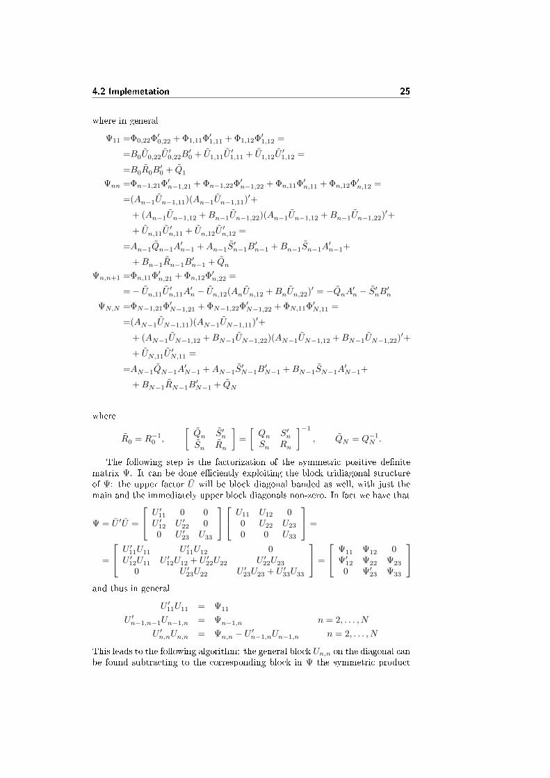
where in general
Ψ11 =Φ0,22Φ′0,22 + Φ1,11Φ′1,11 + Φ1,12Φ′1,12 =
=B0U0,22U′0,22B
′0 + U1,11U
′1,11 + U1,12U
′1,12 =
=B0R0B′0 + Q1
Ψnn =Φn−1,21Φ′n−1,21 + Φn−1,22Φ′n−1,22 + Φn,11Φ′n,11 + Φn,12Φ′n,12 =
=(An−1Un−1,11)(An−1Un−1,11)′+
+ (An−1Un−1,12 +Bn−1Un−1,22)(An−1Un−1,12 +Bn−1Un−1,22)′+
+ Un,11U′n,11 + Un,12U
′n,12 =
=An−1Qn−1A′n−1 +An−1S
′n−1B
′n−1 +Bn−1Sn−1A
′n−1+
+Bn−1Rn−1B′n−1 + Qn
Ψn,n+1 =Φn,11Φ′n,21 + Φn,12Φ′n,22 =
=− Un,11U′n,11A
′n − Un,12(AnUn,12 +BnUn,22)′ = −QnA′n − S′nB′n
ΨN,N =ΦN−1,21Φ′N−1,21 + ΦN−1,22Φ′N−1,22 + ΦN,11Φ′N,11 =
=(AN−1UN−1,11)(AN−1UN−1,11)′+
+ (AN−1UN−1,12 +BN−1UN−1,22)(AN−1UN−1,12 +BN−1UN−1,22)′+
+ UN,11U′N,11 =
=AN−1QN−1A′N−1 +AN−1S
′N−1B
′N−1 +BN−1SN−1A
′N−1+
+BN−1RN−1B′N−1 + QN
where
R0 = R−10 ,
[Qn S′nSn Rn
]=
[Qn S′nSn Rn
]−1
, QN = Q−1N .
The following step is the factorization of the symmetric positive de�nitematrix Ψ. It can be done e�ciently exploiting the block tridiagonal structureof Ψ: the upper factor U will be block diagonal banded as well, with just themain and the immediately upper block diagonals non-zero. In fact we have that
Ψ = U ′U =
U ′11 0 0U ′12 U ′22 00 U ′23 U33
U11 U12 00 U22 U23
0 0 U33
=
=
U ′11U11 U ′11U12 0U ′12U11 U ′12U12 + U ′22U22 U ′22U23
0 U ′23U22 U ′23U23 + U ′33U33
=
Ψ11 Ψ12 0Ψ′12 Ψ22 Ψ23
0 Ψ′23 Ψ33
and thus in general
U ′11U11 = Ψ11
U ′n−1,n−1Un−1,n = Ψn−1,n n = 2, . . . , N
U ′n,nUn,n = Ψn,n − U ′n−1,nUn−1,n n = 2, . . . , N
This leads to the following algorithm: the general block Un,n on the diagonal canbe found subtracting to the corresponding block in Ψ the symmetric product
26 Schur Complement Method
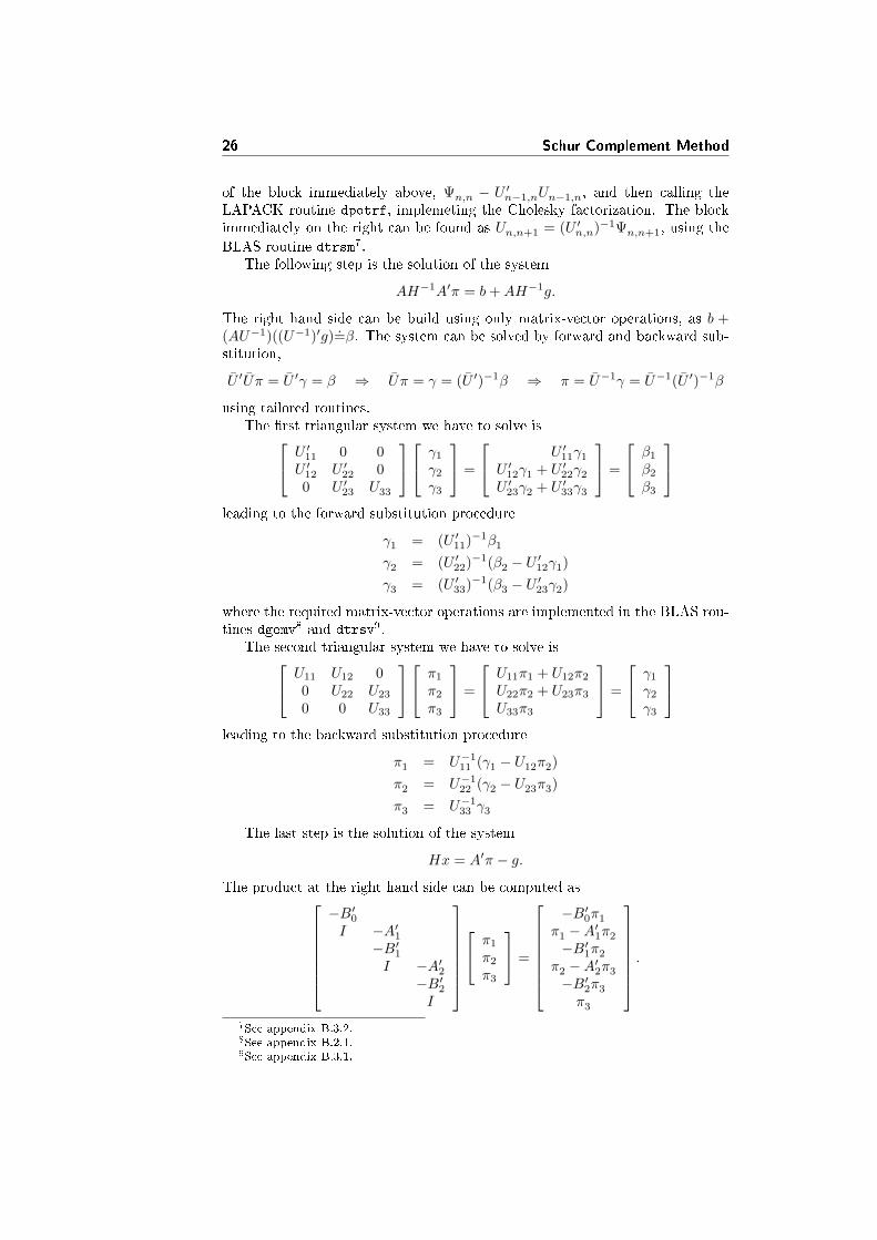
of the block immediately above, Ψn,n − U ′n−1,nUn−1,n, and then calling theLAPACK routine dpotrf, implemeting the Cholesky factorization. The blockimmediately on the right can be found as Un,n+1 = (U ′n,n)−1Ψn,n+1, using the
BLAS routine dtrsm7.The following step is the solution of the system
AH−1A′π = b+AH−1g.
The right hand side can be build using only matrix-vector operations, as b +(AU−1)((U−1)′g)=β. The system can be solved by forward and backward sub-stitution,
U ′Uπ = U ′γ = β ⇒ Uπ = γ = (U ′)−1β ⇒ π = U−1γ = U−1(U ′)−1β
using tailored routines.The �rst triangular system we have to solve is U ′11 0 0
U ′12 U ′22 00 U ′23 U33
γ1
γ2
γ3
=
U ′11γ1
U ′12γ1 + U ′22γ2
U ′23γ2 + U ′33γ3
=
β1
β2
β3
leading to the forward substitution procedure
γ1 = (U ′11)−1β1
γ2 = (U ′22)−1(β2 − U ′12γ1)
γ3 = (U ′33)−1(β3 − U ′23γ2)
where the required matrix-vector operations are implemented in the BLAS rou-tines dgemv8 and dtrsv9.
The second triangular system we have to solve is U11 U12 00 U22 U23
0 0 U33
π1
π2
π3
=
U11π1 + U12π2
U22π2 + U23π3
U33π3
=
γ1
γ2
γ3
leading to the backward substitution procedure
π1 = U−111 (γ1 − U12π2)
π2 = U−122 (γ2 − U23π3)
π3 = U−133 γ3
The last step is the solution of the system
Hx = A′π − g.
The product at the right hand side can be computed as−B′0I −A′1
−B′1I −A′2
−B′2I
π1
π2
π3
=
−B′0π1
π1 −A′1π2
−B′1π2
π2 −A′2π3
−B′2π3
π3
.7See appendix B.3.2.8See appendix B.2.1.9See appendix B.3.1.
4.3 Performance analysis 27
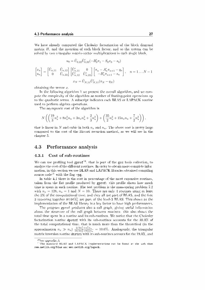
We have already computed the Cholesky factorization of the block diagonalmatrix H, and the inversion of each block factor, and so the system can besolved by two triangular matrix-vector multiplications in each single block,
u0 = U0,22U′0,22(−B′0π1 − S0x0 − s0)[
xnun
]=
[Un,11 Un,12
0 Un,22
] [U ′n,11 0
U ′n,12 U ′n,22
] [πn −A′nπn+1 − qn−B′nπn+1 − sn
], n = 1 . . . N − 1
xN = UN,11U′N,11(πN − qN )
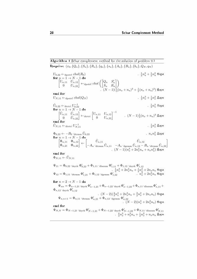
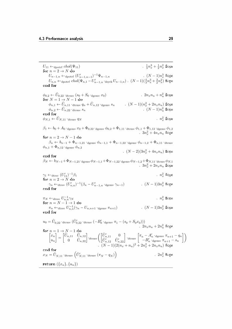
obtaining the vector x.In the following algorithm 1 we present the overall algorithm, and we com-
pute the complexity of the algorithm as number of �oating-point operations upto the quadratic terms. A subscript indicates each BLAS or LAPACK routineused to perform algebra operations.
The asymptotic cost of the algorithm is
N
((19
3n3x + 8n2
xnu + 3nxn2u +
2
3n3u
)+
(35
2n2x + 15nxnu +
7
2n2u
)),
that is linear in N and cubic in both nx and nu. The above cost is pretty largecompared to the cost of the Riccati recursion method, as we will see in thechapter 5.
4.3 Performance analysis
4.3.1 Cost of sub-routines
We can use pro�ling tool gprof10, that is part of the gcc tools collection, toanalyze the cost of the di�erent routines. In order to obtain more complete infor-mation, in this section we use BLAS and LAPACK libraries obtained compilingsource code11 with the �ag -pg.
In table 4.1 there is the cost in percentage of the most expensive routines,taken from the �at pro�le produced by gprof: this pro�le shows how muchtime is spent in each routine. The test problem is the mass-spring problem 7.2with nx = 128, nu = 1 and N = 10. There are only 4 routines using at leastthe 5% of the computational time, and they all are part of BLAS, and the �rst3 (covering together 84.04%) are part of the level-3 BLAS. This shows as theimplementation of the BLAS library is a key factor to have high performances.
The program gprof produces also a call graph, giving useful informationabout the structure of the call graph between routines: this also shows thetotal time spent in a routine and its sub-routines. We notice that the Choleskyfactorization routine dpotrf with its sub-routines accounts for the 39.3% ofthe total computational time, that is much more than the theoretical (in the
approximation nx � nu)2/3n3
x+n2xnu
19/3n2x+8n2
xnu= 10.6%. Analogously, the triangular
matrix inversion routine dtrtri with its sub-routines accouts for the 19.3%, and
10See appendix A11The standard BLAS and LAPACK implementations can be found at the web sites
www.netlib.org/blas and www.netlib.org/lapack.
28 Schur Complement Method
Algorithm 1 Schur complement method for the solution of problem 2.1
Require: (x0, {Qn}, {Sn}, {Rn}, {qn}, {sn}, {An}, {Bn}, {bn}, QN , qN )
U0,22 ←dpotrf chol(R0) . 13n
3u + 1
2n2u �ops
for n = 1→ N − 1 do[Un,11 Un,12
0 Un,22
]←dpotrf chol
([Qn S′nSn Rn
]). (N − 1)( 1
3 (nx + nu)3 + 12 (nx + nu)2) �ops
end for
UN,11 ←dpotrf chol(QN ) . 13n
3x + 1
2n2x �ops
U0,22 ←dtrtri U−10,22 . 1
3n3u �ops
for n = 1→ N − 1 do[Un,11 Un,12
0 Un,22
]←dtrtri
[Un,11 Un,12
0 Un,22
]−1
. (N − 1) 13 (nx + nu)3 �ops
end for
UN,11 ←dtrtri U−1N,11 . 1
3n3x �ops
Φ0,22 ← −B0 ·dtrmm U0,22 . nxn2u �ops
for n = 1→ N − 1 do[Φn,11 Φn,12
Φn,21 Φn,22
]←[
Un,11 Un,12
−An ·dtrmm Un,11 −An ·dgemm Un,12 −Bn ·dtrmm Un,22
]. (N − 1)(n3
x + 2n2xnu + nxn
2u) �ops
end for
ΦN,11 ← UN,11
Ψ11 = Φ0,22 ·dsyrk Φ′0,22 + Φ1,11 ·dlauum Φ′1,11 + Φ1,12 ·dsyrk Φ′1,12
. 13n
3x + 2n2
xnu + 12n
2x + 2nxnu �ops
Ψ12 = Φ1,11 ·dtrmm Φ′1,21 + Φ1,12 ·dgemm Φ′1,22 . n3x + 2n2
xnu �ops
for n = 2→ N − 1 doΨnn = Φn−1,21 ·dsyrk Φ′n−1,21 +Φn−1,22 ·dsyrk Φ′n−1,22 +Φn,11 ·dlauum Φ′n,11 +
Φn,12 ·dsyrk Φ′n,12
. (N − 2)( 43n
3x + 2n2
xnu + 32n
2x + 2nxnu) �ops
Ψn,n+1 = Φn,11 ·dtrmm Φ′n,21 + Φn,12 ·dgemm Φ′n,22
. (N − 2)(n3x + 2n2
xnu) �opsend for
ΨN,N = ΦN−1,21 ·dsyrk Φ′N−1,21 + ΦN−1,22 ·dsyrk Φ′N−1,22 + ΦN,11 ·dlauum Φ′N,11
. 43n
3x + n2
xnu + 12n
2x + nxnu �ops
4.3 Performance analysis 29
U11 ←dpotrf chol(Ψ11) . 13n
3x + 1
2n2x �ops
for n = 2→ N do
Un−1,n ←dpotrf (U ′n−1,n−1)−1Ψn−1,n . (N − 1)n3x �ops
Un,n ←dpotrf chol(Ψn,1−U ′n−1,n ·dsyrk Un−1,n) . (N − 1)( 43n
3x + 3
2n2x) �ops
end for
φ0,2 ← U0,22 ·dtrmv (s0 + S0 ·dgemv x0) . 2nxnu + n2u �ops
for N = 1→ N − 1 doφn,1 ← Un,11 ·dtrmv qn + Un,12 ·dgemv sn . (N − 1)(n2
x + 2nxnu) �ops
φn,2 ← Un,22 ·dtrmv sn . (N − 1)n2u �ops
end for
φN,1 ← UN,11 ·dtrmv qN . n2x �ops
β1 ← b0 +A0 ·dgemv x0 + Φ0,22 ·dgemv φ0,2 + Φ1,11 ·dtrmv φ1,1 + Φ1,12 ·dgemv φ1,2
. 3n2x + 4nxnu �ops
for n = 2→ N − 1 doβn ← bn−1 + Φn−1,21 ·dgemv φn−1,1 + Φn−1,22 ·dgemv φn−1,2 + Φn,11 ·dtrmv
φn,1 + Φn,12 ·dgemv φn,2. (N − 2)(3n2
x + 4nxnu) �opsend for
βN ← bN−1+ΦN−1,21 ·dgemvφN−1,1+ΦN−1,22 ·dgemvφN−1,2+ΦN,11 ·dtrmvφN,1. 3n2
x + 2nxnu �ops
γ1 ←dtrsv (U ′11)−1β1 . n2x �ops
for n = 2→ N do
γn ←dtrsv (U ′n,n)−1(βn − U ′n−1,n ·dgemv γn−1) . (N − 1)3n2x �ops
end for
πN ←dtrsv U−1n,nγN . n2
x �opsfor n = N − 1→ 1 do
πn ←dtrsv U−1n,n(γn − Un,n+1 ·dgemv πn+1) . (N − 1)3n2
x �opsend for
u0 = U0,22 ·dtrmv (U ′0,22 ·dtrmv (−B′0 ·dgemv π1 − (s0 + S0x0))). 2nxnu + 2n2
u �opsfor n = 1→ N − 1 do[
xnun
]=
[Un,11 Un,12
0 Un,22
]·dtrmv
([U ′n,11 0
U ′n,12 U ′n,22
]·dtrmv
[πn −A′n ·dgemv πn+1 − qn−B′n ·dgemv πn+1 − sn
]). (N − 1)(2(nx + nu)2 + 2n2
x + 2nxnu) �opsend for
xN = UN,11 ·dtrmv
(U ′N,11 ·dtrmv (πN − qN )
). 2n2
x �ops
return ({xn}, {un})
30 Schur Complement Method
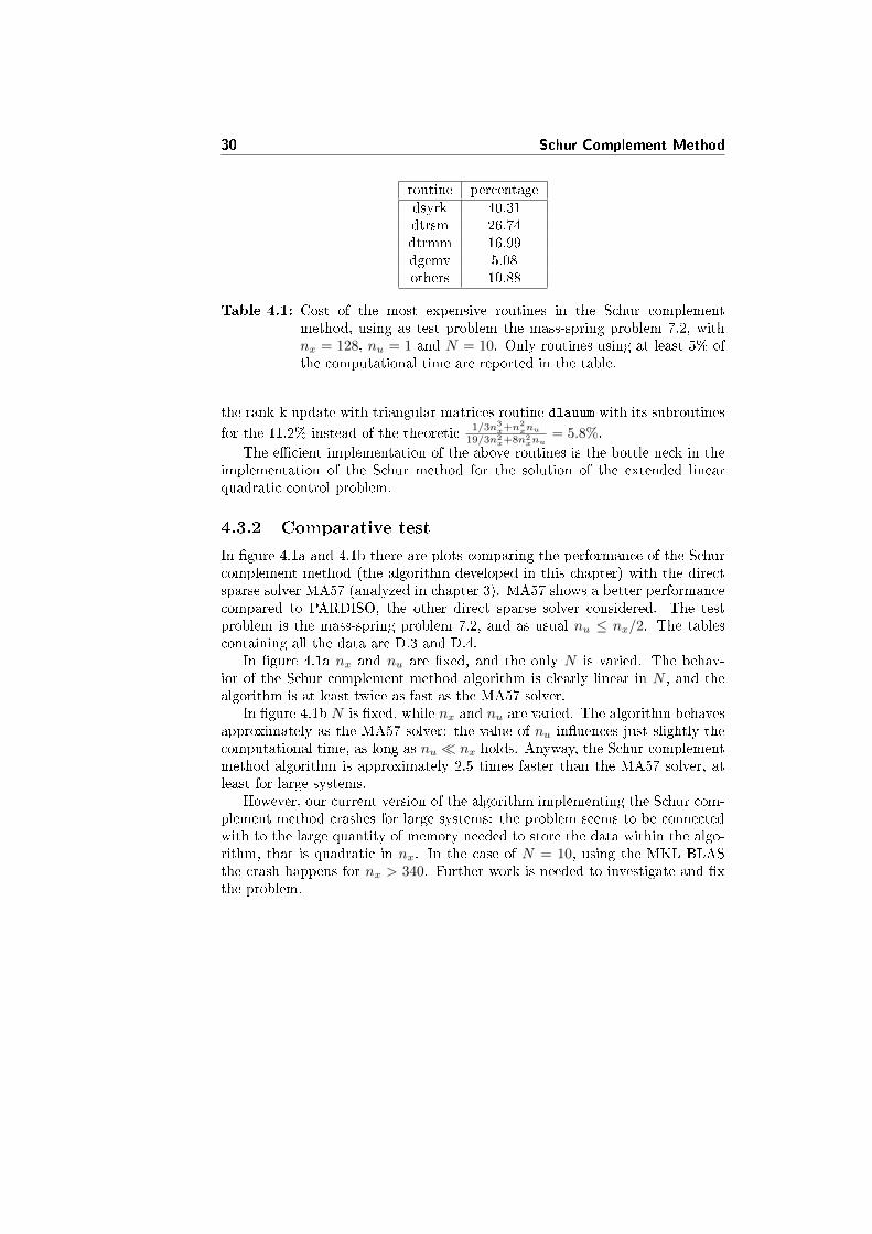
routine percentagedsyrk 40.31dtrsm 26.74dtrmm 16.99dgemv 5.08others 10.88
Table 4.1: Cost of the most expensive routines in the Schur complementmethod, using as test problem the mass-spring problem 7.2, withnx = 128, nu = 1 and N = 10. Only routines using at least 5% ofthe computational time are reported in the table.
the rank-k update with triangular matrices routine dlauum with its subroutines
for the 11.2% instead of the theoretic1/3n3
x+n2xnu
19/3n2x+8n2
xnu= 5.8%.
The e�cient implementation of the above routines is the bottle neck in theimplementation of the Schur method for the solution of the extended linearquadratic control problem.
4.3.2 Comparative test
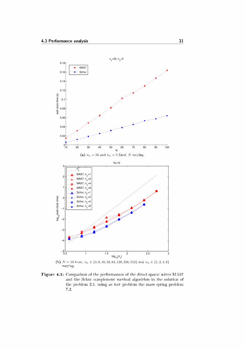
In �gure 4.1a and 4.1b there are plots comparing the performance of the Schurcomplement method (the algorithm developed in this chapter) with the directsparse solver MA57 (analyzed in chapter 3). MA57 shows a better performancecompared to PARDISO, the other direct sparse solver considered. The testproblem is the mass-spring problem 7.2, and as usual nu ≤ nx/2. The tablescontaining all the data are D.3 and D.4.
In �gure 4.1a nx and nu are �xed, and the only N is varied. The behav-ior of the Schur complement method algorithm is clearly linear in N , and thealgorithm is at least twice as fast as the MA57 solver.
In �gure 4.1b N is �xed, while nx and nu are varied. The algorithm behavesapproximately as the MA57 solver: the value of nu in�uences just slightly thecomputational time, as long as nu � nx holds. Anyway, the Schur complementmethod algorithm is approximately 2.5 times faster than the MA57 solver, atleast for large systems.
However, our current version of the algorithm implementing the Schur com-plement method crashes for large systems: the problem seems to be connectedwith to the large quantity of memory needed to store the data within the algo-rithm, that is quadratic in nx. In the case of N = 10, using the MKL BLASthe crash happens for nx > 340. Further work is needed to investigate and �xthe problem.
4.3 Performance analysis 31
10 20 30 40 50 60 70 80 90 1000
0.02
0.04
0.06
0.08
0.1
0.12
0.14
0.16
0.18
nx=50, n
u=5
N
wa
ll clo
ck t
ime
(s)
MA57
Schur
(a) nx = 50 and nu = 5 �xed, N varying.
0.5 1 1.5 2 2.5 3−5
−4
−3
−2
−1
0
1
2
3N=10
log10
(nx)
log
10(w
all
clo
ck tim
e)
n
x
3
MA57, nu=1
MA57, nu=2
MA57, nu=4
MA57, nu=8
Schur, nu=1
Schur, nu=2
Schur, nu=4
Schur, nu=8
(b) N = 10 �xed, nx ∈ {4, 8, 16, 32, 64, 128, 256, 512} and nu ∈ {1, 2, 4, 8}varying.
Figure 4.1: Comparison of the performances of the direct sparse solver MA57and the Schur complement method algorithm in the solution ofthe problem 2.1, using as test problem the mass-spring problem7.2.

32 Schur Complement Method
Chapter 5
Riccati Recursion Method
The Riccati recursion is a well known method for the solution of the standardlinear quadratic control problem 2.2, and the algorithm can be modi�ed for thesolution of problem 2.1. The Riccati recursion methods for the solution of 2.2and 2.1 have asymptotic complexity N(nx + nu)3 (the same as the methodsconsidered in chapters 3 and 4) but in practice they are faster.
5.1 Derivation
There are several ways to derive the Riccati recursion methods for the solutionof problems 2.2 and 2.1. In what follows we consider:
• direct derivation from the cost function expression
• derivation using dynamic programming
• derivation as block factorization procedure for the solution of the KKTsystem.
In this section we derive Riccati recursion methods for the solution of bothproblems 2.2 and 2.1, using the three considered methods.
5.1.1 Derivation from the Cost Function Expression
This derivation technique can be found also in [FM03].
34 Riccati Recursion Method
Standard Linear Quadratic Control Problem
In this chapter we use a equivalent expression for the standard linear quadraticcontrol problem 2.2:
minun,xn+1
φ =
N−1∑n=0
[x′n u′n
] [ Q S′
S R
] [xnun
]+ x′NPxN
s.t. xn+1 = Axn +Bun
(5.1)
The di�erence is the absence of the factor 12 , and the use of P instead of QN .
In this section we show that the solution of the problem 5.1 is the inputsequence un obtained as linear feedback from the state xn with a time variantgain matrix Kn,
un = Knxn
computed using the Riccati recursion.
The matrix R is assumed to be symmetric positive de�nite, and the matrix[Q S′
S R
]to be symmetric positive semi-de�nite.
The �rst step in solving 5.1 is to rewrite the cost function φ in a moreuseful form. We notice that for each sequence of generic squared matrices Pn,n ∈ {0, 1, . . . , N} of size nx × nx, we have
0 = x′0P0x0 − x′0P0x0 + x′1P1x1 − x′1P1x1 + · · ·+ x′NPNxN − x′NPNxN =
= x′0P0x0 − x′NPNxN +
N−1∑n=0
(x′n+1Pn+1xn+1 − x′nPnxn) =
= x′0P0x0 − x′NPNxN +
N−1∑n=0
((Axn +Bun)′Pn+1(Axn +Bun)− x′nPnxn
)=
= x′0P0x0 − x′NPNxN +
N−1∑n=0
([x′n u′n
] [A′B′
]Pn+1
[A B
] [xnun
]− x′nPnxn
)=
= x′0P0x0 − x′NPNxN +
N−1∑n=0
[x′n u′n
] [ A′Pn+1A− Pn A′Pn+1BB′Pn+1A B′Pn+1B
] [xnun
].
Adding this expression to the cost function expression in 5.1, we obtain
φ =x′0P0x0 + x′N (P − PN )xN+
+
N−1∑n=0
[x′n u′n
] [ Q+A′Pn+1A− Pn S′ +A′Pn+1BS +B′Pn+1A R+B′Pn+1B
] [xnun
].
Choosing the ending value of the sequence Pn as PN = P the term x′N (P −PN )xN vanishes. Choosing the remaining element of the sequence such that theexpression of Pn is obtained from Pn+1 as
Pn = Q+A′Pn+1A− (S +B′Pn+1A)′(R+B′Pn+1B)−1(S +B′Pn+1A) (5.2)
5.1 Derivation 35
we have that the quadratic terms of the cost function factorize as
φ = x′0P0x0+
+
N−1∑n=0
[x′n u′n
] [(S′ +A′Pn+1B)(R+B′Pn+1B)−1(S +B′Pn+1A) S′ +A′Pn+1BS +B′Pn+1A R+B′Pn+1B
] [xnun
]=
= x′0P0x0+
+
N−1∑n=0
[x′n u′n
] [(S +B′Pn+1A)′
R+B′Pn+1B
](R+B′Pn+1B)−1 [S +B′Pn+1A R+B′Pn+1B
] [xnun
]=
= x′0P0x0 +
N−1∑n=0
v′n(R+B′Pn+1B)−1vn
wherevn = (S +B′Pn+1A)xn + (R+B′Pn+1B)un.
Equation 5.2 is the well known expression of the Riccati recursion.In the last expression of the cost function the term x′0P0x0 is a constant, and,
since the matrix (R+B′Pn+1B) is positive de�nite (as R is positive de�nite andPn+1 is at least positive semi-de�nite, as shown in 5.1.4), the sum at the secondterm is positive or zero, and the minimum 0 can only be obtained choosingvn = 0 for each n. This implies
un = (R+B′Pn+1B)−1(S +B′Pn+1A)xn=Knxn.
This proves that the optimal input sequence can be written as a linear feedbackfrom the state, with a time variant gain matrix obtained using the Riccatirecursion.
The optimal value of the cost function is
φ∗ = x′0P0x0.
The Riccati recursion method for the solution of problem 2.2 is summarizedin algorithm 1.
Extended Linear Quadratic Control Problem
Also in the case of problem 2.1, in this chapter we use an equivalent expression
minun,xk+1
φ =
N−1∑n=0
1
2
[x′n u′n
] [ Qn S′nSn Rn
] [xnun
]+[q′n s′n
] [ xnun
]+ ρn+
+1
2x′NPxN + p′xN + π
s.t. xn+1 = Anxn +Bnun + bn(5.3)
where we use P , p and π instead of QN , qN and ρN .In this section we show that the solution of problem 5.3 is an input sequence
un obtained as a�ne feedback from the state xn with a time variant gain matrixKn and constant kn,
un = Knxn + kn
36 Riccati Recursion Method
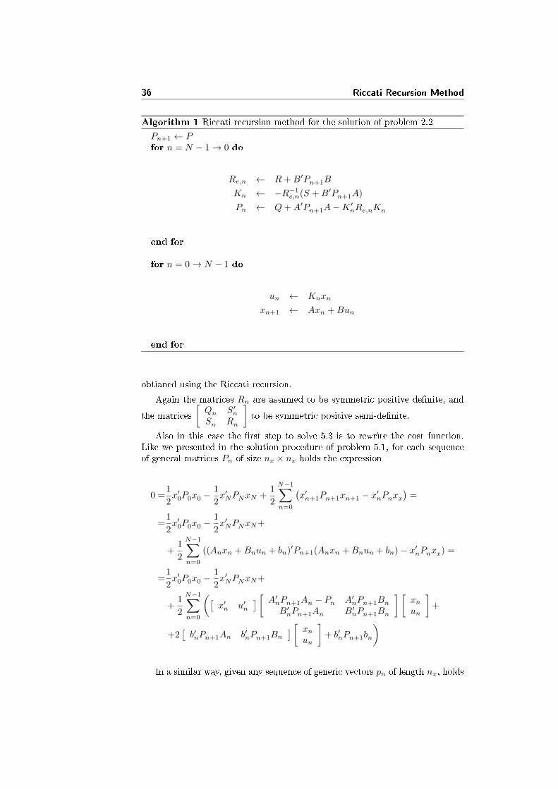
Algorithm 1 Riccati recursion method for the solution of problem 2.2
Pn+1 ← Pfor n = N − 1→ 0 do
Re,n ← R+B′Pn+1B
Kn ← −R−1e,n(S +B′Pn+1A)
Pn ← Q+A′Pn+1A−K ′nRe,nKn
end for
for n = 0→ N − 1 do
un ← Knxn
xn+1 ← Axn +Bun
end for
obtianed using the Riccati recursion.
Again the matrices Rn are assumed to be symmetric positive de�nite, and
the matrices
[Qn S′nSn Rn
]to be symmetric positive semi-de�nite.
Also in this case the �rst step to solve 5.3 is to rewrite the cost function.Like we presented in the solution procedure of problem 5.1, for each sequenceof general matrices Pn of size nx × nx holds the expression
0 =1
2x′0P0x0 −
1
2x′NPNxN +
1
2
N−1∑n=0
(x′n+1Pn+1xn+1 − x′nPnxx
)=
=1
2x′0P0x0 −
1
2x′NPNxN+
+1
2
N−1∑n=0
((Anxn +Bnun + bn)′Pn+1(Anxn +Bnun + bn)− x′nPnxx) =
=1
2x′0P0x0 −
1
2x′NPNxN+
+1
2
N−1∑n=0
([x′n u′n
] [ A′nPn+1An − Pn A′nPn+1BnB′nPn+1An B′nPn+1Bn
] [xnun
]+
+2[b′nPn+1An b′nPn+1Bn
] [ xnun
]+ b′nPn+1bn
)
In a similar way, given any sequence of generic vectors pn of length nx, holds
5.1 Derivation 37
the expression
0 = p′0x0 − p′NxN +
N−1∑n=0
(p′n+1xn+1 − p′nxn
)=
= p′0x0 − p′NxN +
N−1∑n=0
(p′n+1(Anxn +Bnun + bn)− p′nxn
)=
= p′0x0 − p′NxN +
N−1∑n=0
([p′n+1An − p′n p′n+1Bn
] [ xnun
]+ p′n+1bn
)The cost function can thus be rewritten as
φ =1
2x′0P0x0 + p′0x0 +
1
2x′N (P − PN )xx + (p− pN )′xn + π+
+
N−1∑n=0
(1
2
[x′n u′n
] [ Qn +A′nPn+1An − Pn S′n +A′nPn+1BnSn +B′nPn+1An Rn +B′nPn+1Bn
] [xnun
]+
+[q′n + b′nPn+1An + p′n+1An − p′n s′n + b′nPn+1Bn + p′n+1Bn
] [ xnun
]+
+1
2b′nPn+1bn + p′n+1bn + ρn
).
Choosing again the sequence Pn such that PN = P , the term 12x′N (P −
PN )xN is zero. Choosing the remaining elements of the sequence such that theexpression of Pn is obtained from Pn+1 satisfying the Riccati recursion
Pn = Qn+A′nPn+1An−(Sn+B′nPn+1An)′(Rn+B′nPn+1Bn)−1(Sn+B′nPn+1An)
we have that the term quadratic in[x′n u′n
]′in the cost function factorizes as
1
2
[x′n u′n
] [(Sn +B′nPn+1An)′
Rn +B′nPn+1Bn
](Rn+B′nPn+1Bn)−1
[Sn +B′nPn+1An Rn +B′nPn+1Bn
] [xnun
]=
= v′n(Rn +B′nPn+1Bn)−1vn=v′nHnvn
where again
vn = (Sn +B′nPn+1An)xn + (Rn +B′nPn+1Bn)un
and the matrix Hn = (Rn +B′nPn+1Bn)−1 is positive de�nite.The cost function expression becomes
φ =1
2x′0P0x0 + p′0x0 + (p− pN )′xn + π+
+
N−1∑n=0
(1
2v′nHnvn + (b′nPn+1bn + p′n+1bn + ρn)+
+[q′n + b′nPn+1An + p′n+1An − p′n s′n + b′nPn+1Bn + p′n+1Bn
] [ xnun
]).
The aim at this point is to handle also the linear term in[x′n u′n
]′such that
it can be rewritten as a term in vn. Choosing the sequence pn such that pN = p
38 Riccati Recursion Method
the term (p − pN )′xN is zero. Choosing the remaining terms of the sequencesuch that the expression of pn is obtained from pn+1 as
q′n + b′nPn+1An + p′n+1An − p′n =
= (s′n + b′nPn+1Bn + p′n+1Bn)(Rn +B′nPn+1Bn)−1(Sn +B′nPn+1An),
that means
pn = qn +A′n(Pn+1bn + pn+1)−− (Sn +B′nPn+1An)′(Rn +B′nPn+1Bn)−1(sn +B′n(Pn+1bn + pn+1)),
the linear term becomes
(sn+B′n(Pn+1bn+pn+1))(Rn+B′nPn+1Bn)−1 [Sn +B′nPn+1An Rn +B′nPn+1Bn
] [xnun
]=
= (sn +B′n(Pn+1bn + pn+1))(Rn +B′nPn+1Bn)−1vn=g′nvn.
The cost function expression �nally becomes
φ =1
2x′0P0x0+p′0x0+π+
N−1∑n=0
(1
2v′nHnvn + g′nvn + (
1
2b′nPn+1bn + p′n+1bn + ρn)
)and it must be minimized as a function of vn. We notice that the term outsidethe sum is a constant, while for each n the minimum of the positive de�nitequadratic function is obtained setting the gradient with respect to vn to zero:
∇vn(
1
2v′nHnvn + g′nvn + (
1
2b′nPn+1bn + p′n+1bn + ρn)
)= Hnvn + gn = 0.
This means vn = −H−1n gn, and then
(Sn +B′nPn+1An)xn + (Rn +B′nPn+1Bn)un =
= −(Rn +B′nPn+1Bn)(Rn +B′nPn+1Bn)−1(sn +B′n(Pn+1bn + pn+1))
and �nally
un =− (Rn +B′nPn+1Bn)−1(Sn +B′nPn+1An)xn−− (Rn +B′nPn+1Bn)−1(sn +B′n(Pn+1bn + pn+1)) =
=Knxn + kn.
This shows that the optimal input sequence un can be obtained as a time varianta�ne feedback from the state.
The optimal value of the cost function is thus
φ∗ =1
2x′0P0x0 + p′0x0 +
(π +
N−1∑n=0
(−1
2g′nH
−1n gn +
1
2b′nPn+1bn + p′n+1bn + ρn
))
=1
2x′0P0x0 + p′0x0 + π0
5.1 Derivation 39
where
π0 = π +
N−1∑n=0
(1
2b′nPn+1bn + p′n+1bn + ρn−
−1
2(sn +B′n(Pn+1bn + pn+1))′(Rn +B′nPn+1Bn)−1(sn +B′n(Pn+1bn + pn+1))
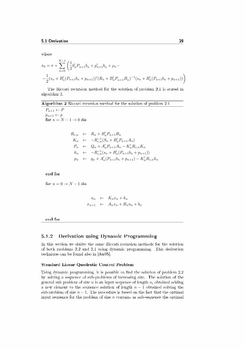
)The Riccati recursion method for the solution of problem 2.1 is stated in
algorithm 2.
Algorithm 2 Riccati recursion method for the solution of problem 2.1
Pn+1 ← Ppn+1 ← pfor n = N − 1→ 0 do
Re,n ← Rn +B′nPn+1Bn
Kn ← −R−1e,n(Sn +B′nPn+1An)
Pn ← Qn +A′nPn+1An −K ′nRe,nKn
kn ← −R−1e,n(sn +B′n(Pn+1bn + pn+1))
pn ← qn +A′n(Pn+1bn + pn+1)−K ′nRe,nkn
end for
for n = 0→ N − 1 do
un ← Knxn + kn
xn+1 ← Anxn +Bnun + bn
end for
5.1.2 Derivation using Dynamic Programming
In this section we derive the same Riccati recursion methods for the solutionof both problems 2.2 and 2.1 using dynamic programming. This derivationtechnique can be found also in [Jør05].
Standard Linear Quadratic Control Problem
Using dynamic programming, it is possible to �nd the solution of problem 2.2by solving a sequence of sub-problems of increasing size. The solution of thegeneral sub-problem of size n is an input sequence of length n, obtained addinga new element to the sequence solution of length n − 1 obtained solving thesub-problem of size n− 1. The procedure is based on the fact that the optimalinput sequence for the problem of size n contains as sub-sequence the optimal
40 Riccati Recursion Method
input sequence for the problem of size n − 1. The solution can thus be buildstarting from the last stage N − 1, solving a trivial problem of size 1. Then, atstage N − 2, the solution is expanded with another term, computed solving atrivial problem of size 1, and so on. In what follows there are the details.
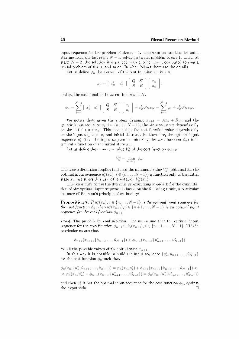
Let us de�ne ϕn the element of the cost function at time n,
ϕn =[x′n u′n
] [ Q S′
S R
] [xnun
],
and φn the cost function between time n and N ,
φn =
N−1∑i=n
[x′i u′i
] [ Q S′
S R
] [xiui
]+ x′NPNxN =
N−1∑i=n
ϕi + x′NPNxN .
We notice that, given the system dynamic xn+1 = Axn + Bun and thegeneric input sequence ui, i ∈ {n, . . . , N − 1}, the state sequence depends onlyon the initial state xn. This means that the cost function value depends onlyon the input sequence ui and initial state xn. Furthermore, the optimal inputsequence u∗i (i.e. the input sequence minimizing the cost function φn) is ingeneral a function of the initial state xn.
Let us de�ne the minimum value V ∗n of the cost function φn as
V ∗n = minui,xi+1
φn.
The above discussion implies that also the minimum value V ∗n (obtained for theoptimal input sequence u∗i (xn), i ∈ {n, . . . , N−1}) is function only of the initialstate xn: we stress this using the notation V
∗n (xn).
The possibility to use the dynamic programming approach for the computa-tion of the optimal input sequence is based on the following result, a particularinstance of Bellman's principle of optimality:
Proposition 7. If u∗i (xn), i ∈ {n, . . . , N − 1} is the optimal input sequence forthe cost function φn, then u
∗i (xn+1), i ∈ {n+ 1, . . . , N − 1} is an optimal input
sequence for the cost function φn+1.
Proof. The proof is by contradiction. Let us assume that the optimal inputsequence for the cost function φn+1 is ui(xn+1), i ∈ {n+ 1, . . . , N − 1}. This inparticular means that
φn+1(xn+1, {un+1, . . . , uN−1}) < φn+1(xn+1, {u∗n+1, . . . , u∗N−1})
for all the possible values of the initial state xn+1.In this way it is possible to build the input sequence {u∗n, un+1, . . . , uN−1}
for the cost function φn such that
φn(xn, {u∗n, un+1, . . . , uN−1}) = ϕn(xn, u∗i ) + φn+1(xn+1, {un+1, . . . , uN−1}) <
< ϕn(xn, u∗n) + φn+1(xn+1, {u∗n+1, . . . , u
∗N−1}) = φn(xn, {u∗n, u∗n+1, . . . , u
∗N−1})
and then u∗i is not the optimal input sequence for the cost function φn, againstthe hypothesis.
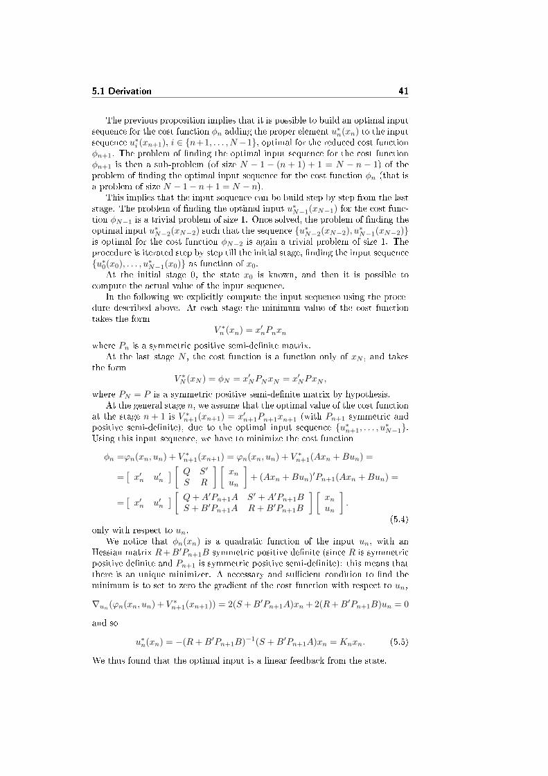
5.1 Derivation 41
The previous proposition implies that it is possible to build an optimal inputsequence for the cost function φn adding the proper element u
∗n(xn) to the input
sequence u∗i (xn+1), i ∈ {n+1, . . . , N−1}, optimal for the reduced cost functionφn+1. The problem of �nding the optimal input sequence for the cost functionφn+1 is then a sub-problem (of size N − 1 − (n + 1) + 1 = N − n − 1) of theproblem of �nding the optimal input sequence for the cost function φn (that isa problem of size N − 1− n+ 1 = N − n).
This implies that the input sequence can be build step by step from the laststage. The problem of �nding the optimal input u∗N−1(xN−1) for the cost func-tion φN−1 is a trivial problem of size 1. Once solved, the problem of �nding theoptimal input u∗N−2(xN−2) such that the sequence {u∗N−2(xN−2), u∗N−1(xN−2)}is optimal for the cost function φN−2 is again a trivial problem of size 1. Theprocedure is iterated step by step till the initial stage, �nding the input sequence{u∗0(x0), . . . , u∗N−1(x0)} as function of x0.
At the initial stage 0, the state x0 is known, and then it is possible tocompute the actual value of the input sequence.
In the following we explicitly compute the input sequence using the proce-dure described above. At each stage the minimum value of the cost functiontakes the form
V ∗n (xn) = x′nPnxn
where Pn is a symmetric positive semi-de�nite matrix.At the last stage N , the cost function is a function only of xN , and takes
the formV ∗N (xN ) = φN = x′NPNxN = x′NPxN ,
where PN = P is a symmetric positive semi-de�nite matrix by hypothesis.At the general stage n, we assume that the optimal value of the cost function
at the stage n + 1 is V ∗n+1(xn+1) = x′n+1Pn+1xn+1 (with Pn+1 symmetric andpositive semi-de�nite), due to the optimal input sequence {u∗n+1, . . . , u
∗N−1}.
Using this input sequence, we have to minimize the cost function
φn =ϕn(xn, un) + V ∗n+1(xn+1) = ϕn(xn, un) + V ∗n+1(Axn +Bun) =
=[x′n u′n
] [ Q S′
S R
] [xnun
]+ (Axn +Bun)′Pn+1(Axn +Bun) =
=[x′n u′n
] [ Q+A′Pn+1A S′ +A′Pn+1BS +B′Pn+1A R+B′Pn+1B
] [xnun
].
(5.4)only with respect to un.
We notice that φn(xn) is a quadratic function of the input un, with anHessian matrix R+B′Pn+1B symmetric positive de�nite (since R is symmetricpositive de�nite and Pn+1 is symmetric positive semi-de�nite): this means thatthere is an unique minimizer. A necessary and su�cient condition to �nd theminimum is to set to zero the gradient of the cost function with respect to un,
∇un(ϕn(xn, un) + V ∗n+1(xn+1)) = 2(S +B′Pn+1A)xn + 2(R+B′Pn+1B)un = 0
and so
u∗n(xn) = −(R+B′Pn+1B)−1(S +B′Pn+1A)xn = Knxn. (5.5)
We thus found that the optimal input is a linear feedback from the state.
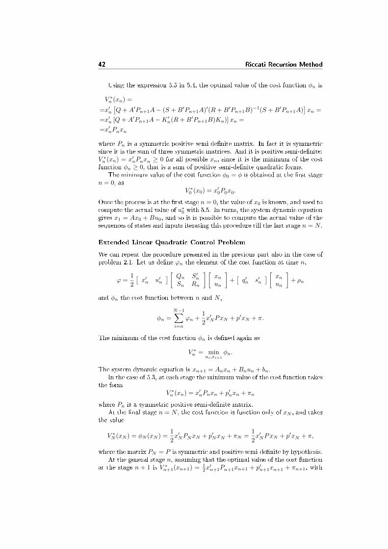
42 Riccati Recursion Method
Using the expression 5.5 in 5.4, the optimal value of the cost function φn is
V ∗n (xn) =
=x′n[Q+A′Pn+1A− (S +B′Pn+1A)′(R+B′Pn+1B)−1(S +B′Pn+1A)
]xn =
=x′n [Q+A′Pn+1A−K ′n(R+B′Pn+1B)Kn)]xn =
=x′nPnxn
where Pn is a symmetric positive semi-de�nite matrix. In fact it is symmetricsince it is the sum of three symmetric matrices. And it is positive semi-de�nite:V ∗n (xn) = x′nPnxn ≥ 0 for all possible xn, since it is the minimum of the costfunction φn ≥ 0, that is a sum of positive semi-de�nite quadratic forms.
The minimum value of the cost function φ0 = φ is obtained at the �rst stagen = 0, as
V ∗0 (x0) = x′0P0x0.
Once the process is at the �rst stage n = 0, the value of x0 is known, and used tocompute the actual value of u∗0 with 5.5. In turns, the system dynamic equationgives x1 = Ax0 + Bu0, and so it is possible to compute the actual value of thesequences of states and inputs iterating this procedure till the last stage n = N .
Extended Linear Quadratic Control Problem
We can repeat the procedure presented in the previous part also in the case ofproblem 2.1. Let us de�ne ϕn the element of the cost function at time n,
ϕ =1
2
[x′n u′n
] [ Qn S′nSn Rn
] [xnun
]+[q′n s′n
] [ xnun
]+ ρn
and φn the cost function between n and N ,
φn =
N−1∑i=n
ϕn +1
2x′NPxN + p′xN + π.
The minimum of the cost function φn is de�ned again as
V ∗n = minui,xi+1
φn.
The system dynamic equation is xn+1 = Anxn +Bnun + bn.In the case of 5.3, at each stage the minimum value of the cost function takes
the formV ∗n (xn) = x′nPnxn + p′nxn + πn
where Pn is a symmetric positive semi-de�nite matrix.At the �nal stage n = N , the cost function is function only of xN , and takes
the value
V ∗N (xN ) = φN (xN ) =1
2x′NPNxN + p′NxN + πN =
1
2x′NP xN + p′xN + π,
where the matrix PN = P is symmetric and positive semi-de�nite by hypothesis.At the general stage n, assuming that the optimal value of the cost function
at the stage n + 1 is V ∗n+1(xn+1) = 12x′n+1Pn+1xn+1 + p′n+1xn+1 + πn+1, with
5.1 Derivation 43
Pn+1 symmetric and positive semi-de�nite, we have to minimize with respectto un the cost function
φn(xn, un) =ϕ(xn, un) + V ∗n+1(xn+1) =
=ϕn(xn, un) + V ∗n+1(Anxn +Bnun + bn) =
=1
2
[x′n u′n
] [Qn S′nSn Rn
] [xnun
]+[q′n s′n
] [xnun
]+ ρn+
+1
2(Anxn +Bnun + bn)′Pn+1(Anxn +Bnun + bn)+
+ p′n+1(Anxn +Bnun + bn) + πn =
=1
2
[x′n u′n
] [Qn +A′nPn+1An S′n +A′nPn+1BnSn +B′nPn+1An Rn +B′nPn+1Bn
] [xnun
]+
+[q′n + (b′nPn+1 + p′n+1)An s′n + (b′nPn+1 + p′n+1)An
] [xnun
]+
+ ρn +1
2b′nPn+1bn + p′n+1bn + πn
We notice that this is a quadratic function of un, with the Hessian matrixRn + B′nPn+1Bn symmetric positive de�nite (since Rn is symmetric positivede�nite and Pn+1 is symmetric positive semi-de�nite): this means that there isan unique minimizer. A necessary and su�cient condition to �nd the minimumis to set to zero the gradient of the cost function with respect to un,
∇un(ϕn(xn, un) + V ∗n+1(xn+1)) =
= (Sn+B′nPn+1Bn)xn+(Rn+B′nPn+1Bn)un+(sn+B′n(Pn+1bn+pn+1)) = 0
and so
u∗n(xn) =− (Rn +B′nPn+1Bn)−1(Sn +B′nPn+1An)xn−− (Rn +B′nPn+1Bn)−1(sn +B′n(Pn+1bn + pn+1))
=Knxn + kn.
We thus found that the optimal input is an a�ne feedback from the state.

44 Riccati Recursion Method
The optimal value of the cost function φn(xn, un) is
V ∗n (xn) = φNn (xn, u∗n(xn)) =
=1
2x′n[Qn +A′nPn+1An+
+(S′n +A′nPn+1Bn)Kn +K ′n(Sn +B′nPn+1An) +K ′n(Rn +B′nPn+1Bn)Kn
]xn+
+ [qn +A′n(Pn+1bn + pn+1) +K ′n(sn +B′n(Pn+1bn + pn+1))+
+(Sn +A′nPn+1Bn)kn + k′n(Rn +B′nPn+1BB)Kn
]+
+
[1
2k′n(Rn +B′nPn+1Bn)kn + (sn +B′n(Pn+1bn + pn+1))′kn + ρ+
+1
2b′nP
′n+1bn + p′n+1bn + πn
]=
=1
2x′n[Qn +A′nPn+1An−
− (Sn +B′nPn+1An)′(Rn +B′nPn+1Bn)−1(Sn +B′nPn+1An)]xn+
+ [qn +A′n(Pn+1bn + pn+1)−
−(Sn +B′nPn+1An)′(Rn +B′nPn+1Bn)−1(sn +B′n(Pn+1bn + pn+1))]′xn+
+
[−1
2(sn +B′n(Pn+1bn + pn+1))′(Rn +B′nPn+1Bn)−1(sn +B′n(Pn+1bn + pn+1))+
+ρn +1
2b′nPn+1bn + p′n+1bn + πn
]=
1
2x′n[Qn +A′nPn+1An −K ′n(Rn +B′nPn+1Bn)Kn
]xn+
+[qn +A′n(Pn+1bn + pn+1)−K ′n(Rn +B′nPn+1Bn)kn
]′xn+
+
[−1
2k′n(Rn +B′nPn+1Bn)kn + ρn +
1
2b′nPn+1bn + p′n+1bn + πn
]=x′nPnxn + p′nxn + πn
where Pn is a symmetric positive semi-de�nite matrix. In fact it is symmetricsince it is the sum of three symmetric matrices. And it is positive semi-de�nite,since its expression is the same (a part form the time variant matrices) as in thestandard linear quadratic control problem case.
The minimum of the cost function φN0 = φ is obtained at the �rst stagen = 0, as
V ∗0 (x0) = x′0P0x0 + p′0x0 + π0.
5.1.3 Derivation from the KKT System
It is possible to derive the Riccati recursion methods directly from the expressionof the KKT system 2.7. The procedure is the same for both problems 2.2 and2.1. This derivation technique can be found also in [RWR98].
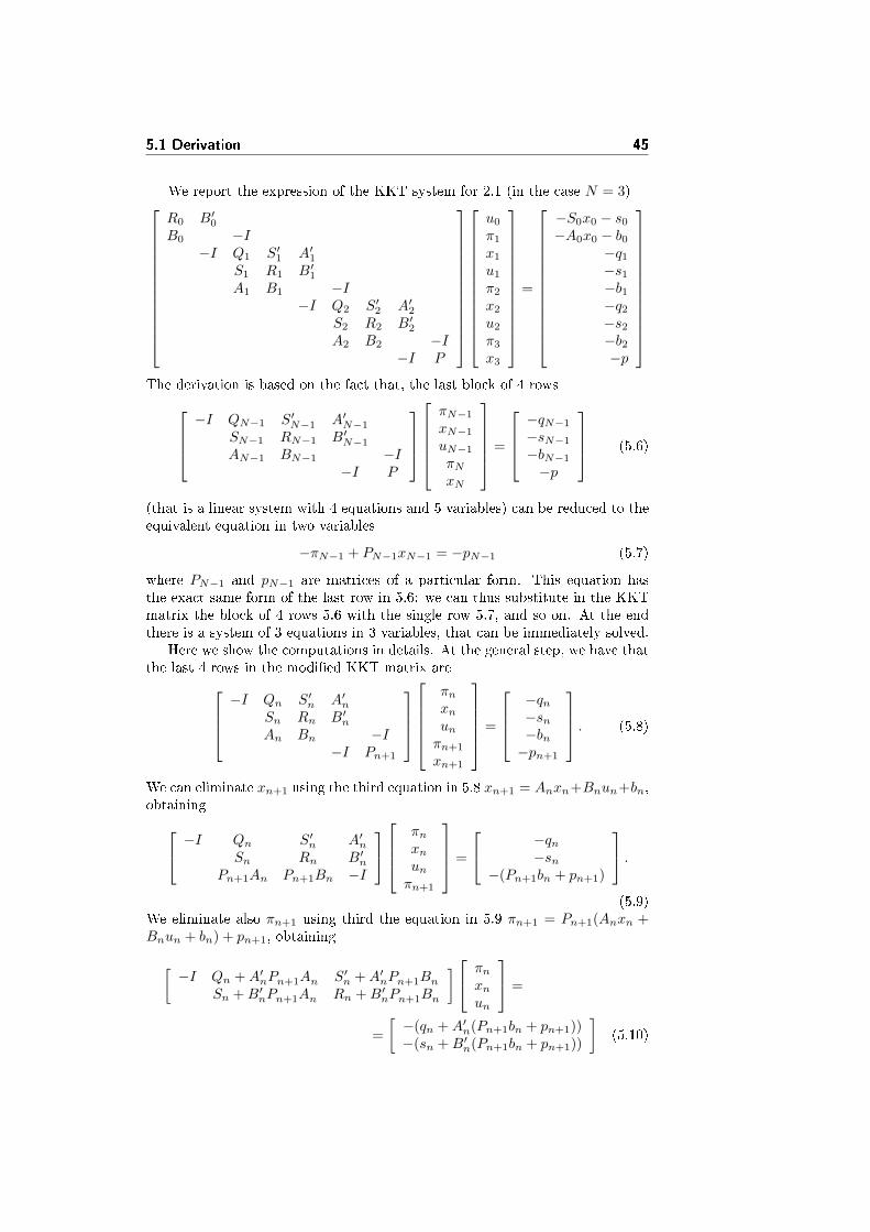
5.1 Derivation 45
We report the expression of the KKT system for 2.1 (in the case N = 3)
R0 B′0B0 −I
−I Q1 S′1 A′1S1 R1 B′1A1 B1 −I
−I Q2 S′2 A′2S2 R2 B′2A2 B2 −I
−I P
u0
π1
x1
u1
π2
x2
u2
π3
x3
=
−S0x0 − s0
−A0x0 − b0−q1
−s1
−b1−q2
−s2
−b2−p
The derivation is based on the fact that, the last block of 4 rows
−I QN−1 S′N−1 A′N−1
SN−1 RN−1 B′N−1
AN−1 BN−1 −I−I P
πN−1
xN−1
uN−1
πNxN
=
−qN−1
−sN−1
−bN−1
−p
(5.6)
(that is a linear system with 4 equations and 5 variables) can be reduced to theequivalent equation in two variables
−πN−1 + PN−1xN−1 = −pN−1 (5.7)
where PN−1 and pN−1 are matrices of a particular form. This equation hasthe exact same form of the last row in 5.6: we can thus substitute in the KKTmatrix the block of 4 rows 5.6 with the single row 5.7, and so on. At the endthere is a system of 3 equations in 3 variables, that can be immediately solved.
Here we show the computations in details. At the general step, we have thatthe last 4 rows in the modi�ed KKT matrix are
−I Qn S′n A′nSn Rn B′nAn Bn −I
−I Pn+1
πnxnunπn+1
xn+1
=
−qn−sn−bn−pn+1
. (5.8)
We can eliminate xn+1 using the third equation in 5.8 xn+1 = Anxn+Bnun+bn,obtaining −I Qn S′n A′n
Sn Rn B′nPn+1An Pn+1Bn −I
πnxnunπn+1
=
−qn−sn
−(Pn+1bn + pn+1)
.(5.9)
We eliminate also πn+1 using third the equation in 5.9 πn+1 = Pn+1(Anxn +Bnun + bn) + pn+1, obtaining[
−I Qn +A′nPn+1An S′n +A′nPn+1BnSn +B′nPn+1An Rn +B′nPn+1Bn
] πnxnun
=
=
[−(qn +A′n(Pn+1bn + pn+1))−(sn +B′n(Pn+1bn + pn+1))
](5.10)
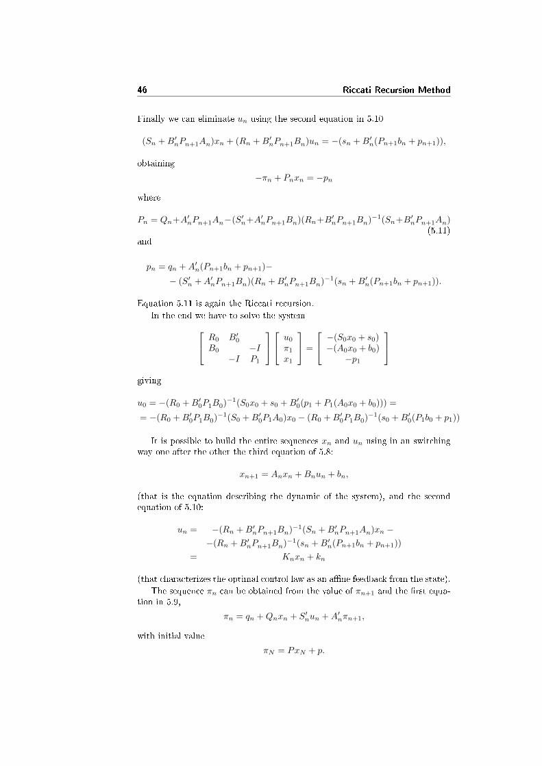
46 Riccati Recursion Method
Finally we can eliminate un using the second equation in 5.10
(Sn +B′nPn+1An)xn + (Rn +B′nPn+1Bn)un = −(sn +B′n(Pn+1bn + pn+1)),
obtaining
−πn + Pnxn = −pn
where
Pn = Qn+A′nPn+1An−(S′n+A′nPn+1Bn)(Rn+B′nPn+1Bn)−1(Sn+B′nPn+1An)(5.11)
and
pn = qn +A′n(Pn+1bn + pn+1)−− (S′n +A′nPn+1Bn)(Rn +B′nPn+1Bn)−1(sn +B′n(Pn+1bn + pn+1)).
Equation 5.11 is again the Riccati recursion.
In the end we have to solve the system R0 B′0B0 −I
−I P1
u0
π1
x1
=
−(S0x0 + s0)−(A0x0 + b0)
−p1
giving
u0 = −(R0 +B′0P1B0)−1(S0x0 + s0 +B′0(p1 + P1(A0x0 + b0))) =
= −(R0 +B′0P1B0)−1(S0 +B′0P1A0)x0 − (R0 +B′0P1B0)−1(s0 +B′0(P1b0 + p1))
It is possible to build the entire sequences xn and un using in an switchingway one after the other the third equation of 5.8:
xn+1 = Anxn +Bnun + bn,
(that is the equation describing the dynamic of the system), and the secondequation of 5.10:
un = −(Rn +B′nPn+1Bn)−1(Sn +B′nPn+1An)xn −−(Rn +B′nPn+1Bn)−1(sn +B′n(Pn+1bn + pn+1))
= Knxn + kn
(that characterizes the optimal control law as an a�ne feedback from the state).
The sequence πn can be obtained from the value of πn+1 and the �rst equa-tion in 5.9,
πn = qn +Qnxn + S′nun +A′nπn+1,
with initial value
πN = PxN + p.
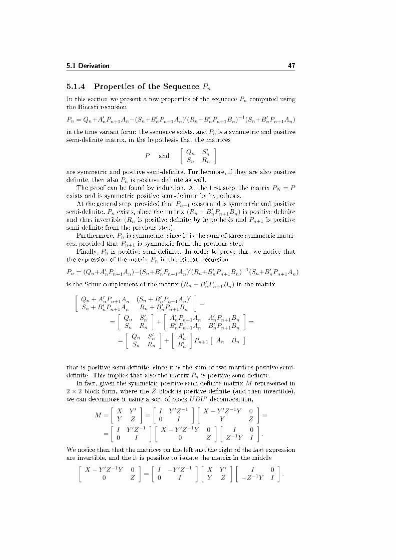
5.1 Derivation 47
5.1.4 Properties of the Sequence Pn
In this section we present a few properties of the sequence Pn computed usingthe Riccati recursion
Pn = Qn+A′nPn+1An−(Sn+B′nPn+1An)′(Rn+B′nPn+1Bn)−1(Sn+B′nPn+1An)
in the time variant form: the sequence exists, and Pn is a symmetric and positivesemi-de�nite matrix, in the hypothesis that the matrices
P and
[Qn S′nSn Rn
]are symmetric and positive semi-de�nite. Furthermore, if they are also positivede�nite, then also Pn is positive de�nite as well.
The proof can be found by induction. At the �rst step, the matrix PN = Pexists and is symmetric positive semi-de�nite by hypothesis.
At the general step, provided that Pn+1 exists and is symmetric and positivesemi-de�nite, Pn exists, since the matrix (Rn +B′nPn+1Bn) is positive de�niteand thus invertible (Rn is positive de�nite by hypothesis and Pn+1 is positivesemi-de�nite from the previous step).
Furthermore, Pn is symmetric, since it is the sum of three symmetric matri-ces, provided that Pn+1 is symmetric from the previous step.
Finally, Pn is positive semi-de�nite. In order to prove this, we notice thatthe expression of the matrix Pn in the Riccati recursion
Pn = (Qn+A′nPn+1An)−(Sn+B′nPn+1An)′(Rn+B′nPn+1Bn)−1(Sn+B′nPn+1An)
is the Schur complement of the matrix (Rn +B′nPn+1Bn) in the matrix[Qn +A′nPn+1An (Sn +B′nPn+1An)′
Sn +B′nPn+1An Rn +B′nPn+1Bn
]=
=
[Qn S′nSn Rn
]+
[A′nPn+1An A′nPn+1BnB′nPn+1An B′nPn+1Bn
]=
=
[Qn S′nSn Rn
]+
[A′nB′n
]Pn+1
[An Bn
]
that is positive semi-de�nite, since it is the sum of two matrices positive semi-de�nite. This implies that also the matrix Pn is positive semi-de�nite.
In fact, given the symmetric positive semi-de�nite matrix M represented in2 × 2 block form, where the Z block is positive de�nite (and then invertible),we can decompose it using a sort of block UDU ′ decomposition,
M =
[X Y ′
Y Z
]=
[I Y ′Z−1
0 I
] [X − Y ′Z−1Y 0
Y Z
]=
=
[I Y ′Z−1
0 I
] [X − Y ′Z−1Y 0
0 Z
] [I 0
Z−1Y I
].
We notice then that the matrices on the left and the right of the last expressionare invertible, and the it is possible to isolate the matrix in the middle[
X − Y ′Z−1Y 00 Z
]=
[I −Y ′Z−1
0 I
] [X Y ′
Y Z
] [I 0
−Z−1Y I
].
48 Riccati Recursion Method
Then, for each vector v of length equal to the size of the X matrix, we havethat
v′(X − Y ′Z−1Y )v =[v′ 0
] [ X − Y ′Z−1Y 00 Z
] [v0
]=
=[v′ 0
] [ I −Y ′Z−1
0 I
] [X Y ′
Y Z
] [I 0
−Z−1Y I
] [v0
]≥ 0
since the M matrix is positive semi-de�nite by hypothesis. This implies thatalso the Schur complement of Z in M , Z − Y ′Z−1Y , is positive semi-de�nite.
Finally, assuming the further hypothesis that the matrices
P and
[Qn S′nSn Rn
]are positive de�nite, it is possible to prove that also Pn is positive de�nite ateach step. The proof is again by induction. At the �rst step it is true thatPN = P is positive de�nite by hypothesis.
At the general step, the expression of the matrix Pn in the Riccati recursion
Pn = (Qn+A′nPn+1An)−(Sn+B′nPn+1An)′(Rn+B′nPn+1Bn)−1(Sn+B′nPn+1An)
is the Schur complement of the matrix (Rn +B′nPn+1Bn) in the matrix[Qn +A′nPn+1An (Sn +B′nPn+1An)′
Sn +B′nPn+1An Rn +B′nPn+1Bn
]=
=
[Qn S′nSn Rn
]+
[A′nPn+1An A′nPn+1BnB′nPn+1An B′nPn+1Bn
]=
=
[Qn S′nSn Rn
]+
[A′nB′n
]Pn+1
[An Bn
]
that this time is positive de�nite, since it is the sum of a matrix positive de�niteand a matrix at least positive semi-de�nite. This implies that also the matrixPn is positive de�nite.
In fact, given a generic symmetric positive de�nite matrix M representedin 2 × 2 block form, we can decompose it using again a sort of block UDU ′
decomposition,
M =
[X Y ′
Y Z
]=
[I Y ′Z−1
0 I
] [X − Y ′Z−1Y 0
0 Z
] [I 0
Z−1Y I
]since the matrix Z is positive de�nite and then invertible.
We can thus write the inverse of the matrix M as
M−1 =
[X Y ′
Y Z
]−1
=
[I 0
−Z−1Y I
] [(X − Y ′Z−1Y )−1 0
0 Z−1
] [I −Y ′Z−1
0 I
]=
=
[(X − Y ′Z−1Y )−1 0
−Z−1Y (X − Y ′Z−1Y )−1 Z−1
] [I −Y ′Z−1
0 I
]=
=
[(X − Y ′Z−1Y )−1 −(X − Y ′Z−1Y )−1Y ′Z−1
−Z−1Y (X − Y ′Z−1Y )−1 Z−1 + Z−1Y (X − Y ′Z−1Y )−1Y ′Z−1
]
5.2 Implementation 49
The matrix M−1 is positive de�nite because it is the inverse of the positivede�nite matrix M . This implies that also the sub-matrix on the top left corner(X − Y ′Z−1Y )−1 is positive de�nite, and its inverse X − Y ′Z−1Y (the Schurcomplement of the matrix Z in M) is positive de�nite too.
5.2 Implementation
In many applications, and in our test problem, nx is (much) larger than nu: weoptimize our implementation for this case. Provided that, the most expensivepart of the Riccati recursion is the computation of the matrix A′PnA. A trivialimplementation of the computation of A′PnA requires roughly 4n3
x �oating-point operations. Anyway it is possible to exploit the special structure of thisexpression to do better: Pn is a symmetric matrix (and in general just positivesemi-de�nite), and it is multiplied on the right by A and on the left by thetranspose A′. Exploiting this we can write an algorithm to compute of theexpression A′PnA with an asymptotic cost of 3n3
x �oating-point operations.Making the further assumption that Pn is positive de�nite (as often in practice),we can write an algorithm with asymptotic cost of 7
3n3x.
We wrote three implementations of the Riccati recursion method:
• the general form of the algorithm, using the general matrix-matrix multi-plication routine for all operations;
• a form exploiting the symmetry of the Pn matrix;
• a form requiring Pn to be symmetric positive de�nite, in the two versionscomputing the upper or lower Cholesky factor.
5.2.1 Genaral form
In this �rst subsection we consider the general form of the algorithm, and useonly the general matrix-matrix multiplication routine dgemm1. The asymptoticcomplexity of the algorithm is N(4n3
x + 6n2xnu + 3nxn
2u + 1
3n3u) �oating-point
operations, worst than the specialized forms of the algorithm.Anyway, this algorithm can show some advantages for small systems, since
the implementation of the routine dgemm is usually more e�cient, and thusfor small matrices it is usually faster than specialized routines like dtrmm2 ordsyrk3.
In the computation of the product A′PnA, that is where the most part ofthe computational time is spent (at least for large systems), we are exploitingthe symmetry of Pn to use the routine dgemm where it is more e�cient: in fact,the best performance is obtained if, in the product, the �rst factor is transposedand the second is not. Since Pn is symmetric Pn = P ′n, and thus we have that
A′PnA = A′P ′nA = A′(P ′nA)
and thus we can use the routine dgemm both time in the more e�cient situation.
1See appendix B.1.1.2See appendix B.1.2.3See appendix B.1.3.
50 Riccati Recursion Method
It is also possible to obtain a further slightly improvement, compared tothe algorithm stated in the previous section, in the computation of the termK ′nRe,nKn in the Pn update formula. In fact the matrix Re,n is symmetricpositive de�nite, and thus it is possible to compute its Cholesky factorization,
Re,n = ΛnΛ′n.
We thus have
K ′nRe,nKn = (Sn +B′nPn+1An)′R−1e,nRe,nR
−1e,n(Sn +B′nPn+1An) =
= (Sn +B′nPn+1An)′R−1e,n(Sn +B′nPn+1An)
= (Sn +B′nPn+1An)′(Λ−1n )′Λ−1
n (Sn +B′nPn+1An)
= (Λ−1n (Sn +B′nPn+1An))′Λ−1
n (Sn +B′nPn+1An) = L′nLn
where Ln is de�ned as
Ln=Λ−1n (Sn +B′nPn+1An)
In this way a multiplication and a linear triangular system solution are avoided,saving 2nxn
2u and nxn
2u �oating-points operations.
It is also possible to obtain similar improvement in the computation of theterm K ′nRe,nkn in the pn update formula, but this time the savings would bein the quadratic terms, and thus in general non in�uential. We have
K ′nRe,nkn = L′nln
where ln is de�ned as
ln=Λ−1n (rn +B′n(Pn+1bn + pn+1)).
Also the computation of the input un is in�uenced, becoming
un = Knxn + kn = (−Λ′n)−1Lnxn + (−Λ′n)−1ln = (−Λ′n)−1(Lnxn + ln),
where again the di�erence in the computational time a�ects a quadratic term.Regarding the space needs, also the sequence of the nu × nu matrices Λi needsto be saved, in addition to the sequences of the nu×nx matrices Li (of the samesize of ki) and the nu × 1 vectors li (of the same size of ki).
In the following algorithm 3 we compute the complexity per iteration up tothe quadratic terms, that is(
4n3x + 6n2
xnu + 3nxnu +1
3n3u
)+
(5n2
x + 7nxn2u +
5
2n2u
)�oating-point operations. We denote with a subscript the name of the usedBLAS or LAPACK routines.
5.2.2 Form exploiting the symmetry of Pn
The algorithm presented in this part exploits the symmetry of the matrices ofthe sequence Pn to obtain an algorithm with asymptotic complexity of N(3n3
x+5n2
xnu + 3nxn2u + 1
3n3u) �oating-point operations.
5.2 Implementation 51
Algorithm 3 Riccati recursion method for the solution of 2.1, general form
Require: (x0, {Qn}, {Sn}, {Rn}, {qn}, {sn}, {An}, {Bn}, {bn}, P, p)Pn+1 ← Ppn+1 ← pfor n = N − 1→ 0 do
Re,n ← Rn +B′n ·dgemm (P ′n+1 ·dgemm Bn) . 2n2xnu + 2nxn
2u − nxnu �ops
Λn ←dpotrf chol(Re,n) . 13n
3u + 1
2x2u �ops
Ln ←dtrsm Λ−1n (Sn + (P ′n+1Bn)′ ·dgemm An) . 2n2
xnu + nxn2u �ops
Pn ← Qn +A′n ·dgemm (P ′n+1 ·dgemm An)− L′n ·dgemm Ln. 4n3
x + 2n2xnu − n2
x �opsln ←dtrsv Λ−1
n (rn +B′n ·dgemv (Pn+1 ·dgemv bn + pn+1)). 2n2
x + 2nxnu + n2u �ops
pn ← qn +A′n ·dgemv (Pn+1bn + pn+1)− L′n ·dgemv ln . 2n2x + 2nxnu �ops
end for
for n = 0→ N − 1 doun ←dtrsv −(Λ′n)−1(Ln ·dgemv xn + ln) . 2nxnu + n2
u �opsxn+1 ← An ·dgemv xn +Bn ·dgemv un + bn . 2n2
x + 2nxnu �opsend for
return ({xn}, {un})
It is possible to write the symmetric matrix Pn as the sum of a lower tri-angular matrix and an upper triangular matrix in such a way that one is thetransposed of the other: Pn = Π + Π′. The cost to obtain the lower triangu-
lar matrix Π is nx(nx−1)2 copies of �oating point numbers and nx �oating-point
divisions. Substituting this expression into A′PnA we have
A′PnA = A′(Π + Π′)A = A′ΠA+A′Π′A = (A′Π′A)′ +A′Π′A
and thus also the matrix A′PnA can be written as the sum of a matrix and itstransposed. The advantage of this procedure is that it is possible to compute Π′ ·A in n3
x �oating-point operations (instead of roughly 2n3x) using the specialized
BLAS routine dtrmm. The choice of Π′ instead of Π has the advantage of exploitthe used column-major order of data in memory.
The following multiplication A′ · (ΠA) has no structure, and so requires2n3
x �oating-point operations; again the fact that the �rst factor is transposed
exploits the data order in memory. The �nal sum requires nx(nx+1)2 �oating-
point sums and nx(nx−1)2 copies of �oating-point numbers.
The asymptotic complexity in the computation of the term A′PnA is thusof 3n3
x instead of 4n3x �oating-point operations.
All the remaining parts of the algorithm are as in the previous version, withthe only exception of the use of the specialized routine dsyrk (approximatelyrequiring the half of the �oating-point operations compared to dgemm) in thecomputation of the product L′nLn.
In the following algorithm 4 we compute the complexity per iteration up tothe quadratic terms, that is(
3n3x + 5n2
xnu + 3nxn2u +
1
3n3u
)+
(7n2
x + 8nxnu +5
2n2u
)
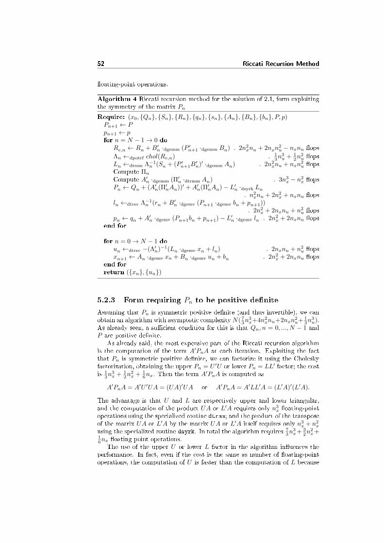
52 Riccati Recursion Method
�oating-point operations.
Algorithm 4 Riccati recursion method for the solution of 2.1, form exploitingthe symmetry of the matrix Pn
Require: (x0, {Qn}, {Sn}, {Rn}, {qn}, {sn}, {An}, {Bn}, {bn}, P, p)Pn+1 ← Ppn+1 ← pfor n = N − 1→ 0 do
Re,n ← Rn +B′n ·dgemm (P ′n+1 ·dgemm Bn) . 2n2xnn + 2nxn
2u − nxnu �ops
Λn ←dpotrf chol(Re,n) . 13n
3u + 1
2n2u �ops
Ln ←dtrsm Λ−1n (Sn + (P ′n+1B
′n)′ ·dgemm An) . 2n2
xnu + nxn2u �ops
Compute Πn
Compute A′n ·dgemm (Π′n ·dtrmm An) . 3n3x − n2
x �opsPn ← Qn + (A′n(Π′nAn))′ +A′n(Π′nAn)− L′n ·dsyrk Ln
. n2xnu + 2n2
x + nxnu �opsln ←dtrsv Λ−1
n (rn +B′n ·dgemv (Pn+1 ·dgemv bn + pn+1)). 2n2
x + 2nxnu + n2u �ops
pn ← qn +A′n ·dgemv (Pn+1bn + pn+1)− L′n ·dgemv ln . 2n2x + 2nxnu �ops
end for
for n = 0→ N − 1 doun ←dtrsv −(Λ′n)−1(Ln ·dgemv xn + ln) . 2nxnu + n2
u �opsxn+1 ← An ·dgemv xn +Bn ·dgemv un + bn . 2n2
x + 2nxnu �opsend for
return ({xn}, {un})
5.2.3 Form requiring Pn to be positive de�nite
Assuming that Pn is symmetric positive de�nite (and thus invertible), we canobtain an algorithm with asymptotic complexity N( 7
3n3x+4n2
xnu+2nxn2u+ 1
3n3u).
As already seen, a su�cient condition for this is that Qn, n = 0, ..., N − 1 andP are positive de�nite.
As already said, the most expensive part of the Riccati recursion algorithmis the computation of the term A′PnA at each iteration. Exploiting the factthat Pn is symmetric positive de�nite, we can factorize it using the Choleskyfactorization, obtaining the upper Pn = U ′U or lower Pn = LL′ factor; the costis 1
3n3x + 1
2n2x + 1
6nx. Then the term A′PnA is computed as
A′PnA = A′U ′UA = (UA)′UA or A′PnA = A′LL′A = (L′A)′(L′A).
The advantage is that U and L are respectively upper and lower triangular,and the computation of the product UA or L′A requires only n3
x �oating-pointoperations using the specialized routine dtrmm; and the product of the transposeof the matrix UA or L′A by the matrix UA or L′A itself requires only n3
x + n2x
using the specialized routine dsyrk. In total the algorithm requires 73n
3x+ 3
2n2x+
16nx �oating point operations.
The use of the upper U or lower L factor in the algorithm in�uences theperformance. In fact, even if the cost is the same as number of �oating-pointoperations, the computation of U is faster than the computation of L because
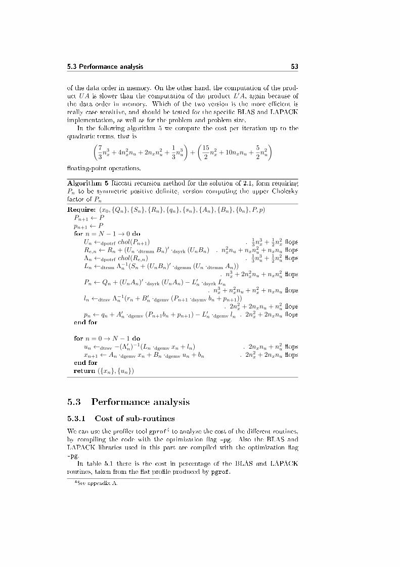
5.3 Performance analysis 53
of the data order in memory. On the other hand, the computation of the prod-uct UA is slower than the computation of the product L′A, again because ofthe data order in memory. Which of the two version is the more e�cient isreally case sensitive, and should be tested for the speci�c BLAS and LAPACKimplementation, as well as for the problem and problem size.
In the following algorithm 5 we compute the cost per iteration up to thequadratic terms, that is(
7
3n3x + 4n2
xnu + 2nxn2u +
1
3n3u
)+
(15
2n2x + 10nxnu +
5
2n2u
)�oating-point operations.
Algorithm 5 Riccati recursion method for the solution of 2.1, form requiringPn to be symmetric positive de�nite, version computing the upper Choleskyfactor of Pn
Require: (x0, {Qn}, {Sn}, {Rn}, {qn}, {sn}, {An}, {Bn}, {bn}, P, p)Pn+1 ← Ppn+1 ← Pfor n = N − 1→ 0 do
Un ←dpotrf chol(Pn+1) . 13n
3x + 1
2n2x �ops
Re,n ← Rn + (Un ·dtrmm Bn)′ ·dsyrk (UnBn) . n2xnu + nxn
2u + nxnu �ops
Λn ←dpotrf chol(Re,n) . 13n
3u + 1
2n2u �ops
Ln ←dtrsm Λ−1n (Sn + (UnBn)′ ·dgemm (Un ·dtrmm An))
. n3x + 2n2
xnu + nxn2u �ops
Pn ← Qn + (UnAn)′ ·dsyrk (UnAn)− L′n ·dsyrk Ln. n3
x + n2xnu + n2
x + nxnu �opsln ←dtrsv Λ−1
n (rn +B′n ·dgemv (Pn+1 ·dsymv bn + pn+1)). 2n2
x + 2nxnu + n2u �ops
pn ← qn +A′n ·dgemv (Pn+1bn + pn+1)− L′n ·dgemv ln . 2n2x + 2nxnu �ops
end for
for n = 0→ N − 1 doun ←dtrsv −(Λ′n)−1(Ln ·dgemv xn + ln) . 2nxnu + n2
u �opsxn+1 ← An ·dgemv xn +Bn ·dgemv un + bn . 2n2
x + 2nxnu �opsend for
return ({xn}, {un})
5.3 Performance analysis
5.3.1 Cost of sub-routines
We can use the pro�ler tool gprof4 to analyze the cost of the di�erent routines,by compiling the code with the optimization �ag -pg. Also the BLAS andLAPACK libraries used in this part are compiled with the optimization �ag-pg.
In table 5.1 there is the cost in percentage of the BLAS and LAPACKroutines, taken from the �at pro�le produced by pgrof.
4See appendix A.
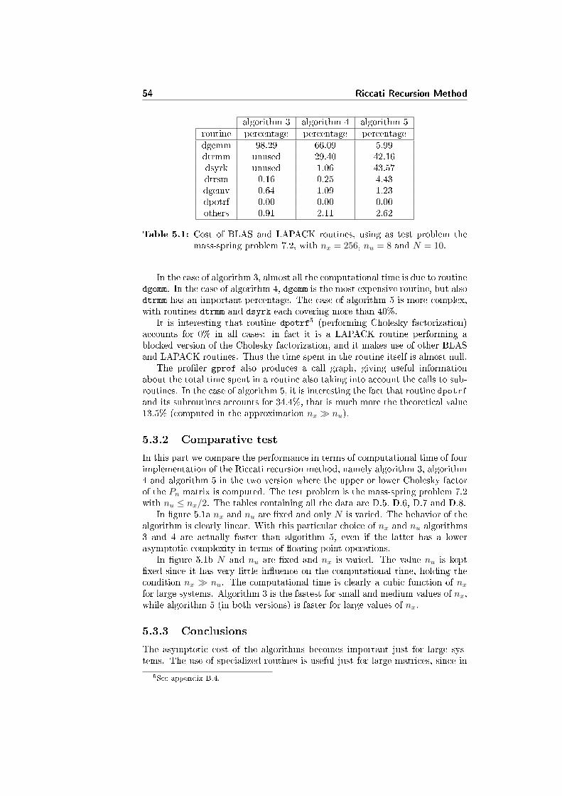
54 Riccati Recursion Method
algorithm 3 algorithm 4 algorithm 5routine percentage percentage percentagedgemm 98.29 66.09 5.99dtrmm unused 29.40 42.16dsyrk unused 1.06 43.57dtrsm 0.16 0.25 4.43dgemv 0.64 1.09 1.23dpotrf 0.00 0.00 0.00others 0.91 2.11 2.62
Table 5.1: Cost of BLAS and LAPACK routines, using as test problem themass-spring problem 7.2, with nx = 256, nu = 8 and N = 10.
In the case of algorithm 3, almost all the computational time is due to routinedgemm. In the case of algorithm 4, dgemm is the most expensive routine, but alsodtrmm has an important percentage. The case of algorithm 5 is more complex,with routines dtrmm and dsyrk each covering more than 40%.
It is interesting that routine dpotrf5 (performing Cholesky factorization)accounts for 0% in all cases: in fact it is a LAPACK routine performing ablocked version of the Cholesky factorization, and it makes use of other BLASand LAPACK routines. Thus the time spent in the routine itself is almost null.
The pro�ler gprof also produces a call graph, giving useful informationabout the total time spent in a routine also taking into account the calls to sub-routines. In the case of algorithm 5, it is interesting the fact that routine dpotrfand its subroutines accounts for 34.4%, that is much more the theoretical value13.5% (computed in the approximation nx � nu).
5.3.2 Comparative test
In this part we compare the performance in terms of computational time of fourimplementation of the Riccati recursion method, namely algorithm 3, algorithm4 and algorithm 5 in the two version where the upper or lower Cholesky factorof the Pn matrix is computed. The test problem is the mass-spring problem 7.2with nu ≤ nx/2. The tables containing all the data are D.5, D.6, D.7 and D.8.
In �gure 5.1a nx and nu are �xed and only N is varied. The behavior of thealgorithm is clearly linear. With this particular choice of nx and nu algorithms3 and 4 are actually faster than algorithm 5, even if the latter has a lowerasymptotic complexity in terms of �oating-point operations.
In �gure 5.1b N and nu are �xed and nx is varied. The value nu is kept�xed since it has very little in�uence on the computational time, holding thecondition nx � nu. The computational time is clearly a cubic function of nxfor large systems. Algorithm 3 is the fastest for small and medium values of nx,while algorithm 5 (in both versions) is faster for large values of nx.
5.3.3 Conclusions
The asymptotic cost of the algorithms becomes important just for large sys-tems. The use of specialized routines is useful just for large matrices, since in
5See appendix B.4.
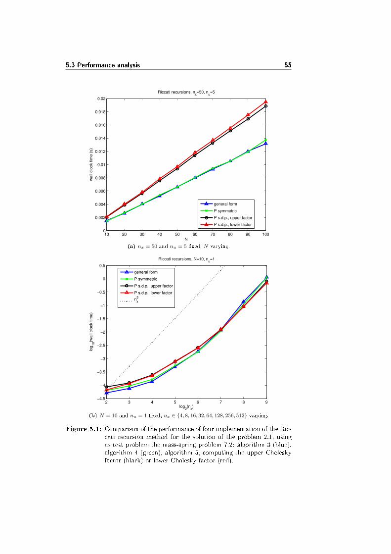
5.3 Performance analysis 55
10 20 30 40 50 60 70 80 90 1000
0.002
0.004
0.006
0.008
0.01
0.012
0.014
0.016
0.018
0.02
Riccati recursions, nx=50, n
u=5
N
wall
clo
ck tim
e (
s)
general form
P symmetric
P s.d.p., upper factor
P s.d.p., lower factor
(a) nx = 50 and nu = 5 �xed, N varying.
2 3 4 5 6 7 8 9−4.5
−4
−3.5
−3
−2.5
−2
−1.5
−1
−0.5
0
0.5
Riccati recursions, N=10, nu=1
log2(n
x)
log
10(w
all
clo
ck tim
e)
general form
P symmetric
P s.d.p., upper factor
P s.d.p., lower factor
nx
3
(b) N = 10 and nu = 1 �xed, nx ∈ {4, 8, 16, 32, 64, 128, 256, 512} varying.
Figure 5.1: Comparison of the performance of four implementation of the Ric-cati recursion method for the solution of the problem 2.1, usingas test problem the mass-spring problem 7.2: algorithm 3 (blue),algorithm 4 (green), algorithm 5, computing the upper Choleskyfactor (black) or lower Cholesky factor (red).
56 Riccati Recursion Method
general they are slower for small ones. For small systems, the best solution isthus the general form algorithm 3, using only routine dgemm for matrix-matrixmultiplication.
For large systems, the best solution is algorithm 5 requiring Pn to be sym-metric positive de�nite. Anyway, the performance is lower than the theoreticalone due to the poor performance of the LAPACK routine dpotrf compared tothe others BLAS routines. For small systems, this problem can partially besolved with the use of a recursive algorithm (as ric2 presented in the appendixC) and e�cient implementation in assembly of the base cases.
Chapter 6
Condensing Methods
Another approach for the solution of problem 2.1 consists in rewrite the problemfrom the form of a large sparse equality constrained quadratic program to a smalldense system of linear equations, whose matrix is positive de�nite and has sizeNnu ×Nnu. The solution of this system can be computed using the Choleskyfactorization in time proportional to (Nnu)3, plus the time needed to build thesystem.
6.1 Derivation
We consider two di�erent methods, and show how they lead to the same systemof linear equaitons:
• the �rst one is the null space method for the solution of a generic equalityconstrained quadratic program
• the second one is the state elimination method: it explicitly uses thesystem dynamic equation to eliminate the states from the problem formu-lation and rewrite it as a small dense unconstrained quadratic program,whose solution is found setting its gradient to zero.
6.1.1 Null space method
This section is divided into two parts: in the �rst part we derive the null spacemethod in the case of a generic equality constrained quadratic program. In thesecond one we use the method in the special case of problem 2.1. The use ofnull space method for the solution of the general equality constrained quadraticprogram can be found in [NW06].
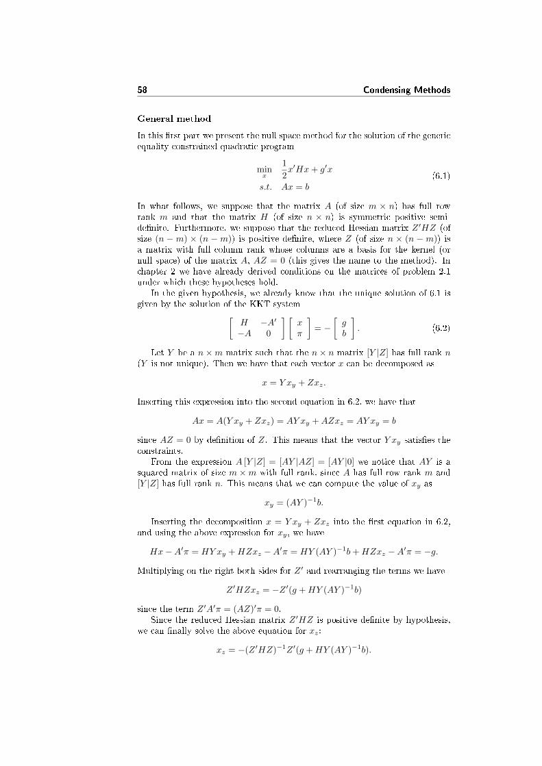
58 Condensing Methods
General method
In this �rst part we present the null space method for the solution of the genericequality constrained quadratic program
minx
1
2x′Hx+ g′x
s.t. Ax = b(6.1)
In what follows, we suppose that the matrix A (of size m × n) has full rowrank m and that the matrix H (of size n × n) is symmetric positive semi-de�nite. Furthermore, we suppose that the reduced Hessian matrix Z ′HZ (ofsize (n − m) × (n − m)) is positive de�nite, where Z (of size n × (n − m)) isa matrix with full column rank whose columns are a basis for the kernel (ornull space) of the matrix A, AZ = 0 (this gives the name to the method). Inchapter 2 we have already derived conditions on the matrices of problem 2.1under which these hypotheses hold.
In the given hypothesis, we already know that the unique solution of 6.1 isgiven by the solution of the KKT system[
H −A′−A 0
] [xπ
]= −
[gb
]. (6.2)
Let Y be a n×m matrix such that the n× n matrix [Y |Z] has full rank n(Y is not unique). Then we have that each vector x can be decomposed as
x = Y xy + Zxz.
Inserting this expression into the second equation in 6.2, we have that
Ax = A(Y xy + Zxz) = AY xy +AZxz = AY xy = b
since AZ = 0 by de�nition of Z. This means that the vector Y xy satis�es theconstraints.
From the expression A [Y |Z] = [AY |AZ] = [AY |0] we notice that AY is asquared matrix of size m ×m with full rank, since A has full row rank m and[Y |Z] has full rank n. This means that we can compute the value of xy as
xy = (AY )−1b.
Inserting the decomposition x = Y xy + Zxz into the �rst equation in 6.2,and using the above expression for xy, we have
Hx−A′π = HY xy +HZxz −A′π = HY (AY )−1b+HZxz −A′π = −g.
Multiplying on the right both sides for Z ′ and rearranging the terms we have
Z ′HZxz = −Z ′(g +HY (AY )−1b)
since the term Z ′A′π = (AZ)′π = 0.Since the reduced Hessian matrix Z ′HZ is positive de�nite by hypothesis,
we can �nally solve the above equation for xz:
xz = −(Z ′HZ)−1Z ′(g +HY (AY )−1b).
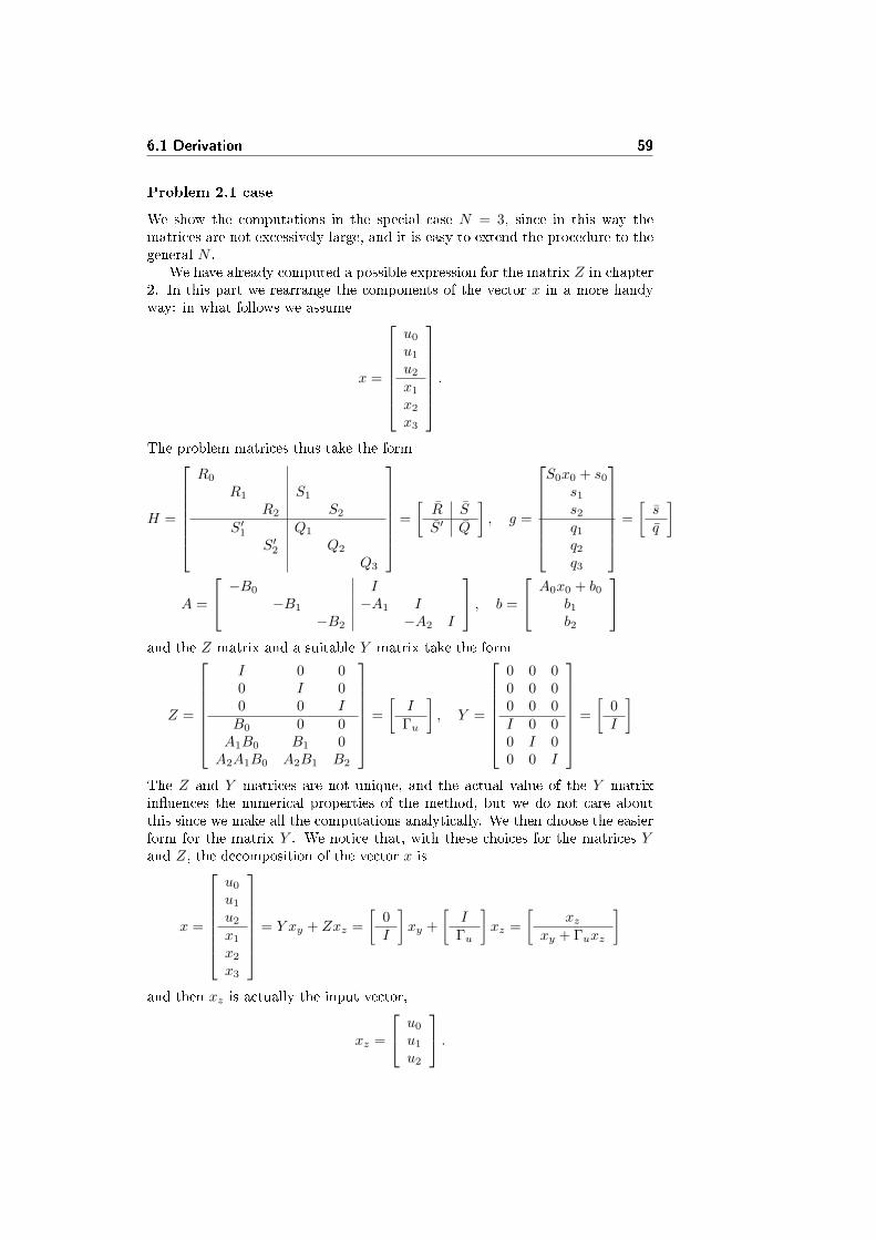
6.1 Derivation 59
Problem 2.1 case
We show the computations in the special case N = 3, since in this way thematrices are not excessively large, and it is easy to extend the procedure to thegeneral N .
We have already computed a possible expression for the matrix Z in chapter2. In this part we rearrange the components of the vector x in a more handyway: in what follows we assume
x =
u0
u1
u2
x1
x2
x3
.
The problem matrices thus take the form
H =
R0
R1 S1
R2 S2
S′1 Q1
S′2 Q2
Q3
=
[R SS′ Q
], g =
S0x0 + s0
s1
s2
q1
q2
q3
=
[sq
]
A =
−B0 I−B1 −A1 I
−B2 −A2 I
, b =
A0x0 + b0b1b2
and the Z matrix and a suitable Y matrix take the form
Z =
I 0 00 I 00 0 IB0 0 0A1B0 B1 0A2A1B0 A2B1 B2
=
[I
Γu
], Y =
0 0 00 0 00 0 0I 0 00 I 00 0 I
=
[0I
]
The Z and Y matrices are not unique, and the actual value of the Y matrixin�uences the numerical properties of the method, but we do not care aboutthis since we make all the computations analytically. We then choose the easierform for the matrix Y . We notice that, with these choices for the matrices Yand Z, the decomposition of the vector x is
x =
u0
u1
u2
x1
x2
x3
= Y xy + Zxz =
[0I
]xy +
[I
Γu
]xz =
[xz
xy + Γuxz
]
and then xz is actually the input vector,
xz =
u0
u1
u2
.
60 Condensing Methods
With these de�nitions, we have that the vector xy is
xy = (AY )−1b =
I 0 0−A1 I 0
0 −A2 I
−1 A0x0 + b0b1b2
=Γbb =
=
I 0 0A1 I 0A2A1 A2 I
A0x0 + b0b1b2
=
A0x0 + b0A1(A0x0 + b0) + b1
A2(A1(A0x0 + b0) + b1) + b2
and �nally xz is
xz = −(Z ′HZ)−1(Z ′(g +HY xy)
)=− H−1g
where
H = Z ′HZ =[I Γ′u
] [ R SS′ R
] [I
Γu
]= R+ Γ′uS
′ + SΓu + Γ′uQΓu =
=
R0 0 00 R1 00 0 R2
+
0 B′0S′1 B′0A
′1S′2
0 0 B′1S′2
0 0 0
+
0 0 0S1B0 0 0S2A1B0 S2B1 0
+
+
B′0Q1B0 +B′0A
′1Q2A1B0 +B′0A
′1A′2Q3A2A1B0
S1B0 +B′1Q2A1B0 +B′1A′2Q3A2A1B0
S2A1B0 +B′2Q3A2A1B0
. . .
. . .
. . .
B′0S′1 +B′0A
′1Q2B1 +B′0A
′1A′2Q3A2B1
R1 +B′1Q2B1 +B′1A′2Q3A2B1
S2B1 +B′2Q3A2B1
B′0A′1A′2Q3B2
B′1S′2 +B′1A
′2Q3B2
R2 +B′2Q3B2
=
R0 +B′0Q1B0 +B′0A′1Q2A1B0 +B′0A
′1A′2Q3A2A1B0
B′1Q2A1B0 +B′1A′2Q3A2A1B0
B′2Q3A2A1B0
. . .
. . .
. . .
B′0S′1 +B′0A
′1Q2B1 +B′0A
′1A′2Q3A2B1
B′1Q2B1 +B′1A′2Q3A2B1
B′2Q3A2B1
B′0A′1S′2 +B′0A
′1A′2Q3B2
B′1A′2Q3B2
B′2Q3B2
and
g = Z ′(g +HY xy) =[I Γ′u
]([ sq
]+
[SQ
]Γbb
)=
=[I Γ′u
] [ s+ SΓbbq + QΓbb
]= s+ SΓbb+ Γ′u(q + QΓbb) =
=
s0 + S0x0 +B′0(q1 +Q1(A0x0 + b0)) +B′0A′1(q2 +Q2(A1(A2x0 + b0) + b1)+
+B′0A′1A′2(q3 +Q3(A2(A1(A0x0 + b0) + b1) + b2))
s1 + S1(A0x0 + b0) +B′1(q2 +Q2(A1(A0x0 + b0) + b1))+
+B′1A′2(q3 +Q3(A2(A1(A0x0 + b0) + b1) + b2))
s2 + S2(A1(A0x0 + b0) + b1)) +B′2(q3 +Q3(A2(A1(A0x0 + b0) + b1) + b2))
6.1 Derivation 61
6.1.2 State elimination
A di�erent approach, leading to the same system of linear equations, is the stateelimination method: exploiting the fact that it is possible to write the futurestates xk, k ∈ {1, . . . , N} as function of the initial state x0 and the (unknown)inputs uk, k ∈ {0, 1, . . . , N − 1}, it is possible to eliminate the states from theformulation of problem 2.1, dropping the direct dependence on the state vector.
The method consist of two phases: the preprocessing phase, rewriting theproblem in the form of an unconstrained quadratic program, with a cost de�nitepositive cost function in the only inputs uk; and the solution phase, where theunconstrained quadratic program is solved by setting its gradient to zero.
We derive the method directly in the case of problem 2.1, for a general valueof N .
Let us de�ne the unknown input vector as
u =
u0
u1
...nN−1
that is a vector of size Nnu × 1.
Our purpose is to rewrite the cost function φ as a quadratic function of theonly u, given the initial state vector x0 of size nx × 1, and the system dynamicequation
xk+1 = Akxk +Bkuk + bk. (6.3)
The cost function can be rewritten as
φ =
N−1∑n=0
(1
2x′nQnxn + x′nS
′nun +
1
2u′nRnun + q′nxn + s′nun + ρn
)+
+1
2x′NQNxN + q′NxN + ρN =
=1
2
N∑n=1
x′nQnxn +
N−1∑n=1
x′nS′nun +
1
2
N−1∑n=0
u′nRnun +
N∑n=1
q′nxn+
+
(x′0S
′0u0 +
N−1∑n=0
s′nun
)+
(1
2x′0Q0x0 + q′0x0 +
N∑n=0
ρn
)=
=1
2x′Qx+
1
2x′S′u+
1
2u′Sx+
1
2u′RU + q′x+ s′u+ ρ,
where we de�ne the scalar ρ = 12x′0Q0x0 + q′0x0 +
∑Nn=0 ρn and the matrices
x =
x1
x2
...xN
, Q =
Q1 0 . . . 0
0 Q2. . .
......
. . .. . . 0
0 . . . 0 QN
, S =
0 . . . . . . 0
S1. . .
.... . .
. . ....
0 . . . SN−1 0
R =
R0 0. . .
0 RN−1
, q =
q1
...qN
, s =
s0 + S0x0
...sN−1
62 Condensing Methods
of size: x is Nnx × 1, Q is Nnx ×Nnx, S is Nnu ×Nnx, R is Nnu ×Nnu, qis Nnx × 1 and r is Nnu × 1.
Using equation 6.3, the state vector can be written as
x = Φxx0 + Γuu+ Γbb (6.4)
where
Φx =
A0
A1A0
AN−1 . . . A1A0
, Γu =
B0 0 . . . 0
A1B0 B1. . .
......
.... . . 0
AN−1 . . . A1B0 AN−1 . . . A2B1 . . . BN−1
Γb =
I 0 . . . 0
A1 I. . .
......
.... . . 0
AN−1 . . . A1 AN−1 . . . A2 . . . I
, b =
b0...
bN−1
Substituting 6.4 into the cost function expression, we obtain the formulation
as a function of the only u
φ = φ(u) =1
2u′Hu+ g′u+ ρ
where
H = Γ′uQΓu + Γ′uS′ + SΓu + R
g = Γ′uQ(Φxx0 + Γbb) + S(Φxx0 + Γbb) + Γ′uq + s
ρ =1
2(Φxx0 + Γbb)
′Q(Φxx0 + Γbb) + q′(Φxx0 + Γbb) + ρ
The matrix H is Nnu ×Nnu, the vector g is Nnu × 1 and ρ is a scalar.We notice that the H matrix is exactly the same as in the null space method,
and that the matrices Φx and Γb are used only in the expression Φxx0 + Γbb.Then de�ning
Φxx0 + Γbb = Γbb
where
b =
A0x0 + b0
b1...
bN−1
we �nd again for g the expression
g = Γ′uQΓbb+ SΓbb+ Γ′uq + s
that is the exactly same as in the null space method.The H matrix is positive de�nite, since it coincides with the reduced Hessian
Z ′HZ matrix of the null space method, that is positive de�nite by hypothesis.
6.2 Implementation 63
The H matrix is then invertible, and so the minimum of the cost function isunique, and can be found setting to zero the gradient of the cost function withrespect to u:
∇φ(u) = Hu+ g = 0 ⇒ u∗ = −H−1g.
The value of ρ does not in�uence the minimizer u∗ but just the value of theminimum of the cost function: since we are only interested in the value of theminimizer and not on the value of the minimum, we avoid the computation ofρ.
6.2 Implementation
In the case of the condensing methods, the implementation plays a key role inthe performance of the algorithm: in fact, the matrices de�ned in the previoussection have a lot of structure, and exploiting this fact it is possible to writealgorithms using much less space and time.
As we have already seen, the algorithm consist in two parts: a �rst part(preprocessing phase), where the H matrix and the g vector are build; anda second part (solution phase) where the system of linear equations is solved.The H matrix is symmetric positive de�nite by hypothesis, and so we can solvethe system of linear equations using the Cholesky factorization. The H matrixhas size Nnu, and then the cost for the factorization of the matrix is roughly13 (Nnu)3, cubic in both the horizon length N and the input number nu.
In the previous chapters we saw algorithms for the solution of 2.1 in timelinear in N and cubic in both nx and nu: then the �eld of application of thecondensing methods is necessary the case of problems with small values of thehorizon length N and the number of inputs nu.
In the condensing phase, it is usually possible to use two di�erent approachesin the construction of matrices, leading to di�erent complexities: an approachproduces algorithm with higher complexity in N and lower in nx, while on theopposite the other approach produces algorithms with lower complexity in Nand higher in nx. Since the solution phase is already cubic in N , we choose the�rst approach, in the hope to obtain an algorithm with good performances inthe case of large value of nx. This is true, since following this approach it ispossible to obtain an algorithm quadratic in nx, while the algorithms presentedin the previous chapters are cubic in nx.
We notice that the Q, S and R matrices are mainly zeros, and can becomevery large (especially Q, of size Nnx × Nnx): the only function of these zerosis to keep the sub-matrices Qk, Sk, Rk in the correct position during matrixmultiplications. Then it is possible to avoid the construction of these matrices,and instead explicitly perform the correct matrix multiplications using the sub-matrices, at the cost of a larger number of calls to the matrix multiplicationroutine dgemm1. The number of calls to this routine is linear in N .
The largest matrix is Γb, of size Nnx ×Nnx; it is used only in the productΓbb, that is a vector of size Nnx × 1. In the case N = 3 this product is written
1See appendix B.1.1.
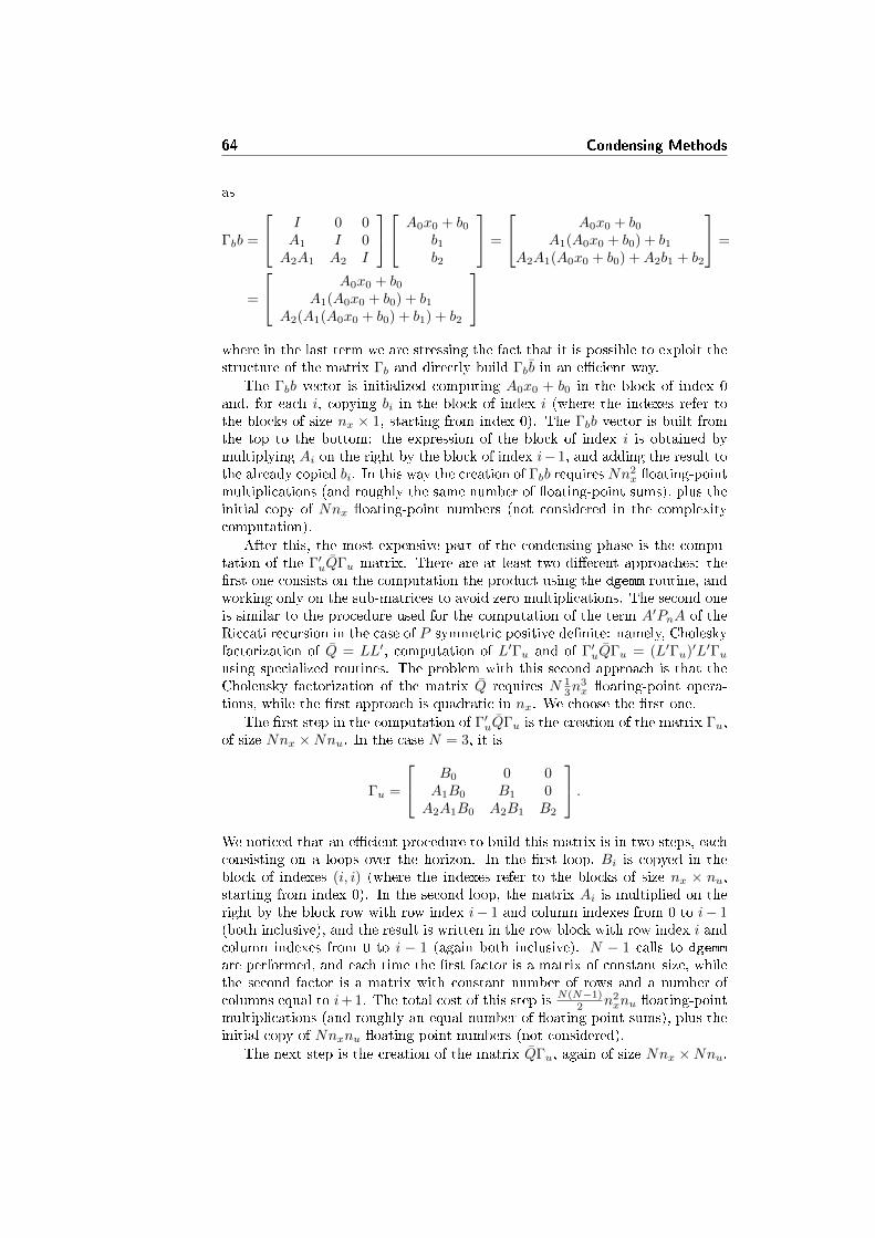
64 Condensing Methods
as
Γbb =
I 0 0A1 I 0A2A1 A2 I
A0x0 + b0b1b2
=
A0x0 + b0A1(A0x0 + b0) + b1
A2A1(A0x0 + b0) +A2b1 + b2
=
=
A0x0 + b0A1(A0x0 + b0) + b1
A2(A1(A0x0 + b0) + b1) + b2
where in the last term we are stressing the fact that it is possible to exploit thestructure of the matrix Γb and directly build Γbb in an e�cient way.
The Γbb vector is initialized computing A0x0 + b0 in the block of index 0and, for each i, copying bi in the block of index i (where the indexes refer tothe blocks of size nx × 1, starting from index 0). The Γbb vector is built fromthe top to the bottom: the expression of the block of index i is obtained bymultiplying Ai on the right by the block of index i− 1, and adding the result tothe already copied bi. In this way the creation of Γbb requires Nn
2x �oating-point
multiplications (and roughly the same number of �oating-point sums), plus theinitial copy of Nnx �oating-point numbers (not considered in the complexitycomputation).
After this, the most expensive part of the condensing phase is the compu-tation of the Γ′uQΓu matrix. There are at least two di�erent approaches: the�rst one consists on the computation the product using the dgemm routine, andworking only on the sub-matrices to avoid zero multiplications. The second oneis similar to the procedure used for the computation of the term A′PnA of theRiccati recursion in the case of P symmetric positive de�nite: namely, Choleskyfactorization of Q = LL′, computation of L′Γu and of Γ′uQΓu = (L′Γu)′L′Γuusing specialized routines. The problem with this second approach is that theCholensky factorization of the matrix Q requires N 1
3n3x �oating-point opera-
tions, while the �rst approach is quadratic in nx. We choose the �rst one.
The �rst step in the computation of Γ′uQΓu is the creation of the matrix Γu,of size Nnx ×Nnu. In the case N = 3, it is
Γu =
B0 0 0A1B0 B1 0A2A1B0 A2B1 B2
.We noticed that an e�cient procedure to build this matrix is in two steps, eachconsisting on a loops over the horizon. In the �rst loop, Bi is copyed in theblock of indexes (i, i) (where the indexes refer to the blocks of size nx × nu,starting from index 0). In the second loop, the matrix Ai is multiplied on theright by the block row with row index i− 1 and column indexes from 0 to i− 1(both inclusive), and the result is written in the row block with row index i andcolumn indexes from 0 to i − 1 (again both inclusive). N − 1 calls to dgemm
are performed, and each time the �rst factor is a matrix of constant size, whilethe second factor is a matrix with constant number of rows and a number ofcolumns equal to i+ 1. The total cost of this step is N(N−1)
2 n2xnu �oating-point
multiplications (and roughly an equal number of �oating-point sums), plus theinitial copy of Nnxnu �oating-point numbers (not considered).
The next step is the creation of the matrix QΓu, again of size Nnx ×Nnu.
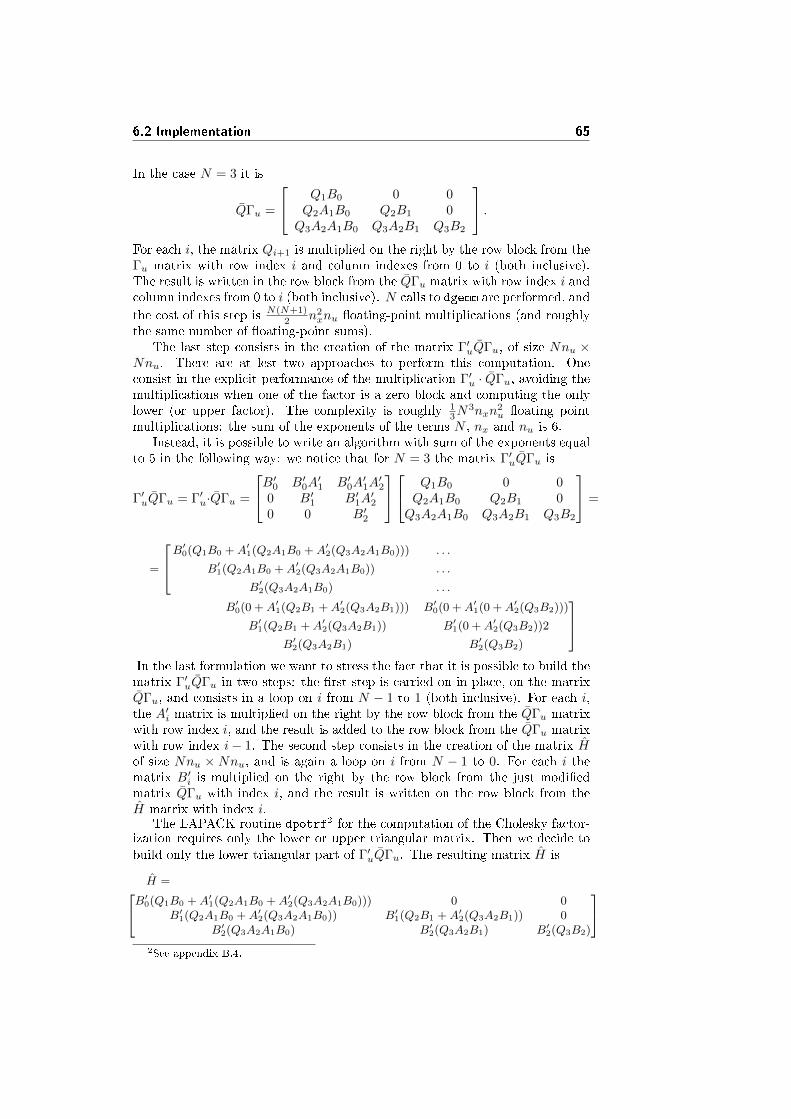
6.2 Implementation 65
In the case N = 3 it is
QΓu =
Q1B0 0 0Q2A1B0 Q2B1 0Q3A2A1B0 Q3A2B1 Q3B2
.For each i, the matrix Qi+1 is multiplied on the right by the row block from theΓu matrix with row index i and column indexes from 0 to i (both inclusive).The result is written in the row block from the QΓu matrix with row index i andcolumn indexes from 0 to i (both inclusive). N calls to dgemm are performed, and
the cost of this step is N(N+1)2 n2
xnu �oating-point multiplications (and roughlythe same number of �oating-point sums).
The last step consists in the creation of the matrix Γ′uQΓu, of size Nnu ×Nnu. There are at lest two approaches to perform this computation. Oneconsist in the explicit performance of the multiplication Γ′u · QΓu, avoiding themultiplications when one of the factor is a zero block and computing the onlylower (or upper factor). The complexity is roughly 1
3N3nxn
2u �oating point
multiplications: the sum of the exponents of the terms N , nx and nu is 6.Instead, it is possible to write an algorithm with sum of the exponents equal
to 5 in the following way: we notice that for N = 3 the matrix Γ′uQΓu is
Γ′uQΓu = Γ′u·QΓu =
B′0 B′0A′1 B′0A
′1A′2
0 B′1 B′1A′2
0 0 B′2
Q1B0 0 0Q2A1B0 Q2B1 0Q3A2A1B0 Q3A2B1 Q3B2
=
=
B′0(Q1B0 +A′1(Q2A1B0 +A′2(Q3A2A1B0)))
B′1(Q2A1B0 +A′2(Q3A2A1B0))
B′2(Q3A2A1B0)
. . .
. . .
. . .
B′0(0 +A′1(Q2B1 +A′2(Q3A2B1)))
B′1(Q2B1 +A′2(Q3A2B1))
B′2(Q3A2B1)
B′0(0 +A′1(0 +A′2(Q3B2)))
B′1(0 +A′2(Q3B2))2
B′2(Q3B2)
In the last formulation we want to stress the fact that it is possible to build thematrix Γ′uQΓu in two steps: the �rst step is carried on in place, on the matrixQΓu, and consists in a loop on i from N − 1 to 1 (both inclusive). For each i,the A′i matrix is multiplied on the right by the row block from the QΓu matrixwith row index i, and the result is added to the row block from the QΓu matrixwith row index i− 1. The second step consists in the creation of the matrix Hof size Nnu × Nnu, and is again a loop on i from N − 1 to 0. For each i thematrix B′i is multiplied on the right by the row block from the just modi�edmatrix QΓu with index i, and the result is written on the row block from theH matrix with index i.
The LAPACK routine dpotrf2 for the computation of the Cholesky factor-ization requires only the lower or upper triangular matrix. Then we decide tobuild only the lower triangular part of Γ′uQΓu. The resulting matrix H is
H =B′0(Q1B0 +A′1(Q2A1B0 +A′2(Q3A2A1B0))) 0 0B′1(Q2A1B0 +A′2(Q3A2A1B0)) B′1(Q2B1 +A′2(Q3A2B1)) 0
B′2(Q3A2A1B0) B′2(Q3A2B1) B′2(Q3B2)
2See appendix B.4.
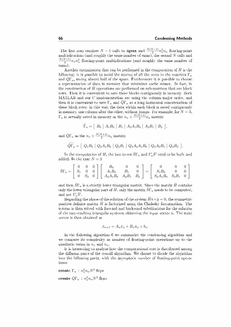
66 Condensing Methods
The �rst step requires N − 1 calls to dgemm and N(N−1)2 n2
xnu �oating-pointmultiplications (and roughly the same number of sums), the second N calls andN(N+1)
2 nxn2u �oating-point multiplications (and roughly the same number of
sums).Another optimization that can be performed in the computation of H is the
following: it is possible to avoid the storing of all the zeros in the matrices Γuand QΓu, saving almost half of the space. Furthermore it is possible to choosea representation of data in memory that minimizes cache misses. In fact, inthe construction of H operations are performed on sub-matrices that are blockrows. Then it is convenient to save these blocks contiguously in memory. BothMATLAB and our C implementation are using the column-major order, andthen it is convenient to save Γu and QΓu as a long horizontal concatenation ofthese block rows: in this way, the data within each block is saved contiguouslyin memory, one column after the other, without jumps. For example, for N = 3,
Γu is actually saved in memory as the nx × N(N+1)2 nu matrix:
Γu =[B0 A1B0 B1 A2A1B0 A2B1 B2
],
and QΓu as the nx × N(N+1)2 nu matrix:
˜QΓu =[Q1B0 Q2A1B0 Q2B1 Q3A2A1B0 Q3A2B1 Q3B2
].
In the computation of H, the two terms SΓu and Γ′uS′ need to be built and
added. In the case N = 3
SΓu =
0 0 0S1 0 00 S2 0
B0 0 0A1B0 B1 0A2A1B0 A2B1 B2
=
0 0 0S1B0 0 0S2A1B0 S2B1 0
and then SΓu is a strictly lower triangular matrix. Since the matrix H containsonly the lower triangular part of H, only the matrix SΓu needs to be computed,and not Γ′uS
′.Regarding the phase of the solution of the system Hu+ g = 0, the symmetric
positive de�nite matrix H is factorized using the Cholesky factorization. Thesystem is then solved with forward and backward substitutions for the solutionof the two resulting triangular systems, obtaining the input vector u. The statevector is then obtained as
xn+1 = Anxn +Bnun + bn.
In the following algorithm 6 we summarize the condensing algorithm andwe compute its complexity as number of �oating-point operations up to thequadratic terms in nx and nu.
It is interesting to analyze how the computational cost is distributed amongthe di�erent parts of the overall algorithm. We choose to divide the algorithminto the following parts, with the asymptotic number of �oating-point opera-tions:
create Γu : n2xnuN
2 �ops
create QΓu : n2xnuN
2 �ops
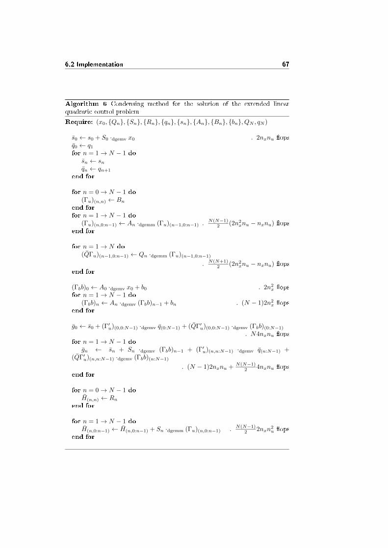
6.2 Implementation 67
Algorithm 6 Condensing method for the solution of the extended linearquadratic control problem
Require: (x0, {Qn}, {Sn}, {Rn}, {qn}, {sn}, {An}, {Bn}, {bn}, QN , qN )
s0 ← s0 + S0 ·dgemv x0 . 2nxnu �opsq0 ← q1
for n = 1→ N − 1 dosn ← snqn ← qn+1
end for
for n = 0→ N − 1 do(Γu)(n,n) ← Bn
end for
for n = 1→ N − 1 do(Γu)(n,0:n−1) ← An ·dgemm (Γu)(n−1,0:n−1) .
N(N−1)2 (2n2
xnu − nxnu) �opsend for
for n = 1→ N do
(QΓu)(n−1,0:n−1) ← Qn ·dgemm (Γu)(n−1,0:n−1)
. N(N+1)2 (2n2
xnu − nxnu) �opsend for
(Γbb)0 ← A0 ·dgemv x0 + b0 . 2n2x �ops
for n = 1→ N − 1 do(Γbb)n ← An ·dgemv (Γbb)n−1 + bn . (N − 1)2n2
x �opsend for
g0 ← s0 + (Γ′u)(0,0:N−1) ·dgemv q(0:N−1) + (QΓ′u)(0,0:N−1) ·dgemv (Γbb)(0:N−1)
. N4nxnu �opsfor n = 1→ N − 1 do
gn ← sn + Sn ·dgemv (Γbb)n−1 + (Γ′u)(n,n:N−1) ·dgemv q(n:N−1) +(QΓ′u)(n,n:N−1) ·dgemv (Γbb)(n:N−1)
. (N − 1)2nxnu + N(N−1)2 4nxnu �ops
end for
for n = 0→ N − 1 doH(n,n) ← Rn
end for
for n = 1→ N − 1 doH(n,0:n−1) ← H(n,0:n−1) + Sn ·dgemm (Γu)(n,0:n−1) . N(N−1)
2 2nxn2u �ops
end for
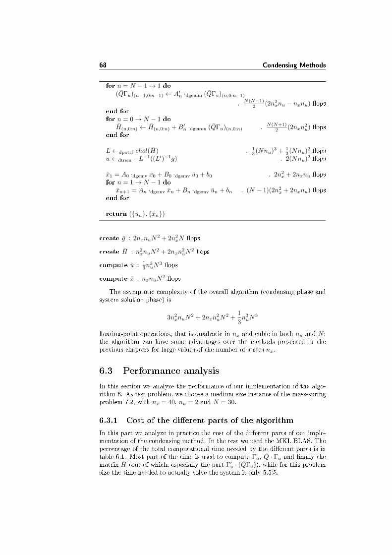
68 Condensing Methods
for n = N − 1→ 1 do(QΓu)(n−1,0:n−1) ← A′n ·dgemm (QΓu)(n,0:n−1)
. N(N−1)2 (2n2
xnu − nxnu) �opsend for
for n = 0→ N − 1 doH(n,0:n) ← H(n,0:n) +B′n ·dgemm (QΓu)(n,0:n) . N(N+1)
2 (2nxn2u) �ops
end for
L←dpotrf chol(H) . 13 (Nnu)3 + 1
2 (Nnu)2 �opsu←dtrsm −L−1((L′)−1g) . 2(Nnu)2 �ops
x1 = A0 ·dgemv x0 +B0 ·dgemv u0 + b0 . 2n2x + 2nxnu �ops
for n = 1→ N − 1 doxn+1 = An ·dgemv xn +Bn ·dgemv un + bn . (N − 1)(2n2
x + 2nxnu) �opsend for
return ({un}, {xn})
create g : 2nxnuN2 + 2n2
xN �ops
create H : n2xnuN
2 + 2nxn2uN
2 �ops
compute u : 13n
3uN
3 �ops
compute x : nxnuN2 �ops
The asymptotic complexity of the overall algorithm (condensing phase andsystem solution phase) is
3n2xnuN
2 + 2nxn2uN
2 +1
3n3uN
3
�oating-point operations, that is quadratic in nx and cubic in both nu and N :the algorithm can have some advantages over the methods presented in theprevious chapters for large values of the number of states nx.
6.3 Performance analysis
In this section we analyze the performance of our implementation of the algo-rithm 6. As test problem, we choose a medium size instance of the mass-springproblem 7.2, with nx = 40, nu = 2 and N = 30.
6.3.1 Cost of the di�erent parts of the algorithm
In this part we analyze in practice the cost of the di�erent parts of our imple-mentation of the condensing method. In the test we used the MKL BLAS. Thepercentage of the total computational time needed by the di�erent parts is intable 6.1. Most part of the time is used to compute Γu, Q · Γu and �nally thematrix H (out of which, especially the part Γ′u · (QΓu)), while for this problemsize the time needed to actually solve the system is only 5.5%.
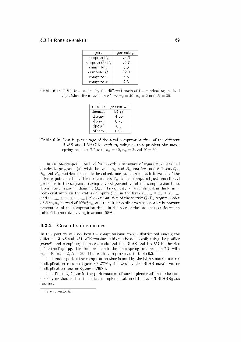
6.3 Performance analysis 69
part percentagecompute Γu 23.6
compute Q · Γu 25.7compute g 9.9compute H 32.9compute u 5.5compute x 2.3
Table 6.1: CPU time needed by the di�erent parts of the condensing methodalgorithm, for a problem of size nx = 40, nu = 2 and N = 30.
routine percentagedgemm 94.77dgemv 4.36dtrsm 0.25dpotrf 0.0others 0.62
Table 6.2: Cost in percentage of the total computation time of the di�erentBLAS and LAPACK routines, using as test problem the mass-spring problem 7.2 with nx = 40, nu = 2 and N = 30.
In an interior-point method framework, a sequence of equality constrainedquadratic programs (all with the same An and Bn matrices and di�erent Qn,Sn and Rn matrices) needs to be solved, one problem at each iteration of theinterior-point method. Then the matrix Γu can be computed just once for allproblems in the sequence, saving a good percentage of the computation time.Even more, in case of diagonal Qn and inequality constraints just in the form ofbox constraints on the states or inputs (i.e. in the form xn,min ≤ xn ≤ xn,max
and un,min ≤ un ≤ un,max), the computation of the matrix Q ·Γu requires orderof N2nxnu instead of N
2n2xnu, and then it is possible to save another important
percentage of the computation time: in the case of the problem considered intable 6.1, the total saving is around 50%.
6.3.2 Cost of sub-routines
In this part we analyze how the computational cost is distributed among thedi�erent BLAS and LAPACK routines: this can be done easily using the pro�lergprof3 and compiling the solver code and the BLAS and LAPACK librariesusing the �ag -pg. The test problem is the mass-spring test problem 7.2, withnx = 40, nu = 2, N = 30. The results are presented in table 6.2.
The major part of the computation time is used by the BLAS matrix-matrixmultiplication routine dgemm (94.77%), followed by the BLAS matrix-vectormultiplication routine dgemv (4.36%).
The limiting factor in the performances of our implementation of the con-densing method is then the e�cient implementation of the level-3 BLAS dgemm
routine.
3See appendix A.
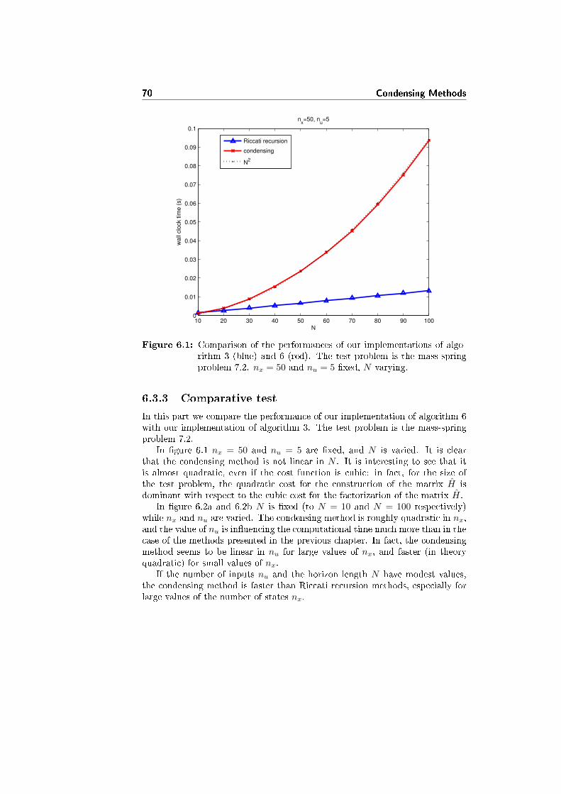
70 Condensing Methods
10 20 30 40 50 60 70 80 90 1000
0.01
0.02
0.03
0.04
0.05
0.06
0.07
0.08
0.09
0.1
nx=50, n
u=5
N
wall
clo
ck tim
e (
s)
Riccati recursion
condensing
N2
Figure 6.1: Comparison of the performances of our implementations of algo-rithm 3 (blue) and 6 (red). The test problem is the mass-springproblem 7.2. nx = 50 and nu = 5 �xed, N varying.
6.3.3 Comparative test
In this part we compare the performance of our implementation of algorithm 6with our implementation of algorithm 3. The test problem is the mass-springproblem 7.2.
In �gure 6.1 nx = 50 and nu = 5 are �xed, and N is varied. It is clearthat the condensing method is not linear in N . It is interesting to see that itis almost quadratic, even if the cost function is cubic: in fact, for the size ofthe test problem, the quadratic cost for the construction of the matrix H isdominant with respect to the cubic cost for the factorization of the matrix H.
In �gure 6.2a and 6.2b N is �xed (to N = 10 and N = 100 respectively)while nx and nu are varied. The condensing method is roughly quadratic in nx,and the value of nu is in�uencing the computational time much more than in thecase of the methods presented in the previous chapter. In fact, the condensingmethod seems to be linear in nu for large values of nx, and faster (in theoryquadratic) for small values of nx.
If the number of inputs nu and the horizon length N have modest values,the condensing method is faster than Riccati recursion methods, especially forlarge values of the number of states nx.
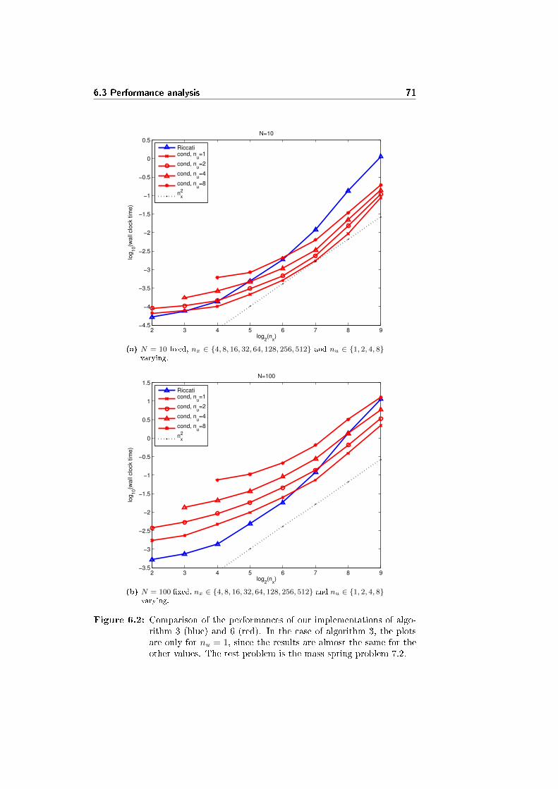
6.3 Performance analysis 71
2 3 4 5 6 7 8 9−4.5
−4
−3.5
−3
−2.5
−2
−1.5
−1
−0.5
0
0.5N=10
log2(n
x)
log
10(w
all
clo
ck tim
e)
Riccaticond, n
u=1
cond, nu=2
cond, nu=4
cond, nu=8
nx
2
(a) N = 10 �xed, nx ∈ {4, 8, 16, 32, 64, 128, 256, 512} and nu ∈ {1, 2, 4, 8}varying.
2 3 4 5 6 7 8 9−3.5
−3
−2.5
−2
−1.5
−1
−0.5
0
0.5
1
1.5N=100
log2(n
x)
log
10(w
all
clo
ck tim
e)
Riccaticond, n
u=1
cond, nu=2
cond, nu=4
cond, nu=8
nx
2
(b) N = 100 �xed, nx ∈ {4, 8, 16, 32, 64, 128, 256, 512} and nu ∈ {1, 2, 4, 8}varying.
Figure 6.2: Comparison of the performances of our implementations of algo-rithm 3 (blue) and 6 (red). In the case of algorithm 3, the plotsare only for nu = 1, since the results are almost the same for theother values. The test problem is the mass-spring problem 7.2.

72 Condensing Methods
Chapter 7
Test problems as Extended
Linear Quadratic Control
Problem
In this chapter we present a test problem as an instance of the extended linearquadratic control problem, and compare the solvers derived in the previouschapters.
7.1 Mass-spring system
7.1.1 Problem de�nition
We use the mass-spring system as test problem for our implementations of thedi�erent methods for the solution of problem 2.1. The mass-spring systemconsists in a chain of p masses (all of value 1) connected by springs (all ofconstant 1); furthermore a spring connects the �rst mass to a wall, and anotherspring connects the last mass to another wall. m forces (inputs) acts on the�rst m masses. This test problem is actually an instance of 2.2, but the solversdeveloped for 2.1 will be used for its solution.
The system can be modeled as the system of p second order linear di�erentialequations
q1 = −2q1 + qq + f1
qi = qi−1 − 2qi + qi+1 + fi, i = 2, . . . ,m
qi = qi−1 − 2qi + qi+1, i = m+ 1, . . . , p− 1
qp = qp−1 − 2qp
where qi is the deviation from the equilibrium point of the i-th mass and fi isthe force acting on the i-th mass.
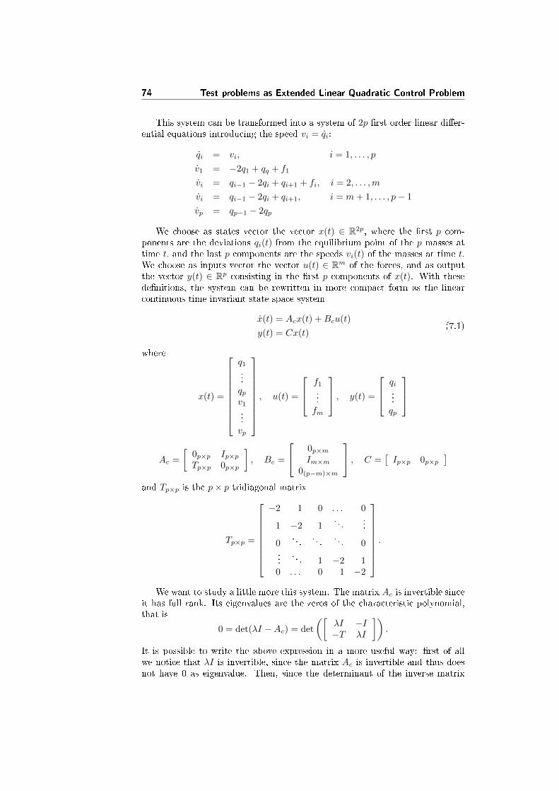
74 Test problems as Extended Linear Quadratic Control Problem
This system can be transformed into a system of 2p �rst order linear di�er-ential equations introducing the speed vi = qi:
qi = vi, i = 1, . . . , p
v1 = −2q1 + qq + f1
vi = qi−1 − 2qi + qi+1 + fi, i = 2, . . . ,m
vi = qi−1 − 2qi + qi+1, i = m+ 1, . . . , p− 1
vp = qp−1 − 2qp
We choose as states vector the vector x(t) ∈ R2p, where the �rst p com-ponents are the deviations qi(t) from the equilibrium point of the p masses attime t, and the last p components are the speeds vi(t) of the masses at time t.We choose as inputs vector the vector u(t) ∈ Rm of the forces, and as outputthe vector y(t) ∈ Rp consisting in the �rst p components of x(t). With thesede�nitions, the system can be rewritten in more compact form as the linearcontinuous time invariant state space system
x(t) = Acx(t) +Bcu(t)
y(t) = Cx(t)(7.1)
where
x(t) =
q1
...qpv1
...vp
, u(t) =
f1
...fm
, y(t) =
qi...qp
Ac =
[0p×p Ip×pTp×p 0p×p
], Bc =
0p×mIm×m
0(p−m)×m
, C =[Ip×p 0p×p
]and Tp×p is the p× p tridiagonal matrix
Tp×p =
−2 1 0 . . . 0
1 −2 1. . .
...
0. . .
. . .. . . 0
.... . . 1 −2 1
0 . . . 0 1 −2
.
We want to study a little more this system. The matrix Ac is invertible sinceit has full rank. Its eigenvalues are the zeros of the characteristic polynomial,that is
0 = det(λI −Ac) = det
([λI −I−T λI
]).
It is possible to write the above expression in a more useful way: �rst of allwe notice that λI is invertible, since the matrix Ac is invertible and thus doesnot have 0 as eigenvalue. Then, since the determinant of the inverse matrix
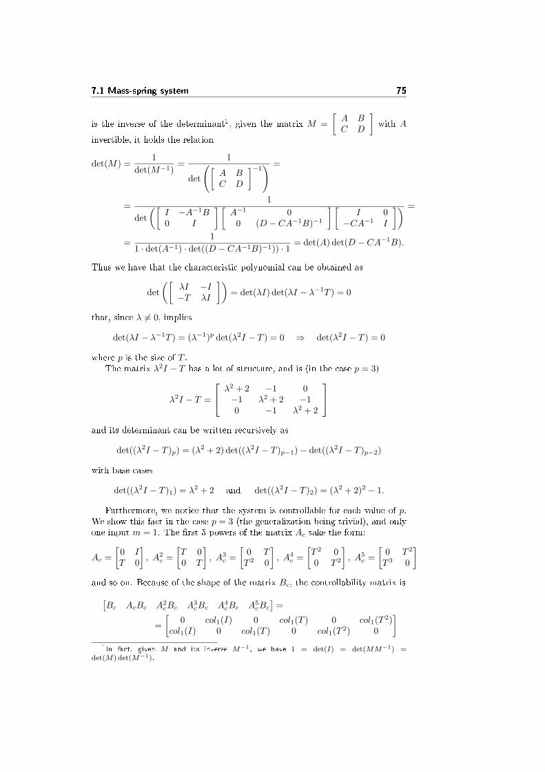
7.1 Mass-spring system 75
is the inverse of the determinant1, given the matrix M =
[A BC D
]with A
invertible, it holds the relation
det(M) =1
det(M−1)=
1
det
([A BC D
]−1) =
=1
det
([I −A−1B0 I
] [A−1 0
0 (D − CA−1B)−1
] [I 0
−CA−1 I
]) =
=1
1 · det(A−1) · det((D − CA−1B)−1)) · 1= det(A) det(D − CA−1B).
Thus we have that the characteristic polynomial can be obtained as
det
([λI −I−T λI
])= det(λI) det(λI − λ−1T ) = 0
that, since λ 6= 0, implies
det(λI − λ−1T ) = (λ−1)p det(λ2I − T ) = 0 ⇒ det(λ2I − T ) = 0
where p is the size of T .The matrix λ2I − T has a lot of structure, and is (in the case p = 3)
λ2I − T =
λ2 + 2 −1 0−1 λ2 + 2 −10 −1 λ2 + 2
and its determinant can be written recursively as
det((λ2I − T )p) = (λ2 + 2) det((λ2I − T )p−1)− det((λ2I − T )p−2)
with base cases
det((λ2I − T )1) = λ2 + 2 and det((λ2I − T )2) = (λ2 + 2)2 − 1.
Furthermore, we notice that the system is controllable for each value of p.We show this fact in the case p = 3 (the generalization being trivial), and onlyone input m = 1. The �rst 5 powers of the matrix Ac take the form:
Ac =
[0 IT 0
], A2
c =
[T 00 T
], A3
c =
[0 TT 2 0
], A4
c =
[T 2 00 T 2
], A5
c =
[0 T 2
T 3 0
]and so on. Because of the shape of the matrix Bc, the controllability matrix is[
Bc AcBc A2cBc A3
cBc A4cBc A5
cBc]
=
=
[0 col1(I) 0 col1(T ) 0 col1(T 2)
col1(I) 0 col1(T ) 0 col1(T 2) 0
]1In fact, given M and its inverse M−1, we have 1 = det(I) = det(MM−1) =
det(M) det(M−1).
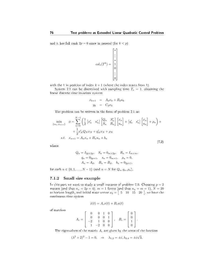
76 Test problems as Extended Linear Quadratic Control Problem
and it has full rank 2p = 6 since in general (for k < p)
col1(T k) =
∗...∗10...0
with the 1 in position of index k + 1 (where the index starts from 1).
System 7.1 can be discretized with sampling time Ts = 1, obtaining thelinear discrete time invariant system
xk+1 = Adxk +Bduk
yk = Cdxk
The problem can be written in the form of problem 2.1 as:
min{un,xn+1}
φ =
N−1∑n=0
(1
2
[x′n u′n
] [Qn S′nSn Rn
] [xnun
]+[q′n s′n
] [xnun
]+ ρn
)+
+1
2x′NQNxN + q′NxN + ρN
s.t. xn+1 = Anxn +Bnun + bn(7.2)
where
Qn = I2p×2p, Sn = 0m×2p, Rn = Im×m,
qn = 02p×1, sn = 0m×1, ρn = 0,
An = Ad, Bn = Bd, bn = 02p×1,
for each n ∈ {0, 1, . . . , N − 1} (and n = N for Qn, qn, ρn).
7.1.2 Small size example
In this part we want to study a small instance of problem 7.2. Choosing p = 2masses (and thus nx = 2p = 4), m = 1 forces (and thus nu = m = 1), N = 20as horizon length, and initial state vector x0 =
[5 10 15 20
], we have the
continuous time system
x(t) = Acx(t) +Bcu(t)
of matrices
Ac =
0 0 1 00 0 0 1−2 1 0 0
1 −2 0 0
, Bc =
0010
.The eigenvalues of the matrix Ac are given by the zeros of the function
(λ2 + 2)2 − 1 = 0, ⇒ λ1,2 = ±i, λ3,4 = ±i√
3,
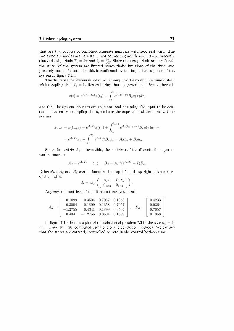
7.1 Mass-spring system 77
that are two couples of complex-conjugate numbers with zero real part. Thetwo associate modes are persistent (not converging nor diverging) and preciselysinusoids of periods T1 = 2π and t2 = 2π√
3. Since the two periods are irrational,
the states of the system are limited non-periodic functions of the time, andprecisely sums of sinusoids: this is con�rmed by the impulsive response of thesystem in �gure 7.1a.
The discrete time system is obtained by sampling the continuous time systemwith sampling time Ts = 1. Remembering that the general solution at time t is
x(t) = eAc(t−t0)x(t0) +
∫ t
t0
eAc(t−τ)Bcu(τ)dτ,
and that the system matrices are constant, and assuming the input to be con-stant between two sampling times, we have the expression of the discrete timesystem
xn+1 = x(tn+1) = eAcTsx(tn) +
∫ tn+1
tn
eAc(tn+1−τ)Bcu(τ)dτ =
= eAcTsxn +
∫ Ts
0
eActdtBcun = Adxn +Bdun.
Since the matrix Ac is invertible, the matrices of the discrete time systemcan be found as
Ad = eAcTs and Bd = A−1c (eAcTs − I)Bc.
Otherwise, Ad and Bd can be found as the top left and top right sub-matricesof the matrix
E = exp
([AcTs BcTs01×2 01×1
]).
Anyway, the matrices of the discrete time system are
Ad =
0.1899 0.3504 0.7057 0.13580.3504 0.1899 0.1358 0.7057−1.2755 0.4341 0.1899 0.3504
0.4341 −1.2755 0.3504 0.1899
, Bd =
0.42330.03640.70570.1358
In �gure 7.1b there is a plot of the solution of problem 7.2 in the case nx = 4,
nu = 1 and N = 20, computed using one of the developed methods. We can seethat the states are correctly controlled to zero in the control horizon time.
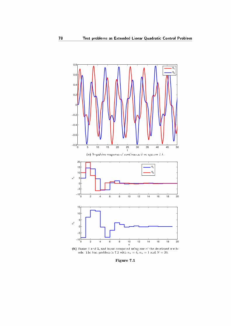
78 Test problems as Extended Linear Quadratic Control Problem
0 5 10 15 20 25 30 35 40 45 50−0.8
−0.6
−0.4
−0.2
0
0.2
0.4
0.6
0.8
t
q
1
q2
(a) Impulsive response of continuous time system 7.1.
0 2 4 6 8 10 12 14 16 18 20−10
−5
0
5
10
15
20
xn
0 2 4 6 8 10 12 14 16 18 20−10
−5
0
5
10
15
n
un
q1
q2
(b) States 1 and 2, and input computed using one of the developed meth-ods. The test problem is 7.2 with nx = 4, nu = 1 and N = 20.
Figure 7.1
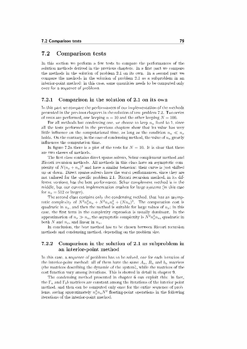
7.2 Comparison tests 79
7.2 Comparison tests
In this section we perform a few tests to compare the performances of thesolution methods derived in the previous chapters. In a �rst part we comparethe methods in the solution of problem 2.1 on its own. In a second part wecompare the methods in the solution of problem 2.1 as a subproblem in aninterior-point method: in this case, some quantities needs to be computed onlyonce for a sequence of problems.
7.2.1 Comparison in the solution of 2.1 on its own
In this part we compare the performances of our implementation of the methodspresented in the previous chapters in the solution of test problem 7.2. Two seriesof tests are performed, one keeping n = 10 and the other keeping N = 100.
For all methods but condensing one, we choose to keep nu �xed to 1, sinceall the tests performed in the previous chapters show that its value has verylittle in�uence on the computational time, as long as the condition nu � nxholds. On the contrary, in the case of condensing method, the value of un greatlyin�uences the computation time.
In �gure 7.2a there is a plot of the tests for N = 10. It is clear that thereare two classes of methods.
The �rst class contains direct sparse solvers, Schur complement method andRiccati recursion methods. All methods in this class have an asymptotic com-plexity of N(nx + nu)3 and have a similar behavior: their curve is just shiftedup or down. Direct sparse solvers have the worst performances, since they arenot tailored for the speci�c problem 2.1. Riccati recursion method, in its dif-ferent versions, has the best performance. Schur complement method is in themiddle, but our current implementation crashes for large systems (in this casefor nx = 512 or larger).
The second class contains only the condensing method, that has an asymp-totic complexity of N2n2
xnu + N2nxn2u + (Nnu)3. The computation cost is
quadratic in nx, and then the method is suitable for large values of nx: in thiscase, the �rst term in the complexity expression is usually dominant. In theapproximation of nx � nu, the asymptotic complexity is N2n2
xnu, quadratic inboth N and nx, and linear in nu.
In conclusion, the best method has to be chosen between Riccati recursionmethods and condensing method, depending on the problem size.
7.2.2 Comparison in the solution of 2.1 as subproblem inan interior-point method
In this case, a sequence of problems has to be solved, one for each iteration ofthe interior-point method: all of them have the same An, Bn and bn matrices(the matrices describing the dynamic of the system), while the matrices of thecost function vary among iterations. This is showed in detail in chapter 9.
The condensing method presented in chapter 6 can exploit this: in fact,the Γu and Γbb matrices are constant among the iterations of the interior-pointmethod, and then can be computed only once for the entire sequence of prob-lems, saving approximately n2
xnuN2 �oating-point operations in the following
iterations of the interior-point method.
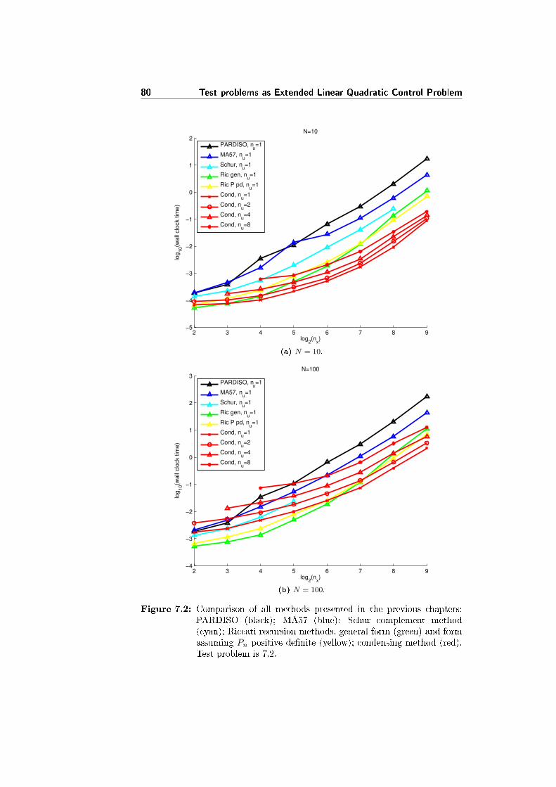
80 Test problems as Extended Linear Quadratic Control Problem
2 3 4 5 6 7 8 9−5
−4
−3
−2
−1
0
1
2N=10
log2(n
x)
log
10(w
all
clo
ck t
ime
)
PARDISO, n
u=1
MA57, nu=1
Schur, nu=1
Ric gen, nu=1
Ric P pd, nu=1
Cond, nu=1
Cond, nu=2
Cond, nu=4
Cond, nu=8
(a) N = 10.
2 3 4 5 6 7 8 9−4
−3
−2
−1
0
1
2
3N=100
log2(n
x)
log
10(w
all
clo
ck t
ime
)
PARDISO, n
u=1
MA57, nu=1
Schur, nu=1
Ric gen, nu=1
Ric P pd, nu=1
Cond, nu=1
Cond, nu=2
Cond, nu=4
Cond, nu=8
(b) N = 100.
Figure 7.2: Comparison of all methods presented in the previous chapters:PARDISO (black); MA57 (blue); Schur complement method(cyan); Riccati recursion methods, general form (green) and formassuming Pn positive de�nite (yellow); condensing method (red).Test problem is 7.2.
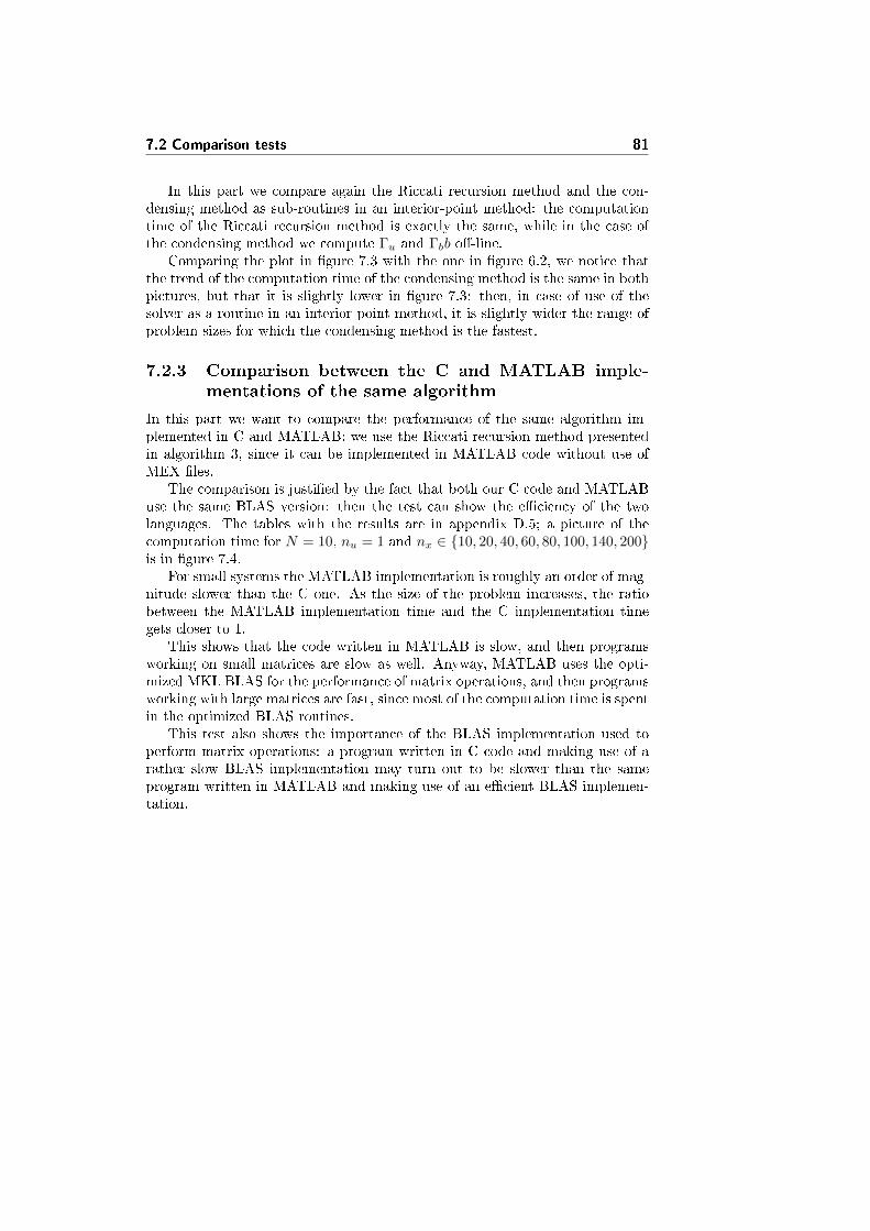
7.2 Comparison tests 81
In this part we compare again the Riccati recursion method and the con-densing method as sub-routines in an interior-point method: the computationtime of the Riccati recursion method is exactly the same, while in the case ofthe condensing method we compute Γu and Γbb o�-line.
Comparing the plot in �gure 7.3 with the one in �gure 6.2, we notice thatthe trend of the computation time of the condensing method is the same in bothpictures, but that it is slightly lower in �gure 7.3: then, in case of use of thesolver as a routine in an interior-point method, it is slightly wider the range ofproblem sizes for which the condensing method is the fastest.
7.2.3 Comparison between the C and MATLAB imple-mentations of the same algorithm
In this part we want to compare the performance of the same algorithm im-plemented in C and MATLAB: we use the Riccati recursion method presentedin algorithm 3, since it can be implemented in MATLAB code without use ofMEX �les.
The comparison is justi�ed by the fact that both our C code and MATLABuse the same BLAS version: then the test can show the e�ciency of the twolanguages. The tables with the results are in appendix D.5; a picture of thecomputation time for N = 10, nu = 1 and nx ∈ {10, 20, 40, 60, 80, 100, 140, 200}is in �gure 7.4.
For small systems the MATLAB implementation is roughly an order of mag-nitude slower than the C one. As the size of the problem increases, the ratiobetween the MATLAB implementation time and the C implementation timegets closer to 1.
This shows that the code written in MATLAB is slow, and then programsworking on small matrices are slow as well. Anyway, MATLAB uses the opti-mized MKL BLAS for the performance of matrix operations, and then programsworking with large matrices are fast, since most of the computation time is spentin the optimized BLAS routines.
This test also shows the importance of the BLAS implementation used toperform matrix operations: a program written in C code and making use of arather slow BLAS implementation may turn out to be slower than the sameprogram written in MATLAB and making use of an e�cient BLAS implemen-tation.
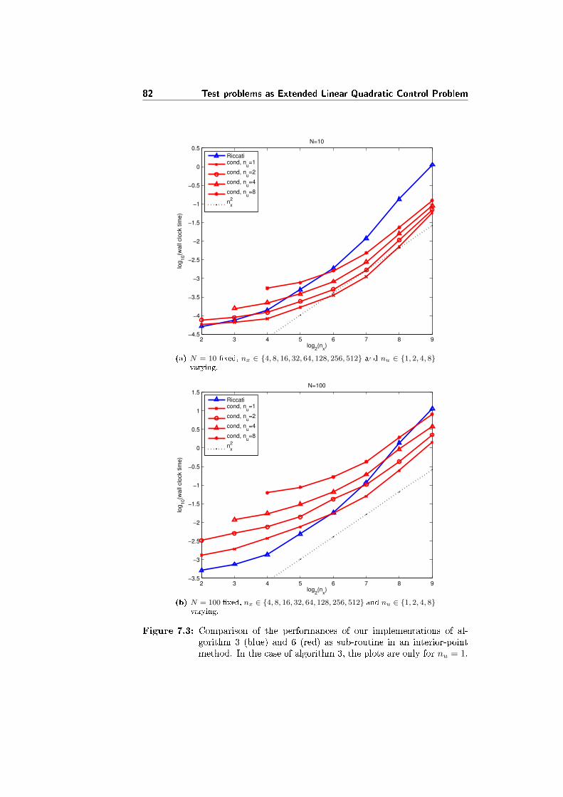
82 Test problems as Extended Linear Quadratic Control Problem
2 3 4 5 6 7 8 9−4.5
−4
−3.5
−3
−2.5
−2
−1.5
−1
−0.5
0
0.5N=10
log2(n
x)
log
10(w
all
clo
ck tim
e)
Riccaticond, n
u=1
cond, nu=2
cond, nu=4
cond, nu=8
nx
2
(a) N = 10 �xed, nx ∈ {4, 8, 16, 32, 64, 128, 256, 512} and nu ∈ {1, 2, 4, 8}varying.
2 3 4 5 6 7 8 9−3.5
−3
−2.5
−2
−1.5
−1
−0.5
0
0.5
1
1.5N=100
log2(n
x)
log
10(w
all
clo
ck tim
e)
Riccaticond, n
u=1
cond, nu=2
cond, nu=4
cond, nu=8
nx
2
(b) N = 100 �xed, nx ∈ {4, 8, 16, 32, 64, 128, 256, 512} and nu ∈ {1, 2, 4, 8}varying.
Figure 7.3: Comparison of the performances of our implementations of al-gorithm 3 (blue) and 6 (red) as sub-routine in an interior-pointmethod. In the case of algorithm 3, the plots are only for nu = 1.
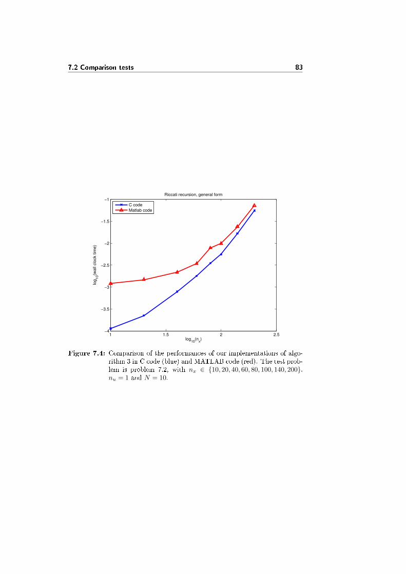
7.2 Comparison tests 83
1 1.5 2 2.5−4
−3.5
−3
−2.5
−2
−1.5
−1
log10
(nx)
log
10(w
all
clo
ck tim
e)
Riccati recursion, general form
C code
Matlab code
Figure 7.4: Comparison of the performances of our implementations of algo-rithm 3 in C code (blue) and MATLAB code (red). The test prob-lem is problem 7.2, with nx ∈ {10, 20, 40, 60, 80, 100, 140, 200},nu = 1 and N = 10.

84 Test problems as Extended Linear Quadratic Control Problem
Chapter 8
Extended Linear Quadratic
Control Problem with
Inequality Constraints
In this chapter we take into consideration an extension of problem 2.1, includingalso inequality constraints together with equality constraints.
8.1 De�nition
In this section we de�ne the extended linear quadratic control problem withinequality constraints, an extension of problem 2.1. The problem is de�ned as
Problem 3. The extended linear quadratic control problem with inequality con-
straints is the quadratic program with equality and inequality constrains
minun,xn+1
φ =
N−1∑n=0
ln(xn, un) + lN (xN )
s.t. xn+1 = Anxn +Bnun + bn
Cnun +Dnxn ≥ dnDNxN ≥ dN
(8.1)
where n ∈ N = {0, 1, . . . , N − 1} and
ln(xn, un) =1
2
[x′n u′n
] [ Qn S′nSn Rn
] [xnun
]+[q′n s′n
] [ xnun
]+ ρn
lN (xN ) =1
2x′NQNxN + q′NxN + ρN
The de�nition of this problem is exactly the same of problem 2.1, a partfrom the presence of the inequality constraints on the state and input.

86 Extended Linear Quadratic Control Problem with Inequality Constraints
8.1.1 Matrix From
Problem 8.1 can be seen as a particular case of the generic quadratic programwith equality and inequality constraints,
minx
φ =1
2x′Hx+ g′x
s.t. Ax = b
Cx ≥ d
(8.2)
where the state vector is
x =
u0
x1
u1
...xN−1
uN−1
xN
and the matrices relative to the cost function and the constraints are
H =
R0
Q1 S′1S1 R1
. . .
QN−1 S′N−1
SN−1 RN−1
QN
, g =
S0x0 + s0
q1
s1
...qN−1
sN−1
qN
A =
−B0 I
−A1 −B1 I. . .
. . .
−AN−1 −BN−1 I
, b =
A0x0 + b0
b1...
bN−1
C =
C0
D1 C1
. . .
DN−1 CN−1
DN
, d =
d0 −D0x0
d1
...dN−1
dN
8.2 Optimality Conditions
In this section we derive optimality conditions for the solution of a generalquadratic program (meaning with this the quadratic program with both equalityand inequality constraints). The general theory can be found in [NW06].
The �rst order necessary optimality conditions for x∗ to be a solution of thequadratic program 8.2 are again the KKT conditions, usually derived from theLagrangian function associated with the quadratic program.
The Lagrangian function of the quadratic program 8.2 takes the form
L = L(x, π, λ) =1
2x′Hx+ g′x− π′(Ax− b)− λ′(Cx− d),
8.2 Optimality Conditions 87
where π and λ are the vectors of the Lagrange multipliers relative to the equalityand inequality constraints.
The �rst order necessary conditions for optimality are the KKT conditions
Hx∗ + g −A′π∗ − C ′λ∗ = 0 (8.3a)
Ax∗ − b = 0 (8.3b)
Cx∗ − d ≥ 0 (8.3c)
λ∗ ≥ 0 (8.3d)
(λ∗)′(Cx∗ − d) = 0 (8.3e)
Because of the conditions on the sign of 8.3c and 8.3d, equation 8.3e impliesthat, if the i-th constraint is active, (Cx∗ − d)i = 0, then the relative Lagrangemultiplier can be positive or null, λi ≥ 0. But, if the i-th constraint is inactive,(Cx∗ − d)i > 0, then the relative Lagrange multiplier has to be null, λi = 0.
The KKT conditions in the form 8.3 are useful for the derivation of interior-point methods in chapter 9. Anyway, for the purposes of this chapter, we preferanother characterization.
Let us denote with E the set of the equality constraints, and with I theset of the inequality constraints. The constraints can be divided into two cate-gories: the active set, containing all the equality constraints and the inequalityconstraints that are active in x∗ (i.e. such that 8.3c is an equality); and theinactive set, containing all the others inequality constraints (i.e. the constraintsthat are inactive in x∗, such that 8.3c is strictly positive). We denote the activeset at the point x∗ as A(x∗).
Furthermore, let us consider the uni�ed notation for both the equality andinequality constraints
Ax− b ≥ 0
where the matrix A and the vector b contains the coe�cient of both the equalityand the inequality constraints. Using the de�nition of active set, we have that,at the point x,
(Ax− b)i = 0 for i ∈ A(x)
(Ax− b)i > 0 for i 6∈ A(x)
The Lagrangian function can be rewritten as
L = L(x, λ) =1
2x′Hx+ g′x− λ′(Ax− b)
and the KKT conditions can be rewritten as
Hx∗ + g −∑
i∈A(x∗)
A′iλ∗i = 0 (8.4a)
(Ax∗ − b)i = 0 for i ∈ A(x∗) (8.4b)
(Ax∗ − b)i > 0 for i 6∈ A(x∗) (8.4c)
λ∗i ≥ 0 for i ∈ I ∩ A(x∗) (8.4d)
where Ai is the i-th row of the matrix A. The meaning of 8.4a is that Hx∗ +g, the gradient of the cost function in x∗, is orthogonal to the constraints inthe active set. Conditions 8.4b and 8.4c imply that the point x∗ is feasible.Condition 8.4d assure that the gradient of the cost function points towards thegrowing half-hyperplane of each inequality constraint in the active set.
88 Extended Linear Quadratic Control Problem with Inequality Constraints
Proposition 8 (First order necessary conditions). If x∗ is a solution for the
quadratic program 8.2, then there exists a vector λ∗ such that the KKT condi-
tions 8.4 hold.
Proof. We show that, if one or more of the conditions 8.4 is not satis�ed, thenthe point x∗ is not a solution for 8.2.
If the point x∗ does not satisfy 8.4b or 8.4c, it is not a feasible point, andthen it is not a solution.
If condition 8.4a is not satis�ed, we can repeat the proof of proposition 1 and�nd a step ∆x = x − x∗ along the active constraints such that φ(x) < φ(x∗).As matrices A and b in the proof of 1 we use the matrices of the constraints inthe active set.
If condition 8.4d is not satis�ed, then λ∗i < 0 for at least one index i ∈ A(x∗).Let us assume that λ∗j < 0. The idea of the proof is that it is possible to �nda small step moving away from the j-th constraint while keeping on the otheractive constraints, and arriving in a feasible point. For a small length of thestep, the cost function decreases.
Let us see the details. Let x be a feasible point such that Aix − bi = 0 fori ∈ A(x∗), i 6= j, and Ajx−bj > 0. Let us de�ne the direction ∆x = x−x∗, andδx = ∆xε, ε > 0 a small step in the direction ∆x. Then Aiδx = (Aix−Aix∗)ε =(bi − bi)ε = 0 for i ∈ A(x∗), i 6= j, and Ajδx = (Ajx−Ajx∗)ε > (bi − bi)ε = 0.
The projection of the gradient of the cost function along the step δx is
δx′(Hx∗ + g) =∑
i∈A(x∗),i6=j
δx′A′iλ∗i + δx′A′jλ
∗j = 0 + ε(Aj∆x)′λ∗j = −εβ < 0
The value of the cost function in the point x = x∗ + δx is
φ(x) = φ(x∗ + δx) = φ(x∗) + δx′(Hx∗ + g) +1
2δx′Hδx = φ(x∗)− βε+
1
2αε2
where α = ∆x′H∆x ∈ R and β > 0.
If α ≤ 0, then φ(x) ≤ φ(x∗) − βε < φ(x∗), and then x∗ is not a globalminimizer.
If α > 0, the quantity 12αε
2 − βε < 0 for ε < 2βα : then, for ε <
2βα , it holds
φ(x) < φ(x∗), and then x∗ is not a global minimizer.
Proposition 9 (First order su�cient conditions). If the point x∗ satis�es theKKT conditions 8.4 with the Lagrangian multiplier λ∗, and the matrix H is
positive semi-de�nite, then x∗ is a global minimizer for the cost function, i.e. a
solution for the quadratic program.
Proof. Let x be any feasible point other than x∗, then Aix = bi for i ∈ E andAix ≥ bi for i ∈ I∩A(x∗). Then the step ∆x = x−x∗ satis�es Ai∆x = bi−bi =0 for i ∈ E and Ai∆x = Aix−Aix∗ ≥ bi − bi = 0 for i ∈ I ∩ A(x∗).
Let us rewrite condition 8.4a as Hx∗ + g =∑i∈E A
′iλ∗i +
∑i∈I∩A(x∗)A
′iλ∗i .
Then
∆x′(Hx∗ + g) =∑i∈E
∆x′A′iλ∗i +
∑i∈I∩A(x∗)
∆x′A′iλ∗i ≥ 0 (8.5)
8.2 Optimality Conditions 89
The value of the cost function in x is
φ(x) =φ(x∗ + ∆x) =1
2(x∗ + ∆x)′H(x∗ + ∆x) + (x∗ + ∆x)′g =
=φ(x∗) + ∆x′(Hx∗ + g) +1
2∆x′H∆x ≥ φ(x∗)
using the positive de�niteness of H and expression 8.5.
Note The geometrical interpretation of 8.5 is that the projection of the gra-dient of the cost function Hx∗ + g on a general feasible step ∆x is positive ornull, and then the cost function keeps steady or increases along the direction of∆x.
Proposition 10 (First order su�cient conditions for uniqueness). If the pointx∗ satis�es the KKT conditions 8.4 with the Lagrangian multiplier λ∗, and the
matrix H is positive de�nite, then x∗ is the unique global minimizer for the costfunction, i.e. the unique solution for the quadratic program.
Proof. The beginning of the proof is as in the previous proposition. The valueof the cost function in x is
φ(x) = φ(x∗) + ∆x′(Hx∗ + g) +1
2∆x′H∆x > φ(x∗)
since H is positive de�nite and ∆x 6= 0 (and then ∆x′H∆x>0) and ∆x′(Hx∗+g) ≥ 0.
Proposition 11 (Second order su�cient conditions for uniqueness). Let the
matrix A be the matrix of the constraints in the active set, and let it have full
row rank. Let Z be a matrix whose columns are a base for the null space of A. Ifthe point x∗ satis�es the KKT conditions 8.4 with the Lagrangian multiplier λ∗,the Hessian matrix H is positive semi-de�nite and the reduced Hessian matrix
Z ′HZ is positive de�nite, then x∗ is the unique global minimizer, i.e. the uniquesolution for the quadratic program.
Proof. Let x∗ be a point satisfying the KKT conditions 8.4 together with theLagrangian multiplier λ∗, and let x be any other feasible point.
If x is on the active constraints, then Aix = bi for i ∈ A(x∗). Let us de�ne∆x = x − x∗ 6= 0, then Ai∆x = Aix − Aix∗ = bi − bi = 0 for i ∈ A(x∗), andthen the vector ∆x is in the null space of the matrix A, and can be written as∆x = Zy, and y 6= 0 since Y has full column rank.
The projection of the gradient of the cost function on the vector ∆x is
∆x′(Hx∗ + g) =∑
i∈A(x∗)
∆x′A′iλ∗i = 0.
The value of the cost function in x is
φ(x) = φ(x∗ + ∆x) = φ(x∗) + ∆x′(Hx∗ + g) +1
2∆x′H∆x =
= φ(x∗) +1
2∆x′H∆x > φ(x∗)
90 Extended Linear Quadratic Control Problem with Inequality Constraints
since H is positive de�nite and y 6= 0.If x is not on the active constraints, let us assume that x is not on the j-th
constraint. This means Ajx > bj , while for the other constraints Aix ≥ bi,i ∈ A(x∗), i 6= j. Let us de�ne the step ∆x = x − x∗, then Aj∆x > 0 andAi∆x ≥ 0, i ∈ A(x∗).
The projection of the gradient of the cost function on the step ∆x is
δx′(Hx∗ + g) = ∆x′A′jλ∗j +
∑i∈A(x∗),i6=j
∆x′A′iλ∗i ≥ ∆x′jA
′jλ∗j > 0
The value of the cost function in x is
φ(x) = φ(x∗ + ∆x) = φ(x∗) + ∆x′(Hx∗ + g) +1
2∆x′H∆x ≥
≥ φ(x∗) + ∆x′(Hx∗ + g) > φ(x∗)
This proves that x∗ is the global minimizer.
Chapter 9
Interior-point methods
In this chapter we present two interior-point methods for the solution of quadraticprograms with both equality and inequality constraints: a basic primal-dualmethod, and one of the best interior-point methods in practice, namely theMehrotra predictor-corrector method. One important result is that, thanks tothe speci�c form of the inequality constraints, problem 2.1 arises as a subprob-lem in an interior-point method for the solution of 8.1.
9.1 Derivation
The presentation of interior-point methods for the solution of a general quadraticprogram can be found also in [NW06].
In this section we derive two interior-point methods for the solution of thequadratic program 8.2:
minx
1
2x′Hx+ g′x
Ax = b
Cx ≥ d
The Mehrotra predictor-corrector method is a development of the basicprimal-dual method: the derivation process for the basic method then coincideswith the �rst part of the derivation process for the Mehrotra's one.
9.1.1 Basic primal-dual method
The algorithm is a solution strategy for the KKT conditions 8.3. Introducingthe vector of the slack variables t = Cx − d ≥ 0 (of length l, the number of
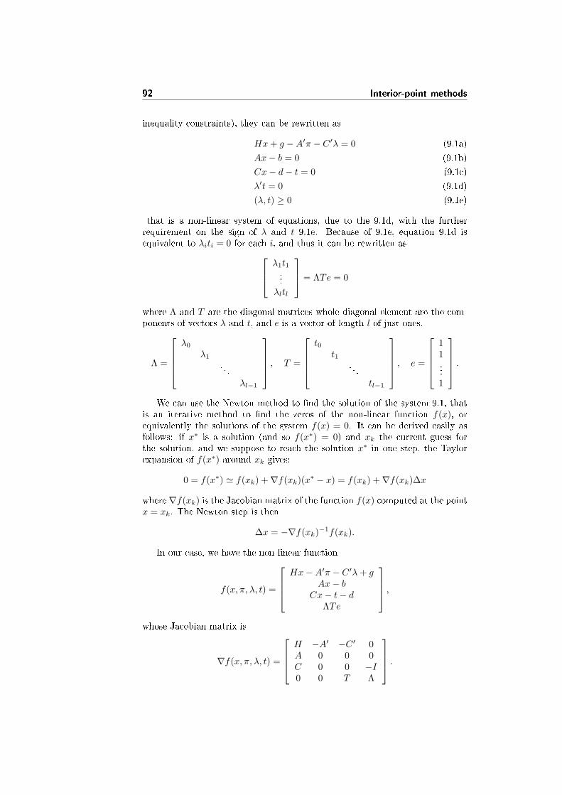
92 Interior-point methods
inequality constraints), they can be rewritten as
Hx+ g −A′π − C ′λ = 0 (9.1a)
Ax− b = 0 (9.1b)
Cx− d− t = 0 (9.1c)
λ′t = 0 (9.1d)
(λ, t) ≥ 0 (9.1e)
that is a non-linear system of equations, due to the 9.1d, with the furtherrequirement on the sign of λ and t 9.1e. Because of 9.1e, equation 9.1d isequivalent to λiti = 0 for each i, and thus it can be rewritten as λ1t1
...λltl
= ΛTe = 0
where Λ and T are the diagonal matrices whole diagonal element are the com-ponents of vectors λ and t, and e is a vector of length l of just ones,
Λ =
λ0
λ1
. . .
λl−1
, T =
t0
t1. . .
tl−1
, e =
11...1
.We can use the Newton method to �nd the solution of the system 9.1, that
is an iterative method to �nd the zeros of the non-linear function f(x), orequivalently the solutions of the system f(x) = 0. It can be derived easily asfollows: if x∗ is a solution (and so f(x∗) = 0) and xk the current guess forthe solution, and we suppose to reach the solution x∗ in one step, the Taylorexpansion of f(x∗) around xk gives:
0 = f(x∗) ' f(xk) +∇f(xk)(x∗ − x) = f(xk) +∇f(xk)∆x
where ∇f(xk) is the Jacobian matrix of the function f(x) computed at the pointx = xk. The Newton step is then
∆x = −∇f(xk)−1f(xk).
In our case, we have the non-linear function
f(x, π, λ, t) =
Hx−A′π − C ′λ+ g
Ax− bCx− t− d
ΛTe
,whose Jacobian matrix is
∇f(x, π, λ, t) =
H −A′ −C ′ 0A 0 0 0C 0 0 −I0 0 T Λ
.
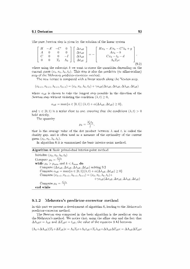
9.1 Derivation 93
The pure Newton step is given by the solution of the linear systemH −A′ −C ′ 0A 0 0 0C 0 0 −I0 0 Tk Λk
∆xaff
∆πaff
∆λaff
∆taff
= −
Hxk −A′πk − C ′λk + g
Axk − bCxk − tk − d
ΛkTke
,(9.2)
where using the subscript k we want to stress the quantities depending on thecurrent guess (xk, πk, λk, tk). This step is also the predictor (or a�ne-scaling)step of the Mehrotra predictor-corrector method.
The new iterate is computed with a linear search along the Newton step,
(xk+1, πk+1, λk+1, tk+1) = (xk, πk, λk, tk) + γαaff(∆xaff ,∆πaff ,∆λaff ,∆taff)
where αaff is chosen to take the longest step possible in the direction of theNewton step without violating the condition (λ, t) ≥ 0,
αaff = max{α ∈ [0, 1] | (λ, t) + α(∆λaff ,∆taff) ≥ 0},
and γ ∈ [0, 1) is a scalar close to one, ensuring that the conditions (λ, t) > 0hold strictly.
The quantity
µk =λ′ktkl,
that is the average value of the dot product between λ and t, is called theduality gap, and is often used as a measure of the optimality of the currentguess (xk, πk, λk, tk).
In algorithm 6 it is summarized the basic interior-point method.
Algorithm 6 Basic primal-dual interior-point method
Initialize (x0, π0, λ0, t0)
Compute µ0 =λ′0t0l
while µk > µmin and k < kmax do
Compute (∆xaff ,∆πaff ,∆λaff ,∆taff) solving 9.2Compute αaff = max{α ∈ [0, 1]|(λ, t) + α(∆λaff ,∆taff) ≥ 0}Compute (xk+1, πk+1, λk+1, tk+1) = (xk, πk, λk, tk)+
+γαaff(∆xaff ,∆πaff ,∆λaff ,∆taff)
Compute µk =λ′ktkl
end while
9.1.2 Mehrotra's predictor-corrector method
In this part we present a development of algorithm 6, leading to the Mehrotra'spredictor-corrector method.
The Newton step computed in the basic algorithm is the predictor step inthe Mehrotra's method. We notice that, using the a�ne step and the fact that∆Λaffe = λaff and ∆Taffe = taff , the value of the equation 9.1d becomes
(Λk+∆Λaff)(Tk+∆Taff)e = ΛkTke+Λktaff+Tkλaff+∆Λaff∆Taffe = ∆Λaff∆Taffe
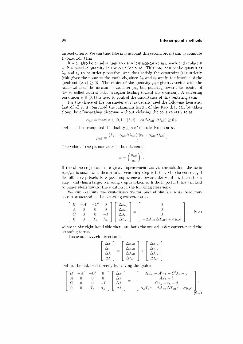
94 Interior-point methods
instead of zero. We can thus take into account this second order term to computea correction term.
It may also be an advantage to use a less aggressive approach and replace 0with a positive quantity in the equation 9.1d. This may ensure the quantitiesλk and tk to be strictly positive, and thus satisfy the constraint 9.1e strictly(this gives the name to the methods, since λk and tk are in the interior of thequadrant (λ, t) ≥ 0). The choice of the quantity µke gives a vector with thesame value of the measure parameter µk, but pointing toward the center ofthe so called central path (a region leading toward the solution). A centeringparameter σ ∈ [0, 1) is used to control the importance of this centering term.
For the choice of the parameter σ, it is usually used the following heuristic:�rst of all it is computed the maximum length of the step that can be takenalong the a�ne-scaling direction without violating the constraints 9.1e as
αaff = max{α ∈ [0, 1] | (λ, t) + α(∆λaff ,∆taff) ≥ 0},
and it is then computed the duality gap of the relative point as
µaff =(λk + αaff∆λaff)′(tk + αaff∆taff)
l.
The value of the parameter σ is thus chosen as
σ =
(µaff
µk
)3
.
If the a�ne step leads to a great improvement toward the solution, the ratioµaff/µk is small, and then a small centering step is taken. On the contrary, ifthe a�ne step leads to a poor improvement toward the solution, the ratio islarge, and thus a larger centering step is taken, with the hope that this will leadto larger steps toward the solution in the following iterations.
We can compute the centering-corrector part of the Mehrotra predictor-corrector method as the centering-corrector step
H −A′ −C ′ 0A 0 0 0C 0 0 −I0 0 Tk Λk
∆xcc
∆πcc
∆λcc
∆tcc
=
000
−∆Λaff∆Taffe+ σµke
, (9.3)
where in the right hand side there are both the second order corrector and thecentering terms.
The overall search direction is∆x∆π∆λ∆t
=
∆xaff
∆πaff
∆λaff
∆taff
+
∆xcc
∆πcc
∆λcc
∆tcc
and can be obtained directly by solving the system
H −A′ −C ′ 0A 0 0 0C 0 0 −I0 0 Tk Λk
∆x∆π∆λ∆t
= −
Hxk −A′πk − C ′λk + g
Axk − bCxk − tk − d
ΛkTke+ ∆Λaff∆Taffe− σµke
,(9.4)
9.1 Derivation 95
The length of the maximum step that can be taken in this direction withoutviolating the constraint 9.1e is
αmax = max{α ∈ [0, 1] | (λk, tk) + αmax(∆λ,∆t) ≥ 0}.
The actual step length is then chosen as
α = γαmax
with γ ∈ (0, 1) to ensure that the condition 9.1e holds strictly; in order toaccelerate convergence, the value of γ may be chosen approaching 1 as thecurrent iterate gets closer to the solution.
We notice that the point (xk+1, πk+1, λk+1, tk+1) = (xk, πk, λk, tk)+α(∆xk,∆πk,∆λk,∆tk)is not feasible with respect to the equality constraints, while, on the contrary,the points (xaff , πaff , λaff , taff) and (xcc, πcc, λcc, tcc) are.
The Mehrotra's predictor-corrector interior-point method is summarized inalgorithm 7.
Algorithm 7 Mehrotra's predictor-corrector interior-point method
Initialize (x0, π0, λ0, t0)
Compute µ0λ′0t0l
while µk > µmin and k < kmax do
Compute (∆xaff ,∆πaff ,∆λaff ,∆taff) solving 9.2Compute αaff = max{α ∈ [0, 1]|(λ, t) + α(∆λaff ,∆taff) ≥ 0}Compute µaff = (λk+αaff∆λaff )
′(tk+αaff∆taff )l
Compute σ = (µaff
µk)3
Compute (∆xcc,∆πcc,∆λcc,∆tcc) solving 9.3Compute (∆xk,∆πk,∆λk,∆tk) = (∆xaff ,∆πaff ,∆λaff ,∆taff)+
+(∆xcc,∆πcc,∆λcc,∆tcc)Compute αmax = max{α ∈ [0, 1]|(λ, t) + α(∆λk,∆tk) ≥ 0}Compute (xk+1, πk+1, λk+1, tk+1) = (xk, πk, λk, tk)+
+γαmax(∆xk,∆πk,∆λk,∆tk)
Compute µk+1 =λ′k+1tk+1
lend while
9.1.3 Computation of the steps as equality constrainedquadratic programs
The most expensive part of the procedure is the computation of the predictorand centering-corrector steps. In this part we show that the computation ofthese two steps is equivalent to the solution of two equality constrained quadraticprograms.
The two linear systems 9.2 and 9.3 have the same matrix, that can be fac-torized just once: then the total cost to compute the two steps is just slightlylarger than the cost to compute one.
It is possible to rewrite the systems in a more useful form. Considering a
96 Interior-point methods
system with a general right hand side in the formH −A′ −C ′ 0A 0 0 0C 0 0 −I0 0 Tk Λk
∆x∆π∆λ∆t
=
rHrArCrT
,we can eliminate the variable ∆t, obtaining H −A′ −C ′
A 0 0ΛkC 0 Tk
∆x∆π∆λ
=
rHrA
rT + ΛkrC
.Finally, by eliminating ∆λ and changing all the signs on the second equation,we get[
H + C ′T−1k ΛkC −A′
−A 0
] [∆x∆π
]=
[rH + C ′T−1
k (rT + ΛkrC)−rA
].
In particular, in order to �nd the predictor step we have to solve system 9.2,that can be rewritten as[
H + C ′T−1k ΛkC −A′
−A 0
] [∆xaff
∆πaff
]=
=
[−((H + C ′T−1
k ΛkC)xk −A′πk + (g − C ′(λk + T−1k Λkd))
)Axk − b
],
that is the KKT system of the equality constrained quadratic program
minx
1
2∆x′aff(H + C ′T−1
k ΛkC)∆xaff+
+(− (H + C ′T−1
k ΛkC)∆xk + g − C ′(λk + T−1k Λkd)
)′∆xaff
s.t. A∆xaff = 0
since the term −A′πk is not in�uencing the value of ∆xaff , but just the one ofthe Lagrangian multiplier ∆πaff .
1
It may be convenient rewrite the KKT system to �nd the iterates instead ofthe steps, as[
H + C ′T−1k ΛkC −A′
−A 0
] [xaff
πaff
]=
[−(g − C ′(λk + T−1
k Λkd))
−b
],
(where xaff = xk + ∆xaff and πaff = πk + ∆πaff) that is the KKT system of theequality constrained quadratic program
minx
1
2x′aff(H + C ′T−1
k ΛkC)xaff + (g − C ′(λk + T−1k Λkd))′xaff
s.t. Axaff = b(9.5)
1In fact, the solution of the KKT system[H −A′−A 0
] [xπ
]= −
[gb
]can be written analiticly, using the Schur complement: π is π = (AH−1A′)−1(b + AH−1g),and thus a term in the form −A′y in g is equivalent to sum −y to the right hand side; x isHx = A′(AH−1A′)−1b+A′(AH−1A′)−1AH−1g− g, and thus a term in the form −A′y in gcancels itself.
9.2 Implementation 97
Similarly, in order to �nd the centering-corrector step we have to solve thesystem 9.3, that can be rewritten as[
H + C ′T−1k ΛkC −A′
−A 0
] [∆xcc
∆πcc
]=
[C ′T−1
k (−∆Λaff∆Taff + σµke)0
],
that is the KKT system of the equality constrained quadratic program
minx
1
2∆x′cc(H + C ′T−1
k ΛkC)∆xcc +(C ′T−1
k (∆Λaff∆Taff − σµke))′
∆xcc
s.t. A∆xcc = 0(9.6)
that, once again, has the same Hessian matrix as 9.5.
9.2 Implementation
In this section we specialize the interior-point methods presented in the previoussection to the speci�c case of problem 8.1. The discussion of interior-pointmethods for the solution of model predictive control problems can be found alsoin [RWR98].
9.2.1 Basic primal-dual methodThe �rst step in the application of algorithm 6 to the case of problem 8.1 is thecomputation of the modi�ed Hessian matrix H = H + C ′(T−1Λ)C (where weare dropping the subscript k to keep the notation simpler). An important result
is that, given the special shape of the C matrix, the modi�ed Hessian matrix Hhas the exact same shape of the Hessian matrix H, namely block diagonal withblock of the same size. For example, in the case N = 3, we have
C′T−1ΛC =
=
C′0
D′1C′1
D′2C′2
D′3
(T−1Λ)0(T−1Λ)1
(T−1Λ)2(T−1Λ)3
C0
D1 C1
D2 C2
D3
=
=
C′0(T−1Λ)0C0
D′1(T−1Λ)1D1 D′1(T−1Λ)1C1
C′1(T−1Λ)1D1 C′1(T−1Λ)1C1
D′2(T−1Λ)2D2 D′2(T−1Λ)2C2
C′2(T−1Λ)2D2 C′2(T−1Λ)2C2
D′3(T−1Λ)3D3
.
Furthermore, the above matrix is symmetric positive semi-de�nite (since itholds (λ, t) ≥ 0, and thus the matrices (T−1Λ)n are diagonal positive semi-de�nite): this means that at each iteration of the interior-point method we haveto solve two problems in the form 2.1, using one of the methods studied in theprevious chapters.
We decide to test our implementations of the interior-point methods usingalgorithm 3 to solve problem 2.1, since this algorithm has shown itself to havegood performances for a wide range of system size.
Algorithm 3 requires the data in the form of the matrices associated to thecost function formulation 2.1, instead of the matrix form 2.3. We thus have
98 Interior-point methods
to compute how these matrices look like. We use for problem 2.1 the notationintroduced in chapter 5.
From the previous discussion about the shape of the matrix C ′(T−1Λ)C, wealready know that
R0 = R0 + C ′0(T−1Λ)0C0
Ri = Ri + C ′i(T−1Λ)iCi i = 1 . . . , N − 1
Si = Si + C ′i(T−1Λ)iDi i = 1 . . . , N − 1
Qi = Qi +D′i(T−1Λ)iDi i = 1 . . . , N − 1
P = P +D′N (T−1Λ)NDN
In the computation of the predictor step, we prefer to solve system 9.5 ob-taining xk instead of ∆xk, and to compute the predictor step as ∆xk = xaff−xk.The linear term of the cost function is
gaff = g − C ′(λ+ (T−1Λ)d) =
=
S0x0 + s0
qis1
q2
s2
p3
−C ′0
D′1C ′1
D′2C ′2
D′3
λ0 + (T−1Λ)0(d0 −D0x0)λ1 + (T−1Λ)1d1
λ2 + (T−1Λ)2d2
λ3 + (T−1Λ)3d3
=
(S0 + (T−1Λ)0C
′0D0)x0 + s0 − C ′0(λ0 + (T−1Λ)0d0)
q1 −D′1(λ1 + (T−1Λ)1d1)s1 − C ′1(λ1 + (T−1Λ)1d1)q2 −D′2(λ2 + (T−1Λ)2d2)s2 − C ′2(λ2 + (T−1Λ)2d2)p3 −D′3(λ3 + (T−1Λ)3d3)
and thus
S0 = S0 + (T−1Λ)0C′0D0, paff = p3 −D′3(λ3 + (T−1Λ)3d3)
and the matrices saff and qaff are
saff =
s0 − C ′0(λ0 + (T−1Λ)0d0)s1 − C ′1(λ1 + (T−1Λ)1d1)s2 − C ′2(λ2 + (T−1Λ)2d2)
, qaff =
q0 −D′0(λ0 + (T−1Λ)0d0)q1 −D′1(λ1 + (T−1Λ)1d1)q2 −D′2(λ2 + (T−1Λ)2d2)
.We notice that from the form of gaff we do not have any information about thevalue of qaff,0, but this is not in�uencing the solution. The value of x0 is thevalue of the system state at the time n = 0.
About the matrices relative to the equality constraints, we notice that theseconstraints are unchanged with respect to the problem formulation 2.1, and thusthe matrices An, Bn, and bn are unchanged.
In the following we show exactly how to compute the di�erent componentsof the predictor step. At each iteration k + 1 of the interior point method, theRiccati recursion algorithm 3 is used to obtain the value of xaff . The relativepredictor step is obtained easily as
∆xaff = xaff − xk.
9.2 Implementation 99
The steps ∆πk and ∆λk are obtained by computing the values πaff and λaff , andby taking the di�erences with respect to the previous values πk and λk. Thevalue of the Lagrangian multiplier πaff is obtained as
πaff,n = qaff,n + Qnxaff,n + S′nuaff,n +A′nπaff,n+1
with initial value
πaff,N = P xaff,N + paff ,
and the step as
∆πaff = πaff − πk.
The value of taff is obtained from equation 9.1c, as
taff = Cxaff − d =
C0uaff,0 +D0x0 − d0
C1uaff,1 +D1xaff,1 − d1
C2uaff,2 +D2xaff,2 − d2
D3xaff,3 − d3
,and then
∆taff = taff − tk.
Finally, the value of ∆λaff is directly obtained as
∆λaff = −T−1k Λk(∆taff + Tke) = −T−1
k Λk(∆taff + tk) = −T−1k Λktaff .
In the following algorithm 8 we present the basic primal-dual interior-pointmethod for the solution of problem 8.1, and we compute the complexity periteration of the interior-point method up to quadratic terms.
The total cost per iteration, considering also the quadratic terms, isN [(4n3x+
6n2xnu + 3nxn
2u + 1
3n3u) + (9n2
x + 9nxnu + 52n
2u) +nl(2n
2x + 2nxnu + 2n2
u + 5nx +5nu)] + 2n2
x + nl(2n2x + 3nx); the asymptotic complexity per iteration is thus
N
[(4n3
x + 6n2xnu + 3nxn
2u +
1
3n3u
)+ nl
(2n2
x + 2nxnu + 2n2u
)].
Using the version 5 of the Riccati recursion, and exploiting the symmetry of thematrices Qn and Rn and the positive semi-de�niteness of the diagonal matrixT−1k Λk, it can be lowered up to
N
[(7
3n3x + 4n2
xnu + 2nxn2u +
1
3n3u
)+ nl
(n2x + 2nxnu + n2
u
)].
Since the number of iterations needed by the interior-point method to convergedepends weakly on the problem size, we have that also the asymptotic complex-ity of the interior-point method is the same.
9.2.2 Mehrotra's predictor-corrector method
In the case of the Mehrotra's predictor-corrector method, we have to computealso the centering-corrector step ∆xcc by solving system 9.6. The linear term
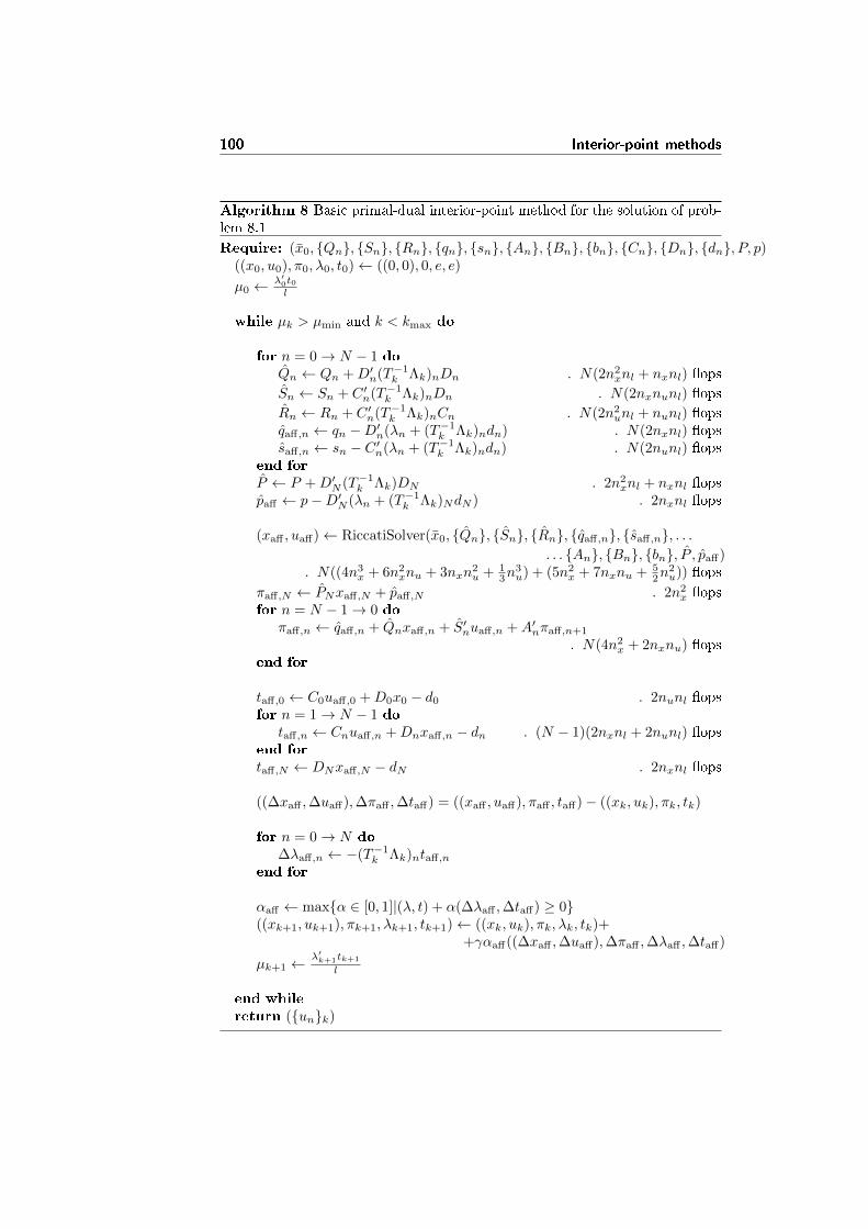
100 Interior-point methods
Algorithm 8 Basic primal-dual interior-point method for the solution of prob-lem 8.1
Require: (x0, {Qn}, {Sn}, {Rn}, {qn}, {sn}, {An}, {Bn}, {bn}, {Cn}, {Dn}, {dn}, P, p)((x0, u0), π0, λ0, t0)← ((0, 0), 0, e, e)
µ0 ← λ′0t0l
while µk > µmin and k < kmax do
for n = 0→ N − 1 doQn ← Qn +D′n(T−1
k Λk)nDn . N(2n2xnl + nxnl) �ops
Sn ← Sn + C ′n(T−1k Λk)nDn . N(2nxnunl) �ops
Rn ← Rn + C ′n(T−1k Λk)nCn . N(2n2
unl + nunl) �opsqaff,n ← qn −D′n(λn + (T−1
k Λk)ndn) . N(2nxnl) �opssaff,n ← sn − C ′n(λn + (T−1
k Λk)ndn) . N(2nunl) �opsend for
P ← P +D′N (T−1k Λk)DN . 2n2
xnl + nxnl �opspaff ← p−D′N (λn + (T−1
k Λk)NdN ) . 2nxnl �ops
(xaff , uaff)← RiccatiSolver(x0, {Qn}, {Sn}, {Rn}, {qaff,n}, {saff,n}, . . .. . . {An}, {Bn}, {bn}, P , paff)
. N((4n3x + 6n2
xnu + 3nxn2u + 1
3n3u) + (5n2
x + 7nxnu + 52n
2u)) �ops
πaff,N ← PNxaff,N + paff,N . 2n2x �ops
for n = N − 1→ 0 doπaff,n ← qaff,n + Qnxaff,n + S′nuaff,n +A′nπaff,n+1
. N(4n2x + 2nxnu) �ops
end for
taff,0 ← C0uaff,0 +D0x0 − d0 . 2nunl �opsfor n = 1→ N − 1 do
taff,n ← Cnuaff,n +Dnxaff,n − dn . (N − 1)(2nxnl + 2nunl) �opsend for
taff,N ← DNxaff,N − dN . 2nxnl �ops
((∆xaff ,∆uaff),∆πaff ,∆taff) = ((xaff , uaff), πaff , taff)− ((xk, uk), πk, tk)
for n = 0→ N do
∆λaff,n ← −(T−1k Λk)ntaff,n
end for
αaff ← max{α ∈ [0, 1]|(λ, t) + α(∆λaff ,∆taff) ≥ 0}((xk+1, uk+1), πk+1, λk+1, tk+1)← ((xk, uk), πk, λk, tk)+
+γαaff((∆xaff ,∆uaff),∆πaff ,∆λaff ,∆taff)
µk+1 ←λ′k+1tk+1
l
end while
return ({un}k)
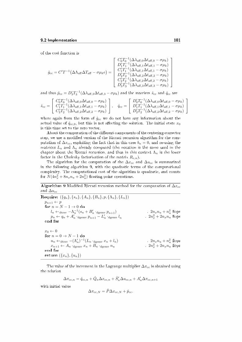
9.2 Implementation 101
of the cost function is
gcc = C ′T−1(∆Λaff∆Taff − σµke
)=
C ′0T−10 (∆λaff,0∆taff,0 − σµk)
D′1T−11 (∆λaff,1∆taff,1 − σµk)
C ′1T−11 (∆λaff,1∆taff,1 − σµk)
D′2T−12 (∆λaff,2∆taff,2 − σµk)
C ′2T−12 (∆λaff,2∆taff,2 − σµk)
D′3T−13 (∆λaff,3∆taff,3 − σµk)
and thus pcc = D′3T
−13 (∆λaff,3∆taff,3 − σµk) and the matrices scc and qcc are
scc =
C ′0T−10 (∆λaff,0∆taff,0 − σµk)
C ′1T−11 (∆λaff,1∆taff,1 − σµk)
C ′2T−12 (∆λaff,2∆taff,2 − σµk)
, qcc =
D′0T−10 (∆λaff,0∆taff,0 − σµk)
D′1T−11 (∆λaff,1∆taff,1 − σµk)
D′2T−12 (∆λaff,2∆taff,2 − σµk)
where again from the form of gcc we do not have any information about theactual value of qcc,0, but this is not a�ecting the solution. The initial state x0
is this time set to the zero vector.About the computation of the di�erent components of the centering-corrector
step, we use a modi�ed version of the Riccati recursion algorithm for the com-putation of ∆xcc, exploiting the fact that in this case bn = 0, and re-using thematrices Ln and Λn already computed (the notation is the same used in thechapter about the Riccati recursion, and thus in this context Λn is the lowerfactor in the Cholesky factorization of the matrix Re,n).
The algorithm for the computation of the ∆xcc and ∆ucc is summarizedin the following algorithm 9, with the quadratic terms of the computationalcomplexity. The computational cost of the algorithm is quadratic, and countsfor N(4n2
x + 8nxnu + 2n2u) �oating-point operations.
Algorithm 9 Modi�ed Riccati recursion method for the computation of ∆xcc
and ∆ucc
Require: ({qn}, {sn}, {An}, {Bn}, p, {Λn}, {Ln})pn+1 ← pfor n = N − 1→ 0 do
ln ←dtrsv −Λ−1n (sn +B′n ·dgemv pn+1) . 2nxnu + n2
u �opspn ← qn +A′n ·dgemv pn+1 − L′n ·dgemv ln . 2n2
x + 2nxnu �opsend for
x0 ← 0for n = 0→ N − 1 do
un ←dtrsv −(Λ′n)−1(Ln ·dgemv xn + ln) . 2nxnu + n2u �ops
xn+1 ← An ·dgemv xn +Bn ·dgemv nu . 2n2x + 2nxnu �ops
end for
return ({xn}, {un})
The value of the increment in the Lagrange multiplier ∆πcc is obtained usingthe relation
∆πcc,n = qcc,n + Qn∆xcc,n + S′n∆ucc,n +A′n∆πcc,n+1
with initial value∆πcc,N = P∆xcc,N + pcc.
102 Interior-point methods
The value of ∆tcc is obtained from the equation
C∆xcc −∆tcc = 0
giving
∆tcc = C∆xcc =
C0∆ucc,0
C1∆ucc,1 +D1∆xcc,1
C2∆ucc,2 +D2∆xcc,2
D3∆xcc,3
.Finally, ∆λcc is obtained from the relation
Tk∆λcc + Λk∆tcc = −∆Λaff∆Taff + σµke
giving∆λcc = −T−1
k Λk∆tcc − T−1k (∆Λaff∆Taff − σµke).
In the following algorithm 10 we present the Mehrotra's predictor-correctorinterior-point method for the solution of problem 8.1. We also compute thecomplexity per iteration up to quadratic terms, that isN [(4n3
x+6n2xnu+3nxn
2u+
13n
3u) + (17n2
x + 19nxnu + 92n
2u) + nl(2n
2x + 2nxnu + 2n2
u + 9nx + 9nu)] + 4n2x +
nl(2n2x + 5nx). This means that each iteration of the Mehrotra's predictor-
corrector interior-point method requires N((8n2x + 10nxnu + 2n2
u) + nl(4nx +4nu)) + 2n2
x + 2nxnl �oating-points operations more compared to the basicprimal-dual interior-point method.
Anyway the asymptotic complexity per iteration is the same as the basicprimal-dual interior-point method (algorithm 8), and is
N
[(4n3
x + 6n2xnu + 3nxn
2u +
1
3n3u
)+ nl
(2n2
x + 2nxnu + 2n2u
)],
just using algorithm 3 for the computation of the a�ne step. This cost can belowered up to
N
[(7
3n3x + 4n2
xnu + 2nxn2u +
1
3n3u
)+ nl
(n2x + 2nxnu + n2
u
)]using algorithm 5.
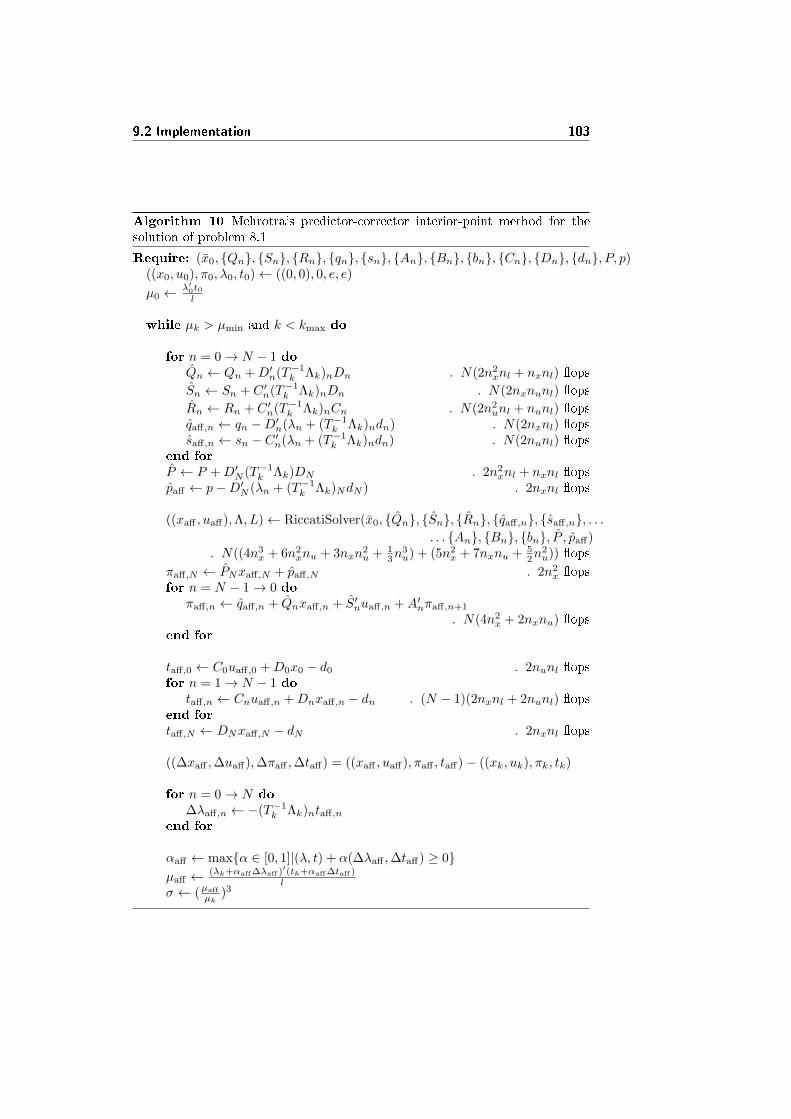
9.2 Implementation 103
Algorithm 10 Mehrotra's predictor-corrector interior-point method for thesolution of problem 8.1
Require: (x0, {Qn}, {Sn}, {Rn}, {qn}, {sn}, {An}, {Bn}, {bn}, {Cn}, {Dn}, {dn}, P, p)((x0, u0), π0, λ0, t0)← ((0, 0), 0, e, e)
µ0 ← λ′0t0l
while µk > µmin and k < kmax do
for n = 0→ N − 1 doQn ← Qn +D′n(T−1
k Λk)nDn . N(2n2xnl + nxnl) �ops
Sn ← Sn + C ′n(T−1k Λk)nDn . N(2nxnunl) �ops
Rn ← Rn + C ′n(T−1k Λk)nCn . N(2n2
unl + nunl) �opsqaff,n ← qn −D′n(λn + (T−1
k Λk)ndn) . N(2nxnl) �opssaff,n ← sn − C ′n(λn + (T−1
k Λk)ndn) . N(2nunl) �opsend for
P ← P +D′N (T−1k Λk)DN . 2n2
xnl + nxnl �opspaff ← p−D′N (λn + (T−1
k Λk)NdN ) . 2nxnl �ops
((xaff , uaff),Λ, L)← RiccatiSolver(x0, {Qn}, {Sn}, {Rn}, {qaff,n}, {saff,n}, . . .. . . {An}, {Bn}, {bn}, P , paff)
. N((4n3x + 6n2
xnu + 3nxn2u + 1
3n3u) + (5n2
x + 7nxnu + 52n
2u)) �ops
πaff,N ← PNxaff,N + paff,N . 2n2x �ops
for n = N − 1→ 0 doπaff,n ← qaff,n + Qnxaff,n + S′nuaff,n +A′nπaff,n+1
. N(4n2x + 2nxnu) �ops
end for
taff,0 ← C0uaff,0 +D0x0 − d0 . 2nunl �opsfor n = 1→ N − 1 do
taff,n ← Cnuaff,n +Dnxaff,n − dn . (N − 1)(2nxnl + 2nunl) �opsend for
taff,N ← DNxaff,N − dN . 2nxnl �ops
((∆xaff ,∆uaff),∆πaff ,∆taff) = ((xaff , uaff), πaff , taff)− ((xk, uk), πk, tk)
for n = 0→ N do
∆λaff,n ← −(T−1k Λk)ntaff,n
end for
αaff ← max{α ∈ [0, 1]|(λ, t) + α(∆λaff ,∆taff) ≥ 0}µaff ← (λk+αaff∆λaff )
′(tk+αaff∆taff )l
σ ← (µaff
µk)3
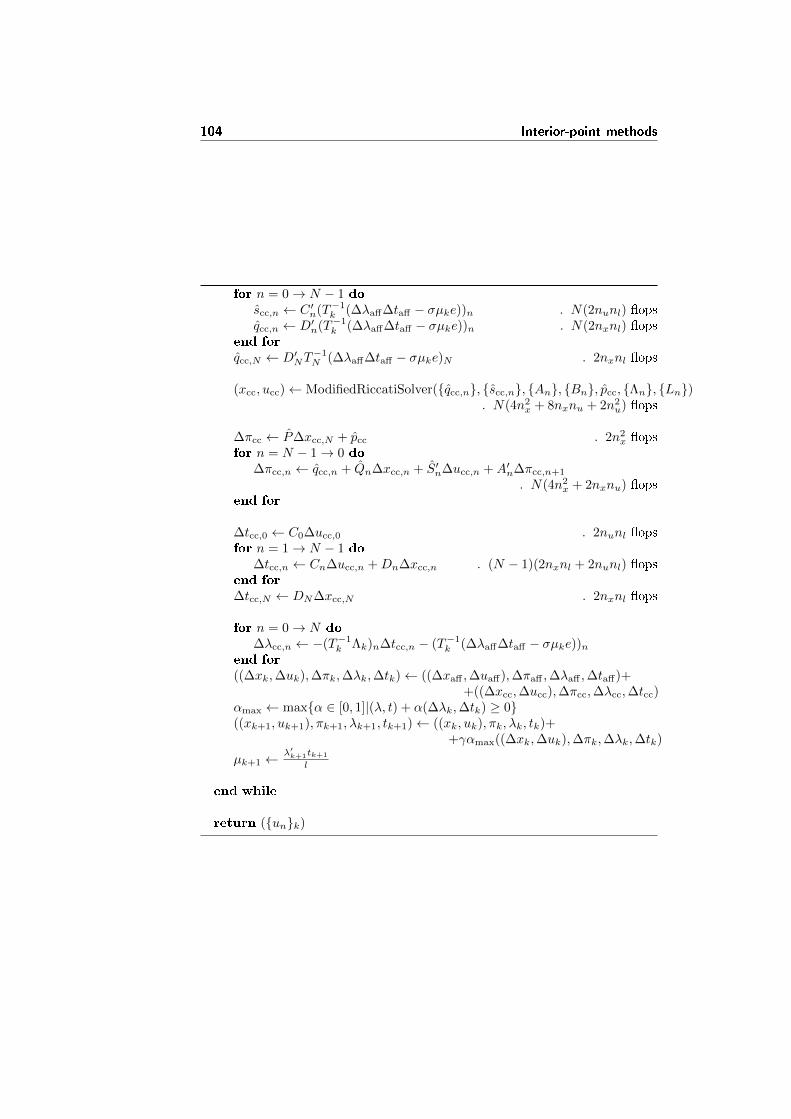
104 Interior-point methods
for n = 0→ N − 1 doscc,n ← C ′n(T−1
k (∆λaff∆taff − σµke))n . N(2nunl) �opsqcc,n ← D′n(T−1
k (∆λaff∆taff − σµke))n . N(2nxnl) �opsend for
qcc,N ← D′NT−1N (∆λaff∆taff − σµke)N . 2nxnl �ops
(xcc, ucc)← ModifiedRiccatiSolver({qcc,n}, {scc,n}, {An}, {Bn}, pcc, {Λn}, {Ln}). N(4n2
x + 8nxnu + 2n2u) �ops
∆πcc ← P∆xcc,N + pcc . 2n2x �ops
for n = N − 1→ 0 do∆πcc,n ← qcc,n + Qn∆xcc,n + S′n∆ucc,n +A′n∆πcc,n+1
. N(4n2x + 2nxnu) �ops
end for
∆tcc,0 ← C0∆ucc,0 . 2nunl �opsfor n = 1→ N − 1 do
∆tcc,n ← Cn∆ucc,n +Dn∆xcc,n . (N − 1)(2nxnl + 2nunl) �opsend for
∆tcc,N ← DN∆xcc,N . 2nxnl �ops
for n = 0→ N do
∆λcc,n ← −(T−1k Λk)n∆tcc,n − (T−1
k (∆λaff∆taff − σµke))nend for
((∆xk,∆uk),∆πk,∆λk,∆tk)← ((∆xaff ,∆uaff),∆πaff ,∆λaff ,∆taff)++((∆xcc,∆ucc),∆πcc,∆λcc,∆tcc)
αmax ← max{α ∈ [0, 1]|(λ, t) + α(∆λk,∆tk) ≥ 0}((xk+1, uk+1), πk+1, λk+1, tk+1)← ((xk, uk), πk, λk, tk)+
+γαmax((∆xk,∆uk),∆πk,∆λk,∆tk)
µk+1 ←λ′k+1tk+1
l
end while
return ({un}k)
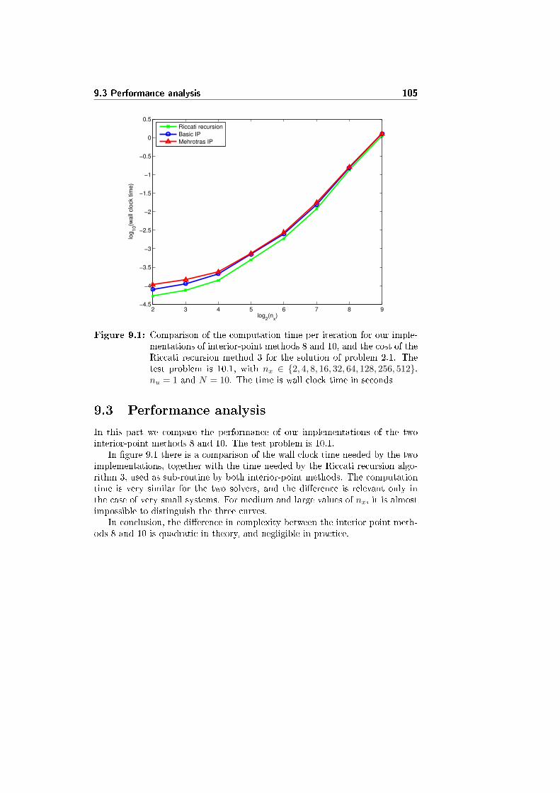
9.3 Performance analysis 105
2 3 4 5 6 7 8 9−4.5
−4
−3.5
−3
−2.5
−2
−1.5
−1
−0.5
0
0.5
log2(n
x)
log
10(w
all
clo
ck t
ime
)
Riccati recursion
Basic IP
Mehrotras IP
Figure 9.1: Comparison of the computation time per iteration for our imple-mentations of interior-point methods 8 and 10, and the cost of theRiccati recursion method 3 for the solution of problem 2.1. Thetest problem is 10.1, with nx ∈ {2, 4, 8, 16, 32, 64, 128, 256, 512},nu = 1 and N = 10. The time is wall clock time in seconds
9.3 Performance analysis
In this part we compare the performance of our implementations of the twointerior-point methods 8 and 10. The test problem is 10.1.
In �gure 9.1 there is a comparison of the wall clock time needed by the twoimplementations, together with the time needed by the Riccati recursion algo-rithm 3, used as sub-routine by both interior-point methods. The computationtime is very similar for the two solvers, and the di�erence is relevant only inthe case of very small systems. For medium and large values of nx, it is almostimpossible to distinguish the three curves.
In conclusion, the di�erence in complexity between the interior point meth-ods 8 and 10 is quadratic in theory, and negligible in practice.

106 Interior-point methods
Chapter 10
Test Problems as Extended
Linear Quadratic Control
Problem with Inequality
Constraints
In this chapter we de�ne a test problem as an instance of problem 8.1, and wecompare each other the performances of the two interior-point methods (algo-rithms 8 and 10) in the solution of this problem.
10.1 Problem de�nition
The test problem is the mass-spring problem with inequality constraints. Theproblem de�nition is the same that in the case of the mass-spring problemconsidered as an instance of problem 2.1, with the di�erence that there are alsoconstraints on the maximum absolute value of the input action.
In fact, the input has to satisfy the constraints
−umax ≤ un ≤ umax
for n ∈ {0, 1, . . . , N − 1}, where umax is the maximum absolute value of theinput. The relation can be written as
{un ≥ −umax
−un ≥ −umax⇒
[I−I
]un ≥
[−I−I
]umax.
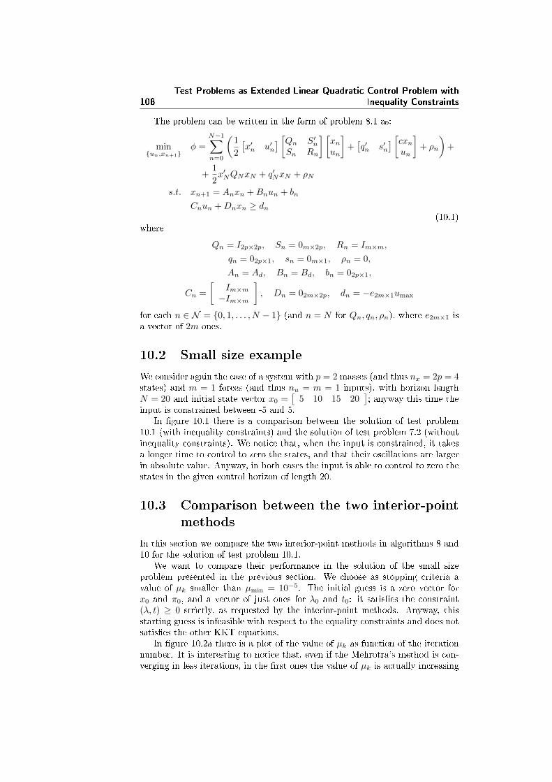
108
Test Problems as Extended Linear Quadratic Control Problem with
Inequality Constraints
The problem can be written in the form of problem 8.1 as:
min{un,xn+1}
φ =
N−1∑n=0
(1
2
[x′n u′n
] [Qn S′nSn Rn
] [xnun
]+[q′n s′n
] [cxnun
]+ ρn
)+
+1
2x′NQNxN + q′NxN + ρN
s.t. xn+1 = Anxn +Bnun + bn
Cnun +Dnxn ≥ dn(10.1)
where
Qn = I2p×2p, Sn = 0m×2p, Rn = Im×m,
qn = 02p×1, sn = 0m×1, ρn = 0,
An = Ad, Bn = Bd, bn = 02p×1,
Cn =
[Im×m−Im×m
], Dn = 02m×2p, dn = −e2m×1umax
for each n ∈ N = {0, 1, . . . , N − 1} (and n = N for Qn, qn, ρn), where e2m×1 isa vector of 2m ones.
10.2 Small size example
We consider again the case of a system with p = 2 masses (and thus nx = 2p = 4states) and m = 1 forces (and thus nu = m = 1 inputs), with horizon lengthN = 20 and initial state vector x0 =
[5 10 15 20
]; anyway this time the
input is constrained between -5 and 5.In �gure 10.1 there is a comparison between the solution of test problem
10.1 (with inequality constraints) and the solution of test problem 7.2 (withoutinequality constraints). We notice that, when the input is constrained, it takesa longer time to control to zero the states, and that their oscillations are largerin absolute value. Anyway, in both cases the input is able to control to zero thestates in the given control horizon of length 20.
10.3 Comparison between the two interior-point
methods
In this section we compare the two interior-point methods in algorithms 8 and10 for the solution of test problem 10.1.
We want to compare their performance in the solution of the small sizeproblem presented in the previous section. We choose as stopping criteria avalue of µk smaller than µmin = 10−5. The initial guess is a zero vector forx0 and π0, and a vector of just ones for λ0 and t0: it satis�es the constraint(λ, t) ≥ 0 strictly, as requested by the interior-point methods. Anyway, thisstarting guess is infeasible with respect to the equality constraints and does notsatis�es the other KKT equations.
In �gure 10.2a there is a plot of the value of µk as function of the iterationnumber. It is interesting to notice that, even if the Mehrotra's method is con-verging in less iterations, in the �rst ones the value of µk is actually increasing
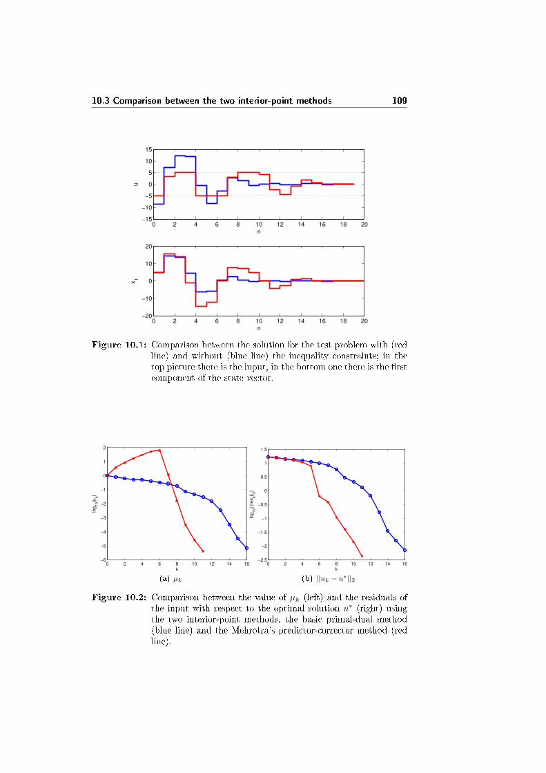
10.3 Comparison between the two interior-point methods 109
0 2 4 6 8 10 12 14 16 18 20−15
−10
−5
0
5
10
15
n
u
0 2 4 6 8 10 12 14 16 18 20−20
−10
0
10
20
n
x1
Figure 10.1: Comparison between the solution for the test problem with (redline) and without (blue line) the inequality constraints; in thetop picture there is the input, in the bottom one there is the �rstcomponent of the state vector.
0 2 4 6 8 10 12 14 16−6
−5
−4
−3
−2
−1
0
1
2
k
log
10(µ
k)
(a) µk
0 2 4 6 8 10 12 14 16−2.5
−2
−1.5
−1
−0.5
0
0.5
1
1.5
k
log
10(|
|res
k||
2)
(b) ||uk − u∗||2
Figure 10.2: Comparison between the value of µk (left) and the residuals ofthe input with respect to the optimal solution u∗ (right) usingthe two interior-point methods, the basic primal-dual method(blue line) and the Mehrotra's predictor-corrector method (redline).
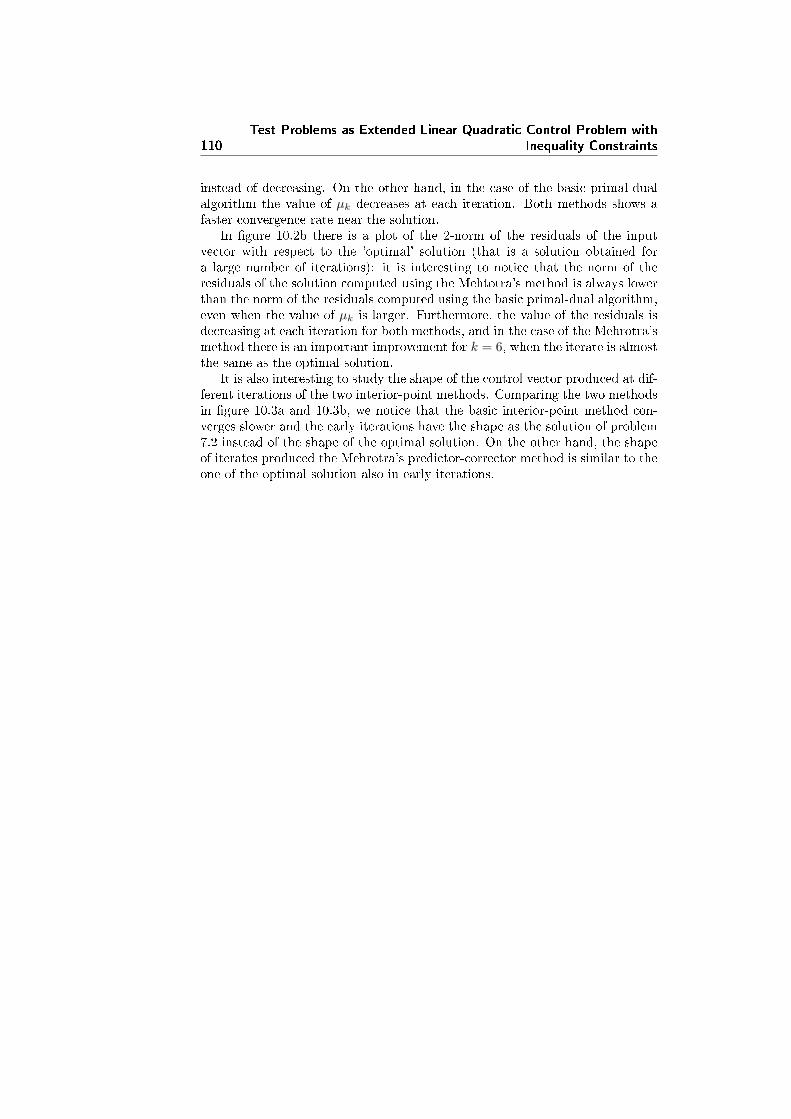
110
Test Problems as Extended Linear Quadratic Control Problem with
Inequality Constraints
instead of decreasing. On the other hand, in the case of the basic primal-dualalgorithm the value of µk decreases at each iteration. Both methods shows afaster convergence rate near the solution.
In �gure 10.2b there is a plot of the 2-norm of the residuals of the inputvector with respect to the 'optimal' solution (that is a solution obtained fora large number of iterations): it is interesting to notice that the norm of theresiduals of the solution computed using the Mehtotra's method is always lowerthan the norm of the residuals computed using the basic primal-dual algorithm,even when the value of µk is larger. Furthermore, the value of the residuals isdecreasing at each iteration for both methods, and in the case of the Mehrotra'smethod there is an important improvement for k = 6, when the iterate is almostthe same as the optimal solution.
It is also interesting to study the shape of the control vector produced at dif-ferent iterations of the two interior-point methods. Comparing the two methodsin �gure 10.3a and 10.3b, we notice that the basic interior-point method con-verges slower and the early iterations have the shape as the solution of problem7.2 instead of the shape of the optimal solution. On the other hand, the shapeof iterates produced the Mehrotra's predictor-corrector method is similar to theone of the optimal solution also in early iterations.
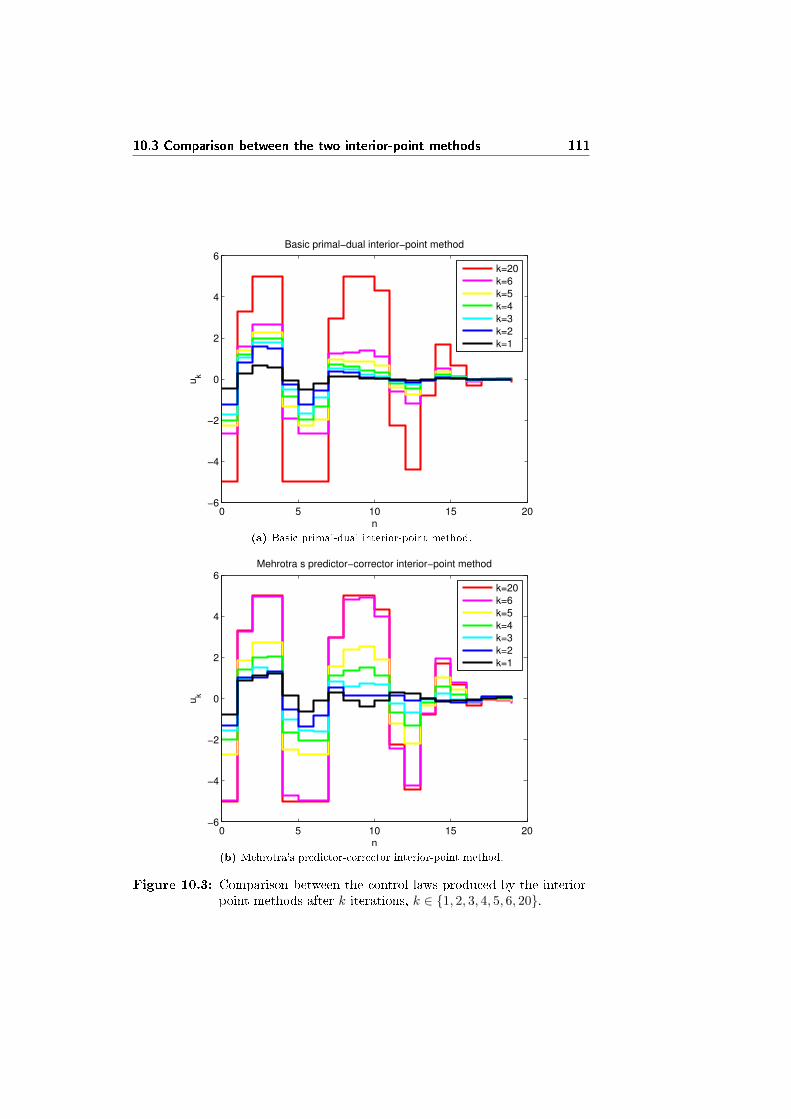
10.3 Comparison between the two interior-point methods 111
0 5 10 15 20−6
−4
−2
0
2
4
6
n
uk
Basic primal−dual interior−point method
k=20
k=6
k=5
k=4
k=3
k=2
k=1
(a) Basic primal-dual interior-point method.
0 5 10 15 20−6
−4
−2
0
2
4
6
n
uk
Mehrotra s predictor−corrector interior−point method
k=20
k=6
k=5
k=4
k=3
k=2
k=1
(b) Mehrotra's predictor-corrector interior-point method.
Figure 10.3: Comparison between the control laws produced by the interior-point methods after k iterations, k ∈ {1, 2, 3, 4, 5, 6, 20}.
112
Test Problems as Extended Linear Quadratic Control Problem with
Inequality Constraints
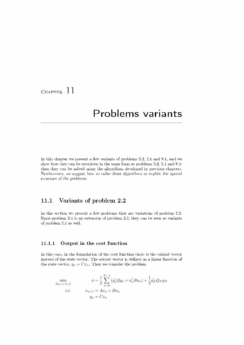
Chapter 11
Problems variants
In this chapter we present a few variants of problems 2.2, 2.1 and 8.1, and weshow how they can be rewritten in the same form as problems 2.2, 2.1 and 8.1:then they can be solved using the algorithms developed in previous chapters.Furthermore, we suggest how to tailor these algorithms to exploit the specialstructure of the problems.
11.1 Variants of problem 2.2
In this section we present a few problems that are variations of problem 2.2.Since problem 2.1 is an extension of problem 2.2, they can be seen as variantsof problem 2.1 as well.
11.1.1 Output in the cost function
In this case, in the formulation of the cost function there is the output vectorinstead of the state vector. The output vector is de�ned as a linear function ofthe state vector, yn = Cxn. Then we consider the problem
min{yn+1,un}
φ =1
2
N−1∑n=0
(y′nQyn + u′nRun) +1
2y′NQNyN
s.t. xn+1 = Axn +Bun
yn = Cxn
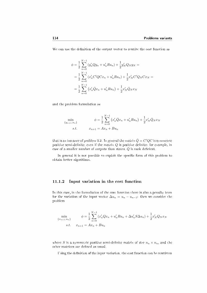
114 Problems variants
We can use the de�nition of the output vector to rewrite the cost function as
φ =1
2
N−1∑n=0
(y′nQyn + u′nRun) +1
2y′NQNyN =
=1
2
N−1∑n=0
(x′nC′QCxn + u′nRun) +
1
2x′NC
′QNCxN =
=1
2
N−1∑n=0
(x′nQxn + u′nRun
)+
1
2x′N QNxN
and the problem formulation as
min{yn+1,un}
φ =1
2
N−1∑n=0
(x′nQxn + u′nRun
)+
1
2x′N QNxN
s.t. xn+1 = Axn +Bun
that is an instance of problem 2.2. In general the matrix Q = C ′QC is symmetricpositive semi-de�nite, even if the matrix Q is positive de�nite: for example, incase of a smaller number of outputs than states, Q is rank de�cient.
In general it is not possible to exploit the speci�c form of this problem toobtain better algorithms.
11.1.2 Input variation in the cost function
In this case, in the formulation of the cost function there is also a penalty termfor the variation of the input vector ∆un = un − un−1: then we consider theproblem
min{xn+1,un}
φ =1
2
N−1∑n=0
(x′nQxn + u′nRun + ∆u′nS∆un) +1
2x′NQNxN
s.t. xn+1 = Axn +Bun
where S is a symmetric positive semi-de�nite matrix of size nu × nu, and theother matrices are de�ned as usual.
Using the de�nition of the input variation, the cost function can be rewritten
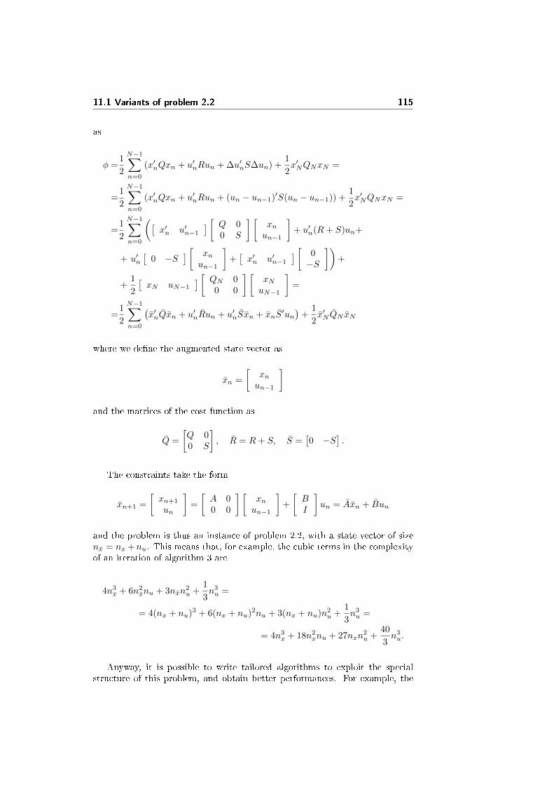
11.1 Variants of problem 2.2 115
as
φ =1
2
N−1∑n=0
(x′nQxn + u′nRun + ∆u′nS∆un) +1
2x′NQNxN =
=1
2
N−1∑n=0
(x′nQxn + u′nRun + (un − un−1)′S(un − un−1)) +1
2x′NQNxN =
=1
2
N−1∑n=0
([x′n u′n−1
] [ Q 00 S
] [xnun−1
]+ u′n(R+ S)un+
+ u′n[
0 −S] [ xn
un−1
]+[x′n u′n−1
] [ 0−S
])+
+1
2
[xN uN−1
] [ QN 00 0
] [xNuN−1
]=
=1
2
N−1∑n=0
(x′nQxn + u′nRun + u′nSxn + xnS
′un)
+1
2x′N QN xN
where we de�ne the augmented state vector as
xn =
[xnun−1
]
and the matrices of the cost function as
Q =
[Q 00 S
], R = R+ S, S =
[0 −S
].
The constraints take the form
xn+1 =
[xn+1
un
]=
[A 00 0
] [xnun−1
]+
[BI
]un = Axn + Bun
and the problem is thus an instance of problem 2.2, with a state vector of sizenx = nx +nu. This means that, for example, the cubic terms in the complexityof an iteration of algorithm 3 are
4n3x + 6n2
xnu + 3nxn2u +
1
3n3u =
= 4(nx + nu)3 + 6(nx + nu)2nu + 3(nx + nu)n2u +
1
3n3u =
= 4n3x + 18n2
xnu + 27nxn2u +
40
3n3u.
Anyway, it is possible to write tailored algorithms to exploit the specialstructure of this problem, and obtain better performances. For example, the
116 Problems variants
Riccati recursion expression is
Pn−1 = Q+ A′PnA− (S + B′PnA)′(R+ B′PnB)−1(S + B′PnA) =
=
[Q 00 S
]+
[A′ 00 0
] [Pn,11 Pn,12
Pn,21 Pn.22
] [A 00 0
]−
−([
0 −S]
+[B′ I
] [ Pn,11 Pn,12
Pn,21 Pn,22
] [A 00 0
])′·
·(
(R+ S) +[B′ I
] [ Pn,11 Pn,12
Pn,21 Pn,22
] [BI
])·
·([
0 −S]
+[B′ I
] [ Pn,11 Pn,12
Pn,21 Pn,22
] [A 00 0
])=
=
[Q 00 S
]+
[A′Pn,11A 0
0 0
]−[A′(Pn,11B + P ′n,21)
−S
]·
· (R+ S +B′Pn,11B +B′Pn,12 + Pn,21B + Pn,22)−1 [
(B′Pn,11 + Pn,21)A −S]
and then algorithm 3 can be modi�ed to implement the above recursion, ob-taining a complexity per iteration with cubic terms
4n3x + 6n2
xnu + 9nxn2u +
10
3n3u,
that is just 6nxn2u + 3n3
u larger than problem 2.2.
11.1.3 Diagonal Hessian in the cost function
This is a special case of problem 2.2, and some of the algorithms presented inthe previous chapeters can take advantage of this.
Riccati recursion method In the case of this method, a diagonal Hessianin not in�uencing the cubic terms in the complexity expression.
Schur complement method This method can take advantage of a diagonalHessian (that has to be positive de�nite). In fact the Cholesky factorization,the inversion of the factor U and the computation of Φ = AU−1 are trivial, andrequire at most a quadratic number of �oating-point operations.
The matrix φ is in the form
Φ =
Φ0,22 Φ1,11
Φ1,21 Φ1,22 Φ2,11
Φ2,21 Φ2,22 Φ3,11
where the Φn,11 are diagonal nx × nx matrices, Φn,21 are full nx × nx matricesand Φn,22 are full nx × nu matrices.
Then the computation of the product Ψ = ΦΦ′ has an asymptotic cost ofN(n3
x+n2xnu) �oating-point operations. The blocks Ψi,j are all dense, and thus
the Cholesky factorization of the matrix Ψ has an asymptotic cost of N( 73n
3x)
�oating-point operations, as usual. The following operations (systems solution)have only a quadratic cost.
11.2 Variants of problem 2.1 117
The asymptotic cost of the algorithm is then
N
(10
3n3x + n2
xnu
).
It is pretty smaller than the cost of the general Schur complement algorithmbut still larger that the most e�cient version of the Riccati recursion methodin the case of nx � nu. Anyway, in case of large value of nu, the algorithm isextremely convenient, being linear in the number of inputs.
Condensing methods Condensing methods can take advantage of a diago-nal Hessian matrix: in this case the computation of the product QΓu has anasymptotic cost of 1
2N2nunx �oating-point operations instead of N2n2
xnu. Theasymptotic cost of the algorithm becomes
2N2nxnu(nx + nu) +1
3(Nnu)3
�oating-point operations.
11.2 Variants of problem 2.1
In this section we present a problem that can be rewritten in the form of problem2.1.
11.2.1 Control to a non-zero reference
In this part we consider the problem of control the states vector to a non-zeroreference,
minxn+1,un
φ =1
2
N−1∑n=0
(xn − zn)′Q(xn − zn) + u′nRun +1
2(xN − zN )′QN (xN − zN )
s.t. xn+1 = Axn +Bun
The cost function can be rewritten as
φ =
N−1∑n=0
(1
2x′nQxn +
1
2u′nRun + (−z′nQ)xn +
1
2z′nQzn
)+
+1
2x′NQNxN + (−z′NQN )xN +
1
2z′NQNzN
that can be seen as the cost function of problem 2.1 with qn = −Qzn andqN = −QNzN .
No special algorithm can be developed.
11.3 Variants of problem 8.1
11.3.1 Diagonal Hessian matrix in the cost function andbox constraints
In this part we study a special case of problem 8.1, namely the case with diagonalHessian in the cost function and box constraints.
118 Problems variants
Box constraints are in the form
umin ≤ un ≤ umax
xmin ≤ xn ≤ xmax
and can be rewritten as
Cnun +Dnxn =
I−I00
un +
00I−I
xn ≥umin
−umax
xmin
−xmax
= dn.
The matrix C ′(T−1Λ)C, that is the update term of the Hessian matrix ateach iteration of the interior-pint method, is diagonal. In fact, for each block i,we have
D′i(T−1Λ)iDi =
=[0 0 I −I
] (T−1Λ)i,1
(T−1Λ)i,2(T−1Λ)i,3
(T−1Λ)i,4
00I−I
=
= (T−1Λ)i,3 + (T−1Λ)i,4
C ′i(T−1Λ)iCi =
=[I −I 0 0
] (T−1Λ)i,1
(T−1Λ)i,2(T−1Λ)i,3
(T−1Λ)i,4
I−I00
=
= (T−1Λ)i,1 + (T−1Λ)i,2
D′i(T−1Λ)iCi =
=[0 0 I −I
] (T−1Λ)i,1
(T−1Λ)i,2(T−1Λ)i,3
(T−1Λ)i,4
I−I00
= 0
then the matrix C ′(T−1Λ)C is diagonal, since the matrix (T−1Λ) is diagonal.This means that, at each iteration of the interior-point method, the updated
Hessian matrix H+C ′(T−1Λ)C is diagonal, and then the asymptotic cost of oneiteration of the interior-point method is the cost of the solution of a problem inthe form 2.1 with diagonal Hessian, and has been computed in section 11.1.3.
Chapter 12
Conclusions
In this �nal chapter we want to brie�y report some of the result obtained in thisthesis, and that can be useful to others.
The main goal of this thesis was the comparison of some methods for thesolution of problem 2.1: this have been made both in theory (as number of�oating-point operations) and in practice (comparing the computation time ofour C implementations).
Some of the results are that:
• In general, direct sparse solvers (chapter 3) are slow. They may be moreattractive if the matrices of problem 2.1 are sparse (even if this has notbeen tested in practice).
• The method with the widest �eld of application is Riccati recursion method(chapter 5): then in general we suggest this method.
• In case of small values of the number of inputs and horizon length, andlarge values of the number of states, the condensing method (chapter 6)can be the best choice. Furthermore, it can take advantage of a diagonalHessian in the cost function, and allows some savings if used to solve aset of problems with the same coe�cient matrices in the system dynamicequation (for example if it is used as routine in an interior-point method).
• In the special case of large value of the number of inputs and diagonalHessian in the cost function, Schur complement method (chapter 4) can bethe best choice (although we had not tested this special case in practice).
• In some special problem formulation (chapter 11), it may be advantageousto specialize the algorithms presented in this thesis, and take advantageof the shape of the coe�cient matrices (even if this has not been tested inpractice).

120 Conclusions
Appendix A
Machines and programming
languages
In this chapter we brie�y describe the machine used to perform the tests, andbrie�y introduce the languages used to write the code.
A.1 Hardware and software
The software has been written and tested on a entry-level laptop, equipped witha rather slow processor and a small cache compared to other machines. Herecan be found more details:
• processor: Intel Pentinum Dual-Core T2390 @ 1.86 GHz
• L1 cache: 2x32 KB data + 2x32 KB instructions
• L2 cache: 1 MB
• FSB speed: 533 MHz
The processor is based on the Intel IA32-64 architecture, and support theinstruction sets x87 FPU, MMX, SSE, SSE2, SSE3, SSSE3. Since the algorithmsin this thesis are based on �oating-points operations, we are interested only onx87 FPU, SSE2 and SSE2 instructions sets; in particular there are 8 64-bit MMXregisters (where x87 FPU and MMX operations are performed) and 16 128-bitXMM registers (where SSE, SSE2, SSE3, SSSE3 operations are performed).
Non-optimized code makes use only of general purpose and MMX registers,while highly optimized code uses in a smart way also the extended registersXMM.
The operative system is the Linux distribution Ubuntu, versions 12.04. Thedistribution provides, already installed, the compiler gcc (GNU Compiler Col-lection), that can be used to compile, among the others, C, C++, FORTRANand Java code. Two gcc manuals are [Gou] and [Sta].
122 Machines and programming languages
In the case of the program myprog.c written in C, the command
$ gcc myprog.c -o myprog.out
compiles and links the code, creating the executable myprog.out. The programcan be executed with the command
$ ./myprog.out
The command
$ gcc -c myprog.c
compiles the code and creates the �le in machine code myprog.o.Multiple �les .o can be linked together in the same executable with the
command
$ gcc myprog1.o myprog2.o -o myprog.out
The program can be linked against libraries using the options -L and -l: forexample the command
$ gcc myprog.c -o myprog.out -lblas -L. lapack.a
compiles the source code myprog.c in the machine �le myprog.o, and links thelatter with the libraries libblas.a (in the default folder) and lapack.a (in thecurrent folder), creating the executable myprog.out.
The libraries libblas.a and lapack.a are called static libraries, and area collection of �les .o gathered together; their code is explicitly added to theexecutable during the linking phase. There exist also dynamic libraries, forexample blas.so: their code is not included in the executable, but the linkingis done at execution time. The environment variable LD_LIBRARY_PATH has tobe set to the address of the folder containing the dynamic library, in case it isnot in the standard folders.
The compiler gcc allows a number of compiling preferences; in particular,the optimization �ags -O1, -O2, -O3 and -Ofast can be used to set the level ofoptimization of the code; the option -Ofast (activating the �ag -ffast-math)may produce code performing �oating-point operations violating IEEE or ANSIstandards; its use is then not recommended.
An useful tool in the gcc tools collection is the graph pro�ler gprof, usedto determine how much time is spent in which sub-routine. The code has tobe compiled with the �ag -pg. The following execution of the program (in thiscase myprog.out) produces the �le gmon.out, that can be analyzed with thecommand
$ gprof myprog.out gmon.out
producing both a �at pro�le and a call graph.
A.2 Programming languages
A.2.1 MATLAB
MATLAB (MATrix LABoratory) is a numeric computing environment and afourth-generation programming language. It is mainly written in C; for the mostintensive routines it uses optimized BLAS and LAPACK implementations.
A.2 Programming languages 123
The MATLAB version we used is MATLAB 7.10.0 (R2010a) for Linux, usingthe BLAS implementation MKL 10.0.3, by Intel.
In this work, we used MATLAB only on an early prototyping phase, sincethe code written in MATLAB language is rather slower than the code writtenin C. In section 7.4 there is a comparison of the same algorithm written in Cand MATLAB.
A.2.2 C
C is an imperative, general-purpose programming language, appeared in 1972.It is one of the most used programming languages of all times. A C manual is[KR88].
The default matrix representation in C is row-major order (i.e. in memorya matrix is saved as a vector, storing the elements a row after the other; thismeans that elements on the same row are stored contiguously, while elements onthe same column can be stored far away). Anyway, in our code we use column-major order (i.e. in memory a matrix is saved as a vector, storing the elements acolumn after the other; this means that elements on the same column are storedcontiguously, while elements on the same row can be stored far away), since itis the default order required the BLAS and LAPACK. The storing order of datain memory is a factor a�ecting the performance of algorithms, since the accessto data stored not contiguously may result in a cache miss, slowing down theexecution.
For the most expensive parts, our C code calls algebra routine from optimizedBLAS version, since hand written C (and FORTRAN) code is not competitive,even if optimized using the compilers �ags. In particular, we use the Intelimplementation MKL 10.0.3, the same as MATLAB, to have a direct comparisonof the performance of our implementation of the algorithms in C and MATLAB.Other BLAS versions have been tested, see appendix C for details.
A.2.3 FORTRAN
FORTRAN is an imperative, general-purpose programming language, appearedin 1957. It is the most used language in scienti�c computing. A FORTRAN 77manual is [Pag07].
The BLAS and LAPACK implementations are often written in this language,and thus their default data storing order is column-major, the FORTRAN order.

124 Machines and programming languages
Appendix B
Basic Algorithms
In this section we present a number of algorithms performing basic linear algebraoperations, used as building blocks in our code. E�cient implementation ofthese algorithms can be found in the BLAS (Basic Linear Algebra Subprograms)and LAPACK (Linear Algebra PACKage) libraries. We shortly describe thealgorithms and compute their complexity as number of �oating-point operations.Anyway, the exact number of �oating-points operations depends on the speci�cimplementation.
This section does not cover all the BLAS and LAPACK routines, but onlythe subset used in our implementations of the algorithms.
B.1 Matrix-matrix multiplication
The matrix-matrix multiplication routines are part of the level-3 BLAS (orLAPACK in some case), and they have a cubic complexity in the matrices size.
B.1.1 General matrices
The general matrix-matrix multiplication is implemented by the BLAS routinedgemm, performing C ← α · op(A) · op(B) + βC, where op(X) = X or op(X) =X ′, C is a m × n matrix, and op(A) and op(B) are respectively m × k andk × n matrices. It is often used as benchmark to compare di�erent BLASimplementations.
The algorithm is based on the de�nition of matrix product,
A ·B =
[a11 a12
a21 a22
] [b11 b12
b21 b22
]=
[a11b11 + a12b21 a11b12 + a12b22
a21b11 + a22b21 a21b12 + a22b22
]=
=
[c11 c12
c21 c22
]= C,
126 Basic Algorithms
in case of a matrix 2 × 2. If aij and bij are scalars, we have an unblockedalgorithm; if they are sub-matrices, we have a blocked algorithm; a blockedalgorithm with a proper block size can make a better use of cache and avoiduseless data movement and cache miss.
Complexity: 2mnk + 2mn (rectangular matrices); 2n3 + 2n2 (squared ma-trices, m = n = k); it might be lowered up to 2mnk −mn and 2n3 − n2 in thecase of |α| = 1 and β = 0.
B.1.2 Triangular matrix
If one of the factor matrices A is triangular, it is possible to save roughly half ofthe �oating-points operations, since we can avoid to perform the multiplicationif one of the factors is a zero element in A. The algorithm is implemented bythe BLAS routine dtrmm, performing B ← α · op(A) · B or B ← α · B · op(A),where op(A) = A or op(A) = A′, B is a m×n matrix and A is a m×m or n×nmatrix.
Complexity: 2mn(n+1)2 − mn + mn = mn2 + mn (A triangular matrix of
size n × n, B rectangular matrix of size m × n); 2nm(m+1)2 − mn + mn =
m2n + mn (A triangular matrix of size m × m, B rectangular matrix of size
m× n); 2nn(n+1)2 − n2 + n2 = n3 + n2 (B squared matrix, m = n); it might be
lowered to mn2, m2n and n3 in the case |α = 1|.
B.1.3 Rank-k update
If the two factor matrices are one the transposed of the other, the productmatrix is symmetric (and positive semi-de�nite). Then it is possible to saveroughly half of the �oating-points operations, computing just the upper or thelower triangular part of the product.
The algorithm is implemented by the BLAS routine dsyrk, performing C ←α · A · A′ + βC or C ← α · A′ · A + βC, where C is a n × n matrix and A isrespectively a n× k and k × n matrix.
Complexity: 2k n(n+1)2 +2n(n+1)
2 = n2k+nk+n2 +n (A rectangular matrix);n3 +2n2 +n (A squared matrix, k = n); it might be lowered up to n2k+nk−n2
and n3 in the case |α = 1| and β = 0.
B.1.4 Rank-n update with triangular matrices
If in the rank-k update the factor matrix is triangular, it is possible to saveeven more computations. In particular, the LAPACK routines dlauum (blockedversion) and dlauu2 (unblocked version) implement the algorithm in the casethat the �rst factor is upper and the second lower triangular; the routines arecomputing U ← U · U ′ or L← L′ · L, where U and L are respectively an upperand lower triangular matrix.
The routine may be used to e�ciently invert a positive de�nite matrix,together with the Cholesky factorization and the triangular matrix inversionroutines, all part of LAPACK.
The algorithms used to solve this problem are analogous to the ones forthe Cholesky factorization, and in particular there are algorithms based on therepresentation of a matrix in 2× 2 and 3× 3 blocks form.
B.2 Matrix-vector multiplication 127
2× 2 algorithm Given the general upper matrix in 2× 2 block form
U =
[U11 U12
0 U22
]the algorithm is based on the fact that
UU ′ =
[U11 U12
0 U22
] [U ′11 0U ′12 U ′22
]=
[U11U
′11 + U12U
′12 U12U
′22
∗ U22U′22
]=
=
[H11 H12
∗ H22
]= H.
Both iterative and recursive algorithms are possible. Regarding iterative algo-rithms, at the beginning of the general iteration H22 = U22U
′22 contains the
already computed part of the product matrix. In case of unblocked algorithm,U11 is a scalar and U12 a row vector, and the computation of U11U
′11 is a trivial
scalar multiplication, U12U′12 is the scalar product and U12U
′22 is a triangu-
lar matrix-vector product. In case of a blocked algorithm, the computation ofU11U
′11 is made using the unblocked algorithm, U12U
′12 is a rank-k update and
U12U′22 is a triangular matrix-matrix product.
Regarding recursive algorithms, the matrix U is split such that the matrixU12 is roughly squared, and the algotithm is called on the submatrices U11 andU22; as base case can be used an algorithm for matrices of small size, for example1× 1 and 2× 2.
3× 3 algorithm Given the general upper matrix in 3× 3 block form
U =
U11 U12 U13
0 U22 U23
0 0 U33
the algorithm is based on the fact that
UU ′ =
U11 U12 U13
0 U22 U23
0 0 U33
U ′11 0 0U ′12 U ′22 0U ′13 U ′23 U ′33
=
=
U11U′11 + U12U
′12 + U13U
′13 U12U
′22 + U13U
′23 U13U
′33
∗ U22U′22 + U23U
′23 U23U
′33
∗ ∗ U33U′33
Again both iterative (blocked and unblocked) and recursive algorithms are
possible, in analogy with the Cholesky factorization algorithm (see B.4 for de-tails).
The algorithms implemented by the LAPACK routines dlauum and dlauu2
are respectively the blocked and unblocked iterative version of the 3 × 3 algo-rithm.
Complexity∑ni=1 i(2(n+1−i)−1) = n(n+1)(2n+1)
6 = 13n
3+ 12n
2+ 16n (exactly
the same as the Cholesky factorization).
B.2 Matrix-vector multiplication
The matrix-vector multiplication routines are part of the level-2 BLAS, andhave a quadratic complexity on the matrix size.
128 Basic Algorithms
B.2.1 General matrix
The general case is implemented by the BLAS routine dgemv, performing y ←α ·A · x+ β · y or y ← α ·A′ · x+ β · y, where A is a m× n matrix.
Complexity: 2mn + 2sizeof(y) (rectangular matrix); 2n2 + 2n (squaredmatrix), that can be reduced up to 2mn− sizeof(y) and 2n2− n if |α = 1| andβ = 0.
B.2.2 Triangular matrix
In case of triangular matrix, we can save roughly half of the computations,and the algorithm can be carried out in place, overwriting the x vector; it isimplemented by the BLAS routine dtrmv, performing x← Ax or x← A′x.
For a generic lower triangular matrix of size 3 × 3 (the case of the uppertriangular matrix being analogous),
Ax =
a11 0 0a21 a22 0a31 a32 a33
x1
x2
x3
=
a11x1
a21x1 + a22x2
a31x1 + a32x2 + a33x3
=
b1b2b3
= b,
we can update the vector elements from the bottom to the top. In fact, since x3
is present only in the computation of the last element, we can overwrite it withx3 ← a31x1 +a32x2 +a33x3, and then we can update x2 as x2 ← a21x1 +a22x2,and �nally x1 ← a11x1.
Complexity: for the computation of the i-th row, we need i multiplicationsand i − 1 sums, and thus
∑ni=1 i + (i − 1) = n(n + 1) − n = n2 �ops (exactly
the same as the triangular solver with vector right hand side).
B.3 Triangular solver
B.3.1 Vector RHS
Implemented by the BLAS routine dtrsv, performing the system solution x←A−1x or x← (A′)−1x, where A is an upper or lower triangular matrix and x isa vector.
It is based on the fact that, for a generic lower triangular matrix of size 3×3(the case of the upper triangular matrix being analogous),
Ax =
a11 0 0a21 a22 0a31 a32 a33
x1
x2
x3
=
a11x1
a21x1 + a22x2
a31x1 + a32x2 + a33x3
=
b1b2b3
= b,
and thus the �rst element x1 can be obtained directly as x1 = b1/a11, the secondx2 substituting the value of x1 and solving x2 = (b2 − a21x1)/a22, the third x3
substituting the value of x1 and x2 and solving x3 = (b3 − a31x1 − a32x2)/a33,and so on for larger matrices.
Complexity: for the computation of the i-th row, we need (i−1) multiplica-tions and subtractions, and 1 division, and thus
∑ni=1 2(i−1)+1 = n(n−1)+n =
n2 �ops (exactly the same as the triangular matrix-vector multiplication).
B.4 Cholesky factorization 129
B.3.2 Matrix RHS
Implemented by the BLAS routine dtrsm, performing the system solution B ←α · op(A)−1 · B or B ← α · B · op(A)−1, where op(A) = A or op(A) = A′, A isn× n and B is respectively m× n or n×m.
Complexity: n2m+ nm (B rectangular); n3 + n2 (B squared) �ops. It canbe reduced up to n2m and n3 if |α = 1|.
B.4 Cholesky factorization
Implemented by the LAPACK routines dpotrf (blocked version) and dpotf2
(unblocked version), performing H ← L or H ← U , where H is a symmetricpositive de�nite matrix and L and U are the respectively the lower and uppertriangular factors such that L · L′ = H and U ′ · U = H.
We can write two di�erent algorithms, considering a matrix of 2× 2 blocksor 3×3 blocks; in the following we only consider algorithms for the computationof the upper triangular factor, the algorithms for the lower triangular one beinganalogous.
2×2 algorithm The �rst algorithm is based on the fact that, given the generalupper triangular matrix represented as the 2× 2 block matrix
U =
[U11 U12
0 U22
],
then the matrix H can be written as the product
U ′U =
[U ′11 0U ′12 U ′22
] [U11 U12
0 U22
]=
[U ′11U11 U ′11U12
∗ U ′12U12 + U ′22U22
]=
=
[H11 H12
∗ H22
]= H.
The algorithm consist in the Cholesky factorization of H11 obtaining U11, thesolution of the triangular system of equations U ′11U12 = H12 for U12, the sub-traction of the symmetric product U ′12U12 to H22, and �nally the Choleskyfactorization of the updated matrix H22 − U ′12U12.
The algorithm can be carried on in place: if, at the beginning of a genericiteration, H contains the lower triangular part of the positive de�nite matrix,and U11 contains the already computed part of the lower factor, we are in thesituation [
U11 H12
∗ H22
],
U12 can be found solving the triangular system U ′11U12 = H12,[U11 (U ′11)−1H12
∗ H22
]=
[U11 U12
∗ H22
],
and �nally U22 Cholesky factorizing H22 − U ′12U12,[U11 U12
∗ H22 − U ′12U12
]⇒[U11 U12
∗ U22
].
130 Basic Algorithms
It is possible to write iterative versions of this algorithm: in this case wecompute the Cholesky factorization of squared matrices of increasing size, wherethe increase is 1 for the unblocked version andNB for the blocked version. In anycase, at the beginning of the general iteration U11 is the Cholesky factor alreadycomputed in the previous iterations. In the unblocked version, H12 is a columnvector and H22 is a scalar, and U22 is computed as U22 =
√H22 − U ′12U12. In
the blocked version, H12 is a rectangular matrix with NB columns and H22 is asquared matrix of size NB ; U22 is computed calling the unblocked routine.
It is also possible to write a recursive algorithm: in this case the H matrixis divided into blocks such that H12 is roughly squared. The algorithm is thenrecursively called on the block H11 to obtain U11, then U12 is computed asusual, as U12 = (U ′11)−1H12, and then the algorithm is recursively called on theupdated block H22 − U ′12U12, to obtain U22. As base case can be used a trivialalgorithm on matrices of size 1 × 1 or 2 × 2 or larger, or a call to an iterativealgorithm.
Complexity (unblocked version): at the i-th iteration, for the factorizationof the matrix of size i given the factor of size i − 1, we need i − 1 �ops tosolve U ′11U12 = H12, 2(i− 1) to compute H22 − U ′12U12 (one multiplication anda subtraction for each element of U12), and �nally one division to invert thescalar H22−U ′12U12 and obtain U22. Thus we have
∑ni=1(i−1)2 +2(i−1)+1 =∑n
i=1 i2 = n(n+1)(2n+1)
6 = 13n
3 + 12n
2 + 16n �ops.
3 × 3 algorithm Another version of the algorithm (the one implemented byLAPACK) can be obtained considering the general upper triangular matrixrepresented as the 3× 3 block matrix
U =
U11 U12 U13
0 U22 U23
0 0 U33
,the matrix H can be then written as the product
H =
H11 H12 H13
∗ H22 H23
∗ ∗ H33
= U ′U =
U ′11 0 0U ′12 U ′22 0U ′13 U ′23 U ′33
U11 U12 U13
0 U22 U23
0 0 U33
=
=
U ′11U11 U ′11U12 U ′11U13
∗ U ′12U12 + U ′22U22 U ′12U13 + U ′22U23
∗ ∗ U ′13U13 + U ′23U23 + U ′33U33
.In an iterative version of the algorithm, the upper factor U is computed oneblock row at a time: at the beginning of the general iteration, we are in thesituation U11 U12 U13
∗ H22 H23
∗ ∗ H33
,where the �rst block row as already be computed in the previous iterations.The element U22 is found by factorizing the updated matrix H22 − U ′12U12, U11 U12 U13
∗ H22 − U ′12U12 H23
∗ ∗ H33
⇒ U11 U12 U13
∗ U22 H23
∗ ∗ H33
,
B.4 Cholesky factorization 131
and U23 is found by subtracting the product U′12U13 to H23, and then by solving
the triangular linear system U23 = (U ′22)−1(H23 − U ′12U13), U11 U12 U13
∗ U22 (U ′22)−1(H23 − U ′12U13)∗ ∗ H33
=
U11 U12 U13
∗ U22 U23
∗ ∗ H33
.Again we can consider blocked and unblocked versions of the algorithm.
It is also possible to write a recursive version of the algorithm: the routinecalls itself 3 times on matrices of size approximately n/3. The �rst step is thecomputation of U11 calling the routine itself on the sub-matrix H11. H11 H12 H13
∗ H22 H23
∗ ∗ H33
⇒ U11 H12 H13
∗ H22 H23
∗ ∗ H33
.Then the systems U ′11U12 = H12 and U ′11U13 = H13 are solved, U11 (U ′11)−1H12 (U ′11)−1H13
∗ H22 H23
∗ ∗ H33
=
U11 U12 U13
∗ H22 H23
∗ ∗ H33
.The element U22 is found calling the routine itself on the updated matrix H22−U ′12U12, U11 U12 U13
∗ H22 − U ′12U12 H23
∗ ∗ H33
⇒ U11 U12 U13
∗ U22 H23
∗ ∗ H33
,and U23 is the found subtracting the product U ′12U13 to H23, and then solvingthe triangular linear system U23 = (U ′22)−1(H23 − U ′12U13), U11 U12 U13
∗ U22 (U ′22)−1(H23 − U ′12U13)∗ ∗ H33
=
U11 U12 U13
∗ U22 U23
∗ ∗ H33
.Finally U33 is found calling the routine itself on the updated matrix H33 −U ′13U13 − U ′23U23, U11 U12 U13
∗ U22 U23
∗ ∗ H33 − U ′13U13 − U ′23U23
⇒ U11 U12 U13
∗ U22 U23
∗ ∗ U33
.Complexity (unblocked version): for the computation of the i-th row, U12 is
(i−1)×1, U13 is (i−1)(n− i), U22 is 1×1 and U23 is 1× (n− i). We thus havei − 1 multiplications and subtractions for the computation of H22 − U ′12U12, 1square root, (i− 1)(n− i) multiplications and subtractions for the computationof H23U
′12U13 and �nally n − i divisions for the subsequent computation of
(U ′22)−1(H23U′12U13): thus
∑ni=1 2(i − 1) + 1 + 2(i − 1)(n − 1) + (n − i) =∑n
i=1−2i2 + (2n+ 3)i−n− 1 = 13n
3 + 12n
2 + 16n �ops, the same as the previous
version.
132 Basic Algorithms
B.5 Triangular matrix inversion
It is implemented by the LAPACK routines dtrtri (blocked version) and dtrti2(unblocked version), performing U ← U−1 or L← L−1, where U and L are re-spectively an upper and lower triangular matrix.
It is based on the fact that, in the example of a generic upper triangularmatrix U represented into blocked form
U =
[A B0 C
],
if A and C are invertible, then[A B0 C
]−1
=
[A−1 −A−1BC−1
0 C−1
].
The algorithm consists in the inversion of A, inversion of C, and �nally compu-tation of the product −A−1BC−1. The algorithm can be carried on in place,using the standard BLAS routines. In fact, if at the beginning of the genericiteration A−1 contains the already computed part of the inverse matrix, we canuse the routine dtrmm to compute the product −A−1B overwriting B, then com-pute the inverse of the matrix C, and �nally use dtrmm to compute the product(−A−1B)C−1.
The algorithm type depends on how the blocks are chosen: in an iterativealgorithm, A−1 is the already computed part of the invert matrix at the begin-ning of the generic iteration. Then the algorithm computes the inverse of C:in the unblocked version, C is a scalar and thus its inversion is trivial; in theblocked version, the inversion of C is computed calling an unblocked routine.
A recursive algorithm can be written using the routine itself to compute theinverse of the sub-matrices A and C: their size is chosen to be roughly the same.As base case can be used a trivial algorithm on matrices of size 1× 1 or 2× 2,or an iterative algorithm.
Complexity (unblocked version): for the computation of the i-th column,(i − 1)2 �ops for the triangular matrix-vector multiplication A−1B, 1 for theinversion of the scalar C, 1 to change the sign into −C−1 and i− 1 to scale thevector A−1B by the scalar −C−1. In total
∑ni=1(i−1)2 +(i−1)+2 = 1
3n3 + 5
3n.
Appendix C
BLAS and LAPACK
BLAS (Basic Linear Algebra Subprograms) is a standard interface for basiclinear algebra programs. LAPACK (Linear Algebra PACKage) is a collectionof routines performing more advanced linear algebra, and it makes use of BLASroutines as sub-routines. The performances of the algorithm considered in thisthesis strongly depend on the e�ciency of the implementation of these routines.In this chapter we test a number of di�erent implementations.
C.1 BLAS
BLAS is a standard interface containing a number of routines for the solutionof basic linear algebra problems, and is used as building block of more advancedlibraries, as LAPACK.
It is divided into 3 levels: level 1 contains routines implementing vector-vector operations (requiring O(n) space and O(n) time), level 2 contains matrix-vector operations (requiring O(n2) space and O(n2) time), and level 3 containsmatrix-matrix operations (requiring O(n2) space and O(n3) time).
In the �rst two levels there is thus little space for optimization, since thecomputational time is dominated by the time needed to move data betweenthe di�erent memory levels. On the other hand, regarding the level 3 BLAS,it is possible to obtain important performance improvements exploiting datareuse: good implementations allow the processors to operate close to their peakperformance.
C.1.1 Testing dgemm
The matrix-matrix multiplication algorithm, implemented by BLAS routinedgemm, is one of the most important algorithms, and often used as benchmarkcode to test di�erent BLAS implementations. It performs the computation
C ← α · op(A) · op(B) + β · C,
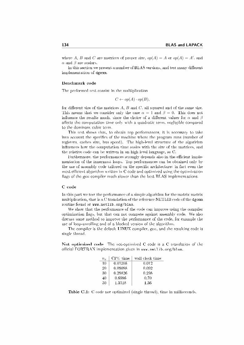
134 BLAS and LAPACK
where A, B and C are matrices of proper size, op(A) = A or op(A) = A′, andα and β are scalars.
In this section we present a number of BLAS versions, and test many di�erentimplementation of dgemm.
Benchmark code
The performed test consist in the multiplication
C ← op(A) · op(B),
for di�erent size of the matrices A, B and C, all squared and of the same size.This means that we consider only the case α = 1 and β = 0. This does notin�uence the results much, since the choice of a di�erent values for α and βa�ects the computation time only with a quadratic term, negligible comparedto the dominant cubic term.
This test shows that, to obtain top performances, it is necessary to takeinto account the speci�cs of the machine where the program runs (number ofregisters, caches size, bus speed). The high-level structure of the algorithmin�uences how the computation time scales with the size of the matrices, andthe relative code can be written in an high-level language, as C.
Furthermore, the performances strongly depends also in the e�cient imple-mentation of the innermost loops. Top performances can be obtained only bythe use of assembly code tailored on the speci�c architecture: in fact even themost e�cient algorithm written in C code and optimized using the optimization�ags of the gcc compiler much slower than the best BLAS implementations.
C code
In this part we test the performance of a simple algorithm for the matrix-matrixmultiplication, that is a C translation of the reference NETLIB code of the dgemmroutine found at www.netlib.org/blas.
We show that the performance of the code can improve using the compileroptimization �ags, but that can not compete against assembly code. We alsodiscuss some method to improve the performance of the code, for example theuse of loop-unrolling and of a blocked version of the algorithm.
The compiler is the default LINUX compiler, gcc, and the resulting code issingle thread.
Not optimized code The not-optimized C code is a C translation of theo�cial FORTRAN implementation given in www.netlib.org/blas.
nx CPU time wall clock time10 0.01208 0.01220 0.09088 0.09230 0.29826 0.29840 0.6986 0.7050 1.3518 1.36
Table C.1: C code not optimized (single thread), time in milliseconds.
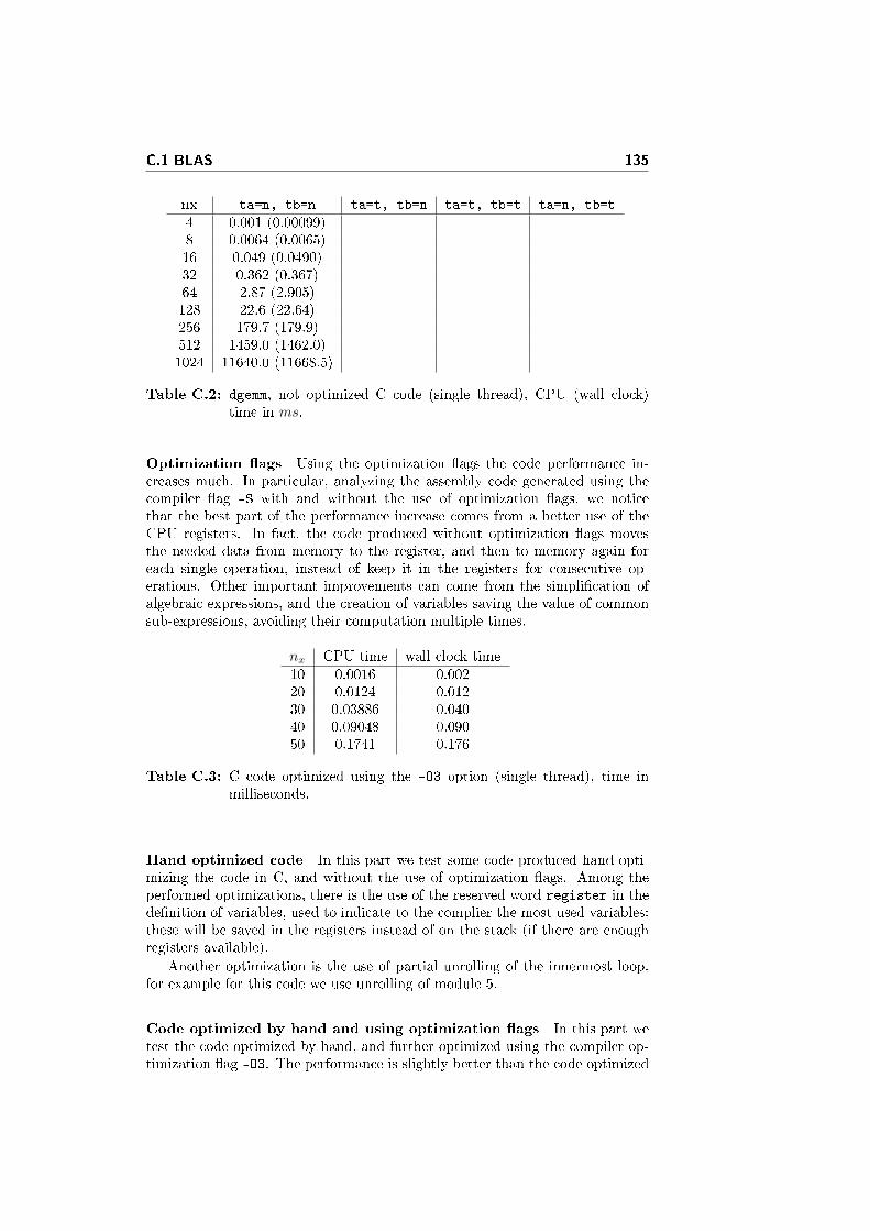
C.1 BLAS 135
nx ta=n, tb=n ta=t, tb=n ta=t, tb=t ta=n, tb=t
4 0.001 (0.00099)8 0.0064 (0.0065)16 0.049 (0.0490)32 0.362 (0.367)64 2.87 (2.905)128 22.6 (22.64)256 179.7 (179.9)512 1459.0 (1462.0)1024 11640.0 (11668.5)
Table C.2: dgemm, not optimized C code (single thread), CPU (wall clock)time in ms.
Optimization �ags Using the optimization �ags the code performance in-creases much. In particular, analyzing the assembly code generated using thecompiler �ag -S with and without the use of optimization �ags, we noticethat the best part of the performance increase comes from a better use of theCPU registers. In fact, the code produced without optimization �ags movesthe needed data from memory to the register, and then to memory again foreach single operation, instead of keep it in the registers for consecutive op-erations. Other important improvements can come from the simpli�cation ofalgebraic expressions, and the creation of variables saving the value of commonsub-expressions, avoiding their computation multiple times.
nx CPU time wall clock time10 0.0016 0.00220 0.0124 0.01230 0.03886 0.04040 0.09048 0.09050 0.1741 0.176
Table C.3: C code optimized using the -O3 option (single thread), time inmilliseconds.
Hand optimized code In this part we test some code produced hand opti-mizing the code in C, and without the use of optimization �ags. Among theperformed optimizations, there is the use of the reserved word register in thede�nition of variables, used to indicate to the complier the most used variables:these will be saved in the registers instead of on the stack (if there are enoughregisters available).
Another optimization is the use of partial unrolling of the innermost loop,for example for this code we use unrolling of module 5.
Code optimized by hand and using optimization �ags In this part wetest the code optimized by hand, and further optimized using the compiler op-timization �ag -O3. The performance is slightly better than the code optimized
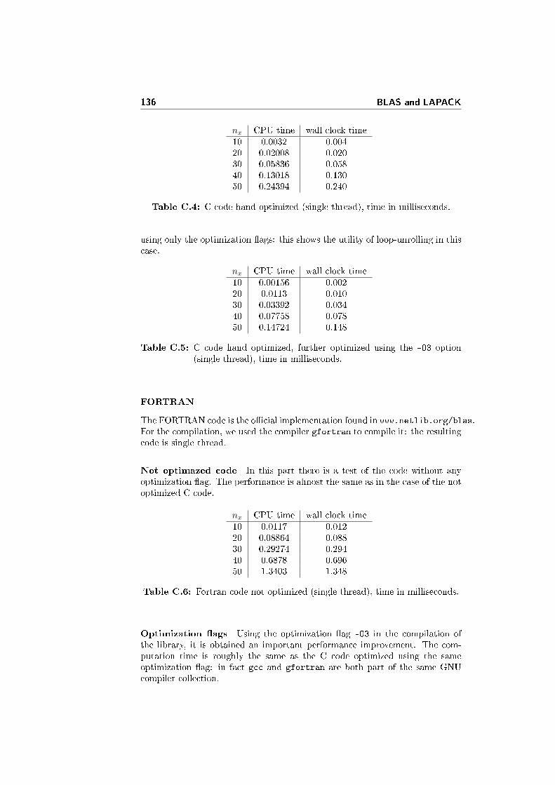
136 BLAS and LAPACK
nx CPU time wall clock time10 0.0032 0.00420 0.02008 0.02030 0.05836 0.05840 0.13018 0.13050 0.24394 0.240
Table C.4: C code hand optimized (single thread), time in milliseconds.
using only the optimization �ags: this shows the utility of loop-unrolling in thiscase.
nx CPU time wall clock time10 0.00156 0.00220 0.0113 0.01030 0.03392 0.03440 0.07758 0.07850 0.14724 0.148
Table C.5: C code hand optimized, further optimized using the -O3 option(single thread), time in milliseconds.
FORTRAN
The FORTRAN code is the o�cial implementation found in www.netlib.org/blas.For the compilation, we used the compiler gfortran to compile it: the resultingcode is single thread.
Not optimazed code In this part there is a test of the code without anyoptimization �ag. The performance is almost the same as in the case of the notoptimized C code.
nx CPU time wall clock time10 0.0117 0.01220 0.08864 0.08830 0.29274 0.29440 0.6878 0.69650 1.3403 1.348
Table C.6: Fortran code not optimized (single thread), time in milliseconds.
Optimization �ags Using the optimization �ag -O3 in the compilation ofthe library, it is obtained an important performance improvement. The com-putation time is roughly the same as the C code optimized using the sameoptimization �ag: in fact gcc and gfortran are both part of the same GNUcompiler collection.
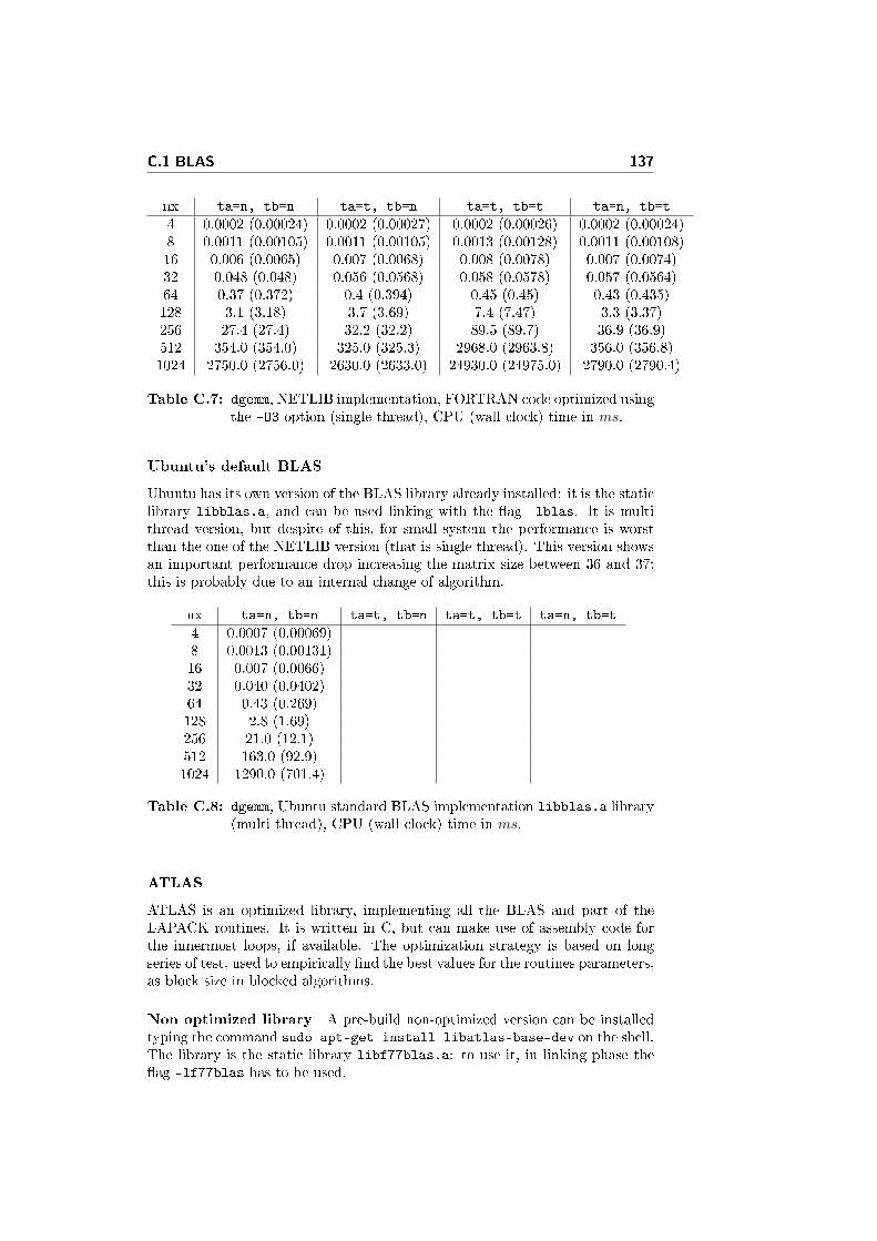
C.1 BLAS 137
nx ta=n, tb=n ta=t, tb=n ta=t, tb=t ta=n, tb=t
4 0.0002 (0.00024) 0.0002 (0.00027) 0.0002 (0.00026) 0.0002 (0.00024)8 0.0011 (0.00105) 0.0011 (0.00105) 0.0013 (0.00128) 0.0011 (0.00108)16 0.006 (0.0065) 0.007 (0.0068) 0.008 (0.0078) 0.007 (0.0074)32 0.048 (0.048) 0.056 (0.0568) 0.058 (0.0578) 0.057 (0.0564)64 0.37 (0.372) 0.4 (0.394) 0.45 (0.45) 0.43 (0.435)128 3.1 (3.18) 3.7 (3.69) 7.4 (7.47) 3.3 (3.37)256 27.4 (27.4) 32.2 (32.2) 89.5 (89.7) 36.9 (36.9)512 354.0 (354.0) 325.0 (325.3) 2968.0 (2963.8) 356.0 (356.8)1024 2750.0 (2756.0) 2630.0 (2633.0) 24930.0 (24975.0) 2790.0 (2790.4)
Table C.7: dgemm, NETLIB implementation, FORTRAN code optimized usingthe -O3 option (single thread), CPU (wall clock) time in ms.
Ubuntu's default BLAS
Ubuntu has its own version of the BLAS library already installed: it is the staticlibrary libblas.a, and can be used linking with the �ag -lblas. It is multithread version, but despite of this, for small system the performance is worstthan the one of the NETLIB version (that is single thread). This version showsan important performance drop increasing the matrix size between 36 and 37:this is probably due to an internal change of algorithm.
nx ta=n, tb=n ta=t, tb=n ta=t, tb=t ta=n, tb=t
4 0.0007 (0.00069)8 0.0013 (0.00131)16 0.007 (0.0066)32 0.040 (0.0402)64 0.43 (0.269)128 2.8 (1.69)256 21.0 (12.1)512 163.0 (92.9)1024 1290.0 (701.4)
Table C.8: dgemm, Ubuntu standard BLAS implementation libblas.a library(multi thread), CPU (wall clock) time in ms.
ATLAS
ATLAS is an optimized library, implementing all the BLAS and part of theLAPACK routines. It is written in C, but can make use of assembly code forthe innermost loops, if available. The optimization strategy is based on longseries of test, used to empirically �nd the best values for the routines parameters,as block size in blocked algorithms.
Non optimized library A pre-build non-optimized version can be installedtyping the command sudo apt-get install libatlas-base-dev on the shell.The library is the static library libf77blas.a: to use it, in linking phase the�ag -lf77blas has to be used.
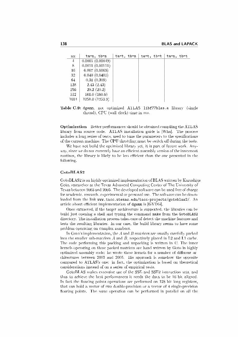
138 BLAS and LAPACK
nx ta=n, tb=n ta=t, tb=n ta=t, tb=t ta=n, tb=t
4 0.0005 (0.00049)8 0.0011 (0.00111)16 0.007 (0.0063)32 0.040 (0.0401)64 0.31 (0.309)128 2.43 (2.43)256 20.2 (20.2)512 161.0 (160.6)1024 1251.0 (1253.9)
Table C.9: dgemm, not optimized ATLAS libf77blas.a library (singlethread), CPU (wall clock) time in ms.
Optimization Better performances should be obtained compiling the ATLASlibrary from source code. ATLAS installation guide is [Wha]. The processincludes a long series of tests, used to tune the parameters to the speci�cationsof the current machine. The CPU throttling must be switch o� during the tests.
We have not build the optimized library yet, it is part of future work. Any-way, since we do not currently have an e�cient assembly version of the innermostroutines, the library is likely to be less e�cient than the one presented in thefollowing.
GotoBLAS2
GotoBLAS2 is an highly optimized implementation of BLAS written by KazushigeGoto, researcher at the Texas Advanced Computing Center of The University ofTexas between 2003 and 2005. The developed software can be used free of chargefor academic, research, experimental or personal use. The software can be down-loaded from the link www.tacc.utexas.edu/tacc-projects/gotoblas2/. Anarticle about e�cient implementation of dgemm is [GVDG].
Once extracted, if the target architecture is supported, the libraries can bebuild just opening a shell and typing the command make from the GotoBLAS2
directory. The installation process takes care of detect the machine features andtests the resulting libraries. In our case, the build library seems to have someproblem operating on complex numbers.
In Goto's implementation, the A and B matrices are usually carefully packedinto the smaller sub-matrices A and B, respectively placed in L2 and L1 cache.The code performing this packing and unpacking is written in C. The innerkernels operating on these packed matrices are hand written by Goto in highlyoptimized assembly code: he wrote these kernels for a number of di�erent ar-chitectures between 2003 and 2005. His approach is somehow the oppositecompared to ATLAS's one: in fact, the optimization is based on theoreticalconsiderations instead of on a series of empirical tests.
GotoBLAS makes extensive use of the SSE and SSE2 instruction sets, andthus to achieve the best performances it needs the data to be 16 bit aligned.In fact the �oating points operations are performed on 128 bit long registers,that can hold a vector of two double-precision or a vector of 4 single-precision�oating points. The same operation can be performed in parallel on all the
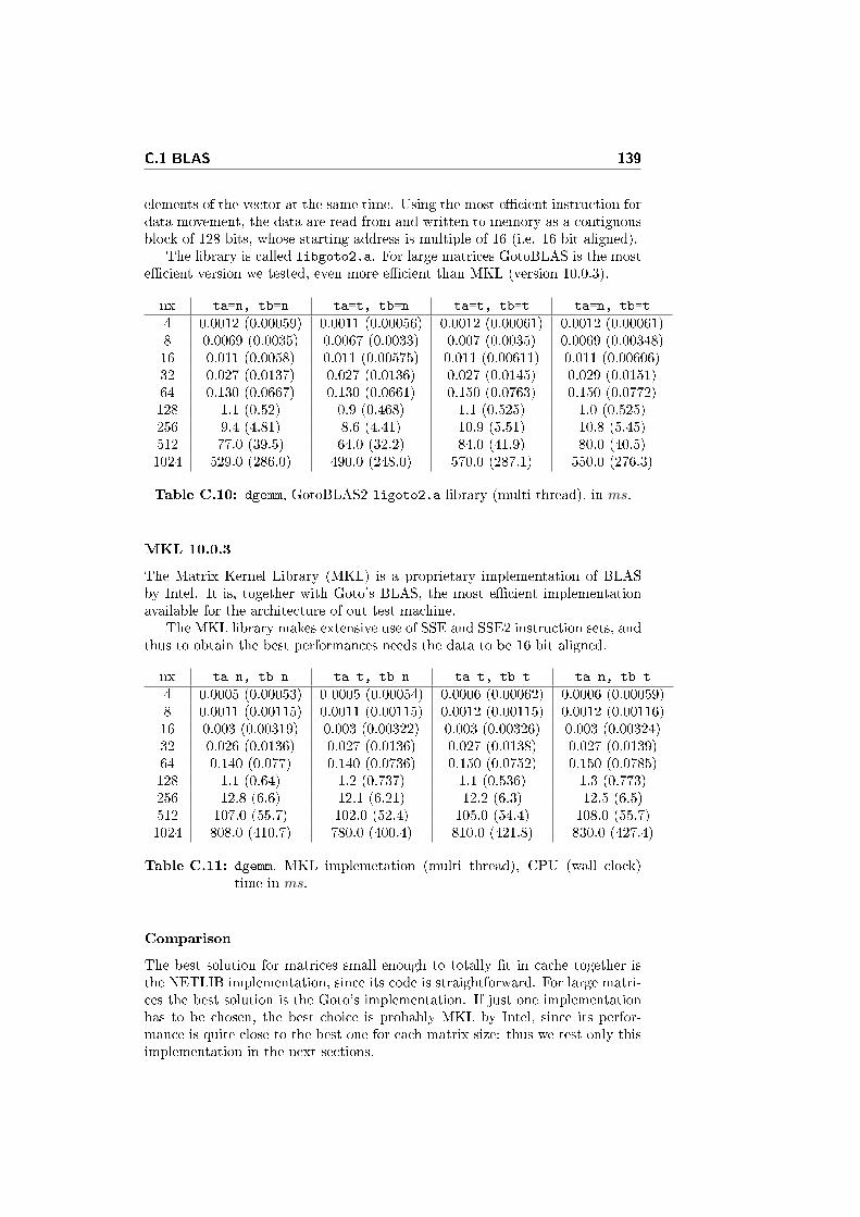
C.1 BLAS 139
elements of the vector at the same time. Using the most e�cient instruction fordata movement, the data are read from and written to memory as a contiguousblock of 128 bits, whose starting address is multiple of 16 (i.e. 16 bit aligned).
The library is called libgoto2.a. For large matrices GotoBLAS is the moste�cient version we tested, even more e�cient than MKL (version 10.0.3).
nx ta=n, tb=n ta=t, tb=n ta=t, tb=t ta=n, tb=t
4 0.0012 (0.00059) 0.0011 (0.00056) 0.0012 (0.00061) 0.0012 (0.00061)8 0.0069 (0.0035) 0.0067 (0.0033) 0.007 (0.0035) 0.0069 (0.00348)16 0.011 (0.0058) 0.011 (0.00575) 0.011 (0.00611) 0.011 (0.00606)32 0.027 (0.0137) 0.027 (0.0136) 0.027 (0.0145) 0.029 (0.0151)64 0.130 (0.0667) 0.130 (0.0661) 0.150 (0.0763) 0.150 (0.0772)128 1.1 (0.52) 0.9 (0.468) 1.1 (0.525) 1.0 (0.525)256 9.4 (4.81) 8.6 (4.41) 10.9 (5.51) 10.8 (5.45)512 77.0 (39.5) 64.0 (32.2) 84.0 (41.9) 80.0 (40.5)1024 529.0 (286.0) 490.0 (248.0) 570.0 (287.1) 550.0 (276.3)
Table C.10: dgemm, GotoBLAS2 ligoto2.a library (multi thread), in ms.
MKL 10.0.3
The Matrix Kernel Library (MKL) is a proprietary implementation of BLASby Intel. It is, together with Goto's BLAS, the most e�cient implementationavailable for the architecture of out test machine.
The MKL library makes extensive use of SSE and SSE2 instruction sets, andthus to obtain the best performances needs the data to be 16 bit aligned.
nx ta=n, tb=n ta=t, tb=n ta=t, tb=t ta=n, tb=t
4 0.0005 (0.00053) 0 0005 (0.00054) 0.0006 (0.00062) 0.0006 (0.00059)8 0.0011 (0.00115) 0.0011 (0.00115) 0.0012 (0.00115) 0.0012 (0.00116)16 0.003 (0.00319) 0.003 (0.00322) 0.003 (0.00326) 0.003 (0.00324)32 0.026 (0.0136) 0.027 (0.0136) 0.027 (0.0138) 0.027 (0.0139)64 0.140 (0.077) 0.140 (0.0736) 0.150 (0.0752) 0.150 (0.0785)128 1.1 (0.64) 1.2 (0.737) 1.1 (0.536) 1.3 (0.773)256 12.8 (6.6) 12.1 (6.21) 12.2 (6.3) 12.5 (6.5)512 107.0 (55.7) 102.0 (52.4) 105.0 (54.4) 108.0 (55.7)1024 808.0 (410.7) 780.0 (400.4) 810.0 (421.8) 830.0 (427.4)
Table C.11: dgemm, MKL implemetation (multi thread), CPU (wall clock)time in ms.
Comparison
The best solution for matrices small enough to totally �t in cache together isthe NETLIB implementation, since its code is straightforward. For large matri-ces the best solution is the Goto's implementation. If just one implementationhas to be chosen, the best choice is probably MKL by Intel, since its perfor-mance is quite close to the best one for each matrix size: thus we test only thisimplementation in the next sections.
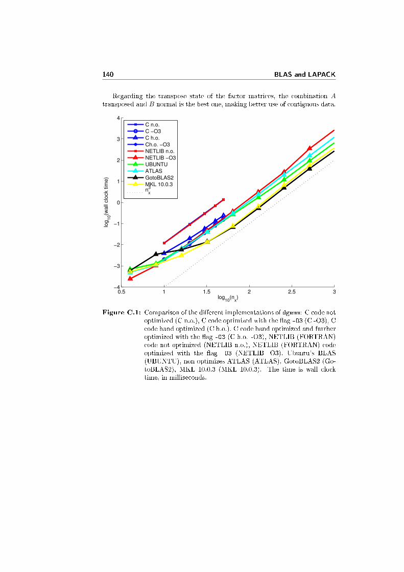
140 BLAS and LAPACK
Regarding the transpose state of the factor matrices, the combination Atransposed and B normal is the best one, making better use of contiguous data.
0.5 1 1.5 2 2.5 3−4
−3
−2
−1
0
1
2
3
4
log10
(nx)
log
10(w
all
clo
ck t
ime
)
C n.o.
C −O3
C h.o.
Ch.o. −O3
NETLIB n.o.
NETLIB −O3
UBUNTU
ATLAS
GotoBLAS2
MKL 10.0.3n
x
3
Figure C.1: Comparison of the di�erent implementations of dgemm: C code notoptimized (C n.o.), C code optimized with the �ag -O3 (C -O3), Ccode hand optimized (C h.o.), C code hand optimized and furtheroptimized with the �ag -O3 (C h.o. -O3), NETLIB (FORTRAN)code not optimized (NETLIB n.o.), NETLIB (FORTRAN) codeoptimized with the �ag -O3 (NETLIB -O3), Ubuntu's BLAS(UBUNTU), non optimizes ATLAS (ATLAS), GotoBLAS2 (Go-toBLAS2), MKL 10.0.3 (MKL 10.0.3). The time is wall clocktime, in milliseconds.
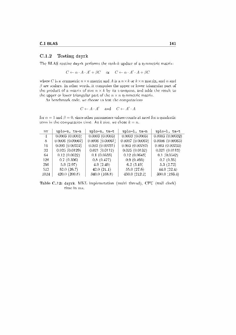
C.1 BLAS 141
C.1.2 Testing dsyrk
The BLAS routine dsyrk performs the rank-k update of a symmetric matrix:
C ← α ·A ·A′ + βC or C ← α ·A′ ·A+ βC
where C is a symmetric n×n matrix and A is a n×k or k×n matrix, and α andβ are scalars. In other words, it computes the upper or lower triangular part ofthe product of a matrix of size n × k by its transpose, and adds the result tothe upper or lower triangular part of the n× n symmetric matrix.
As benchmark code, we choose to test the computations
C ← A ·A′ and C ← A′ ·A
for α = 1 and β = 0, since other parameters values counts at most for a quadraticterm in the computation time. As k size, we chose k = n.
nx uplo=u, ta=n uplo=u, ta=t uplo=l, ta=n uplo=l, ta=t
4 0.0003 (0.0003) 0.0003 (0.0003) 0.0003 (0.0003) 0.0003 (0.00032)8 0.0006 (0.00062) 0.0006 (0.00061) 0.0007 (0.00062) 0.0006 (0.00063)16 0.003 (0.00252) 0.002 (0.00231) 0.003 (0.00282) 0.003 (0.00233)32 0.025 (0.0129) 0.021 (0.0112) 0.025 (0.0132) 0.021 (0.0113)64 0.12 (0.0622) 0.1 (0.0533) 0.12 (0.0643) 0.1 (0.0542)128 0.7 (0.396) 0.8 (0.477) 0.9 (0.493) 0.7 (0.35)256 5.9 (2.97) 4.9 (2.49) 6.2 (3.19) 5.3 (2.72)512 52.0 (26.7) 42.0 (21.1) 55.0 (27.6) 44.0 (22.4)1024 420.0 (209.8) 340.0 (168.8) 430.0 (212.2) 390.0 (193.4)
Table C.12: dsyrk, MKL implemetation (multi thread), CPU (wall clock)time in ms.
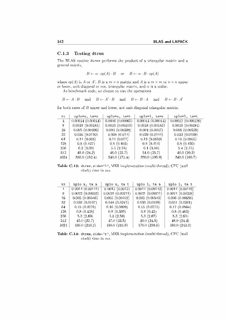
142 BLAS and LAPACK
C.1.3 Testing dtrmm
The BLAS routine dtrmm performs the product of a triangular matrix and ageneral matrix,
B ← α · op(A) ·B or B ← α ·B · op(A)
where op(A) is A or A′, B is a m× n matrix and A is a m×m or n× n upperor lower, unit diagonal or not, triangular matrix, and α is a scalar.
As benchmark code, we choose to test the operations
B ← A ·B and B ← A′ ·B and B ← B ·A and B ← B ·A′
for both cases of B upper and lower, not unit diagonal triangular matrix.
nx uplo=u, ta=n uplo=u, ta=t uplo=l, ta=n uplo=l, ta=t
4 0.00014 (0.00014) 0.0006 (0.00065) 0.00014 (0.00014) 0.00012 (0.000126)8 0.0018 (0.00185) 0.0010 (0.00103) 0.0018 (0.00185) 0.0019 (0.00194)16 0.005 (0.00496) 0.004 (0.00398) 0.004 (0.0047) 0.006 (0.00559)32 0.030 (0.0150) 0.028 (0.014) 0.029 (0.0144) 0.033 (0.0169)64 0.14 (0.068) 0.14 (0.071) 0.13 (0.0659) 0.16 (0.0805)128 0.8 (0.427) 0.8 (0.403) 0.8 (0.414) 0.8 (0.430)256 6.2 (3.09) 5.5 (2.78) 6.1 (3.08) 5.4 (2.75)512 49.0 (24.2) 46.0 (22.7) 51.0 (25.7) 40.0 (20.2)1024 380.0 (192.4) 340.0 (171.4) 390.0 (193.9) 340.0 (169.7)
Table C.13: dtrmm, side='l', MKL implemetation (multi thread), CPU (wallclock) time in ms.
nx uplo=u, ta=n uplo=u, ta=t uplo=l, ta=n uplo=l, ta=t
4 0 0014 (0.00141) 0 0015 (0.0015) 0.0014 (0.00143) 0.0014 (0.00143)8 0.0023 (0.00233) 0.0021 (0.00211) 0.0021 (0.00211) 0.0024 (0.00238)16 0.005 (0.00546) 0.005 (0.00459) 0.005 (0.00542) 0.006 (0.00638)32 0.039 (0.0197) 0.048 (0.0241) 0.039 (0.0199) 0.051 (0.0261)64 0.15 (0.0776) 0.16 (0.0809) 0.15 (0.0775) 0.17 (0.0864)128 0.8 (0.428) 0.8 (0.399) 0.8 (0.42) 0.8 (0.403)256 5.3 (2.69) 5.1 (2.59) 5.3 (2.67) 5.3 (2.65)512 45.0 (22.7) 47.0 (23.5) 49.0 (24.5) 48.0 (24.4)1024 480.0 (240.2) 480.0 (244.8) 470.0 (238.6) 480.0 (243.3)
Table C.14: dtrmm, side='r', MKL implemetation (multi thread), CPU (wallclock) time in ms.
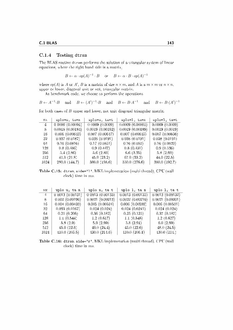
C.1 BLAS 143
C.1.4 Testing dtrsm
The BLAS routine dtrsm performs the solution of a triangular system of linearequations, where the right hand side is a matrix,
B ← α · op(A)−1 ·B or B ← α ·B · op(A)−1
where op(A) is A or A′, B is a matrix of size n×m, and A is a m×m or n×n,upper or lower, diagonal unit or not, triangular matrix.
As benchmark code, we choose to perform the operations
B ← A−1·B and B ← (A′)−1·B and B ← B·A−1 and B ← B·(A′)−1
for both cases of B upper and lower, not unit diagonal triangular matrix.
nx uplo=u, ta=n uplo=u, ta=t uplo=l, ta=n uplo=l, ta=t
4 0 0009 (0.00091) 0 0009 (0.0009) 0.0009 (0.00091) 0.0009 (0.0009)8 0.0018 (0.00184) 0.0019 (0.00192) 0.0019 (0.00189) 0.0019 (0.0019)16 0.006 (0.00643) 0.007 (0.00647) 0.007 (0.00645) 0.007 (0.00656)32 0.037 (0.0187) 0.038 (0.0191) 0.038 (0.0191) 0.038 (0.0191)64 0.16 (0.0816) 0.17 (0.0851) 0.16 (0.082) 0.16 (0.0829)128 0.8 (0.486) 0.9 (0.447) 0.8 (0.431) 0.9 (0.536)256 5.4 (2.86) 5.6 (2.89) 6.6 (3.35) 5.8 (2.93)512 41.0 (21.8) 45.0 (23.2) 67.0 (33.2) 44.0 (22.5)1024 280.0 (144.7) 380.0 (198.6) 550.0 (276.6) 380.0 (192.7)
Table C.15: dtrsm, side='l', MKL implemetation (multi thread), CPU (wallclock) time in ms.
nx uplo=u, ta=n uplo=u, ta=t uplo=l, ta=n uplo=l, ta=t
4 0 0013 (0.00131) 0 0013 (0.00133) 0.0013 (0.00135) 0.0013 (0.00132)8 0.002 (0.00196) 0.0021 (0.00213) 0.0022 (0.00216) 0.0021 (0.00201)16 0.004 (0.00439) 0.005 (0.00524) 0.006 (0.00592) 0.006 (0.00531)32 0.033 (0.0167) 0.024 (0.024) 0.024 (0.0241) 0.024 (0.024)64 0.21 (0.206) 0.36 (0.182) 0.25 (0.125) 0.37 (0.187)128 1.1 (0.544) 1.2 (0.617) 1.1 (0.548) 1.2 (0.627)256 5.8 (2.9) 5.9 (2.99) 5.8 (2.91) 6.0 (2.99)512 45.0 (22.6) 49.0 (24.4) 45.0 (22.6) 48.0 (24.5)1024 410.0 (205.5) 430.0 (214.6) 410.0 (206.1) 430.0 (214.)
Table C.16: dtrsm, side='r', MKL implemetation (multi thread), CPU (wallclock) time in ms.
144 BLAS and LAPACK
C.2 LAPACK
LAPACK is a library containing a number of routines for linear algebra prob-lems, such as matrix factorizations, solution of linear systems and linear leastsquares, eigenvalue problems and singular value decomposition. The code iscurrently written in Fortran 90.
LAPACK depends upon BLAS to perform the basic linear algebra opera-tions, such as matrix-matrix and matrix-vector multiplication: LAPACK per-formance thus strongly depends on the BLAS library it links against. LAPACK'sroutines are iterative algorithms, and usually there are two versions for each al-gorithm, an unblocked one (using the level 2 BLAS) and a blocked one (usingthe level 3 BLAS and the unblocked version as subroutine).
We teste a number of versions of the LAPACK library, using pre-built li-braries or compiling from the source code, linking against di�erent BLAS li-braries.
By downloading ATLAS, we also download a pre-build sub-set of the LA-PACK library linking against libf77blas.a. Another possibility is the instal-lation of Ubuntu's default LAPACK, linking against libblas.a.
It is also possible to compile from source code, and choose the BLAS li-brary to link against. The source code can be downloaded from the web-site www.netlib.org/lapack, in the compressed �le lapack-3.4.0.tgz (thecurrent latest version in 3.4.0). After extraction, we have to enter into thejust created folder lapack-3.4.0, and rename the �le make.inc.example intomake.inc (it is an example �le to install LAPACK on Linux). Then we haveto edit the �le make.inc, writing in the row BLASLIB the path of the BLASlibrary we want LAPACK to link against.1 After this, the library can be buildby opening a shell, entering in the folder lapack-3.4.0 and typing the com-mand make all (this is building the library and testing the BLAS and LAPACKimplementations).
This produces a library called liblapack.a: it is possible to move the librarywhere we want to place it. In order to use it, in linking phase we need to linkour programs against the LAPACK library, the BLAS library and the gfortranlibrary (with the command -lgfortran), written in this order.
We decided to test 4 LAPACK implementations: the pre-build Ubuntu'sLAPACK, the pre-build ATLAS LAPACK, the compiled library linking againstthe standard FORTRAN BLAS and the compiled library linking against theMKL BLAS; for some routines we are also writing a recursive version.
C.2.1 Testing dpotrf
In this section we test di�erent implementation of Cholesky factorization. Wetest the algorithm based on the 2× 2 and 3× 3 blocks matrix, in both iterativeblocked and recursive versions (the LAPACK routine dpotrf is the iterativeversion of the algorithm based on the 3 × 3 blocks matrix) and the LAPACKroutine dpotf2 (an unblocked version of the algorithm based on the 3×3 blocksmatrix).
Regarding the recursive algorithms, as base cases are use routines directlyfactorizing matrices of size 1× 1, 2× 2, 3× 3 and 4× 4, or the dpotf2 routine.
1It is possible to customize many other options, like the compiler (the default is gfortran)and the optimization level (the default is O2).
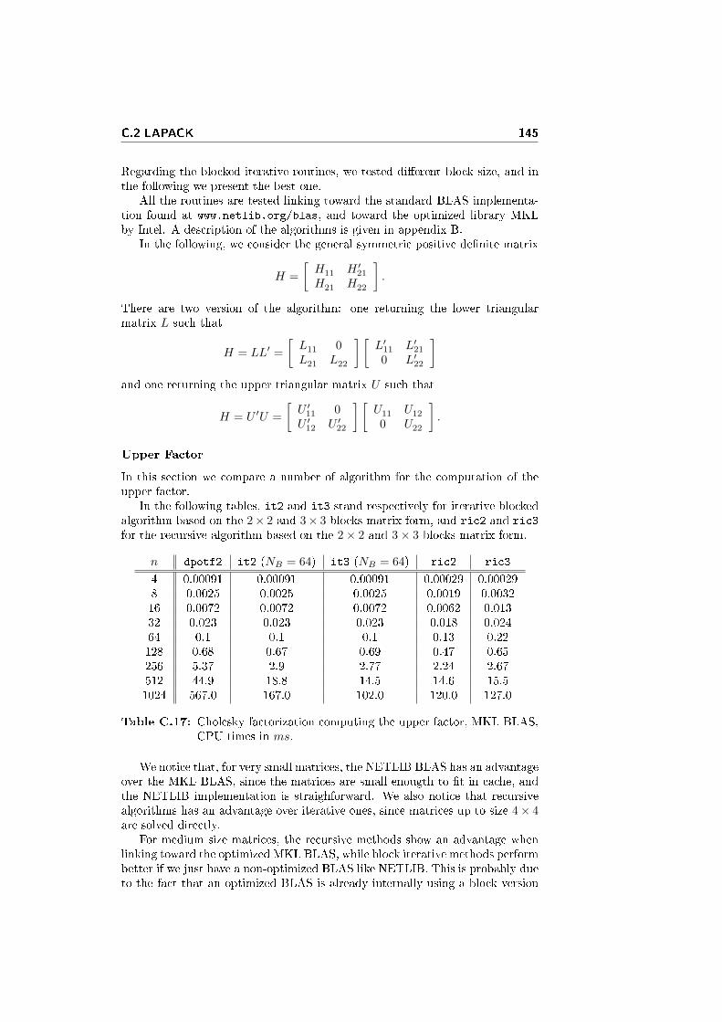
C.2 LAPACK 145
Regarding the blocked iterative routines, we tested di�erent block size, and inthe following we present the best one.
All the routines are tested linking toward the standard BLAS implementa-tion found at www.netlib.org/blas, and toward the optimized library MKLby Intel. A description of the algorithms is given in appendix B.
In the following, we consider the general symmetric positive de�nite matrix
H =
[H11 H ′21
H21 H22
].
There are two version of the algorithm: one returning the lower triangularmatrix L such that
H = LL′ =
[L11 0L21 L22
] [L′11 L′21
0 L′22
]and one returning the upper triangular matrix U such that
H = U ′U =
[U ′11 0U ′12 U ′22
] [U11 U12
0 U22
].
Upper Factor
In this section we compare a number of algorithm for the computation of theupper factor.
In the following tables, it2 and it3 stand respectively for iterative blockedalgorithm based on the 2× 2 and 3× 3 blocks matrix form, and ric2 and ric3
for the recursive algorithm based on the 2× 2 and 3× 3 blocks matrix form.
n dpotf2 it2 (NB = 64) it3 (NB = 64) ric2 ric3
4 0.00091 0.00091 0.00091 0.00029 0.000298 0.0025 0.0025 0.0025 0.0019 0.003216 0.0072 0.0072 0.0072 0.0062 0.01332 0.023 0.023 0.023 0.018 0.02464 0.1 0.1 0.1 0.13 0.22128 0.68 0.67 0.69 0.47 0.65256 5.37 2.9 2.77 2.24 2.67512 44.9 18.8 14.5 14.6 15.51024 567.0 167.0 102.0 120.0 127.0
Table C.17: Cholesky factorization computing the upper factor, MKL BLAS,CPU times in ms.
We notice that, for very small matrices, the NETLIB BLAS has an advantageover the MKL BLAS, since the matrices are small enougth to �t in cache, andthe NETLIB implementation is straighforward. We also notice that recursivealgorithms has an advantage over iterative ones, since matrices up to size 4× 4are solved directly.
For medium size matrices, the recursive methods show an advantage whenlinking toward the optimized MKL BLAS, while block iterative methods performbetter if we just have a non-optimized BLAS like NETLIB. This is probably dueto the fact that an optimized BLAS is already internally using a block version
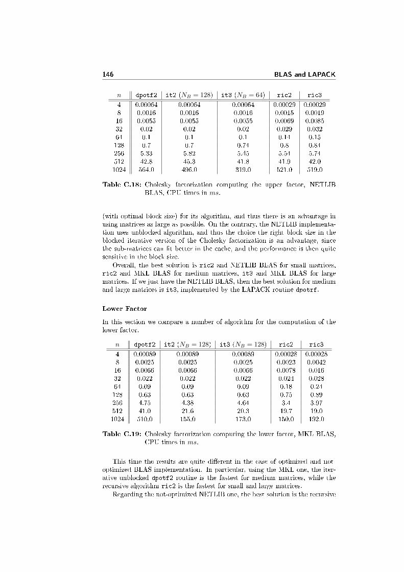
146 BLAS and LAPACK
n dpotf2 it2 (NB = 128) it3 (NB = 64) ric2 ric3
4 0.00064 0.00064 0.00064 0.00029 0.000298 0.0016 0.0016 0.0016 0.0015 0.001916 0.0055 0.0055 0.0055 0.0069 0.008532 0.02 0.02 0.02 0.029 0.03264 0.1 0.1 0.1 0.14 0.15128 0.7 0.7 0.74 0.8 0.84256 5.33 5.82 5.45 5.54 5.74512 42.8 45.3 41.8 41.9 42.01024 564.0 496.0 319.0 521.0 519.0
Table C.18: Cholesky factorization computing the upper factor, NETLIBBLAS, CPU times in ms.
(with optimal block size) for its algorithm, and thus there is an advantage inusing matrices as large as possible. On the contrary, the NETLIB implementa-tion uses unblocked algorithm, and thus the choice the right block size in theblocked iterative version of the Cholesky factorization is an advantage, sincethe sub-matrices can �t better in the cache, and the performance is then quitesensitive in the block size.
Overall, the best solution is ric2 and NETLIB BLAS for small matrices,ric2 and MKL BLAS for medium matrices, it3 and MKL BLAS for largematrices. If we just have the NETLIB BLAS, then the best solution for mediumand large matrices is it3, implemented by the LAPACK routine dpotrf.
Lower Factor
In this section we compare a number of algorithm for the computation of thelower factor.
n dpotf2 it2 (NB = 128) it3 (NB = 128) ric2 ric3
4 0.00089 0.00089 0.00089 0.00028 0.000288 0.0025 0.0025 0.0025 0.0023 0.004216 0.0066 0.0066 0.0066 0.0078 0.01632 0.022 0.022 0.022 0.024 0.02864 0.09 0.09 0.09 0.18 0.24128 0.63 0.63 0.63 0.75 0.89256 4.75 4.38 4.64 3.4 3.97512 41.0 21.6 20.3 19.7 19.01024 510.0 155.0 173.0 150.0 192.0
Table C.19: Cholesky factorization computing the lower factor, MKL BLAS,CPU times in ms.
This time the results are quite di�erent in the case of optimized and not-optimized BLAS implementation. In particular, using the MKL one, the iter-ative unblocked dpotf2 routine is the fastest for medium matrices, while therecursive algorithm ric2 is the fastest for small and large matrices.
Regarding the not-optimized NETLIB one, the best solution is the recursive
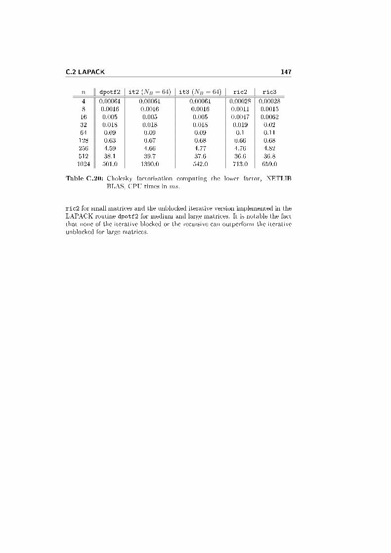
C.2 LAPACK 147
n dpotf2 it2 (NB = 64) it3 (NB = 64) ric2 ric3
4 0.00061 0.00061 0.00061 0.00028 0.000288 0.0016 0.0016 0.0016 0.0011 0.001516 0.005 0.005 0.005 0.0047 0.006232 0.018 0.018 0.018 0.019 0.0264 0.09 0.09 0.09 0.1 0.11128 0.63 0.67 0.68 0.66 0.68256 4.59 4.66 4.77 4.76 4.82512 38.1 39.7 37.6 36.6 36.81024 501.0 1390.0 542.0 713.0 659.0
Table C.20: Cholesky factorization computing the lower factor, NETLIBBLAS, CPU times in ms.
ric2 for small matrices and the unblocked iterative version implemented in theLAPACK routine dpotf2 for medium and large matrices. It is notable the factthat none of the iterative blocked or the recursive can outperform the iterativeunblocked for large matrices.

148 BLAS and LAPACK
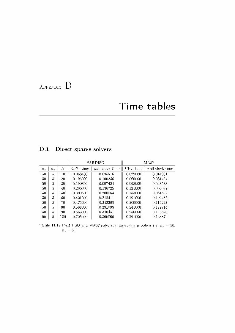
Appendix D
Time tables
D.1 Direct sparse solvers
PARDISO MA57
nx nu N CPU time wall clock time CPU time wall clock time
50 5 10 0.068400 0.035516 0.029000 0.01499150 5 20 0.196000 0.100256 0.060000 0.03146750 5 30 0.190800 0.097424 0.093000 0.04853850 5 40 0.266000 0.136725 0.121000 0.06469250 5 50 0.390500 0.200064 0.153000 0.08159250 5 60 0.421000 0.215411 0.191000 0.10248550 5 70 0.475000 0.243368 0.209000 0.11424750 5 80 0.568000 0.291098 0.241000 0.12971450 5 90 0.663000 0.340451 0.256000 0.14682650 5 100 0.705000 0.360866 0.291000 0.163874
Table D.1: PARDISO and MA57 solvers, mass-spring problem 7.2, nx = 50,nu = 5.
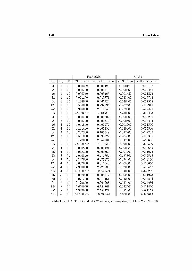
150 Time tables
PARDISO MA57
nx nu N CPU time wall clock time CPU time wall clock time
4 1 10 0.000358 0.000183 0.000170 0.0001928 1 10 0.000700 0.000373 0.000460 0.00046116 1 10 0.006750 0.003466 0.001550 0.00157232 1 10 0.021100 0.010771 0.013500 0.01374264 1 10 0.128600 0.065823 0.046000 0.027568128 1 10 0.586000 0.299835 0.202500 0.108911256 1 10 3.916000 2.016855 0.979000 0.599491512 1 10 33.930000 17.404348 7.730000 4.3624934 2 10 0.000400 0.000204 0.000200 0.0002068 2 10 0.000720 0.000372 0.000500 0.00049416 2 10 0.001800 0.000972 0.001500 0.00150032 2 10 0.131400 0.067259 0.010300 0.00532664 2 10 0.207800 0.106349 0.042200 0.022207128 2 10 0.581000 0.297627 0.205000 0.108307256 2 10 5.178000 2.652331 1.017000 0.580696512 2 10 27.420000 14.078512 7.690000 4.3385598 4 10 0.000800 0.000421 0.000580 0.00065516 4 10 0.018300 0.009364 0.001700 0.00167532 4 10 0.026800 0.013769 0.011100 0.00583564 4 10 0.147600 0.075676 0.044200 0.023166128 4 10 0.607000 0.311040 0.205000 0.110650256 4 10 4.350000 2.229680 1.020000 0.580832512 4 10 38.320000 19.640594 7.640000 4.34220016 8 10 0.008200 0.004212 0.002000 0.00197332 8 10 0.021700 0.011161 0.012500 0.00654464 8 10 0.129800 0.066668 0.047400 0.024536128 8 10 0.690000 0.354867 0.212000 0.111890256 8 10 5.343000 2.750471 1.021000 0.591158512 8 10 31.790000 16.393541 7.700000 4.395613
Table D.2: PARDISO and MA57 solvers, mass-spring problem 7.2, N = 10.
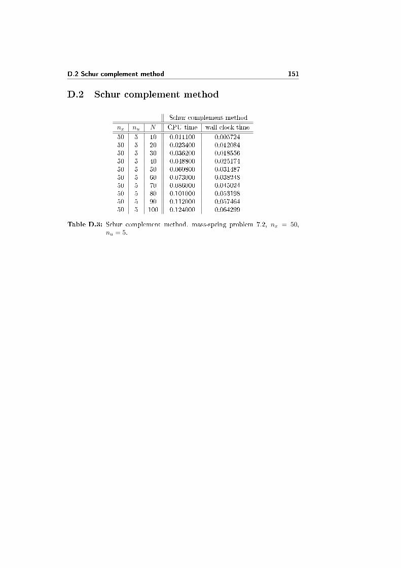
D.2 Schur complement method 151
D.2 Schur complement method
Schur complement method
nx nu N CPU time wall clock time
50 5 10 0.011100 0.00572450 5 20 0.023400 0.01208450 5 30 0.036200 0.01855650 5 40 0.048800 0.02517450 5 50 0.060800 0.03148750 5 60 0.073000 0.03824850 5 70 0.086000 0.04502450 5 80 0.101000 0.05319850 5 90 0.112000 0.05746450 5 100 0.124000 0.064299
Table D.3: Schur complement method, mass-spring problem 7.2, nx = 50,nu = 5.
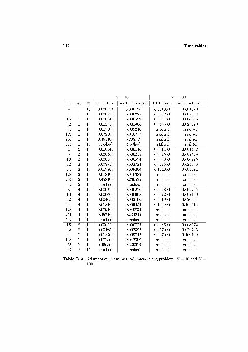
152 Time tables
N = 10 N = 100
nx nu N CPU time wall clock time CPU time wall clock time
4 1 10 0.000134 0.000136 0.001300 0.0013208 1 10 0.000230 0.000225 0.002200 0.00230816 1 10 0.000540 0.000539 0.006400 0.00628532 1 10 0.003750 0.001966 0.046500 0.02327064 1 10 0.017500 0.009240 crashed crashed128 1 10 0.079100 0.040777 crashed crashed256 1 10 0.461400 0.238059 crashed crashed512 1 10 crashed crashed crashed crashed4 2 10 0.000144 0.000146 0.001400 0.0014028 2 10 0.000260 0.000255 0.002500 0.00254916 2 10 0.000580 0.000574 0.006800 0.00672532 2 10 0.003950 0.002024 0.047500 0.02530964 2 10 0.017800 0.009206 0.194000 0.099484128 2 10 0.078400 0.040389 crashed crashed256 2 10 0.458400 0.236535 crashed crashed512 2 10 crashed crashed crashed crashed8 4 10 0.000270 0.000270 0.002800 0.00276516 4 10 0.000600 0.000608 0.007200 0.00719632 4 10 0.004050 0.002100 0.051000 0.02606464 4 10 0.018400 0.009454 0.196000 0.103613128 4 10 0.079500 0.040824 crashed crashed256 4 10 0.457400 0.234945 crashed crashed512 4 10 crashed crashed crashed crashed16 8 10 0.000720 0.000725 0.008600 0.00867232 8 10 0.004650 0.002392 0.057000 0.02979564 8 10 0.018900 0.009742 0.207000 0.106149128 8 10 0.081800 0.042090 crashed crashed256 8 10 0.466800 0.239919 crashed crashed512 8 10 crashed crashed crashed crashed
Table D.4: Schur complement method, mass-spring problem, N = 10 andN =100.
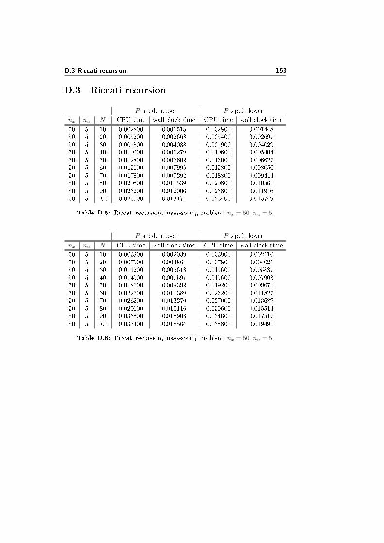
D.3 Riccati recursion 153
D.3 Riccati recursion
P s.p.d. upper P s.p.d. lower
nx nu N CPU time wall clock time CPU time wall clock time
50 5 10 0.002800 0.001513 0.002800 0.00144850 5 20 0.005200 0.002663 0.005400 0.00269750 5 30 0.007800 0.004038 0.007900 0.00402950 5 40 0.010200 0.005279 0.010600 0.00540450 5 50 0.012800 0.006602 0.013000 0.00662750 5 60 0.015600 0.007995 0.015800 0.00805050 5 70 0.017800 0.009292 0.018800 0.00944450 5 80 0.020600 0.010539 0.020800 0.01056150 5 90 0.023200 0.012006 0.023800 0.01194650 5 100 0.025600 0.013174 0.026400 0.013749
Table D.5: Riccati recursion, mass-spring problem, nx = 50, nu = 5.
P s.p.d. upper P s.p.d. lower
nx nu N CPU time wall clock time CPU time wall clock time
50 5 10 0.003900 0.002039 0.003900 0.00211050 5 20 0.007600 0.003864 0.007800 0.00402150 5 30 0.011200 0.005618 0.011600 0.00583750 5 40 0.014900 0.007597 0.015600 0.00790350 5 50 0.018600 0.009392 0.019200 0.00967150 5 60 0.022600 0.011389 0.023200 0.01182750 5 70 0.026200 0.013270 0.027000 0.01368950 5 80 0.029600 0.015116 0.030600 0.01551450 5 90 0.033600 0.016908 0.034600 0.01751750 5 100 0.037400 0.018864 0.038800 0.019491
Table D.6: Riccati recursion, mass-spring problem, nx = 50, nu = 5.
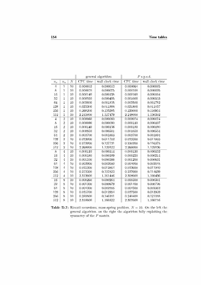
154 Time tables
general algorithm P s.p.s.d.
nx nu N CPU time wall clock time CPU time wall clock time
4 1 10 0.000052 0.000052 0.000064 0.0000658 1 10 0.000070 0.000075 0.000100 0.00009516 1 10 0.000140 0.000138 0.000160 0.00016432 1 10 0.000950 0.000495 0.001000 0.00055364 1 10 0.003600 0.001855 0.003500 0.001782128 1 10 0.023300 0.011888 0.021800 0.011037256 1 10 0.268200 0.135285 0.220000 0.110954512 1 10 2.245000 1.127479 2.248000 1.1303024 2 10 0.000060 0.000060 0.000074 0.0000748 2 10 0.000090 0.000090 0.000110 0.00010716 2 10 0.000140 0.000156 0.000180 0.00018032 2 10 0.000950 0.000501 0.001050 0.00055464 2 10 0.003700 0.001863 0.003700 0.001894128 2 10 0.023000 0.011702 0.023300 0.011803256 2 10 0.272000 0.137731 0.230200 0.116378512 2 10 2.268000 1.139122 2.266000 1.1391368 4 10 0.000110 0.000114 0.000130 0.00013216 4 10 0.000180 0.000189 0.000220 0.00021432 4 10 0.001100 0.000566 0.001200 0.00063164 4 10 0.003900 0.002000 0.004000 0.002048128 4 10 0.025300 0.012864 0.023600 0.011940256 4 10 0.273200 0.137822 0.227000 0.114639512 4 10 2.313000 1.161446 2.308000 1.16043616 8 10 0.000260 0.000264 0.000300 0.00030132 8 10 0.001300 0.000679 0.001400 0.00072664 8 10 0.004300 0.002208 0.004500 0.002362128 8 10 0.025700 0.012994 0.027500 0.013959256 8 10 0.289800 0.146181 0.240400 0.121188512 8 10 2.310000 1.160322 2.307000 1.160716
Table D.7: Riccati recursions, mass-spring problem, N = 10. On the left thegeneral algorithm, on the right the algorithm fully exploiting thesymmetry of the P matrix.
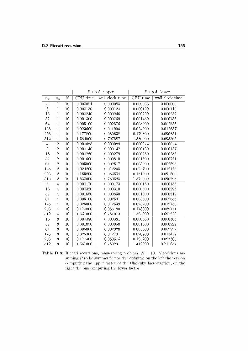
D.3 Riccati recursion 155
P s.p.d. upper P s.p.d. lower
nx nu N CPU time wall clock time CPU time wall clock time
4 1 10 0.000084 0.000085 0.000066 0.0000668 1 10 0.000130 0.000124 0.000120 0.00011616 1 10 0.000240 0.000246 0.000220 0.00023232 1 10 0.001500 0.000769 0.001450 0.00078664 1 10 0.005100 0.002576 0.005000 0.002536128 1 10 0.023600 0.011994 0.024900 0.012637256 1 10 0.177800 0.089638 0.179800 0.090851512 1 10 1.584000 0.797587 1.380000 0.6953654 2 10 0.000088 0.000089 0.000074 0.0000748 2 10 0.000140 0.000142 0.000130 0.00013716 2 10 0.000280 0.000279 0.000260 0.00025832 2 10 0.001600 0.000810 0.001500 0.00077164 2 10 0.005000 0.002617 0.005000 0.002593128 2 10 0.024200 0.012265 0.024700 0.012476256 2 10 0.165800 0.083604 0.181600 0.091560512 2 10 1.550000 0.780625 1.372000 0.6962988 4 10 0.000170 0.000173 0.000150 0.00015516 4 10 0.000320 0.000310 0.000300 0.00029832 4 10 0.001650 0.000850 0.001600 0.00081964 4 10 0.005100 0.002641 0.005300 0.002688128 4 10 0.025000 0.012639 0.025200 0.012730256 4 10 0.170800 0.086180 0.178000 0.089771512 4 10 1.551000 0.781073 1.385000 0.69782016 8 10 0.000380 0.000381 0.000360 0.00036332 8 10 0.001850 0.000958 0.001800 0.00092264 8 10 0.005800 0.002928 0.005600 0.002922128 8 10 0.025300 0.012791 0.026700 0.013477256 8 10 0.177400 0.089575 0.185200 0.093365512 8 10 1.567000 0.789231 1.412000 0.711657
Table D.8: Riccati recursions, mass-spring problem, N = 10. Algorithms as-suming P to be symmetric positive de�nite: on the left the versioncomputing the upper factor of the Cholesky factorization, on theright the one computing the lower factor.
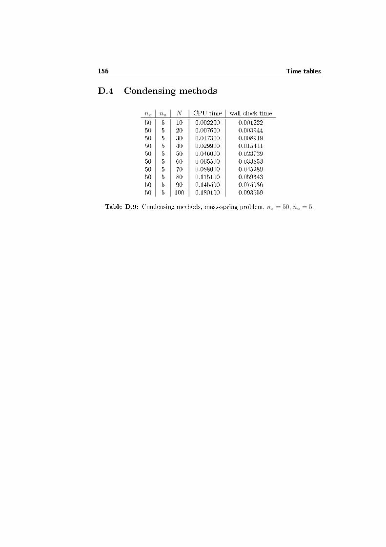
156 Time tables
D.4 Condensing methods
nx nu N CPU time wall clock time
50 5 10 0.002200 0.00122250 5 20 0.007600 0.00394450 5 30 0.017300 0.00891950 5 40 0.029900 0.01544150 5 50 0.046000 0.02372950 5 60 0.065500 0.03385350 5 70 0.088000 0.04528950 5 80 0.115100 0.05934350 5 90 0.145500 0.07503650 5 100 0.180100 0.093559
Table D.9: Condensing methods, mass-spring problem, nx = 50, nu = 5.
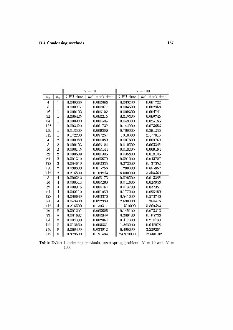
D.4 Condensing methods 157
N = 10 N = 100
nx nu CPU time wall clock time CPU time wall clock time
4 1 0.000066 0.000066 0.003200 0.0017228 1 0.000077 0.000077 0.004600 0.00235816 1 0.000102 0.000102 0.009300 0.00474132 1 0.000425 0.000215 0.019300 0.00974564 1 0.000980 0.000505 0.049000 0.025186128 1 0.003420 0.001732 0.144000 0.073656256 1 0.018500 0.009309 0.760000 0.391285512 1 0.172200 0.087287 4.310000 2.1778154 2 0.000089 0.000089 0.007300 0.0037608 2 0.000103 0.000104 0.010500 0.00534816 2 0.000145 0.000144 0.018200 0.00919432 2 0.000609 0.000306 0.035800 0.01810664 2 0.001310 0.000670 0.091000 0.045707128 2 0.004610 0.002335 0.272000 0.137352256 2 0.030300 0.015256 1.280000 0.655852512 2 0.216800 0.109843 6.600000 3.3555608 4 0.000342 0.000173 0.026500 0.01338816 4 0.000518 0.000260 0.041600 0.02098332 4 0.000915 0.000464 0.073700 0.03738164 4 0.002110 0.001080 0.177000 0.090450128 4 0.006680 0.003370 0.541000 0.273740256 4 0.043400 0.022339 2.690000 1.358476512 4 0.276500 0.139311 11.570000 5.86958316 8 0.001201 0.000605 0.145100 0.07331332 8 0.001687 0.000848 0.209100 0.10573364 8 0.004090 0.002064 0.417000 0.210739128 8 0.012560 0.006331 1.282000 0.648978256 8 0.066400 0.033912 6.400000 3.229201512 8 0.379600 0.191434 24.970000 12.680102
Table D.10: Condensing methods, mass-spring problem, N = 10 and N =100.
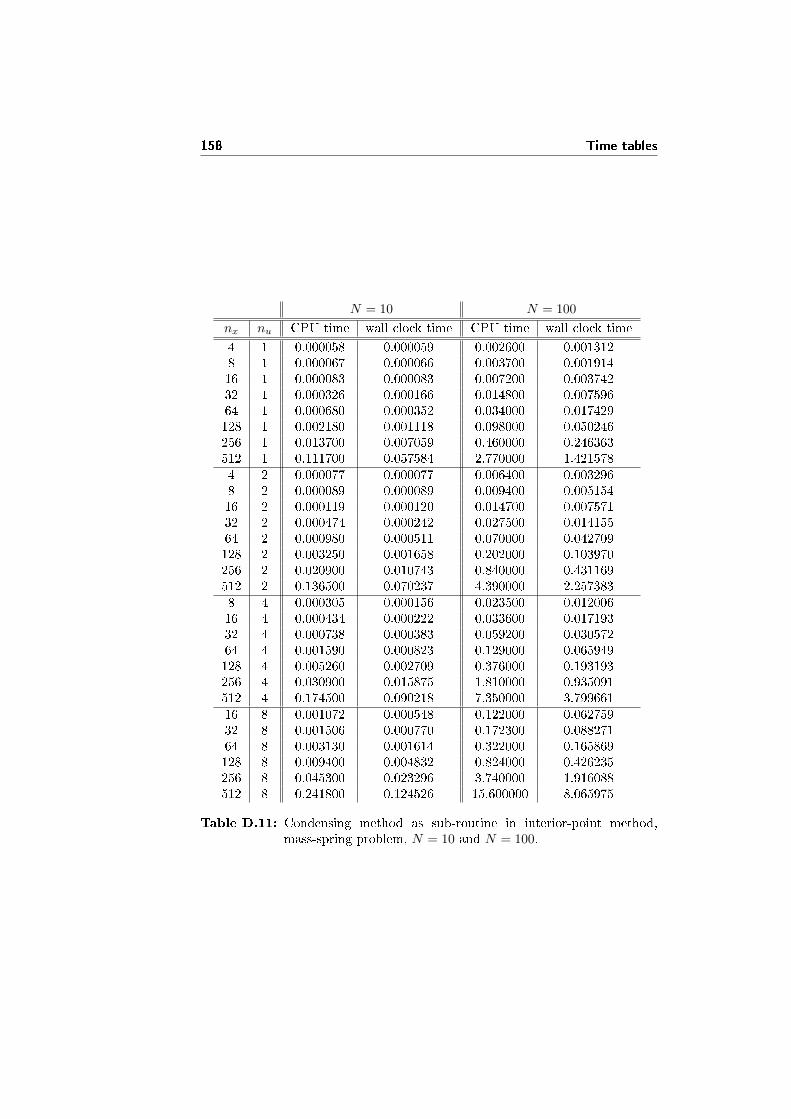
158 Time tables
N = 10 N = 100
nx nu CPU time wall clock time CPU time wall clock time
4 1 0.000058 0.000059 0.002600 0.0013128 1 0.000067 0.000066 0.003700 0.00191416 1 0.000083 0.000083 0.007200 0.00374232 1 0.000326 0.000166 0.014800 0.00759664 1 0.000680 0.000352 0.034000 0.017429128 1 0.002180 0.001118 0.098000 0.050246256 1 0.013700 0.007059 0.460000 0.246363512 1 0.111700 0.057584 2.770000 1.4215784 2 0.000077 0.000077 0.006400 0.0032968 2 0.000089 0.000089 0.009400 0.00515416 2 0.000119 0.000120 0.014700 0.00757132 2 0.000474 0.000242 0.027500 0.01415564 2 0.000980 0.000511 0.070000 0.042709128 2 0.003250 0.001658 0.202000 0.103970256 2 0.020900 0.010743 0.840000 0.431169512 2 0.136500 0.070237 4.390000 2.2573838 4 0.000305 0.000156 0.023500 0.01200616 4 0.000434 0.000222 0.033600 0.01719332 4 0.000738 0.000383 0.059200 0.03057264 4 0.001590 0.000823 0.129000 0.065949128 4 0.005260 0.002709 0.376000 0.193193256 4 0.030900 0.015875 1.810000 0.935091512 4 0.174500 0.090218 7.350000 3.79966116 8 0.001072 0.000548 0.122000 0.06275932 8 0.001506 0.000770 0.172300 0.08827164 8 0.003130 0.001614 0.322000 0.165869128 8 0.009400 0.004832 0.824000 0.426235256 8 0.045300 0.023296 3.740000 1.916088512 8 0.241800 0.124526 15.600000 8.065975
Table D.11: Condensing method as sub-routine in interior-point method,mass-spring problem, N = 10 and N = 100.
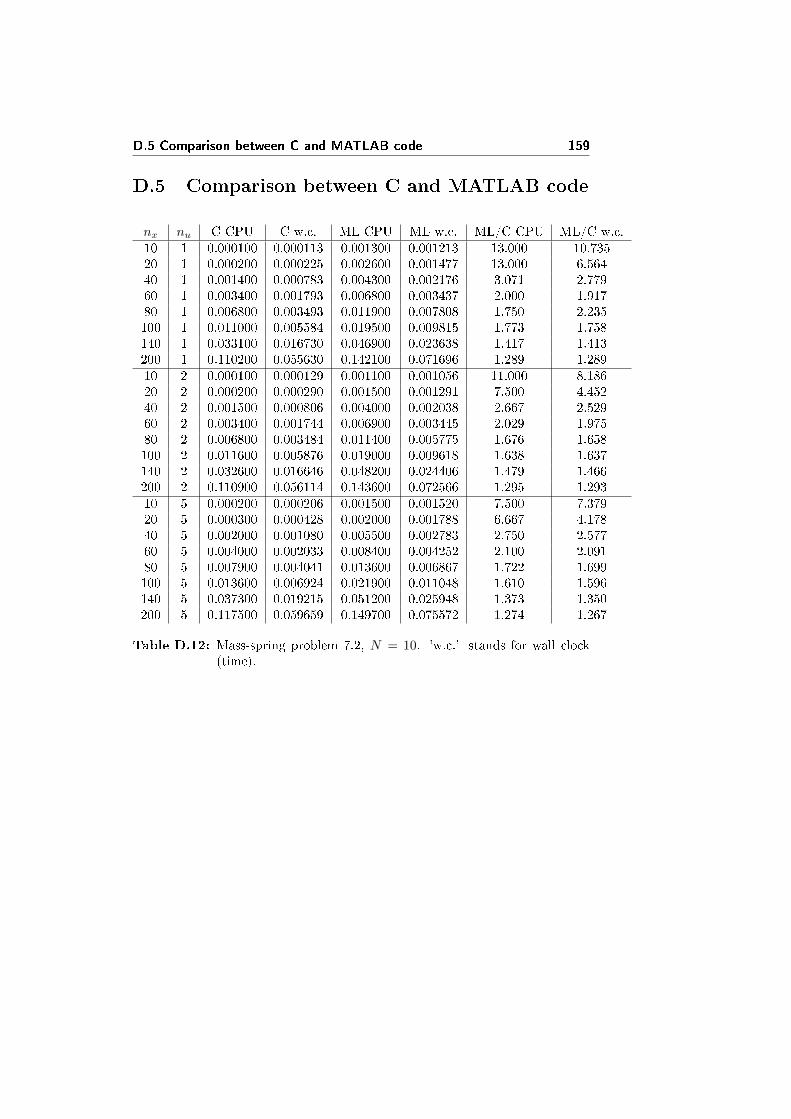
D.5 Comparison between C and MATLAB code 159
D.5 Comparison between C and MATLAB code
nx nu C CPU C w.c. ML CPU ML w.c. ML/C CPU ML/C w.c.10 1 0.000100 0.000113 0.001300 0.001213 13.000 10.73520 1 0.000200 0.000225 0.002600 0.001477 13.000 6.56440 1 0.001400 0.000783 0.004300 0.002176 3.071 2.77960 1 0.003400 0.001793 0.006800 0.003437 2.000 1.91780 1 0.006800 0.003493 0.011900 0.007808 1.750 2.235100 1 0.011000 0.005584 0.019500 0.009815 1.773 1.758140 1 0.033100 0.016730 0.046900 0.023638 1.417 1.413200 1 0.110200 0.055630 0.142100 0.071696 1.289 1.28910 2 0.000100 0.000129 0.001100 0.001056 11.000 8.18620 2 0.000200 0.000290 0.001500 0.001291 7.500 4.45240 2 0.001500 0.000806 0.004000 0.002038 2.667 2.52960 2 0.003400 0.001744 0.006900 0.003445 2.029 1.97580 2 0.006800 0.003484 0.011400 0.005775 1.676 1.658100 2 0.011600 0.005876 0.019000 0.009618 1.638 1.637140 2 0.032600 0.016646 0.048200 0.024406 1.479 1.466200 2 0.110900 0.056114 0.143600 0.072566 1.295 1.29310 5 0.000200 0.000206 0.001500 0.001520 7.500 7.37920 5 0.000300 0.000428 0.002000 0.001788 6.667 4.17840 5 0.002000 0.001080 0.005500 0.002783 2.750 2.57760 5 0.004000 0.002033 0.008400 0.004252 2.100 2.09180 5 0.007900 0.004041 0.013600 0.006867 1.722 1.699100 5 0.013600 0.006924 0.021900 0.011048 1.610 1.596140 5 0.037300 0.019215 0.051200 0.025948 1.373 1.350200 5 0.117500 0.059659 0.149700 0.075572 1.274 1.267
Table D.12: Mass-spring problem 7.2, N = 10. 'w.c.' stands for wall clock(time).
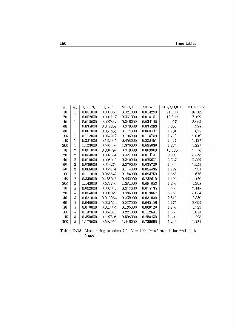
160 Time tables
nx nu C CPU C w.c. ML CPU ML w.c. ML/C CPU ML/C w.c.10 1 0.001000 0.000863 0.021000 0.014293 21.000 16.56220 1 0.002000 0.002147 0.031000 0.016101 15.500 7.49940 1 0.015000 0.007882 0.046000 0.024146 3.067 3.06360 1 0.035000 0.018307 0.070000 0.035293 2.000 1.92880 1 0.067000 0.034888 0.114000 0.058447 1.701 1.675100 1 0.112000 0.057212 0.196000 0.116709 1.750 2.040140 1 0.321000 0.162945 0.458000 0.232451 1.427 1.427200 1 1.123000 0.566469 1.376000 0.695039 1.225 1.22710 2 0.001000 0.001292 0.010000 0.009969 10.000 7.71620 2 0.003000 0.002661 0.027000 0.014737 9.000 5.53840 2 0.015000 0.008049 0.040000 0.020681 2.667 2.56960 2 0.036000 0.018279 0.070000 0.035729 1.944 1.95580 2 0.066000 0.033761 0.114000 0.058436 1.727 1.731100 2 0.111000 0.056542 0.184000 0.094759 1.658 1.676140 2 0.330000 0.168015 0.462000 0.238610 1.400 1.420200 2 1.142000 0.577790 1.381000 0.697683 1.209 1.20810 5 0.002000 0.002032 0.017000 0.015135 8.500 7.44820 5 0.004000 0.003929 0.035000 0.019857 8.750 5.05440 5 0.021000 0.010964 0.059000 0.031030 2.810 2.83060 5 0.040000 0.021524 0.087000 0.045186 2.175 2.09980 5 0.079000 0.040335 0.135000 0.069729 1.709 1.729100 5 0.137000 0.069816 0.224000 0.112631 1.635 1.613140 5 0.390000 0.197508 0.508000 0.256430 1.303 1.298200 5 1.170000 0.592969 1.446000 0.729695 1.236 1.231
Table D.13: Mass-spring problem 7.2, N = 100. 'w.c.' stands for wall clock(time).
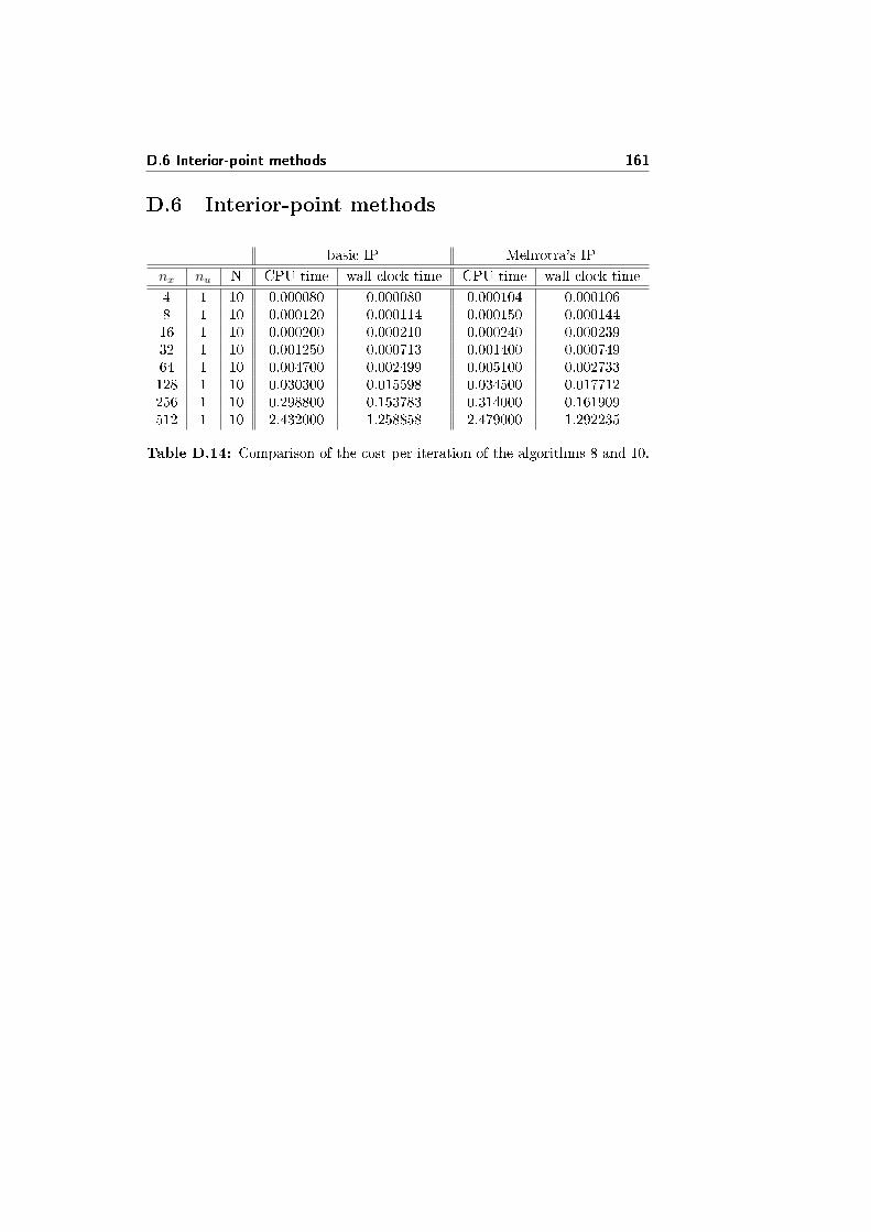
D.6 Interior-point methods 161
D.6 Interior-point methods
basic IP Mehrotra's IP
nx nu N CPU time wall clock time CPU time wall clock time
4 1 10 0.000080 0.000080 0.000104 0.0001068 1 10 0.000120 0.000114 0.000150 0.00014416 1 10 0.000200 0.000210 0.000240 0.00023932 1 10 0.001250 0.000713 0.001400 0.00074964 1 10 0.004700 0.002499 0.005100 0.002733128 1 10 0.030300 0.015598 0.034500 0.017712256 1 10 0.298800 0.153783 0.314000 0.161909512 1 10 2.432000 1.258858 2.479000 1.292235
Table D.14: Comparison of the cost per iteration of the algorithms 8 and 10.

162 Time tables
Bibliography
[Duf04] I.S. Du�. Ma57 - a new code for the solution of sparse symmetricde�nite and inde�nite systems. ACM Transactions on Mathematical
Software, 30:118�144, 2004.
[FM03] E. Fornasini and G. Marchesini. Appunti di teoria dei sistemi. Li-breria Progetto, 2003.
[Gou] B. Gough. An Introduction to GCC.
[GVDG] K. Goto and R.A. Van De Geijn. Anatomy of high-performancematrix multiplication. ACM Transactions on Mathematical Software.
[JGND12] J.B. Jørgensen, N.F. Gade-Nielsen, and B. Damman. Numericalmethods for solution of the extended linear quadratic control prob-lem. (unpublished), 2012.
[Jør05] J.B. Jørgensen. Moving Horizon Estimation and Control. PhD the-sis, Department of Chemical Engineering, Technical University ofDenmark, Kgs Lyngby, Denmark, 2005.
[KR88] B.W. Kernighan and D.M. Ritchie. The C programming Language.Prentice-Hall, 1988.
[NW06] J. Nocedal and S.J. Wright. Numerical Optimization. Springer, KgsLyngby, Denmark, 2nd edition, 2006.
[Pag07] C.G. Page. Professional Programmer's Guide to Fortran77, 2007.
[RWR98] C.V. Rao, S.J. Wright, and J.B. Rawlings. Application of interior-point methods to model predictive control. Journal of OptimizationTheory and Applications, 99(3):723�757, 1998.
[SG11] O. Schenk and K. Gärtner. PARDISO, User Guide Version 4.1.2,2011.
[Sta] R.M. Stallman. Using the GNU Compiler Collection.
[WB10] Y. Wang and S. Boyd. Fast model predictive control using onlineoptimization. IEEE Transactions on Control Systems Technology,18(2):267�278, 2010.

164 BIBLIOGRAPHY
[Wha] R. C. Whaley. ATLAS Installation Guide.