Embed Size (px)
Citation preview

UN IVERS FNIS
FACULTY OF ELECTRONIC ENGINEERING
Nil.

ORGANIZING COMMITTEE
Chairman: G.V. Milovanovic (Nis)
Secretary: M.A. Kovacevic (NiS) Members: P.M. Vasic (Beograd)
B.M. Damnjanovic (Kragujevac) R.z. Djordjevic (Nis)
P.B. Madic (Beograd) I.z. Milovanovic (Nis) M.s. Petkovic (Nis) Lj.R. Stankovic (Nis)
D.Oj. To~ic (Beograd) D. Herceg (Novi Sad)
This publication was in part supported by the Regional Association for Science- NiS and University of Nis.
Published by: Faculty of Electronic Engineering, Beogradska 14, P.O. Box 73, 18000 Nis, Yugoslavia
Printed by: Prosveta, Nis
Number of copies: 300
PREFACE
The conference "Nwnerical Methods and Approximation Theory" was held
at the Faculty of Electronic Engineering, University of Nis, September
26-28, 1984, It was attended by 46 mathematicians fPom several universities.
These proceedings contain most of the papers presentedPduring the con
ference in the form in which they were submitted by the authors. Typing,
grammatical and other errors were not, except in some isolated cases, edited
out of the received material.
The topic treated cover different problems on numerical analysis and
approximation theory.
September 1984 G.V. Milovanovid

I
I

C 0 N T E N T S
:. Bohte, M. Petkovsek Gaussian elimination for diagonally dominant matrices
M.M. Laban On some numerical properties of infinite-dimensional simplex
Lj. Cvetkovid, D. Heraeg Some sufficient conditions for convergence of AOR-method
M.S. Petkovid, L. V. Stefanovid Some modified square root iterations for the simultaneous determinati9n of multiple complex zeros of a polynomial
o.v. Slavic The generalization of ten rational approximations of iteration functions
D. v. Slavic One-point iteration functions of arbitrary convergence order
.'.J. rJojbasid On the choice of the initial approximation in solving of the operator equations by the Newton-Kantorovic method
T. Slivnik, G. Tomsic Numerical solution of the Fredholm integral equation of the first kind with logarithmic singularity in the kernel
W. Gautsahi, G.V. Milovanovid On a class of complex polynomials having all zeros in a half disc
Lj.D. Petlwvid On the optimal circular centered form
D. Dj. Tosid, D. V. TaBid Two methods for the curve drawing in the plane
B. Cigrovski, M. Lapaine, S. Petrovic . Operating with a sparse normal equations matrix
S.D. Miloradovid Approximation of 2rr - periodic functions by functions of shorter period
V.N. savid On the strong summability (C,~} of transformations of simple and multiple trigonometric Fourier series
7
13
19
27
31
37
43
49
55
61
67
73
79

,,,,J.Vasid, I.Z. Milovanovid, J.E. Pecarid An estimation for remainder of analytical function in Taylor's series
B.M. Damnjanovid On a method of numerical differentation
G. V.Milovanovid, J.E. Pecarid On an application of Hermite's interpolation polynomial and some related results
D. V. Slavic, M.J. Stanojevid Classification of formulas for n-dimensional polinomial interpolation
B. Vrdoljak On approximations of solutions of second order linear differential equations
K. Surla, E. Nikolic, Z. Lozanov On hypothesis testing in spline regression
I.E. Lackovid, Lj.M. Kocid Approximation in discrete convexity cones
Lj.M. Koeid Approximation of convex functions by first degree splines
K. Surla On the spline solutions of boundary value problems of the second order
R. Vulanovid Mesh construction fot numerical solution of a type of singular perturbation problems
D. Herceg, Lj. Cvetkovid An iterative solution of some discrete analogues of a mildly nonlinear boundary value problem
D.D. TaBid One way of discretization of Chaplygin's method
B.S. Jovanovic, Lav D. Ivanovia On a convergence of the difference schemes for the equation of vibrating string
L.D. Ivanovia, B.S. Jovanovic Approximation and regularization of control problem governed by parabolic equation
D.P. Radunovid Solutions of the grid Laplace equation defined in corners
83
87
93
99
107
113
119
125
131
137
143
149
155
161
167

1.S. Canak :onnection between one problem in elasticity theory and the method ,f approximate solving of Carlemann·s boundary value problem 173
• E. Pecaricf, M.M. Radojkovicf Solution of potential problems with internal sources by boundary element method 181
D. T. Mihailovicf A possibility for calculating Pl'essure gradient force in sigma coordinate system 187
D.M. Velickovicf A new interpretation for Green·s functions of circular conducting cylinder and its applications 193
D.M. Velickovicf Evaluation of several singular integrals using electrostatic fields lows 197

I
I
I
I
I
I
I
I
I
I
I
I
Numerical Methods and
Approximation Theory
Nis, September 26-28, 1984
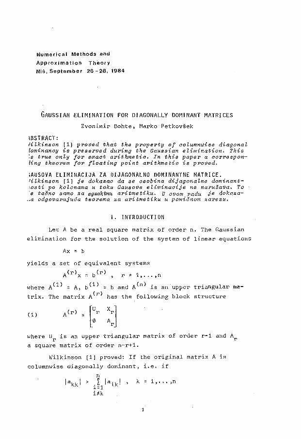
GAUSSIAN ELIMINATION FOR DIAGONALLY Dot~INANT MATRICES
Zvonimir Bohte, Marko Petkovsek
\BSTRACT: lilkinson [1] p~oved that the p~ope~ty of aolumnwise diagonal lominanay is p~ese~ved during the Gaussian elimination. This :s t~ue only fo~ exaat arithmetic. In this pape~ a aor~esponUng theorem for floating point arithmetic is p~oved.
iAUSOVA ELIMINACIJA ZA DIJAGONALNO DOMINANTNE MATRICE. lilkinson [1] je dokazao da se osobina dijagonalne dominanttosti po kolonama u toku Gausove eliminaaije ne narusava. To 'e taano samo za egzak.tnu aritmetiku. U ovom radu je dokaza-
·•a odgova~ajuda teorema za aritmetiku u pomianom zarezu.
1. INTRODUCTION
Let A be a real square matrix of order n. The Gaussian
elimination for the solution of the system of linear equations
Ax :: b
yields a set of
A(r)x
where A(1) = A,
trix. The matrix
equivalent systems
:: b(r) '
r = 1, ... ,n
b ( 1) = b and A(n) is an A(r) has the following
upper triangular ma.
block structure
where Ur is an upper triangular matrix of order r-1 and Ar
a square matrix of order n-r+1.
Wilkinson [1] proved: If the original matrix A is
columnwise diagonally dominant, i.e. if
n
, L Jaikl ' l=1
k = 1,, .• ,n
i.ik
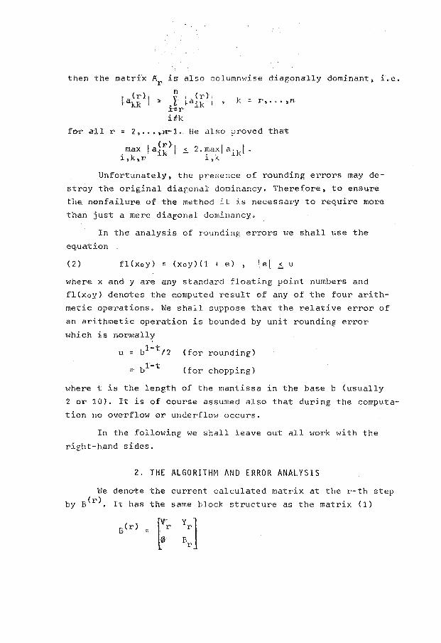
then the matri~ A is also columnwise diagonally dominant, ~.e. r
n f , (r},
.t: ~aik I J:~r-
i#k
k = r,~·· ,n
for all r = 2,~ .• ,.n-1~ He also proved that
max ~a~~}r ~ 2.max\a.kt. i,k.r I i,k 1
Unfortunately, the presence of rounding errors may de
stroy the original diagonal dominancy. Therefore, to ensure
the. nonfailure of the method it is· necessary to require more
than just a mere diagonal dorninancy.
In the analysis of rounding errors we shall use the
equation
( 2) fl(xoy) = 'xoy)(1 + e) ,
where x and y are any standard floating point numbers and
fl(xoy)- denotes the co.mputed result of any of the four arith
metic operations. vie- shall suppose that the relative error of
an arithmetic operation is bounded by unit rounding error
which is normally
u = bl-t/2 (for rounding}
(for chopping)
where t is the length of the mantissa in the base b (usually
2 or 10). It is of course assumed also that during the computa
tion no ove·rflow or underflow occurs.
In the following we shall leave out all work with the
right-hand sides.
2. THE ALGORITHM AND ERROR ANALYSIS
He denote the current calculated matrix at the r-th step
by B(r). It has the same block structure as the matrix (1)

· en t is assumed that the matrix A = B is the matrix stored-
n the computer.
'I'he algorrthm for the calculation ~f the uppeP trian
gular matrix B(n) is as f0llows:
r :: 1, .••. ,n-1:
i = r-1-1 • •.• ,n:
(3) m. ::: n(b~l"Jfbf'r·)c) 1r 1r rr
k = r+1, ••• ,n:
( 4} tf~+ 1 } = fl(bl~' -
Let us denote
i ,_k = r, .•. , n
and
(o) h = maxhr, r = 1, •.. ,n
8sing (Z} in (3) and (4) we hav-e
and
i ,k :: r+1- ,_ .•. ,n
and
( 9) t X ir ~ ' tY i~) I ' l z l~) I ~ u
Let us suppose that
(1G) [qirl ~ 1
We can write equation (7) in the form
(11) b (r+1) = b(r) _ b(r) + d{r) ik ik qir rk ik i ,k = r+1-,-· •• ,n
Hhere
d (rl __ b(r)( + (r} + (r))(! L z~rkl) + ik -qir rk xir Yik xiryik ~ •
+(b~r) - . b(r))z~r) 1k q1r rk 1k
Then we can obtain the bound for dl~) using (5), (9) and (18)
(12) fdi~)l ~ hr(2u+u 2 }(1+u) + 2uhr: (4 + 3u + u2
)uhr
Now, we can formulate the theorem.

3. THE THEOREM
Let A be a columnwise diagonally dominant matrix of
order n and furthermore, let
n (13) lakkl > .~ iaikl + cun(n-1~lakkl , k = 1, ... ,n
~=1
iotk 2 where c = 4 + 3u + u , and u is the unit rounding error.
Then the following is.true for r = 1, •.. ,n:
(i) the matrix B is columnwise diagonally dominant and r furthermore,
lb~~)l > .~ lb{~)l + cu(n-r+1)(n-r) lakkl , k = r, .•• ,n ~=r
i~k
(ii) r lb~r)l ~ j iaikl + cu(2n-r)(r-1>lakkl. k:: r, ... ,n i=r ~k ~=1
(iii) lb{~) I ~ ( 2 - cu(n-r+1) (n-r)) lakk I , i ,k = r, .•• ,n
PROOF. We shall prove the theorem by the mathematical induc
tion with respe7t to r. Let r = 1. Then, since B( 1 ) = B1 = A, proposition (i) coincides with (13). Obviously, (13) implies
that cun(n-1) < 1. Therefore, (ii) and (iii) hold trivially
for r = 1.
Let propositions (i) - (iii) hold for some r, 1 ~ r <
~ n-1, and let r+1 ~ k ~ n. From (11) and (8) we obtain
( 14) n ~ lb~r+1) I
i=r+1 ~k i~k
+ I lb~r)l i=r+1 ~k
+ I ld~r)l i=r+1 ~k
Hk i#k
From (i) and (8) it follows that the inequality (10) holds.
Therefore, we can use the bound (12) in (14). From (i) it
follows

r'Om (14) we have
n ( ) + ~ lb.kr I + cuh (n-r·~1) :::
i=r+l ~ r Hk
= i~rlbl~)l - lqkrl lb~~)l + cuhr(n-r-1)
iolkl
Finally, from (i), (iii), (11) and (12) it follows
which
~ lb<.kr+1)1 < lbk(kr)l - cu(n-~+l)(n-~>la f -L • • kl< i=r+1 ~ i~l<
- lql<rllb~~)l + 2cu(n-r-1)lakkl ~ < lb(r+1)
kk - d~~)l - cu((n-r)(n-r-1) + 2)lakkl ~
~ I b~t 1 > I + 2culakl<l - cu((n-r)(n-r-1) + 2)lal<kl ~
~ I b~~+1 >I proves ( i).
To prove (ii), note that
n (15) . L lqirl < 1
~=r+1
because B is columnwise strictly diagonally dominant. Therer fore, (11), (12}, (15) and (iii) imply that
~ ¥ lb~r)l i=r+l ~k
n ~ . I I bf~> I +
~=r
+ lb~~)l. ¥ lqirl + ¥ ld~r)l ~ ~=r+1 i=r+1 ~k
2cu(n-r)lakkl
Then, using (ii) it follows
(16) n
~ L I a · k I + cu ( 2 n- r ) ( r-1 ) I al<l< I + i=l ~
::: n 1
L la·kl + cu(2n-r-1)rlal<kl i:::1 I~
and we have obtained the same inequality (ii) in which r is
replaced by r+l.
5

6
If t·le procee~ and use the inequality (13) in Al£~ we get
~he-re fore, for each ,pair i ,k ::: r<t1, •• ~ ,n
which proves UiiL
4. CilNCLIJSIONS
The assump.tions of the 'l'heorem are suf·ficient to ensure
that the .Gaussian elimination in floating point cannot break
down. All the quotients mir are bounded in modulus by 1 and th~
pivotal growth of the computed elements is bounded by 2. There·
fore, in view of Wilkinson's error analysis [1] the .Gaussian
elimination for matrices which satisfy (13) is numerically
stable.
The Theorem also enables us to determine the minimal
length of the mantissa which ensures that the breakdown of
the Gaussian elimination cannot occur. Let the matrix A be
such that
n
~ d . L l aik l -• J.:::1
k ::: 1, ••• ,-n
i~k
The following table -shows the minimal length of the mantissa
in dependance on d and n with rounding in base 10.
minimal
r-:-:-:-:-~---· ~----n-: 5
II 1·1 :
1'5 4
I 2 3
REFERENCES:
length of the mantissa .. ·~···. ··-·-·-·--~-.
n ::: 1D n = 100 ·-------;,···----------·---9-- -- ---·;
6
5
4
4
8
7
6
6
1. WILKINSON J.H.: Error anaLysis of direct methods of matrix
inversion. J. ACM 8 (1961), 281 - 330.
erical Methods and
AppToxlmation Th:eory
J\lis, September 26-28, 1984
)l-J 80!1!:': J.:UJI1ERICAL PHOPEHS:ES OF n;J;'TlnTJ~:-DD'JENSICNAL SIEPI,EX
l\1ilos M. Laban
,BSTHAG'e!
:tarting from an analytic model of infinite-dimensional simllex in Banech space, the possil1ility of it's r:;oocl approxima;ion by one of it's finite-clirnensionel subsimplexes is obse·ved .The class of simplexes, where sue>,_ a DpJ)roxirJation is IOSsible to eip,hter make or not are established_ hy a sequen.e of theorems .Here from, the members of tl"e class of limited .nfinite-d imensioDal simplexes 1vi th vertices makin:\ the urto~onal systen,could not be BPDroximated on such a way.
1 l\EKIF I'm· ~ 1h,LJI:: OSOllll: J\1: 1;_ ;o,;~'-;}-~l ·''"1. C-Oil ;~J ',IC! C\} ~1 H PLEK;\.Pola?,eci od analitick<w moclfllR heskonBcno-c1imenzionog si
mpleksa u Banahovom prost6ru,ispituje se mogu6nost njecove dobre aproksirwcije jerlnin njer::oviu k-onocno-di111enzionirn podsimpleksorn.J;izom teorema ntvr(tu,4u se klase sirmleksa kod ko~ih je tal<:VB .'lproksimacij<J ffiOf.CUCB i one kod ko~jih nije ITlO[':Uca.Tako se dobija da ani iz klase o~rani6enih heskona~no-dimenzionih simpleksa 6ija temena cin~ ortOfODAlan sistem,ne moru biti aproksimirani na pomenuti na~in.
A finite-dimensional simplex in mathenatics ond appli
cations is widely threated notion .'2he:re exists A ere at numb
er of articles on anal;ytic-f'c~ometrical p:ronerties of a n-di
mensional simplex and, consequently 1 nu:r1erical apnlice~;ions--.
'l'he notion of infini te-dirnensional sirmlex is int1"odnced by
Bastiani in f l], and is rleveloped in topoloc::ical sense by
f.,aserick in ;-4] ,:Phelps in [5] ,Lau in 13 jt:mfl. Eollein in [2]. For a difference of such a clirection 7 \JG sh:,ll de8l with the
analytic-~eometrical approsch to tl1is notion,teepinr on mind
that infinitc'o-climensional sir,nlex I•Tould be natnral r;enerali
zation of a fini te-dir:onsional case as much ns possible .At
the samG time,we shall insist on the results which are suit
able for the numerical prnctice.
7

At first 1 we shall show that it is possible to make such a construction in at least infinite-dimensional Banach
space. The or em 1: Let X be Banach space and let x
0, x1 , ••• , xn, •.•.•
be such a vectors in X that { x1-x0
, ••• ,xn-x0
, ••• } is the infinite unconditional set of linearly independent vectors. Let us denote
+ill } ~ G x converGeS n=o n n
;{i0
, ••• ,ikJ C
C{o,1,2, ..• 1) Then S T ,where A denotes the closure of set A.
Praof: 10 Let exists sequence
( 1) limy. j -+HI) J
y be an arbitrary vector from S.Then there
(yj)(j=l,2, ••• ) of vectors from S such that +ill . +ill . .
=- y ( y ·= ~ Jg X " ""' Jg =1 • Jg ~0 ) J L_ n n ' ~ n ' n n=o n=o
states.Let us denote
It is easy to verify that
(2) YjET (j=2,3, ••• )
Since =1 ,it follows
+'<D • and by ~Jg x =Y·
n=o n n J
j . lim ( 1- 2::: Jgn) jo++ill n=O
we obtain
0
~im II ~~:- jGnxJ = 0 ,1-»ill n=J+l
If we,nov1 1 let j ~+ill in (3),then accordiw~ly to (4-) and (5) we have
lim I!Y~-y.ll 0 j-HC!D J J
•herefrom and (1) it follows
lim y~ = y j-HOD J
Herefrom,with ly !3 <; 'T •
the regard to (2),we obtain y E. T •. Consequent-
2° Let exists sequence that
z
~im zj = z ( J-HC!D
be an arbitrary vector from T ~Then there (zj)(j=l,2, •• ,) of veetors from T such
kj . . kj . . . Z • = ~ Jon Jx • ~ J,.,n=l • J,., J'h ">.O"
£- ., n n ' L- ., ' ·to' •· • • ' 'l k . "' ' J n=~ n=o J
states.Let us denote ; { j x o' • ' • ' j xk ,1 C { x o' xl' • • • ~ )
J
where
j~, n
X. jx. ' n== ~
' xn$ { jxo' • • • 'jxk,} J
It is obvious that zjES (j=l,2, ••• ).Since zj=zj ows lim z ~ =Z 'hence z E !3 •. Consequently T~S' and
j-HC!D J is completed.
,it foilthe proof
'rhis theorem allows us to use the following notion of !a infinite-dimensional simplex:
9
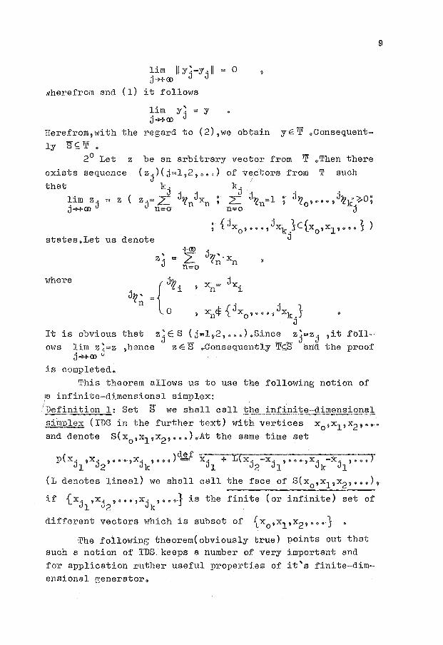
1Definition 1: Set !3 we shall call the infinite-dimensional simplex (IDS in the further text) with vertices x
0, xl' x2 , ••.•
and denote S(x0,x1 ,x2 , ••• )~At the same time set
p(x. ,x. , ••• ,x. , ••• )def x. + L(x. -x. , ••• ,x. -x. , ••• ) Jl J2 Jk Jl J2 Jl Jk Jl
(L denotes lineal) we shall call the face of S(x0,xl'x2 , ••• ),
if {x. ,x. , ••• ,x. , •••. }is the finite (or infinite) set of Jl .]2 Jk
different vectors which is subset of {x0
,x1 ,x2 , ••• }
The following theorem(obviously brue) points out that such a notion of IDS keeps a number of very important and for application ruther useful properties of it's finite-dimensional generator.

2 L · f x 1 be a fJ...nitB ·(or infin-'l'!'l.eorem : e·t ·l x . , x . , • • • ~ J. ., • • •·j JJ. J2 . k
ite) set of different vectors -which is subset of {x0 txp ........ }.
'Then.: '10 S(x. ,x. , •.••.. ,x . ., .••.•. )
J1 J2 Jk
S(x. ,x . ..,~ .•.• 1 x. , ••• ) C. p{x. ,x. , ••• ,x, , .... } ;· Jl J2 Jk Jl J2 ''k
3o p(xj~'xj2, .... ,xjk'•••j ,. p{xj21xjl'•••,x.jk'···) ~
4-o p{xJ.1
,xJ.2. , •••. .,xJ·k· , ••• ) = x. + L{x. -x. , •••. ,
· J1 .J2 Jr
2. APPH.OXIMATICN
Let S(x0,x
1, •.•• ) be an IDS.Natur8lly,the po13sibility
o:f repl8c1ng such 8 simplex with 8 finite-dimension8l .one
(FDS in the further text) is of the great importance.
At first,if supilxnll= +<D ,then S(ox:0,xl' ... ) is unlimi
ted set.and,consequently,it is not possible to replace it with an FDS which is necess8ry a limited set.If sup)lxnll< +<D,
then we have the following results~
Theore~L2,: Let { x0.,xl' ••• } be a orthoe;onal set and infllxnll =
=J..> 0 .,Then for each vector y from an arbitrary finite
dimensional subsimplex there exists a set Y(y) such that the following conditions are fulfilled:
1° Y(y),S(x0,x1 , ••• )
2° Y(y) is itself an IDS
:;0 (V:x)(;x:EY(y))(llx-yll~~)
Proof: Without loosing the generality in proof,we can obser
ve FDS S(x0
,x1 ,o-o.,xk) and such yeS(x0,x1 , •• ..,xk) that
k k Y = L'f x ( Llfn=l; lfn~o (n=O,l, •.•.• ,k))
n=o n n n=o
where 'f=-'fk = max{lfnln=O,l, ••• ,kJ. I Case l:'f;::'2' .Then Y(y)=S(xk+l'xk+2 , ••• ) •
Really, let xES( xk+l' xk+2 , • ...,.) .Since
2 1'1 ·:2 II 112. 1 112' 2 II 112>- 1/2 X-Y11 = Xi• + Y ~ tiY ~ 'fk·nXk ,y ij::O<..
; follows 3°. Case ?:If<~ .. '.rhen Y{y)=.S({l-1)xk+l+'fxk+2,(1-Yhk+l+
~xk+3 , ••• ') • r.et us ~enote
rhere
-rm +m +<D x'=( L 'f~)(l-'l')xk+l+ L 'f~·'f'xn+l={l-'fhk+ L 'f;·'f·xn+l
n=k+l n=k+l n=k+l .t follows x"ES(x
0,x1 , ••• } ,becouse
+<D (1-'1')+· L 'f"'f = I - 'f + 'f = 1
· n=k+l n
tn the base of definition 1 we can now conclude that the co
.dition 2° is fulfilled.Further on,we have
llx'-yll 2 =-llx'll 2 + Uyii 2 ~Jix'U 2 ~(1-'f') 2 11xk+l11 2>~ i..e •. 1\x''-yll>;. .Let no\'/ x be an arbitrary ve~tor £rom
Y(y).Accordin~ to definition l,there exists sequence +<D
x~=-2: 'f'(j)((l-'f)x1 1
-!''fx 1
)(j=l,2, ••• } such that x"'lim x~. J n=k+l n c+c n-1': j+HD J
Since 11xj-yll>~ (j=l,2, ••• ),there exists such a natural
number ~ 0
that \llx": -y\1 -1/x; --xlll~~
Jo Jo states,hence 3° is satisfied and the proof is completed.
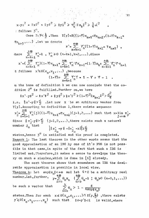
Remark 1: The last theorem in the other words means that the
good approximation of an IDS .by one of it's FDS is not poss
ible in that case,in spite of the fact that such a IDS is
limited set.Therefore,.it makes a sence to develope the theo
ry on such a simplex,which is done. in [6] already.,
The next theorem shows that somewhere on IDS the· desi-
rable approximation is possible in local view.
Theorem 4: Let sup\lxn\I<+'<D and let 't:>o be a arbitrary real +<D f'<D
number.Let,further, y=-2. g x (L_Q =1; Qn·';;l>O (n=O,l, •• .,.)) n=o n n n=o n
be such ? vector that ~ E :f;;o Qn > 1 - ..,.4-su.....;p;;;_,U,....x-n"'""ll
states.Then for each x.ES(x0,xp•••)n K(y,~) ,there exists·
y\::s(x0,x1 , ••• ,xk) such that nx--y'JI<E is valid,where
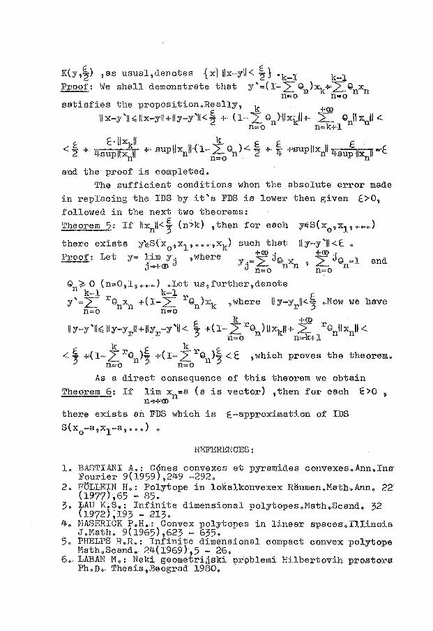
K(y,~) ,as usual,denotes {x\ llx-yll< ~} "k-1 k-1 Proof: We shall demonstrate that Y '= ( 1-L Qn )xk +'·L Qnxh
n=o n=-a satisfies the proposition.Rea11y, k -HID
llx-y'II.;;Ux'-yll+l/y-y'll<~ + (1- L Qn)·llxicll+- L Qn\lxnll < n=O n=k+l
E t . II xkll k E E. E. . < ~ +· 4suplfxn11 +- supl\xnll·(l- L Qn).::. ~ +· 'lj: +supllxJ14sup Ux II =-E
n=-0 n
and the proof is completed. The sufficient conditions when the absolute error made
in replacing the IDS by it's FDS is lower then given E.>O,
followed in the next two theorems:
Theorem 2: If 1\xnll<~ (n">k) , then for each yES(x0,xl' •.•.• )
there exists yE.S(x0,xl' ••• ,xk) such that lly-y"II<E. 0
t 1 . h +<D • +<D • Proof: Le y= ~my. ,were Y·=~Jox 2_Jg,.l and
jo++oo J J n=o n n n=o n
Q ? 0 (n=O,l, ...... ) .Let us,further,denote n k-1 k-1
y'=L_ rQnxn +(1-2: rgn)xk ,where \ly-yr\1<.~ •. Now we have n=o n=o
k +<D IIY'-y'll~ lly-yrii+IIYr-y"ll.::. ~ -r(l- .:Lron)llxkll+ L ronllxnll <
n=O n=k+1 k k
<~ +{1-zrgn)~ +(1-,Lron)~<E ,which proves the theorem. n=o n=o
As a direct consequence of this theorem we obtain
Theorem 6: If lim xn=a (a is vector) ,then for each E>O n+fo{D
there exists an FDS which is E.-approximation of IDS
S(x0-a,x1-a, ••• ) •
REFERENCES:
1. BASTIANI A.: C6nes convexes et pyramides convexes.Ann.Ins· Fourier 9(1959),249 -292.
2. HCiLLEIN H.: Polytope in loK:alkonvexex Raumen.Math.Ann •. 22 (1977),65- 85.
3. LAU K;,S .. : Infinite dimensional polytopes.Math •. Scand. 32 (197Z);I93 - 213. .
4. HASERICK P.H.: Convex polytopes in linear spaces.Iliinois J.Math. 9(1965),623- 635.
5. PHELPS R.R.: Infinite dimensional compact convex polytope f'lath.Scand. 24(1969),5- 26.
6 •. LABAN M.: Neki geometrijski prpblemi Hilbertovih prostora Ph.D •. Thesis,.Beograd 1980.
Numerical Methods and
Approximation Theory
Nis, September 26-28, 1984
SQr.'lE SUFFICIENT CONDITIONS FOR
CONVERGENCE OF AOR-METHOD
Ljiljana Cvetkovid, Dragoslav Herceg
A..BSTRl'.CT 1e consider AOR ( Accelerated Overrelaxation method for a system of n linear equations with n unknowns Ax =b,
where the matrix A has nonvanishing diagonal elements. If A is strictly diagonally dominant we improve the convergence intervals, given in [5j, for a and w. We also consider the convergence intervals for some matrices, which are not strictly diagonally dominant.
NEKI DOVODJNI USLOVI ZA KONVERGENCIJU AOR-·POSTUPKA. Posmr.·tramo AOR (Aacelerated Overrelaxation) postupak za resavanje sistema n linearnih jednacina sa n nepoznatih Ax =b, gde matrica A ima nenula dijqgonalne elemente. Ako je A strogo dijagonalno dominantna, poboljsavamo intervale konvergencije, date u l5J, za a i w. Takodje, posmatramo intervale konvergencije za neke matrice, koje nisu strogo dijagonalno dominantne.
1. INTRODUCTION
We consider a system of n linear equations with n
unknowns, written in the matrix form
Ax = b,
where the matrix A= ja .. J has nonvanishing diagonal elements, ~J-
and AOR (Accelerated overrelaxation) method for the numeri
cal solution of this linear system. This iterative method
was presented by Hadjidimos in [1!, 1978. By splitting A
into the sum D-S-T, where D =diag (a 11 ,a 22 , ... ,ann) and S
13
and T are the strictly lower and upper triang-ular parts of
A multiplied by -1, the corresponding A0R scheme has the fo
llowing form=:
(1) kH k (E-crL)x = ((1-w)E+(w-cr)L +wU)x +we, k=O,l 1 ••• 1
where L =D-rS~ lJ =D- 1T 1 c =D-1b 1 E r-s the unit matrix of or
der n.- a is the acceleration parameter 1 w 'I Q_ is the overre
laxation parameter and x 0 e en is arbitrary. The iterative.
matrix of scheme (1) is given by
M = (E-crL)- 1 ((1-wlE+.(w-o)L-I'wU)~ a, w
We get bounds fo-r the spectral radius p {M ) a-f the matrix a,w
M in form p (M ) < G and then from G < 1 we get sufficient a,w o,w -
conditions for the convergence of At!R method,
For A= !a. el e-Cn,n (= set of complex nxn matrices) we ~J
define for i=l,2,.r.,n
n p . (A} = l r a .. r I Q1. {A)
1 j;,l 1]
jh
f. =P. (U) I 1 1
2, CONVERGENCE OF THE AOR METHOD
fi=Q.(U) I - 1
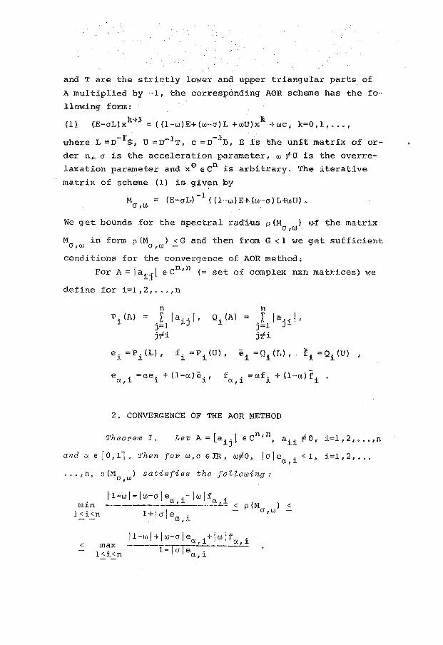
Theorem 1. r -1 n n Let A = _aij € C 1
, aii 'I 0 1 i=l I 2 I, o o In
and a € fO,ll. Then for w,a elR 1 w'fO_,. !ole . <I, i=l 1 2 1 ••• a 1 1
••• 1 n, p(M0
w) satisfies the following: ,
min l<i<n
11-w[-!w-oJe .-!w[f . -----------~-~----~~ <
I+!cr!e . al1
!1-wl+lw-crfe .+lw!f . < a,1 a 1 :t
max ---r=ra~e--. ------l<i<n a,1
Proof. We prove the upper bound for P (Ma w) • Let A
' :;,e any eigenvalue of ~'f and suppose that a,.ro
fi-wt+lw-~le +fwjf . I ' I > ---· (X ' i (X I lc I • 1 2 A 1= t I o,, In o
1-~afe ·-Ct11
After some manipulations we have
!A+w-1[ > lw+cr(/.-1) le 1+lw[f ., i=l 1 2, ... ,n 1 O:t ();~1
lbiij >aPi(B)+(l-a)Qi(B}, i=1,.2, ... ,n,
where B=[b .. ] ecn,n, B=(X+w-l)E-(w+a(l.-l))L-wU. Then 1J
l:heorem 2. 5. 2 from [2] shows that detB # 0 •. Since (E- OL) •
· ( AE-M ) = B and det (E-crL} = 1 it follows det ( l.E-M0
_} r! 0. a, w ,w
This contradicts the singularity of XE -M . a,w
The lower. bound for p(M ) one proves similarly. a, ul
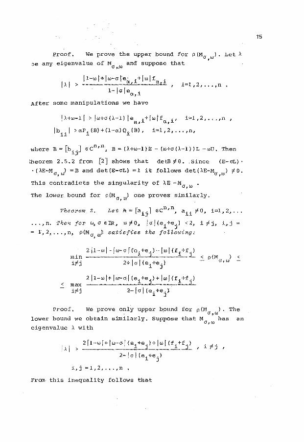
Theorem 2. Let A= [aij] ecn,n, aii '/0, i=1, 2, ...
... ,n. Then for w,a siR, wzfO, fa[(e.+e.) <2, i '/j, i,j = l. J
= I, 2, ... ,n, p(Ma w): satisfies the following: 3
min i#j
< max i;lj
2 f 1- w I - l w- a r f e . +e . J - l w r ft. +£ . > __ _;;;_J.:..... J.:._ ____ 1_J__
2+ I a I (e. +e.) 1 J
2 II-w I+ I w--ac[ ( e . +e . ) + I w f ( f . H . ) 1 L ____ !___L.
2- far fei +e:i):
Proof. We prove only upper b_ound for p (r.i ) • The a,w
lower bound we obtain similarly. Suppose that M has an a,w
eigenvalue A with
2 I 1 - w r + I w- a I c e . + e . > + I w I c £ . +£ . J I A I > _2;_1 ____ .2:_ _ _.1.._ I i 'I j I
2- I a f (e. +e . J l. J
i,j=l,2, ... ,n.
From this inequality follows that
e. +e. £.+f. ]A+w-11 >lw+o(A-1)J ..2-2_J-+jwl -~ 2-1., ir!j,i,j=1r2, ••• ,n,
1 J>-+w-1j >2 (Pi(B)+Pj(B)), ifj, i,j=1,2, ••• ,n,
where B is defined as in the proof of theorem 1. Since bii =
=>-+w-1, i=1,2, ••• ,n and
.!..2
(Pl (B) +P.(B)) >/P. (B)P.(B) • J - ~ J
we have now
I b .. I I b .. I > P . (B) P . ( B) , ii j , i , j = 1 , 2 , • • • , n • ~~ JJ ~ J
But then, theorem 2. 4.1 from [2] shows that detB f 0. This
contradicts the singularity of :\E -M0
w· , Theorem 1 contains as a special case (a=l) theorem 1
of [3], where the matrix A must be strictly diagonally domi
nant. In our case it is sufficient that A has nonvanishing
qiagonal elements.
Under assumptions of theorau 1 of [3] our theorem 2
holds, but the converse is not true.
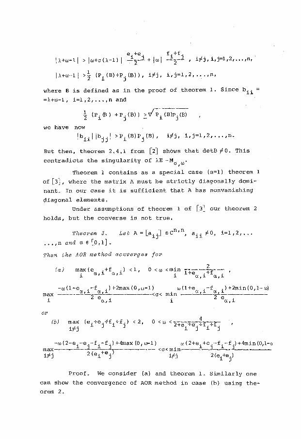
Theorem 3. Let A= [aij] eCn,n, aii fO, i=l ,2, ••.
• . • , n and a e [o, 1] .
Then the AOR method converges for
(a) max ( e . + f . ) < 1 , i a,~ a,~
2 0 < w <min
l 1 +e . +f . ... a,~ a,~
-w(1-e .-f .)+2max(O,w-1) w(1+e .-f .)+2min(O,l-w) max a'~ a'~ < < min --~~~.:!:..__ ______ _
~ 2e 4 ° 4 2e. ... a,... ... a,~
or
(b) max (e.+e.-H.+f.) <2, . ../.. ~ J ~ J ~rJ
O<w< . 4 2+e. +e·. +f. +f .
~ J ~ J
-.w (2-e. -e.-f.-f.) +4max (0 1 w-1) w ( 2+e. +e.-f.-f.) +4min (0,1-u max ~ J ~ J <o< min- ~c __ ],___.::.~_-.~.J _____ _ ·..t-· 2(e.+e.) ·..t-· 2( + ) J..r] 1. J lrJ e. e.
- 1. J
Proof. We consider (a) and theorem 1. Similarly one
can show the convergence of AOR method in case {b) using the
orem 2.
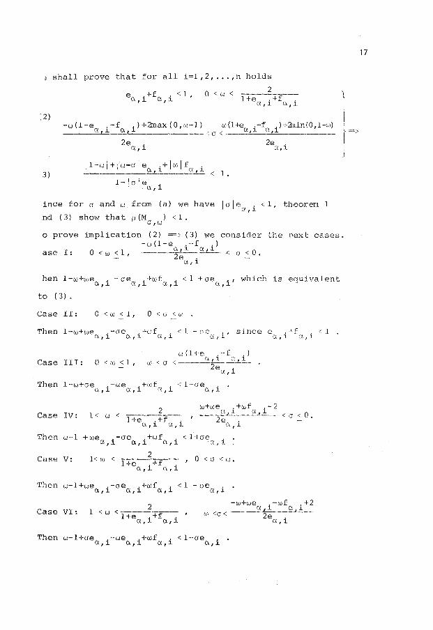
shall prove that for all i=1 1 2 1 ••• 1 n holds
e . +f . < 1 1 a 1 1. a 1 1.
-w(1-e .-f .)+2max(0 1 w-1) w(1+e .-f .)+4uin(0 1 1-w) ___ a I 1.-~-------- < o < a I J_ a 11. =>
3)
2e . 2e . a 1 1. a 11.
11-wl+lw-ale .+lw/f . ________ £..r_~--_2':..!_~ < 1.
1-lale . a11.
ince for a and w from (a) we have I a I e . < 1 1 theorem 1 a 1 1.
nd (3)
o prove
ase I:
show that p(M ) <1. a 1 w
implication ( 2) => ( 3) we consider -w(l-e .-f .)
a11. a 1 1. 0 < w < 1 I 2e . · < a < 0.
a,l
the next cases.
hen 1-w+we . - ae . +wf . < 1 + ae . I which is equivalent a 1 1. a 1 1. a 1 1. a,1.
to ( 3) •
Case II: O<w<1 1 0 <a < oJ .
Then1-w+we .-ae .+oJf .<1-oe .,sincee .+f .<1 a 1 l a,l a,l ~,l a,l a,l
Case III: O<w<l, tu ( 1 +e . - f . )
u\ < 0 < --~2:_ -...0.L~ 2e .
a 1 l
Then 1-w+oe .-we .+wf . <1-oe . a 1 l 0. 1 l a 1 l 0. 1 l
Case IV:
Then w-1 +we .-ae ,+wf . < 1+oe .. et 1 1. a 1 1. 0. 1 l et 1 l .
Case V: 2
1 < uJ < 1 +e . + f . 1 0 < o < 10 • a 1 1. a 1 l
Then w-l+we .-ae .+ulf . <1 -ae . a 1 l a 1 l a 1 1. a 1 l
Case VI: 2 1 < w < 1 +e . +f
a 1 1. o. 1 i
-w+we .-wf .+2 111 <o < __ _£_l_l __ CJ. 'l __
2e . a 1 1.
Then w-1+ae .-we .+wf . <1-ae . a 1 l 0. 1 l a,1. a 1 1.
17
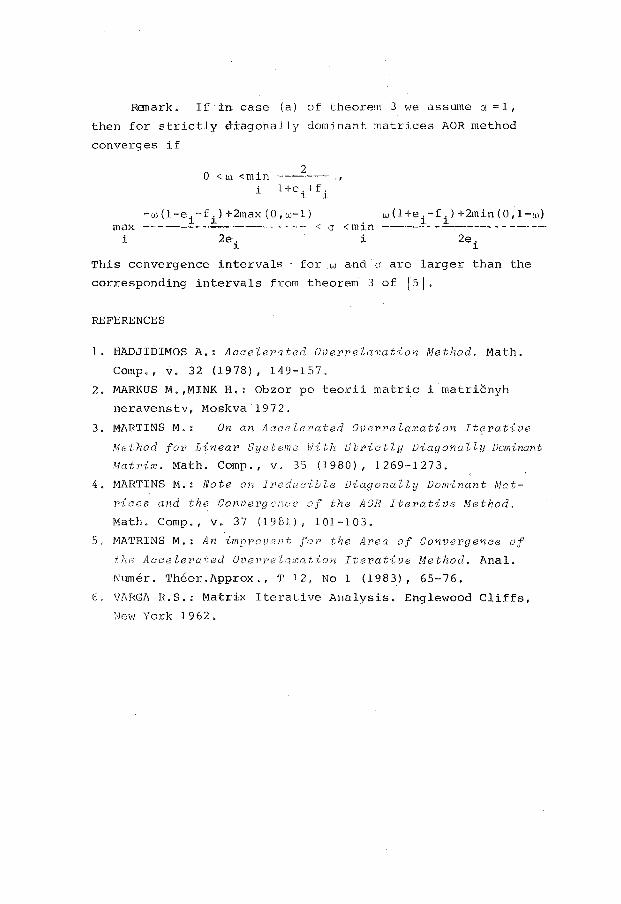
Renark. If in case (a) of theorem 3 we assume a= I,
then for strictly diagonally dominant matrices AOR method
converges if
max i
0 < w_ <min i
2
H-e.+f. l l
-uJ (1-e. -f.) +2max (0, w-1) l ~ <
2ei a <min
i
w O+e. -f.) +2m in (0.,1-w) l l
This convergence intervals · for .w and a are larger than the
corresponding intervals from theorem 3 of J5J.
REFERENCES
1. HADJIDIMOS A.: Accelerated Overl"eZa:cation Method. Math.
Comp., v. 32 (1978), 149-157.
2. MARI{US M. ,MINK H.: Obzor po teorii matric i matricnyh
neravenstv, Moskva 1972.
3. MARTINS M.: On an Accelerated OverreZaxation Iterative
Method for' Linear Systema f-lith Strictly Diagonally Dominant
Matrix. Math. Comp., v. 35 (1980), 1269-1273.
4. MARTINS M.: Note 011 IreducibZe Diagonally Dominant Mat
r•ices and the Conver'genuc of the AOR Iterative Method.
Math. Comp., v. 37 (1981), 101-103.
5. MATRINS M.: An improvcnt for the Area of Convergence of
the Accelerated Overrelamation Iterative Method. Anal.
NtmH~r. Theor.Approx., T 12, No 1 (1983), 65-76.
6. V.l\RGA R.S.: Matrix Iterative Analysis. Englewood Cliffs,
New York 1962.
Numertea-1 Methods: and
Appro>dma-tion Theory
Nis, SeptemlHH 26-28, 1984
SoME MODIFIED SQUARE ROOT ITERATIONS FOR THE SIMULTANEOUS DETERMINATION OF MULTIPLE COMPLEX ZEROS OF A POLYNOMIAL
Miodrag s. Petkovic, Lidija V. Stefanovic ABSTRACT: 4pplying Newton's and Halley~ coPrection, some modifications of squ:zre root method~ suitahle for simultaneous finding multiple complex geros of a polynomial with the known order of multiplicity, are obtained in the paper, The convergence order of the proposed (total-step) nethods is five and six respectively, Fux>ther improvements of these methods are performed by approximating to all zeros in a serial fashion 'ASing new approximations immediately they become availahle (the so-;alled Gauss-Seidel approach). Faster convergence is attained without zdditional calaulations. The lower bounds of the R-order of convergen'Je for the serial (single-step) methods are given, The considered iterative processes aPe illustrated numericaly in the example of an algebraic equation.
NEKE MODIFIKOVANE KVADRATNO KORENSKE ITERACIJE ZA SIMULTANO ODREDJIVANJE VISESTRUKIH KOMPLEKSNIH NULA POLINOMA. Primenjujudi Newtonovu i HaZleyevu koPekoiju u radu su dobijene neke modifikaoije metoda kvadratnog korena~ pogodne za simultano nalazenje visestrukih kompleksnih .nula poZinoma poznatog reda visestrukosti. Red konvergenoije predlozenih (total-step) metoda je pet i sest respektivno. Dalja poboljsanja ovih metoda su postignuta aproksimirajudi sve nule u serijskom postupku korisdenjem novih aproksimaaija odmah kada postanu dostupne (tzv. Gauss-seidelov pristup). Brza konvergencijaje dobijena bez dodatnih izraaunavanja. Za serijske (single-step) metode date su donje graniae R-reda konvergenoije. Razmatrani iterativni procesi ilustrovani su numeriaki na primeru algebarske jednaaine.
1. IrHRO-DUCTI ON
The iterative methods for the simultaneous determina
tion of mu}tip1e zeros of a polynomial have been developed du
ring the last decade as extensions of the known methods for
simple zeros. M .R. Far-mer. and G. Loizou [4] have derived a
class of iterative methods with arbitrary order of convergen
ce. The basic imperfection of methods from this class with
high convergence order (greater than three} is a demand for
great number of numerical operations t which decrease their
effectiveness. Several modifications of the basic Maehly' s
19

method [10] , which enable very fast convergence by reasonab
ly small numerical operations, have been proposed in [12] • In
recent years a lot of attention has been given to the study of
this topics in interval arithmetics (see [6] , [7], [15] , [16] ) .
In this paper we give some modifications of square root
method (also known as Ostrowski's method [14] ) which provi
de: ( i) simultaneous determination of multiple polynomial zeros
whose the multiplicities are known; ( ii) acceleration of conver
gence with small number of additional calculations in relation to
the basic method.
2. SOME MODIFICATIONS OF SQUARE ROOT ITERATIONS
Consider a monic polynomial P of degree n ~ 3
n n-1 k m. P(z) = z +an_1 z + ••• +a1z+a
0 = L (z-r.)
j=1 J (a. E C)
1
'A7 ith real or complex zeros r 1 , ••• , rk having the order of mul
'tiplicity m1' .•• ,mk recpectively, where m 1 + • • • + mk = n. Let
z 1 , •.. , zk be distinct reasonably good approximations to these
zeros and z'i be the next approximation to ri using some itera
tive sheme.
Let m be the multiplicity of the zero r of P. By the
functions
u(z)
we define
( 1) G(z)
( 2) N(z)
(3) H{z)
P'( z) P( z) v(z)
u{z) [u(z) -v(z)]
P 11 (z) p' ( z)
( Ostrow ski's function) ,
-u{~) (Newton's correction),
[ 1 -1
2 v(z)-(1+m)u(z)J (Halley's correction).
We recall that the correction terms ( 2) and ( 3) appear in the
iterative formulas
(4)
( 5)
( Shroder' s modification of Newton's method for multipie zeros, see [17]),
(modification of Halley's method, introduced by Hansen and Patrick [8] for multiple zeros),
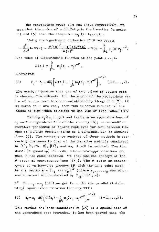
:he convergence order two and three recpectively. We
tote that the order of multiplicity in the iterative formulas
4) and ( 5) take the values m = mi (i = 1, .•. ,k).
Using the logarithmic derivative of P we obtain
d2 --z In P(z) dz
P'(z)2
- P(z)P 11 (z) =G( )= ~ ( )-2 2 z t., m. z-r.
P( z) j=1
The valv.e of Ostrowski's function at the point z =z. is 1
k <;' ( )-2 t., m. z. - rJ.
j=1 J 1
wherefrom
(6)
-1/2
). m.(z.-r.)-2 ] (i=1, ••• ,k). jjli J 1 J *
The symbol *denotes that one of two values of square root
is chosen. One criterion for the choice of the appropriate va
lue of square root has been established by Gargantini [7], If
all zeros of P are real, then this criterion reduces to the
choice of sign which coincides to the sign of (real value) PP;
r. on J
Setting r. i:! z. in ( 6) and taking some approximations of 1 1
the right-hand side of the identity ( 6), some modified
iterative processes of square root type for simultaneous fin-
ding of multiple complex zeros of a polynomial can be obtained
from ( 6) • The convergence analyses of these methods is ess
entially ·the same to that of the iterative methods considered
in [1], [2, Ch. 8], ~1], and so, it will be omitted. For the
serial (single-step) methods, _where new approximations are
used in t:he same iteration, we shall use the concept of the
R-order of convergence (see [13]). The R-order of conver
gence of an iterative process IP with. the limit point given
by the vector r; = [r1 · • • rk] T (where r 1 , •.. ,rk are poly
nomial zeros) will be denoted by OR ( (I P) , r) •
1° For r.: = z. (j f i) we get from (6) the parallel (total-J J
step) square root iteration (shortly TS):
( 7)
This method has been considered in [15] as a special case of
the generalised root iteration. It has been proved that the
21
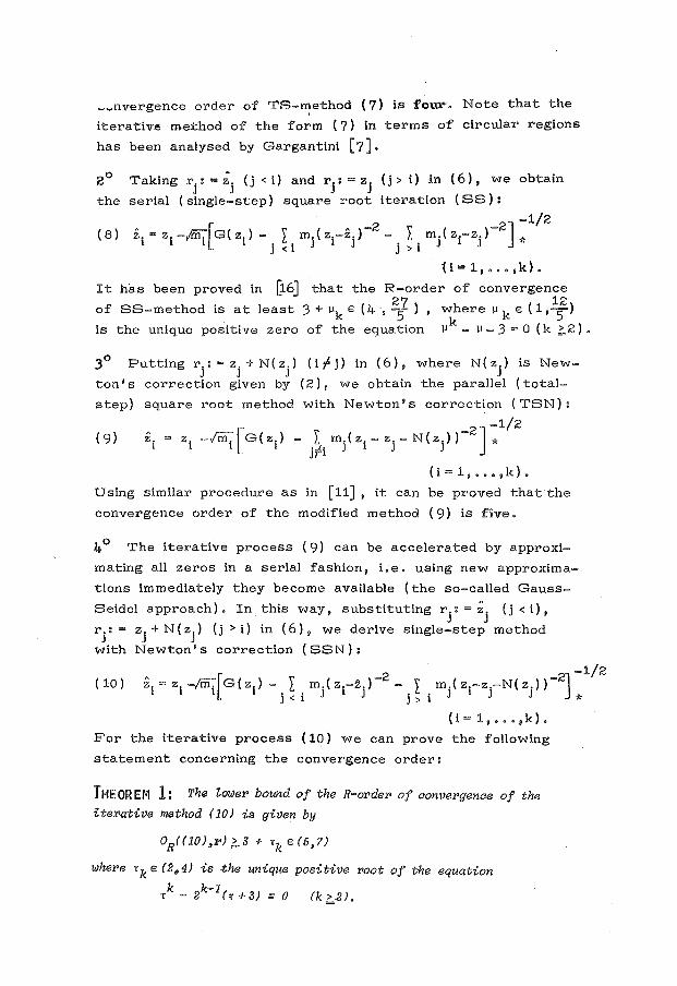
__ nvergence order of TS-method ( 7) is four. Note that the I
iterative m-ethod of the form { 7) in terms of circular regions
has been analysed by Gargantini [ 7] .
the
(8)
Taking r.: =~. (j <i) and rj: =z. (j> i) in {6), we obtain J J . J
serial (single-step) square root iteration ( SS):
-1/2 z.=z.-vfn.[G(z.)- I m.(z.-z.)-2 - I m.(z.-z.)-2 ]-~~
l l l l j<i .l l J j>i J 1 J
(i=1, ••• ,k).
It has been proved in [16] that the R-order of convergence
of SS-method is at least 3+llkE(4·,257 ), where\.lkE(1,
1;)
k is the unique positive zero of the eq1,1.a tion \.1 - Jl- 3 = 0 ( k ~,2) •
3° Putting r.:=z.+N(z.) (itj) in (6), where N(z.) is New-J J J J
ton's correction given by (2), we obtain the parallel (total-
step) square root method with Newton's correction ( TSN):
2] -1/2 (9) z 1 zi -/m."[G(z.)- I m.(z.-z.-N(z.))- *
1 1 jti J 1 J J
(i=1, ••• ,k).
Using similar procedure as in [11] , it can be proved that the
convergence order of the modified method ( 9) is five.
4 ° The iterative process ( 9) can be accelerated by approxi
mating all zeros in a serial fashion, i.e. using new approxima
tions immediately they become available (the so-called Gauss
Seidel approach). In this way, substituting r.: = ~. (j < i), J J
r.: = z. + N(z.) (j > i) in (6), we derive single-step method J J J
with Newton's correction ( SSN):
A [ -2 -2] -1/2 (10) z.=z . .,lffi, G{z.)- L m.(z.-z.) - L m.(z.-z.-N(z.)) l I 1 l j<i J l J j>i J l j J *
( i = 1' ••• .,k).
For the iterative process { 10) we can prove the following
statement concerning the convergence order:
THEOREM l; The ~(JIJ)er bound of the R-o't'der of oonvergenae of the
iterative method (10) is given by
OR((lO),J!') ~3 + Tk E (5,7)
where Tk E (241 4) is the unique positive root of the equation
/-2k-l(t+3)=0 (k~-2).
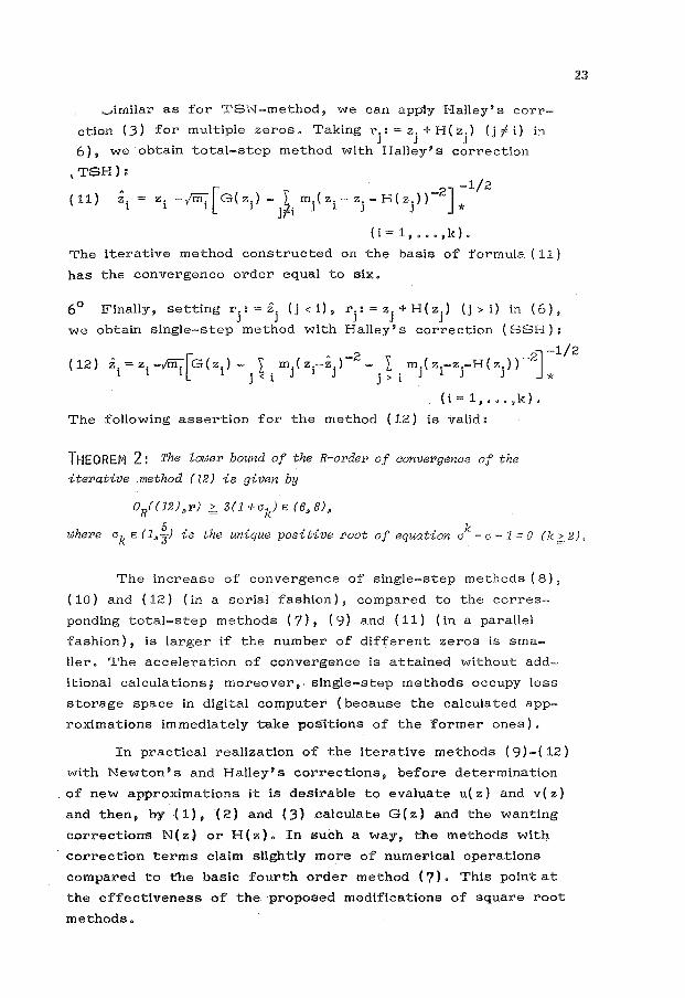
._,imilar as for TSN-method, we can app1y Halley's corr
ction (3) for multiple zeros. Taking r.: = z. + H(:z.) (j f i) in J J J
6), we obtain total-step method with Ha11ey' s correction
,TSH):
z. = z. -,liil;[G(z.)- Y m.(z.-z.-H(z.))-2]-1
/2
(11) 1 1 1 1 jFi .1 1 J J . *
(i=1, ••• ,k).
The iterative method constructed on the basis of formula ( 11)
has the convergence order equal to six.
6° Finally, setting r.:=z. (j<i), r.:=z.+H(z.) (j>i) in (6), J J J J J
we obtain single-step method with Ha11ey' s correction ( SSH):
23
J -1/2
{12) z.=z.-,r'i1;'fG(z.)- I m.(z.-z.)-2 - I m.(z.-z.-H(z.))-2 I I IL I j<i J 1 J j>i J I J J *
(i=1, ... ,k).
The fo11owing asser·tion for the method ( 12) is valid:
THEOREM 2: The lower bound of the R-order of convergence of the
iterative .method (12) is given by
OR((12),p} ~ 3(1 +ak) E (6,8),
where ak E ( 1,-i) is the unique positive root of equation l- a- 1 = 0 (7< ~- 2).
The increase of convergence of single-step methods ( 8) ,
( 10) and ( 12) (in a serial fashion) , compared to the corres
ponding total-step methods ( 7), ( 9) and ( 11) (in a para11el
fashion), is larger if the number of different zeros is sma
ller. The acceleration of convergence is attained without add
itional calculations; moreover,. single-step methods occupy less
storage space in digital computer (because the calculated app
roximations immediate!¥ take positions of the former ones).
In practical realization of the iterative methods ( 9 )-( 12)
with Newton's and Halley's corrections, before determination
. of new approximations it is desirable to evaluate u( z) and v( z)
and then, by (1), (2) and {.3) calculate G(z) and the wanting
corrections N(z) or H(z). In such a way, the methods with
correction terms claim slightly more of numerical operations
compared to tbe basic fourth order method ( 7) • This point at
the effectiveness of the ·proposed modifications of square root
methods.
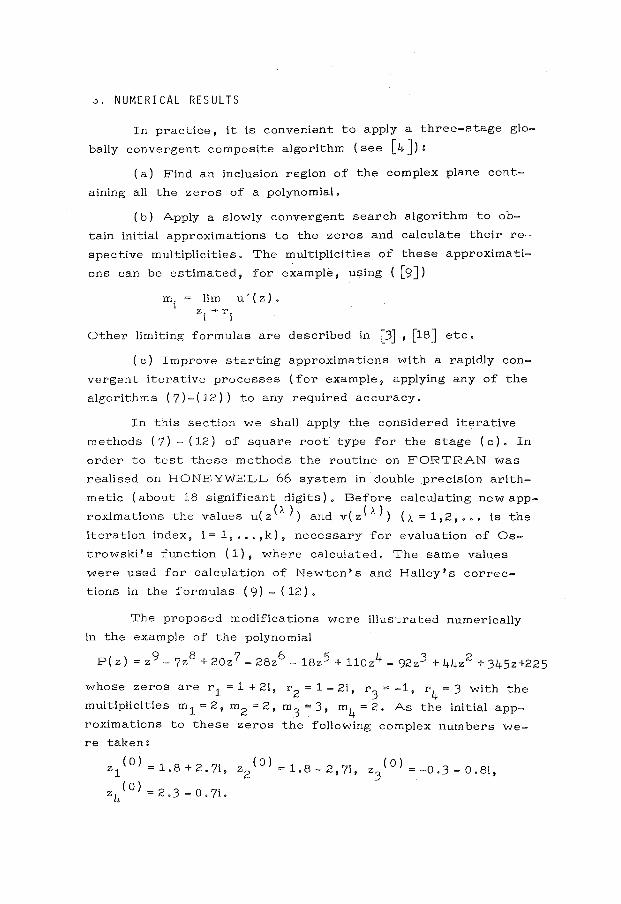
.), NUMERICAL RESULTS
In practice, it is convenient to apply a three-stage glo
bally convergent composite algorithm (see [ 4]) :
(a) Find an inclusion region of the complex plane cont
aining all the zeros of a polynomial.
(b) Apply a slowly convergent search algorithm to ob
tain initial approximations to the zeros and calculate their re
spective multiplicities. The multiplicities of these approxima ti
ons can be estimated, for e~ample, using ( [9])
m. = lim 1
u' ( z). z. -+ r.
1 1
Other limiting formulas are described in [3] , [18 J etc.
(c.) Improve starting approximations with a rapidly con
vergent iterative processes (for example, applying any of the
algorithms ( 7) -( 12)) to any required accuracy.
In this section we shall apply the considered iterative
methods (7)- (12) of square root type for the stage (c). In
order to test these methods the routine on FORTRAN was
realised on HONEYWELL 66 system in double precision arith
metic (about 18 significant digits). Before calculating new app
roximations the values u(z('-)) and v(z('-)) (t- =1,2, •.• is the
iteration index, i = 1, •.• ,k), necessary for evaluation of Os
trowski's function ( 1) , where calculated. The same values
were used for calculation of Newton's and Halley's correc
tions in the formulas ( 9) - ( 12).
The proposed modifications were illustrated numerically
in the example of the polynomial
P( z) = z 9 - 7z8
+ 20z 7 - 28z6 - 18z 5 + 11oz4 - 92z3 + 44z 2 + 345z+225
whose zeros are r 1 = 1 + 2i, r2
= 1- 2i, r3
= -1, r4
= 3 with the
multiplicities m 1 = 2, m 2 = 2, m3
= 3, m4
= 2. As the initial app
roximations to these zeros the following complex numbers we
re taken:
z 1 (0) =1.8+2.7i, z2
(0) =1.8-2,7i, z3
(0) =-0.3-0.8i,
( 0 ) - 2 3 0 7' z4 - . - . 1.
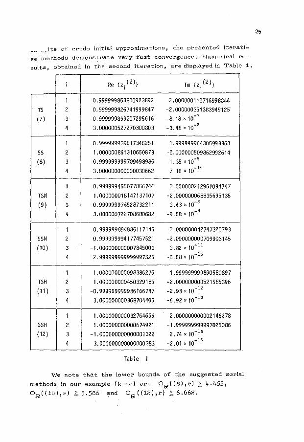
~·· - ... Jte of crude initial c•.pproxima tions, the presented it era ti
ve methods demonstrate very fast convergence. Numerical re
sults, obtained in the second iteration, are displayed in Table 1.
i Re { z ( 2)} Im{z.( 2)} i 1
1 0.999999853800923892 2.000000112716998844
TS 2 0.999999826741999847 -2.000000351383949125
(7) 3 -0.999999859207295616 ··8.18 X 10- 7
4 3.000000527270300803 -3.48 X 10⁻⁸
1 0.999999939617346251 1.999999964305993363
ss 2 1.000000861310650873 -2.000000509862992614
(8) 3 0.999999999709498985 1. 35 X 10-9
4 3.000000000000030662 7,16 X 10-llf
1 0.999999455077856744 2.000000212961094747
TSN 2 1.000000018147137107 -2.000000068835695135
(9) 3 0.999999974528732211 3,43 X 10⁻⁸
4 3.000000722708680682 -9,58 X 10 -8
1 0.999999894885117145 2,000000042747320793
SSN 2 0.999999994177457521 -2.000000000709903145
( 10) 3 -1.000000000007845003 3.82 X 10-ll
4 2.999999999999997525 -6.58 X 10- 15
1 1.000000000098386276 1.999999999890580897
TSH 2 1.000000000450329186 -2.000000000521585396 ( 11 ) 3 -0.999999999986166747 -2.93x10- 12
4 3.000000000368704406 -6.92 X 10- 10
1 1.000000000032764666 2.000000000002146278 SSH 2 1.000000000000674921 -1.999999999997025086 ( 12) 3 -1.000000000000001322 2. 74 X 10- 15
4 3.000000000000000383 -2,01 X 10 -16
Table 1
We note that the lower bounds of the suggested serial
methods in our example (k=4) are OR((8),r) ~ 4.453, OR ( ( 10 ) , r) ,;, 5. 586 and OR ( ( 12) , r) ~ 6. 662 •
25
REFERENCES
1. ALEFELD G., HE'.RZBERGER J.: On the convergence speed of some algorithms £or the simultaneous approximation of polynomial roots. SIAM J. Numer. Anal. 2(1974),237-243.
2. ALEFE'.LD G., HERZBERGER J.: E'·infi.ihrung in die Intervallrechnung. B. I. Wissenschaftsverlag, ZUrich 1974.
3. DEKKER T. J.: Newton-Laguerre iteration. Colloq. Internat. CNRS no. 165. Programmation en mathematiques numeriques 1968, 189-2{)0.
4. FARMER M.R., LOIZOU G.: An algorithm for the total or partial factorization of a polynomial. Math. Proc. Cam b. Phil. Soc. 82 (1977), 427-437.
5. GAR GANTI NI I. : Parallel Laguerre iterations: Complex case. Numer. Math. 26 (1976), 317-323.
6. GARGANTINI I.: Further applications of circular arithmetic: Schroeder-like algorithms with error bounds for finding zeros of polynomials. SIAM J. Numer. Anal. 3 ( 1978), 497-510.
7. GARGANTINI I.: Parallel square-root iterations for multiple roots. Comput, Math, with Appl. 6 ( 1980) , 279-288.
8. HANSEN E., PATRICK M,: A family of root finding methods. Numer. Math. 27 ( 1977), 257-269.
9. LAGOUANELLE J. L. : Bur une methode de calcul de 1' ordre de multiplicite des zeros d 'un polynome. C. R. A cad. Sci. Paris A 262 ( 1966), 626-627.
10. MAE'.HL Y H. J.: Zur iterativen Auflosung algebraischer Gleichungen. Z. Angew. Math, Phys. 5 ( 1954) , 260-263.
11. MILOVANOVIC G. V., PE'.TKOVIC M. B.: On the convergence order of a modified method for simultaneous finding polynomial zeros. Computing 30 (1983), 171-178.
12. MILOVANOVIC G, V,, PE.TKOVIC M.S.: Metodi visokog reda za simultano odredjivanje vi&estrukih nula polinoma. Zbornik V znanstvenog skupa PPPR, Btubicke Toplice 1983, 95-99.
13, ORTE.GA J .M., RHE.INBOLDT W.C.: Iterative solution of nonlinear equations in several variables, Academic Press, New York 1970.
14.
15.
OSTROWSKI A.M.: Solution of equations and systems of equations, Academic Press, New York 1966,
PE'.TKOVIC M.S.: Generalised root iterations for the simultaneous determination of multiple complex zeros. ZAMM 62-( 1982)' 627-630. .
, 16. PE'.TKOVIC M.S., BTE.FANOVIC L.V.: On the conver
gence order of accelerate.d root iterations. Numer. Math. (to appear) ,
17. SCHRODE-R E..: Uber unendhch viele Algorithmen zur Auflosung der Gleichungen. Math; Ann. 2 (1870), 317-365.
18. TRAUB J. F. : Iterative methods for the soilution of equations. E-nglewood Cliffs, New Jersey~ Prentice Hall 1964.
r•u,nerica I Methods and
App rox i mat ion Theory
Nis, September 26-28, 1984
ABSTRACT:
THE GENERALIZATION OF TEN RATIONAL APPROXIMATIONS OF ITERATION FUNCTIONS
Dusan Ve Slavic
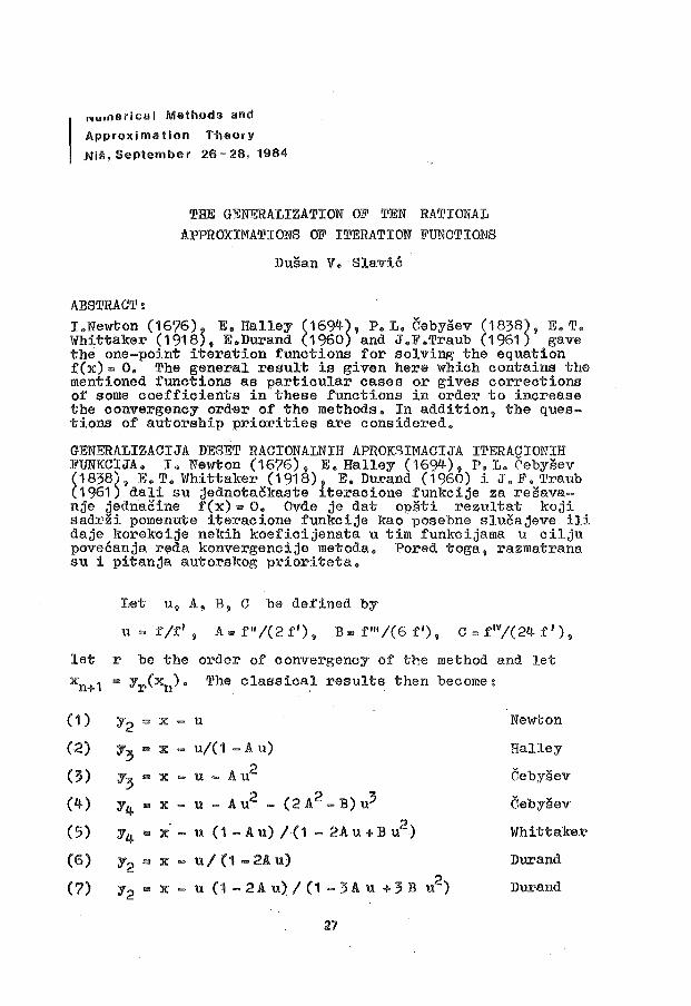
I .Newton (1676) ~ E. Halley (1694), P. L. Cebysev (1838), E. T. Whittaker (1918) 9 E.Durand (1960) and J.F.Traub (1961) gave the one-point iteration functions for solving the equation f(x)= o. The general result is given here which contains the mentioned functions as particular cases or gives corrections of some coefficients in these functions in order to increase the convergency ord~r of the methods. In addition, the questions of autorship priorities are considered.
GENERALIZACIJA DESET RACIONALNIH APROKSIMACIJA ITERACIONIH FUNKCIJA. I. Newton (1676), E. Halley (1694), P. L. Cebysev (1838), E. T. Whittaker (1918) 1 E. Durand (1960) i J. F. Traub (1961) dali su jednotackaste 1teracione funkcije za resavanje jednacine f(x)• o. Ovde je dat opsti rezultat koji sadrzi pomenute iteracione funkcije kao posebne slucajeve ili daje korekcije nekih koeficijenata u tim funkcijama u cilju povecanja reda konvergencije metoda. Pored toga, razmatrana su i pitanja autorskog prioriteta.
Let u, A, B, C be defined by
u"' f/f1, A,.f"/(2f1
), B=f111 /(6f1), C=f1v/(24f 1 ),
let r be the order of convergency of the method and let xn+i • Yr(xn)• The classical results then become:
(1) y2 .. X - u Newton
(2) 7:; "" X- u/(1-Au) Halley
(3) Y:; "'X 2 - u- Au Cebysev
(4) y4 .. X- u - A u2 - ( 2 A 2 - B) u3 Cebysev
(5) y4 "' X-U (1 -Au) /(1 - 2A u + B u2) Whittaker
{6) y2- X - u/ (1- 2A u) Durand
(7) y2 .. X - u (1-2Au)/(1-3Au+3B u2) Durand
27
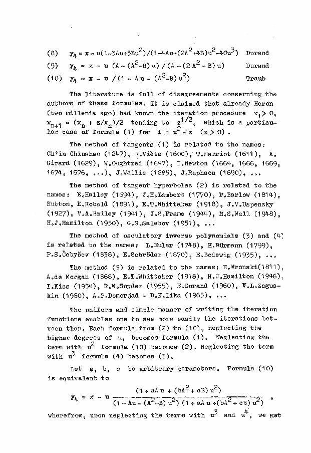
(8) y4 .. x- u(1-3Au+3Bu2)/(1-4Au+(2A2+4B)u2-4cu3) Durand
(9) y4 "" x - u (A- (A2-B) u) I (A- (2 A2 - B) u) Durand
(10) y4 .. x-u /(1- Au- (A2-B)u2) Traub
The literature is full of disagreements conserning the authors of these formulas. It is claimed that already Heron (two millenia ago) had known the iteration procedure x1) o, xn+1 = (xn + z/xn)/2 tending to z112 , which is a particular case of formula (1) for f = x2 - z (z) 0).
The method of tangents (1) is related to the names: Ch'in Chiushao (1247), F.Vi~te (1600), T.Harriot (1611), A. Girard (1629), W.Oughtred (1647), I.Newton (1664, 1666, 1669, 1674, 1676, ••• ), J.Wallis (1685), J.Raphson (1690), •••
The method of tangent hyperbolas (2) is related to the names: E.Halley (1694), J.H.Lambert (1770), P.Barlow (1814), Hutton, E.Kobald (1891), E.T.Whittal{er (1918) 9 J.V.Uspensky (1927), V.A.Bailey (1941), J.S.Frame (1944), H.S.Wall (1948) 9
H.J.Hamilton (1950) 9 G.s.Salehov (1951), •••
The method of osculatory inverse polynomials (3) and (4: is related to the names: L.Euler (1748), H.BUrmann (1799), P.S.Cebysev (1838), E.Schroder (1870), E.Bodewig (1935), •••
The method (5) is related to the names: H.Wronski(1811) 1
A.de Morgan (1868), E.T.Whittaker (1918), H.J.Hamilton (1946)~ I.Kiss (1954), R.W.Snyder (1955), E.Durand (1960), V.L.Zaguskin (1960), A.P.Domorjad- D.K.Lika (1965), •••
The uniform and simple manner of writing the iteration functions enables one to see more easily the iterations betveen then. Each formula from (2) to (10), neglecting the higher degrees of u, becomes formula (1). Neglecting the term with u2 formula (1 0) becomes (2). Neglecting the term with u3 formula (4) becomes (3).
Let ~' b, c be arbitrary parameters. Formula (10) is equivalent to
(1 + aA u + (bA2 + cB) u2 )
y4 "' x - u (1 -Au- (A2-B) u2) (1 + aA u +(bA2 + cB) u2) '
wherefrom, upon neglecting the terms with u3 and u4 , we get
29
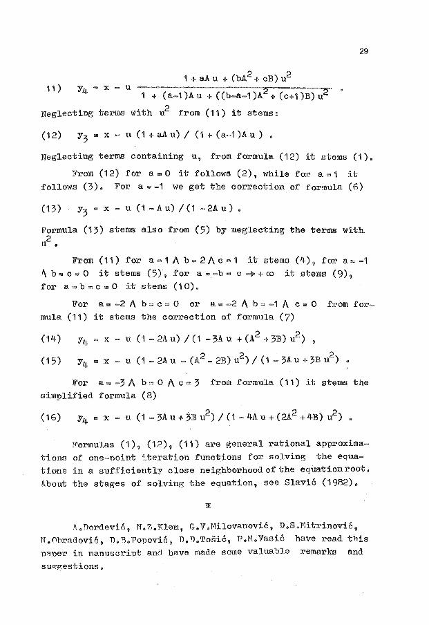
11) 1 + (a-1 )Au + ( (b-a-1 )A2 + (c+1 )B) u2
Neglecting terms with u2 from (11) it stems:
(12) y3
= x - u (1 + aA u) I (1 + (a-1)A u ) •
Neglecting terms containing u, from formula (12) it stems (1).
From (12) for a= 0 it follows (2), while for a"' 1 it
follows (3). For a= -1 we get the correction of formula (6)
( 13) y 3 "' X - u ( 1 - A u) I ( 1 - 2A u ) •
~ormula (13) stems also from (5) by neglecting the terms with
u2 •
From (11) for a=1A b=2/\c=1 it stems (4), for a=-1
f\ b = c = 0 it stems (5), for a = -b = c ...,. + ro it stems (9),
for a =b = c = 0 it stems (10).
For a= -2 1\ b = c = 0 or a= -2 A b = -1 A c = 0 from formula (11) it stems the correction of formula (7)
( 14) y 4 = x - u ( 1 - 2A u) I ( 1 - 3A u + (A 2 + 3B) u2 )
(15)
For a= -3 A b = 0 1\ c = 3 from formula (11) it stems the simplified formula (8)
Formulas (1), (12), (11) are general rational approxima
tions of one-noint ~teration functions for solving the equations in a sufficiently close neighborhood of the equation root,
About the stages of solving the equation, see Slavic (1982).
A.Dordevi6, N.Z.Klem, G.V.JI1ilovanovi6, D.S.Mitrinovi6 9
N.Obradovic, n.B."Popovi6, D.D.Tosi6, :P.H.Vasi6 pRper in manuscript and have made some valuable
sur:r;estions.
have read this remarks and
REFERENCE.S
1. CEBYPEV P.L.: Vycislenie korney uravnenija. Y..foskva 1848.
2. DURAND E.: Solutions numeriques des 'quations alg,briques, I. Paris 1960.
3. F..AJ.IilW E. : A new, exact and easy method of finding the roots of equations generally, and that without any previous reduction. Phil.Trans.Roy.Soc.London 18(1694)136-145.
4. NEivTON I.: J,etter to G.ii/.Leibniz, 13.6.1676.
5. SLAVIC D.V.: Solution of equations by function modification. Univ.Beograd. Publ.Elektrotehn.Fak. Ser.Mat.Fiz. N°735-762 (1982) 127-129.
6. TRAUB J.F.: On a class of iteration formulas and some historical notes. Comm.ACM 4(6) (1961) 276-278.
7. ':lRITTAKER B.T.: A formula for the solution of algebraic or transcendental equations. Proc.Edinburgh Math.Soc. 36(1918) 103-106.
'I Numeri-cal Methods and 1 Approximation Theory
' Nis, September 26-28, 1984
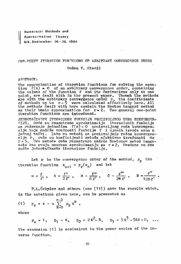
ONJ':-POINT ITERATION FUN0TIONS OF ARBITRARY CONVERGENCE ORDER
Dusan v. Slavic
AB<iTRACT: The approximation of iteration functions for solving the equation f(x) • 0 of an arbitrary convergence order, containing the values of the function f and its derivatives only at one point! are dealt with in the present paper. Though the methods are \nth the arbitrary convergence order r, the coefficients of methods up to r = 5 were calculated effectively here. All the methods dealt with here contain the Newton tangent method as their basic approximation for r= 2. Two general one-point iteration functions are introduced. JEDNOTACKA~T~ ITER~CIONE FUNKCIJE PROIZVOLJNOG REDA KONVERGENCIJE. Ovde su razmatrane aproksimacije iteracionih funkcija za resavanje jednacina f(x) = 0 proizvoljnog reda konvergencije koje sadrze vrednosti funkcije f i njenih izvoda samo u jednoj tacki. Iako su metodi sa proizvoljnim redom konvergencije r, ovde su koeficijenti metoda efektivno izracunati do r = 5. Sve metode ovde razmatrane sadrze Newtonov metod tangenata }{ao svoju osnovnu aproksimaciju za r "'2. Uvedene su dve opste jednotackaste iteracione funkcije.
Let r be the convergence order of the method, Yr the iteration function ~+1 = Yr(xn) and let
f u =f'
f" A "' 2 f' '
f'" c = --24 f 1
'
P.L.Cebysev and others (see t1tl) gave the results which, in the notations given here, can be presented as
r-2 ( 1 ) y = x - u " pk uk
r k';:o where
2 p2 = 2 A - B, 3 p3 "" 5 A - 5AB + C, •••
The exnansion (1) is equivalent to the power series of the in
verse function.
31
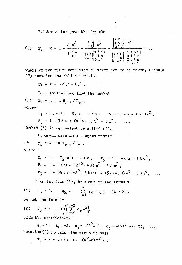
E.T.Whittaker gave the formula
lAB Cl u4 A u2 lt~l u
3 1 A B u 1 A (2) Yr "' X - u ---- ,_ GOO
1 1~ tl 11 All~ t ~I '1 A Bl
1 ABC u1AB
u 1 Ou 1 u1A Ou1A 0 u 1 0 Ou 1
where on the right hand side r terms are to oe taken. Formula
(2) contains the Halley for~ula.
y3 "" x - u I ( 1 -Au) •
E.T.Hamilton provided the method
( 3) Y r = x - u Rr-i I Rr ,
'\<!here
R1 "" R2 = 1 , R3 = 1 - A u , R4 = 1 - 2 A u + B u2 ,
R5 = 1 - 3 Au + (A2 + 2 B) u2 - C u3 ,
Method (3) is equivalent to method (2).
E.Durand gave an analogous result:
( 4) Yr = x - u Tr_1 I Tr ,
\!There
T1 = 1 '
T4 :::: 1
T5 = 1
Starting
(5)
T2 = 1 - 2A u, T3 "' 1 - 3A u +
- 4 A u + ( 2 A 2 + 4 B) u2 - 4 C u3 ,
- 5Au+ (6A2 + 5B) u2 - (5AB+ 5C)u3 +
from (1), by means of the formula
k qk "' - L P· qk_1· (k '> 0) ,
i=1 J.
we get the formula
(6)
with the coefficients:
3 B u2 ,
5D u4 ,
qo = 1' q1 = -A, q 2 "' -(A2-B), q'3 = -(2A3 -3AB+C),
".:quation (6) contains the Traub formula
Y4 =X-u/ (1-Au-(A2-B)u2) •
...
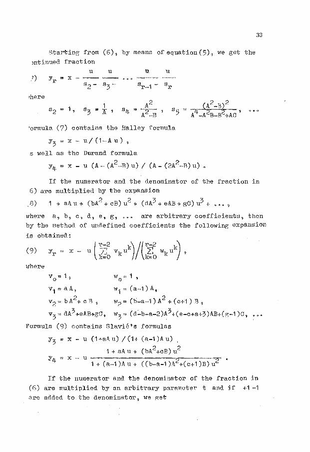
Startine; from (6), by means of equation (5), we get the )ntinued fraction
rhere
y = Xr
u u 11 u
33
... 'ormula (7) contains the Halley formula
y3 = x- u/(1-Au),
s well as the Durand formula
y4 = x - u (A- (A2..:B) u) I (A- (2A2-B) u) •
If the numerator and the denominator of the 6) are multiplied by the expansion
2 2 3 3 ,8) 1 + aAu+ (bA +CB)u + (dA +eAB+gC)u +
fraction in
e o o 9
where a, b, c, d, e, g, ••• are arbitrary coefficients, then by the method of undefined coefficients the following expansion
is obtained:
(9)
where
v 0"' 1'
v1 caA,
2 v2 =bA+cB,
v3
= dA3+eAB+gC,
wo = 1 '
w1 ::(a-1)A,
w2 = (l:i-a-1) A2 + (c+1) B,
w3 = (d..:b~a-2)-~3+(e-c+a+3)AB+(g-1 )C,
Formula (9) contains Slavic's formulas
y3 =x-u (1+aA.u)/(1+(a-1)Au)
1 + aA u + (bA2+cB) u2
y 4 "' X - U 1 + (a-1 )Au+ ((b-a-1 )A2+(c+1 )B) uz- •
If the numerator and the denominator of the fraction in (f>) are multiplied by an arbitrary parameter t and if +1 -1 Rre added to the denominator, we get
4
/(
. r::2 k \'1
y r "' x ,;.. t u ,t- 1 + ( 1 + J,;,;1
t qk u } ) •
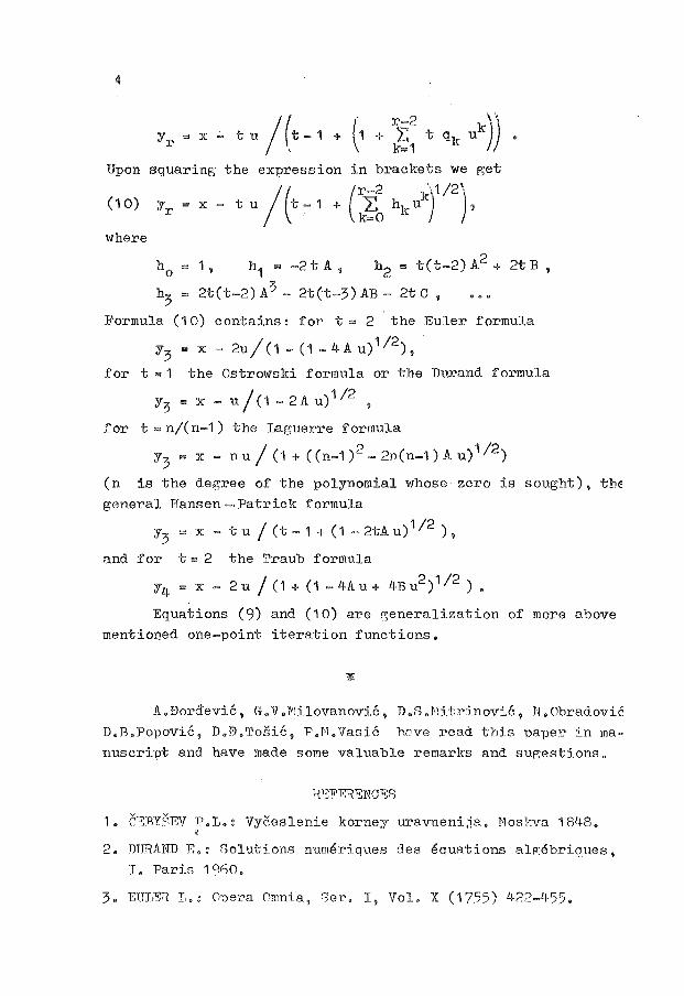
Upon squaring the expression in brackets we get
(i 0) Yr = X - t u I (t- 1 + (:t: hk ukr 12)'
where
2 h0
1, h; "'-2tA, b2 = t(t-2)A + 2tB,
h3
= 2t(t-2) A3- 2t(t-3) AB- 2t C ,
Formula (1 0) contains: for t = 2 the Euler formula
y3 = x- 2u/(1- (1-4A u) 112 ),
for t = 1 the Ostrowski formula or the Durand formula
y 3 = x - u / (1 - 2 A u) 112 ,
for t = n/(n-1) the Laguerre formula
Y3
"' x - n u / (1 + ( (n-1 ) 2 - 2n(n-1) Au) 1 /2)
(n is the degree of the polynomial whose zero is sought), thE
general Hansen-· Patrick formula
y3 = x- tu / (t-1 + (i -2tAu)112 ),
and for t = 2 the Traub formula
Y4 = x- 2u / (i + (i -4Au+ 4Bu2)1/2 ).
Equations (9) and (10) are generalization of more above
mentioned one-point iteration functions.
A.Dorctevic, G.V.JVfilovanovi6, D.S.l'~itrinovic, N.OhradoviC
D.B.Popovi6, D.D.Tosi6, P.r~.Vasi6 h2ve read. this paper in ma
nuscript and have made some valuable remarks and sugestions.
1. r-sBYP1W P.I .• : Vyceslenie korney uravneni,ia. l1osJ.:va 1848.
2. DTffiAND E.: Solutions numeriques des equations algebriques,
I. Paris 1960.
3. EULER I1.: 0Dera Omnia, Ser. I, Vol. X (1755) 422-455.

35
• HALI,EY E. : A new, exact and easy method of finding the roots of equations generally, and that without any previous reduction. Phil.Trans.Roy.Soc.London 18(1694-) 136-14-5.
5. HAMILTON H.J.: Roots of equations by functional iteration. Dul)e Math.J. 13(194·6) 113-121.
6. HANSEN E., PATRICK M.: A family of root finding methodse Numer.I-1ath. 27(1977) 257-269.
7. LAGUERRE E.N.: Sur une m~thode pour obtener par approximation les recines d'une ~quation alg~brique qui a toutes ses racines r~elles. Nouvelles Ann.de !1ath. 2e series 19(1880) 88-1 o;.
8., NEWTON I.: Letter to G.W.Leibniz, 13.6.1676.
9. OSTROl!lSKI A.: Solution of equations and systems of equations. New York 1960.
10. SLAVIC D.V.: Solution of equations by function modification, Univ.Beograd Publ.Elektrotehn.Fak.Ser.Mat.Fiz. N°735-762 ( 1 982) 127-129.
11. SLAVIC D.V.: The generalization of ten rational approximations of iteration functions. These publications.
12. TRAtffi J.F.: Iterative methods for the solution of equations, Englewood Cliffs 1964-.
13. WHITTAKER E.T.: A formula for the solution of algebraic or transcendental equations. Proc.Edinburgh Math.Soc. 36(1918) 103-106.

I
I
I
I
I
I
I
I
I
I
I
I
Numerical Methods and
Approximation Theory
Nis, September 26-28, 1984
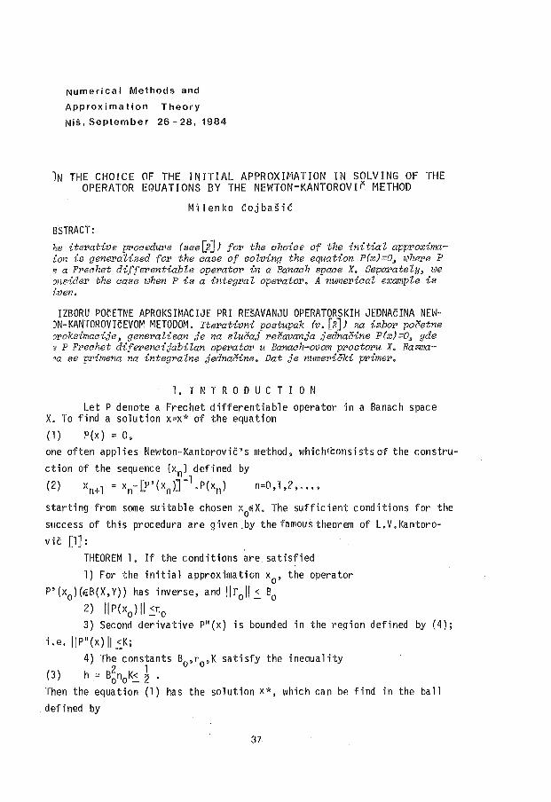
)N THE CHOICE OF THE INITIAL APPROXIMATION IN SOLVING OF THE OPERATOR EQUATIONS BY THE NEWTON-KANTOROVI~ METHOD
Milenko Cojbasic
BSTRACT:
he iterative procedure (see [2]) for the choice of the initial approximaion is generalized for the aase of solving the equation P(x)=O, where P s a Freahet differentiable operator in a Banach space X. Separately, we ?nsider the case when P is a integral operator. A numerical example is Z:ven.
IZBORU POcETNE APROKSI~1ACIJE PRI REsAVANdU OPERATORSKIH JEDNAciNA NEWJN-KANTOROVIcEVOM METODOM. Iterativni postupak (v. [2]J za izbor pocetne ?roksimacije, generaZisan je na slucaj resavanja jednacine P(x)=03 gde ~ P Freahet diferencijabilan operator u Banach-ovom prostoru X. Razmaoa se primena na integralne jednacine. Dat je numericki primer.
1. INTRODUCTION
Let P denote a Frechet differentiable operator in a Banach space X. To find a solution x=x* of the equation
(1) P(x) = 0,
one often applies Newton-Kantorovic's method, whichli::onsists of the constru
ction of the sequence {xn} defined by
(2) xn+l = xn-[p'(xn)r1.P(xn) n=O,l ,2, ... ,
starting from some suitable chosen x0EX. The sufficient conditions for the
success of this procedura are given by thefamoustheorem of L.V.Kantoro
vic [1]:
THEOREM 1. If the conditions are satisfied
1) For the initial approximation x0
, the operator
P' (x0
) (E:B(X, V)) has inverse, and llr 0
!1 .2_ B0
2) II P ( x0
) II .2_n0
3) Second derivative P"(x) is bounded in the re(jion defined by (4);
i.e. IIP"(x)II.2_K; 4) The constants B
0,n
0,K satisfy the inequality
2 1 (3) h = B0n0 K.2_ 2 Then the equation (1) has the solution X*, which can be find in the ball
defined by
37
B
l-lf.:21l (4) llx-x0 II.:_N(h0 ).n0 = h 0 .n0
0
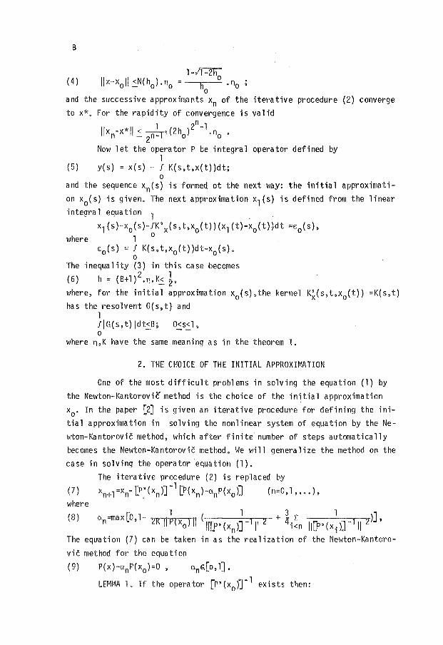
and the successive approximants xn of the iterative procedure (2) converge to x*. For the rapidity of convergence is valid
n llxn-x*ll.:_ ~d2h0 ) 2 -l .n
0 •
2 Now let the operator P be integral operator defined by
1 (5) y(s) = x(s)- f K(s,t,x(t))dt;
0
and the sequence xn(s) is formed ot the next way: the initial approximati-on x
0(s) is given. The next approximation x1(s) is defined from the linear
integral equation 1 x1 (s)-x
0(s)-JK' x(s, t,x
0(t)) (x1 (t)-x
0(t))dt =£
0(s),
where 1 ° £ 0 (s) = f K(s,t,x
0(t))dt-x
0(s),
0 The inequality (3) in this case becomes
2 1 ( 6) h = ( B+ 1 ) • n. v~ 2, where, for the initial approximation x
0(s),the kernel K~(s,t,x0 (t)) =K(s,t)
has the resolvent G(s,t) and 1 flG(s,t)ldt<B; 02s.:_l, 0 -
where n,K have the same meaning as in the theorem 1.
2, THE CHOICE OF THE INITIAL APPROXIMATION
One of the most difficult problems in solving the equation (1) by the Newton-Kantorovic method is the choice of the initial approximation x
0• In the paper [2] is given an iterative procedure for defining the ini
tial approximation in solving the nonlinear system of equation by the Newton-Kantorovic method, which after finite' number of steps automatically becomes the Newton-Kantorovic method. We ~till genera 1 ize the method on the case in solving the operator equation (1),
The iterative procedure (2) is replaced by
(7) xn+l =xn- [P~ (xn)J -1
[P(xn) -anP(x0)] (n=O, 1, ••• ), where (s) [o 1 1 ( 1 3 1 l].
an=max '- 2K IIP(xolll -,j[p•(xn)r1112 + l[i~n li[P'(xi)rlll2
The equation (7) can be taken in as the realization of the Newton-Kantorovic method for the equation (9) P(x)-anP(x0 )=0 , anc;.[o, 1],
LEMt~A 1. If the operator rr•(x0)T 1 exists then:
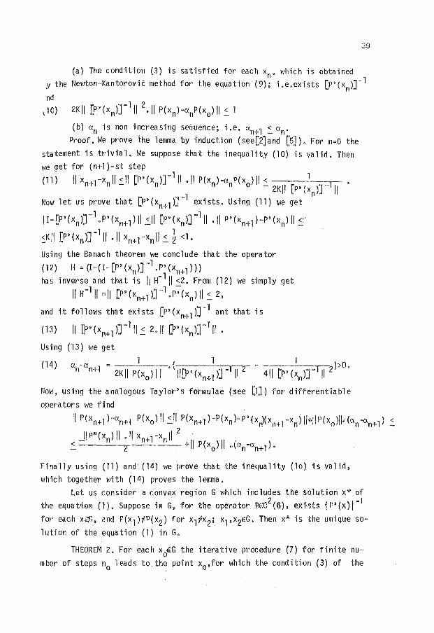
39
(a) The condition (3) is satisfied for each x , which is obtained n y the Ne~rton-Kantorovic method for the equation (9); i .e.exists [P' (xnlT 1
nd
1 10) 2KII [P• (xn)r 1
11 2
.11 P(xn)-anP(x0
) II:::_ 1
{b) an is non increasing seauence; i.e. an+l :::_an.
Proof. ll/e prove the lemma by induction (see[2Jand [5]). For n=O the
statement is trivial. We suppose that the inequality {10) is valid. Then
we get for (n+l)-st step
(11) II xn+l-xnll.::ll (P'(xn)r1
11 .11 P(xn)-anP(x0 )11 < 1 -:.,-;:--. - 2KII [P'(xn)] II
Now let us prove that [P'(xn+l)r1 exists. Using {ll) we get
II-[P'(xn)r1
.P'(xn+llll.::ll [P'(xn)r1
11.11 P'(xn+l)-P'(xnlll_::i:
::KI! [P'(xn)J-111 .IJ xn+l-xnll :::_ ~ <1.
Using the Banach theorem we conclude that the operator
( 12) H = (I- ( I- [P' ( xn)] -l • P' ( xn+ 1 ) ) )
has inverse and that is II H- 1 11 <2. From (12) ~1e simply get
II H-111 =II [P'(xn+l)rl.r-;-(xn)ll :::_ 2,
and it follows that exists [P'(xn+l)r1 ant that is
(13) II [P'(xn+llT1
11.:: 2.11 !J''<xn)r1
11.
· Using (13) we get
( 14) 1 ( 1 _ I )>O. an-an+l = 2KII P(xo)ll. II[P'(xn+l)rlll2 411 [P'(xn)rlll2
Now, using the analogous Taylor's formulae (see (lJ) for differentiable
operators we find
!I P(xn+l)-an+l P(x0 )11 :::_11 P(xn+l)-P(xn)-P'(xJ(xn+l-xn)II+;JP(x0 )l~(an-an+l) _2
JIP"(xn)ll.ll xn+l-xn112 . < -·----+II P(xo)ll •. (an-an+l).
Finally using (11) and (14) we prove that the inequality (lo) is valid,
~1hich together 1~i th ( 14) proves the 1 emma.
Let us consider a convex region G which includes the solution x* of
the e6]uaHor-1 (1), Suppose il!l G. for the opi>!rator Pt:C2(G), exi·sts ·IP'{x)l-l
fm· each xift, and P(x 1);-!P(x2) for x1;-!x 2; x1,x2EG. Then x* is the unique so
lution of the equation (1) in G.
THEOREM 2. For each xo'.G the iterative procedure (7) for finite nu
mber of steps n0
Teads to the point x0
,for which the condition (3) of the
m:!wton-Kantorovic method is satisfied, and an=O, for n~n0 •
l'roof. We first prove that the sequence!! [P'(x )rl11 Is bounded, \1le l n
suppose the opposite; i.e. that II [P• (xn)r 11-+=,n-roo, By the lemma
an4a ~ [o, 1], then by {10) P(xn)4aP(x0). From the definition of the region
G and characteristics of mapping P, we conclude that P{G) is a convex re
gion, P{x0
)EiP{G) and P{x*)=OEiP{G). Therefore is aP(x0
)EP{G). But then x = P-l (aP(x
0) )(iG,
and xn-+x. So
II [r• (xn)r111-+ll [P• (x)T.111-+<» ,
which is in contradiction with assumption. Thus II [P'(xn)]-1 11 ::_L<oo, Using
{8) and the lemma we get that for
n :_no:. (2KL2 1! P{x
0) II -1),
O'.n = 0 and the condition for a pp 1 yi ng the Newton -Ka ntorov i c method is sa
tisfied.
NOTE l. In the paper [2] is considered the case when P is the system
of nonlinear equations.
We suppose that for the integral equation (5) the condition {6) is
not satisfied. Using the lemma 1 for defining the initial approximation we
and Gn{s,t) is the resolvent of the integral equation with the kernel
K~{s,t,xn(t)), Using theorem 2 the successive approximative \'Jhich are get
by solving the linear integral equation (15) lead to xn for which is the
condition {6) for applying the Newton.-Kantorovii' method ~s satisfied.
( 18)
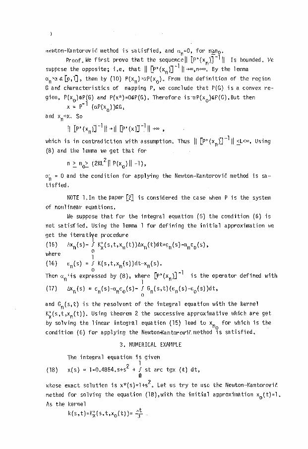
3. NUJVIERICAL EXJlJ1PLE
The inte~ral equation is given 2 1
x(s) = l-0.4854.s+s + ! st arc tgx (t) dt, a
11hose exact solution is x*(s)=l+s2• Let us try to use the Newton-Kantorovic
method for solving the equation ( 18), with the i nitia 1 approximation x0
( t) = 1.
1\s the kernel
k{s,t)=Kx(s,t,x0 {t))= ~,

1 s ueyenera ted, according [3] a resolvent can be find from the integra 1 equation for a reso1vent,and we get
3 G(s,t) = S.st.
Using (16) and the estimation for K(see [4] ), we can find B,n,K,h0
1 3 B =max !IG(s,t)idt = 1U' n= max~0 (s)i= 0,9073,
s 0 s
K =max IK 11
2(s,t,u)l= 0,6495, h0=(B+1) 2nK=0,9959>~. s, t u
So, we can not use the Newton-Kantorovic method. Let us apply the iterative procedure (15) for defining the initial approximation. We easily get a
0=0,4979, By solving the i.ntegra 1 equation (15) for n = 0 we get
2 ~x0 (s)=0,5021 s +0,0195s; x 1 (s)=x 0(s)+~x0(s)=
= l+0.0195s + 0,5021 s2,
Likely for x1 (s) ~1e define the constants n1 and B1 :n1=0,4416, s1=0,2222
(see[5}), Now it is 2 1 h1 = (B1+1) n1.K=0,4284< 2 •
41
So, the condition for using the Nev~on-Kantorovic method with the initial approximation x1(s)=l+O,Ol95,s + 0,502l,s2, is satisfied, For the next iteration we get
2 2 ~x 1 (s) = 0,4979 s -O,Ol35,s; x2(s) = x 1 (s)+~x 1 (s)=s +l+0,0060,s.
Since the exact solution is x*(s)=l+s2, that is the maximal error
maxlx*(s)-x2(s)i= ma~0,006.sl= 0,06<10-2 • s s
NOTE 2, In the paper [4] for x0
(s) =~one obtains h0=0,451<0,5 so
it is possible to use the Newton-Kantorovic method inmediatelly. Here x1(s)=s 2+0,0067 s+l.
REFER EN C E.S
1. KANTOROVIc L.V.: Funkcional'nyj analiz i prikladnaja matematika. Uspehi Mat.Nauk, 3(1948), 89-185,
2. KUL'ciCKIJ o,JU., siMELEVIc L.I.: 0 nahozdenii nacal'nogo priblizenija dlja metOda Newtona. L,Vycisl. Mat. i Mat. Fiz, 14{1974),1016-1018.
3. KRASNOV M,L.: Integra1'nye uravnenija, Moskva,l975. 4. ZAGADSKIJ D.M.: Priblizennoe resenie nelinejnyh integral'nyh uravnenij,,
Ph. thesis, Pedag, inst. im. A. I.Gercena, Leningrad, 1946, 5, COJBAsic M,M.: Neki aspekti primene Newton-Kantoroviceve metode, Mr.
thesis, PMF Beograd, 1982.

I
I

Numerical Methods and
Approximation Theory
Nis. September 26-28, 1984
NUMERICAL SOLUTION OF THE FREDHOLM INTEGRAL EQUATION OF
THE FIRST KIND WITH LOGARITHMIC SINGULARITY IN THE KERNEL
Tomaz Slivnik, Gabrijel Tomsic
ABSTRACT:
The paper describes a numerical method for the solution of
the Fredholm integral equation of the first kind with loga;;
rithmic singularity in the kernel. The method is based on
proper substitution for the singularity and on the use of
generalized quadrature formulas which allow a faster con-
vegence.
NUMERICNA RE~ITEV FREDHOLMOVE INTEGRALSKE ENACBE PRVE VRSTE Z LOGARITMICNO SINGULARNOSTJO V JEDRU. v dlanku je opisana
numeridna metoda za resitev Fredholmove integralske enacbe
z logaritmidno singularnostjo v jedru. V metodi je uporab
ljena posebna substitucija in posplosene kvadraturne formu
le, ki omogodajo hitro konvergenco.
1. INTRODUCTION
The solutions of electrostatic problems can be often
formulated by the Fredholm integral equations of the first
kind. For instance the charge distribution 0 (x) on the sur-
face of the microstrip transmission line is given in the
following form
43
I
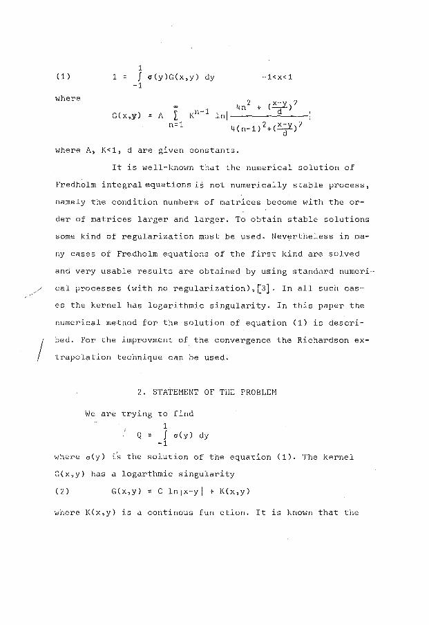
( 1)
where
1 1 = f a(y)G(x,y) dy
-1 -1<x<1
G(x,y) = A L 4n2 + (x~y)2
Kn-1 ln l-----==----n=1 4(n-1)2+(~)2
d
where A, 1<<1, d are given constants.
It is well-known that the numerical solution of
Fredholm integral equations is not numerically stable process,
namely the condition numbers of matrices become with the or-
der of matrices larger and larger. To obtain stable solutions
some kind of regularization must be used. Nevertheless in rna-
ny cases of Fredholm equations of the first kind are solved
and very usable results are obtained by uaing standard numeri
cal processes (with no regularization),[3}. In all such cas
es the kernel has logarithmic singularity. In this paper the
numerical method for the solution of equation (1) is descri-
bed. For the improvment of the convergence the Richardson ex-
trapolation technique can be used.
2. STATEMENT OF THE PROBLEH
We are trying to find
1 Q = f a(y) dy
-1
where a(y) i's the solution of the equation ( 1). The kernel
G(x,y) has a logarthmic singularity
( 2 ) G(x,y) = C lnlx-yJ + K(x,y)
where K(x,y) is a continous fun ction. It is known that the
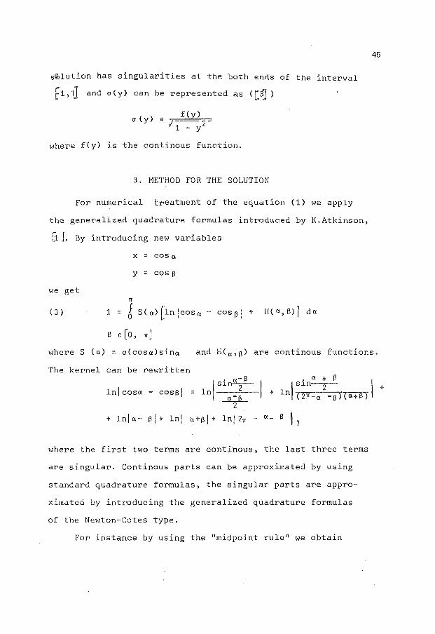
s~lution has singularities at the both ends of the interval
f1,1] and a(y) can be represented as <[3J)
a (y) = f(y) .; 2--1 - y
where f(y) is the continous function.
3. METHOD FOR THE SOLUTION
For numerical t~eatment of the equation (1) we apply
the generalized quadrature formulas introduced by K.Atkinson,
~]. By introducing new variables
X = COS a
y = cos fl
we get 1T
( 3) 1 = 6 S(a)[lnlcosa- cos 8 1 + H(a,f3)] da
fl e: [a, 11]
45
where S (a) = a(cosa)sina and H(a,fl) are continous functions.
The kernel can be rewritten
lnlcosa- cosel
a-fl = lnl sin-2- I +
--lL.1L.. 2
+ lnla- fll + lnl a+fll + ln/211 - a_ fl \ j
where the first two terms are conti'nous, the last three terms
are singular. Continous parts can be approximated by using
standard quadrature formulas, the singular parts are appro-
ximated by introducing the generalized quadrature formulas
of the Newton-Cotes type.
For instance by using the "midpoint rule" we obtain
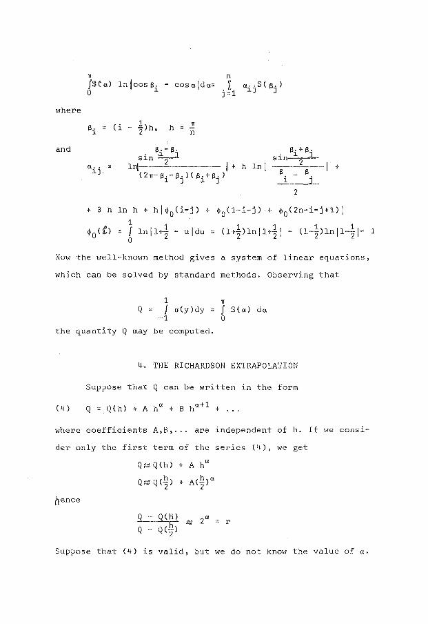
where
and
TI n f'Sta.) lnjcos fl. - cosa.ldex= L a· .S( fl·) 0 l j=1 l] J
l h ::: TI fli=(i-2)h, n
Ct. • = l]
. ~i- flj s1n 2
1 1 + h ln 1 ( 2 n- fl.- fl. ) ( fl. + fl. )
l J l J
fl· +fl. sin 1 J
2 -fl-~fl--1 +
i j
2
+ 3 h ln h + hi$ 0Ci-j) + $0(1-i-j) + ~ 0 (2n-i-j+1)1 1! 1 1 1 1 1 $0 Cl) = 0
lnll+2 - u!du = (l+2 )lnll+2 1 - (l-2 )lnll-2 !- 1
Now the well-known method gives a system of linear equations,
which can be solved by standard methods. Observing that
1 TI
Q = J a(y)dy = J S(o.) da -1 0
the quantity Q may be computed.
4. THE RICHARDSON EXTRAPOLATION
Suppose that Q can be written in the form
(4) Q = Q(h) +A hex+ B ha+ 1 + ...
where coefficients A,B, ••. are independent of h. If we consi-
der only the first term of the series ( 4) ) we get
Q;:::: Q(h) + A ha
Q;:::: Q (~) + A(.!!)a 2
hence
Q - Q (l-i) 2ex Q(.!!)
I;;: = r Q - 2
Suppose that (4) is valid, but we do not know the value of ex.
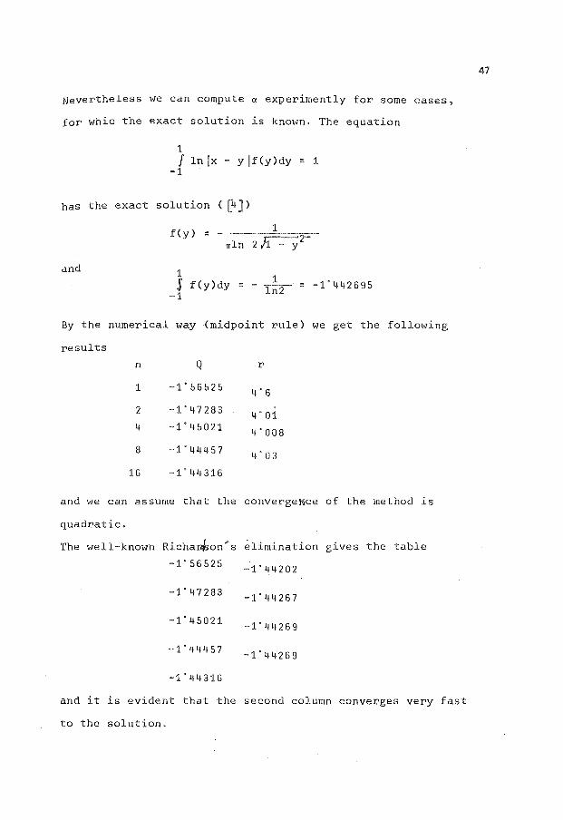
Nevertheless we can compute a experimently for some cases,
for whic the exact solution is known. The equation
1 J lnlx- y if(y)dy = 1
-1
has the exact solution ( ~])
and
f(y) = -rrln 2
1 s f(y)dy = -1
= -1'442695
By the numerical way (midpoint rule) we get the following
results
n Q r
1 -1'56525 4'6
2 -1'47283 4'01 4 -1'45021 4'008
8 -1'44457 4'03
16 -1'44316
and we can assume that the convergeMce of the method is
quadratic.
The well-known Richa~on~s elimination gives the table
-1'56525 -1'44202
-1'47283 -1'44267
-1'45021 -1'44269
-1'44457 -1'44269
-1'44316
and it is evident that the second column converges very fast
to the solution.
47
We compute extensive tables of Q for the different
values of constants K and d. When using, for instance._ge
neralized Simpson~s rule, the four point approximation com
pletely agrees with the results which can be find in the li
terature, [2] .
REFERENCES
[1] ATKINSON K.E.: Extension of th~ Nystr5m method for the
numerical solution of linear integral equations of the
second kind, MRC Report, 1966
[2] SILVESTER P.: TEM wave properties of microstrip trans
mission lines, Proc.IEEE London, vol.115,No.1, 1968
[3] SILVESTER P., BENEDEK P.: Electrostatic of the Microstrip
Revisited, IEEE Trans, on MTT, Nov. 1972
[4] STAKGOLD I.: Boundary Value Problems of Mathematical
Physics, MacMillan Co., New York, 1968

Numerical Methods and
Approximation Theory
Nis, September 26-28, 1984
ON A CLASS OF COMPLEX POLYNOMIALS HAVING All ZEROS IN A HALF DISC
WALTER GAUTSCHI AND GRADIMIR V. MILOVANOVIC
1\BSTRACT:
ve study the location of the zeros of the polynomial pn (z) = rrn (z) -
. i e rr (z), where {rrk} is a system of monic polynomials orthogo-n- 1 n- 1
rat with respect to an even weight function on (-a,a),
:s a real constant. We show that aU zeros of pn Ue
0 <a < oo, and e n-1 in the upper ha Zf
lise lzl <a 1\ Im z > 0, if 0 < 8 < rr (a)/rr 1 (a), and in the lower n-1 n n-!alf disc I z I <a 1\ Im z < 0, if -rr (a) /rr 1 (a) < e 1 < 0. The uUrasph-n n- n-rical weight function is considered as an example.
0 I<LASIKOMPLEKSNIH POLINOMA KOJIIMAJU SVE NULE U POLUI<RUGU.U radu se raz-
matra pr•oblem Zokalizac-ije nuZa polinoma p (z) = rr (z) - ie 1rr (z), n n n- n-1 gde je {rrk} sistem monianih poZinoma ortogonalnih u odnosu na parnu te-
zinslw funlwiju na (-a, a), 0 <a< oo, a en-l reaZna lwnstanta. Dokazujemo
da sve nuZe polinoma p Zeze u gornjem poZulwugu I z I< a 1\ Im z > 0 , ako n
je 0 < e 1
< rr (a)/rr (a), a u donjem polukrugu lzl <a 1\ Im z < 0, ako n- n n-1
je -rr (a) /rr 1
(a) < e_, < 0. Kao primer razmatrana je uUrasferna te-n n- n-l
Zinska funlwija.
1.1NTRODUCTION
In a series of papers, Specht C2J studied the location
of the zeros of polynomials expressed as linear combinations
of orthogonal polynomials. He obtained various bounds for the
modulus of the imaginary part of an arbitrary zero in terms
of the expansion coefficients and certain quantities depending
only on the respective orthogonal polynomials. Giroux ClJ
sharpened some of these results by providing bounds for the
sum of the moduli of the imaginary parts of all zeros. In the
prooess of doing so, he also stated as a corollary the follo
wing result.
49
0
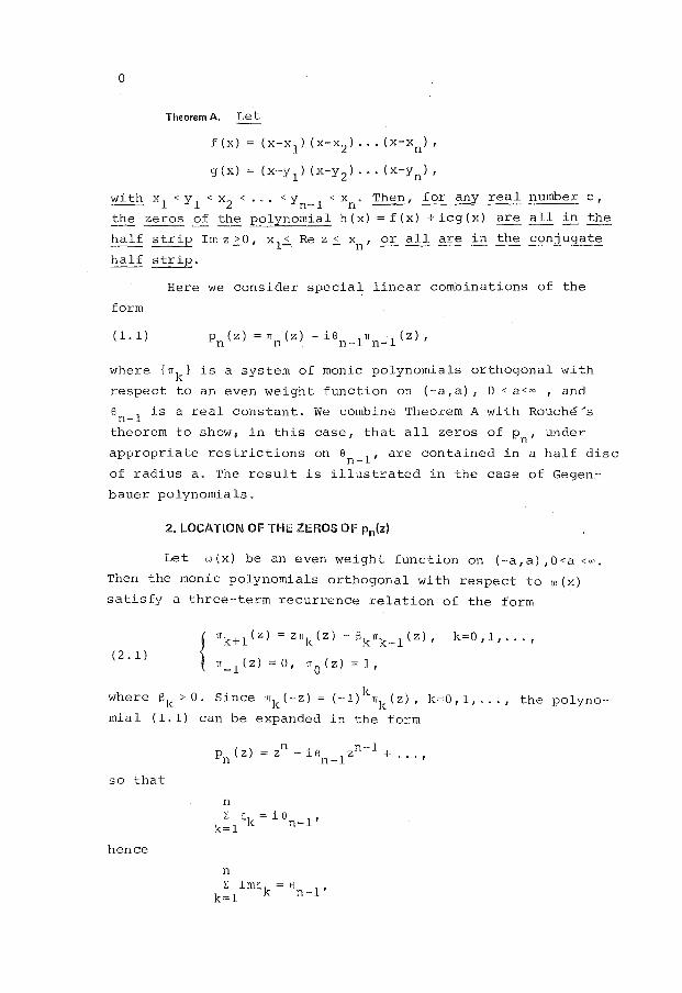
Theorem A. Let
f (x)
g(x)
(x-x1
) (x-x2 ) ... (x-xn),
(x-y1) (x-y2) ... (x-yn),
with x 1 <y 1 <x2 < ••• <yn_ 1 <xn. ~'for any real number c,
the~ of the polynomial h(x) =f(x) +icg(x) are all in the
half strip Im z ,;::.o, x 1~ Re z ~ xn, 9E all ~ in the conjugate
half strip.
Here we consider special linear combinations of the
form
( l. 1) p (z) =rr (z) -ie 1rr .1 (z), n n n- n-
where {rrk} is a system of monic polynomials orthogonal with
respect to an even weight function on (-a,a), 0 < a<oo , and
en_ 1 is a real constant. We combine Theorem A with Rouche/s
theorem to show, in this case, that all zeros of pn, under
appropriate restrictions on en_ 1 , are contained in a half disc
of radius a. The result is illustrated in the case of Gegen.
bauer polynomials.
2. LOCATION OF THE ZEROS OF Pnh:)
Let w(x) be an even weight function on (-a,a) ,O<a <oo,
Then the monic polynomials orthogonal with respect to w(x)
satisfy a three-term recurrence relation of the form
(2. 1) {
rrk+ 1 (z) = zrrk(z)- i3krrk_ 1 (z),
rr_ 1 (z)=O, rr0
(z)=1,
k=O, 1, ... ,
where Sk > 0. Since rrk(-z) = (-1)krrk(z), k=0,1, ... , the polyno
mial (1.1) can be expanded in the form
so that
hence
p (z)=zn-ie 1zn- 1 +
n n-
n l: s
1 = i 8
1,
k=1 < n-
n
l: Im~;k = en-1, k=1
.... ,
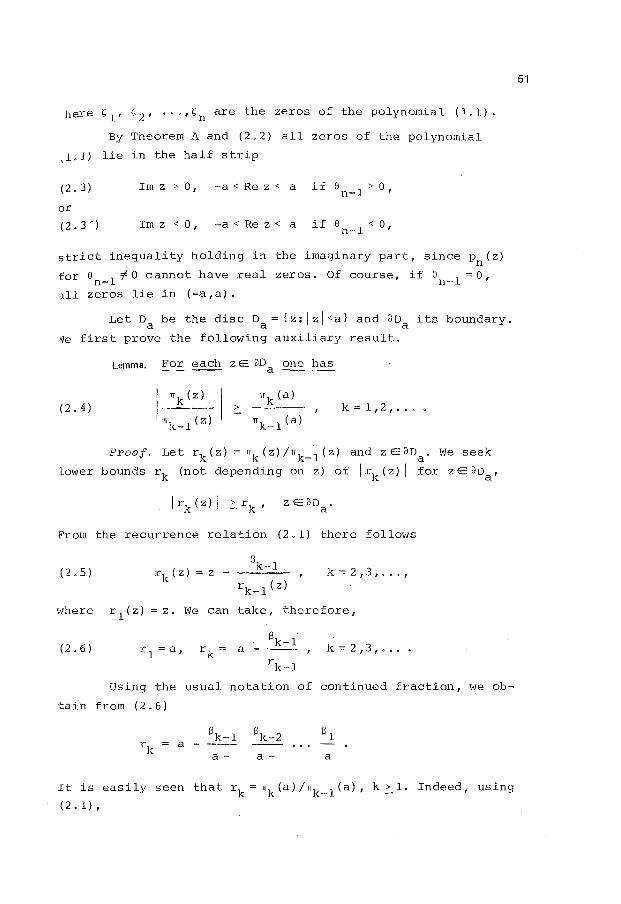
here s 1 , s 2 , ... ,snare the zeros of the polynomial (1.1).
By Theorem A and (2.2) all zeros of the polynomial
,1.1) lie in the half strip
(2. 3) I m z > 0 , -a < Re z < a if 8 n _1
> 0 ,
or
(2. 3 "') Imz <0, -a<Rez< a if en_ 1 <0,
strict inequality holding in the imaginary part, since pn(z)
for en_ 1 -=} 0 cannot have real zeros. Of course, if en_ 1 = 0,
~11 zeros lie in (-a,a).
Let D be the disc D = { z: I z I <a} and 3D its boundary. a a a qe first prove the following auxiliary result.
Lemma. For each z E 3D one has --- ---~ a ---
(2. 4) lrrk(z) I> rrk(a)
rrk-1 (z) rrk-1(a) k = 1,21 • • • •
Proof. Let rk ( z) = rrk (z) /rrk_ 1 ( z) and z E 3D a. We seek
lower bounds rk (not depending on z) of lrk(zll for zE3Da'
z E 3D . a
From the recurrence relation (2.1) there follows
(2. 5) rk(z)=z-rk-1 (z)
k=2,3, ... ,
where r 1 ( z) = z. We can take, therefore,
(2. 6) k=2,3, ...
rk-1
Using the usual notation of continued fraction, we ob
tain from ( 2. 6)
a -a- a- a
It is easily seen that rk = rrk (a) /rrk_ 1 (a), k ~ l. Indeed, using
( 2 • 1) 1
51
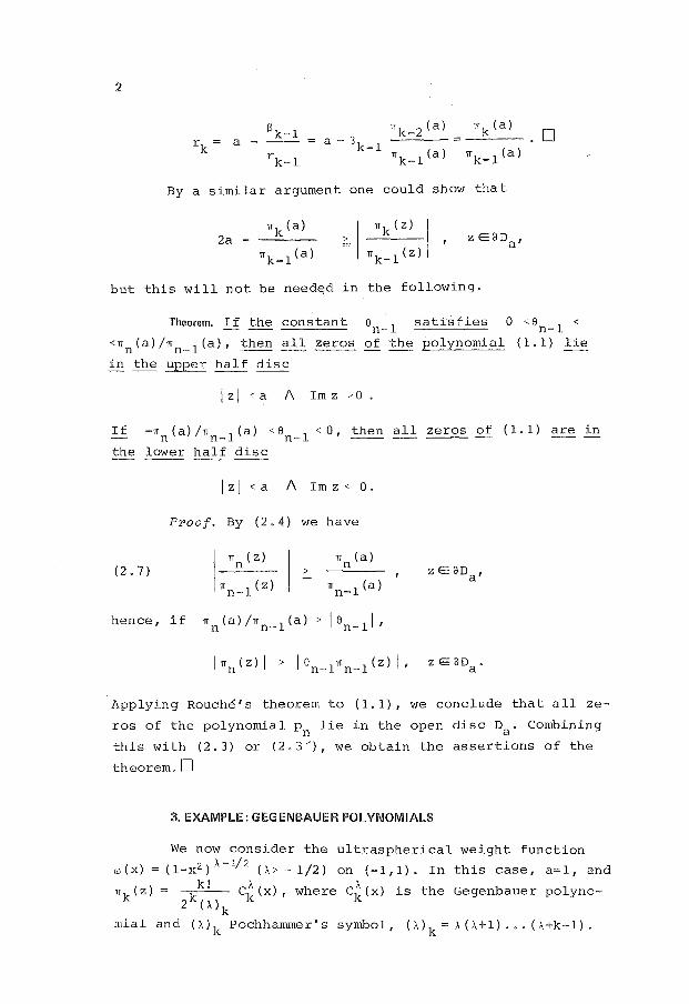
2
r = a -k
By a similar
2a -
13 k-1 1Tk-2 (a) a- sk-1
1Tk-1 (a) rk-1
argument one could show
1Tk(z) I 1Tk-1 (z) ,
1Tk (a)
1Tk-1 (a)
that
but this will not be needE:ld in the following.
D
Theorem. If the constant en_ 1 satisfies 0 <8n_ 1 <
<1ln(a)/1Tn_ 1 (a), then all zeros of the ~omial (1.1) lie
in the ~ half disc
I z I c a 1\ Im z _, 0 •
If -Tin (a) /1ln_ 1 (a) < en_ 1 < 0, then all ~ of ( 1.1) are in
the lower half disc
I z I < a 1\ Im z < 0 .
Proof. By (2.4) we have
11! ( z)
I
1Tn(a) (2. 7)
1Tn:1 (z) >
1Tn-1 (a)
hence, if 1T (a) /TI 1 (a) n n- > I en-11 ,
zE:lDa'
z E:lD . a
Applying Rouche's theorem to (1.1}, we conclude that all ze
ros of the polynomial pn lie in the open disc Da. Combining
this with (2.3) or (2.3'), we obtain the assertions of the
theorem. D
3. EXAMPLE: GEGENBAUER POLYNOMIALS
We now consider the ultraspherical weight function
w(x) = (1-x2 ) A.-1/z (A.>- 1/2) on (-1,1). In this case, a=1, and
1lk(z) = Jk! c1"(x), where c
1"(x) is the Gegenbauer polyno-
2 <::(A) <:: <:: k
mial and (A.)k Pochhammer's symbol, (A.)k = A.(A+1) ... (Hk-1).

Since
2 (Hk-1)
md
c~ (1)
\ ck-1 (1)
2Hk-1
2 (Hk-1)
m~k 1
1here D is the di ff_erentiatio_n operator, our theorem implies
:he following
53
Corollary. Let denote the monic Gegenbauer poly-
tomial of degree k ~ parameter \. If the constant en_ 1 sa-2\+n-1 .
:isfies 0 < en_ 1 < , then all ~ of the polynom1al 2 (Hn-1)
)n(z) = 1T (z) -ie 1 11 1 (z) and of its derivatives lie in the n n- n-
~pper half disc I z I <1 1\ Im z >0. If - 2 \+n- 1 < e < 0 I then 2 ( Hn-1) n- 1
they ~ all in the lower half disc I zl <1 1\ Im z <0.
The upper bound (2Hn-1)/(2(A+n-1)) forle 1
1 becomes n-
n/(2n-l) in the case of Legendre polynomials (\=1/2), and 1/2
in the case of Chebyshev polynom~als (\=0).
REFERENCES
1. GIROUX A.: Estimates for the imaginary parts of the zeros
of a polynomial. Proc. Amer. Math .. Soc. 44(1974) 1 61-67.
2. SPECHT W.: Die Lage der Nu'llstellen eines Polynomes,I- IV.
Math. Nachr. 15(1956), 353-374; 1'6(1957), 257- 263; 16
(1957), 369-389: 21(1960), 201-222.

I
I
I
I
I
I
I
I
I
I
I
I
NU'"~rical Methods and
Approximation Theory •I
Nis, September 26-28, 1984
ON THE OPTIMAL CIRCULAR CENTERED FORM
Ljiljana D. Petkovid
.BSTRACT:
ome including circular appro:1v-imations of the closed set {f( z) : z E Z} f is a closed complex function and Z = {a; r} is a disk) in the oenered form {f( a) ; R} are considered in this paper. The optimal oenteed form {f( a) ; Ro}, where Ro = max If( a) - f( z) I ( z E Z), is compared 0 the centered forms which use 'l'aylor s series. The optimal radius R0 s determined for some standard (library) functions.
1 OPTI MALNOJ KRU'ZNOJ CENTRALNOJ FORM I. U ovom radu su razmatrae neke ukljui'Jujude kruzne aproksimacije zatvorenog skupa {f(z): z E Z} f je zatvorena kompleksna funkcija i Z = {c; r} je disk) u centraZnoj 'ormi {f( c); R}. Optimalna centralna forma {f( c) ; Ro}, gde je Ro ::::
.. ux If( c) - f( z) I ( z E Z) • uporedjena je sa centralnim formama koje koriste Taylorov red. Za neke standardne (bibl.iotecl<e) funkoije odredjen je optimalni radijus R0 .
Let Z = {w: lw-zl _:_r} = {z; r} (z EC, r;;:OO) be a disk with the
center z and the radius r. The set of all disks v1ill be denoted with
K(C). Let f be a complex valued function of a complex variable, anali
tical on the union of all disks which belong to the set U =K(C), such
that the set
f*(Z) = {f(z) :.zEZ} = U {f(z)} ZEZ
is closed for each Z E u1 = U. f*(Z) will be called the closed uni
ted extension of the function f ·over Z. Since the closed region f*(Z)
is not a disk in general, it is of interest ·for evaluation in circular
arithmetic to introduce a disk W vlhich includes the closed set f*(Z),
that is W = f* ( Z).
The circular region F(Z) such that the inclusion F(Z)= f*(Z)
holds for each ZEU 1 is the inclusive disl< for the range f*(Z). Cove··
ring of the exact range f*(Z) by the inclusive disk will be sometimes
called including approximation, or, shorter I-approximation. Obvi
ously. !-approximation is better if the quotient area { f*(Z)}/area{F(Z)}
is closer to 1.
55

In this paper we shall consider inclusive disks of the form F(Z)=
{ f(c); R} (Z= {c; r}). This form is centered and it will be shortly ca
lled the C-fol'm.
Among all inclusive disks with the C-form, the best !-approxima
tion is obtained by the disk with the radius
( 1) R = R0 = max If( z) - f{ c) I • Z E Z
The disk F0(Z) = {f{c) R0} is called the inclusive disk u.1ith the
optimal C-form.
Using computer programs, the special attention is dedicated to
the computation of standard (subroutine library) functions(ez, ln z,
arc tgz, sin z, cos z, zn, z 1/n). For some of these functions it is
possible to find the optimal radius R0 according to (1). In a such pro
cedure the following simple assertions, which we give without the proof,
wi 11 be used.
LEMMA 1: Let L be a closed region in complex plane. If there
exists WEL such that lf(r;JI =< lf(wJI for each i;EL then
max I f ( 1;) I ::: I f ( vJ) I . 1; E L
LEMMA 2: r[1]), p. 70). The inequality
lez -11 ~elzl- 1
is valid foY' arbitrary z E C.
LEMMA 3: Let u and v be real functions of a real variable
t E [a,b], and let f(t) =u(t) + iv(t). Iff is R-integrable
function, then b b
ljf(t)dtl ~ j1 f(tJ I dt.
a a LEMMA 4: {[4]. P· 370). If the condition ak ?~0 holds for
<A, then
for I z I <A.
Let r be the boundary of the disk Z= {c; r}, c= lcleiY and let
st = [o • 21!), P = TZI ·Then, an arbitrary point ZEr can be expressed by
z c + r e i 8 = c ( 1 + pe i w ) ( e ) ,wE Sl •
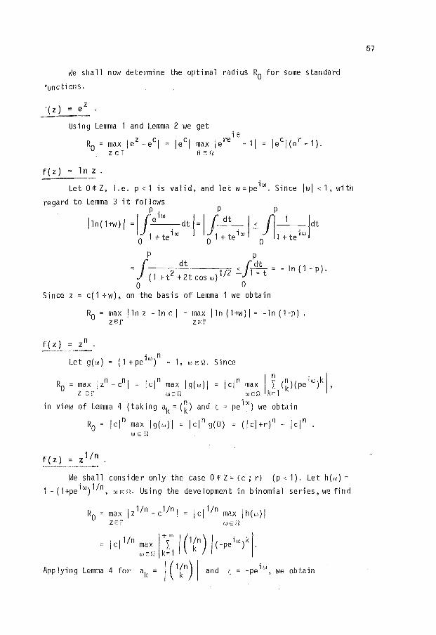
vie shall now determine the optimal radius R0
for some standard 0 uncti ons.
z z = e
Using Lemma 1 and Lemma 2 we get i e
R0
=max le 2 -ecl = lecl max lere -11 lecl(er -1). ZEf 8E~
f(z) = ln z.
1 i w Let O!J;Z, i.e. p<1 is valid, and et w=pe . Since lwl <1, with
regard to Lemma 3 it follows
/ln(1+w) / = lfpeiw dt I= I~~ I< flp 1 ldt 0 1 + te i w . 0 1 + te i w = 0 1 + te i w
p p
f dt (_dt = (1+t2 +2tcosw) 112 ~Jr:t= -ln( 1 -p).
0 0 Since z = c( 1 +w), on the basis of Lemma 1 we obtain
R0 =max llnz -lncl =max lln(1+w)l= -ln(1-p). ZEf ZEf
z . n
Let g(w) = (1 +pe 1w) - 1, uJE~. Since
R0 =max li -cnl = lcln max lg(w)l = lcln max I I (~)(peiw)k\, Z Ef WE~ WE~ k=1
in view of Lemma 4 (taking ak = (~) and ~ = pe iw) we obtain
n . · n n n R0 = lei max lg(w)l =lei g(O) (lcl+r) -lei
WE~
We shall consider only the case OiJ;Z={c;r} (p<1). Let h(w)=
1-(1+peiw) 1/n, wE~· Using the development in binomial series,wefind
R0
=max lz 1/n -c 11nl = lcl 1/n max lh(w)l ZEf WE~
= lcl1/n max j\oo /(1~n) 1(-peiw)kl· WE~ k=1
Applying Lemma 4 for ak = I ( 1 ~n) I and c; = -pe iw, we obtain
57
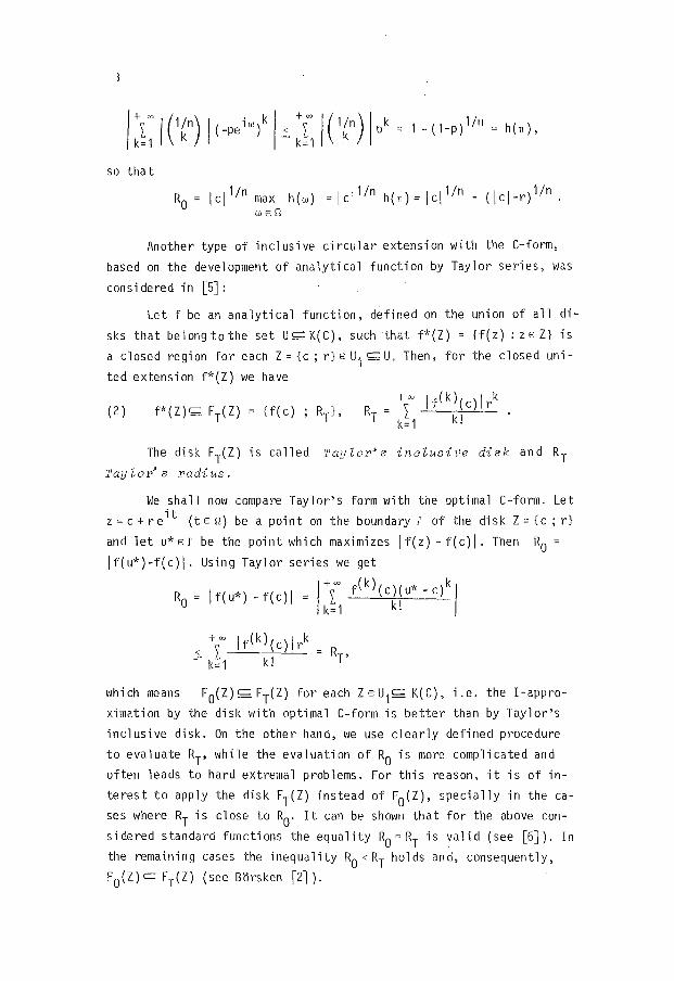
so that
R0
= lcll/n max h(w) = lcll/n h(n)= lcll/n- (lcl-r) 1/n. WEll
Another type of inclusive circular extension with the C-form,
based on the development of analytical function by Taylor series, was
considered in [5]:
Let f be an analytical function, defined on the union of all di
sks that belongtothe set U=K(C), such that f*(Z) = {f(z): ZEZ} is
a closed region for each Z = {c; r} E u1 = U. Then, for the closed uni
ted extension f*(Z) we have
+oo ( 2) {f(c) R = ~
T k=1
The disk FT(Z) is called Taylor's inclusive disk and RT
Taylor's radius.
We shall now compare Taylor's form with the optimal C-form. Let
z=c+reit (tEll) be a point on the boundaryr of the disk Z={c;r}
and let u*Ef be the point which maximizes lf(z) -f(c)l. Then R0 =
lf(u*)-f{c)l. Using Taylor series we get
Ro = If( u*) - f( c) I = I\"' f( k) (c)( u* - c) k / k=1 k!
+oo
~' ~ k=1
which means F0(z)= FT(Z) for each ZEU 1= K(C), i.e. the !-appro-
ximation by the disk with optimal C-form is better than by Taylor's
inclusive disk. On the other hand, we use clearly defined procedure
to evaluate RT' while the evaluation of R0 is more complicated and
often leads to hard extremal problems. For this reason, it is of in
terest to apply the disk FT(Z) instead of F0{Z), specially in the ca
ses where RT is close to R0. It can be shown that for the above con
sidered standard functions the equality R0 =RT is valid (see [6]). In
the remaining cases the inequality R0 < RT holds and, consequently,
F0{Z)c FT{Z) (see Borsken f2l ).

raylor's centered form (2) uses Taylor's development of an ana
ytical function f around the center c of domain Z = {c; r}. By expand
ng f(z) as Taylor's series around the origin (Maclaurin's series), we
1bta in
( 3)
In the sequel we shall use the following formula for the power of
a disk Z={c; r}
(4) zk = {c; r}k = {ck ; ( lcl+r/ -lclk},
which can be obtained from the definition for multiplication of two di
sks, introduced by Gargantini and Henrici [3].
Natural circular extension of (3) using (4) results in a circu
lar interval
F (Z) = I _i_~zk = I f 1
O) ck; I f {O)((Icl+r/-lclk) +oo (k) { +oo (k)( +ool (k) I }
p k=O k. k=O k. k=1 k!
( 5) F p ( Z ) = { f (c) ; Rp};;;;;;? { f ( z) ; z E Z} = f* ( Z ) ,
where
(6) +ool {k) I
R =I f (O)((Icl+r)k-lclk). p k=1 k!
The inclusive disk {5) will be called the power centered form.
According to the developing procedure it is normally to expect
that the power centered form is worse !-approximation for the exact
region f*( Z) than the Taylor's centered form. Thus, ~1e conjecture
(7) FT(Z) c: Fp(Z).
The inclusion (7) leads to an equivalent condition in the form of ine
quality RT~Rp, i.e.
+"'I (k)( I +"'I (k)( I ( 8) I f I c ) rk ~ I f I 0 ) ( ( I c I + r) k - I c I k ) .
k=1 k. k=1 k.
EXAMPLE 1. Let
n k q(z) = I akz (ak E C)
k=O
be a polynomial of degree n. On the basis of (2), (5) and (6) we find
Q ( Z) = { q (c) ; I .· I q ( k) (c) I rk } T k=1 k!
59

and
Op(Z) {q(c)
The inequality
~ I q ( k) ( c) I rk < I I ak I ( ( I c I + r) k ~ I c I k) k=1 k! = k=1
has been proved in [7]. which gives QT{Z)<=Qp{Z).
EXAMPLE 2, Let f(z) = ez and Z = {c ;.r} be arbitrary disk. Then
FT{Z) = {ec \ec\(er- 1)},
Fp{Z) = {ec el c\ (er -1)}.
Since \eel ~elc\ it follows FT(Z) <=Fp(Z) in the case of exponential
function.
The above examples confirm the conjecture (7), It is interesting that other considered examples also verify the inclusion (7). But, we are not able to prove the inequality (8) in general case {for arbitrary f) so that the conjectrure (7) remains as an open problem.
R E F E R E N C E S
1. ABRAMOWICZ M., STEGUN I.A.: Handbook of Mathematical Functions. New York 1965.'
2. BORSKEN N.C.: KompleiXJe Kreisstandardfunktionen. Freiburger IntervallBerichte 2( 1978).
3. GARGANTINI I .• HENRICI P.: Circular arithmetic and determination of
polynomial zeros. Numer. Math. 18 {1972), 305-320.
4. GARNIR H.G.: Fonctions de variables reelles I, Louvain-Paris 1963.
5. PETKOVIc L., PETKOVIC M.: The representation of complex circular
functions using Taylor series. ZAMM 61 (1981), 661-662.
6. PETKOVIC L.: 0 najboljim aproksimacijama zatvorenih oblasti pomocu
diskova. In: Proceedings of V Conference PPPR, Stubicke Toplice 1983, 83-88,
7. ROKNE J., WU T.: The circular complex centered form. Computing 28 ( 1982) ' 17 - 30.

Numerical Methods and
Approximation Theory
Nis, September 26-28, 1984
TWO METHODS FOR THE CURVE DRAWING IN THE PLANE
Dobrilo ~. Tosi6, Dejan v. Tosi6
ABSTRACT:
Two methods for the drawing of the curve, given by the equation F(x,y) = 0, are presented. The first method is based on a differential equation y' = -Fx/FY, which enables the the prediction of the next point of a given curve. The position of a predicted point is corrected. The second method has a random choice of the point with the same correction as in the first method. The corresponding program package TPLTS is realised in BASIC.
DVA METODA ZA CRTANJE KRIVIH U RAVNI. Data su dva metoda za crtanje krive date jednacinom F(x,y) = 0. Prvi metod je zasnovan na formiranju diferencijalne jednacine y' = -FxfFy' koja omogu6ava predikciju slede6e tacke krive. Polozaj ove tacke je korigovan. Drugi metod ima slucajni izbor tacke sa istom korekcijom kao o prvom metodu. Odgovaraju6i programski paket TPLTS realizovan je u BASICu.
1. INTRODUCTION
The curve tracing and curve drawing belongs to the classic exercise. Many papers and books are devoted to the qualitative curve representation (by searching of the characteristic points- particularly singular points), to the investigation of the behaviour of the curve in the neighbourhood those points, the position 'of asymptots, number of branches, etc. Thus we can draw a skech of the curve vrhich gives some approximation to the truth.
If the equation of the curve is given in an explicit or parametric form, then we have trivial case. The special case appears when the equation is presented in implicit form, i.e. F(x,y) = 0, where F is an differentiable function.
In the present paper we expose two methods for the curve drawing. This implies that the curve is to be drawn,
61
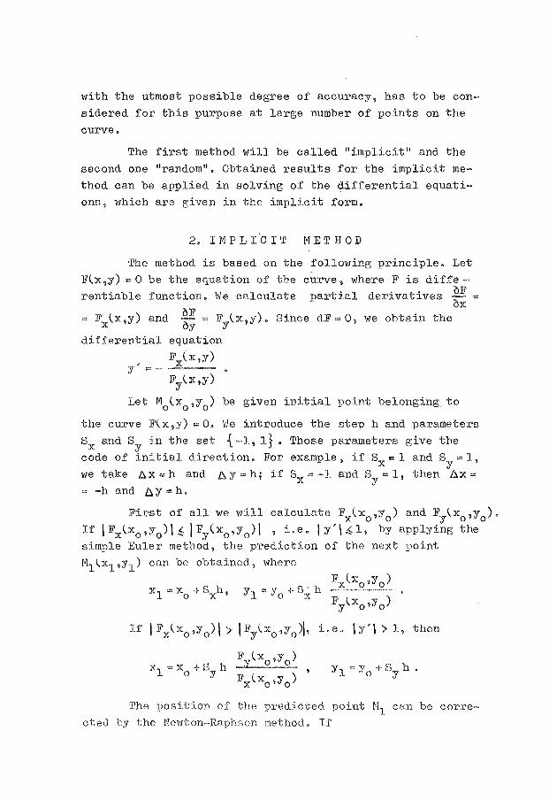
with the utmost possible degree of accuracy, has to be con
sidered for this purpose at large number of points on the
curve.
The first method will be called 11 implicit" and the
second one 11 random 11• Obtained results for the implicit me
thod can be applied in solving of the differential equati
ons, v1hich are given in the implicit form.
2. IMPLICIT METHOD
The method is based on the following principle. Let
F(x,y) = 0 be the equation of the curve, where F is diffe
rentiable function. We calculate partial derivatives ~! =
~F = F)x,y) and 'Oy = FY(x,y). Since dF"' 0, we obtain the
differential equation
,y)
Let M0(x
0,y
0) be given initial point belonging to
the curve F(x,y) = 0. vie introduce the step h and parameters
Sx and Sy in the set { -1, l} • Those parameters give the
code of in:.tial direction. For example, if Sx = 1 and Sy = 1,
we take Ax=h and D,y=h; ifSx=~l andS =1, then Ax= y = -h and D.Y =h.
First of all we will calculate Fx(x0
,y0
) and Fy\x0
,y0).
If \ Fx(x0
,y0
)\ ~I Fy(x0
,y0
)\ , i.e. I y'\~1, by applying the
simple Euler method, the prediction of the next point
M1(x1 ,y1 ) can be obtained, where
Fx(xo,yo)
FY(xo,yo)
If I Fx(x0
,y0
)\ > !Fy(x0
,y0
)!, i.e. \y'\ > 1, then
Fv\.xo,yo)
Fx\.xo,yo)
'J!he position of the predicted Doint l'\ can be corre
cted l'Y the Newton-Raphson method. If
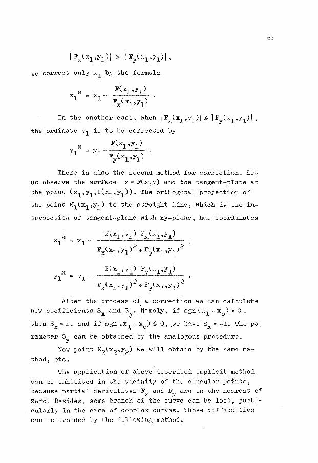
~e correct only x1 by the formula
F(xl,yl) xl * "' xl-
Fx(xl,yl)
In the another case, when I Fx(xl'yl) I~ l F/x1 ,y1 ) \,
the ordinate y1 is to be corrected by
F(xl ,yl) yl-
FY(xl,yl)
There is also the second method for correction. Let us observe the surface z = F(x,y) and the tangent-plane at the point (x1 ,y1 ,F(x1 ,y1 )). The orthogonal projection of
the point M1 (x1 ,y1 ) to the straight line, which is the in
tersection of tangent-plane with xy-plane, has coordinates
After the process of a correction we can calculate new coefficients Sx and sy. Namely, if sgn (x1 - x
0) > 0 ,
then Sx = 1, and if sgn (x1 - x0
) ~ 0, .we have Sx = -1. The pa
rameter Sy can be obtained by the analogous procedure.
Ne\v point M2(x2 ,y2) we will obtain by the same method, etc.
The application of above described implicit method can be iru1ibited in the vicinity of the sinp,ular points, because partial derivatives Fx and Fy are in the nearest of zero. Besides, some branch of the curve can be lost, particularly in the case of complex curves. Those difficulties can be avoided by the fdllowing method.
63
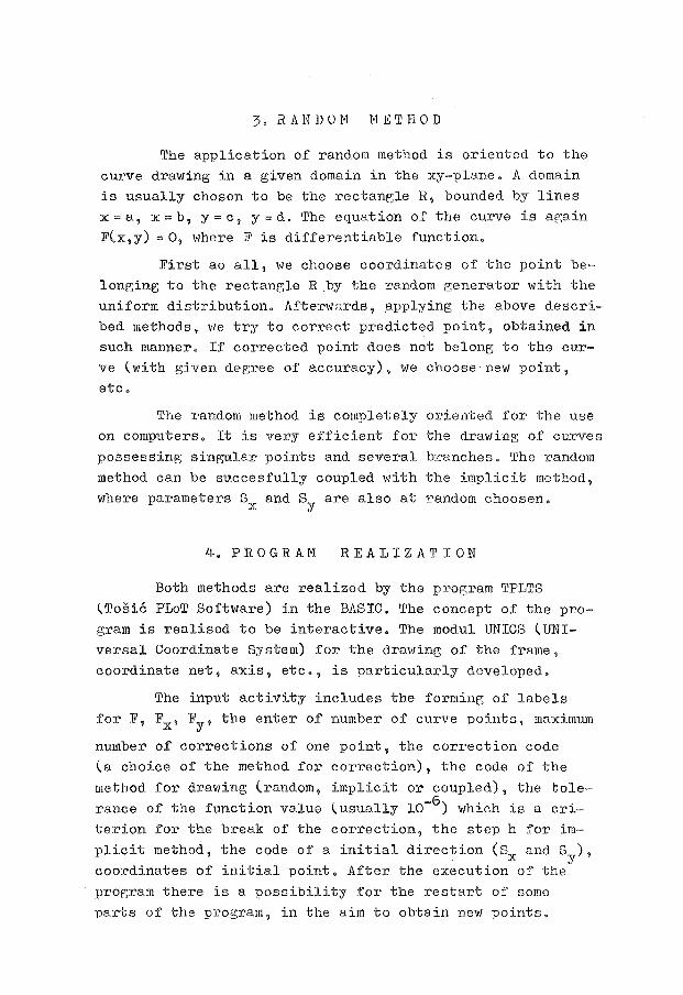
3, RANDOM METHOD
The application of random method is oriented to the curve drawing in a given domain in the xy-plane. A domain is usually chosen to be the rectangle R, bounded by lines x =a, x = b, y = c, y =d. The equation of the curve is again F(x,y) = o, where F is differentiable function.
First ao all, we choose coordinates of the point belonging to the rectangle R,by the random generator with the uniform distribution. AfterwRrds, ~pplying the above described methods, we try to correct predicted point, obtained in such manner. If corrected point does not belong to the curve (\'lith given degree of accuracy), we choose new point, etc.
The random method is completely oriented for the use on computers. It is very efficient for the drawing of curves possessing singular points and several branches. The random method can be succesfully coupled with the implicit method, where parameters Sx and Sy are also at random choosen,
4. PROGRAJ\1 REALIZATION
Both methods are realized by the program TPLTS \Tosic PLoT Software) in the BASIC. The concept of the program is realised to be interactive. The modul UNICS (UNIversal Coordinate System) for the drawing of the frame, coordinate net, axis, etc., is particularly developed.
The input activity includes the forming of labels for F, Fx, FY' the enter of number of curve points, maximum
number of corrections of one point, the correction code (a choice of the method for correction), the code of the method for dravling (random, implicit or coupled), the tolerance of the function value (usually l0-6 ) which is a criterion for the break of the correction, the step h for implicit method, the code of a initial direction (S and S ),
X y coordinates of initial point. After the execution of the program there is a possibility for the restart of some parts of the program, in the aim to obtain new points.
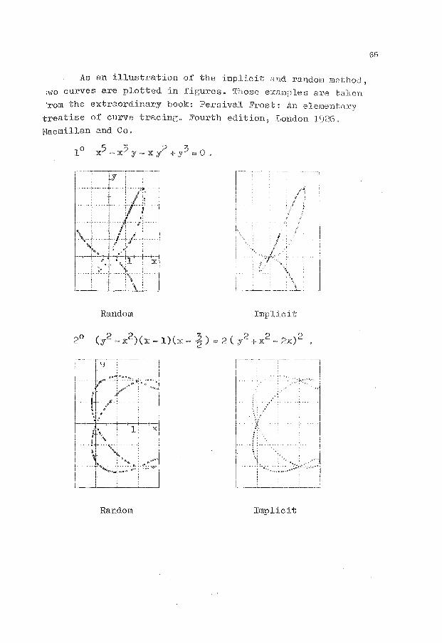
As an illustration of the implicit and random method, wo curves are plotted in figures. Those examples are taken ·rom the extraordinary book: Persival Frost: An element:C\ry
treatise of curve tracing. Fourth edition, I,ondon 1926 ..
jVJacmillan and Co.
1° x5 ~ x3 y ~ x y 2 + y3 = 0 ,
Random Imp lie it
Random Implicit
GG

I
I
Numerical Methods and
Approximation Theory
Nis, September 26-28, 1984
OPERATING WITH A SPARSE NORMAL EQUATIONS MATRIX
Brankica Cigrovski, Miljenko Lapaine, Svetozar Petrovic
BSTRACT: n naturaZ and appZied sciences, espeaiaZZy in geodesy, syme~ria normaZ equations matrices Q=AtA containing reZativeZy ew nonzero eZements occur quite often. Then, one frequently earranges the matrix Q (interchanging aoZumns and rows simuZaneousZy) to bring it to a form more convenient for further reatment. The authors of the present paper have come to see hat in such oases it wouZd make sense to rearrange first the riginaZ matrix A, and onZy then to form Q=AtA. So they have
elaborated one such procedure and tested it.
OPERIRANJE S MATRICOM NORMALNIH JEDNADZBI KOJA SADRZI RELATIVNO MALO ELEMENATA RAZLICITIH OD NULE, U prirodnim i tehnickim naukama, a posebno u geodeziji neri4etko se javZjaju simetriane matriae normaZnih jednadzbi Q=A A koje sadrze reZativno maZo eZemenata razZicitih od nuZe. Tada se cesto matrioa Q preuredjuje (medjusobnim zamjenama stupaaa i istovremeno redaka) da bi biZa pogodnija za daZjnju obradu. U ovom radu se uocava da bi u takvim sZucajevima imaZo smisZa najprije preurediti poZaznu matriau A, pa tek onda formirati Q=AtA. Autori su razradiZi jedan takav postupak i testiraZi ga.
In [ 2] it was necessary to es.timate the accuracy of the 2nd order triangulation net which consisted of 88 trigonometric points interconnected by 666 observed directions. In fact, it was to evaluate the net as a whole, as well as certain parts of it.
On the basis of r.m.s. errors from station adjustment one can obtain only inner accuracy, i.e. the precision of observations. The outer accuracy can be determined only from true errors, the so called misclosures f of triangles. Since in theconsidered net directions were observed and not angles, misclosures were mutually dependent quantities, therefore one should calculate the r.m.s. error of an observed direction using the formula
67

B
( 1 )
(e.g. [7] p. 132, [ 1] p. 257, [ 11] p. 3). The symmetric nxn-matrix Q=AtA is the so-called correlation matrix (the normal equations matrix), the mxn-matrix A being a condition equations matrix, and f is a nx1-matrix of misclosures. The number of triangles is n and that of directions m, In our examples n varied from 19 to 180 (see Table 1), m being at most 666.
In all more precise geodetic operations (e.g, 1st and 2nd order triangulation) it is required to give an accuracy estimate prior to adjustment. Therefore, it had been common in geodetic practices to determine the r.m.s, error of an observed direction, using, instead of the strict formula (1), the approximate, much simpler Ferrero's formula (e.g. [7] p.132, [ 1] p.257, [ 11] p.11) where the computation had been done on the basis of misclosures f alone, without matrix Q.
Of course, to solve the proposed problem using the formula (1), one doesn't really have to compute the matrix Q- 1 • It is possible to calculate ftQ- 1 f at once, by transforming into triangular form the matrix, which is obtained from Q by adding ft as the last row, f as the last column, and a zero at the (n+1,n+1)-position. As a result of reduction, the value of ftQ- 1
f appears at the position (n+1,n+1). The reduction itself can be carried out by some of the known methods. Our choice was the Cholesky method, adapted for the later described storage scheme for the elements of
The decision was made to solve the problem by using a small desktop computer HP 9845A, the only computer existing at the Geodetic faculty in Zagreb, Namely, the matrix A has been composed by a human being, not by some machine. Thus it was to assume (which vias confirmed later) that it would be necessary to correct data repeatedly, of course, using the computer (together with the knowledge of the matrix A special properties) also for the diagnosis of errors. Hence, it seemed more rational (and more interesting) to deal with the problem of handling a greater quantity of data by means of a little computer, which was at hand at every moment, than with frequent visits to some mightier computing system situated in some other institution. Besides, one can imagine that in some future investigations even bigger matrices may appear and the appropriate big computer need not be always at hand, even need not exist at all, Hence, we believe generally that it makes sense to try to exploit every particular compute~ as efficiently as possible.
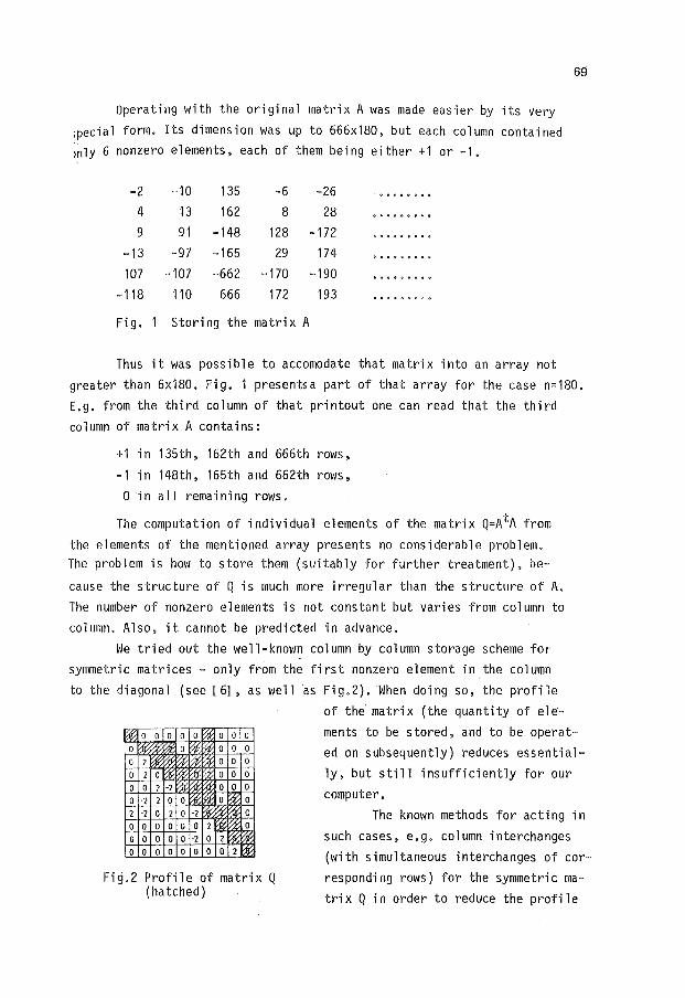
Operating with the original matrix A was made easier by its very ;pecial form. Its dimension was up to 666x180, but each column contained )nlY 6 nonzero elements, each of them being either +1 or -1.
-2 -10 135 -6 -26 . 0 • ~ 0 " • 0 0
4 13 162 8 28 0." ....... 0
9 91 -148 128 -172 o o oe• "" o o
-13 -97 -165 29 174 .... 0" 0 0 0"
107 -107 -662 -170 -190 • 000" ..... 0
-118 110 666 172 193 ........... 0 ..
Fig. Storing the matrix A
69
Thus it was possible to accomodate that matrix into an array not greater than 6x180. Fig. 1 presentsa part of that array for the case n=180. E.g. from the third column of that printout one can read that the third column of matrix A contains:
+1 in 135th, 162th and 666th rows,
-1 in 148th, 165th and 662th rows. 0 in all remaining rows.
The computation of individual elements of the matrix Q=AtA from the elements of the mentioned array presents no considerable problem. The problem is how to store them (suitably for further treatment), be-
cause the structure of Q is much more irregular than the structure of A. The number of nonzero elements is not constant but varies from column to column. Also, it cannot be predicted in advance.
~Je tried out the we 11-known co 1 umn by co 1 umn storage scheme for symmetric matrices - only from the first nonzero element in the column to the diagonal (see [ 6], as well ·as Fig.2). When doing so, the profile
Fig.2 Profile of matrix Q (hatched)
of the· matrix (the quantity of elements to be stored, and to be operated on subsequently) reduces essentially, but still insufficiently for our computer.
The known methods for acting in such cases, e.g. column interchanges (with simultaneous interchanges of corresponding rows) for the symmetric rna-trix Q in order to reduce the profile
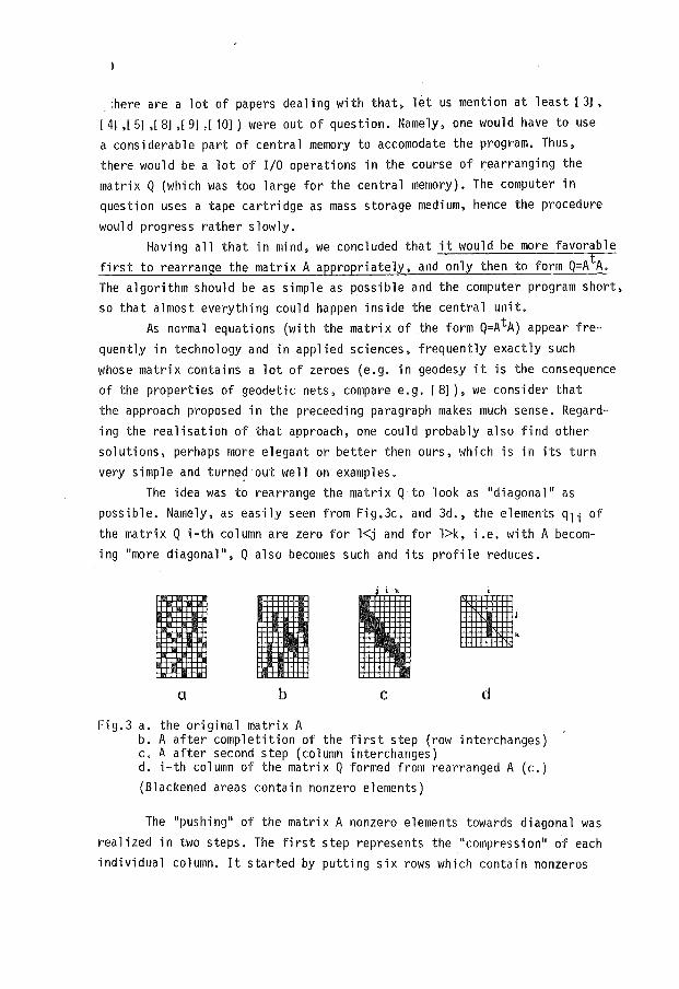
;here are a lot of papers dealing with that, let us mention at least [ 3], [~ ,[~ ,[8] ,[9] ,[ 10]) were out of question. Namely, one would have to use a considerable part of central memory to accomodate the program. Thus, there would be a lot of I/0 operations in the course of rearranging the matrix Q (which was too large for the central memory). The computer in question uses a tape cartridge as mass storage medium, hence the procedure would progress rather slowly.
Having all that in mind, we concluded that it would be more favorable first to rearrange the matrix A appropriately, and only then to form Q=AtA. The algorithm should be as simple as possible and the computer program short, so that almost everything could happen inside the central unit.
As normal equations (with the matrix of the form Q=AtA) appear frequently in technology and in applied sciences, frequently exactly such whose matrix contains a lot of zeroes (e.g. in geodesy it is the consequence of the properties of geodetic nets, compare e.g. [ 8] ) , we consider that the approach proposed in the preceeding paragraph makes much sense. Regarding the realisation of that approach, one could probably also find other solutions, perhaps more elegant or better then ours, which is in its turn very simple and turne? out well on examples.
The idea was to rearrange the matrix Q to look as "diagonal" as possible. Namely, as easily seen from Fig.3c. and 3d., the elements qli of the matrix Q i-th column are zero for l<j and for l>k, i.e. with A becoming "more di agona 1", Q a 1 so becomes such and its profi 1 e reduces.
i
II: a b c d
Fig.3 a. the original matrix A b. A after completition of the first step (row interchanges) c. A after second step (column interchanges) d. i-th column of the matrix Q formed from rearranged A (c..)
(Blackened areas contain nonzero elements)
The "pushing" of the matrix A nonzero elements towards diagonal was realized in two steps. The first step represents the "compression" of each individual column. It started by putting six rows which contain nonzeros
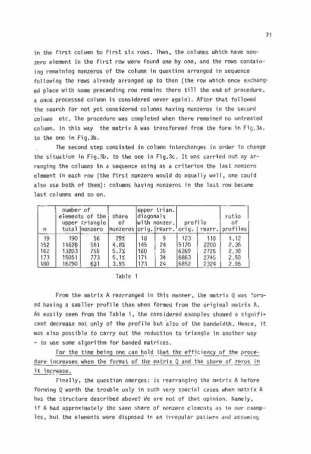
71
in the first column to first six rows. Then, the columns which have nonzero element in the first row were found one by one, and the rows contain
ing remaining nonzeros of the column in question arranged in sequence following the rows already arranged up to then (the row which once exchanged place with some preceeding row remains there till the end of procedure, a once.processed column is considered never again). After that followed
the search for not yet considered columns having nonzeros in the second column etc. The procedure was completed when there remained no untreated column. In this way the matrix A was transformed from the form in Fig.3a.
to the one in Fig.3b. The second step consisted in column interchanges in order to change
the situation in Fig.3b. to the one in Fig.3c. It was carried out by arranging the columns in a seguence using as a criterion the last nonzero element in each row (the first nonzero would do equally well, one could also use both of them): columns having nonzeros in the last row became
last columns and so on.
number of upper trian. e 1 ements of the share diagonals ratio
upper triangle of with nonzer. profile of n total nonzero non zeros orig. rearr. ori g. rearr. profiles
19 190 56 29% 18 9 123 110 1.12 152 1162~ 561 4.8% 145 24 5170 2200 2.35 162 13203 755 5.7% 160 35 6269 2725 2.30 173 15051 773 5.1% 171 34 6863 2745 2.50 180 16290 6~1 3.9% 173 24 6852 2324 2.95
Table 1
From the matrix A rearranged in this manner, the matrix Q was formed having a smaller profile than when formed from the original matrix A. As easily seen from the Table 1, ·the considered examples showed a signifi
cant decrease not only of the profile but ~lso of the bandwidth. Hence, it was also possible to carry out the reduction to triangle in another way - to use some algorithm for banded matrices.
For the time being one can hold that the efficiency of the procedure increases when the format of the matrix Q and the share of zeros in it increase.
Finally, the question emerges: Is rearranging the mr>tri x A before forming Q worth the trouble only in such very special cases when matrix A has the structure described above? We are not of that opinion. Namely, if A had approximately the .same share of nonzero elements as in our examples, but the elements were disposed in an irregular pattern and assuming
.. _.e heterogenous values, A would fit into an array of something more
than b1ofold magnitude, which would be still bearable. In that case e.g. for n=180, in place of an 6x180-array, one would need approximately 13x180 of storage space. Table 1 shows that it would be still less even than the profile of the matrix Q formed from the rearranged A.
REFERENCES
1. BJERHAMMAR A.: Theory of errors and generalized matrix inverses, Elsevier Scientific Publishing Company, Amsterdam 1973
2. CIGROVSKI B.: Accuracy analysis of the observations for the part of the second order trianqulation net in the boundary region of SR Croatia and SR BandH (Croatoserbian), master's thesis (in preparation for publication)
3. DUFF I. S., REID J. K.: A compmoison of sparsity orderings for obtaining a pivotal sequence in Gaussian Elimination, J. Inst. Maths Applies 14(1974), 281-291
4. FUCHS G. von, ROY J.R., SCHREM E.: Hypermatrix solution of large sets of syrrrmetrlc pos?:Uve-definite linear• equations, Computer Methods in Applied Mechanics and Engineering 1(1972), 197-216
5. GIBBS N.E., POOLE W.G.Jr., STOCKMEYER P.K.: An algorithm for reducing the bandwidth and pr•ofi le of a sparse matrix, SIAM J. Numer. Ana 1 . 2(1976), 236-250
6. JENNINGS A.: A compact stor·age scheme for the solution of symmetric linear simu Ztaneous equations, The Computer Journa 1 9 ( 1966), 281-285
7. MIHAILOVIc K.: Geodezija II (I part), (Serbocroatian), Gradjevinska knjiga, Beograd 1974
8, STEIDLER F,: Zur Lusung gPossmo schwach besetzter Normalgleichungssysteme in der geodatischen Netzausgleichung, Zeitschrift fUr· Vermessungswesen 3(1982), 97-108
9. TEWARSON R.P.: Sparse matrices> Academic Press, New York and London 1973
10. WAI-HUNG LIU, SHERMAN A.H.: Comparative analysis of the CuthiU-McKee and the revel'se CuthiU-McKee order1:ng algorithms for aparose matrices, SIAM J. Numer Anal. 2(1976), 198-213.
11. WOLF H. : Ausg·[eichungsrechnung II, Ferd. DUmml ers Verlag, Bonn 1979

.. ~ .. 1erical Methods and
Approximation Theory
Nis, September 26-28, 1984
APPROXIMATION OF 2n - PERIODIC FUNCTIONS BY FUCTIONS OF SHORTER PERIOD
Slobodan D, Miloradovic
ABSTRACT:
In this paper we give the value of the exact approximation, for a fix~d. 2n ~ periodic function by functions of period 2n/k vJhere k is a natural number larger than 1. We determine also the exact approximation of a fixed 2n ~ periodic fuction by fwiktions of period 2nm/k, where m al?-d, k are two nutuaZZy prime integers, Them the equality of both approximations is pro~ed. An example which illustrates these results is given at the end.
1PROKSIMACIJE 2n - PERIODICNIH FUNKCIJA FUNKCIJAMA KRAGE PERIODE. U r>adu 3e daje vrednost taone aproksimaaije, fiksirane, 2n - periodiGne funkaije runkaijama perioda 2n/k gde je k prirodan broj vedi od 1. Takodje se utvrijuje tacna aproksimac~ja, fiksirane, 2n - periodio7(e funkaije fun7wijama perioda .2nm/k, gde su m i k prirodni, uzajamno prosti, brojevi. Zatim se dokazuje jednakost jedne i druge aproksimacije. Na Jo:.aju se daje primer koji lustruje naV@dene rezultate.
~et cra,b], as usaul be the space of real continuous functions f defined on the ·interval [a, b] with norm
II fllqa,bJ = x 6[:~b] lf{x) I,
and let C denote the space of periodic, real and continuous functions f defined on the real line (-oo, +oo), whose period is 2n multiplied by a rational number, with norm
llfllc = maxlf(x) I, X
The set of all periods of a functions f is denoted by ~f· For example, iff is a 2n - periodic functlon, we shall write 2n6~f'
In this paper weshall find the value of the exact approximation of a fixed 2n - period ica 1 function f, by a functions 1/J of period 2nm/ k, v:here m and k are two mutually prime integers, that is, we shall find the value of
73
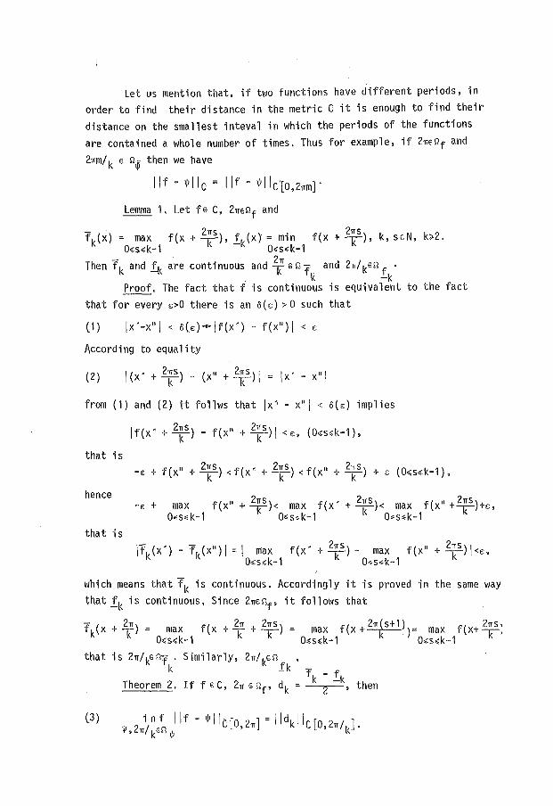
Let us mention that, if two functions have different periods, in
order to find their distance in the metric C it is enough to find their
distance on the smallest inteval in which the periods of the functions
are contained a whole number of times, Thus for example, if 2nenf and
2nm/k € n~ then we have
!If~ 1/JIIc = !If- 1/JIIc'[o,2nm]"
Lemma 1. Let fG C, 2nenf and
fk(x) = max f(x + 2~s), fk(x)· =min f(x + 2~s), k, seN, k<>2. O.;;s..;k-1 O<s<k-1
- 2n Then f k and fk are continuous and Ten f 1< and 2n/ k€Q fk
Proof. The fact that f is continuous is equivalent to the fact
that for every c>O there is an 6{e:) > 0 such that
(1) !x'-x"l < 6(c)=\f(x')- f(x")! < e:
According to equality
(2) \(x' + 2ks)- (x" + 2~5 )! = !x'- x"l
from (1) and (2) it fo1lws that !x''- x"l < 6(e:) implies
\f(x' + 2ks) - f(x" + 2~5 ) I< e:, (O<>s<k-1),
that is -e: + f(x" + 2~s) < f(x' + 2ks) < f(x" + 2~s) + c (0.-s<k-1),
hence -c + max f(x" + ~)< max f(x' + 2ks)< max f(x" + 2ks)+c,
Q.;s.;k-1 0" s" k-1 O.;s,k-1
that is jfk(x') - fk(x") I= I max f(x' + 2ks)- max f(x" + 2ks) l<c,
O<s.:k-1 O"s"k-1
which means that fk is continuous. Accordingly it is proved in the same way
that fk is continuous, Since 2n£nf' it follows that
fk(x + 2;) = max f(x + 2; + Jks) = max f(x + 2n~s+ 1 ))= max f(x+ 2k5]
O<s<k-1 o,s..;k-1 O<s<k-1
that is 2n/kenr. Similarly, 2n/ken k fk T _ f
Theorem 2, Iff € C, 2n ,;nf' dk = k 2 -k, then
(3) i n f II f - 1/J II c [o 2 -J = i I d k II c [o 2 I J 1/J 2n/ €Q ' TI ' TI k •
' k 1/J
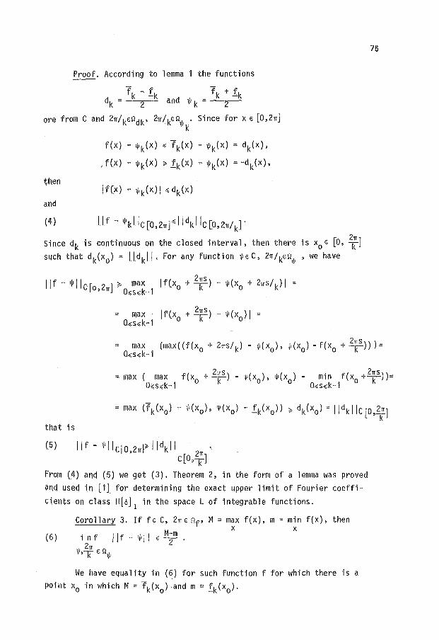
Proof. According to lemma 1 the functions
fk~·fk fk+.fk dk = 2 and lJ! k = 2
ore from C and 2TI/kEr.ldk' 2u/kEr.llJ!k' Since for x € [0,2TI]
then
and
f(x) - lJ!k(x) ~ fk(x) - lJ!k(x) = dk(x),
, f(x) "'lJ!k(x) ".fk(x) - lJ!k(x) = -dk(x),
(4) !.If- lJ!kllq0 , 2 'ITr~lldkllc[o,2'IT/k]'
Since dk is continuous on the closed interval, then there is x0 € [0, 2;J
such that dk(x 0 ) = jjdkjj, For any function ;JiEC, 2TI/k€r.llJ!, we have
that is
(5) ilf-lJ!ilcjo, 2 'ITI~IIdkll 2'IT
c[o,T]
From (4) and (5) we get (3). Theorem 2, in the form of a lemma was proved
and used in [1J. for determining the exact upper limit of Fourier coeffi
cients on class H[8] 1
in the space L of integrable functions.
(6)
Corollary 3. If fE C, 2TI€ rolf' M =max f(x), m =min f(x), then M X X
inf jjf-;JJjj.; ;m. 2'IT
lJ!,T€r.!lJ!
We have equality in (6) for such function f for which there is a
point x0 in which M = fk(x0
) .and m = .fk(x0
).
75
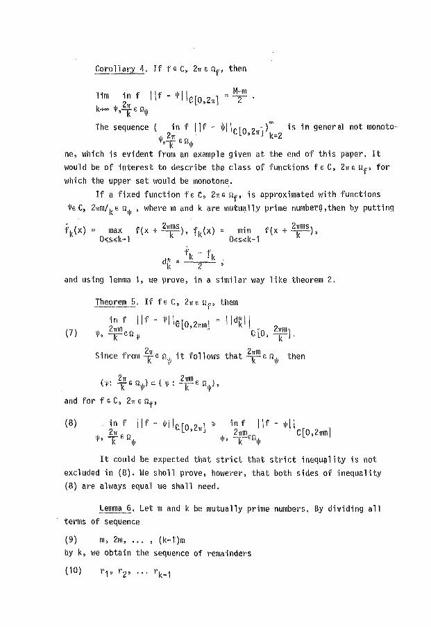
Corollar·y 4, If f E C, 2TI e rip then
lim ~~ f \If- lj!llqo,z1T] = M2m • k-j><)O ljJ,kErlljJ
The sequence ( in f \If- ~llc[o 2 ])"" is in general not monoto-2TI ' 1T k=2
ljJ,Ter~ljJ
ne, which is evident from an example given at the end of this paper. It
would be of interest to describe the class of functions fE C, 2TIE r~f' for
which the upper set would be monotone.
If a fixed function f£ e, 21re rip is approximated with functions
2Tim/kE r~ljJ, where m and k are mutually prime number~,then by putting
max f(x + Z1rms), fk(x) = min f(x + Z1rms), O<!ls.;;k-1 k O~s~k-1 k
fk - fk dk = 2
and using lemma 1, we prove, in a similar way like theorem 2.
Theorem 5. If fE C, 2TIE r~f' them
(7) ~~mf \If- lj!llqo,21Tm] = \\dkl\ [ 21Tm1
lj!, T6rlljJ e: o, -k- .
Since from 2k6r11/J it follows that 2kmer~ljJ then
2TI 21rm H: Ter~1/J}c:{1/J: -1<-E.r~ljJ},
and for f s C, 2TI e rip
2;n1T f \If- lj!llqo,z1T] ~ in f \If- ljJII
2TimE.rl · C[0,2Tim] ljJ'k 6 rlljJ ljJ, k lj!
(8)
It could be expected that strict that strict inequality is not
excluded in (8). We sholl prove, howerer, that both sides of inequality
(8} are always equal we shall need.
Lemma 6, Let m and k be mutually prime numbers. By dividing all terms of sequence
(9} m, 2m, .•. , (k-t)m
by k, we obtain the sequence of remainders
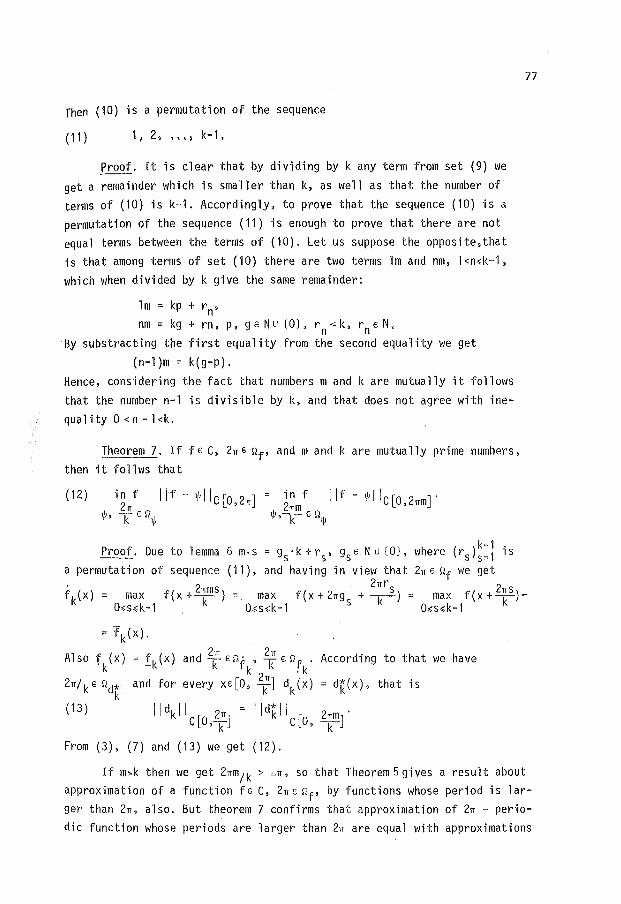
rhen (10) is a permutation of the sequence
(11) 1, 2, '"' k-1,
Proof. It is clear that by dividing by k any term from set (9) we get a remainder which is smaller than k, as well as that the number of terms of (10) is k-1. Accordingly, to prove that the sequence (10) is a permutation of the sequence (11) is enough to prove that there are not equal terms between the terms of (10}. Let us suppose the opposite,that is that among terms of set (10) there are two terms lm and nm, l<n~k-1,
which when divided by k give the same remainder:
1m= kp + rn' nm =kg+ rn, p, geNu {0}, rn<k, rne N,
By substracting the first equality from the second equality we get (n-l)m = k(g-p).
Hence, considering the fact that numbers m and k are mutually it follows that the number n-1 is divisible by k, and that does not agree with inequality 0 <n -l<k.
Theorem 7. Iff£ C, 2rrE stf' and m and k are mutually prime numbers, then it follws that
Proof. Due to lemma 6 m.s a permutation of sequence (11),
in f II f - 1J! II C [o' 2rrm] . 2rrm
1}!,-k- 6 S"ll}J
( ) k-1 . = gs·k+r5
, gse Nu{O}, where rs s= 1 1s and having in view that 2rr E stf we get
77
fk(x) max f(x + 2'kms) = O,:s,:k-1
2rrr s 2 s max f(x + 2rrgs + ~) = max f(x ++)=
O~s~k-1 O,:s~k-1
=fk(x}.
Also f (x) =.fk(x) and 2;6&1-f, 2;£stf. According to that vie have k k . k
2rr/k6 std* and for every xe[O, 2;] dk(x) = dk(x), that is k
( 13) II dk II [ 2rr, II d"k II [ 2rrmJ · C O,kj C 0, k-
From (3), (7) and (13) we get (12}.
If m>k then we get 2rrm 1 k > L rr, so that Theorem 5 gives a result about approximation of a function fE C, 2rr6 stf' by functions whose period is larger than 2rr, also. But theorem 7 confirms that approximation of 2rr periodic function whose periods are larger than 2rr are equal with approximations
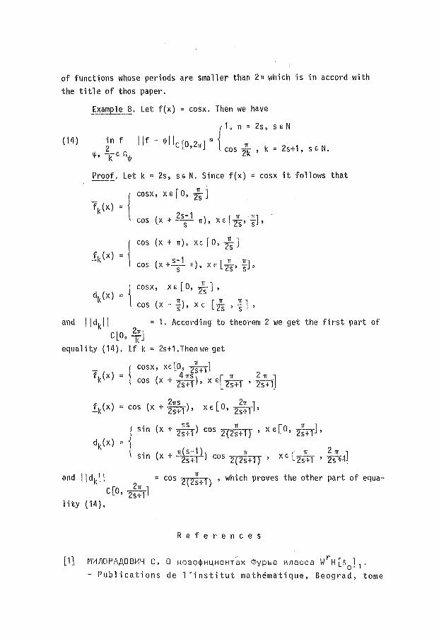
of functions whose periods are smaller than 2n which is in accord with the title of thos paper.
( 14)
Example 8, Let f(x) = cosx. Then we have
{
1, n = 2s, s € N
II t - 1/J II r. J = CL0, 2n cos;k,k=2s+1,seN.
Proof. Let k = 2s, S€ N. Since f(x) = cosx it follows that
COSX, X€ [0, Ts J
(X + 2s-1 ) [ 1r · n] cos 5 n , X 6 -zs• s '
= ( cos (X + n ) , X £ [ 0 , 2n5 ]
i ( s-1 ) [ n n] COS X +-5- n , X E 7$' S '
_ \ cosx, x £ [ 0, !s ] , dk (x)
cos (x- ~),X£ [-fs, ~],
and I ldkl I = 1. According to theorem 2 we get the first part of C[O, ~]
equality (14), If k = 2s+1.Thenwe get
{ cosx, X£ [0, Z;+,J
f (x) = hs [ n 2 n J k cos (x + 2s+1)' x 6 2s+1 ' 2s+1
( 2ns ) [ 2n ] fk(x) = cos x + 2s+1 ' x € 0, 2s+1 '
. ( ns ) n = J Sln x + 2s+1 cos 2(2s+1) ,
l · ( ~) n Sln x + 2s+1 cos 2{2s+1)
X € [0, 2;+1)'
and I ldkl \ =cos 2(2;+1) , which proves the other part of equa-C[O, 2~: 1 ]
1 i ty ( 14).
R e f e r e n c e s
[1] / r MHnDPAAOBHY C, 0 Hos¢¢H~HBHTax ¢ypbe Hnacca W H[o0
] 1 .
-Publications de 1 'institut mathematique, Beograd, tome
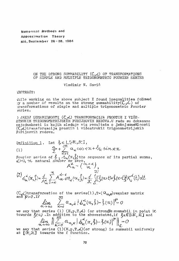
Numerical Methods and
Approximation Theory
Nis, September 26-28, 1984
ON THE STRONG SUMMABILITY (C,~) OF TRANSFORMATIONS OF SIMPLE AND MULTIPLE TRIGONOMETRIC FOURIER SERIES
Vladimir N. Savio
'I.BSTRACT:
Vhile working on the above subject I found inequalities followed w a number of result's on the strong summability(C,rf~) of ;ransformations of simple and multiple trigonometric Fourier Jeries.
) JAKOJ SUMABILNOSTI (Cj~) TRANSFORMACIJA PROSTIH I VISESTRUKIH TRIGONOMETRIJSKIH FURIJEOVIH REDOVA.U radu su dokazane nejednakosti iz kojih sleduje niz rezultata o jakojsumarnlnosti CC,~)transformacija prostih i visestrukih trigonometrijskih Furijeovih redova.
CC~£)transformation of the series(l),T=(O~~regular matrix and tJ>O. If oo
1vm I a/~~.,; I ~~e-x_,,~)- ~c~~) I~"' o "'t --+ 00 K'"' ()
we say that series (1) (H,p,T,o(,) (or strong1is summabil in point X towards ~('..C) .In ad2tion to the abovestated,i~ ~£<i'.&:Jr? X] and
l;;m. /} L ctn, i< J Co d..(~,~)- }(/x) 1· y.> \\ = 0 1'L-'>-00 K=O ~ I<: I c
we say that series (l)(H,p,T,~)(or strong) is summabil uniformly at [-:Jt7X] towards the f function.
79

Theorem ~~Let !~il:(-:~·1Jc.]th:Jn for each r~ .. ~,~~-'1 1 ~.._~C ~.Jl-6~( JC, ~)~ !(·)t,;! rJ ~~-eli cy..,·v~,[ K_hL;~ c~D r i .. ~.
where J..,-.J is any non-negative ,not-increasing numbers ,E~( ~ 1 the best approximation of the f function to the trigonometric polYJ:!omials of the degree ~\J'in distanceof the space If .[~It ~ii..], and cl\ (f',J.) a positive constant aepending only on r a.nli,.;,'
Proof.According to Theorem l there follows
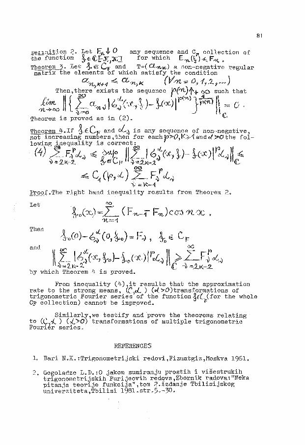
JJenni:tiPJ]-_Z. Let F..,~ J, 0 any seqUf;mce and CF. collection of the functJ..on !e<tE-Jr,:X:] for wh1ch E-n.(~J~F.-vc." Theorem 3· Let ~ E CF and T=( CL,~,~) a non-negative regular -matrix the elements of which satisfy the condition
an/<+1 ~ a_n;sK (V~ = 0:1 1~.:2. 7 .... ) Then, there exists the sequence jO(rtt.)t+ 00 such that
J.;-, Jl { f' \ "-· Q ) Q .I rc-n.) l~ 1\ -n~~ . ~ ~ a-n.J ~~ ('.t.,-;~ - .r(r:x:,) ) ~"'"·' ~~ = o . Theorem is proved as in (2). C
Theorem 4.If !,E.CF and cL~ is any sequence of non-negative, not increasing num·bers, then for each p>O, V:~·1 and o(>O the following inequality is correct:
(.q) ~- F.t~-1) ~ ;x'-~ }jZJ 6:(;~:,-l)- ~c~){r,x:-v!{ ~ :V:2.K:-2. ~eCF ~=.2.K-..2. C
. . oo r .~ C1 cr,oG) 7= F~ ~~
II :. ¥::-1 Pro~f.The right hand inequality results from Theorem 2.
co
~o (-:x:) -L ( Fn.-1 F -n.) c OJ n x . ")t.=.1
Let
Then ~.o(0)-6:(o,~o)= F~, ~0 t Ls:
DC
)\ L \6~('Jt,-~o)-·~0 ('~.)~fq£~ !\ >LF% a(.~ ~::2..1:.~ '2. ( +=-.J..K-2.
by which Theorem 4 is proved. -
and
81
From inequality (4),it results that the approximation rate to the strong means, ((\tL ) (c( >0 )transformations of trigonometric Fourier series of the function!((.(for the whole CF collection) cannot be impr,oved. I=
Similarl~,we testify and prove the theorems relating to ((,.{, ) (,/,_">0) transformations of multiple trigonometric Fourier series.
REFERENCES
l, Bari N.K.:Trigonometrijski redovi,Fizmatgiz,Moskva 1961.
~. Gogoladze L.D.:O jakom sumiranju prostih i visestrukih trigonometrijskih Furijeovih redova,Zbornik radova:"Neka pitanja teorije funkcija",tom 2.izdanje Tbilisijskog univerziteta,Tbilisi 198l.str.5.-30.

I
I
I
I
I
I
I
I

Numerical Methods and
Approximation Theory
Nis, September Z6-28, 1984
~ ESTIMATION FOR REMAINDER OF ANALYTICAL FUNCTION IN TAYLOR'S SERIES
•etar M. Vasic, Igor z. Milovanovic and Josip E. Pecaric
.BSTRACT: n this paper some estimations of difference modul of analyical functions 'l.nd referred Taylor's polynomials are given. he obtained results are illustrated on a certain concrete f cases, i.e. on exponential, sinhyperbolic and cosinhyperolic function.
OCENI OSTATKA ANALITICKE FUNKCIJE U TAYLOROVOM RAZVOJU. U ovom radu date su neke ocene modula razlika analitickih funkcija i odgovarajucih Taylorovih polinoma. Dobijene ocene su ilustrovane na konkretnim slucajevima, tj. na eksponencijalnoj, sinushiperbolicnoj i cosinushiperbolicnoj funkciji.
We shall prove first a more general result for analytical functions:
THEOREM l. Let z~+ f(z) be an analytical function in the circle izl< R. Let functions z~+ f(k)(z), ke=N0 ~ map real axis in real axis. If a natural number r exist, l < r ~ n, so that 0~ f(n+k)(O) ~ ir+k)(O) - -
- - , ke. N, the inequality
holds. Proof. Assume that all conditions given in theorem 1
are fullfiled. ·Then
it(z)- ~ f(k\o2 zkl'" I ~oo f(k)(O) :4kl~ ~oof(k\?lizlk k=O kl k=n+l kl k=n+l
83
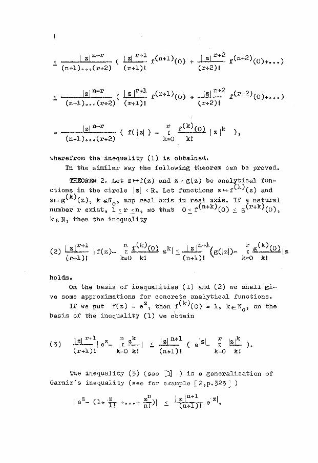
<
<
lzln-r __ ~...;;;. "-· -- ( f( lzl)-
(n+l) ... (r+2) ),
wherefrom the inequality (l) is obtained.
In the similar way the following theorem can be proved.
THEOREM 2. Let z t-+f(z) and z..,. g(z) be analytical fun
ctions in the circle lzl < R. Let functions z H-f(k)(z) and
ZH- g(k\z), k eN , map real axis in real axis. If a natural number r exist, ~ _:_ r _:_ n, so that 0 _:_ f(n+k) (0) ,;;, g(r+k) (0),
k E. N, then the inequality
I z lr+l n f(k)(O) k 1 ~ 1n+l( r (k)(O) (2) · · I f(z)- ~ z I_:_~ g(lzl)- ~ g lz
(r+l) I k=O kl (n+l) 1 k=O kl
holds.
On the basis of inequalities (1) and (2) we shall gi
ve some approximations for concrete analytical functions.
If we put f(z) = ez, then f(k)(O) = 1, kEN0
, on the
basis of the inequality (l) we obtain
(3) 1 .. 1 r+l z ~le(r+l)!
n k ~ _z_l <
k=O k!
lzl n+l I I ( e z-(n+l)!
~ lzlk /., ) .
k=O k!
The inequality (3) (see [~ ) is a generalization of
Garnir's inequality (see for example [ 2,p.323 J )
z z zn I z ln+l I zl I e- (1+ 'rr + ... + n!)l < (n+l)! e •

and
If we put that
7.: 2n-l z..... z T2n-l(z) = z + ?T + ••• + ~(~2n--~r~)~!
2n-2 z • • • + ~( ~2n--""'2"') I '
then for .f(z) shz and .f(z) = ch z we obtain inequali-
ties
and
f ( )I (2n-2m~ 1 ch z - T2n_2 z 2_ (2ri I
for m=l, ••• ,n, respectively.
In the same way on the basis of tne inequality (2)
we obtain inequalities
I , < \1 (2n-2m~t 1 _,2m+lc II . <I'') sh z - 1'2n-l z Jl ~ (2ri+l ! L.J ch z- ·r2n-2m-2 zv
and
rch z- T2
n_2(z)l < ( 2n-2m+l·)!lz.2m-l(shlzi-T (I z/)) (2n)! 1- 2n-2m-l
form= O,l, ••• ,n • On the basis of P.R.Beesack's remark (see l2] ) we
shall prove the .following result:
85
THIDREM 3. If z is the complex number, iz I~/ ( 2n+2) ( 2n+ 3}
then the inequality
< (2n+2)(2n+3) ___ __:.l;;;;.z:...f 2_n_+_1__,,..
(2n+l)! (2n+2)(2n+3)-l zl 2
holds.
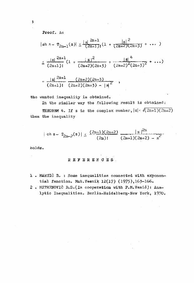
Proof. As
I zl 2n+l lzl 2 Ish z- T2n-l (z)l ~ (2n+l)l (l + (2n+2)(2n+3) + • • • )
< lzl 2n+l I z1 2 lzl 4 . . (l + . . + 2 2 + ••• )
(2n+l) I (2n+2)(2n+3) (2n+2) (2n+3)
I zl 2n+l __ (;h2;;;::n:.:+..:;;2~)~( ;::;;2n:::.+;..,3~).__...,.. . . 2
(2n+l) I (2n+2)(2n+3) - I z1
the wanted inequality is obtained~ In the similar way the .follo1t!ing result is obtained:
THIDREM 4. If z is the complex number, lzl< /(2n+l)(2n+2) then the inequality
holds.
REFERENCES
1 • MARTie B. : Some inequalities connected with exponential function. Mat.Vesnik 12(17) (1975),163-166.
2 a MITRINOVIC D.S.(In cooperation with P.M.Vasi6): Analytic Inequalities. Berlin-Heidelberg-New York, 1970.
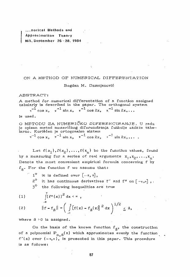
.. -.nerical Methods and
Approximation Theory
Nis, September 26-28, 1984
ON A ME'.THOD OF NUME'.RICAL DIFFERE'.NTATION
Bogdan M. Damnjanovi6
ABSTRACT:
A method for numerical differentation of a function assigned tabelarly is described in the paper. The orthogonal system
-1 -1 . -1 -1 . 11 cos x, 11 s1n x, 11 cos 2x, 11. s1n 2x, .••
is used.
0 ME'.TODU ZA NUMERICKO DIFERENCIRANJE' .• U radu je opisan metod numerickog diferenciranja fuhkcije zadate tabelarno. Koris6en je ortogonalan sistem
-1 -1 . -1 -1 11 cosx, 11 smx, 11 cos2x, 11 sin2x, ••.
Let f(x1 },f(x2 }, ... ,f(xn} be the function values, found
by a measuring for a series of real arguments x 1 , x2 , ••• , xn.
Denote the most convenient empirical formula concerning f by
f 13
• For the function f we assume that:
( 1}
( 2}
it is defined over [-11,1TJ,
it has continuous derivatives f' and f" on [ -11,11] ,
the following inequalities are true
1T 2 J (f" ( x} } dx < co ,
-1! ( 1T 2 ) l/2 llf-f13 11= _l[f(x}-f13 (x}] dx <B,
where .13 > 0 is assigned.
On the basis of the known function f 8 , the construction
of a polynomial P ,(x} which approximates evenly the function n,~ ~
f' ( x} over (- 11, 11} , is presented in this paper. This procedure
is as follows:
87

The known function f B is approximated by a polynomial
q (x) of degree n+l, such one that the inequality ,n+l
( 3) II f B - qn+l II ~ B
holds, The polynomial qn+1 is obtained developing f B by Fourier'
series using the orthogonal system
-1 -1 . -1 2 -1 . 2 11 cos x, 11 stn x, 11 cos x, 11 stn x , ••• ,
namely,
( 4)
where
(5)
qn+1(x)
11
ak = J fB( x) cos kx dx, -11
11
bk = j f 13 (x) sinkxdx, -11
and n is chosen so that ( 3 ) is valid.
According to ( 2) and ( 3) it follows
(6) llf-qn+111 ~ llf-fBII+ llfB-qn+1ii,;;, 2 B·
If the function f' is marked by f'(x) = u (x), then under 0
the condition ( 1) u ( x) is the unique solution of the integral 0
equation X
(7) ju(t)dt=f(x). -11
Let (7) be written in the operator form
(8) Au = f.
Introducing the functionalls
and
( 10) K [u] = II u'll2 ,
the approximate solution of the equation ( 7) (i.e. ( 8) ) can be
found by minimizing the functional K [ u J under the condition
( 11) I [u, qn+1] :<. 4B2
(according to (6}). Denote a such minimum by uB( x}. Then, it
is easy to prove that
(12}
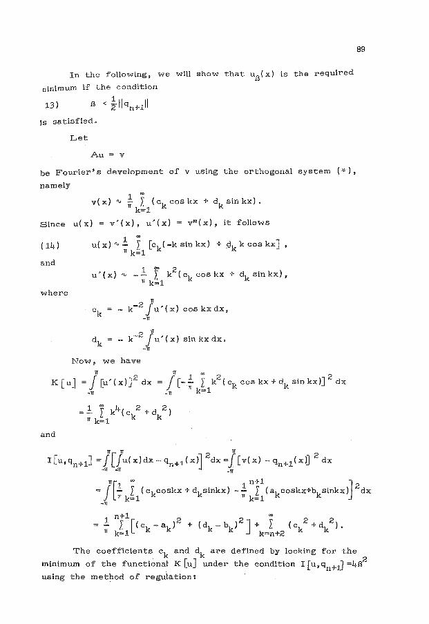
In the following, we will show that uB( x) is the required
ninimum if the condition
13) B < ~~~qn+111 is satisfied.
Let
Au= v
be Fourier's development of v using the orthogonal system ( ¥ ) ,
namely
Since
(14)
and
where
and
1 00
v(x) "' - I (ck cos kx + dk sin kx). 1T k=1
u(x) = v'(x), u'(x) = v"(x), it follows
1 00
u( x) "'- I [ck( -k sin kx) + _gk k cos kx] , 1T k=1
1 ()0 2 u' ( x) "' -- I k ( ck cos kx + dk sin kx) ,
1T k=1
1T
ck k-2 j u'(x) cos kxdx, -1!
dk = - k - 2 j u' ( x) sin kx dx. -1T
Now, we have
89
rr[1 oo 1 n+1 J 2 = J - I ( ckcoskx + dksinkx) -- I ( akcoskx+bksinkx) dx
1T k=1 1T k=1 -1!
The coefficients ck and dk are defined by looking for the
minimum of the functional K [u] under the condition I [u, qn+1] =4B2
using the method of regulation:

.P[u,qn+1] = K [u] + n I [u, qn+1] , I [ u, qn+1] 4B2
.
If we put A=~ > 0, then .P[u,qn+1J becomes
1 n+1 2 2 .P[u,qn+1] = ;-kL [ (ck-ak) +(dk-bk) J
+ f ( ck 2 + bk 2) + 2. I k4 ( ck2 + bk 2) k=n+2 TI k=1
1 n+\ 2 2 2 A 4 2 2 J ; kLL( ck - ak ) + ( dk - bk) +if k ( ck + bk )
+ I (:} + ~k4)( ck2 + dk2). k=n+2
Since the second sum is nonnegative, for the minimum is supposec
that ck-+ 0 and dk -+0 for k;;;,n+2. Then, according to
and
we find
(15)
(lljl = 0 I
3dk
On the basis of ( 14) we obtain
( 16) 1 n+1 ak cos kx + bk sin kx UB ( X) = iT I 4 '
k=1 1 + A k
where A is determined from
( 1 7) II uB- qn+1ll2
= 4B2
•
that is
(18)
The left-hand side of ( 18) is monotonically increasing fun
ction of A which tends to
n+1 .l I(a2+b2) 'IT k=1 k k
when A -+ "'• Besides, B -+ 0 if A -+ 0 so that
(19) 1 n+1 2 2 2 iT I ( ak + bk ) > 4B ,
k=1

, .. --_from we immediately ( 13). Therefore, u 8 ( x) will be mi
imum of <P[u,qn+-1] if (13) is valid.
It is easy to prove that u13
(x) is minimum of 1l [u,qn+1]
tor each x E(-rr,rr) and lim u13
(x) = u (x) = f'(x) evenly on B -'>-0 °
( -rr, 1T) •
According to the above, the polynomial P 0 ( x) has the n ',,
form
1 n+1 ak cos kx + bk sin kx P B(x) =- L 4 '
n, rrk=1 1+Ak
AT here ak, bk and A are defined by ( 5) and ( 18) •
REFERENCES
BAHVALOV N.: Numerical methods. Nauka, Moskva 1973.
~. DOLGOPO~LOVA T., IVANOV V. : 0 cislennom differencirovanii. 2. vices!. matem. i matem. fiz. 3 ( 1966), 570-576,
3. MOR 020V A. : 0 zadace diferencirovania i nektorih algoritmah priblizenia eksperimentalnoj informacii. Vi cis!. metodii i programirovanie, MG U 1970, 46-62.
91

I
I
I
I
I
I
NUIIHHical Methods and
Approximation Theory
Nis, September 26-28, 1984
ON AN APPLICATION OF HERMITE'S INTERPOLATION POL YNOIVIIAL AND SOME RELATED RESULTS
GRADIMIR V. MILOVANOVIC AND JOSIP E. PECARIC
ABSTRACT: In this paper we gave generalizations and improvements of integral ine
qualities from ClJ and C2J. In the proof we used the weU-known re
sult for the error of Hermite's interpolation polynomial. Some similar
results are aZso given.
0 JEDNOJ PRIMENI HERMITEOVOG INTERPOLACIONOG POLINOMA I NEKIM SRODNIM REZULTATIMA, U radu su date generaZizaaije i poboljSanja in
tegraZnih nejednakosti iz ClJ i C2J. U dokazu je korisden poznati rez
uZtat za gresku Hermiteovog interpolaaionog poZinoma. Neki sZiani rezul
tati su takodje dati.
1. INTRODUCTION
In the journal Amer. Math. Monthly the following two
problems ([1],[2]) are posed:
1° Suppose f(x) has a continuous (2m)-th derivative
on a~ x ~ b, that lfC 2m\xJ I ~ M, and that f(r) (a) "' f(r) (b)
~ 0 for r=O,l, ••• ,m-1. Show that
b
(1) )f(x)dx ~ a
(m! )2
tvJ .- -(b-a/m+l. (2m)! (2m+l)!
2° Let f: [a, b] -+R be a. continuous function which is
twice differentiable in (a, b) and satisfies f(a) = f(b) = u.
Prove that b
(2) )lf(xJidx ~ JL M(b-a)3, a 12
\'There M= suplf"(xJI for xE(a,b).
93
The solution of first problem is given in [3].
The inequalities (1) and (2) are related to IYENGAR's
inequality [4, PP• 297-298] l).
In this paper \>Je shall prove some inequalities which
generalize (1) and (2) in many senses.
Let us define the two-parameter clas of polynomials
P~m,k) (0 ~ m ~ k < n; m,k,n f:N) by means of
p(m,k)(x) E p(m,k)(x;a,b) = n n
where a and b are real parametars and
( ) ( 'n-kc ) 0 nm,k (a,b) =-l)n-m ! (b-a)m-n.
m!(k-m)!(n-k-1)!
For this polytJ.omials the follo\'ling relations hold:
di pCm,k)(x)l 6 dx~ n x=a im
(i=O,l, ••• ,k; bim is the CRONECKER symbol),
0 (i=O,l, ••• ,n-k-1),
p(m,k)(x) = c<m,k)(a b) n n '
b )pCm,k)(x)dx = (n-m)!(k+l)(b-a)m+l. a n (n+l)! m+l
If the values of derivatives of function f in x =a and
x= b are kno\'m, using polynomials Jlm,k), HERMITE's interpon lation polynomial can be represented in the following form:
k-1 S k(x) = ~p(m,k-l)(x•a b)f(m)(a) +
n, m=O n-1 ' ' n-k-1
+ ~ p~~in-k-l;(x;b,a)f(m)(b). m=O
1) On some generalizations IYENGAR€s inequality see [5-7].
..!. MAIN RESULT
T;/e use the following notation b
hcxJif(xJlrdx 1/r
@.
b
hcx)dx
g(x)"' .f(x)- S k(x). n,
a
THEOFIEM1. Let x~.f(x) ne a n-times differentiable function
mch that lf(n)(x)l ~ M (¥x"(a,b)). If Xr-?p(x) is an inte
~rable function on (a,b) such that
O<.c ~ p(xJ ~ ?-c (Af:: 1, XE [a,bj),
;he following inequality
M[r] (g;p) ~ MC(b-a)n( :\B(rk+l,r(n-k)+l) ) l/r (r>O) nl Cr+(?.-lJB(rk+l,r(n-k;+l)
!lOlds, where B is beta function and C = kk(n-k)n-k;nn.
Proof. Since I f(n) (x) I ;:! M, the inequality
\f(x)- sn,k(x;\ ~ ~ !Cx-a)k(x-b)n-k\
is valid' wherefrom (for( r :(:; (x-a)rk(b-x)r( n-k) dx) 1/r
(4) M[rJ(g;pJ " ~ a ~ •
p(x)dx
According ·t;o J. ICARAJVIATA's inequality (8] (see also [5]) we
have
where nr
N cr(b-a) and p"" (b-a)nrB(rk+l,r(n-k)+l),
which combined with (4) gives (3). From Theorem 1, we directly get the following result:
95
COROLLARY 1. Let Xl-lr f(x) be a n-times differentiable functi
on such that l:r(nJ(xJI?; !'-1 (¥xE(a,b)) and let f(i)(a)=O
(i=O,l, ••• ,k-1) and f(i)(b)=O (i=O,l, ••• ,n-k-1). Then
(5) (b:a ~lf(x)lrdx)l/r ~ M(b~a)n B(rk+l,r(n-k)+l)l/r (r>O). ~ a n.
For n = 2m, k = m, r = 1, inequality ( 5J reduces to
(6) f C ). 2m+lc 2 Jff(x)fdx ~ M b-am!) a (2m)1(2m+l)!
which generalize (2), and which is evidently stronger than
the inequality (1).
COROLLARY2.Let function x~f(xJ satisfy the conditions as
in Corollary l. If x~p(x) is arbitrary nonnegative function,
then
(7) M[r)(f;p) ~ IVfkk(n-k~n-k(b-a)n (r>O). n!n
REMARK1.Corolla.ry 2 can be formally obtained from Theorem
1 putting~-.. +oo. Using NJSLUND's result ([9]), theine
quality (7) can be substituted by a somewhat simpler but we
aker inequality
3. SOME SIMILAR RESULTS
According to the results from the previous section and
the inequality I ~ h( x) dx I & I I h( x) I dx, we obtai u the fo llm•ing
inequality
(8)
~f(x)dx- t= 2m-k): em) (b-a)k(f(k-1) (a)-( -l)k:t(k-1) (b) )I a k=l 2m . k
~ M(m!)2(b-a)2m+l
(2m)!(2m+l)!
REMARK2.If ik-l)(a) = (-l)kf(k-l)(b) (k=l, ••• ,m), inequa-
lity (8) reduces to (1).
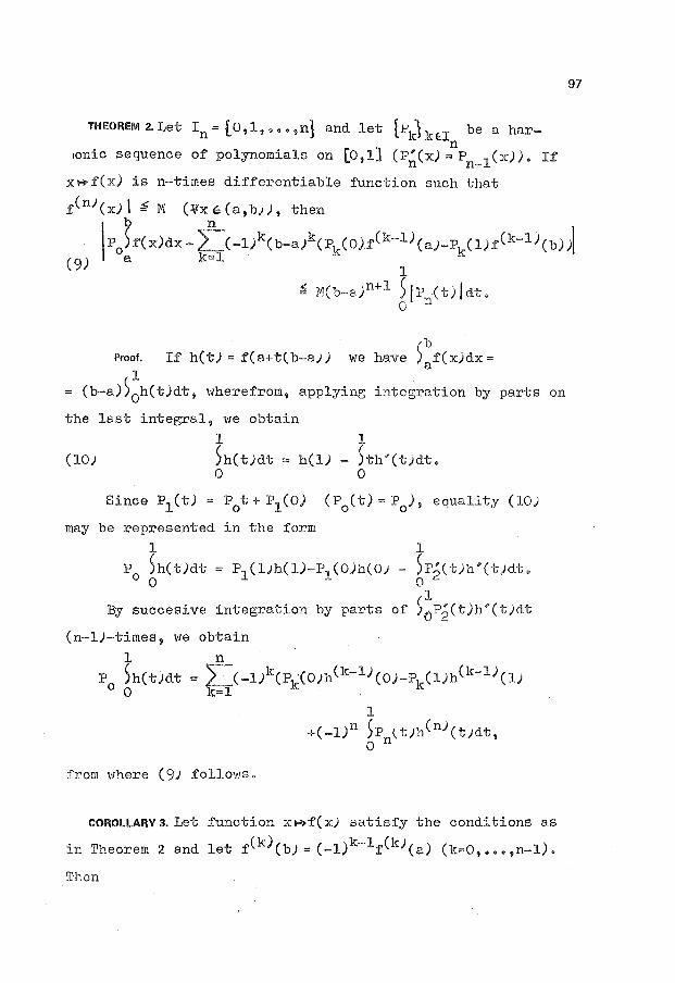
THEOREM2.Let In=[O,l, ••• ,nJ and let fPkllcH be a harn
tonic sequence o:f polynomials on [o, 1] (P'(x) = P 1(x)). If n n-
XI-'P'f(x) is n-times differentiable function such that
97
1:rCn) (x) I ~ M (¥x E: (a, b;), then
\P J:f(x)dx- Ln ( -l)k(b-aJk(Pk(O).:rCk-l) (aJ-Pk( l)f(k-l) (b);\
(9) a k=l 1
~ M(b-a)n+l )jP {tJidt. C n
Proof. I:f h(tJ = f(a+t( b-a)) we have )~f(x)dx = 1
(b-a))0h(t)dt, \·Jherefrom, applying integration by parts on
the last integral, we obtain
1 1
(10) )h(t)dt = h(l) 0
- ~th'(t)dt. 0
Since P1(t)
may be represented in the form
1 1
P0 ~h(t)dt = P1 (1Jh(l)-P1(0)h(0) - ~P2(t)h'(t)dt.
1 By succesive integration by parts of ) 0P2(t)h'(t)dt
(n-1)-times, we obtain
1 n P
0 )h(t)dt = LC-l)k(P ·(O)h(k-lJ(O)-P (l)h(k-l)(l) 0 k=l k . k
1 +(-l)n )p \t)h(n)(t)dt,
0 n
from where (9J :follows.
COROLLARY a. Let function x t-'>:f( x) satisfy the conditions as
(k) )k-1 (k) ) ) in Theorem 2 and let :f (b)= ( -1 f (a (k=O, ••• ,n-1 •
Th0n
8
(11) !tf(x)dx t ~ ~1~b-a)n+l. a I 2 (n+l)!
To nrove this, tat:e P (tJ =- --\- (t -1/2)11, i"n Theore' ::,. n n.
REMARK3. ~:ce inequality (ll) is obtained in [6] with some-
V!hat stricter conditions for f.
REFERENCES
1. ANON: Problem E ?155· Ame:r. Math. Monthly 76 (1969), 188.
2. ZAIDHAl~ S.: Problem E 2622. Ibid. 83 (1976), 74-0-74-l.
3. TORCIUl:YSKY A.: Solution of the Problem E 21;:15. Ibid. 76
( 1969)' 114-2-114-3.
4-. I'JITRINOVIC~ D.S. (In cooperation with P.M. VAEIC): Analytic
Inequalities. Ber1in-Heiilelberg-New York, 1970.
5· VASI0 P.B. and MILOVANOVIC G. V.: On an inequality of Iye
ngnr. Uni v .Beograd. Publ.Elektroteh.Fak.Ser.!11at .I'iz. No
54-l~-576 (1976)' lC:-24-.
6. ~ULOVANOVIC G. V. and PECARI( J .E.: Some considerations on
Iyengar's inequality and some related applications. Ibid.
No 54-4-576 (1976), 166-170.
7. !ULOVANOVIC G. V. : 0 ncki!:i funkcione,1nim ne jeclnakostima.
Ibid. No 599 (1977), l-59.
8. KA:::U.lftATA J.: 0 prvom stavu srcclnjih vrednosti odredjenih
integra1a. G1as srpske kraljevske akademije CLIV Beot;rRd
(1933), ll9-H4-. 0
9. AS LUND N. : The fundamental theorems of information theory
II. Nordislc. f'1at. Tidskr. 9 (1961), 105.
Numerical Methods and
Approximation "fheory
Nis, September 26-28, 1984
CLASSIFICATION OF FORMULAS FOR N-DIMENSIONAL POLYNOMIAL INTERPOLATION
Dusan V. Slavic, Milorad J. Stanojevic
lSTRACT:
e increased significance of interpolation in complicated computer calcution of the function values for either one or several variables imposes the ed for evaluation of the possibilities and the efficiency of some interpolam formulas. The paper gives a classification of the formulas for polynoial interpolation in the n-dimensional space ( n = 1, 2, 3, .•• ) •
ASIFIKACIJA FORMULA ZA N -DIMENZIONALNU POLINOMSKU INTERPOLACIJU. Povecani znacaj interpolacije u komplikovanim kompjuterskim izracunavanjima vrednosti funkcije jedne i vise promenljivih namece potrebu za vrednovanjem mogucnosti i efikasnosti pojedinih interpolacionih formula. U radu je data klasifikacija formula za polinomsku interpolaciju u n-dimenzionalnom prostoru ( n = 1, 2, 3, ••• ) •
CLASSIFICATION
The classification is hierarchical with the following order of priori
ties: according to the number of space dimensions as the most important
criterion, according to the related number of nodes for the same number
of space dimensions, according to the positions of the nodes and in relation
to the algebraic accuracy when the above three. conditions are satisfied.
The algebraic accuracy of each formula is expressed by a polynomi
al, having coefficients with arbitrary values, so that the formula is exact
for that polynomial ( not only approximate ) .
Known formulas are transformed in this paper in order to enable
the classification.
In applications, the cases with symmetric node positions are of spe
cial interest. In the notation used in this paper the subscripts with the func
tion denote node positions.
99
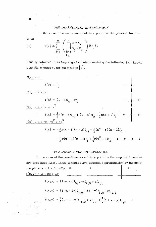
100
ONE-DIMENSIONAL INTERPOLATION
In the case of one-dimensional interpolation the general formu-
la is
( 1)
usually referred to as Lagrange formula containing the following four known
specific formulas, for example in [ 1].
f(x) = a
f(x) f0
f(x) a + bx
f(x)
f(x)
f(x) = ( 1 - x)f0
+ xf1
2 a+ bx +ex
1 2 1 f(x) = -zx(x- 1)f_
1 + (1- x )f
0 + 2x(x + 1)f
1 2 3
a+ bx +ex + dx
+ + +
f(x) = -~x(x -1)(x- 2)f_1
+l(x2
- l)(x- 2)f0
j 1 1 2 -- x(x + 1)(x- 2) f + -x(x - 1)f
2 1 6 2
TWO-DIMENSIONAL INTERPOLATION
In the case of the two-dimensional interpolation three-point formulas
are presented first. These formulas are function approximation by means o:
the plane z = A + Bx + Cy. t 0 I I 1111
f(x,y)=A+Bx+Cy -f- ---+-- +--f(x,y) (1 -x -y)fo,o +xf
1,0
+ yf011
f(x,y) = (1 -x- 2y)fo,o + (x + y)£1
,0
+yf_1
,1
f(x,y) '1 1
= 2 ( 1 - X - y )f_1 10 + yf0
11 + 2( 1 + X - y )f1
10
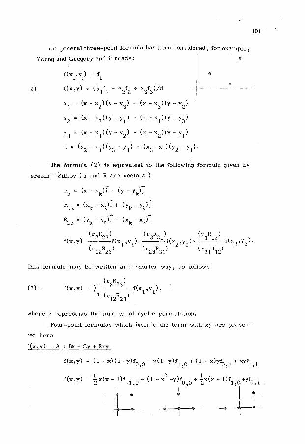
.Lhe general three-point formula has been considered, for example,
Young and Gregory and it reads:
f(x. ,y.) = f. 1 1 1
2) f(x,y) = (a1
f1
+ a2
f2
+ a3
f3)/d
al (x- x2)(y- y3) - {x- x3)(y- y2)
a2 (x-x3)(y-yl)- (x-xl)(y-y3)
a3 (x-xl)(y-y2)- (x-x2)(y-yl)
d = (x2- xl)(y3- yl) - (x3- xl)(y2- yl).
The formula (2) is equivalent to the following formula given by
.erezin - Zitkov ( r and R are vectors )
-+ -+ rk = (x- xk)i + (y- yk)j
-+ -+ rkQ. = (xk- xQ.)i + (yk- yQ.)j
-+ -+ RkQ. = (yk- yQ.)i - (xk- xQ.)j
101
(r2R23) (r3R31) 1
(r1R12) f(x,y)=---f(x
1,y
1)+ f(x
2,y21 + --- f(x 3 ,y3).
(r12R23) (r23R31) (r31Rl2)
This formula may be written in a shorter way, as follows
(3) f(x, y)
where 3 represents the number of cyclic permutation.
Four-point formulas which include the term with xy are presen
ted here
f(x ,y) A + Bx + Cy + Exy
f(x, y) (1- x)(l -y)fo,o + x(l -y)f1 , 0
+ (1- x)yf0 , 1 + xyf1 , 1
f(x, y) ..!. x (x - 1) f ( 1 2
) f 1
( ) f f
2 +=. -~2xx+~ ·ro:·
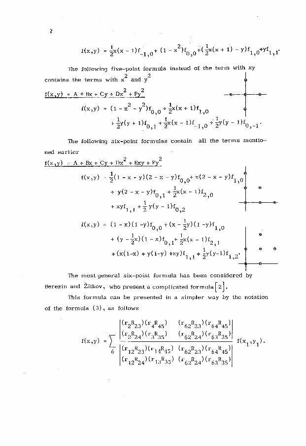
2
1 2 1 ) ) f(x,y) = -x(x- l)f + (1- X )f0
f\+(-2x(x + 1 - Y £1 0+yf1 1• 2 -1 ,o . ,v ' '
The following five-point formula instead of the term with xy
. h 'h 2 d 2 contams t e terms w1t. x an y
f(x,y) 2 2
A + Bx + Cy + Dx + Fy
f(x,y) =
The following six-point formulas ·contain all the terms mentio
ned earlier 2 2
f(x,y) A+ Bx + Cy + Dx + Exy + Fy
f{x,y) 1 = -(1- X- y){2- X- y)f + x(2- X- y)f 2 o,o 1,0
1 + y(2 - x- y)f + -x(x- l)f 0,1 2 2,0
1 +xyf1 1 +2y(y- 1)fo 2 , ,
f(x,y) 1 (1- x)(1 -y)f + (x- -y)(1 -y)f o,o 2 1,0
1 1 + (y - 2x)(1- x)f
0,1+ 2x(x- 1)f
2,1
1 +(x(1-x) + y(1-y) +xy)£
1,1
+ 2y(y-1)f1 , 2•
The most general six-point formula has been considered by
Berezin and Zitkov, who present a complicated formula [ 2].
This formula can be presented in a simpler way by the notation
of the formula ( 3) , as follows
l(r 2R23) (r l4s) (r62R23)(r64R45)1
f(x, y) =[ (r2R24)(r3R35) (r62R24)(r63R35)
f(x1,y1).
6 (r12R23)(r14R45) (r6ZR23)(r64R45)
(r12R24)(r13R35) (r6l24)(r63R35)
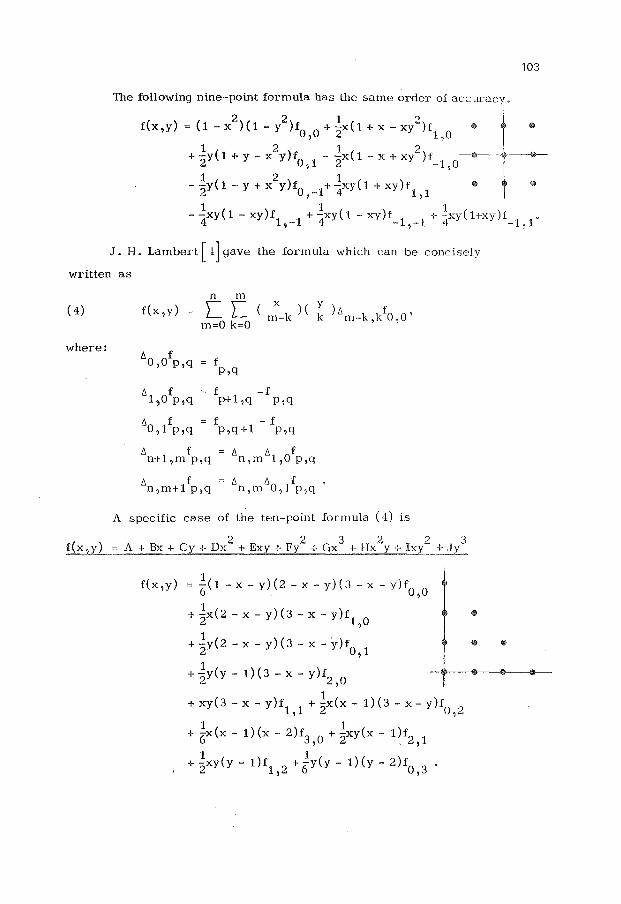
103
The following nine-,point formula has the same order of accuracy.
2 2 1 ') f(x,y) = (1- x ){1- y )f
0 0 + -
2x(1 + x- xy~)f
' 1,0 1 2 1 2
+ -y( 1 + y - x y)f - -x( 1 - x + xy )f 2 0,1 2 -1,0 1 2 1
- Zy(l- y + x y)f0 ,_1+4xy(1 + xy)f
1,1
1 1 . 1 --xy(1-xy)f +-xy(l-xy)f +-xy(1+xy)f •
4 1,-1 4 -1,-1 4 -1,1
J. H. Lambert [ 1] gave the formula which can be concisely
written as
n m ( 4) f(x, y) C C < r:;_k )(
y )6 f
k m-k,k o,o' m=O k=O
where: /':. f o,o p,q f
p,q
/':. f f -f 1 ,o p,q p+1,q p,q
/':. f o, 1 p,q f - f p,q +1 p,q
/':. f n+l ,m p,q
/':. /':. f n,m 1 ,o p,q
/':. f n,m+1 p,q
/':. /':. f n,m o, 1 p,q
A specific case of the ten-point formula ( 4) is
f(x,y) 2 2 3 2 2 3
A + Bx + Cy + Dx + Exy + Fy + Gx + Hx y + Ixy + Jy
f(x,y) = _!(1- X- y)(2- X- y)(3- X- y)f 6 . o,o
+ _!X ( 2 - X - y) ( 3 - X - y) f 2 1 ,o
+ .!y(2- X- y){3- X- y)f 2 o, 1
+ _!y(y- 1){3- X- y)f 2 2,0
+ xy(3- x- y)f + lx(x- 1)(3- x- y)f 1,1 2 0,2
1 1 + 6x(x- 1)(x- 2)f
3,0
+ 2xy(x- 1)f2
,1
+ lxy(y- 1)f + .!y(y- 1)(y- 2)f 2 1,2 6 0,3

F. B. Hildebrand gives the following formula
2 2 3 f(x,y) = A+ Bx + Cy + Dx + Exy + Fy + Gx
2 2 3 3 3 + Hx y + Ixy + Jy + Lx y + Nxy
f(x,y) = ~(1- x)(1 -y) [2 + x(1 -x) + y(1- y)] f0
,0
+ ~x(x- y) [2 + x(1- x) + y(1 -y)] f1
,0
+ ~xy [2 + x.(1 -x) + y(1- y)] f1
,1
+~(1-x)y[2+x(1 ~x) +y(1-y)] f0
,1
+ ..!x(x -1 )(x- 2)(y:.. 1)f 6 -1,0 1
+ -(x -1)y(y -1)(y- 2)f 6 o,-1 1
+ 6xy(y- 1) (2 - y)f1 1
_1
1 2 + -x(1- x )(y -1)f
6 2,0 1 2 1 2
+c;x(x -1)yf211
+ 6 xy(y
THREE-DIMENSIONAL INTERPOLATION
For interpolation in the three-dimensional space the following
formulas are given
f(x,y,z) = a
f(x,y,z)
f(x,y,z) = f o,o,o
f(x,y,z) ( 1 -X - y - z)f0 0 0 + xf1 0 0 + yf0 1 0 ' ') ' ' ' '
+ zfo 0 ' '1
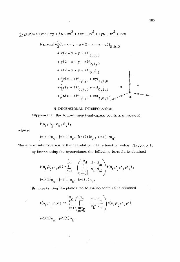
2 2 2 r(x,y,z)=a+Sx+yy+oz+EX +z;xy+ny +eyz+tz +Kxz
where:
1 f(x,y,z)= 2(1- x- y- z)(2- x- y- z)f
0 0 0 ' , + x(2 - x - y - z)f
1,0,0
+ y(2- x- y- z)f o, 1 ,o
+ z(2- x- y- z)f 0,0,1
1 + 2x(x- 1)f2,0,0 + xyf1,1,0
1 +2y(y- 1)fo 2 o + yzfo 1 1 , ' , ,
1 + 2z ( z - 1) fo o 2 + xzf1 o 1.
' , ' ,
N -DIMENSIONAL INTERPOLATION
Suppose that the four-dimensional-space points are provided
f(a., b., c1
, dJ, 1 J ( JC
105
The aim of interpolation is the calculation of the function value f(a,b,c,d).
By intersecting the hyperplanes the following formula is obtained
nd
f(a.,b.,c1 ,d)~[
l J ( t=l
i=1(1)na' j=l(l)nb'
By intersecting the planes the following formula is obtained
n (n c c f(a.,b.,c,d) ""' L n
1 J k=1 m=1
m;ik
i=1(1)na' j=1(1)nb.

By intersecting straight lines the following formula is obtained
i=1(1)n • a
By applying the mentioned Lagrange formula ( 1) it can be obtained
n ( n a a
f(a,b,c,d) = !;_ rCl mn
_a_-_a_m_) f(a. ,b,c ,d). a.- a 1
1 m
For the dimension number greater than four, the beginning of the pro
cedure is analogous, and the end is the same as given in the above algorithm.
When dealing with the interpolation having a larger number of points
in then-dimensional space the simplicity of notation is important.
A more extensive work on formulas with a larger number of points is
expected in future. The aim of this paper is not to deal with the formulas
based on a larger number of pointsl because the application of these formu
las is smaller due to larger computation procedures. Due to the limited
length of the paper some more complex, but useful formulas, are not included
For this reason the paper contains only the most important formulas
for computer calculation.
G. Alikalfic, A. Djordjevic, A. Fiser-Popovic, D. T. Jovanovic,
D. S. Mitrinovic have read this paper in manuscript and have made some
valuable remarks and suggestions.
REFERENCES
1. ABRAMOWITZ M., STEGUN I. A.: Handbook of Mathematical Function, National Bureau of Standars, New York 1964.
2. BEREZIN I. S., ZITKOV N. P.: Numericka analiza (Numericke metode), Naucna knjiga, Beograd 1963.
3. BUCKINGHAM R. A.: Numerical Methods, Pitman and Sons,London 1962. 4. DAVIS H. T. : Tables of the Higher Mathematical Function, The Principia
Press, Bloomington, Indiana 1933. 5. HILDEBRAND F. B.: Interpolation to Numerical Analysis, McGraw-Hill,
New York 1974. 6. STEFFENSEN J. F.: Interpolation,Chelsea Pub.Company,New York 1950. 7. YOUNG D. M., GREGORY R. T.: A Survey of Numerical Mathematics,
Vol. I, Addison - Wesley Series in Mathematics, Reading 1972.
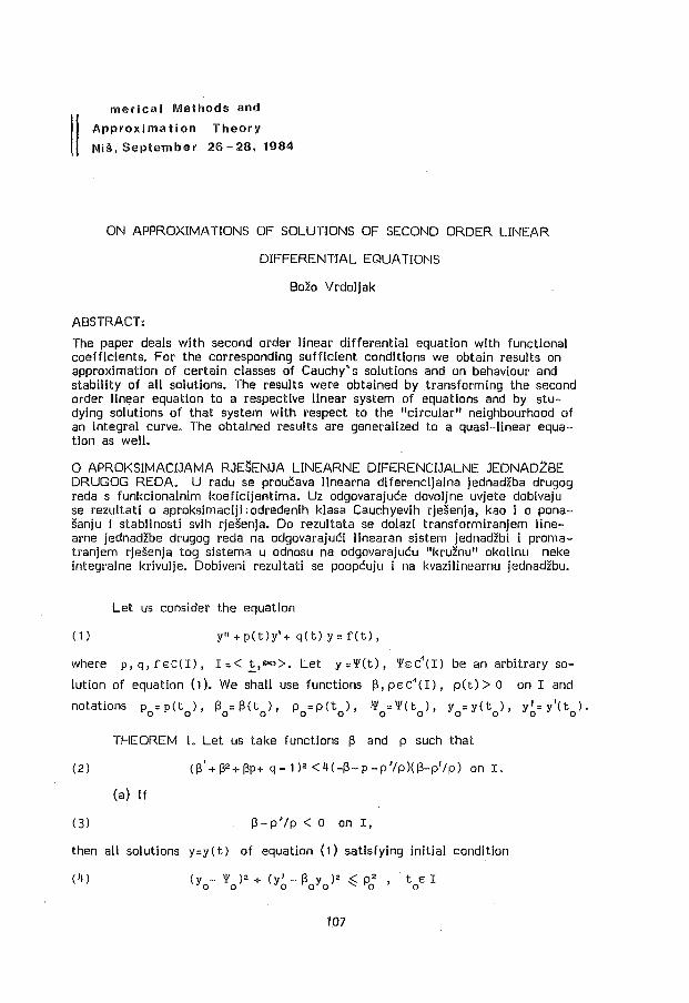
merical Methods and
II Approximation Theory
Nis, September 26-28, 1984
ON APPROXIMATIONS OF SOLUTIONS OF SECOND ORDER LINEAR
DIFFERENTIAL EQUATIONS
Bozo Vrdoljak
ABSTRACT:
The paper deals with second order linear differential equation with functional coefficients. For the corresponding sufficient conditions we obtain results on approximation of certain classes of Cauchy's solutions and on behaviour and stability of all solutions. The results were obtained by transforming the second order linear equation to a respective linear system of equations and by studying solutions of that system with respect to the "circular" neighbourhood of an integral curve. The obtained results are generalized to a quasi-linear equation as well.
0 APROKSIMACIJAMA RJESENJA LINEARNE DIFERENCIJALNE JEDNAD.LBE DRUGOG REDA. U radu se proucava linearna diferencijalna jednadzba drugog reda s funkcionalnim koeficijentima. Uz odgovarajuce dovoljne uvjete dobivaju se rezultati o aprokslmaciji 'odredenih klasa Cauchyevih rjesenja, kao i o ponasanju i stabilnosti svih rjesenja. Do rezultata se dolazi transformiranjem linearne jednadzbe drugog reda na odgovarajuci Iinearan sistem jednadzbi i promatranjem rjesenja tog sistema u odnosu na odgovarajucu "kruznu" okolinu neke integralne krivulje. Dobiveni rezultati se poopcuju i na kvazilinearnu jednadzbu.
Let us consider the equation
(1) Y"+p(t)y'+ q(t)y::f(t),
where p,q,fEC(I), I=<!_,CXl>. Let y:'Y(t), 'YE:C4(I) be an arbitrary so
lution of equation (1). We shall use functions (3,pEC'(I), p(t)> o on I and
notations p0:p(t
0), f3
0=f3(t
0), p
0:p(t
0), ·'¥
0='Y(t
0), Y
0=y(t
0), Y~=y'(t0 ).
THEOREM
(2)
(a} If
(3)
then all solutions
(4)
I. Let us take functions (3 and p such that
( (3 1 + (32 + (3p + q - 1 )2 < 4 ( -(3- p - p 'I p )( (3- p1 I p) on I.
(3-p'lp < 0 on I,
y:y(t) of equation ( 1) satisfying initial condition
107
t E I 0

sausfy also condition
(5) \y(t) -'l'(tll < p(t) for every t> t0
•
(b) If
(6) 13- p' /p > o on I,
then problem ( 1)-( 4) has at least one solution satisfying condition ( 5).
Proof. For equation ( 1 ) let us introduce the substitute
(7) y'= x+13(t)y,
where x = x ( t) is a new unknown function. Equation ( 1) is transformed to the
system of equations
x' = -(13 + p) x-. <13'+ 132+13p+q)y + f (8)
Y1= X+i3Y.
Let K::{ (x,y,t): x::<p(t), y::'l:'(t), tEl}, where <pEC.(I), cp(t0
):::0
is an integral curve of system (8). Let Q = R2 x I and
W::: {<x,y,t)EQ : p\t)[(x-cp(t))2
+(y -'l'(t))2)< 1 J
be open sets. Let :< t) be a tangential vector or the integral curve ( x(t),
y(t), t) of system (8) in points of surface ow (ow:::c.tw'\w), and let v(t)
be vector of external normal on surface a w, i.e. -2 -2
't:(t):::(x'(t),y'(t),1), v(t)::((x-<p)p ,(y-'l')p ,
- [ (x -fll)2p' +(x-cp)pcp'+(y-'1')2 p'+(y-'l')p'l''] p3). Let us consider now the scalar product P ( t) = ( 1:1 v) in the points of
surface () w. We have -2 -2
P(t):(-13-p -p'/p)(x-<p)2 p +(13-p'/p)(y-'!') 2 p + (9)
+( 1-13'-132-13p-q) (x- cp) p-1 (y- '!:') p1 •
Let us note that P(t) is a quadratic symmetric form
where a 11 :: -13-p-p'/p, a 12= a 21 =(1-13'-j32-13p-q)i2, a 22= 13-p'/p,
( 10) X::(x-<p)p-• , Y: (y-'l')p1,
Moreover, it is sufficient to note the following.
(a) Conditions (2) and (3) grant conditions -a 11 >o, a11
a22-a;2
>o on
I, and according to Sylvester's criterion it follows that P(t)<O on I. Rela
tion P(t) < 0 means that set &w Is a set of points of strict entrance for

integral curves of system (8) with respect to sets w and Q • Consequently,
all solutions of system (8) satisfying initial condition
X~+ ( y 0 -IJI 0 )2 ~ p~ ' t 0 E I
(x0
= x( t0
)) satisfy also condition 2 2
(x{t) -QJ(t)) +(y(t)-IJI(t)) < p2 (t) for every t> t0
•
Since, in view of (7), x = y 1 - 13 y all solutions of equation ( 1) satisfying
0 0 0 0
initial condition ( 4) satisfy also condition (5).
(b) Conditions (2) and (6) grant conditions a11
>O, a11
a 22-a?12> 0 on
I, and it follows that P(t) > 0 on I. Tbus 'a w is a set of points of strict
exit of integral curves of system (8) with respect to sets w and Q • Henc!'!,
according to retraction method (l4J), there exists at least one integral curve
of system (8) which belongs to set w for every t EI. Consequently, problem
( 1)-( 4) has at least one solution satisfying condition (5).
Let us note that conditions of Theorem 1 are simplified if functions 13
and p are taken in a special form.
COROLLARY (p(t):: r). (a) ( 13(t): -1) If
p > 1 , 0 < p - 2 yp::1 < q < p + 2 yp::-1 on I ,
then all solutions of equation ( 1) satisfying initial condition
( 2 I 2
Yo-'¥ o) + (Yo+ Yo) .::; r 2 '
where r is a positive constant, satisfy also condition
( 11 ) I y(t)- IJI(t) I < r for every
(b) (13(t) = 1) If
t > t 0
p < -1, 0 < - p -2 .y:p::j < q <- p + 2 v::r;-:::1 on I ,
then at least one of solutions of equation ( 1) 'which satisfy initial condition
2 I 2 (yo-'l'o) +(yo-yo)~ r2
satisfies also condition ( 11 ).
COROLLARY 2 (13(t):: 0). Let
(q-1)2 < 4(p+p1/p)p 1/p ani.
{a) If p' > 0 on I, then all solutions of equation ( 1) which satisfy ini
tial condition
( 12) 2 .?.
(y - '¥ ) '+ y 1 < p02 , t E I
0 0 . 0 0
109
satisfy also condition ( 5) •
(b) If p 1 < o on I, then problem ( 1 )-(12) has at least one solution sa
tisfying condition (5 ).
COROLLARY 3 (f3(.t):: -p(t)). Let
( q- pt - 1) 2
< 4 ( p + p' /p )p1 I p on I.
(a) If p1 > o on I, then all solutions of equation ( 1) satisfying initial
condition
2 I 2. ( 13) (yo-'l!o) +(yo+poyo)· ~Pi)
satisfy also condition (5 ).
(b) If p1 > o on I, then problem ( 1 )-(13) has at least one solution
satisfying condition (5 ).
( 14)
or
( 15)
THEOREM 2. (a) If there exist functions f3 and p such that
2f3+ p ~ 0' \ f31+ f3 2+ f3p+ q- 1 \< 2·( f3+ p +p'/p)
on I, then statement (a) of Theorem I holds true.
(b) If there exist functions f3 and p such that
2f3+p ~ o, \ f3~f3 2 +f3p+q-1\< 2(-f3-p-p1/p)
or 2f3+p ~ o, lf3
1+f32 +f3p+q-1\< 2(f3-p1/p)
on I, then statement (b) of Theorem I holds true.
Proof. Let us use here the first part of the proof of Theorem I until
the formation of the scalar product P( t) according to formula (9). We shall
also use notations (10). It is sufficient to note that the following estimates
for P(t) hold true.
(a) Since ab~ (a2 +b2)/2 for every a,be:R, on ow it is valid
P( t) ~ ( -f3 -p- p1/p) X2 +( f3 -p1/p) Y2+11- f31- f32 -f3P- q I. (X2 + Y2) /2 = P( t).
In view of (14) on 'aw it is valid
P(t) = (-f3-p-p1/p+ l1-f31-f32 -f3p-q\!2)(X2 +Y2 )+(2f3+p) Y2 =
= (- f3 -p- p'tp + r 1- f3'-f3 2 -f3p- q 1,2 >+<2f3+ p )Y2 < o.
Moreover, in view of (15) on ~w it is valid
P(t) = (f3-p 1/p+ \1-f31-f3 2 -f3p-q\!2)- (2f3+p)X2 < 0.
(b} Here it should be noted tf\at on ;) w
P( t) :? (- fl- p - p 1/P) X2 + ( fl-p'!p) Y•- I 1 - fl1- fl 2 - i3p-q \ (X• + Y• ) I 2 = !: ( t)
nd that !:(t} > 0.
Conditions of Tneorem 2 are simpfffied if functions fl and p are taken
in a special form. For example fl(t):::0,-1, 1' p(t):p0e-s(t-to>, se:R.
Using the obtained results and the known properties valid for the linear
jjfferential equation, we can draw the following conclusions related to the
~uestions of stability and approximation of solutions of equation (I).
I. If function p is bounded on I, then in cases (a) of all given state
nents we have stability of all solutions of equation (I) with the function of
;tability p (t5]). If p(t)-o, t_,.oo, we have asymptotic stability of all so
utions with the function of stability p.
2. If p(t)-J> oo , t-=, then in cases (b) of all given statements we
1ave instability of all solutions of equation (I) with the function of instability
3. Considering the approximation of certain classes of solutions the re
sults given in cases (a) with the bounded function p are very significant. Ap
proximation is particularly good when p ( t >- o, t _,. oo. In that case we have
precise asymptotic behaviour of certain Cauchy's solutions. Consequently it
should be noted that conditions of Theorems I and 2 do not change if instead
of function p ( t) we take function c p ( t) , where c>o is an arbitrary consta"nt.
111
In the case of a homogeneous equation (f(t) =o) it is interesting to con
sider the behaviour of solutions in the neighbourhood of a trivial solution
y(t): o (case 'l'(t):O).
Remark. Statements of Theorems I and 2 are completely valid also for
a quasi-linear equation
Y"+p(y,t)y 1 +q(y,t)y:f(y,t),
. where functions p, q and f satisfy the conditions necessary for the existence
and uniqueness of solutions on R><I, only if the respective conditions of Theo
rems I and 2 (p:p(y,t), q:q(y,t)) hold true on aw'.
Example I. All the solutions of the Bessel's equation
which satisfy the initial condition
(y -'1' )2 + (y'+y /2t )2:;:; p2' o o ·o o o o
where .!:_>\>..2 -1!4\!(1-2s), sER, O<s<1/2, then also satisfy condition
I y{t) -'l'(t) \ < p (t /t)5 for every t >t •
0 0 0
For example, for X.= 1/2, 'l'(t): 0 all solutions of the Bessel's equation
satisfying initial conditions y = 0, 1 y 1 \ ~ p , t > o satisfy also condition 0 0 0 0 s .
\y(t)\ < p (t /t) for every t>t • Let us note that for X.= 1/2 Bessel's equ-o 0 0
at ion has a general solution y = ( c1 cos t + c2sin t) Nt. The proof of this result follows from Theorem I when 1:\(t) = -1/2t,
p{t) :p (t /t) 8•
0 0
Example 2. Let us take equation
Y"+p(t) (y 1+y)+q{t)y:d(t),
where p(t) ~2, \q(t)\<2(1~s), sER, O~s < 1, on I, t> 0. All solu
tions of this equation which sastify the initial condition
also satisfy condition
\y (t) -'l'(t) \ < -s(t-t ) Poe o
t 8I 0
for every t> t0
•
It is interesting to consider the case f{t):: o, 'l'{t) ::0.
This result follows from Theorem 2 when 1:\(t) = -1 , p(t) :p0e-s(t-to).
REFERENCES
I. HATVANI L.: On the asymptotic behaviour of the solution of (p(t) x')1+
q(t) f{x) = o. Publicationes Math. Debrecen, 19 (1972), 225-237.
2. NEJMAN F. : Teorija global' nyh svojstv obyknovennyh linejnyh differencial'
nyh uravnenij n-go porjadka. Differenc. uravnenija, 19 ( 1983), 799-808.
3. READ T. T. : Second-order differential equations with small solutions.
J. Math. Anal. Appl. 77 (1980), 165-174.
4. VRDOLJAK B. : Curvilinear "tubes" in the retraction method and the be
haviour of solutions for the system of differential equations. Mat. vesnik
4 (17) (32) (1980), 381-392.
5. VRDOLJAK B. : On behaviour of solutions of system of linear differential
equations (in preparation).
Faculty of Civil Engineering, University of Split,
V.Maslese bb, P.O. Box 389, 58000 Split, Yugoslavia

Numerica I Methods and
Approximation Theory
Nis, September 26-28, 1984
ON HYPOTHESIS TESTING IN SPLINE REGRESSION
K. Sur! a, E. Nikolic, Z. Lozanov
ABSTRACT:
Algorithm given in [21 for deter-ming the number and the position of knots of the spline function is modified according to statistical tests in [B] for fitting the cubic spline regression. Several theorems conected with testing continuity of the third derivative are proved.
0 TESTIRANJU HIPOTEZA U SPLAJN REGRESIJI: AZgoritam datu [21 za odredji~anje broja i pozicija avorova splajna je modifikovan u skZadu sa statistiJkim testovima datim u [BJ za'fonniranje kubne spZajn regresije. Dokazane ~u neke teoreme vezane za testiranje hipoteza o neprekidnosti tredeg izvoda.
1. In modeling, curve fitting or recovering functions contaminated
by noise, the problem of determining the minimal number and optimal positi
ons of knots is still open, although some attempts had been made, see [51,
[10], [11j. In [2], [3] an algorithm for automatic determination of the
number of knots and their positions for fitting a least square spilne of
k-th degree is given. The objectives are (i) the given values of dependent
variable should be fitted closely enough, (ii) the approximating spline sho
uld be smooth enough, in the sence that the discontinuities in its k-th de
rivative are as small as possible •. Also, it Is presumed that the data are
not contaminated by noise. In fitting spline regression curve to discrete,
noisy obsrevations, besides the problem of c~oice of knots, occurs the pro
b) an of their statistical testing. These problems are investigated in [1],
[4], [7], [8], [10], [11]. Hypothesis testing in B-spline regression is
investigated in [8] and [11].This paper is an attempt to applicate the
results obtained in [2] to B-spllne regression, and to mcdify the algorithm
in [2] according to the :>tatistical tests in [8].
2. Given the measured function values yq, at the points xq' q=1 , ... ,m,
xq<xq+ 1 , coisider the model
( 1) y
- tB~3 (x1) ... B g.(x1 j X - • • . .
B 3
(x ) ... B (x ) - m g m
E: = [['] m

~··
srvN(O,cr 2I), B. (x) are B-splines functions of the third degree on the grid I
a= A. 0 <A. 1 <.~.<A.9 <A.g+l= b, with additonal knots x_3
=A._2 =A._ 1=a, b~\g+Z
\ 3=\ 4• We suppose that there must be at least one·s.ubset of g+4
g+ g+ strictly increasing values x , (i=-3, .•. ,g) such that q. (2) x 4<A.ro::x
1 (condition Schoenberg and Whitney).
qi- qi
The approximation criterion is as In [2] g g
Minimize E1
(.E 3c.a. ) 2
, subject to the constraint q= I=- I I ,q
(3) m g ~ 1 ~Y -. E
3c. B •. (x ) ) 2 < s · q- q 1=- I I q
where S is given, nonnegative constant (smoothing factor).
(4) a. =B.(\ +0) - B.(\ -0), (q=l , .•. ,g), (i=-3, .•. g). I ,q I q I q g
We remark that our spline function S(x) = .1:: 3c.B. (x) becomes a single
g I>=- I I
polynomial on [x ,x J if . E3C.a, ,=0, (j;=q+1 , ... ,r-1), a:c;x ,x ~b. q r 1 =- 1 1 , J q r
In [2] it is shown that problem (3) has a solution and that the algorithrr
given there I eads to the number of knots wich
m gk F(n) = E1 ("- .E
3c. (p)B. (x )) 2 .$ S,
"' q= "q I=- I I q
where p- 1 is Lagrange's multiplier of problem (3). Also, the relation be
tween the parameter p and the number of knots Is given. So, for p= we ge1
the least square spline, and for p=O we get the 1 east square polynomial.
3. For testing the continuity of the third derivative at the knot
Aj we test the following hypothesis (see [8]): g
H0
.E 3c. (B. (A.+O) - B.(/. .-0)) 0
1=- I I J I J
We use the statistics
( 1 'C) 2 (1 .. (XX') - 11} - 1 F (m-g-4) or F =
y ( I -X (XX' ) - 1 X' ) y
2
(!.::.fl. V ( 1 'C)
A
where V(l'C) is estimated variance of linear combination t'C, l'=(a_3,j'.,
a 2
., ... ,a .). Un'der null hipothests F has Fisher distribution F1 4• ,.. +J q ,J ,m-g-
Using the fact that the linear combination which is tested is contrast,
!see [8]), it is enough toevaluateg+3 components of vector l. If hypo
thesis H0
is accepted, we shall say that knot \. is statisticaly not si-J -·
gnificant. Statisticaly not significant knots we shall denote by\,, - J U=1 , ... ,g).
4. Denote the spline function with knots \,(j=O, •.. ,g+l) by S (x). J g
The idea of our algorihtm is: Determine the least square spline s0
(x) (si·
ngle polynomial). If the sum of squares of residuals for s0
(x) is less
than S, s0 (x.) is the solution to our problem. If not, we determine
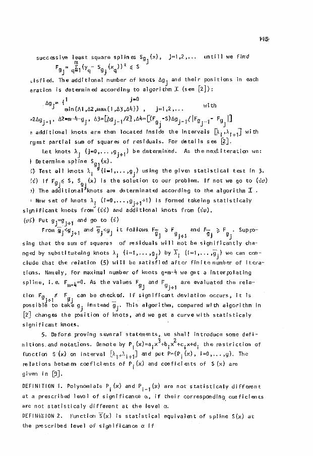
successive least square splines Sg,(x), j=1,2, ... untill we find
F9
= ~1 (y- sg (xq}) 2 ~ s J j q= q j
dsfied. The additional number of knots Ligj and their positions in each
eration is determined according to algorithmi (see [2]):
1 j=O Lig.= {
J min{Li1,Li2,max{1 ,Li3,Li4}} , j=1,2, ... with
=2LigJ_ 1 , Li2=m-4-gJ, LiJ.=IJigJ_,J2J ,Li4=[(FgJ -s)LigJ_ 1f.IFgr 1- F9J IJ
a additional knots are then located inside the intervals [A. 1 ,A.i+,J with
rgest partial sum of squares of residuals. For details see[?].
Let knots A.. (j=O, ... ,g. 1) bedeterminied. As thenextiteration we:
J J+ f Determine spline sg:(x).
~'Test all knots A.. ~(i=1, ... ,g.) using the given statistical test tn 3. I J
(i) If Fgj~ S, Sg; (x) is the solution to our problem. If not we go to (iv)
J) The addi tional:lknots are de terminated according to the algorithm I
1 New set of knots A.r (i=O, ... ,gj+l+l) Is formed takeing statisticaly
significant knots fromJ(ii) and additional knots from (iv).
(vi) Put g.=g. 1
and go to (i) J J+
From g.<g. 1
and g.<g. i.t fo.Jlows, F- ~ F and F- ~ F . Suppo-J J+ J J gj gj+l gj gj
sing that the sum of square!:' of residuals will not be significantly cha
nged by substituteing knots A.. (i .. J, ... ,g.) by X. (i=l, ... ,g.) we can con-I J I J
elude that the relation (5) will be satisfied after finitenumber of itera-
tions. Namely, for maximal number of knots g=m-4 we get a interpolating
spline, i.e. F _4=0. As the values Fg. and Fg are evaluated the rela-m J j+l
tion Fg ~ F can be checked. If significant deviation occurs, it is j+1 gj - '
possible to take g. instead g .. This algorithm, compared with algorithm in J J
[2] changes the position of knots, arid we get a curve with statisticaly
significant knots.
5. Befor:e proving several statements, we shall introduce some defi
nitions. and notat.ions. Denote by P. {x)=a.x3+b./+c.x+d. the restriction of , I I I I I
function S (x) on interval [A. .•.• ~''+l] and put P={P. {x), i=O, ... ,g}. The I I I
relations bet\\een coeficia1ts of P.(x) and coeficients of S (x) are I
given i n [9 J. DEFINITION 1. Polynomials Pi (x) and Pi_
1(x) are not statisticaly different
at a prescribed level of significance a, if their corresponding. coeficients
are not statisticaly different at the level a.
DEFINHHON 2. Function S(x) i~ statistical equivalent of spline S{x) at
the prescribed level of significance a if
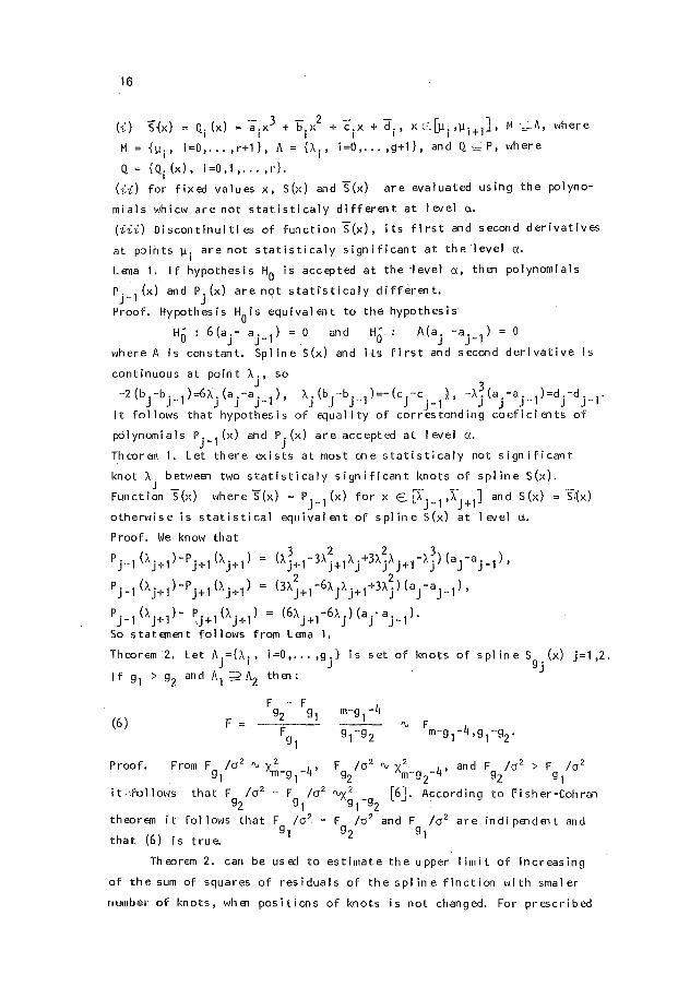
16
- ( - 3 - 2 ,-f. 1 A h (i) S(x) = Q. x) = a.x + b.x + c,x +d., x c..Lll· ,]..1.1+1 , M ·~~"• w ere
I I I I I I
M = { 11· , i =0, •.. , r+ 1 } , A = {A. , i =0, ..• , g+ 1} , and Q ·:0:: P, where I I
Q = {Q. (x), i=0,1, ... ,r}. I
(ii) for fixed values x, S(x) and S(x) are evaluated using the polyno-
mials whicw are not statisticaly different at level a.
(iii) Discontinuities of function S(x), its first and second derivatives
at points ll· are not statisticaly significant at the level a. I
Lena 1. If hypothesis H0
is accepted at the level a, then polynomials
P. 1
(x) and P. (x) are no.t statlsticaly different. J- J
Proof. Hypothesis H0
is equivalent to the hypothesis
Ha : 6(aj- aj-l) = 0 and H0. A(aj -aj_ 1 ) = 0
where A is constant. Spline S(x) and its first and second derivative is
continuous at point A., so J 3
-2(bj-bj_ 1)=6A.j(aj-aj_ 1 ), A.j(bj-bj_ 1)=-(cJ-cj_1), ->..j(aj-aj_ 1)=d(dj_ 1.
It follows that hypothesis of equality of correstonding coeficiEnts of
polynomials Pj_1
(x) and Pj(x) are accepted at level a.
Theorem 1. Let there exists at most one statisticaly not significant
knot>... between two statisticaly significant knots of spline S(x). J
Function S(x) where S(x) = P. 1 (x) for X E. 'A. 1 ,I. 1] and S(x) = s:~x) r LAJ_ J+ otherwise is statistical equivalEnt of spline S(x) at level a.
Proof. We know that 3 2 2 3
Pj-l (A.j+ 1)-Pj+1 (>..j+ 1) (A.j+ 1-3A.j+ 1>../3A.j>..j+ 1->..j) (aj-aj_ 1),
2 2 Pj_ 1 (>..j+ 1)-Pj+ 1 (A.j+1) (3A.j+ 1-6>..j>..j+1+3A.j) (a(aj_ 1),
P. 1
(>..,+ 1)- P. 1 (>... 1) = (6>...+ 1-6>...)(aj-a. 1).
J- J 'J + J + J J J-So statement follows from Lena 1.
Theorem 2. Let A.={>..., i=O, ... ,g.} is set of knots of splineS (x) j=1,2. J I J g j
1 f g 1 > g2 and A 1 2 A2 then :
(6) F =
From F /o 2 ~ v 2 4
, g1 ''111-g1-
F /o 2 ~ x2 and F /o 2 > F /o 2
92 m-g2-4' 92 91 Proof.
it.~fnllows that F /o2 - F /o 2
92 91 ~x 2
_ [6]. According to fisher-Cohran 91 92
theorem it follows that F /o 2-
91 that (6) is true.
F /o2 and F /o 2 are indi pEndEnt and g2 g1
Theorem 2. can be used to estimate the upper limit of increasing
of the sum of squares of residuals of the spline finction with smaler
number of knots, whEn positions of knots is not changed. For prescribed
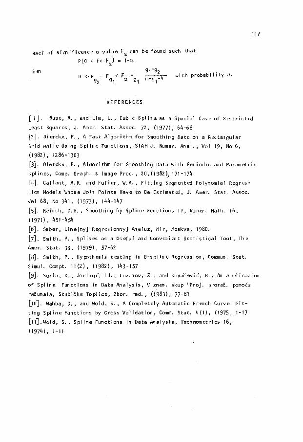
eve! of significanceavalueFacan be found such that
P{O < F< F } = 1-a. a hEll
0 <- F - F < F F 92 g 1 a g 1
REFERENCES
with probability a.
117
[1]. Buse, A., and Lim, L., Cubic Spline as a Special Case of Restricted
_east Squares, J. Amer. Stat. Assoc. 72, (1977), 64-68
[2]. Dierckx, P., A Fast Algorithm for Smoothing Data on a Rectangular
irid while Using Spline Functions, SIAM J. Numer. Anal., Vol 19, No 6,
(1982)' 1286-1303
[3]. Dierckx, P., Algorithm for Smoothing Data with Periodic and Parametric
ipl ines, Comp. Graph. & Image Proc., 20,(1982), 171-174
~4]. Gallant, A.R. and Fuller, ~/.A., Fitting Segmented Polynomial Regres
;ion Models Whose Join Points Have to Be Estimated, J. Amer. Stat. Assoc.
vdl 68, No 341, (1973), 144-147
[5]. Reinch, C.H., Smoothing by Spline Functions II, Numer. Math. 16,
(1971)' 451-454
[6]. Seber, Linejnyj Regresionnyj Analuz, Mir, Moskva, 1980.
f7J. Smith, P., Splines as a Useful and Convenient Statistical Tool, The
Amer. Stat. 33, (1979), 57-62
[8]. Smith, P., Hypothesis testing in B-spline Regression, Commun. Stat.
Simul. Compt. 11 (2), (1982), 143-157
[9]. Surla, K., Jerinuc, LJ., Lozanov, Z., and Kovacevic, R., An Application
of Spline Functions in Data Analysis, V znan •. skup "Proj. prorac. pomocu
racunala, Stubicke Topl ice, Zbor. rad., (1983), 77-81
[10]. Wahba, G., and Wold, S., A Completely Automatic French Curve: Fit
ting Spline Functions by Cross Validation, Comm. Stat. 4(1), (1975, 1-17
[11].Wold, S., Spline Functions in Data Analysis, Technometrics 16,
(1974)' 1-11

I
I
I
I
I
I
I
I
I
I

,...,merical Methods and
Approximation TheorY
Nis, September 26-28, 1984
Al PROXUJATION IN DISCRETE CONVEXITY CONES
Ivan B. Lackovic , Ljubisa M. Kocic
ABSTRACT: 'rhe necessary and sufficient conditions for positivity of linear continuous operators on a cone of convex sequences are given. The mai~ ~heor~m is base~ on ~he representation of every s~quence as a l1m1th (ln d metr1c, g1ven by (2)) of sequences uCn; given by (6). This is asdiscrete analogue of the result given in [2J, and a generalization of result from [ 1 J.
APROKSHJACIJE U DTSKRETNHl KONUSI!"JA KONVEKSNOSTI. Do bij eni su pc..trebni i d{)voljni uslovi za pozi ti vnost linearnih neprekidnih operators na konusu konveksnih nizova. Teorema se bazira na reprezentaciji svakog niza kao ~ranice (u metrici ds , koja je data sa (2)) nizova u\nJ datih sa (6). JJobijeni rezultati predstavljaju diskretnu analogiju rezultata iz [ 2 ]~ i generaliBu rezultate iz [ l L
1. ALGEBRA
In this paper, the following denotations will be used: N = {1, 2, 3, ••• ~, N
0= Nuto\, x=(x
0,x1,. •. ) =(xk)(krN
0),
S -the set of all sequences x. Further, the sequences en r S
(n r N0
) is defined by
( 1) en = ( 6 nk) (kEN 0 ) , f o, k;l n , where onk is Kronecker's. delta, onk = l l, k= n. • For two
sequences x,y r s we write· x = y if xk = yk for every k£N0 ,
and x + y = (xk + yk)(krN0), If ~rR then AX means (Axk)
(k£N )~ Thus, S together with defined operations consist a li-o
near space over the field R, with the sequences en(n£N0 ) as
a base. The sequence x = (xk) (krN
0) is convex if ll
2xn = xn+2 -
2x + x ~ 0 (nrN ). The set of all convex sequences will be n+l n o
denoted by K. It is known, that K is a cone in s. Further, let De R be a nonempty set. With F(D) we will
denote the set of all functions f: D-+ R. For the operator A: s...,. F(D) we say that it is linear if for every x,yES and
119
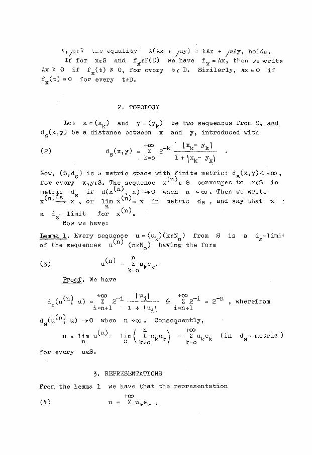
~, 1
urH ti1e equality A(/,x + 1uy) = A.Ax + ;nAy, holds. If for XES and f EF(D)
X
fx(t) ~ 0, for every
we have fx =Ax, then we write
t r D. Similarly, Ax = 0 if
for every tED.
2. TOPOWGY
Let x = (xk) and y = (yk) d (x,y) be a distance between x s
be two sequences from s, and
and y, introduced with
(2) +oo
L: k=o
2-k \xk- Yk\
i + \Xk- Yk\
Now, (S~ds) is a metric space with finite metric: ds(x,y)~ +oo,
for every x,yrS. The sequence x(n)£ S converges to XES in
metric d if d(x(n), x) -+ 0 when n ...,.. oo • Then we write x(n)~ xs, or lim x(n) x in metric ds , and say that x
a d - limit s
n for x(n).
Now we have:
Lemma l. Every sequence u = (uk) (kEN ) from S is of the sequences u(n) (n£N
0) havin~ the form
(3)
Proof, We have
a d -limi1 s
+00 . f L: 2-l 2-n , wherefrom
i=n+l
d8 (u(n~ u) -+0 when n -'>OO. Consequently,
+OO L: ukel
k=O c (in
for every UES.
3. REPRES~NTATIONS
From the lemma l we have that the representation
+oo (4-)
d - metric ) s
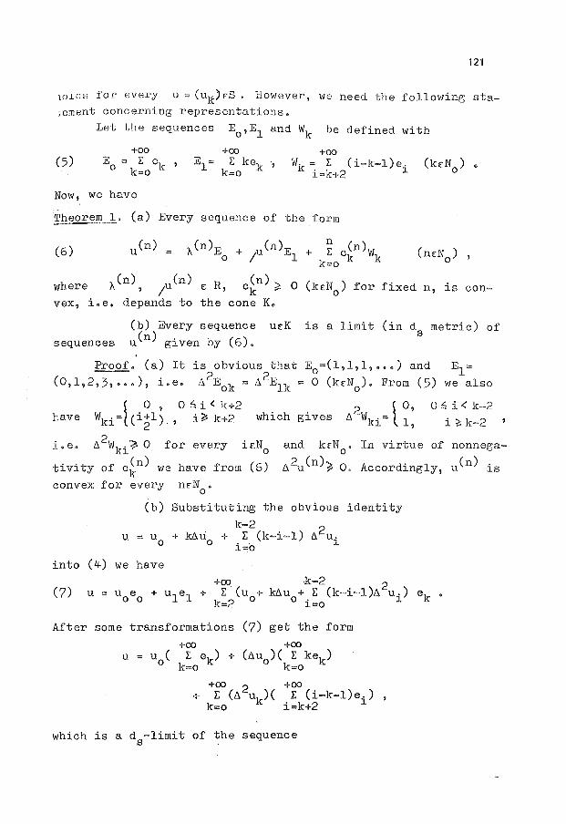
121
1o_tc.u:; for every u = (uk) cS . However, we need the followine; sta;ement concerning representations.
Let the sequences E0
,E1 and Wk be defined with
+OO +00 (5) E = l: e1 ,
0 k=O c Vl1 = l: (i-k-l)e. (k£N
0) •
c i=k+2 1.
Now, we have
Theorem L (a) Every sequence of the form
(6) (n)
u =
where "A (n), 1u(n) £ R, c~n) ~ 0 (kEN0
) f'or fixed n, is convex, i.e. depands to the cone K.
sequences (b) Every sequence UEK is a limit (in ds metric) of u(n) given by (6).
Proof. (a) It is obvious that E0=(l,l,l, ••• ) and E1 =
(0,1,2,3, ••• ), i.e. 6 2E0
k = 6 2E1k = 0 (kEN0). From (5) we also
have which gives 0 6 i < k-2
i ~ k-2 2 i.e. 6 V/ki~ 0 for every i£N
0
tivity of c~n) we have from (6)
and k£N0
• In virtue of nonnega-
62u(n)~ 0. Accordingly, u(n) is
convex for every
into (!.j.)
(b)
u = u 0
we have
ncN • 0
Substituting the obvious identity
k-2 + lffiu + l: (k-i-1) 6 2u.
0 i~o 1
(7) u +CO -k-2 2
u0
e0
+ u1e1 + l: (u + k6u + l: (k-i-1)6 u.) ek • k=2 ° 0 i=o 1
After some transformations (7) get the form
u = u ( 0
+00 +00 E ek) + (6u
0)( l: kek)
k=o k=o
+00 2 +00 + l: (6 u1 )( l: (i-k-l)ei),
k=O C i=k+2
which is a d -limit of the sequence s
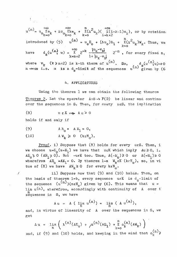
+00 + il u
0 l:kek +
k=o
introduced by (5) u(n)
have ( J +OO -k \Uk-Vk\
d5
(u n, u) E 2 2-n , for every fixed n, k=n+2 1+ \uk-v0
wher€ n~oo
vk (k l!:n+2) is k-th therm of u(n). So, d (u(n~u)~O i.e. u is a ds-limit of the sequences u(n) :iven by (6
4. APPLICATIONS
Using the theorem 1 we can obtain the following theorem
<rheorem 2. Let the operator A:S 4 F(D) be linear and continu' over the sequences in S. Then, for every ue:S, the implication
(8) u e:K ~ Au~ 0
holds if and only if
(9) A E = 0
A E1 = O,
(10) A wk ;:: 0 (k£N0
).
Proof. i) Suppose that (8) holds for every U£S. Then, i we ~boose u=E
0{u=E1) we have that ue:K which imply Au~O, i.
AE0 ~ 0 (AE1~ 0). But -ue-K too. Thus, A(-E0 )~ 0 or A(-E1 );:: 0 wherefrom AE
0 =AE1= 0. B,y theorem 1-a Wke:K (krN
0), so, in vi
tue of (8) we have AWk~ 0 for every k~N0 •
1 ii) Suppose now that (9) and (10) holds. Then, on the basis of theorem 1-b, every sequence ue-K is ds-limit of the sequence (u(n))(ne:N
0) given by (6). This means that u =
lim u (n), wherefrom, accordingly with continuity of A over t. n .
sequences ~n S, we have
Au A(limu(n)) n
and, in virtue of linearity of A get
lim(Au(n)), n
over the sequences in S, we
Au lim ( ~(n)(AE) + u(n)(AE) n o I 1 +k~oc~n)(AWk) J
and, if (9) and (10) holds, and keeping in the mind that c~n)~

~e .unaly obtain A u~O
~emark l. It is easy to see that our theorem 2 generalizes the ~esul t of theorem 4 in [ l] • In this case an operator A have
the .form -of triangular matrix.
Remark 2. The representation (6) is a discrete analogue of the relation (6) in [ 2 J • 'l'he sequences Wk we can call a discrete splines.
REFERENCES
1. MITRINOVIC D.S., LACKOVIC I.BqSTANKOVIC M.S.: Addenda to the monograph "Analytic Inequalities" II. On some convex sequences connected with N.Ozeki's result. Univ. Beograd. Publ. El~ktrotehn. Fak. Ser. Mat. Fiz. No 634- No 677 (1969),3-24
2. VASIC P.M., LACKOVIC I.E.: Notes on convex functions II: On continuous linear operators defined on a cone of convex functions. ibid. No 602 - No 633 (1978), 53-59.
I
I
I
I
I
I
I I
I
I
I
I
I I
I
I
I
I
I
I
I
I

Numerical Methods and
Approximation Theory
Nis, September 26-28, 1984
APPROXIMATION OF CONVEX FUNCTIONS BY FIRST DEGREE SPLINES
Ljubisa M. Koci6
ABSTRACT:
A method for ~pproximation of functions convex on a finite interval by picewise affine function is developed. For the segments of approximating function we used the support affine function f in prescribed points, and its graph lies not up then the graph of f •
APROKSH'IACIJA KONVEKSNIH FUNKCIJA SPLAJNOVIMA PRVOG STEPENA. U radu je razvijen metod aproksimacije konveksne funkcije, ueo po deo afinom funkcijom. Segmenti aproksimirajuce funkcije su potporne afine funkcije aproksimirane funkcije f u zadatim tackama, a njen g~afik lezi ne iznad grafika funkcije f •
1. INTRODUCTION
The problem of approximation of one variable function by
first degree splines (picewise affine functions, polygonal lines)
is minutely studied from many autors,and for classes CCa,bJ and
c2 ca,bJ , as well as the interpolated classes H~ and WHw,
see, for example. [ l J and [' 3 J • A lot of results are oriented t<
applications on computers [7J. In all appearance, this kind of
approximation is especially important for convex functions. Erly
results was obtained by K. TODA ( 6 J and T. POPOVICIU [ 4 J.
They were shown the following theorem:
Theorem 1. The first degree spline function
(l) (Sf)(x)=pX+q+ n x E [a, b] , n EN ,
125
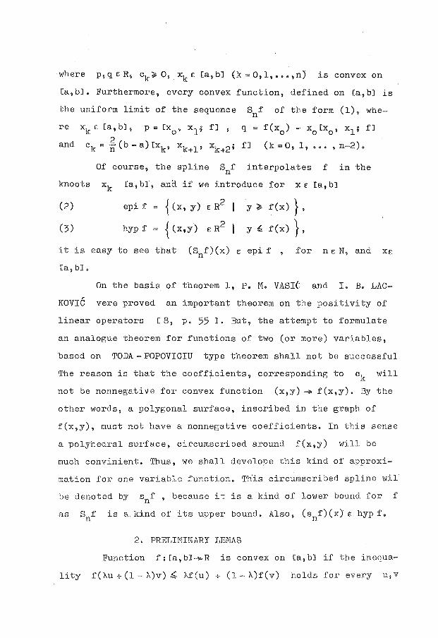
where p, q_ £ R, ck ~ 0, xk £ [a, bJ (k = 0, l, ••• , n) is convex on
[a,bJ. Furthermore, every convex function, defined on (a,bl is
the uniform limit of the seq_uence Snf of the form (1), whe-
re
and
Of course, the spline Snf interpolates f in the
knoots xk (a, bJ, ana if we introduce for XI: [a, bJ
(2) epif { (x, y) £ R2 y ~ f(x) } ' (3) hyp f { (x,y) 2 y ~ f(x) } ' = £R
it is easy to see that (Snf) (x) £ epi f ' for n e: N, and xe-
[a, bJ.
On the basis of theorem 1, P. M. VASIC and I. B. LAC
KOVIC vere proved an important theorem on the positivity of
linear operators [8, p. 55 J. But, the attempt to formulate
an analogue theorem for functions of two (or more) variables,
'based on TODA - POPOVICIU type theorem shall not be successful
'I'he reason is that the coefficients, corresponding to ck will
not be nonnegative for convex function (x,y)-+ f(x,y). By the
other words, a polygonal surface, inscribed in the graph of
f(x,y), must not have a nonnegative coefficients. In this sense
a polyhedral surface, circumscribed around f(x,y) will be
much convinient. Thus, we shall develope this kind of approxi
mation for one variable function. Ttiis circumscribed spline wil
be denoted by snf , because it is a kind of lower bound for f
as Snf is a. kind of its upper bound. Also, (snf) (x) e: hyp f.
2. PRELIMINARY LEr1AS
Function f: Ca,bJ~R is convex on (a,b] if the inequa-
lity f('Au + (1- 'A)v) ~ M(u) + (1- 'A)f(v) holds for every u, v

121
ta, oJ and A. E: (0 9 l) • The function f is called strictly con
:lX if above inequality is strict. Let K(a, bJ and K+(a, bJ
:lnote the cones of convex and strictly convex functions on
:a, bJ , continuous from the left (right) at the edge point a
:b). The function x- p(t,x) is called support function of con
rex function f if the following conditions are fulfiled :
f(x) ~ p(t,x), x e:. [a,bJ , x ,lt and f(t) = p(t,t).
'or strictly convex functions the following lemma takes place
see for ex. [ 5l):
,emma l. Let f: [a, bJ -+ R be strictly convex on [a, bJ, and let
'(x) be the right derivative of f in x. Then +
a) f' is increasing function on [a,bJ , +
b) for every a ~ u < v ~ b holds
f'(u) < f(v)- f(u) < f'(v). + v - u +
Let f £ K+ [a, bJ , and x 1 < x 2 ( ••• < xn be a set of knoots
from (a,b). The first order spline, circumscribed around the
graph of f is given by
(4-) (s f)(x) = sup { p(xi'x) } , x e: [a, bJ , n l~i~n .
where p(xi ,x) is affine sup,port function of f in the uoint x1 :
(5) P(x.,x) = f(x.) + f'(x.)(x-x.) • D l l + l l
So we have
Lemma 2. a) sn f interpolates f in the knoots xl' • •. 'xn'
b) sn f is convex on [a, bJ.
Proof. a) Let 1~ k~ n be a fixed number. Then, sup {p(xi ,xk)} H:Hn
p(xk,xk) = f(xk) which is an interrelate prOlJerty.
b) As every function x r- p(xi'x) (i = 1, 2, •• q n) is
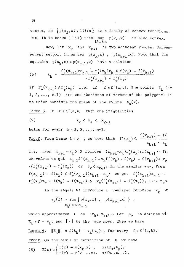
28
convex, so ~ p(xi, x) I H.Hn} is a family of convex functions.
3ut, it is known ( [ 5 J) that sup p(xi,x) lH~n
is also convex.
Now, let xk and xk+l be two adjacent knoots. Corres-
podent support lines are p(xk,x) , p(xk+l'x). Note that the
equation p(xk,x) = p(xk+l ,x) have a solution
(6)
l, 2, ••• , n-l) are the abscisses of vertex of the polygonal li
ne which consists the graph of the spline sn(x).
Lemma 3· If f e: K+ [a, bJ then the inequalities
holds for every k = l, 2, ••• , n-1.
) - f( Proof. From lemma 1- b) , we have that f:(xk) <.
xk+l - xk
i.e. from xk+l -xk> 0 follows (xk+l-xk)f:(xk)<f(xk+l) -f(
wherefrom we get xk+lf:(xk+l) -xkf:(xk) +f(xk)- f(xk+l)< xk
·(f:(xk+l) - f:(xk)) or tk< xk+l" In the similar way, from
f(xk+l) - f(xk) < f:(xk+l)(xk+l -xk) we get f:(xk+l)xk+l -
f:(xk)xk + f(xk) - f(xk+l) > xkcr:cxk+l) - f:(xk)), i.e. tk>
In the seqel, we introduce a v-shaped function
vk(x) = sup/ p(xk,x) , p(xk+l'x) } ,
xk~x :s; xk+l
w:
which approximates f on [xk' xk+l J. Let ~ be defined wi ~
Ek = f - vk' and 11·11 be the sup norm. Then we have
Lemma 4. 11~11 = f(tk) - vk(tk) , for every f e: K+ (a, bJ.
Proof. On the basis of definition of E we have
(8) E(x) "' ( f(x) - p(xk 1 x) , xe: [xk' tk), i f(x) - n(x, •• x). xr(t,_.x,_.,J.
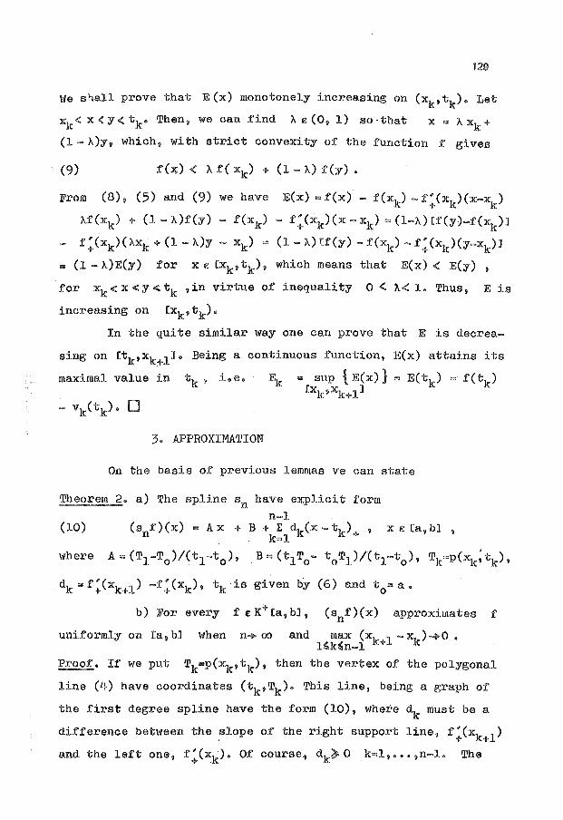
129
We shall prove that E(x) monotonely increasing on (xk,tk). Let
xk<x<y<tk. Then, we can f'ind "Ae:(O, 1) so·that x"' "Axk+
(1- "A)y, which, with strict convexity of the function f' gives
(9)
From (8), (5) and (9) we have E(x) = f(x) - f(xk) - f': (xk)(:x:-xk)
"Af'(xk) + (1-"A)f(y)- f'(xk)- f'~(xk)(x-xk) =(1-1\)Cf(y)-f(xk)J
- f ~ (xk)( "Axk + (1 - "A)y - xk) = (1- "A) tf(y) - f(xk) - f~ (xk)(y-xk)J
= (1- "A)E(y) f'or x E [xk,tk)' which means that E(x) < E(y) ,
for xk < x < y < tk , in virtue of' inequality 0 <. "< 1. Thus, E is
increasing on (xk,tk).
In the quite similar wa:y one can prove that E is decrea
sing on [tk,xk+lJ. Being a continuous function, E(x) attains its
maximal value in tk , i.e. ~ = sup { E(x)} = E(tk) = f(tk) [xk,xk+ll
3. APPROXIMATION
On the basis of previous lemmas ve can state
Theorem 2. a) The spline sn have explicit f'orm
n-1 (10) (snf)(x) =Ax + B +I: dk(x-tk)+ , x e: (a 9 b] ,
. k=l
where A=(T1-T0)/(t1-t
0), B=(t1T
0- t
0T1 )/(t1-t
0), Tk=p(xk;tk),
dk = f~(xk+l) -f~(xk)' tk is given by (6) and t0
= a.
b) For every f e: K+ (a, bJ, ( snf') (x) approximates f
uniformly on [a,bJ when n+oo
~· If we put Tk=p(xk,tk)' then the vertex of the polygonal
line (4) have coordinates (tk,Tk). This line, being a graph of
the first degree spline have the form (10), where dk must be a
difference between the slope of' the right support line, f~(xk+l)
and the left one, f'~(xk). Of course 1 dk~O k=l, ••• ,n-1. The

proof of b) follows from lemma 4. Namely, for xe:[xk,xk+lJ' we
have jf(x)- vk(x)l ~ E(tk) = f(tk) -f(xk) -f~(xk)(tk-xk)' and
i:f we put h=xk+l-xk, then lr(tk) -f'(xk)r~ w(f,h), and also
tk- xk < h, wherefrom lf(x) - vk(x) I< w(f ,h) + h -+0, and according
ly, f'(x) - sn (x) -0, WhE:Jn n-+ oo and m~x(xk+l- ~)-o •
Sofar we deal only with strictly convex functions. What we have pointed out it is that no difficulties when we pass to convex functions. Namely, these subintervals of (a,bJ on which f is affine, must be excluded, and remainded graph will be a strictly convex function. Now, we under-line that the form of the spl ne does not new. There is no difference, ·in formal sense, betwee
Snf and snf. However, we have snf ~ f ~ Snf on (a, b], and n e:
.!!'rom this reason, we call S f an upper spline and s f a low n n spline of the convex function f. There is, also, a middle spl ne, have been studying by r1. GAVRILOVIC in [ 2 J and provid the mini-max approximation. The spline Snf exists for every tinuous function. But, the middle and the lower spline do exis only for convex functions.
REFERENCES
1. ALBERG J.H., NILSON E.N., WALSrt'J.L .• : The theory of splines and their applications (in russian, by complements of S.B. Steckin and Yu.N. Subotin), Moscow 1972.
2. GAVRILOVIC M. 1\1.: Optimal approximation of convex curves by functions which are picewise linear. J. Math. Anal. Appl. 5 (1975), 260-282. -
3· MALOZEMOV V.N.: Ob otklonenii lomanyh. Vestnik Leningrad. U niv. 21 (1966), 150-153·
4. POPOVICIU, T.: Sur certaines inegalites qui caracterisent l fonctions convexes. A. Sti. Univ. "Al. I. Cusa" Iasi Sect. Math. (N.S.)-11 B (1965), 155-146. '
5· ROBERTS A.W., VARBERG D.E.: Convex functions. New York- Lo don 1973.
6. TODA K.: A method of approximation of convex functions. TOb ku !"'ath. J. 42 (1936), 311-317.
7• PAVLIDIS T.: Polygonal approximation by Newton's method. IEEE Trans. Computers. C-26 (1977), 800-80).
8. VASIC P.M., LACKOVIC LB.: Notes on convex functions II: Oil continuous linear operators defined on a cone of convex fu~ ctions. Univ. Beograd. Publ. Elektrotehn. Fak. Ser. ~1at. F1 No 602- No 633 (1978), 53- 59.
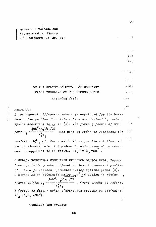
Numerical Methods and
Approximation Theory
Nis, September 26-28, 1984
ON ~HE SPLINE SOLUTIONS 0~ BOUNDARY
VALUE PROBLEMS OF THE SECOND ORDER
Katarina Surla
ABSTRACT:
A tridiagonal difference scheme is developed for tb.e boun
dary value pPobZem (1). This scheme was derived by cubic
spline aaaording toIl 'in [2]. The fitting factor of the 2 ;-
2sh {h.Vq .. /2) form a, = · · 2 ~ ~ was used in order to e Ziminate the
~ h igi
condition h~q. <6. Ex>ror estimations- for the solution and ~ ~-
it& derivatives are also given. In some oases these esti-
mations appeared to be optimal (Sa =0 ,h0
=Mh2).
0 SPLAJN RE~ENJIMA KQNTURNIR PROBLEMA· DRUGOG REDA. Posma
tPana je tx>idiagonaZna difex>encma 8ema za konturni problem
(1}. Bema je izvedena primenom kubnog spZajna prema [3]. u nameri da se eZimini8e uslov h.q~<6 uveden je fiting
---~ ~-2sh2
{h .V q1
/2) faktor obZika a
1 = 2 ~ • Ocene greske za Pesenje
hiqi i izvode su date, U nekim sZuoajevima proaene su optimalne
{[) =O,h. =Mh2). a o
Consider the problem
131
; i;
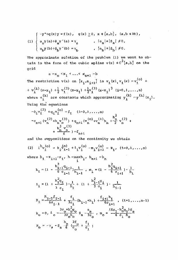
( 1) l-y"+q(x)y =f(x),
atay(a)+eay'(a) =ya
ctby<b>+eby'<b> =rb
g(x) _::o, x e [a,b], (a,b eiR),
, lctal+leal ~o,
, I ctb I + I Bb I ~ 0 •
The approximate solution of the problem (1) we wont to ob
tain in the .form of the cubic spline v(x) ec 2 [a,b} on the
grid
a =x0
< x 1 < ••• :< x·n+1 =b
The restriction v(x) on [x1
,xi+1
] is vi(x),vi(x) =v!o) +
. ( l_) 1 ( 2) 1 ( 3) . 3 -+ 'l.l"i (:x-x1> +2 v:i (x-x1) +2vi (x-x1 ) (i-0,1, ••• ,n)
(k) (k) (k) where vi are constants which approximating y i = y (xi) •
. ' Using th.e equations . (2) (o)
-q·ivi +qivi =fi (i=O,l, ••• ,n)
and the suppositions on the continuity we obtain
(2) Lhvio) = k:i:~~: 1 +~ivio) -mivi~i = Ri, (i=0,1, ••• ,n)

c = (1 -n
c 3abhn + 6f3b
abhn + 36b '
m =0 n
(k) The consta,nts v 1 , k=1, 2, 3 we obtain from the relations
a v(o) + 6 v< 1 > = Y~ a 0 a 0 a
2 h2 2 2fi-1 fi hi-lqi
f3 =1 + i-1qi-l hi-1
ai = 1 - 6 , 3 I s. =--- (--- +-) q i 0 i-l J. 2 0 i-1 °i i
h v(o) v(o) (1) (1) + n-1 ( qn :n +
qn-1 n-1 ) vn v:n-1 r --- , n 2 o1 qn-1
hn-1 f:n-1 f ( :n
rn -2- --+ 0n-1 0 n
-o (v( 2)+h v(J))+q ( v(o) + v( 1 )h +h2v( 2 )/2 + n+1 n n n n+1 n n n n n
+ h 3v(J) /6) = f n n n+l
Similar to [2] it can be shown that zlk) =ylk) -vlk) sa
tisfy the equations
133
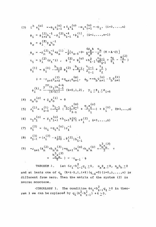
( 3)
(4)
( 5)
(6)
01
( 8)
{9)
h {o) (o) {o) (o) _ (. _ ) L z. =-k_.z,
1 +t.z. -m.z.+1 --1)J., ~-O, .•• ,n
L ~ ~- 1 1 ~ 1 1
(o) q. z ~o) Z
(l)_ z(l) +hi-1. (qi-lzi-1 + 1 :1. ) + A-.(1)~ - · 1 -2- 'I' • (i=1, .•• ,n)
i 1- a i- 1 ai 1
i=1, ••• ,n)
- ( z ( 2 ) +h z ( 3 ) ) +q ( z { 0 ) +h z ( 1 ) an+~ n n n n+l n n n
h3z (3)
+ ...Jl...1L.. ) 6
+
THEOREM 1. 2 Let 6a1-hi-lqi .:_o, aa8a 2_0, ab8b .:_0
and at leats one of
different from zero.
nverse monotone.
qk (k=i-l,i,i+l) (q_ 1=0) (i=O,l, ••• ,n) is
Then the matrix of the system (2) is
-COROLLARY 1. The condition 6cri-h~ 1q. >0 in theo
rem 1 we can be replaced by q. (h~-h~ 1
) +6:1.~0.1
-1 ~ 1-

THEOREM 2. Let the boundary value problem (1) has 4
a unique solution y (x) e C [a,b]. Let conditions of theorem 1
are fulfilled.
Then for S ~0 the following holds a
izt)l 2_Mh2
(k=O,ll2)1 izl3
)!2_Mh
and for sa= 0
I z~k) I <Mh (k=O,l,2) 1 I z~ 3 ) I <M , where !4 denotes 1 - 1 -
different constants, independent on h.
(11)
(12)
Proof.
(i=l 1 ••• ,n)
b. 0
so<sl-~) --,-h-- - aa >Mh
0
From (10), (11) and (12) we obtain that II A-1 1!.::_ rna~/':,.- .::_Mh-:
A is matrix of the system {2) • i 1
Since jai-11 .::_Mh2
we have !lJ!il =O(h3
} and then
lz{o) I .::_i!A-il!llJ!il 2_Mh2
The estimates for ] z ~k) I (k=1, 2, 3) we obtain from relations 1
(4) -{9).
THEOREM 3.
ons of the theorem 1
Jz~o) I <Mh3 ; 1 -,-
Let hi =h=cons~, Ba =sb=O and the conditi
are fulfllled. Then
Jzik)j .::_Mh2
; jz_in I .::_Mh 1 (k=1,2)
- -1 Proof. A simple calculation shows that A >h B,
135
where A is matrix determined by {3) for i=l 2 ••• ,n, ~nd z~0 )=0, B = {bi.} (L, j=l 1 ••• ,n~ is tridiagonal matrix with b .. =2,
J 11
bi 11 =-1, (i=2, ... ,n), b .=-1 (i=1, ... 1 n-1). -I i+li<J.
The solution of the system

I I i (n+l-i) Bu =w, w=max 1/Ji h has the form ui = 2 w • Since
I z l 0 ) I _::. u i we h! ve I z ~ 0 ) I _::. u 1 = 0 ( h 3
) , I z ~ 0 ) I _::. un = 0 ( h 3
) •
Then form (3) for i=2 we obtain z~0)=0(h 3 ) and then by in-
1 (o) I 3 duction we can conclude that zi =O(h) (i=2, ••. ,n). The
estimates for derivatives we get from (5)-(9).
THEOREM 3. Let Ba=O and h =Mh2
Then 0 •
lz~k) ~ <Mh4-k (k=O,l,2,3).
~ -
Proof. See l4].
REFERENCES
1. Doolan,E.P., Miller J.J.H.,Sehfiders W.H.A., Uniform nume
riaa~ methods for prob~ems with Initia~ and Boundary
Layers. BOOLE Press, Dub~ine, 1980.
2. Il~in V.P., 0 sp~aynovyh resenijah obyknovenyh differen
aia~ 'nyh uravnenij. ~urnaL vycisZ. mat. i mat. fiz.,. No
3, (1978), 621-627.
3. Surla K., Kulpinski M., 0 splajn resenjimq obionih dife
renaija~nih jednaaina, Zbornik radova, V Znanstveni skup
Proraaunavanje i projektovanje pomodu raauna~a. Stubia
ke TopZiae, 1983, 137-141.
4. Surla K., Accuracy indrease for some sp~ine so~utions of
two-point boundary va~ue prob~ems, Rev. of Research Faa.
of Sci. Univ. of Novi Sad, Vo~ume 13 (1983) (in press).
5. Jain M.K., Aziz T., Numeriaa~ so~ution of stiff and con
vection-diffusion equations using adaptive sp~ine func
tion approximation. Appl. Math. Modelling, Vol. 7~ Feb
ruary ( 1 9 8 3) • 5 7-6 2.
6. Zavjalov, Ju.s., Kvasov B.I., Mirolni~enko Z.L., Metody
splajn funkaii, Moskva 1980.

Numerical. Methods and
Approximation Theory
Nis, September 26-28, 1984
MESH CONSTRUCTION FOR NUMERICAL SOLUTION
OF A TYPE OF SINGULAR PERTURBATION PROBLE~qS
Relja Vulanovic
,BSTRACT:
~e singular perturbation problem (1) is considered. It is ·oZved numerically by classical difference schemes on a nonniform mesh. The discretization mesh is construced in a pecial way. which gives linear convergence uniform in small •erturbation parameter.
KONSTRUKCIJA P.1REZE ZA NUMERICKO RESAVANJE
JEDNOG TIPA SINGULARNIH PERTURBACIONIH PROBLEP.A
posmatra se singularni perturbacioni problem (1) koji se re-8ava numerioki pomodu klasianih diferencnih .8ema na neekvidistantnoj mrezi. Mreza diskretizacije se konstrui8e na specijalan naain. tako da se dobija linearna konvergenoija uniformna po malom perturbaoionom parametru.
1. INTRODUCTION
We consider the two point boundary value problem
(1a) Leu:= e 2u" +xb(x)u; -c(x)u =f(x), x €I = [0,1]
(lb) u(O) =U0
, u(l) =U1
,
with basic asumptions
2 b,c,f €C (I)
b(x) > 2(3 >0, c(x) ?_Y. >0, 2b(O) <c(O) ,
0 < £ 2 €0 •
This problem was solved in [2] by a sp~cial method
which gives linear convergence uniform in small perturba
tion parameter e:. Our method seems to be somewhat simpler.
It is based on the idea of Bahvalov, [1], that was genera-
137
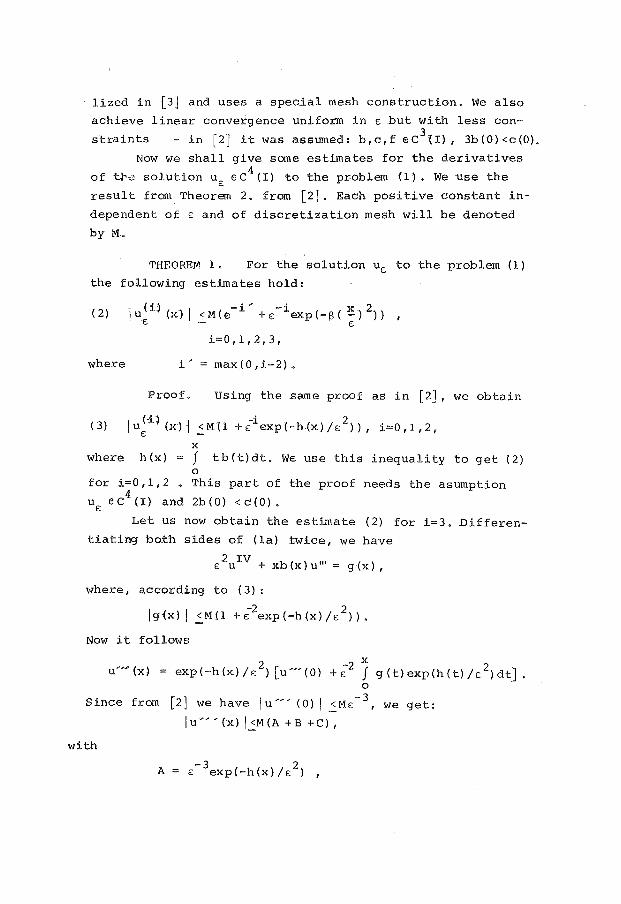
lized in [3] and uses a special mesh construction. We also
achieve linear convergence uniform in £ but with less con
straints - in [2] it was assumed: b,c,f ec 3:{I), 3b{O)<c(O).
Now we shall give some estimates for the derivatives
of tp~ solution u£ ec4 {I) to the problem {1). We use the
result from Theorem 2. from {2]. Each positive constant in
dependent of £ and of discretization mesh will be denoted
by M.
THEOREM 1. For the solution u£ to the problem (1)
the following estimates hold:
( 2) (i) -i' -i X 2 lu (x) I <M(e +s exp(-13( -) )) ,
£ - £
i=0,1,2,3,
where max (0, i-2).
Proof. Using the same proof as in [2], we obtain
( 3) I ( i~ 1 -i . 2 u (x} <M{l +s exp(-h(x)/£ )) , i=0,1,2, £ -
X
where h(x} f tb(t)dt. We use this inequality to get (2) 0
for i=0,1,2 This part of the proof needs the asumption 4
u£ ec (I) and 2b(O) <c(O).
Let us now obtain the estimate (2) for i=3. Differen
tiating both sides of ( la) twice, we have
s 2uiV + xb(x)u'" = g(x),
where, according to (3):
-2 2 lg{x1j _:M{l +s exp(-h(x)/£ )).
Now it follows
2 ~ X 2 u'"(x) = exp(-h(x)/£ >[u'N(O) +s J g(t)exp(h(t)/£ )dt].
0
Since from [2] we have I u '" (0) I ..:::_Ms - 3 , we get:
I u '' - (X) I..:::_M (A + B + c ) J
with
A -3 2
£ exp(-h(x)/£ ) ,
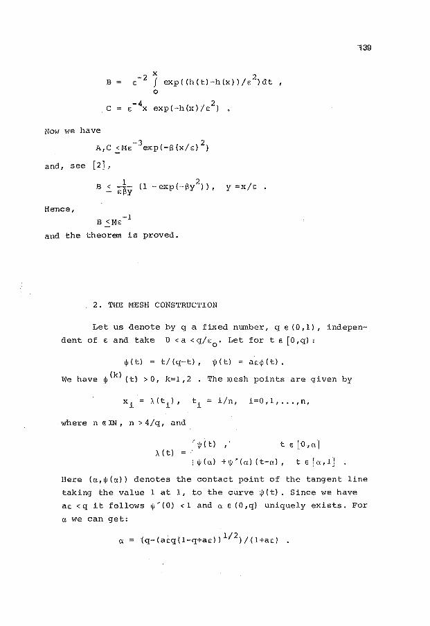
139
B 2 X 2
£- f exp((h(t)-h(x))/£ )dt 0
C £- 4x exp(-h(x)1£ 2) •
Now we have -3 2
A,C ~l-1£ exp(-8 (x/£) )
and, see [2],
1 2 B < £BY (1 - exp(-(3y ) ) , y =x/£ •
Hence, B <ME - 1
and the theorem is proved.
2. THE MESH CONSTRUCTION
Let us denote by q a fixed number, q e (0,1), indepen
dent of £ and take 0 <a <q/£0
• Let for t e [O,q):
<j>(t) = t/(q-t), l)J(t) = a£<j>(t).
We have <j>(k) (t} >0, k=1,2 . The mesh points are given by
where n e lN, n > 4/q, and
A (t) = ·· t e !D , o: J
Here (a 1 l)J(a)) denotes the contact point of the tangent line
taking the value 1 at 1, to the curve l)J(t). Since we have
a£ <q it follows l)J'(O) <1 and a e (O,q) uniquely exists. For
a we can get:
a = 1/2 (q-(a£q(1-q+a£)) )/(l+a£) .
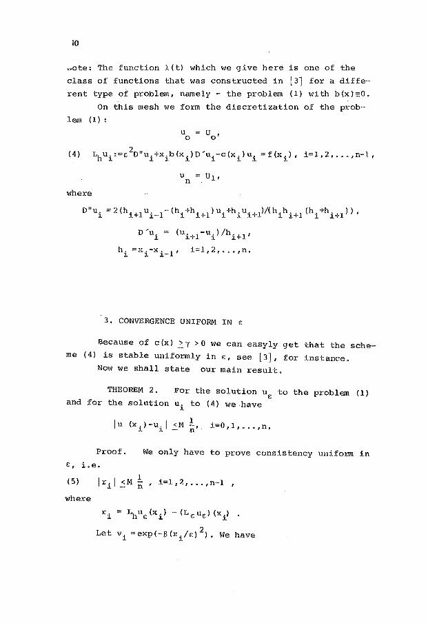
10
.. ote: The function A{ t) which we give here is one of the
class of functions that was constructed in [31 for a diffe
rent type of problem, namely - the preblem (1) with b(x}=O.
On this mesh we form the discretization of the prob
lem (1):
where
D'ui = (ui+1-ui)/hi+l'
hi =xi-xi_1 , i=l,2, ••. ,n.
3. CONVERGENCE UNIFORM IN e:
Because of c(x) ~Y >0 we can easyly get that the sche
me (4) is stable uniformly in e:, see [3], for instance.
Now we shall state our main result.
THEOREM 2. For the solution u£ to the problem (1) and for the solution ui to (4) we have
lu (x.)-u.l <M Ln'- i=O,l, •.• ,n. l. l. -
Probf. We only have to prove consistency uniform in e:, i.e.
(5) lril <M ~, i=1,2, ... ,n-l,
where
ri = Lhue:(xi) -(Le:ue;)(xi~
Let vi =exp(-{3(xi/e:) 2). We have
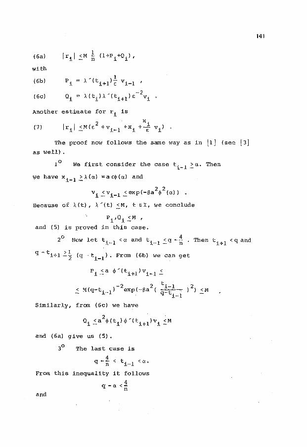
(6a) lril <M 1
(l+Pi+Qi), n
with
(6b) P. ;.. '(ti+l)i vi-1 , ~
(6c) Qi ;.. (ti);.. '(ti+l) £ -2
vi
Another estimate for ri is
(7) 2 xi
lril :s_M(£ +vi-1 +xi+£ vi)
The proof now follo~Ts the same way as in [1] (see [3] as well).
1° We first consider the case ti-l ~a. Then
we have xi-l ~)..(a) =a£(j>(a) and
2 2 vi :s_vi-l :s_exp(-Sa <P (a))
Because of )..(t), ).. '(t) :s_M, t ei, we conclude
Pi,Qi :s_M '
and (5) is proved in this case.
2° Now let ti-l <a and ti_ 1 :s_q-·~
q-ti+l>l (q-t. 1). From (6b) wecanget -2 1.-
Pi :s_a <j>'(ti+l)vi-1 :5.
Then ti+l < q and
-2 2 ti-l )2) < M(q-ti-l) exp(-8a ( q-ti-l <M
Similarly, from (6c) we have
Q. <a2
<j>(ti)<j>'(t.+1 )v. <M ~- ~ ~-
and (6a) give us (5).
3° The last case is
4 q -:n < ti-l <a.
From this inequality it follows
4 q- a <n:
and
141

(8)
because
q - (J. > ~-(-1-gl:g £
l+q
Now xi_ 1 ·> ae:cp (q -~ } , (notice q - * > 0), and we get
(9) < M l vi-1 n
Similarly:
( 1 0) Xi v . < MV;- < M l e: J.- J. n
For xi we have
xi /.. (ti) .::_;..(ti-l) +M * and
/..(ti-1) </..(a) <M/£,
hence, using (8) we get
(11) X. <M .!_ J. n
Now from (7-11) it follows (5) and the theorem is. proved.
REFERENCES
1. Bahvalov,N.S.: K optimizacii metodov resenija kraevyh
zadac pri naticii pogranicnogo stoja, z. vycist. mat. i
mat fiz., T9, No 4 (1969), 841-859.
2. Lisejkin,V.D.: 0 cistennom resenii obyknovennogo diffe
renciat 'nogo uravnenia vtorogo porjadka s matym parame
trom pri starsej proizvodno~6istennye metody meh.splosnoj sredy, T13, No J (1982), 71-80.
3. Vulanovic,R.: Numericko resavanje konturnog problema
drugog reda sa malim parametrom, magistarski rad, Novi
Sad, 1983.
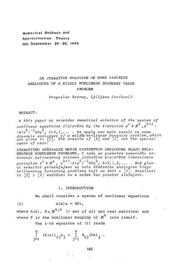
Numerical Methods and
Approximation Theory
Nis, September 26-.28, 1984
AN ITERATIVE SOLUTION OF SOME DISCRETE
ANALOGUES OF A MILDLY NONLINEAR BOUNDARY VALUE
PROBLEM
Dragoslav Herceg, Ljiljana Cvetkovid
.BSTRACT:
n this paper we consider numerical solution of the system of
,.on linear equations A (x)x=BFx by the iteration x 0 e IRn ,xk+1 = k -1 k . =A (x ) BFx , k=0,1, ... . We apply our ma1-n result on some
discrete analogues of a mikiJu nonlineqr boundary 'problem, which are given in [1]. The results of [2] and· [3] are the special cases of ours.
ITERATIVNO RESAVANJE NEKIH DISKRETNIH ANALOGONA BLAGO NELINEARNIH KONTURNIH PROBLEMA. U radu se posmatra numericko resavanje nelinearnog sistema jednaaina A(x)x=BFx iterativnim
o n k+1 k -1 k v postupkom X elR, x =A(x) BFx, k=0,1,2, .... Nas glav-ni rezultat primenjujemo na neke diskretne analo~one blago nelinearnog konturnog problema koji su dati u [1J. Rezultati iz [2] i [3] Eiadrzani su u nasem kao posebni sluaajevi.
l, ;I:NT:RODUCT!ON
We shall consider a system of nonlinear equations
(I) A(x)x = BFx,
\'There A (x) , Be JRn, n (= set of all rum real matrices) and
where F is the nonlinear mapping of JRn into itself.
The i-th equation of (I) reads
n /,
j=l (A(x)) .. x.
~J J
n
/. BiJ' (Fx) J' • j=l
143
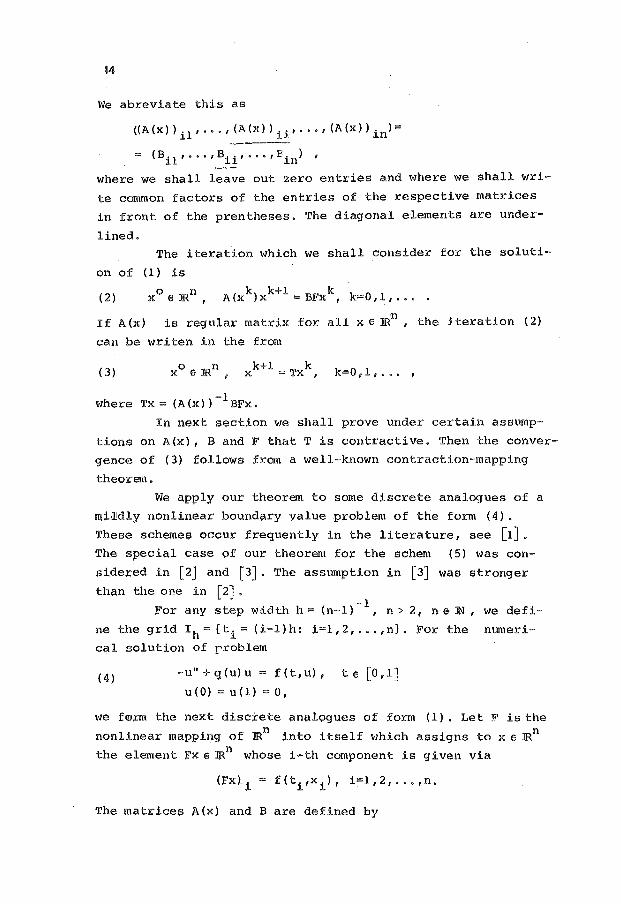
i4
We abreviate this as
((A(x)) . 1 , ... , (A(x)) .. 1 ••• , (A(x)) in)= l. J.l.
= (Bil'''' 18ii'''"'Ein) '
where we shall leave out zero entries and where we shall wri
te common factors of the entries of the respective matrices
in front of the prentheses. The diagonal elements are under
lined. The iteration which we shall consider for the soluti-·
on of (1) is
(2) o n
X € JR 1
If A(x) is regular matrix for all x e IRn, the Jteration (2)
can be \'lri ten in the from
~1here Tx = (A (x)) - 1 BFx.
In next section we shall prove under certain assump-·
tions on A(x), Band F that Tis contractive. Then the conver
gence of (3) follows from a well-known contraction-mapping
theorem.
We apply our theorem to some discrete analogues of a
miilldly nonlinear boundary value .problem of the form (4).
These schemes occur frequently in the literature, see [1].
The special case of our theorem for the schem (5) was con
sidered in [2] and [3] . The assumption in [3] was stronger
than the one in [2] . -1
For any step wd.dth h = (n-1) , n > 2 1 n e lN 1 we defi-
ne the grid Ih = {ti = ( i-1) h: i=1, 2, •• , , n}. For the numeri
cal solution of rroblem
(4) -u"+q(u)u = f(t,u), te [0,1]
u(O) =u(l) =0,
we f@rm the next discrete analogues of form (1). Let F is the
nonlinear mapping of IRn into itself \'Thich assigns to x e IRn
the element FX e JRn whose i-th component is given via
(Fx)i
The matrices A(x) and B are defined by

[5) -2 2 h (-1 12+h q{x.) 1-1)
___ _::_....!._ ~1) for i=2 13 1 .•. 1n-1 1 (second
)rder approximation) 1
h- 2 2 (6) T:f (1~-16 1 30+12h q(xi) 1 -1611)={~) 1 for i=3 1 4 1 ••• ,n-2 1
(fourth order approximation) 1 and second order approximation
tor i=2,n-1 as in (5),
(7) h-2 ~
180 (-2,27,-270,490+180h~q(xi) 1 -270 1 27 1 -2)=(~) for i=;4 1
5 1 ••• 1 n-3 1 (sixth crder approximation) 1 and fourth order ap
proximation for i=3 1n-2 as in (6) 1
and a fourth order unsymmetric approximation
h - 2 2 T:f (-10,15+12h q(xi) ,4,-14 16 1-1)=(_!) for i=2,
h- 2 2 l2 (-1 16,-14,4,15+12h q(xi) ,-10)=(_!) for i=n-1.
In (5), (6) and (7) we have (1)=(_Q) for i=1,n.
145
T n The solution x = [x
1,x 2 , •.. ,xn] e JR of (1) is the nu-
merical solution of the boundary value problem (4), i.e.
xi:tu(ti), i=1,2, ... ,n.
THE CONVERGENCE ANALYSIS
Theorem. Let A (x) "' [a .. (x) J e JRn 1 n is inverse-mono. ~J tone matrix for all x € ]Rn and let BF is Frechet-·differentJo.ble
in JRn. Suppose that
1*en the equation (1} has a unique solution and the sequence 0 1 2
x ,x ,x , ... , generated by (3) converges to this solution.
Proof. We shall prove that IJ T '(x) Jl co < 1, where
T'(x) is Frechet derivative of Tx=A(x)-1
BFx. Let C(x) = [c .. {x)] '"'A{x)-
1 and let y e JRn. From [3] we have
~] .
T' (y) = (C (x) BFy) '(y) + C (y) (BF) '(y).
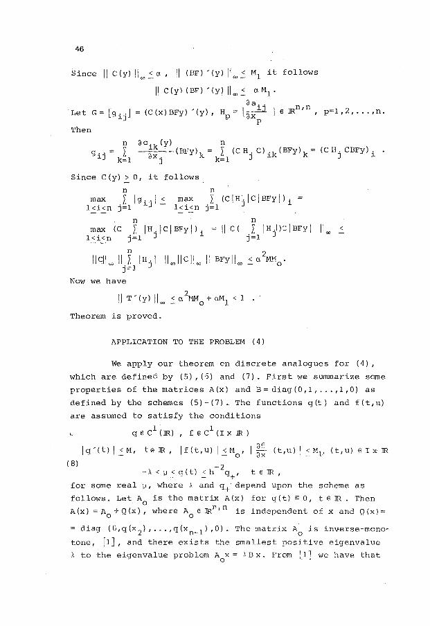
46
Since II C(y) II""_: a:, !! (BF) '(y) lloo.2. ~1 1 it follows
II c ( y) ( BF) ' ( y) II 00 ..:. 0: M 1 .
a a .. (C(x)BFy) '(y), H = la·xD _16 JRn,n, p=1,2, ... ,n.
p p
Then
n a cik (y) n _ g {J' = l ---;;-x---(BFy) k = l (C HJ. C) ik (BFy) k- (C HJ. CBFy) i .
.._ k=1 ° j k=1
Since C(y)..::.o, it follows
n n max l I g .. I < max /, ( C I H j I C I BFy I ) i =
1_:i_:n j=1 ~J - 1_:i_:n j=1 _ _
n n max (C /, jH.jC~BFylli =II C( /, IH.[):jBFyl lloo <
1<i<n j=l J j=1 J
n
llcJioo lljL1
1Hj I lloollclloo II BFylloo 2
< 0: ~1 • 0
Now we have
2 II T'(y) llco .2. o: ~1Mo + o:Ml < 1
Theorem is proved.
APPLICATION TO THE PROBLEM (4)
We apply our theorem en discrete analogues for (4),
which are defined by (5), (-5) and (7}. First we summarize some
properties of the matrices A(x) and B=diag(0,1, ... ,1,0) as
defined by the schemes (5)-(7). The functions g(t) and f(t,u)
are assumed to satisfy the conditions
1 1 ~_ g 6 C (JR) 1 f 6 C (I X JR)
Jg'(t) I< IYI, .te JR, jf(t,u) l_~r-10 , I~~- (t,u) I _:~11 , (t,u) e I x JR
( 8) -2 -A< IJ_:q(t) _:h q+' t e JR,
for some real IJ, where A and q+· clepend upon the scheme as
follows. Let A0
is the matrix A(x) for g(t) =o, teJR. Then
A(x) =A0
+Q(x), where A0
eJRn,n is independent of x and Q(x)"'
= diag (G,q(x 2 l , ... ,q(xn_1 ) ,0). The matrix A0
is inverse-mono
tone, [1], and there exists the smallest positive eigenvalue
A to the eigenvalue problem A x = \ B x. From ;1 J we have that 0
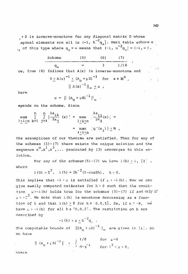
+ D is inverse-monotone for any )
diagonal matrix D whose
.agonal elements are all in (-:\, -2 J h q+ • Next table schov'S a -2 -
t+ of this type where q+ = oo means that (-:\, u q+J = (-:\,"').
Scheme (5) (6) (7)
q+ 00 3 1/18
ow, from (8) follows that A(x) is inverse-monotone and
O<A(x)-1 <(A +lJB)- 1 for - - 0
II A(X) -1
lloo < C1. '
here
a = II (A + lJB) -1 II
0 00
epends on the scheme. Since
n n <laik max /. /, l-ax (x) I = max
1<i<n k=1 j=1 j 1<i<n
<la .. 1-u(x)[
()Xi
e JRn X I
max l<i<n
I q '(x . ) I < M , ~ -
the assumptions of our theorem are satisfied. Then for any of
the schemes (5)-(7) there exists the unique solution and the 0 1 2
sequence x ,x ,x , ... generated by (3) converges to this so-
lution.
For any of the schemes (5)- (7) we have A (h) <A 1 r11 I
where 2
:\ ( 0) = IT , -·2 :\(h) = 2h (1-cosJTh), h > 0.
This implies that -:\ < ll is satisfied if ll > -:\ (h) Now we can
give easily computed estimates for h > 0 such that the condi-
tion jJ>-:\(h) holds true for the sch~es (5)-(7) if and only if
\.1 > -rr 2• We note that :\(h) is monotone decreasing as a func
tion of hand that :\(h)_~8 for heJo,O.Sl. So, if lJ>-8, we
have \.1 > -:\(h) for all he I 0, 0. 51 . The restriction on h are
described by -2
-:\(h) < ll.::. h q+
The computable bounds of li(A + ]JB) -lli are given in Ill. So 0 'I CO
we have
where
II (Ao + \.1 B) -1 II < { 1/8-1
d-jJ
for \.1 =0
. 2 for- n < \.1 < 0,
48
-1 2 d=(lJcos(0.5i3)) , O<i3<II, 11h =2(1-cosi3h)
Now we can easyly see that the condition a 2
MM0
+ aM1 < 1
reduces to the case when a= l/8 for 11 = 0 and a= d- 11-1 for 2
-II <11<0.
REFERENCES
1. BOHLE., LORENZ J.: Inverse monotoniaity and dij'ferenae
sahemes of higher order. A summary for two-point boundary
value problems, Aeg.Math.l9, (1979) ,l-36.
2. HERCEG D.: Iterativno resavanje diskretnog analogona jed
nog nelinearnog konturnog problema. V Znanstveni skup Pro
racunavanje i projektovanje pomocu racunala, Stubicke Top
lice, 1983, 131-135.
3. POPOVIC! P.: An iterative solution of nonlinear finite
differenae equations. An.Univ. Timisoara, seria st.matema
tice, Vol. XX (1982), 49-57.

erical Methods and
Approximation Theory
Nis, September 26-28, 1984
ONE WAY OF DISCRETIZATION OF CHAPLYGIN'S METHOD
Dusan D. Tosic
BSTRACT: ~aplygin's method ( described in [1] and [3] ) is an anartic and iterative method for two-sided approximation to ~e solution of ordinary differential equations. This methi is difficult for practical applications in analytic form. ~ this work one :wa:y of discretization of Chaplygin' s me~od is proposed. Chap11ygin's approximations are calcula-3d by using the interpolation and the numerical integrati-1. Some examples with the cubic spline interpolation and lmpson's rule are presented.
~AN NACIN DISKRETIZACIJE CAPLIGINOVE METODE. Capliginova _3toda ( opisana u [1] i [3] ) je analiticka i iterativna metoda za dvo-stranu aproksimaciju resenja obicnih diferencijalnih jednacina. Ova metoda je teska za prakticne primene u analitickoj formi. U ovom radu pred1ozen 'je jedan nacin diskretizacije Capliginove metodee capliginove aproksimacije se izracunavaju koris6enjem interpolacije i numericke integracije. Navedeni su primeri sa interpolacijom pomo6u kubnih splajnova i integracijom pomo6u Simpsonovog pravila.
1. INTRODUCTTION
Let us consider the initial value problem:
(1) y' = f(x,y), y(a) = y0
e We seek the solution y(x) of (1) on the discrete point set Gh = { xi I xi = a + ih, i=o,. ~. ,n, b-.a = nh } .. Suppose that the sol•ttion of (l) exists and that the conditions for the application of Chaplygin's method are satisfied ( see [1] ). If we denote by uk(x) and vk(x) upper and lower bounding Chaplygin's approximations order k, it holds ( [1] ):
(2) max I uk(x) - vk(x)l < ~ 9 ( C E R+ ) • XE~t~ 2
In [4] and [6] some shortcomings and problems related to Chapligin's method are pointed out. However, if the discretization of Chaplygin's method is made successfully, there
149
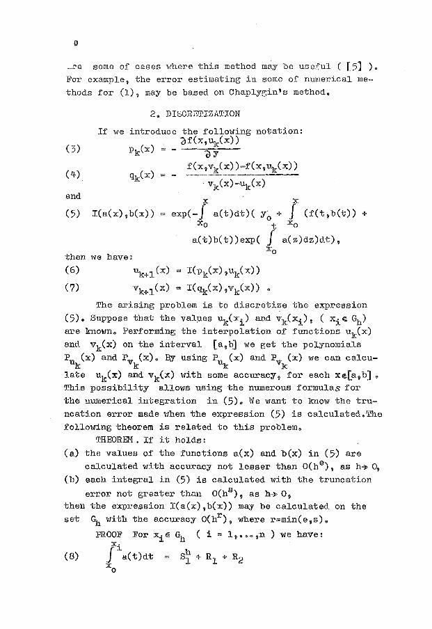
_ . .re some of cases where this method may be useful ( [ 5] ) • For example, the error estimating in some of numerical methods for (1), may be based on Chaplye;in's method.
( 3)
(4)
and
2. DISCRETIZATION
If we introduce the following notation: o f(x, uk(x))
'dY f(x,vk(x))-f(x,uk(x))
= -· vk(x)-uk(x)
(5) I(a(x),b(x)) exp(-f a(t)dt) ( y0
+ f (f(t 9 b(t)) + Xo t Xo
then we have:
a(t)b(t))exp( J a(z)dz)dt), Xo
(6)
(7)
uk+ 1 (x) = I(pk(x), uk( x))
vk+l(x) = I(qk(x),vk(x)) *
The arising problem is to discretize the expression (5). Suppose that the values uk(xi) and vk(xi), ( xi E. Gh) are known. Performing the interpolation of functions uk(x) and vk(x) on the interval [a 9 b] we get the polynomials Pu (x) and Pv (x). By using Pu (x) and Pv (x) we can calcu-
k k k k late uk(x) and vk(x) vtith some accuracy, for each xe.[a, b] .. This possibility allows using the numerous formulas for the numerical integration in (5). We want to know the truncation error made when the expression (5) is calculated.~he following theorem is related to this problem.
THEOREM. If it holds: (a) the values of the functions a(x) and b(x) in (5) are
calculated with accuracy not lesser than O(he), ash~ o, (b) each integral in (5) is calculated with the truncation
error not greater than O(hs), ash~ 0 9
then the expression I(a(x),b(x)) may be calculated on the set Gh with the accuracy O(hr), where r=min(e,s).
PROOF For xi E Gh ( i = 1, ••• ,n ) we have:
(B) ~ia(t)dt = S~ + R1 + R2 xo
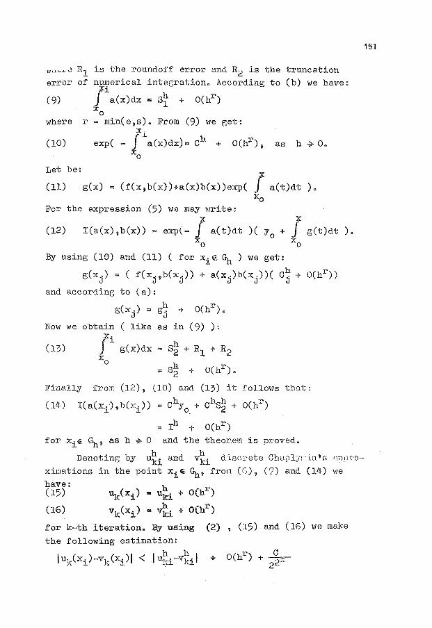
wuvkJ R1 is the roundoff error and R~ is the truncation
error of mu~erical integration. According to (b) we have:
(9) ~1a(x)dx = S~ + O(hr) xo
where r = min(e,s). From (9) we get: x.
(10) exp(- j\~.(x)dx)= ch + O(hr), as h ~o. 0
Let be:
(11) g(x) = (f(x,b(x))+a(x)b(x))exp( ~ a(t)dt ). Xo
For the expression (5) we may 1r1rite: X X
(12) I(a(x),b(x)) = exp(- J a(t)dt )( y0
+ j g(t)dt ). xo xo
By using (10) and (11) (for xie.Gh) we get:
g(xj) = ( f(xj 9b(xj)) + a(xj)b(xj))( C~ + O(hr))
and according to (a):
g(xJ.) = gh + O(hr). j
Now we obtain ( like as in (9) ):
(13) g(x)dx
s~ + O(hr).
Finally from (12), (10) and (l3) it foll0111s that:
(H) I(a(x1.<),b(x;)) = Chy + chsh + O(hr)
.... 0. 2
= Ih ;- O(hr)
for xi e Gh, as h ~ 0 and the theor.em is proved.
DenotinG by u~i and v~i discrete Chu.plyr-:in' s nn-oro
ximations in the point xi~ Gn_, from (6), (7) and (14) we
have: u~i + O(hr) ( 15) uk(xi) =
(16) vk(xi) "' {i + O(hr)
for k-th iteration. By using (2) ' (15) and (16) we make
the following estimation:
h 11 I I uk(xi)-vk(xi)l < I uld -vl~i
151
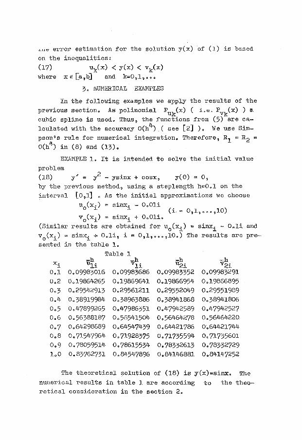
... """' error estimation for the solution y(x) of (1) is based on the inequalities:
(17) uk(x) < y(x) < vk(x) where x E [a,b] and k=O,l,. ••
3. NU!I'JERICAL EXAMPLES
In the following examples we apply the results of the previous section. As polinomial PUk(x) ( i.e. PVk(x) ) a cubic spline is used. Thus, the functions from (5) are calculated with the accuracy O(h4) ( see [2] ). We use Simpson's rule for numerical integration. Therefore, R1 = R2 =
O(h4) in (8) and (13).
EXAMPLE 1. It is intended to solve the initial value problem (18) y' = y2 - ysinx + cosx, y(O) = o, by the previous method, using a steplength h=O.l on the interval [0,1] • As the initial approximations we choose
u (x.) = sinx. - o.Oli 0 ~ ~ (i = 0,1, ••• ,10)
v0(xi) = sinxi + o.Oli.
(Similar results are obtained for u0(xi) = sinxi - O.li and
v0
(xi) = sinxi + O.li, i = 0,1, ••• ,10.) The results are presented in the table 1.
Table 1
v1i -h -h u2i v2i
0.09983686 0.09983352 0.09983291 0.,2 0.19864265 0.19869641 0.19866954 0.19866895 0.3 0.29542913 0.29561211 0.,29552049 0.29551989 0.4 0.38919984 0.38963886 0.38941868 0.38941806 0.5 0.47899265 0.47986)51 o.479Li-2589 0.47942527 0.6 0.56388187 0.56541504 0.56464278 0.56464220 0.7 0,.64298689 0.64547439 0.64421786 o·.644217L~4
0.8 0.71547964 0.71928375 0.71735594 0.71735601 0.9 0.78059514 0.78615534 0.78332613 0.78332729 1.0 0.83762731 0 • 845L~7896 o.8LJ-146881 0.84147252
The theoretical solution of (18) is y(x)=sinx. The numerical results in table 1 are according to the theo-retica1 consideration in the section 2.
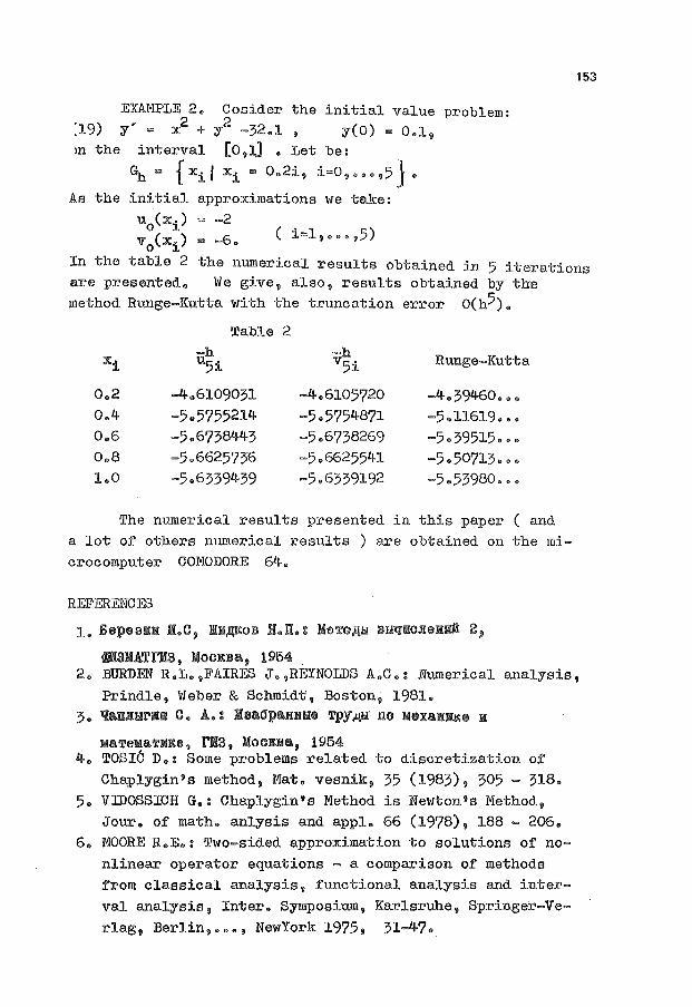
EXA.NPLE 2. Cosider the initial value problem: :19) y' = x2 + y2 -32.1 , y(O) = 0.1, m the interval [0,1] • Let be:
~ = {xi 1 xi= 0.2i, i=0,. •• ,5}.
As the initial approximations we take: u0 (xi) = -2 v0 (xi) = -6. ( i=l,. •• ,5)
153
In the table 2 the numerical results obtained in 5 iterations are presented. We give, also, results obtained by the method Runge-Kutta with the truncation error O(h5).
Table 2
xi -h u5i
-h v5i Runge-Kutta
0.2 -4.,6109031 -4.6105720 -4.39460 ••• 0.4 -5.5755214 -5 .. 5754871 -5.11619 ••• 0.6 -5.6738443 -5.6738269 -5.39515 ••• 0.8 -5.6625736 -5.6625541 -5.50713 ... 1.0 -5.6339439 -5.6339192 -5.53980 •••
The numerical results presented in this paper ( and a lot of others numerical results ) are obtained on the mi-crocomputer COMODORE 64.
REFERENCE3
1. Bepesau I.e, mH~oB H.n.: MeToAH Buqao~e•~ 2, mSIU.TrH3, MooRB& 9 1954
2. BURDEN R.L. 9 FAIRE3 a-. ,REYNOLDS A.C.: Numerical analysis, Prindle, Weber & Schmidt', Boston, 1981.
3 • 'l&Ul:li'BB C • .! • : loa\1paHHii8 Tpy Ali JJO WUUII!te II
W&TeW&TKKe. rls, MoOKDa, 1954 4. TOSIC D.: Some problems related to discretization of
Chaplygin's method, Mat. vesnik, 35 (1983), 305- 318. 5. VIDOSSICH G.: Chaplygin's Method is Newton's Method,
Jour. of math. anlysis and appl. 66 (1978), 188- 206. 6. MOORE R.E.: Two-sided approximation to solutions of no
nlinear operator equations - a comparison of methods from classical analysis, functional analysis and interval analysis, Inter. Symposium, Karlsruhe, Springer-Verlag, Berlin, ••• , NewYork 1975, 31-47.

I
I
,..Jmerical Methods and
Approximation Theory
Nis, September 26-28, 1984
ON A COITVERGE.NCE OF THE DIFFERENCE SCHEMES
FOR THE EQUATION OF VIBRATING STRING
Bosko s. Jovanovic , Lav D. Ivanovic
ABSTRACT:
In this note we inspect the convergence of the difference schemes for the equation of vibrating string, for the case \•Then a generalized solution of the homogeneous boundary value problem belongs to a Sobolev-Slobodetsky space. The results for the elliptic and parabolic case are presented in [2, 3] •
0 KONVERGENCIJI DIFERENCIJSliTH SHENA ZA JEDNACilru ZICE KOJ A TREPERI. U radu se ispituje konvergencija diferencijskih shema za jednacinu zice koja treperi, u slucaju lead e;eneralisano resenje konturnog problema pripada prostoru Soboljeva-Slobodeckog. Analogni rezultati za elipticki i parabolicki slucaj dobijeni su u [2' 3] •
vle wiil consider the first mixed hoElogeneous bounda
ry value problem for the equation of vibrating string:
i'l2
u iu + f(x,t) (x,t) E Q = (O,l) x (O,T) ,
at2 "J} (l) u(O,t) u(l,t) = 0 t E (O,T]
u(x10) = dU(x,O) = 0 X € [0,1] dt
Throught the note we will assume that the generalized solu
tion of (1) belongs to a Sobolev-Slobodetsky space VJ~(Q) ,
1 :$ s ~ 4- , [ 4-]. For such solutions one can construct a li
near extension for t <. 0 remaining in the same class [ 4] . By ll • II s,Q we will denote the norm and by j . 1 s,Q the
senior seminorm in W~(Q) •
define
In the
Pick a nonnegative
a uniform grid wh
same way we define
integer n and let h = 1/n. ':!e
with the step h over (0, 1).
a uniform grid W't" wi-th the step
155

'C" == T/(m+0.5) over (-0.5't',T] Ue vrill assume that c 1 h ~ 't" o::: c2 h , c 1 , c 2 == const > 0
If v is a function defined over Qh'!:' by vj v1e vJill de11ote
restriction for t == (j-0.5)"t'. its 1;Je introduce the difference operators vx, vx' vt
in the standard way [6] • By II · II h and (., • )h we and V:t; will denote the difference analogs of the norm and scalar
product over L2(o,l) . In the space of discrete functions,
which are definecl over Wh and which are equal to zero o
ver the boundary )_mots the operator:
1\v==-vxx
is selfadjoint and positive defin;L te. Therefore the norm
\lvll A-1 == (1\-lv, v)~/2
can be defined. Also the norms over Q \"Till be: h't'
Due to the fact that f(x,t) need not to be continu
ous, it seems natural to approxiE1ate f(x,t) by some mean
values over Qh't". Let T be Steklov' s mollifier defined by:
0.5
T g(x) J g(x + h x') clx'
-0.5
e.nd T 0 g(x) == g(x) Tk g(x) == T(Tk-l g(x)) k==l,2, •••
By Tk,r 'de will clenote the product of Tk over x, llil.cl IJ.'r
over t .
Then v/8 \'Till ap~;roximate ( 1) b;y a weighted cl_ifferG:cl-ce scheEle (a == const > o) :
vt~:-t == a vj+l --'-- (1- 2 a I vj_ - -o vj:l .L rr_2,2 ""j xX I .. XX -.- ~...-~ x:x: r - .L
(2) 0 for X==O and X==l
v 0 v 1 0
'Jhon. u E. 1iJ~(Q) 2 4 6 ' ~ ::: ~ , Ne will clenote z ==
u - v • Function z is v!ell ·defined over Qh't" .s .. tief;;rilJ.t;:

zi-t- = a zj-:J-_1 + (l- 2 a) zj_ + a zxj-x:_l + <fxqx_ + ~~x-:: J v XX · XX -
0 for X=O and X= l '
z 0 u(x,-0.5't"),
z1 u(x, 0.5 "!:),
Hhere
Hhen
T2
' 0 u- v
on u(x,t)
u e W~(Q) , l ~ s ' 3 , we will denote ~ Furthermore, we will assmne that the soluti
can be extended outside Q so that tho ex'censio"1
is odd over x, and remaining in the same class. The functi·-·
on ~ is defined over the grid Qh'l: satisfying:
zj = a ~j!.l + .(l-2 a) zj_ + a zj:l "j tl; XX XX XX + <fxx '
0 for x = 0 and X= l'
T2 ' 0 u(x, -0.5 'C'),
Hhere
q.j = T0 ' 2 uj - T2 ' 0 [a uj+l + (l-2 a) uj +a 11j-l J. Using the method of energy inequalities [6] one cc.~l
prove the follov1ing a priori estimates: m
157
(3) llzll~;~,h ~ C [!iz~llh +II zJ~ + z~ll h + 'C L C ll<f~;:xll h -,-II <Jl.~tll h;J j=l
CL:-) llzii~~.L,h~c (nz~H/\-1 +llzo+z.1
1lh+ 'C'tll<f~llh) J=l
Cehe conver;y:mce rate estimates in this note o.rG ·x>.
o,_:L ·:~;w follor,.rinc generalization of tho Brm.1blo-Hi}_::-, 3rt
LU1l\1A: Let [sr be a nolme::;ative integer, [sr < s :::; + l and let P [sr be t~10 set of pol3rnonio.ls of
c-.1-.::.l over ,:; [sr. If
\1~(0) c.. •
'1 = '1 (u) is a bounded, linear functi-
such that P [sr c: Kernel( ry ) , then fo:;:o
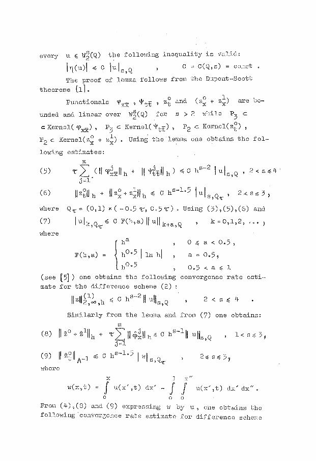
every u. E \v~(Q) the follOi'ling inequalit;y is vulic<.:
l1(u)l ~ C luls,Q C = C(Q,s) = conct •
The proof of lemma follo\·JS from the Dupont-Scott
theoreme [l]. 0
Functionals w .~, - .zt and Txx ' '~'tt '
unded and linear over vl~(Q) for s > 2
(z~ + z~) are bo
while P3
c
cKernel(<pxX), P3
c Kernel('l'tt), P2 c Kernel(z.~),
P2 c Kernel(z~ + z~) • Using the lemma one obtains the fol
lowing estimates:
m
(5) "rL Cll<f~xllh + ll'~'~tllh) ~c hs-2
luls,Q, 2<s~4 j=l
(6) Uz.~llh + llz~+z~llh ~ C hs-l.51uls,Q<t:, 2-<s~3,
where Q'L"= (0,1) x( -0.5 '"C", 0.5"1:'). Using (3),(5),(6) and
(7) I ulk,Q'" ~ C F(h,a) II ull k+a,Q k=O,l,2, ••• ,
where 0 ::; a < 0.5 ,
F(h,a) a = 0.5,
0.5 <. a ~ l
(see [5] ) one obtains the follm'ling convergence rate esti
mate for the difference scheme (2)
llzll~~~,h ~ C hs-2
11 ulls,Q 2 < s ~ 4
Similarly from the lerama and from (7) one obtains:
m
(8) llzo+21
llh + 'LLII<P~cllh::; C hs-lll uiJs,Q j=l
(9)
where
l " -· w(x,t) = J u(x' ,t) dx' - J J u(x' ,t) dx' dx",
0 0 0
From (4-) ,(8) and (9) expressing w by u, one obtains the
following· convergence rate estimate for difference schene
!lzll~~~,h ~ C hs-l Cllulls,Q +llfltp(s),s-1,Q)
1 < s ~ 3, where p ( s) = ma,'C { 0, s - 2 } and II f II P, q, Q
the norm of the anisotropic Sobolev-S1obodetsky space
Vl~'q(Q) = L2
(0,T; W~(O,l)) (\ W~(O,T; L2 (0,l)) (see [4]).
REFERENCES
1. DUPONT T., SC<YrT R.: Polynomial approximation of functi
ons in Sobolev spaces. Math. Comput. 34(1980),4l.J-l-463.
159
2. IVANOVIO L. D., JOVANOVIC B.S., StiLI E. E.: On the convel.'
gence of difference schemes for the Poisson's equation.
IV seminar primijenjene matematike, Split 1984.
3. JOVANOVIC B. S., IVANOVI6 L. ·D., StiLI E. E. : On the rate
of convergence of difference schemes for heat transfer
equation. IV seminar primijenjene matematike, Split 1984,
Ll-o IJIONS J o Lo, MAGENES Eo : Probl8mes aux limites non homo--g~nes et applications I,II. Dunod, Paris 1968.
5. OGANESYAN L. A., RUHOVEC L. A. : Variacionno-raznostnye me
tody reseni:ya ellipticeskih uravnenij. AN ArmSSR, Erevan
1979.
6. SAJV!ARSIITJ A. A. Teori:ya raznostnyh shem. Nauka, Moskva
1983.
Department of Mathematics
Faculty of Sciences
11 000 Belgrade, Student ski trg 16
Yusoslavia

I
I
I
I
I
I
I
I
I
I
I
I

Numerical Methods and
Approximation Theory
Nis, September 26-28, 1984
APPROXIMATION AND m;GULARIZATION OB' CONTROL PROBLE!VI GOVE:CmED BY PARABOJ;IC EQU.'\ TIOJ~r
Lav D. Ivanovi6 , Bosko S. Jovanovic
1\.BSTRACT:
1\. finite dimensional approximation of distributed control Jroblem governed by the heat transfer equation is conside"ed. We prove tha.t a sequence of finite dimensional problem 3olution converge to the original solution. Also, we con -3trv,ct a minimizing sequence which converge to the optimal ~ontrol.
'\.PROKSH'U\.CIJA I REGULARIZACIJ A PROBLEMA OP'l'IMALNOG UPH.,WLJAc!JA ''3IS'l'E!VIIrlfA PAR.il.BOLICKOG TIPA. U ovom radu ::-azmr·1trn se lcona~no dimanziona aproksimacija zadatka outimalnoe urravlja -nja sistemom opisanim jedna~inom provodjenja tonlote. Dokazuje se d2 niz .kona6no dim~nzionih resenja konvcrpira lcr originalnom resenju i vrsl se regulRrizacija tj. konstruise se n:inimiziraju6i niz koji lconvere;ira ka O'JtimalnO!ii upr::•vljanju.
We r:hall consider the follO''Jin,P: nnic'.m~·J. control nro-
blem:
(1) ,T ( V) = ~ f ( U (X , t ) , U (X , t ) ) dxd t _____,... inf "T X U
( 2) ut= 6u + v0
(x,t) E QT=(O,l)2x (O,T]
(3) u(x,t)=O (x,t)E. _s~ X(O,~ -· ') s~ =Co ,1) ~
( 4) u(x,O)= v1
(x)
It is well known[5] that if v0
E. H2r,r(QT)
2r+l(i') . ( ) ( ) (A) v1
E. H .::tc than exlsts a unique solution of 2 , 3 , ....
u E.. E2 (r+l) ,r+l(c;,T) for r ~ 0 and the following estima.te
161

valid:
We shell denote
)<'H2r+l(Q): llv 1\x::::::; R
( ) TJ-[ ex _-r2r,r((', )1'-/ v= v 0
, v 1
and , - v = r- h <; T /
• Throughout the note we sh.c1.ll as-
sume that f is arconvex function and
( 6) lf(a ,a1
,a2)-f(b ~b1 ,-b 2 )\~g(a ,b) ±ja.-b.l
0 0 -..c::: 0 0 1=0 l l
vrhere g:( a , b ) is a T)Osi ti ve bounded function over bounded •' 0 0
sets.
Lemma. The solution of (l)-(4) exists.
Proof. it is easy to show that J(u) is lower weakly
semicontinuous function over U and U is a weaklv compc·ct
set in xr. By [7 Il• 4 7] followG the lemma.
To soJ_ve the problem (l)-(4) we c-.hall construct a
sequence of finite dimensionEJ.l D:roblems of nonlinear l)roo;r2r:1-
ming [ 3 J , [ 7 J Let 2 h be a cmiform grid with the ste!l h=l/n oven·
Q and let Wz be 8 u:ciform grid over ( 0, 'r] vti th the
step rc; =T/m. In this note we shall as~:ume that constent _, 2/ 2
c1
, c2 ~ 0 exists such that c
1 h ~ '?::'::::;;; c
2h •
In the set of discrete functions over 0_ - '2 X') "'117:: - ~~ h u 'L: we sh2.ll introduce the follovvinc; norms:
')tc; II Oo:._,..;
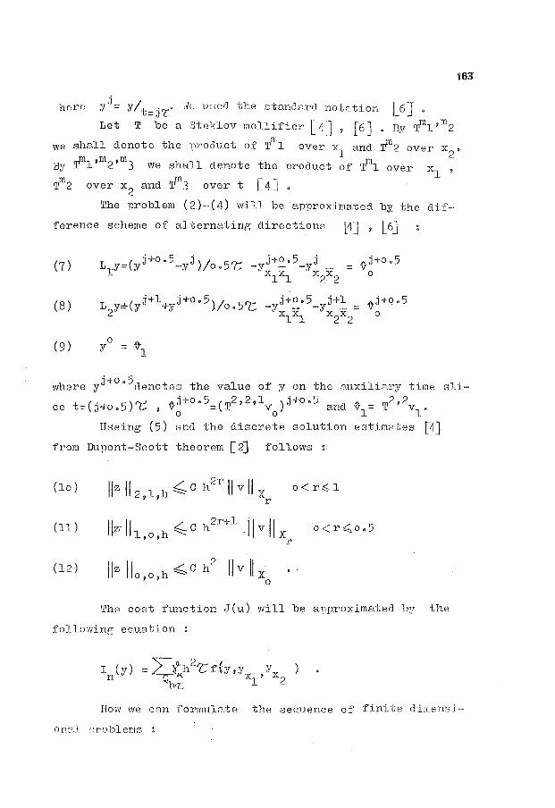
l63
hnrc: y'i= y/t=jrc• }u ur;wJ the stcmc1arr1 not:c.tion [6] •
Let T be a :3teklov mollifi or [ 4 J , [ 6 J • By ~1 'm2
we shall denote the 11rocluct of rrfll1 over x1
and ~2 over x2
•
.JUl,m2,m3 h 11 t .Jil By '1' we s a deno e the product of 'l' 1 over xl ,
?2 over x2
and ?3 over t [4] . The problem (2)-(4) wiD be approximated bY.: the clif-
ference scheme of alternating directions GJ , [6]
(7)
(8)
( 9)
L ...... ( j+l j+o.5)/ 5
rr- j+o.5 j+l 2Y- Y +y o. 0 -y _ -y _ =
xlxl x2x2
0 y = v
1
where yj+o • 5 denot\'lS the value of y on the auxili."'.ry time sli-
t-(. 5 )"t: vj+o.5_(T2,2,1 )j+o.5 1 v _ T2,2 ce - J+o. , 0
- v0
anc. 1
- v1
•
Useing ( 5) and the discrete solution estimEetes [4}
fro1:1 Dupont-Scott theorem [ 2] follows
(lo) liz112,l,h~Ch2rllvllx o<r~l r
(l 2 ) llzllo,o,h~Ch2 lfvllx
0
The cost function J(u) will be a!lproxima.ted b:r the
following equation :
Now we can formulate the sequence of finite dimensi-
on'31 nroblems

(13) I ~ inf n wp,q,s
n
(14) Lly= wo L y= 0 , w y = wl 2 0
where the operators L1
,L2
are defined b~ (7),(8) and the
set wp,q,s= [w=(w w ) r- y =Hp'qx Hs : llw II <:... R} n o' 1 <::::::.. n n n Y ~ n
We denoted by Hp,q Hs the discrete analogues of the Sobolev · n ' n
spaces Hp'q(QT) ,Hs(52.) p,q,s 6 NU{o] . Since (13),(14) is the mathematical programming pro-~
blem one can prove that a solution y * of (13), (14) exists. n
Furthermore we shall construct operators
and P : Y ~X by n n r
Q :X~Y n r n
where w0
E. H2 '1
( QT) and w1 E. n3 (Q)
lants defined in [l] •
are the interpo-
Theorem 1. If the above assumptions are V9lid than
(17)
lim I* = n
n ~oo J* = inf J<u) and for o <r,;; o.5
u
/I~ n
Proof. Useing the technique developed in [ 7] from
(11),(15),(16) one can Prove that the conditions of theorem
3. [7 p.3ll] are satisfied so the theorem 1. follows.
Now, we shall introduce Tichonov functjonnl [7] EJS!
T ( w) = I ( w) + cJ. llvr II Y2~ • n n n n
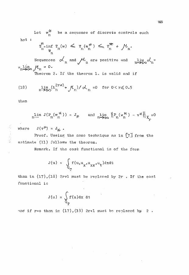
Let w * n hat
*· T =J.nf n w n
Sequences
be a sequence of discrete controls such
T (w) ~ T (w*) ~ T*' + rn· n n n n
ol.n andrn are positive and lim J. = n~OQ n
= lim M. = o. n--"'OC .; -n Theorem 2. If the theorem l. is valid and if
(18) lim (h2r+l+ ){ )/o( =0 for O<r-:::;0.5 n-~oo n .; ·n n
than
lim J ( P ( w ~ )) = J* n- n n
where J(v~) = J* •
Proof. Useing the same technique as in \)] from the
estimate (ll) follows the theorem.
Remark. If the cost functional is of the form
J{u) = J f(u,u ,u ,ut)dxdt Q X XX
T
than in (17),(18) 2r+l must be replaced by 2r. If the cost
functional is
J(u) = S f(u)dx dt QT
ana if r=o than in (17), (18) 2r+l must b8 replaced bd~ 2 •
165

18
REFERENCES
l. CIARLET P,: The finite element method for elliptic prob
lems. North-Holland,Amsterd.am 1978.
2, DUPONT T., SCOTT R.: Pol;,rnomial a-p-proximation of functi
ons in Sobolev spaces. Math. Comput. 34 (l98o),44l-463.
3. EVTUSHENKO Yu.: Metody ·resheniya ekstremaljwrh zadach i ih
primenjenye v sisteme.h optimizi:wii. Nauka ,Moskva 1982.
4. JOVANOVIC B.S. ,IVANOVIC L.D. ,SULI E. E.: On the rate of
convergence of difference schemes for heat transfer equ
ation • IV seminar p:rimijenjene matematike, Split 1984.
5. LIONS J .L. ,MAGENES E.: Non-Homogeneous Boundo.ry Value
Problems and Applications.Springer-Verlag,Berlin 1972.
6, SAMARSKIJ A.A.:Teoriya raznostnyh shem.Nauka , Moskva
1983.
7. VASILJEV F.P.: Metody resheniya ekstremaljnyh zadach,
Nauka,Moskva 1981.
Department of Mathematics
Faculty of Sciences
11 ooo Belgrade, Studentski trg 16
Yugoslavia
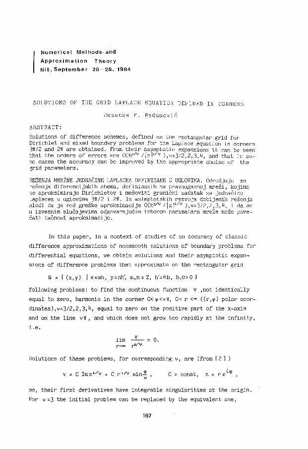
Numerical Methods and
Approximation Theory
Nis, September 26-28, 1984
SOLUTIONS Or THE GRID LAPLACE EQUATION DEfiNED IN CORNERS
Desanka P. Radunovic
ABSTRACT:
Solutions of difference schemes, defined on the rectangular grid for Dirichlet and mixed boundary problems for the Laplace ,equation in corners 3ft/2 and 2ft are obtained. From thejr asymptotic expansions it can be seen that the orders of errors are O(h21" I I z /11 " ) , v=3/2, 2, 3, 4, and that in sone cases the accuracy can be improved by the appropriate choise of the srid parameters.
RESENJA MREZNE JEDNACINE LAPLACEA DEFINISANE U UGLOVIMA. Odredjuju se ~esenja diferencijskih shema, definisanih na pravougaonoj mrezi, kojima se aproksimiraju Dirichletov i mesoviti granicni zadatak za jednacinu japlacea u uglovima 3ft/2 i 2ft. Iz asimptotskih razvoja dobijenih resenja sledi da je red greske aproksimacije O(hVV 1/z/11" ),v=3/2,2,3,4, ida se u izvesnim slucajevirna odgovarajucim izborom parametara rnreze moze pove-6ati tacnost aproksirnacije.
In this paper, in a context of studies of an accuracy of classic
difference approximations of nonsmooth solutions of boundary problems for
differential equations, we obtain solutions and their asymptotic expan
sions of difference problems that approximate on the rectangular grid
n = { (x,y) I x=mh, y=nh', m,n E Z, h'=eh, h,e>O}
following problems: to find the oontinuous function v ,not identically
equal to zero, harmonic in the corner 0< <p<vft, 0< r <"' ((r,<p) polar coor
dinates),v=3/2,2,3,4, equal to zero on the positive part of the x-axis
and on the line vft, and which does not grow too rapidly at the infinity,
i.e.
lim r-.ro
v --= 0 ..
Solutions of these problems, for corresponding v, are (from [2])
v = C Im z 1 /v = C r 1/v sin~ , \)
C - const z -- r e£<p - '
so, their first derivatives have integrable singularities at the origin.
For v =3 the initial problem can be replaced by the equivalent one,
167
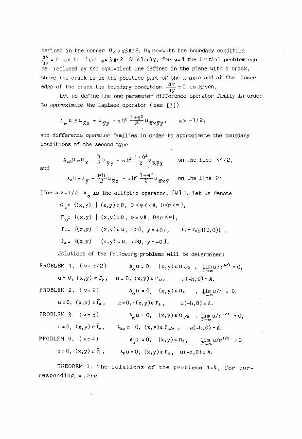
defined in the corner 0 ~ <p d II I 2, o,. r<wvJith the boundary condition
~ = 0 on the line <p = 3 11 I 2. Similarly, for v = 4 the initial problem can ax be replaced by the equivalent one defined in the plane with a crack,
where the crack is on the positive part of the x-axis and at the lower
edge of the crack the boundary condition ~ ~ = 0 is given.
Let us define the one parameter difference operator family in order
to approximate the Laplace operator (see [3])
"l +82
A u = u _ + u _ - CY. h2 - 2- u x-xy-y , CY. - XX yy CY. > -112'
and difference operator families in order to approximate the boundary
conditions of the second type
on the line 3 11 I 2 , and
(for CY. >-1 I 2 ACY. is the elliptic operator, [4] ) . Let us denote
0 = { (x' y) (x,y)e:O, 0 <<p <vii, O<r<"' }, v
r = {(x,y) (x,y)e: n, <p = vll, O<r<oo}, v
fo= {(x,y) (x,y)e:n, x>O, y = +0}' ro = f 0 U{(O,O)} '
r2 = {(x,y) (x,y) e: n, x>O; y = -0 }.
Solutions of the following problems will be determined:
PROBLEM 1. (v=312)
u (-h,O) =A.
PROBLEM 2. (v:2) , limulr = 0, f'-oo
u=O, (x,y)e:r2 , u(-h,O) =A.
PROBLEM3. (v=3)
u=O, (x,y)e:f,, u(-h, 0) =A.
PROBLEM 4. ( v: 4)
>-. u = o, ( x, y) e: r. , u ( -h, o) = A.
THEOREM 1. The solutions of the problems 1-4, for corresponding v ,are
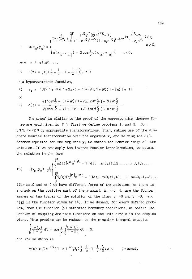
A 211 eLI;[qn(f)e~ml;_1] F( etl;_z
= {""'2~11 F=(,..c.-:_z_1 '") l ( 1 _ e L 1; )' +t/V ( 1 _ z. e t 1; ) t -•/V 1 _ z,. e t I; ) d I;'
n > 0,
u(xm,ylnl) + 2cos~u(x_m,ylnl), n<O,
1ere m = 0, ± 1 , ±2, ... ,
? ) F( z) = 2 F1 ( ~ - ~ , 1 - ~ ; ~ ; z )
3 a hypergeometric function,
1d
4) .J [cos2~ + ( 1 + e•) ( 1 +2a.) sin•~]- e sin~
.J[co&~ + (1+62)( 1+2a.)siri'~ ]+ esin~
The proof is similar to the proof of the corresponding theorem for
square grid given in [1 ]. First we define problems 1. and 3. for
311/2 <<p<211 by appropriate transformations. Then, making use of the dis
crete Fourier transformation over the argument x, and solving the dif
ference equation for the argument y, we obtain the Fourier image of the
solution. If we now apply the inverse Fourier transformation, we obtain
the solution in the form
(5)
211 . I;
lJU.(E;)[qne~m -1Jdf;, m=0,±1,±2, ... , n=0,1,2, ... ,
u(x ,y )=~ 0 m n
211 Jv0 (~;)[qlnlei.ml;_ 1]d!;, m=0,±1,±2, ... , n=-0,-1,-2, ... 0
(for n=+O and n=-0 we have different forms of the solution, as there is
a crack on the positive part of the. x-axis). u0 and v0 are the Fourier
ima5es of the traces of the solution on the lines y = +0 and y = -0, and
q(~;) is the function given by (4). If we demand, for every defined prob
lem, that the function (5) satisfies boundary conditions, we obtain the
problem of coupling analitic functions on the unit circle in the complex
plane. This problem can be reduced to the singular integral equation
1 1 r ...!.i!l dt + cosl!. r~-.!ill.. dt = o, ot-x vo1-xt
and its solution is
- 1 ·• ( ) -11v ( 1 1 1 3 ) 'I' (X ) = C X 1 - X 2 F'1 -2
- - , 1 -- j -2
j X , . v v
C:const.
169
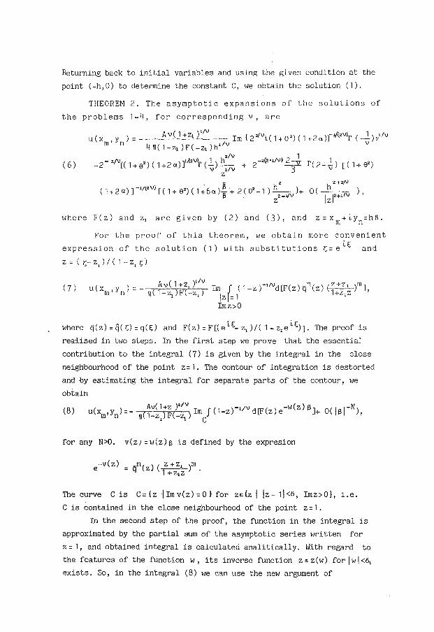
Returning back to initial variables and using the given condition at the
point (-h,O) to determine the constant C, we obtain the solution (1).
THEOREM 2. The asymptotic expansions of the solutions of
the problems 1-4, for corresponding v, are
( 6)
where F(z) and z1 are given by (2) and (3), and z = xm+ tyn=hiL
For the proof of this theorem, we obtain more convenient
expression of the solution (1) with substitutions s=e~C and
z= ( s-z,)/(1-z1 s)
( 7) u(x ,y )=- Av( 1+z,//v Im J (1-z)-1Nd[F(z)qn(z)~)m], m n !1(1-z1 )F(-z1 ) \z\= 1 1+z 1 z
Imz>O
where q(z)=q(s)=q(C) and F(z)=F[(eis_z1 )/( 1-z1 eLs)J. The proof is
realised in tvJO steps. In the first step we prove that the essential
contribution to the integral (7) is given by the integral in the close
neighbourhood of the point z=1. The contour of integration is destorted
and by estimating the integral for separate parts of the contour, we
obtain
( ) Av( 1+z )1fv J ( )-11v ( ) -w(z) ~] (I 1-N)
(8) u xm,yn =-li\i--z )F(-z,.)Im 1-z d[F z e .+ 0 ~ , 1 c
for any N>O. v.(z) = w(z) ~ is defined by the expresion
e-v(z) =
The curve Cis C:{z \Imv{z)=O} for zdz llz-1\<6, Imz>O}, i.e.
Cis contained in the close neighbourhood of the point z=1.
In the second step of the proof, the function in the integral is
approximated by the partial sum of the asymptotic series written for
z= 1, and obtained integral is calculated analitically. With regard to
the features of the function w, its inverse function z=z(w) forlwl<61
exists. So, in the integral (8) we can use the new argument of
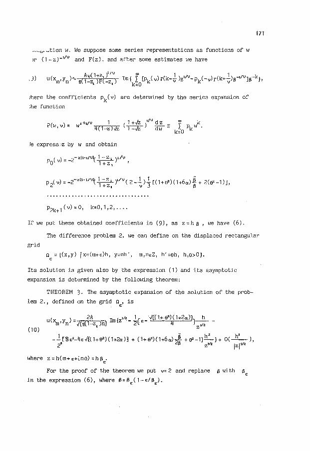
·~~o·~tion w. We suppose some series representaUons as functions of w
>r (1-z)-t/v and F(z). and after some estimates we have
,))
There the coefficients pk ( v) are determined by the series expansion of
;he funcUon
1 +vv 1 1 + ../z 1tv d z "' k P(w,v) = w 4(1-z)Jz (,--:-JZ) CiW = L pkw
k:O
le express ~,z by w and obtain
If we put these obtained coefficients in ( 9), as z = h a , we have ( 6).
171
The difference problem 2. we can define on the displaced rectangular
grid
n ={(x,y) lx=(m+e:)h, y=nh', m,ne:Z, h'=eh, h,e>O}. E
Its solution is given also by the expression (1) and its asymptotic
expansion is determined by the following theorem:
THEOREM 3. The asymptotic expansion of the solution of the prob
lem 2., defined on the grid ne:, is
u( ) _ 2A I { II'> 1{ ../[( l+ e•)(1+2a)]) h xm,yn - ../[ii{1-z
1 )h) m z - 2 _e:-
2v2- -
( 10) 1 . - h 2 h3
-- ['I1Je:2-4e: ../n. 1+82) ( 1+2et)] + ( 1 + 82)\ 1 +6 a) _2_! + e> -1]-} + 0( --),
26 a zY2 jz I s/2
where z=h(m+e:+Lne) =ha. E
For the proof of the theorem we put v= 2 and replace a with ae:
in the expreSSiOn (6), Where a:aE( 1-e:/aE).

From the asymptotic expansion (6) we can conclude that the
accuracy of the approximation is lower when the boundary corner is grea
ter (it depends on v), and that difference schemes of the higher order
accuracy do not provide better approximations. With the choise of <Y., e
and E such as E=../[( 1+ a•)( 1+2<Y.)]/4, the problem 2. can be approximated
in such a way that the order of an error is 0( h2 ) for I zl = 0( 1 ) . For the
scheme with <Y.=-1/6, the choise e::../2 and E::1/(2J2) provides the order
of the accuracy 0( h3 ) •
REFERENCES:
1. AH,L\PEEB B.B.: t'JeTOl!Hhie amrpoKCMM8l.ll1Jil Hei'JIB)lKl1X pemeH!1i1 ,IJ,!1qxpepeHI.1l1a.Jib
Hb~ ypaBHeHl1i1, ~c.~OKT.~l13.-MaT.HayK, MocKBa, 1983.
2. FOX L.,SANKAR R.: Boundary singularities in linear elliptic differen
tial equations, J.Inst.Maths.Applics., 5(1969), 340-350.
3. CAMAPCKl-1 A.A. ,AH,L\PEEB B. B.: PasHOCTHhie MeTO,lU>I ,ll:JJR: GJIJil1ITTl1l!ecKJI!X
ypaBHeHl1i1, HayKa, MocKBa, 1976.
4. THOMEE V.,WESTERGREN B.: Elliptic difference equations and interior
regularity, Numer.Math., 11(1968), 196-210.

Numerical Methods and
Approximation Theory
Nis, September 26-28, 1984
CONNECTION BETWEEN O'm PROBLEM IN ELASTICITY
THEORY AND THE !lfE'l'HOD OF API'ROXDIATE SOLVING
OF CARLEJ-IANN 's BOUNDARY VALUE PROBLEr.f
r.lil os S • Canak
~BSTRACT:
ln this paper we consider one problem in elasticity theory
which appears to be Carlemann 1 s boundary value problem for analitic functions,For approximate solution of Carlemann's
boundary value problem we take the exact solution of corres~ ponding approximate problem and,after that,tve estimate the
error,
VEZA IZHEDJU JEDNOG PIWBLEMA TEORIJE ELM'TICNOSTI I PRIBLIZNOG RESAVANJA GRA1HCNOG PROBLEMA CARLEMANN-A: Razmatra se
jedan problem teorije elasticnosti koji se svodi na granicni problem Carlemann-a za an ali ticke funkcije, Za pribli
zno resenje problema Carlem~n-a uzima se tacno resenje odgovaraju6eg pribliznog probiema,a zatim se daje ocena gre
ske.
In this paper we consider the following problem:
Find such solution of biharmonic equation
(1) y >" 0
which satisfies the following conditions
(2) u(x,O) = 0
0> uytx,o)-O(x)uyy(x,o) ""'h(x) • -oo .(.X<.
173

and which is bounded when y-'?' oa ,if h(x) is a ~iven
continuous function and
-x ff (x) ""ae -x + b
e + c I a, b, c - cons t. I
In this case the function u(x,y) represents the
displacement from the equilibrium position of elastic plate
which covers a halfplro1e and which is fixed along the line
y = 0 by elastic hinge with .a variable stiffness.
If we apply on biharmonic equa.tion
the Fourier transformation
(5)
we get the ordinary differential e~uation
(6)
with general solution
But,if we looking for the particular solution which
satisfies the condition U(x,O)~O and which is bounded
when y ...._,. co , we have that
(8) U(x,y) :=. yC(x)e-1x1y
x>O
x< 0
If we substitute the value of C (x) in the condition
(3) we get that
e-xuy (x, O)+cuy (x, 0} -ae -xuyyLX, o) -buy-}c, o) := e -xh (x)+ch(x)
or,if we introduce the notation

n the condensed form
\17hen '"e apply the Fourier transformation (5) on the
equation (10) it transformes into
(ll) cU lx,O}-bU (x,o)-cH(:x:)=- 4> (:x:+i) y yy
175
Since Uy(x,O):=.C(x) and Uy~x,0)=-21x!C(:x:),substituting
these values into (11) we hawe
(12) C(x}·(c+2blxl) = cH(x)-q, (x+i)
Applicatio~ of Fourier transformation (5) on the re
lation (9) gives
(l)) C (x)·(l + 2a IX I) :::: H (X)+ c:j:» (X)
(14)
Elimination of C(x) from (12) and (13) gives
4> (:x:):- l+ 2a!XI C + 2b lXI
(X+ i)+cH (x)' l + 2a lXI - H(:x:) c+2bl:x:r
Helation (14) represents, so called, Carlemann 1 s boundary
value problem for determining analitic function (z) ,
The most of the theory of Carlemann's boundary value
problem is developed by soviet authors and analitic solving
methods are given in details in [1] •
Nevertheless,in many cases it is more convenient to
apply approximate solving rnethods.In monography [2] pp 156-158, the following theorem, which enab.les approximate solu
tion of problem (l4),is formulated and proved.
'l'l1eorem T: Given the Carlemann' s boundary value prob-
lem
and corresponding approximate problem
(16)
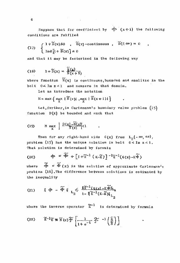
6
Suppose that for coefficient by cp (x+ i) the following
conditions are fulfiled
(17) {
1 + D{x)~O • D(x) -continuous ,
Ind [1+ D(x)] = 0
and that it may be factorized in the following lvay
_. jCx) (18) l+D(x) =(x-1-i)
where function N(z) is continuou~jj,bounded and analit1.c in the
belt 04. Im z <.1 and nonzero in that domain.
Let us introduce the notation
Jl1:::. max{ max I N(x)l ,max I N(x+ 01} X X
Let,further,in Carlemannls boundary value problem (15)
function D(x) be bounded and such that
Then for any right-hand side G(x) from
problem {15) has the unique solution in belt
That solution is determined by fonnula
L2(- «~,eo) I
0 < Im z <. 1.
where ~ "'" ~ (x) is the solution of approximate Carlemann r s
problem (16).The difference between solutions is estimated by
the inequality
(21)
where the inverse operator K-l is determined by formula
(22)

177
~et us now apply the mentioned theorem on the approxi-
tte solving of Carlemann's problem (14) .Instead of the whole
1per halfplane we' 11 obtain only the belt 0-<. Im z-<. 1 and
.• wose,for sake of easier computation, that a r:: 1/2 • b = 1/2
end c -::::: 2. Then Carl emann 1 s boundary value problem (14) appears
·O be
q,(X)+ 1+ lXI cP(X+i) Q 2H(x,.l+\x(_ H(x) 2 + I X/ 2 1- I X I
here function .:P { -:t) has to be anali tic in the belt 0 4 Im z -41
nd for every yE[O,l] satisfies the inequality -24) Js c:P (x+iy)l
2 dx ~ c
The free term G(x) =.2H(x) 2:::tJ!! H(x) 2+Jxl
2 (- oo. oo) .Let us choose in our case that
is given in
""" x2+ 25
1 + D (x) =. x2+ 36, •
/CoP.fficient 1 + D{x) of the approximate problem is choosen
in the form of rational function in order to avoid complicated
computations with Fourier integral.Nore than that,this function
is even,equal to one in infinity and easy to factorize since
it is in form of
For the equation (23) the corresponding approximate e·ua
tion will be
(25)
In order that the equation (25) has the unique solution
it is sufficient /see [2], § 15/ that the following conditions
ore fulfiled
(26) l+D(x)+o
'DC± .oo):::: o Dlx) - continuous
Ind [ 1+ D(x)]::: 0

It is easy to check that all of these conditions hold.
Coefficient by ~ (x+ i) can be factorized in the following
way
(27) 1+ Dtx)
~
where the function N (z) is continuous,bounded and analitic
in the belt 0.(.Im z-<.1 and nonzero iE that domain.ThPn +he
boundary condition (25) by·the substitution
(28) ~ (x) = N(x)· "o/ { x)
where 'f' (x) is new continuous function 9 is transformed into
(29) 'V{x)+'t'(x+i)=2 H(x} N(x+ i)
'"h"'" we apply the inverse Fourier transformation the
equation (29) transformes into 'K
(30) 'i' {x)+e -x. '¥ ( x)"" h (x) -ll 5 [ 2e-6 (x-s~e -5 (x-s) h(s) ds ~GO
Equation (30) gives us the function li' (x) .For determi
ning of function ~ {x) we use relation
01)
WlH"n we apply the inverse Fourier transformation on (31) we
get ~
(32) ~ (x) = 't' (x) -ll S e 6 (x-s) 'f (s)ds
.)(
From formulae (30) and (32) function te (x) may l1e deter
mined by h(x).Now the approximate solution ~(x,y) of problen
(1)-(2)-(3) reduces to the following simplier problem
(33)
(34)
2-Au:::.O
u(x,O): 0
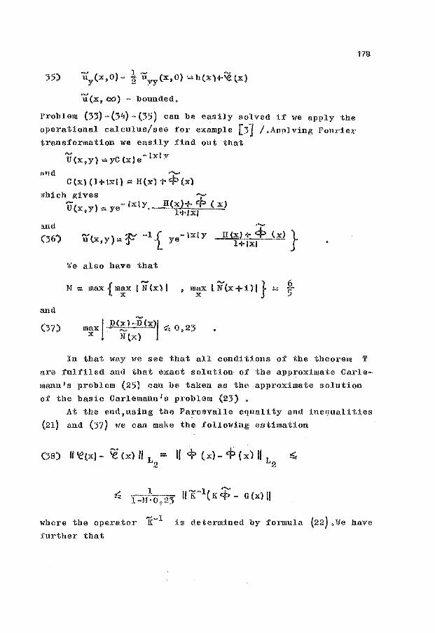
35) - ) 1.... -u (x,o - 2 u (x,o) = h(x)+-'e {x) y yY
u(x, oo) - bounded.
Problem (33)-(34)-(35) can be easily solved if we apply the operational calculus/see for example [3] /.Aonlving Fourier transformation we easily find out that
U(x,y)=yC(x) lxlv
--c {x) (1 +-lxl} = H (x) T c:? (x) ....... i'Thich p;ives
U(x,y} ""ye-IXIY, H(x)+ cp ( x} l<t-lxl
:1nd (36-')
We also have that
and
(37) mp:l D(~)-D(x)I ~ 0,23 N (x)
H (x) +- ~ ( x) } l+lxl
6 = 5
t19
In that way we see that all conditions of the theorem T are fulfiled and that exact solution of the approximate Carlemann's problem (25) can be taken as the approximate solution
of the basic Carlemann 1 s problem (23) • At the end,using the Parcevalle equality and ine~ualities
(21) and (37) we can make the following estimation
(38) II 'e(x) - ~ (x) II L = II ~ ( x)- <fl ( x) II L ~ 2 2
where the operator K:-l is determined by formula (22} .ll'e have
further that

Let us estimate the last integral.
-- 2 ~::~~ H(x)+H(x)] }
2dx = Jnr-1
(x) a~~~~: -2
t- 2 ( X + 25
--x 2+ 36
=(0,23) 2[1 e-t :e (t)+ 2h(t}l 2dt ~g)!)
Using (38), (39) and (4o) we get inequality
(41) \1 'e (x)- ~ {x) II L ~ 0 9 38 II e-x 'e (x) + 2h(x) II 2 L2
..... In order to make functions ~ and ~ even closer to
each other,instead of approximate problem (25) we can take tt
approximate problem in the following form
(42) K'~ :=
'VI
= 2H(x) n 11<."1
2 2 X 4-- Eht - H(x)
with conveniently choosen values for n and ak •
REFERENCES
1. GAHOV F.D.: 11 Kraevie zadaci 11 ,"Nauka 11 ,JI1oslrva,l977. 2. GAHOV F,D,.CERSKII J.I.: 11 Uravnenija tipa svertki",Moskva, 11Nauka 11 ,1978,156-l58. 3. SNEDDON I.: "Preobrazovanija Furje 11 ,Noskva, IL,l955.

rmrnerical Methods and
Approximation Theory
Nis, September 26- 28, 1984
BSTRACT
SOLUTION OF POTENTIAL PROBLEMS WITH INTERNAL SOURCES BY BOUNDARY ELEMENT METHOD
Josip, E. Pecaric, Miodrag M. Radojkovic
he paper presents an alternative proof of the boundary integral formulaion for two-dimensional potential problem with internal sources. This roof appeared to be much simpler than one derived by same authors in [4] nd thus is easier to extend to more complex cases (i.e. three-dimensio-
.. al problems). Accuracy of the method is illustrated by an example.
RESENJE POTENCIJALNOG PROBLEMA SA UNUTRASNJIM IZVORIMA PRIMENOM METODE GRANICNIH ELEMENATA· U radu je prikazan alternativni dokaz integralne granicne formulacije za ravanski potencijalni problem sa unutrasnjim izvorima. Ovaj dokaz je jednostavniji od dokaza koji su isti autori izveli u [4J i stoga ga je lakse prosiriti na slozenije slucajeve (na primer, prostorni problem). Tacnost metode je ilustrovana jednim primerom.
1. INTRODUCTION
Finite difference and finite element techniques were almost exclusively used to solve numericaly the.equations governing the potential problems. Recently it was shown that boundary element method (BEM) can be also applied successfully [1J.
In order to satisfy requirements that usualy arise in practice of solving potential problems, BEM solution procedure must incorporate the solutions of the following problems:
-modelling of sources with finite radii [~ - modelling of coupled subregions with constant material properti-
es [3] . In this paper given is a new simpler proof for the result from [~
concerning modelling of internal sources.
181
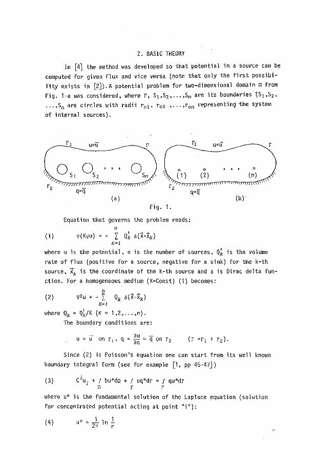
2. BASIC THEORY
In [4] the method was developed so that potential in a source can be computed for given flux and vice versa {note that only the first possibil-ity exists in [2]). A potential problem for two-dimensional domain Q from Fig. 1-a was considered, where r, S1 ,S2, ... ,Sn are its boundaries 1Sl,S2, ... ,Sn are circles with radii r01 , r02 , ... ,r0n repre5enting -the system
of interna~ sources).
{a)
Fig. 1.
Equation that governs the problem reads: n \' , +-+
( 1) 17(K17U) = - t, Qk o(X-Xk) K=1
{b)
where u is the potential, n is the number of sources, Q~ is the volume rate of flux (positive for a source, negative for a sink) for the k-th source, xk is the coordinate of the k-th source and o is Dirac delta function. For a homogeneous medium {K=Const) (1) becomes:
n {2) 112u = - I Qk .s(x-xk)
K=1
where Qk = Q~/K {K = 1,2, ... ,n). The boundary conditions are:
u = u au -on rl' q =an= q on r2
Since {2) is Poisson's equation one can start from its well known boundary integral form (see for example [1, pp 45-47])
(3) ciui + f bu*d~t + f uq*dr = f qu*dr r~ r r
where u* is the fundamental solution of the Laplace equation (solution for concentrated potential acting at point "i"):
(4) u* = _lln l 211 r

183
where r is the distance from the point "i" to any point, ci is a constant from [0,1] (C
1 = 1 for an internal point, ci= 0 for an external point and C
1 = 0,5 for a point on the smooth boundary) and b is known function from Poisson equation. In the case considered:
{5)
Than (3) becomes: n i
(6) c u1 - 1 u~* Q. + ruq*dr = Jqu*dr J J j=1 r r
i.e. n N N
(7) c1u. - I U·~*Qj + I r uq*dr = L f qu*dr ~
j=l J K=l f]c K=l rk
where N is the number of segments used to devide the boundary (boundary elements).
In the case when a 11 Q_js are known one has the case from · [2 ,p. 49]
where the method of superposition was used to solve the problem. But the case from [4] where all Qj are not known can be also obta
ined using (7). If the potential uN+i on s1 is known (see Fig.1-a) one can assume its value on the distance r01 from source and put point "i" on this distance from the source (see Fig.1-b). Now, this is a point inside the domain and c1 = 1 so that (7) becomes:
(8)
{9)
n i* u -"' u.Q. N+i ,L, J J ]=1
For j=i one has: i* 1 1 u. == -ln-~ 211 r 01
N
+ ~ r uq*d K=l rk
N
= 2: rqu*d K=l rk
For j 'f i one can suppose rji » r01 + r0j(rij is the distance between sources i and j) and put:
i* 1 1 u.:::::;- ln-1 211 r .. ( 1 0)
~]
Equations (7) and (8), after selection of the boundary element type .(constant. linear, quadratic, etc. or mixed) [3] can be solved for all unknowns u•s and q's on the boundary rand all unknown u's and Q's for sources (sinks) by solving corresponding system of linear algebraic equa-tions.
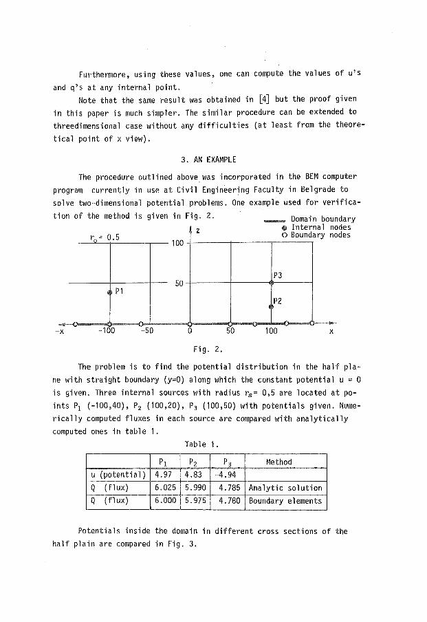
Furthermore, using these values, one can compute the values of u's
and q's at any internal point. Note that the same result was obtained in [4] but the proof given
in this paper is much simpler. The similar procedure can be extended to threedimensional case without any difficulties (at least from the theoretical point of x view).
3. AN EXAMPLE
The procedure outlined above was incorporated in the BEM computer program currently in use at Civil Engineering Faculty in Belgrade to solve two-dimensional potential problems. One example used for verifica-tion of the method is given in Fig. 2.
z r0 "' 0.5
100
50 ~ P1
-x -100 -50 0
Fig. 2.
50
_ Domain boundary
P3
P2
100
• Interna no o Boundary no
l des des
X
The problem is to find the potential distribution in the half plane with straight boundary (y=O) along which the constant potential u = 0 is given. Three internal sources with radius r5 = 0,5 are located at points P1 (-100,40), P2 (100,20), P3 (100,50) with potentials given. Numerically computed fluxes in each source are compared with analytically computed ones in table 1.
Table 1.
pl Pz Pg Method u (potential) 4.97 4.83 -4.94 Q (flux) 6.025 5.990 4.785 Analytic solution
1-::--:---·-· Q (flux)
~----
6.000 5.975 4.780 Boundary elements
Potentials inside the domain in different cross sections of the half plain are compared in Fig. 3.
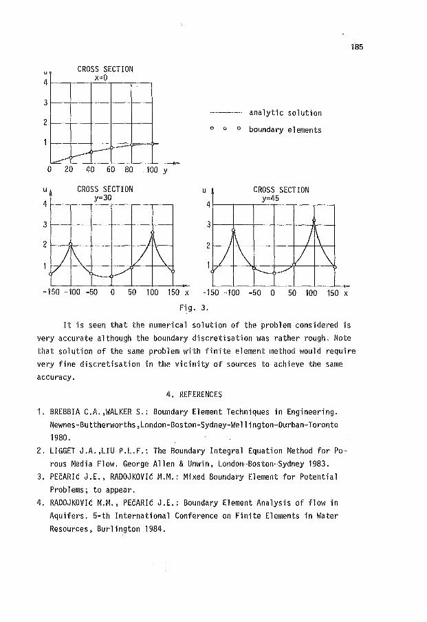
u CROSS SECTION x=O
4
3 analytic solution
2 o o o boundary elements
~ >-_.. v-" 0 20 40 60 80 100 y
u CROSS SECTION u CROSS SECTION
4 y=30
4 y=45
3 3
\ j 1\ J \ I \
I
/ 1\ / \ 2 2
v i'---< )_......... / "" r--..-. / """
-150 -100 -50 0 50 100 150 X -150 -100 -50 0 50 100 150 X
Fig. 3.
185
It is seen that the numerical solution of the problem considered is very accurate although the boundary discretisation was rather rough. Note that solution of the same problem with finite element method would require very fine discretisation in the vicinity of sources to achieve the same accuracy.
4. REFERENCES
1. BREBBIA C.A.,WALKER S.: Boundary· Element Techniques in Engineering. Newnes-Buttherworths,London-Boston-Sydney-Wellington-Durban-Toronto 1980.
2. LIGGET J.A.,LIU· P.L.F.: The Boundary Integral Equation Method for Porous Media Flow. George Allen & Unwin, London-Boston-Sydney 1983.
3. PEcARIC J.E., RADOJKOVIC M.M.: Mixed Boundary Element for Potential Problems; to appear.
4. RADOJKOVIC M.M., PEcARIC J.E.: Boundary Element Analysis of flow in Aquifers. 5-th International Conference on Finite Elements in Water Resources, Burlington 1984.

I
I
I
I
I
I
I
I
I
I
Numerical Me1hcds and
Approximation Theory
Nis, September 26-28, 1984
A POSSIBILITY FOR CALCULATING PRESSURE GRADIENT FORCE
IN SIGMA COORDINATE SYSTEM
Dragutin T. Mihailovic
BSTRACT:
new saheme for the aalaulation of pressure gradient forae n the sigma aoordinate system is proposed. An approximation or the wa term in the thermodynamias equation is aonsidered oo. The proposed method and an earlier approaah {2} is aomared by time-integrations of the atmosphere at rest,
EDNA MOGUCNOST ZA IZRACUNAVANJE SILE GRADIJENTA PRITISKA U IGMA KOORDINATNOM SISTEMU. Predlozena je nova 8ema za izra
uunavanje siZe gradijenta pritiska u sigma koordinatnom sistemu. Razmatrena je jedna aproksimaaija za wa clan u jednaaini termodinamike. Predlozeni metod i jedna ranije predlozena aproksimaaija {2} pgrdjene su pomoau vremenskih integraaija za sZuaaj mirne atmosfere.
1. INTRODUCTION
The problem of calculating pressure gradient force in
the sigma coordinate system is well known. It is related to
the appearance of two terms in the expressions for the pres
sure gradient force. For example, with the original sigma coo
rdinate {8} over a sloping terrain the two terms in the exp
ressions of the pressure gradient for9e tend to be large in
absolute value and have opposite signs. If, say, they are in
dividually ten times greater then their sum, a 1% error in
temperature (2-3°C) will result in a 10% error in the pressu
re gradient force {9}. To overcome this problem, a number of
difference analogues of the pressure gradient force in the
sigma coordinate system have been developed {2},{1},{3}. A
problem encountred by some of these analogues when geopoten
tial is initially specified rather than temperature has rece
ntly been discussed by Mesinger { 5} 'and compared by a numeri-
187
cal example of the atmosphere at rest {6},
In this paper we shall concentrate our attention to the
possibility of calculating the pressure gradient force in the
sigma coordinate system by means of an interpolation proce
dure. In addition, we shall try to approximate in finite-dif
ference form, the wa term that provides consistent transfor
mation from potential to kinetic energy. Finally, the propo
sed schemes was compared with an earlier one {2}.
2. METHOD OF CONSTRUCTION
Notation
ap specific heat at constant pressure
k suffix indicating level of the model
p pressure
R gas constant
a suffix indicating surface value
t suffix indicating atmosphere top value
T temperature
V lateral vector wind
u,v components of V
a specific volume
cr (p-pt)/(p8-pt) the vertical coordinate
a dcr/dt
11
w Pa-Pt dp/dt
~ geopotential
V f:f lateral del operator in "sigma" surfaces
Vp lateral del operator in "pressure" surface
In the sigma coordinate system, the differential form
of the pressure gradient force has the form
( 1) - V ~ = - V ~ - RTV11 p CJ
Starting from this expression, Kurihara {4} proposed a
technique for calculating the pressure gradient force in the
sigma coordinate system. Namely, it is possible to minimize
the error in the calculation of pressure gradient force by
interpolating geopotential from the nearest sigma surfaces to
constant pressure surface. This idea was applied to vertical~
ly non-staggered grid with velocity components, temperature
and geopotential defined in the middle of the layers.
Kurihara's idea can also be applied in the case of the
staggered grid in the vertical, with geopotential located at
the interfaces of the layers. This decision seems more reaso
nable since the latter grid is a better choice then the for
mer one {10}. In our case we used quadratic interpolation in
accordance with the hydrostatic equation in the form
(2) RT p
Let us add that in the case of a more realistic atmo
sphere anversion) we can apply the spline method of interpo
lation using all levels of the atmosphere model.
For a number of pressure gradient force schemes an as
sociated procedure for calculation the wa term of the thermo
dynamic equation,
(3) ~at (11a T) + 'i/ (11Va T) + ~(11c'w T) o p rJ p orJ p
11wa
ensuring consistency of the transformation between kinetic
and potential energy, has been developed. Experiance has
shown that it is desirable to preserve the consistency even
in numerical models designed for short-range simulations.
Otherwise, numerical instability may be encountred in less
than a day of simulation time, in the presence of steep topo
graphy especially.
The contribution to the generation of kinetic energy
by the pressure gradient force can be written in the form
(4) 11wa
It was stated already ·that the exact cancelation, in the fi
nite-difference form should be provided between the wa terms
in (3) and (4).
189

Taking into account the continuity equation, hydrosta
tic equation, and w, we arrive at
(5) 11Wct - ~(11~0) - ~(~cr)~ - ~v •11V + RTp~V•V 11 a cr 'f a a 'f at 'f cr ap cr
Comparing the right sides of the expressions (4) and
(5), that must be equal and in the finite-difference form, we
find that the divergence of the surface pressure should be
calculated via the expression
(6)
In this way we cancel the wa terms in (3) and (4) in the ex
pression for total energy.
Using the thermodynamics equation (3), hydrostatic eq
uation (2) and definitio of w, we can write
(7) wa
In the finite-difference form, the last expression,
for the case of horizontally staggered variables, in the x
direction, has the form
(8}
where
(9)
and o and o are operators of divergence in the finite-x,p x,cr difference form in x direction for p=const. and cr=const. The
subscript 0 denotes the point where the contribution of the
wa term is calculated; 11* denotes the value of 11 in the point
in which velocity components are not defined.

3. A NUMERICAL EXAMPLE
We copmared the proposed scheme with an earlier appro
tch {2} which includes a non-staggered distribution of vari
ables in the vertical.
The experiment consisted of time-integrations with an
atmosphere in a hydrostatic equilibrium; motions generated
are thus a consequence of the pressure gradient force error
(Blumber, personal comunication). The integrations were per
formed in a two dimensional domain (x,a) with constant boun
dary conditions specified at the western boundary (x=O). At
the eastern boundary (x=l2000 km) the radiation boundary con
dition was used {7}. Atriangular mountain with 500 km width
and the maximum height of 2 km was defined in the midlle of
the domain. The atmosphere was devided into nine layers in
the vertical. The initial surface pressure was 1000 mb away
from the mountain. The top of the model atmosphere was at
200 mb. A strong inversion up to 900 mb was located on the
left of the mountain; the temperature was 0°C at 900 mb and
-10°C at 1000 mb. Otherwise a temperature profile linear in
Znp was assumed, the temperature taking on the value 3.5°C
at 1000 mb and o0 c at 900 mb. The exact initial geopotential
was calculated integrating the given temperature profiles.
The grid size was 250 km, time step 10 min, and Coriolis par
ameter 0.0001 s-l
days 0 1 2 3 4 5 6 7 8 9 10 11
c 18.49 6.08 5.61 5.49 5.55 5.42 5.42 5.40 5.47 5.48 5.53 5.51
I 0.39 0.39 0.41 0.42 0.43 0.44 0.46 0.47 0.48 0.50 0.51 0.53
daysO 1 2 3 4 5 6 7 8 9 10 ll
c 8.92 5.40 5.12 4.84 4.68 4.60 4.41 4.32 4.20 4.10 3.99 3.93
I 0.32 0.32 0.33 0.34 0.35 0.36 0.38 0.39 0.40 0.42 0.43 0.44
Table 1. RMS pressure gradient force error, in terms of geostrophic wind,
for different schemes, and for the wind point nearest the moun-
tain at its "inversion" side (above) and its "no inversion" si-
de (below).
191

(because of the system symmetry V::::V(r ); V:fcV(z) and ;1V/i'Jz:o0)
and blllll!d~ou>;~r condition V:=O fo:t." :t'""F!, BJ1d may l1e o'btained r)y con~
ventional application of the image theorem" Following this theo
rem the electro
static sys·i;em (the orJ.ginal
q ::cw'J :LtG image
::d; the cUrectio:
J) oa:n l><::l u.seda
So the eleot:r:.ic scalar
(3) G "' ln
is so c~alled Green~ s
tes, E. irJ the electric
dx·ical coo:l;di
3. A NEW INTJ.!aU'HE1'ATIOH 01<1 Tli8
'rhe equation ( 1 ) can be also solved
of integral transform method [2]: .roll
Consider Laplace's equation l 1.'
r ?f:i) + or
Di
var:Lani
0
and assume the potential solut:tun :Lu the
V = R(r) F(~) ~ where
va:ri.able fo1
(4)
and k is the separable consta,nt to be detex:'minedo 'rhe solutions dife:cential equations (4) are ek~ and e~l{€1> and cl(r
and sl(:c):c.:sin(ldn~), rco::!pe(;t Fed;
and dete:cmining k0
so tbe fnnctJona ol ( and
sln(:l•):c:sin(nlc0ln~) satisfJ.ed condHion~ b Jo, for nlm
(5) J cln(r)clm(r)rdr = l and a Tl
~2k ( 1 +d ) ~ for n==m •0
no
b f0 9 for n~m and n=O or m=O
( 6 ) J sl ( r) sl ( r) dr_ "' ~ a n m r 1
1
Ji: for 0 l2~~ 9
where b > a, we have k0

195
~xpending Dirac's {~function f(r-d) in the series
(7) r f ( r-d) "' f 2 sln ( r) sln ( d) n= 1 - ln ( b/ a r , for a ( d < b ,
we have in the case when b-..<'.,
(8) rJ(r-d) = t S sin(pln£)sin(pln~)dp c
0 a a
Because of the obtained Dirac's J -function integral transform~;ttion the solution of Poisson's equation (1) can be written as
, 00 sin(plni)sin(pln~)
(9) V = rr l p sh(pJr) ch[e-,UYL)p]dp
wher 11 + 11 is for O~e~ J.. and "-" is for J...{; e ~ 2J( •
3. APPLICATION OF PRESENT RESULTS, EXEMPLES AND CONCLUSION
The physical solution of the consider problem is independent to the mathematical approach. So the solutions (2) and (9)
are equal and we have the following expression: V(from formula 2), V(from formula 9). Using series
( lO) ch(e-JtJL)p = fl p[e-o{±ll-(2m+1 )1Z] + -p[_e-oL±Ji+(2m+1 )JZ] sh(px) ~ e e
oo m-o 2 2 and integral J 1 -c~spA e-pBdp = ~ln~ , forB> o, we have froJ
o B last. expression
= ln2(L2d)+ [e-Jtit-(2m+1 )il] 2
(11) jl a _ d2
r 2+a4-2a2rd cos(e-d)
m"'-oo ln2 (~) + [e-J.±JI-( 2m+1 )JL] 2 - a 2 [r2+d2-2rd cos( e-~U v·here a~r<=, at;,d and with"+" for O~et;,d.. and 11
-11 for J.~e~2'i[.
Puting in (11) 'r=e-J , R=r/a ~ 1, IJ::::d/a ~ ·1 or RD=eA, A?. O, and
R/D=eB, B is optional, we have:
( 12 ) P= fl ln2
(RD)+(Y-'-2mRi m=-oo ln2(R/D)+('f'-2m.il) 2
( 13)
Separately, we have:
R2D2+1-2RDcos't' "' R2+D2-2RDcos 'f'
Q<l A 2+~m2Jt2 _
B shfA~2~ ( 14) P(= n , for '1'=0, m=l B2+4m2Jl2 - A sh B 2
( 15) P2= n C2tm 2 _ shgW) , for 'f=O, A=2JlC and m=1 ~- Jl
m
""
and
B:;::O and
c2 +(2m-1~ 2 2 (16) P3= n , for 'f='Sl/2, A=JrC/2 and D2+( 2m.,:.1 )2
= B=KD/2 • m=1

The obtained formulas are very useful, because of the sloVlJ convergence of present infinite products. The convergence of products shown folloving numerical results (Approximate values are calculated by multipling 65 membres of infinite products. The exac values are in brackets.): For R=2, Il=2 and If=- 51:' P = 1.55783 (exact P"" 1.5625). For R=2, Il=4 and lf=-.1! P = 2.24039 (exact P = 2.2500). For R=2, D=2 and r=-JV6 P = 9.36901 (exact P = 9.93971143). For R=2, Il=2 and ~=-2JL/3 P ~ 1.74477 (exact P = 1.7500).
In the following table the exact values of P2 for different c are shown.
f
--a ----r----- 1?~------ -------c---1- ----p-2 __ _ ----o~---- ~-1.6oooooo66 - 2;---:- ----,f~2612923:E+OT-
o. 01 II 1. 000164501 5. : 2.112184 71!:+05 0.1 1.016530706 10. 1 7.0078318£+11 0.5 I 1.465052383 I 20. l 1.5428269E+25
L'_·--~-6?~~~791 0 _l_~ ?~·- __ _I __ 5. 2682~?5~~~5 -Combinig the results (16J for 0=1 with known formula
00
P; = n ( 1- ~ ) = ~ , we have m=2 m
noo 1 shR P4 = (1--;r) = :pr- =
m=2 m "' 0.9190194776.
REFERENCES
1. SURUTKA J.V.: Elektromagnetika, Gra~evinska knjiga, Beograd 1965.
2. VELICKOVIC D.lli.: Metodi za proracun elektrostatiiSkih polja, Stil, Podvis, 1982.
3. GRADSTAJN I.s., RIZIK I.I>:.: Tablici integralov, sum, rjadov proizvedenia, Izdatelstvo "Nau:ca 11 , Moskva 1971.

Numerical Methods and
Approximation Theory
Nis, September 26-28, 1984
VALUATION OF SEVERAL SINGULAR INTEGRALS USING ELECTROSTATIC FIELDS LOWS
Dragutin M. Veli~kovi6
BSTRACT:
sing electrostatic fields lows a special approach to the seve~1 singular integrals evaluating is presented. The obtained rellts are useful in numerical solution of electrostatic problems
u3 integral equations technique.
ODREBIVANJE NEKIH SINGULARNIH INTEGRAL! POMOGU ZAKONITOSTI ELEKTROSTATICKIH POLJA: Koriscenjem odredenih elektrostatickih zakona izvraeno je izracunavanje ocredenog broja singularnih integrala. Dobijeni rezultati su od koristi u toku pribli~nog·numeri~kog resavanja integralnih jedna~ina elektrostatike.
1. INTRODUCTION
In the applied electromagnetic field theory we have often necessary to compute several kin~of integrals having singular subintegral functions. Special in the case when field pointb are in the region of electromagnet'ic field sources. Because of the singularity of subintegral functions conventional numerical quadrature formulas are not useful, except after the singularity extraction. The present paper shown an effective method for evaluating several kinds of singular integrals. In the present method sssence is the application of several electrostatic field lows, in the first place conformal maping and logarithmic potential theory. Except general theoretical description, two separate examples are shown. The obtained results are very useful for numerical solution of electrostatic integral equations systems. So we have the excelent numerical results in the theory of stripe lines.

2. EVALUATION OF SINGULAR INTEGRALS
We consider planparallel electrostatic field with knovn1 but arbitrary cross section (Fig.1).
v~ VV=f(Z.)
X u - ... --
z-plane w-plane Fig.l F'ig. 2
For electric scalar potential evaluation two general p! cedure exist:
1? In the case when the surface charges densities on tl:
electrode, ~(r~), are known, the potential, v, is:
{
u, for r E: si' si is conductor interior
(l) V(r) := u- 21c j1<r')d1 9ln(\r-r'l/lro-r'l), for rE se I
88
is conductor exterior, where c is the contour of conductor cross section,£ is electrJ permitivity, U is the conductor potential and q'== ~7(i:')d1' '
c the conductor total charge per unite length.
2? The second way for potential evaluating is based on conformal maping. If we have the complex function w:::Rej't' = u+j, == f ( z=rej 8 =x+j y) , j = v:1 , which map the exterior of conducto: z-plane to the unite circular cylinder exterior in w-plane (Fj the complex potential is
( 2 ) <j) = f U , :f~r R ~ 1
Lu- 2~£ lnw = V+jlf, :for R~1. During conformal maping the electrode potential and total linE charge densities are constant.
The real part of ¢ is potential, ( 3 ) V = Re { ¢>} = U - 2-ii: lnR • The electric field on the conductor surface is E=\d~/dzl = = q' \w~ \I2.JLE , where I w~ I= \dw/ dz I for R=1. U!'Jing boundary cone tion )? =E:E we have (4) 1 := % I Wb I
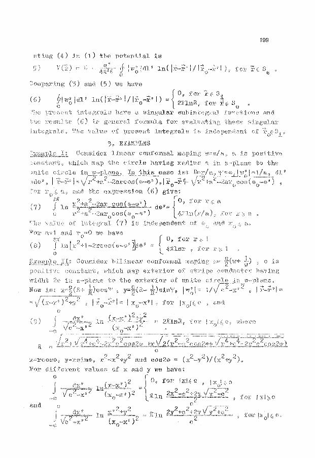
199
uting (4) in (1) the potentlal iB
~ lw' jrn 9 1n( lr-r 1' 1/lr e o < ~"
0) and (5) we have
( 6) I/ { 0 9 for I' E S "l
' I ) "' 2JilnB. 9 :tor ii E- S 0
singular suld"Id;c f'PYJ :l"o:ns R:ncl.
rn'nmla :tor EnraJua"t.:ing
3 EXAMPMS
C'onside~L' Unear conform~l
2ft:
(7) J ln
Ji'o:t' 2!1
(8) J 0
Co:nside:r b:U coni:o:rmal m
mro>.p End;erior
o tho exterior of
:lr'"l'COSE) 9
Fox· d1ffc:cenl; va.lues of
and eos20 = (
x and y we have~
J n o~g""""~"'~~2 ,~ { 0 for I :>:t: 10 e
Jlln
e
and
ln
en 9