Embed Size (px)
Citation preview

Numerisk Analys, MMG410. Lecture 4.
1 / 38

Matrisfaktoriseringar: LU-faktorisering
Ax = b loses i de tre stegen:
1 Berakna L (undertriangular matris) och U (overtriangularmatris) sa att A = LU. For att losa LUx = b infor vibeteckningen z = Ux och far da problemet Lz = b.
2 Los Lz = b (framatsubstitution).
3 Los Ux = z (bakatsubstitution). Framatsubstitution gar tillpa samma vis som bakatsubstitutionen fast man tar raderna iomvand ordning.
Kostnad?
A = LU tar ungefar n3/3 vardera av + och ·.Lz = b kostar n2/2 vardera av + och ·.Ux = z kostar lika mycket (n2/2).
2 / 38

LU-faktorisering for linjara ekvationssystem
Vad ar det for fordel med detta jamfort med vanligGausselimination ?Svar: enklare att hantera vid teoretiskt arbete.Det gor det ocksa mojligt att effektivt losa problem av typenAxk = bk dar bk+1 beror av xk .Om alla hogerleden ar kanda pa en gang kan givetvis vanligGausseliminationutnyttjas.Man loser ett sadant problem sa har:
Berakna L och U sa att A = LU.
Los LUxk = bk , k = 1, 2, ....
3 / 38

Gaussian EliminationThe Algorithm — uniqueness of factorization
Definition
The leading j-by-j principal submatrix of A is A(1 : j , 1 : j).
Theorem 2.4.
The following two statements are equivalent:1. There exists a unique unit lower triangular L and non-singularupper triangular U such that A = LU.2. All leading principal submatrices of A are non-singular.
4 / 38

Gaussian EliminationThe Algorithm — uniqueness of factorization
Proof.
We first show that (1) implies (2). A = LU may also be written
[A11 A12
A21 A22
]
=
[L11 0L21 L22
]
×[U11 U12
0 U22
]
=
[L11U11 L11U12
L21U11 L21U12 + L22U22
]
where A11 is a j-by-j leading principal submatrix, as well as L11 andU11. ThereforedetA11 = det(L11U11) = detL11detU11 = 1 ·∏j
k=1(U11)kk 6= 0,since L is unit triangular and U is triangular.
5 / 38

Gaussian EliminationThe Algorithm — uniqueness of factorization
Proof.
(2) implies (1) is proved by induction on n. It is easy for 1-by-1matrices: a = 1 · a. To prove it for n-by-n matrices A, we need tofind unique (n-1)-by-(n-1) triangular matrices L and U, unique(n-1)-by-1 vectors l and u, and unique nonzero scalar η such that
A =
[A bcT δ
]
=
[L 0lT 1
]
×[U u0 η
]
=
[LU LulTU lTu + η
]
By induction unique L and U exist such that A = LU. Now letu = L−1b, lT = cTU−1, and η = δ − lTu, all of which are unique.The diagonal entries of U are nonzero by induction, and η 6= 0since 0 6= detA = det(U) · η.
6 / 38

Matrisfaktoriseringar: LU-faktorisering
Example
A =
[2 64 15
]
; L−? U−? A = LU
A =
[a11 a12a21 a22
]
=
[ℓ11 0ℓ21 ℓ22
]
·[
u11 u120 u22
]
=
[u11ℓ11 ℓ11u12ℓ21u11 ℓ21 · u12 + ℓ22 · u22
]
ℓ11 · u11 = a11 ⇒ L =
[1 0
ℓ21 1
]
7 / 38

Rakna LU-faktorisering.
8 / 38

Example
⇒ u11 =a11ℓ11
= a11
ℓ11 · u12 = a12 ⇒ u12 = a12
ℓ21 · u11 = a21 ⇒ ℓ21 =a21u11
=a21a11
=4
2= 2
ℓ21 · u12 + ℓ22 · u22 = a22 ⇒ 2 · a12 + 1 · u22 = a22 ⇒
u22 = a22 − 2 · a12 = 15− 2 · 6 = 3[2 64 15
]
︸ ︷︷ ︸
A
=
[1 02 1
]
︸ ︷︷ ︸
L
·[2 60 3
]
︸ ︷︷ ︸
U
9 / 38

Ar LU-faktorisering en stabil algoritm?
Har foljer en grov skiss som visar vad som kan ga fel. Lat ε sta forett litet tal, a1, a2 och a3 markerar “medelstora” tal.LU-faktorisering blir da:
[ε a2
a1 a3
]
︸ ︷︷ ︸
A
=
[1 0
a1/ε 1
]
︸ ︷︷ ︸
L
[ε a2
0 a3 − a2(a1/ε)
]
︸ ︷︷ ︸
U
a1/ε blir ett stort tal, vilket ger utskiftning i berakningen avu22 = a3 − a2(a1/ε). Lat oss anta att hela a3 skiftas ut och att alltannat raknas ut exakt. Hur stort blir bakatfelet?
[1 0
a1/ε 1
]
︸ ︷︷ ︸
L
[ε a2
0 −a2(a1/ε)
]
︸ ︷︷ ︸
skifted U
=
[ε a2
a1 0
]
︸ ︷︷ ︸
faktoriserad matris
Vi har alltsa faktoriserat en matris som avviker mycket fran A i(2, 2)-elementet. Algoritmen behover inte vara stabil.
10 / 38

Ar LU-faktorisering en stabil algoritm?
Det kan vi dock latt fixa. Kasta om raderna i systemet (byt ordning paekvationerna), dvs. studera matrisen B = PA:
B =
[0 1
1 0
]
︸ ︷︷ ︸
P
[ε a2
a1 a3
]
︸ ︷︷ ︸
A
=
[a1 a3
ε a2
]
LU-faktorisering blir nu:[
a1 a3
ε a2
]
=
[1 0
ε/a1 1
]
︸ ︷︷ ︸
L
[a1 a3
0 a2 − a3(ε/a1)
]
︸ ︷︷ ︸
U
Notera att ε/a1 ar ett litet tal. Vi far alltsa inte farlig utskiftning i u2,2.Lat oss anta att a3(ε/a1) skiftas ut:
[1 0
ε/a1 1
]
︸ ︷︷ ︸
L
[a1 a3
0 a2
]
︸ ︷︷ ︸
skifted U
=
[a1 a3
ε a2 + a3ε/a1
]
︸ ︷︷ ︸
fakt. matris
= B +
[0 0
0 a3ε/a1
]
11 / 38

Row echelon form
In the case of Gaussian elimination the pivot eliments should not be zero.Interchanging rows or columns in the case of a zero pivot element isnecessary.In linear algebra a matrix is in row echelon form if
All nonzero rows (rows with at least one nonzero element) areabove any rows of all zeroes [All zero rows, if any, belong at thebottom of the matrix]
The leading coefficient (the first nonzero number from the left, alsocalled the pivot) of a nonzero row is always strictly to the right ofthe leading coefficient of the row above it.
All entries in a column below a leading entry are zeroes (implied bythe first two criteria).
This is an example of 3× 4 matrix in row echelon form:
1 a1 a2 a30 2 a4 a50 0 −1 a6
12 / 38
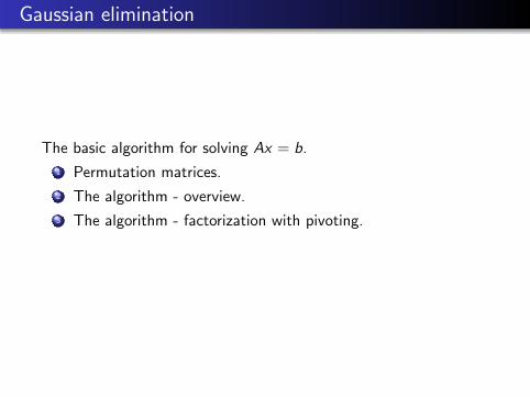
Gaussian elimination
The basic algorithm for solving Ax = b.
1 Permutation matrices.
2 The algorithm - overview.
3 The algorithm - factorization with pivoting.
13 / 38

Permutation matrices
Definition
Permutation matrix := identity matrix with permuted rows.
Example
1 0 0 00 1 0 00 0 1 00 0 0 1
14 / 38

Permutation matrices
Definition
Permutation matrix := identity matrix with permuted rows.
Example
1 0 0 00 1 0 00 0 1 00 0 0 1
→0 0 1 01 0 0 00 0 0 10 1 0 0
→
15 / 38

Permutation matrices
Definition
Permutation matrix := identity matrix with permuted rows.
Example
1 0 0 00 1 0 00 0 1 00 0 0 1
→0 0 1 01 0 0 00 0 0 10 1 0 0
→0 0 1 00 0 0 10 1 0 01 0 0 0
16 / 38

Permutation matricesProperties
Properties of permutation matrices (P , P1, P2):
P · X = same matrix X with rows permuted
P1 · P2 is also a permutation
P−1 = PT (reverse permutation)
det(P) = ±1 (+1 for even permutations, -1 for odd)
17 / 38

Gaussian EliminationThe Algorithm — Overview
Solving Ax = b using Gaussian elimination.
1 Factorize A into A = PLUPermutation Unit lower triangular Non-singular upper triangular
18 / 38

Gaussian EliminationThe Algorithm — Overview
Solving Ax = b using Gaussian elimination.
1 Factorize A into A = PLUPermutation Unit lower triangular Non-singular upper triangular
2 Solve PLUx = b (for LUx) :
LUx = P−1b
19 / 38

Gaussian EliminationThe Algorithm — Overview
Solving Ax = b using Gaussian elimination.
1 Factorize A into A = PLUPermutation Unit lower triangular Non-singular upper triangular
2 Solve PLUx = b (for LUx) :
LUx = P−1b
3 Solve LUx = P−1b (for Ux) by forward substitution:
Ux = L−1(P−1b).
20 / 38

Gaussian EliminationThe Algorithm — Overview
Solving Ax = b using Gaussian elimination.
1 Factorize A into A = PLUPermutation Unit lower triangular Non-singular upper triangular
2 Solve PLUx = b (for LUx) :
LUx = P−1b
3 Solve LUx = P−1b (for Ux) by forward substitution:
Ux = L−1(P−1b).
4 Solve Ux = L−1(P−1b) by backward substitution:
x = U−1(L−1P−1b).
21 / 38
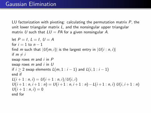
Gaussian Elimination
LU factorization with pivoting: calculating the permutation matrix P , theunit lower triangular matrix L, and the nonsingular upper triangularmatrix U such that LU = PA for a given nonsingular A.
let P = I , L = I , U = Afor i = 1 to n − 1find m such that |U(m, i)| is the largest entry in |U(i : n, i)|if m 6= iswap rows m and i in Pswap rows m and i in Uif i ≥ 2 swap elements L(m, 1 : i − 1) and L(i , 1 : i − 1)end ifL(i + 1 : n, i) = U(i + 1 : n, i)/U(i , i)U(i +1 : n, i +1 : n) = U(i +1 : n, i +1 : n)−L(i +1 : n, i) U(i , i +1 : n)U(i + 1 : n, i) = 0end for
22 / 38

Forward substitution
The next algorithm is forward substitution. We use it to easily solve agiven system Lx = b with a unit lower triangular matrix L.
Forward substitution: solving Lx = b with a unit lower triangular matrixL.
x(1) = b(1)for i = 2 to n
x(i) = b(i)− L(i , 1 : (i − 1)) x(1 : (i − 1))end for
23 / 38
Backward substitution
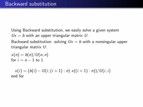
Using Backward substitution, we easily solve a given systemUx = b with an upper triangular matrix U.
Backward substitution: solving Ux = b with a nonsingular uppertriangular matrix U.
x(n) = b(n)/U(n, n)for i = n − 1 to 1
x(i) = (b(i)− U(i , (i + 1) : n) x((i + 1) : n))/U(i , i)end for
24 / 38

LDU-faktorisering
Vi bildar givetvis aldrig permutationsmatriserna utan rader flyttasvia tilldelning eller pekare.
Definition
LDU-faktoriseringenL har ettor pa diagonalen. Kan fa ettor pa U:s diagonal genom att“bryta ut” U:s diagonal (antar A ickesingular).
Example
Har ett exempel dar vi struntar i pivotering for att slippa brak.
[2 6
4 15
]
︸ ︷︷ ︸
A
=
[1 0
2 1
]
︸ ︷︷ ︸
L
[2 6
0 3
]
︸ ︷︷ ︸
U0
=
[1 0
2 1
]
︸ ︷︷ ︸
L
[2 0
0 3
]
︸ ︷︷ ︸
D
[1 3
0 1
]
︸ ︷︷ ︸
U
Sa allmant A = LDU. Vi kan utnyttja detta for att titta pa tvaviktiga fall:
25 / 38
LDU-faktorisering
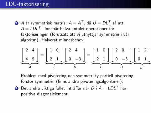
1 A ar symmetrisk matris: A = AT , da U = DLT sa attA = LDLT . Innebar halva antalet operationer forfaktoriseringen (forutsatt att vi utnyttjar symmetrin i varalgoritm). Halverat minnesbehov.
[2 4
4 5
]
︸ ︷︷ ︸
A
=
[1 0
2 1
]
︸ ︷︷ ︸
L
[2 4
0 −3
]
︸ ︷︷ ︸
U
=
[1 0
2 1
]
︸ ︷︷ ︸
L
[2 0
0 −3
]
︸ ︷︷ ︸
D
[1 2
0 1
]
︸ ︷︷ ︸
LT
Problem med pivotering och symmetri ty partiell pivoteringforstor symmetrin (finns andra pivoteringsalgoritmer).
2 Det andra viktiga fallet intraffar nar D i A = LDLT harpositiva diagonalelement.
26 / 38

Matrisfaktoriseringar: DU-faktorisering
A =
[a11 a120 a22
]
⇒ A = DU, D − diagonalmatrix
[a11 a120 a22
]
=
[d11 00 d22
]
·[
1 u120 1
]
d11 · 1 = a11 ⇒ d11 = a11
d11 · u12 = a12 ⇒ a11 · u12 = a12 ⇒ u12 =a12a11
d22 · 1 = a22
Rakna DU-faktorisering for
A =
[2 60 3
]
27 / 38

Rakna DU-faktorisering for
A =
[2 60 3
]
28 / 38

Example
A =
[2 60 3
]
=
[d11 00 d22
]
·[1 u120 1
]
d11 = 2; d22 = a22 = 3; u12 =a12
a11=
6
2= 3
A =
[2 60 3
]
=
[2 00 3
]
︸ ︷︷ ︸
D
·[1 30 1
]
︸ ︷︷ ︸
U
29 / 38

Example: Choleskyfaktorisering
[4 8
8 25
]
︸ ︷︷ ︸
A
=
[1 0
2 1
]
︸ ︷︷ ︸
L
[4 8
0 9
]
︸ ︷︷ ︸
U
=
[1 0
2 1
]
︸ ︷︷ ︸
L
[4 0
0 9
]
︸ ︷︷ ︸
D
[1 2
0 1
]
︸ ︷︷ ︸
LT
=
[1 0
2 1
]
︸ ︷︷ ︸
L
[2 0
0 3
]
︸ ︷︷ ︸
D1/2
[2 0
0 3
]
︸ ︷︷ ︸
D1/2
[1 2
0 1
]
︸ ︷︷ ︸
LT
=
[1 0
2 1
]
︸ ︷︷ ︸
L
[2 0
0 3
]
︸ ︷︷ ︸
D1/2
︸ ︷︷ ︸
C
[2 0
0 3
]
︸ ︷︷ ︸
D1/2
[1 2
0 1
]
︸ ︷︷ ︸
LT
︸ ︷︷ ︸
CT
= CCT .
30 / 38

Choleskyfaktorisering
A = CCT kallas Choleskyfaktorisering och den existerar nar A arsymmetrisk A = AT och positivt definit:
x 6= 0, xTAx > 0.
Man kan visa att LU-faktorisering for en positivt definit matris arstabil aven om vi inte pivoterar.Positivt definita matriser ar vanliga i tillampningar.
31 / 38

Example
Vi har partiklar med massorna m1,m2,m3 och farterna v1, v2, v3. Dentotala kinetiska energin, Ekin ar
m1v21 +m2v
22 +m3v
23
2=
1
2
[v1 v2 v3
]
︸ ︷︷ ︸
V T
m1 0 0
0 m2 0
0 0 m3
︸ ︷︷ ︸
M
v1
v2
v3
︸ ︷︷ ︸
V
=VTMV /2.Ekin > 0 om nagon massa ror sig, dvs. om V 6= 0 och V TMV > 0 sa attM ar positivt definit.
32 / 38

Theorem
En symmetrisk, positivt definit (s.p.d) matris har positivaegenvarden. Omvandningen galler ocksa: en reell, symmetriskmatris A ar positivt definit om den har positiva egenvarden.
Proof.
En reell och symmetrisk matris A har reella egenvarden ochegenvektorer.
Ax = λx
daxTAx = λxT x
och
λ =xTAx
xT x> 0
ty xT x =∑n
k=1 x2k > 0 k > 0 eftersom x inte ar nollvektorn.
33 / 38

Matrisfaktoriseringar: Choleskyfaktorisering
Choleskyfaktorisering for s.p.d. A ar A = L · LT , var L arundertriangular matris.
[a11 a12a21 a22
]
=
[ℓ11 0ℓ21 ℓ22
]
·[ℓ11 ℓ210 ℓ22
]
=
[ℓ211; ℓ11 · ℓ21ℓ21 · ℓ11; ℓ221 + ℓ222
]
.
ℓ11 = 1, ℓ21 = a21;
ℓ221 + ℓ222 = a22
a221 + ℓ222 = a22
ℓ22 =√
a22 − a221 > 0
[a11 a12a21 a22
]
︸ ︷︷ ︸
A
=
[1 0a21 ℓ22
]
︸ ︷︷ ︸
L
·[1 a210 ℓ22
]
︸ ︷︷ ︸
LT
34 / 38

Matrisfaktoriseringar: Choleskyfaktorisering A = L · LT
A =
[a11 a12a21 a22
]
︸ ︷︷ ︸
A
=
[ℓ11 0ℓ21 ℓ22
]
︸ ︷︷ ︸
L
·[
ℓ11 ℓ210 ℓ22
]
︸ ︷︷ ︸
LT
=
[ℓ211; ℓ11 · ℓ21ℓ21 · ℓ11; ℓ221 + ℓ222
]
.
ℓ211 = a11 ⇒ ℓ11 =√a11
ℓ11 · ℓ21 = a12 ⇒ ℓ21 =a12ℓ11
=a12√a11
ℓ21 · ℓ21 + ℓ22 · ℓ22 = a22
ℓ221 + ℓ222 = a22 ⇒ ℓ22 =√
a22 − ℓ221 =
√
a22 −a212a11
;
Rakna Choleskyfaktorisering A = L · LT for
A =
[4 88 25
]
;
35 / 38

Rakna Choleskyfaktorisering A = L · LT for
A =
[4 88 25
]
;
36 / 38

Example
A =
[4 88 25
]
;
Ar A s.p.d. ? Raknar egenvarden:
λ1 ≈ 1.3 > 0λ2 ≈ 27.7 > 0
⇒
ℓ11 =√a11 =
√4 = 2; ℓ21 =
a12√a11
= 82 = 4; ℓ22 =
√
25− 82
4 = 3.
A = L · LT =
[2 04 3
]
·[2 40 3
]
37 / 38

Cholesky algorithm:
for j = 1 to nljj = (ajj −
∑j−1k=1 l
2jk)
1/2
for i = j + 1 to nlij = (aij −
∑j−1k=1 lik ljk)/ljj
end forend for
Here, dimA = n. If A is not positive definite, then (in exactarithmetic) this algorithm will fail by attempting to compute thesquare root of a negative number or by dividing by zero; this is thecheapest way to test if a symmetric matrix is positive definite.
38 / 38