Embed Size (px)
Citation preview

國立交通大學
資訊科學與工程研究所
碩士論文
適應性的自動回歸模型的增加畫面更新率轉換方法
An Adaptive Auto-Regressive Model for Frame Rate
Up-Conversion
研究生:王世明
指導教授:蔡文錦 博士
中華民國 99 年 11 月

適應性的自動回歸模型的增加畫面更新率轉換方法
An Adaptive Auto-Regressive Model for Frame Rate Up-Conversion
研 究 生:王世明 Student:Shih-Ming Wang
指導教授:蔡文錦 Advisor:Wen-Jiin Tsai
國 立 交 通 大 學
資 訊 科 學 與 工 程 研 究 所
碩 士 論 文
A Thesis
Submitted to Institute of Computer Science and Engineering
College of Computer Science
National Chiao Tung University
in partial Fulfillment of the Requirements
for the Degree of
Master
in
Computer Science
Nov 2010
Hsinchu, Taiwan, Republic of China
中華民國九十九年十一月

i
誌謝
在這兩年多的研究所生涯中,能完成我的碩士論文,首先最要感謝的就是我
的指導教授蔡文錦博士。在學業研究上,孜孜不倦地與我討論各種相關的議題,
點出我研究上的盲點,引導我前往正確的方向;在日常生活中,不時的關心我給
予我前進的力量。在此向我最敬愛的指導教授蔡文錦博士,致上最高的敬意。
我要感謝實驗室的學長姐,周鼎力、陳建裕、林宜政、吳漢倫、林詩凱、黃
子娟,謝謝你們指導我各種研究上的相關知識。另外要感謝我的同學們,潘益群、
許智為、游顥榆、溫善淳,謝謝你們陪伴我度過這段追求知識的過程,課業上的
互相砥礪,生活中的互相打氣,讓我從你們身上獲益良多。還有謝謝學弟妹們,
張育誠、吳佳穎、呂威漢、謝寧靜,謝謝你們讓我在研究所生涯中過得更加精采,
祝福你們順利畢業。
最重要的,感謝我的家人們,尤其是我的母親,在背後默默支持我,讓我在
疲累的時候有一個溫暖的避風港,謝謝你們對我有所期待及付出。最後謝謝我的
女朋友呂蕙茹,謝謝有你一路上的陪伴以及信任。
接下來要告別學生生涯,進入職場了,大家珍重。
謹以此論文獻給我的師長、家人及所有關心我的朋友們

ii
中文摘要
增加畫面更新率是視訊處理中眾多議題的其中之一。本篇論文提出
了一種適應性的自動回歸模型,使其產生的畫面有更好的視覺品質及
更少的計算負擔。在傳統的自動回歸模型中,每個像素被建模為時間
上像素點或空間上像素點的線性組合。而在本論文中,我們提出了一
個利用視訊資料的特性來選擇回歸模型的機制。選擇適當的回歸模型,
可以在回歸運算當中減少不必要的變數,在計算複雜度上得到了相當
程度的改善。實驗結果顯示出在運算時間上得到了顯著的進步,並且
在內插出的畫面中,視覺效果也得到了改善。
關鍵字: 適應性的自動回歸模型、增加畫面更新率

iii
ABSTRACT
An adaptive auto-regressive model is proposed in this thesis for frame rate
up-conversion. In conventional AR model, each pixel in the to-be-interpolated frame is
modeled as a linear combination of temporal neighborhood, spatial neighborhood, or
joint temporal-spatial neighborhood pixels. This thesis proposed a temporal AR model
(called TAR) utilizing temporal neighborhood; and a spatial AR model (called SAR)
utilizing spatial neighborhood. Besides that this thesis also proposed a scheme which
selects TAR or SAR adaptively according to motion information in the video sequence.
By selecting appropriate AR model, unnecessary variables can be eliminated from
regression process. Compared to STAR model [2] which utilizes joint temporal-spatial
neighborhood for each pixel, computational cost can be greatly reduced with the
proposed method. In addition, the experiment results show that visual quality can also
be improved by adaptively adopting appropriate AR models for frame interpolation. The
results demonstrate the superiority of the proposed method in regarding to improved
visual quality and reduced computational cost.
Index Terms----Frame rate up-conversion, adaptive auto-regressive model

iv
CONTENTS
口試委員會審定書 ........................................................................................................... #
誌謝 .................................................................................................................................... i
中文摘要 ........................................................................................................................... ii
ABSTRACT .................................................................................................................... iii
CONTENTS .................................................................................................................... iv
LIST OF FIGURES ....................................................................................................... vi
LIST OF TABLES ......................................................................................................... vii
Chapter 1 Introduction ............................................................................................. 1
Chapter 2 Related Works .......................................................................................... 5
2.1 MC-FRUC ...................................................................................................... 5
2.2 STAR model ................................................................................................... 6
2.3 Flow chart of STAR model .......................................................................... 11
Chapter 3 Proposed Method ................................................................................... 13
3.1 Motivation .................................................................................................... 13
3.2 TAR Model ................................................................................................... 15
3.3 SAR Model ................................................................................................... 17
3.4 Model Selection Criterion ............................................................................ 18
3.5 Flow chart of proposed method .................................................................... 21
Chapter 4 Experimental Results ............................................................................ 22
4.1 Environment ................................................................................................. 22
4.2 Model Parameters ......................................................................................... 22
4.3 Objective Quality ......................................................................................... 23
4.4 Subjective Quality ........................................................................................ 28

v
4.5 Time complexity ........................................................................................... 30
Chapter 5 Conclusion .............................................................................................. 34
REFERENCE ................................................................................................................ 35

vi
LIST OF FIGURES
Figure 2-1 : Bi-directional motion estimation diagram. Each block is assumed to be
experienced a translational motion. ................................................................ 5
Figure 2-2 : STAR model diagram. Each pixel is modeled as a linear combination of its
temporal and spatial neighborhood (As called support region). .................... 7
Figure 2-3 : Self-feedback algorithm diagram .................................................................. 9
Figure 2-4 : The flow chart of STAR model with self-feedback weight training. .......... 11
Figure 3-1 : The 2nd
to-be-interpolated frame of the test sequence Mobile_CIF. Left-top
corner marked window A with color blue, and middle-down marked window
B with color red. ........................................................................................... 14
Figure 3-2 : Weight distribution in window A and B of 2nd
to-be-interpolated frame of
the test sequence Mobile_CIF. ..................................................................... 14
Figure 3-3 : ATAR diagram. ............................................................................................ 15
Figure 3-4 : ASAR diagram. ........................................................................................... 17
Figure 3-5 : The validity of selection criterion of the test sequence Foreman_QCIF. ... 19
Figure 3-6 : The validity of selection criterion of the test sequence Mobile_CIF .......... 20
Figure 3-7 : Flow chart of proposed method Proposed_AST. ........................................ 21
Figure 4-1 : Frame by frame PSNR of Foreman_QCIF ................................................. 24
Figure 4-2 : Frame by frame PSNR of Mobile_CIF ....................................................... 26
Figure 4-3 : Frame by frame PSNR of Football_CIF ..................................................... 27
Figure 4-4 : Foreman_CIF 4th
interpolated frame. (a) FA (b) MCI8x8 (c) STAR (d)
Proposed_AST ............................................................................................. 29

vii
LIST OF TABLES
Table 4-1 : PSNR table of FRUC algorithms. ................................................................. 27
Table 4-2 : PSNR table of regression-based FRUC algorithms ...................................... 28
Table 4-3 : Model selection ratio .................................................................................... 31
Table 4-4 : Execution time comparison between STAR and Proposed_AST (support
order = 1) ...................................................................................................... 32

1
Chapter 1 Introduction
Frame rate up-conversion (FRUC) one of the main issues in video data
transmission. To transmit huge amount of video data, the spatiotemporal resolution of
video signals is often reduced to achieve the limited bitrate. In temporal domain, video
frames may be skipped for lower bitrate, which also degrades the visual quality at the
decoder side. To restore the skipped frames, FRUC algorithm must be performed at the
decoder side as a post-processing stage.
The FRUC can be used in low bitrate video coding by transmitting the half amount
of original video frames, and performing FRUC algorithm at the decoder side. FRUC
can also be applied in other applications. The most practical one is format conversion
(For example, from PAL of format 25 frames/s to NTSC format of 30 frames/s). FRUC
also provides a great help in slow-motion playback with higher visual quality.
Meanwhile, many FRUC algorithms have been developed. The common solutions
without extra efforts is to produce the frame by using co-located pixel value in previous
temporal neighborhood (frame repetition, FR), or by combining two temporal
neighborhood co-located pixels value (frame average, FA). Though these algorithms
provide an efficiency performance, they ignore the motion information in video data,
and therefore, results in the visual quality degraded (for example, blurring) in motion

2
part of video. Another kind of FRUC algorithms is developed to overcome such effects.
These algorithms are referred as motion compensated FRUC (MC-FRUC). The frame
interpolation in MC-FRUC is along with the motion trajectory to achieve better visual
quality. Given the correct motion vectors, MC-FRUC outperforms the FR/FA algorithms.
Many motion estimation (ME) algorithms have been developed to increase the accuracy
of motion vectors. Conventional methods such as block matching algorithm (BMA)
have been broadly applied in FRUC. Choi et al. [1] proposed bi-directional motion
estimation, which produces more faithful motion vectors for FRUC.
Different from ME process in video coding, the ME in FRUC is performed without
available pixels of target frame. Hence, the derived motion vectors may not be
consistent sometimes, resulting in the block artifacts or the jerky motion. Although
block artifacts can be reduced by performing overlapped block motion compensation
(OBMC)[1] after motion compensated interpolation(MCI), the interpolated frame may
still look unpleasant sometimes.
Auto regressive (AR) model has been applied in many image processing
applications, such as detecting and interpolating “dirt” areas in image sequences [3],
ME [4], super-resolution [5], forecasting video data [6], may give us inspiration using
AR model in FRUC issue. Yongbing Zhang et al. [2] proposed a spatial-temporal auto
regressive model (STAR) for FRUC. Each pixel in STAR is modeled as spatial

3
neighborhood and temporal neighborhood’s linear combination. Using an iterative
self-feedback weight training algorithm can derive accurate weighting coefficients for
STAR model. The STAR model is able to consider the non-stationary statistics of video
signal, and thus can resolve the challenging issue such as zooming, panning, and
non-rigid objects.
Although the STAR model can achieve quite well visual quality, the computation
complexity is inevitably high. The STAR model with self-feedback weight training’s
computation complexity is proportional to four to the power of its regression model’s
variable number. The model assumes that every pixel is related to temporal and spatial
neighborhood, and the weighting coefficients analysis in [2] states that the pixel with
high motion may have more connection with spatial neighborhood. We proposed a new
regression-based schema for FRUC with two different AR models and a model selection
criterion. Using adaptive temporal auto-regressive model and adaptive spatial
auto-regressive model with adaptive selection can reach better performance both in
computation efficiency and visual quality.
The following of this thesis is organized as follows. First, a brief introduction of
the related works, including the traditional MCI with bi-directional motion estimation
and STAR model with self-feedback weight training is given. Then, proposed method is
presented, which describes the proposed spatial AR model, temporal AR model, and

4
how to adaptively select AR models properly. Experimental results are provided in
section 4, and last, the conclusion is summarized at final section.

5
Chapter 2 Related Works
2.1 MC-FRUC
MC-FRUC can achieve better visual quality than frame average by exploiting the
motion redundancy between frames. The figure 2-1 shows the overall architecture of
bi-direction motion compensated interpolation.
Figure 2-1 : Bi-directional motion estimation diagram. Each block is assumed to be
experienced a translational motion.
First the to-be-interpolated frame is divided into non-overlapping blocks. For each
block, the bi-direction motion search is performed. The bi-direction motion search will
find a motion vector v for block B(i, j) by minimizing the bi-directional sum of square
error (SBSE) in the search window.
The bi-directional motion search can be interpreted by
SBSE,B(i, j), 𝑣- = ∑ (𝐹𝑡−1,𝑠 − 𝑣- − 𝐹𝑡+1,𝑠 + 𝑣-)2
𝑠∈𝐵(𝑖,𝑗)
( 1 )

6
𝑣𝑖,𝑗 = 𝑎𝑟𝑔𝑚𝑖𝑛𝑣
*SBSE,B(i, j), 𝑣-+
( 2 )
, where S is a 2-D vector representing a pixel location, the 𝐹𝑡−1, 𝐹𝑡, and 𝐹𝑡+1denote the
previous, to-be-interpolated, the following frames, respectively. The 𝑣𝑖,𝑗 represents the
bi-direction motion search’s result for block B(i,j) in to-be-interpolated frame 𝐹𝑡. After
the motion search, we then use the motion information to interpolate the block. Also,
to-be-interpolated block B̂(i, j) in 𝐹𝑡 is given by (3).
B̂(i, j) =1
2{𝐹𝑡−1[𝑆 − 𝑣𝑖,𝑗] + 𝐹𝑡+1,𝑆 + 𝑣𝑖,𝑗-}
( 3 )
S represents the pixels’ locations of B̂(i, j). Each pixel in B̂(i, j) is an average of
pixels at motion compensated location in previous frame and following frame. The (3)
shows the main assumption of MCI with bi-directional motion estimation (Bi-MCI).
Each block is assumed to experience a translational motion. The blocking artifacts will
arise if the adjacent blocks experience significantly different motion vectors, or the
object is non-rigid aligned the block.
2.2 STAR model
Spatial-Temporal auto-regressive model (STAR) is proposed in [2] to enhance the
visual quality of the interpolated frames. It models each pixel as a linear combination of
its temporal and spatial neighborhood. First, frames are divided into non-overlapping

7
area with size WxxWy, said training window R. Assuming each pixel in a training
window is interpolated by corresponding spatial-temporal neighborhoods using the
same weighting vector �⃗⃗� . Using least square method, the best fitting weighting vector
can be solved. The STAR model is illustrated in figure 2-2.
Figure 2-2 : STAR model diagram. Each pixel is modeled as a linear combination of its
temporal and spatial neighborhood (As called support region).
Each pixel in to-be-interpolated training window can be formulated as ( 4 )
R̂t−1( k, l ) = ∑ ∑ Rt−2(k + u, l + v)
v) ≤L
× Wp(u, v)
−L≤(u,
+ ∑ ∑ Rt(k + u, l + v)
v) ≤L
× Wf(u, v)
−L≤(u,
+ ∑ ∑ R̂t−1(k + u, l + v)
*v=0,−L≤u<0+
× Ws(u, v)
*v<0,−𝐿≤𝑢≤𝐿+∪
( 4 )
where R̂t−1 is the to-be-interpolated training window; and Wp , Wf, Ws represent the
weights of temporal neighborhood in the previous frame, the weights of temporal
neighborhood in the following frame, and the weights of spatial neighborhood,
respectively. The L is defined as spatial-temporal support order (support order, for short).
When L is set to 1, the pixel is modeled as the weighted sum of 9 pixels in previous

8
frame, 9 pixels in following frame, and 4 pixels in current frame. The (k, l) represents
the pixel location within the training window. The (u, v) represents looping index for
each element in spatial-temporal neighborhood, called support region. The optimal
solution for weighting vector is, the one that minimizes the distortion ε between training
windows R̂t−1 and Rt−1 to have best fitting weighting vector.
ε = 𝐸( Rt−1 − R̂t−1) = ∑ ∑ 𝐸 [.Rt−1(𝑘, 𝑙) − R̂t−1(𝑘, 𝑙)/2
]𝑊𝑦
𝑙=0
𝑊𝑥
𝑘=0
( 5 )

9
Since the actual pixel values in the to-be-interpolated frame are not available in
FRUC (In (5), for example, Rt−1), equation (5) can’t be used for deriving correct
weighting coefficients. An iterative method, called self-feedback weight training loop
algorithm was proposed with STAR model to deal with such issue. The self-feedback
weight training loop consists of two parts. The pixels in training windows R̂t−1 and
R̂t+1 are first interpolated by using their spatial-temporal neighborhood with the
weighting vector �⃗⃗� , which consists of each element of Wp, Wf, and Ws, rewritten in 1-D
manner. Then, the pixels in R̂t−1 and R̂t+1 are used to approximate the training
window R̂t using the same weighting vector �⃗⃗� , as illustrated in figure 2 – 3 and the
equation (6) below.
Figure 2-3 : Self-feedback algorithm diagram
R̂t( k, l ) = ∑ ∑ R̂t−1(k + u, l + v)
v) ≤L
× Wp(u, v)
−L≤(u,
+ ∑ ∑ R̂t+1(k + u, l + v)
v) ≤L
× Wf(u, v)
−L≤(u,
+ ∑ ∑ R̂t(k + u, l + v)
*v=0,−L≤u<0+
× Ws(u, v)
*v<0,−𝐿≤𝑢≤𝐿+∪
( 6 )
After R̂t−1, R̂t, R̂t+1 have been interpolated, the jointly distortion is defined as

10
follows:
D(i) = ∑∑E[.R̂t−1i+1 (k, l) − R̂t−1
i (k, l)/2
]
Wy
l=0
Wx
k=0
+ ∑∑E[.R̂t+1i+1 (k, l) − R̂t+1
i (k, l)/2
] + ∑∑E[.R̂ti+1(k, l) − Rt(k, l)/
2
]
Wy
l=0
Wx
k=0
Wy
l=0
Wx
k=0
( 7 )
Where iteration index is denoted as i. R̂t−1i
and R̂t−1i+1 are the interpolated training
windows prior to and after the ith
iteration, respectively. Linear least square method
(LSM) is adopted in [2], which minimizes the jointly distortion D(i) to derive accurate
weighting vector. By rewriting the weighting vector as 1-D manner, the weighting
vector after ith
iteration can be defined as ( 8 )
�⃗⃗⃗� 𝑖 = ,�⃗⃗⃗� 𝑝𝑖 , �⃗⃗⃗�
𝑓𝑖 , �⃗⃗⃗�
𝑠𝑖-𝑇
( 8 )
Assuming the training windows R̂t−1i and R̂t+1
i prior to the ith
iteration have been
obtained, the weighting vector �⃗⃗⃗� 𝑖 can be computed by the closed form of the least
square method as ( 9 )
�⃗⃗⃗� 𝑖 = .𝐴𝑖𝑇𝐴𝑖/−1
𝐴𝑖𝑇�⃗� 𝑖
( 9 )
Where 𝐴𝑖 is a matrix, �⃗� 𝑖 is a column vector, and T represents the transpose operation
for matrix (See details in appendix for constructing each element in matrix 𝐴𝑖 and
column vector �⃗� 𝑖).
11
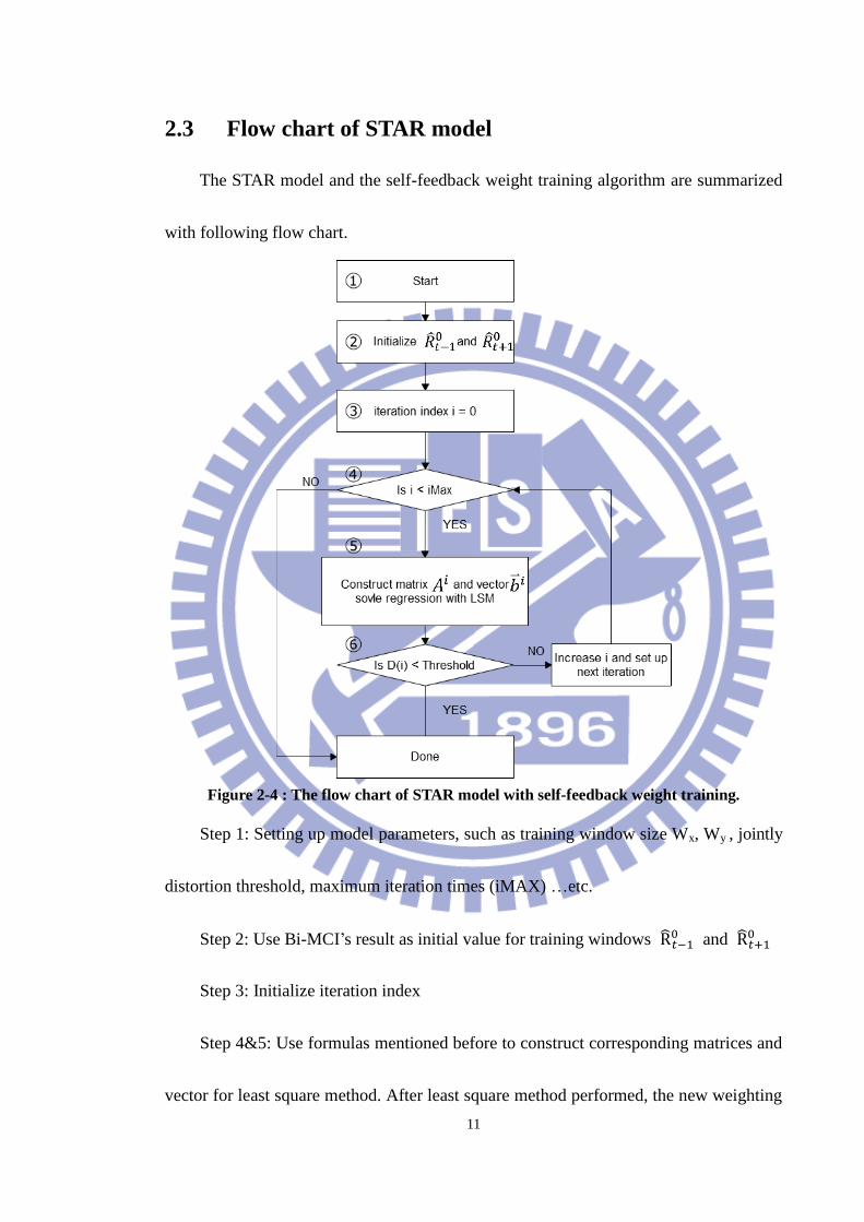
2.3 Flow chart of STAR model
The STAR model and the self-feedback weight training algorithm are summarized
with following flow chart.
Figure 2-4 : The flow chart of STAR model with self-feedback weight training.
Step 1: Setting up model parameters, such as training window size Wx, Wy , jointly
distortion threshold, maximum iteration times (iMAX) …etc.
Step 2: Use Bi-MCI’s result as initial value for training windows R̂𝑡−10 and R̂𝑡+1
0
Step 3: Initialize iteration index
Step 4&5: Use formulas mentioned before to construct corresponding matrices and
vector for least square method. After least square method performed, the new weighting

12
vector is obtained. Then the D(i) from (7) is calculated.
Step 6: Test if D(i) is less than predefined threshold or not. If it does, then the
procedure is done. Else, increase the iteration index, write back the new training
window’s result as next iteration’s initial value and loop again.

13
Chapter 3 Proposed Method
3.1 Motivation
The STAR model provides a very good visual quality for interpolated frames;
however, it also costs a heavy computation due to applying least square method.
Suppose that the support order L is set to 1 and the training window size is 32x32, each
pixel in the STAR model can be regarded as linear combination of 22 pixels. So, a
matrix A with dimension is (3*32*32, 22), needs to be constructed for LSM calculation.
The computation complexity is heavily related to the matrix’s dimension in LSM.
Besides, since time complexity of matrix inverse operation is Ο(𝑛4) , better
computation efficiency can be achieved if the matrix dimension in LSM can be reduced.
Therefore, this thesis aims at reducing the computational complexity by using a reduced
matrix dimension in LSM. Namely, fewer neighborhood pixels will be used to
interpolate the pixels. The weight analysis in STAR model [2]states that for the high
motion part in the video, pixels are strongly related to spatial neighborhood, rather than
temporal neighborhood pixels.

14
Figure 3-1 : The 2
nd to-be-interpolated frame of the test sequence Mobile_CIF. Left-top
corner marked window A with color blue, and middle-down marked window B with color
red.
Figure 3-2 : Weight distribution in window A and B of 2nd
to-be-interpolated frame of the
test sequence Mobile_CIF.
The figure 3-2 shows weight distribution for two different training windows in the
15
to-be-interpolated frame 2 of Mobile CIF sequence ( as Figure 3-1 ). The window B has
more motion intensity than window A since there is a rolling red ball across it. The
weight distribution of spatial support region in window B obviously holds large part
than those in window A. Based on the observation of weight distribution; we split the
original STAR model into two parts: temporal auto-regressive model (TAR) and spatial
auto-regressive model (SAR), and adaptively choose from one of them to perform
regression-based FRUC (ATAR and ASAR, for short). We expect that will help us
decreasing the computation complexity via reduced model and achieving better visual
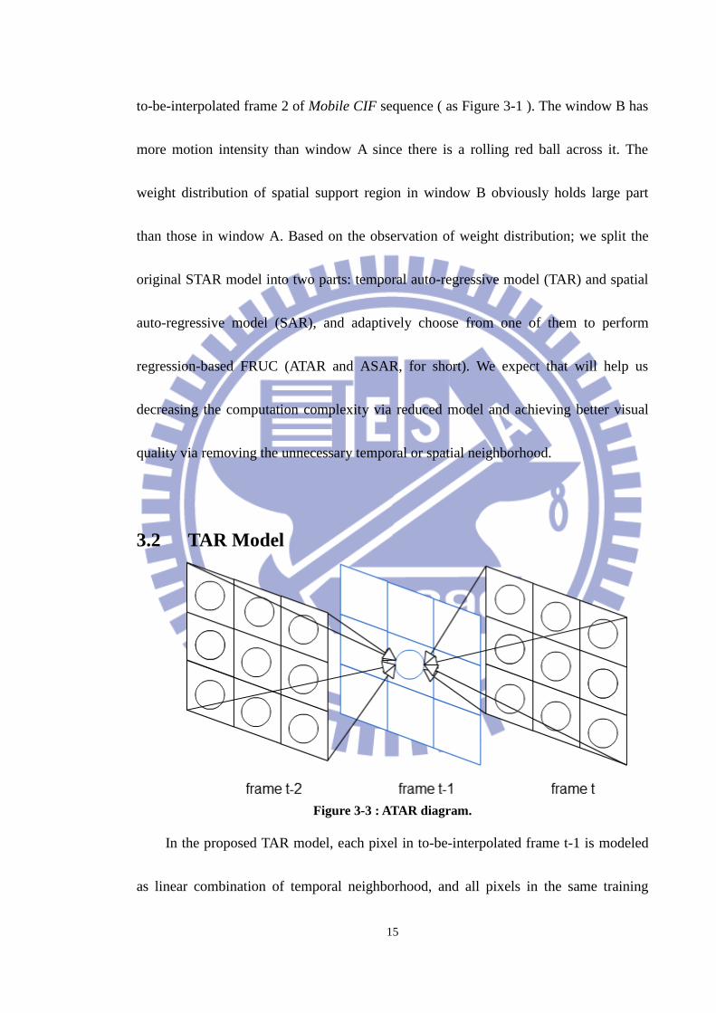
quality via removing the unnecessary temporal or spatial neighborhood.
3.2 TAR Model
Figure 3-3 : ATAR diagram.
In the proposed TAR model, each pixel in to-be-interpolated frame t-1 is modeled
as linear combination of temporal neighborhood, and all pixels in the same training

16
window will share the same weighting coefficients.
R̂t−1( k, l ) = ∑ ∑ Rt−2(k + u, l + v)
v) ≤L
× Wp(u, v)
−L≤(u,
+ ∑ ∑ Rt(k + u, l + v)
v) ≤L
× Wf(u, v)
−L≤(u,
( 10 )
The R̂t−1 means the training window in frame t-1, and Wp,Wf represents
weighting coefficients in previous temporal neighborhood and following temporal
neighborhood, respectively. The ( k, l ) represents pixel location in training window, and
(u, v) is looping index for each temporal neighborhood support region. Assuming that
support order is 1, the length of weighting vector will be 18 as illustrated in figure 3-3.
Self-feedback weight training algorithm similar to that used in STAR model is also
applied in the proposed TAR model. Since only temporal neighborhood is used, the
formula (6) is modified as follows for the approximated pixel in training window R̂t in
the proposed TAR.
R̂t( k, l ) = ∑ ∑ R̂t−1(k + u, l + v)
v) ≤L
× Wp(u, v)
−L≤(u,
+ ∑ ∑ R̂t+1(k + u, l + v)
v) ≤L
× Wf(u, v)
−L≤(u,
( 11 )

17
3.3 SAR Model
Figure 3-4 : ASAR diagram.
In the proposed SAR model, each pixel in to-be-interpolated frame t-1 is modeled
as the weighted sum of the spatial neighborhood, and all pixels in the same training
window will adopt the same weighting coefficients.
R̂t−1(k, l ) = ∑ ∑ R̂t−1(k + u, l + v)
*u=0, v=0+
× Ws(u, v)
−L≤(u,v)≤L −
( 12 )
The R̂t−1 means the training window in frame t-1, and Ws represents weighting
coefficients in spatial neighborhood. The ( k, l ) represents pixel location in training
window, and (u, v) is looping index for each spatial neighborhood. Supposed that the
support order is set to 1, the length of weighting vector will be 8 as illustrated in figure
3-4. Due to applying to self-feedback weight training algorithm, we can’t add the
co-located pixel in to-be-interpolated frame as our spatial neighborhood. Supposed that
our model contains it, then all other weighting coefficients will be zero after LSM, and
the co-located weighting coefficient will be 1.
18
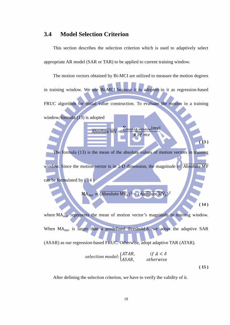
3.4 Model Selection Criterion
This section describes the selection criterion which is used to adaptively select
appropriate AR model (SAR or TAR) to be applied to current training window.
The motion vectors obtained by Bi-MCI are utilized to measure the motion degrees
in training window. We use Bi-MCI because it is adopted in it as regression-based
FRUC algorithm for initial value construction. To evaluate the motion in a training
window, formula (13) is adopted
Absolute MV̅̅ ̅̅ ̅̅ ̅̅ ̅̅ ̅̅ ̅̅ ̅̅ =∑ |𝑚𝑣|𝑚𝑣∈𝐴𝑅 𝑤𝑖𝑛𝑑𝑜𝑤
# 𝑜𝑓 𝑚𝑣
( 13 )
The formula (13) is the mean of the absolute values of motion vectors in training
window. Since the motion vector is in 2-D dimension, the magnitude of Absolute MV̅̅ ̅̅ ̅̅ ̅̅ ̅̅ ̅̅ ̅̅ ̅̅
can be formulated by ( 14 )
MA𝑚𝑣 = (Absolute MV̅̅ ̅̅ ̅̅ ̅̅ ̅̅ ̅̅ ̅̅ ̅̅𝑥)
2 + (Absolute MV̅̅ ̅̅ ̅̅ ̅̅ ̅̅ ̅̅ ̅̅ ̅̅𝑦)
2
( 14 )
where MA𝑚𝑣 represents the mean of motion vector’s magnitude in training window.
When MA𝑚𝑣 is larger than a predefined threshold δ, we adopt the adaptive SAR
(ASAR) as our regression-based FRUC. Otherwise, adopt adaptive TAR (ATAR).
𝑠𝑒𝑙𝑒𝑐𝑡𝑖𝑜𝑛 𝑚𝑜𝑑𝑒𝑙: {𝐴𝑇𝐴𝑅, 𝑖𝑓 𝛥 < 𝛿𝐴𝑆𝐴𝑅, 𝑜𝑡𝑒𝑟𝑤𝑖𝑠𝑒
( 15 )
After defining the selection criterion, we have to verify the validity of it.

19
Figure 3-5 : The validity of selection criterion of the test sequence Foreman_QCIF.
The figure 3-5 shows 𝑆𝑆𝐸𝑡−𝑠 and MA𝑚𝑣 for all the training windows in
Foreman_QCIF sequence, where the training windows are sorted in an ascending order
of MA𝑚𝑣, defined in formula (14). In figure 3-5, the left coordinate is SSEt-s’s value,
and the right coordinate is the value of MA𝑚𝑣 . Let 𝑆𝑆𝐸𝑡−𝑠 denote the difference
between TAR’s SSE and SAR’s SSE, where SSE means the sum of square error. Then,
𝑆𝑆𝐸𝑡−𝑠 can be formulated as (16)
𝑆𝑆𝐸𝑡−𝑠 = { ∑ ∑ [.Rt−1(𝑘, 𝑙) − R̂t−1𝑇𝐴𝑅(𝑘, 𝑙)/
2
+ .Rt+1(𝑘, 𝑙) − R̂t+1𝑇𝐴𝑅(𝑘, 𝑙)/
2𝑊𝑦
𝑙=0
𝑊𝑥
𝑘=0
+ .Rt(𝑘, 𝑙) − R̂t𝑇𝐴𝑅(𝑘, 𝑙)/
2
] }
− { ∑ ∑ [.Rt−1(𝑘, 𝑙) − R̂t−1𝑆𝐴𝑅(𝑘, 𝑙)/
2𝑊𝑦
𝑙=0
𝑊𝑥
𝑘=0
+ .Rt+1(𝑘, 𝑙) − R̂t+1𝑆𝐴𝑅(𝑘, 𝑙)/
2
+ .Rt(𝑘, 𝑙) − R̂t𝑆𝐴𝑅(𝑘, 𝑙)/
2
] }
( 16 )
Note that the calculation of 𝑆𝑆𝐸𝑡−𝑠 in figure 3-5 is based on available
to-be-interpolated frames, that is, the ground truth if the to-be-interpolated frame is
0
2
4
6
8
10
12
14
16
18
20
-4000
-3000
-2000
-1000
0
1000
2000
3000
4000
1
53
10
5
15
7
20
9
26
1
31
3
36
5
41
7
46
9
52
1
57
3
62
5
67
7
72
9
78
1
83
3
88
5
93
7
98
9
10
41
10
93
11
45
11
97
12
49
SSEt-s
MAmv

20
known. Rt−1, Rt, Rt+1 in formula (16) denote the ground truth of the training
windows in to-be-interpolated frames t-1, t, and t+1 respectively, while
R̂t−1𝑇𝐴𝑅 , R̂t
𝑇𝐴𝑅 , R̂t+1𝑇𝐴𝑅 represents the training window after interpolation with TAR model,
and R̂t−1𝑆𝐴𝑅 , R̂t
𝑆𝐴𝑅 , R̂t+1𝑆𝐴𝑅 represents the training window after interpolation with SAR
model. Wx , Wy are the width and height of the regression window size, and (𝑘, 𝑙) is
used to loop every pixel in the training window. Since (16) is based on known
to-be-interpolated frames, we can use 𝑆𝑆𝐸𝑡−𝑠 as an indication for AR model selection.
When 𝑆𝑆𝐸𝑡−𝑠 is smaller than zero, it means this window should perform TAR for
better visual quality. In contrast, when this value is larger than zero, it means that it is
better to apply SAR for this training window.
Figure 3-6 : The validity of selection criterion of the test sequence Mobile_CIF
The figure 3-6 is 𝑆𝑆𝐸𝑡−𝑠 vs. MA𝑚𝑣 of all the training windows in test sequence
Mobile_CIF. Since the trend of 𝑆𝑆𝐸𝑡−𝑠 is dramatically arisen around MA𝑚𝑣 = 4, we
use MA𝑚𝑣 = 4 as our selection criteria threshold.
0
2
4
6
8
10
12
14
-30000
-25000
-20000
-15000
-10000
-5000
0
5000
10000
15000
20000
15
71
13
16
92
25
28
13
37
39
34
49
50
55
61
61
76
73
72
97
85
84
18
97
95
31
00
91
06
51
12
11
17
71
23
3 SSEt-s
MAmv

21
3.5 Flow chart of proposed method
The summary of proposed method is illustrated in following flow chart. We merge
SAR and TAR with proposed model selection criterion together. δ is a predefined
model selection criteria threshold.
Figure 3-7 : Flow chart of proposed method Proposed_AST.
Step 1: Setting model parameters and use Bi-MCI’s result as initial value for
training windows.
Step 2: Calculate MA𝑚𝑣 according to formula (14)
Step 3: Judge if MA𝑚𝑣 is less than a predefined threshold δ.
If does, TAR is selected for this training window.
Otherwise, choose SAR.
Step 3: Entering AR model procedure, such as setting up LSM’s matrices and
iteration multiple times and so on.

22
Chapter 4 Experimental Results
To examine the performance of proposed method, we split various test sequences
into odd and even subsequences, perform the proposed FRUC algorithm on even ones
to generate odd ones, and evaluate the Peak signal-to-noise ratio (PSNR) of interpolated
odd frames to original odd frames. The proposed method is compared with the FA, MCI,
and STAR methods for visual quality. Also, we compared the computation efficiency
between STAR model and proposed method.
4.1 Environment
The experiment is performed on INTEL Xeon E5520 with 4GB ram. OS is
FreeBSD 8.1-RELEASE. The whole algorithm is implemented in C, with compiler gcc
4.2.1.
4.2 Model Parameters
We perform MCI with block size 8x8 and search window size 4, and implement
with quarter pixel accuracy. Full search was adopted by bi-direction motion estimation
here. The parameters for regression based FRUC, such as regression window size,
maximum iteration times, maximum support order, and jointly distortion threshold will
be listed below:
Regression window size Wx, Wy:
QCIF: 16x16
Higher resolution: 32x32

23
Maximum iteration times:
5 for STAR model
2 for proposed method
The jointly distortion threshold
50
Model selection criteria threshold (for proposed method only)
4.0
Support order
1 to 6
4.3 Objective Quality
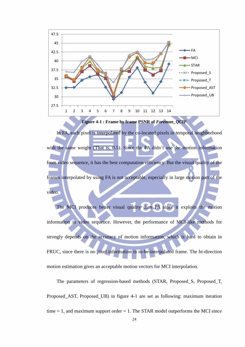
We will examine the subjective and objective visual quality in this section. The
figure 4-1 shows frame by frame PSNR of test sequence Foreman_QCIF for different
methods. Horizontal coordinate is to-be-interpolated frame index, and the vertical
coordinate is PSNR (dB). FA represents Frame Average method; MCI represents motion
compensated interpolation with bi-directional motion estimation [1] (Bi-MCI, here we
use MCI for short); and STAR represents the spatial-temporal AR model [2]. The
Proposed_S represents the proposed SAR, Proposed_T represents the proposed TAR,
and the Proposed_AST represents the method with adaptive selection between SAR and
TAR. Proposed_UB is the performance upper bound of the proposed adaptive schema
because it selects the best AR model (SAR or TAR) according to ground truth of the
to-be-interpolated frames.
24
Figure 4-1 : Frame by frame PSNR of Foreman_QCIF
In FA, each pixel is interpolated by the co-located pixels in temporal neighborhood
with the same weight (That is, 0.5). Since the FA didn’t use the motion information
from video sequence, it has the best computation efficiency. But the visual quality of the
frames interpolated by using FA is not acceptable, especially in large motion part of the
video.
The MCI produces better visual quality than FA since it exploits the motion
information in video sequence. However, the performance of MCI-like methods for
strongly depends on the accuracy of motion information, which is hard to obtain in
FRUC, since there is no pixel information in to-be-interpolated frame. The bi-direction
motion estimation gives an acceptable motion vectors for MCI interpolation.
The parameters of regression-based methods (STAR, Proposed_S, Proposed_T,
Proposed_AST, Proposed_UB) in figure 4-1 are set as following: maximum iteration
time = 1, and maximum support order = 1. The STAR model outperforms the MCI since
27.5
30
32.5
35
37.5
40
42.5
45
47.5
1 2 3 4 5 6 7 8 9 10 11 12 13 14
FA
MCI
STAR
Proposed_S
Proposed_T
Proposed_AST
Proposed_UB

25
it reduces artifacts. But regression-based FRUC such as STAR costs more
computation time than MCI does. Proposed_S (SAR), Proposed_T (TAR) and
Proposed_AST (adaptive selection between SAR and TAR) uses same model selection
criteria threshold 4. The MA𝑚𝑣 obtained from his test sequence is not significant
enough to change AR model adaptively, so Proposed_S performed almost equal to MCI,
and Proposed_T performed almost equal to Proposed_AST. The proposed_AST
outperforms the STAR model both in visual quality and computation efficiency. The
Proposed_UB represents the maximum visual quality that can be achieved under
adaptive selection. It serves as the upper bound of our proposed schema. In figure 4-1, it
is observed that the space between the Proposed_AST and Proposed_UB is quiet close,
indicating that the proposed selection criteria MA𝑚𝑣 is able to choose appropriate AR
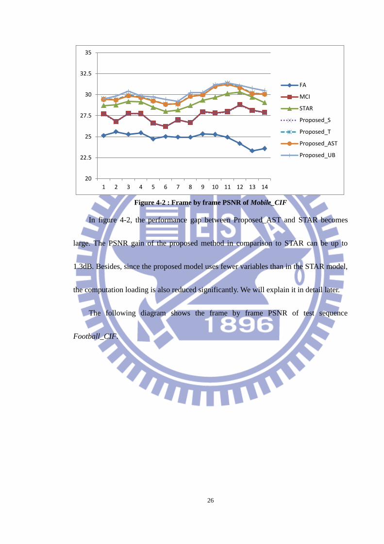
model without ground truth of the to-be-interpolated frames. The figure 4-2 shows the
frame by frame PSNR of test sequence Mobile_CIF with model parameters the same to
those used in figure 4-1.
26
Figure 4-2 : Frame by frame PSNR of Mobile_CIF
In figure 4-2, the performance gap between Proposed_AST and STAR becomes
large. The PSNR gain of the proposed method in comparison to STAR can be up to
1.3dB. Besides, since the proposed model uses fewer variables than in the STAR model,
the computation loading is also reduced significantly. We will explain it in detail later.
The following diagram shows the frame by frame PSNR of test sequence
Football_CIF.
20
22.5
25
27.5
30
32.5
35
1 2 3 4 5 6 7 8 9 10 11 12 13 14
FA
MCI
STAR
Proposed_S
Proposed_T
Proposed_AST
Proposed_UB
27
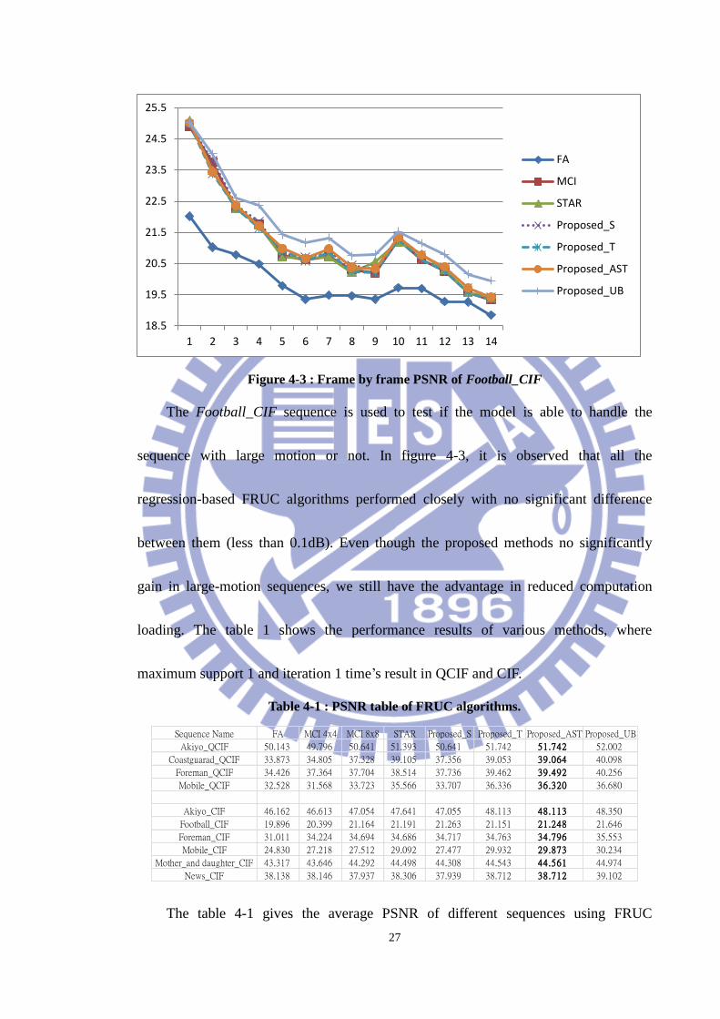
Figure 4-3 : Frame by frame PSNR of Football_CIF
The Football_CIF sequence is used to test if the model is able to handle the
sequence with large motion or not. In figure 4-3, it is observed that all the
regression-based FRUC algorithms performed closely with no significant difference
between them (less than 0.1dB). Even though the proposed methods no significantly
gain in large-motion sequences, we still have the advantage in reduced computation
loading. The table 1 shows the performance results of various methods, where
maximum support 1 and iteration 1 time’s result in QCIF and CIF.
Table 4-1 : PSNR table of FRUC algorithms.
Sequence Name FA MCI 4x4 MCI 8x8 STAR Proposed_S Proposed_T Proposed_AST Proposed_UB
Akiyo_QCIF 50.143 49.796 50.641 51.393 50.641 51.742 51.742 52.002
Coastguarad_QCIF 33.873 34.805 37.328 39.105 37.356 39.053 39.064 40.098
Foreman_QCIF 34.426 37.364 37.704 38.514 37.736 39.462 39.492 40.256
Mobile_QCIF 32.528 31.568 33.723 35.566 33.707 36.336 36.320 36.680
Akiyo_CIF 46.162 46.613 47.054 47.641 47.055 48.113 48.113 48.350
Football_CIF 19.896 20.399 21.164 21.191 21.263 21.151 21.248 21.646
Foreman_CIF 31.011 34.224 34.694 34.686 34.717 34.763 34.796 35.553
Mobile_CIF 24.830 27.218 27.512 29.092 27.477 29.932 29.873 30.234
Mother_and daughter_CIF 43.317 43.646 44.292 44.498 44.308 44.543 44.561 44.974
News_CIF 38.138 38.146 37.937 38.306 37.939 38.712 38.712 39.102
The table 4-1 gives the average PSNR of different sequences using FRUC
18.5
19.5
20.5
21.5
22.5
23.5
24.5
25.5
1 2 3 4 5 6 7 8 9 10 11 12 13 14
FA
MCI
STAR
Proposed_S
Proposed_T
Proposed_AST
Proposed_UB

28
algorithms. Compared to STAR model, the Proposed_AST have better visual quality
among all test sequences except Coastguard_QCIF. In this experiment result, the
average gain of Proposed_AST to STAR model is 0.39dB, and the maximum average
gain is 0.97dB for Foreman_QCIF. The following table shows the performance results
of AR-based methods. The maximum support order is 6 for all methods and maximum
iteration time is 5 for STAR, and 2 for proposed methods.
Table 4-2 : PSNR table of regression-based FRUC algorithms
Sequence Name STAR-IT5 Proposed_S-IT2 Proposed_T-IT2 Proposed_AST-IT2 Proposed_UB-IT2
Akiyo_QCIF 51.56663 50.6407 52.0215 52.0215 52.328
Coastguarad_QCIF 39.39581 37.3521 39.1786 39.2058 40.0316
Foreman_QCIF 39.13184 37.7581 39.6994 39.7691 40.5754
Mobile_QCIF 37.17584 33.7139 37.598 37.583 37.7705
Akiyo_CIF 47.83981 47.0545 48.1554 48.1554 48.5775
Football_CIF 21.52013 21.2864 21.2034 21.3236 22.1736
Foreman_CIF 35.11687 34.753 35.1595 35.2267 36.2934
Mobile_CIF 29.42022 27.509 29.838 29.8319 30.321
Mother_and_daughter_CIF 44.5958 44.376 44.6652 44.6787 45.0693
News_CIF 38.51697 37.9375 38.8607 38.8615 39.1862
The table 4-2 shows that even iteration times used by the proposed methods are
half of STAR model or less, the proposed methods still achieve the same or better visual
quality compared to STAR model. The average gain is 0.23dB, compared to STAR
model, and the maximum average gain is 0.63dB for Foreman_QCIF.
4.4 Subjective Quality
This section examines the subjective quality of the interpolated frame using FA,
MCI8x8, STAR and Proposed_AST.

29
Figure 4-4 : Foreman_CIF 4th
interpolated frame. (a) FA (b) MCI8x8 (c) STAR (d)
Proposed_AST
Figure 4-4 (a) is the result of FA for 4th
interpolation frame of Foreman_CIF.
Blurring happened around the ear, mouth, and helmet. Figure 4-4 (b) is MCI8x8 in the
same frame. Blurring effect is eliminated for motion compensation. Still, the artifact
around the mouth occurred because its discontinuity of adjacent block’s motion vectors.
The figure 4-4 (c) is STAR model’s interpolation result, for maximum iteration 1
and support order is 1. It alleviated the artifact around the mouth a little, and improved
overall visual quality. But it also required much computation cost than proposed method.
And a little blurring effect occurred at the edge of the helmet, since it may contain too
30
many unreliable spatial-temporal neighborhoods in moving filed. The figure 4-4 (d) is
proposed method Proposed_AST’s interpolation result. Though the artifacts around the
mouth are not totally alleviated, we improved the blurring effect at the edge of the
helmet.
4.5 Time complexity
Since we use less number of variables in the proposed AR model, the LSM’s
computation loading can be significantly reduced, comparing to STAR model. The time
complexity to compute the matrix inverse is Ο(𝑛4), where n is equal to the number of
variables in AR model. Assuming that support order is set to 1, the STAR model will
have 22 variables for LSM; while our proposed method will use only 17 variables in
average. This is because that TAR uses 18 variables, SAR uses 8 variables, and the ratio
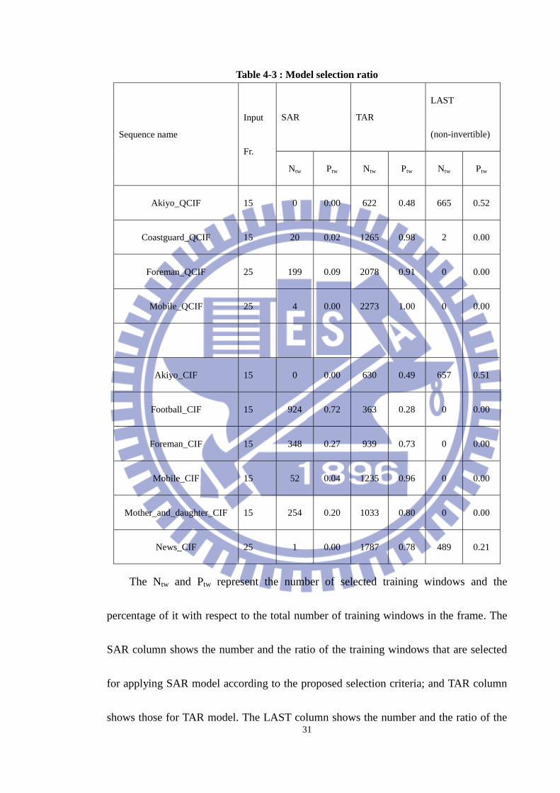
between TAR and SAR selected in our method is about 9:1. Following table shows the
ratio between TAR and SAR selected in the proposed method, where the selection
criteria threshold is set to 4.
31
Table 4-3 : Model selection ratio
Sequence name
Input
Fr.
SAR TAR
LAST
(non-invertible)
Ntw Ptw Ntw Ptw Ntw Ptw
Akiyo_QCIF 15 0 0.00 622 0.48 665 0.52
Coastguard_QCIF 15 20 0.02 1265 0.98 2 0.00
Foreman_QCIF 25 199 0.09 2078 0.91 0 0.00
Mobile_QCIF 25 4 0.00 2273 1.00 0 0.00
Akiyo_CIF 15 0 0.00 630 0.49 657 0.51
Football_CIF 15 924 0.72 363 0.28 0 0.00
Foreman_CIF 15 348 0.27 939 0.73 0 0.00
Mobile_CIF 15 52 0.04 1235 0.96 0 0.00
Mother_and_daughter_CIF 15 254 0.20 1033 0.80 0 0.00
News_CIF 25 1 0.00 1787 0.78 489 0.21
The Ntw and Ptw represent the number of selected training windows and the
percentage of it with respect to the total number of training windows in the frame. The
SAR column shows the number and the ratio of the training windows that are selected
for applying SAR model according to the proposed selection criteria; and TAR column
shows those for TAR model. The LAST column shows the number and the ratio of the

32
training windows whose constructed matrix is non-invertible AR. From Table 4-4, it is
observed that test sequences with large motion will choose SAR as their AR model,
while the sequences with low motion will choose TAR as expected.
Table 4-4 : Execution time comparison between STAR and Proposed_AST (support order
= 1)
Sequence name
STAR-IT1
(clks)
Proposed_AST-IT1 STAR-IT5
(clks)
Proposed_AST-IT2
clks ratio clks ratio
Akiyo_QCIF 369 247 0.67 1175 422 0.36
Coastguard_QCIF 473 354 0.75 2470 657 0.27
Foreman_QCIF 855 547 0.64 4416 1073 0.24
Mobile_QCIF 888 601 0.68 4339 1235 0.28
Akiyo_CIF 1677 1140 0.68 5931 1930 0.33
Football_CIF 2247 811 0.36 11896 1650 0.14
Foreman_CIF 2184 1279 0.59 11574 2560 0.22
Mobile_CIF 2240 1528 0.68 11217 2988 0.27
Mother_and_daughter_CIF 2353 1411 0.60 11300 2705 0.24
News_CIF 3556 2452 0.69 15202 4521 0.30
The above table shows the number of clocks consumed by the AR process. We
only consider the execution time for regression part of the STAR method and our
proposed method because both methods performed the same operations (MCI) before

33
starting AR model process. The support order is set to 1 in this table. The STAR-IT1,
STAR-IT5 means the STAR model is performed iteratively once and five times,
respectively. The percentages in the table show that the proposed model consume only
36% to 75% clocks compared to STAR model for iteration once. Since STAR-IT5
(iteration 5 times) and Proposed_AST-IT2 (iteration two times) have similar visual
performance, we also compare their execution times in this table and the results show
that the proposed model consume only 14% to 36% clocks, compared to STAR model.
The proposed model can save up to 86% clocks in Football_CIF, because it adaptively
chooses SAR about 72% in whole process, the average number 10.8 variables for LSM.

34
Chapter 5 Conclusion
In this thesis, an adaptive auto-regressive model for frame rate up-conversion was
proposed. In this schema for frame rate up-conversion, we save a lot of computation
loading from removing the unnecessary variables from the STAR model. In the
experimental results, we perform our proposed method compare with the other
algorithms. Also, we compare the computation efficiency with the STAR model, which
states out our proposed schema can work more efficiently and stay the same visual
quality level or even better. By seeing the upper bound in our experimental results, the
proposed model selection criteria may still have some space to be improved.

35
REFERENCE
[1] Byeong-Doo Choi, Jong-Woo Han, Chang-Su Kim, and Sung-Jea Ko,
“Motion-Compensated Frame Interpolation Using Bilateral Motion Estimation
and Adaptive Overlapped Block Motion Compensation”, Circuits and Systems for
Video Tchnology, IEEE Transactions on, April 2007, VOL. 17, NO. 4.
[2] Yongbing Zhang, Debin Zhao, Xiangyang Ji, Ronggang Wang, and Wen Gao, “A
Spatio-Temporal Auto Regressive Model for Frame Rate Upconversion”, Circuits
and Systems for Video Technology, IEEE Transactions on, September 2009, VOL.
19, NO. 9.
[3] Seok Joo Doo and Moon Gi Kang, “Generalized adaptive spatio-temporal
auto-regressive model for video sequence restoration”, Image Processing, 1999.
ICIP 99. Proceedings.
[4] Efstratiadis, S.N., Katsaggelos, A.K., “A model-based pel-recursive motion
estimation algorithm”, Acoustics, Speech, and Signal Processing, 1990.
ICASSP-90.
[5] Xiangjun Zhang, Xiaolin Wu, “Edge-Guided Perceptual Image Coding via
Adaptive Interpolation”, Multimedia and Expo, 2007 IEEE International
Conference on, July 2007 pp. 1459 - 1462
[6] Dragoljub Pokrajac, Reed L. Hoskinson and Zoran Obradovic, “Modeling

36
Spatial-Temporal Data with a Short Observation History”, Knowledge and
Information Systems, September 2003,Volume 5, Number 3, pp. 368-386