TitleOn the Particle-defining Modes for a Free Neutral Scalar Fieldin Spatially Homogeneous and Isotropic Universes(Dissertation_全文 )

Author(s) Kodama, Hideo

Citation Kyoto University (京都大学)

Issue Date 1981-03-23

URL https://doi.org/10.14989/doctor.k2503

Right

Type Thesis or Dissertation

Textversion author

Kyoto University

3 59

\'l /it El) 11 IA Z.

t th

3 59

KUNS 563

On the Particle-defining Modes for a Free Neutral Scalar Field

in Spatially Homogeneous and Isotropic Universes

Hideo KODAMA

Department of Physics, Kyoto University, Kyoto 606

Abstract

We study on the freedom in assigning Fock representations

to each cosmic time for a canonically quantized free neutral

scalar field in spatially homogeneous and isotropic universes.

Two requirements are considered: the implementability of the

Bogoliubov transformation between Fock representations at

different times, and the finiteness of the energy generation

rate per unit volume. We show that especially the second

requirement completely determines the particle-defining modes

corresponding to the Fock representations in the high frequency

region for the minimal coupling case. We also show, with no

assumption on the expansion law of the universes, that the

scalar field should interact with the background geometry

through conformal coupling in order that the Bogoliubov trans-

formation between the Hamiltonian diagonalizing Fock represen-

tations is implementable.

- 2 -

1. Introduction

In the study of canonically quantized fields in expanding

universes, we must construct Fock representations at each

cosmic time in order to give meanings to the initial states of

the quantum fields and interpret their subsequent time evolu-

tion.1)-7) These Fock representations enable us to interpret

the states of the quantum fields by particle language, and may

play important roles in various problems; the study of the

interactions of quantum fields, the statistical problems,

etc.. To find a satisfactory physical principle for the con-

struction of Fock representations in expanding universes,

however, is a difficult problem and has not been solved yet.6)'7)

In this paper we study this problem from a rather mathe-

matical standpoint and try to derive constraints in assigning

Fock representations to each cosmic time from some general

requirements. We limit our argument to the case of a free

neutral scalar field in spatially homogeneous and isotropic

universes. In this case we can expand the field by the eigen-

functions of the three dimensional Laplacian and the field

equation reduces to a decoupled system of second-order ordinary

differential equations for functions of time, fk(t), where k

denotes the eigenvalue of the Laplacian, corresponding to

momentum in Minkowsky spacetime case.2) Each selection of a

system of solutions, {fk(t)} , corresponds to one Fock

- 3 -

representation. We specify the selection at each time t=`r,

ifk('Y)(t)1, by giving the relation betweenfk and fk at t='C, as fk(T) (''C) _ (- 1 14k('Y )+Qk("( ))fk(T) (''C ), with two real quantities, Pk(t) and Yk(t)-

In order that two Fock representations can be physically

related, they must be unitary equivalent, i.e., connected by

the so-called Bogoliubov transformation.3) From this require-

ment we derive some constraints on the large-k asymptotic

behavior of )A k(t) and 4/ k(t) by examining the asymptotic

behavior of the Bogoliubov transformation coefficients. The

main point in this study is the expression of the Bogoliubov

transformation coefficients by the WKB-type expressions for

the solutions, fk(t), supplemented by the estimation of the

large-k asymptotic behavior of the correction factor to the

WKB approximation. This requirement, however, yields rather

weak constraints on ,u k(t). Thereupon, in order to obtain

stronger constraints, we next consider the energy generation

rate. Though the Hamiltonian for the quantum field in a finite

volume is a divergent quantity, the difference of its vacuum

expectation values at two differnt times, referred to as energy

generation rate in this paper, should be finite.8)'9) This is

the second requirement. From this requirement At k2(t) is

determined up to the order of 0(1) in k for large k if the

quantum field interacts with the background geometry through

minimal coupling.

- 4 -

Perhaps the most natural choice of the Fock representa-

tions is the one that diagonalizes the Hamiltonian at each

cosmic time.10),11) Some authors, however, asserted that this

choice is not adequate by showing that the Bogoliubov transfor-

mation is not implementable for some special expansion law of

the universe when the coupling is minimal.2),12)On the other

hand it was pointed out that this trouble does not occur for a

Friedmann-type universe if the coupling is conforma1.13) As a

special application of our results, we clarify this point.

Namely we show, with no assumption on the expansion law of the

universes, that the coupling of the scalar field with the

background geometry must be conformal in order that the Bogoliubov

transformation between the Hamiltonian diagonalizing Fock

representations is implementable, and for this choice the

energy generation rate also remains finite.14) Fulling has

also derived the same conclusion by a similar method to ours.17)

The program of this paper is as follows. In 4 2 we summarize

some fundamental formulas on the canonically quantized free

neutral scalar field and the Bogoliubov transformation, and

present fundamental assumptions and notations used in this

paper. In f3 we derive the expression for the Bogoliubov trans-

formation coefficients by the WKB-type solution of the wave

equation. Then in f4 we examine the large-k asymptotic behavior

of the correction factor to the WKB approximation and apply it

to the study of the constraints imposed by the implementability

condition of the Bogoliubov transformation. Next we study the

- 5 -

energy generation rate in 4/ 5. § 6 is devoted to concluding

remarks.

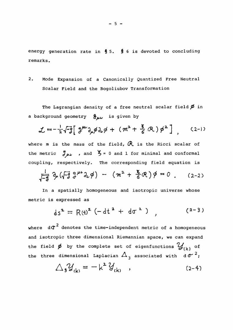
2. Mode Expansion of a Canonically Quantized Free Neutral

Scalar Field and the Bogoliubov Transformation

The Lagrangian density of a free neutral scalar field j6 in

a background geometry 3- L is given by

et _ --,', { 3.""a 56as + s c.) ~2 ] , (2.-I ) At

where m is the mass of the field, a is the Ricci scalar of

the metric ;I", , and 0 and 1 for minimal and conformal coupling, respectively. The corresponding field equation is

a7 (42-j~LaL~m+ *ck)0 . (2-2)

In a spatially homogeneous and isotropic universe whose

metric is expressed as

ds2 = R(-02 (— dt 2 + da 2 )(2- 3 )

where d Q„2 denotes the time-independent metric of a homogeneous

and isotropic three dimensional Riemannian space, we can expand

the field 0 by the complete set of eigenfunctions 24k) of the three dimensional Laplacian A.3 associated with dc3 2;

4Nek) k~~(k) 7 (2-4)

- 6 -

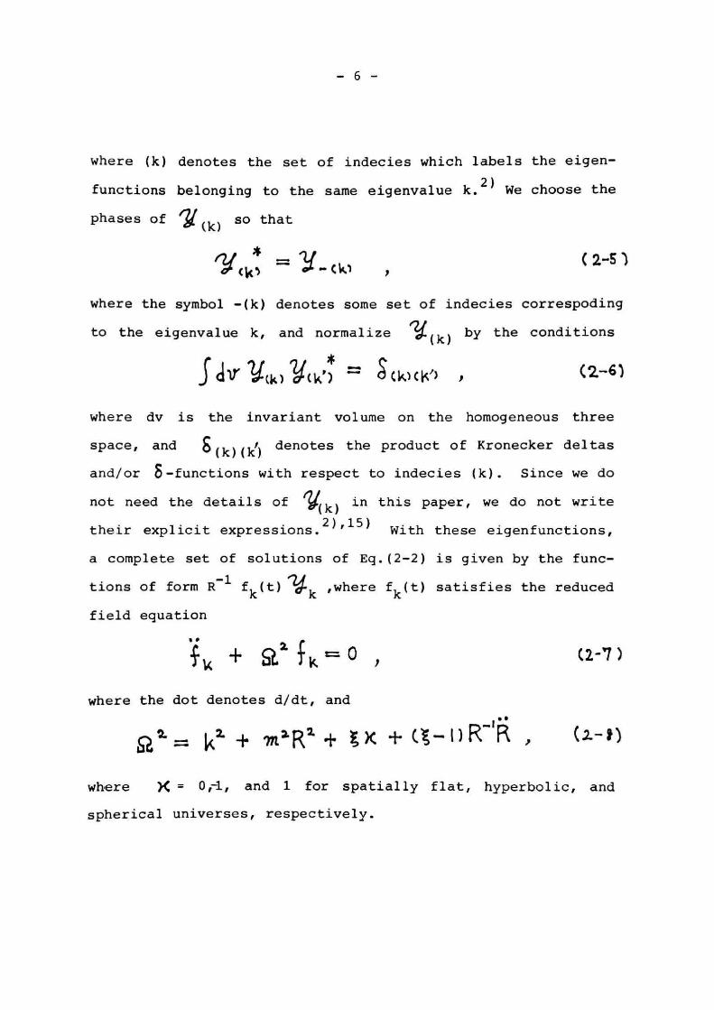
where (k) denotes the set of indecies which labels the eigen-

functions belonging to the same eigenvalue k.2) We choose the

phases of ''(k) so that

'L/* ~'(2-s d`ck).-Ck>>

where the symbol -(k) denotes some set of indecies correspoding

to the eigenvalue k, and normalize f2d(k) by the conditions

J dr ' (k) V( lc') _' S(k)( ') , (2'6) where dv is the invariant volume on the homogeneous three

space, and 8(k)(k,) denotes the product of Kronecker deltas

and/or 5-functions with respect to indecies (k). Since we do

not need the details of 1(k) in this paper, we do not write

their explicit expressions.2)'15) With these eigenfunctions,

a complete set of solutions of Eq.(2-2) is given by the func-

tions of form R-1 fk(t) 'tk ,where fk(t) satisfies the reduced

field equation

••2

k+~.f k 0 ,(2-'7 ) where the dot denotes d/dt, and

cZ2. ••••1 k1 + m2R2' + t x +(s — L ) R''R , (2- g)

where )(= 0,-1, and 1 for spatially flat, hyperbolic, and

spherical universes, respectively.

- 7 -

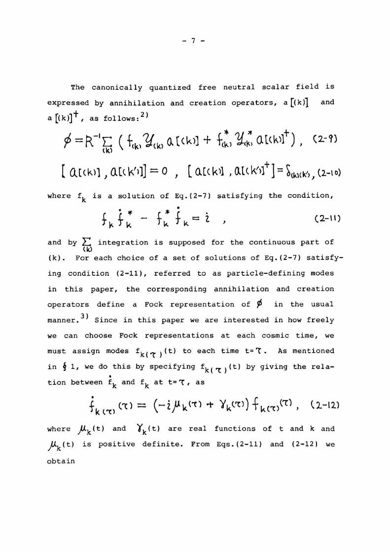
The canonically quantized free neutral scalar field is

expressed by annihilation and creation operators, a [(k)1 and

a ((k)]1- , as follows:2 )

_ R.-1E (kktk)] + 4-11 a<<k1),C2-1)

[ O [(k)] I Q[(k')]] ^ 0 , [ Q[(k)l , at( k')]+J _ s(k1(k'),(2.-to) where fk is a solution of Eq.(2-7) satisfying the condition,

ffk*—f*f kk=i I (2—t1)

and by integration is supposed for the continuous part of (k)

(k). For each choice of a set of solutions of Eq.(2-7) satisfy-

ing condition (2-11), referred to as particle-defining modes

in this paper, the corresponding annihilation and creation

operators define a Fock representation of 0 in the usual

manner.3) Since in this paper we are interested in how freely

we can choose Fock representations at each cosmic time, we

must assign modes fk(' )(t) to each time t='Z. As mentioned

in § 1, we do this by specifying fk(1)(t) by giving the rela-

tion between fk and fk at t='(, as

(ex ) ..—_—_. (— ifi 01)-1..Y(`L)1r (T)

where )dk(t) and Ik(t) are real functions of t and k and

IUk(t) is positive definite. From Eqs.(2-11) and (2-12) we

obtain

- 8 -

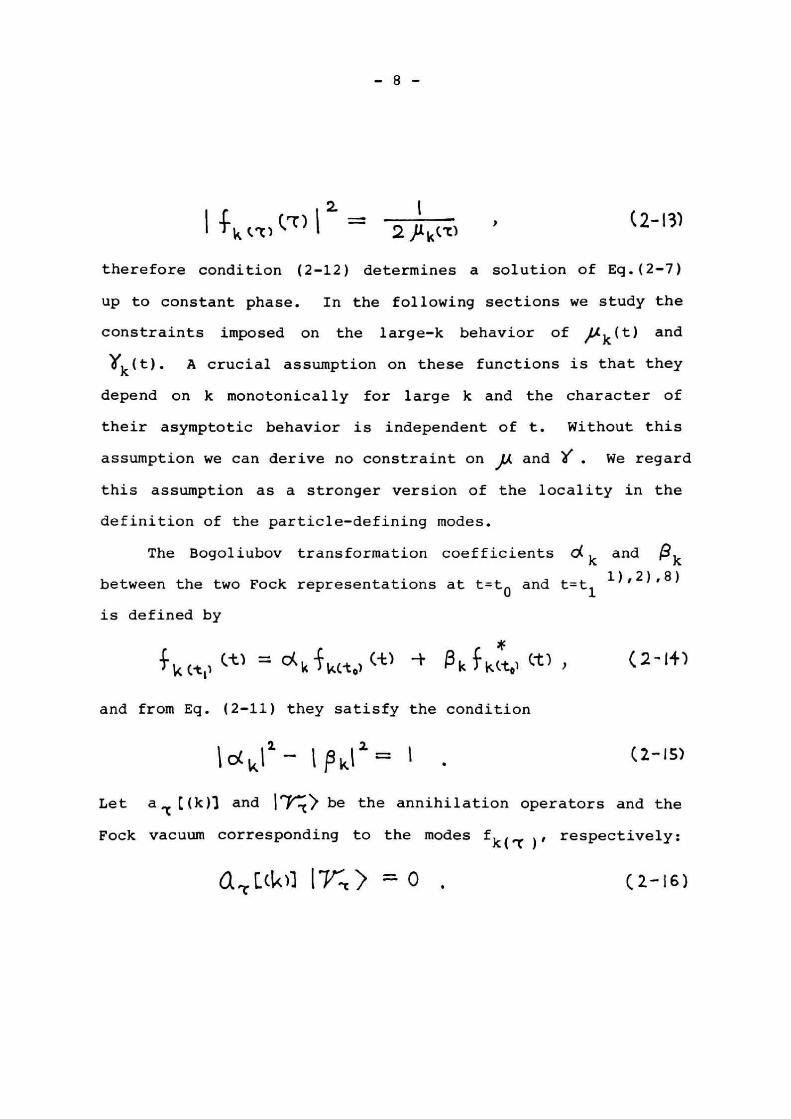
Ifk('r) t2 2)1k (2-13)

therefore condition (2-12) determines a solution of Eq.(2-7)

up to constant phase. In the following sections we study the

constraints imposed on the large-k behavior of Pk(t) and

1°'k(t). A crucial assumption on these functions is that they

depend on k monotonically for large k and the character of

their asymptotic behavior is independent of t. Without this

assumption we can derive no constraint on )A and Y. We regard

this assumption as a stronger version of the locality in the

definition of the particle-defining modes.

The Bogoliubov transformation coefficients d k and (3k

between the two Fock representations at t=t0and t=t11),2),8)

is defined by

LL

k ct, (t) = 6' k i k(t,d(+) -+ R kTk(t,i (t)) (2-14)

and from Eq. (2-11) they satisfy the condition

10(0- t kt I •(2-IS)

Let a1[ (k)'] and IT-) be the annihilation operators and the

Fock vacuum corresponding to the modes fk(„r), respectively:

a [(14 VVC) = 0 .(2-16)

- 9 -

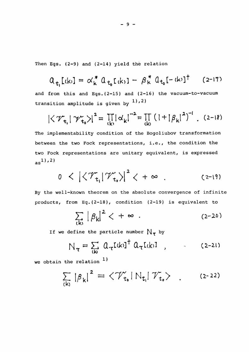
Then Eqs. (2-9) and (2-14) yield the relation

Qt C(k)1 = O( atot(k))/31,ato[--(k)]t (2-17)

and from this and Eqs.(2-15) and (2-16) the vacuum-to-vacuum

transition amplitude is given by1),2)

I<7'ti'>~27~kll1flk12) • (—) (k)(k)

The implementability condition of the Bogoliubov transformation

between the two Fock representations, i.e., the condition the

two Fock representations are unitary equivalent, is expressed

as1),2)

0<1<rl`- 0>12<+ (2-0) By the well-known theorem on the absolute convergence of infinite

products, from Eq.(2-18), condition (2-19) is equivalent to

E lPkI Z < °° •(2-20) (k)

If we define the particle number NT by

N.~ = EQzt(ke Q,t(k)] , (2.-2.t) do

we obtain the relation1)

z

E IPkI = <7 to I N.,l vo> (2.— 22) (k)

- 10 -

The right-hand side of Eq.(2-22) represents the number of the

particles generated at t=t1 from the vacuum state at t=t0,

therefore it is, if not zero, infinite for the open universes.

This is a familiar trouble associated with the infinite spatial

volume and not physically essential one. We avoid this difficul-

ty in the usual manner1)by restricting the field in a large

but finite volume, and imposing some appropriate boundary

condition on it. Then, noting that the equations which determine

g k, Eqs.(2-7),(2-12) and (2-14), are all independent of the structure of the spectrum of k, hence so is 1 k itself, and

that the number density of modes with respect to k per unit

volume is proportional to k2 for large k regardless of K ,

the implementabitity condition of the Bogoliubov transformation

can by expressed instead of Eq.(2-20) as

-r

J°°k I k I k 1 K -t- 00(2-Z3) Here we assumed that there occurs no infrared trouble since we

are working in a finite volume.

3. Some Formulas for the Bogoliubov Transformation Coefficients.

In this section we derive formulas which express the

Bogoliubov transformation coefficients by the correction factor

to the WKB approximation for a solution of Eq.(2-7). These

formulas play important roles in the study of the large-k

- 11 -

asymptotic behavior of 0/ k and i k , and the constraints imposed

on A and Y in the following sections.

Let X(t) be the solution of Eq.(2-7) satisfying the condi-

tion

where a() is the value of a at t=t0 . Then f (to(t) (j=0,1)

are expressed by X(t) as

S. (t = A.X + B} X* (3-2)

From now on the subscript k for various quantities will be

suppressed. From conditions (2-12) and (2-13), we can express

Aj and Bj by X as

i9 er •

2o[X1-(i~l;—Y•)X]C 3-3) Y~r"

_ -------- [ X~+(.p~—~'a.) Xd.1,( 3-4) 2,SZo

where the subscript j for the quantities in the right-hand

sides represents the values estimated at t=tj, and ej are

arbitrary real numbers. From Eq.(2-14) cy and (9 are expressed

by Aj and B, hence by X as

*i C6^—eo) o(=2sz0CA°Ai—BBil= -----------(3—s)

- 12 -

R ((~~Aez(eo*s,~ 2&°oS1Bo~'1I--

where

-6 =- ('—t ipo _ yo) CXI* t Cip1—Y1)X1*

CZ$Z6.. ipo— Yo ) C5(1 + Up, _Y1)XI ] ,

et = (—Zaa+ Z(j0Y ) [X1r + (2)A1-11)"*J + ip0-- ) L X1 fi (tilt - YI) X1) .

Now we introduce the following WKB-type expression

X(t)

fa: 4 6? Gett)

where t

(t) C8 Ct') S~ (t') eft' to

The correction factor dB (t) to the WKB approximation is

solution of the differential equation

ci265t(A.+l-03-4)C8 =o ;~(t°)=l,d~CJ=4, d4

where

t

4 ; =4 51(t')dt' , to

and

1 lda2 1ldig?.=4s~;~d;~r2si d2

(3-6)

(3-7)

(3-8)

for

(3-1)

(3-I0)

the

(3-11)

(3-12)

- 13 -

[(1 2,).I2 1 (Se)" 166s`} a4 (3-13)

We can prove that the solution 65(t) of Eq.(3-11) exists in

the whole range of 4 if 64)o ,thereforethe expression (3-9)

is valid in the whole range of t. But since its proof is

lengthy and of highly mathematical nature, and since Eq.(3-11)

has been fully studied in the context of the WKB approxima-

tion by many authors16), we admit this fact without proof in

this paper. By substituting the expression (3-9) into Eqs.(3-7)

and (3-8) we obtain the final expressions:

'6 =C811, t' I slat + 62. cos/1 + i (`Cs3 sin/, + 64 cos/ ,), (3-14) = a31a [zini 1. of COS §.1 Z Gt3 Sin~, 1.44c0311)], (3-IS)

where B1 =05(t1), 'Q1 =,Q(t1), and gE1 =I(t1), and

„Si -' }Lvyl) t)11 ga.•t2~oL8~(3-1c)

(4%.= 2( µ12Q- )10 a-z)(3-\'T)

oat 3` 2 (5Lo341 4131 2^)Aof t ) + 2 Ve u2, }~0.~, tYL~c + Yoy1 — CA1.0_ -r 2 io)(3-4)

tt4.=- '20-2;—SZ, a5' 2+ 2CSigoY1 - Yo~1~i —25a075711 (3-11)

- 14 -

and the expressions for 6 (1=1.'4) are obtained by the re-

placement 1/0-1,-)A0 in those for ofl1 .

4. Constraints Imposed by the Implementability Condition of

the Bogoliubov Transformation.

Now in this section we study the asymptotic behavior

of QJ for large k and from this we derive constraints on

j.4 and )1 imposed by the implementability condition of the Bogoliubov transformation. Since in the usual WKB approximation

as ; 1, we change the variable from 413 to u =d9-1. Then Eq.(3-11)

is written as

1

d+ 4 u = ( I + u) /~,. -- (A (u)(4-0 where

(U)._U1~3 U'-~-8ut6)(4-2) Ct+U)E

and the initial condition is

LA(so=0 ducro=0(4-3) With the aid of the Green's function of the differential opera-

tor d2/d 524 4, Eq.(4-1) can be transformed to the integral

equation

UIC~)=—isin ;--1C') [(1+u()) AZ) t a(Lt('))1dt' (4-4)

- 15 -

Returning to the original time variable t, we obtain

t t

(J (t) = -i1 sin (2 .,a Ct'~~dt'') [( ituct')ASV) t uct') %(uct")l,(t5dt t.t

(4-5) and

u(t) = - SZ(t)tCO3(2JtS~.ct•>dt") [(I-t u(t')) Act') -t- uct').(uct'))] 6? t')cft' ~ t. t'(4-6)

Now we will derive the estimations of u(t) and u (t)

by A. (t) from Egs.(4-5) and (4-6). Let A (t) be the maximum

value of lu(t')1 for to 6 t'i t ,and tx be the maximum value of t,

such that

rt

.,Jt~(u(t')) 1 61(t')(it' < I(4-'7) and

t

it A(t') l a(t')dt' <-12-..(4-8) to

Then from Eq.(4-5), we obtain the inequality for to t S tip

t

I tut) I <i(1 + AM)).t.i AW)ISZ(t') dt'-t- 4A(). (4—i) Since the right-hand side of Eq.(4-9) is a monotonically increas-

ing function of t, we can replace (u(t)I by A(t) in this

equation. By solving it with respect to (t), we obtain for

to 6 t s t,p, t

A(t)62J I A(t'012,(t') dt' .(4-10 to

is

- 16 -

Here suppose that t* remained finite as lA(t)I a (t) and

LA(t)1611(t)2 converge to zero locally uniformly. Then from

Eq.(4-10) and the definition of g(u), the left-hand sides of

Eqs. (4-7) and (4-8) both tend to zero even for t=t*, leading

to the contradiction to the definition of t*. Therefore, for

any t1 (>t0), Eq. (4-10) is valid in tOst‘ti if 1/A(t)1SZ(t)

and l/Ut)l .(t)2 is sufficiently small uniformly in this

range. Thus we obtain the estimate

IU(t)I < 2 Jt IAC-t')I 2(t') dt' , (4-11) to

which is valid for any t()' t0) under the same condition. A

similar estimate for u(t) can be obtained from this. Using

conditions (4-7) and (4-8), and noting that lu(t)141 from

Eq.(4-11) under these conditions, Eq.(4-6) yields the estimate

t

Iuct)Is 42(t)j A (t') I SZ(t) cl t' . (4-12) to

If gi exists, we can obtain finer estimations. By partial

integration Egs.(4-5) and (4-6) are written as

t uIt) =-4[/1c±)(it tut))+u(t)9(U(t))]---4-4tcos(2fSZ(t'dt') t ±cos2it2(elAt•),[n(l+u)+Ow]dt;

' andt(4-13)

u(t)_—2bZ(t) Act)sin(2 çtF)at/)

- 17 -

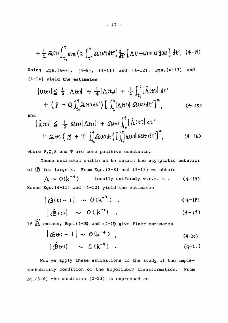
tt -t'1s(to Jsin(zJ,S2,(t'')dt"), r.A(l+L&)+u ltu)~dt'.(4-14) t,t

Using Eqs.(4-7), (4-8), (4-11) and (4-12), Eqs.(4-13) and

(4-14) yield the estimates

RA(*) IzIA.(t)I -I-"TIAdo)( *zlt otln.(t'>Iit' t(p+Q S.(tl)dt') [ 1tjA.tt')I 9ct'~dt-1Z,t,

and

(act)!!sz(~)I/~c~~(+ac-t)~*IA.(t')I dt' Zto

+ 9,4) (S + "C StS~(t5dt')tlIltt')l~2.(t')d-t'11,(4- IC) t,t.

where P,Q,S and T are some positive constants.

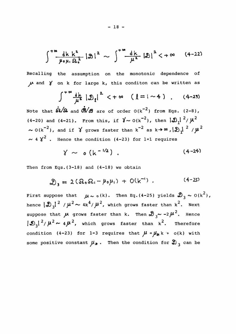
These estimates enable us to obtain the asymptotic behavior

of ® for large k. From Egs.(2-8) and (3-13) we obtain

0(k-4)locally uniformly w.r.t. t .(4- 17)

Hence Egs.(4-11) and (4-12) yield the estimates

143(t) -- c I 0 (k-3 ) ,(4^Ip)

0(k 2) .(4— I) ...

If a exists, Eqs. (4-15) and (4-16) give finer estimates

og(t) - I I --- 0 (k-4 ) ,(4-20)

Owl - 0(k-3) .(4-al )

Now we apply these estimations to the study of the imple-

mentability condition of the Bogoliubov transformation. From

Eq.(3-6) the condition (2-23) is expressed as

- 18 -

I' be

d--------------koksZ ^~12.(dxt4-221

''<~ftla

Recalling the assumption on the monotonic dependence of

JtA and ' on k for large k, this conditon can be written as

rt.2 Note that 62/St and (W are of order 0(k-2) from Eqs. (2-8) ,

(4-20) and (4-21). From this, if Y^- o(k-2), then 1.011 2/)A2

...-0(k-2), and ifYgrows faster than k-2 as k-..)oo,1JJ 112 /2

4 .2 . Hence the condition (4-23) for 1=1 requires

o ( k - I/2)(4 -24)

Then from Eqs.(3-18) and (4-18) we obtain

cat3 . (SLR! -- Foy') + o(k-I) . (4-2s)

First suppose that At.., 0(k). Then Eq.(4-25) yields 01D3 0(k2),

hence12/1A2,_k42,which grows faster than k2. Next

suppose that IA grows faster than k. Then 015r, -442. Hence

11)312012,, 4/A2, which grows faster than k2. Therefore condition (4-23) for 1=3 requires that 1.1 =/11k +o(k) with

some positive constant p,,. Then the condition for 2)3 can be

- 19 -

written as

I°253 Io (k-4) .(4-16)

By rewriting the first term in Eq.(4-25) as

a s

and noting that the last term in this equation is of order

0(1), we can easily see that condition (4-26) requires

t

ill=,~_ 4o(k2)( 4— 2.7)

With Eqs.(4-24) and (4-27), all the conditions (4-23) are

satisfied, and these are the constraints we wanted to obtain.

In concluding this section we remark on a special case.

Among various choices of the particle-defining modes, that

which diagonalizes the Hamiltonian at each cosmic time is the

most natural one. For this choice we can derive an interesting

fact from the result obtained in this section. As will be

shown in the next section, for the Hamiltonian diagonalizing

modes, y=0.-1,R R. Then condition (4-24) requires that -1'-1'

t =1 unless RO RD and R1 R1 are both zero. Therefore we can

conclude that the coupling of a scalar field with the background

geometry must be conformal in order that the Bogoliubov trans-

formation between two Fock representations at different times

specified by the simultaneous Hamiltonian diagonalization

condition is implementable.

- 20 -

5. Constraints Imposed by the Energy Generation Rate

The constraints on p and Y obtained in 1 4 from the

implementability condition of the Bogoliubov transformation

are rather weak ones in general. In this section we show that

stronger constraints are obtained if we turn our attention to

the energy generation rate. For the scalar field in a spatially

homogeneous and isotropic universe we define the Hamiltonian

by

N ('t) = -- R4(1) S ay. t(5-1) t=T

where T', are the mixed components of the energy-momentum

tensor. Then the difference of the vacuum expectation values

of H(t1)at t=t0and t1 ,

A 6 -.. <ert, 1 H (-t 0 I 7- — <7;11H (t017-;,> , which is referred to as energy generation rate in this paper,

should be finite if we restrict the field in a finite volume,

though H itself is a divergent quantity.8)'9) This is the

second requirement, which we consider in this section.

The energy-momentum tensor of a scalar field A in a

background geometry go, is given by8)

T„,,,=--2Ji4xL

- 21 -

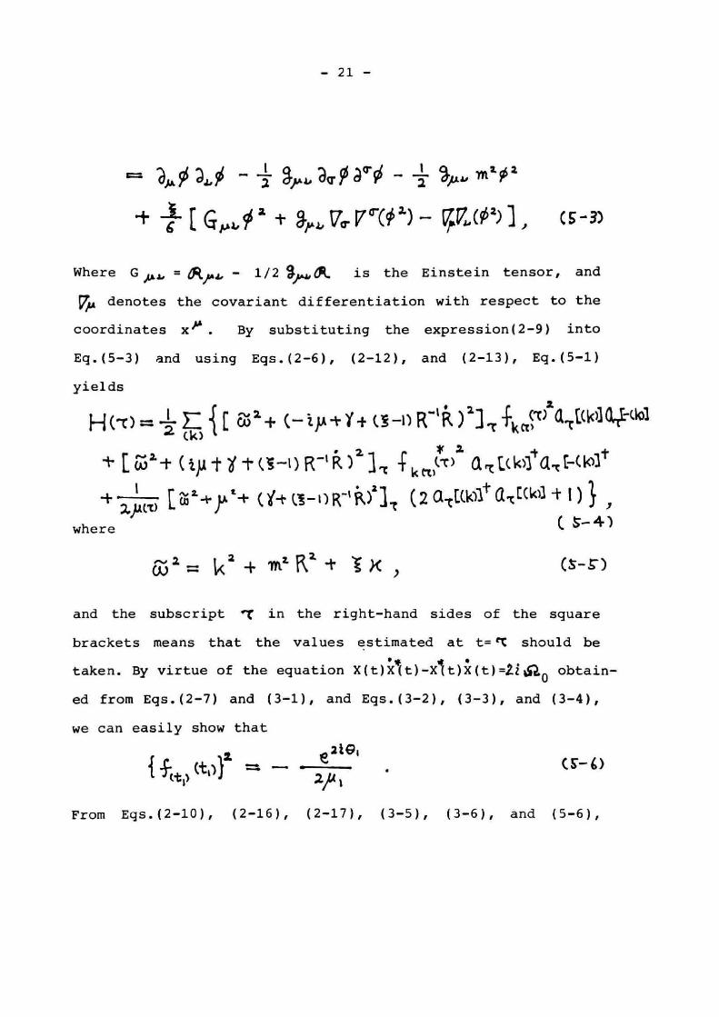
= a/+^FS aL _ 1 aju^i, 493 a°rsi - Z ,uy mxe

• 1.- C G ,uL 91 a + a'pti, VIcr r(56 Z) -- Vag, (952) ](S. - 3)

Where GA,, = ffitps, - 1/2 gf,,,,cR, is the Einstein tensor, and

PI denotes the covariant differentiation with respect to the

coordinates x 4. By substituting the expression(2-9) into

Eq.(5-3) and using Eqs.(2-6), (2-12), and (2-13), Eq.(5-1)

yields

H ('t) = ziai E C' + (-11.A* Y + cg -1) R-' R )1]T4icciv all(k)14-(b) (k)

+ ['.-- (41t t(I-1)R-'R)21rr f kn,c-c) artt(k)ata.t[-(k'at + 'z'c_)[ ~Z-~ ys+ (Y-t «- ) R-1 k)=].~ (2 a-c[ckea.k)]+I)},

where c 5-4)

W2 = k2-* 1 X)(S-5)

and the subscript ''t in the right-hand sides of the square

brackets means that the values estimated at t=e( should be

taken. By virtue of the equation X(t)X(t)-X1 t)X(t)=21al0 obtain-

ed from Eqs.(2-7) and (3-1), and Eqs.(3-2), (3-3), and (3-4),

we can easily show that

{Z(S-6) 2/,

From Egs.(2-10), (2-16), (2-17), (3-5), (3-6), and (5-6),

- 22 -

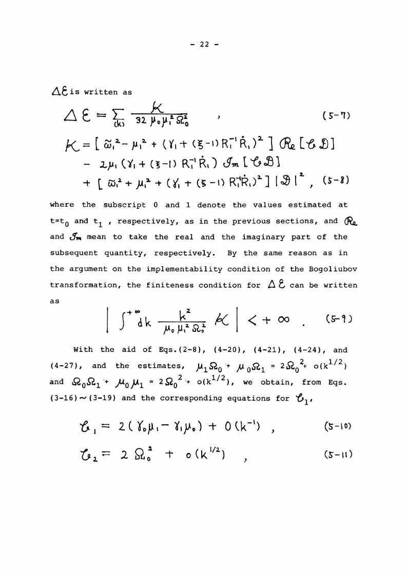
aG is written as

E =_- Ez(s-1) (to 32120

K= [ w,Z—,2 + (Y,-t- c ,-1)R;'R,)2 ] 0?„e. C-&,,B] — (Y1+ (t—t) R;`Rt) drift L`e.90

-t-[U,?1+ +)1,-(Y~-t-(;-t)R;R,)2] I IL, (5-8)

where the subscript 0 and 1 denote the values estimated at

t=t0 and t1 , respectively, as in the previous sections, and

and J,,mean to take the real and the imaginary part of the

subsequent quantity, respectively. By the same reason as in

the argument on the implementability condition of the Bogoliubov

transformation, the finiteness condition for LE can be written

as

Jak ----------~&(5-9) po µ‘o

With the aid of Eqs.(2-8), (4-20), (4-21), (4-24), and

(4-27), and the estimates, p1,~0+/u0n1 = 2,~,02+ o(k1/2)

and `Q0a1 + )(lop] . 26202 + o(k1/2), we obtain, from Eqs. (3-16)--,(3-19) and the corresponding equations for /51,

t , = z ('oµ, — o (k-') ,0.- t 0)

ritz -i- o (kvz)(s—tt)

- 23 -

6 3 = 2 ut p2 + C (k'_)(s- 11)

64 = 2 (Ro?l - 6 Y.) * 0 (k"%) ,(s-o)

and

et, a 2 (roy,+ Yip 0) + pia igto+y,SZ, IA,+ O(k=),(5-14)

.is = 2 (Slept -atilt)* 0 ( k-2) ,(s-1s)

Zs= 2. (2094- Pop') -I. 0 (k-u) ,(s-i 6)

1: 2(2°11-1°60+ a•RAT'-u2iSao'sto+o(k-') , (s-r1)

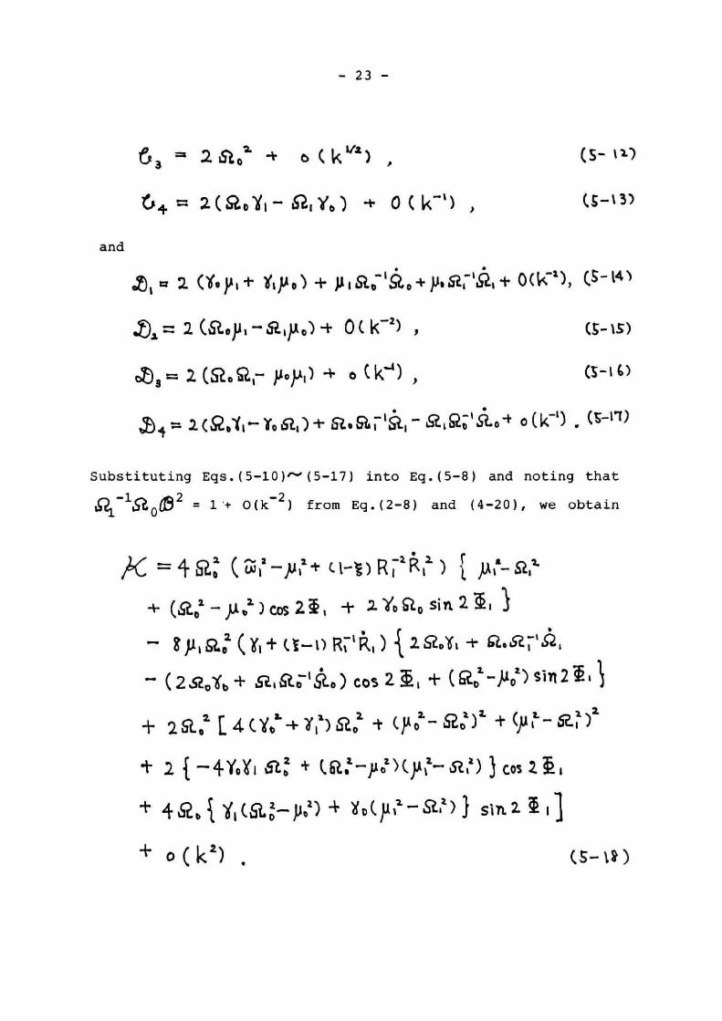
Substituting Egs.(5-10)^•"(5-17) into Eq.(5-8) and noting that

-161O02 = 1'+ O(k-2) from Eq.(2-8) and (4-20), we obtain

hC ;4SZ Calla—pill. (1-t)R-aR11) 1 p,-a% + (u2.o -)1 ) cos 21, + 2. YD SZo sin 2 II

-- s p, ao (U, + U-- t) R; ' R,) { 2 sza, -+- k• sa; ' h i yy[[~~(''' — (Zs<'pOp + ~117Lp1~71-0~cos2 L + `~0-#01) Sin 2 L,

+ 2SL, [4(Yo -t'/Il)SZo -t' (yo -SZc)Z +9.1j'-62. )_

t 2 { —4Y0X1 6 + (ba: —po)()A _ s?.) 3 cos 2 L

+ 45Z6 si,(SZD-po) 4 mil -sZ?) } sin2 1 I1 + 0 (k2) .(s- a)

- 24 -

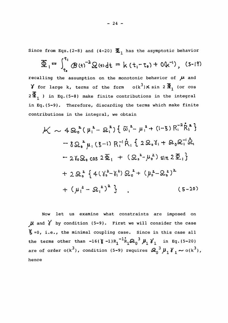
Since from Eqs.(2-8) and (4-20) 1E1 has the asymptotic behavior

t,

t03(t)-2. (-0 dt^04c-'),(5-17) to

recalling the assumption on the monotonic behavior of )A and

for large k, terms of the form o(k3)X sin 2 !i1 (or cos

2 1 ) in Eq.(5-8) make finite contributions in the integral

in Eq.(5-9). Therefore, discarding the terms which make finite

contributions in the integral, we obtain

K 4 SIo C1~,Z-SZ~'){w,t-P,Z -t. (t—U R t.--8 2:11 , U—t) R^'R,2SZoif, -t5.0a,'R.,

2 Yo SZ,o cos 2 , + C SZoa-,o) sin 2 11 }

2.12.01 { 4 CV--)'12) Roz+ (p L-0 )2-

-~. (P i25~ .,2 )z(5-20)

Now let us examine what constraints are imposed on

J(i( and 0 by condition (5-9). First we will consider the case

=0, i.e., the minimal coupling case. Since in this case all

the terms other than -16(V -1) R1 R1`c.0 )1'1 in Eq. (5-20 )

are of order o(k3), condition (5-9) requires 6203P1 Y 1 o(k3)I

hence

- 25 -

Y o (k-')(5-21)

Furthermore in order that the contribution from the oscillatory

terms is finite, it should be that 5102 JlL 1( g02 JA 02) .., 0(k3).

hence

Ra2 -F o ( )C5-22)

Under the conditions (5-21) and (5-22), condition (5-9) is

equivalent to the condition Et02 Ai1(20.0y1+sl 0`Q1-1`21)

o(k2), hence

= -!SC'S? , -+o(k-2).CS -2-3)

2 Next we consider the case 1=1, i.e., the conformal coupling

case. In this case, Eq.(5-20) reduces to

K 2 wo { (µo -- w 01)1 - (y?- w17-)2. -t 41742(g (5-24) Therefore condition (5-9) is equivalent to the condition

..616 [ )), ) 4 crol xi] where 21 means to take the difference of the values estimated

at two different times. In summary, for the minimal coupling

case, the requirement that the energy generation rate is finite

yields very strong constraints on At and y and they are com-

pletely determined by in large-k region in essence. In

contrast, for the conformal coupling case, only a rather weak

constraint (5-25) is imposed.

- 26 -

Finally we will remark on the special case in which the

particle-defining modes are specified by the simultaneous

Hamiltonian diagonalization condition. From Eq.(5-3) this

case is characterized by

N

)A -- cY=(I-s) IV‘ R . (5-2C)

In this case, as was shown in §4, the implementability condi-

tion of the Bogoliubov transformation requires that g =1.

Therefore condition (5-25) is satisfied. Since for the Hamil-

tonian diagonalizing modes, the normal-ordered Hamiltonian

with respect to these modes at each time is always finite and

positive definite, Q f can be said to mean the energy genera-

tion rate on its proper sense. Hence we can say that for the

Hamiltonian diagonalizing Fock representations and the conformal

coupling, the energy generation rate remains finite as well as

the Bogoliubov transformation is implementable.

6. Concluding Remarks

•

In this paper we studied on the freedom in assigning Fock

representations to each cosmic time for a free neutral scalar

field in spatialy homogeneous and isotropic universes. We made

this assignment by specifying the particle-defining modes at

each time with the aid of two functions, pk(t) and Yk(t). In

- 27 -

order to obtain constrains on Pk(t) and Yk(t), we considered

two requirements. The first of them, the implementability

condition of the Bogoliubov transformation imposed rather weak

constraints, but the second requirement that the energy genera-

tion rate per unit volume should be finite yielded strong

constraints on the large-k asymptotic behavior of , k(t) and

'Yk(t. Especially for the minimal coupling case, /4 k(t)

and Yk(t) were, in essence, completely determined by the mode

frequency SZ(t) in the large-k region.

Here we comment on the work of Fulling.17) He examined

whether the unitarity condition (2-23) is satisfied or not

for modes suggested by the first-order WKB approximation for

the field equation in the generalized Kasner universe. When

restricted to the isotropic case, the modes he examined in

detail correspond to those given by =52, and Y= 0 in our

notation. Of course he also dealt with some more general

cases in connection with the canonical Hamiltonian diagonalizing

modes, but in these cases his consideration remained rather

rough one. By using our results his conclusion on these cases

can be also justified exactly. Next we refer to technical

aspects. Since his argument was based on the estimation of

the direct difference of the WKB approximation from the exact

solution, it was difficult to obtain the information on the

phase of the error. In contrast, in our method, since we

confined the correction for the WKB approximation to a single

- 28 -

real function G5, we could explicitly distinguish the correction

to the amplitude from that to the phase, which enabled us to

obtain the delicate constraints on A and Y

In general our consideration does not give informations

on the small-k behavior of ,t4k(t) and Yk(t). In order to

determine AU k(t) and Yk(t) in the full range of k, more deeper

physical considerations should be needed. But in the cases

where the particle defining modes are determined by other

physical grounds, our results give an important criterion on

their acceptability. In fact, especially for the simultaneous

Hamiltonian diagonalizing modes, we showed that the coupling

of a free neutral scalar field with the background geometry

should be conformal in order that the Bogoliubov transformation

between Fock representations at different times is implementable.

Since, for the high frequency modes, the assumption on the

locality of the definition of the particle-defining modes

might be reasonable, and the positive definiteness of the

Hamiltonian might be also required, physically acceptable Fock

representations will diagonalize the Hamiltonian in the large-k

region. Therefore, the fact stated above seem to suggest that

scalar fields should interact with the background geometry

through conformal coupling.

Finally we remark on the extent to which our consideration

is valid. Our consideration crucially depend on the quasi-

adiabatic nature of the definition of particle modes and the

- 29 -

validity of the WKB-type expression (3-9). Especially near

the cosmic singlarity these assumptions may break down. In

such a region non-local characterization of field states may be

necessary_ Assumption on the isotropy of universes also seems

to have played an important role. In fact Fulling has shown

that anisotropy brings in a new serious difficulty to the

consideration of the unitatity condition.17) These problems

remain to be solved in the future.

Acknowledgements

The author would like to thank Professor C. Hayashi and Professor

H. Sato for their continuous encouragements.

References

1) L. Parker, Phys. Rev- 183 (1969) 1057.

2) L. Parker, and S.A. Fulling, Phys. Rev. D9 (1974) 341.

3) L. Parker, in Asymptotic Structure of Spacetime, edited

by F.P. Esposito and L. Witten (Plenum Press, N.Y. and

London, 1977),

G.W. Gibbons, in General Relativity — An Einstein centena-

ry survey, edited by S.W. Hawking and W. Israel (Cambridge

University Press, 1979).

4) G.W. Gibbons and S.W. Hawking, Phys. Rev. D15 (1977)2738.

5) C.M. Chitre and J.B. Hartle, Phys. Rev. D16 (1977) 251.

6) M.Castagnino and R.Weder, Phys. Let. 89B (1979) 160.

7)

8)

9)

10)

11)

12)

13)

14)

15)

16)

17)

- 30 -

H. Nariai and T. Azuma, Prog. Theor.Phys. 64 (1980)

No.4, in press.

B.S.Dewitt, Phys.Rep. C19 (1975) 295.

R.M. Wald, Comm. Math. Phys. 54 (1977) 1;

Ann.Phys. 110 (1978) 472.

G. Labonte and A.Z. Capri, Nuovo Cimento 10B (1972)583.

A.A. Grib and S.G. Mamayev, Sov.J. Nucl. Phys. 10

(1970) 6; 14 (1972) 450

M. Castagnino, A. Verbeure and R.A. Weder, Phys. Let.

48A (1974) 99 ; Nuovo Cimento 26B (1975) 396

V.M. Frolov, S.G. Mamayev, and V.M. Mostepanenko,

Phys.Let. 55A (1976) 389

H. Kodama, Prog. Theor. Phys. 64 (1980) No.6, in press.

N.Ya. Vilenkin and Ya.A. Smorodinskii, Sov. Phys.—

JETP 19 (1964) 1209.

J.M.A. Heading, An Introduction to Phase-Integral

Methods (John-Wiley and Sons, N.Y., 1962).

S.A. Fulling, Gen. Rel. Gray. 10 (1979) 807.