Embed Size (px)
Citation preview

Package ‘OncoSimulR’February 1, 2022
Type Package
Title Forward Genetic Simulation of Cancer Progression with Epistasis
Version 3.2.0
Date 2021-10-06
Author Ramon Diaz-Uriarte [aut, cre],Sergio Sanchez-Carrillo [aut],Juan Antonio Miguel Gonzalez [aut],Mark Taylor [ctb],Arash Partow [ctb],Sophie Brouillet [ctb],Sebastian Matuszewski [ctb],Harry Annoni [ctb],Luca Ferretti [ctb],Guillaume Achaz [ctb],Guillermo Gorines Cordero [ctb],Ivan Lorca Alonso [ctb],Francisco Mu\~noz Lopez [ctb],David Roncero Moro\~no [ctb],Alvaro Quevedo [ctb],Pablo Perez [ctb],Cristina Devesa [ctb],Alejandro Herrador [ctb],Holger Froehlich [ctb],Florian Markowetz [ctb],Achim Tresch [ctb],Theresa Niederberger [ctb],Christian Bender [ctb],Matthias Maneck [ctb],Claudio Lottaz [ctb],Tim Beissbarth [ctb],Sara Dorado Alfaro [ctb],Miguel Hernandez del Valle [ctb],Alvaro Huertas Garcia [ctb],Diego Ma\~nanes Cayero [ctb],Alejandro Martin Mu\~noz [ctb],
1

2
Marta Couce Iglesias [ctb],Silvia Garcia Cobos [ctb],Carlos Madariaga Aramendi [ctb],Ana Rodriguez Ronchel [ctb],Lucia Sanchez Garcia [ctb],Yolanda Benitez Quesada [ctb],Asier Fernandez Pato [ctb],Esperanza Lopez Lopez [ctb],Alberto Manuel Parra Perez [ctb],Jorge Garcia Calleja [ctb],Ana del Ramo Galian [ctb],Alejandro de los Reyes Benitez [ctb],Guillermo Garcia Hoyos [ctb],Rosalia Palomino Cabrera [ctb],Rafael Barrero Rodriguez [ctb],Silvia Talavera Marcos [ctb],Niklas Endres [ctb]
Maintainer Ramon Diaz-Uriarte <[email protected]>
Description Functions for forward population genetic simulation inasexual populations, with special focus on cancer progression.Fitness can be an arbitrary function of genetic interactions betweenmultiple genes or modules of genes, including epistasis, orderrestrictions in mutation accumulation, and order effects. Fitness canalso be a function of the relative and absolute frequencies of othergenotypes (i.e., frequency-dependent fitness). Mutation rates candiffer between genes, and we can include mutator/antimutator genes (tomodel mutator phenotypes). Simulating multi-species scenarios andtherapeutic interventions is also possible. Simulations usecontinuous-time models and can include driver and passenger genes andmodules. Also included are functions for: simulating random DAGs ofthe type found in Oncogenetic Trees, Conjunctive Bayesian Networks,and other cancer progression models; plotting and sampling from singleor multiple realizations of the simulations, including single-cellsampling; plotting the parent-child relationships of the clones;generating random fitness landscapes (Rough Mount Fuji, House ofCards, additive, NK, Ising, and Eggbox models) and plotting them.
biocViews BiologicalQuestion, SomaticMutation
License GPL (>= 3)
URL https://github.com/rdiaz02/OncoSimul,
https://popmodels.cancercontrol.cancer.gov/gsr/packages/oncosimulr/
BugReports https://github.com/rdiaz02/OncoSimul/issues
Depends R (>= 3.5.0)
Imports Rcpp (>= 0.12.4), parallel, data.table, graph, Rgraphviz,gtools, igraph, methods, RColorBrewer, grDevices, car, dplyr,smatr, ggplot2, ggrepel, stringr

R topics documented: 3
Suggests BiocStyle, knitr, Oncotree, testthat (>= 1.0.0), rmarkdown,bookdown, pander
LinkingTo Rcpp
VignetteBuilder knitr
git_url https://git.bioconductor.org/packages/OncoSimulR
git_branch RELEASE_3_14
git_last_commit 7521636
git_last_commit_date 2021-10-26
Date/Publication 2022-02-01
R topics documented:
allFitnessEffects . . . . . . . . . . . . . . . . . . . . . . . . . . . . . . . . . . . . . . . 3benchmarks . . . . . . . . . . . . . . . . . . . . . . . . . . . . . . . . . . . . . . . . . 12evalAllGenotypes . . . . . . . . . . . . . . . . . . . . . . . . . . . . . . . . . . . . . . 13example-missing-drivers . . . . . . . . . . . . . . . . . . . . . . . . . . . . . . . . . . 18examplePosets . . . . . . . . . . . . . . . . . . . . . . . . . . . . . . . . . . . . . . . . 19examplesFitnessEffects . . . . . . . . . . . . . . . . . . . . . . . . . . . . . . . . . . . 20freq-dep-simul-examples . . . . . . . . . . . . . . . . . . . . . . . . . . . . . . . . . . 21mcfLs . . . . . . . . . . . . . . . . . . . . . . . . . . . . . . . . . . . . . . . . . . . . 21oncoSimulIndiv . . . . . . . . . . . . . . . . . . . . . . . . . . . . . . . . . . . . . . . 22OncoSimulWide2Long . . . . . . . . . . . . . . . . . . . . . . . . . . . . . . . . . . . 37plot.fitnessEffects . . . . . . . . . . . . . . . . . . . . . . . . . . . . . . . . . . . . . . 38plot.oncosimul . . . . . . . . . . . . . . . . . . . . . . . . . . . . . . . . . . . . . . . 41plotClonePhylog . . . . . . . . . . . . . . . . . . . . . . . . . . . . . . . . . . . . . . 46plotFitnessLandscape . . . . . . . . . . . . . . . . . . . . . . . . . . . . . . . . . . . . 48plotPoset . . . . . . . . . . . . . . . . . . . . . . . . . . . . . . . . . . . . . . . . . . 51POM . . . . . . . . . . . . . . . . . . . . . . . . . . . . . . . . . . . . . . . . . . . . . 53poset . . . . . . . . . . . . . . . . . . . . . . . . . . . . . . . . . . . . . . . . . . . . . 55rfitness . . . . . . . . . . . . . . . . . . . . . . . . . . . . . . . . . . . . . . . . . . . . 57samplePop . . . . . . . . . . . . . . . . . . . . . . . . . . . . . . . . . . . . . . . . . . 62simOGraph . . . . . . . . . . . . . . . . . . . . . . . . . . . . . . . . . . . . . . . . . 65to_Magellan . . . . . . . . . . . . . . . . . . . . . . . . . . . . . . . . . . . . . . . . . 67
Index 70
allFitnessEffects Create fitness and mutation effects specification from restrictions,epistasis, and order effects.

4 allFitnessEffects
Description
Given one or more of a set of poset restrictions, epistatic interactions, order effects, and geneswithout interactions, as well as, optionally, a mapping of genes to modules, return the completefitness specification.
For mutator effects, given one or more of a set of epistatic interactions and genes without interac-tions, as well as, optionally, a mapping of genes to modules, return the complete specification ofhow mutations affect the mutation rate.
This function can be used also to produce the fitness specification needed to run simulations in afrequency dependent fitness way. In that situation we presume that the effects must be consideredas fitness effects and never as mutator effects (see details for more info).
The output of these functions is not intended for user consumption, but as a way of preparing datato be sent to the C++ code.
Usage
allFitnessEffects(rT = NULL, epistasis = NULL, orderEffects = NULL,noIntGenes = NULL, geneToModule = NULL, drvNames = NULL,genotFitness = NULL, keepInput = TRUE, frequencyDependentFitness =FALSE, frequencyType = NA)
allMutatorEffects(epistasis = NULL, noIntGenes = NULL,geneToModule = NULL,keepInput = TRUE)
Arguments
rT A restriction table that is an extended version of a poset (see poset ). A restric-tion table is a data frame where each row shows one edge between a parent anda child. A restriction table contains exactly these columns, in this order:
parent The identifiers of the parent nodes, in a parent-child relationship. Theremust be at least on entry with the name "Root".
child The identifiers of the child nodes.s A numeric vector with the fitness effect that applies if the relationship is sat-
isfied.sh A numeric vector with the fitness effect that applies if the relationship is not
satisfied. This provides a way of explicitly modeling deviatons from therestrictions in the graph, and is discussed in Diaz-Uriarte, 2015.
typeDep The type of dependency. Three possible types of relationship exist:AND, monotonic, or CMPN Like in the CBN model, all parent nodes
must be present for a relationship to be satisfied. Specify it as "AND"or "MN" or "monotone".
OR, semimonotonic, or DMPN A single parent node is enough for a rela-tionship to be satisfied. Specify it as "OR" or "SM" or "semimonotone".
XOR or XMPN Exactly one parent node must be mutated for a relation-ship to be satisfied. Specify it as "XOR" or "xmpn" or "XMPN".

allFitnessEffects 5
In addition, for the nodes that depend only on the root node, you can use"–" or "-" if you want (though using any of the other three would have thesame effects if a node that connects to root only connects to root).
This paramenter is not used if frequencyDependentFitness is TRUE.
epistasis A named numeric vector. The names identify the relationship, and the numericvalue is the fitness (or mutator) effect. For the names, each of the genes ormodules involved is separated by a ":". A negative sign denotes the absence ofthat term.This paramenter is not used if frequencyDependentFitness is TRUE.
orderEffects A named numeric vector, as for epistasis. A ">" separates the names of thegenes of modules of a relationship, so that "U > Z" means that the relationshipis satisfied when mutation U has happened before mutation Z.This paramenter is not used if frequencyDependentFitness is TRUE.
noIntGenes A numeric vector (optionally named) with the fitness coefficients (or mutatormultiplier factor) of genes (only genes, not modules) that show no interactions.These genes cannot be part of modules. But you can specify modules that haveno epistatic interactions. See examples and vignette.Of course, avoid using potentially confusing characters in the names. In partic-ular, "," and ">" are not allowed as gene names.This paramenter is not used if frequencyDependentFitness is TRUE.
geneToModule A named character vector that allows to match genes and modules. The namesare the modules, and each of the values is a character vector with the gene names,separated by a comma, that correspond to a module. Note that modules cannotshare genes. There is no need for modules to contain more than one gene. Ifyou specify a geneToModule argument, and you used a restriction table, thegeneToModule must necessarily contain, in the first position, "Root" (since therestriction table contains a node named "Root"). See examples below.This paramenter is not used if frequencyDependentFitness is TRUE.
drvNames The names of genes that are considered drivers. This is only used for: a) de-ciding when to stop the simulations, in case you use number of drivers as asimulation stopping criterion (see oncoSimulIndiv); b) for summarization pur-poses (e.g., how many drivers are mutated); c) in figures. But you need notspecifiy anything if you do not want to, and you can pass an empty vector (ascharacter(0)). The default has changed with respect to v.2.1.3 and previous:it used to be to assume that all genes that were not in the noIntGenes weredrivers. The default now is to assume nothing: if you want drvNames you haveto specify them.
genotFitness A matrix or data frame that contains explicitly the mapping of genotypes tofitness. For now, we only allow epistasis-like relations between genes (so youcannot code order effects this way).Genotypes can be specified in two ways:
• As a matrix (or data frame) with g + 1 columns (where g > 1). Each ofthe first g columns contains a 1 or a 0 indicating that the gene of that col-umn is mutated or not. Column g+ 1 contains the fitness values. This is,for instance, the output you will get from rfitness. If the matrix has all

6 allFitnessEffects
columns named, those will be used for the names of the genes. Of course,except for column or row names, all entries in this matrix or data framemust be numeric, except when frequencyDependentFitness is TRUE. Inthis case, last column must be character and contains fitness equations.
• As a two column data frame. The second column is fitness, and the first col-umn are genotypes, given as a character vector. For instance, a row "A, B"would mean the genotype with both A and B mutated. If frequencyDependentFitnessis TRUE both columns must be character vectors.
When frequencyDependentFitness = FALSE, fitness must be >= 0. If any pos-sible genotype is missing, its fitness is assumed to be 0, except for WT (if WTis missing, its fitness is assumed to be 1 —see examples); this also applies tofrequency-dependent fitness.In contrast, if frequencyDependentFitness = TRUE, the Fitness column mustcontain the fitness specification equations, like characters, using as variables thefrequencies (absolute or relative) of the all possible genotypes. We use "f" todenote relative frecuencies and "n" for absolute. Letter "N" (UPPER CASE) isreserved to denote total population size, thus f=n/N for each possible genotype.Relative frequency variables must be f_ for wild type, f_1 or f_A if first geneis mutated, f_2 or f_B if is the case for the second one, f_1_2 or f_A_B, ifboth the first and second genes are mutated, and so on. For anything beyondthe trivially simple, using letters (not numbers) is strongly recommended. Notealso that you need not specify the fitness of every genotype (those missing areassumed to have a fitness of 0), nor do you need to pass the WT genotype. Seethe vignette for many examples.If we want to use absolute numbers (absolute frequencies), just subtitute "f" for"n". The choice between relative or absolute frequencies may be specified alsoin frequencyType or, if using the default (auto) it can be automatically inferred.Mathematical operations and symbols allowed are described in the documen-tation of C++’s library ExprTk that is used to parse and evaluate the fitnessequations (see references for more information).
keepInput If TRUE, whether to keep the original input. This is only useful for humanconsumption of the output. It is useful because it is easier to decode, say, therestriction table from the data frame than from the internal representation. Butif you want, you can set it to FALSE and the object will be a little bit smaller.
frequencyDependentFitness
If FALSE, the default value, all downstream work will be realised in a waynot related to frequency depedent fitness situations. That implies that fitnessspecifications are fixed, except death rate in case of McFarland model (seeoncoSimulIndiv for more details). If TRUE, you are in a frequency depen-dent fitness situation, where fitness specification ecuations must be passed ascharacters at genotFitness.
frequencyType frequencyType is a character that specify whether we are using absolute or rela-tives frequecies and can take tree values depending on frequencyDependentFitness.Use "abs", for absolute frequencies, or "rel", for relative ones. Remember thatyou must to use "f" for relative frequency and "n" for absolute in genoFitness.Set to NA for non-frequency-dependent fitness.

allFitnessEffects 7
Details
allFitnessEffects is used for extremely flexible specification of fitness and mutator effects, in-cluding posets, XOR relationships, synthetic mortality and synthetic viability, arbitrary forms ofepistatis, arbitrary forms of order effects, etc. allFitnessEffects produce the output necessary topass to the C++ code the fitness/mutator specifications to run simulations. Please, see the vignettefor detailed and commented examples.
allMutatorEffects provide the same flexibility, but without order and posets (this might be in-cluded in the future, but I have seen no empirical or theoretical argument for their existence orrelevance as of now, so I do not add them to minimize unneeded complexity).
If you use both for simulations in the same call to, say, oncoSimulIndiv, all the genes specified inallMutatorEffects MUST be included in the allFitnessEffects object. If you want to havegenes that have no direct effect on fitness, but that affect mutation rate, you MUST specify them inthe call to allFitnessEffects, for instance as noIntGenes with an effect of 0. When you run thesimulations in frequencyDependentFitness = TRUE only fitness effects are allowed, and mustbe codified in genotFitness.
If you use genotFitness then you cannot pass modules, noIntgenes, epistasis, or rT. This makessense, because using genotFitness is saying "this is the mapping of genotypes to fitness. Pe-riod", so we should not allow further modifications from other terms. This is always the case whenfrequencyDependentFitness = TRUE.
If you use genotFitness you need to be careful when you use Bozic’s model (as you get a deathrate of 0).
If you use genotFitness note that we force the WT (wildtype) to always be 1 so fitnesses arerescaled in case of frequencyDependentFitness = FALSE. In contrast, when frequencyDependentFitness= TRUE you are free to determine the fitness as a function of the frequencies of the genotypes (seegenotFitness and the vignette).
Value
An object of class "fitnessEffects" or "mutatorEffects". This is just a list, but it is not intended forhuman consumption. The components are:
long.rt The restriction table in "long format", so as to be easy to parse by the C++ code.
long.epistasis Ditto, but for the epistasis specification.long.orderEffects
Ditto for the order effects.
long.geneNoInt Ditto for the non-interaction genes.
geneModule Similar, for the gene-module correspondence.
graph An igraph object that shows the restrictions, epistasis and order effects, and isuseful for plotting.
drv The numeric identifiers of the drivers. The numbers correspond to the internalnumeric coding of the genes.
rT If keepInput is TRUE, the original restriction table.
epistasis If keepInput is TRUE, the original epistasis vector.
orderEffects If keepInput is TRUE, the original order effects vector.

8 allFitnessEffects
noIntGenes If keepInput is TRUE, the original noIntGenes.
fitnessLandscape
A data.frame that contains number of genes + 1 columns, where the first columnsare the genes (1 if mutated and 0 if not) and the last one contains the fitnesses.
fitnessLandscape_df
A data.frame with the same information of fitnessLandscape, but in this casether are only two columns: Genotype, that has genotypes as vectors codified ascharacters, and Fitness.
fitnessLandscape_gene_id
A data.frame with two columns (Gene and GeneNumID), that map by rowsgenes as letters (Gene) with genes as numbers (GeneNumID).
fitnessLandscapeVariables
A character vector that contains the frequency variables necessary for the C++code. The "fvars".
frequencyDependentFitness
TRUE or FALSE as we have explained before.
frequencyType A character string "abs" or "rel" (or NULL).
full_FDF_spec For frequency-dependent fitness, a complete data frame showing the genotypes(as matrix, letters, and "fvars") and the fitness specification, in terms of the orig-inal specification (Fitness_as_letters) and with genotypes mapped to numbersaccording to the "fvars" (Fitness_as_fvars). If fitness was originally specifiedin terms of numbers, these two columns will be identical. All the informationin this data frame is implicitly above, but this simplifies checking that you aredoing what you think you are doing.
Note
Please, note that the meaning of the fitness effects in the McFarland model is not the same as in theoriginal paper; the fitness coefficients are transformed to allow for a simpler fitness function as aproduct of terms. This differs with respect to v.1. See the vignette for details.
The names of the genes and modules can be fairly arbitrary. But if you try hard you can confusethe parser. For instance, using gene or module names that contain "," or ":", or ">" is likely to getyou into trouble. Of course, you know you should not try to use those characters because you knowthose characters have special meanings to separate names or indicate epistasis or order relationships.Right now, using those characters as names is caught (and result in stopping) if passed as names fornoIntGenes.
At the moment, the variables you need to specify in the fitness equations when you are in a fre-quency dependent fitness situation are fixed as we have explained in genotFitness. Perhaps usingdifferent and strange combinations of "f_" or "n_" followed by letters and numbers you could con-fuse the R parser, but never the C++ one. For a correct performance please be aware of this.
Author(s)
Ramon Diaz-Uriarte

allFitnessEffects 9
References
Diaz-Uriarte, R. (2015). Identifying restrictions in the order of accumulation of mutations dur-ing tumor progression: effects of passengers, evolutionary models, and sampling http://www.biomedcentral.com/1471-2105/16/41/abstract.
McFarland, C.~D. et al. (2013). Impact of deleterious passenger mutations on cancer progression.Proceedings of the National Academy of Sciences of the United States of America\/, 110(8), 2910–5.
Partow, A. ExprTk: C++ Mathematical Expression Library (MIT Open Souce License). http://www.partow.net/programming/exprtk/.
See Also
evalGenotype, evalAllGenotypes, oncoSimulIndiv, plot.fitnessEffects, evalGenotypeFitAndMut,rfitness, plotFitnessLandscape
Examples
## A simple poset or CBN-like example
cs <- data.frame(parent = c(rep("Root", 4), "a", "b", "d", "e", "c"),child = c("a", "b", "d", "e", "c", "c", rep("g", 3)),s = 0.1,sh = -0.9,typeDep = "MN")
cbn1 <- allFitnessEffects(cs)
plot(cbn1)
## A more complex example, that includes a restriction table## order effects, epistasis, genes without interactions, and moduelsp4 <- data.frame(parent = c(rep("Root", 4), "A", "B", "D", "E", "C", "F"),
child = c("A", "B", "D", "E", "C", "C", "F", "F", "G", "G"),s = c(0.01, 0.02, 0.03, 0.04, 0.1, 0.1, 0.2, 0.2, 0.3, 0.3),sh = c(rep(0, 4), c(-.9, -.9), c(-.95, -.95), c(-.99, -.99)),typeDep = c(rep("--", 4),
"XMPN", "XMPN", "MN", "MN", "SM", "SM"))
oe <- c("C > F" = -0.1, "H > I" = 0.12)sm <- c("I:J" = -1)sv <- c("-K:M" = -.5, "K:-M" = -.5)epist <- c(sm, sv)
modules <- c("Root" = "Root", "A" = "a1","B" = "b1, b2", "C" = "c1","D" = "d1, d2", "E" = "e1","F" = "f1, f2", "G" = "g1","H" = "h1, h2", "I" = "i1","J" = "j1, j2", "K" = "k1, k2", "M" = "m1")
set.seed(1) ## for repeatability

10 allFitnessEffects
noint <- rexp(5, 10)names(noint) <- paste0("n", 1:5)
fea <- allFitnessEffects(rT = p4, epistasis = epist, orderEffects = oe,noIntGenes = noint, geneToModule = modules)
plot(fea)
## Modules that show, between them,## no epistasis (so multiplicative effects).## We specify the individual terms, but no value for the ":".
fnme <- allFitnessEffects(epistasis = c("A" = 0.1,"B" = 0.2),
geneToModule = c("A" = "a1, a2","B" = "b1"))
evalAllGenotypes(fnme, order = FALSE, addwt = TRUE)
## Epistasis for fitness and simple mutator effects
fe <- allFitnessEffects(epistasis = c("a : b" = 0.3,"b : c" = 0.5),
noIntGenes = c("e" = 0.1))
fm <- allMutatorEffects(noIntGenes = c("a" = 10,"c" = 5))
evalAllGenotypesFitAndMut(fe, fm, order = FALSE)
## Simple fitness effects (noIntGenes) and modules## for mutators
fe2 <- allFitnessEffects(noIntGenes =c(a1 = 0.1, a2 = 0.2,
b1 = 0.01, b2 = 0.3, b3 = 0.2,c1 = 0.3, c2 = -0.2))
fm2 <- allMutatorEffects(epistasis = c("A" = 5,"B" = 10,"C" = 3),
geneToModule = c("A" = "a1, a2","B" = "b1, b2, b3","C" = "c1, c2"))
evalAllGenotypesFitAndMut(fe2, fm2, order = FALSE)
## Passing fitness directly, a complete fitness specification

allFitnessEffects 11
## with a two column data frame with genotypes as character vectors
(m4 <- data.frame(G = c("A, B", "A", "WT", "B"), F = c(3, 2, 1, 4)))fem4 <- allFitnessEffects(genotFitness = m4)
## Verify it interprets what it should: m4 is the same as the evaluation## of the fitness effects (note row reordering)evalAllGenotypes(fem4, addwt = TRUE, order = FALSE)
## Passing fitness directly, a complete fitness specification## that uses a three column matrix
m5 <- cbind(c(0, 1, 0, 1), c(0, 0, 1, 1), c(1, 2, 3, 5.5))fem5 <- allFitnessEffects(genotFitness = m5)
## Verify it interprets what it should: m5 is the same as the evaluation## of the fitness effectsevalAllGenotypes(fem5, addwt = TRUE, order = FALSE)
## Passing fitness directly, an incomplete fitness specification## that uses a three column matrix
m6 <- cbind(c(1, 1), c(1, 0), c(2, 3))fem6 <- allFitnessEffects(genotFitness = m6)evalAllGenotypes(fem6, addwt = TRUE, order = FALSE)
## Plotting a fitness landscape
fe2 <- allFitnessEffects(noIntGenes =c(a1 = 0.1,
b1 = 0.01,c1 = 0.3))
plot(evalAllGenotypes(fe2, order = FALSE))
## same asplotFitnessLandscape(evalAllGenotypes(fe2, order = FALSE))
## same asplotFitnessLandscape(fe2)
###### Defaults for missing genotypes## As a two-column data frame(m8 <- data.frame(G = c("A, B, C", "B"), F = c(3, 2)))evalAllGenotypes(allFitnessEffects(genotFitness = m8),
addwt = TRUE)
12 benchmarks
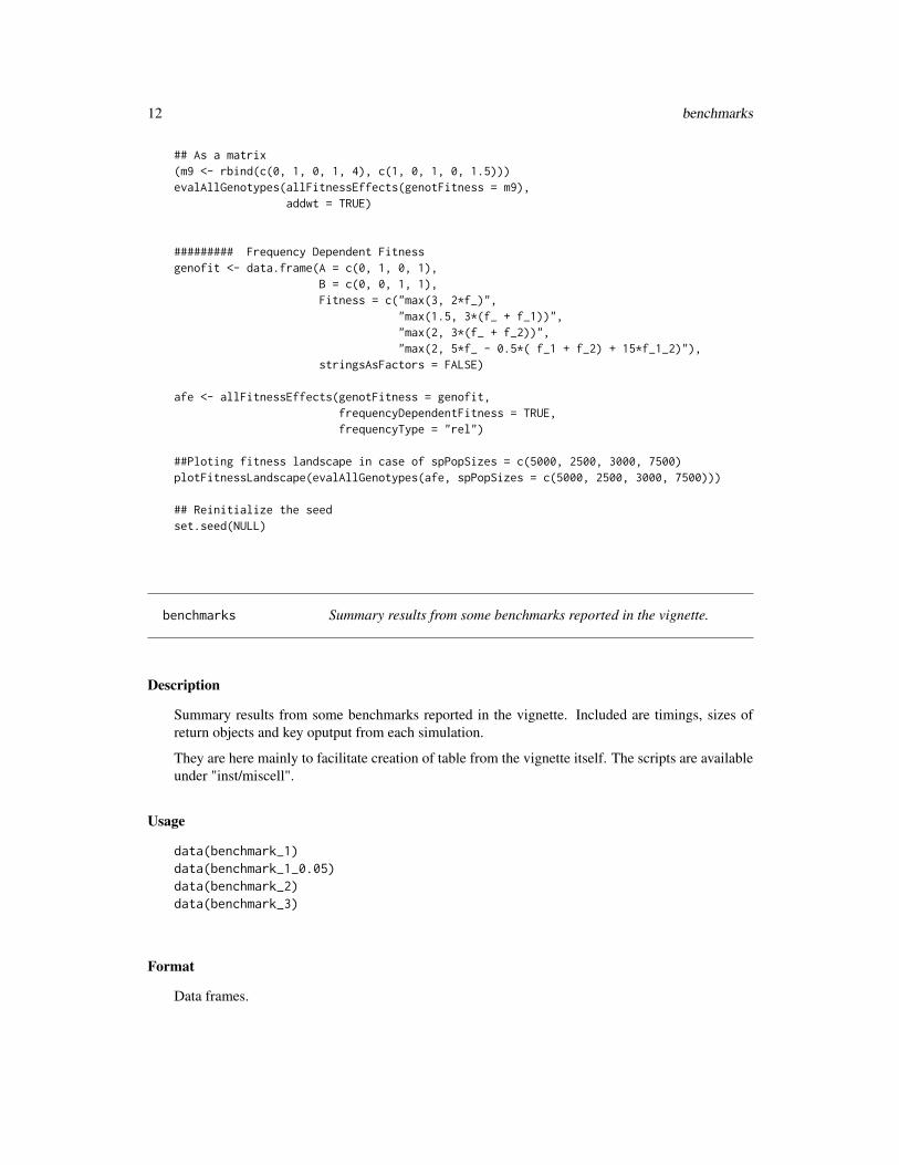
## As a matrix(m9 <- rbind(c(0, 1, 0, 1, 4), c(1, 0, 1, 0, 1.5)))evalAllGenotypes(allFitnessEffects(genotFitness = m9),
addwt = TRUE)
######### Frequency Dependent Fitnessgenofit <- data.frame(A = c(0, 1, 0, 1),
B = c(0, 0, 1, 1),Fitness = c("max(3, 2*f_)",
"max(1.5, 3*(f_ + f_1))","max(2, 3*(f_ + f_2))","max(2, 5*f_ - 0.5*( f_1 + f_2) + 15*f_1_2)"),
stringsAsFactors = FALSE)
afe <- allFitnessEffects(genotFitness = genofit,frequencyDependentFitness = TRUE,frequencyType = "rel")
##Ploting fitness landscape in case of spPopSizes = c(5000, 2500, 3000, 7500)plotFitnessLandscape(evalAllGenotypes(afe, spPopSizes = c(5000, 2500, 3000, 7500)))
## Reinitialize the seedset.seed(NULL)
benchmarks Summary results from some benchmarks reported in the vignette.
Description
Summary results from some benchmarks reported in the vignette. Included are timings, sizes ofreturn objects and key oputput from each simulation.
They are here mainly to facilitate creation of table from the vignette itself. The scripts are availableunder "inst/miscell".
Usage
data(benchmark_1)data(benchmark_1_0.05)data(benchmark_2)data(benchmark_3)
Format
Data frames.

evalAllGenotypes 13
Examples
data(benchmark_1)benchmark_1
evalAllGenotypes Evaluate fitness/mutator effects of one or all possible genotypes.
Description
Given a fitnessEffects/mutatorEffects description, obtain the fitness/mutator effects of a single orall genotypes.
Usage
evalGenotype(genotype, fitnessEffects, spPopSizes = NULL,verbose = FALSE, echo = FALSE, model = "",currentTime = 0)
evalGenotypeMut(genotype, mutatorEffects, spPopSizes = NULL,verbose = FALSE, echo = FALSE, currentTime = 0)
evalAllGenotypes(fitnessEffects, order = FALSE, max = 256, addwt = FALSE,model = "", spPopSizes = NULL, currentTime = 0)
evalAllGenotypesMut(mutatorEffects, max = 256, addwt = FALSE,spPopSizes = NULL, currentTime = 0)
evalGenotypeFitAndMut(genotype, fitnessEffects,mutatorEffects, spPopSizes = NULL,verbose = FALSE, echo = FALSE,model = "", currentTime = 0)
evalAllGenotypesFitAndMut(fitnessEffects, mutatorEffects,order = FALSE, max = 256, addwt = FALSE,model = "", spPopSizes = NULL, currentTime = 0)
Arguments
genotype (For evalGenotype). A genotype, as a character vector, with genes separatedby "," or ">", or as a numeric vector. Use the same integers or characters usedin the fitnessEffects object. This is a genotype in terms of genes, not modules.Using "," or ">" makes no difference: the sequence is always taken as the orderin which mutations occurred. Whether order matters or not is encoded in thefitnessEffects object.
fitnessEffects A fitnessEffects object, as produced by allFitnessEffects.

14 evalAllGenotypes
mutatorEffects A mutatorEffects object, as produced by allMutatorEffects.order (For evalAllGenotypes). If TRUE, then order matters. If order matters, then
generate not only all possible combinations of the genes, but all possible permu-tations for each combination.
max (For evalAllGenotypes). By default, no output is shown if the number ofpossible genotypes exceeds the max. Increase as needed.
addwt (For evalAllGenotypes). Add the wildtype (no mutations) explicitly? In caseof frequencyDependentFitness = TRUE the fitness of WT is always shown.
model Either nothing (the default) or "Bozic". If "Bozic" then the fitness effects con-tribute to decreasing the Death rate. Otherwise Birth rate is shown (and labeledas Fitness).
verbose (For evalGenotype). If set to TRUE, print out the individual terms that areadded to 1 (or subtracted from 1, if model is "Bozic").
echo (For evalGenotype). If set to TRUE, show the input genotype and print outa message with the death rate or fitness value. Useful for some examples, asshown in the vignette.
spPopSizes spPopSizes is only needed when frequencyDependentFitness = TRUE andyou want to evaluate fitness with evalGenotype or evalAllGenotypes (seethese functions for more info).spPopSizes is a numeric vector that contains the population sizes of the clones,in the same order of genotypes appear in the Genotype column of genotFitness.In your_object$full_FDF_spec you can see the genotypes (and the order) forwhich you need to pass the values (recall genotypes not specified explicitly aregiven a value of 0 and do not show up in this table).It is strongly recommended that spPopSizes be a named vector to allow forchecks and matches to the actual genotypes.
currentTime The time of the simulation. It is possible to access to the current time and run in-terventions for example using the frequency-dependent-fitness functionality ormodifying the mutation rate through oncoSimul functions such as oncoSimulIn-div. With evalAllGenotypes we can check if the fitness has changed before orafter a specific timepoint.
Value
For evalGenotype either the value of fitness or (if verbose = TRUE) the value of fitness and itsindividual components.
For evalAllGenotypes a data frame with two columns, the Genotype and the Fitness (or DeathRate, if Bozic). The notation for the Genotype colum is a follows: when order does not matter, acomma "," separates the identifiers of mutated genes. When order matters, a genotype shown as “x> y _ z” means that a mutation in “x” happened before a mutation in “y”; there is also a mutationin “z” (which could have happened before or after either of “x” or “y”), but “z” is a gene for whichorder does not matter. In all cases, a "WT" denotes the wild-type (or, actually, the genotype withoutany mutations).
If you use both fitnessEffects and mutatorEffects in a call, all the genes specified in mutatorEffectsMUST be included in the fitnessEffects object. If you want to have genes that have no direct ef-fect on fitness, but that affect mutation rate, you MUST specify them in the call to fitnessEffects,for instance as noIntGenes with an effect of 0.

evalAllGenotypes 15
When you are in a frequency dependent fitness situation you must set frequencydependentFitness= TRUE and spPopSizes must not be NULL and its length must be equal to the number of possiblegenotypes. Here only evalGenotype and evalAllGenotypes make sense.
Note
Fitness is used in a slight abuse of the language. Right now, mutations contribute to the birth ratefor all models except Bozic, where they modify the death rate. The general expression for fitnessis the usual multiplicative one of
∏(1 + si), where each si refers to the fitness effect of the given
gene. When dealing with death rates, we use∏(1− si).
Modules are, of course, taken into account if present (i.e., fitness is specified in terms of modules,but the genotype is specified in terms of genes).
About the naming. This is the convention used: "All" means we will go over all possible genotypes.A function that ends as "Genotypes" returns only fitness effects (for backwards compatibility andbecause mutator effects are not always used). A function that ends as "Genotype(s)Mut" returnsonly the mutator effects. A function that ends as "FitAndMut" will return both fitness and mutatoreffects.
Functions that return ONLY fitness or ONLY mutator effects are kept as separate functions becausethey free you from specifyin mutator/fitness effects if you only want to play with one of them.
Author(s)
Ramon Diaz-Uriarte, Sergio Sanchez Carrillo, Juan Antonio Miguel Gonzalez
See Also
allFitnessEffects.
Examples
# A three-gene epistasis examplesa <- 0.1sb <- 0.15sc <- 0.2sab <- 0.3sbc <- -0.25sabc <- 0.4
sac <- (1 + sa) * (1 + sc) - 1
E3A <- allFitnessEffects(epistasis =c("A:-B:-C" = sa,
"-A:B:-C" = sb,"-A:-B:C" = sc,"A:B:-C" = sab,"-A:B:C" = sbc,"A:-B:C" = sac,"A : B : C" = sabc)
)

16 evalAllGenotypes
evalAllGenotypes(E3A, order = FALSE, addwt = FALSE)evalAllGenotypes(E3A, order = FALSE, addwt = TRUE, model = "Bozic")
evalGenotype("B, C", E3A, verbose = TRUE)
## Order effects and modulesofe2 <- allFitnessEffects(orderEffects = c("F > D" = -0.3, "D > F" = 0.4),
geneToModule =c("Root" = "Root",
"F" = "f1, f2, f3","D" = "d1, d2") )
evalAllGenotypes(ofe2, order = TRUE, max = 325)[1:15, ]
## Next two are identicalevalGenotype("d1 > d2 > f3", ofe2, verbose = TRUE)evalGenotype("d1 , d2 , f3", ofe2, verbose = TRUE)
## This is differentevalGenotype("f3 , d1 , d2", ofe2, verbose = TRUE)## but identical to this oneevalGenotype("f3 > d1 > d2", ofe2, verbose = TRUE)
## Restrictions in mutations as a graph. Modules present.
p4 <- data.frame(parent = c(rep("Root", 4), "A", "B", "D", "E", "C", "F"),child = c("A", "B", "D", "E", "C", "C", "F", "F", "G", "G"),s = c(0.01, 0.02, 0.03, 0.04, 0.1, 0.1, 0.2, 0.2, 0.3, 0.3),sh = c(rep(0, 4), c(-.9, -.9), c(-.95, -.95), c(-.99, -.99)),typeDep = c(rep("--", 4),
"XMPN", "XMPN", "MN", "MN", "SM", "SM"))fp4m <- allFitnessEffects(p4,
geneToModule = c("Root" = "Root", "A" = "a1","B" = "b1, b2", "C" = "c1","D" = "d1, d2", "E" = "e1","F" = "f1, f2", "G" = "g1"))
evalAllGenotypes(fp4m, order = FALSE, max = 1024, addwt = TRUE)[1:15, ]
evalGenotype("b1, b2, e1, f2, a1", fp4m, verbose = TRUE)
## Of course, this is identical; b1 and b2 are same module## and order is not present here
evalGenotype("a1, b2, e1, f2", fp4m, verbose = TRUE)
evalGenotype("a1 > b2 > e1 > f2", fp4m, verbose = TRUE)
## We can use the exact same integer numeric id codes as in the## fitnessEffects geneModule component:
evalGenotype(c(1L, 3L, 7L, 9L), fp4m, verbose = TRUE)

evalAllGenotypes 17
## Epistasis for fitness and simple mutator effects
fe <- allFitnessEffects(epistasis = c("a : b" = 0.3,"b : c" = 0.5),
noIntGenes = c("e" = 0.1))
fm <- allMutatorEffects(noIntGenes = c("a" = 10,"c" = 5))
evalAllGenotypesFitAndMut(fe, fm, order = "FALSE")
## Simple fitness effects (noIntGenes) and modules## for mutators
fe2 <- allFitnessEffects(noIntGenes =c(a1 = 0.1, a2 = 0.2,
b1 = 0.01, b2 = 0.3, b3 = 0.2,c1 = 0.3, c2 = -0.2))
fm2 <- allMutatorEffects(epistasis = c("A" = 5,"B" = 10,"C" = 3),
geneToModule = c("A" = "a1, a2","B" = "b1, b2, b3","C" = "c1, c2"))
## Show only all the fitness effectsevalAllGenotypes(fe2, order = FALSE)
## Show only all mutator effectsevalAllGenotypesMut(fm2)
## Show all fitness and mutatorevalAllGenotypesFitAndMut(fe2, fm2, order = FALSE)
## This is probably not what you wanttry(evalAllGenotypesMut(fe2))## ... nor thistry(evalAllGenotypes(fm2))
## Show the fitness effect of a specific genotypeevalGenotype("a1, c2", fe2, verbose = TRUE)
## Show the mutator effect of a specific genotypeevalGenotypeMut("a1, c2", fm2, verbose = TRUE)
## Fitness and mutator of a specific genotypeevalGenotypeFitAndMut("a1, c2", fe2, fm2, verbose = TRUE)

18 example-missing-drivers
## This is probably not what you wanttry(evalGenotype("a1, c2", fm2, verbose = TRUE))
## Not what you want eithertry(evalGenotypeMut("a1, c2", fe2, verbose = TRUE))
## Frequency dependent fitness exampler <- data.frame(Genotype = c("WT", "A", "B", "A, B"),
Fitness = c("1 + 1.5*f_","5 + 3*(f_A + f_B + f_A_B)","5 + 3*(f_A + f_B + f_A_B)","7 + 5*(f_A + f_B + f_A_B)"),
stringsAsFactors = FALSE)
afe <- allFitnessEffects(genotFitness = r,frequencyDependentFitness = TRUE,frequencyType = "rel")
evalAllGenotypes(afe, spPopSizes = c(5000, 2500, 2500, 500))
example-missing-drivers
An example where there are intermediate missing drivers.
Description
An example where there are intermediate missing drivers. This is fictitious and I’ve never seen it.But it is here to check plots work even if there are no cases of some intermediate value of drivers (2in this case). b11 contains the full, original data, whereas b12 contains the same data where thereare no cases with exactly 2 drivers.
Usage
data("ex_missing_drivers_b11"); data("ex_missing_drivers_b12")
Format
Two objects of class "oncosimul".
See Also
plot.oncosimul

examplePosets 19
Examples
data(ex_missing_drivers_b11)plot(ex_missing_drivers_b11, type = "line")dev.new()data(ex_missing_drivers_b12)plot(ex_missing_drivers_b12, type = "line")
examplePosets Example posets
Description
Some example posets. For simplicity, all the posets are in a single list. You can access each posetby accessing each element of the list. The first digit or pair of digits denotes the number of nodes.
Poset 1101 is the same as the one in Gerstung et al., 2009 (figure 2A, poset 2). Poset 701 is thesame as the one in Gerstung et al., 2011 (figure 2B, left, the pancreatic cancer poset). Those posetswere entered manually at the command line: see poset.
Usage
data("examplePosets")
Format
The format is: List of 13 $ p1101: num [1:10, 1:2] 1 1 3 3 3 7 7 8 9 10 ... $ p1102: num [1:9, 1:2]1 1 3 3 3 7 7 9 10 2 ... $ p1103: num [1:9, 1:2] 1 1 3 3 3 7 7 8 10 2 ... $ p1104: num [1:9, 1:2] 1 1 33 7 7 9 2 10 2 ... $ p901 : num [1:8, 1:2] 1 2 4 5 7 8 5 1 2 3 ... $ p902 : num [1:6, 1:2] 1 2 4 5 7 5 23 5 6 ... $ p903 : num [1:6, 1:2] 1 2 5 7 8 1 2 3 6 8 ... $ p904 : num [1:6, 1:2] 1 4 5 5 1 7 2 5 8 6 ...$ p701 : num [1:9, 1:2] 1 1 1 1 2 3 4 4 5 2 ... $ p702 : num [1:6, 1:2] 1 1 1 1 2 4 2 3 4 5 ... $ p703: num [1:6, 1:2] 1 1 1 1 3 5 2 3 4 5 ... $ p704 : num [1:6, 1:2] 1 1 1 1 4 5 2 3 4 5 ... $ p705 : num[1:6, 1:2] 1 2 1 1 1 2 2 5 4 6 ...
Source
Gerstung et al., 2009. Quantifying cancer progression with conjunctive Bayesian networks. Bioin-formatics, 21: 2809–2815.
Gerstung et al., 2011. The Temporal Order of Genetic and Pathway Alterations in Tumorigenesis.PLoS ONE, 6.
See Also
poset

20 examplesFitnessEffects
Examples
data(examplePosets)
## Plot all of thempar(mfrow = c(3, 5))
invisible(sapply(names(examplePosets),function(x) {plotPoset(examplePosets[[x]],
main = x,box = TRUE)}))
examplesFitnessEffects
Examples of fitness effects
Description
Some examples of fitnessEffects objects. This is a collection, in a list, of most of the fitnessEf-fects created (using allFitnessEffects) for the vignette. See the vignette for descriptions andreferences.
Usage
data("examplesFitnessEffects")
Format
The format is a list of fitnessEffects objects.
See Also
allFitnessEffects
Examples
data(examplesFitnessEffects)
plot(examplesFitnessEffects[["fea"]])
evalAllGenotypes(examplesFitnessEffects[["cbn1"]], order = FALSE)

freq-dep-simul-examples 21
freq-dep-simul-examples
Runs from simulations of frequency-dependent examples shown in thevignette.
Description
Simulations shown in the vignette. Since running them can take a few seconds, we have pre-runthem, and stored the results.
Usage
data(woAntibS)
Format
For output from runs of oncoSimulIndiv a list of classes oncosimul and oncosimul2.
See Also
oncoSimulIndiv
Examples
data(woAntibS)plot(woAntibS, show = "genotypes", type = "line",
col = c("black", "green", "red"))
mcfLs mcfLs simulation from the vignette
Description
Trimmed output from the simulation mcfLs in the vignette. This is a somewhat long run, and wehave stored here the object (after trimming the Genotype matrix) to allow for plotting it.
Usage
data("mcfLs")
Format
An object of class "oncosimul2". A list.
See Also
plot.oncosimul

22 oncoSimulIndiv
Examples
## Not run:data(mcfLs)
plot(mcfLs, addtot = TRUE, lwdClone = 0.9, log = "")summary(mcfLs)
## End(Not run)
oncoSimulIndiv Simulate tumor progression for one or more individuals, optionallyreturning just a sample in time.
Description
Simulate tumor progression including possible restrictions in the order of driver mutations. Op-tionally add passenger mutations. When used in frequency dependent fitness situation, only fitnesseffects are allowed. Simulation is done using the BNB algorithm of Mather et al., 2012.
Usage
oncoSimulIndiv(fp, model = "Exp",numPassengers = 0, mu = 1e-6, muEF = NULL,detectionSize = 1e8, detectionDrivers = 4,detectionProb = NA,sampleEvery = ifelse(model %in% c("Bozic", "Exp"), 1,
0.025),initSize = 500, s = 0.1, sh = -1,K = sum(initSize)/(exp(1) - 1), keepEvery = sampleEvery,minDetectDrvCloneSz = "auto",extraTime = 0,finalTime = 0.25 * 25 * 365, onlyCancer = TRUE,keepPhylog = FALSE,mutationPropGrowth = ifelse(model == "Bozic",
FALSE, TRUE),max.memory = 2000, max.wall.time = 200,max.num.tries = 500,errorHitWallTime = TRUE,errorHitMaxTries = TRUE,verbosity = 0,initMutant = NULL,AND_DrvProbExit = FALSE,fixation = NULL,seed = NULL)
oncoSimulPop(Nindiv, fp, model = "Exp", numPassengers = 0, mu = 1e-6,muEF = NULL,

oncoSimulIndiv 23
detectionSize = 1e8, detectionDrivers = 4,detectionProb = NA,sampleEvery = ifelse(model %in% c("Bozic", "Exp"), 1,
0.025),initSize = 500, s = 0.1, sh = -1,K = sum(initSize)/(exp(1) - 1), keepEvery = sampleEvery,minDetectDrvCloneSz = "auto",extraTime = 0,finalTime = 0.25 * 25 * 365, onlyCancer = TRUE,keepPhylog = FALSE,mutationPropGrowth = ifelse(model == "Bozic",
FALSE, TRUE),max.memory = 2000, max.wall.time = 200,max.num.tries = 500,errorHitWallTime = TRUE,errorHitMaxTries = TRUE,initMutant = NULL,AND_DrvProbExit = FALSE,fixation = NULL,verbosity = 0,mc.cores = detectCores(),seed = "auto")
oncoSimulSample(Nindiv,fp,model = "Exp",numPassengers = 0,mu = 1e-6,muEF = NULL,detectionSize = round(runif(Nindiv, 1e5, 1e8)),
detectionDrivers = {if(inherits(fp, "fitnessEffects")) {
if(length(fp$drv)) {nd <- (2: round(0.75 * length(fp$drv)))
} else {nd <- 9e6
}} else {
nd <- (2 : round(0.75 * max(fp)))}if (length(nd) == 1)
nd <- c(nd, nd)sample(nd, Nindiv,
replace = TRUE)},
detectionProb = NA,

24 oncoSimulIndiv
sampleEvery = ifelse(model %in% c("Bozic", "Exp"), 1,0.025),
initSize = 500,s = 0.1,sh = -1,K = sum(initSize)/(exp(1) - 1),minDetectDrvCloneSz = "auto",extraTime = 0,finalTime = 0.25 * 25 * 365,onlyCancer = TRUE, keepPhylog = FALSE,mutationPropGrowth = ifelse(model == "Bozic",
FALSE, TRUE),max.memory = 2000,max.wall.time.total = 600,max.num.tries.total = 500 * Nindiv,typeSample = "whole",thresholdWhole = 0.5,initMutant = NULL,AND_DrvProbExit = FALSE,fixation = NULL,verbosity = 1,showProgress = FALSE,seed = "auto")
Arguments
Nindiv Number of individuals or number of different trajectories to simulate.
fp Either a poset that specifies the order restrictions (see poset if you want to usethe specification as in v.1. Otherwise, a fitnessEffects object (see allFitnessEffects).You must always use a fitnessEffects object when you are in a frequency depen-dent fitness simulation; of course in this case fp$frequencyDependentFitnessmust be TRUE.Other arguments below (s, sh, numPassengers) make sense only if you use aposet, as they are included in the fitnessEffects object.
model One of "Bozic", "Exp", "McFarlandLog", "McFarlandLogD" (the last two canbe abbreviated to "McFL" and "McFLD", respectively). The default is "Exp".(See vignette for the difference between "McFL" and "McFLD": in the former,death rate = log(1 + N/K) where K is the initial equilibrium population size;when using "McFLD", death rate = max(1, log(1 + N/K)), so that death ratenever goes below 1.)
numPassengers This has no effect if you use the allFitnessEffects specification. This hap-pens always when you are in a simulation that use frequency dependent fitness.If you use the specification of v.1., the number of passenger genes. Note thatusing v.1 the total number of genes (drivers plus passengers) must be smallerthan 64.

oncoSimulIndiv 25
All driver genes should be included in the poset (even if they depend on no oneand no one depends on them), and will be numbered from 1 to the total numberof driver genes. Thus, passenger genes will be numbered from (number of drivergenes + 1):(number of drivers + number of passengers).
mu Mutation rate. Can be a single value or a named vector. If a single value,all genes will have the same mutation rate. If a named vector, the entriesin the vector specify the gene-specific mutation rate. If you pass a vector, itmust be named, and it must have entries for all the genes in the fitness spec-ification. Passing a vector is only available when using fitnessEffects objectsfor fitness specification. Mutation rates <10^-20 are not accepted. See alsomutationPropGrowth.
muEF Mutator effects. A mutatorEffects object as obtained from allMutatorEffects.This specifies how mutations in certain genes change the mutation rate over allthe genome. Therefore, this allows you to specify mutator phenotypes: modelswhere mutation of one (or more) gene(s) leads to an increase in the mutationrate. This is only available for version 2 (and above) specifications.All the genes specified in muEF MUST be included in fp. If you want to havegenes that have no direct effect on fitness, but that affect mutation rate, youMUST specify them in fp, for instance as noIntGenes with an effect of 0.If you use mutator effects you must also use fitnessEffects in fp.
detectionSize What is the minimal number of cells for cancer to be detected. For oncoSimulSamplethis can be a vector.If set to NA, detectionSize plays no role in stopping the simulations.
detectionDrivers
The minimal number of drivers (not modules, drivers, whether or not they arefrom the same module) present in any clone for cancer to be detected. ForoncoSimulSample this can be a vector.For oncoSimulSample, if there are drivers (either because you are using a v.1object or because you are using a fitnessEffects object with a drvNames com-ponent —see allFitnessEffects—) the default is a vector of drivers from auniform between 2 and 0.75 the total number of drivers. If there are no drivers(because you are using a fitnessEffects object without a drvNames, either be-cause you specified it explicitly or because all of the genes are in the noIntGenescomponent) the simulations should not stop based on the number of drivers (and,thus, the default is set to 9e6). This is the case when you run the simulation withfrequency dependent fitness.If set to NA, detectionDrivers plays no role in stopping the simulations.
detectionProb Vector of arguments for the mechanism where probability of detection dependson size. If NA, this mechanism is not used. If ‘default’, the vector will be popu-lated with default values. Otherwise, a named vector with some of the followingnamed elements (see ‘Details’):
• PDBaseline: Baseline size subtracted to total population size to computethe probability of detection. If not given explicitly, the default is 1.2 *initSize (or 1.2 * sum(initSize) when multiple initMutants).
• p2: The probability of detection at population size n2. If you specificy p2you must also specify n2 and you must not specify cPDetect. The fault is0.1.

26 oncoSimulIndiv
• n2: The population size at which probability of detection is p2. The defaultis 2 * initSize.
• cPDetect: The change in probability of detection with size. If you specifyit, you should not specify either of p2 or n2. See ‘Details’.
• checkSizePEvery: Time between successive checks for the probability ofexiting as a function of population size. If not given explicitly, the defaultis 20. See ‘Details’.
If you only provide some of the elements (except for the pair p2, n2, where youmust provide both if you provide any), the rest will be filled with default values.This option can not be used with v.1 objects.
sampleEvery How often the whole population is sampled. This is not the same as the intervalbetween successive samples that are kept or stored (for that, see keepEvery).For very fast growing clones, you might need to have a small value here to min-imize possible numerical problems (such as huge increase in population size be-tween two successive samples that can then lead to problems for random numbergenerators). Likewise, for models with density dependence (such as McF) thisvalue should be very small.
initSize Initial population size. If you are passing more than one initMutant, the initialpopulation sizes of each clone/species/genotype, given in the same order as inthe initMutant vector. initMutant thus allows to start the simulation fromarbitrary population compositions. Combined with mu it allows for multispeciessimulations (see the vignette for examples).
K Initial population equilibrium size in the McFarland models.
keepEvery Time interval between successive whole population samples that are actuallystored. This must be larger or equal to sampleEvery. If keepEvery is not amultiple integer of sampleEvery, the interval between successive samples thatare stored will be the smallest multiple integer of sampleEvery that is largerthan or equal to keepEvery.If you want nice plots, set sampleEvery and keepEvery to small values (say, 5or 2). Otherwise, you can use a sampleEvery of 1 but a keepEvery of 15, sothat the return objects are not huge and the code runs a lot faster.Setting keepEvery = NA means we only keep the very last sample. This is usefulif you only care about the final state of the simulation, not its complete history.
minDetectDrvCloneSz
A value of 0 or larger than 0 (by default equal to initSize in the McFarlandmodel). If larger than 0, when checking if we are done with a simulation, weverify that the sum of the population sizes of all clones that have a number ofmutated drivers larger or equal to detectionDrivers is larger or equal to thisminDetectDrvCloneSz.The reason for this parameter is to ensure that, say, a clone with a certain numberof drivers that would cause the simulation to end has not just appeared and ispresent in only one individual that might then immediately go extinct. This canbe relevant in secenarios such as the McFarland model.If initSize is larger than 1 (you are passing multiple initMutants), the sum isused.See also extraTime.

oncoSimulIndiv 27
extraTime A value larger than zero waits those many additional time periods before exitingafter having reached the exit condition (population size, number of drivers).The reason for this setting is to prevent the McFL models from always exiting ata time when one clone is increasing its size quickly (see minDetectDrvCloneSz).By setting an extraTime larger than 0, we can sample at points when we are atthe plateau.
finalTime What is the maximum number of time units that the simulation can run. Set toNA to disable this limit.
onlyCancer Return only simulations that reach cancer?If set to TRUE, only simulations that satisfy the detectionDrivers or thedetectionSize requirements or that are "detected" because of the detectionProbmechanism will be returned: the simulation will be repeated, within the limitsset by max.num.tries and max.wall.time (and, for oncoSimulSample alsomax.num.tries.total and max.wall.time.total), until one which meets thedetectionDrivers or detectionSize or one which is detected stochasticallyunder detectionProb is obtained.If onlyCancer = FALSE the simulation is returned regardless of final populationsize or number of drivers in any clone and this includes simulations where thepopulation goes extinct.
keepPhylog If TRUE, keep track of when and from which clone each clone is created. Seealso plotClonePhylog.
mutationPropGrowth
If TRUE, make mutation rate proportional to growth rate, so clones that growfaster also mutate faster (laso have a larger mutation rate): $mutation_rate =mu * birth_rate$. With BNB mutation is actually "mutate after division": p.\1232 of Mather et al., 2012 explains: "(...) mutation is simply defined as thecreation and subsequent departure of a single individual from the class". Thus,if we want to have individuals of clones/genotypes/populations that divide fasterto also produce more mutants per unit time (per individual) we have to setmutationPropGrowth = TRUE.Of course, this only makes sense in models where birth rate changes.
initMutant For v.2: a string with the mutations of the initial mutant, if any. This is the sameformat as for evalGenotype. The default (if you pass nothing) is to start thesimulation from the wildtype genotype with nothing mutated. For v.1 we nolonger accept initMutant: it will be ignored.(evalGenotype also accepts the genotype as a numeric vector; initMutantmust be a character string.)
max.num.tries Only applies when onlyCancer = TRUE. What is the maximum number of times,for an individual simulation, we can repeat the simulation for it to reach cancer?There are certain parameter settings where reaching cancer is extremely unlikelyand you might not want to run forever in those cases.
max.num.tries.total
Only applies when onlyCancer = TRUE and for oncoSimulSample. What is themaximum number of times, over all simulations for all individuals in a popu-lation sample, that we can repeat the simulations so that cancer is reached forall individuals? The idea is to set a limit on the average minimal probability ofreaching cancer for a set of simulations to be accepted.

28 oncoSimulIndiv
max.wall.time Maximum wall time for the simulation of one individual (over all max.num.tries).If the simulation is not done in this time, it is aborted.
max.wall.time.total
Maximum wall time for all the simulations (when using oncoSimulSample),in seconds. If the simulation is not completed in this time, it is aborted. Toprevent problems from a single individual simulation going wild, this limit isalso enforced per simulation (so the run can be aborted directly from C++).
errorHitMaxTries
If TRUE (the default) a simulation that reaches the maximum number of repeti-tions allowed is considered not to have succesfully finished and, thus, an error,and no output from it will be reported. This is often what you want.See Details.
errorHitWallTime
If TRUE (the default) a simulation that reaches the maximum wall time is con-sidered not to have succesfully finished and, thus, an error, and no output fromit will be reported. This is often what you want.See Details.
max.memory The largest size (in MB) of the matrix of Populations by Time. If it creating itwould use more than this amount of memory, it is not created. This prevents youfrom accidentally passing parameters that will return an enormous object.
verbosity If 0, run silently. Iincreasing values of verbosity provide progressively moreinformation about intermediate steps, possible numerical notes/warnings fromthe C++ code, etc. Values less than 0 supress some default notes: use with care.
typeSample "singleCell" (or "single") for single cell sampling, where the probability of sam-pling a cell (a clone) is directly proportional to its population size. "wholeTu-mor" (or "whole") for whole tumor sampling (i.e., this is similar to a biopsybeing the entire tumor). See samplePop.
thresholdWhole In whole tumor sampling, whether a gene is detected as mutated depends onthresholdWhole: a gene is considered mutated if it is altered in at least thresh-oldWhole proportion of the cells in that individual. See samplePop.
mc.cores Number of cores to use when simulating more than one individual (i.e., whencalling oncoSimulPop).
showProgress If TRUE, provide information, during exection, of the individual done, and thenumber of attempts and time used.
AND_DrvProbExit
If TRUE, cancer will be considered to be reached if both the detectionProbmechanism and detectionDrivers are satisfied. This is and AND, not an ORcondition. Using this option with fixation is not allowed (as it does not makemuch sense).
fixation If non-NULL, a list or a vector, where each element of is a string with a geneor a gene combination or a genotype (see below). Simulations will stop as soonas any of the genes or gene combinations or genotypes are fixed (i.e., reach aminimal frequency). If you pass gene combinations or genotypes, separate geneswith commas (not ’>’); this means order is not (yet?) supported. This way ofspecifying gene combinations is the same as the one used for initMutant andevalGenotype.

oncoSimulIndiv 29
To differentiate between gene combinations and specific genotypes, genotypesare specified by prepending them with a "_,". For instance, fixation = c("A","B,C")specifies stopping on any genotypes with those gene combinations. In contrast,fixation = c("_,A","_,B,C" ) specifies stopping only on gentoypes "A" or"B, C". See the vignette for further examples.
In addition to the gene combinations or genotypes themeselves, you can add tothe list or vector the named elements fixation_tolerance, min_successive_fixationand fixation_min_size. fixation_tolerance: fixation is considered to havehappened if the genotype/gene combinations specified as genotypes/gene com-binations for fixation have reached a frequency > 1 -fixation_tolerance. (Thedefault is 0, so we ask for genotypes/gene combinations with a frequency of 1,which might not be what you want with large mutation rates and complex fitnesslandscape with genotypes of similar fitness.). min_successive_fixation: dur-ing how many successive sampling periods the conditions of fixation need to befulfilled before declaring fixation. These must be successive sampling periodswithout interruptions (i.e., a single period when the condition is not fulfilled willset the counter to 0). This can help to exclude short, transitional, local maximathat are quickly replaced by other genotypes. (The default is 50, but this is prob-ably too small for “real life” usage). fixation_min_size: you might only wantto consider fixation to have happened if a minimal size has been reached (thiscan help weed out local maxima that have fitness that is barely above that of thewild-type genotype). (The default is 0).
Using this option with AND_DrvProbExit is not allowed (as it does not makemuch sense). This option is not allowed either with the old v.1 specification.
s Selection coefficient for drivers. Only relevant if using a poset as this is includedin the fitnessEffects object. This will eventually be deprecated.
sh Selection coefficient for drivers with restrictions not satisfied. A value of 0means there are no penalties for a driver appearing in a clone when its restric-tions are not satisfied.
To specify "sh=Inf" (in Diaz-Uriarte, 2015) use sh = -1.
Only relevant if using a poset as this is included in the fitnessEffects object. Thiswill eventually be deprecated.
seed The seed for the C++ PRNG. You can pass a value. If you set it to NULL, thena seed will be generated in R and passed to C++. If you set it to "auto", thenif you are using v.1, the behavior is the same as if you set it to NULL (a seedwill be generated in R and passed to C++) but if you are using v.2, a randomseed will be produced in C++. If you need reproducibility, either pass a value orset it to NULL (setting it to NULL will make the C++ seed reproducible if youuse the same seed in R via set.seed). However, even using the same value ofseed is unlikely to give the exact same results between platforms and compilers.Moreover, note that the defaults for seed are not the same in oncoSimulIndiv,oncoSimulPop and oncoSimulSample.
When using oncoSimulPop, if you want reproducibility, you might want to, inaddition to setting seed = NULL, also do RNGkind("L'Ecuyer-CMRG") as we usemclapply; look at the vignette of parallel.

30 oncoSimulIndiv
Details
The basic simulation algorithm implemented is the BNB one of Mather et al., 2012, where I haveadded modifications to fitness based on the restrictions in the order of mutations.
Full details about the algorithm are provided in Mather et al., 2012. The evolutionary models,including references, and the rest of the parameters are explained in Diaz-Uriarte, 2014, especiallyin the Supplementary Material. The model called "Bozic" is based on Bozic et al., 2010, and themodel called "McFarland" in McFarland et al., 2013.
oncoSimulPop simply calls oncoSimulIndiv multiple times. When run on POSIX systems, it canuse multiple cores (via mclapply).
The summary methods for these classes return some of the return values (see next) as a one-row(for class oncosimul) or multiple row (for class oncosimulpop) data frame. The print methods forthese classes simply print the summary.
Changing options errorHitMaxTries and errorHitWallTime can be useful when conductingmany simulations, as in the call to oncoSimulPop: setting them to TRUE means nothing is recordedfor those simulations where ending conditions are not reached but setting them to FALSE wouldallow you to record the output; this would potentially result in a mixture where some simulationswould not have reached the ending condition, but this might sometimes be what you want. Note,however, that oncoSimulSample always has both them to TRUE, as it could not be otherwise.
GenotypesWDistinctOrderEff provides the information about order effects that is missing fromGenotypes. When there are order effects, the Genotypes matrix can contain genotypes that arenot distinguishable. Suppose there are two genes, the first and the second. In the Genotypeoutput you can get two columns where there is a 1 in both genes: those two columns corre-spond to the two possible orders (first gene mutated first, or first gene mutated after the second).GenotypesWDistinctOrderEff disambiguates this. The same is done by GenotypesLabels; thisis easier to decode for a human (a string of gene labels) but a little bit harder to parse automatically.Note that when you use the default print method for this object, you get, among others, a two-column display with the GenotypeLabels information. When order matters, a genotype shown as“x > y _ z” means that a mutation in “x” happened before a mutation in “y”; there is also a mutationin “z” (which could have happened before or after either of “x” or “y”), but “z” is a gene for whichorder does not matter. When order does not matter, a comma "," separates the identifiers of mutatedgenes.
Detection of cancer can be a deterministic process, where cancer is always detected (and, thus, sim-ulation ended) when certain conditions are met (detectionSize, detectionDrivers, fixation).Alternatively, it can be stochastic process where probability of detection depends on size. Every sooften (see below) we assess population size, and detect cancer or not probabilistically (comparingthe probability of detection for that size with a random uniform number). Probability of detectionchanges with population size according to the function
1− e−cPDetect((populationsize−PDBaseline)/PDBaseline)
.
You can pass cPDetect manually (you will need to set n2 and p2 to NA). However, it might be moreintuitive to specify the pair n2, p2, such that the probability of detection is p2 for population size n2(and from that pair we solve for the value of cPDetect). How often do we check? That is controlledby checkSizePEvery, the (minimal) time between successive checks (from among the samplingtimes given by sampleEvery: the interval between successive assessments will be the smallest

oncoSimulIndiv 31
multiple integer of sampleEvery that is larger than checkSizePEvery —see vignette for details).checkSizePEvery has, by default, a different (and much larger) value than sampleEvery both toallow to examine the effects of sampling, and to avoid many costly random number generations.
Please note that detectionProb is NOT available with version 1 objects.
Value
For oncoSimulIndiv a list, of class "oncosimul", with the following components:
pops.by.time A matrix of the population sizes of the clones, with clones in columns and timein row. Not all clones are shown here, only those that were present in at least onof the keepEvery samples.
NumClones Total number of clones in the above matrix. This is not the total number ofdistinct clones that have appeared over all simulations (which is likely to belarger or much larger).
TotalPopSize Total population size at the end.
Genotypes A matrix of genotypes. For each of the clones in the pops.by.time matrix, itsgenotype, with a 0 if the gene is not mutated and a 1 if it is mutated.
MaxNumDrivers The largest number of mutated driver genes ever seen in the simulation in anyclone.
MaxDriversLast The largest number of mutated drivers in any clone at the end of the simulation.NumDriversLargestPop
The number of mutated driver genes in the clone with largest population size.
LargestClone Population size of the clone with largest number of population size.PropLargestPopLast
Ratio of LargestClone/TotalPopSize
FinalTime The time (in time units) at the end of the simulation.
NumIter The number of iterations of the BNB algorithm.
HittedWallTime TRUE if we reached the limit of max.wall.time. FALSE otherwise.TotalPresentDrivers
The total number of mutated driver genes, whether or not in the same clone. Thenumber of elements in OccurringDrivers, below.
CountByDriver A vector of length number of drivers, with the count of the number of clonesthat have that driver mutated.
OccurringDrivers
The actual number of drivers mutated.
PerSampleStats A 5 column matrix with a row for each sampling period. The columns are: totalpopulation size, population size of the largest clone, the ratio of the two, thelargest number of drivers in any clone, and the number of drivers in the clonewith the largest population size.
other A list that contains statistics for an estimate of the simulation error when us-ing the McFarland model as well as other statistics. For the McFarland model,the relevant value is errorMF, which is -99 unless in the McFarland model. Forthe McFarland model it is the largest difference of successive death rates. The

32 oncoSimulIndiv
entries named minDMratio and minBMratio are the smallest ratio, over all simu-lations, of death rate to mutation rate and birth rate to mutation rate, respectively.The BNB algorithm thrives when those are large.
For oncoSimulPop a list of length Nindiv, and of class "oncosimulpop", where each element ofthe list is itself a list, of class oncosimul, with components as described above.
In v.2, the output is of both class "oncosimul" and "oncosimul2". The oncoSimulIndiv return objectdiffers in
GenotypesWDistinctOrderEff
A list of vectors, where each vector corresponds to a genotype in the Genotypes,showing (where it matters) the order of mutations. Each vector shows the geno-types, with the numeric codes, showing explicitly the order when it matters. Soif you have genes 1, 2, 7 for which order relationships are given, and genes 3, 4,5, 6 for which other interactions exist, any mutations in 1, 2, 7 are shown first,and in the order they occurred, before showing the rest of the mutations. Seedetails.
GenotypesLabels
The genotypes, as character vectors with the original labels provided (i.e., notthe integer codes). As before, mutated genes, for those where order matters,come first, and are separated by the rest by a "_". See details.
OccurringDrivers
This is the same as in v.1, but we use the labels, not the numeric id codes. Ofcourse, if you entered integers as labels for the genes, you will see numbers(however, as a character string).
Note
Please, note that the meaning of the fitness effects in the McFarland model is not the same as in theoriginal paper; the fitness coefficients are transformed to allow for a simpler fitness function as aproduct of terms. This differs with respect to v.1. See the vignette for details.
Author(s)
Ramon Diaz-Uriarte
References
Bozic, I., et al., (2010). Accumulation of driver and passenger mutations during tumor progression.Proceedings of the National Academy of Sciences of the United States of America\/, 107, 18545–18550.
Diaz-Uriarte, R. (2015). Identifying restrictions in the order of accumulation of mutations dur-ing tumor progression: effects of passengers, evolutionary models, and sampling http://www.biomedcentral.com/1471-2105/16/41/abstract
Gerstung et al., 2011. The Temporal Order of Genetic and Pathway Alterations in Tumorigenesis.PLoS ONE, 6.
McFarland, C.~D. et al. (2013). Impact of deleterious passenger mutations on cancer progression.Proceedings of the National Academy of Sciences of the United States of America\/, 110(8), 2910–5.

oncoSimulIndiv 33
Mather, W.~H., Hasty, J., and Tsimring, L.~S. (2012). Fast stochastic algorithm for simulatingevolutionary population dynamics. Bioinformatics (Oxford, England)\/, 28(9), 1230–1238.
See Also
plot.oncosimul, samplePop, allFitnessEffects
Examples
#### A model similar to the one in McFarland. We use 270 genes.
set.seed(456)nd <- 70np <- 200s <- 0.1sp <- 1e-3spp <- -sp/(1 + sp)mcf1 <- allFitnessEffects(noIntGenes = c(rep(s, nd), rep(spp, np)),
drv = seq.int(nd))mcf1s <- oncoSimulIndiv(mcf1,
model = "McFL",mu = 1e-7,detectionSize = 1e8,detectionDrivers = 100,sampleEvery = 0.02,keepEvery = 2,initSize = 2000,finalTime = 1000,onlyCancer = FALSE)
plot(mcf1s, addtot = TRUE, lwdClone = 0.6, log = "")summary(mcf1s)plot(mcf1s)
#### Order effects with modules, and 5 genes without interactions#### with fitness effects from an exponential distribution
oi <- allFitnessEffects(orderEffects =c("F > D" = -0.3, "D > F" = 0.4),noIntGenes = rexp(5, 10),
geneToModule =c("Root" = "Root",
"F" = "f1, f2, f3","D" = "d1, d2") )
oiI1 <- oncoSimulIndiv(oi, model = "Exp")oiI1$GenotypesLabelsoiI1 ## note the order and separation by "_"
oiP1 <- oncoSimulPop(2, oi,keepEvery = 10,

34 oncoSimulIndiv
mc.cores = 2)summary(oiP1)
## Even if order exists, this cannot reflect it;## G1 to G10 are d1, d2, f1..,f3, and the 5 genes without## interactionsamplePop(oiP1)
oiS1 <- oncoSimulSample(2, oi)
## The output contains only the summary of the runs AND## the sample:oiS1
## And their sizes do differobject.size(oiS1)object.size(oiP1)
######## Using an extended poset for pancreatic cancer from Gerstung et al.### (s and sh are made up for the example; only the structure### and names come from Gerstung et al.)
pancr <- allFitnessEffects(data.frame(parent = c("Root", rep("KRAS", 4), "SMAD4", "CDNK2A","TP53", "TP53", "MLL3"),
child = c("KRAS","SMAD4", "CDNK2A","TP53", "MLL3",rep("PXDN", 3), rep("TGFBR2", 2)),
s = 0.05,sh = -0.3,typeDep = "MN"))
plot(pancr)
### Use an exponential growth model(pancr1 <- oncoSimulIndiv(pancr, model = "Exp"))
summary(pancr1)plot(pancr1)
## Pop and SamplepancrPop <- oncoSimulPop(2,
pancr,keepEvery = 10,mc.cores = 2)
summary(pancrPop)(pancrSPop <- samplePop(pancrPop))
(pancrSamp <- oncoSimulSample(2, pancr))

oncoSimulIndiv 35
## Not run:## Using gene-specific mutation ratesmuv <- c("U" = 1e-3, "z" = 1e-7, "e" = 1e-6, "m" = 1e-5, "D" = 1e-4)ni <- rep(0.01, 5)names(ni) <- names(muv)femuv <- allFitnessEffects(noIntGenes = ni)oncoSimulIndiv(femuv, mu = muv)
## End(Not run)
######### Frequency dependent fitness examples
## An example with cooperation. Presence of WT favours all clones## and all clones have a positive effect on themselvesgenofit <- data.frame(A = c(0, 1, 0, 1),
B = c(0, 0, 1, 1),Fitness = c("3 + 5*f_",
"3 + 5*(f_ + f_A)","3 + 5*(f_ + f_B)","5 + 6*(f_ + f_A_B)"))
afe <- allFitnessEffects(genotFitness = genofit,frequencyDependentFitness = TRUE)
## Use gene-specific mutation rates and start the simulation from## 5000 WT and 1000 A mutants.osi <- oncoSimulIndiv(afe,
model = "McFL",onlyCancer = FALSE,finalTime = 50,mu = c("A" = 1e-6, B = 1e-8),initMutant = c("WT", "A"),initSize = c(5000, 1000),keepPhylog = FALSE,seed = NULL,errorHitMaxTries = FALSE,errorHitWallTime = FALSE)
osi
plot(osi, show = "genotypes", type = "line")
## Not run:## This can be slowosp <- oncoSimulPop(5,
afe,model = "McFL",initSize = 5000,mu = 1e-6,keepEvery = 5,

36 oncoSimulIndiv
mc.cores = 2,finalTime = 5000)
sp <- samplePop(osp)
sp
## End(Not run)
## A little bit more complex example situation. WT favours clones A and B. A and## B compete with each other. Presence of A and B favours clone A, B.## Not run:## This can be slow
genofit <- data.frame(A = c(0, 1, 0, 1),B = c(0, 0, 1, 1),Fitness = c("3 + 5*f_",
"3 + 5*(f_ + f_1 - f_2)","3 + 5*(f_ + f_2 - f_1)","5 + 6*(f_1 + f_2 + f_1_2)"))
afe <- allFitnessEffects(genotFitness = genofit,frequencyDependentFitness = TRUE,frequencyType = "rel")
osi <- oncoSimulIndiv(afe,model = "McFL",onlyCancer = FALSE,finalTime = 200,mu = 1e-6,initSize = 5000,keepPhylog = FALSE,seed = NULL,errorHitMaxTries = FALSE,errorHitWallTime = FALSE)
osi
plot(osi, show = "genotypes", type = "line")
## End(Not run)## Not run:## This can be slowosp <- oncoSimulPop(5,
afe,model = "McFL",initSize = 5000,onlyCancer = FALSE,mu = 1e-6,keepEvery = 5,mc.cores = 2)
summary(osp)

OncoSimulWide2Long 37
sp <- samplePop(osp)
sp
oss <- oncoSimulSample(5,afe,model = "McFL",initSize = 5000,mu = 1e-6,finalTime = 5000,verbosity = 0)
oss
## End(Not run)
## Reinitialize the RNGset.seed(NULL)
OncoSimulWide2Long Convert the pops.by.time component of an oncosimul object into"long" format.
Description
Convert the pops.by.time component from its "wide" format (with one column for time, and asmany columns as clones/genotypes) into "long" format, so that it can be used with other functions,for instance for plots.
Usage
OncoSimulWide2Long(x)
Arguments
x An object of class oncosimul or oncosimul2.
Value
A data frame with four columns: Time; Y, the number of cells (the population size); Drivers, afactor with the number of drivers of the given genotype; Genotype, the genotyp.
Author(s)
Ramon Diaz-Uriarte
38 plot.fitnessEffects
See Also
oncoSimulIndiv
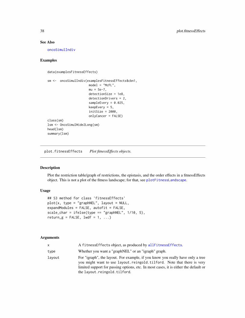
Examples
data(examplesFitnessEffects)
sm <- oncoSimulIndiv(examplesFitnessEffects$cbn1,model = "McFL",mu = 5e-7,detectionSize = 1e8,detectionDrivers = 2,sampleEvery = 0.025,keepEvery = 5,initSize = 2000,onlyCancer = FALSE)
class(sm)lsm <- OncoSimulWide2Long(sm)head(lsm)summary(lsm)
plot.fitnessEffects Plot fitnessEffects objects.
Description
Plot the restriction table/graph of restrictions, the epistasis, and the order effects in a fitnessEffectsobject. This is not a plot of the fitness landscape; for that, see plotFitnessLandscape.
Usage
## S3 method for class 'fitnessEffects'plot(x, type = "graphNEL", layout = NULL,expandModules = FALSE, autofit = FALSE,scale_char = ifelse(type == "graphNEL", 1/10, 5),return_g = FALSE, lwdf = 1, ...)
Arguments
x A fitnessEffects object, as produced by allFitnessEffects.
type Whether you want a "graphNEL" or an "igraph" graph.
layout For "igraph", the layout. For example, if you know you really have only a treeyou might want to use layout.reingold.tilford. Note that there is verylimited support for passing options, etc. In most cases, it is either the default orthe layout.reingold.tilford.
plot.fitnessEffects 39
expandModules If there are modules with multiple genes, if you set this to TRUE modules willbe replaced by their genes.
autofit If TRUE, we try to fit the edges to the labels. This is a very experimental feature,likely to be not very robust.
scale_char If using autofit = TRUE, the scaling factor for the size of the rectangles as afunction of the number of characters. You have to play with this because thebest value can depend on a number of things.
return_g It TRUE, the graph object (graphNEL or igrap) is returned.
lwdf The multiplier factor for lwd when using "graphNEL".
... Other arguments passed to plot. Not used for now.
Value
A plot.
Order and epistatic relationships have orange edges. OR (semimonotone) relationships blue, andXOR red. All others have black edges (so AND and unique edges from root). Epistatic rela-tionships, being symmetrical, have no arrows between nodes and have a dotted line type. Orderrelationships have an arrow from the earlier to the later event and have a different dotted line (lty 3).
If return_g is TRUE, you are returned also the graph object (igraph or graphNEL) so that you canmanipulate it further.
Note
The purpose of the plot is to get a quick idea of the relationships. Note that three-way (or higherorder) epistatic relationships cannot be shown as such (we would show all possible pairs, but that isnot quite the same thing). Likewise, there is no reasonable way to convey the pressence of a "-" inthe epistatic relationship.
Genes without interactions are not shown.
Author(s)
Ramon Diaz-Uriarte
See Also
allFitnessEffects, plotFitnessLandscape
Examples
cs <- data.frame(parent = c(rep("Root", 4), "a", "b", "d", "e", "c"),child = c("a", "b", "d", "e", "c", "c", rep("g", 3)),s = 0.1,sh = -0.9,typeDep = "MN")
cbn1 <- allFitnessEffects(cs)plot(cbn1, "igraph")

40 plot.fitnessEffects
library(igraph) ## to make layouts availableplot(cbn1, "igraph", layout = layout.reingold.tilford)
### A DAG with the three types of relationshipsp3 <- data.frame(parent = c(rep("Root", 4), "a", "b", "d", "e", "c", "f"),
child = c("a", "b", "d", "e", "c", "c", "f", "f", "g", "g"),s = c(0.01, 0.02, 0.03, 0.04, 0.1, 0.1, 0.2, 0.2, 0.3, 0.3),sh = c(rep(0, 4), c(-.9, -.9), c(-.95, -.95), c(-.99, -.99)),typeDep = c(rep("--", 4),
"XMPN", "XMPN", "MN", "MN", "SM", "SM"))fp3 <- allFitnessEffects(p3)
plot(fp3)
plot(fp3, "igraph", layout = layout.reingold.tilford)
## A more complex example, that includes a restriction table## order effects, epistasis, genes without interactions, and moduelsp4 <- data.frame(parent = c(rep("Root", 4), "A", "B", "D", "E", "C", "F"),
child = c("A", "B", "D", "E", "C", "C", "F", "F", "G", "G"),s = c(0.01, 0.02, 0.03, 0.04, 0.1, 0.1, 0.2, 0.2, 0.3, 0.3),sh = c(rep(0, 4), c(-.9, -.9), c(-.95, -.95), c(-.99, -.99)),typeDep = c(rep("--", 4),
"XMPN", "XMPN", "MN", "MN", "SM", "SM"))
oe <- c("C > F" = -0.1, "H > I" = 0.12)sm <- c("I:J" = -1)sv <- c("-K:M" = -.5, "K:-M" = -.5)epist <- c(sm, sv)
modules <- c("Root" = "Root", "A" = "a1","B" = "b1, b2", "C" = "c1","D" = "d1, d2", "E" = "e1","F" = "f1, f2", "G" = "g1","H" = "h1, h2", "I" = "i1","J" = "j1, j2", "K" = "k1, k2", "M" = "m1")
noint <- rexp(5, 10)names(noint) <- paste0("n", 1:5)
fea <- allFitnessEffects(rT = p4, epistasis = epist, orderEffects = oe,noIntGenes = noint, geneToModule = modules)
plot(fea)plot(fea, expandModules = TRUE)plot(fea, type = "igraph")
plot.oncosimul 41
plot.oncosimul Plot simulated tumor progression data.
Description
Plots data generated from the simulations, either for a single individual or for a population of indi-viduals, with time units in the x axis and nubmer of cells in the y axis.
In "drivers" plots, by default, all clones with the same number of drivers are plotted using the samecolour (but different line types), and clones with different number of drivers are plotted in differentcolours. Plots can alternatively display genotypes instead of drivers.
Plots available are line plots, stacked area, and stream plots.
Usage
## S3 method for class 'oncosimul'plot(x,
show = "drivers",type = ifelse(show == "genotypes",
"stacked", "line"),col = "auto",log = ifelse(type == "line", "y", ""),ltyClone = 2:6,lwdClone = 0.9,ltyDrivers = 1,lwdDrivers = 3,xlab = "Time units",ylab = "Number of cells",plotClones = TRUE,plotDrivers = TRUE,addtot = FALSE,addtotlwd = 0.5,ylim = NULL,xlim = NULL,thinData = FALSE,thinData.keep = 0.1,thinData.min = 2,plotDiversity = FALSE,order.method = "as.is",stream.center = TRUE,stream.frac.rand = 0.01,stream.spar = 0.2,border = NULL,lwdStackedStream = 1,srange = c(0.4, 1),vrange = c(0.8, 1),breakSortColors = "oe",

42 plot.oncosimul
legend.ncols = "auto", ...)
## S3 method for class 'oncosimulpop'plot(x,
ask = TRUE,show = "drivers",type = ifelse(show == "genotypes",
"stacked", "line"),col = "auto",log = ifelse(type == "line", "y", ""),ltyClone = 2:6,lwdClone = 0.9,ltyDrivers = 1,lwdDrivers = 3,xlab = "Time units",ylab = "Number of cells",plotClones = TRUE,plotDrivers = TRUE,addtot = FALSE,addtotlwd = 0.5,ylim = NULL,xlim = NULL,thinData = FALSE,thinData.keep = 0.1,thinData.min = 2,plotDiversity = FALSE,order.method = "as.is",stream.center = TRUE,stream.frac.rand = 0.01,stream.spar = 0.2,border = NULL,lwdStackedStream = 1,srange = c(0.4, 1),vrange = c(0.8, 1),breakSortColors = "oe",legend.ncols = "auto",...)
Arguments
x An object of class oncosimul (for plot.oncosimul) or oncosimulpop (forplot.oncosimulpop).
ask Same meaning as in par.
show One of "drivers" or "genotypes". If "drivers" the legend will reflect the numberof drivers. If "genotypes" you will be shown genotypes. You probably wantto limit "genotypes" to those cases where only a relatively small number ofgenotypes exist (or the plot will be an unmanageable mess). The default is

plot.oncosimul 43
"drivers".
type One of "line", "stacked", "stream".If "line", you are shown lines for each genotype or clone. This means that to getan idea of the total population size you need to use plotDrivers = TRUE withaddtot = TRUE, or do the visual calculation in your head.If "stacked" a stacked area plot. If "stream" a stream plot. Since these stackareas, you immediately get the total population. But that also means you cannotuse log.The default is to use "line" for show = "drivers" and "stacked" for show ="genotypes".
col Colour of the lines/areas. For show = "drivers" each type of clone (where typeis defined by number of drivers) has a different color. For show = "genotypes"color refers to genotypes. The vector is recycled as needed.The default is "auto". If you have show == "genotypes" we start from the"Dark2" palette from brewer.pal in the RColorBrewer package and extend thepalette via colorRampPalette. For show == "drivers" and type == "line"we use a vector of eight colors (that are, then recycled as needed). If you use"stacked" or "stream", however, instead of "line", then we generate colors via aHSV specification that tries to: a) make it easy to differentiate between differentdrivers (by not having like colors for adjacent numbers of drivers); b) make iteasy to have a "representative" driver color while using sligtly different colorsfor different clones of a driver. See the code by doing OncoSimulR:::myhsvcols.You can specify your own vector of colors, but it will be ignored with show =="drivers".
log Seelog in plot.default. The default is to have "y" for type == "line", and thatwill make the y axis logarithmic. Stacked and stream area plots do not allow forlogarithmic y axis (since those depend on the additivity of areas but log(a + b)!= log(a) + log(b)).
ltyClone Line type for each clone. Recycled as needed. You probably do not want to uselty=1 for any clone, to differentiate from the clone type, unless you change thesetting for ltyDrivers.
lwdClone Line width for clones.
ltyDrivers Line type for the driver type.
lwdDrivers Line width for the driver type.
xlab Same as xlab in plot.default.
ylab Same as ylab in plot.default.
plotClones Should clones be plotted?
plotDrivers Should clone types (which are defined by number of drivers), be plotted? (Onlyapplies when using show = "drivers").
addtot If TRUE, add a line with the total populatino size.
addtotlwd Line width for total population size.
ylim If non NULL, limits of the y axis. Same as in plot.default. If NULL, thelimits are calculated automatically.

44 plot.oncosimul
xlim If non NULL, limits of the x axis. Same as in plot.default. If NULL, thelimits are calculated automatically. Using a non-NULL range smaller than therange of observed values of time can also lead to speed ups of large figures (sincewe trim the data).
thinData If TRUE, the data plotted is a subset of the original data. The original data are"thinned" in such a way that the origin of each clone is not among the non-showndata (i.e., so that we can see when each clone/driver originates).Thinning is done to reduce the plot size and to speed up plotting.Note that thinning is carried out before dealing with the plot axis, so the actualnumber of points to be plotted could be a lot less (if you reduce the x-axis con-siderably) than those returned from the thinning. (In extreme cases this couldlead to crashes when trying to use stream plots if, say, you end up plotting onlythree values).
thinData.keep The fraction of the data to keep (actually, a lower bound on the fraction of datato keep).
thinData.min Any time point for which a clone has a population size > thinData.min will bekept (i.e., will not be removed from) in the data.
plotDiversity If TRUE, we also show, on top of the main figure, Shannon’s diversity index(and we consider as distinct those genotypes with different order of mutationswhen order matters).If you set this to true, using par(mfrow = c(2,2)) and similar will not work(since we use par(fig = )) to display the diversity as the top plot).
order.method For stacked and stream plots. c("as.is","max","first"). "as.is": plot inorder of y column; "max": plot in order of when each y series reaches maximumvalue. "first": plot in order of when each y series first value > 0.
stream.center For stream plots. If TRUE, the stacked polygons will be centered so that themiddle, i.e. baseline ("g0"), of the stream is approximately equal to zero. Cen-tering is done before the addition of random wiggle to the baseline.
stream.frac.rand
For stream plots. Fraction of the overall data "stream" range used to define therange of random wiggle (uniform distribution) to be added to the baseline ’g0’.
stream.spar Setting for smooth.spline function to make a smoothed version of baseline "g0".border For stacked and stream plots. Border colors for polygons corresponding to y
columns (will recycle) (see polygon for details).lwdStackedStream
border line width for polygons corresponding to y columns (will recycle).srange Range of values of s in the HSV specification of colors (see col for details. Only
applies when using "stacked" or "stream" plots and col == "auto".)vrange Range of values of v in the HSV specification of colors (see col for details.Only
applies when using "stacked" or "stream" plots and col == "auto". )breakSortColors
How to try to minimize that similar colors be used for contiguous or nearbydriver categories. The default is "oe" which resorts them in alternating way. Theother two options are "distave", where we alternate after folding from the meanand "random" where the colors are randomly sorted. Only applies when using"stacked" or "stream" plots and col == "auto".
plot.oncosimul 45
legend.ncols The number of columns of the legend. If "auto" (the default), will have onecolumn for six or less entries, and two for more than six.
... Other arguments passed to plots. For instance, main.
Author(s)
Ramon Diaz-Uriarte. Marc Taylor for stacked and stream plots.
See Also
oncoSimulIndiv
Examples
## Show individual genotypes and drivers for an## epistasis case with at most eight genotypesset.seed(1)
sa <- 0.1sb <- -0.2sab <- 0.25sac <- -0.1sbc <- 0.25sv2 <- allFitnessEffects(epistasis = c("-A : B" = sb,
"A : -B" = sa,"A : C" = sac,"A:B" = sab,"-A:B:C" = sbc),
geneToModule = c("Root" = "Root","A" = "a1, a2","B" = "b","C" = "c"))
evalAllGenotypes(sv2, order = FALSE, addwt = TRUE)e1 <- oncoSimulIndiv(sv2, model = "McFL",
mu = 5e-6,sampleEvery = 0.02,keepEvery = 1,initSize = 2000,finalTime = 2000,seed = NULL,onlyCancer = FALSE)
## Drivers and clonesplot(e1, show = "drivers")
## Stackplot(e1, type = "stacked")
## Make genotypes explicitplot(e1, show = "genotypes")

46 plotClonePhylog
## Oh, but I want other colorsplot(e1, show = "genotypes", col = rainbow(8))
## and actually I want a line plotplot(e1, show = "genotypes", type = "line")
plotClonePhylog Plot a parent-child relationship of the clones.
Description
Plot a parent-child relationship of the clones, controlling which clones are displayed, and whetherto shown number of times of appearance, and time of first appearance of a clone.
Usage
plotClonePhylog(x, N = 1, t ="last", timeEvents = FALSE,keepEvents = FALSE, fixOverlap = TRUE,returnGraph = FALSE, ...)
Arguments
x The output from a simulation, as obtained from oncoSimulIndiv, oncoSimulPop,or oncoSimulSample (see oncoSimulIndiv). This must be from v.2 and for-ward (no phylogenetic information is stored for earlier objects).
N Show in the plot all clones that have a population size of at least N at time timeand the parents of those clones (parents are shown regardless of population size—i.e., you can see extinct parents). If you want to show everything that everappeared, set N = 0.
t The time at which N should be satisfied. This can either be the string "last",meaning the last time of the simulation, or a range of two values. In the sec-ond case, all clones with population size of at least N in at least one time pointbetween time[1] and time[2] will be shown (togheter with their parents).
timeEvents If TRUE, the vertical position of the nodes in the plot will be proportional totheir time of first appearance.
keepEvents If TRUE, the graph will show all the birth events. Thus, the number of arrowsshows the number of times a clone give rise to another. For large graphs withmany events, this slows the graph considerably.
fixOverlap When using timeEvents = TRUE nodes can overlap (as we modify their verticallocation after igraph has done the initial layout). This attempts to fix that prob-lem by randomly relocating, along the X axis, the nodes that have the same Xvalue.
returnGraph If TRUE, the igraph object is returned. You can use this to plot the object how-ever you want or obtain the adjacency matrix.
... Additional arguments. Currently not used..
plotClonePhylog 47
Value
A plot is produced. If returnGraph the igraph object is returned.
Note
These are not, technically, proper phylogenetic trees and we use "phylogeny" here in an abuse ofterminology. The plots we use, where we show parent child relationships are arguably more helpfulin this context. But you could draw proper phylogenies with the information provided.
If you want to obtain the adjacency matrix, this is trivial: just set returnGraph = TRUE and useget.adjacency. See an example below.
Author(s)
Ramon Diaz-Uriarte
See Also
oncoSimulIndiv
Examples
data(examplesFitnessEffects)tmp <- oncoSimulIndiv(examplesFitnessEffects[["o3"]],
model = "McFL",mu = 5e-5,detectionSize = 1e8,detectionDrivers = 3,sampleEvery = 0.025,max.num.tries = 10,keepEvery = 5,initSize = 2000,finalTime = 3000,onlyCancer = FALSE,keepPhylog = TRUE)
## Show only those with N > 10 at endplotClonePhylog(tmp, N = 10)
## Show only those with N > 1 between times 5 and 1000plotClonePhylog(tmp, N = 1, t = c(5, 1000))
## Show everything, even if teminal nodes are extinctplotClonePhylog(tmp, N = 0)
## Show time when first appearedplotClonePhylog(tmp, N = 10, timeEvents = TRUE)
## Not run:## Show each event## This can take a few seconds
48 plotFitnessLandscape
plotClonePhylog(tmp, N = 10, keepEvents = TRUE)
## End(Not run)
## Adjacency matrixrequire(igraph)get.adjacency(plotClonePhylog(tmp, N = 10, returnGraph = TRUE))
plotFitnessLandscape Plot a fitness landscape.
Description
Show a plot of a fitness landscape. The plot is modeled after (actually, mostly a blatant copy of)that of MAGELLAN, http://wwwabi.snv.jussieu.fr/public/Magellan/.
Note: this is not a plot of the fitnessEffects object; for that, see plot.fitnessEffects.
Usage
plotFitnessLandscape(x, show_labels = TRUE,col = c("green4", "red", "yellow"),lty = c(1, 2, 3),use_ggrepel = FALSE,log = FALSE, max_num_genotypes = 2000,only_accessible = FALSE,accessible_th = 0,...)
## S3 method for class 'genotype_fitness_matrix'plot(x, show_labels = TRUE,
col = c("green4", "red", "yellow"),lty = c(1, 2, 3),use_ggrepel = FALSE,log = FALSE, max_num_genotypes = 2000,only_accessible = FALSE,accessible_th = 0,...)
## S3 method for class 'evalAllGenotypes'plot(x, show_labels = TRUE,
col = c("green4", "red", "yellow"),lty = c(1, 2, 3),use_ggrepel = FALSE,log = FALSE, max_num_genotypes = 2000,only_accessible = FALSE,accessible_th = 0,
plotFitnessLandscape 49
...)
## S3 method for class 'evalAllGenotypesMut'plot(x, show_labels = TRUE,
col = c("green4", "red", "yellow"),lty = c(1, 2, 3),use_ggrepel = FALSE,log = FALSE, max_num_genotypes = 2000,only_accessible = FALSE,accessible_th = 0,...)
Arguments
x One of the following:
• A matrix (or data frame) with g + 1 columns. Each of the first g columnscontains a 1 or a 0 indicating that the gene of that column is mutated or not.Column g+ 1 contains the fitness values. This is, for instance, the outputyou will get from rfitness.
• A two column data frame. The second column is fitness, and the first col-umn are genotypes, given as a character vector. For instance, a row "A, B"would mean the genotype with both A and B mutated.
• The output from a call to evalAllGenotypes. Make sure you use order =FALSE in that call.
• The output from a call to evalAllGenotypesMut. Make sure you useorder = FALSE.
• The output from a call to allFitnessEffects.
The first two are the same as the format for the genotFitness component inallFitnessEffects.
show_labels If TRUE, show the genotype labels.
col A three-element vector that gives the colors to use for increase, decreases andno changes in fitness, respectively. The first two colours are also used for peaksand sinks.
lty A three-element vector that gives the line types to use for increase, decreasesand no changes in fitness, respectively.
use_ggrepel If TRUE, use the ggrepel package to avoid overlap of labels.
log Log-scale the y axis.max_num_genotypes
Maximum allowed number of genotypes. For some types of input, we make acall to evalAllGenotypes, and use this as the maximum.
only_accessible
If TRUE, show only accessible paths. A path is considered accesible if, at eachmutational step (i.e., with the addition of each mutation) fitness increases byat least accessible_th. If you set only_accessible = TRUE, the number ofgenotypes displayed can be much smaller than the number of existing genotypesif many of those genotypes are not accessible via any path.

50 plotFitnessLandscape
accessible_th The threshold for the minimal change in fitness at each mutation step (i.e., be-tween successive genotypes) to be used if only_accessible = TRUE.
... Other arguments passed to plot. Not used for now.
Value
A fitness landscape plot: a plot showing paths between genotypes and peaks and sinks (local max-ima and minima).
Note
I have copied most of the ideas (and colors, and labels) of this plot from MAGELLAN (http://wwwabi.snv.jussieu.fr/public/Magellan/) but MAGELLAN has other functionality that isnot provided here such as epistasis stats for the landscape, and several visual manipulation options.
One feature of this function that is not available in MAGELLAN is showing genotype labels (i.e.,annotated by gene names), which can be helpful if the different genotypes mean something to you.
In addition to the above differences, another difference between this plot and those of MAGELLANis how sinks/peaks of more than one genotype are dealt with. This plot will show as sinks orpeaks sets of one or more genotypes that are of identical fitness (and separated by a Haming distanceof one). So a sink or a peak might actually be made of more than one genotype. In MAGELLAN,as far as I can tell, peaks and sinks are always made of a single isolated genotype.
Does this matter? In most realistic cases where not two genotypes can have exactly the samefittnes it does not. In some cases, though, it might matter. Are multi-genotype sinks/peaks reallysinks/peaks? Arguably yes: suppose genotypes "AB" and "ABC" both have fitness 0, which isminimal among the fitness in the set of genotypes, and genotypes "A" and "ABCD" have fitness0.1. To go from "A" to "ABCD", if you want to travel through "AB", you have to go through thevalley of "AB" and "ABC"; once in "ABC" you can climb up to "ABCD"; and once in "AB" youcan move to "ABC" since it has identical fitness to "AB". Mutatis mutandis for multi-genotypepeaks. Ignoring the possibility of peaks/sinks made of more than one genotype actually makes codemuch simpler.
Sometimes not showing the any links that involve a decrease in fitness can help see non-accessiblepathways (in strong selection, no multiple mutations, etc); do this by passing, for instance, an NAfor the second element of col.
Finally, use common sense: for instance, if you pass a allFitnessEffects that specifies for, say,the fitness of a total of 5000 genotypes you’ll have to wait a while for the plot to finish.
Author(s)
Ramon Diaz-Uriarte
References
MAGELLAN web site: http://wwwabi.snv.jussieu.fr/public/Magellan/
Brouillet, S. et al. (2015). MAGELLAN: a tool to explore small fitness landscapes. bioRxiv, 31583.http://doi.org/10.1101/031583

plotPoset 51
See Also
allFitnessEffects, evalAllGenotypes, allFitnessEffects, rfitness, plot.fitnessEffects
Examples
## Generate random fitness for four genes-genotypes## and plot landscape.
r1 <- rfitness(4)plot(r1)
## Specify fitness in a matrix, and plot it
m5 <- cbind(A = c(0, 1, 0, 1), B = c(0, 0, 1, 1), F = c(1, 2, 3, 5.5))plotFitnessLandscape(m5)
## Specify fitness with allFitnessEffects, and plot it
fe <- allFitnessEffects(epistasis = c("a : b" = 0.3,"b : c" = 0.5),
noIntGenes = c("e" = 0.1))
plot(evalAllGenotypes(fe, order = FALSE))
## same asplotFitnessLandscape(evalAllGenotypes(fe, order = FALSE))
plotPoset Plot a poset.
Description
Plot a poset. Optionally add a root and change names of nodes.
Usage
plotPoset(x, names = NULL, addroot = FALSE, box = FALSE, ...)
Arguments
x A poset. A matrix with two columns where, in each row, the first column isthe ancestor and the second the descendant. Note that there might be multiplerows with the same ancestor, and multiple rows with the same descendant. Seeposet.

52 plotPoset
names If not NULL, a vector of names for the nodes, with the same length as the totalnumber of nodes in a poset (which need not be the same as the number of rows;see poset). If addroot = TRUE, then 1 + the number of nodes in the poset.
addroot Add a "Root" node to the graph?
box Should the graph be placed inside a box?
... Additional arguments to plot (actually, plot.graphNEL in the Rgraphviz pack-age).
Details
The poset is converted to a graphNEL object.
Value
A plot is produced.
Author(s)
Ramon Diaz-Uriarte
See Also
examplePosets, poset
Examples
data(examplePosets)plotPoset(examplePosets[["p1101"]])
## If you will be using that poset a lot, maybe simpler if
poset701 <- examplePosets[["p701"]]plotPoset(poset701, addroot = TRUE)
## Compare to Pancreatic cancer figure in Gerstung et al., 2011
plotPoset(poset701,names = c("KRAS", "SMAD4", "CDNK2A", "TP53",
"MLL3","PXDN", "TGFBR2"))
## If you want to show Root explicitly do
plotPoset(poset701, addroot = TRUE,names = c("Root", "KRAS", "SMAD4", "CDNK2A", "TP53",
"MLL3","PXDN", "TGFBR2"))
## Of course, names are in the order of nodes, so KRAS is for node 1,## etc, but the order of entries in the poset does not matter:
poset701b <- poset701[nrow(poset701):1, ]

POM 53
plotPoset(poset701b,names = c("KRAS", "SMAD4", "CDNK2A", "TP53",
"MLL3","PXDN", "TGFBR2"))
POM Obtain Lines of Descent and Paths of the Maximum and their diversityfrom simulations.
Description
Compute Lines of Descent (LOD) and Path of the Maximum (POM) for a single simulation or a setof simulations (from oncoSimulPop).
diversityPOM and diversityLOD return the Shannon’s diversity (entropy) of the POM and LOD,respectively, of a set of simulations (it makes no sense to compute those from a single simulation).
Usage
POM(x)LOD(x)diversityPOM(lpom)diversityLOD(llod)
Arguments
x An object of class oncosimulpop (version >= 2, so simulations with the oldposet specification will not work) or class oncosimul2 (a single simulation).
lpom A list of POMs, as returned from POM on an object of class oncosimulpop.
llod A list of LODs, as returned from LOD on an object of class oncosimulpop.
Details
Lines of Descent (LOD) and Path of the Maximum (POM) were defined in Szendro et al. (2013)and I follow those definitions here, as applied to a process in continuous time with sampling atuser-specified periods.
For POM, the results can depend strongly on how often we sample (i.e., the sampleEvery argumentto oncoSimulIndiv and oncoSimulPop), since the POM is computed by finding the clone withlargest population size whenever we sample.
This also explains why it is generally meaningless to use POM on oncoSimulSample runs: theseonly keep the very last sample.
For LOD, a single LOD per simulation is returned, with the same meaning as that in p. 572 of Szen-dro et al. (2013). "A given genotype may undergo several episodes of colonization and extinctionthat are stored by the algorithm, and the last episode before the colonization of the final state is usedto construct the step.", and I check that this genotype (which is the one that will become the mostpopulated at final time) does not become extinct before the final colonization.
54 POM
Note breaking changes: for LOD we used to return all lines of descent in a given simulation. In v.2.9.1 we also returned the LOD as explained above. Now we only return the LOD as defined above.
Beware, however, that if you use multiple initial mutants the LOD function will probably not dowhat you want. It is not even clear that the LOD is well defined in this case. We are working onthis.
Value
For POM either a character vector (if x is a single simulation) or a list of character vectors. Eachcharacter vector is the ordered set of genotypes that contain the largest subpopulation at the timesof sampling.
For LOD, if x is a single simulation, the line of descent as defined above (either an object of class"igraph.vs" (an igraph vertex sequence: see vertex_attr) or a character vector if there were nodescendants). If x is a list (population) of simulations, then a list where each element is a list as justexplained.
For diversityLOD and diversityPOM a single element vector with the Shannon’s diversity (en-tropy) of the LODs (for diversityLOD) or of the POMs (for diversityPOM).
Author(s)
Ramon Diaz-Uriarte
References
Szendro, I. G., Franke, J., Visser, J. A. G. M. de, & Krug, J. (2013). Predictability of evolutiondepends nonmonotonically on population size. Proceedings of the National Academy of Sciences,110(2), 571-576. https://doi.org/10.1073/pnas.1213613110
See Also
oncoSimulPop, oncoSimulIndiv
Examples
######## Using a poset for pancreatic cancer from Gerstung et al.### (s and sh are made up for the example; only the structure### and names come from Gerstung et al.)
pancr <- allFitnessEffects(data.frame(parent = c("Root", rep("KRAS", 4), "SMAD4", "CDNK2A","TP53", "TP53", "MLL3"),
child = c("KRAS","SMAD4", "CDNK2A","TP53", "MLL3",rep("PXDN", 3), rep("TGFBR2", 2)),
s = 0.05,sh = -0.3,typeDep = "MN"))
pancr1 <- oncoSimulIndiv(pancr, model = "Exp")

poset 55
RNGkind("L'Ecuyer-CMRG")set.seed(3)pancr8 <- oncoSimulPop(3, pancr, model = "Exp",
finalTime = 600,onlyCancer = TRUE,seed = NULL,mc.cores = 2)
POM(pancr1)LOD(pancr1)
POM(pancr8)LOD(pancr8)
diversityPOM(POM(pancr8))diversityLOD(LOD(pancr8))
poset Poset
Description
Poset: explanation.
Arguments
x The poset. See details.
Details
A poset is a two column matrix. In each row, the first column is the ancestor (or the restriction)and the second column the descendant (or the node that depends on the restriction). Each node isidentified by a positive integer. The graph includes all nodes with integers between 1 and the largestinteger in the poset.
Each node can be necessary for several nodes: in this case, the same node would appear in the firstcolumn in several rows.
A node can depend on two or more nodes (conjunctions): in this case, the same node would appearin the second column in several rows.
There can be nodes that do not depend on anything (except the Root node) and on which no othernodes depend. The simplest and safest way to deal with all possible cases, including these cases,is to have all nodes with at least one entry in the poset, and nodes that depend on no one, and onwhich no one depends should be placed on the second column (with a 0 on the first column).
Alternatively, any node not named explicitly in the poset, but with a number smaller than the largestnumber in the poset, is taken to be a node that depends on no one and on which no one depends.See examples below.

56 poset
This specification of restrictions is for version 1. See allFitnessEffects for a much more flexibleone for version 2. Both can be used with oncoSimulIndiv.
Note that simulating using posets directly is no longer supported. This function is left here only forhistorical purposes.
Author(s)
Ramon Diaz-Uriarte
References
Posets and similar structures appear in several places. The following two papers use them exten-sively.
Gerstung et al., 2009. Quantifying cancer progression with conjunctive Bayesian networks. Bioin-formatics, 21: 2809–2815.
Gerstung et al., 2011. The Temporal Order of Genetic and Pathway Alterations in Tumorigenesis.PLoS ONE, 6.
See Also
examplePosets, plotPoset, oncoSimulIndiv
Examples
## Node 2 and 3 depend on 1, and 4 depends on no onep1 <- cbind(c(1L, 1L, 0L), c(2L, 3L, 4L))plotPoset(p1, addroot = TRUE)
## Node 2 and 3 depend on 1, and 4 to 7 depend on no one.## We do not have nodes 4 to 6 explicitly in the poset.p2 <- cbind(c(1L, 1L, 0L), c(2L, 3L, 7L))plotPoset(p2, addroot = TRUE)
## But this is arguably cleanerp3 <- cbind(c(1L, 1L, rep(0L, 4)), c(2L, 3L, 4:7 ))plotPoset(p3, addroot = TRUE)
## A simple way to create a poset where no gene (in a set of 15) depends## on any other.
p4 <- cbind(0L, 15L)plotPoset(p4, addroot = TRUE)
## Specifying the pancreatic cancer poset in Gerstung et al., 2011## (their figure 2B, left). We use numbers, but for nicer plotting we## will use names: KRAS is 1, SMAD4 is 2, etc.
pancreaticCancerPoset <- cbind(c(1, 1, 1, 1, 2, 3, 4, 4, 5),c(2, 3, 4, 5, 6, 6, 6, 7, 7))
storage.mode(pancreaticCancerPoset) <- "integer"

rfitness 57
plotPoset(pancreaticCancerPoset,names = c("KRAS", "SMAD4", "CDNK2A", "TP53",
"MLL3","PXDN", "TGFBR2"))
## Specifying poset 2 in Figure 2A of Gerstung et al., 2009:
poset2 <- cbind(c(1, 1, 3, 3, 3, 7, 7, 8, 9, 10),c(2, 3, 4, 5, 6, 8, 9, 10, 10, 11))
storage.mode(poset2) <- "integer"plotPoset(poset2)
rfitness Generate random fitness.
Description
Generate random fitness landscapes under a House of Cards, Rough Mount Fuji (RMF), additive(multiplicative) model, Kauffman’s NK model, Ising model, Eggbox model and Full model
Usage
rfitness(g, c = 0.5, sd = 1, mu = 1, reference = "random", scale = NULL,wt_is_1 = c("subtract", "divide", "force", "no"),log = FALSE, min_accessible_genotypes = NULL,accessible_th = 0, truncate_at_0 = TRUE,K = 1, r = TRUE, i = 0, I = -1, circular = FALSE, e = 0, E = -1,H = -1, s = 0.1, S = -1, d = 0, o = 0, O = -1, p = 0, P = -1,model = c("RMF", "Additive", "NK", "Ising", "Eggbox", "Full"))
Arguments
g Number of genes.
c The decrease in fitness of a genotype per each unit increase in Hamming distancefrom the reference genotype for the RMF model (see reference).
sd The standard deviation of the random component (a normal distribution of meanmu and standard deviation sd) for the RMF and additive models .
mu The mean of the random component (a normal distribution of mean mu and stan-dard deviation sd) for the RMF and additive models.
reference The reference genotype: in the RMF model, for the deterministic, additive part,this is the genotype with maximal fitness, and all other genotypes decrease theirfitness by c for every unit of Hamming distance from this reference. If "random"a genotype will be randomly chosen as the reference. If "max" the genotype withall positions mutated will be chosen as the reference. If you pass a vector (e.g.,

58 rfitness
reference = c(1,0,1,0)) that will be the reference genotype. If "random2"a genotype will be randomly chosen as the reference. In contrast to "random",however, not all genotypes have the same probability of being chosen; here, whatis equal is the probability that the reference genotype has 1, 2, ..., g, mutations(and, once a number mutations is chosen, all genotypes with that number ofmutations have equal probability of being the reference).
scale Either NULL (nothing is done) or a two- or three-element vector.If a two-element vector, fitness is re-scaled between scale[1] (the minimum)and scale[2] (the maximum) and, later, if you have selected it, wt_is_1 willbe enforced.If you pass a three element vector, fitness is re-scaled so that the new maximumfitness is scale[1], the new minimum is scale[2] and the new wildtype isscale[3]. If you pass a three element vector, none of the wt_is_1 optionsapply in this case, to ensure you obtain the range you want. If you want thewildtype to be one, pass it as the third element of the vector.As a consequence of using a three element vector, the amount of stretching/compressing(i.e., scaling) of fitness values larger than that of the wildtype will likely be dif-ferent from the scaling of fitness values smaller than that of the wildtype. Inother words, this argument allows you to change the spread of the positive andnegative fitness values (and you can make this difference extreme and make mostfitness values less than wildtype be 0 by using a huge negative number –huge inabsolute value– for scale[2] if you then truncate at 0 –see truncate_at_9).Using a three element vector is probably the most natural way of changing thescale and range of fitness.See also log if you want the log-transformed values to respect the scale.
wt_is_1 If "divide" the fitness of all genotypes is divided by the fitness of the wildtype(after possibly adding a value to ensure no negative fitness) so that the wildtype(the genotype with no mutations) has fitness 1. This is a case of scaling, andit is applied after scale, so if you specify both "wt_is_1 = ’divide’" and usean argument for scale it is most likely that the final fitness will not respect thelimits in scale.If "subtract" (the default) we shift all the fitness values (subtracting fitness of thewildtype and adding 1) so that the wildtype ends up with a fitness of 1. This isalso applied after scale, so if you specify both "wt_is_1 = ’subtract’" and usean argument for scale it is most likely that the final fitness will not respect thelimits in scale (though the distorsion might be simpler to see as just a shift upor down).If "force" we simply set the fitness of the wildtype to 1, without any divisions.This means that the scale argument would work (but it is up to you to makesure that the range of the scale argument includes 1 or you might not get whatyou want). Note that using this option can easily lead to landscapes with noaccessible genotypes (even if you also use scale).If "no", the fitness of the wildtype is not modified.This option has no effect if you pass a three-element vector for scale. Using athree-element vector for scale is probably the most natural way of changing thescale and range of fitness while setting the wildtype to a value of your choice.

rfitness 59
log If TRUE, log-transform fitness. Actually, there are two cases: if wt_is_1 = "no"we simply log the fitness values; otherwise, we log the fitness values and add a1, thus shifting all fitness values, because by decree the fitness (birth rate) of thewildtype must be 1.If you pass a three-element vector for scale, you will want to pass exp(desired_max),exp(desired_min), and exp(desired_wildtype) to the scale argument. (Wefirst scale values in the original scale and then log them). In this case, we ignorewhatever you passed as wt_is_1, setting wt_is_1 = "no" to avoid modifyingyour requested value for the wildtype.
min_accessible_genotypes
If not NULL, the minimum number of accessible genotypes in the fitness land-scape. A genotype is considered accessible if you can reach if from the wildtypeby going through at least one path where all changes in fitness are larger orequal to accessible_th. The changes in fitness are considered at each mu-tational step, i.e., at each addition of one mutation we compute the differencebetween the genotype with k + 1 mutations minus the ancestor genotype with kmutations. Thus, a genotype is considered accessible if there is at least one pathwhere fitness increases at each mutational step by at least accessible_th.If the condition is not satisfied, we continue generating random fitness land-scapes with the specified parameters until the condition is satisfied.(Why check against NULL and not against zero? Because this allows you tocount accessible genotypes even if you do not want to ensure a minimum numberof accessible genotypes.)
accessible_th The threshold for the minimal change in fitness at each mutation step (i.e., be-tween successive genotypes) that allows a genotype to be regarded as accessible.This only applies if min_accessible_genotypes is larger than 0. So if youwant to allow small decreases in fitness in successive steps, use a small negativevalue for accessible_th.
truncate_at_0 If TRUE (the default) any fitness <= 0 is substituted by a small positive constant(a random uniform number between 1e-10 and 1e-9). Why? Because MAG-ELLAN and some plotting routines can have trouble (specially if you log) withvalues <=0. Or we might have trouble if we want to log the fitness. This is doneafter possibly taking logs. Noise is added to prevent creating several identicalminimal fitness values.
K K for NK model; K is the number of loci with which each locus interacts, andthe larger the K the larger the ruggedness of the landscape.
r For the NK model, whether interacting loci are chosen at random (r = TRUE) orare neighbors (r = FALSE).
i For de Ising model, i is the mean cost for incompatibility with which the geno-type’s fitness is penalized when in two adjacent genes, only one of them is mu-tated.
I For the Ising model, I is the standard deviation for the cost incompatibility (i).
circular For the Ising model, whether there is a circular arrangement, where the last andthe first genes are adjacent to each other.
e For the Eggbox model, mean effect in fitness for the neighbor locus +/- e.

60 rfitness
E For the Eggbox model, noise added to the mean effect in fitness (e).
H For Full models, standard deviation for the House of Cards model.
s For Full models, mean of the fitness for the Multiplicative model.
S For Full models, standard deviation for the Multiplicative model.
d For Full models, a disminishing (negative) or increasing (positive) return as thepeak is approached for multiplicative model.
o For Full models, mean value for the optimum model.
O For Full models, standard deviation for the optimum model.
p For Full models, the mean production value for each non 0 allele in the Optimummodel component.
P For Full models, the associated stdev (of non 0 alleles) in the Optimum modelcomponent.
model One of "RMF" (default) for Rough Mount Fuji, "Additive" for Additive model,"NK", for Kauffman’s NK model, "Ising" for Ising model, "Eggbox" for Eggboxmodel or "Full" for Full models.
Details
When using model = "RMF", the model used here follows the Rough Mount Fuji model in Szendroet al., 2013 or Franke et al., 2011. Fitness is given as
f(i) = −cd(i, reference) + xi
where d(i, j) is the Hamming distance between genotypes i and j (the number of positions thatdiffer) and xi is a random variable (in this case, a normal deviate of mean mu and standard deviationsd).
When using model = "RMF", setting c = 0 we obtain a House of Cards model. Setting sd = 0 fitnessis given by the distance from the reference and if the reference is the genotype with all positionsmutated, then we have a fully additive model (fitness increases linearly with the number of positionsmutated), where all mutations have the same effect.
More flexible additive models can be used using model = "Additive". This model is like the RoughMount Fuji model in Szendro et al., 2013 or Franke et al., 2011, but in this case, each locus can havedifferent contributions to the fitness evaluation. This model is also referred to as the "multiplicative"model in the literature as it is additive in the log-scale (e.g., see Brouillet et al., 2015 or Ferretti et al.,2016). The contribution of each mutated allele to the log-fitness is a random deviate from a Normaldistribution with specified mean mu and standard deviation sd, and the log-fitness of a genotype isthe sum of the contributions of each mutated allele. There is no "reference" genotype in the Additivemodel. There is no epistasis in the additve model because the effect of a mutation in a locus doesnot depend on the genetic background, or whether the rest of the loci are mutated or not.
When using model = "NK" fitness is drawn from a uniform (0, 1) distribution.
When using model = "Ising" for each pair of interacting loci, there is an associated cost if bothalleles are not identical (and therefore ’compatible’).
When using model = "Eggbox" each locus is either high or low fitness, with a systematic changebetween each neighbor.

rfitness 61
When using model = "Full", the fitness is computed with different parts of the previous modelsdepending on the choosen parameters described above.
For model = "NK" | "Ising" | "Eggbox" | "Full" the fitness landscape is generated by directlycalling the fl_generate function of MAGELLAN (http://wwwabi.snv.jussieu.fr/public/Magellan/). See details in Ferretti et al. 2016, or Brouillet et al., 2015.
For OncoSimulR, we often want the wildtype to have a mean of 1. Reasonable settings when usingRMF are mu = 1 and wt_is_1 = 'subtract' so that we simulate from a distribution centered in 1,and we make sure afterwards (via a simple shift) that the wildtype is actuall 1. The sd controlsthe standard deviation, with the usual working and meaning as in a normal distribution, unless c isdifferent from zero. In this case, with c large, the range of the data can be large, specially if g (thenumber of genes) is large.
Value
An matrix with g + 1 columns. Each column corresponds to a gene, except the last one that corre-sponds to fitness. 1/0 in a gene column denotes gene mutated/not-mutated. (For ease of use in otherfunctions, this matrix has class "genotype_fitness_matrix".)
If you have specified min_accessible_genotypes > 0, the return object has added attributes accessible_genotypesand accessible_th that show the number of accessible genotypes under the specified threshold.
Note
MAGELLAN uses its own random number generating functions; using set.seed does not allow toobtain the same fitness landscape repeatedly.
Author(s)
Ramon Diaz-Uriarte for the RMF and general wrapping code. S. Brouillet, G. Achaz, S. Ma-tuszewski, H. Annoni, and L. Ferreti for the MAGELLAN code. Further contributions to theadditive model and to wrapping MAGELLAN code and documentation from Guillermo GorinesCordero, Ivan Lorca Alonso, Francisco Muñoz Lopez, David Roncero Moroño, Alvaro Quevedo,Pablo Perez, Cristina Devesa, Alejandro Herrador.
References
Szendro I.~G. et al. (2013). Quantitative analyses of empirical fitness landscapes. Journal ofStatistical Mehcanics: Theory and Experiment\/, 01, P01005.
Franke, J. et al. (2011). Evolutionary accessibility of mutational pathways. PLoS ComputationalBiology\/, 7(8), 1–9.
Brouillet, S. et al. (2015). MAGELLAN: a tool to explore small fitness landscapes. bioRxiv, 31583.http://doi.org/10.1101/031583
Ferretti, L., Schmiegelt, B., Weinreich, D., Yamauchi, A., Kobayashi, Y., Tajima, F., & Achaz, G.(2016). Measuring epistasis in fitness landscapes: The correlation of fitness effects of mutations.Journal of Theoretical Biology\/, 396, 132–143. https://doi.org/10.1016/j.jtbi.2016.01.037
MAGELLAN web site: http://wwwabi.snv.jussieu.fr/public/Magellan/

62 samplePop
See Also
oncoSimulIndiv, plot.genotype_fitness_matrix, evalAllGenotypes allFitnessEffects plotFitnessLandscapeMagellan_stats
Examples
## Random fitness for four genes-genotypes,## plotting and simulating an oncogenetic trajectory
## NK modelrnk <- rfitness(5, K = 3, model = "NK")plot(rnk)oncoSimulIndiv(allFitnessEffects(genotFitness = rnk))
## Additive modelradd <- rfitness(4, model = "Additive", mu = 0.2, sd = 0.5)plot(radd)
## Not run:## Eggbox modelregg = rfitness(g=4,model="Eggbox", e = 2, E=2.4)plot(regg)
## Ising modelris = rfitness(g=4,model="Ising", i = 0.002, I=2)plot(ris)
## Full modelrfull = rfitness(g=4, model="Full", i = 0.002, I=2,
K = 2, r = TRUE,p = 0.2, P = 0.3, o = 0.3, O = 1)
plot(rfull)
## End(Not run)
samplePop Obtain a sample from a population of simulations.
Description
Obtain a sample (a matrix of individuals/samples by genes or, equivalently, a vector of "genotypes")from an oncosimulpop object (i.e., a simulation of multiple individuals) or a single oncosimul ob-ject. Sampling schemes include whole tumor and single cell sampling, and sampling at the end ofthe tumor progression or during the progression of the disease.
sampledGenotypes shows the genotype frequencies from that sample; Shannon’s diversity —entropy— of the genotypes is also returned. Order effects are ignored.

samplePop 63
Usage
samplePop(x, timeSample = "last", typeSample = "whole",thresholdWhole = 0.5, geneNames = NULL, popSizeSample = NULL,propError = 0)
sampledGenotypes(y, genes = NULL)
Arguments
x An object of class oncosimulpop or class oncosimul2 (a single simulation).
y The output from a call to samplePop.
timeSample "last" means to sample each individual in the very last time period of the simu-lation. "unif" (or "uniform") means sampling each individual at a time choosenuniformly from all the times recorded in the simulation between the time whenthe first driver appeared and the final time period. "unif" means that it is almostsure that different individuals will be sampled at different times. "last" does notguarantee that different individuals will be sampled at the same time unit, onlythat all will be sampled in the last time unit of their simulation.You can, alternatively, specify the population size at which you want the sampleto be taken. See argument popSizeSample.
typeSample "singleCell" (or "single") for single cell sampling, where the probability of sam-pling a cell (a clone) is directly proportional to its population size. "wholeTu-mor" (or "whole") for whole tumor sampling (i.e., this is similar to a biopsybeing the entire tumor). "singleCell-noWT" or "single-nowt" is single cell sam-pling, but excluding the wild type.
thresholdWhole In whole tumor sampling, whether a gene is detected as mutated depends onthresholdWhole: a gene is considered mutated if it is altered in at least thresh-oldWhole proportion of the cells in that individual.
geneNames An optional vector of gene names so as to label the column names of the output.
popSizeSample An optional vector of total population sizes at which you want the samples tobe taken. If you pass this vector, timeSample has no effect. The samples willbe taken at the first time at which the population size gets as large as (or largerthan) the size specified in popSizeSample.This allows you to specify arbitrary sampling schemes with respect to total pop-ulation size.
propError The proportion of observations with error (for instance, genotyping error). Iflarger than 0, this proportion of entries in the sampled matrix will be flipped(i.e., 0s turned to 1s and 1s turned to 0s).
genes If non-NULL, use only the genes in genes to create the table of genotypes. Thiscan be useful if you only care about the genotypes with respect to a subset ofgenes (say, X), and want to collapse with respect to another subset of genes (say,Y), for instance if Y is a large set of passenger genes. For example, suppose thecomplete set of genes is ’a’, ’b’, ’c’, ’d’, and you specify genes = c('a','b');then, genotypes ’a, b, c’ and genotypes ’a, b, d’ will not be shown as different

64 samplePop
rows in the table of frequencies. Likewise, genotypes ’a, c’ and genotypes ’a,d’ will not be shown as different rows. Of course, if what are actually differentgenotypes are not regarded as different, this will affect the calculation of thediversity.
Details
samplePop simply repeats the sampling process in each individual of the oncosimulpop object.
Please see oncoSimulSample for a much more efficient way of sampling when you are sure whatyou want to sample.
Note that if you have set onlyCancer = FALSE in the call to oncoSimulSample, you can end uptrying to sample from simulations where the population size is 0. In this case, you will get avector/matrix of NAs and a warning.
Similarly, when using timeSample = "last" you might end up with a vector of 0 (not NAs) be-cause you are sampling from a population that contains no clones with mutated genes. This event(sampling from a population that contains no clones with mutated genes), by construction, cannothappen when timeSample = "unif" as "uniform" sampling is taken here to mean sampling at atime choosen uniformly from all the times recorded in the simulation between the time when thefirst driver appeared and the final time period. However, you might still get a vector of 0, withuniform sampling, if you sample from a population that contains only a few cells with any mutatedgenes, and most cells with no mutated genes.
Value
A matrix. Each row is a "sample genotype", where 0 denotes no alteration and 1 alteration. Whenusing v.2, columns are named with the gene names.
We quote "sample genotype" because when not using single cell, a row (a sample genotype) neednot be, of course, any really existing genotype in a population as we are genotyping a whole tumor.Suppose there are really two genotypes present in the population, genotype A, which has gene Amutated and genotype B, which has gene B mutated. Genotype A has a frequency of 60% (so B’sfrequency is 40%). If you use whole tumor sampling with thresholdWhole = 0.4 you will obtaina genotype with A and B mutated.
For sampledGenotypes a data frame with two columns: genotypes and frequencies. This dataframe has an additional attribute, "ShannonI", where Shannon’s index of diversity (entropy) isstored. This is an object of class "sampledGenotypes" with an S3 print method.
Author(s)
Ramon Diaz-Uriarte
References
Diaz-Uriarte, R. (2015). Identifying restrictions in the order of accumulation of mutations dur-ing tumor progression: effects of passengers, evolutionary models, and sampling http://www.biomedcentral.com/1471-2105/16/41/abstract
See Also
oncoSimulPop, oncoSimulSample

simOGraph 65
Examples
######## Using an extended poset for pancreatic cancer from Gerstung et al.### (s and sh are made up for the example; only the structure### and names come from Gerstung et al.)
pancr <- allFitnessEffects(data.frame(parent = c("Root", rep("KRAS", 4), "SMAD4", "CDNK2A","TP53", "TP53", "MLL3"),
child = c("KRAS","SMAD4", "CDNK2A","TP53", "MLL3",rep("PXDN", 3), rep("TGFBR2", 2)),
s = 0.15,sh = -0.3,typeDep = "MN"))
## (I set mc.cores = 2 to comply with --as-cran checks, but you## should either use a reasonable number for your hardware or## leave it at its default value).
p1 <- oncoSimulPop(4, pancr, mc.cores = 2)(sp1 <- samplePop(p1))sampledGenotypes(sp1)
## Sample at fixed sizes. Notice the requested size## for the last population is larger than the any population size## so we get NAs
(sp2 <- samplePop(p1, popSizeSample = c(1e7, 1e6, 4e5, 1e13)))sampledGenotypes(sp2)
## Now single cell sampling
r1 <- oncoSimulIndiv(pancr)samplePop(r1, typeSample = "single")
sampledGenotypes(samplePop(r1, typeSample = "single"))
simOGraph Simulate oncogenetic/CBN/XMPN DAGs.
Description
Simulate DAGs that represent restrictions in the accumulation of mutations.

66 simOGraph
Usage
simOGraph(n, h = ifelse(n >= 4, 4, n), conjunction = TRUE, nparents = 3,multilevelParent = TRUE, removeDirectIndirect = TRUE, rootName = "Root",geneNames = seq.int(n), out = c("adjmat", "rT"),s = 0.1, sh = -0.1, typeDep = "AND")
Arguments
n Number of nodes, or edges, in the graph. Like the number of genes.
h Approximate height of the graph. See details.
conjunction If TRUE, conjunctions (i.e., multiple parents for a node) are allowed.
nparents Maximum number of parents of a node, when conjunction is TRUE.multilevelParent
Can a node have parents at different heights (i.e., parents that are at differentdistance from the root node)?
removeDirectIndirect
Ensure that no two nodes are connected both directly (i.e., with an edge be-tween them) and indirectly, through intermediate nodes. If TRUE, we return thetransitive reduction of the DAG.
rootName The name you want to give the "Root" node.
geneNames The names you want to give the the non-root nodes.
out Whether the ouptut should be an adjacency matrix or a "restriction table", asused in allFitnessEffects.
s If using as output a restriction, the default value for s. See allFitnessEffects.
sh If using as output a restriction, the default value for sh. See allFitnessEffects
typeDep If using as output a restriction, the default value for "typeDep". See allFitnessEffects
Details
This is a simple, heuristic procedure for generating graphs of restrictions that seem compatible withpublished trees in the oncogenetic literature.
The basic procedure is as follows: nodes (argument n) are split into approximately equally sizedh groups, and then each node from a level is connected to nodes chosen randomly from nodes ofthe remaing superior (i.e., closer to the Root) levels. The number of edges comes from a uniformdistribution between 1 and nparents.
The actual depth of the graph can be smaller than h because nodes from a level might be connectedto superior levels skipping intermediate ones.
See the vignette for further discussion about arguments.
Value
An adjacency matrix for a directed graph or a data frame to be used as input, as "restriction table"in allFitnessEffects.
to_Magellan 67
Author(s)
Ramon Diaz-Uriarte. Code for transitive closure taken from the nem package, whose authorsare Holger Froehlich, Florian Markowetz, Achim Tresch, Theresa Niederberger, Christian Bender,Matthias Maneck, Claudio Lottaz, Tim Beissbarth
Examples
(a1 <- simOGraph(10))library(graph) ## for simple plottingplot(as(a1, "graphNEL"))
simOGraph(3, geneNames = LETTERS[1:3])
to_Magellan Create output for MAGELLAN and obtain MAGELLAN statistics.
Description
Export a fitness landscape in a format that is understood by MAGELLAN http://wwwabi.snv.jussieu.fr/public/Magellan/ and obtain fitness landscape statistics from MAGELLAN.
Usage
to_Magellan(x, file,max_num_genotypes = 2000)
Magellan_stats(x, max_num_genotypes = 2000,verbose = FALSE,use_log = FALSE,short = TRUE,replace_missing = FALSE)
Arguments
x One of the following:
• A matrix (or data frame) with g + 1 columns. Each of the first g columnscontains a 1 or a 0 indicating that the gene of that column is mutated or not.Column g+ 1 contains the fitness values. This is, for instance, the outputyou will get from rfitness.
• A two column data frame. The second column is fitness, and the first col-umn are genotypes, given as a character vector. For instance, a row "A, B"would mean the genotype with both A and B mutated.
• The output from a call to evalAllGenotypes. Make sure you use order =FALSE in that call.
• The output from a call to evalAllGenotypesMut. Make sure you useorder = FALSE.

68 to_Magellan
• The output from a call to allFitnessEffects (with no order effects in thespecification).
The first two are the same as the format for the genotFitness component inallFitnessEffects.
file The name of the output file. If NULL, a name will be created using tempfile.max_num_genotypes
Maximum allowed number of genotypes. For some types of input, we make acall to evalAllGenotypes, and use this as the maximum.
verbose If TRUE provide additional information about names of intermediate files.
use_log Use log fitness when computing statistics. Note that the rfitness functionoutputs what should be interpreted as log-fitness values, and thus we set thisoption by default to FALSE.
short Give short output when computing statistics.
replace_missing
From MAGELLAN’s fl_statistics: replace missing fitness values with 0(otherwise check that all values are specified).
Value
to_Magellan: A file is written to disk. You can then plot and/or show summary statistics usingMAGELLAN.
Magellan_stats: MAGELLAN’s statistics for fitness landscapes. If you use short = TRUE a vectorof statistics is returned. If short = FALSE, MAGELLAN returns a file with detailed statistics thatcannot be turned into a simple vector of statistics. The returned object uses readLines and, as amessage, you are also shown the path of the file, in case you want to process it yourself.
Note
If you try to pass a fitness specification with order effects you will receive an error, since that cannotbe plotted with MAGELLAN.
Author(s)
Ramon Diaz-Uriarte
References
MAGELLAN web site: http://wwwabi.snv.jussieu.fr/public/Magellan/
Brouillet, S. et al. (2015). MAGELLAN: a tool to explore small fitness landscapes. bioRxiv, 31583.http://doi.org/10.1101/031583
See Also
allFitnessEffects, evalAllGenotypes, allFitnessEffects, rfitness

to_Magellan 69
Examples
## Generate random fitness for four-genes genotype## and export landscape.
r1 <- rfitness(4)to_Magellan(r1, NULL)
## Specify fitness using a DAG and export itcs <- data.frame(parent = c(rep("Root", 3), "a", "d", "c"),
child = c("a", "b", "d", "e", "c", "f"),s = 0.1,sh = -0.9,typeDep = "MN")
to_Magellan(allFitnessEffects(cs), NULL)
## Default, short outputMagellan_stats(allFitnessEffects(cs))
## Long output; since it is a > 200 lines file,## place in an object. Name of output file is given as messagestatslong <- Magellan_stats(allFitnessEffects(cs), short = FALSE)
## Default, short output of two NK fitness landscapesrnk1 <- rfitness(6, K = 1, model = "NK")Magellan_stats(rnk1)
rnk2 <- rfitness(6, K = 4, model = "NK")Magellan_stats(rnk2)
Index
∗ datagenrfitness, 57simOGraph, 65
∗ datasetsbenchmarks, 12example-missing-drivers, 18examplePosets, 19examplesFitnessEffects, 20freq-dep-simul-examples, 21mcfLs, 21
∗ graphssimOGraph, 65
∗ hplotplot.fitnessEffects, 38plot.oncosimul, 41plotClonePhylog, 46plotFitnessLandscape, 48plotPoset, 51
∗ iterationoncoSimulIndiv, 22
∗ listallFitnessEffects, 3
∗ manipallFitnessEffects, 3OncoSimulWide2Long, 37POM, 53poset, 55samplePop, 62to_Magellan, 67
∗ miscevalAllGenotypes, 13oncoSimulIndiv, 22
∗ univarPOM, 53
allFitnessEffects, 3, 13, 15, 20, 24, 25, 33,38, 39, 49–51, 56, 62, 66, 68
allMutatorEffects, 14, 25allMutatorEffects (allFitnessEffects), 3
benchmark_1 (benchmarks), 12benchmark_1_0.05 (benchmarks), 12benchmark_2 (benchmarks), 12benchmark_3 (benchmarks), 12benchmarks, 12brewer.pal, 43
colorRampPalette, 43
diversityLOD (POM), 53diversityPOM (POM), 53
evalAllGenotypes, 9, 13, 14, 49, 51, 62, 67,68
evalAllGenotypesFitAndMut(evalAllGenotypes), 13
evalAllGenotypesMut, 49, 67evalAllGenotypesMut (evalAllGenotypes),
13evalGenotype, 9, 14, 27, 28evalGenotype (evalAllGenotypes), 13evalGenotypeFitAndMut, 9evalGenotypeFitAndMut
(evalAllGenotypes), 13evalGenotypeMut (evalAllGenotypes), 13ex_missing_drivers_b11
(example-missing-drivers), 18ex_missing_drivers_b12
(example-missing-drivers), 18example-missing-drivers, 18examplePosets, 19, 52, 56examplesFitnessEffects, 20
freq-dep-simul-examples, 21
get.adjacency, 47ggrepel, 49
LOD (POM), 53
Magellan_stats, 62
70

INDEX 71
Magellan_stats (to_Magellan), 67mcfLs, 21mclapply, 29
oncoSimulIndiv, 5–7, 9, 21, 22, 38, 45–47,54, 56, 62
oncoSimulPop, 54, 64oncoSimulPop (oncoSimulIndiv), 22oncoSimulSample, 64oncoSimulSample (oncoSimulIndiv), 22OncoSimulWide2Long, 37
par, 42plot.default, 43, 44plot.evalAllGenotypes
(plotFitnessLandscape), 48plot.evalAllGenotypesMut
(plotFitnessLandscape), 48plot.fitnessEffects, 9, 38, 48, 51plot.genotype_fitness_matrix, 62plot.genotype_fitness_matrix
(plotFitnessLandscape), 48plot.oncosimul, 18, 21, 33, 41plot.oncosimulpop (plot.oncosimul), 41plotClonePhylog, 27, 46plotFitnessLandscape, 9, 38, 39, 48, 62plotPoset, 51, 56polygon, 44POM, 53poset, 4, 19, 24, 51, 52, 55print.oncosimul (oncoSimulIndiv), 22print.oncosimulpop (oncoSimulIndiv), 22print.sampledGenotypes (samplePop), 62
rfitness, 5, 9, 49, 51, 57, 67, 68
sampledGenotypes (samplePop), 62samplePop, 28, 33, 62simOGraph, 65summary.oncosimul (oncoSimulIndiv), 22summary.oncosimulpop (oncoSimulIndiv),
22
tempfile, 68to_Magellan, 67
vertex_attr, 54
woAntibS (freq-dep-simul-examples), 21