Optimal crossover designs in a

model with interactions between

treatments and subjects

Joachim Kunert

with

Andrea Bludowsky and John Stufken

1

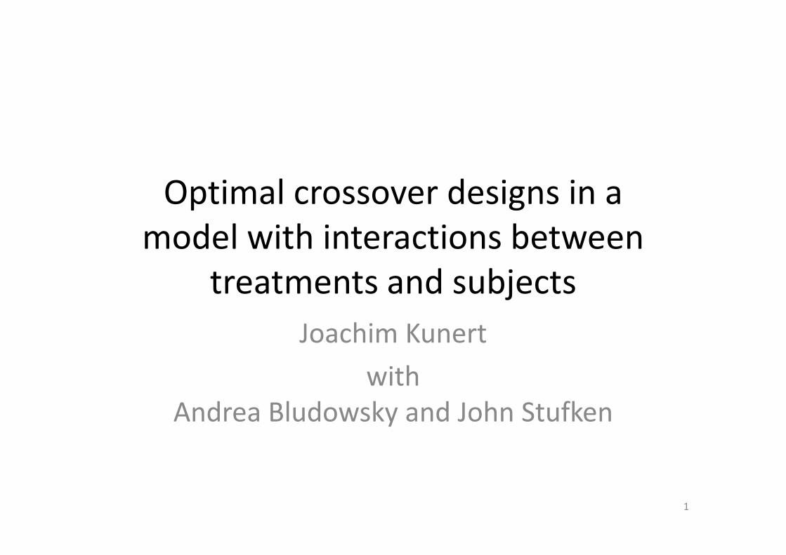
In crossover studies, each subject gets treated with a series of treatments,

one after the other.

2 4 3 1

2 1 4 3

1 2 3 4

2

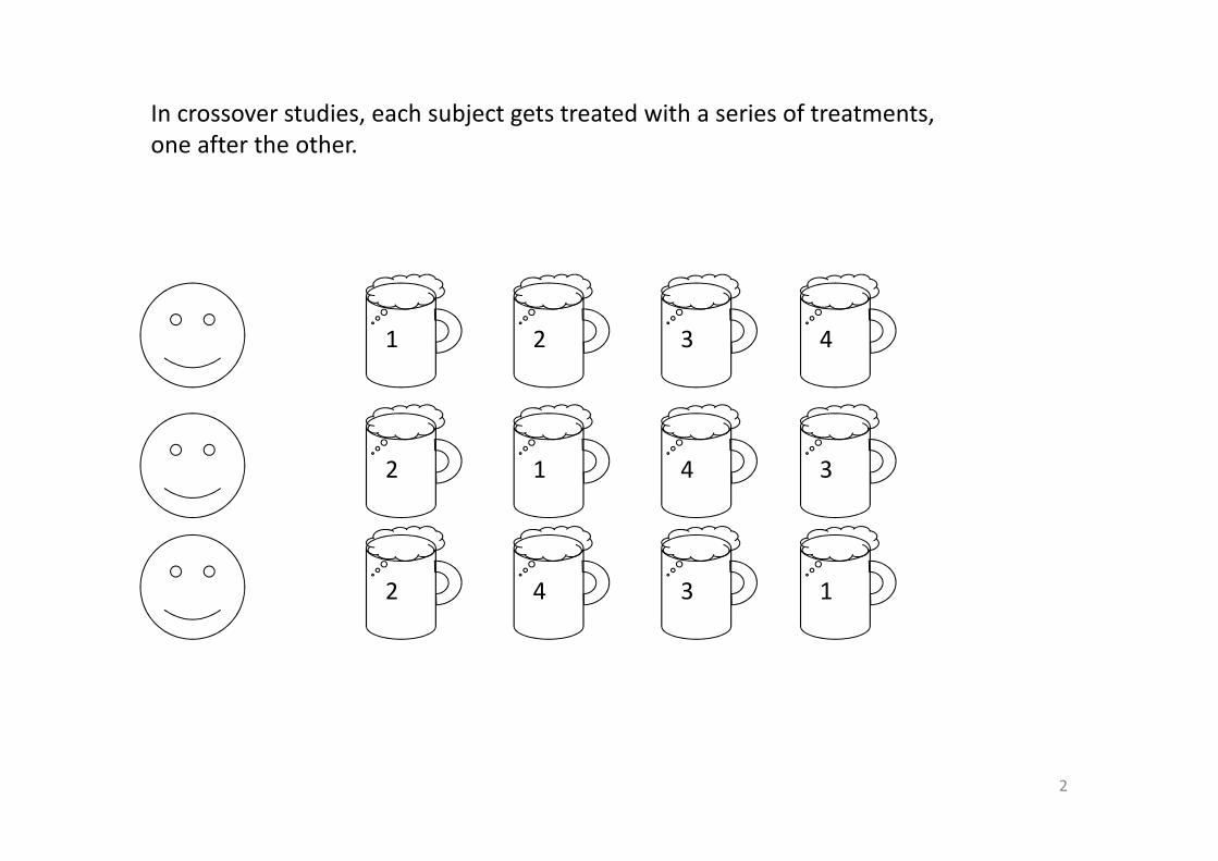
Most papers on optimal crossover designs consider a model with carryover

effects, such that

���� = �� �,� + � �,�� + �� + � + ��� ,

where the errors ���, … , ���, ���, … , ��� are i.i.d.

This model is often critizised because it implies that (neglecting carryover effects)

an experiment with � = 2 subjects and � = 100 observations per subject

provides as much information as

an experiment with � = 100 subjects and � = 2 observations per subject.

3

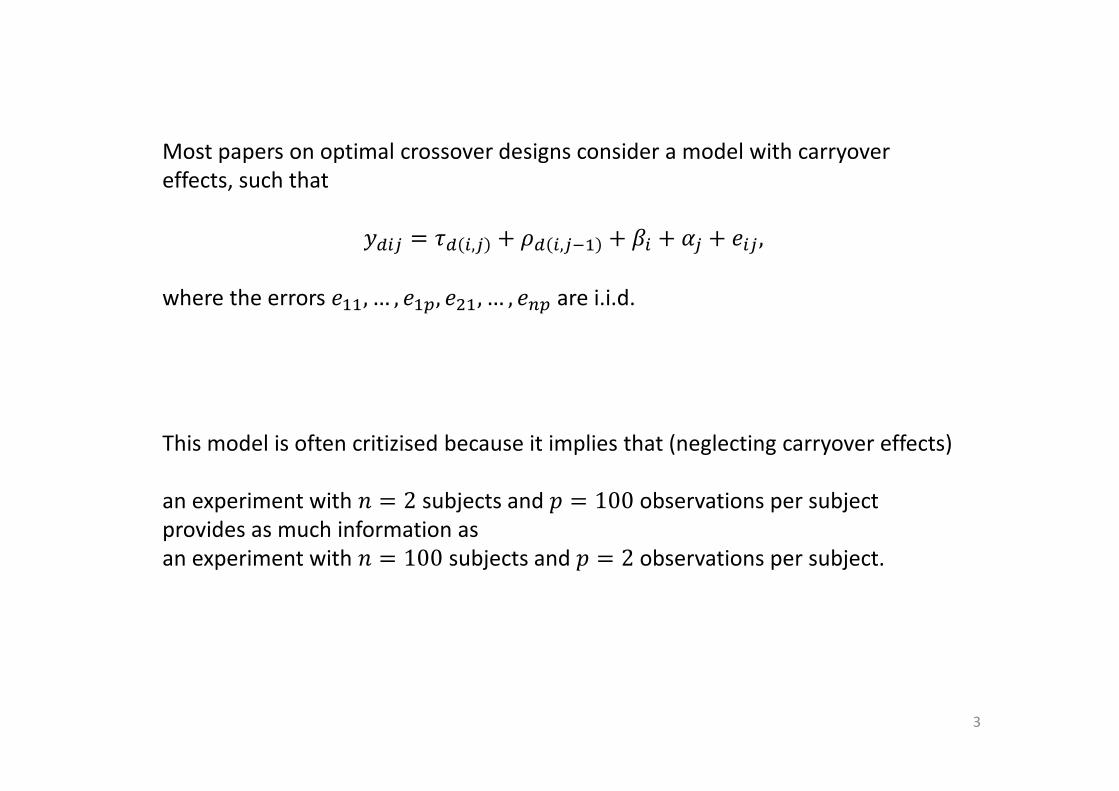
This clearly is not realistic :

For instance in preference studies,

one consumer comparing products A and B 50 times,

provides less information than 50 consumers comparing A and B just once.

Any consumer prefering A, will most likely prefer it all the time.

In consumer studies,

therefore often an interaction between product and consumer is modelled.

4

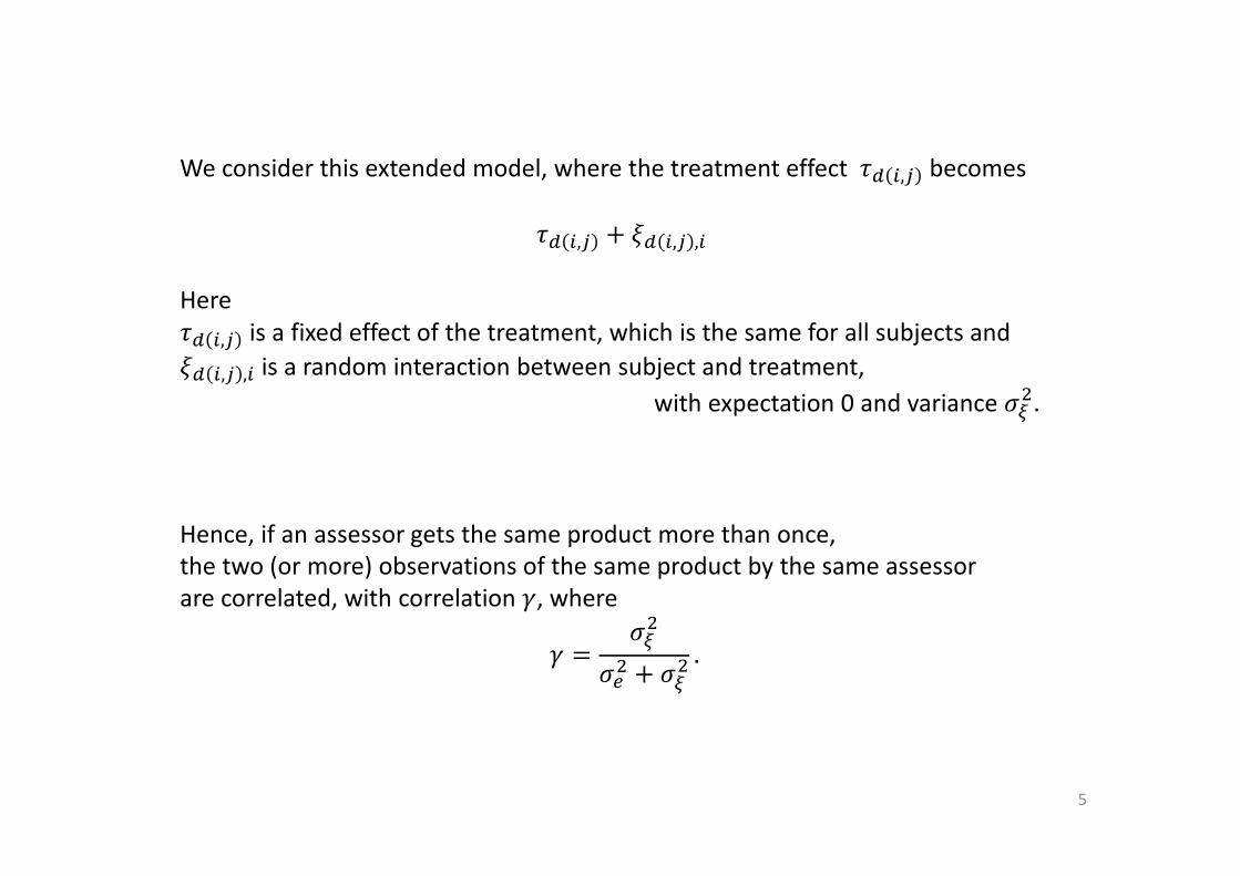
We consider this extended model, where the treatment effect �� �,� becomes

�� �,� + �� �,� ,�

Here

�� �,� is a fixed effect of the treatment, which is the same for all subjects and

�� �,� ,�is a random interaction between subject and treatment,

with expectation 0 and variance ���.

Hence, if an assessor gets the same product more than once,

the two (or more) observations of the same product by the same assessor

are correlated, with correlation �, where

� = ������ + ���

.

5

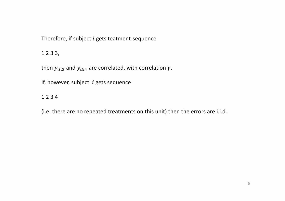
Therefore, if subject � gets teatment-sequence

1 2 3 3,

then ��� and ���! are correlated, with correlation �.

If, however, subject � gets sequence

1 2 3 4

(i.e. there are no repeated treatments on this unit) then the errors are i.i.d..

6

Although this model often is used in practice

(at least for preference studies),

there appear to be no published papers on optimal designs for this model.

Here is an attempt to fill this gap.

7

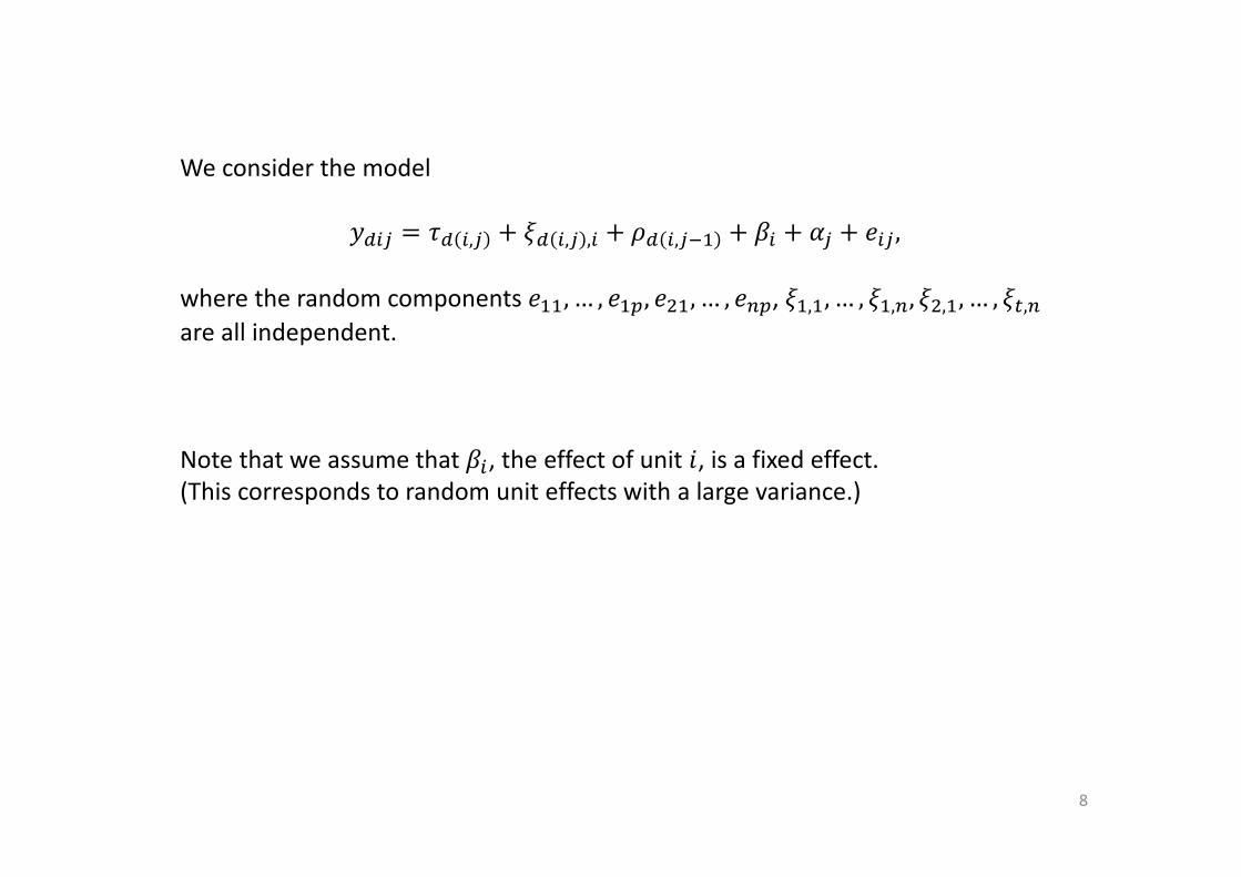
We consider the model

���� = �� �,� + �� �,� ,� + � �,�� + �� + � + ��� ,

where the random components ���, … , ���, ���, … , ���, ��,�, … , ��,�, ��,�, … , �",�are all independent.

Note that we assume that ��, the effect of unit �, is a fixed effect.

(This corresponds to random unit effects with a large variance.)

8

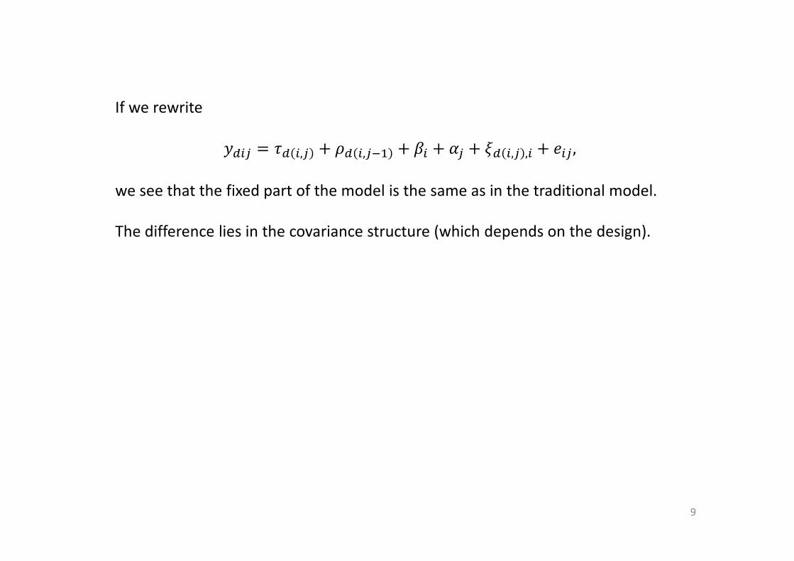
If we rewrite

���� = �� �,� + � �,�� + �� + � + �� �,� ,� + ��� ,

we see that the fixed part of the model is the same as in the traditional model.

The difference lies in the covariance structure (which depends on the design).

9

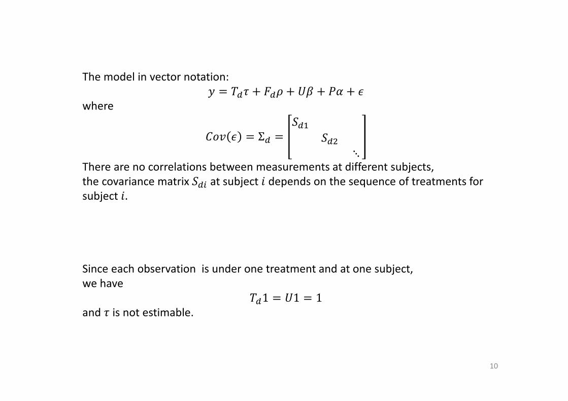
The model in vector notation:

� = #�� + $� + %� + & + 'where

()* ' = � =,��

,��⋱

There are no correlations between measurements at different subjects,

the covariance matrix ,�� at subject � depends on the sequence of treatments for

subject �.

Since each observation is under one treatment and at one subject,

we have

#�1 = %1 = 1and � is not estimable.

10

Kiefer (1975):

In a linear model

� = .� + /�� + �where .�1 ∈ �123�(/�)

consider

6, the unbiased estimate for 7 − �" 119 .

Information matrix:

(� = .�9:; /� .�.

This is the Moore-Penrose generalized inverse of ()*(�̂).

Note that (� has row- and column-sums zero.

11

Kiefer (1975):

If a design =∗ is such that

(i) (�∗ = 27" + @1"1"9(ii) AB2C�(�∗ = maxG∈H AB2C�(�

then =∗ is universally optimal over Δ.

12

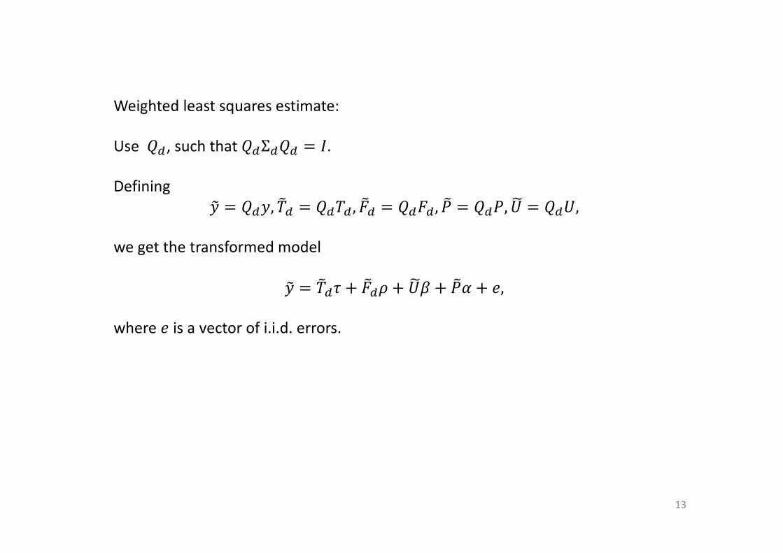
Weighted least squares estimate:

Use J�, such that J�Σ�J� = 7.

Defining

�K = J��, #L� = J�#� , $L� = J�$�, &L = J�&, %M = J�%,

we get the transformed model

�K = #L�� + $L� + %M� + &L + �,

where � is a vector of i.i.d. errors.

13

The information matrix is then

(� = #L�9:; $L�, %M, &L #L�,

which is not easy to handle.

To proceed, we need Kushner's method.

14

We consider approximate designs,

where the design-points are the possible sequences we might give to the subjects

and the weights are the proportions of subjects receiving these sequences.

Remember that we try to find a design =∗maximizing the trace of the information matrix.

For approximate designs, AB2C�(� = C��� − NOPQQNOQQ,

where C��� = AB2C�#L�9:; %M #L�,C��� = AB2C�#L�9:; %M $L�,

C��� = AB2C�$L�9:; %M $L�.

15

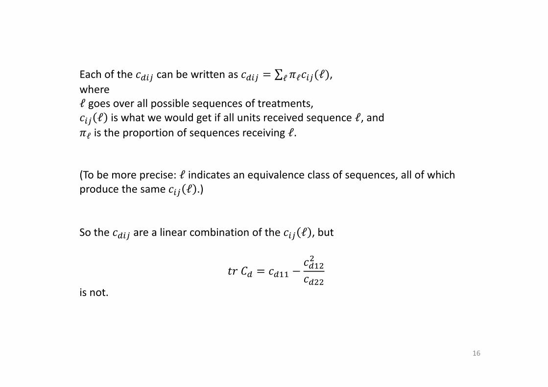
Each of the C��� can be written as C��� = ∑ SℓC��(ℓ), ℓwhere

ℓ goes over all possible sequences of treatments,

C�� ℓ is what we would get if all units received sequence ℓ, and

Sℓ is the proportion of sequences receiving ℓ.

(To be more precise: ℓ indicates an equivalence class of sequences, all of which

produce the same C�� ℓ .)

So the C��� are a linear combination of the C�� ℓ , but

AB(� = C��� −C����

C���is not.

16

Kushner (1997) observed that

AB(� = C��� −C����

C���is the minimum of

U� V = C��� + 2C���V + C���V�

and that

U� V =WSℓUℓ(V)ℓ

,

where

Uℓ V = C�� ℓ + 2C�� ℓ V + C�� ℓ V�

is the polynomial of the sequence class ℓ.

17

This implies that the U�(V) cannot be larger than the maximum of the Uℓ V

and minYU� V Z min

YmaxℓUℓ V .

18

19

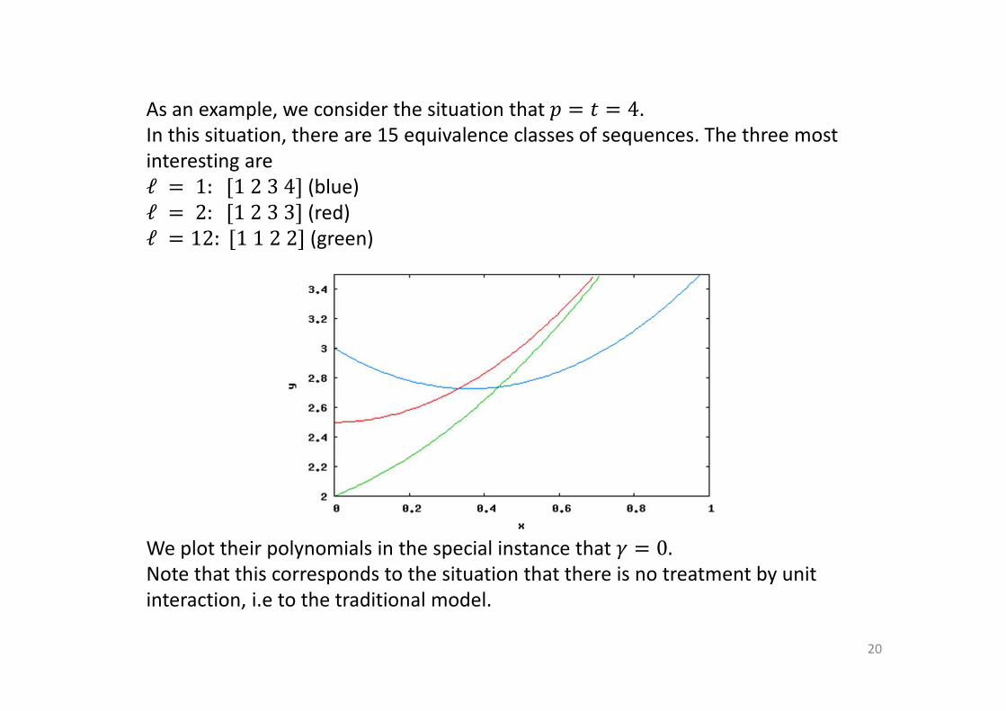
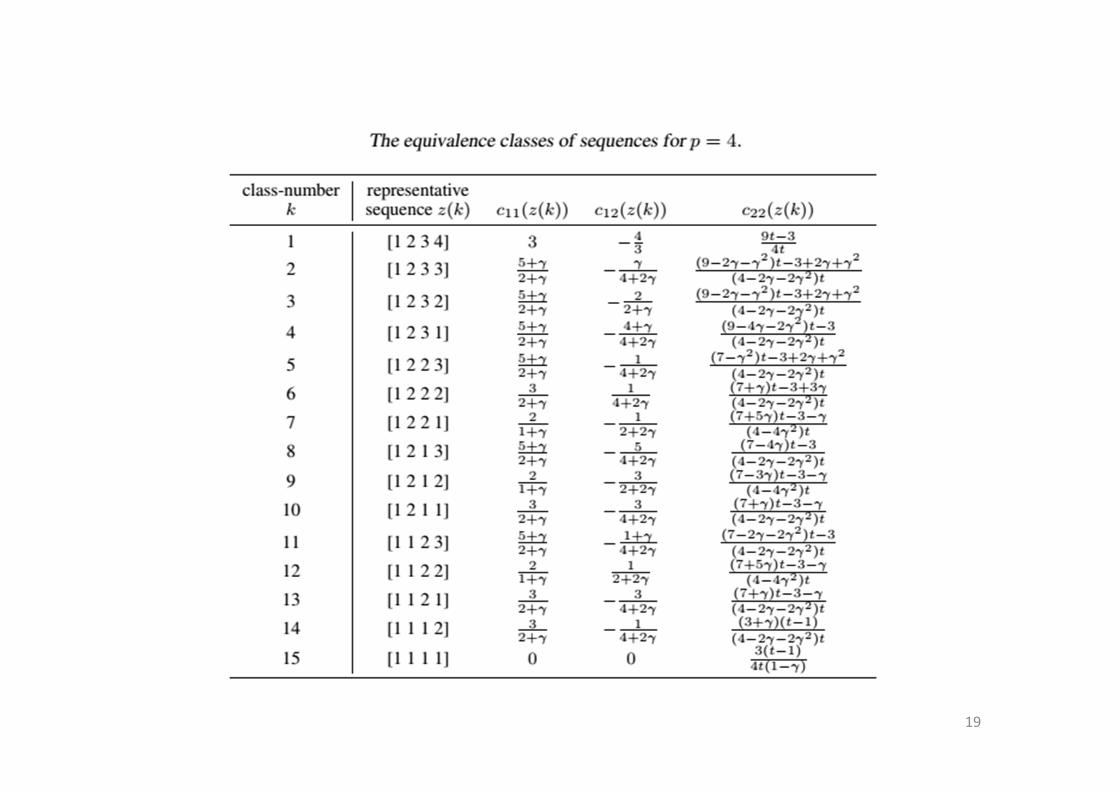
As an example, we consider the situation that � � A � 4.

In this situation, there are 15 equivalence classes of sequences. The three most

interesting are

ℓ � 1:]1234_ (blue)

ℓ � 2:]1233_ (red)

ℓ � 12:]1122_ (green)

We plot their polynomials in the special instance that � � 0.

Note that this corresponds to the situation that there is no treatment by unit

interaction, i.e to the traditional model.

20

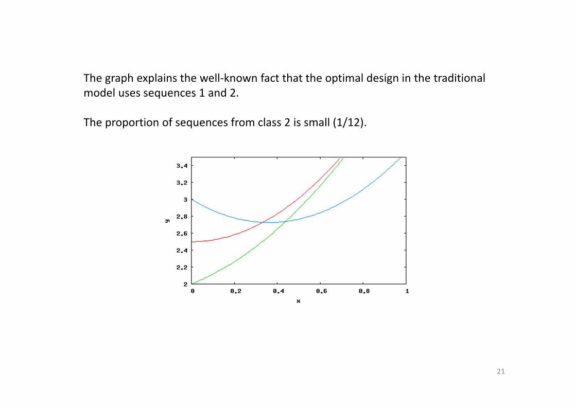
The graph explains the well-known fact that the optimal design in the traditional

model uses sequences 1 and 2.

The proportion of sequences from class 2 is small (1/12).

21

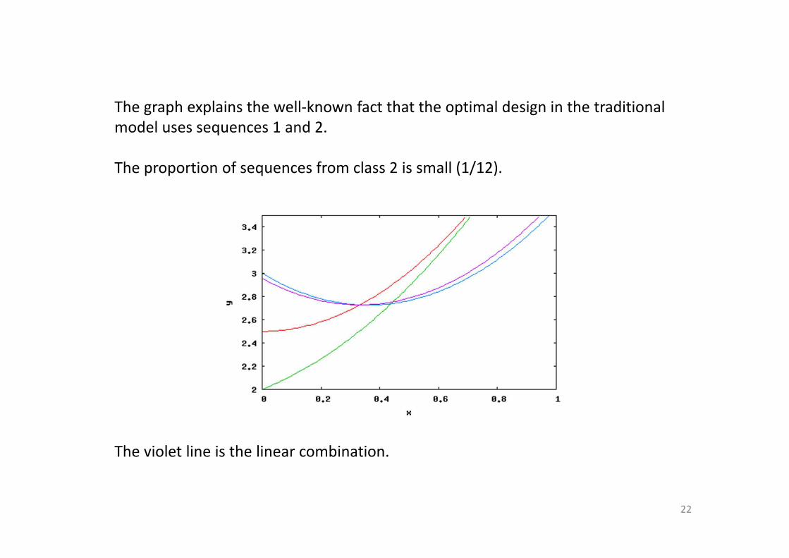
The graph explains the well-known fact that the optimal design in the traditional

model uses sequences 1 and 2.

The proportion of sequences from class 2 is small (1/12).

The violet line is the linear combination.

22

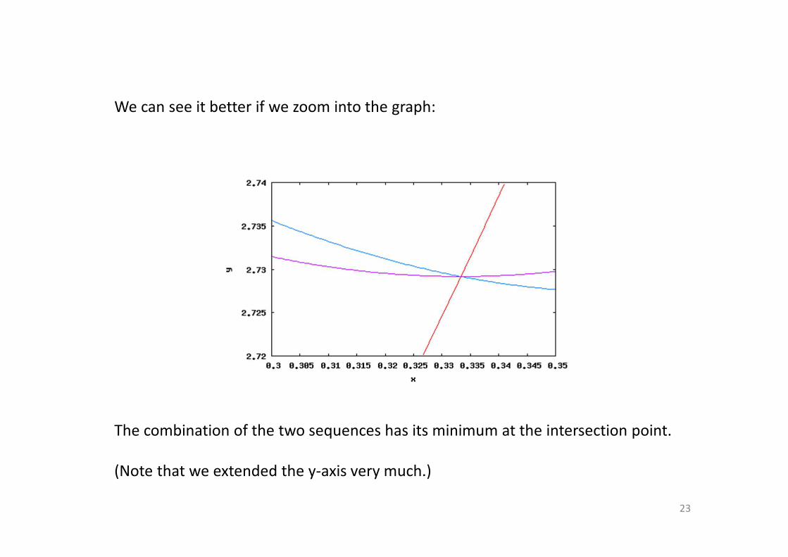
We can see it better if we zoom into the graph:

The combination of the two sequences has its minimum at the intersection point.

(Note that we extended the y-axis very much.)

23

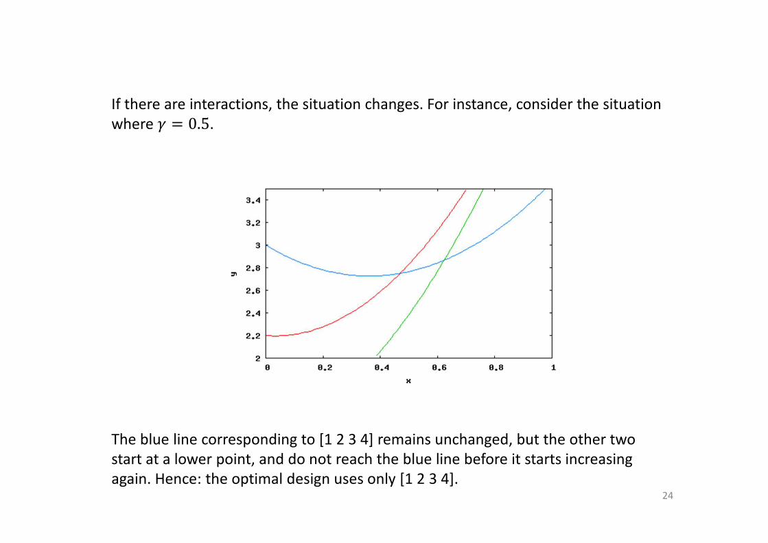
If there are interactions, the situation changes. For instance, consider the situation

where � � 0.5.

The blue line corresponding to [1 2 3 4] remains unchanged, but the other two

start at a lower point, and do not reach the blue line before it starts increasing

again. Hence: the optimal design uses only [1 2 3 4].24

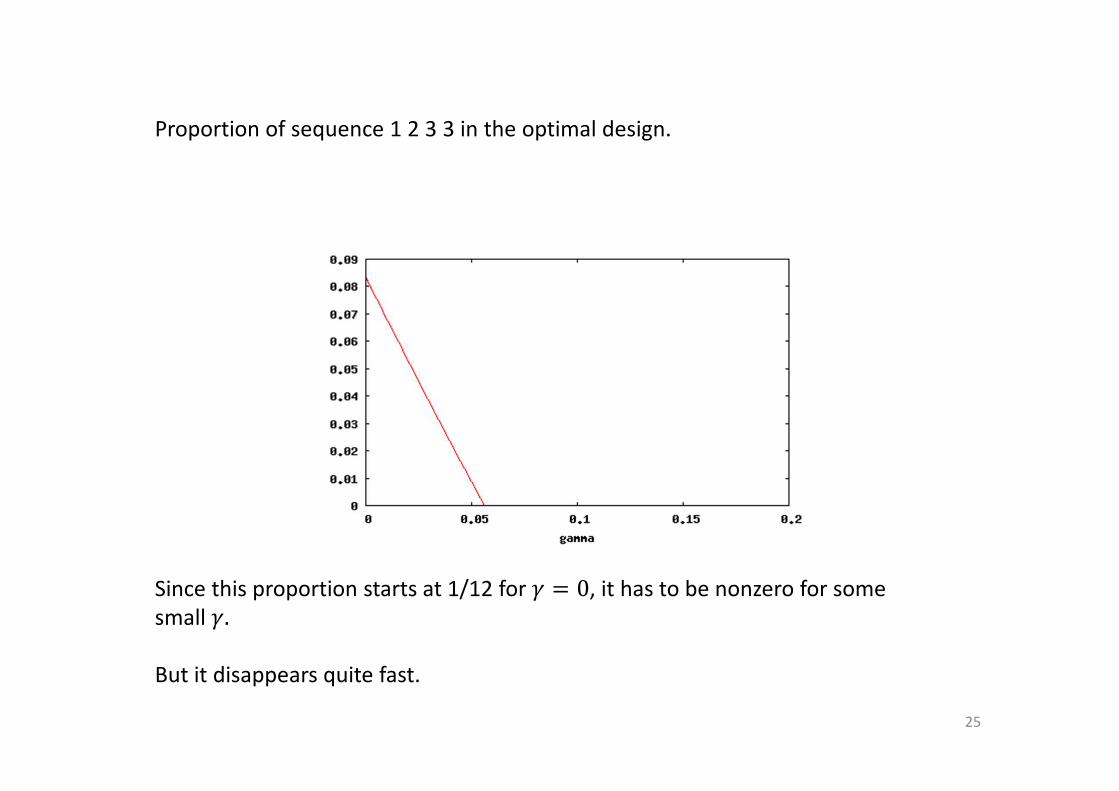
Proportion of sequence 1 2 3 3 in the optimal design.

Since this proportion starts at 1/12 for � � 0, it has to be nonzero for some

small �.

But it disappears quite fast.

25

This is exactly what I expected,

when I asked Andrea Bludowsky to work on this model for her thesis.

26

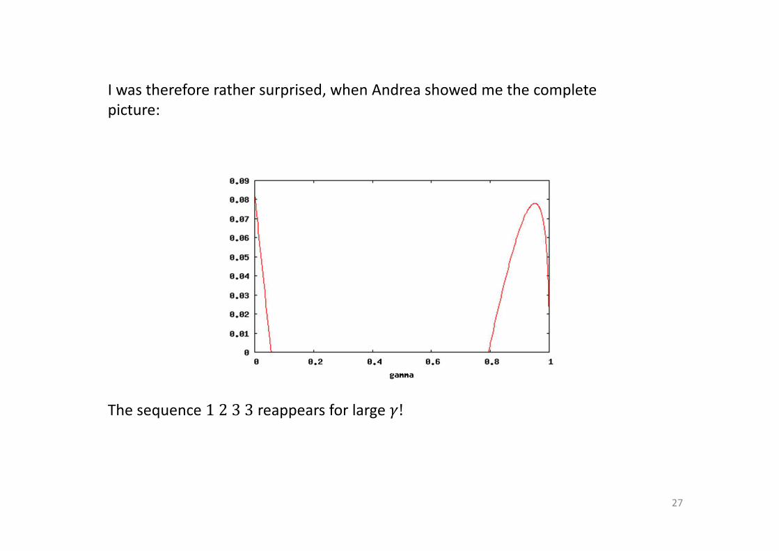
I was therefore rather surprised, when Andrea showed me the complete

picture:

The sequence 1233 reappears for large �!

27

We have considered the situation that � � 3, 4, 5 or 6.

For all the� that we considered,

if � is large, the optimal design uses pairs of identical treatments.

In fact, for larger �, even sequences like 123344 appear.

Is there a general stucture?

That is where we started at INI in 2011 .

28

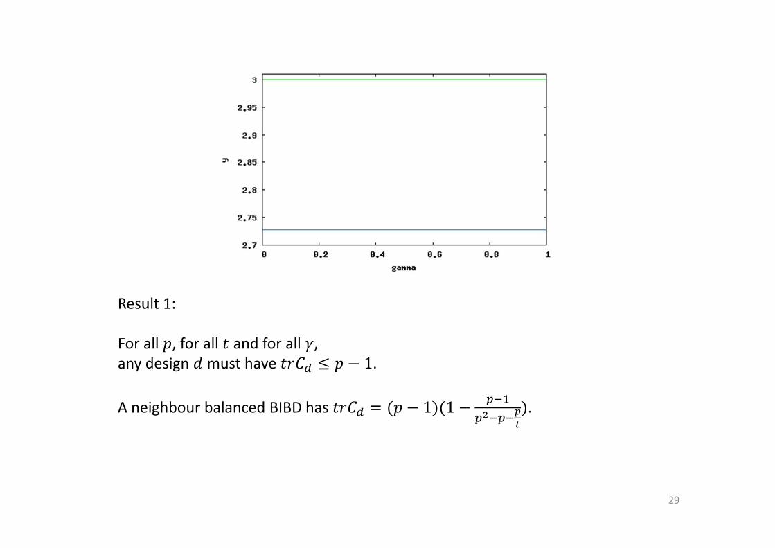
Result 1:

For all �, for all A and for all �,

any design = must have AB(� Z � 8 1.

A neighbour balanced BIBD has AB(� � 4� 8 1541 8��

�Q�e

f

5.

29

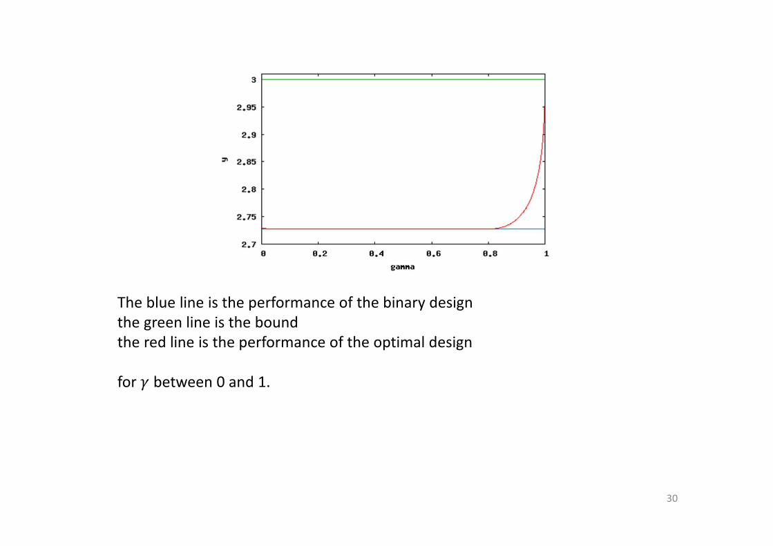
The blue line is the performance of the binary design

the green line is the bound

the red line is the performance of the optimal design

for � between 0 and 1.

30

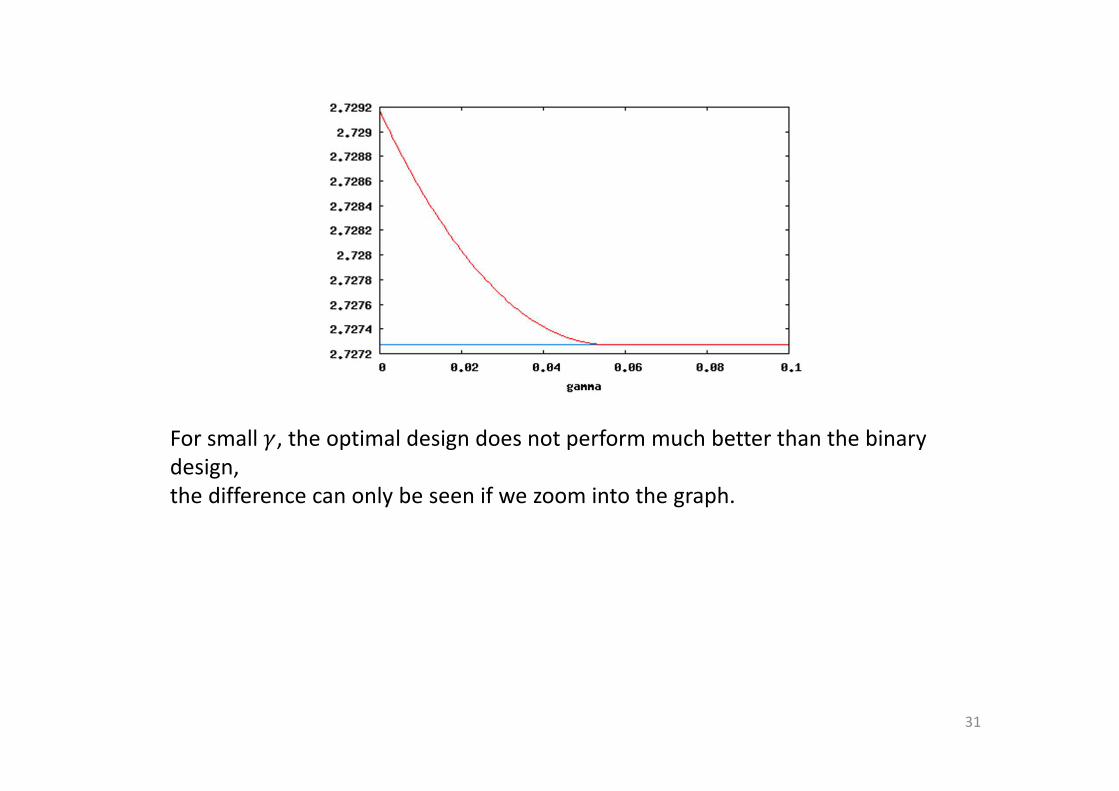
For small �, the optimal design does not perform much better than the binary

design,

the difference can only be seen if we zoom into the graph.

31

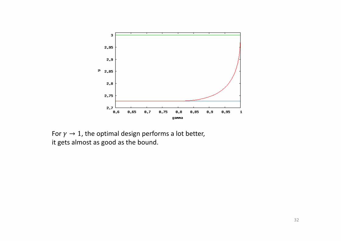
For � → 1, the optimal design performs a lot better,

it gets almost as good as the bound.

32

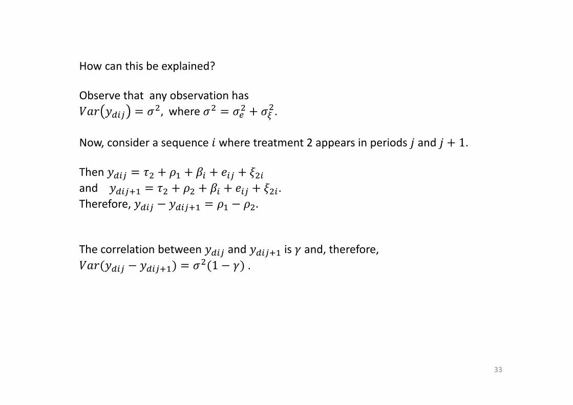
How can this be explained?

Observe that any observation has

h2B ���� � ��,where �� � ��� + ��

�.

Now, consider a sequence � where treatment 2 appears in periods i and i + 1.

Then ���� = �� + � + �� + ��� + ���and ����j� = �� + � + �� + ��� + ���.Therefore, ���� − ����j� = � − �.

The correlation between ���� and ����j� is � and, therefore,

h2B(���� − ����j�) = ��(1 − �).

33

Therefore, in the limit as � → 1, a small proportion of sequences with identical

pairs allows to estimate the carryover effects with variance almost zero.

The other sequences can then be used to estimate the direct effects with the

same precision as if there were no carryover effects.

Result 2:

For all �, for all A. If � → ∞,

then for the optimal design =∗ we get AB(�∗ → � − 1.

34

References:

Kiefer, J. (1975): Construction and optimality of generalized Youden designs. In:

A Survey of Statistical Design and Linear Models (J.N. Srivastava, ed.), North

Holland, Amsterdam

Kushner, H.B. (1997): Optimal Repeated Measurements Designs: The Linear

Optimality Equations. Annals of Statistics 25, 2328 - 2344

Bludowsky, A. (2009): Optimal Crossover Designs with interactions between

treatments and units. Thesis, TU Dortmund

Bludowsky, A., Kunert, J., Stufken,J. (2015): Optimal designs for the carryover

model with random interactions between subjects and treatments.

Australian and New Zealand Journal of Statistics, to appear

35