Performance of Adaptive Optics

Systems

Don Gavel

UCSC

Center for Adaptive Optics

Summer School

August, 2008

Outline

• Performance Measures

• The construction of error budgets

• AO error contributors

• AO system simulation

• Gathering performance data on real AO systems

• Performance results: Lick AO

Performance measures

• Wavefront error

E x t ~ ,

2 2

• Strehl Ratio

SPSF

PSF

max

, ~

0 00

Strehl ratio

Lick 3m Telescope Keck 10m Telescope

The Strehl is related to the wavefront variance

through Marechal’s approximation

SPSF

PSF Nx e d x

D x

P

0 0

0 0

1

0

0

1 2 2

2

,

,

exp

~

~

• Valid approximation for small

~

300 dof

80 dof

Exp - 2~

~2 2 (radians)

Str

ehl R

atio

• Extended region of validity

for AO-corrected wavefronts

Resolution

The Rayleigh criterion: in a diffraction-limited optical system, two

point sources are separately distinguishable at a separation ~l/d

In AO systems with a Strehl

>~0.15, the FWHM of the

corrected image is ~l/d

F. Rodier introduced the

concept of “Strehl-resolution” =

width you have to enclose to

get the same energy as in the

FHWM of the ideal PSF

Image contrast

• Contrast = ratio of halo to core “surface” brightness

• Integration time required to detect a faint object in the halo

is proportional to (contrast)-2

Keck AO example at l=2m

Distance from the primary star, arcseconds

Co

ntr

as

t R

ati

o

The SNR-optimal slit-width transitions to l/d

when the Strehl gets > 0.1

Energy in a spectrograph slit

D.L.

unc

Additional measures

• Field performance

• PSF stability

7 layer model atmosphere with r0 =

15.6 cm and 0 = 3.1 arcsec

Optimize on disk

DM at 0 km DMs at 0,10 km

DMs at 0,5,10 km

Field Performance of Multi-conjugate AO

• Fitting error (DM)

• Control error (sample rate)

• Measurement error (Hartmann sensor)

• Isoplanatic error (field angle)

• Calibration error

• Laser guide-star specfic errors: cone effect, guide-star elongation

AO system error contributors

~2 2 2 2 2 2 2 DM BW SNR iso cal cone

To some approximation, we can add these terms in quadrature

DM fitting error

DM DM

P

S k F kd d k2 2

S k r k 0 023 0

5 3 11 3.

The DM corrects the wavefront up to

a spatial frequency of 1/(actuator

spacing)

Example spatial filtering function

d

Kolmogorov turbulence

mDM d r2

0

5 3

F kd( )

kd

kdF

kd()

x d/

zx

DM

DM fitting error

Influence Function Spatial Frequency Response

The fitting error coefficient, m, depends on the

type of deformable mirror

Segmented mirror

Square segment, m=0.174

Hexagonal segment, m=0.116

d

d

Continuous face sheet DM: m=0.3

• Segmented mirrors requre 3 (piston, tip, tilt)

actuators per segment

• Rewriting the fitting error in terms of number of

actuators, Na shows its more economical to

use a continuous mirror:

mDM Na aD N r2

0

5 3

mNa

0 355

0 339

0 221

.

.

.

square

hex

contin

Control bandwidth error

Example temporal filtering function

f fc

F f fc

BW cS f F f f df2

S f r v f 2 6 0

5 3 8 3. /

BW g cf f25 3

f f

f f

c

c

2

21

The control loop corrects the wavefront up to a temporal

frequency of f fc s 10

“Greenwood frequency” -

depends on wind velocity, r0,

etc., but simply defined here as

the control frequency where the

bandwidth term=1 radian2

Wavefront measurement error

l

SNRx SNR

2

2 0

1d

I d d

I d

x y x y

y y

( , )

( , )

Spot-size factor

(units: angle on the sky)

Control loop

averaging factor

Reconstructor

noise propagator

SNR SNR SNRx y

2 2 2

Isoplanatic error

h

00

r

h

iso

2

0

5 3

Turbulent layer

Light from

science object

Light from

guide star

• If the guide star is not the science object...

Isoplanatic angle:

DM at 0 km DMs at 0,10 km

DMs at 0,5,10 km

Anisoplanatic error can be controlled by MCAO

Residual error is the “generalized

anisoplanatism” = (/m )5/3

(Tokovinin&LeLouarn, 2000)

Laser guidestar specific errors

• Cone effect

Z

h

dZ

hr0 02

e.g…. h=4 km, r0=10cm > d0=4.5m

Laser Guidestar at finite altitude

cone d d2

0

5 3

The laser guide star has a larger apparent size than a

natural star

• The wavefront measurement error is increased accordingly

Spot size (arcsec)

DL (d=25cm) 0.4

star (r0=11cm) 0.94

LGS 2.16

Laser

StarStar

StarStar Laser

LGS

Star

Radius, arcsec

Enci

rcle

d e

ner

gy

Lick laser data, from Nov. 1999

Laser guide star

Natural star

Optimizing the error budget

• In the design, select d (subaperture size =~ DM actuator

spacing) to trade between DM fitting term and

measurement term. This will set the NGS limiting

magnitude, or “sky coverage”. It will also set the

“optimized wavelength” of the AO system: l:r0(l)=d.

• For a laser guide star system, trade measurement error

for laser power. Select the optimum d for the predicted

LGS brightness. Brighter lasers (and more actuators) get

to shorter wavelengths.

• On-line tuning:

• Select a frame rate that will best trade off

measurement and bandwidth terms

• Select a natural guide star to trade off brightness

(measuement error) for field angle (isoplanatic error)

Contoller bandwidth, fc

Su

ba

pe

rture

siz

e,

d

increasing

brightness

Simultaneous

Solution

Gu

ide

sta

r m

agn

itu

de, m

vSubaperture size, d

Rms wavefront error, nm

Optimizing the error budget

Simulating an AO system

• Heirarchy of modeling

• Scaling laws

• “Analytic” models (usually working in transform space)

• Monte-carlo wave-optic simulation

• Tools:

• Kolmogorov screen generator

• Wavefront propagation code

• DM model, WFS model

• Imaging model

Monte-carlo Simulation of an AO system

Generate a guide star

Near-field propagation

Generate a phase screen, add to

wavefront’s phase

Continue to propagate

Generate another phase screen,

add to wavefront’s phase...

Multiply by the aperture function

Subtract the DM’s phase

Run through the WFS model

Run through the controller model

Apply the DM actuator response

model

Image residual

wavefront

wind

Gathering performance data on a real AO system

• Telemetry:

• Wavefront sensor data (slopes, intensities) >

controller’s rejection curve, bandwidth error term,

measurement error term

• DM actuator commands > simutaneous r0

• Image data:

• Open loop > r0

• Closed loop > Strehl

Error Budget Summary – Key Terms in an

Astronomical AO Error Budget

r0 (Fried seeing parameter) Histogram

0

10

20

30

40

50

0 5 10 15 20 25 30

r0, cm

# o

f o

cc

ura

nc

es

median r0 = 10 cm

Seasonal Variation of Seeing

02468

101214161820222426

1 2 3 4 5 6 7 8 9 10 11 12

Month

r0,

cm

(2000-2002)

Histogram of Wind Speeds

0

50

100

150

200

0 5 10 15 20 25 30 35 40 45 50

Wind Speed, m/sec

# o

f o

ccu

ran

ces

Greenwood Frequency Histogram

0

5

10

15

20

0 5 10 15 20 25

fg, Hz

# o

f o

ccu

ran

ces

Lick seeing statistics

D. Gavel, E. Gates, C. Max, S. Olivier, B. Bauman, D. Pennington, B. Macintosh, J. Patience, C. Brown, P. Danforth, R.

Hurd, S. Severson, J. Lloyd, Recent Science and Engineering Results with the Laser Guidestar Adaptive Optics System at

Lick Observatory, Proc SPIE, 4839, pp. 354-359 (2003).

Performance vs Guide Star Brightness

0

0.1

0.2

0.3

0.4

0.5

0.6

0.7

0.8

10 100 1000 10000

Brightness, ph/subap/ms

Str

eh

l BrG

Ks

H

Performance vs Greenwood Frequency

0

0.1

0.2

0.3

0.4

0.5

0.6

0.7

0.8

0 10 20 30 40

fg, Hz

Str

eh

l

BrG

Ks

Ks-dim

H

Performance vs Seeing

0

0.1

0.2

0.3

0.4

0.5

0.6

0.7

0.8

0 5 10 15 20 25

r0, cm

Str

eh

l

BrG

Ks

Ks-dim

H

Lick AO System: performance statistics

LGS Performance

0

0.1

0.2

0.3

0.4

0.5

0.6

0.7

0.8

0 5 10 15 20 25

r0

Str

eh

l Ks Nov01

BrG Oct00

Ks Oct00

Strehl Histogram BrG Filter

0

1

2

3

4

5

6

0

0.1

0.2

0.3

0.4

0.5

0.6

0.7

0.8

Strehl

# o

f o

ccu

ran

ces

BrG

Strehl Histogram Ks Filter

0

1

2

3

4

5

6

7

0

0.1

0.2

0.3

0.4

0.5

0.6

0.7

0.8

Strehl

# o

f o

ccu

ran

ces

Ks-Dim

Ks

Lick AO System: performance statistics 2001-2002

Lick AO System: On-line Performance Analysis

Fill in the seeing and other system parameters in the green boxes and read the Strehl in the blue box

Lick Error Budget r0 0.15 m

radians@.55 nm Strehl@lambdaObs v-wind 10 m/s

counts 100 photo-electrons Fitting 2.405180443 210.538 0.70 tau0 0.015 s

read noise 6 electrons Bandwidth 0.838952777 73.43791 0.96 fg 9 Hz

spot FWHM 2 arcsec SNR 1.223671374 107.1143 0.91 mu 1

spot sigma 1.442695 arcsec Calibration 1.583226455 138.5881 0.85 d 0.43 m

pixel size 2 arcsec Aniso 0 0 1.00 fs 100 Hz

crosstalk 0.2 arcsec Strehl 283.5481 0.52 fc 10 Hz

centroider quad FWHM open loop 0.75630429 arcsec at lambdaObs lambda 550 nm

SNR 6.401844 note: need to load math package in Excel (erf) to connect this to calculations belowObserved 0.35 lambdaObs 2200 nm

theta 0 arcsec Unaccounted 2.510864718 219.7891 0.67 calibration 0.85 Strehl (BrG)

Quad Cell SNR 4.125565 theta0 6 sec

• The spreadsheet errorbudget.xls can help diagnose the sources of

Strel loss and aid with on-line AO system parameter adjustments

• Other on-line metrics at the operator interface, based on AO system

telemetry data analysis:

• Seeing r0

• Wind velocity

• Temporal power spectrum of turbulence

• Control loop rejection curves

k-8/3 spectrum

wind

clearing

time scale

noise floor

Lick AO Telemetry Data Analysis Pipeline

Hartmann

slopes

Actuator

voltages

Subaperture

intensities

Raw

Hartmann

images

Average over

illuminated

subaps

Frame

rate

Determine

guidestar

intensity

Verify proper background

subtraction & photometry

Determine

SNR

Generate phase

spectra

Frame rate

Generate controller

rejection curve

Fit effective

loop gain

Derive

Hartmann spot

size

Electronic

loop gain

Determine

wavefront

measurement

error

Control params

Generate tilt

spectraAccount for tilt

in phase spectra

Account for

sensor noise in

phase spectra

Calculate

Greenwood

frequency

Calculate

integrated temporal

power rejection

Compare to

Greenwood

model

Open-loop

images

Pre-calibrate rms

actuator voltage to

micron ratio

Calculate rms

phase correction

by DM

Determine r0 from

rms phase

correctionCalculate fitting

error

SNR

BW

DM

Control

matrix

Actuator spacing

Compute the

compensator

function

Determine

sensor noise

Measure Hartmann spot

size of internal source

Compute noise

averaging

factor

HK = I

Modeling the effect of noise in closed loop

Correcting the closed loop residual phase

spectrum for the effects of noise

f

fDM

en

e

e H H ncor cl f

H fH f

H fcl

ol

ol

1

H f H fH f

cor cl

ol

11

1

Closed-loop transfer function: low-pass “Correction” transfer function: high-pass

e H ncor f

f n 0

S H S H S

S H S H S

e cor cl n

e cl cl n

2 2

2 2

f

f

S S H He e cor cl

2 2

=============================================

Lick 3m error budget

/duck5/lickdata/sep00/lgs6data/sep08/cent_07

Saturday 09/09/00 23:03:44 PDT

---------------------------------------------

Fitting Error (sigmaDM) 117.827 nm

d = 42.8571 cm

r0Hv = 13.6763 cm

---------------------------------------------

Servo Error (sigma_BW) 85.8510 nm

fc = 45.9980 Hz

fgHv = 28.5525 Hz

fs = 500 Hz

---------------------------------------------

Measurement Error (sigma2phase) 81.9109 nm

SNR = 45.7691

control loop averaging factor = 0.452526

spotSizeFactor = 0.882759 arcsec

---------------------------------------------

TOTAL: 167.221 nm

=============================================

=============================================

Lick 3m error budget

/duck5/lickdata/may00/lgs6/may21/cent_03

5/22/00, 5:09 UT

---------------------------------------------

Fitting Error (sigmaDM) 122.912 nm

d = 42.8571 cm

r0Hv = 13.0001 cm

---------------------------------------------

Servo Error (sigma_BW) 174.682 nm

fc = 30.5027 Hz

fgHv = 40.2416 Hz

fs = 500.000 Hz

---------------------------------------------

Measurement Error (sigma2phase) 15.2976 nm

SNR = 100.543

control loop averaging factor = 0.257468

spotSizeFactor = 1.23077 arcsec

---------------------------------------------

TOTAL: 214.138 nm

=============================================

Measuring AO Performance

Julian C. Christou and Donald Gavel

UCO/Lick Observatory

CfAO 2006

10 here w0

0

pk

pk S

p

h

rp

rhS

• Other Approaches besides Strehl Ratio

• Image Sharpness (originally described by Muller and Buffington,

1974)

S1 - Size of PSF

S3 - Normalised peak value – directly related to Strehl Ratio

2

2

1

i

i

h

hS

pk

3

ih

hS

Advantage – independent of knowing peak location and

value. - Can be applied to extended sources.

Disadvantage – The numerator is contaminated by an additive

noise term n2.

)(

)(

3

3pkpk

pS

hS

p

p

h

hSR

ii

Disadvantage – sensitive to measurement of peak location and value.

Advantage – No noise bias

1. Palomar pupil geometry: primary mirror diameter of 4.88m and a central obscuration of 1.8m. No secondary supports modelled.

2. H-band (1.65 microns) with different levels of AO correction.

Ideal PSF

• Sharpness criteria

compared with residual

wavefront error from

the simulations.

• S1 has a steeper slope

for smaller rms phases.

S1 – -0.45 nm-1

S3 – -0.30 nm-1

(nm)

Relationship between S1, S3

and the Strehl Ratio.

S1 and S3 values generated

from noise-free simulations

as part of the CfAO Strehl

study.

Both S1 and S3 are

normalised to those of the

ideal PSF.

The effect of constant noise

is shown on S1.

Variation in NGS PSF quality from the Lick AO system (all at 2 microns)

Ideal PSF

• Sharpness (normalised

S1) compared with Strehl

ratio for NGS Lick AO

data.

• Data obtained with

different SNR, observing

conditions, nights.

• Dashed line obtained

hueristically from the

noiseless simulations..

Departure from simulations could be due to either overestimating S1 (e.g. presence

of noise) or underestimating Strehl ratio (not accurately locating the peak). Further

analysis on noisy simulations needed.

Accuracy of system performance measurements can be obtained from SR and S1.

• Science Targets- Basic Astronomy; stellar classification; stellar motion – orbits

• AO Performance - Isoplanatic Issues – on-axis vs. off-axis performance

- Isoplanatic angle - o

• Analysis Performance

- Measurement of Photometry and Astrometry

• Lick Observatory Data- NGS

- 0.5" Separations 12"

CrB m Cas Cas

70 Oph Del WDS 00310+2809

Lick NGS Data

12" 5"

1"

9"

7" 0.5"-7"

• Binary stars permit direct measurement of anisoplanatism by

comparing the PSFs.

• An effective measure of anisoplanatism is the fall off of the Strehl

ratio of the off-axis source compared to the on-axis source.

where is the binary separation

oaxis-on

axis-off exp

SR

SR

• Del (sep = 9.22 arcseconds) – ratio = 0.76 ± 0.04 o= 20.1" ± 2.1"

• 70 Oph (sep = 4.79 arcseconds) – ratio = 0.84 ± 0.04 o = 14.3" ± 2.5"

Summary of Binary Strehl Ratio Measurements

• Strehl ratio changes vary similarly for both components.

• Strehl ratio is quite variable for a set of observations ( seconds - minutes)

up to changes of 20%.

• Differential Strehl ratio also varies – relative position on the detector?

• Isoplanatic angle (as determined from differential Strehl ratio) also varies

with 15" o 30" with some results implying minutes!

• Analysis Techniques

- Iterative Blind (myopic) deconvolution (Christou-CfAO)

- Parametric Blind Deconvolution (PSF Modelling) (Drummond-

AFRL)

• Astrometry and Photometry

(on following pages)

Summary of Astrometry and Photometry

• Astrometry between the two techniques shows good agreement ( 0.001")

• Differential Photometry is in general good agreement ( 0.02 mag) with a

few exceptions.

- CrB (J = 0.5)

- m Cas (J = 0.4; Br = 0.2)

- Cas Aa (J = 0.2; Ks = 0.2)

- Cas Ac (H = 0.15)

Christou, J.C., Drummond, J.D., Measurements of Binary Stars, Including Two New

Discoveries, with the Lick Observatory Adaptive Optics System, The Astronomical Journal,

Volume 131, Issue 6, pp. 3100-3108.

Astronomical AO System Data

Analysis

Julian Christou (UCSC)

Szymon Gladysz (NUI)

Gladysz, S., Christou, J., Redfern, M., Characterization of the Lick adaptive optics point

spread function, SPIE Proc., 6272, June, 2006

• Data sets obtained at Lick almost monthly between July 2005 and

Feb 2006.

• IRCAL fastsub mode (“freeze” images)

- texp = 22ms and 57ms

- Duty cycle ~ texp + 30ms

• field size of 4.864 4.864 arcseconds (64 64 pixels)

• Target objects: mv~ 6-8

• Typically 10 sets of data each of 1000 frames - 104 total frames

High Speed PSF Measurements

Long Term PSF Stability

Ideal PSF Fiber 1 (Sep-2005) Fiber 2 (Oct-2005) 12-Oct-2005

Reference Change

18-Aug-2005 18-Aug-2005 25-Jul-2005 25-Jul-2005

28-Aug-2004 29-Aug-2004 27-Aug-2004

78%

20 Nov 2005

80%

13 Oct 2005

75%

17 Sep 2005

Lick AO Fiber Source

• Stable structure in atmospheric-free PSF

• Strehl Ratios typically 75% -- 82%

PSF Structure• Fiber Source no better than ~ 80% Strehl ratio.

– What’s the best we can do - 90-95%?

• Strong high-order Residual Aberration limiting performance.

– Relatively stable over minutes hours days months years!

– No significant change with change of DM references

– Where is this from?

• DM flatness

• Unsensed aberrations in main path

• Non-common path errors

• Incorrect SH References

• Obtain Wavefront map from Phase Retrieval/Diversity measurements.

– Typically the image is “sharpened” on the sky

• Relative peak value metric - other metrics e.g. S1

• First 10 Zernike terms and increasing to 20.

– Use mirror modes?

• Important to understand for PSF Reconstruction algorithms.

– We can deal with the atmosphere but can we deal with the system …?

Lick NGS Strehl Stability (10000 frames 22-57ms/frame)

Christou (UCSC), Gladysz (NUI)

• Distribution of Strehl ratios (for relative stable performance) all show a similar

non-gaussian behaviour.

• Similar distributions seen in data from Palomar, Keck and AEOS

Strehl Ratio Distributions

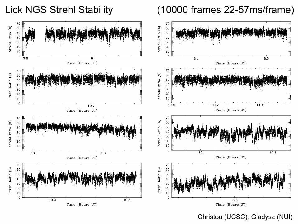
PDF Models

x = S x = 100 / (100 - S) x = ln(100 - S)

PDF Models

Implication is that the instantaneous Strehl ratio has an underlying Gaussian

distribution: of r0 !• Using Hudgin and Marachel approximations produces a distribution of Strehl

ratios similar to that measured, i.e. skewed to a low Strehl ratio tail.

• Need to obtain simultaneous r0 and S measurements.

• Speckle noise dominating.

PSF Calibration and Quantitative Analysis

• The complicated nature of the AO PSF makes quantitative analysis

problematic.

– How well does deconvolution preserve

astrometry and photometry?

i Cas

AMOS 9-9-05

Separation of the components of CrB

Sub-pixel peaks located by Fourier interpolation

o Six separate measurements of a binary star on different days on

different positions on the IRCAL detector.

o Separation depends upon location on detector

o Precision for each location ~ 2 mas (= 0.03 pixels = 1.5% l/D)

o Separation dispersion ~ 50 mas

Julian C. Christou, Austin Roorda, and David R. Williams, Deconvolution of adaptive

optics retinal images, J. Opt. Soc. Am. A 21, 1393-1401 (2004)

xxxxxx ndfhg

Deconvolution of final images, using data from the

wavefront sensing

Object NoisePSFImage

ffff NFHG Fourier Transform:

framemulti

*2

framemulti

* NHFHGH

Then (in the Fourier domain):

0

= +

Then solve for object F …

ffFfF

AO Performance Measurement

• AO performance-hitters (intro to error budget)

• AO modeling and simulation

• AO performance metrics

– Sharpness and anisoplanatism measures from the

AO corrected science image

– Spectral analysis of telemetry from the AO system

(wavefront sensor and deformable mirror signals)

• Astronomical AO data analysis

• Vision science AO data analysis

Summary conclusion

CfAO Summer School, 2008