Physics 111: College Physics Laboratory

Laboratory Manual

Montana State University-Billings

Fall 2006

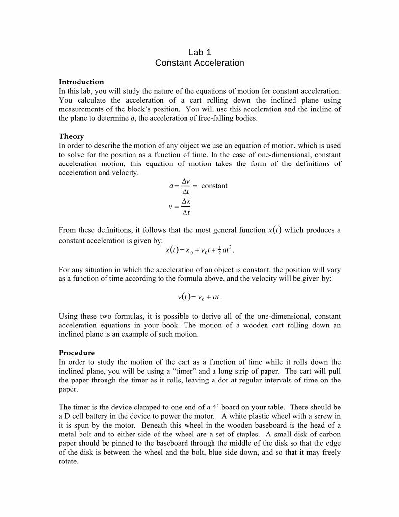
Lab 1 Constant Acceleration

Introduction In this lab, you will study the nature of the equations of motion for constant acceleration. You calculate the acceleration of a cart rolling down the inclined plane using measurements of the block’s position. You will use this acceleration and the incline of the plane to determine g, the acceleration of free-falling bodies. Theory In order to describe the motion of any object we use an equation of motion, which is used to solve for the position as a function of time. In the case of one-dimensional, constant acceleration motion, this equation of motion takes the form of the definitions of acceleration and velocity.

a = ΔvΔt

= constant

v =ΔxΔt

From these definitions, it follows that the most general function x t( ) which produces a constant acceleration is given by:

x t( ) = x 0 + v0t + 12 at2 .

For any situation in which the acceleration of an object is constant, the position will vary as a function of time according to the formula above, and the velocity will be given by:

v t( )= v0 + at . Using these two formulas, it is possible to derive all of the one-dimensional, constant acceleration equations in your book. The motion of a wooden cart rolling down an inclined plane is an example of such motion. Procedure In order to study the motion of the cart as a function of time while it rolls down the inclined plane, you will be using a “timer” and a long strip of paper. The cart will pull the paper through the timer as it rolls, leaving a dot at regular intervals of time on the paper. The timer is the device clamped to one end of a 4’ board on your table. There should be a D cell battery in the device to power the motor. A white plastic wheel with a screw in it is spun by the motor. Beneath this wheel in the wooden baseboard is the head of a metal bolt and to either side of the wheel are a set of staples. A small disk of carbon paper should be pinned to the baseboard through the middle of the disk so that the edge of the disk is between the wheel and the bolt, blue side down, and so that it may freely rotate.

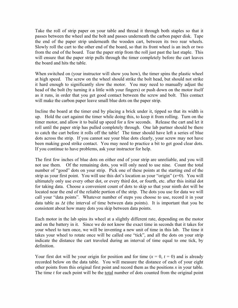
Take the roll of strip paper on your table and thread it through both staples so that it passes between the wheel and the bolt and passes underneath the carbon paper disk. Tape the end of the paper strip underneath the wooden cart, between its two rear wheels. Slowly roll the cart to the other end of the board, so that its front wheel is an inch or two from the end of the board. Tear the paper strip from the roll just past the last staple. This will ensure that the paper strip pulls through the timer completely before the cart leaves the board and hits the table. When switched on (your instructor will show you how), the timer spins the plastic wheel at high speed. The screw on the wheel should strike the bolt head, but should not strike it hard enough to significantly slow the motor. You may need to manually adjust the head of the bolt (by turning it a little with your fingers) or push down on the motor itself as it runs, in order that you get good contact between the screw and bolt. This contact will make the carbon paper leave small blue dots on the paper strip. Incline the board at the timer end by placing a brick under it, tipped so that its width is up. Hold the cart against the timer while doing this, to keep it from rolling. Turn on the timer motor, and allow it to build up speed for a few seconds. Release the cart and let it roll until the paper strip has pulled completely through. One lab partner should be there to catch the cart before it rolls off the table! The timer should have left a series of blue dots across the strip. If you cannot see your blue dots clearly, your screw may not have been making good strike contact. You may need to practice a bit to get good clear dots. If you continue to have problems, ask your instructor for help. The first few inches of blue dots on either end of your strip are unreliable, and you will not use them. Of the remaining dots, you will only need to use nine. Count the total number of “good” dots on your strip. Pick one of these points at the starting end of the strip as your first point. You will use this dot’s location as your “origin” (x=0). You will ultimately only use every other dot, or every third dot, or fourth, etc. after this initial dot for taking data. Choose a convenient count of dots to skip so that your ninth dot will be located near the end of the reliable portion of the strip. The dots you use for data we will call your “data points”. Whatever number of steps you choose to use, record it in your data table as Δt (the interval of time between data points). It is important that you be consistent about how many dots you skip between data points. Each motor in the lab spins its wheel at a slightly different rate, depending on the motor and on the battery in it. Since we do not know the exact time in seconds that it takes for your wheel to turn once, we will be inventing a new unit of time in this lab. The time it takes your wheel to rotate once will be called one “tick”, and all the dots on your strip indicate the distance the cart traveled during an interval of time equal to one tick, by definition. Your first dot will be your origin for position and for time (x = 0, t = 0) and is already recorded below on the data table. You will measure the distance of each of your eight other points from this original first point and record them as the positions x in your table. The time t for each point will be the total number of dots counted from the original point

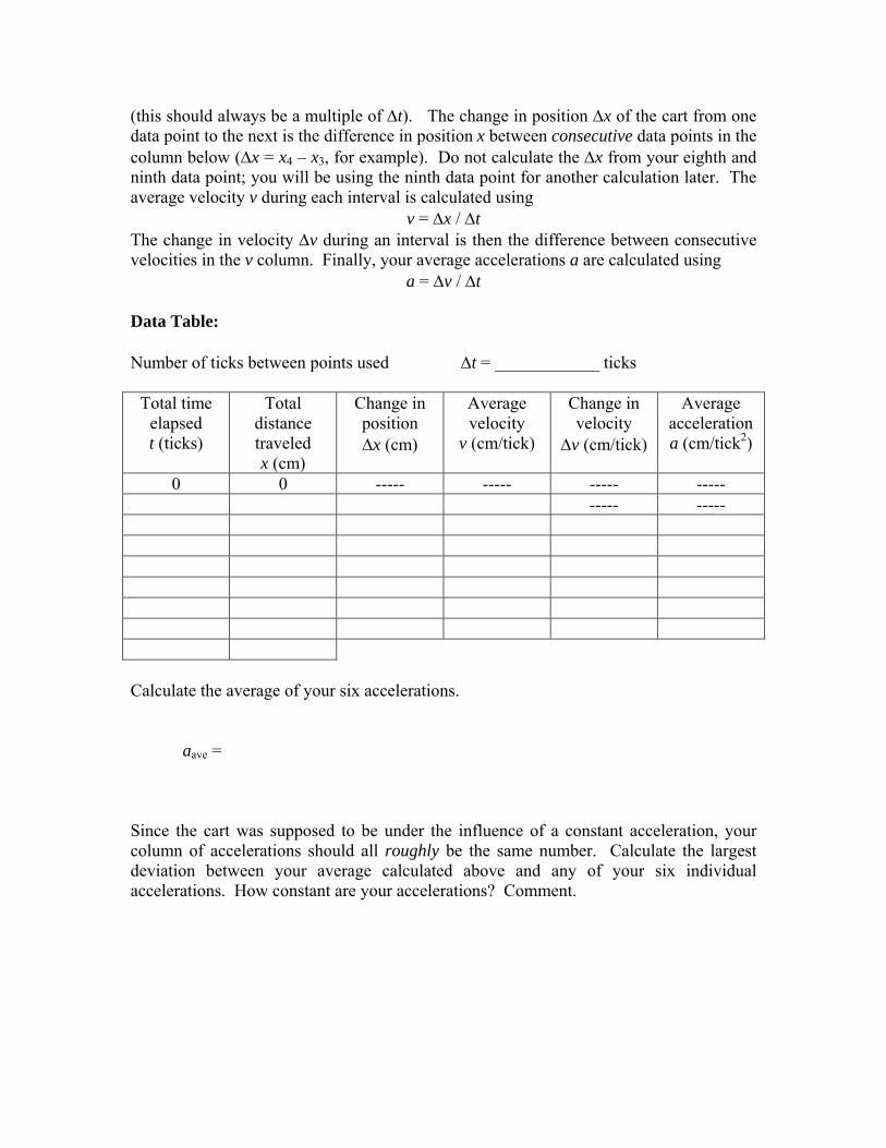
(this should always be a multiple of Δt). The change in position Δx of the cart from one data point to the next is the difference in position x between consecutive data points in the column below (Δx = x4 – x3, for example). Do not calculate the Δx from your eighth and ninth data point; you will be using the ninth data point for another calculation later. The average velocity v during each interval is calculated using

v = Δx / Δt The change in velocity Δv during an interval is then the difference between consecutive velocities in the v column. Finally, your average accelerations a are calculated using

a = Δv / Δt Data Table: Number of ticks between points used Δt = ____________ ticks

Total time elapsed t (ticks)

Total distance traveled x (cm)

Change in position Δx (cm)

Average velocity

v (cm/tick)

Change in velocity

Δv (cm/tick)

Average acceleration a (cm/tick2)

0 0 ----- ----- ----- ----- ----- ----- Calculate the average of your six accelerations. aave = Since the cart was supposed to be under the influence of a constant acceleration, your column of accelerations should all roughly be the same number. Calculate the largest deviation between your average calculated above and any of your six individual accelerations. How constant are your accelerations? Comment.

Make a graph of your seven velocities vs. time. For greater accuracy, plot each point on the time axis at a point in the middle of the time interval for which that average velocity was calculated. For example, if velocity v3 was calculated using the cart’s position at times t = 12 ticks and t = 16 ticks, it should be plotted on your graph at time t = 14 ticks. Draw the best-fit line to your velocities. Calculate the slope of the line and the y-intercept of the line. The slope should be the constant acceleration a of your cart, and the y-intercept should be the initial velocity v0 of the cart at time t = 0 ticks. How well do your data points fit a straight line? Comment: Using the two quantities you determined from the graph, predict where your ninth data point should have been with the formula:

x t( ) = x 0 + v0t + 12 at2

For your initial position, use x0 = 0. Plug in the time t of your ninth point and solve: x9 = Now, calculate a percent error between your experimentally measured position for the ninth point and the theoretically predicated position,

th

thex

MMM −

=err % =

For reference in future labs, Mth always represents a theoretical calculation and Mex an experimental measurement of some quantity. Use the percent error to compare how close the two numbers are to each other. Comment:

Lab 2 Projectile Motion

In this lab, we will use the equations for projectile motion to determine the initial velocity of a ball fired from a spring-loaded gun, which we will then use to predict the range of the ball when the gun is elevated. The gun is placed on a lab table so that it will fire a ball horizontally off of the table. From our knowledge of projectile motion, we know that it will follow a parabolic path to the floor. If we know the height of the table and the range of the ball, we can work the equations for projectile motion backwards to find the initial velocity of the ball as it leaves the gun. If these equations hold true, then we should be able to predict where the ball will land if the gun is elevated so that the initial velocity is not horizontal. Thus, this experiment is going to test the validity of the vector equation:

r t( ) = ro + vo t + 12 at 2.

Procedure: Set the gun up on the edge of a lab table and fire the gun once to get an idea for the range of the ball. Next, tape a piece of paper to the floor in the approximate location of where the ball landed. Fire the gun again. If the ball lands on the paper, it will leave a mark. Do this five times without moving the gun or the paper. Measure the horizontal distance from the end of the gun to the marks on the paper and take the average of the five readings. Record this value and the largest deviation which your individual measurements make from the average: Rav =

ΔR =

100%av

RRΔ

× =

Measure and record the height of the gun off of the floor: h = Knowing that the ball has no initial vertical component of velocity, we can calculate the time required for it to drop from the height h. Show this calculation and record your answer: t =

Knowing the range of the ball and the time that it spends in the air, we can calculate the initial velocity. Show this calculation and record your answer: v o =

At this point, we now know the initial velocity of the ball as it leaves the gun. If the front of the gun is elevated so that it makes an angle θ with the horizontal, we have a generic projectile motion problem in which the height (h), the magnitude of the initial velocity ( v o ), and the angle (θ) are known. We can now calculate the expected range.

To find the angle θ, measure the height that the front of the gun is elevated by, and the distance between the feet of the gun. The angle can be found using trigonometry from these two measurements. Measure h and θ for the new set-up: h = θ = Using the v o from the first part, calculate the expected range and record this value:

Rex =

Next, tape the paper in the appropriate region where you expect the ball to land and fire the gun five times. Find the average value and record the largest deviation which your individual measurements make from the average: Rav = ∆R =

100%av

RRΔ

× =

Is this deviation comparable to the one found in the first part? (If not, go back and do it again).

Calculate the percent error between your predicted range Rex and your experimental range Rav. Does Rex fall within the range given by R ± ΔR ? Comment on how accurate your

prediction was:

Lab 3 Inclined Plane

Whenever a body slides along another body, a resisting force appears which is called the force of friction. This is a very important force and serves many useful purposes. A person could not walk without it, or a car could not propel itself along a road without the friction between the tires and the road. On the other hand, friction is sometimes very wasteful. It reduces the efficiency of machines, work must be done to overcome it, and this work is wasted as heat. The purpose of this experiment is to study the laws of sliding friction and to determine the coefficient of friction between two surfaces. THEORY: Friction is the resisting force encountered when one surface slides, or tends to slide, over another; this force acts along the tangent to the surfaces in contact. The size of this frictional force depends only on the nature of the materials in contact (their roughness or smoothness) and on the normal force, it does not depend upon the area of contact. It is found experimentally that the force of friction is directly proportional to the normal force. The constant of proportionality is called the coefficient of friction. The coefficient of friction (μ) is defined to be the ratio of the force of friction to the total normal force between the surfaces. Thus:

nFf=μ or nFf μ= .

Note that the value of μ depends upon the surfaces in contact and therefore is different for different substances. Thus, the coefficient of friction is given for substance A on substance B -- for example, μ = 0.19 for pine on particle board. We will determine the coefficient of friction for two particular substances using two different methods, and then we will show that μ is independent of the normal force. PROCEDURE: If a body is placed on an inclined plane which is not frictionless, then the angle at which the body will slide down the plane at constant velocity (i.e. with no acceleration) is related to the coefficient of friction by ( )θμ tan= where θ is called the "angle of repose".

Draw a free-body diagram and prove that this is true using Newton's second law: Take the frictional surface and place the brick on it. Begin tilting the surface while tapping the brick. When you reach the angle of repose, the brick will begin sliding down the surface at constant velocity. Record this angle, and calculate the coefficient of friction: θ = μ = If a body is placed on a flat surface which is not frictionless and connected to a hanging weight by a pulley and string, then the body will move at a constant velocity when the frictional force is balanced by the tension in the string. Draw a free-body diagram of this situation and, using Newton's second law, show that the frictional force must be equal to the hanging weight if the acceleration is to be zero: Take the frictional surface and lay it level. Connect the hanging weight to the brick via the pulley. Increase the hanging weight by adding mass to it while tapping the brick. When the hanging weight is equal to the frictional force, the brick will begin to slide down the frictional surface at constant velocity. Record this weight (which is also

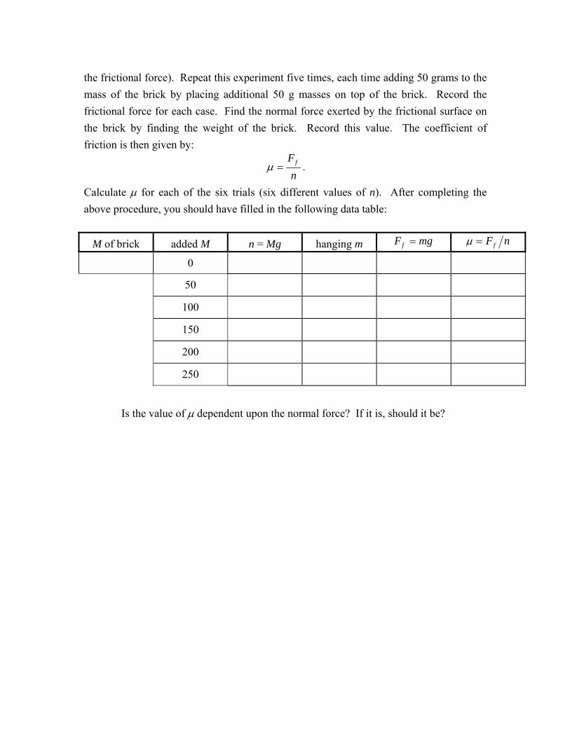
the frictional force). Repeat this experiment five times, each time adding 50 grams to the mass of the brick by placing additional 50 g masses on top of the brick. Record the frictional force for each case. Find the normal force exerted by the frictional surface on the brick by finding the weight of the brick. Record this value. The coefficient of friction is then given by:

nFf=μ .

Calculate μ for each of the six trials (six different values of n). After completing the above procedure, you should have filled in the following data table:

M of brick added M n = Mg hanging m mgFf = nFf=μ

0

50

100

150

200

250

Is the value of μ dependent upon the normal force? If it is, should it be?

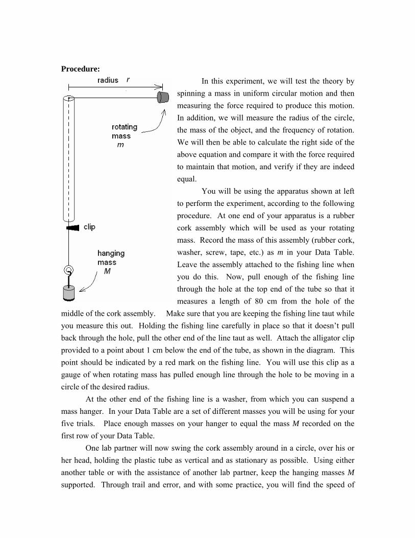
Lab 4 Uniform Circular Motion

In order for a body to move in a circle or travel along a circular path, there must be a net outside force applied on that body. Newton's first law requires this. In addition, using a bit of geometry, we can show that this applied force must constantly change its direction so as to always point towards the center of the circle. Such a force is called a centripetal force. Whenever you see anything moving in a circle, you may rest assured that somewhere there is an agent supplying the necessary centripetal force to allow for such "unnatural" motion. (Remember, straight line motion is "natural" motion.) It might be helpful for you to analyze a few cases of circular motion to be sure that you can find the source of the force responsible for this peculiar motion. The purpose of this experiment is to study uniform circular motion and to compare the measured value of the centripetal force with the value one would expect from theoretical considerations. Theory: If a body is moving with uniform speed in a circle of constant radius r, it is said to be moving in uniform circular motion. Even though the speed is constant, the velocity is continually changing, since the direction of the motion is constantly changing. Thus such a body is accelerating. Recall from class that the direction of the acceleration is always toward the center of the circle and the magnitude of the acceleration is given by

rva

2

=

The speed of the body is v, and r is the radius of the path. Note: The direction of the acceleration is continually changing as the body moves around the circle. We know from Newton's second law that accelerations don't just happen all by themselves. There must be a net outside force acting on the object in order for it to accelerate. Furthermore, if the object has a mass of m and experiences an acceleration a, then the strength of the force must be numerically equal to m times a. Because this force is directed inward towards the center of the circle it is sometimes called a centripetal force. Hence, the size of the necessary force for an object of mass m to move in a circle of radius r with a speed v is given by:

rmvFc

2

=

Procedure:

In this experiment, we will test the theory by spinning a mass in uniform circular motion and then measuring the force required to produce this motion. In addition, we will measure the radius of the circle, the mass of the object, and the frequency of rotation. We will then be able to calculate the right side of the above equation and compare it with the force required to maintain that motion, and verify if they are indeed equal. You will be using the apparatus shown at left to perform the experiment, according to the following procedure. At one end of your apparatus is a rubber cork assembly which will be used as your rotating mass. Record the mass of this assembly (rubber cork, washer, screw, tape, etc.) as m in your Data Table. Leave the assembly attached to the fishing line when you do this. Now, pull enough of the fishing line through the hole at the top end of the tube so that it measures a length of 80 cm from the hole of the

middle of the cork assembly. Make sure that you are keeping the fishing line taut while you measure this out. Holding the fishing line carefully in place so that it doesn’t pull back through the hole, pull the other end of the line taut as well. Attach the alligator clip provided to a point about 1 cm below the end of the tube, as shown in the diagram. This point should be indicated by a red mark on the fishing line. You will use this clip as a gauge of when rotating mass has pulled enough line through the hole to be moving in a circle of the desired radius. At the other end of the fishing line is a washer, from which you can suspend a mass hanger. In your Data Table are a set of different masses you will be using for your five trials. Place enough masses on your hanger to equal the mass M recorded on the first row of your Data Table. One lab partner will now swing the cork assembly around in a circle, over his or her head, holding the plastic tube as vertical and as stationary as possible. Using either another table or with the assistance of another lab partner, keep the hanging masses M supported. Through trail and error, and with some practice, you will find the speed of

circular motion necessary to hold the hanging mass M suspended only by the circular motion of the mass m at a radius of t. The tension in the fishing line provides the centripetal force Fc for mass m, and will be equal to the weight Mg of the hanging masses when those masses are suspended unsupported. Using a stop watch, time how long it takes for the cork to complete 10 full revolutions. Record this time on the Data Table. Now, repeat the experiments four more times for each mass M listed on the Table. Complete the calculations in the Data Table. In the last column, indicate the percent difference between the centripetal force calculated in the third column and that calculated in the seventh column:

%100error %

2

×−

=c

c

Fr

mvF

Data: Mass of cork assembly m = Radius of motion r = 80 cm = 0.80 m Circumference of motion (in meters) 2πr =

Trial Hanging mass

M (kg)

Centripetal force

Fc = Mg

Time for 10

revolutions 10 t× (s)

Time for 1 revolution

t (s)

Speed v of mass m (m/s)

Centripetal force mv2/r

% error

1 0.150

2 0.250

3 0.300

4 0.350

5 0.450

On the basis of your percent errors calculated above, has the theoretical formula

rmvFc

2

= been confirmed?

Lab 5 The Simple Pendulum

Introduction and Objectives: The laboratory is a place for the investigation of physical phenomena and principles. Originally, scientists studied physical phenomena in the laboratory in the hope that they might discover relationships and principles involved in phenomena. This might be called the “trial and error” method. Today, investigations are carried out using the Scientific Method. This approach states that no theory, model, or description of nature is tenable unless the results it predicts are in accord with experimental observations. We will use the scientific method to determine the acceleration due to gravity g, using a simple pendulum.

Procedure: A pendulum consists of a “bob” (a mass) attached to a string that is fastened to a point in such a manner that it can swing freely, or oscillate, in a plane about that point. For a simple pendulum, it is assumed that all of the mass of the bob is concentrated at one point, i.e. the center of mass of the bob.

1. Set up a pendulum using the bob provided and a length of string of about 75 cm.

2. Measure the period of oscillation (the time required for the bob to complete one cycle of its swing) as a function of the angle through which the pendulum is displaced. A protractor is used to measure this angle. The period is determined by timing 10 oscillations with a stopwatch and then dividing by 10.

Angle Time for 10 oscillations (sec) Time for 1 oscillation (T)

(sec)

10°

20°

30°

40°

50°

In the space below, write a statement concerning the period T with the size of the angle. Is there a consistent relationship?

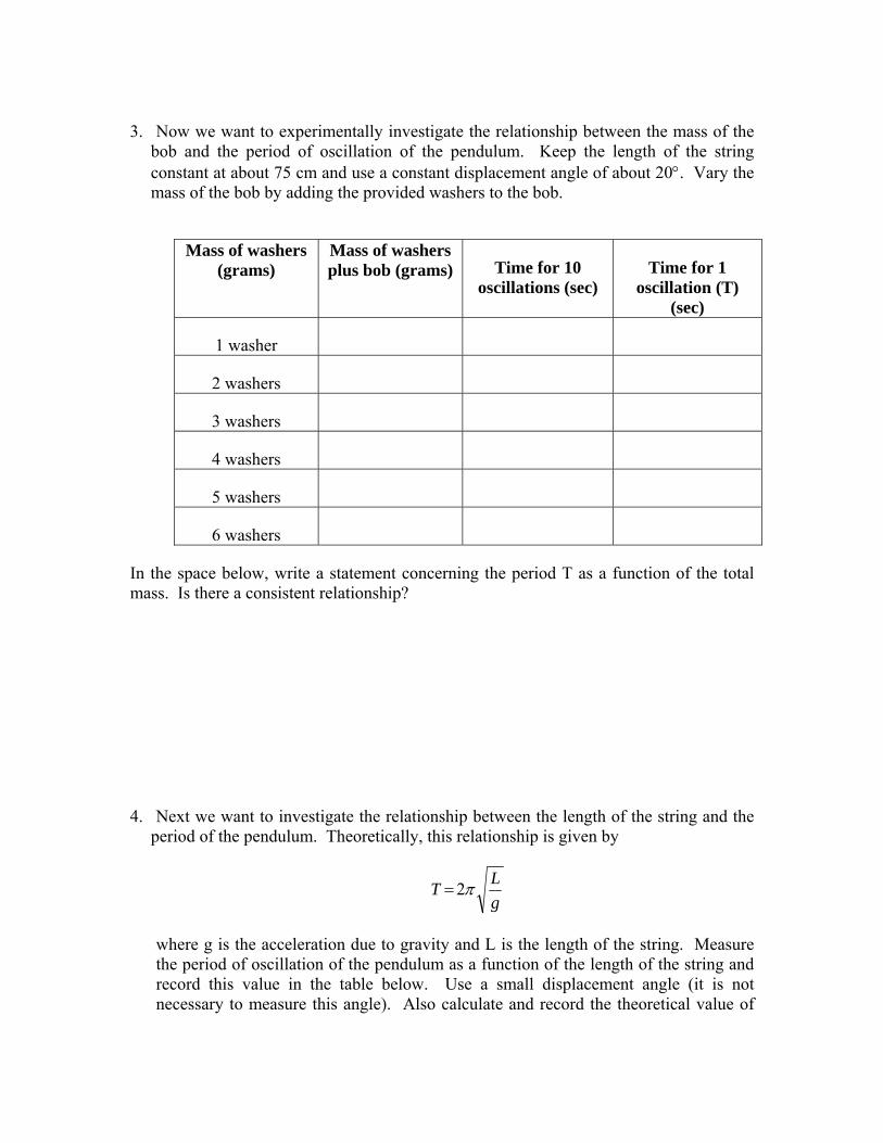
3. Now we want to experimentally investigate the relationship between the mass of the bob and the period of oscillation of the pendulum. Keep the length of the string constant at about 75 cm and use a constant displacement angle of about 20°. Vary the mass of the bob by adding the provided washers to the bob.

Mass of washers

(grams) Mass of washers plus bob (grams) Time for 10

oscillations (sec) Time for 1

oscillation (T) (sec)

1 washer

2 washers

3 washers

4 washers

5 washers

6 washers

In the space below, write a statement concerning the period T as a function of the total mass. Is there a consistent relationship?

4. Next we want to investigate the relationship between the length of the string and the period of the pendulum. Theoretically, this relationship is given by

gLT π2=

where g is the acceleration due to gravity and L is the length of the string. Measure the period of oscillation of the pendulum as a function of the length of the string and record this value in the table below. Use a small displacement angle (it is not necessary to measure this angle). Also calculate and record the theoretical value of

the period, and the percent error between the experimental value and the theoretical value using

100% ×−

=Exp

TheoryExperror .

Length (L) Time for 10 osc. (sec)

Time for 1 osc. T (sec)

T2 (sec2) Ttheory (sec) Percent error

0.20 m

0.40 m

0.60 m

0.80 m

1.00 m

1.20 m

In the space below, write a statement concerning the period T you experimentally determined and the length L of the pendulum. Is there a consistent relationship?

5. Finally, to test the equation in part 4, plot a graph of L vs the experimental value of T2. Let L be the y-axis and T2 be the x-axis. Draw a straight line best fit of the data and determine the slope m of this line using

21

22

12

12

12

TTLL

xxyy

m−−

=−−

= .

Rearranging the equation for the pendulum gives

224

TgLπ

= .

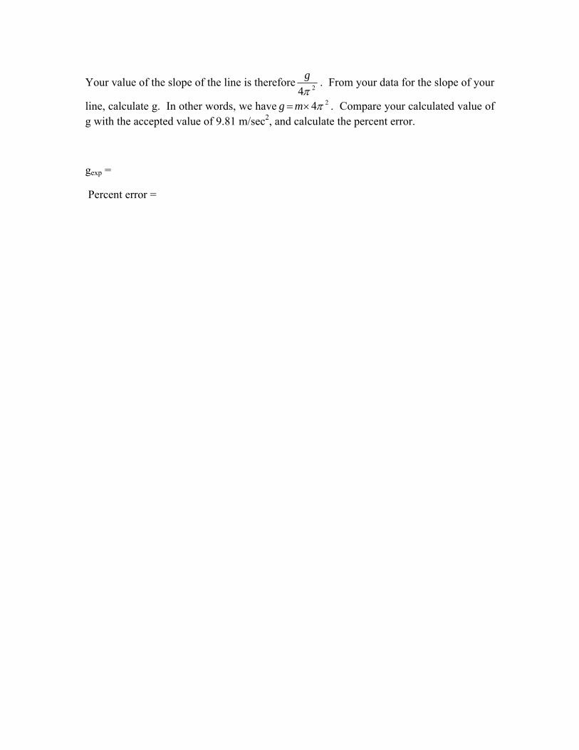
Your value of the slope of the line is therefore 24πg . From your data for the slope of your

line, calculate g. In other words, we have 24π×= mg . Compare your calculated value of g with the accepted value of 9.81 m/sec2, and calculate the percent error.

gexp =

Percent error =

Lab 6 Conservation of Momentum and Energy

The principle of conservation of momentum follows directly from Newton's laws of motion. According to this principle, if there are no external forces acting on a system containing several bodies, then the momentum of the system remains constant. In this experiment the principle is applied to the case of a collision, using a ballistic pendulum. A ball is fired by a gun into the bob of a pendulum. The initial velocity of the ball is determined in terms of the masses of the ball and pendulum bob and the height which the bob rises after impact. Theory: The momentum of a body is defined as the product of the mass of the body and its velocity. Newton's second law of motion states that the net force acting on a body is proportional to the time rate of change of momentum. Hence, if the sum of the external forces acting on a body is zero, the linear momentum of the body is constant. This is essentially a statement of the principle of conservation of momentum. Applied to a system of bodies, the principle states that if no external forces act on a system containing two or more bodies then the momentum of the system does not change. In a collision between two bodies, each one exerts a force on the other. These forces are equal and opposite, and if no other forces are brought into play, the total momentum of the two bodies is not changed by the impact. Hence the total momentum of the system after the collision is equal to the total momentum before impact. During the collision the bodies become deformed and a certain amount of energy is used to change their shape. If the bodies are not perfectly elastic, they will remain permanently distorted, and the energy used up in producing the distortion is not recovered. Inelastic impact can be illustrated by a device called a "ballistic pendulum", which is sometimes used to determine the speed of a bullet. If a bullet is fired into a pendulum bob and remains imbedded in it, the momentum of the bob and bullet just after the collision is equal to the momentum of the bullet just before the collision. This follows from the law of conservation of momentum. The velocity of the pendulum before collision is zero, while after the collision, the pendulum and the bullet move with the same velocity. Hence the momentum equation gives:

mv = M + m( )V

where m is the mass of the bullet, v is the velocity of the bullet just before impact, M is the mass of the pendulum bob, and V is the common velocity of the pendulum bob and bullet just after the collision. As a result of the collision, the pendulum with the imbedded bullet swings about its point of support, and the center of gravity of the system rises through a vertical distance h. from a measurement of this distance it is possible to calculate the velocity V. The kinetic energy of the system just after the collision must be equal to the increase in potential energy of the system as the pendulum reaches its highest point. this follows from the law of conservation of energy; here we assume that the loss of energy due to friction is negligible. The energy equation gives

(½) M + m( )V2 = (M + m )gh

where h is the vertical distance through which the center of gravity of the system rises. The left hand side of the equation represents the kinetic energy of the system just after the collision and the right hand side represents the change in potential energy of the system. Solving the above equation for V one obtains:

V = 2gh .

By substituting this value of V and the values of the masses M and m in the momentum equation, it is possible to calculate the velocity of the bullet before the collision. Thus,

v =

M + mm

2gh .

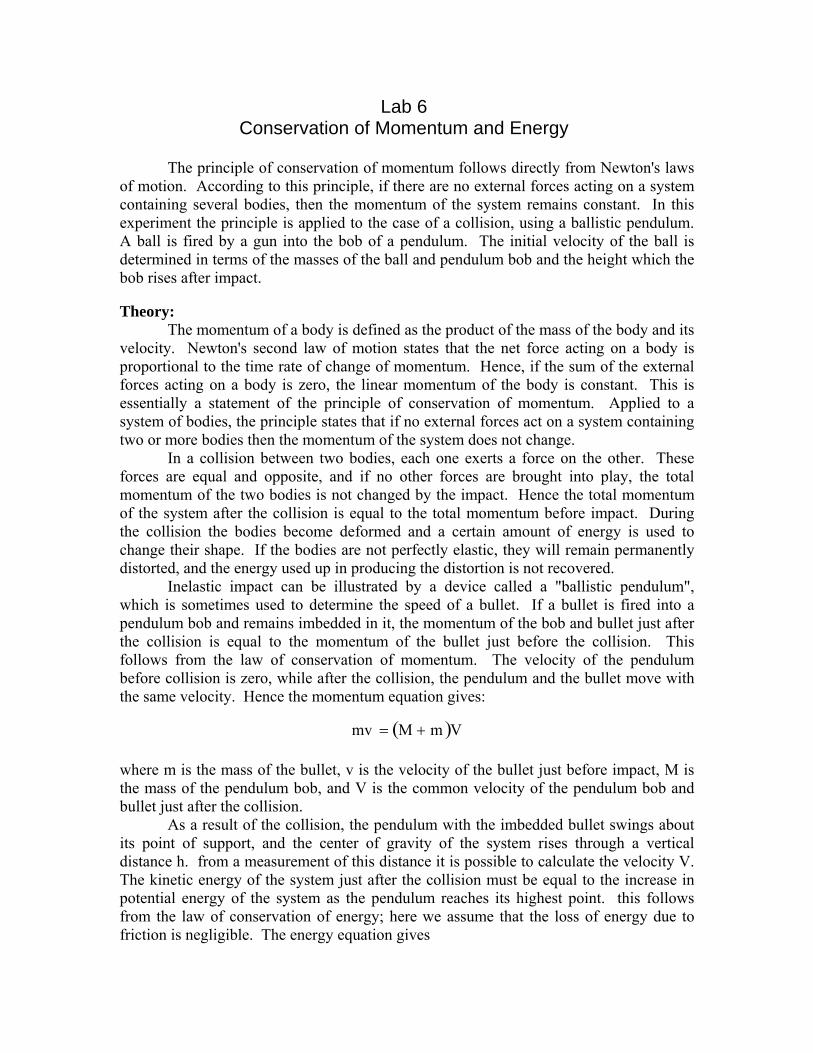
Procedure: Get the gun ready for firing. Release the pendulum from the rack and allow it to hang freely. When the pendulum is at rest, pull the trigger, thereby firing the ball into the pendulum bob. This will cause the pendulum with the ball inside it to swing up along the rack where it will be caught at its highest point. Measure the change in height of the center of mass of the pendulum bob. Repeat this procedure five times and record all five values of h and the average h av .

h 1 = h 2 = h 3 = h 4 = h 5 = h av =

Remove the pendulum bob from the apparatus and find its mass. Find the mass of the ball. Record these values: M = m = Using h av in meters, M and m in kilograms, and g in meters per second, calculate the speed of the ball. v = Using your calculated values for v and V to find the amount of energy expended in embedding the ball in the pendulum bob. ∆E =

Lab 7 Simple Harmonic Motion

Theory: Simple harmonic motion is one of the most common types of motion found in nature, and its study is therefore very important. Examples of this type of motion are found in all kinds of vibrating systems, such as water waves, sound waves, the rolling of ships, the vibrations produced by musical instruments and many others. The archetype for simple harmonic motion is a mass on the end of a spring. One of the criteria for determining whether a system will produce simple harmonic motion is that the force exerted by the system on a mass is proportional to the displacement of the mass from its equilibrium position and that the force points back toward the equilibrium position. For a spring, this force is: xkF Δ−= which obviously satisfies this requirement. This force then gives the following relationship between the acceleration and the position of the mass:

xmka Δ⎟

⎠⎞

⎜⎝⎛−= .

Using calculus, this equation can be shown to require that "period of oscillation", T (which is the time required for the mass to go through one cycle and return to its original position) is given by:

T = 2π

mk

where m is the mass of the object and k is the spring constant of the spring. Note that the period is independent of the size of the oscillation. This is true as long as the oscillation is not so big that it starts to permanently deform the spring and the force is no longer described by xkF Δ−= . We will test this result by measuring the spring constant of a spring, the mass of an object oscillating on the end of the spring, and the period of the mass' oscillation. The measured period should be equal to the value calculated using the above formula and the measured values of m and k.

Procedure: We will first measure the spring constant, k, by hanging a mass from the end of the spring and allowing the mass to come to equilibrium. At equilibrium, the force of gravity pulling down on the mass will be canceled by the force of the spring pulling up on the mass. Therefore, xkmg Δ= so

x

mgkΔ

= .

Since Δx is equal to the displacement from the equilibrium position of the spring when it has no mass attached to it, we need to first find the equilibrium position of the spring. Hang the spring from a support pole, and hang the mass hanger from its lower end. Measure the height of the bottom of the mass hanger from the table. Record this position as the equilibrium position, h0. h0 = Now, add five different masses to the hanger and record the added mass m and the height of the bottom of the mass hanger from the table h. Calculate the displacement or stretch of the spring Δx = h0 − h and record this for each mass.

m (kg) weight (N) h (m) Δx = h0 − h (m)

The spring constant k is the slope of the line found by plotting the weight of the mass as a function of Δx. Find k by plotting the weight of the mass along the y-axis and Δx along the x-axis. Draw a best fit line through these data points and then find the slope of the line. Record k and the units associated with it.

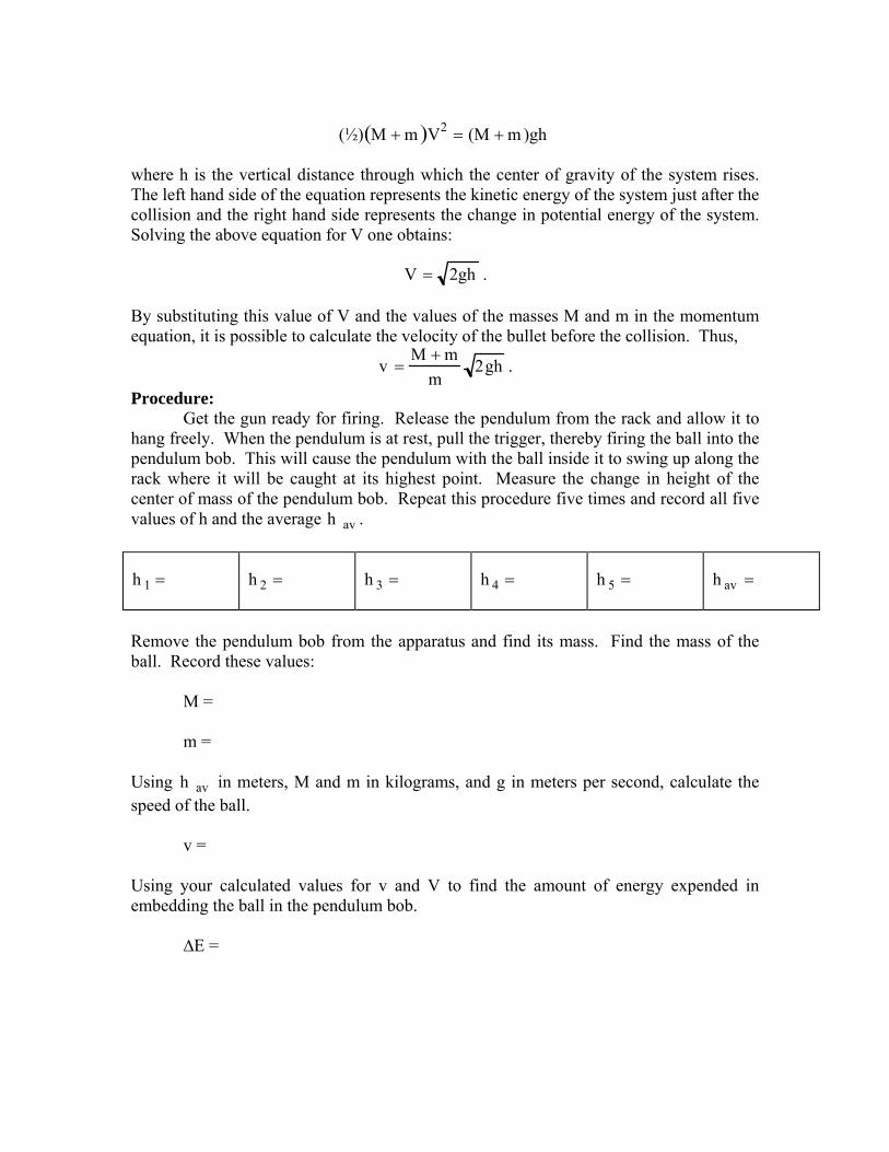
k = We will now investigate the relationship between the period of oscillation of the spring and the mass of an object attached to the spring. To do this, hang a known mass m (hanger plus added masses) on the end of the spring. The total mass that must be oscillated by the spring is this mass plus the mass of the spring ms. Measure the time (t) required for 10 oscillations. Repeat this procedure three times for different added masses, and record your results in the data table below. ms =

m t smmM += 10exp tT = kMT π= 2

Using the data you have gathered, do the calculations required to fill out the rest of the data table. For each trial, calculate the percent discrepancy between 10exp tT = and

kMT π= 2 . Record these values below.

Texp T % Difference

Lab 8 Resonance in Closed Tubes

The velocity with which a sound wave travels in a substance may be determined if the frequency of the vibration and the length of the wave are known. In this experiment the velocity of sound in air will be found by using a tuning fork of known frequency to produce a wavelength in air which can be measured by means of a resonating air column. Theory: If a vibrating tuning fork is held over a tube, open at the top and closed at the bottom, it will send air disturbances, made up of compressions and rarefactions, down the tube. These disturbances will be reflected at the closed end of the tube. If the length of the tube is such that the returning disturbances are in phase with those being sent out by the tuning fork, then resonance takes place. This means that the disturbances reinforce each other and produce a louder sound. Thus, when a tuning fork is held over a tube closed at one end, resonance will occur if standing waves are set up in the air column with a node at the closed end and a loop (or anti-node) near the open end of the tube. This can take place if the length of the tube is very nearly an odd number of quarter wave lengths of the sound waves produced by the

fork. Hence resonance will occur when L =

λ4

,3λ4

,5λ4

, etc., where L is the length of

the tube and λ is the wave length of the sound waves in air. N.B.: The center of the loop is not exactly at the open end of the tube, but is outside of it by a small distance which depends on the wave length and on the diameter of the tube. However, the distance between successive points at which resonance occurs, when the length of the tube is changed, gives the exact value of a half wave length. The relation between the velocity of sound, the frequency, and the wave length is given by the equation: v = fλ.

The velocity can be calculated from the above equation if the wave length and the frequency are both known. The velocity of sound in air depends on the temperature of the air by:

v =

γRTM

.

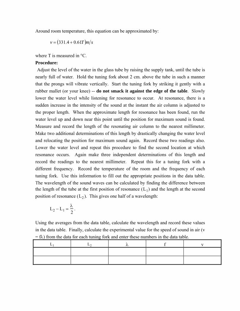
Around room temperature, this equation can be approximated by: ( ) smTv 61.04.331 += where T is measured in °C. Procedure: Adjust the level of the water in the glass tube by raising the supply tank, until the tube is nearly full of water. Hold the tuning fork about 2 cm. above the tube in such a manner that the prongs will vibrate vertically. Start the tuning fork by striking it gently with a rubber mallet (or your knee) -- do not smack it against the edge of the table. Slowly lower the water level while listening for resonance to occur. At resonance, there is a sudden increase in the intensity of the sound at the instant the air column is adjusted to the proper length. When the approximate length for resonance has been found, run the water level up and down near this point until the position for maximum sound is found. Measure and record the length of the resonating air column to the nearest millimeter. Make two additional determinations of this length by drastically changing the water level and relocating the position for maximum sound again. Record these two readings also. Lower the water level and repeat this procedure to find the second location at which resonance occurs. Again make three independent determinations of this length and record the readings to the nearest millimeter. Repeat this for a tuning fork with a different frequency. Record the temperature of the room and the frequency of each tuning fork. Use this information to fill out the appropriate positions in the data table. The wavelength of the sound waves can be calculated by finding the difference between the length of the tube at the first position of resonance ( L1) and the length at the second position of resonance ( L2 ). This gives one half of a wavelength:

L2 − L1 =

λ2

.

Using the averages from the data table, calculate the wavelength and record these values in the data table. Finally, calculate the experimental value for the speed of sound in air (v = fλ) from the data for each tuning fork and enter these numbers in the data table.

L1 L2 λ f v

Using the measured room temperature, calculate the theoretical value of the speed of sound in air from the equation: v = 331.4 + 0.6T( ) m s . Record this value and compare it with the average of the two experimentally determined values. What is the percent discrepancy? Now, repeat the experiment with carbon dioxide in the tube rather than air. The theoretical value of the speed of sound in carbon dioxide is ( ) smT48.03.262v +=

Use the preceeding formula for the speed of sound and your tuning fork’s frequency to predict where the second resonance point should be (approximately). Lower the water level in the tube about ten centimeters below where the second resonance point should be. You will be provided with two tablets of Alka-Seltzer. Take one tablet and drop it into the tube. The tablet to should immediately begin to fizz and dissolve in the water, filling up the tube with carbon dioxide and pushing out the air. Allow this to continue until the tablet is nearly gone. If you are not going to immediately begin performing measurements, use the rubber plug provided to seal the tube and keep the carbon dioxide atmosphere pure. Perform your measurements as before, but by raising the water level only; you cannot lower the water level at any point as this will draw air into the tube and contaminate the results. You essentially will have only one try at finding the second and first resonance point, so be careful not to overshoot. Repeat for your second tuning fork (you will use the second tablet to fill the tube with CO2 again). Calculate the experimental value for the speed of sound in carbon dioxide (v = fλ) from the data for each tuning fork and enter these numbers in the data table.

L1 L2 λ f v

Record this value and compare it with the average of the two experimentally determined values in carbon dioxide. What is the percent discrepancy?

Lab 9 Archimedes' Principle

Buoyancy is the name given to the ability of a fluid to sustain a body floating in it, or to diminish the apparent weight of a body immersed in it. The size of the buoyant force was discovered by Archimedes to be exactly equal to the weight of the fluid displaced by the object. In this experiment, we will use Archimedes' Principle to determine the specific gravity (and also the density) of a solid which is heavier than water and a solid which is lighter than water. Theory:

Archimedes' Principle states that the apparent loss of weight of a body immersed in a fluid is equal to the weight of the fluid displaced. This means that the difference in weight of an object when it is weighed in air and then weighed while submerged in a liquid is equal to the weight of the amount of liquid which would occupy the same volume as the object. Let's specialize to water as our liquid since we know that water has

a density of 312 cmg

OH =ρ . If the weight in air of an object which has a volume V is Wair,

and the weight submerged in water is Wsub, then the difference in weights will give the weight of an equivalent volume of water:

OHsubair WWW 2=− .

The specific gravity of an object is the ratio of its density to the density of a fluid in which it will be submerged (water, in our case). If an objects specific gravity is greater than 1, it will sink in that fluid; if its specific gravity is less than 1, it will float. The specific gravity of the object can be found as follows: if ρ is the density of the object and

OH 2ρ is the density of our liquid, then it follows that

VW

VW OH

OHair 2

2 , == ρρ

and

OH

air

OH

air

OH WW

VWVWS

222

===ρ

ρ

subair

air

WWWS−

=→

To find the density of the object, one needs merely to multiple the specific gravity by the

density of the liquid used. Since we are using water with a density of 312 cmg

OH =ρ , this

merely adds the units of density to the unitless number of specific gravity. Finally, to find the specific gravity of an object which floats in water, we cannot simply weigh it in water (since it will not completely submerge). We have to tie a sinker to the object to keep it submerged. When we weight the object, we then find the combined weight of the object and of the sinker. If we have already determined the weight of the sinker when submerged, we merely need to subtract that from the combined weight to find the weight of the submerged object alone. Note, this weight ends up being a negative number, which indicates that the object, when submerged, floats up towards the surface rather than sinks down. When one wants to find the density of objects with regular simple shapes, it is easier to just weight them and then measure their dimensions to calculate their volumes directly. An object’s density is then ρ = M/V by definition. Archimedes’ Principle is most useful for finding the density of objects with irregular shapes, like the sinker. Indeed, this is what the Principle was originally invented to do (measure the density of a king’s crown to determine if it was truly made of pure gold or if the craftsman cheated by adding cheaper metals to the alloy). You will double check your wood density by also finding it directly. Procedure:

1. Weigh the copper sinker in air. 2. Weigh the copper sinker in water. 3. Weigh the wooden block in air. 4. Weigh the wooden block with the sinker, both submerged. 5. Measure the three side lengths of the wooden block with Vernier calipers. side 1: side 2: side 3: 6. Look up the density of copper in a textbook or on the internet.

Calculate the density of the wood directly from its mass and volume:

Calculate the specific gravity (density) of the wood using Archimedes’ Principle: Calculate the specific gravity (density) of the copper using Archimede’s Principle: Calculate the percent deviation between the two densities of wood you have experimentally determined. Comment. Calculate the percent error between your experimentally determined density of the copper sinker and the actual density of copper you have looked up. Comment.