Embed Size (px)
Citation preview
CHAPTER 7
PIPELINE TRANSPORTATION OF OIL
7.1. Pressure waves, waterhammer
Pressure wave may occur in pipelines transporting fluids if the velocity of the flowing liquid suddenly changes. The pressure wave propagates by the sonic velocity from the point ofa leak or a device, initiating the change of pressurc in both, or perhaps even more connecting pipeline branches. During propagation the wave’s amplitude is reduced, damped. and perhaps i t is even reflected. The pressure wave may be of positive character when a sudden decrease in the velocity of the flowing fluid may cause a rise in the pressure: and i t may be also of negative character when the sudden rise in velocity of the fluid may result in dropping of pressure.
7.1.1. The reasons of the waterhammer phenomenon and its mathematical representation
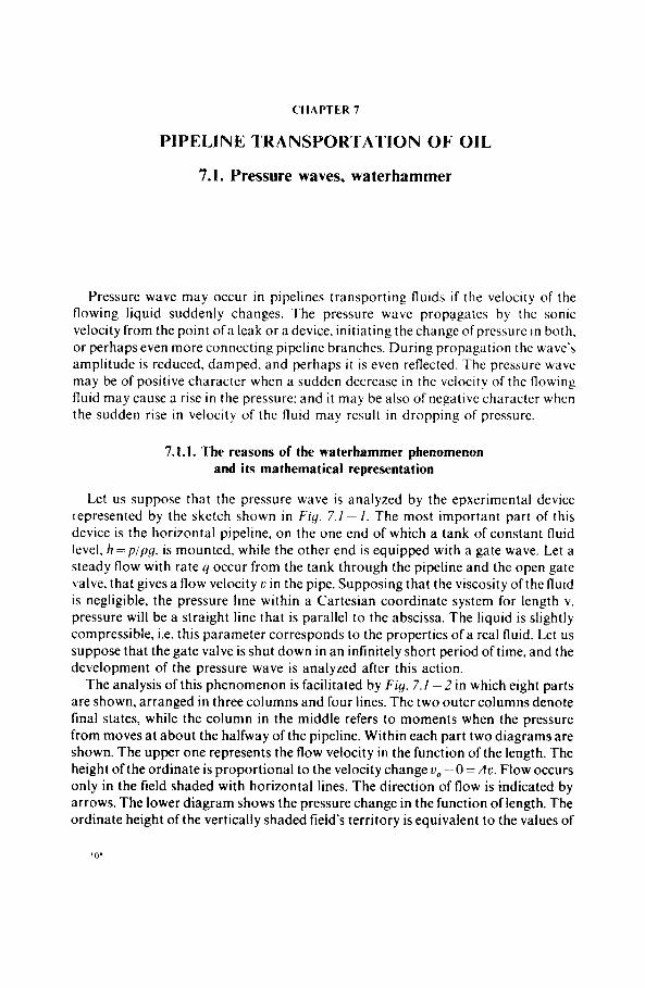
Let us suppose that the pressure wave is analyzed by the epxerimental device represented by the sketch shown in Fiq. 7.1 - 1. The most important part of this device is the horizontal pipeline, on the one end of which a tank of constant fluid level, h = p / p y , is mounted, while the other end is equipped with a gate wave. Let a steady flow with rate y occur from the tank through the pipeline and the open gate valve, that gives a flow velocity u in the pipe. Supposing that the viscosity of the fluid is negligible, the pressure line within a Cartesian coordinate system for length v. pressure will be a straight line that is parallel to the abscissa. The liquid is slightly compressible, i.e. this parameter corresponds to the properties ofa real fluid. Let us suppose that the gate valve is shut down in an infinitely short period of time, and the development of the pressure wave is analyzed after this action.
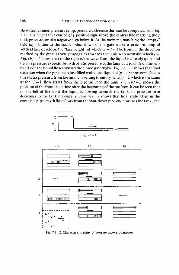
The analysis of this phenomenon is facilitated by Fig. 7.1 - 2 in which eight parts are shown, arranged in three columns and four lines. The two outer columns denote final states, while the column in the middle refers to moments when the pressure from moves at about the halfway of the pipeline. Within each part two diagrams are shown. The upper one represents the flow velocity in the function of the length. The height of the ordinate is proportional to the velocity change v, - 0 = Ac. Flow occurs only in the field shaded with horizontal lines. The direction of flow is indicated by arrows. The lower diagram shows the pressure change in the function of length. The ordinate height of the vertically shaded field’s territory is equivalent to the values of
148 7 PIPELINE TRANSPORTATION OF OIL
dp waterhammer, pressure jump, pressure difference that can be computed from Eq. 7.1 - 1, a height that can be of a positive sign above the central line marking the p tank pressure, or of a negative sign below it. At the moment, matching the “empty” field (a)- 1, due to the sudden shut down of the gate walve a pressure jump of vertical face develops, the “face height” of which is + dp. The front, in the direction marked by the great arrow, propagates towards the tank with acoustic velocity w. Fig. (6) - 1 shows that to the right of the wave front the liquid is already quiet and here its pressure exceeds the hydrostatic pressure of the tank by A p , while on the left- hand side the liquid flows toward the closed gate walve. Fig. ( c ) - 1 shows that final situation when the pipeline is just filled with quiet liquid of(p + dp) pressure. Due to this excess pressure, from the moment suiting to empty field (c) - 2, which is the same as for ( c ) - 1, flow starts from the pipeline into the tank. Fig. ( b ) -2 shows the position of the front in a t time after the beginning of the outflow. It can be seen that on the left of the front the liquid is flowing towards the tank, its pressure here decreases to the tank pressure. Figure ( a ) -2 shows that final state when in the complete pipe length fluid flows from the shut-down pipe end towards the tank, and
Fig. 7.1 - I
-- - I - - 3
7. I. PRESSURE WAVES. W A T E R H A M M E R 149
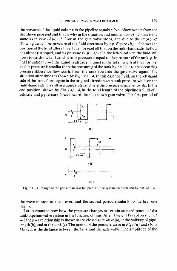
the pressure of the liquid column in the pipeline equals p. No inflow occurs from the shutdown pipe end and that is why in the situation and moment of(u) - 2, that is the same as in case of (u)-3, flow at the gate valve stops, and due to the impact of “flowing away” the pressure of the fluid decreases by A p . Figure ( h ) - 3 shows the position ofthe front after t time. I t can be read off that on the right-hand side the flow has already stopped, and its pressure is (p- LIP). On the left-hand side the fluid still flows towards the tank. and here its pressure is equal to the pressure of the tank, p. In final situation (c)- 3 the liquid is already in quiet in the total length of the pipeline, and its pressure is smaller than the pressure p of the tank by Ap. Due to the occurring pressure difference flow starts from the tank towards the gate valve again. The situation after time t is shown by Fig. (h) - 4 . In this case the fluid, on the left-hand side ofthe front, flows again in the original direction with tank pressure, while on the right-hand side it is still in a quiet state, and here the pressure is smaller by Ap. In the end position, shown by F i g . ( a ) - 4 , in the total length of the pipeline a fluid of 1‘
velocity and p pressure flows toward the shut-down gate valve. The first period of
0 pw 4 L/w
i b )
0 ’+
( C )
Fig. 7.1 -3. Change of the pressure in selected points of the system charactenzed by Fig. 7.1 - I
the wave motion is, then, over, and the second period similarly to the first one begins.
Let us examine now how the pressure changes at certain selected points of the tank-pipeline-valve system in the function of time. After Thielen (1972b) on Fig. 7.1 -3 the p- t relationship is shown at the closed gate valve (a), at the halfway of pipe- length (b), and at the tank (c). The period of the pressure wave in F i g s (a ) and ( b ) is 4Lfw. L is the distance between the tank and the gate valve. The amplitude of the
pressure wave. A p may be computed from Fq. 7.1 ~- 1, and this value will not change for 2L/w length of time at the gate valve and for l , /w at the halfway. A t the t ank (c) , the pressure is the same as the static pressure of the fluid, p = kpq.
For the calculation of the waterhammer pressure change due to sudden velocity change Allievy and Joukowsky recommended a formula dcrivcd from thc momentum equation already at the beginning of the 20th century:
A p = p . M'. A ( * 7.1 1
Pressure rise A p is directly proportional to the velocity drop Ai.; thc factor o f proportionality is the product of the density of the fluid and t h c acoustic velocity in the fluid-tilled pipeline, p . w.
For several problems being important in practice the above equation does not offer solution. These are mainly as follows: ( i ) how the pressure changes at different points ofthe liquid transporting system; ( i i ) how the pressure change is influcnccd by the devices that are responsible for thechange in the velocity ofthe fluid (e.g. valves, pumps), ( i i i ) what is the impact of the physical parameters of the real fluids; and, finally (iv) how the configuration and elasticity of the pipeline system influcncc the
1
Fig. 7.1 - -4. Forces acting on f l u d particle moving in Y direction. idler Strcctcr a i d Wylie (1967)
process. Based on the research results of the past decades these questions can be answered with proper accuracy.
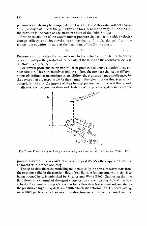
The up-to-date theories, modelling mathcrnatically the pressure waves start from the relations valid for the transient flow of real fluids. A fundamental work, that is to be mentioned here, is published by Streeter and Wylie (1967). Supposing (hat the fluid flows in a channel of divergent cross-section shown on Fig. 7.1 - 4 , the flow velocity in a cross-section perpendicular to the flow direction is constant, and due to the pressure change the system is submitted to elastic deformation. The forces acting on a fluid particle which moves in x direction in a divergent channel are the
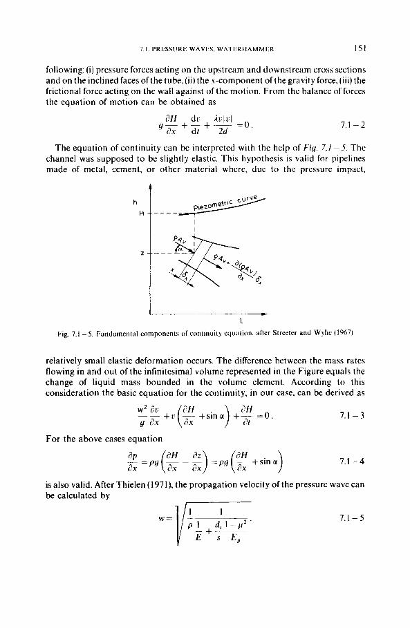
7 I PRLS31IRL WAVLS. W A T l R l l A M M l R 151
following: ( i ) pressure forces acting on the upstream and downstream cross sections and on the inclined faces ofthe tube, ( i i ) the Ic-component of the gravity force, ( i i i ) the frictional force acting on the wall against of the motion. From the balance of forces the equation of motion can be obtained as
7.1 - 2
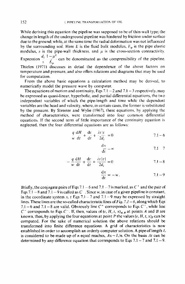
The equation of continuity can be interpreted with the help of F i g . 7.1 - 5 . The channel was supposed to be slightly elastic. This hypothesis is valid for pipelines made of metal, cement, or other material where, due to the pressure impact.
L
Fig. 7.1 - 5. Fundamental components cif continuity equation. after Strceter and Wylie (1967)
relatively small elastic deformation occurs. The difference between the mass rates flowing in and out of the infinitesimal volume represented in the Figure equals the change of liquid mass bounded in the volume element. According to this consideration the basic equation for the continuity, in our case, can be derived as
For the above cases equation
d p - ( 6 H d z )
- -py - - - =pq - +sina ax a x c?x (z . )
7.1 - 3
7.1 - 4
is also valid. After Thielen (1971). the propagation velocity of the pressure wave can be calculated by
7.1 - 5
152 7. PIPELINE TRAXSPORTATION OF O I L
While deriving this equation the pipeline was supposed to be of thin-wall type; the change in length of the underground pipeline was hindered by friction under surface due to the ground; while, at the same time the radial deformation was not influenced by the surrounding soil. Here E is the fluid bulk modulus, E , is the pipe elastic modulus, s is the pipe-wall thickness, and ,u is the cross-section contractivity.
Expression 2 __ can be denominated as the compressibility of the pipeline.
Thielen (1971) discusses in detail the dependence of the above factors on temperature and pressure, and also offers relations and diagrams that may be used for computation.
From the above basic equations a calculation method may be derived, to numerically model the pressure wave by computer.
The equations of motion and continuity, Eqs 7.1 - 2 and 7.1 - 3 respectively. may be expressed as quasi-linear, hyperbolic, and partial differential equations, the two independent variables of which the pipe-length and time while the dependent variables are the head and velocity, where, in certain cases, the former is substituted by the pressure. By Streeter and Wylie (1967). these equations, by applying the method of characteristics, were transformed into four common differential equations. If the second term of little importance of the continuity equation is neglected. then the four differential equations are as follows:
d I - /? s E ,
q dH dc i c l c l -~ - + - + -- = o w’ dt dt 2d,
d Y
dt - =M’
- d x
dt - - - w .
7.1 -6
7.1 -7
7.1 -8
7.1 -9
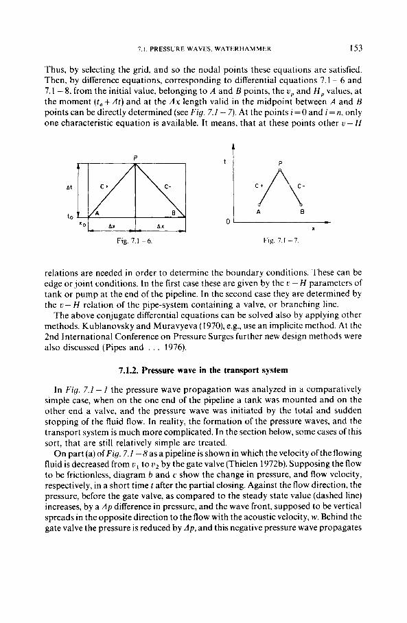
Briefly, the conjugate pairs of Eqs 7.1 - 6 and 7.1 - 7 is marked, as C’ and the pair of Eqs 7.1 - 8 and 7.1 - 9 is called as C -. Since w, in case of a given pipeline is constant, in the coordinate system ?I, t Eqs 7.1 - 7 and 7.1 -9 may be expressed by straight lines. These lines are the so-called characteristic lines of F i g . 7.1 -6, along which Eqs 7.1 - 6 and 7.1 - 8 are valid. Obviously line C + corresponds to Eqs C+, while line C- corresponds to Eqs C-. If, then, values of (u , H , t , . x ) ~ . ~ at points A and B are known, then, by applying the four equations at point P the values ( u , H , t , x ) ~ can be computed. For the sake of numerical solution the above relations should be transformed into finite difference equations. A grid of characteristics is now established in order to accomplish an orderly computer solution. A pipeaf length L is considered to be made up of n equal reaches, A x = L/n. On the basis A t can be determined by any difference equation that corresponds to Eqs 7.1 - 7 and 7.1 -9.
1. I . PRESSURE WAVES. W A T E R H A M M E R 153
Thus, by selecting the grid, and so the nodal points these equations are satisfied. Then, by difference equations, corresponding to differential equations 7.1 - 6 and 7.1 - 8, from the initial value, belonging to A and B points, the u p and H , values, at the moment ( t , + A t ) and at the A x length valid in the midpoint between A and B points can be directly determined (see Fig. 7.1 - 7) . At the points i=O and i = n, only one characteristic equation is available. It means, that at these points other u - H
P
Aa A x -
t
0- X
Fig. 7. I - 6 . Fig. 7.1 - 7
relations are needed in order to determine the boundary conditions. These can be edge or joint conditions. In the first case these are given by the c- H parameters of tank or pump at the end of the pipeline. In the second case they are determined by the u - H relation of the pipe-system containing a valve, or branching line.
The above conjugate differential equations can be solved also by applying other methods. Kublanovsky and Muravyeva (1970), e.g., use an implicite method. At the 2nd International Conference on Pressure Surges further new design methods were also discussed (Pipes and . . . 1976).
7.1.2. Pressure wave in the transport system
In Fig . 7.1 - I the pressure wave propagation was analyzed in a comparatively simple case, when on the one end of the pipeline a tank was mounted and on the other end a valve, and the pressure wave was initiated by the total and sudden stopping of the fluid flow. In reality, the formation of the pressure waves, and the transport system is much more complicated. In the section below, some cases of this sort, that are still relatively simple are treated.
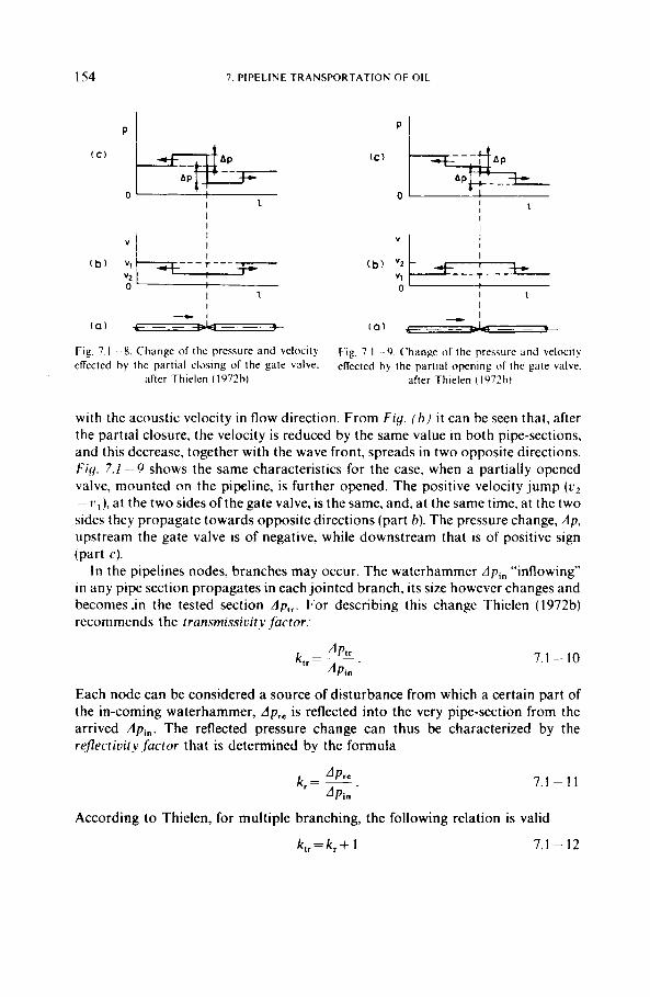
On part (a) of Fig. 7.1 -8 as a pipeline is shown in which the velocity of the flowing fluid is decreased from u , to u2 by the gate valve (Thielen 1972b). Supposing the flow to be frictionless, diagram b and c show the change in pressure, and flow velocity, respectively, in a short time t after the partial closing. Against the flow direction, the pressure, before the gate valve, as compared to the steady state value (dashed line) increases, by a A p difference in pressure, and the wave front, supposed to be vertical spreads in the opposite direction to the flow with the acoustic velocity, w. Behind the gate valve the pressure is reduced by A p , and this negative pressure wave propagates
I54 7. PIPELINE TRANSPORTATION OF 0 1 1
( c ' 0 k3!57 I I 1
I I
V l I
r---- ( b ) "2 "e 0
I I I
- 1 - _ - -. (a)
Fig. 7. I - 8. Change of the pressure and velocity effected hy the partial closlng of the gate valve.
after Thielen (197%)
01 I I
I I I
I I I
I I 0'
I - + I
( 0 ) + .- - _ -
Fig. 7.1 -9. Change of the pressure and velocity elTected by the partial opening of the gate valve.
after Thielen (1972bj
with the acoustic velocity in flow direction. From Fig. ( h ) it can be seen that, after the partial closure, the velocity is reduced by the same value in both pipe-sections, and this decrease, together with the wave front, spreads in two opposite directions. F i g . 7.1 --9 shows the same characteristics for the case, when a partially opened valve, mounted on the pipeline, is further opened. The positive velocity jump ( u 2 - v l ) , at the two sides of the gate valve, is the same, and, at the same time, at the two sides they propagate towards opposite directions (part h). The pressure change, A p , upstream the gate valve is of negative, while downstream that is of positive sign (part c) .
In the pipelines nodes, branches may occur. The waterhammer Apin "inflowing" in any pipe section propagates in each jointed branch, its size however changes and becomes .in the tested section Aprr. For describing this change Thielen (1972b) recommends the transmissivit): factor:
7.1 - 10
Each node can be considered a source of disturbance from which a certain part of the in-coming waterhammer, Ap,, is reflected into the very pipe-section from the arrived Apin. The reflected pressure change can thus be characterized by the reflectivity factor that is determined by the formula
7.1-11
According to Thielen, for multiple branching, the following relation is valid
k l , = k r + 1 7.1 - 12
7 I PRESSURI: W A V f S . W A T I . K H A M M 1 R I55
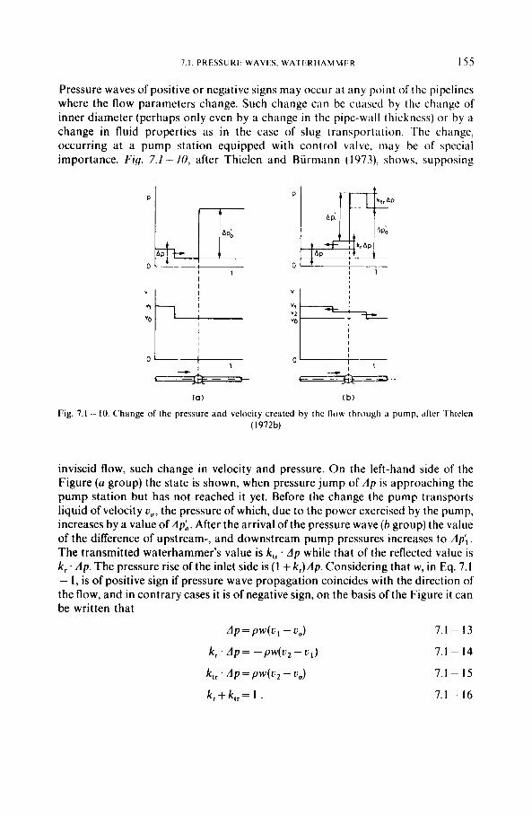
Pressure waves of positive or negative signs may occur a t any point of the pipelines where the flow parameters change. Such change can be cuascd by the change of inner diameter (perhaps only even by a change in thc pipe-wall thickness) or by a change in fluid properties as in the case of slug transportation. The change, occurring at a pump station equipped with control valvc, may be o f special importance. Fig. 7.1 - 10, after Thielen and Biirmann (1973). shows, supposing
I I I I
I I I I
- 1 - A _ _ _ _ 0-
_ _ _ - - (a) ( b )
Fig. 7.1 - 10. Change of the pressure and velocity created by the flow through a pump, after Thielen (1972b)
inviscid flow, such change in velocity and pressure. On the left-hand side of the Figure (a group) the state is shown, when pressure jump of A p is approaching the pump station but has not reached it yet. Before the change the pump transports liquid of velocity u,, the pressure of which, due to the power exercised by the pump, increases by a value of Apb. After the arrival of the pressure wave (b group) the value of the difference of upstream-, and downstream pump pressures increases to Ap’, . The transmitted waterhammer’s value is k,, . dp while that of the reflected value is k , . dp. The pressure rise of the inlet side is ( I + k , ) A p . Considering that w, in Eq. 7.1 - 1, is of positive sign if pressure wave propagation coincides with the direction of the flow, and in contrary cases i t is of negative sign, on the basis of the Figure i t can be written that
A P = P W ( 0 , - 00) 7.1 ~ 13
7.1 ~ 14 k , . A p = -pw(u, - u l )
7.1 - I5
7.1 - 16
156 7. PIPELINE TRANSPORTATION OF OIL
It should be noted that the sign of k, is of opposite character, as compared with the case valid for branching. From these relations it can be derived that the increased pressure difference is
A ~ ; = A P ~ - ~ A P + ~ ~ W ( U , - U , ) . 7.1 - 17
This relation, together with Eqs 7.1 - 14 and 7.1 - 15 provide the possibility, in case characterized by Fig. 7.1 - 10, for computing the transmissivity and reflectivity factors on the basis ofthe values measured in the course of the pressure change. With proper alteration of the signs this computation method is also valid for negative pressure waves.
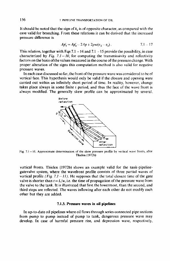
In each case discussed so far, the front of the pressure wave was considered to be of vertical face. This hypothesis would only be valid if the closure and opening were carried out within an infinitely short period of time. In reality, however, change takes place always in some finite t period, and thus the face of the wave front is always modified. The generally skew profile can be approximated by several,
Before reflection
Fig. 7.1 - 1 I . Approximate determination of the skew pressure profile by vertical wave fronts, after Thielen (1972b)
vertical fronts. Thielen (1972b) shows an example valid for the tank-pipeline- gatevalve system, where the wavefront profile consists of three partial waves of vertical profile (Fig. 7.1 - 1 1) . He supposes that the total closure time of the gate valve is shorter than t = L/w, i.e. the time of propagation of the pressure wave from the valve to the tank. It is illustrated that first the lowermost, than the second, and third steps are reflected. The waves inflowing after each other do not modify each other but they are added.
7.1.3. Pressure waves in oil pipelines
In up-to-date oil pipelines where oil flows through series connected pipe sections from pump to pump instead of pump to tank, dangerous pressure wave may develop. In case of harmful pressure rise, and depression wave, respectively,
1 I PRESSIJRE WAVES. W A T E R H A M M E R 157
cavitation damaging the pump may occur. The speed of pressure increase of the stopped fluid flow may achieve the value of 10 bar/s; the pressure rise may be as great as 30 bars, and may propagate in the pipeline at a velocity of I km/s (Vladimirsky et u1. 1976). The rate of pressure change may differ from the value that can be computed from relations valid for inviscid fluids. Another difference is that in the course of the propagation the size of the pressure change may be modified. Explanation for this phenomenon is given by Streeter and Wylie (1967). Its essence is as follows.
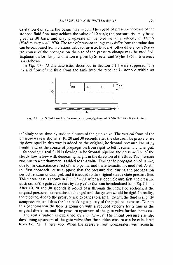
In Fig. 7 .1 - I 2 characteristics described in Section 7.1 . I were supposed. The inviscid flow of the fluid from the tank into the pipeline is stopped within an
‘ I _ _ _ _ _ _ +
I-ig. 7.1 ~ 12. Sirnulalion I of pressure wave propagation. dfter Streeter and Wylie (1967)
infinitely short time by sudden closure of the gate valve. The vertical front of the pressure wave is shown at 10,20 and 30 seconds after the closure. The pressure rise dp developed in this way is added to the original, horizontal pressure line of po height, and in the course of propagation from right to left it remains unchanged.
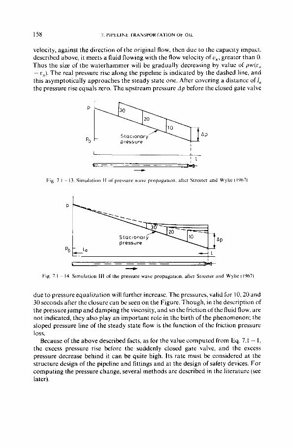
Supposing a real fluid is flowing in horizontal pipeline the pressure line of the steady flow is kew with decreasing height in the direction of the flow. The pressure rise, due to waterhammer, is added to this value. During the propagation of its size, due to the capacitance effect of the pipeline, and the attenuation is modified. As for the first approach, let us suppose that the pressure rise, during the propagation period, remains unchanged, and it is added to the original steady state pressure line. This unreal case is shown in Fig. 7.1 - 13. After a sudden closure, first, the pressure upstream of the gate valve rises by a A p value that can be calculated from Eq. 7.1 - 1 . After 10, 20 and 30 seconds it would pass through the indicated sections, if the original pressure line remains unchanged and the system would be rigid. In reality, the pipeline, due to the pressure rise expands to a small extent, the fluid is slightly compressible, and thus the line packing capacity of the pipeline increases. Due to this phenomenon the flow is going on with a reduced velocity for a time in the original direction, and the pressure upstream of the gate valve further increases.
The real situation is explained by Fig. 7.1 - 14. The initial pressure rise A p , developing upstream of the gate valve after the sudden closure can be calculated from Eq. 7.1 - 1 here, too. When the pressure front propagates, with acoustic
158 7. P l P t L l N E TRANSPORTATION OF 011
velocity, against the direction of the original flow, then due to the capacity impact, described above, it meets a fluid flowing with the flow velocity of u,, greater than 0. Thus the size of the waterhammer will be gradually decreasing by value of p w ~ ( c , , - ti,). The real pressure rise along the pipeline is indicated by the dashed line, and this asymptotically approaches the steady state one. After covering a distance of I, the pressure rise equals zero. The upstream pressure dp before the closed gate valve
I 1 - - - - _ _ _ - - Iig. 7.1 - 13. Simirlation I1 o f pressure wave propagation. after Streerer dnci Wyhe (1067)
- - - - - - - - - - --t
Fig. 7.1 ~ 14. Simulation Ill of the pressure wave propagation. after Srreeter and Wyhe (1967)
due to pressure equalization will further increase. The pressures, valid for 10,20 and 30 seconds after the closure can be seen on the Figure. Though, in the description of the pressure jump and damping the viscosity, and so the friction of the fluid flow, are not indicated, they also play an important role in the birth of the phenomenon; the sloped pressure line of the steady state flow is the function of the friction pressure loss.
Because of the above described facts, as for the value computed from Eq. 7.1 - I , the excess pressure rise before the suddenly closed gate valve, and the excess pressure decrease behind it can be quite high. Its rate must be considered at the structure design of the pipeline and fittings and at the design of safety devices. For computing the pressure change, several methods are described in the literature (see later).
7 I . PRESSURE WAVES. W A T E R H A M M E R 159
In the previous section, basically, the reasons in the change of velocity were thought to be the opening and closure of valves. For the change in the velocity of the flowing fluid in the oil pipeline several other factors may be responsible, among which the most important are: the starting and stopping of pumps; the change in the energy supply of the pump driving motor; the instability of the head curve of the centrifugal pump; the normal operation of the piston pumps; the sudden change in the oil level within the tank; the vibrations within the pipe-system; and the sudden breaks, arid leaks in the pipeline.
The reldtion between centrifugal pumps, and the pressure waves is of outstanding importancc. The change in the performance of the centrifugal pumps may create, on the one hand, pressure waves, and on the other hand, the pressure waves, developing at other spots, are modified by the pumps while passing through them. This passing may cause damages, and even if damages do not occur, the pressure wave is modified, and this impact must be considered in the further modelling.
I t must be noted that piston pumps may provoke pressure wave, however, the pressure waves, emerging upstream of these pumps do not pass through them. That is why a piston pump can be considered as a nodal point that divides the transporting system into inflow and outflow sections that are independent of each other.
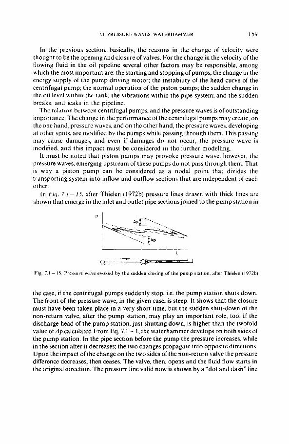
In Fig. 7.1 -IS, after Thielen (1972b) pressure lines drawn with thick lines are shown that emerge in the inlet and outlet pipe sections joined to the pump station in
1
J J _ _ _ -
Fig. 7.1 - 15. Pressure wave evoked by the sudden closing of the pump station. after Thielen (1972b)
the case, if the centrifugal pumps suddenly stop, i.e. the pump station shuts down. The front of the pressure wave, in the given case, is steep. I t shows that the closure must have been taken place in a very short time, but the sudden shut-down of the non-return valve, after the pump station, may play an important role, too. If the discharge head of the pump station, just shutting down, is higher than the twofold value of dp calculated From Eq. 7.1 - I , the waterhammer develops on both sides of the pump station. In the pipe section before the pump the pressure increases, while in the section after it decreases; the two changes propagate into opposite directions. Upon the impact of the change on the two sides of the non-return valve the pressure difference decreases, then ceases. The valve, then, opens and the fluid flow starts in the original direction. The pressure line valid now is shown by a “dot and dash” line
160 7 PIPELINE TRANSPORTATION OF OIL
in the Figure. lfthe outlet pressure of the shutting-down pump station is ofa smaller value than that of the double of the waterhammer then the non-return valve does not shut down. The throttling impact of the shut-down pump, however, must be considered even in this case.
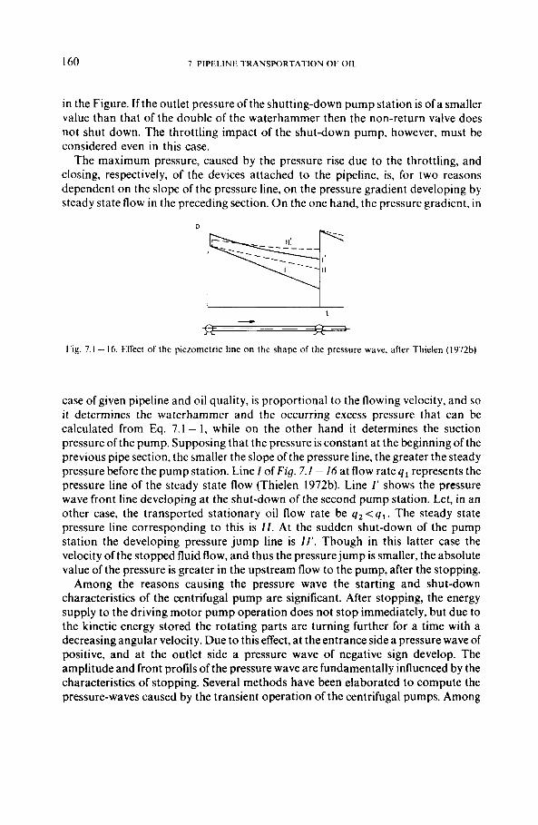
The maximum pressure, caused by the pressure rise due to the throttling, and closing, respectively, of the devices attached to the pipeline, is, for two reasons dependent on the slope of the pressure line, on the pressure gradient developing by steady state flow in the preceding section. On the one hand, the pressure gradient, in
1 - Fig. 7.1 - 16. Erect of the piezornetric line on the shape of the pressure wave, after Thielen (1972b)
case of given pipeline and oil quality, is proportional to the flowing velocity, and so it determines the waterhammer and the occurring excess pressure that can be calculated from Eq. 7.1 - 1, while on the other hand i t determines the suction pressure of the pump. Supposing that the pressure is constant at the beginning of the previous pipe section, the smaller the slope of the pressure line, the greater the steady pressure before the pump station. Line I of F i g . 7.1 - 16 at flow rate q 1 represents the pressure line of the steady state flow (Thielen 1972b). Line I' shows the pressure wave front line developing at the shut-down of the second pump station. Let, in an other case, the transported stationary oil flow rate be q2 < q l . The steady state pressure line corresponding to this is / I . At the sudden shut-down of the pump station the developing pressure jump line is 11'. Though in this latter case the velocity of the stopped fluid flow, and thus the pressure jump is smaller, the absolute value of the pressure is greater in the upstream flow to the pump, after the stopping.
Among the reasons causing the pressure wave the starting and shut-down characteristics of the centrifugal pump are significant. After stopping, the energy supply to the driving motor pump operation does not stop immediately, but due to the kinetic energy stored the rotating parts are turning further for a time with a decreasing angular velocity. Due to this effect, at the entrance side a pressure wave of positive, and at the outlet side a pressure wave of negative sign develop. The amplitude and front profils of the pressure wave are fundamentally influenced by the characteristics of stopping. Several methods have been elaborated to compute the pressure-waves caused by the transient operation of the centrifugal pumps. Among
7.1. PRESSURE WAVES. W A T E R H A M M E R 161
these procedures the method, elaborated by Streeter and Wylie (1974) may be considered outstanding that discusses the features of the pump stations located on offshore platforms. When determining the boundary conditions, the authors started from the data series of q flow rate, H discharge head, M torque, and n pump rpm, recommended by the manufacturers. Dividing the proper physical values valid at the start and stop by the recommended values we obtain N , , N , , N , and N n dimensionless numbers. By these parameters Equations
7.1 - 18
7.1 - 19
N
Nn and x = IC + arc tan 9 7.1 -20
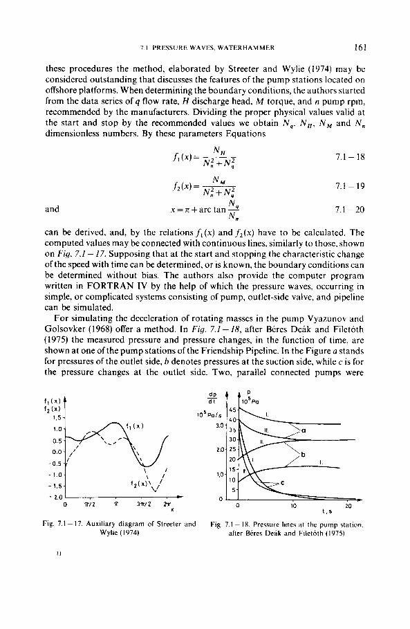
can be derived, and, by the relations f, (x) and f2(x) have to be calculated. The computed values may be connected with continuous lines, similarly to those, shown on Fig. 7.1 - 17. Supposing that at the start and stopping the characteristic change of the speed with time can be determined, or is known, the boundary conditions can be determined without bias. The authors also provide the computer program written in FORTRAN IV by the help of which the pressure waves, occurring in simple, or complicated systems consisting of pump, outlet-side valve, and pipeline can be simulated.
For simulating the deceleration of rotating masses in the pump Vyazunov and Golsovker (1968) offer a method. In Fig. 7.1 - 18, after Beres Deak and Filetoth (1975) the measured pressure and pressure changes, in the function of time, are shown at one of the pump stations of the Friendship Pipeline. In the Figure a stands for pressures of the outlet side, h denotes pressures at the suction side, while c is for the pressure changes at the outlet side. Two, parallel connected pumps were
0.5
0.0
-0.5
- - l S 0 l 1,s - 2.0 I c
0 T / Z P 3 W 2 h X
Fig. 7.1 - 17. Auxiliary diagram of Streeter and Wylie (1974)
0 10 20 t , s
Fig. 7.1 ~ 18. Pressure lines at the pump station. after Beres Delik and Filetoth (1975)
operating at the station. T.hc oil rate transportcd bq o n e pump is 3500 ni’ h, Lvhilc the two pumps topcthcr transported 4600 m3’h. The diagram w a s plottcd after thc stopping of o w pump. Before the measurements represented by c ~ i i vcs I ho!h pumps wcre in operation. while in ease ofcutvcs I / only one o f the pumps worked.
U p o n the centrifugal pumps both the pressure rise and the prcssurc depression caused by pressure w;i\,c may exercise ;I damaging cffect. ( i ) F‘irct of ;ill. i n case o f sinple suction pumps. the r:ipid change in pressure attempts to move thc impellers suddenly in the axiLil diiwtion and that may cituse serious damages. That is why the pumps of great capacity arc ofdouble suction type. ( i i ) The pressure wave arriving a t the pump station may c:iusc the r:ipid shut-down of the non-return valve. Due to this effect the fluid flow stops. the pump may be ovcrheatcd. the control stop\ the pump. and the damaging impact ofthe in-flowing pressure wave may increase. ( i i i ) I f the suction pressure. due to the depression decreases below the vapour pressure of the transported fluid. a vapour slug develops in the fluid, that getting i n t o the pump may cause cavitation damages.
The negative pressure wave causingcavitation occurs due to the sudden rise of the flow rate, that is provoked, e.g. by the starting of the preceding pump station, o r sudden opening of ii gate valve. Mostly, i t can be expected that the pipeline pressure sinks under the vapor pressure of the transported fluid. i f the depression wave propagates in the direction of the fluid flow. i.c. in the direction o f decreasing pressure. O n hilly terrains. in case of normal operation. the minimum pressures may be expected at the terrain peaks. The probability of the development of the vapour slugs, due to depression waves is the highest at these spots. Since. before the vapour slug, at the descending terrain section the flow velocity of the fluid is greater than at the ascending side. the volume of the vapour slug i s increasing for a time. Arriving in a section of greater pressure the slug "collapses". while the separated fluid masses flowing with different velocities of I , , and r 2 “crash”. The pressure rise
7.1 -21
at the moment of disappearing o f the cavity may be quite high. causing damages and leaks. A similar phenomenon may occur in the pump itself. The possibility of a depression wave m m t be always kept in mind at the suction side. when starting the pump operation.
Researchers, studying the laws of pressure waves, made an effort lately to represent graphically the pressure changes numerically determined previously by computers to facilitate the interpretation and location of this phenomenon. Techo (1976) describes a solution, at which the change of the pressure with length is printed, in the form of “letter-sketches”, by making use of the usual print-out equipment of computers. An even more up-to-date method is described by Jansen and Courage (1977). Here the pressure wave corresponding to the different operation and boundary conditions is displayed first on a display. then i t can be recorded in hard-copy form. By this method the operation of the designed oil- pipeline can be rapidly checked, and the most reliable solution can be selected.
7 2 S I UG TRANSPORTATION I63
7.2. Slug transportation
7.2.1. Mixing at the boundary of two slugs
The very same pipeline is often used for transporting several fluids of different quality in serial flow. The flowing fluid slugs, batches are mixing at the boundary developing between the two “pure” liquids, an increasing mixture slug during the flow. At one end of the interface the volumetric fraction of fluid A is c A = I , and this value, till the other end of the slug decreases to c A = O . The volumetric fraction of fluid B changes in the same way in the opposite direction. The mixing of the fluids raises difficulty both from the points of view of refining (if crude is transported), and of the utilization (if products are flowing in the pipeline). In each case, the allowed fraction cA.* that fluids A and B may contain from each other can be determined. In an extreme case this value may be even zero. Being aware of the features and the permitted utilization concentration of the mixed slug i t can be determined into which tank of the tank-farm belonging to the pipeline branches what quantity of pure, or mixed fluid should be directed. For crude transporting pipelines mixing means generally a smaller problem than for product transport. Knowledge of this phenomenon and its impact, however, is important in the first case, too.
The degree of mixing is significantly higher in case of laminar flow, as compared to the turbulent flow. The velocity distribution along the pipe-radius unam- biguously justifies this phenomenon. According to the derivation by Yufin (1976), in a given case (pipe radius =0.25 m; flow velocity = 1 m/s; friction factor =0.02) the value of the diffusion factor is higher by lo6 in case oflaminar than ofturbulent flow. Transporting slugs, generally turbulent flow must be used.
The basic computing problem of the slug flow is the determination of the length of the mixed, contaminated slug at given parameters. Several relations by different authors could be cited. I n the next section we introduce the essence of Weyer’s equation and ofits derivation based upon the works ofearlier authors(Weyer 1962). Weyer characterizes the turbulent mixing with the equation of the molecular diffusion. His starting point is the known diffusion equation
7.2- 1
where c is the concentration changing along the flow path; x is the fluctuating, axial displacement of a fluid particle in a long, straight pipe that can be described by the relation x = X - ut. Here X is the net axial displacement of the particle in t time after the start of the flow, while u is the average flow velocity and k d is the diffusion coefficient. The solution of the above differential equation is
7.2 - 2
164 7. PIPELINE TRANSPORTATION OF OIL
Y A
where by the interpretation y = ~ the second member of the right hand side of 2 J G
the formula from the relation
erf y = ~ e - y 2 dy f i o II:
on the basis of the Gauss-type error function can be computed. Let at one end of the interface the rate of A oil be e while that of the B oil be (1 - E). At the other end of the contaminated slug the rate of B oil is E, and that of the A oil is ( 1 - E). Supposing that c = 1 - E, where E = 0.95 and s = 2 x then
S erf ~
4 f i = 2 E - 1 7.2 - 3
Allowing the value E =0.95 theequation can be transformed into a simpler form and from this the length of the mixed slug is
s = 4 . 6 5 f i . 7.2-4
The kd diffusion factor was derived by Weyer on the basis of the turbulent velocity profile. He supposed that mass transfer takes place first of all in the radial direction. Due to the isotropic character of the turbulent flow, he also considered a mass transfer of smaller significance in axial direction, too. On this basis the diffusion factor is
where v , is the so-called frictional velocity that is the function of the shear stress, prevailing on the pipe wall, and the density:
The shear stress is
7.2 - 6
7.2 - 7
where 6 is the average flow velocity; 6= q/A. Substituting Eqs 7.2 - 6 and 7.2 - 7, and the relation r=di/2 into Eq. 7.2-5 we obtain
k d = 1.79 diii$. 7.2 - 8
This relation gives a shorter than real length for the mixed slug (Matulla 1972), and a theoretical mistake of the method is, that is neglects the increase of the mixing with the flow path. The relation offered by Austin and Palfrey (1963/64) seems to be more accurate. According to the authors the rate of the mixing, even in case of
7.2. SLUG TRANSPORTATION I65
turbulent flow, is significantly different above, and below of a critical value of N,, , . This critical value is given by the relation
- N~~~ = 104 f2 .7 .5% d , 7.2 - 9
Under the critical value the rate of mixing is greater and the length of the mixture can be calculated from equation
-
s = 18420(diL)0'5N,,0.9~2'19~d1 , 7.2- 10
while above the critical value it is obtained from relation
S = 11.75 (d iL)0 '5N,- ,0 '1 . 7.2- 1 1
For calculating the diffusion factor, Yufin (1976) describes several equations among which Asaturian's relation is
k, = 17.4 GN:L3 , 7.2- 12
where the average kinematic viscosity is obtained from equation
Subscript A denotes the higher, while B the lower viscosity fluids. Example 7.2- 1. Let us determine the mixed slug length in case of a pipeline of
di=305 mm and of 695 km length with the allowed value of ~ = 0 . 9 5 . In the pipe- line two light products whould be transported in serial flow slugs. The average kinematic viscosity of the two products is V-09 x lo -" mZ/s, the average flow velocity is V = 1.652 m/s, while the relative roughness of the pipe wall is k / d i = 2 x 10⁻⁴.
The Reynolds number is
The friction factor, from Eq. 1 . I - 7 is
on the basis of Eq. 7.2-8
/ id= 1.79 x 0.305 x 1.652 J m = 0 1 1 2 ,
and according to Eq. 7.2-4
=1009m. 1.652
I66 7. PIPELINE TRANSPORTATION OF OIL
The critical Reynolds number, calculated by applying the Austin and Palfrey equation is
__ N ~ ~ ~ = ]04,2.75vOo.305=4.57 x lo4.
Since 5-60 x 105>4.57 x lo4, the length of mixture can be computed from Eq. 7.2 - 11, i.e.
s = 11.75(0.305 x 695 x 103)0.5(5.60 x 10’)~o” = 1440m.
In practice, several phenomena, related to the mixing of oil slugs can be found, the previous simulation of which can be important. Emphasized items are as follows:
(i) Between the two slugs, already at the initial stage of the flow in the pipeline, mixed slug occurs. The reason for this fact can be different. ( 1 ) With change of the crude type, the opening and shut-down of the valves need a definite time, on this account the two fluids are mixed already at the initial stage. (2) In pipelines on hilly terrains, during the shut-down period, the liquid of greater density being at a higher level, may sink down. (3) If it is not allowed that the two liquids following each other mix, even to the slightest extent, then a dividing slug, made of liquid of allowable quality must be created. The numerical simulation of these cases is given by Frolov and Seredyuk (1974a, b). From his relations i t can be calculated that at a given time and determined spot what is the rate of mixing.
(ii) I t often occurs that fluid A of the slug stream is transported only to tanks being at a given end-point of one branch, while fluid B is to be transported to the tanks of the tank-farm at the end-point of the main pipeline. Through the mixed slug “contaminating” liquid gets into both end-point tanks. The quality of the stored fluids may deteriorate to a damaging level. Vladimirsky et a/. (1975) published a design method suitable to determine the concentration change of the mixed slug remaining in the pipeline. By applying this method the way of operation that prevents the undesirable quality deterioration may be planned.
(iii) If the flow is non-isothermal, the length of the mixed slug is greater than that of in case of isothermal flow. Chanisev and Nechval(1971) describe relations for the determination of mixing of oil slugs transported by spot heating.
(iv) The size of the mixed slug may be significantly influenced by the fluctuating velocity of the flow, the presence of the shut-down or open branches, and by-passes.
The length of the mixed section may be decreased if, between the two pure fluids, a dividing ball (so-called pipe-pig or gel slug) is applied (see Section 6.3). Their application, however, requires the building of proper input and output spots, and an other difficulty is raised by the passing through the booster pump stations (Matulla 1972). These dificulties may prove to be of small importance when because of the paraffin scraping input and output equipments are required, or, there is no booster pump station.
7.2.2. Scheduling of batch transport
If oil is carried in and out of the transport system in several places the design and optimization of the batch transport may be quite a complicated task. This applies especially to product transporting pipeline system carrying different products of several refineries to consumer centres (e.g. see Kehoe 1969). Scheduling a crude oil transporting system raises a smaller problem, since the fluid slugs to be transported here are relatively large, therefore the changes occur less frequently: the number of nodes in the pipeline system is generally smaller, and the transportation prescriptions are less rigorous. The scheduling procedure, however, is essentially the same as in the case of product pipeline system (Speur et uI. 1975).
The task of systems transporting crude, in case of continental countries basically is, that they should carry the crude from the oil fields to thc refineries. To this system lines of several oil fields may be joined, and through branching pipes the crude may be distributed among several refineries. If the quality of the crudes, originating from the different fields, is only slightly different regarding the hydraulic parameters of the transport and the requirements of the refineries, then, using prescribed parameters, the quantitative demands of the transportation must be satisfied only. If, however, the quality of the crudes to be transported from different fields significantly differs, and the crudes may not be transported in a mixture of homogeneous composition, then within the common transport sections slug transport is needed. Also, slug transport can be designed for pipelines, through which crudes of different qualities are transported from the shore-terminal to the refineries. The quality of the crudes, obtained on tankers, may differ from shipment to shipment.
There are three main design problems of the batch transport: a) the determination of the sequence of the slugs (batches) defined by the transport requirements; b) the numerical simulation of the flow; and c) the batch nomination sequencing.
First, generally monthly plans are prepared, considering the requirements of the consumers, and refineries, taking into account the available batches of the crude and using approximate flow and transport relations. On the basis of the above consideration the realizable monthly scheduling may be elaborated, that shows when, how many and what sort of crude should be injected into the system from different source points and at what time, what sort of and how much oil will be transported in different refineries. Scheduling for a shorter period, e.g. for a week or for ten days, can be carried out after this planning. At this stage already the hydraulic parameters of the transport system must be considered. This design process includes the solution of factual problems (which pump, when, from which tank and where should deliver; into which tank of the refinery what kind of crude, and at what time is pumped, etc.). Later on, the design is generally modified, since the real time of the injection of the crude batches, their volume may differ from the originally designed values, the pumps may fail, etc. By applying the parameters, differing from the designed ones, the operational plan must be modified in a very short time.
168 7. PIPELINE TRANSPORTATION OF 011.
If, even the fact is considered, that the problem of transportation must be solved, regarding not only the technical feasibility but also the transport costs, i.e. an optimum operation must be designed, it is obvious that it can only be realized by applying computers.
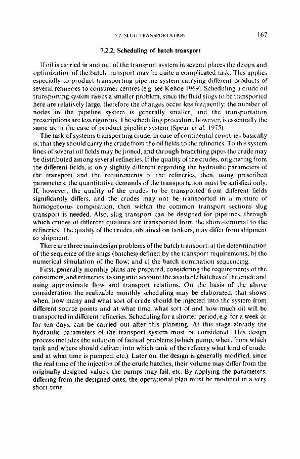
In DeFelice’s opinion (1976) the first problem to be solved by scheduling is the batch nomination sequencing. To each of the oil slug to be transported a code-name is given, that unambiguously expresses the shipper origin, source, product, grade, cycle requested and consignee of the volume specified. The first schedule is prepared by experimental relations obtained from the data of former transports. Several computerized design methods for precise hydraulic schedule are applied. One of these described by Techo (1976) is the so-called master-clock method. At this method a volume unit is taken, as the basis of the design, e.g. 1.5 m3. Within the system checking points are determined. These are the spots on the pipeline (control- points) where some operation influencing the transport process occurs (e.g. terminals, initial sections of branches, etc.). Starting from a given situation, the
al c e
a t , time
Fig. 7.2- 1. Rate v. time diagram of batch transport, after Techo and Holbrook (1974)
element which is the nearest to any control point is chosen, and the time needed for reaching this point is calculated. At this moment the position of the slug elements is fixed, in relation to the control points, and the calculation is going on by applying the previous method. This method is relatively rapid and flexible, but its disadvantage is that it does not calculate the movement of the slug boundaries. After Techo and Holbrook (1974), in case of a product pipeline, the complexity of the slug motion, is well illustrated by a three dimensional diagram shown in Fig. 7.2- I ,
1.2. SLUG TRANSPORTATION 169
where, in the function of time, the changes in the pump rates, at the pump stations are shown. Crosby and Baxter (1978) describe the main types of algorithms, on the basis of which computer programs are elaborated to increase the flexibility and capacity of the transporting system.
7.2.3. Detection of slug’s borders
To deliver the pure fluids and the mixed slug into the designed tanks, it is necessary that the dispatcher should be continuously informed about the position of the slug boundaries, about the distance of these from the tail end points, and branches of the pipeline. In case of computerized control, the computer, on the basis of the input data, obtained by on-line flow meters, continuously computes the movement of the boundaries, and their momentary position, and these data are either visually, or digitally transmitted to the dispatcher. This method, however, is generally not accurate enough f x controlling automated valve closing, or opening, and by these the transportation in proper direction and destination. That is why before the nodes of the pipelines, it is recommended to mount border detectors at given, predetermined intervals (e.g. distances of some 100 meters), and then at the occurrence of the change, signal is transmitted to the controlling centre, and/or, by on-line computer, valve openings and closures are automatically controlled. The boundary detector, in case of transporting without dividing device, directly measures the change in quality. Here, several methods are known. The instrument sensing the gamma irradiation and emission, indicates the change that, according to the oil qualities, the absorbed gamma-radiation, and thus the emitted radiation changes.
Zacharias (1969) describes an instrument operating on sonic principles. The sound velocity changes linearly with density. Into the oil, flowing in the pipeline, at certain intervals, sound impulses of great frequency are transmitted from the pipewall, and, between two previously determined surfaces, the propagation speed of the sound is measured. In case of two detectors method the dispatcher receives a warning signal while the slugborder passes the first detector, and the requested alteration in the direction of the flow is ordered while it passes the second detector. A density meter, complemented by simple comparator electronics, is also able to indicate slug boundaries.
Placing between the fluid slugs a dividing ball, perhaps pipe pig, the detectors show the passing of this device. By applying a mechanical dividing instrument, the rate of mixing can be reduced to 5 percent of the “without device” interface but the total prevention of this phenomenon is impossible. That is, the ball indicates the appearance of a fluid, the concentration of which may be determined by preceding calculations or tests. Changes in the flow direction should be ordered with this knowledge. For the detection, and signalling of the dividing ball, several methods were tested and applied. Yufin (1976) describes a mechanical signalling system. By the passing of the sphere a small cylinder penetrating radially into the pipeline is pushed out, and this signal is transmitted in an electric way. Speur and Jaques( 1977)
170 7. P I P E L I N E T R A N S P O R 7 A T I O N OF OIL
describe an ultrasonic dividing detector. Here, the perforation of the pipeline is not necessary. On the outside wall of the pipeline a transmitter, operating with piezo- crystal, is attached and ultrasonic signals continuously are transmitted through the pipe. The signals, arriving at the other side of the pipe, are sensed by a receiver. At the moment, when a mechanical dividing instrument moves in the section, measured by the'instrument, the intensity of ultrasonic signal significantly decreases. On this basis the dispatcher and/or the computer is informed about the passing of the fluid slug.
7.3. Leaks and ruptures in pipelines
Leaks, occurring in buried pipelines may be classified into two groups. The first group includes the big holes, caused by the rupture or break of the pipeline. They are mostly due to the too high internal pressure, or to external impact (earthquakes, landslides, the damaging operation of the bulldozers, etc.). I t may be also promoted by ruptures, or fault of the pipeline that remained undetected during hydrostatic pressure test. Through ruptures and breaks of this type a relatively large oil volume pours out from the pipeline within a short time. The second group includes small leaks that develop generally due to corrosion in a longer period of time. Through these leaks a relatively small oil rate seeps into the soil. Between the two groups, holes and outflow ofmean size practically do not occur (Kreiss 1972). Thus the main tasks of the leak detection are: (i) the checking of the integrity of the pipeline before starting its operation; (ii) the determination of the existence, and the locality of great leakages within a very short period of time; (iii) the recognition and location of small seepages, generally periodically. In the following section we discuss problems (ii) and (iii).
For the detection of the existence and the spot of the leaks in case of operating pipelines several methods have been elaborated. The most ancient method is the regular ranging over of the trace and its visual observation. Today, this operation is partly, or totally performed from vehicles (helicopters, planes). Particularly in case of great leaks and breaks the outpouring oil may cause considerable damages, that is why the aim is that the existence and locality of the rupture should be found in the shortest possible time after its induction. Beside the visual observation, systematic instrumental tests, and observation methods are also applied. Small leaks, caused by corrosion can be visually observed at the ranging only, if the seeping oil contaminates already the surface. In order to recognize the phenomenon in the shortest possible time the instrumental observation of this type of leakage should be also introduced. Table 7.3-1, after Takatsu, gives a survey of the instruments determining the existence, and sometimes also the place of the leaks. The symbols, used for the qualification are as follow: I to be applied in the first place; 2 is to be applied in the second place, or less suitable; 0 not suitable; + stands for instruments recommended in Japan; while - means that the device is officially not recommend- ed for application in Japan. In the following part some methods of major impor- tance are discussed. The interpretation of the type marks is shown on the Table.
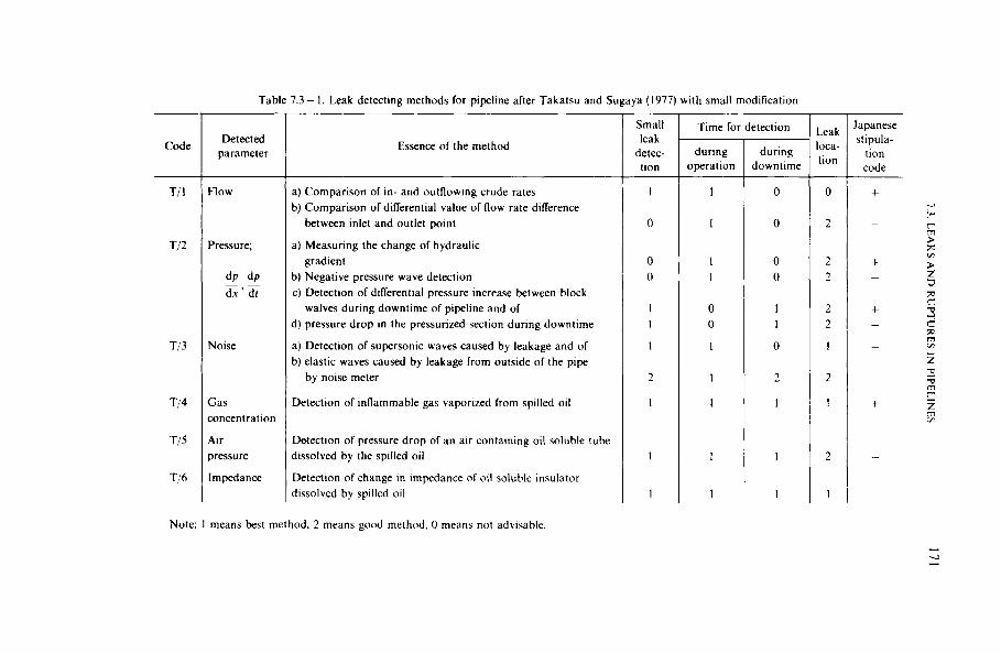
Table 7.3- 1. Leak detecting methods for pipeline after Takatsu and Sugaya (1977) with small modification
Code Detected
parameter
Flow
Pressure:
* d p dx ' dr
Noise
Gas concentration
Air pressure
Impedance
Essence of the method
a) Comparison of in- and outflowing crude rates b) Comparison of differential value of flow rate difference
between inlet and outlet point
a ) Measuring the change of hydraulic
b) Negative pressure wave detection c) Detection of differential pressure increase between block
d) pressure drop in the pressurized section during downtime
a) Detection of supersonic waves caused by leakage and of b) elastic waves caused by leakage from outside of the pipe
gradient
walves during downtime of pipeline and of
by noise meter
Detection of inflammable gas vaporized from spilled oil
Detection of pressure drop of an air containing oil soluble tube
dissolved by the spilled oil
Detection of change in impedance of oil soluble insulator dissolved by spilled oil
Small leak
detec- tion
1
0
0 0
1 I
I
2
1
1
1
Time for detection
during operation
1
I
1 I
0 0
1
1
1
1
1
during downtime
0
0
0 0
I 1
0
2
I
I
1
Leak loca- tion
0
2
2 2
2 2
I
2
I
2
I
Japanese stipula-
tion code
Note: I means best method. 2 means good method. 0 means not adviwble
172 7. PIPELINE TRANSPORTATION OF OIL
7.3.1. The detection of larger leaks
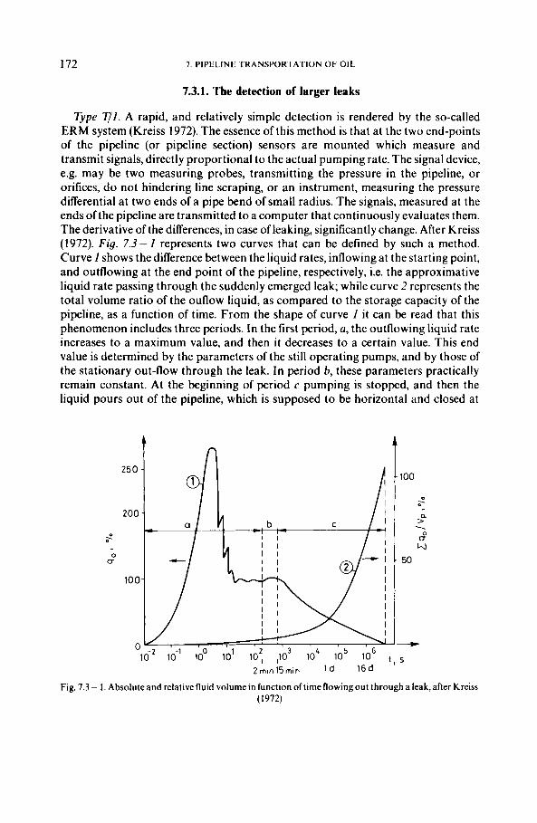
Type T / I . A rapid, and relatively simple detection is rendered by the so-called ERM system (Kreiss 1972). The essence of this method is that at the two end-points of the pipeline (or pipeline section) sensors are mounted which measure and transmit signals, directly proportional to the actual pumping rate. The signal device, e.g. may be two measuring probes, transmitting the pressure in the pipeline, or orifices, do not hindering line scraping, or an instrument, measuring the pressure differential at two ends of a pipe bend of small radius. The signals, measured at the ends of the pipeline are transmitted to a computer that continuously evaluates them. The derivative of the differences, in case of leaking, significantly change. After Kreiss (1972). Fig. 7.3-I represents two curves that can be defined by such a method. Curve I shows the difference between the liquid rates, inflowing at the starting point, and outflowing at the end point of the pipeline, respectively, i.e. the approximative liquid rate passing through the suddenly emerged leak; while curve 2 represents the total volume ratio of the ouflow liquid, as compared to the storage capacity of the pipeline, as a function of time. From the shape of curve I it can be read that this phenomenon includes three periods. In the first period, a, the outflowing liquid rate increases to a maximum value, and then it decreases to a certain value. This end value is determined by the parameters of the still operating pumps, and by those of the stationary out-flow through the leak. In period b, these parameters practically remain constant. At the beginning of period c pumping is stopped, and then the liquid pours out of the pipeline, which is supposed to be horizontal and closed at
C;" 7 2 -
250
200
2
0 U
100
0
n 100
. - a > . s Y
50
7.3. LEAKS A N D RUPTURES IN PIPELINES I73
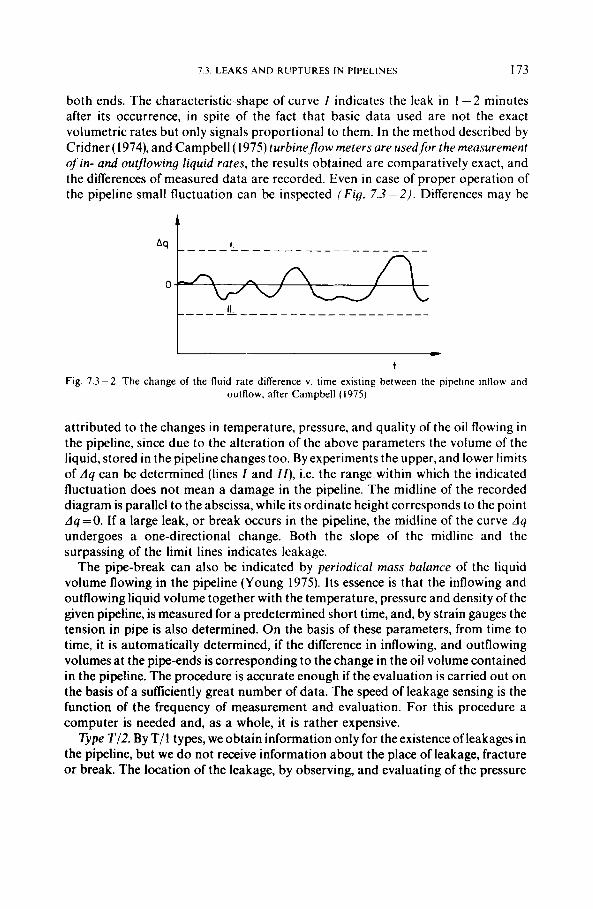
both ends. The characteristic shape of curve I indicates the leak in 1-2 minutes after its occurrence, in spite of the fact that basic data used are not the exact volumetric rates but only signals proportional to them. In the method described by Cridner (1974), and Campbell (1975) turbineflow meters are usedfor the measurement of in- and outflowing liquid rates, the results obtained are comparatively exact, and the differences of measured data are recorded. Even in case of proper operation of the pipeline small fluctuation can be inspected ( F i g . 7.3-2). Differences may be
- - - - - - - - - - - - - - - - - - - - - - - - - 3 t
Fig. 7.3-2. The change of the fluid rate dilTerence v. time existing between the pipeline inflow and outflow, after Campbell (1975)
attributed to the changes in temperature, pressure, and quality of the oil flowing in the pipeline, since due to the alteration of the above parameters the volume of the liquid,stored in the pipelinechanges too. By experiments the upper, and lower limits of A q can be determined (lines I and If), i.e. the range within which the indicated fluctuation does not mean a damage in the pipeline. The midline of the recorded diagram is parallel to the abscissa, while its ordinate height corresponds to the point A q = O . If a large leak, or break occurs in the pipeline, the midline of the curve A q undergoes a one-directional change. Both the slope of the midline and the surpassing of the limit lines indicates leakage.
The pipe-break can also be indicated by periodical mass balance of the liquid volume flowing in the pipeline (Young 1975). Its essence is that the inflowing and outflowing liquid volume together with the temperature, pressure and density of the given pipeline, is measured for a predetermined short time, and, by strain gauges the tension in pipe is also determined. On the basis of these parameters, from time to time, it is automatically determined, if the difference in inflowing, and outflowing volumes at the pipe-ends is corresponding to the change in the oil volume contained in the pipeline. The procedure is accurate enough if the evaluation is carried ou t on the basis of a sufficiently great number of data. The speed of leakage sensing is the function of the frequency of measurement and evaluation. For this procedure a computer is needed and, as a whole, it is rather expensive.
Type T/2. By T/1 types, we obtain information only for the existence of leakages in the pipeline, but we do not receive information about the place of leakage, fracture or break. The location of the leakage, by observing, and evaluating of the pressure
174 7. PIPELINE TRANSPORTATION OF OIL
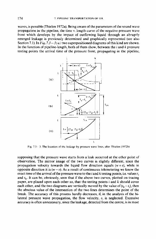
waves, is possible (Thielen 1972a). Being aware of the parameters of the sound wave propagation in the pipeline, the time v. length curve of the negative pressure wave front which develops by the impact of outflowing liquid through an abruptly emerged leakage is previously determined and graphically represented (see also Section 7.1). In Fig. 7.3 - 3 ( a ) two superpositioned diagrams of this kind are shown. In the function of pipeline-length, both of them show, between the i and k pressure testing points the arrival time of the pressure front, propagating in the pipeline,
t
+ 1
Fig. 7.3-3. The location of the leakage by pressure wave lines. after Thielen (1972b)
supposing that the pressure wave starts from a leak occurred at the other point of observation. The mirror image of the two curves is slightly different, since the propagation velocity towards the liquid flow direction equals ( w + u), while in opposite direction it is ( w - u ) . As a result of continuous telemetering we know the exact time of the arrival of the pressure wave to the i and k testing points, i.e. values ti and t , . It can be, obviously, seen that if the above two curves, plotted on tracing paper, are placed upon each other so, that the testing points i and k should cover each other, and the two diagrams are vertically moved by the value of ( tk - ti), then the abscissa value of the intersection of the two lines determines the point of the break. The accuracy of this process hardly decreases, if, in the analysis of the bi- lateral pressure wave propagation, the flow velocity, u, is neglected. Excessive accuracy is often unnecessary, since the leakage, detected from the centre, is in most
7.3 LEAKS A N D KUPTUKCS IN PIPELINES I75
cases seen by the service team sent to the spot, from distances of several hundred meters. In F i g . ( h ) is shown that, in practice, the location of the leakage, on the basis of the simplified curve, is performed by the help of the dashed line mirror curve. F i g . ic ) shows the possibility of further simplification. Here, the point of the break is the abscissa value of that curve-point whose ordinate value is O . S [ t , , / ( t , - t , ) ] .
I t can often be found that at certain sections of the pipeline oils of different quality are transported. Thus, it may occur that even between two pressure testing stations of the damaged pipe section, oil slugs of two different qualities flow. I n such a case, the time v. length diagrams of the pressure wave, for both oil qualities, must be separately determined. By these curves and applying the above process two hypothetical break points are determined. The real break point will fall between the two calculated values. Being aware of the approximate place of the slug boundary at the moment of the break, the curves, time v. length may be made more accurate and thus, the location, if it is necessary, can be improved.
I n spite ofthe fact that by applying the pressure wave method not only the place of leakage, but, obviously its occurrence may be also determined, the 7 1 1 processes are useful as well. The simultaneous application of different methods significantly increases the reliability of leak detection. In the Federal Republic of Germany, e.g., the simultaneous application of two independent methods is prescribed.
7.3.2. The detection of small leaks
Type 773. The oil flowing out of the pipeline through a small leak and seeping into the soil generates sound. The flow being turbulent, a high frequency ultrasound develops that may be detected by instruments. Depending on the fact whether the measurement takes place outside or inside of the pipe wall, two types of solutions are known. In the first case, the detection and simultaneously the location of the leak is carried out by the help of a contact microphone mounted on the outer surjiuce ofthe pipe wall sensing ultrasounds. Before the measurement, at certain points the soil is dug up and removed from the outside surface of the pipeline. If the leakage point is bracketed, then the next measurement is carried out at the midpoint between the two former test places. The first measurements were carried out by MAPCO in distances ranging from 1.2 - 9.6 km, and the accuracy of location was about 180 m (Pipe Line. . . 1973). In the other type of detection, pipe-pigs, pistons, moiling along together with the liquid stream are inserted into the line, that are suitable for observing and recording ultrasounds. The signals are recorded on magnetic tape. After the bringing out of the piston, the location may be carried out on the basis of recorded velocity data of the pipe-pi& and the recorded signals of outside mounted locators. In Karlsruhe, a significant amount of work was devoted to the determination of the conditions, among which, at the outflow of the oil through a small leak, ultrasonic signals of proper strengths can be obtained. I t has been established that the intensity of the sound significantly depends on the cavitation occurring at the outflow, and on the stream being turbulent or not. The applicability range of this process was also determined (Naudascher and Martin 1975).
176 7. PIPELINE TRANSPORTATION OF OIL
Type T/6. The “heart” of this process is an electric cable conducting alternating current. It consists of two metal wires insulated by a special material, soluble in oil. If this insulator is wetted by oil, or by any oil product, then it gets solved, the two metal wires get into contact, and by changing the resistance of the cable, in the monitor of the control station a warning signal appears. On the basis of the modified resistance, the leakage detector determines the distance where the short-circuit in the cable has taken place. The “Leak X” system, operating on the very same principle, is also suitable for indicating the damages caused by bulldozers (Hydrocarbon. . . 1973).
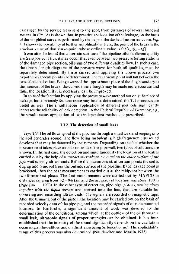
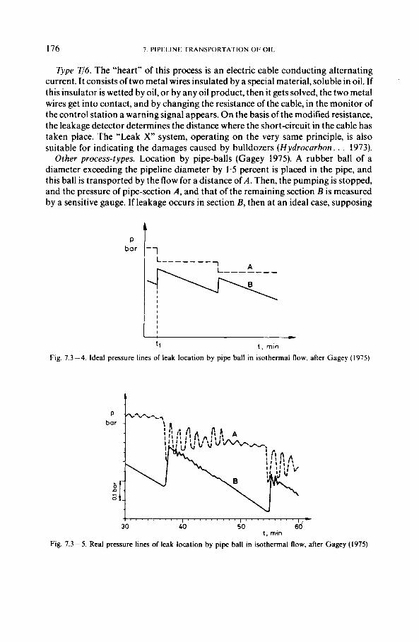
Other process-types. Location by pipe-balls (Gagey 1975). A rubber ball of a diameter exceeding the pipeline diameter by 1.5 percent is placed in the pipe, and this ball is transported by the flow for a distance of A. Then, the pumping is stopped, and the pressure of pipe-section A, and that of the remaining section B is measured by a sensitive gauge. If leakage occurs in section B, then at an ideal case, supposing
11 t , min
Fig. 7.3 -4. Ideal pressure lines of leak location by pipe ball in isothermal flow, after Gagey (1975)
+ 8 . . . . . . T 7 , . 1 - 1 1 . 1 1 1 , 3 1 1 1 1 . . . . - 30 40 50 €id
t , rnin
Fig. 7.3 - 5. Real pressure lines of leak location by pipe ball in isothermal flow, after Gagey (1975)
7.4. ISOTHERMAL O I L TRANSPORT I77
isothermal flow, pressure profiles, shown in Fig. 7.3-4 are obtained. Pumping stopped at moment t , . In section A the pressure remains unchanged, while in the section B it decreases continuously to the point, at which across the two sides of the ball a pressure differential of 0.1 -0.5 bar, required for the moving the ball develops. Then the ball starts to move, and after covering a short distance it stops again. Due to this ball displacement, pressure in section A slightly decreases, and then remains
bar P 1%
1 D
1 , min
Fig. 7.3 -6. Ideal pressure lines of leak location by pipe ball. after non isothermal flow (Gagey 1975)
constant. The pressure in section B, after a sudden, slight rise, decreases further continuously. In reality, due to the peculiar motion of the ball, getting stuck from time to time, the ideally straight pressure lines are modified. In Fig. 7.3-5 real, measured pressure lines are shown. If, before the stopping, flow was not isothermal, then the theoretical pressure lines are similar to those, shown in Fig. 7.3 -6. Because due to the cooling of the oil, the pressure in section A is also reduced. The rate of decrease in the pressure, however, is smaller here than in section B. If, after the first experiment, the ball is transported at a farther point of the pipeline, then other experiments, similar to the one described above, may be carried out, and so the spot of the leakage may be determined with an ever increasing accuracy. By this method even relatively small leaks can be well detected.
7.4. Isothermal oil transport
The temperature of the oil, flowing in a pipeline, generally varies along the length of the line. If, however, the viscosity of the crude is low, and the starting temperature does not significantly differ from soil temperature, then, for practical reasons, the flow may be considered isothermal.
7.4.1. Oil transportation with or without applying tanks
Main parts of the transporting system are the pipeline and the pump stations. If the oil is to be transported to a place located at a relatively small distance, then, one pump station at the head end point may prove to be sufficient. If, however, the pipeline is long then the building of several, so-called booster pump stations is
I 2
I78 7. PIPELINE TRANSPORTATION OF OIL
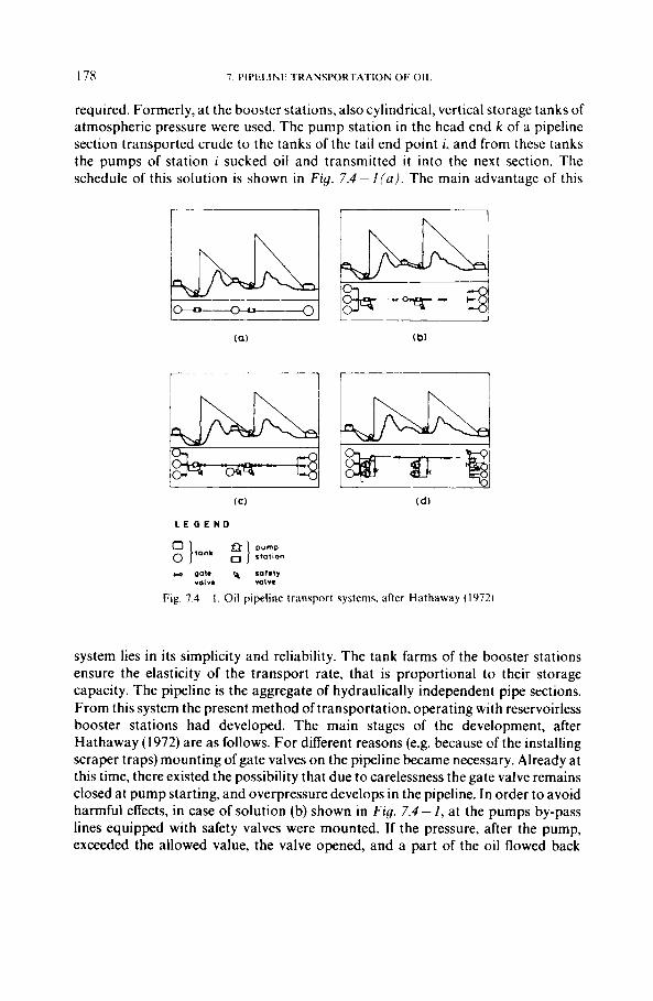
required. Formerly, at the booster stations, also cylindrical, vertical storage tanks of atmospheric pressure were used. The pump station in the head end k of a pipeline section transported crude to the tanks of the tail end point i, and from these tanks the pumps of station i sucked oil and transmitted it into the next section. The schedule of this solution is shown in Fig. 7.4-1fa). The main advantage of this
I 1
( C )
L E G E N D
w got. safely YOLY. valve
Fig. 7.4- 1 . Oil pipeline transport systems. after Hathaway (1972)
system lies in its simplicity and reliability. The tank farms of the booster stations ensure the elasticity of the transport rate, that is proportional to their storage capacity. The pipeline is the aggregate of hydraulically independent pipe sections. From this system the present method of transportation, operating with reservoirless booster stations had developed. The main stages of the development, after Hathaway (1972) are as follows. For different reasons (e.g. because of the installing scraper traps) mounting of gate valves on the pipeline became necessary. Already at this time, there existed the possibility that due to carelessness the gate valve remains closed at pump starting, and overpressure develops in the pipeline. In order to avoid harmful effects, in case of solution (b) shown in Fig. 7.4-1, at the pumps by-pass lines equipped with safety valves were mounted. If the pressure, after the pump, exceeded the allowed value, the valve opened, and a part of the oil flowed back
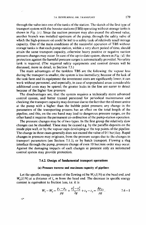
7.4. ISOTHERMAL OIL TRANSPORT 179
through the valve into one of the tanks of the station. The sketch of the first type of transport system with the booster stations (TBS) operating without storage tanks is shown in Fig. (c). Since the suction pressure may also exceed the allowed value, another branch was installed upstream of the pump, through the safety valve of which the high-pressure oil could be led to a safety tank of relatively small storage capacity. One of the main conditions of the successful operation of TBS without storage tanks is that each pump station, within a very short period of time, should attain the same transport capacity, otherwise heavy positive or negative suction pressure changes may occur. In case of the up-to-date system, shown in F i g . I d ) the protection against the harmful pressure surges is automatically provided. N o safety tank is required. (The required safety equipments and control devices will be discussed, more in detail, in Section 7.5.)
The main advantages of the tankless TBS are the following: the vapour loss during the transport is smaller; the system is less incendiary; because of the lack of the tank farm and its equipment the investment costs are significantly lower; it can work without personnel, and especially, in case of unpopulated areas considerable additional costs may be spared; the greater leaks in the line are easier to detect because of the higher line pressure.
The disadvantages are, that the system requires a technically more advanced control system, and better trained personnel for periodical maintenance and checking; the transport capacity may decrease due to the fact that the oil must arrive at the pump with a higher than the bubble point pressure; any change in the parameters of the transporting process has an effect on the total length of the pipeline, and this, on the one hand may lead to dangerous pressure surges, on the other hand it requires the permanent co-ordination of the pump-station operation.
The pressure changes may be of two types. In the first group the relatively slow changes can be classified. These may be caused e.g. by the parafin deposits on the inside pipe wall, or by the vapour caps developing at the top points of the pipeline. The change in these cases generally does not exceed the value of 0.1 bar/day. Rapid changes in pressure may originate, from the pressure surges due to the changes in transport parameters (see Section 7. l . l ) , or by batch transport. Flowing a slug interface through the pump, pressure change of even 10 bar/min order may occur. Against the damaging impacts of such changes in pressure only an automated control system may provide protection.
7.4.2. Design of fundamental transport operations
(a) Pressure traverse and maximum capacity of pipelines
Let the specific energy content of the flowing oil be W, ( J / N ) at the head end, and W,(J/N) at a distance of I, m from the head end. The decrease in specific energy content is equivalent to friction loss, i.e. it is
A P,x
P9 29 PY + z , -z,= ~
P I - P x v : - 4 w, - w, = ___ i - 7.4- 1
I80 7 PII’I 1 IN1 TKANSI’OKIATION 0 1 0 1 1
Let usexpresstheformula Ap/,/[~.(~ash/,,and substitute Eq. 1 . 1 - I tocxprcss A p r l . then we obtain
where the hydraulic. or friction gradient is
q
4
Substituting formula I:= --and the q=9.81 value we find that d fn
~~~~
7.4-- 2
7.4- 3
7.4 ~ 4
Each term of Eq. 7.4- 1 permits a twofold physical interpretation. They may be considered, on the one hand, as energy contents of a liquid body of unit weight, in J / N units, and on the other, as liquid column heights in m, the density of thc liquid being p .
The p / p g term the specific external potential energy is equivalent to pressure head h and the specific kinetic energy u 2 / 2 g to velocity head h,,. while the specific internal potential energy to the geodetic height, denoted by z. Neglecting the change in the specific volume of the flowing liquid, due to the change of pressure. in case of isothermal flow u 1 = u 2 , i.e. the velocity head difference between two pipeline cross sections is zero. I t means, that Eq. 7.4- 1 can be expressed in the following, simpler form:
7.4 - 5
In isothermal flow (/ is constant, and therefore the specific energy content of the flowing oil, along the pipeline linearly decreases along the pipeline. On horizontal terrains z1 =zz, and thus Eq. 7.4-5 is further simplified, as
WI - W, = hl - h, + ~ 1 - Z, = ( / I x .
h , = h , -tJ,, 7.4 - 6
i.e. the pressure head of oil, flowing in the pipeline, decreases linearly with distance along the pipeline.
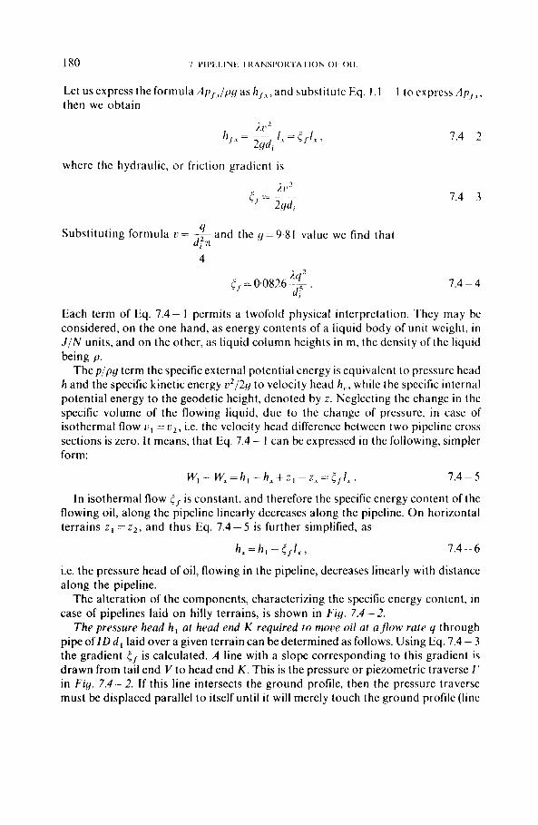
The alteration of the components, characterizing the specific energy content, in ease of pipelines laid on hilly terrains, is shown in Fig . 7 . 4 - 2 .
T h e pressure head h , at head end K required to mooe oil at af low rute q through pipe of ID d laid over a given terrain can be determined as follows. Using Eq. 7.4 - 3 the gradient r , is calculated. A line with a slope corresponding to this gradient is drawn from tail end V to head end K . This is the pressure or piezometric traverse I’ in Fig . 7 .4 -2 . I f this line intersects the ground profile, then the pressure traverse must be displaced parallel to itself until i t will merely touch the ground profile (line
7.4. ISOTHERMAL OIL TRANSPORT IS1
I ) . The initial pressure head h , is the above ground section of the ordinate at the head end K. It is recommended for satefy to augment h , by 30-50m, with due attention to the reliability of the basic data. The point M where the pressure traverse is tangent to the ground profile is called critical. This is where the pressure head of the flowing liquid is least. Hydraulic gradient is greater between points M and V than between K and M. Consequently, if there is no throttling at the tail end, flow is free beyond the critical point and oil will arrive at atmospheric pressure at the tail
h
102m I
20 30 , LO 50 60 70 l l , k m I '0
Fig. 7.4- 2. Pressure traverse of pipeline laid over a hilly terrain
end tank. If throttling is applied at the tail end, the oil will have a pressure head of h, at the end point: Vis usually above ground level, at the maximum possible liquid level of the tail-end tanks.
Another critical point as far as pipe strength is concerned may be valley point M'. I t is necessary to calculate the pressure head h above M and find out whether pressure p = hpg does not exceed the maximum allowable operating pressure of the pipeline. If the allowable pressure is exceeded, then pipes of greater wall thickness have to be applied or pressure reducing valves (see later) are to be installed.
Example 7.4-1. Let a pipeline of O D d,=219.1 mm and I D di=209.5mm (s =4.78 mm) be laid over the terrain shown in Fig. 7.1 -2. The throughput at the temperature of transportation is q = 150 m3/h; p = 830 kg/m3; v = 7.5 x 10 ~ m2/s; 1 = 72.4 km, and the equivalent roughness of the pipe is k =0.2 mm. Determine the pressure traverse and find the pump pressure p p .
The Reynolds number is
7.4 - 7 - od. 4 0.04167 N , , = = 1.273 - = 1.273
V di v 0.2095 x 7.5 x -
=3.38 x lo4.
1x2 7 PIPFI.INT. TRANSPORTATION OF 011
Pipe relative roughness:
k 2 x 1 0
d, 0.2095 ~ - - = 9 . 5 x 10⁻⁴ .
From the Colebrook formula (Eq . 1.1 -7) the friction factor is computed by iteration
By Eq. 7.4-4 the friction gradient
0.0253 x 0.04167'
0.20955 5 , = 0.00826 = 0.00899 m/m
The ordinate at K corresponding to the intercept of the pressure traverse traced backwards from Vaccording to Eq. 7.4- 5 is
17; = h,. + c r / - ( z K -2") = O + 0.00899 x 72 400 + 83 = 734 m . where 8.3 m is the geodetic-head difference ( z , - z 2 ) between point K and I/: In the Figure. the pressure traverse in question is shown by dashed line 1'. As it enters the ground. the head-end pressure head actually required is higher: i t is obtained by displacing the pressure traverse parallel to itself. making it tangent to the ground profile at the point M . Accordingly h; = 800 m. For safety, let us augment this by 40 m, giving h, = 800+40= 840 m. The pressure head of the pump to be installed at point K should then, be
pp = h K p ~ = 840 x 830 x 9.8 1 = 6.84 M Pa
Assuming that p u m p i n g station c..ui.sts only at K head end. rho qrratrst throughput qfrhe pipc l ine can be determined by the following procedure. Let us plot above the ground profile at K the pressure head h,,, corresponding to the maximum allowable operating pressure ofthe pipe ( F i g . 7.4-2). Joining this point with V (or with critical point M , if there is one) we obtain a pressure traverse whose slope corresponds to the maximum feasible pressure gradient i,-Omax. In the knowledge of this latter, the maximum oil throughput, qoma, can be determined as follows.
Let the two constants in Eq. 1.1 - 10 be a=O.194 and h=0.189. Then
i. = 0.194Ni;" '') . 7.4 - 8
Introducing this into Eq. 7.4-4
7.4 - 9
7.4- 10
whence
7.4. ISOTHERMAL OIL TRANSPORT I83
Introducing into Eq. 7.4 - 10 the graphically determined value of t,om;rx = 5, we may calculate qomax =q, the maximum liquid throughput of the pipeline if the only pump station is at the head end. The accuracy of the computation can be increased of the value of the friction factor, obtained from Eq. 7.4 - 8, is only considered as first approximation, and then the computation is continued by applying Eq. 1 . 1 - 7, i.e. the Colebrook formula. Eq. 7.4-4, similarly to the above by substituting the relation u - q, and the y = 9.81, respectively, may be simplified to the following form:
7.4- 1 I
where subscript a refers to the above calculated approximate values. Knowing the value qa a more accurate Reynolds number, and from the Colebrook formula 1.1 - 7 a more accurate AC friction factor can be computed. From Eq. 7.4 - I 1 i t follows that
&q: = R,q:
2.q: = 12.1 <,d;5 ,
and from this relation the more accurately determined flow rate is
7.4- 12
The exact qomax value is obtained after further iterations. Example 7.4 - 2. Let us find the maximum throughput of the pipeline
characterized in Example 7.4- I , if API standard pipe made of X-42 steel is used, and terrain belongs to category (a) characterized in Section 6.1 - 3, that is, the safety factor k = 1.3; let e = 1. The pressure rating is calculated using Eq. 6.1 ~ 3. From Table 6.1 - 3, aF = 289 M Pa, and hence by Eq. 6.1 - 2
289 1.3
aa,= ~ =222 x lo6 Pa
The maximum allowable internal overpressure is
A p - 9.69 x 10' pg 8 3 0 ~ 9 . 8 1
h;,,= - - =1190m.
Let us reduce this value by 40m for safety. Hence, h,,,= 1190-40= ll5Om. Plotting h,,, at the point K and joining it with V we get pressure traverse 11. Clear- ly, the pressure traverse passes above the critical ground-profile section, and the safety reserve of pressure is sufficient also from this point of view. The maximum pressure gradient is
1150-83 72 400
= 0.0 147 m/m 5,omax =
184 7. PIPELINE TRANSPORTATION OF 0 1 1
The maximum liquid throughput by Eq.7.4- 10 is
0.0147°'552 x 0.2095*"" = 0.0525 m3/s = (7.5 10 ~ (y I 04
qomar = = 10.1
= 189 m3/h.
Considering Eq. 7.4-7, the Reynolds number based on this pumping rate is
= 4 a x 104 0.0525
N , , = 1.273 0.2095 x 7.5 x 10
By Eq. 7.4 - 8
A,=0194 ~ ( 4 . 2 5 x lo4) 0"89=0.0259
and according to Eq. 1.1 - 7
From this relation, by applying a short iteration we obtain that
A, = 0.0243
By Eq. 7.4- 12
qi = 0.0522 ~ = 0,0539 m3/s = 194 m'/h . JZ If, at this rate, we calculate again N , , , and then 1,. then we receive the previous 0.0243 value, i.e. qi = qomax .
(b) Increasing the capacity of pipelines by looping
Even the maximum throughput qomax of an existing pipeline may be insufficient to transport the required qo rate. One of the possibilities to increase the transport capacity of the existing pipe line is looping: a second line, a so-called twin line is laid alongside the original pipeline and is jointed to it. The twin line may be of two types: (i) new line of same length as old line but usually of different diameter (complete loop), (ii) new line shorter than old line but of the same ID (partial loop). Exceptionally, pipelines, that are shorter than the original ones, but are of greater internal diameter, are applied. The advantage of the shorter twin line of different diameter, as compared to the full length twin line, is that the transfer capacity of the system, by way of increasing its length may be further increased.
Solution (i) may be regarded as two independent pipelines with the size ofthe new line chosen so as to deliver a flow of q2 = q , - qomax under the original input pressure h,,, between the points K and V Owing to the identity of trace and of input and
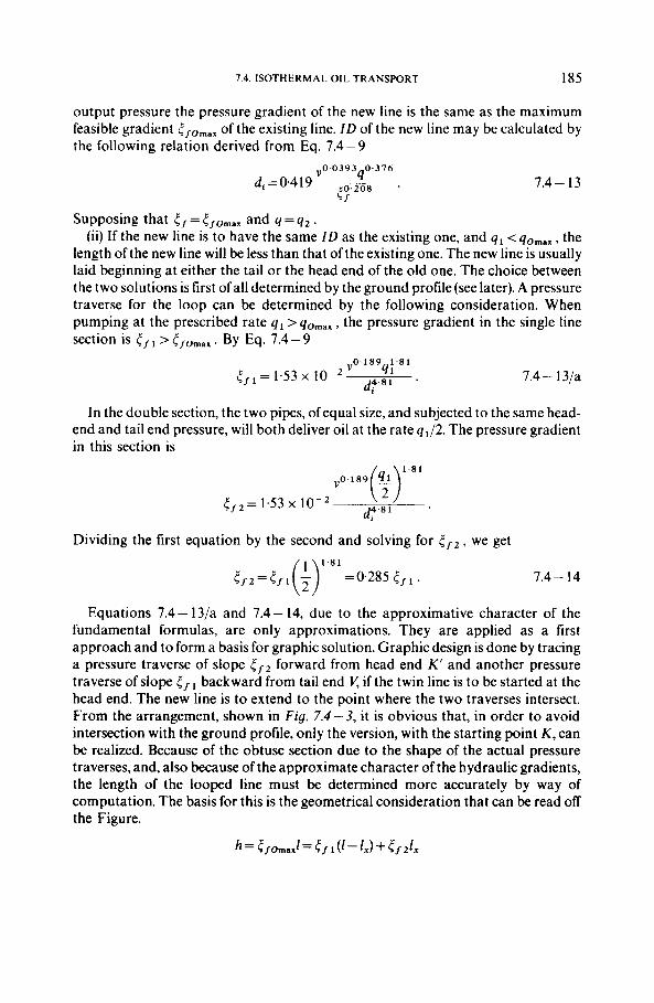
7.4. ISOTHERMAL OIL TRANSPORT 185
output pressure the pressure gradient of the new line is the same as the maximum feasible gradient (/Omax of the existing line. ID of the new line may be calculated by the following relation derived from Eq. 7.4-9
" 0 . 0 3 9 3 0 . 3 7 6 4 di=0-419 o,208
l / 7.4- 13
Supposing that 5 = 5 ,-Omax and q = q2 . (ii) If the new line is to have the same ID as the existing one, and q 1 <qomax, the
length of the new line will be less than that of the existing one. The new line is usually laid beginning at either the tail or the head end of the old one. The choice between the two solutions is first ofall determined by the ground profile (see later). A pressure traverse for the loop can be determined by the following consideration. When pumping at the prescribed rate q l >qomax, the pressure gradient in the single line section is 5 > 5 fOmax . By Eq. 7.4 - 9
v 0 . 1 8 9 1 .81
7.4 - 13/a
In the double section, the two pipes, of equal size, and subjected to the same head- end and tail end pressure, will both deliver oil at the rate q1/2. The pressure gradient in this section is
41 5, 1 = 1.53 x d4.81 .
Dividing the first equation by the second and solving for rf 2 , we get 1.81
5 / 2 = 5 / l(;) = 0.285 5, I 7.4- 14
Equations 7.4- 13/a and 7.4- 14, due to the approximative character of the fundamental formulas, are only approximations. They are applied as a first approach and to form a basis for graphic solution. Graphic design is done by tracing a pressure traverse of slope tf forward from head end K' and another pressure traverse of slope 5 backward from tail end V , if the twin line is to be started at the head end. The new line is to extend to the point where the two traverses intersect. From the arrangement, shown in Fig. 7.4-3, it is obvious that, in order to avoid intersection with the ground profile, only the version, with the starting point K, can be realized. Because of the obtuse section due to the shape of the actual pressure traverses, and, also because of the approximate character of the hydraulic gradients, the length of the looped line must be determined more accurately by way of computation. The basis for this is the geometrical consideration that can be read off the Figure.
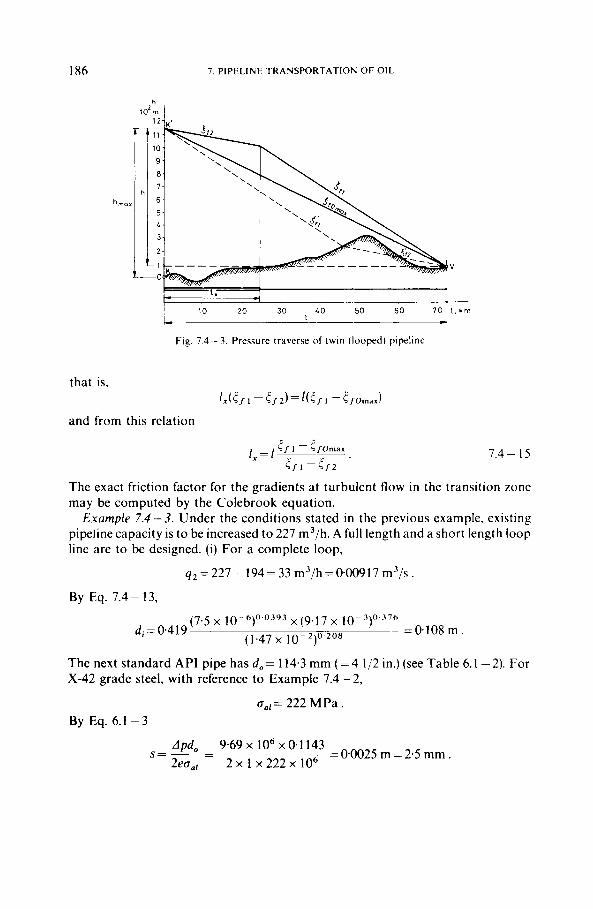
186 7. PIPELINE TRANSPORTATION OF OIL
- Fig. 7.4~- 3. Pressure traverse of twin (looped) pipeline
and from this relation
5 f I - 5 fOmax
t f l - r f z
1, = 1 7.4 - 15
The exact friction factor for the gradients at turbulent flow in the transition zone may be computed by the Colebrook equation.
Example 7.4 -3 . Under the conditions stated in the previous example, existing pipeline capacity is to be increased to 227 m3/h. A full length and a short length loop line are to be designed. (i) For a complete loop,
q2 = 227- I94 = 33 m3/h =O.O0917 m3/s.
By Eq. 7.4- 13,
(7.5 x 10⁻⁶)0.0393 x(9.17 x 10-3)0.376 ( 1 . 4 7 ~ 10-2)o'208
=0.108 m d ; = 0.4 1 9
The next standard API pipe has do= 114.3 mm ( = 4 1/2 in.) (see Table 6.1 -2). For X-42 grade steel, with reference to Example 7.4 - 2,
on,= 222 M P a . By Eq. 6.1 - 3
dpd, s= - - - 2eanr
9.69 x lo6 x 0.1 143 2 x 1 x 222 x lo6
= 04025 m = 2.5 mrn
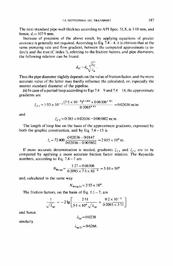
7.4. ISOTHERMAL OIL TRANSPORT 187
The next standard pipe-wall thicknes according to API Spec. 5LX, is 3.18 mm, and hence, di = 107.9 mm.
Increase of precision of the above result, by applying equations of greater accuracy is generally not required. According to Eq. 7.4 - 4, it is obvious that at the same pumping rate and flow gradient, between the computed approximate (a in- dex!), and the true (C index !), referring to the friction factors, and pipe diameters, the following relation can be found:
Thus the pipe diameter slightly depends on the value of friction factor, and the more accurate value of the latter may hardly influence the calculated, or, especially the nearest standard diameter of the pipeline.
(ii) In case of a partial loop according to Eqs 7.4 - 9 and 7.4 - 14, the approximate gradients are
(7.5 x 10⁻⁶)0.'89 x 006306"81 0.20954'81
= 0.02036 m/m = 1.53 x
and 5 , = 0.285 x 0.02036 = 0.005802 m/m .
The length of loop line on the basis of the approximate gradients, expressed by both the graphic construction, and by Eq. 7.4 - 15 is
0.02036 - 0.0 147 0.02036 - 0.005802
I , = 72 400 =2.815 x 10⁴m.
If more accurate determination is needed, gradients and t f 2 are to be computed by applying a more accurate friction factor relation. The Reynolds numbers, according to Eq. 7.4 - 7 are
= 5.10 x 10⁴ 1.27 x 0.06306
NRe(q)= 0.2095 x 7.5 x 10-
and, calculated in the same way
N R e ( q , 2 ) = 2.55 x lo4 .
The friction factors, on the basis of Eq. 1.1 -7, are
and hence
similarly = 00238
= 0.0266 .
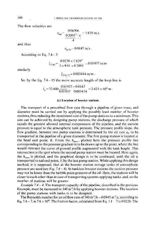
I88 7. PIP l : l . INl~ TKANSI'OK'IATION Ot- 0 1 1
The flow velocities are
and thus 4
~ 1 , ~ ~ ~ ) = 0.9 I 47 m/s
According to Eq. 7.4 - 3
0.0238 x 1.8292 2 x 9.8 I x 0,2095
= 0.0 I937 m/m c / w = ~~ ~~ ~
similarly t fIq ,,=0.005414 m/m.
/ So, by the Eq. 7.4- 15 the more accurate length of the loop line is
0.01937 -0.0147 0.0 1 937 - 0,0054 1 4
I , = 72 400 ~~~ ~~ ~ = 2.423 x lo4 m .
(c) Location of booster stations
The transport of a prescribed flow rate through a pipeline of given trace, and diameter must be carried out by applying the possibly least number of booster stations, thus reducing the investment cost ofthe pump stations to a minimum. This aim can be achieved by designing pump stations, the discharge pressure of which equals the greatest allowed internal overpressure of the pipeline, and the suction pressure is equal to the atmospheric tank pressure. The pressure profile slope, the flow gradient, between two pump stations is determined by the oil rate 4 , to be transported in the pipeline of a given diameter. The first pump station is located at the head end point, K . From the h,, , , plotted here the pressure profile line corresponding to the pressure gradient is to be drawn up to the point, where the line would intersect the curve of ground profile augmented with the tank height. This intersection is the spot where the second pump station must be located. Here again, the h,,, is plotted, and the graphical design is to be continued, until the oil is transported to tail end point, r! by the last pump station. While applying this design method, i t is supposed, that at the booster station storage tanks of atmospheric pressure are used (see Fig. 7.4-4). At tankless booster stations the suction pressure may not be lower than the bubble point pressure of the oil. Here, the stations will be closer to each other than in ease of transporting systems applying tanks, and, so the number of stations will be greater.
Example 7 .4- 4 . The transport capacity of the pipeline, described in the previous Example, must be increased to 340 m3/h by applying booster stations. The location of the pump stations with tanks is to be designed.
The Reynolds number for an oil flow rate of 340 m3/h =0.0945 m3/s, according to Eq. 7.4- 7, is 7.6 x lo4. The friction factor, calculated from Eq. 1 . I - 7 is 0.0226. The
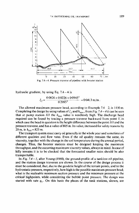
7.4. ISOTHERMAL OIL TRANSPORT 189
h
10'm I
10 20 30 40 50 60 70 l,km
Fig. 7.4 -4. Pressure traverse of pipeline with booster station
hydraulic gradient, by using Eq. 7.4-4 is
0.0826 x 0.0226 x 0.09452 0.20955
= O W 3 m/m. r / = ~
The allowed maximum pressure head, according to Example 7.4 - 2, is 1 150 m. Completing the design by using values of ( / and h,,, , from Fig. 7.4 - 4 i t can be seen that at pump station / I / the h,,, value is needlessly high. The discharge head required can be found by tracing a pressure traverse backward from point in which case the head in question is the height difference between the point / / I and the pressure traverse, and has a value of 805 m. Its value, increased for safety reasons by 20 m, is h,,, = 825 m.
The transport system must carry oil generally in the whole year and sometimes of different qualities and flow rates. Even if the oil quality remains the same, its viscosity, together with the change in the soil temperature during the annual period, changes. Thus, the booster stations must be designed keeping the maximum throughput, and the occurring maximum viscosity values, always in mind. In case of hilly terrains it is to be checked that the forecasted smaller rates should be also transportable.
In Fig. 7.4-5, after Young (1960), the ground-profile of a tankless oil pipeline, and the station design traverses are shown. In the course of the design process it must be considered, that, due to the geodetic height of the terrain points, and to the hydrostatic pressure, respectively, how high is the possible maximum pressure head; what is the realizable minimum suction pressure and the minimum pressure at the critical highpoints, while considering the bubble point pressure. The design was started with rate q l . On this basis the places of the tank stations, shown, are
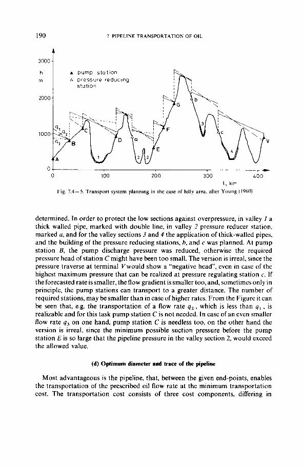
190 7. PIPELINE TRANSPORTATION OF OIL
0 . -
100 200 300 400 I , km
Fig. 7.4- 5 . Transport system planning in the case of hilly area, after Young ( 1960)
determined. In order to protect the low sections against overpressure, in valley I a thick walled pipe, marked with double line, in valley 2 pressure reducer station, marked a, and for the valley sections 3 and 4 the application of thick-walled pipes, and the building of the pressure reducing stations, b, and c was planned. At pump station B, the pump discharge pressure was reduced, otherwise the required pressure head of station C might have been too small. The version is irreal, since the pressure traverse at terminal Vwould show a “negative head”, even in case of the highest maximum pressure that can be realized at pressure regulating station c. If the forecasted rate is smaller, the flow gradient is smaller too, and, sometimes only in principle, the pump stations can transport to a greater distance. The number of required stations, may be smaller than in case of higher rates. From the Figure it can be seen that, e.g. the transportation of a flow rate q 2 , which is less than 4 , , is realizable and for this task pump station C is not needed. In case of an even smaller flow rate q3 on one hand, pump station C is needless too, on the other hand the version is irreal, since the minimum possible suction pressure before the pump station E is so large that the pipeline pressure in the valley section 2, would exceed the allowed value.
(d) Optimum diameter and trace of the pipeline
Most advantageous is the pipeline, that, between the given end-points, enables the transportation of the prescribed oil flow rate at the minimum transportation cost. The transportation cost consists of three cost components, differing in
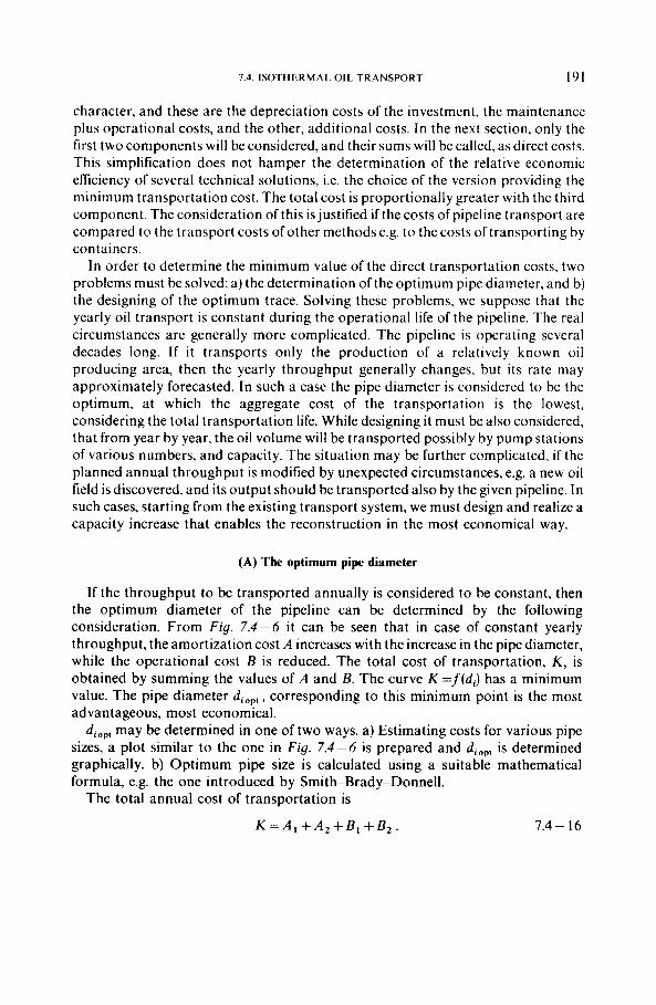
7.4. ISOTHERMAL OIL TRANSPORT 191
character, and these are the depreciation costs of the investment? the maintenance plus operational costs, and the other, additional costs. In the next section, only the first two components will be considered, and their sums will be called, as direct costs. This simplification does not hamper the determination of the relative economic efficiency of several technical solutions, i.e. the choice of the version providing the minimum transportation cost. The total cost is proportionally greater with the third component. The consideration of this is justified if the costs of pipeline transport are compared to the transport costs of other methods e.g. to the costs of transporting by containers.
In order to determine the minimum value of the direct transportation costs, two problems must be solved: a) the determination of the optimum pipc diameter, and b) the designing of the optimum trace. Solving these problems, we suppose that the yearly oil transport is constant during the operational life of the pipeline. The real circumstances are generally more complicated. The pipeline is operating several decades long. If i t transports only the production of a relatively known oil producing area, then the yearly throughput generally changes, but its rate may approximately forecasted. In such a case the pipe diameter is considered to be the optimum, at which the aggregate cost of the transportation is the lowest, considering the total transportation life. While designing it must be also considered, that from year by year, the oil volume will be transported possibly by pump stations of various numbers, and capacity. The situation may be further complicated, if the planned annual throughput is modified by unexpected circumstances, e.g. a new oil field is discovered, and its output should be transported also by the given pipeline. In such cases, starting from the existing transport system, we must design and realize a capacity increase that enables the reconstruction in the most economical way.
(A) The optimum pipe diameter
If the throughput to be transported annually is considered to be constant, then the optimum diameter of the pipeline can be determined by the following consideration. From Fig. 7.4-6 it can be seen that in case of constant yearly throughput, the amortization cost A increases with the increase in the pipe diameter, while the operational cost B is reduced. The total cost of transportation, K, is obtained by summing the values of A and B. The curve K =f(di) has a minimum value. The pipe diameter diop,, corresponding to this minimum point is the most advantageous, most economical.
diop, may be determined in one of two ways. a) Estimating costs for various pipe sizes, a plot similar to the one in Fig . 7 .4 -6 is prepared and diop, is determined graphically. b) Optimum pipe size is calculated using a suitable mathematical formula, e.g. the one introduced by Smith-Brady-Donnell.
The total annual cost of transportation is
K = A , + A 2 + B 1 + B 2 . 7.4- 16
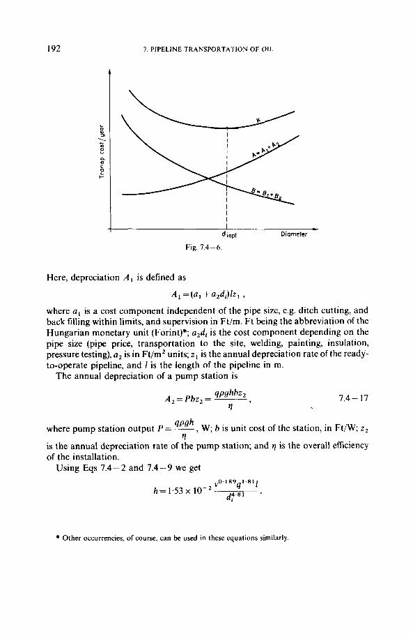
I92
-
7. PIPELINE TRANSPORTATION OF OIL
I I I -
Here, depreciation A , is defined as
where a, is a cost component independent of the pipe size, e.g. ditch cutting, and back filling within limits, and supervision in Ft/m. Ft being the abbreviation of the Hungarian monetary unit (Forint)*; azdi is the cost component depending on the pipe size (pipe price, transportation to the site, welding, painting, insulation, pressure testing), a, is in Ft/mz units; z , is the annual depreciation rate of the ready- to-operate pipeline, and 1 is the length of the pipeline in m.
The annual depreciation of a pump station is
7.4 - 17
where pump station output P = ~ 4 P g h , W; b is unit cost of the station, in Ft/W; zz
is the annual depreciation rate of the pump station; and 17 is the overall efficiency of the installation.
17
Using Eqs 7.4-2 and 7.4-9 we get yo.189 1.81
4 1 h = 1 . 5 3 ~ lo-’ d 4 , 8 1 .
Other occurrencies, of course, can be used in these equations similarly.
7.4. ISOTHERMAL OIL TRANSPORT I93
Substituting this into Eq. 7.4- 17 we find
7.4- 18
The annual operating cost is
B, = Pcef,
where c is the operating time over the year in s; r is the specific energy consumption (J/J for electric motors and kg/J for internal compustion engines);/is the unit price of power, or fuel (expressed in Ft/J, or Ft/kg).
Using the symbols introduced when deriving Eq. 7.4- 18 we obtain
7.4- 19
The annual cost of maintenance B2 may be considered constant. Let us replace the terms on the right-hand side of Eq. 7.4- 16 by the above-defined expressions, and determine the derivative dK/d(dJ. Putting the obtained relation equal to zero, and solving for the diameter we get, by the rules of calculus the pipe size that ensures the least cost of transportation
7.4 - 20
In calculating optimal pipe size we have so far tacitly assumed the pipeline to operate without interruption, that is, at 100 percent exploitation. In reality, transportation is most often intermittent to a greater or lesser degree. The pauses in transportation provide the flexibility needed to handle excess output due to non- uniform production, breakdown etc., on the input side. A lower exploitation efficiency will, however, augment the specific cost of transportation. Transportation costs may be analyzed for various (constant) pipe sizes and variable throughput. Let us replace by the above defined expressions the terms of the right-hand side of Eq. 7.4- 16. Let us contract the coefficients except di and 4 into constants denoted Ci; then we obtain relation
K = C , + C2di + C,di 4'8192'8' .
Let the length of the line be one km, and let us divide both sides ofthe equation by the annual oil throughput, C'qp. Let K / C ' q p = k denote the unit cost of transportation in Ft/(kg km) then
k=C4q- '+C5diq- '+C 6 i d - 4 ' 8 1 4"81 ' 7.4-21
The relationship defines a set of curves, k =f(4)di. The set in Fig. 7.4 - 7 has been plotted, using a similar relationship. The ordinate is calibrated in terms of a relative specific transportation cost kre, referred to some base value (derived from a diagram
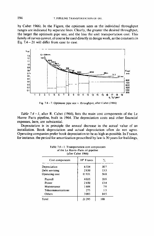
194 7. PIPELINE TRANSPORTATION OF- OIL
d,-508rnm
I I I I I 1 I , I I I
b’’‘&L
711 2 6801 Ma6
l t 2 m 658 @
I 1
I I I I I
762 mm , I
I I I I 1 I
I I r I I
I
I ! 1 7
I :-p I , I
, I #
!
by Cabet 1966). In the Figure, the optimum sizes in the individual throughput ranges are indicated by separate lines. Clearly, the greater the desired throughput, the larger the optimum pipe size, and the loss the unit transportation cost. This family ofcurves cannot, ofcourse be used directly in design work, as the constants in Eq. 7.4 - 21 will differ from case to case.
d,opI m m
.a00 ~. 700 .600 . 600 . 600 300
Cost components
Fig. 7.4-7. Optimum pipe size v. throughput, after Cabet (1966)
10” Francs %
Table 7.4-1, after R. Cabet (1966), lists the main cost components of the Le Havre-Paris pipeline, built in 1964. The depreciation costs and other financial expenses, here, are substantial.
Depreciation is in principle the annual decrease in the actual value of an installation. Book depreciation and actual depreciation often do not agree. Operating companies prefer book depreciation to be as high as possible. In France, for instance, the period for amortization prescribed by law is 30 years for buildings,
Depreciation Debt servicing Operating cost
Payroll Power Maintenance Telecommunications Others
Total
6 534 2 830
I 1 931
4 035 2 850 1688
275 3 083
21 295
30.7 13.3 56.0
18.9 13.4 7.9 1.3
14.5
100
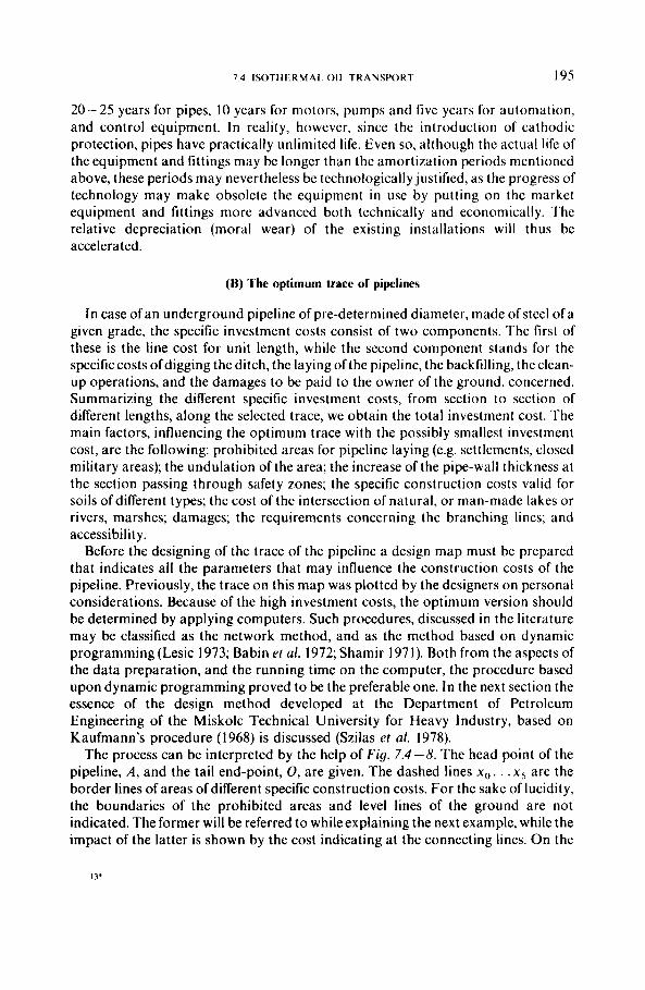
7 4 ISOTHLKMAI 011 TKANSI’OKT I95
20-25 years for pipes, 10 years for motors, pumps and five years for automation, and control equipment. In reality, however, since the introduction of cathodic protection, pipes have practically unlimited life. Even so, although the actual life of the equipment and fittings may be longer than the amortization periods mentioned above, these periods may nevertheless be technologically justified, as the progress of technology may make obsolete the equipment in use by putting on the market equipment and fittings more advanced both technically and economically. The relative depreciation (moral wear) of the existing installations will thus be accelerated.
(B) The optimum trace of piplines
In case of an underground pipeline of pre-determined diameter, made of steel of a given grade, the specific investment costs consist of two components. The first of these is the line cost for unit length, while the second component stands for the specificcosts ofdigging the ditch, the laying of the pipeline, the backfilling, the clean- up operations, and the damages to be paid to the owner of the ground, concerned. Summarizing the different specific investment costs, from section to section of different lengths, along the selected trace, we obtain the total investment cost. The main factors, influencing the optimum trace with the possibly smallest investment cost, are the following: prohibited areas for pipeline laying (e.g. settlements, closed military areas); the undulation of the area; the increase of the pipe-wall thickness at the section passing through safety zones; the specific construction costs valid for soils ofdifferent types; the cost of the intersection of natural, or man-made lakes or rivers, marshes; damages; the requirements concerning the branching lines; and accessibility.
Before the designing of the trace of the pipeline a design map must be prepared that indicates all the parameters that may influence the construction costs of the pipeline. Previously, the trace on this map was plotted by the designers on personal considerations. Because of the high investment costs, the optimum version should be determined by applying computers. Such procedures, discussed in the literature may be classified as the network method, and as the method based on dynamic programming(Lesic 1973; Babin et al. 1972; Shamir 1971). Both from the aspects of the data preparation, and the running time on the computer, the procedure based upon dynamic programming proved to be the preferable one. In the next section the essence of the design method developed at the Department of Petroleum Engineering of the Miskolc Technical University for Heavy Industry, based on Kaufmann’s procedure (1968) is discussed (Szilas et a/. 1978).
The process can be interpreted by the help of F i g . 7 .4-8. The head point of the pipeline, A , and the tail end-point, 0, are given. The dashed lines xo. . . x5 are the border lines of areas of different specific construction costs. For the sake of lucidity, the boundaries of the prohibited areas and level lines of the ground are not indicated. The former will be referred to whileexplaining the next example, while the impact of the latter is shown by the cost indicating at the connecting lines. On the
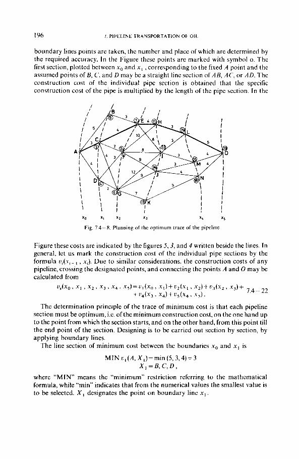
196 7 P l P t 1 INL: ?RANSPORTATION Ot 011
boundary lines points are taken, the number and place of which are determined by the required accuracy. In the Figure these points are marked with symbol 0. The first section, plotted between xo and x1 ,corresponding to the fixed A point and the assumed points of B, C, and D may be a straight line section of AB, AC, or A D . The construction cost of the individual pipe section is obtained that the specific construction cost of the pipe is multiplied by the length of the pipe section. In the
xo X I x 2 x3 x 4 x5
Fig. 7.4 - 8. Planning of the optimum trace of the pipeline
Figure these costs are indicated by the figures S,S, and 4 written beside the lines. In general, let us mark the construction cost of the individual pipe sections by the formula u , ( x , ~ I , x,). Due to similar considerations, the construction costs of any pipeline, crossing the designated points, and connecting the points A and 0 may be calculated from
7.4 - 22
The determination principle of the trace of minimum cost is that each pipeline section must be optimum, i.e. of the minimum construction cost, on the one hand up to the point from which the section starts, and on the other hand, from this point till the end point of the section. Designing is to be carried out section by section, by applying boundary lines.
~ ~ ~ ~ o , ~ I , ~ 2 ~ ~ 3 ~ ~ 4 ~ ~ s ~ = ~ I ~ ~ ~ r ~ 1 ~ + ~ 2 ~ ~ I ~ ~ 2 ~ + ~ ~ ~ X . Z , . x j ) +
+U,(X, 7 X , ) + b ( X 4 , .xs).
The line section of minimum cost between the boundaries xo and xI is
M I N u I ( A , X I ) = min (5,3,4) = 3
where “MIN” means the “minimum” restriction referring to the mathematical formula, while “min” indicates that from the numerical values the smallest value is to be selected. X I designates the point on boundary line x l .
X I = B, C , D ,
7 4 I V T T H F R M A I 011 TRAN\PORT I97
Theconstruction cost of the first, and second line sections between the boundaries .yo and .y2 will be the minimum, if. between A and X 2 points the traces of minimum cost are determined, and from the values obtained. the smallest is choscn. i.e. MIN c ~ , ~ ( A . X 2 ) , I t is to be calculated as follows:
MIN v , , ~ ( A , E ) = M I N [ ( r , ( A . X , ) + r . z ( X I . E ) J = = m i n ( 5 + 3 . 3 + 4 . 4 + x)=7
,Y I = H . c', n
-L sign was used where between the two actual points. because of prohibitcd arcas pipelines may not be layed.
MIN r ' , , , (A ,F)=MIN [ ( V ~ ( A . X , ) + ~ ~ ( X ~ . F ) ] = = min ( 5 + x. 3 + 2.4 + 3 ) = 5
X I = B, C, D MIN I . ~ , ~ ( A . G ) = [ ( ~ , ( A , X , ) + Z . ~ ( X , , G ) J =
= min ( 5 + K . 3 + 4.4 + 2) = 6 .
The minimum values corresponding to the proper points are encircled. The numerical value of
MIN v , , ~ , ~ ( A , H ) ; - ( A , I ) ; - ( A . J ) and - ( A , K )
may be similarly determined. The minimum is
MIN C , , ~ , ~ ( A , X , ) = M I N L ' ~ , ~ , ~ ( A . H ) = I 1 .
Considering the first four sections
MIN 111.2 .3 .4 (A. X 4 ) = M I N r1 .2 .3 .4(A. 4= 14
Finally, for the total line length we can state
C l . 2 . 3 . 4 . S ( A * O ) = M I N [(1 '1 .2 .3 .4(A1 x 4 ) + r 5 ( x 4 , O ) l = =min(14+5 , 16+4, 18+4)=19
X , = L, M , N .
The minimum construction cost is determined by ACEHLO, the solid line in the Figure, the magnitude of which is 19 units.
It can occur with the trace, determined by the above method, that the pipe length is longer, or/and due to the level differences of the pipelines the demand for specific pumping power is greater than in case of other trace variants ofgreater construction costs. Such acase may occur first of all, ifon the terrain, between the two end points, the level difference is very significant, or terrain spots of very high laying costs are present. Then, in order to achieve the determination of the optimum trace, further considerations, and calculations are needed.
The design method, discussed above, among the prevailing Hungarian conditions, decreases the construction cost of the pipeline, by 1.7 - 7.6 percent as compared to the traditional design method.
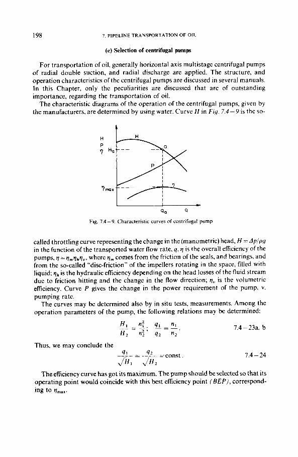
198 7. PIPELINE TRANSPORTATION OF OIL
(e) Selection of centrifugal pumps
For transportation of oil, generally horizontal axis multistage centrifugal pumps of radial double suction, and radial discharge are applied. The structure, and operation characteristics of the centrifugal pumps are discussed in several manuals. In this Chapter, only the peculiarities are discussed that are of outstanding importance, regarding the transportation of oil.
The characteristic diagrams of the operation of the centrifugal pumps, given by the manufacturers, are determined by using water. Curve H in Fig. 7.4 - Y is the so-
t
Fig. 7.4 -9. Characteristic curves of centrifugal pump
called throttling curve representing the change in the (manometric) head, H = A p / p g in the function of the transported water flow rate, q. q is the overall efficiency of the pumps, q = r ] , q h q u , where q , comes from the friction of the seals, and bearings, and from the so-called “disc-friction” of the impellers rotating in the space, filled with liquid; qh is the hydraulic efficiency depending on the head losses of the fluid stream due to friction hitting and the change in the flow direction; qc. is the volumetric efficiency. Curve P gives the change in the power requirement of the pump, v. pumping rate.
The curves may be determined also by in situ tests, measurements. Among the operation parameters of the pump, the following relations may be determined:
Thus, we may conclude the -=- 42 =const JH,JH,
41
7.4-23a, b
7.4 - 24
The efficiency curve has got its maximum. The pump should be selected so that its operating point would coincide with this best efficiency point ( B E P ) , correspond- ing to %lax.
7.4. ISOTHERMAL OIL TRANSPORT 199
By the affinity parabolas, expressing Eq. 7.4-24 in a graphic way, i t can be determined on the one hand the congruent, head curve, at n, speed, of the pump where the original head curve was determined for n, speed, on the other hand, it can be constructed at what speed the given q- H operating point may be realized. On Fig. 7 . 4 - 10, the head curve, represented by solid line is valid for the speed n,. Knowing the B E P (a) determined by q, , and H , , the affinity parabola, intersecting it may be determined, and likewise the affinity parabolas, crossing points hand c may
I
4,24,1 4
Fig. 7 4 - 10.
be also plotted. Points of the head curve, that are valid at the required n, speed may be obtained so, that we read off the intersection point coordinates q a l , H a , belonging to a affinity parabola and speed n, head curve and from the relation, derived from Eq. 7.4 - 23
we calculate the flow rate q,,, whose corresponding affinity parabola point (a') will be, one point of the n, head curve. In the same way, the other points of the new head curve, with the help of the affinity parabolas, may be plotted.
If, however, the n, speed is sought, by which an operating point. defined by the qa2 and H a , values, may be achieved with the maximum possible efficiency, then supposed the coordinates of B E P are known at qal from Eq. 7.4-23 it can be calculated that
9.1
4.2 n,= - n , .
The application ranges of the centrifugal pumps are well shown by the so-called iso-efficiency diagram ( F i g . 7.4 - I I). Beside the head curves, corresponding to different speeds (thicker solid line), some curves, indicating iso-eficiency (thinner solid line) are also shown.
200 7. PIPELINE TRANSPORTATION OF OIL
The brake power, at each q, H, n points of the area, is to be calculated from
7.4 - 25
A frequently accurring problem is that a rate, differring from that of the best efficiency point, generally a smaller rate, must be transported through the pipeline by the pump. Fig. 7.4 - 12 shows the head curve of the pump (H), and the change of H , = h + h, head loss v. rate at the pipeline flow. If, temporarily, a smaller rate than
q Fig. 7.4- 1 1 . Iso-eficiency curves of a centrifugal pump
Fig. 7.4- 12. q’ 9a 9
Determination of the characteristics of the decreased delivery
the above value is to be transported, then two solutions are possible. One of them is, that the gate valve, adjusted after the pump on the pipeline, is throttled to the extent, that the H‘ head, corresponding to the q’ rate should equal the sum of the line head loss, H : , and the h’ throttle loss. It is clear that a significant proportion of the pressure head, developed by the pump, is “uselessly” dissipated in this way. The
1.4. ISOTHERMAL OIL TRANSPORT 20 1
other alternative is that the required rate i s achieved by a decreased pumping speed. lfthe speed is decreased from n, to n,, the operating point 4', H" remains close to the affinity parabola crossing a point. The iso-efficiency curves, represented in Fig. 7.4 - I 1 show that this change is accompanied only by an insignificant decrease in the pump efficiency, and that is why it is generally much more economic than the control by throttling (Fishel and Howe 1979). After Liu (1981), about the energy
A
0 50 100 qlq,, , , ' lo
Fig. 7.4- 13. Energy demand of rate control by throttling(1) and by rpm-alteration (2). after Liu (1981)
requirements of the two control methods information is given by Fig. 7.4- I3 that indicates the specific energy demand P/P,, , , for transportation by throttling (curve I ) , and for transportation by decreased speed (curve 2) in the function of q/qmax. Curve 3 shows the saving, if, instead of the Ihrottling, transportation is accomplished, by change of speed.
I t may occur that a greater rate is to be transported than the capacity of the existing pump. In such cases two, and less frequently more pumps are connected. The connection may be in parallel, or in series. In Fig. 7.4- 14 after Feizlmayr (1975), schemes of pump stations, applying parallel, and serial connections respectively are presented. The pumps of the station in part (a) are in parallel. The station is equipped with safety devices, such as valve and tank, and also with automatic scraper trap. In (b) station the pumps are in series, and here the change of the scraper is also possible. In both cases, the prime mover of the pumps is an asynchronous motor. The regulation of the rate is carried out by throttling.
In most cases the pumps in parallel are alike i.e. they can be characterized individually by the same head curve, transporting oil from a common suction line into a common discharge line. The resultant head curve may be plotted so that the double 4x values of the original head curve are determined at different H, heads. The points, defined in this way, are connected by a solid line (see Fig. 7 .4- 15). The new
202 7. PIPELINE TRANSPORTATION OF OIL
operating point is, thus, determined by the intersection of the system curve, H,. and the resultant head curve (H,,). Accordingly, the corresponding rate will be always smaller than the double value of the rate transported by one pump, i.e. q,l. < 2q,,. In case of crude oil pipelines the parallel connection is considered to be more advantageous, when the static portion of the flow losses is relatively high, i.e. the oil must be transported to “hill”. In the opposite case (e.g.
A I
4 f #.. 0
Y
-D
the dynamic loss is greater),
Sofety volve I Sofely volve II Volve
Control volve
Electric motor
P u m p
sofety t O n k
Scroper l rop Surplus 0 1 1 t O n k
Surplus oil Line Or1 flce Pressure tronsducer Ternperoture fronsducer Level tronsducer s c r o p e r signalling
ChOCk VOlVe
Fig. 7.4- 14. Parallel and series connected oil transport stations, after Feizlmayr (1975)
the serial joining is the more advantageous. Fig. 7.4- f6 shows the original and resultant head curve of the series connected pumps. At any qx point the pressure head H I I x of the resultant curve is of double height, as compared to the original head curve H l x .
The peculiar, series connected first pump of the pump stations is special booster pump. This is generally placed at the deepest point of the area, occupied by tanks, and is a centrifugal pump of big capacity, and small head pressure. Its task is to pump the oil into the suction line of the transporting pump with a pressure, exceeding that of the vapour, and so it may prevent the cavitation damage in the main pump. The booster pump is also able to transport the oil from one tank into the other one, either for treating, or for safety reasons.
The prime movers of the pumps are generally the asynchronous electric motors with fixed, or adjustable speed, operated by alternating current. For the speed
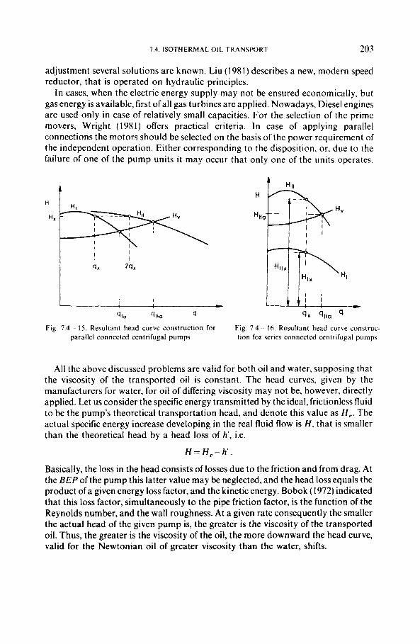
7.4. ISOTHERMAL OIL T R A N S P O R T 203
adjustment several solutions are known. Liu (1981) describes a new, modern speed reductor, that is operated on hydraulic principles.
In cases, when the electric energy supply may not be ensured economically. but gas energy is available, first of all gas turbines are applied. Nowadays, Diesel engines are used only in case of relatively small capacities. For the selection of the prime movers, Wright (1981) offers practical criteria. In case of applying parallel connections the motors should be selected on the basis of the power requirement of the independent operation. Either corresponding to the disposition. or. due to the failure of one of the pump units it may occur that only one of the units operates.
H
Hx
I t
I I 1 1 - 4
qI0 q 110 4 4, 411,
Fig. 7.4- 15. Resultant head curve construction for parallel connected centrifugal pumps
Fig. 7.4- 16. Resultant head curve construc- tion for series connected centrifugal pumps
All the above discussed problems are valid for both oil and water, supposing that the viscosity of the transported oil is constant. The head curves, given by the manufacturers for water, for oil of differing viscosity may not be, however, directly applied. Let us consider the specific energy transmitted by the ideal, frictionless fluid to be the pump’s theoretical transportation head, and denote this value as H e . The actual specific energy increase developing in the real fluid flow is H , that is smaller than the theoretical head by a head loss of h’, i.e.
H = H , - h ’
Basically, the loss in the head consists of losses due to the friction and from drag. At the BEP ofthe pump this latter value may be neglected, and the head loss equals the product of a given energy loss factor, and the kinetic energy. Bobok (1972) indicated that this loss factor, simultaneously to the pipe friction factor, is the function of the Reynolds number, and the wall roughness. At a given rate consequently the smaller the actual head of the given pump is, the greater is the viscosity of the transported oil. Thus, the greater is the viscosity of the oil, the more downward the head curve, valid for the Newtonian oil of greater viscosity than the water, shifts.
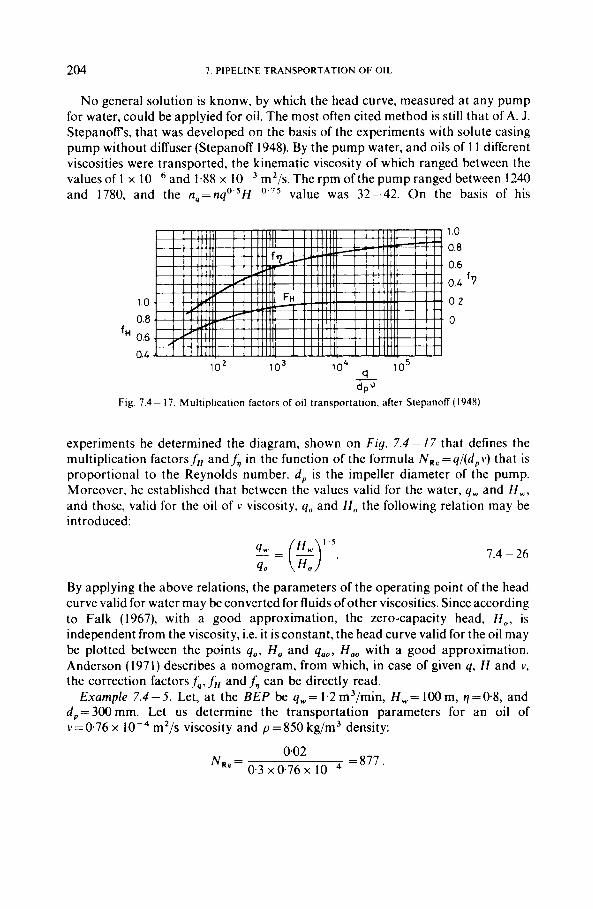
204 7. PIPELINE TRANSPORTATION OF OIL
N o general solution is knonw, by which the head curve, measured at any pump for water, could be applyied for oil. The most often cited method is still that of A. J. StepanofT’s, that was developed on the basis of the experiments with solute casing pump without diffuser (Stepanoff 1948). By the pump water, and oils of 1 1 different viscosities were transported, the kinematic viscosity of which ranged between the valuesof 1 x m2/s.Therpm ofthe pump ranged between 1240 and 1780, and the n,=nqo”H 0 . 7 5 value was 32-42. On the basis of his
and 1.88 x
1.0
0.8 ’’ 0.6 0.4
1 .o 0.8
0.6
0.4 ‘7
0.2
0
lo2 lo3 lo4 cl 1 o5 - * P 3
Fig. 7.4 - 17. Multiplication factors of oil transportation. after Stepanoff (1948)
experiments he determined the diagram, shown on Fig. 7.4 - 17 that defines the multiplication factorsf,, andf, in the function of the formula N R e = q / ( d p v ) that is proportional to the Reynolds number. d, is the impeller diameter of the pump. Moreover, he established that between the values valid for the water, q, and H , , and those, valid for the oil of v viscosity, q, and H , the following relation may be introduced:
7.4 - 26
By applying the above relations, the parameters of the operating point of the head curve valid for water may be converted for fluids of other viscosities. Since according to Falk (1967), with a good approximation, the zero-capacity head, H,, is independent from the viscosity, i.e. i t is constant, the head curve valid for the oil may be plotted between the points q,, H, and q,,, Ha, with a good approximation. Anderson (1971) describes a nomogram, from which, in case of given q, H and v, the correction factorsf,,f, and f , can be directly read.
Example 7.4-5 . Let, at the BEP be q,=1.2m3/min, HW=l00m, q=O.8 , and d,=300mm. Let us determine the transportation parameters for an oil of v=0.76 x m2/s viscosity and p = 8 5 0 kg/m3 density:
=877. 002
R e - 0.3 ~ 0 . 7 6 x N -
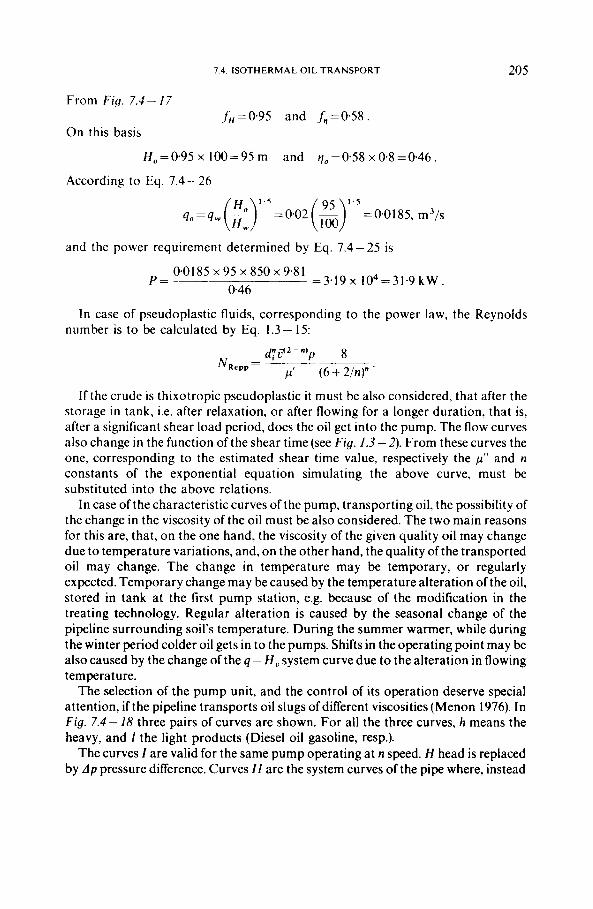
7.4. ISOTHERMAL OIL TRANSPORT 205
From Fig. 7.4 - 17
On this basis fH=095 and f,=0.58
and H , = 0.95 x 100 = 95 m qo = 058 x 0.8 = 0.46
According to Eq. 7.4 - 26
q,, = q., (2)' .' = 0.02 (&) ' ' 5 = 0.01 85, m 3/s
and the power requirement determined by Eq. 7.4 - 25 is
0.01 85 x 95 x 850 x 9.8 1 0.46
p = ~~ = 3 . 1 9 ~ 104=31.9kW.
In case of pseudoplastic fluids, corresponding to the power law, the Reynolds number is to be calculated by Eq. 1.3 - 15:
I f the crude is thixotropic pseudoplastic it must be also considered, that after the storage in tank, i.e. after relaxation, or after flowing for a longer duration, that is, after a significant shear load period, does the oil get into the pump. The flow curves also change in the function of the shear time (see Fig. 1.3 - 2). From these curves the one, corresponding to the estimated shear time value, respectively the p" and n constants of the exponential equation simulating the above curve, must be substituted into the above relations.
In case of the characteristic curves of the pump, transporting oil, the possibility of the change in the viscosity of the oil must be also considered. The two main reasons for this are, that, on the one hand, the viscosity of the given quality oil may change due to temperature variations, and, on the other hand, the quality of the transported oil may change. The change in temperature may be temporary, or regularly expected. Temporary change may be caused by the temperature alteration of the oil, stored in tank at the first pump station, e.g. because of the modification in the treating technology. Regular alteration is caused by the seasonal change of the pipeline surrounding soil's temperature. During the summer warmer, while during the winter period colder oil gets in to the pumps. Shifts in the operating point may be also caused by the change of the q - H , system curve due to the alteration in flowing temperature.
The selection of the pump unit, and the control of its operation deserve special attention, if the pipeline transports oil slugs of different viscosities (Menon 1976). In Fig. 7.4 - 18 three pairs of curves are shown. For all the three curves, h means the heavy, and 1 the light products (Diesel oil gasoline, resp.).
The curves I are valid for the same pump operating at n speed. H head is replaced by A p pressure difference. Curves I ! are the system curves of the pipe where, instead
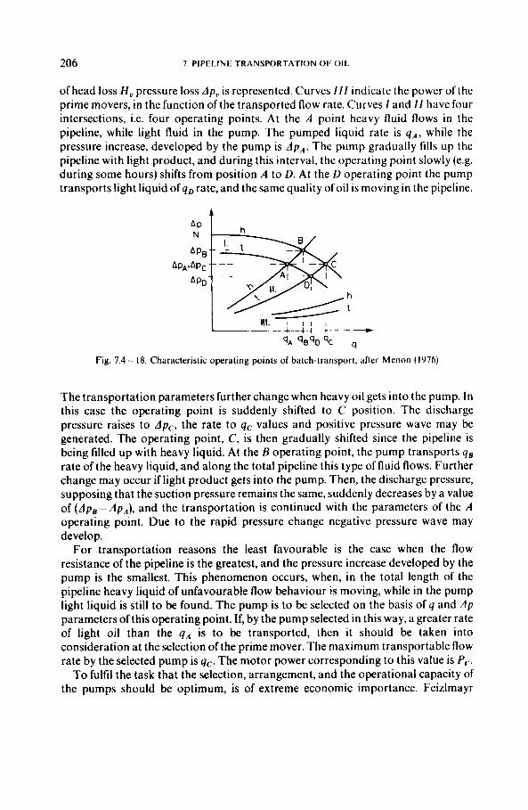
206 7. PIPELINE TRANSPORTATION OF 011
of head loss H, pressure loss Ap, is represented. Curves 111 indicate the power of the prime movers, in the function of the transported flow rate. Curves I and 11 have four intersections, i.e. four operating points. At the A point heavy fluid flows in the pipeline, while light fluid in the pump. The pumped liquid rate is q A , while the pressure increase, developed by the pump is Ap,. The pump gradually fills up the pipeline with light product, and during this interval, the operating point slowly (e.g. during some hours) shifts from position A to D. At the D operating point the pump transports light liquid ofq, rate, and the same quality ofoil is moving in the pipeline.
111. I I I I - qA qBqD qC q
Fig. 7.4- 18. Characteristic operating points of batch-transport, after Menon (1976)
The transportation parameters further change when heavy oil gets into the pump. In this case the operating point is suddenly shifted to C position. The discharge pressure raises to Ap,, the rate to q, values and positive pressure wave may be generated. The operating point, C, is then gradually shifted since the pipeline is being filled up with heavy liquid. At the E operating point, the pump transports 4 s rate of the heavy liquid, and along the total pipeline this type of fluid flows. Further change may occur if light product gets into the pump. Then, the discharge pressure, supposing that the suction pressure remains the same, suddenly decreases by a value of ( L I P , - Ap,), and the transportation is continued with the parameters of the A operating point. Due to the rapid pressure change negative pressure wave may develop.
For transportation reasons the least favourable is the case when the flow resistance of the pipeline is the greatest, and the pressure increase developed by the pump is the smallest. This phenomenon occurs, when, in the total length of the pipeline heavy liquid of unfavourable flow behaviour is moving, while in the pump light liquid is still to be found. The pump is to be selected on the basis of 4 and A p parameters of this operating point. If, by the pump selected in this way, a greater rate of light oil than the q, is to be transported, then it should be taken into consideration at the selection of the prime mover. The maximum transportable flow rate by the selected pump is qc. The motor power corresponding to this value is P,.
To fulfil the task that the selection, arrangement, and the operational capacity of the pumps should be optimum, is of extreme economic importance. Feizlmayr
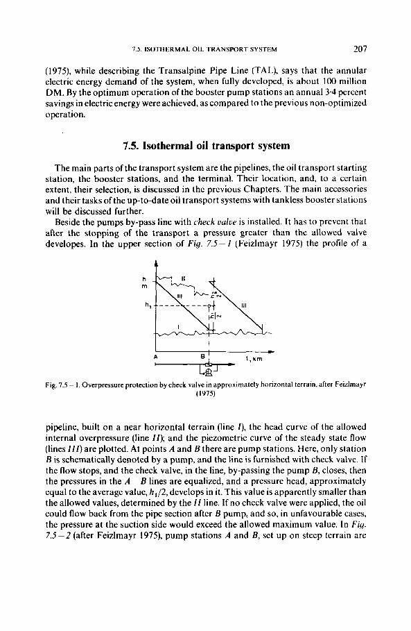
7.5. ISOTHERMAL OIL TRANSPORT SYSTEM 207
(1975), while describing the Transalpine Pipe Line (TAL), says that the annular electric energy demand of the system, when fully developed, is about 100 million DM. By the optimum operation of the booster pump stations an annual 3.4 percent savings in electric energy were achieved, as compared to the previous non-optimized operation.
7.5. Isothermal oil transport system
The main parts of the transport system are the pipelines, the oil transport starting station, the booster stations, and the terminal. Their location, and, to a certain extent, their selection, is discussed in the previous Chapters. The main accessories and their tasks of the up-to-date oil transport systems with tankless booster stations will be discussed further.
Beside the pumps by-pass line with check oaloe is installed. I t has to prevent that after the stopping of the transport a pressure greater than the allowed valve developes. In the upper section of F i g . 7.5-1 (Feizlmayr 1975) the profile of a :b h1 ---- ---+ FIN
I I
A+ ‘Ikrn * Fig. 7.5 - 1. Overpressure protection by check valve in approximately horizontal terrain, after Feizlmayr
(1975)
pipeline, built on a near horizontal terrain (line I), the head curve of the allowed internal overpressure (line I f ) ; and the piezometric curve of the steady state flow (lines I I I ) are plotted. At points A and B there are pump stations. Here, only station B is schematically denoted by a pump, and the line is furnished with check valve. If the flow stops, and the check valve, in the line, by-passing the pump B, closes, then the pressures in the A - B lines are equalized, and a pressure head, approximately equal to the average value, h , / 2 , develops in it. This value is apparently smaller than the allowed values, determined by the I1 line. If no check valve were applied, the oil could flow back from the pipe section after B pump, and so, in unfavourable cases, the pressure at the suction side would exceed the allowed maximum value. In Fig. 7.5-2 (after Feizlmayr 1975), pump stations A and B, set up on steep terrain are
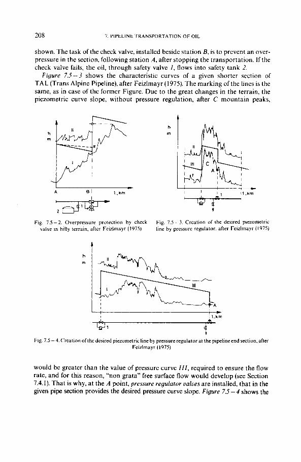
208 7. PIPELINE TRANSPORTATION OF O I L
shown. The task of the check valve, installed beside station B, is to prevent an over- pressure in the section, following station A, after stopping the transportation. If the check valve fails, the oil, through safety valve I, flows into safety tank 2.
Figure 7.5-3 shows the characteristic curves of a given shorter section of TAL (Trans Alpine Pipeline), after Feizlmayr (1975). The marking of the lines is the same, as in case of the former Figure. Due to the great changes in the terrain, the piezometric curve slope, without pressure regulation, after C mountain peaks,
A I , km
*‘**“
Fig. 7.5 - 2. Overpressure protection by check valve in hilly terrain, after Feizlrnayr (1975)
Fig. 7.5 - 3. Creation of the desired piezornetric line by pressure regulator, after Feizlrnayr (1975)
t
1
Fig. 7.5 - 4. Creation of the desired piezornetric line by pressure regulator at the pipeline end section, after Feizlmayr (1975)
would be greater than the value of pressure curve I l l , required to ensure the flow rate, and for this reason, “non grata” free surface flow would develop (see Section 7.4.1). That is why, at the A point, pressure regulator values are installed, that in the given pipe section provides the desired pressure curve slope. Figure 7.5-4 shows the
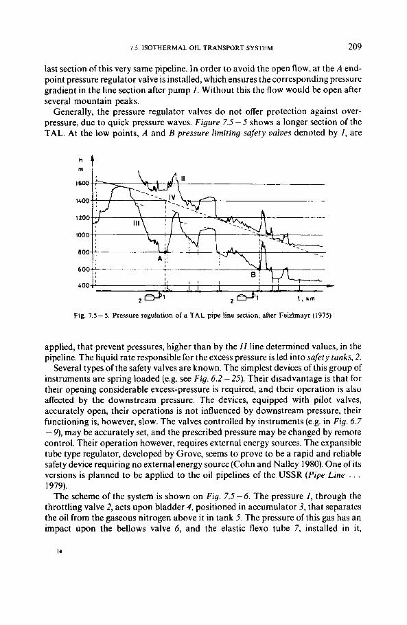
7.5. ISOTHERMAL OIL TRANSPORT SYSTEM 209
last section of this very same pipeline. In order to avoid the open flow, at the A end- point pressure regulator valve is installed, which ensures the corresponding pressure gradient in the line section after pump 1. Without this the flow would be open after several mountain peaks.
Generally, the pressure regulator valves do not offer protection against over- pressure, due to quick pressure waves. Figure 7.5-5 shows a longer section of the TAL. At the low points, A and B pressure limiting safety values denoted by 1, are
h m
1600
1400
1 2 0 0
1000
800
600
4 0 0
Fig. 7.5-5. Pressure regulation of a TAL pipe line section, after Feizlmayr (1975)
applied, that prevent pressures, higher than by the If line determined values, in the pipeline. The liquid rate responsible for the excess pressure is led into safety tanks, 2.
Several types of the safety valves are known. The simplest devices of this group of instruments are spring loaded (e.g. see Fig. 6.2 -25). Their disadvantage is that for their opening considerable excess-pressure is required, and their operation is also affected by the downstream pressure. The devices, equipped with pilot valves, accurately open, their operations is not influenced by downstream pressure, their functioning is, however, slow. The valves controlled by instruments (e.g. in Fig. 6.7 - 9), may be accurately set, and the prescribed pressure may be changed by remote control. Their operation however, requires external energy sources. The expansible tube type regulator, developed by Grove, seems to prove to be a rapid and reliable safety device requiring no external energy source (Cohn and Nalley 1980). One of its versions is planned to be applied to the oil pipelines of the USSR (Pipe Line . . .
The scheme of the system is shown on Fig. 7.5-6. The pressure I , through the throttling valve 2, acts upon bladder 4, positioned in accumulator 3, that separates the oil from the gaseous nitrogen above it in tank 5. The pressure of this gas has an impact upon the bellows valve 6, and the elastic flexo tube 7, installed in it,
1979).
14
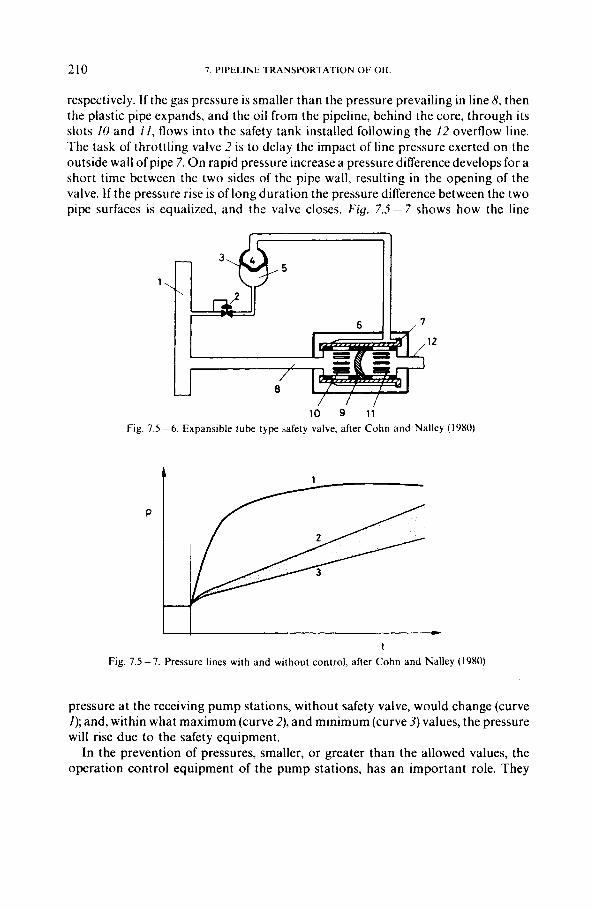
210 7. PIPELINE TRANSPORTATION OF OIL
respectively. If the gas pressure is smaller than the pressure prevailing in line 8, then the plastic pipe expands, and the oil from the pipeline, behind the core, through its slots 10 and 11, flows into the safety tank installed following the f2 overflow line. The task of throttling valve 2 is to delay the impact of line pressure exerted on the outside wall of pipe 7. On rapid pressure increase a pressure difference develops for a short time between the two sides of the pipe wall, resulting in the opening of the valve. If the pressure rise is of long duration the pressure difference between the two pipe surfaces is equalized, and the valve closes. Fig. 7.5-7 shows how the line
1
12
1 0 9 l i
Fig. 7.5 ~ 6. Expansible tube type safety valve, after Cohn and Nalley (1980)
t
Fig. 7.5-7. Pressure lines with and without control, after Cohn and Nalley (1980)
pressure at the receiving pump stations, without safety valve, would change (curve I); and, within what maximum (curve 2), and minimum (curve 3) values, the pressure will rise due to the safety equipment.
In the prevention of pressures, smaller, or greater than the allowed values, the operation control equipment of the pump stations, has an important role. They
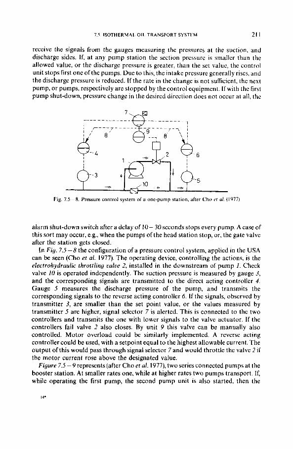
7.5 ISOTHERMAL OIL TRANSPORT SYSTEM 21 1
receive the signals from the gauges measuring the pressures at the suction, and discharge sides. If, at any pump station the section pressure is smaller than the allowed value, or the discharge pressure is greater, than the set value, the control unit stops first one of the pumps. Due to this, the intake pressure generally rises, and the discharge pressure is reduced. I f the rate in the change is not sufficient, the next pump, or pumps, respectively are stopped by the control equipment. I f with the first pump shut-down, pressure change in the desired direction does not occur at all, the
Fig. 7.5 - 8. Pressure control system of a one-pump station, after Cho e / al. (1977)
alarm shut-down switch after a delay of 10- 30 seconds stops every pump. A case of this sort may occur, e.g., when the pumps of the head station stop, or, the gate valve after the station gets closed.
In F i g . 7.5 -8 the configuration of a pressure control system, applied in the USA can be seen (Cho et al. 1977). The operating device, controlling the actions, is the electrohydraulic throttling value 2, installed in the downstream of pump I. Check valve 10 is operated independently. The suction pressure is measured by gauge 3, and the corresponding signals are transmitted to the direct acting controller 4. Gauge 5 measures the discharge pressure of the pump, and transmits the corresponding signals to the reverse acting controller 6 . I f the signals, observed by transmitter 3, are smaller than the set point value, or the values measured by transmitter 5 are higher, signal selector 7 is alerted. This is connected to the two controllers and transmits the one with lower signals to the valve actuator. I f the controllers fail valve 2 also closes. By unit 9 this valve can be manually also controlled. Motor overload could be similarly implemented. A reverse acting controller could be used, with a setpoint equal to the highest allowable current. The output of this would pass through signal selector 7 and would throttle the valve 2 if the motor current rose above the designated value.
Figure 7.5 - 9 represents (after Cho et ul. 1977), two series connected pumps at the booster station. At smaller rates one, while at higher rates two pumps transport. If, while operating the first pump, the second pump unit is also started, then the
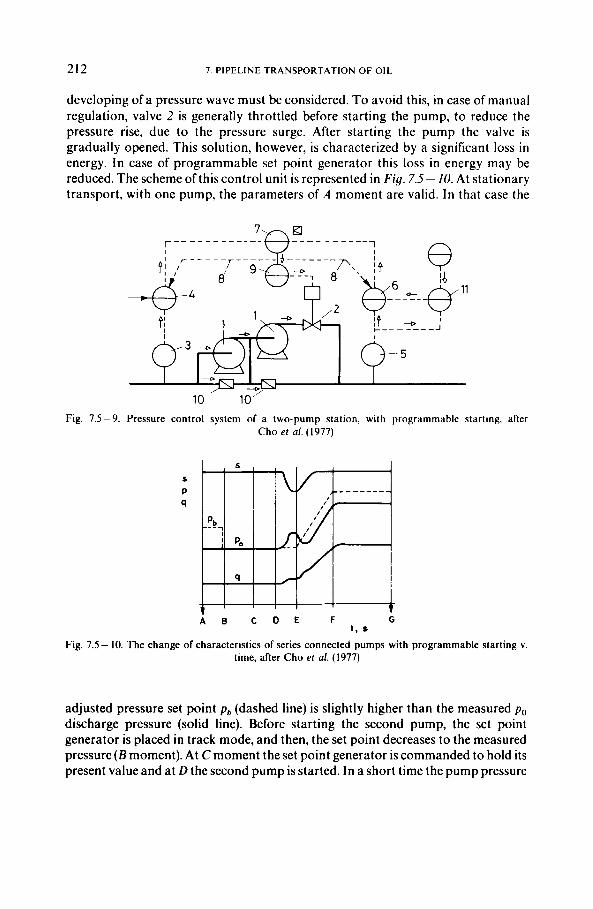
212 7. PIPELINE TRANSPORTATION OF OIL
developing of a pressure wave must be considered. To avoid this, in case of manual regulation, valve 2 is generally throttled before starting the pump, to reduce the pressure rise, due to the pressure surge. After starting the pump the valve is gradually opened. This solution, however, is characterized by a significant loss in energy. In case of programmable set point generator this loss in energy may be reduced. The scheme of thiscontrol unit is represented in Fig. 7.5- 10. At stationary transport, with one pump, the parameters of A moment are valid. In that case the
I r-- - - - - - - - - - -
Fig. 7.5-9. Pressure control system of a two-pump station, with programmable starting, after Cho e? a/ . (1977)
s P q
Fig. 7.5- 10. The change of characteristics of series connected pumps with programmable starting v. time, after Cho er al. (1977)
adjusted pressure set point pa (dashed line) is slightly higher than the measured p o discharge pressure (solid line). Before starting the second pump, the set point generator is placed in track mode, and then, the set point decreases to the measured pressure ( B moment). At C moment the set point generator is commanded to hold its present value and at D the second pump is started. In a short time the pump pressure
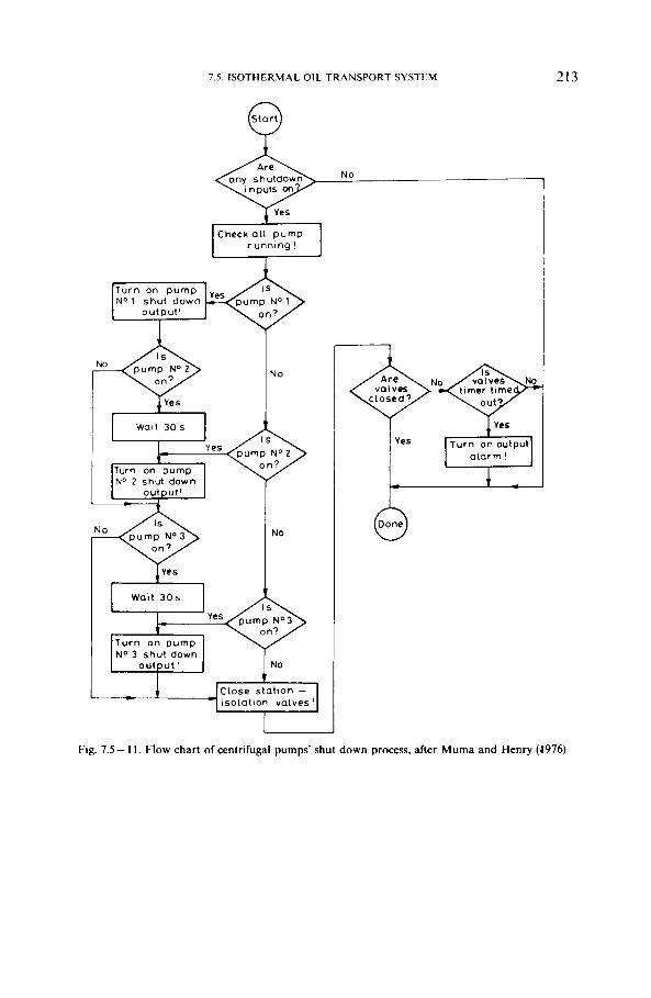
7.5. ISOTHERMAL OIL TRANSPORT SYSTEM
Turn o n pump No 3 shut down
output 1 L
213
Check ol l pump running I
Turn on pump N O 1 shut down Yes pump No 1
output '
W a i t 30s
No 2 shut down output'
1 -
N+ pump NO3 No
valves
Fig. 7.5- 1 1 . Flow chart of centrifugal pumps' shut down process, after Muma and Henry (1976)
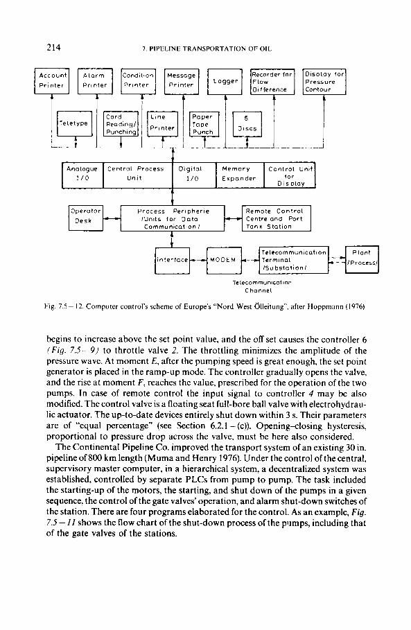
214 7. PIPELINE TRANSPORTATION OF OIL
- Recorder for
Olfference
Account A larm
Printer Prlnter
Teletype
- t
Display fo r Pressure
Line Paper 5 DISCS
Card Reading/ Punching I -Punch
Printer 1 Analogue Central Process
I/O u n i t
Digi tal Memory Control Unlt
I / o E xpander l o r D isp lay
I /
begins to increase above the set point value, and the off set causes the controller 6 (Fig. 7.5-9) to throttle valve 2. The throttling minimizes the amplitude of the pressure wave. At moment E, after the pumping speed is great enough, the set point generator is placed in the ramp-up mode. The controller gradually opens the valve, and the rise at moment F, reaches the value, prescribed for the operation of the two pumps. In case of remote control the input signal to controller 4 may be also modified. The control valve is a floating seat full-bore ball valve with electrohydrau- lic actuator. The up-to-date devices entirely shut down within 3 s. Their parameters are of “equal percentage” (see Section 6.2.1 - (c)). Opening-closing hysteresis, proportional to pressure drop across the valve, must be here also considered.
The Continental Pipeline Co. improved the transport system of an existing 30 in. pipeline of 800 km length (Muma and Henry 1976). Under the control of the central, supervisory master computer, in a hierarchical system, a decentralized system was established, controlled by separate PLCs from pump to pump. The task included the starting-up of the motors, the starting, and shut down of the pumps in a given sequence, the control of the gate valves’ operation, and alarm shut-down switches of the station. There are four programs elaborated for the control. As an example, Fig. 7.5 - I 1 shows the flow chart of the shut-down process of the p’imps, including that of the gate valves of the stations.
Ope ra to r
Desk
Process Peripherie Remote Control /Units f o r Dota - Centre ond Port - Communication I Tank Station
Interface cc M O D E M Telecommunication Plant
lSu bstat ionl IProcessl 4
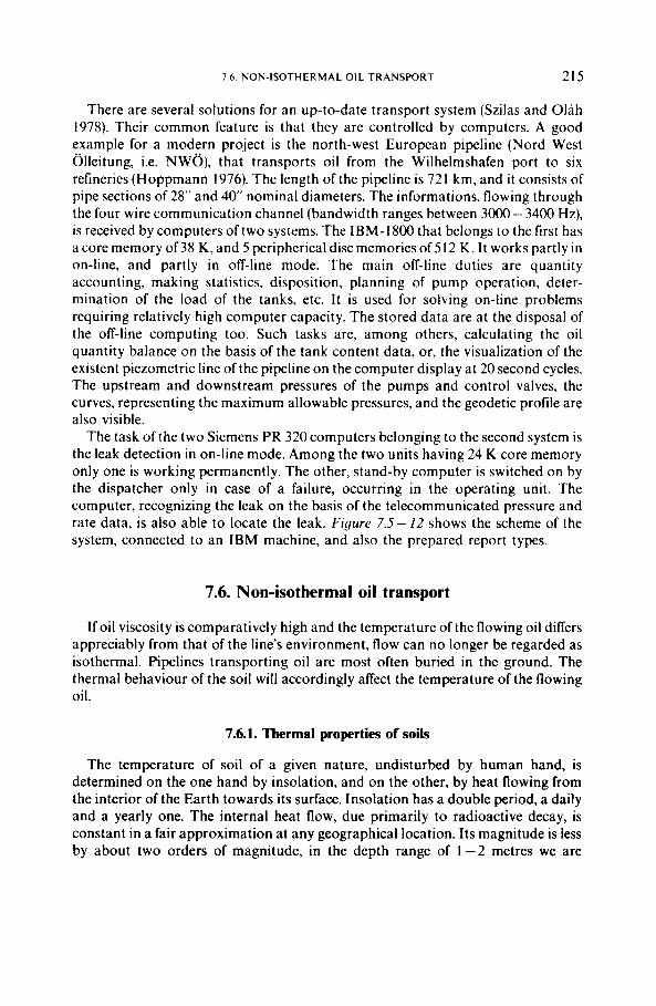
7 6. NON-ISOTHERMAL OIL TRANSPORT 215
There are several solutions for an up-to-date transport system (Szilas and Olih 1978). Their common feature is that they are controlled by computers. A good example for a modern project is the north-west European pipeline (Nord West Olleitung, i.e. NWO), that transports oil from the Wilhelmshafen port to six refineries (Hoppmann 1976). The length of the pipeline is 721 km, and i t consists of pipe sections of 28" and 40' nominal diameters. The informations, flowing through the four wire communication channel (bandwidth ranges between 3000 - 3400 Hz), is received by computers of two systems. The IBM-1800 that belongs to the first has a core memory of 38 K , and 5 peripherical disc memories of 51 2 K. I t works partly in on-line, and partly in off-line mode. The main off-line duties are quantity accounting, making statistics, disposition, planning of pump operation, deter- mination of the load of the tanks, etc. I t is used for solving on-line problems requiring relatively high computer capacity. The stored data are at the disposal of the off-line computing too. Such tasks are, among others, calculating the oil quantity balance on the basis of the tank content data, or, the visualization of the existent piezometric line of the pipeline on the computer display at 20 second cycles. The upstream and downstream pressures of the pumps and control valves, the curves, representing the maximum allowable pressures, and the geodetic profile are also visible.
The task of the two Siemens PR 320 computers belonging to the second system is the leak detection in on-line mode. Among the two units having 24 K core memory only one is working permanently. The other, stand-by computer is switched on by the dispatcher only in case of a failure, occurring in the operating unit. The computer, recognizing the leak on the basis of the telecommunicated pressure and rate data, is also able to locate the leak. Figure 7.5- 12 shows the scheme of the system, connected to an IBM machine, and also the prepared report types.
7.6. Non-isothermal oil transport
If oil viscosity is comparatively high and the temperature of the flowing oil differs appreciably from that of the line's environment, flow can no longer be regarded as isothermal. Pipelines transporting oil are most often buried in the ground. The thermal behaviour of the soil will accordingly affect the temperature of the flowing oil.
7.6.1. Thermal properties of soils
The temperature of soil of a given nature, undisturbed by human hand, is determined on the one hand by insolation, and on the other, by heat flowing from the interior of the Earth towards its surface. Insolation has a double period, a daily and a yearly one. The internal heat flow, due primarily to radioactive decay, is constant in a fair approximation at any geographical location. Its magnitude is less by about two orders of magnitude, in the depth range of 1-2 metres we are
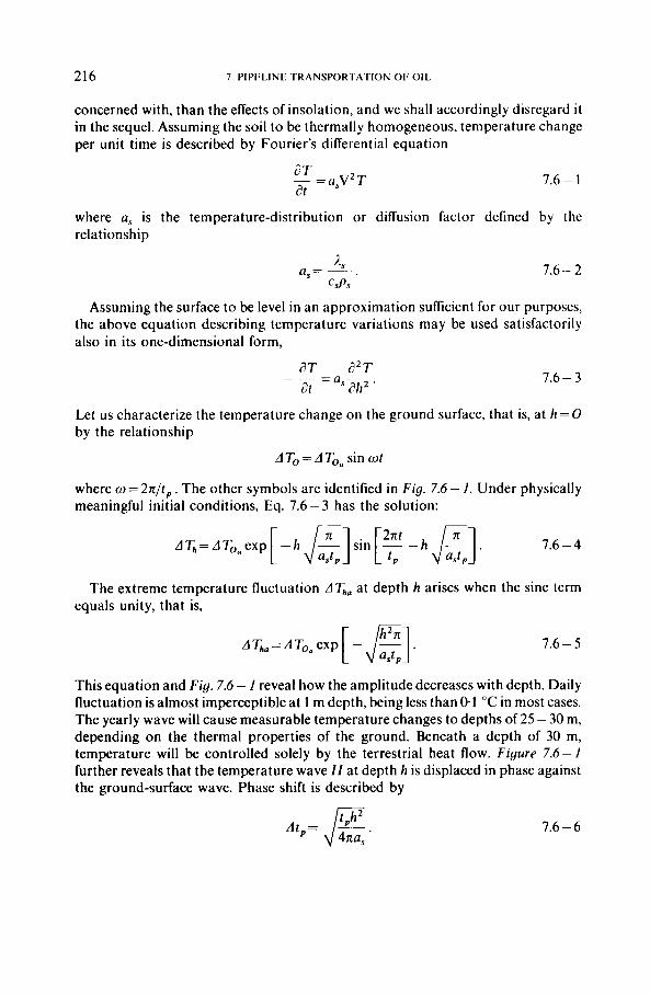
216 7. PIPELINE TRANSPORTATION OF OIL
concerned with, than the effects of insolation, and we shall accordingly disregard i t in the sequel. Assuming the soil to be thermally homogeneous, temperature change per unit time is described by Fourier's differential equation
dT - at =a ,V2T 7.6- 1
where a, is the temperature-distribution or diffusion factor defined by the relationship
7.6 - 2
Assuming the surface to be level in an approximation sufficient for our purposes, the above equation describing temperature variations may be used satisfactorily also in its one-dimensional form,
7.6 - 3
Let us characterize the temperature change on the ground surface, that is, at h = 0 by the relationship
A To = A Ton sin (ot
where w = 2n/tp. The other symbols are identified in Fig. 7.6 - I . Under physically meaningful initial conditions, Eq. 7.6- 3 has the solution:
AT,= AToa exp [ - h F ] sin [F - h p]. a s t p a s t p
7.6 - 4
The extreme temperature fluctuation AT,,, at depth h arises when the sine term equals unity, that is,
7.6 - 5
This equation and Fig. 7.6 - 1 reveal how the amplitude decreases with depth. Daily fluctuation is almost imperceptible at 1 m depth, being less than 0 1 "C in most cases. The yearly wave will cause measurable temperature changes to depths of 25 - 30 m, depending on the thermal properties of the ground. Beneath a depth of 30 m, temperature will be controlled solely by the terrestrial heat flow. Figure 7.6 - I further reveals that the temperature wave I1 at depth h is displaced in phase against the ground-surface wave. Phase shift is described by
7.6 - 6
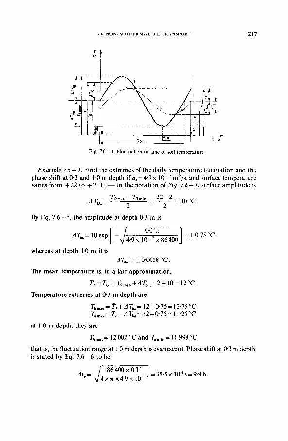
7.6. NON-ISOTHERMAL OIL TRANSPORT 217
Fig. 7.6- 1. Fluctuation in time of soil temperature
Example 7.6- 1. Find the extremes of the daily temperature fluctuation and the phase shift at 0-3 and 1.0 m depth if a,=4.9 x m2/s, and surface temperature varies from + 22 to + 2 "C. - In the notation of Fig. 7.6 - 1, surface amplitude is
By Eq. 7.6-5, the amplitude at depth 0.3 m is
AT,,= lOexp[ 4 9 x -$""--I= x 86400 - +075 "C
whereas at depth 1.0 m it is AT,,= +O.O018 "C.
The mean temperature is, in a fair approximation,
T - T h - o - - Tomi,+dToa=2+ lo= 12 "c. Temperature extremes at 0.3 m depth are
T,,+ ATh= 12+075= 12.75 "C T,min=T'h-AT,,=12-0~75=11~25"C
at 1.0 m depth, they are
Kmax= 12.002 "C and qmin= 11.998 "C
that is, the fluctuation range at 1.0 m depth is evanescent. Phase shift at 0.3 m depth is stated by Eq. 7.6-6 to be
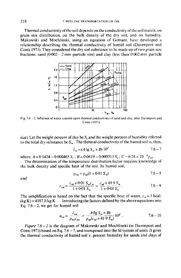
218 7. PIPELINE TRANSPORTATION OF OIL
Thermal conductivity ofthe soil depends on the conductivity of the soil matrix, on grain size distribution, on the bulk density of the dry soil, and on humidity. Makowski and Mochlinski, using an equation of Gemant, have developed a relationship describing the thermal conductivity of humid soil (Davenport and Conti 1971). They considered the dry soil substance to be made up of two grain size fractions: sand (0.002 - 2 mm particle size) and clay (less than 0.002 mm particle
Fig. 7 . 6 -
u
E --. 3
20
16
1.2
0 8
04
0
2. Influence o f water content upon thermal conductivity ofsand and clay, Conti (1971)
after Davenport and
size). Let the weight percent ofclay be S,and the weight percent ofhumidity referred to the total dry substance be S , . The thermal conductivity of the humid soil is, then,
).,=(A IgS,+B) 10' 7.6 - 7
where A=0.1424-0.000465 S,; B=0.0419-0400313 S,; C=6.24 x 10 - 4 ( ) s d .
the bulk density and specific heat of the soil. In humid soil, The determination of the temperature distribution factor requires knowledge of
7.6 - 8
7.6 - 9
The simplification is based on the fact that the specific heat of water, c, = 1 kcal/ (kg K)=4187 J/kg K. - Introducing the factorsdefined by the aboveequations into Eq. 7.6-2, we get for humid soil
7.6- 10
Figure 7.6-2 is the diagram of Makowski and Mochlinski (in Davenport and Conti 1971) based on Eq. 7.6 - 7, and transposed into the SI system of units. I t gives the thermal conductivity of humid soil v. percent humidity for sands and clays of
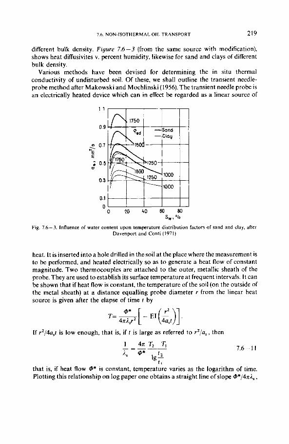
7.6. NON-ISOTHERMAL OIL TRANSPORT 219
different bulk density. Figure 7.6 -3 (from the same source with modification), shows heat diffusivites v. percent humidity, likewise for sand and clays of different bulk density.
Various methods have been devised for determining the in situ thermal conductivity of undisturbed soil. Of these, we shall outline the transient needle- probe method after Makowski and Mochlinski (1956). The transient needle probe is an electrically heated device which can in effect be regarded as a linear source of
1 . 1
0.9
n 0.7 -1 E E
0.5 0
0.3
0.1
0
I I I 1
0 20 40 60 80
Fig. 7.6-3. Influence of water content upon temperature distribution factors of sand and clay, after Davenport and Conti (1971)
S,, "la
heat. It is inserted into a hole drilled in the soil at the place where the measurement is to be performed, and heated electrically so as to generate a heat flow of constant magnitude. Two thermocouples are attached to the outer, metallic sheath of the probe. They are used to establish its surface temperature at frequent intervals. I t can be shown that if heat flow is constant, the temperature of the soil (on the outside of the metal sheath) at a distance equalling probe diameter r from the linear heat source is given after the elapse of time t by
T= -[- @* E I ( L ) ] 4nA,r2 4a,t
If r2/4a,t is low enough, that is, if t is large as referred to r2 /us , then
1 47t T, - T, 7.6 - 1 1
that is, if heat flow @* is constant, temperature varies as the logarithm of time. Plotting this relationship on log paper one obtains a straight line of slope @*/47t1,,
220 7. PIPELINE TRANSPORTATION OF OIL
whence thermal conductivity can be calculated if @* is known. In reality, steady heat flow will take some time to set in and the relationship will become linear after some time only. This time is, however, short enough (of the order of 10s). In pipeline- industry practice, the equation is used in a modified form which takes into account that the thermal properties ofthe probe differ from those ofthe soil, and contains the electric current generating the heat flow - a directly measurable quantity - rather than the heat flow itself. The depth of penetration of the heat flow into the soil is a mere 20- 30 mm, and so the measurement is to be repeated a number of times at any location in order to provide a meaningful mean value.
Thermal conductivity in the undisturbed soil is a function of instantaneous humidity, which is affected by the weather. Accordingly, it is necessary to take soil samples simultaneously with the probe measurements, and to determine on these the humidity of the soil, the bulk density of the dry substance, the clay-to-sand ratio and the specific heat. In the knowledge of these data and using Eqs 7.6-7 and 7.6 - 11, the thermal conductivity and diffusivity of the soil may be extrapolated to any humidity (Davenport and Conti 1971). A longer-term average diffusivity may be determined recording a full temperature wave on the surface and simultaneously at a depth of h m below ground. Both Eqs 7.6 - 5 and 7.6 - 6 are suitable for calculating us in the knowledge of temperature period t , and amplitude ratio AT,, /AT, , and phase shift A t , . - The temperature wave may be recorded over a full year, or over the duration of a shorter ‘harmonic’ wave.
7.6.2. Temperature of oil in steady-state flow, in buried pipelines
The flow temperature of oil injected into a pipeline will usually differ from soil temperature, the soil being mostly cooler than the oil. Assuming the heat flow pattern to be steady-state in and around the pipeline, the variation of axial oil temperature in the pipe can be determined along the pipeline as follows. Part of the potential energy of oil flowing in the pipeline, transformed into heat, will warm the oil. A relative increase in temperature will result also from the solid components’ separating out of the oil. Oil temperature is reduced, on the other hand, by the transfer of heat from the pipeline into the lower-temperature environment.
In calculating the heat generated by friction let us assume the friction gradient along the pipeline to be constant on an average. A pressure-force differential A p d ? n / 4 along a length 1 of pipe generates heat in the amount Q= Apd?nl /4 . Neglecting the reduction in flow rate due to the increasing density of the cooling liquid, we have l = u t and
4
7.6. N O N - I S O T H E R M A L OIL T R A N S P O R T 22 I
Using this relationship we may write up the heat generated by friction per unit of time over unit distance of flow:
Q A P It 1
@*= - = -q[W/m]. 7.6- 12
Let us assume that a temperature drop of 1 "C = 1 K causes the solidification of c kg of solids (to be called paraffin for simplicity) per kg of oil. Let the heat liberated by the solidification of 1 kg of paraffin be K, in which case a temperature drop of 1 "C will liberate heat in the amount of q p x , W/K in a liquid ofgravity p flowing at a rate q per second; t' and K are temperature-dependent, but we shall assume their mcan values to be constant over the temperature range we are concerned with.
Let k denote the heat flow per unit of time into the soil from a unit length of pipe per unit temperature difference, if the whole difference is T, - (where T, is the axial temperature of the oil in the pipeline, and is the original soil temperature at the same depth). k is the heat transfer coefficient per unit length of pipe, which we assume to be constant all along the line. The temperature of flowing oil will decrease by dT, over a length dl. The change in heat content of liquid flowing at the rate 4 under the influence of this temperature difference equals the algebraic sum of the heat generated, on the one hand, and the heat lost to the environment, on the other, over an infinitesimal length of pipe dl, that is,
qpc dT,= @* dl+EqpK dT, - k(T, - T,) dl 7.6- 13
or, in a different formulation,
Let qpc dT, - EqpK dT/= @* dl- kTJ dl -I- kT, dl
q p c - & q p K = A and @ * + k T , = B .
Rearranging and writing up the integration, we have
dT,= d l . B - k T , s
Solving this equation under the initial conditions 1 = 0, T, = TJ1 , and resubstituting the values of A and B, the flow temperature at the end of a pipeline of length 1 turns out to be
T,]-T,-- exp 7.6- 14 @*) k [ -qfl(CktEK)] + ? '
Let us point out that oil temperature will vary also radially in any cross-section of the pipeline. In turbulent flow, radial decrease is slight, but it may be significant in laminar flow. Figure 7.6 - 4 shows one of the possible combinations of flow-velocity and temperature-distribution profiles after Chernikin (1958). Clearly, in this case the axial temperature T, of the oil is somewhat higher than the average temperature.
Example 7.6 - 2. Let the ID of the pipeline be di = 0.2 m, and its length I = 20 km. Oil of gravity p = 8 5 0 kg/m3 flows at a steady rate of q = 100 m3/h through the
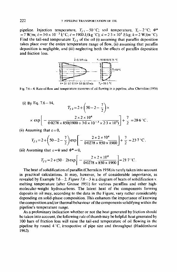
222 7. PIPELINE TRANSPORTATION OF OIL
pipeline. Injection temperature, T, , = 50 "C; soil temperature, = 2 "C; @* = 7 W/m; E= 3.0 x I / T ; C = 1900 J/(kg "C); 2 = 2.3 x 10' J/kg; k = 2 W/(m T). Find the tail-end temperature T,, of the oil (i) assuming that paraffin deposition takes place over the entire temperature range of flow, (ii) assuming that paraffin deposition is negligible, and (iii) neglecting both the effects of paraflin deposition and friction loss.
- V= 0 317m/s T= 55 60 6570 75 ''2
Fig. 7.6 - 4. Rate-of-flow
. - I
V = 01 0 2 03 0 4 05 06 0.7mls
and temperature traverses of oil
Ti- 55 5 O C
flowing in a pipeline, after Chernikin (1958)
(i) By Eq. 7.6- 14, T', = 2 + (50- 2 - i) x
+ ~ = 28.6 "C 1 ' e~p[-0.0278x850(1900+3.0xlo-'x2.3x10~) 2 2 X 2 x 104
(ii) Assuming that E = 0,
+ - =23'7"C. I ' 2 x 2 x 1 0 4 T,, = 2 + (50 - 2 - $) exp [ -
0.0278 x 850 x 1900 2
(iii) Assuming that E = 0 and @* = 0,
=21.7 "C 1 2 x 2 x 1 0 4 [ - 00278 x 850 x 1900 T f 2 = 2 +(50- 2) exp
The heat of solidification of paraffin (Chernikin 1958) is rarely taken into account in practical calculations. It may, however, be of considerable importance, as revealed by Example 7.6- 2. Figure 7.6 -5 is a diagram of heats of solidification v. melting temperature (after Grosse 1951) for various paraffins and other high- molecular-weight hydrocarbons. The latent heat of the components forming deposits in oil may, according to the data in the Figure, vary rather considerably depending on solid-phase composition. This enhances the importance of knowing the composition and/or thermal behaviour of the components solidifying within the pipeline's temperature range.
As a preliminary indication whether or not the heat generated by friction should be taken into account, the following rule of thumb may be helpful: heat generated by 100 bars of friction loss will raise the tail-end temperature of oil flowing in the pipeline by round 4 "C, irrespective of pipe size and throughput (Haddenhorst 1962).
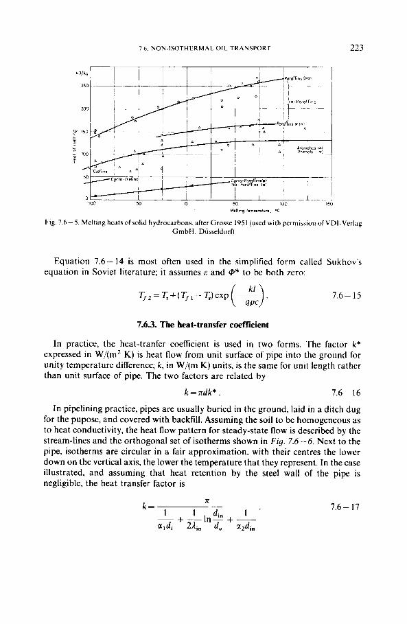
7 6 . N O N - I S O T H E R M A L O I L T R A Y S P O R T
0 - 50 0 50 100 I'
223
H d h g 1.mpmtun. .C
Fig. 7.6- 5. Melting heats ofsolid hydrocarbons. after Grosse 1951 (used with permission of VDI-Verlag GrnbH. DiisseldorQ
Equation 7.6- 14 is most often used in the simplified form called Sukhov's equation in Soviet literature; it assumes E and @* to be both zero:
T,, = T, +( T, , - T,) exp --- ( 3. 7.6- 15
7.6.3. The heat-transfer coefficient
In practice, the heat-tranfer coefficient is used in two forms. The factor k* expressed in W/(m2 K) is heat flow from unit surface of pipe into the ground for unity temperature difference; k, in W/(m K) units, is the same for unit length rather than unit surface of pipe. The two factors are related by
k = ndk* . 7.6- 16
In pipelining practice, pipes are usually buried in the ground, laid in a ditch dug for the pupose, and covered with backfill. Assuming the soil to be homogeneous as to heat conductivity, the heat flow pattern for steady-state flow is described by the stream-lines and the orthogonal set of isotherms shown in F i g . 7.6 -6. Next to the pipe, isotherms are circular in a fair approximation, with their centres the lower down on the vertical axis, the lower the temperature that they represent. In the case illustrated, and assuming that heat retention by the steel wall of the pipe is negligible, the heat transfer factor is
n
1 1 din 1 ~ +--In- + ___ a , d i 2 4 , do azd in
k = 7.6- 17
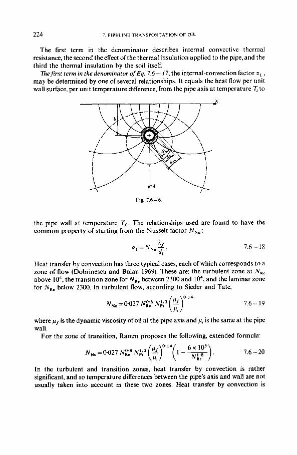
224 7. PIPELINE TRANSPORTATION OF OIL
The first term in the denominator describes internal convective thermal resistance, the second the effect of the thermal insulation applied to the pipe, and the third the thermal insulation by the soil itself.
ntefirst term in the denominator ofEq. 7.6 - 17, the internal-convection factor a, , may be determined by one of several relationships. It equals the heat flow per unit wall surface, per unit temperature difference, from the pipe axis at temperature to
Fig. 7.6-6.
the pipe wall at temperature Tf. The relationships used are found to have the common property of starting from the Nusselt factor NNu :
Jf
di a1 = NN, -. 7.6- 18
Heat transfer by convection has three typical cases, each of which corresponds to a zone of flow (Dobrinescu and Bulau 1969). These are: the turbulent zone at N R e
above lo", the transition zone for N , , between 2300 and lo4, and the laminar zone for N, , below 2300. In turbulent flow, according to Sieder and Tate,
7.6- 19
where p, is the dynamic viscosity of oil at the pipe axis and pi is the same at the pipe wall.
For the zone of transition, Ramm proposes the following, extended formula:
6 x 10' N , , = 0.027 NE;' N;i3 7.6 - 20
In the turbulent and transition zones, heat transfer by convection is rather significant, and so temperature differences between the pipe's axis and wall are not usually taken into account in these two zones. Heat transfer by convection is
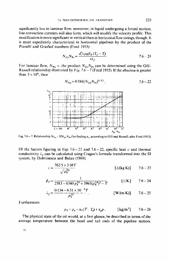
7 6 . NON-ISOTHERMAL. OIL TRANSPORT 225
significantly less in laminar flow; moreover, in liquid undergoing a forced motion. free convection currents will also form, which will modify the velocity profile. This modification is more significant in vertical than in horizontal flow strings, though. I t is most expediently characterized in horizontal pipelines by the product of the Prandtl and Grashof numbers (Ford 1955):
7.6-21
For laminar flow, N , , v. the product N,,N, , can be determined using the Gill- Russell relationship illustrated by F i g . 7.6 - 7 (Ford 1955). If the abscissa is greater than 5 x lo4, then
N , , =0.184(N,,Np1)0~32. 7.6 - 22
"" 10' 8 6 4
2
10
6 4
2
Fig. 7.6- 7. Relationship N , , = f(N,,N,,) for finding z,, according to Gill and Russell; after Ford (1955)
Of the factors figuring in Eqs 7.6-21 and 7.6-22, specific heat c and thermal conductivity 2, can be calculated using Cragoe's formula transformed into the SI system, by Dobrinescu and Bulau ( 1 969):
762.5+3.38T C = Jz
1 " = 2583-- 6340 p:" + 5965(pio)' - T
. 0134-6.31 x lO-'T A/ = -
P i 0
[J/(kg K)] 7.6 - 23
[1/K] 7.6-24
[W/(m K)] 7.6-25
Furthermore
PT=Pn-aT(T-T,)+XpP. [kg/m3 J 7.6 - 26
The physical state of the oil would, at a first glance, be described in terms of the average temperature between the head and tail ends of the pipeline section.
IS
226 7 PIPIlLINE ~I RANSPORTATION 01. OIL
According to Orlicek and Poll (1959, however, heat transfer depends primarily on the nature and state of the liquid film adhering to the pipe wall. The correct procedure would consequently be to determine the physical parameters of the oil at the mean film temperature. No relationship suitable for calculating this temperature has so far been established, however. For practice it seems best to establish parameters for the mean wall temperature of the pipeline section examined. Viscosity depends markedly on temperature, less so on pressure in the range of oil transmission in pipelines. The v=f(p, 7) graphs state results of laboratory measurements. The temperature-dependence of viscosity in Newtonian liquids is best described by Walther's equation
Ig I g ( 1 0 6 v + + ) = b + c I g T
a, b and c are constants depending on the nature of the oil; a ranges from 0.70 to 0.95: putting it equal to 0.8 gives an accuracy sufficient for practical purposes. Hence,
Ig I g ( l O " ~ + 0 ~ 8 ) = b + ~ I g T. 7.6 - 27
This equation implies that oil viscosity v. temperature will be represented by a straight line in an orthogonal system of coordinates whose abscissa (7) axis is logarithmic and whose ordinate (viscosity) axis is doubly logarithmic. This is the Walther-Ubbelohde diagram, whose variant conformable to Hungarian standard MSz-3258-53 is shown as F i g . 7.6-8. In principle, two viscosity values determined at two different temperatures, plotted in this diagram, define a straight line representing the viscosity v. temperature function. In practice, it is indicated to measure viscosity at three temperatures at least, and to use the straight lines joining the three points plotted merely as an aid in interpolating between plots. I t should be ascertained whether or not the oil exhibits anomalous flow behaviour at the lowest temperature of measurement, or evaporation losses at the highest. - Pressure tends to increase viscosity somewhat. According to Dobrinescu and Bulau (l969), dynamic viscosity at pressure p is described by
p,,=p,,(O.9789+0~0261 p:')' O Z p . 7.6 - 28
This relationship gives a 13-percent increase in the viscosity of a 900 kg/m3 density oil between atmospheric pressure and p = 50 bars.
The second term in the denominator ojEq. 7 .6- I 7 is proportional to the thermal resistance of the heat insulation about the pipe; in addition, to the nature of the insulator matrix, the thermal conductivity of the material as i t is dependent primarily on pore volume and pore distribution. I t is primarily the air in the pores that insulates. The thermal conductivity coefficient ofair at room temperature (A,,) is as low as 0.023 W/(m K). If temperature differences between different points of the hole wall make the air in the pores form conduction currents, then heat will flow through the pores by free convection in addition to conduction. The less the mean pore size, the less significant is convection. The resultant thermal conductivity of 'series-connected' small pores and the pore walls separating them is less than it would be for the same overall pore volume if the pores were larger. On the other
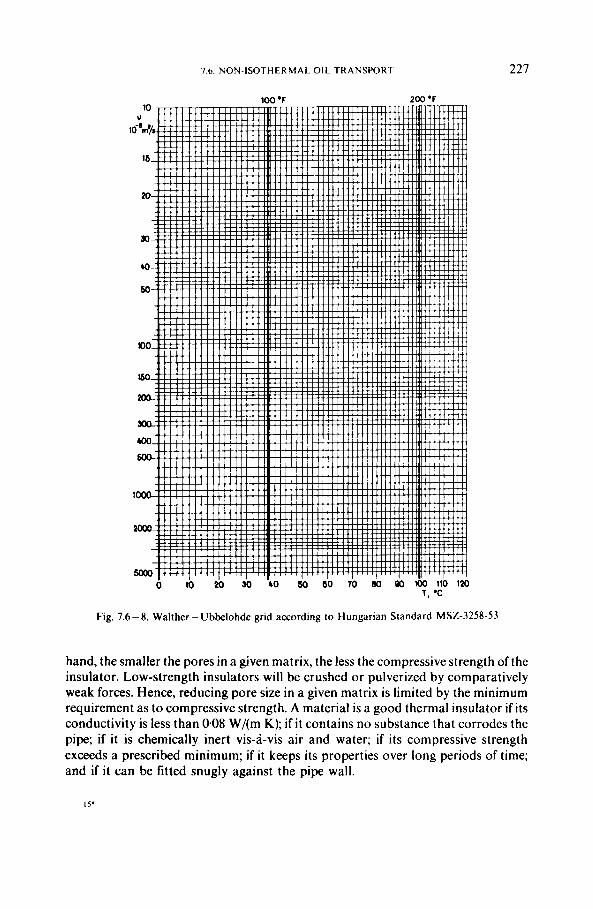
1.6. NON-ISOTHERMAL OIL TRANSPORI 227
Fig. 7.6 - 8. Walther - Ubbelohde grid according to Hungarian Standard MSZ-3258-53
hand, the smaller the pores in a given matrix, the less the compressive strength of the insulator. Low-strength insulators will be crushed or pulverized by comparatively weak forces. Hence, reducing pore size in a given matrix is limited by the minimum requirement as to compressive strength. A material is a good thermal insulator if its conductivity is less than 0.08 W/(m K); if i t contains no substance that corrodes the pipe; if it is chemically inert vis-a-vis air and water; if its compressive strength exceeds a prescribed minimum; if it keeps its properties over long periods of time; and if i t can be fitted snugly against the pipe wall.
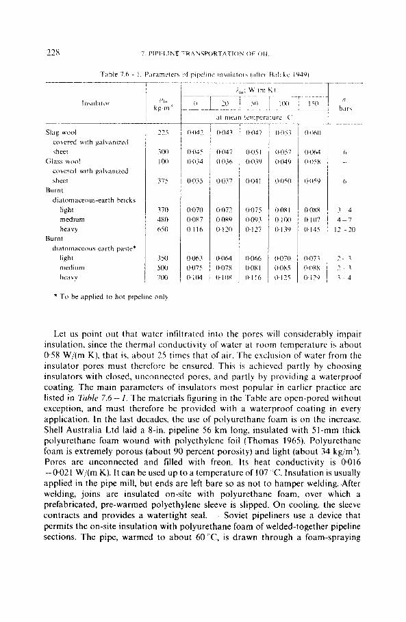
P-C
E -z i:
oz ~ 5 I L-P P- i
Y
9
\Jl’q
U
, 111 iiy “I I
Let us point out that water infiltratcd into the pores will considerably impair insulation, since the thermal conductivity of water at room temperature is about 0.58 W/(m K), that is, about 25 times that of air. The exclusion of water from the insulator pores must thercforc be ensured. This is achieved partly by choosing insulators with closed, unconnected pores, and partly by providing a waterproof coating. The main parameters o f insulators most popular in earlicr practice are listed in Rihle 7.6 - I . The materials figuring in the Table are open-pored without exception, and must therefore be provided with a waterproof coating in every application. In the last decades, the use of polyurethane foam is on the increase. Shell Australia Ltd laid a 8-in. pipeline 56 km long, insulated with 51-mm thick polyurethane foam wound with polyethylene foil (Thomas 1965). Polyurethane foam is extremely porous (about 90 percent porosity) and light (about 34 kg/m'). Pores are unconnected and filled with freon. Its heat conductivity is 0.016 -0.021 W/(m K). I t can be used up to a temperature of 107 "C. Insulation is usually applied in the pipe mill, but ends are left bare so as not to hamper welding..After welding, joins are insulated on-site with polyurethane foam, over which a prefabricated, pre-warmed polyethylene sleeve is slipped. On cooling, the sleeve contracts and provides a watertight seal. - Soviet pipeliners use a device that permits the on-site insulation with polyurethane foam of welded-together pipeline sections. The pipe, warmed to about 6 0 ° C is drawn through a foam-spraying
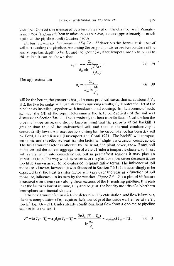
7 h N O N 1\01 H I R M A L 0 1 1 TR4U\ I ’OKT 229
chamber. Correct size is ensured by a tenlpiate fixed on the chamber wall (Zeinalov et ul . 1965). High-grade heat insu!ation is cxpensivc; i t costs approximately as much again 3 s the pipelinc itself (Gautrcr 1970)
11ic ( h i d fc’rm ;17 the dcriomiriutor. (!/‘E4. 7.6 - /7describes the thermal resistrincc o f soil hurrounding the pipeline. Assuming thc original undisturbed tcmperuturc of thc soil at pipcline depth :o bt: ‘<. and the ground-surface tcmpcraturc to be equal t o this value, i t ciin be shown that
7.6 - 79
The approxim ;1 t ‘ Ion
x 2 = 4h di,, In -
d i n
7.6 ~ 30
will be the better, the greater is h/d,, . In most practical cases, that is. at about h/di, 2 2. the two formulae will furnish closely agreeing results; din denotes the O D of thc pipeline as installed. together with insulation and coatings. In the absence of such, d,,=d,,, the O D of the pipe. Determining the heat conductivity of the soil was discussed in Section 7.6.1, ~~~ In determining the hcat transfer factor k valid when the pipeline is operative, one should keep in mind that the porosity of the backfill is greater than that of the undisturbed soil, and that its thermal conductivity is consequently lower. A procedure accounting for this circumstance has been devised by Ford, Ells and Russell (Davenport and Conti 1971). The backfill will compact with time, and the effcctivc heat-transfer factor will slightly increase in consequence. The heat transfer factor is affected by the wind, the plant cover, snow if any, soil moisture and the state of aggregation of water. Under a temperate climate, soil frost will rarely enter into consideration, but in permafrost regions i t may play an important role. The way wind increases k , or the plant or snow cover decrease i t , are too little known as yet to be evaluated in quantitative terms. The influence of soil moisture is known, however ( i t was discussed in Section 7.6.1). I t is accordingly to be expected that the heat transfer factor will vary over the year as a function of soil moisture, influenced in its t u r n by the weather. Figure 7.6 - 9 is a plot of k* factors measured over three years along threc sections of the Friendship pipeline. I t is seen that the factor is lowest in June, Ju ly and August, the hot dry months of a Northern hemisphere continental climate.
I f the heat transfer factor k is to be determined by calculation, and flow is laminar, then the computation of s(, requires the knowledge ofthe inside wall temperature 71, too (cf. Eq. 7.6 - 21). Under steady conditions, heat flow from a one-metre pipeline section into the soil is
27r4,,( T, - T,,)
In ~~
@* = k ( T, - T,) = a,d,n( T, - 7;) = = a2di,,n(7;, - T,) . 7.6-31 d, n
d o
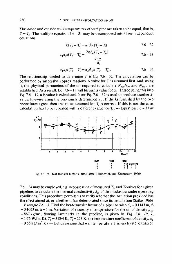
230 7 PIPELINE TRANSPORTATION OF OIL
The inside and outside wall temperatures of steel pipe are taken to be equal, that is, 7;= r,. The multiple equation 7.6- 3 1 may be decomposed into three independent equations:
k ( T, - 7;) = a I din( 7'' - 7;) 7.6 - 32
27&( r, - 7J
din a,d,n(T'- 7;)= ~ ~ ~ _ _ _
1 n, 7.6 - 33
4
sr,d,n(T,- TJ=a,dinrc(Tn- T,) . 7.6 - 34
The relationship needed to determine 7; is Eq. 7.6 - 32. The calculation can be performed by successive approximations. A value for is assumed first, and, using it, the physical parameters of the oil required to calculate N,,N,, and NNu , are established. As a result. Eq. 7.6- 18 will furnish a value for a, . Introducing this into Eq. 7.6 - 17, a k-value is calculated. Now Eq. 7.6 - 32 is used to produce another k- value, likewise using the previously determined a, . If the ks furnished by the two procedures agree, then the value assumed for 7; is correct. If this is not the case, calculation has to be repeated with a different value for r . - Equation 7.6 - 33 or
k' W / m' K
2
1
1 2 3 1, 5 6 7 8 0 l O l l l ? Month
1066 1867 raw 0 8 A pipllw b A A S ; : 0 . C
Fig. 7.6-9. Heat transfer Factor v. time. after Rabinovich and Kuznetsov (1970)
7.6 - 34 may be employed, e.g. in possession of measured Tn and 7; values for a given pipeline, to calculate the thermal conductivity of the insulation under operating conditions. This procedure permits us to verify whether the insulation provided has the effect aimed at, or whether it has deteriorated since its installation (Szilas 1966).
Example 7.6-3. Find the heat-transfer factor of a pipeline with d,=0-1143 m, di =01023 m, h = 1 m. Variation of viscosity v. temperature for the oil of density pzo =887 kg/m3, flowing laminarly in the pipeline, is given in Fig. 7.6-10; A, = 1.76 W/(m K), T,=318.4 K, T,=273 K; the temperature coefficient of density, aT = 0 6 5 kg/(m3 K). - Let us assume that wall temperature is less by 9.5 K than oil
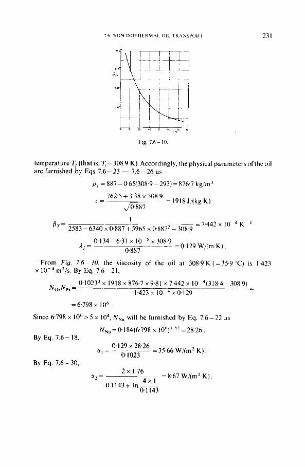
7 6 . NON-ISOTtICRMAI. 011. TKAIUSI'OKI 23 1
Fig. 7.6 - 10.
temperature T,(that is, 7;= 308.9 K). Accordingly, the physical parameters of the oil are furnished by Eqs 7.6 - 23 - 7.6 - 26 as
p T = 887-0.65(308.9-293)=876.7 kg/rn-'
762.5 + 3.38 x 308.9 C = = 1918 J/(kg K ) Jo887
1 = 7 . 4 4 2 ~ 10 K ' IOT = 2583 - 6340 x 0.887 + 5965 x 0887' - 308.9
0.134-6.31 x 10 x 308.9 0.887
=O.I29 W,/(rn K ) )., = ______~~ ~~~ -~
From F i g . 7.6- 10, the viscosity of the oil at 308.9 K ( = 35.9 "C) is 1.423
0.1 0233 x 19 18 x 876.7 x 9.8 1 x 7.442 x 10 4( 3 18.4 - 308.9) 1.423 x lo-" x 0.129
x m2/s. By Eq. 7.6-21,
- - NGrNpr= ~~
= 6.798 x 1 O6 .
Since 6.798 x lo6> 5 x lo4, NN, will be furnished by Eq. 7.6-22 as
NN, =0.184(6.798 x 10')' 3 2 = 28.26. By Eq. 7.6- 18,
0.129 x 28.26 0.1023 a , = = 35.66 W/(m2 K )
By Eq. 7.6 - 30, 2 x 1.76
4 x 1 0.1 143 + In ~
0.1 143
a,= ~ = 8.67 W/(m2 K ) .
232 7. P I P E L I N E T R A N S P O R T A T I O N OF 011.
Now the heat-transfer factor is, by Eq. 7.6- 17,
7L k = = 2.448 W/(m K )
1 1 + - 35.66 x 0. I023 8.67 x 0. I 143
whereas Eq. 7.6 - 32 yields
0.1023 x 7~ x 35'66(318.4-308.9) 318 x 4-273
k = = 2.400 W/(m K ) .
As a further approximation, let 7;=308.7 K , in which case Eq. 7.6-- 17 yields 2.449 W/(m K), and Eq. 7.6 - 32 yields 2.450, so that k = 2.45 W/(m K ) is accepted.
7.6.4. Calculating the head loss for the steady-state flow
(a) The oil is Newtonian
(A) Chernikin's theory
Equation 7.6-2 will hold for an infinitesimal length dl of pipeline only, as the temperature of the oil flowing through the pipe may be considered constant, and so may, in consequence, also ,I and v:
E.llZ
dh - -- d l . * - 2gd,
Equation 1 . 1 - 10 may be used to express 1. also for laminar flow:
7.6 - 35
7.6 - 36
where a and b are constants that, in laminar flow, depend on the flow type only. Substituting this expression of 2 and the expression
7.6 - 37
where the constant coeflicient is
7 h NON-ISOTHERMAL OIL TRANSPORT 233
Viscosity v. temperature in a Newtonian oil may be described over a limited temperature range also by Filonov's explicit formula
,! = y"p - n" 7.6 - 38
where vo is kinematic viscosity at 0 ' C and
where 11, and vI, are experimeritally determined viscosities at the temperatures 7; and 7;, . Let us point out that Tis to be written in "C. vo may be considered as a fictive, extrapolated value. I t has no physical meaning unless the oil is Newtonian al the temperature considered. At a distance 1 from the head end of the pipeline. the temperature of the flowing oil is expressed by Eq. 7.6 - I5 as
where k
4PC
Introducing this into Eq. 7.6-38 , we obtain
m = - ,
Substituting this latter equation in Eq. 7.6-37, we get
7.6 - 39
Let hn( T, , ~ 7J = B, and
then I
h - S A C R ' '"'dl. r - 0
Let Be-"'=u; then, e-"'=u/B. Hence,
1 u I m B mu
I = - - In- and dl= - -du
Substituting the constants into this equation yields R
234 7. PIPELINE TRANSPORTATION OF OIL
Since a,
we have, in the original notation,
x .( Ei [ - hn( T, - T,)] - Ei [ - hn( T, - ' Q e - '"'1 ). . Introducing the v o = v , enTJl implied by Eq. 7.6-38, and the
(T, - T,)e-'"'= T,, - T,
implied by Eq. 7.6- 15, we arrive at
q ( 2 - b ) v b ebn(TJI - T.)
X h l = P - p + ml
x (Ei[ - hn(7'' - T,)] - Eill-hn(Tl, - T,)I) . This equation may be contracted to read
7.6 - 40
7.6-41
in which case, with reference to Eq. 7.6- 37, it may be interpreted as the product of the pressure head loss of a liquid in isothermal flow whose viscosity is v 1 at the head end of the pipeline, of the correction accounting for cooling along the pipeline section A, and of the radial temperature correction A, . In laminar flow, = 128/ng, and b= I ; in turbulent flow, the corresponding values are 0.20l/y and 0.25, if friction factor I is determined using Eq. 1.1 -4 (Chernikin 1958). In Eq. 7.6 -41,
ebn(Tfr - T.4
A , = (Ei[ - bn(T, - T,)] - Ei[ - hn(T12 - T,)]} ml
A, is, then, the correction factor accounting for axial cooling. I t shows how many times the head loss is increased owing to the fact that oil temperature gradually decreases from T, to TJ2 during flow. A, is the correction factor accounting for radial cooling. Its value would be unity if oil temperature were constant over any pipeline cross section. However, temperature in effect decreases from the pipe axis towards the wall (cf. e.g. Example 7.6-4), and hence mean viscosity in the pipe is higher than the axial viscosity. A, accounts for this effect. Chernikin makes use of the Sieder-Tate relationship
0
A , = E (;) 7.6 - 42
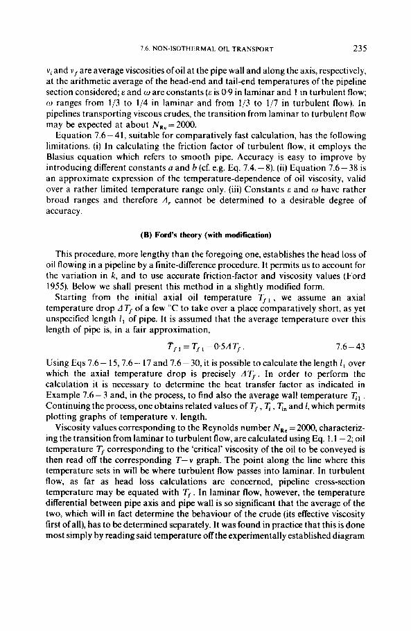
7.6. NON-ISOTHERMAL OIL TRANSPORT 235
viand vf are average viscosities of oil at the pipe wall and along the axis, respectively, at the arithmetic average of the head-end and tail-end temperatures of the pipeline section considered; E and w are constants ( E is 0.9 in laminar and 1 in turbulent flow; o ranges from 1/3 to 1/4 in laminar and from 1/3 to 1/7 in turbulent flow). In pipelines transporting viscous crudes, the transition from laminar to turbulent flow may be expected at about N , , = 2000.
Equation 7.6 - 41, suitable for comparatively fast calculation, has the following limitations. (i) In calculating the friction factor of turbulent flow, it employs the Blasius equation which refers to smooth pipe. Accuracy is easy to improve by introducing different constants a and b (cf. e.g. Eq. 7.4. - 8). (ii) Equation 7.6 - 38 is an approximate expression of the temperature-dependence of oil viscosity, valid over a rather limited temperature range only. (iii) Constants E and w have rather broad ranges and therefore A , cannot be determined to a desirable degree of accuracy.
(B) Ford's theory (with modification)
This procedure, more lengthy than the foregoing one, establishes the head loss of oil flowing in a pipeline by a finite-difference procedure. It permits us to account for the variation in k, and to use accurate friction-factor and viscosity values (Ford 1955). Below we shall present this method in a slightly modified form.
Starting from the initial axial oil temperature T f , , we assume an axial temperature drop ATf of a few "C to take over a place comparatively short, as yet unspecified length I, of pipe. It is assumed that the average temperature over this length of pipe is, in a fair approximation,
T j 1 = Tf I -0'5ATf. 7.6 - 43
Using Eqs 7.6- 15, 7.6- 17 and 7.6- 30, it is possible to calculate the length I , over which the axial temperature drop is precisely ATf. In order to perform the calculation it is necessary to determine the heat transfer factor as indicated in Example 7.6 - 3 and, in the process, to find also the average wall temperature '&., . Continuing the process, one obtains related values of Tf ,7;, Tn and I, which permits plotting graphs of temperature v. length.
Viscosity values corresponding to the Reynolds number N , , = 2000, characteriz- ing the transition from laminar to turbulent flow, are calculated using Eq. 1 . 1 - 2; oil temperature Tf corresponding to the 'critical' viscosity of the oil to be conveyed is then read off the corresponding T-v graph. The point along the line where this temperature sets in will be where turbulent flow passes into laminar. In turbulent flow, as far as head loss calculations are concerned, pipeline cross-section temperature may be equated with Tf . In laminar flow, however, the temperature differential between pipe axis and pipe wall is so significant that the average of the two, which will in fact determine the behaviour of the crude (its effective viscosity first of all), has to be determined separately. It was found in practice that this is done most simply by reading said temperature off the experimentally established diagram
236 7 PIPE1 1NF TRANSPORTATION OF OII
presented as Fig. 7.6 - II, where i t is plotted against the product of thc Grashof and Prandtl numbers. In the knowledge of the diagram i t is possible to establish the variation of corrected oil temperature T f k v. position along the pipc.
By the considerations outlined in Section 1.1, i t is possiblc to find thc dcnsity and friction factor corresponding to the temperatures T, (or 7jk) at the key points of both the turbulent and laminar flow sections along the pipe string. Planinietering
NGr Nf'r
Fig. 7 .6- 1 I . Relationship f o r determining 7,, . after I . o r d (1955)
will furnish the mean values p and relationship
for both zones of flow. Substituting thc
into Eq. 1.1 - I , we obtain the friction loss as
1.6 ~ 44
Introducing the values of and p we obtain the values Ap,.,. and A ~ j 1 , , valid respectively for the turbulent and laminar zone. The full head loss is
4/= &,I + AP,, ' 1.6 ~ 45
The calculation method is shown by the flow chart 7.6 - 12 (Szilas and Navratil 1978, 1981). NRepp equals NR, if the crude exhibits Newtonian flow properties.
Example 7.6-4. Find the friction loss in an uninsulated horizontal pipeline buried in the ground, if di = 102.3 mm; do = 1 14.3 mm; k / d j = 4 x 10 ~ 4; I = 9000 m, TJ,=74"C; T,=O"C;h=l m;i , ,=1~76W/(mK);p, ,=887kg/m' ; ;=50m3/h;r , =0.65 kg/(m3 K), and crude viscosity varies with temperature as shown in Fig. 7.6 - 10. - Let AT,=4 "C; the mean axial temperature T J , of the first pipeline section is, then, 74-4/2=72 "C. Let us find NR, at this temperature. I f i t exceeds 2000, then
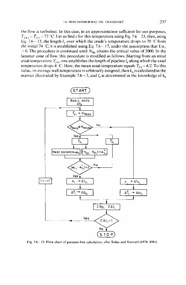
7 h NON-ISOTH1:RMAL O I L T R A N S P O R T 237
Heat bolance-d,,
the flow is turbulent. In this case, in an approximation suflicient for our purposes, 7'; k l = Tf I = 72 "C. Let us find c for this temperature using Eq. 7.6- 23, then, using Eq. !.6- 15, the length I , over which the crude's temperature drops to 70°C from the initial 74 "C; k is established using Eq. 7.6- 17, under the assumption that I / @ , =O. The procedure is continued until N , , attains the critical value of 2000. In the laminar zone of flow, this procedure is modified as follows. Starting from an inital axial temperature 7;,, , one establishes the length of pipeline I,, along which the axial temperaturc drops 4 'C. Here, the mean axial temperature equals Tf,-4/2. To this value, a n average wall temperature is arbitrarily assigned, then k , is calculated in the mannz: illustrated by Example 7.6 - 3, and I , is determined in the knowledge of k ,
(NGr Np,)+a:,
Basic data
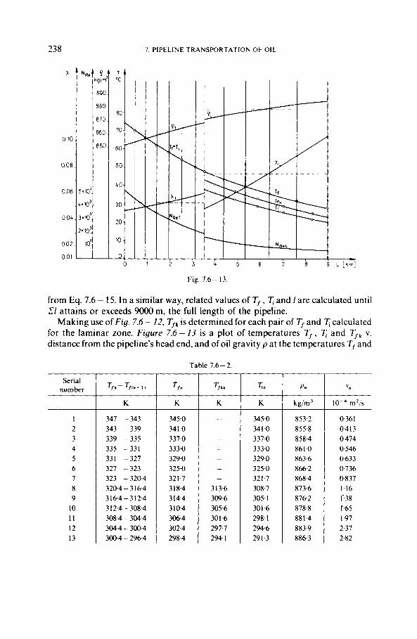
238
a
0 10
0 08
0 06
0 04
002
0 01
-
- -
- -
-
- 3 13.6 309.6 305.6 301.6 297.7 294.1
Fig. 7.6 - I3
345.0 34 1 .O 337.0 333.0 329.0 325.0 321.7 308.7 305.1 301.6 298.1 294.6 291.3
from Eq. 7.6 - 15. In a similar way, related values of 7” , 7; and I are calculated until CI attains or exceeds 9000 m, the full length of the pipeline.
Making use of Fig. 7.6 - 12, T,, is determined for each pair of T, and 7; calculated for the laminar zone. Figure 7.6 - I3 is a plot of temperatures T, , and T,, v. distance from the pipeline’s head end, and of oil gravity pa t the temperatures T, and
Table 7.6 - 2.
Serial number
1 2 3 4 5 6 7 8 9
10 11 12 13
K
347 -343 343 -339 339 -335 335 -331 331 -327 327 -323 323 -320.4 320.4 - 3 16.4 3 16.4 - 3 12.4 3 12.4 - 308.4 308.4 - 304.4 304.4 - 300.4 300.4 - 296.4
T/”
K
345-0 34 1 .O 337.0 333.0 329.0 325.0 321.7 3 18.4 3 14.4 3 10.4 306.4 302.4 298.4
P .
853.2
858.4 855.8
86 I .O 863.6 866.2 868.4 873.6 876.2 878.8
883.9 886.3
881.4
m‘js
0361 0.413 0474 0.546 0.633 0.736 0,837 1.16 1-38 r.65 I .97 2.37 2.82
7.6 NON-ISOTHERMAL OIL TRANSPORT 239
A / ,
rn
450 473 500 529 563 602 420 858 948
1059 1197 1378
23
T,, . The mean density found by planimetering is P T = 861.1 kg/m3 in the turbulent section and p L = 879.4 kg/m3 in the laminar section. The N , , and 1. values at the key points, at temperatures T, and T,, , are likewise plotted in Fig. 7.6 - 13. The mean values of ,I have also been planimetered; they are IT = 0.0432 in turbulent and LL =0.0654 in laminar flow.
Friction loss in the turbulent section is
Ap, ,= 1.95 x 10' N/m2
and in the laminar section
Ap,,, = 4.46 x lo6 N/m
The full friction loss is, then,
Z A l ,
m
450 923
1423 1952 2515 3117 3537 4395 5343 6402 7599 8977 9ooo
dp,=6.41 x lo6 N/m2.
- I O6
All the other relevant intermediate results of the calculation are listed in Table 7.6 - 2.
-
(b) The oil is thixotropic-pseudoplastic
If the flow of the pseudoplastic oil through the pipeline is isothermal, the friction pressure drop, can be calculated by the relations, described in Section 1.3.5. If the oil is not only pseudoplastic but thixotropic too, the shape of the flow curves, serving as a basis for the calculation of the pressure-loss, changes with the shearing time (see Fig. 1.3-2). The flowing pressure loss, for this period of time, may be calculated by the isochronal curves (Ritter and Baticky 1967). The time t , , required for the stabilization is generally of a magnitude of 10 minutes. From this. it is obvious, e.g.
4972 4341 3769 3259 2806 2405 2061 1512 1268 1060 883 733 614
00378 00392 00410 04428 04W8 0.0469 00493 0-0423 0.0505 00604 00725 0.0873 01042
-
-
- -
-
-
-
6.866 5.567 4.467 3.545 2.773 2135
-
-
-
- - -
-
35.76 33.52 31.32 29.13 27.00 24.86
3.1 1 3.1 1 3.1 I 3.1 1 3.1 1 3.1 1 3.1 1 2.45 2.42 2.38 2.34 2.30 2.24
JAkg K)
2047 2033 2019 2005 1990 1976 1964 1935 1920 1906 I892 1878 1865
240 7 PIPELINE TRANSPORTATION OF OIL
that if t , = 25 min, and the flow velocity u = 1 m/s, the flow behaviour of the oil may change before covering a distance of 25 .60 . 1 = 1500 m, and then they get stabilized. During this period, the starting value of the apparent viscosity, and so that of the flow gradient, decreases to a stabilized smaller value. For this reason, with a relatively short pipeline, the use of the isochronal flow curves may be justified. If the length is of 10- I 0 0 km magnitude, however, the accuracy of the pressure loss calculation is insignificantly influenced by the fact, that, the flow gradient is higher in the first section of 1 -2 km length than in the following one. That is why, at long- distance pipelines, the pressure loss is calculated using steady-state flow curves. The flow gradient is constant along the pipeline at isothermal flow, similarly to that of Newtonian fluid flow.
At non-isothermal flow, essentially the procedure, described in Section 7.6.4 - (a, b) is used for pressure loss calculation. A slight modification is needed however because, in order to determine the convection factor, a , (Eq. 7.6- 18). the Nusselt coeficient must be determined as a function of the kinematic viscosity (Eq. 7.6 - 21). For pseudoplastic crudes, instead of this the apparent viscosity, valid for the given shear rate should be used.
7.6.5. Temperature of oil in transient flow, in buried pipelines
In the foregoing sections we have assumed the heat flow about the buried pipeline to be steady. This is the case if the pipeline carries a crude of inflow temperature, flow rate and physical parameters constant over a comparatively long span of time. and the temperature of the soil outside the warmed-up envelope about the pipeline is subject to no change. Strictly speaking, this condition is never satisfied. If, however, departure from the steady state is comparatively slight, procedures outlined in Sections 7.6.2 and 7.6.4 remain applicable.
In numerous cases of considerable practical interest, however, deviation from the steady state may be sufficient to make the steady-state relationships unsuited for even an approximate description of the situation. Transient heat-flow situations of this nature will tend to arise primarily in the following cases: (i) when starting up a hot pipeline: the hot oil flowing into the pipeline that, initially, is as cold as the ground, will gradually warm the environment; (ii) flow in the pipeline is stopped and then started again; (iii) flow rates in the pipeline are subject to fluctuations, (iv) the nature and hence the thermal properties of the crude transported are subject to fluctuations. Any meaningful attempt at solving these problems requires the knowledge of the relationships characterizing the processes of warming and cooling. These will permit the calculation of pressures arising on start-up and restarting, and the variation of said pressures with time.
Numerous models and calculation methods have been devised to describe the transient heat-flow and liquid-flow situations and to solve partial problems all subsumed under the above-stated general problems. To mitigate the complications caused by the large number of variables involved, simplifying assumptions have been introduced, and, as a result of these, individual models may rather
7 6 NON-ISOTHERMAL 011. TKANSPORT 24 I
substantially differ from one another. The first attempts at a synthesis have been published, but the development of theories readily applicable in practice has not by far been accomplished as yet. One publication to be given special mention is Tugunov's academic thesis (Tugunov I968), which summarizes 39 papers written on the subject by the author and his co-workers. Similarly interesting synthescs were presented at the Symposium on 'Waxy crudes in relation to pipeline operations' (London, November 1970). Some of the lectures presented were concerned with transient-flow problems (Davenport and Conti 1971). I t seems, however, too early yet to attempt a synthesis of the results achieved so far in the scope of the present book. In the following I propose to present a transient model which describes the temperature changes of flow v. length and time in a pipeline shut down after steady- state flow (Szilas 1968).
It is assumed that (i) the pipeline is embedded in an infinite half-space filled with soil homogeneous as to thermal behaviour, (ii) the temperature of the soil in contact with the pipeline can be described by the Chernikin model (1958) based on the linear-heat-source theory of Carslaw and Jaeger (1947). - The solution referred to has been used by Chernikin to characterize oil temperatures in non-insulated pipelines, neglecting the difference between the thermal behaviour of oil and soil. In the following I shall derive the 'cooling model' for an insulated pipeline. Let us assume that, at a given instant t , oil temperature is constant all over a certain cross- section of the pipeline, including also the steel pipe cross-section; that is, T, = T, , where suffix o refers to the OD.
Heat flowing through the wall of unity-length pipe into the cooler ground over an infinitesimal length of time dr reduces the temperature of oil and steel by d T
where the symbol T' refers to the transient nature of the process. The heat transfer factor is, after the necessary changes to Eq. 7.6- 17:
Let
7.6 - 46
Cooling will affect not only oil temperature T i , but also the outer surface temperature TI, of the insulation. I t is to describe this change that we shall make use of the Carslaw-Jaeger-Chernikin relationship. Let P , be the image of the projection of the linear heat source on a plane perpendicular to it ( F i g . 7 .6 -14) ; then the
16
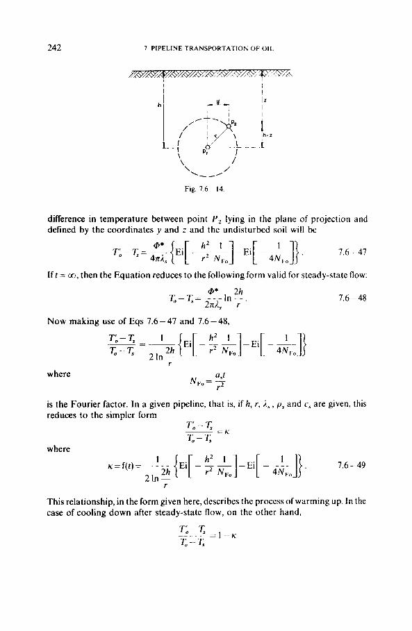
242 7. PIPELINE TRANSPORTATION OF OI[
\ / '- /' Fig. 7.6- 14.
difference in temperature between point P , lying in the plane of projection and defined by the coordinates y and z and the undisturbed soil will be
z-T,= "-{Ei[- - h2 -]-Ei[ 1 - L]}. 7.6-47
4x2, r2 N,, 4Nv0
If t = co, then the Equation reduces to the following form valid for steady-state flow:
@* 2h 2x2, r
To-T,= __ In - . 7.6 - 48
Now making use of Eqs 7.6 - 47 and 7.6 - 48,
where as( N , o = I.'
is the Fourier factor. In a given pipeline, that is, if h, r, i s , p s and c , ~ are given, this reduces to the simpler form
To- T,
T , - K = K
This relationship, in the form given here, describes the process of warming up. In the case of cooling down after steady-state flow, on the other hand,
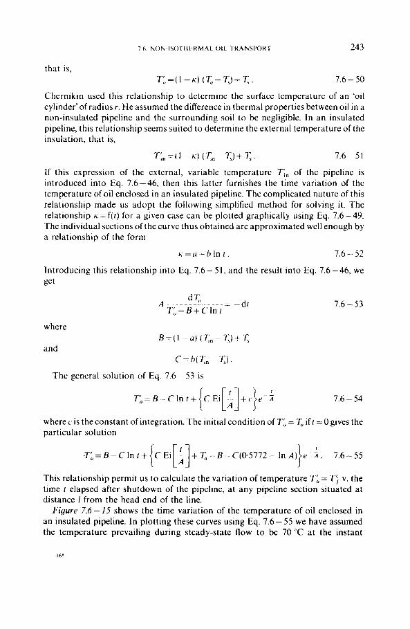
7 6. NON-ISOTHERMAL OIL TRANSPORT 243
that is, Ti,=(I-.) (T,,- TJ+T, 7.6 - 50
Chernikin used this relationship to determine the surface temperature of an 'oil cylinder'of radius r . He assumed the difference in thermal properties between oil in a non-insulated pipeline and the surrounding soil to be negligible. In an insulated pipeline, this relationship seems suited to determine the external temperature of the insulation, that is,
Tr an =( 1 - K ) ( Tn- 7J+ T, . 7.6-51
If this expression of the external, variable temperature TI, of the pipeline is introduced into Eq. 7.6-46, then this latter furnishes the time variation of the temperature of oil enclosed in an insulated pipeline. The complicated nature of this relationship made us adopt the following simplified method for solving it. The relationship ~ = f ( t ) for a given case can be plotted graphically using Eq. 7.6-49. The individual sections of the curve thus obtained are approximated well enough by a relationship of the form
K = u + h I n t . 7.6 - 52
Introducing this relationship into Eq. 7.6- 51, and the result into Eq. 7.6-46, we ge t
= -df 7.6 - 53 d T, T:-B+cG A
where
and
The general solution of Eq. 7.6 - 53 is
T b = B - C I n t + CEi - + c r - 2 i [:I I ' 7.6 - 54
wherecis theconstant ofintegration. The initial condition of To= T,, i f f =Ogives the particular solution
+T,,-B-C(0.5772- I n A ) L' 2. 7.6-55 I ' This relationship permit us to calculate the variation of temperature TI = Tj v. the time f elapsed after shutdown of the pipeline, at any pipeline section situated at distance 1 from the head end of the line.
Figure 7.6 - I5 shows the time variation of the temperature of oil enclosed in an insulated pipeline. In plotting these curves using Eq. 7.6-55 we have assumed the temperature prevailing during steady-state flow to be 70°C at the instant
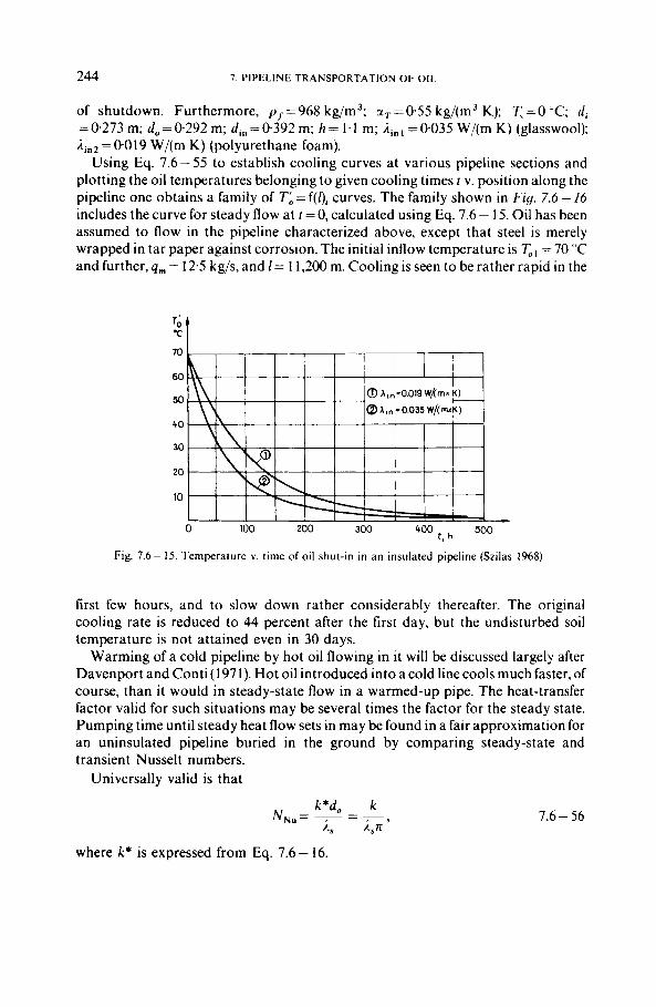
244 7. PIPELINE TRANSPORTATION OF OIL
of shutdown. Furthermore, p r = 968 kg/m3; aT =035 kg/(m3 K); T, = 0 "C; di = 0.273 m; do = 0.292 m; d,, = 0.392 m; h = 1.1 m; iinl = 0.035 W/(m K ) (glasswool); iin2 =0.019 W/(m K ) (polyurethane foam).
Using Eq. 7.6 - 55 to establish cooling curves at various pipeline sections and plotting the oil temperatures belonging to given cooling times i v. position along the pipeline one obtains a family of Tb = f(l), curves. The family shown in Fig. 7.6 - 16 includes the curve for steady flow at t = 0, calculated using Eq. 7.6 - 15. Oil has been assumed to flow in the pipeline characterized above, except that steel is merely wrapped in tar paper against corrosion. The initial inflow temperature is T,, = 70 "C and further, qm = 12.5 kg/s, and 1 = 1 1,200 m. Cooling is seen to be rather rapid in the
500 lroo t , h 0 I00 200 300
Fig. 7.6- 15. Temperature v. time of oil shut-in in an insulated pipeline (Szilas 1968)
first few hours, and to slow down rather considerably thereafter. The original cooling rate is reduced to 44 percent after the first day, but the undisturbed soil temperature is not attained even in 30 days.
Warming of a cold pipeline by hot oil flowing in it will be discussed largely after Davenport and Conti (1971). Hot oil introduced into a cold line cools much faster, of course, than it would in steady-state flow in a warmed-up pipe. The heat-transfer factor valid for such situations may be several times the factor for the steady state. Pumping time until steady heat flow sets in may be found in a fair approximation for an uninsulated pipeline buried in the ground by comparing steady-state and transient Nusselt numbers.
Universally valid is that
7.6 - 56
where k* is expressed from Eq. 7.6- 16.
7.6. NON-ISOTHERMAL. OIL TRANSPORT 245
70
60
50
40
30
20
10
0 0 I 2 3 4 5 6 7 8 8 10 11 12
1, km
Fig. 7.6- 16. Temperature traverses of oil shut-in in a pipeline, at various instants. after shut-in (Szilas 1968)
I f only the heat insulating effect of the soil is considered, then in case of steady- state heat flow, using Eq. 7.6 - 30
2 T i , 4h .
d0
k = a2don = __ 7.6 - 57 In -
Substituting this equation into formula 7.6 - 56 the Nusselt-number valid for steady-state is obtained: -,
For transient heat flow, the following relation is valid:
0.953 N’,,=0.362+ p - j = j ,
FO
where the Fourier number is
7.6 - 58
7.6 - 59
7.6 - 60
If t s is the time required for achieving the steady-state heat flow, then NN, = NL,, and from Eqs 7.6 - 58, 7.6 - 59 and 7.6 - 60 it follows that
r 1 3
7.6-61
246 7. PIPELINE TRANSPORTATION OF OIL
Example 7.6-5. Let us calculate that how much time is required to attain the
Putting the above values into Eq. 7.6-61 we get steady-state heat flow, if do = 0.292 m; h = 1 .1 m; a, = 0.86 x 10 ~ m'/s.
1, =
3
0.953 1 0,292'
= 1.62 Ms = 18.8 days.
In reality, the hypothesis of the infinite half-space will not model the actual heat flow too accurately after the heat flow issuing from the pipeline has attained the ground surface. Heat loss will exceed the calculated value by 10 to 15 percent thereafter. The heat flow pattern will change, however, very slowly, and the time it takes to attain the steady state is infinite in principle. The accuracy of 2, is not as a rule better than 10 percent. Accuracy is not, then, impaired any further if the above relationship is considered to hold also for the steady state.
Flow in pipelines is not usually interrupted long enough for the oil in the pipe to cool down to the undisturbed soil temperature. On restarting. then, the initial temperature is higher than the undisturbed soil temperature, and i t takes less time to attain the steady or a near-steady state. Finding this time for an uninsulated pipeline may be performed by the following consideration. We prepare a family of curves similar to that in F i g . 7.6 -- 16 for the case under consideration. Each curve of the family will be represented in a fair approximation by a 7.6 - 15-type equation. These equations will differ only as to the value of k , but even k will be constant all along a given curve. Putting q p = qm , and c = c, , one may write up for any curve
In AT, - In AT, I 4m"o
k = -- 7.6 - 62
where AT= T- q. Knowing the duration of cooling one may pick out that curve from F i g . 7.6 - 16
which will hold when flow is restarted. I t is necessary to calculate the time i t would take for the oil flowing in the pipe to attain this state if pumping hot oil were started through an entirely cold environment. In order to find it, we use Eq. 7.6-62 to determine the k value corresponding to the actual cooling curve and then Eq. 7.6 - 56 to determine the transient N , , ; Eq. 7.6 - 59 is then used to calculate N , , and Eq. 7.6-60 to find the equivalent pumping time. This is the reduction in the time needed to attain steady heat flow against the case when pumping is started at the undisturbed soil temperature.
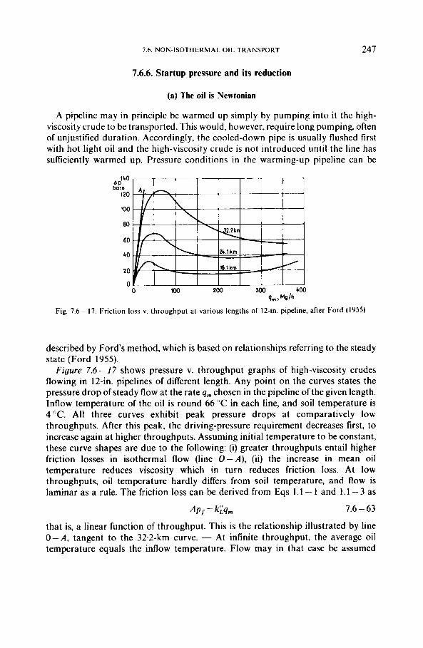
1.6 N O N - I S O T H E R M A L OIL T R A N S P O R T 247
7.6.6. Startup pressure and its reduction
(a) The oil is Newtonian
A pipeline may in principle be warmed up simply by pumping into i t the high- viscosity crude to be transported. This would, however, require long pumping, often of unjustified duration. Accordingly, the cooled-down pipe is usually flushed first with hot light oil and the high-viscosity crude is not introduced until the line has sufficiently warmed up. Pressure conditions in the warming-up pipeline can be
Fig. 7.6- 17. Friction loss v. throughput at various lengths of 12-in. pipeline, after Ford (1955)
described by Ford's method, which is based on relationships referring to the steady state (Ford 1955).
Figure 7.6 - 17 shows pressure v. throughput graphs of high-viscosity crudes flowing in 12-in. pipelines of different length. Any point on the curves states the pressure drop of steady flow at the rate qm chosen in the pipeline of the given length. Inflow temperature of the oil is round 66 "C in each line, and soil temperature is 4 °C . All three curves exhibit peak pressure drops at comparatively low throughputs. After this peak, the driving-pressure requirement decreases first, to increase again at higher throughputs. Assuming initial temperature to be constant, these curve shapes are due to the following: (i) greater throughputs entail higher friction losses in isothermal flow (line 0 - A ) , (ii) the increase in mean oil temperature reduces viscosity which in turn reduces friction loss. At low throughputs, oil temperature hardly differs from soil temperature, and flow is laminar as a rule. The friction loss can be derived from Eqs 1.1 - 1 and 1.1 - 3 as
AP, = k i q m 7.6 - 63
that is, a linear function of throughput. This is the relationship illustrated by line 0 - A , tangent to the 32.2-km curve. - At infinite throughput, the average oil temperature equals the inflow temperature. Flow may in that case be assumed
248 7. PIPELINE TRANSPORTATION OF OIL
turbulent, and on the basis of Eqs 1.1 - 1 and 1 . 1 - 10 we get
Ap,=k'; .q'2-h' 7.6 - 64
where b< 1. The right-hand ends of the curves in Fig. 7.6- 17 approach the line defined by this equation as an asymptote. In plotting any point of these curves we have assumed flow to be steady state. The steady state is not attained instantly, however. Let us assume that a throughput of 100 Mg/h is conveyed through the 24.1-km line. Let us now increase this throughput to I50 Mg/h. At first, the increase in throughput will hardly raise the average temperature of the oil above the preceding steady-state value. Assuming flow to be laminar. a throughput increased by half requires a driving pressure increased by half, that is, pressure drop will suddenly increase from 51 to 76 bars. As time goes on, the average temperature increases gradually, and as a result, A p , decreases to and stabilizes at about 40 bars.
I t follows from the above considerations that pressure drop on startup is invariably higher than that shown in the Figure, the deviation being the higher, the greater the ratio between the throughput to be attained in one step and the steady throughput shown in the Figure. I t is when the step A q is infinitesimal that the values in the Figure prevail. Even in this - unrealistic ~ case it is apparent, however, that startup requires more pressure than steady-state flow. For instance, conveying 350 Mg/h of oil through the 32.2-km line entails a pressure drop of 55 bars, but startup will require a peak pressure of at least 124 bars. If for a delivery pressure of 1 bar the pump can exert 56 bars pressure at most, then this equipment will deliver 14 Mg/h ofoil throughput at most. I t is therefore fundamental that, if the pipeline is to be heated with the oil to be conveyed, the pump must be chosen so as to be able to deliver the peak pressure. In order, furthermore, to make startup fast enough, it is desirable that the pump should exceed said peak by 20- 25 percent at least.
Figure 7.6- I7 further reveals the pressure change to be expected when steady flow is reduced. Let e.g. the steady throughput through the 24.1-km line be 150 Mg/h, and let us reduce this flow to 100 Mg/h. In the first instants of reduction, the temperature of oil flowing in the pipeline will not change; hence, by Eq. 7.6-63, pressure drop will suddenly decrease by one-third, from 40 to round 27 bars. Owing t c the lower flow rate, however, the mean oil temperature will gradually decrease and stabilize at a lower value, while the pressure loss climbs to 54 bars. - Reducing the startup or peak pressure may be achieved by several means. At a point somewhere along the pipeline, a booster or a heater station or both can be installed. Let us assume that the operating conditions characterized by Fig. 7.6 - I7 prevail and that a booster-heater station is installed at the middle ofthe 32.2-km line, that is, at a distance of 16.1 km from both ends. Ifthe intermediate station is used to heat the oil to be conveyed to the inflow temperature of the head end (66 "C), then rhe line may be considered as comprising two 16.1-km segments, whose behaviour is characterized by the lowermost curve in Fig. 7.6 - 17. Peak pressure drop will, then, be 3 1 bars as opposed to the preceding 124 bars. Even if pumping at the intermediate station is avoided, peak pressure will not exceed 2 x 31 =62 bars. Once the line is
7 .6 . NON-ISOTHERMAL OIL TRANSPORT 249
warmed up, heating at the intermediate station may be ceased (and so may pumping, if any). The peak pressure drop to be attained by heating but no pumping at the intermediate station in the 32.2-km line does not significantly exceed the pressure drop of conveying 350 Mg/h of oil in steady flow. If intermediate heating is unfeasible, peak pressure may be reduced by intermediate pumping alone. In the 32.2-km line, this requires a booster pump of round 70 bars pressure. The booster station will, in order to halve the pressure differential, be installed not halfway along the line, but at a distance of about 23 km from the head end.
We have tacitly assumed so far that startup is performed by pumping the same quality crude as is to be conveyed in the steady state. This would, however, often render startup too slow; other, lower-viscosity liquids are used for startup in these cases, such as a light oil or water. Lower viscosity reduces the pressure drop against what is to be expected with the high-viscosity crude; that is, at the maximum allowable operating pressure of the pipe, throughput will be higher and heating will accordingly be faster. If the startup liquid is water, heating is accelerated also because the specific heat ofwater is more than twice that of oil. The drawback of this method is that, on closing down the line, the pipe has to be flushed with the low- viscosity liquid, and the transmission of this latter requires a substantial amount of power. Economy is improved if the water can be put to some use at the tail end, or if the line must at intervals carry light oil anyway.
The startup pressure can be reduced by electric heating of the pipeline cooled down (cf. SECT-system in Section 7.6.7).
(b) The crude is thixotropic-pseudoplastic
Let us create a A p pressure difference between the final cross-sectional areas of gelled crude cylinder being in a horizontal pipe of di diameter and 1 length. Due to this effect, at the inside pipe wall, shear stress 7, arises and the balance of forces may be expressed as follows:
and, hence, the prevailing shear stress at the wall is
di A P ? .= -- - ' 4 I '
7.6 - 65
The relation is also valid for any d diameter value, smaller than di , and thus, by substituting di = 2r, the shear stress on the cylindrical surface of r radius is
7.6 - 66
That is, the shear stress changes linearly v. radius. In the axis of the pipe it equals zero, while at the pipe wall it attains the maximum value expressed by Eq. 7.6 - 65.
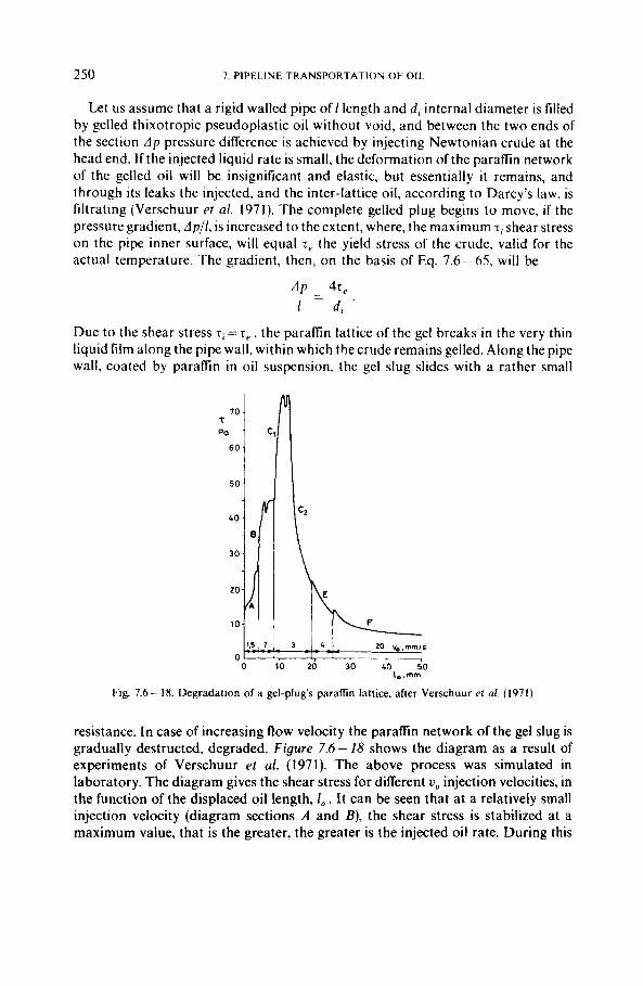
250 7. PIPELINE TRANSPORTATION OF 011
Let us assume that a rigid walled pipe of I length and di internal diameter is filled by gelled thixotropic pseudoplastic oil without void, and between the two ends of the section A p pressure difference is achieved by injecting Newtonian crude at the head end. If the injected liquid rate is small, the deformation of the parafin network of the gelled oil will be insignificant and elastic, but essentially it remains, and through its leaks the injected, and the inter-lattice oil, according to Darcy's law, is filtrating (Verschuur et al. 1971). The complete gelled plug begins to move, if the pressure gradient, A p / l , is increased to the extent, where, the maximum T~ shear stress on the pipe inner surface, will equal T~ the yield stress of the crude, valid for the actual temperature. The gradient, then, on the basis of Eq. 7.6-65, will be
A P 4 T e -
1 di .
Due to the shear stress zi = T, , the paraffin lattice of the gel breaks in the very thin liquid film along the pipe wall, within which the crude remains gelled. Along the pipe wall, coated by paraffin in oil suspension, the gel slug slides with a rather small
70 t
Po
60
50
60
30
20
10
0
I,.mm
Fig. 7.6- 18. Degradation of a gel-plug's paraffin lattice, after Verschuur et al. (1971)
resistance. In case of increasing flow velocity the parafin network of the gel slug is gradually destructed, degraded. Figure 7.6 - 18 shows the diagram as a result of experiments of Verschuur et al. (1971). The above process was simulated in laboratory. The diagram gives the shear stress for different u, injection velocities, in the function of the displaced oil length, I , . It can be seen that at a relatively small injection velocity (diagram sections A and B), the shear stress is stabilized at a maximum value, that is the greater, the greater is the injected oil rate. During this
7 0 NON-ISOTIi1 R M A l 0 1 1 T R A N S P O R l 25 I
period, at the tail and of the experimental pipe, paraflin free oil seeps. C‘, part of the C section is similar to the former. After achieving the maximum shear stress, at the tail end first gelled oil at neariy constant shear stress, then along curve CZ, paraflin in oil suspension at decreasing shear stress flows out. According to curves E: and t.‘, further increase of the injected rate do not significantly influence the ratc of destruction.
The process in pipelines of industrial size, while the oil is cooling and the flow is starting, significantly differs from that describcd above. The main reasons arc:
(i) The compres.sihility of the crude plug in the pipeline. The oil body is compressible for two reasons: on the hand, the crude itself, as a liquid, or gel, is slightly compressible. On the other hand, the gelled crude does not continuously f i l l out the space in the pipeline. The compressibility of the crude, c,, (that is about 7.5 x 10 l o m2/N), and its elasticity constant, E , = l/c,, , respectively may be
determined exactly by laboratory tests. A much more difficult task is, however, the determination of the void fraction volume of the crude in the pipeline. Thc primary reason for its formation is, that, after stopping of the flow, the specific volume of the cooled oil is smaller than that of the warm oil. The void volume will bc relatively significant, if, during the cool-down process, no extra outward liquid “makeup” is injected into the pipeline. Verschuur et al. carried out experiments with a pipeline of 888 m length, and 0.2 m internal diameter. They found, that the void fraction of the
\ ( b )
Fig. 7.6- 19. Pressure wave propagation during gelled oil starting, after Perkins and Turner (1970)
cooled thixotropic pseudoplastic oil could be put to 2 percent, if during the cool- down process the pipe ends were closed. Due to this the compressibility of the oil plug has raised to a 250 times higher value. While calculating the void volume, occurring during the cool-down process, i t should be also considered that during the cooling-down the internal pressure of the pipeline generally decreases, and, also for this reason, the pipe diameter, and its storage volume become smaller. The compressibility factor of the pipe is
di( 1 - v 2 )
s E , ’ c p = ___ 7.6 - 67
252 7. PIPELINE TRANSPORTATION OF OIL
where the pipe wall thickness is s, E , is the elasticity modulus of the pipe material, and v is the Poisson number. The void volume is also decreased by the fact that the specific volume of the crude, due to the pressure drop, slightly increases.
The startup pressure is decreased by the compressibility of the crude and the pipeline. Upon the impact of the “starting oil”, pumped into the pipeline the oil plug does not begin to move along the whole pipe length, and the lattice degradation does not start along the total length, at the same time, but only gradually. First, due to the oil compression, and pipe expansion, a displacement resulting in the partial,
0 5 10 15 20 0-
1 . man
Fig. 7.6- 20. Startup pressure v. time at rigid walled (A) and at elastic pipe line (B), after Perkins and Turner (1970)
or total degradation of the lattice, will develop in the first, I, section of the pipe. The great, initial static shear stress is replaced by a smaller, remanent shear stress. A large portion of the start-up pressure is, thus, preserved for degrading the gel-slug, positioned in next pipeline section I , . Figure 7.6 - 19, after Perkins and Turner (1970) shows, how the pressure wave propagates during the start-up (F ig . a ) , and how great will be the pressure v. length at different t moments calculated from the beginning of the startup ( F i g . b). In Fig. 7.6 -20, after the same above authors, it is shown how the startup pressure v. time changes at a given oil rate, when the pipe is rigid walled (curve A), or when the pipe is elastic (curve B). The startup-pressure reducing effect of the elastic system is visible.
(ii) In the pipeline the cooling effect spreads from outside to inside. This process is assumed to create a laminated structure, parallel to the pipe wall. Little is known about the shape and size of the cavities, and their distribution in the pipe may be rather diversified. In the unmoving parafin network of a given cooling gel section the liquid oil necessarily moves, seeps. If the seepage velocity is rather high, that can be expected first of all in case of rapid cooling, then the space lattice will be more or less destroyed by the flow. Due to this, the yield stress of the gelled oil sections decreases. The factors, influencing this phenomenon, were analyzed among laboratory conditions, by Verschuur e t af. (1971).
(iii) Figure 1.3-4 shows that the yield stress is exponentially increased v. the decrease in the temperature. In the case shown in the Figure, its magnitude increases to a ten times higher value, while the temperature of the oil decreases from 18 “C to
7.6. NON-ISOTHERMAL OIL TRANSPORT 253
8 ’ C. For the reason that the cooling down propagates from outside to inside in the pipeline, the yield stress along the radius decreases t i l l the time, the temperature of the total pipeline content will be equal to that ofthe surrounding soil. That is why, in case of a non-totally cooled-down pipeline, the startup pressure can be equal with a yield stress prevailing in re < ri radius.
(iv) So far it has been tacitly assumed that the paraffin lattice of the gel, filling out the pipe, is of isotropic character before the degradation. Research, carried out quite
0 ‘ - 0 10 20 30 40 50 60 70
t . rnrn
Fig. 7.6- 21. Degradation of the original paraffm lattice (A) and the same procedure, after relaxation ( B ) (Szilas 1981, 1984)
recently, however, has pointed out that the lattice of the cooling oil “remembers” the previous flow, and, in case of formerly laminar flow, the lattice density, perpendicular to the flow direction, may be smaller, than parallel to it (gridshell theory; Szilas 1981, 1984). This latter value can be equal to the yield stress obtained among laboratory conditions. Figure 7.6-21 shows that how the shear stress, at constant shear rate, changes v. time, performing the measurement with rotovisco- meter. Curve A shows the result of the first measurement, while curve B was determined by using the same sample after a relaxation period of 12 hours. It can be seen that the initial shear stress, valid at 0 shear time, and belonging to a given shear rate (injection rate) is smaller in the second case.
254 7 PIPELINE TRANSPORTATION OF OIL
Due to the above listed phenomena the startup pressure of the industrial pipelines may be significantly smaller than the calculated value, based on the yield stress T ~ ,
measured among laboratory conditions and using Eq. 7.6 - 67. So far no relation is known by which for each case, and with a proper accuracy, among the given conditions the startup pressure may be forecasted. By applying Eq. 7.6-67 only the theoretically possible maximum value may be calculated. For industrial design experiments are required among real circumstantes. The qualitative knowledge of the phenomena, however, occurring during the cooling down of the pipeline, can give us a good base to influence the industrial factors for the sake of startup pressure decrease.
I t may be found that the conditions of the cooling down, and restarting is impossible to be controlled to the extent so, that the starting pressure should be low enough. In other words, it may occur that the gelled oil along the total pipe length would not start, in spite of exerting the maximum internal overpressure. In such a case, methods, reducing the startup pressure, are to be employed. Methods of this kind are as follow:
( i ) Due to mixing additives, modifving the p ipe lattice to the oil, not only the flowing gradient is reduced (see Section 7.7.3), but also the static shear stress (yield stress) of the oil. This method, if applyied only for reducing the startup pressure, is rather expensive. since the additive, in case of normal operation, is to be continuously injected. Its great advantage is that i t is totally safe, and the oil treatment accessories requires small space. That is why it is extremely advantageous in case of transporting oil from offshore field’s platforms. This method is used, e.g. at the off shore Bombay High Field, where the oil, treated with additives, is transported to the shore through a pipeline nearly of 200 km length, and 700 mm in diameter.
(ii) The compressibility of the oil significantly increases if gus i s mixed to i t . The startup pressure may be reduced even by only a few percent of gas content. This accounts for the fact, that after the stopping of wells, producing high pour point gassy oils, for the restarting of the flow in the flow line, in certain cases, small startup pressures are needed only.
The disadvantage of this method is, that the presence of the free gas, according to the two-phase flow laws, increases the flow gradient (see Section 1.42). and thus. the specific energy demand of the transport is increased, while the transport capacity of the pipeline is reduced. In certain cases, injection of gas, that due to the oil pressure will dissolve in the oil, may be advantageous. The flow, in case of normal operation, remains of single phase character. After stopping, however, due to the pressure reduction, the gas goes out of the solution, and thus, increases the compressibility of the pipe fluid.
(iii) The startup pressure may be realizable, relatively small, if no temperature drop in the pipeline is allowed, or the cooled-down oil is heuted, respectively. For both purposes the line-heating, described in Section 7.6.7 i s suitable, and for oil pipelines, first of all, it is the SECT system.
(iv) The reduction of the startup pressure of the untreated crude is possible by the sectional startup, that requires proper pipeline accessories. Before establishing
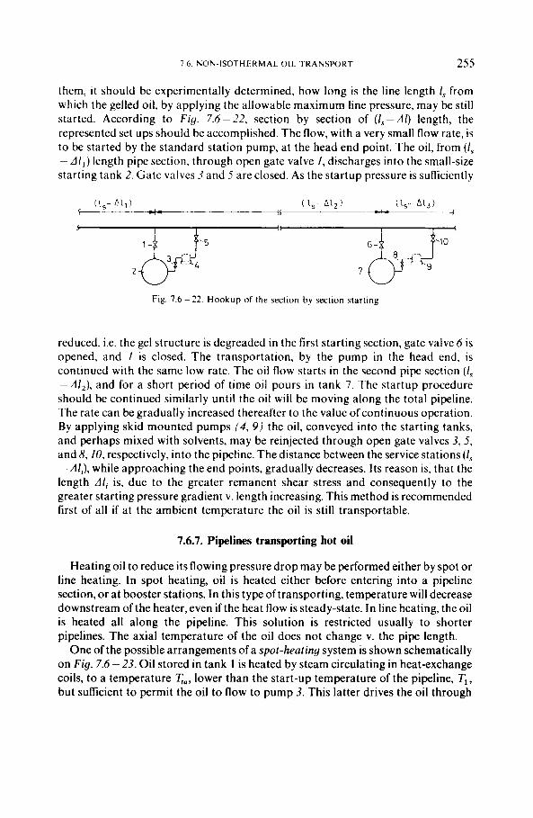
7 6 N O N - I S O T H E R M A L O I L T R A N S P O R T 255
them, i t should be experimentally determined, how long is the line length I , from which the gelled oil, by applying the allowable maximum line pressure, may be still started. According to Fig. 7.6-22, section by section of ( / , - A [ ) length, the represented set ups should be accomplished. The flow, with a very small flow rate, is to be started by the standard station pump, at the head end point. The oil, from ( I , - A l , ) length pipe section, through open gate valve I, discharges into the small-size starting tank 2. Gatc valves 3 and 5 are closed. As the startup pressure is sufficiently
Fig. 7.6-22. Hookup of the section by section starting
reduced, i.e. the gel structure is degreaded in the first starting section, gate valve 6 is opened, and I is closed. The transportation, by the pump in the head end, is continued with the same low rate. The oil flow starts in the second pipe section ( I , - A / 2 ) , and for a short period of time oil pours in tank 7. The startup procedure should be continued similarly until the oil will be moving along the total pipeline. The rate can be gradually increased thereafter to the value of continuous operation. By applying skid mounted pumps (4 , 9) the oil, conveyed into the starting tanks, and perhaps mixed with solvents, may be reinjected through open gate valves 3,5, and 8,10, respectively, into the pipeline. The distance between the service stations ( I , -A! , ) , while approaching the end points, gradually decreases. Its reason is, that the length Al , is, due to the greater remanent shear stress and consequently to the greater starting pressure gradient v. length increasing. This method is recommended first of all if at the ambient temperature the oil is still transportable.
7.6.7. Pipelines transporting hot oil
Heating oil to reduce its flowing pressure drop may be performed either by spot or line heating. In spot heating, oil is heated either before entering into a pipeline section, or at booster stations. In this type of transporting, temperature will decrease downstream of the heater, even if the heat flow is steady-state. In line heating, the oil is heated all along the pipeline. This solution is restricted usually to shorter pipelines. The axial temperature of the oil does not change v. the pipe length.
One of the possible arrangements of a spot -heat ing system is shown schematically on Fig. 7.6 - 23. Oil stored in tank 1 is heated by steam circulating in heat-exchange coils, to a temperature To, lower than the start-up temperature of the pipeline, T,, but sufficient to permit the oil to flow to pump 3. This latter drives the oil through
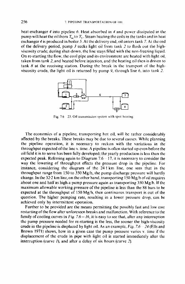
256 7. PIPLI.INE TRANSPORTATION OF 0 1 1
heat-exchanger 4 into pipeline 6. Heat absorbed in 4 and power dissipated in the pump will heat the oil from T,, to T I . Steam heating the coils in the tanks and in heat exchanger 4 is produced in boiler 5. At the delivery end, oil enters tank 7. At the end of the delivery period, pump 3 sucks light oil from tank 2 to flush o u t the high- viscosity crude; during shut-down, the line stays tilled with the non-freezing liquid. O n re-starting the flow, the cool pipe and its environment are heated with light oil, taken from tank 2, and heated before injection, and the heating oil then is driven to tank 8 at the receiving station. During the break in the transport of the high- viscosity crude, the light oil is returned by pump 9, through line 6, into tank 2.
6
Fig. 7.6- 23. Oil transmission system with spot heating
The economics of a pipeline, transporting hot oil, will be rather considerably affected by the breaks. These breaks may be due to several causes. While planning the pipeline operation, it is necessary to reckon with the variations in the throughput expected of the line v. time. A pipeline is often started up even before the oil field it is to serve has been fully developed; the yearly production is less than the expected peak. Referring again to Diagram 7.6 - 17, it is necessary to consider the way the lowering of throughput effects the pressure drop in the pipeline. For instance, considering the diagram of the 24.1 km line, one sees that in the throughput range from 150 to 350 Mg/h, the pump discharge pressure will hardly change. In the 32.2 km line, on the other hand, transporting 150 Mg/h ofoil requires about one and half as high a pump pressure again as transporting 350 Mg/h. If the maximum allowable working pressure of the pipeline is less than the 88 bars to be expected at the throughput of 150 Mg/h, then continuous transport is out of the question. The higher pumping rate, resulting in a lower pressure drop, can be achieved only by intermittent operation.
Further to be provided are the means permitting the possibly fast and low cost restarting of the flow after unforeseen breaks and malfunction. With reference to the family of cooling curves in F i g . 7.6 - 16, i t is easy to see that, after any interruption the pump pressure needed for re-starting is the less, the sooner the high-viscosity crude in the pipeline is displaced by light oil. As an example, F i g . 7.6- 24 (Ells and Brown 1971) shows, how in a given case the pump pressure varies v. time if the displacement of the crude in pipe with light oil is started immediately after the interruption (curve I ) , and after a delay of six hours (curve 2).
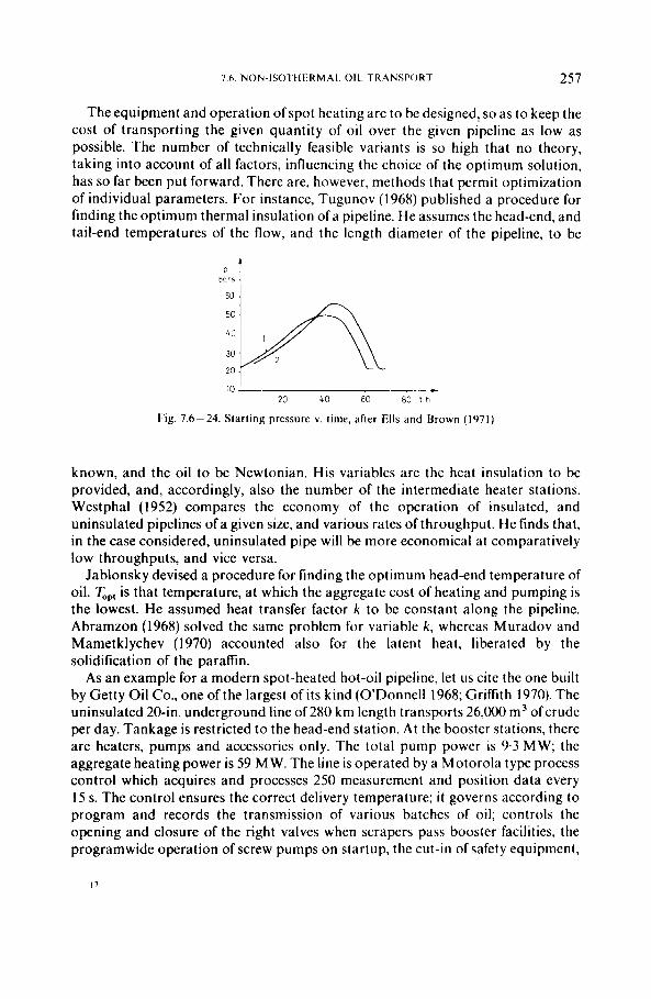
7 h NON-ISOTHERMAI. OIL TRANSPORT 257
The equipment and operation of spot heating are to be designed, so as to keep the cost of transporting the given quantity of oil over the given pipeline as low as possible. The number of technically feasible variants is so high that no theory, taking into account of all factors, influencing the choice of the optimum solution, has so far been put forward. There are, however, methods that permit optimization of individual parameters. For instance, Tugunov (1968) published a procedure for finding the optimum thermal insulation of a pipeline. He assumes the head-end, and tail-end temperatures of the flow, and the length diameter of the pipeline, to be
bars
60
, ----- 20 40 60 80 1 h
10 I
Fig. 7.6-24. Starting pressure v. time, after Ells and Brown (1971)
known, and the oil to be Newtonian. His variables are the heat insulation to be provided, and, accordingly, also the number of the intermediate heater stations. Westphal (1952) compares the economy of the operation of insulated, and uninsulated pipelines of a given size, and various rates of throughput. He finds that, in the case considered, uninsulated pipe will be more economical at comparatively low throughputs, and vice versa.
Jablonsky devised a procedure for finding the optimum head-end temperature of oil. T,,, is that temperature, at which the aggregate cost of heating and pumping is the lowest. He assumed heat transfer factor k to be constant along the pipeline. Abramzon (1968) solved the same problem for variable k , whereas Muradov and Mametklychev (1970) accounted also for the latent heat, liberated by the solidification of the parafin.
As an example for a modern spot-heated hot-oil pipeline, let us cite the one built by Getty Oil Co., one of the largest of its kind (O’Donnell 1968; Grifith 1970). The uninsulated 20-in. underground line of 280 km length transports 26,000 m3 of crude per day. Tankage is restricted to the head-end station. At the booster stations, there are heaters, pumps and accessories only. The total pump power is 9.3 MW; the aggregate heating power is 59 MW. The line is operated by a Motorola type process control which acquires and processes 250 measurement and position data every 15 s. The control ensures the correct delivery temperature; it governs according to program and records the transmission of various batches of oil; controls the opening and closure of the right valves when scrapers pass booster facilities, the programwide operation of screw pumps on startup, the cut-in of safety equipment,
17
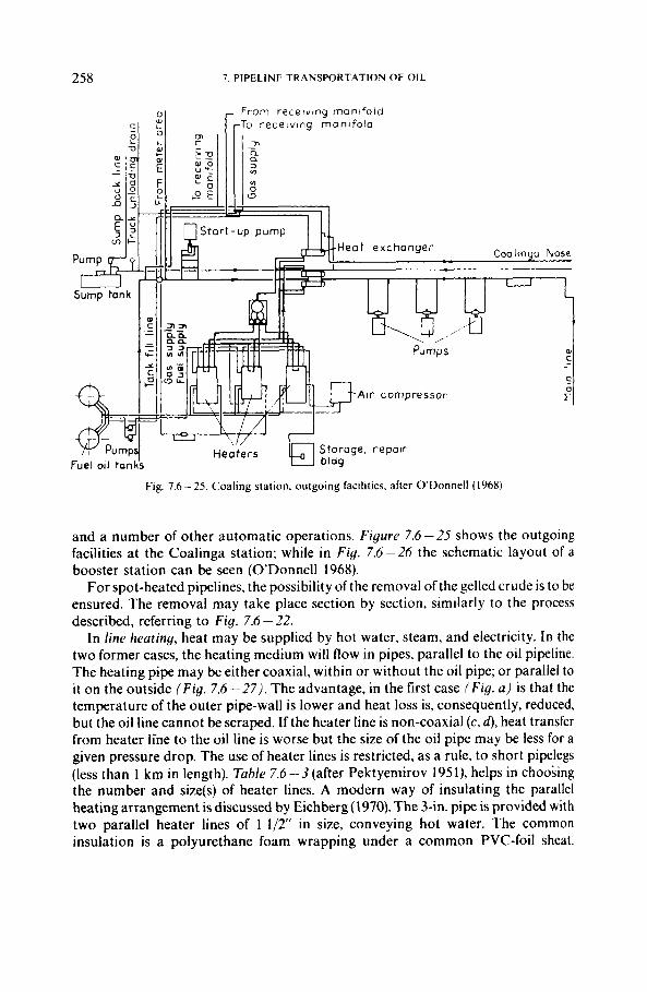
258 7. PIPELINE TRANSPORTATION OF OIL
om r e c e i v i n g manifold r e c e i v i n g rnonifold
Air compressor
Fig. 7.6 - 25. Coaling station, outgoing facilities. after O'Donnell (1968)
and a number of other automatic operations. Figure 7.6-25 shows the outgoing facilities at the Coalinga station; while in Fig. 7.6-26 the schematic layout of a booster station can be seen (ODonnell 1968).
For spot-heated pipelines, the possibility of the removal of the gelled crude is to be ensured. The removal may take place section by section, similarly to the process described, referring to Fig. 7.6 - 22.
In line heating, heat may be supplied by hot water, steam, and electricity. In the two former cases, the heating medium will flow in pipes, parallel to the oil pipeline. The heating pipe may be either coaxial, within or without the oil pipe; or parallel to it on the outside ( F i g . 7.6 -27). The advantage, in the first case ( F i g . a ) is that the temperature of the outer pipe-wall is lower and heat loss is, consequently, reduced, but the oil line cannot be scraped. If the heater line is non-coaxial (c, d), heat transfer from heater line to the oil line is worse but the size of the oil pipe may be less for a given pressure drop. The use of heater lines is restricted, as a rule, to short pipelegs (less than 1 km in length). Table 7.6-3(after Pektyemirov 1951), helps in choosing the number and size(s) of heater lines. A modern way of insulating the parallel heating arrangement is discussed by Eichberg (1970). The 3-in. pipe is provided with two parallel heater lines of 1 1/2" in size, conveying hot water. The common insulation is a polyurethane foam wrapping under a common PVC-foil sheat.
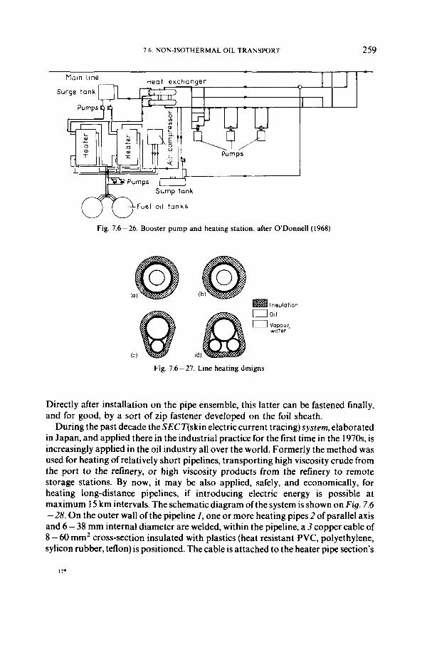
7.6. NON-ISOTHERMAL OIL TRANSPORT 259
Fig. 7.6-26. Booster pump and heating station, after ODonnell (1968)
Fig. 7.6- 27. Line heating designs
Directly after installation on the pipe ensemble, this latter can be fastened finally, and for good, by a sort of zip fastener developed on the foil sheath.
During the past decade the SECT(skin electric current tracing) system, elaborated in Japan, and applied there in the industrial practice for the first time in the 197Os, is increasingly applied in the oil industry all over the world. Formerly the method was used for heating of relatively short pipelines, transporting high viscosity crude from the port to the refinery, or high viscosity products from the refinery to remote storage stations. By now, it may be also applied, safely, and economically, for heating long-distance pipelines, if introducing electric energy is possible at maximum 15 km intervals. The schematic diagram of the system is shown on Fig. 7.6 - 28. On the outer wall of the pipeline I , one or more heating pipes 2 of parallel axis and 6- 38 mm internal diameter are welded, within the pipeline, a 3 copper cable of 8 - 60 mmz cross-section insulated with plastics (heat resistant PVC, polyethylene, sylicon rubber, teflon) is positioned. The cable is attached to the heater pipe section’s
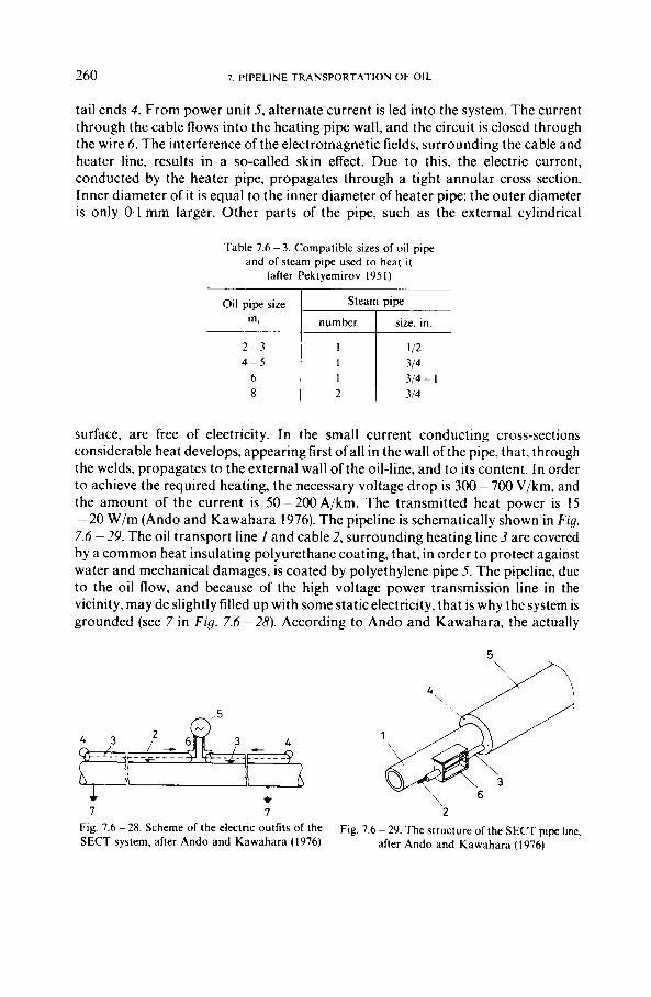
260 7 PIPELINE TRANSPORTATION OF OIL
' I 1
2 1
tail ends 4. From power unit 5, alternate current is led into the system. The current through the cable flows into the heating pipe wall, and the circuit is closed through the wire 6. The interference of the electromagnetic fields, surrounding the cable and heater line, results in a so-called skin effect. Due to this, the electric current, conducted by the heater pipe, propagates through a tight annular cross section. Inner diameter of it is equal to the inner diameter of heater pipe; the outer diameter is only 0.1 mm larger. Other parts of the pipe, such as the external cylindrical
112 3 14
314
314- I
Table 7.6 - 3. Compatible sizes of oil pipe and of steam pipe used to heat i t
(after Pektyemirov 1951)
Oil pipe size in,
2 - 3 4 - 5
6 8
number size, in.
surface, are free of electricity. In the small current conducting cross-sections considerable heat develops, appearing first ofall in the wall ofthe pipe, that, through the welds. propagates to the external wall of the oil-line, and to its content. In order to achieve the required heating, the necessary voltage drop is 300-700 V/km, and the amount of the current is 50-200A/km. The transmitted heat power is 15 - 20 W/m (Ando and Kawahara 1976). The pipeline is schematically shown in Fig. 7.6 -29. The oil transport line I and cable 2, surrounding heating line 3 are covered by a common heat insulating polyurethane coating, that, in order to protect against water and mechanical damages, is coated by polyethylene pipe 5. The pipeline, due to the oil flow, and because of the high voltage power transmission line in the vicinity, may de slightly tilled up with some static electricity, that is why the system is grounded (see 7 in F i g . 7.6 -28). According to Ando and Kawahara, the actually
5
4yj i+&i7L 1
- - - - - - - - - - - - _ - _ _ _ - _
7 7 2 Fig 7 6 - 28 Scheme of the electnc outfits of the SECT system, after Ando and Kawahara (1976)
Fig 7 6 - 29 The structure of the SECT p ~ p e line, after Ando and Kawdhara (1976)
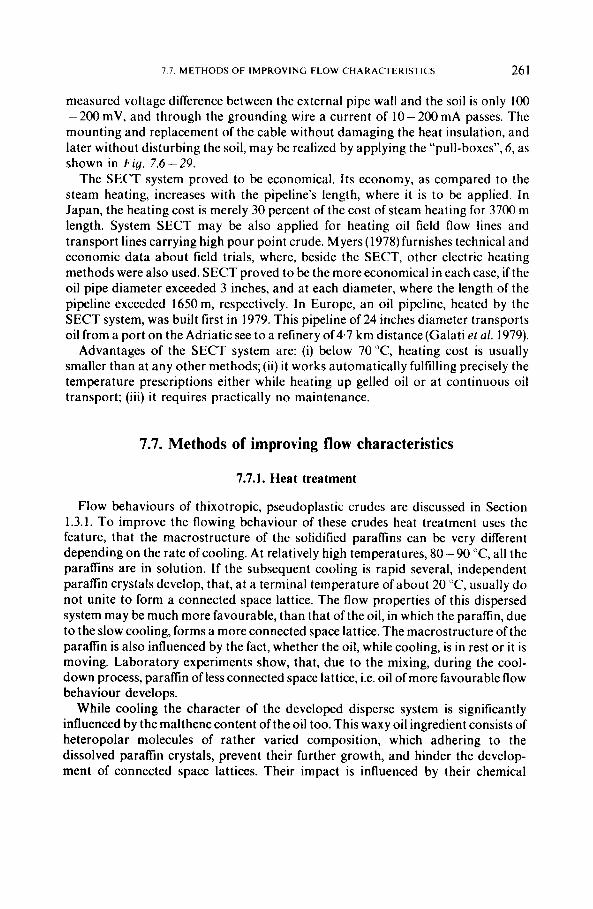
7.7. METHODS OF IMPROVING FLOW CHARACTERISTICS 26 1
measured voltage difference between the external pipe wall and the soil is only 100 -200 mV, and through the grounding wire a current of 10-200mA passes. The mounting and replacement of the cable without damaging the heat insulation, and later without disturbing the soil, may be realized by applying the "pull-boxes", 6, as shown in Fig. 7.6-29 .
The SECT system proved to be economical. Its economy, as compared to the steam heating, increases with the pipeline's length, where it is to be applied. In Japan, the heating cost is merely 30 percent of the cost of steam heating for 3700 m length. System SECT may be also applied for heating oil field flow lines and transport lines carrying high pour point crude. Myers (1978) furnishes technical and economic data about field trials, where, beside the SECT, other electric heating methods were also used. SECT proved to be the more economical in each case, if the oil pipe diameter exceeded 3 inches, and at each diameter, where the length of the pipeline exceeded 1650m, respectively. In Europe, an oil pipeline, heated by the SECT system, was built first in 1979. This pipeline of 24 inches diameter transports oil from a port on the Adriatic see to a refinery of4.7 km distance(Ga1ati et al. 1979).
Advantages of the SECT system are: (i) below 70°C, heating cost is usually smaller than at any other methods; (ii) it works automatically fulfilling precisely the temperature prescriptions either while heating up gelled oil or at continuous oil transport; (iii) it requires practically no maintenance.
7.7. Methods of improving flow characteristics
7.7.1. Heat treatment
Flow behaviours of thixotropic, pseudoplastic crudes are discussed in Section 1.3.1. To improve the flowing behaviour of these crudes heat treatment uses the feature, that the macrostructure of the solidified paraffins can be very different depending on the rate of cooling. At relatively high temperatures, 80- 90 "C, all the paraffins are in solution. If the subsequent cooling is rapid several, independent paraffin crystals develop, that, at a terminal temperature of about 20 "C, usually do not unite to form a connected space lattice. The flow properties of this dispersed system may be much more favourable, than that of the oil, in which the paraffin, due to the slow cooling, forms a more connected space lattice. The macrostructure of the paraffin is also influenced by the fact, whether the oil, while cooling, is in rest or i t is moving. Laboratory experiments show, that, due to the mixing, during the cool- down process, paraffin of less connected space lattice, i.e. oil of more favourable flow behaviour develops.
While cooling the character of the developed disperse system is significantly influenced by the malthene content of the oil too. This waxy oil ingredient consists of heteropolar molecules of rather varied composition, which adhering to the dissolved paraffin crystals, prevent their further growth, and hinder the develop- ment of connected space lattices. Their impact is influenced by their chemical
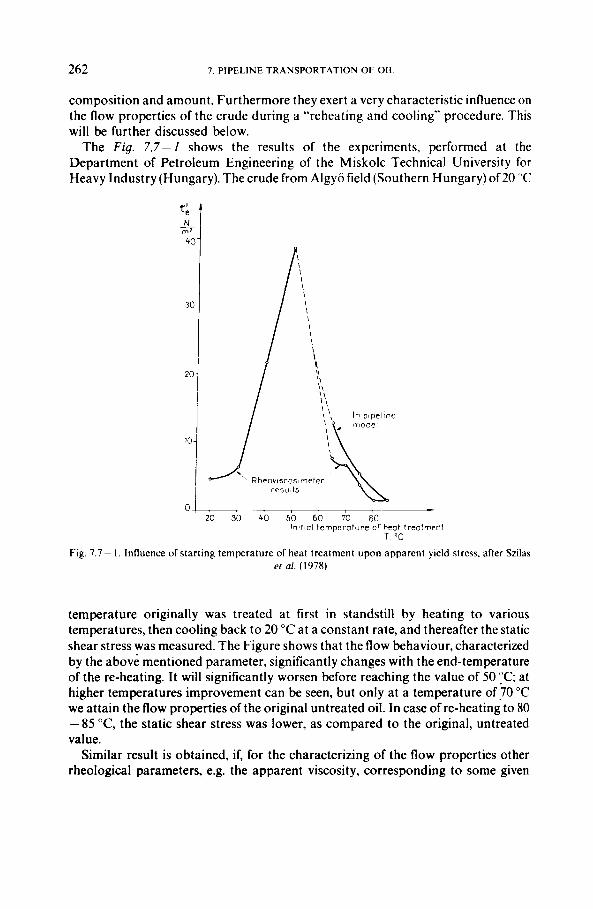
262 7. PIPELINE TRANSPORTATION OF OIL
7; N 77 40-
30
composition and amount. Furthermore they exert a very characteristic influence on the flow properties of the crude during a "reheating and cooling" procedure. This will be further discussed below.
The Fig. 7.7-1 shows the results of the experiments, performed at the Department of Petroleum Engineering of the Miskolc Technical University for Heavy Industry (Hungary). The crude from Algyo field (Southern Hungary) of 20 "C
'
PI I I I
20 30 40 50 60 70 80 Initial temperature o f heat treatrnenl
T "C
Fig. 7.7- 1. Influence of starting temperature of heat treatment upon apparent yield stress, after Szilas ef al. ( 1978)
temperature originally was treated at first in standstill by heating to various temperatures, then cooling back to 20 "C at a constant rate, and thereafter the static shear stress was measured. The Figure shows that the flow behaviour, characterized by the above mentioned parameter, significantly changes with the end-temperature of the re-heating. It will significantly worsen before reaching the value of 50 "c; at higher temperatures improvement can be seen, but only at a temperature of 70 "C we attain the flow properties of the original untreated oil. In case of re-heating to 80 - 8 5 "C, the static shear stress was lower, as compared to the original, untreated value.
Similar result is obtained, if, for the characterizing of the flow properties other rheological parameters, e.g. the apparent viscosity, corresponding to some given
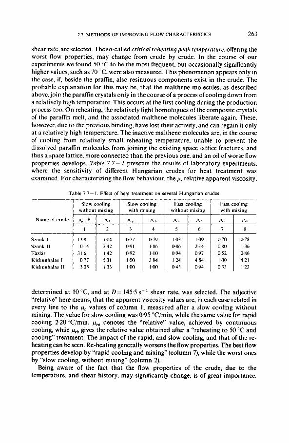
7.7. METHODS OF IMPROVING FLOW CHARACTERISTICS 263
Name of crude
Szank I Szank I I Tizlir Kiskunhalas I Kiskunhalas I I
shear rate, are selected. The so-called critical reheating peak temperature, offering the worst flow properties, may change from crude by crude. In the course of our experiments we found 50 “C to be the most frequent, but occasionally significantly higher values, such as 70 “C, were also measured. This phenomenon appears only in the case, if, beside the prafin, also resinuous components exist in the crude. The probable explanation for this may be, that the malthene molecules, as described above, join the paraffin crystals only in the course of a process of cooling down from a relatively high temperature. This occurs at the first cooling during the production process too. On reheating, the relatively light homologues of the composite crystals of the paraffin melt, and the associated malthene molecules liberate again. These, however, due to the previous binding, have lost their activity, and can regain it only at a relatively high temperature. The inactive malthene molecules are, in the course of cooling from relatively small reheating temperature, unable to prevent the dissolved paraffin molecules from joining the existing space lattice fractures, and thus a space lattice, more connected than the previous one, and an oil of worse flow properties develops. Table 7.7 - I presents the results of laboratory experiments, where the sensitivity of different Hungarian crudes for heat treatment was examined. For characterizing the flow behaviour, the p, relative apparent viscosity,
Slow cooling Slow cooling Fast cooling Fast cooling without mixing with mixing without mixing with mixing
p a , P p,h Pm P.h P.0 P r h P.“ P r b
1 2 3 4 5 6 7 8
13.8 1.04 0.77 0.79 1.03 1.09 0.70 0.78 0.14 242 0.91 1.86 0.86 2.14 0.80 1.36
31.6 1.42 092 1.10 0.94 0.97 0.52 0.86 0.77 5.31 1.00 3.84 1.24 4.84 1.00 4.21 3.05 1.33 1.00 1.00 0.43 0.94 0.33 1.22
Table 7.7- I . Effect of heat treatment on several Hungarian crudes
determined at 10 “C, and at D = 145.5 s - shear rate, was selected. The adjective “relative” here means, that the apparent viscosity values are, in each case related in every line to the pa values of column 1, measured after a slow cooling without mixing. The value for slow cooling was 095 “C/min, while the same value for rapid cooling 2.20 “C/min. pro denotes the “relative” value, achieved by continuous cooling, while prb gives the relative value obtained after a “reheating to 50 “C and cooling” treatment. The impact of the rapid, and slow cooling, and that of the re- heating can be seen. Re-heating generally worsens the flow properties. The best flow properties develop by “rapid cooling and mixing” (column 7), while the worst ones by “slow cooling, without mixing” (column 2).
Being aware of the fact that the flow properties of the crude, due to the temperature, and shear history, may significantly change, is of great importance.
264 7 PIPELINE TRANSPORTATION OF OIL
This knowledge may be directly used for industrial improvement of flow properties. Besides, it indicates, that also independently of our intentions, in the course of production, transport, and storage, the flow behaviour may change. Rheological measurements, the results of which may serve as a basis of the calculation of pressure loss, may be carried out only with representative samples, where the temperature and shear history is the same as that of the oil to be transported.
Both from the points of view of the laboratory-scale history simulation, and the heat treatment, performed in order to improve the flow properties, i t is important to determine the minimum and maximum efficient values for cooling speed. Maximum efficient cooling speed, expressed in "C/min units, is the limit value, above which the flow properties cannot be improved any more, while the minimum cooling speed is the value under which the flow properties already may not be worse. The above cooling speed values, occurring in practice range from 1 to 3"C/min. In the knowledge of these limits, on the onc hand, the time, required for the laboratory simulation of the flow history may be shortened, and, on the other hand, while designing the heat treatment process, the cooling speed, that enables us to achieve the most favourable flow properties by using the minimum cooling energy, may be determined.
By means of calculation it is generally impossible to determine the flow properties of a mixture of different thixotropic pseudoplastic crudes from the parameters of the basic oils. Beside the chemical composition of the components, the rate of their heat treatment. the temperatures of the components, and the difference in their temperatures before mixing play also an important role. The expectable flow properties may only be determined by measuring samples prepared by laboratory simulation of real shear and temperature history and mixing circumstances.
In certain cases simulation may be even more difficult, since the physico-chemical properties of the sample, during stopping or storage, may change. This phenomenon is called "aging", and is assumed to be related to changes in the chemical composition.
The first commercial application of heat treatment took place at Nahorkatiya and Moran, in India (Oil and Gas Journal 1963). Even today these are the largest heater-treater stations, described in literature, and they are modernized continuous- ly (Chandrasekharan and Sikdar 1970). The main parameters of the production and transport of the two oilfields, and the Nahorkatiya plant will be discussed as follows.
At Nahorkatiya, the crude whose pour point ranges from 29 to 34 "C and whose paraffin content is 15.4 percent, is transported through a 16" pipeline of 402 km length to a refinery where part of i t is refined; the rest is transported through a 1 4 ' line to another refinery at a distance of 765 km from the first one. The first line segment was designed for a yearly throughput of 2.75 Tg, the second for a throughput of 2.0 Tg year. The lowest soil temperature at pipe depth 1.2 - 1.8 m is 18 "C. Heat treatment is required between October and April. I t entails a significant improvement in flow behaviour. Typically, at 18 "C temperature and a shear rate of 13 s - I , the apparent viscosity is 0 6 Pas in untreated oil, and 0.1 Pas in treated oil.
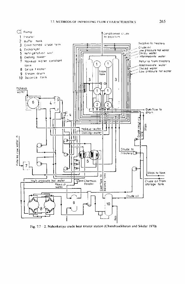
7.7. M E T H O D S OF I M P R O V I N G FLOW <'t1ARA('TI1RISTI~'S 265
2 3
Buffer tonh Condit ioned crude t o n k
4 Exchanger
5 Ref r i ge ra t i on un i t 6 cooling t ower
7 Makeup wa te r cons ton t
8 Selas h e a t e r
9 Steam d r u m 10 Balance rank
tCli7k
Mokeup m
Conditioned crude to boosters
7' I
r Suppltes to treaters
lntermediote woter
hot m t e r
Wokeup-water Cooling - water
. . , I - 1
3 1 - 1
Slops to tank
Crude oi l from storage tank
___e_
1 I Crude oil w
1"h Fig. 7.7- 2. Nahorkatiya crude heat treater station (Chandrasekharan and Sikdar 1970)
266 7. PIPELINE TRANSPORTATION OF 0 1 1
The Nahorkatiya crude heat treater plant is shown as Fig. 7.7-2 after Chandrasekharan and Sikdar (1970). The crude is heated in gas-fired heat- exchangers to between 90 and 95 “C. Subsequent cooling to 65 “C is effected in heat exchangers, using crude to be preheated as the coolant. In the next step, the static crude is chilled with water to 18 “C. Each of the 36 treater tanks is an upright cylindrical tank 6.1 m high, and of 9.2 m of diameter; each tank contains 127 one- inch chilling tubes. It is the cooling water that flows in the tubes, and the crude that occupies the space between them. Stationary cooling takes place in the following steps. The empty tank is filled with crude, which is chilled by the circulation of cold water at a rate ofO.6 “C/min. After cooling to 18 “C, the crude is pumped to a storage tank, and the tubes are used to circulate hot water, which again rises the tank temperature to 65 “C. This melts the deposited paraffin and prepares the tank for the reception of another batch of crude. These heating and cooling operations are performed by means of five water circiuts, each separate from the others. ( i ) High- pressure hot water heated with gas to 145 O C and held under sufficient pressure to keep it below its bubble point is used to heat low-pressure hot water and to regenerate the concentrated lithium bromide coolant of the absorption cooler. (ii) Low-pressure hot water is used to heat the treaters to 65 “C after the chilling period. (iii) “Intermediate” water is used to cool oil in the first phase ofcooling. I t is kept at a temperature of 30 “C by “cooling” water cooled in a cooling tower. (iv) Cold water is used to chill the crude to 18 “C in the treater tanks. This water is cooled to 14 “C in an absorption refrigerator. (v) Cooling water, circulated in an open circuit including a cooling tower, is used to cool the intermediate water. The 324 valves of the treating plant are controlled by an electric Flex-o-Timer. The water circuits are controlled by a programme controller which adjusts the required temperatures. The procedure, because of requiring a great investment, is rather expensive. That is why in India now a cheaper solution is being designed that provides continuous heat treatment during the flow (Mukhopadhyay 1979).
7.7.2. Solvent addition
The mixing together of two crudes, or products, comparatively low in malthenes, differring from each other in flow behaviour, will result in a mixture whose flow properties will usually fall between the properties of the two components. I t is possible to improve, by this means, the flow behaviour of high-paraffin, high viscosity gelling crudes, e.g. by the addition of lower viscosity crude, or a liquid product, such as gazoline, kerosene, or diesel fuel. Attempts have been made at predicting the behaviour of mixtures starting from those of the components. No laws of general scope have been derived as yet, but important research was carried out to determine empirical relationships (Aliev er al. 1969).
The effect of the solvent upon the continuous transport can be determined by measuring the flow curves of high viscosity crudes and those of the mixture at various temperatures, and from the results, in the way, described in Section 1.3.5, the change of the pressure gradient v. throughput at different temperatures is to be
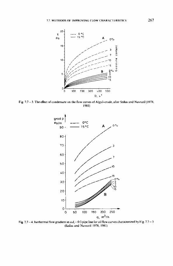
7.7. METHODS OF IMPROVING FLOW CHARACTERISTICS 267
0 100 Z M ) 300 400 500
D. s-’
Fig. 7.7- 3. The elTect of condensate on the flow curves of Algyo-crude, after Szilas and Navratil(1978, 1981)
grad P t
0 50 100 150 200 250
q , m 3 / h
Fig. 7.7-4. Isothermal flow gradient in a d i = 0.3 pipe line for oil flow curves characterized by Fig. 7.7 - 3 (Szilas and Navratil 1978, 1981)
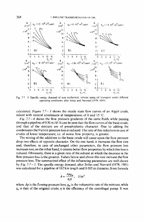
268 7. PIPELINE TRANSPORTATION OF OIL
A A A q, = I , O 1 0 ~ m ' / y e a r ,,m3 1 qa=1 .3 l o 6 m' lyear , / m 3 j q, = 1.5 l o 6 m ' i y e a r , / m 3 I
0 3 6 9 1 2 1 5 0 3 6 9 1 2 1 5 0 3 6 9 1 2 1 5 Tt 7 "C T t 1 'C Tt 3 'C
Fig. 7.7-5. Specific energy demand of non isothermal. solvent using oil transport under different operating conditions. after Szilas and Navratil (1978. 1981)
calculated. Figure 7.7-3 shows the steady state flow curves of an Algyo crude, mixed with natural condensate at temperatures of 0 and 15 "C.
Fig. 7.7-4 shows the flow pressure gradients of the same fluids while passing through a pipeline of0.30 m ID. I t can be seen that the flow curves of the basic crude, and that of the mixture are of pseudoplastic character. Due to adding the condensates the friction pressure loss is reduced. The rate of this reduction in case of crudes of lower temperature, i.e. of worse flow property, is greater.
The mixing of the additives to the basic crude will cause upon the flow pressure drop two effects of opposite character. On the one hand, it increases the flow rate and, therefore, in case of unchanged other parameters, the flow pressure loss increases too; on the other hand, it creates better flow properties by which this loss is reduced. Obviously, there is a given rate of the solvent at which the decrease in the flow pressure loss is the greatest. Values below and above this rate increase the flow pressure loss. The summarized effect of the influencing parameters are well shown by Fig. 7.7-5. The specific energy demand, after Szilas and Navratil (1978, 1981) was calculated for a pipeline of 162 km length and 0.305 m diameter, from formula
where A p is the flowing pressure loss; qm is the volumetric rate of the mixture, while qo is that of the original crude; is the efficiency of the centrifugal pump. It was
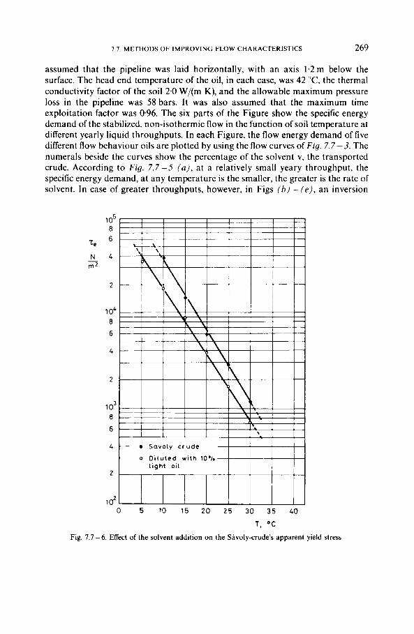
7.7. METHODS OF IMPROVING FLOW CHARACTERISTICS 269
assumed that the pipeline was laid horizontally, with an axis 1.2 m below the surface. The head end temperature of the oil, in each case, was 42 "C, the thermal conductivity factor of the soil 2.0 W/(m K), and the allowable maximum pressure loss in the pipeline was 58 bars. It was also assumed that the maximum time exploitation factor was 096. The six parts of the Figure show the specific energy demand of the stabilized, non-isothermic flow in the function of soil temperature at different yearly liquid throughputs. In each Figure, the flow energy demand of five different flow behaviour oils are plotted by using the flow curves of Fig. 7.7-3. The numerals beside the curves show the percentage of the solvent v, the transported crude. According to Fig. 7.7-5 ( a ) , at a relatively small yeary throughput, the specific energy demand, at any temperature is the smaller, the greater is the rate of solvent. In case of greater throughputs, however, in Figs ( h ) - ( e ) , an inversion
Sovo ly crude
0 5 10 15 20 25 30 35 40
1, o c
Fig. 7.7-6. Effect of the solvent addition on the Savoly-crude's apparent yield stress
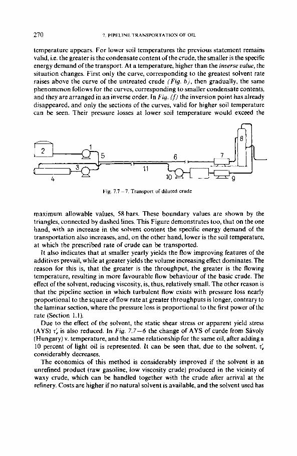
270 7. PIPELINE TRANSPORTATION OF OIL
temperature appears. For lower soil temperatures the previous statement remains valid, i.e. the greater is the condensate content of the crude, the smaller is the specific energy demand of the transport. At a temperature, higher than the inverse value, the situation changes. First only the curve, corresponding to the greatest solvent rate raises above the curve of the untreated crude ( F i g . b ) , then gradually, the same phenomenon follows for the curves, corresponding to smaller condensate contents, and they are arranged in an inverse order. In Fig. (f) the inversion point has already disappeared, and only the sections of the curves, valid for higher soil temperature can be seen. Their pressure losses at lower soil temperature would exceed the
Fig. 7.7 - 7. Transport of diluted crude
maximum allowable values, 58 bars. These boundary values are shown by the triangles, connected by dashed lines. This Figure demonstrates too, that on the one hand, with an increase in the solvent content the specific energy demand of the transportation also increases, and, on the other hand, lower is the soil temperature, at which the prescribed rate of crude can be transported.
I t also indicates that at smaller yearly yields the flow improving features of the additives prevail, while at greater yields the volume increasing effect dominates. The reason for this is, that the greater is the throughput, the greater is the flowing temperature, resulting in more favourable flow behaviour of the basic crude. The effect of the solvent, reducing viscosity, is, thus, relatively small. The other reason is that the pipeline section in which turbulent flow exists with pressure loss nearly proportional to the square of flow rate at greater throughputs is longer, contrary to the laminar section, where the pressure loss is proportional to the first power of the rate (Section 1.1).
Due to the effect of the solvent, the static shear stress or apparent yield stress (AYS) zi is also reduced. In Fig. 7.7-6 the change of AYS of curde from Savoly (Hungary) v. temperature, and the same relationship for the same oil, after adding a 10 percent of light oil is represented. It can be seen that, due to the solvent, rb considerably decreases.
The economics of this method is considerably improved if the solvent is an unrefined product (raw gasoline, low viscosity crude) produced in the vicinity of waxy crude, which can be handled together with the crude after arrival at the refinery. Costs are higher if no natural solvent is available, and the solvent used has
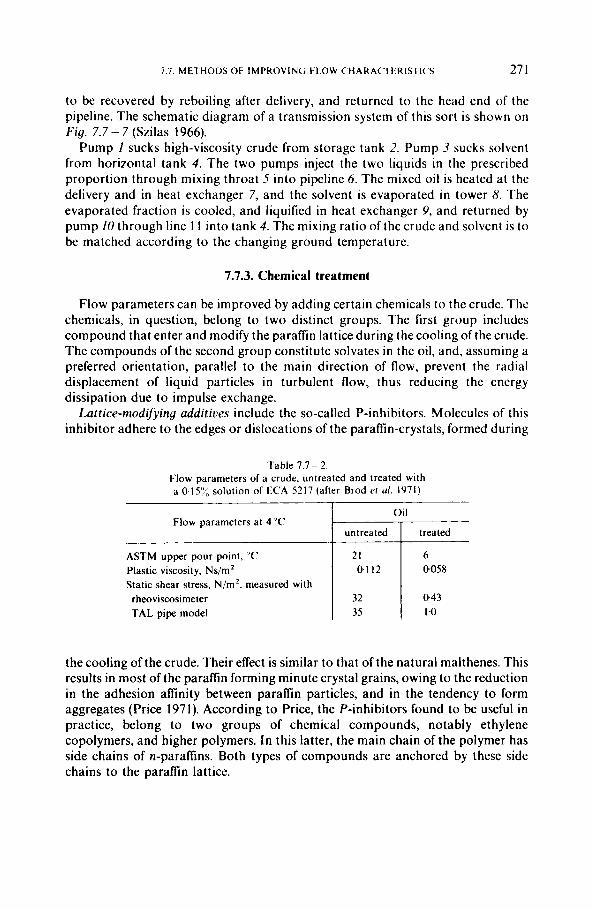
7.7. METHODS OF IMPROVING FLOW CHARACTERISTICS 27 1
Flow parameters at 4 “C
ASTM upper pour point, “C
Static shear stress, N/mZ, measured with Plastic viscosity, Ns/m2
rheoviscosimeter TAL pipe model
to be recovered by reboiling after delivery, and returned to the head end of the pipeline. The schematic diagram of a transmission system of this sort is shown on Fig. 7.7- 7 (Szilas 1966).
Pump I sucks high-viscosity crude from storage tank 2. Pump 3 sucks solvent from horizontal tank 4. The two pumps inject the two liquids in the prescribed proportion through mixing throat 5 into pipeline 6. The mixed oil is heated at the delivery and in heat exchanger 7, and the solvent is evaporated in tower 8. The evaporated fraction is cooled, and liquified in heat exchanger 9, and returned by pump 10 through line I 1 into tank 4. The mixing ratio of the crude and solvent is to be matched according to the changing ground temperature.
Oil
untreated treated
21 6 0.1 12 0.058
32 0.43 35 I .o
7.7.3. Chemical treatment
Flow parameters can be improved by adding certain chemicals to the crude. The chemicals, in question, belong to two distinct groups. The first group includes compound that enter and modify the paraffin lattice during the cooling of the crude. The compounds of the second group constitute solvates in the oil, and, assuming a preferred orientation, parallel to the main direction of flow, prevent the radial displacement of liquid particles in turbulent flow, thus reducing the energy dissipation due to impulse exchange.
Lattice-modijying additives include the so-called P-inhibitors. Molecules of this inhibitor adhere to the edges or dislocations of the paraffin-crystals, formed during
Table 7.7 - 2. Flow parameters of a crude, untreated and treated with a O.I5‘’< solution of ECA 5217 (after Brod el (I/. 1971)
the cooling of the crude. Their effect is similar to that of the natural malthenes. This results in most of the paraffin forming minute crystal grains, owing to the reduction in the adhesion affinity between paraffin particles, and in the tendency to form aggregates (Price 1971). According to Price, the P-inhibitors found to be useful in practice, belong to two groups of chemical compounds, notably ethylene copolymers, and higher polymers. In this latter, the main chain of the polymer has side chains of n-paraffins. Both types of compounds are anchored by these side chains to the paraffin lattice.
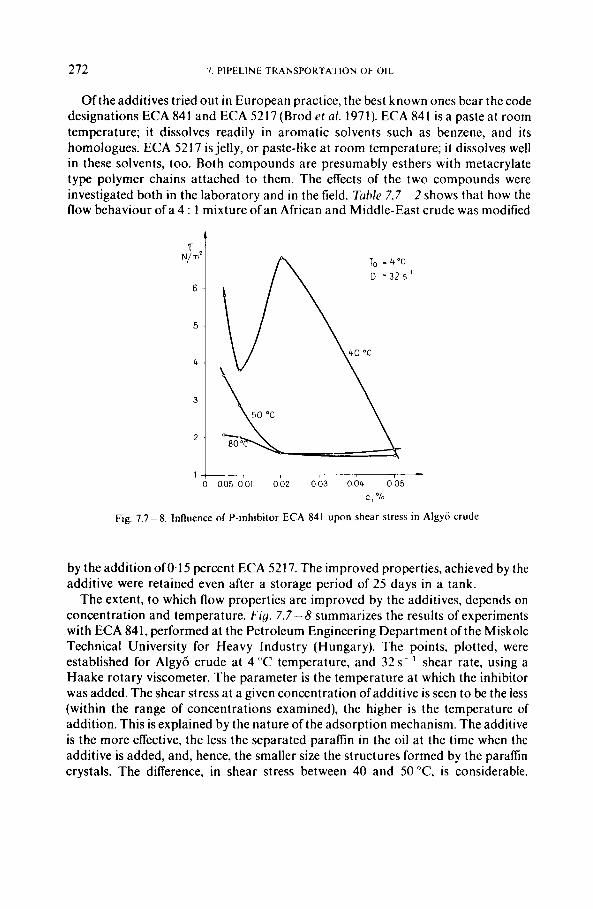
272 7. PIPELINE TRANSPORTATION OF 0 1 1 ,
'I N/m2
6 -
5 -
Ofthe additives tried out in European practice, the best known ones bear the code designations ECA 841 and ECA 5217 (Brod rt ul. 1971). ECA 841 is a paste at room temperature; it dissolves readily in aromatic solvents such as benzene, and its homologues. ECA 521 7 is jelly, or paste-like at room temperature; i t dissolves well in these solvents, too. Both compounds are presumably esthers with metacrylate type polymer chains attached to them. The effects of the two compounds were investigated both in the laboratory and in the field. Tuhle 7.7-2 shows that how the flow behaviour of a 4 : 1 mixture of an African and Middle-East crude was modified
4 -
3 -
2 -
-_T_) k 002 0 0 3 0 0 4 005 c , %
Fig. 7.7-8. Influence of P-Inhibitor ECA 841 upon shear stress in Algy6 crude
by the addition of0.15 percent ECA 5217. The improved properties, achieved by the additive were retained even after a storage period of 25 days in a tank.
The extent, to which flow properties are improved by the additives, depends on concentration and temperature. Fig. 7.7-8 summarizes the results of experiments with ECA 841, performed at the Petroleum Engineering Department of the Miskolc Technical University for Heavy Industry (Hungary). The points, plotted, were established for Algyo crude at 4 "C temperature, and 32 s - ' shear rate, using a Haake rotary viscometer. The parameter is the temperature at which the inhibitor was added. The shear stress at a given concentration of additive is seen to be the less (within the range of concentrations examined), the higher is the temperature of addition. This is explained by the nature of the adsorption mechanism. The additive is the more effective, the less the separated paraffin in the oil at the time when the additive is added, and, hence, the smaller size the structures formed by the paraffin crystals. The difference, in shear stress between 40 and 50"C, is considerable.
7 7 METHODS OF IMPROVING FLOW CHARACTERISTICS 273
Minimum shear stress was almost identical in the three cases. This value was ensured by adding just 0.02 weight percent ECA 841 at temperatures of 50 and 80 "C, whereas 0.05 percent was required to obtain the same effect at 40 C.
Laboratory tests are needed to decide which of the additives is efficient for a given crude, what is the optimum concentration and the optimum mixing temperature taking into account the economy too. Measuring the flow curves of the selected samples we can calculate the pressure gradient curves similar to those shown on Fig . 7 . 7 - 4 and so the friction pressure loss valid at given industrial transport parameters. It should be noted that the efficiency of the additives does not increase proportionally to the concentration. At several examined cases optimum efficiency could be achieved at relatively small, 0.025 -0.05 percent of concentration.
In the oil production and transport practice several methods are known by which the adhesion of the paraffin on the inner wall of the pipe, dissolved from the crude, may be partially, or fully prevented. A group of these methods, in order to achieve the prescribed aim, uses chemicals. Fulford ( 1975) describes investigations, where the efficiency of this type of chemicals was determined by laboratory-scale flow experiments. He found that the optimum values were achieved with five ethylene co- polymers of different composition. We may assume that these chemicals may modify the space lattice, and thus, their mechanism of operation is very similar to that of the P-inhibitors.
It was in 1954 that drag reduction in both Newtonian and non-Newtonian fluids under the influence ofcertain additives was first observed. Experience has shown the most effective drag reducers to be long straight-chained lyophilic polymers. In polar liquids, e.g. water, the most effective molecules are those which include polar groups such as the carboxy group. One such compound is CMC (carboxy-methyl- cellulose). These macromolecules form solvates in the fluid to which they are added (Elperin et al. 1966). In the oil industry, drag-reducing additives are added mainly to the water-based injection fluids of hydraulic formation fracturing. Lescarboura et al. (1970) describe that both laboratory and field experiments were carried out in Oklahoma in order to determine, that, for decreasing the frictional pressure loss in the light oil, and Diesel oil, respectively, what additive, and to what a proportion, may be efficient. The additives tested included the high-molecular-weight hydrocarbon polymer of code designation CDR, and several variants of a polysobuthylene, called Vistanex. At a given concentration, these additives were found to be the more effective, the more readily they solvate in the fluid to be treated. The presence of polymers may reduce the drag in turbulent flow in two ways. In the flowing liquid, the elastic macromolecules arranged parallel to the flow direction hinder the radial movement of the flowing liquid's particles, and adsorb and temporarily store the energy that would otherwise get dissipated by impulse exchange (Pruitt et al. 1965). The other effect, involved, is that some.of the macromolecules will adhere to the pipe wall, and reduce its relative roughness (White 1964). The presence of the polymers augments the apparent viscosity of the transported liquid, and imparts non-Newtonian properties even to Newtonian
I8
274 7. PIPELINE TRANSPORTATION OF. OIL
fluids. A very comprehensive survey of the different ideas concerning the effect of the different additives is given by Hoyt (1972).
The pressure drop to be expected in a pipeline cannot be predicted on the basis of flow curves determined by means of rotary viscometer. That is due to two factors. One, the rotation viscometer will not evaluate the influence of pipe roughness. Two, according to certain hypotheses(E1perin et al. 1966) flow in the pipe may arrange the polymer molecules so. that their concentration will differ from the axis to the pipe wall. Wang (1972) carried out flow experiments in laboratory size pipelines. He wanted to find, that how the two types of friction reducing additives would change the friction factor, valid for the clean basic oil. The equation, derived on the basis of his experiments, is practically a generalized version of the Prandtl-Kirmin equation, 1. I - 6
7.7- I
where B is the factor of the friction loss reducing additive, that can be obtained from the formula:
8=0’288 B,,, Ig (7’4T,,,/TWc). 7.7-2
B,,, is the maximum value of B factor, realizable by the given additives, that can be determined by laboratory-scale pipeline experiments, in the function of the factor (p, -pb) /pm that includes the dynamic viscosities of the basic oil, and the mixture. The viscosity of the mixture, p,,, is always higher than that of the basic oil, p,, , and its magnitude is proportional to the concentration. Its value may be measured by extrusion viscometer. 5, is the shear stress, prevailing at the pipe wall, and T,, is the shear stress prevailing at the pipe wall, that develops if factor B is just the half of the value of B,,, . The application of the above relation requires laboratory experiments, that are not available for every designers. The knowledge of an equation, from which the expected effect of the additive may be approximately calculated, may be, thus, important too. Such relation is described by Lescarboura et al. ( 1 970).
Strictly, this procedure holds only for the fluids and additives tested, but it will give a rough idea of what to expect with other fluids and additives, and permits to estimate the extent of drag reduction. Laboratory experiments were performed in one-in. pipe of 3.7 m length, in a flow velocity range from 0.6 -4.9 m/s. These were succeeded by field experiments in 45 km of 8” and 51.5 km of 12” line respectively. I t was found that the drag reduction Apdr/Ap, due to a given additive in a given fluid depends on the additive concentration cdr , flow velocity u, and pipe diameter di . The drag reduction due to the additive, termed CDR, in the 8” and 12” pipes tested (and, in a fair approximation, all over the pipe size range from 4 - 16”) is
1 ~ = 2 Ig N , , $-0.8+ B , 45
‘Pdr - 2.19 V - 1
A P O CdrV
- lo00 ’ +
032cdr - 309 76.6 + 0 . 0 9 8 ~ ~ ~
where Cdr is the additive concentration in parts per million ( m3/m3),
7.7 - 3
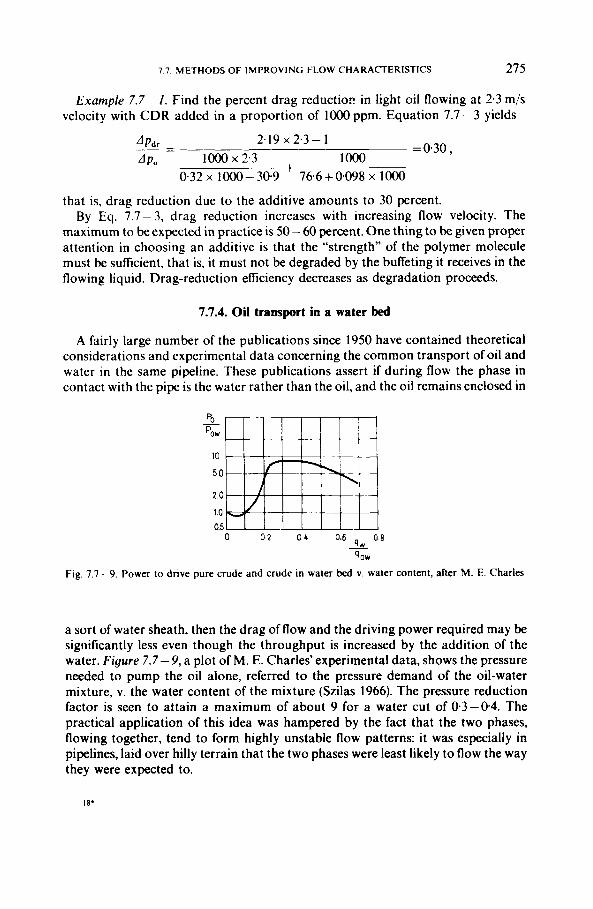
7.7. METHODS OF IMPROVING FLOW CHARACTERISTICS 275
Example 7.7- 1. Find the percent drag reductior! in light oil flowing at 2.3 m/s velocity with CDR added in a proportion of lo00 ppm. Equation 7.7 - 3 yields
2.19 x 2.3- 1 = 0.30 , APdr - --
AD, lo00 x 2.3 lo00 + . ” 0.32 x 1 OOO - 30.9 76.6 + 0.098 x 1 o00
that is, drag reduction due to the additive amounts to 30 percent. By Eq. 7.7-3, drag reduction increases with increasing flow velocity. The
maximum to be expected in practice is 50 - 60 percent. One thing to be given proper attention in choosing an additive is that the “strength of the polymer molecule must be sufficient, that is, i t must not be degraded by the buffeting it receives in the flowing liquid. Drag-reduction efficiency decreases as degradation proceeds.
7.7.4. Oil transport in a water bed
A fairly large number of the publications since 1950 have contained theoretical considerations and experimental data concerning the common transport of oil and water in the same pipeline. These publications assert if during flow the phase in contact with the pipe is the water rather than the oil, and the oil remains enclosed in
0 0 2 04 0.6 08 - qw
qow
Fig. 7.7 -9. Power to dnve pure crude and crude in water bed v. water content, after M. E. Charles
a sort of water sheath, then the drag of flow and the driving power required may be significantly less even though the throughput is increased by the addition of the water. Figure 7.7-9, a plot of M. E. Charles’experimental data, shows the pressure needed to pump the oil alone, referred to the pressure demand of the oil-water mixture, v. the water content of the mixture (Szilas 1966). The pressure reduction factor is seen to attain a maximum of about 9 for a water cut of 0.3-04. The practical application of this idea was hampered by the fact that the two phases, flowing together, tend to form highly unstable flow patterns: it was especially in pipelines, laid over hilly terrain that the two phases were least likely to flow the way they were expected to.
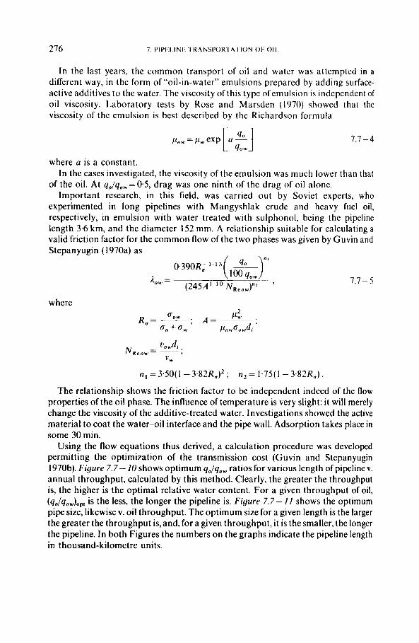
276 7. P I P E L I N E TRANSPORTATION or.. 011
In the last years, the common transport of oil and water was attempted in a different way, in the form of "oil-in-water" emulsions prepared by adding surface- active additives to the water. The viscosity of this type of emulsion is independent of oil viscosity. Laboratory tests by Rose and Marsden (1970) showed that the viscosity of the emulsion is best described by the Richardson formula
7.7 -4
where a is a constant. In the cases investigated, the viscosity of the emulsion was much lower than that
of the oil. At qo/qow=0.5, drag was one ninth of the drag of oil alone. Important research, in this field, was carried out by Soviet experts, who
experimented in long pipelines with Mangyshlak crude and heavy fuel oil, respectively, in emulsion with water treated with sulphonol, being the pipeline length 3 6 km, and the diameter 152 mm. A relationship suitable for calculating a valid friction factor for the common flow of the two phases was given by Guvin and Stepanyugin (l970a) as
7.1 - 5
where
The relationship shows the friction factor to be independent indeed of the flow properties of the oil phase. The influence of temperature is very slight: i t will merely change the viscosity of the additive-treated water. Investigations showed the active material to coat the water-oil interface and the pipe wall. Adsorption takes place in some 30 min.
Using the flow equations thus derived, a calculation procedure was developed permitting the optimization of the transmission cost (Guvin and Stepanyugin 1970b). Figure 7.7- I0 shows optimum qo/qow ratios for various length of pipeline v. annual throughput, calculated by this method. Clearly, the greater the throughput is, the higher is the optimal relative water content. For a given throughput of oil, (qo/qow)op, is the less, the longer the pipeline is. Figure 7 . 7 - / I shows the optimum pipe size, likewise v. oil throughput. The optimum size for a given length is the larger the greater the throughput is, and, for a given throughput, it is the smaller, the longer the pipeline. In both Figures the numbers on the graphs indicate the pipeline length in thousand-kilometre units.
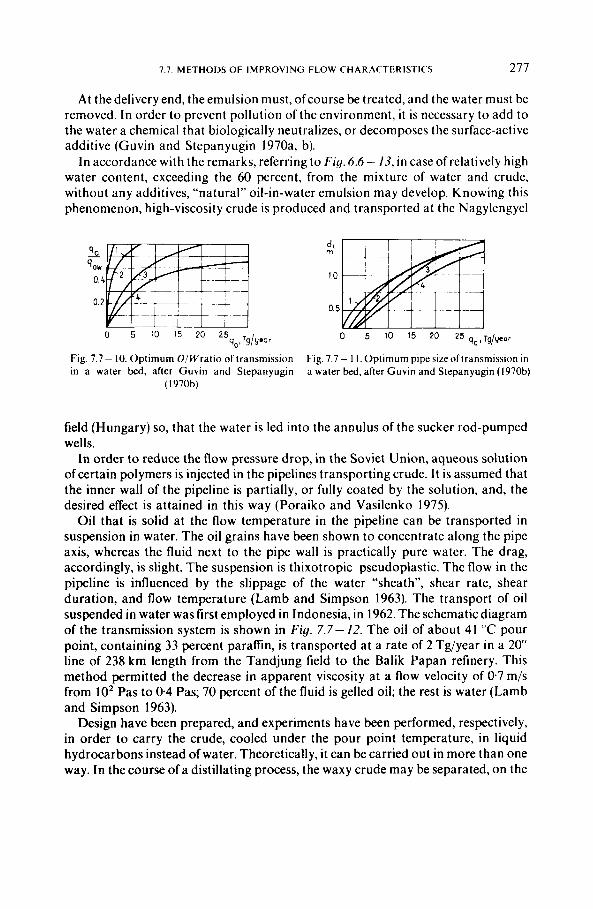
7.7. METHODS OF IMPROVING FLOW CHARACTERISTICS 277
At the delivery end, the emulsion must, ofcourse be treated, and the water must be removed. In order to prevent pollution of the environment, i t is necessary to add to the water a chemical that biologically neutralizes, or decomposes the surface-active additive (Guvin and Stepanyugin 1970a, b).
In accordance with the remarks, referring to Fig. 6.6 - 13, in case of relatively high water content, exceeding the 60 percent, from the mixture of water and crude, without any additives, “natural” oil-in-water emulsion may develop. Knowing this phenomenon, high-viscosity crude is produced and transported at the Nagylcngyel
- 90
q o w 0 4
0 2
0 5 lo l5 *O 25 q,,,Tg/yeor
Fig. 7.7- 10. Optimum OIWratio of transmission in a water bed, after Guvin and Stepanyugin
( I 970b)
Fig. 7.7- 1 I . Optimum pipe sizeoftransmission in a water bed, after Guvin and Stepanyugin (1970b)
field (Hungary) so, that the water is led into the annulus of the sucker rod-pumped wells.
In order to reduce the flow pressure drop, in the Soviet Union, aqueous solution of certain polymers is injected in the pipelines transporting crude. I t is assumed that the inner wall of the pipeline is partially, or fully coated by the solution, and, the desired effect is attained in this way (Poraiko and Vasilenko 1975).
Oil that is solid at the flow temperature in the pipeline can be transported in suspension in water. The oil grains have been shown to concentrate along the pipe axis, whereas the fluid next to the pipe wall is practically pure water. The drag, accordingly, is slight. The suspension is thixotropic-pseudoplastic. The flow in the pipeline is influenced by the slippage of the water “sheath”, shear rate, shear duration, and flow temperature (Lamb and Simpson 1963). The transport of oil suspended in water was first employed in Indonesia, in 1962. The schematic diagram of the transmission system is shown in Fig. 7.7- f2. The oil of about 41 “C pour point, containing 33 percent paraflin, is transported at a rate of 2 Tg/year in a 20’ line of 238 km length from the Tandjung field to the Balik Papan refinery. This method permitted the decrease in apparent viscosity at a flow velocity of 0 7 m/s from 10’ Pas to 0.4 Pas; 70 percent of the fluid is gelled oil; the rest is water (Lamb and Simpson 1963).
Design have been prepared, and experiments have been performed, respectively, in order to carry the crude, cooled under the pour point temperature, in liquid hydrocarbons instead of water. Theoretically, it can be carried out in more than one way. In the course of a distillating process, the waxy crude may be separated, on the
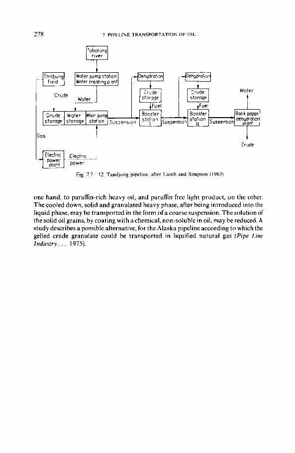
278
Booster Booster Bolik papan
7. PIPELINE TRANSPORTATION OF OIL
p g ""."","'""""I Water treating plant
Crude Water
I I
Dehydrotio
Crude Crude Water
storage f
i Crude
Fig. 7 . 7 - 12. Tandjung pipeline. after Lamb and Sirnpson (1963)
one hand, to parafin-rich heavy oil, and parafin free light product, on the other. The cooled down, solid and granulated heavy phase, after being introduced into the liquid phase, may be transported in the form of a coarse suspension. The solution of the solid oil grains, by coating with a chemical, non-soluble in oil, may be reduced. A study describes a possible alternative, for the Alaska pipeline according to which the gelled crude granulate could be transported in liquified natural gas (Pipe Line Industry. . . 1975).


![Cost of pipeline transportation [autosaved]](https://img.pdfslide.tips/doc/110x75/54677733af79599b108b551f/cost-of-pipeline-transportation-autosaved.jpg)