Embed Size (px)
Citation preview
Point-Based Computer Graphics
Eurographics 2003 Tutorial T1
Organizers
Markus Gross ETH Zürich
Hanspeter Pfister
MERL, Cambridge
Presenters
Marc Alexa TU Darmstadt
Carsten Dachsbacher
Universität Erlangen-Nürnberg
Markus Gross ETH Zürich
Mark Pauly ETH Zürich
Jeroen van Baar
MERL, Cambridge
Matthias Zwicker ETH Zürich

2
Contents
Tutorial Schedule ................................................................................................2 Presenters and Organizers Contact Information .................................................3 References ...........................................................................................................4 Project Pages .......................................................................................................5
Tutorial Schedule
Introduction (Markus Gross) Acquisition of Point-Sampled Geometry and Appearance (Jeroen van Baar) Point-Based Surface Representations (Marc Alexa) Point-Based Rendering (Matthias Zwicker) Lunch Sequential Point Trees (Carsten Dachsbacher) Efficient Simplification of Point-Sampled Geometry (Mark Pauly) Spectral Processing of Point-Sampled Geometry (Markus Gross) Pointshop3D: A Framework for Interactive Editing of Point-Sampled Surfaces (Markus Gross) Shape Modeling (Mark Pauly) Pointshop3D Demo (Mark Pauly) Discussion (all)

3
Presenters and Organizers Contact Information
Dr. Markus Gross Professor Department of Computer Science Swiss Federal Institute of Technology (ETH) CH 8092 Zürich Switzerland Phone: +41 1 632 7114 FAX: +41 1 632 1596 [email protected] http://graphics.ethz.ch
Dr. Hanspeter Pfister Associate Director MERL - A Mitsubishi Electric Research Lab 201 Broadway Cambridge, MA 02139 USA Phone: (617) 621-7566 Fax: (617) 621-7550 [email protected] http://www.merl.com/people/pfister/ Jeroen van Baar MERL - A Mitsubishi Electric Research Lab 201 Broadway Cambridge, MA 02139 USA Phone: (617) 621-7577 Fax: (617) 621-7550 [email protected] http://www.merl.com/people/jeroen/ Matthias Zwicker Department of Computer Science Swiss Federal Institute of Technology (ETH) CH 8092 Zürich Switzerland Phone: +41 1 632 7437 FAX: +41 1 632 1596 [email protected] http://graphics.ethz.ch
Mark Pauly Department of Computer Science Swiss Federal Institute of Technology (ETH) CH 8092 Zürich

4
Switzerland Phone: +41 1 632 0906 FAX: +41 1 632 1596 [email protected] http://graphics.ethz.ch
Dr. Marc Stamminger Universität Erlangen-Nürnberg Am Weichselgarten 9 91058 Erlangen Germany Phone: +49 9131 852 9919 FAX: +49 9131 852 9931 [email protected]
Carsten Dachsbacher Universität Erlangen-Nürnberg Am Weichselgarten 9 91058 Erlangen Germany Phone: +49 9131 852 9925 FAX: +49 9131 852 9931 [email protected]
Dr. Marc Alexa Interactive Graphics Systems Group Technische Universität Darmstadt Fraunhoferstr. 5 64283 Darmstadt Germany Phone: +49 6151 155 674 FAX: +49 6151 155 669 [email protected] http://www.dgm.informatik.tu-darmstadt.de/staff/alexa/
References
M. Alexa, J. Behr, D. Cohen-Or, S. Fleishman, D. Levin, C. Silva. Point set surfaces. Proceedings of IEEE Visualization 2001, p. 21-28, San Diego, CA, October 2001. C. Dachsbacher, C. Vogelsang, M. Stamminger, Sequential point trees. Proceedings of SIGGRAPH 2003, to appear, San Diego, CA, July 2003. O. Deussen, C. Colditz, M. Stamminger, G. Drettakis, Interactive visualization of complex plant ecosystems. Proceedings of IEEE Visualization 2002, Boston, MA, October 2002.
5
W. Matusik, H. Pfister, P. Beardsley, A. Ngan, R. Ziegler, L. McMillan, Image-based 3D photography using opacity hulls. Proceedings of SIGGRAPH 2002, San Antonio, TX, July 2002. W. Matusik, H. Pfister, A. Ngan, R. Ziegler, L. McMillan, Acquisition and rendering of transparent and refractive objects. Thirteenth Eurographics Workshop on Rendering, Pisa, Italy, June 2002. M. Pauly, R. Keiser, L. Kobbelt, M. Gross, Shape modelling with point-sampled geometry, to appear, Proceedings of SIGGRAPH 2003, San Diego, CA, July 2003.
M. Pauly, M. Gross, Spectral processing of point-sampled geometry. Proceedings of SIGGRAPH 2001, p. 379-386, Los Angeles, CA, August 2001. M. Pauly, M. Gross, Efficient Simplification of Point-Sampled Surfaces. IEEE Proceedings of Visualization 2002, Boston, MA, October 2002. H. Pfister, M. Zwicker, J. van Baar, M. Gross, Surfels - surface elements as rendering primitives. Proceedings of SIGGRAPH 2000, p. 335-342, New Orleans, LS, July 2000. M. Stamminger, G. Drettakis, Interactive sampling and rendering for complex and procedural geometry, Rendering Techniques 2001, Proceedings of the Eurographics Workshop on Rendering 2001, June 2001. L. Ren, H. Pfister, M. Zwicker, Object space EWA splatting: a hardware accelerated approach to high quality point rendering. Proceedings of the Eurographics 2002, to appear, Saarbrücken, Germany, September 2002. M. Zwicker, H. Pfister, J. van Baar, M. Gross, EWA volume splatting. Proceedings of IEEE Visualization 2001, p. 29-36, San Diego, CA, October 2001. M. Zwicker, H. Pfister, J. van Baar, M. Gross, Surface splatting. Proceedings of SIGGRAPH 2001, p. 371-378, Los Angeles, CA, August 2001. M. Zwicker, H. Pfister, J. van Baar, M. Gross, EWA splatting. IEEE Transactions on Visualization and Computer Graphics. M. Zwicker, M. Pauly, O. Knoll, M. Gross, Pointshop 3D: an interactive system for point-based surface editing. Proceedings of SIGGRAPH 2002, San Antonio, TX, July 2002
Project Pages
• Rendering http://graphics.ethz.ch/surfels
• Acquisition http://www.merl.com/projects/3Dimages/

6
• Sequential point trees http://www9.informatik.uni-erlangen.de/Persons/Stamminger/Research
• Modeling, processing, sampling and filtering http://graphics.ethz.ch/points
• Pointshop3D http://www.pointshop3d.com
1
Point-Based Computer GraphicsTutorial T1
Marc Alexa, Carsten Dachsbacher, Markus Gross, Mark Pauly,
Hanspeter Pfister, Marc Stamminger, Jeroen Van Baar, Matthias Zwicker
2Point-Based Computer Graphics Markus Gross
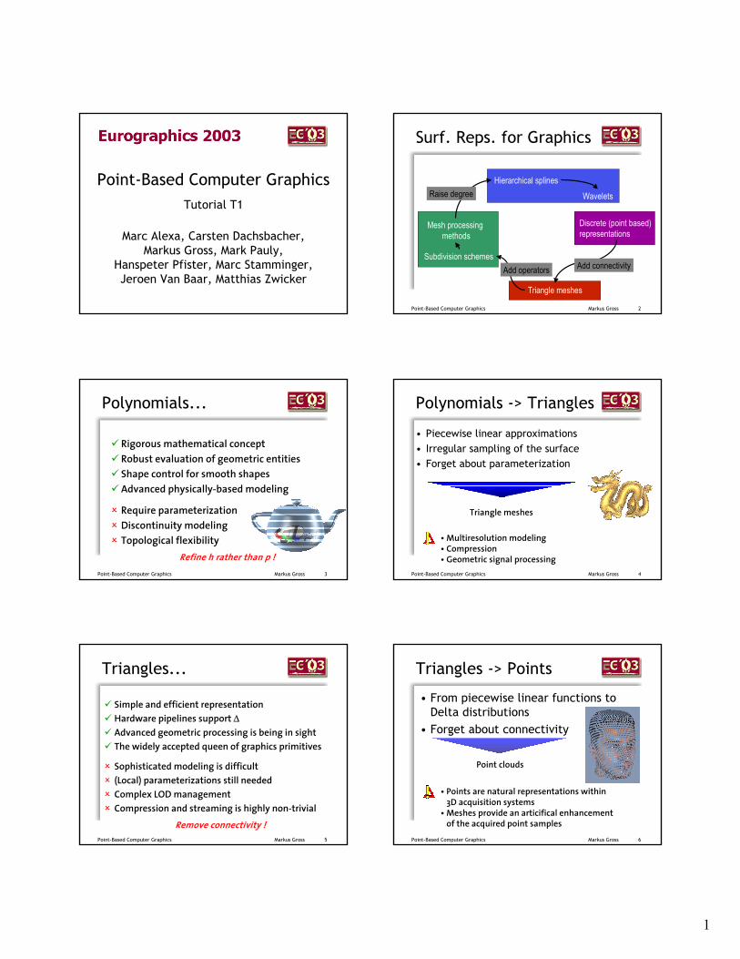
Surf. Reps. for Graphics
Hierarchical splines
Wavelets
Subdivision schemes
Triangle meshes
Mesh processingmethods
Discrete (point based) representations
Add connectivityAdd operators
Raise degree
3Point-Based Computer Graphics Markus Gross
Polynomials...
Rigorous mathematical conceptRobust evaluation of geometric entitiesShape control for smooth shapesAdvanced physically-based modeling
Require parameterizationDiscontinuity modelingTopological flexibility
Refine h rather than p !4Point-Based Computer Graphics Markus Gross
Polynomials -> Triangles
• Piecewise linear approximations• Irregular sampling of the surface• Forget about parameterization
Triangle meshes
• Multiresolution modeling• Compression• Geometric signal processing
5Point-Based Computer Graphics Markus Gross
Triangles...
Simple and efficient representation Hardware pipelines support ∆Advanced geometric processing is being in sightThe widely accepted queen of graphics primitives
Sophisticated modeling is difficult(Local) parameterizations still neededComplex LOD managementCompression and streaming is highly non-trivial
Remove connectivity !6Point-Based Computer Graphics Markus Gross
Triangles -> Points
• From piecewise linear functions to Delta distributions
• Forget about connectivity
Point clouds
• Points are natural representations within 3D acquisition systems
• Meshes provide an articifical enhancement of the acquired point samples

2
7Point-Based Computer Graphics Markus Gross
History of Points in Graphics• Particle systems [Reeves 1983]• Points as a display primitive [Whitted, Levoy 1985]• Oriented particles [Szeliski, Tonnesen 1992]• Particles and implicit surfaces [Witkin, Heckbert 1994]• Digital Michelangelo [Levoy et al. 2000]• Image based visual hulls [Matusik 2000]• Surfels [Pfister et al. 2000]• QSplat [Rusinkiewicz, Levoy 2000]• Point set surfaces [Alexa et al. 2001]• Radial basis functions [Carr et al. 2001]• Surface splatting [Zwicker et al. 2001]• Randomized z-buffer [Wand et al. 2001]• Sampling [Stamminger, Drettakis 2001]• Opacity hulls [Matusik et al. 2002]• Pointshop3D [Zwicker, Pauly, Knoll, Gross 2002]...?
8Point-Based Computer Graphics Markus Gross
The Purpose of our Course is …
I) …to introduce points as a versatile and powerful graphics primitive
II) …to present state of the art concepts for acquisition, representation, processing and rendering of point sampled geometry
III) …to stimulate YOU to help us to further develop Point Based Graphics
9Point-Based Computer Graphics Markus Gross
Taxonomy
Point-Based Graphics
Rendering(Zwicker)
Acquisition(Pfister, Stamminger)
Processing &Editing
(Gross, Pauly)Representation
(Alexa)
10Point-Based Computer Graphics Markus Gross
Morning Schedule
• Introduction (Markus Gross)• Acquisition of Point-Sampled Geometry and
Apprearance (Jeroen van Baar)• Point-Based Surface Representations (Marc
Alexa)• Point-Based Rendering (Matthias Zwicker)
11Point-Based Computer Graphics Markus Gross
Afternoon Schedule
• Sequential point trees (Carsten Dachsbacher)• Efficient simplification of point-sampled geometry
(Mark Pauly)• Spectral processing of point-sampled geometry
(Markus Gross)• Pointshop3D: A framework for interactive editing
of point-sampled surfaces (Markus Gross)• Shape modeling (Mark Pauly)• Pointshop3D demo (Mark Pauly)• Discussion (all)

Point-Based Computer Graphics Hanspeter Pfister, MERL 1
Acquisition of Point-Sampled Geometry and Appearance
Jeroen van Baar and Hanspeter Pfister, MERL[jeroen,pfister]@merl.com
Wojciech Matusik, MITAddy Ngan, MIT
Paul Beardsley, MERLRemo Ziegler, MERL
Leonard McMillan, MIT
Point-Based Computer Graphics Hanspeter Pfister, MERL 2
The Goal: To Capture Reality
• Fully-automated 3D model creation of real objects.
• Faithful representation of appearance for these objects.
Point-Based Computer Graphics Hanspeter Pfister, MERL 3
Image-Based 3D Photography
• An image-based 3D scanning system.• Handles fuzzy, refractive, transparent objects.• Robust, automatic• Point-sampled geometry based on the visual hull.• Objects can be rendered in novel environments.
Point-Based Computer Graphics Hanspeter Pfister, MERL 4
Previous Work
• Active and passive 3D scanners• Work best for diffuse materials.• Fuzzy, transparent, and refractive objects are difficult.
• BRDF estimation, inverse rendering• Image based modeling and rendering
• Reflectance fields [Debevec et al. 00]
• Light Stage system to capture reflectance fields• Fixed viewpoint, no geometry
• Environment matting [Zongker et al. 99, Chuang et al. 00]
• Capture reflections and refractions• Fixed viewpoint, no geometry
Point-Based Computer Graphics Hanspeter Pfister, MERL 5
Outline
• OverviewSystem
• Geometry• Reflectance• Refraction & Transparency
Point-Based Computer Graphics Hanspeter Pfister, MERL 6
Acquisition System
Mul
ti-C
olor
Mon
itor
Light Array
Cameras
Rotating Platform
Point-Based Computer Graphics Hanspeter Pfister, MERL 7
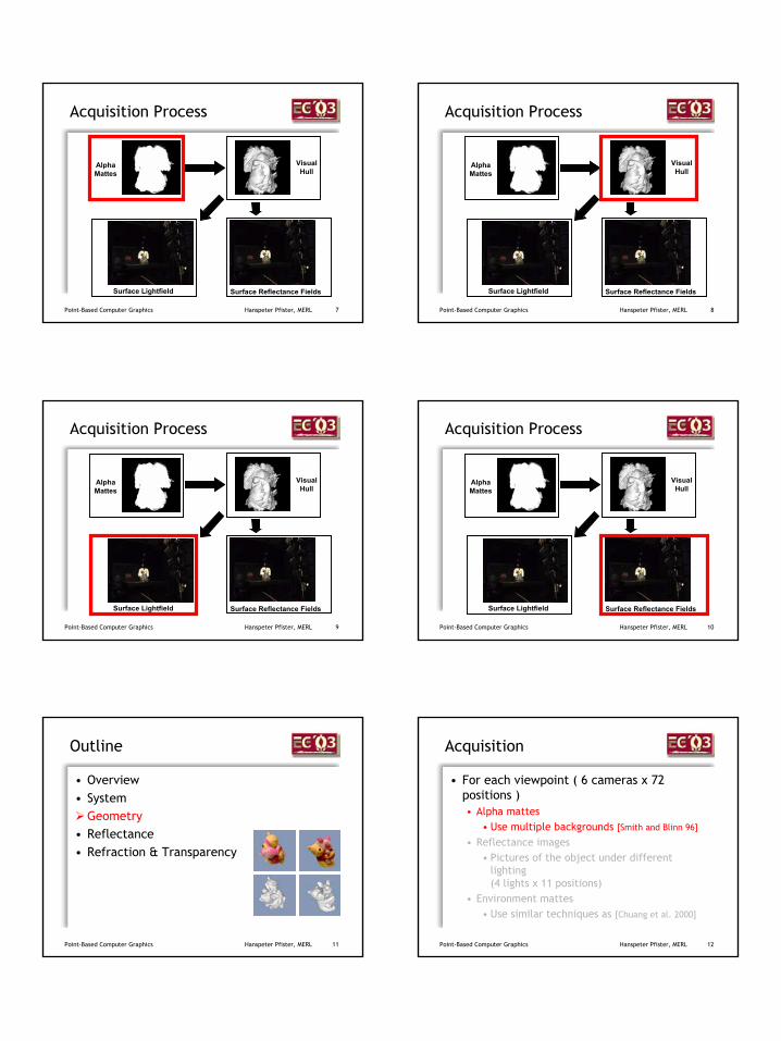
Acquisition Process
Alpha Mattes
VisualHull
Surface Lightfield Surface Reflectance Fields
Point-Based Computer Graphics Hanspeter Pfister, MERL 8
Acquisition Process
Alpha Mattes
VisualHull
Surface Lightfield Surface Reflectance Fields
Point-Based Computer Graphics Hanspeter Pfister, MERL 9
Acquisition Process
Alpha Mattes
VisualHull
Surface Lightfield Surface Reflectance Fields
Point-Based Computer Graphics Hanspeter Pfister, MERL 10
Acquisition Process
Alpha Mattes
VisualHull
Surface Lightfield Surface Reflectance Fields
Point-Based Computer Graphics Hanspeter Pfister, MERL 11
Outline
• Overview• System
Geometry• Reflectance• Refraction & Transparency
Point-Based Computer Graphics Hanspeter Pfister, MERL 12
Acquisition
• For each viewpoint ( 6 cameras x 72 positions )• Alpha mattes
• Use multiple backgrounds [Smith and Blinn 96]
• Reflectance images• Pictures of the object under different
lighting (4 lights x 11 positions)
• Environment mattes• Use similar techniques as [Chuang et al. 2000]
Point-Based Computer Graphics Hanspeter Pfister, MERL 13
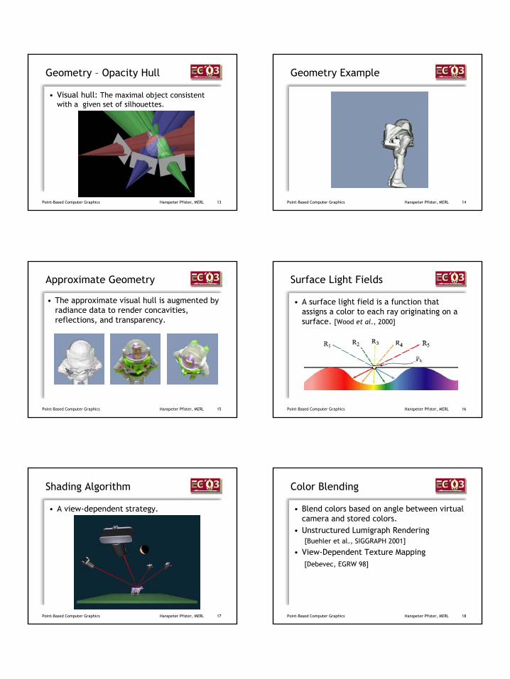
Geometry – Opacity Hull
• Visual hull: The maximal object consistent with a given set of silhouettes.
Point-Based Computer Graphics Hanspeter Pfister, MERL 14
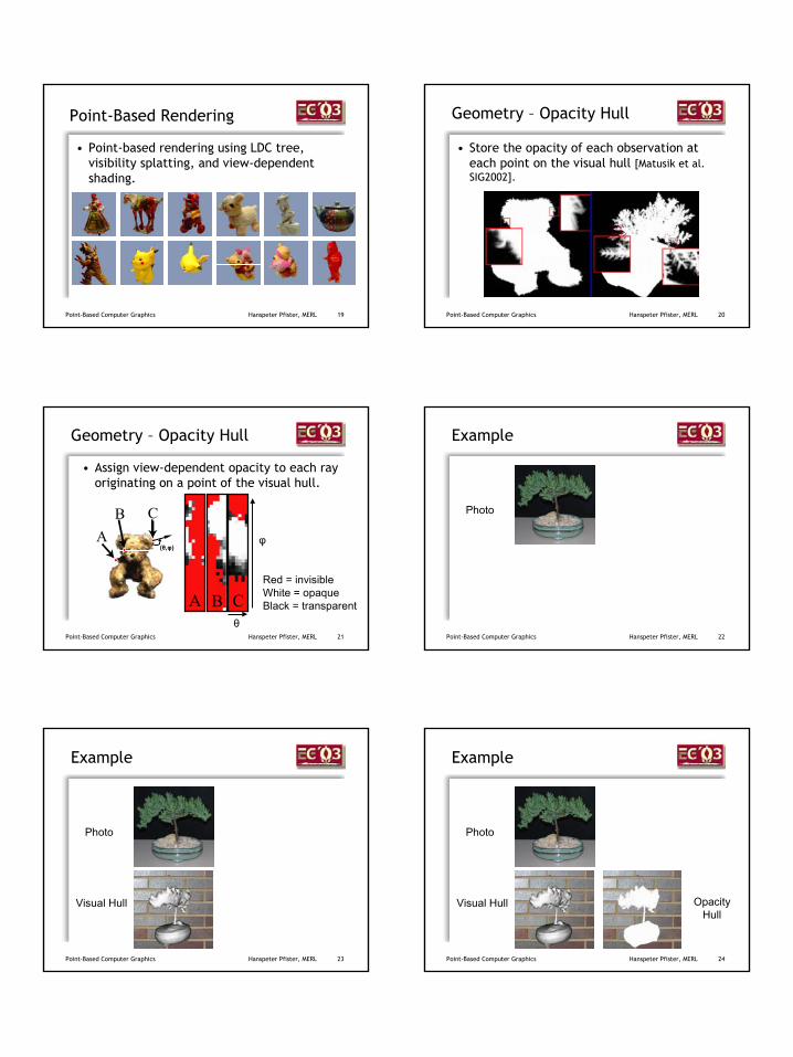
Geometry Example
Point-Based Computer Graphics Hanspeter Pfister, MERL 15
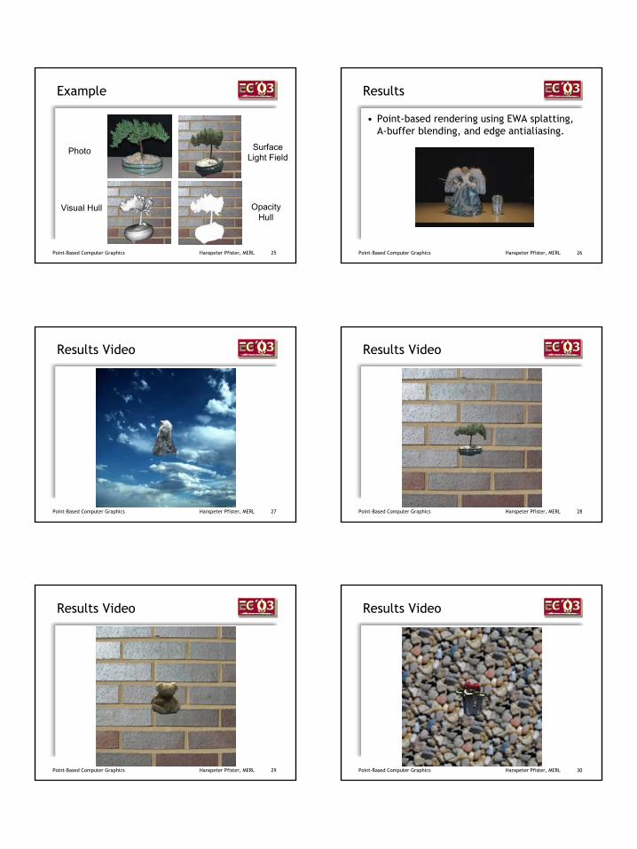
Approximate Geometry
• The approximate visual hull is augmented by radiance data to render concavities, reflections, and transparency.
Point-Based Computer Graphics Hanspeter Pfister, MERL 16
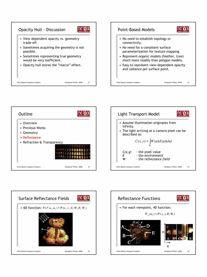
Surface Light Fields
• A surface light field is a function that assigns a color to each ray originating on a surface. [Wood et al., 2000]
Point-Based Computer Graphics Hanspeter Pfister, MERL 17
Shading Algorithm
• A view-dependent strategy.
Point-Based Computer Graphics Hanspeter Pfister, MERL 18
Color Blending
• Blend colors based on angle between virtual camera and stored colors.
• Unstructured Lumigraph Rendering[Buehler et al., SIGGRAPH 2001]
• View-Dependent Texture Mapping[Debevec, EGRW 98]
Point-Based Computer Graphics Hanspeter Pfister, MERL 19
Point-Based Rendering
• Point-based rendering using LDC tree, visibility splatting, and view-dependent shading.
Point-Based Computer Graphics Hanspeter Pfister, MERL 20
Geometry – Opacity Hull
• Store the opacity of each observation at each point on the visual hull [Matusik et al. SIG2002].
Point-Based Computer Graphics Hanspeter Pfister, MERL 21
Geometry – Opacity Hull
• Assign view-dependent opacity to each ray originating on a point of the visual hull.
Red = invisibleWhite = opaqueBlack = transparent
φAB C
A B C
(θ,φ)
θPoint-Based Computer Graphics Hanspeter Pfister, MERL 22
Example
Photo
Point-Based Computer Graphics Hanspeter Pfister, MERL 23
Example
Photo
Visual Hull
Point-Based Computer Graphics Hanspeter Pfister, MERL 24
Example
Photo
Visual Hull OpacityHull
Point-Based Computer Graphics Hanspeter Pfister, MERL 25
Example
Photo
Visual Hull OpacityHull
SurfaceLight Field
Point-Based Computer Graphics Hanspeter Pfister, MERL 26
Results
• Point-based rendering using EWA splatting, A-buffer blending, and edge antialiasing.
Point-Based Computer Graphics Hanspeter Pfister, MERL 27
Results Video
Point-Based Computer Graphics Hanspeter Pfister, MERL 28
Results Video
Point-Based Computer Graphics Hanspeter Pfister, MERL 29
Results Video
Point-Based Computer Graphics Hanspeter Pfister, MERL 30
Results Video
Point-Based Computer Graphics Hanspeter Pfister, MERL 31
Opacity Hull - Discussion
• View dependent opacity vs. geometry trade-off.
• Sometimes acquiring the geometry is not possible.
• Sometimes representing true geometry would be very inefficient.
• Opacity hull stores the “macro” effect.
Point-Based Computer Graphics Hanspeter Pfister, MERL 32
Point-Based Models
• No need to establish topology or connectivity.
• No need for a consistent surface parameterization for texture mapping.
• Represent organic models (feather, tree) much more readily than polygon models.
• Easy to represent view-dependent opacity and radiance per surface point.
Point-Based Computer Graphics Hanspeter Pfister, MERL 33
Outline
• Overview• Previous Works• Geometry
Reflectance• Refraction & Transparency
Point-Based Computer Graphics Hanspeter Pfister, MERL 34
Light Transport Model
• Assume illumination originates from infinity.
• The light arriving at a camera pixel can be described as:
C(x,y) - the pixel valueE - the environmentW - the reflectance field
ωωω dEWyxC )()(),( ∫Ω
=
Point-Based Computer Graphics Hanspeter Pfister, MERL 35
Surface Reflectance Fields
• 6D function:i
r
P
),;,;,(),,( rriirrri vuWPW ΦΦ= θθωω
i
Point-Based Computer Graphics Hanspeter Pfister, MERL 36
Reflectance Functions
• For each viewpoint, 4D function:
(θi,φi)
θi
φi
),;,()( iiixy yxWW Φ= θω
Point-Based Computer Graphics Hanspeter Pfister, MERL 37
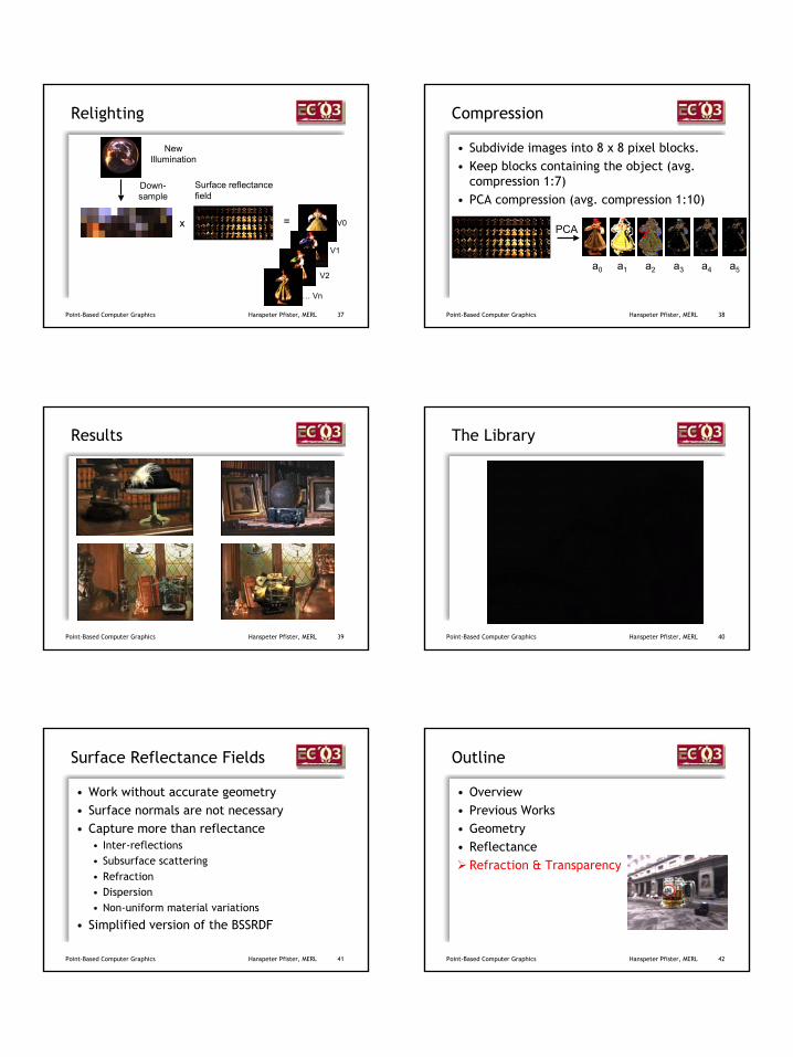
Relighting
x
Surface reflectance field
New Illumination
= V0
V1
V2
… Vn
Down-sample
Point-Based Computer Graphics Hanspeter Pfister, MERL 38
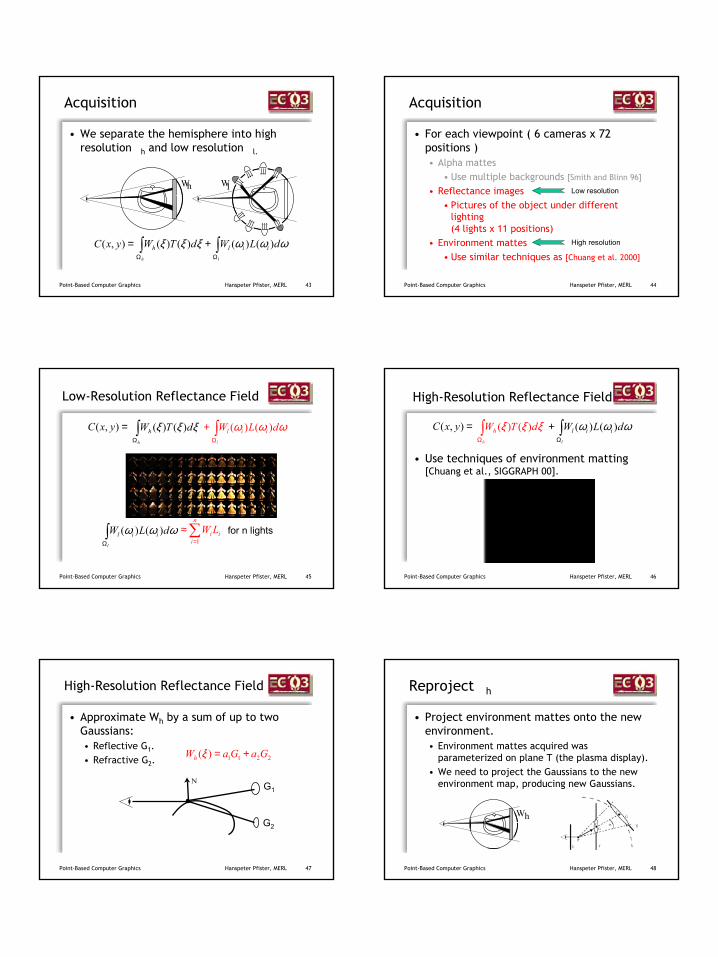
• Subdivide images into 8 x 8 pixel blocks.• Keep blocks containing the object (avg.
compression 1:7)• PCA compression (avg. compression 1:10)
Compression
PCA
a0 a1 a2 a3 a4 a5
Point-Based Computer Graphics Hanspeter Pfister, MERL 39
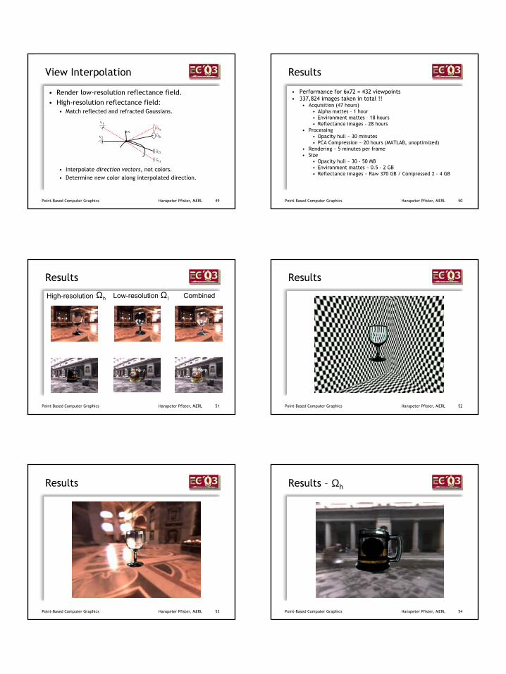
Results
Point-Based Computer Graphics Hanspeter Pfister, MERL 40
The Library
Point-Based Computer Graphics Hanspeter Pfister, MERL 41
Surface Reflectance Fields
• Work without accurate geometry• Surface normals are not necessary• Capture more than reflectance
• Inter-reflections• Subsurface scattering• Refraction• Dispersion• Non-uniform material variations
• Simplified version of the BSSRDF
Point-Based Computer Graphics Hanspeter Pfister, MERL 42
Outline
• Overview• Previous Works• Geometry• Reflectance
Refraction & Transparency
Point-Based Computer Graphics Hanspeter Pfister, MERL 43
Acquisition
• We separate the hemisphere into high resolution h and low resolution l.
ωωωξξξ dLWdTWyxC iilh
lh
)()()()(),( ∫∫ΩΩ
+=
Wh WlT
L()
Point-Based Computer Graphics Hanspeter Pfister, MERL 44
Acquisition
• For each viewpoint ( 6 cameras x 72 positions )• Alpha mattes
• Use multiple backgrounds [Smith and Blinn 96]
• Reflectance images• Pictures of the object under different
lighting (4 lights x 11 positions)
• Environment mattes• Use similar techniques as [Chuang et al. 2000]
Low resolution
High resolution
Point-Based Computer Graphics Hanspeter Pfister, MERL 45
Low-Resolution Reflectance Field
ωωω dLW iil
l
)()(∫Ω
∑=
≈n
iiiLW
1for n lights
ξξξ dTWh
h )()(∫Ω
=),( yxC ωωω dLW iil
l
)()(∫Ω
+
Point-Based Computer Graphics Hanspeter Pfister, MERL 46
High-Resolution Reflectance Field
• Use techniques of environment matting [Chuang et al., SIGGRAPH 00].
ξξξ dTWh
h )()(∫Ω
=),( yxC ωωω dLW iil
l
)()(∫Ω
+
Point-Based Computer Graphics Hanspeter Pfister, MERL 47
High-Resolution Reflectance Field
• Approximate Wh by a sum of up to twoGaussians:• Reflective G1.• Refractive G2.
N G1
G2
2211)( GaGaWh +=ξ
Point-Based Computer Graphics Hanspeter Pfister, MERL 48
Reproject h
• Project environment mattes onto the new environment.• Environment mattes acquired was
parameterized on plane T (the plasma display).• We need to project the Gaussians to the new
environment map, producing new Gaussians.
WhT
Point-Based Computer Graphics Hanspeter Pfister, MERL 49
View Interpolation
• Render low-resolution reflectance field.• High-resolution reflectance field:
• Match reflected and refracted Gaussians.
• Interpolate direction vectors, not colors.• Determine new color along interpolated direction.
V1
V2
G1r
G1t
G2r
G2t
N ~
~
~
~
Point-Based Computer Graphics Hanspeter Pfister, MERL 50
Results
• Performance for 6x72 = 432 viewpoints• 337,824 images taken in total !!
• Acquisition (47 hours)• Alpha mattes – 1 hour• Environment mattes – 18 hours• Reflectance images – 28 hours
• Processing• Opacity hull ~ 30 minutes• PCA Compression ~ 20 hours (MATLAB, unoptimized)
• Rendering ~ 5 minutes per frame• Size
• Opacity hull ~ 30 - 50 MB• Environment mattes ~ 0.5 - 2 GB• Reflectance images ~ Raw 370 GB / Compressed 2 - 4 GB
Point-Based Computer Graphics Hanspeter Pfister, MERL 51
Results
hΩHigh-resolution lΩLow-resolution Combined
Point-Based Computer Graphics Hanspeter Pfister, MERL 52
Results
Point-Based Computer Graphics Hanspeter Pfister, MERL 53
Results
Point-Based Computer Graphics Hanspeter Pfister, MERL 54
Results – Ωh
Point-Based Computer Graphics Hanspeter Pfister, MERL 55
Results – Ωl
Point-Based Computer Graphics Hanspeter Pfister, MERL 56
Results – Combined
Point-Based Computer Graphics Hanspeter Pfister, MERL 57
Results
Point-Based Computer Graphics Hanspeter Pfister, MERL 58
Results
Point-Based Computer Graphics Hanspeter Pfister, MERL 59
Conclusions
• Data driven modeling is able to capture and render any type of object.
• Opacity hulls provide realistic 3D graphics models.
• Our models can be seamlessly inserted into new environments.
• Point-based rendering offers high image-quality for display of acquired models.
Point-Based Computer Graphics Hanspeter Pfister, MERL 60
Future Directions
• Real-time rendering • Done! [Vlasic et al., I3D 2003]
• Better environment matting• More than two Gaussians
• Better compression• MPEG-4 / JPEG 2000

Point-Based Computer Graphics Hanspeter Pfister, MERL 61
Acknowledgements
• Colleagues:• MIT: Chris Buehler, Tom Buehler• MERL: Bill Yerazunis, Darren Leigh, Michael
Stern
• Thanks to:• David Tames, Jennifer Roderick Pfister
• NSF grants CCR-9975859 and EIA-9802220• Papers available at:
http://www.merl.com/people/pfister/
1
Point-Based Computer Graphics
Marc Alexa, Carsten Dachsbacher, Markus Gross, Mark Pauly,
Hanspeter Pfister, Marc Stamminger, Matthias Zwicker
2
Point-based Surface Reps
• Marc Alexa• Discrete Geometric Modeling Group• Darmstadt University of Technology• [email protected]
3
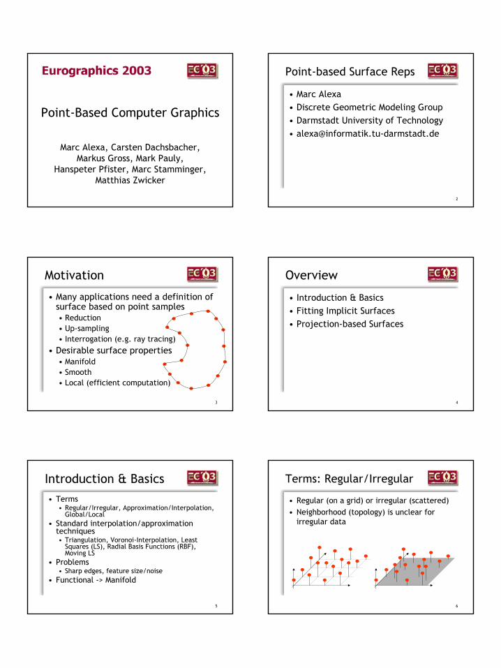
Motivation
• Many applications need a definition of surface based on point samples• Reduction• Up-sampling• Interrogation (e.g. ray tracing)
• Desirable surface properties• Manifold• Smooth• Local (efficient computation)
4
Overview
• Introduction & Basics• Fitting Implicit Surfaces• Projection-based Surfaces
5
Introduction & Basics• Terms
• Regular/Irregular, Approximation/Interpolation, Global/Local
• Standard interpolation/approximation techniques• Triangulation, Voronoi-Interpolation, Least
Squares (LS), Radial Basis Functions (RBF), Moving LS
• Problems• Sharp edges, feature size/noise
• Functional -> Manifold
6
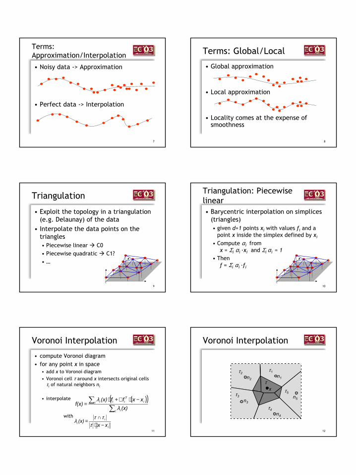
• Regular (on a grid) or irregular (scattered)• Neighborhood (topology) is unclear for
irregular data
Terms: Regular/Irregular
2
7
Terms: Approximation/Interpolation
• Noisy data -> Approximation
• Perfect data -> Interpolation
8
Terms: Global/Local
• Global approximation
• Local approximation
• Locality comes at the expense of smoothness
9
Triangulation
• Exploit the topology in a triangulation (e.g. Delaunay) of the data
• Interpolate the data points on the triangles• Piecewise linear C0• Piecewise quadratic C1?• …
10
• Barycentric interpolation on simplices(triangles)• given d+1 points xi with values fi and a
point x inside the simplex defined by xi
• Compute αi fromx = Σi αi ·xi and Σi αi = 1
• Thenf = Σi αi ·fi
Triangulation: Piecewise linear
11
Voronoi Interpolation
• compute Voronoi diagram• for any point x in space
• add x to Voronoi diagram• Voronoi cell τ around x intersects original cells
τi of natural neighbors ni
• interpolate
with
( )( )∑
∑ −⋅∇+⋅=
i i
i iTiii
(x)xxff(x)
f(x)λ
λ
i
ii xx(x)
−⋅∩
=τ
ττλ
12
Voronoi Interpolation
n1
x
τ1n2
τ2
n3τ3
n4τ4
n5τ5
τ
3
13
Properties of Voronoi Interpolation:• linear Precision• local• for d = 1 f(x) piecewise cubic• f(x)∈ C1 on domain• f(x,x1,...,xn ) is continuous in xi
Voronoi Interpolation
14
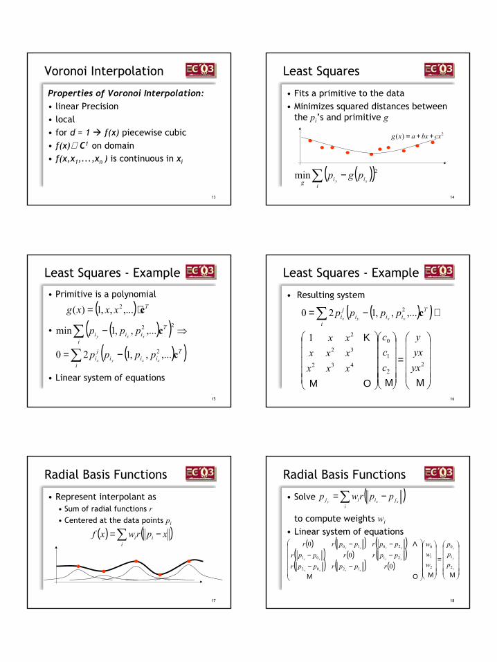
Least Squares
• Fits a primitive to the data• Minimizes squared distances between
the pi’s and primitive g
( )( )∑ −i
iig xypgp 2min
2)( cxbxaxg ++=
15
Least Squares - Example
• Primitive is a polynomial
•
• Linear system of equations
( ) Txxxg c⋅= ,...,,1)( 2
( )( )( )( )∑
∑−=
⇒−
i
Tiii
ji
i
Tiii
xxyx
xxy
pppp
ppp
c
c
,...,,120
,...,,1min
2
22
16
Least Squares - Example
• Resulting system
( )( )
=
⇔−=∑
ΜΜΟΜ
Κ
22
1
0
432
32
2
2
1
,...,,120
yxyxy
ccc
xxxxxxxx
ppppi
Tiii
ji xxyx
c
17
Radial Basis Functions
• Represent interpolant as• Sum of radial functions r• Centered at the data points pi
( ) ( )∑ −=i
ii xprwxf
18
Radial Basis Functions
• Solve
to compute weights wi• Linear system of equations
( )∑ −=i
jiij xxypprwp
( ) ( ) ( )( ) ( ) ( )( ) ( ) ( )
=
−−−−−−
ΜΜΟΜ
Λ
y
y
y
xxxx
xxxx
xxxx
ppp
www
rpprpprpprrpprpprpprr
2
1
0
2
1
0
1202
2101
2010
00
0
4
19
Radial Basis Functions
• Solvability depends on radial function• Several choices assure solvability
• (thin plate spline)
• (Gaussian)• h is a data parameter• h reflects the feature size or anticipated
spacing among points
( ) dddr log2=
( ) 22 /hdedr −=
20
• Monomial, Lagrange, RBF share the same principle:• Choose basis of a function space• Find weight vector for base elements by
solving linear system defined by data points
• Compute values as linear combinations• Properties
• One costly preprocessing step• Simple evaluation of function in any point
Function Spaces!
21
• Problems• Many points lead to large linear systems• Evaluation requires global solutions
• Solutions• RBF with compact support
• Matrix is sparse• Still: solution depends on every data point,
though drop-off is exponential with distance
• Local approximation approaches
Function Spaces?
22
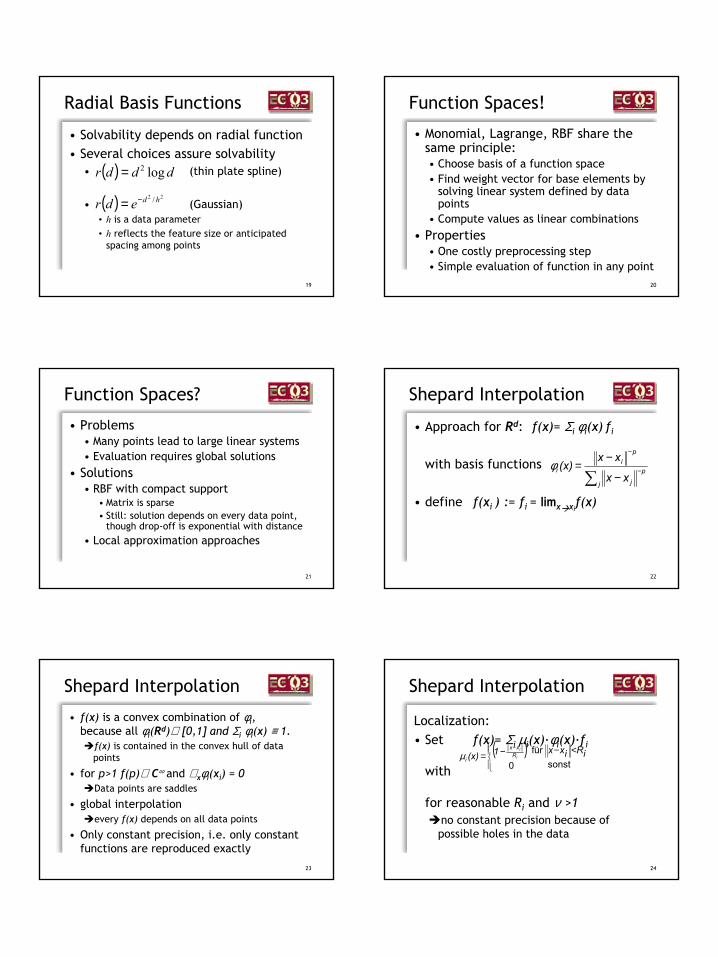
Shepard Interpolation
• Approach for Rd: f(x)= Σi φi(x) fi
with basis functions
• define f(xi ) := fi = limx xif(x)
∑−
−
−
−=
j
pj
pi
ixx
xx(x)φ
23
Shepard Interpolation
• f(x) is a convex combination of φi, because all φi(Rd)⊆ [0,1] and Σi φi(x) ≡ 1.
f(x) is contained in the convex hull of data points
• for p>1 f(p)∈ C∞ and ∇ xφi(xi) = 0Data points are saddles
• global interpolation every f(x) depends on all data points
• Only constant precision, i.e. only constant functions are reproduced exactly
24
Shepard Interpolation
Localization:• Set f(x)= Σi µi(x)·φi(x)·fi
with
for reasonable Ri and ν >1no constant precision because of possible holes in the data
( )
<−−=
−
sonstfür
0iRixx1(x) i
iRxx
i
ν
µ
5
25
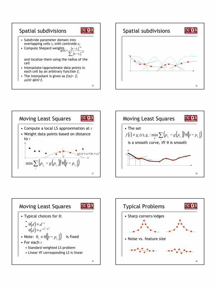
Spatial subdivisions
• Subdivide parameter domain into overlapping cells τi with centroids ci
• Compute Shepard weights
and localize them using the radius of the cell
• Interpolate/approximate data points in each cell by an arbitrary function fi
• The interpolant is given as f(x)= Σi µi(x)·φi(x)·fi
∑ −
−
−
−=
j
pj
pi
icx
cx(x)φ
26
Spatial subdivisions
27
Moving Least Squares
• Compute a local LS approximation at t• Weight data points based on distance
to t
( )( ) ( )xxy i
iii ptpgp −−∑ θmin 2
2)( cxbxaxg ++=t
28
Moving Least Squares
• The set
is a smooth curve, iff θ is smooth
( ) ( )( ) ( )xxy i
iiigtt ptpgpgtgtf −−= ∑ θmin:),( 2
29
Moving Least Squares
• Typical choices for θ:••
• Note: is fixed• For each t
• Standard weighted LS problem• Linear iff corresponding LS is linear
( )xii pt −= θθ
( ) 22 /θ hded −=( ) rdd −=θ
30
Typical Problems
• Sharp corners/edges
• Noise vs. feature size
6
31
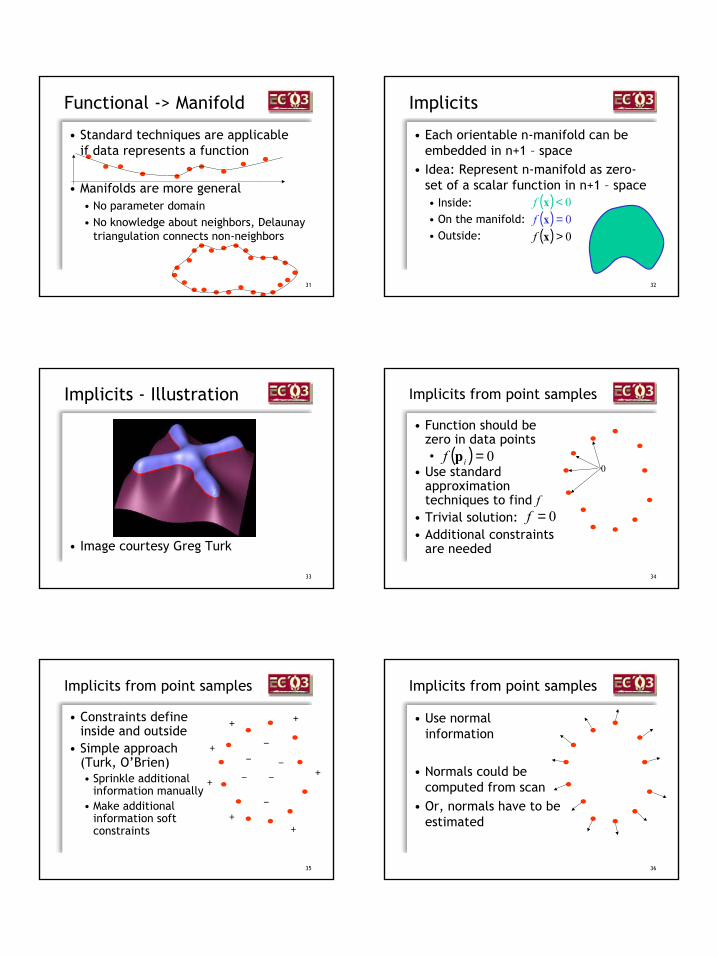
Functional -> Manifold
• Standard techniques are applicableif data represents a function
• Manifolds are more general• No parameter domain• No knowledge about neighbors, Delaunay
triangulation connects non-neighbors
32
Implicits
• Each orientable n-manifold can be embedded in n+1 – space
• Idea: Represent n-manifold as zero-set of a scalar function in n+1 – space • Inside:• On the manifold:• Outside:
( ) 0<xf( ) 0=xf( ) 0>xf
33
Implicits - Illustration
• Image courtesy Greg Turk
34
Implicits from point samples
• Function should be zero in data points•
• Use standard approximation techniques to find f
• Trivial solution:• Additional constraints
are needed
( ) 0=if p
0=f
0
35
Implicits from point samples
• Constraints define inside and outside
• Simple approach (Turk, O’Brien)• Sprinkle additional
information manually• Make additional
information soft constraints
−
−−
−
−
−
+
+
+
+
+
+
+
36
Implicits from point samples
• Use normal information
• Normals could be computed from scan
• Or, normals have to be estimated
7
37
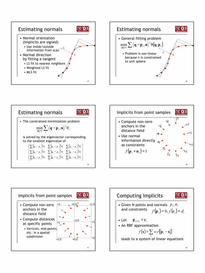
Estimating normals
• Normal orientation(Implicits are signed)• Use inside/outside
information from scan• Normal direction
by fitting a tangent• LS fit to nearest neighbors• Weighted LS fit• MLS fit
n
q
38
Estimating normals
• General fitting problem
• Problem is non-linearbecause n is constrainedto unit sphere
nq
( )∑ −= i
ii pqnpqn
,θ,min 2
1
39
Estimating normals
• The constrained minimization problem
is solved by the eigenvector corresponding to the smallest eigenvalue of
∑ −= i
ii θ,min 2
1npq
n
( ) ( ) ( )( ) ( ) ( )( ) ( ) ( )
−−−
−−−
−−−
∑∑∑∑∑∑∑∑∑
iiiz
iiiz
iiiz
iiiy
iiiy
iiiy
iiix
iiix
iiix
zyx
zyx
zyx
pqpqpq
pqpqpq
pqpqpq
θθθ
θθθ
θθθ
222
222
222
40
Implicits from point samples
• Compute non-zero anchors in the distance field
• Use normal information directly as constraints
+1
+1
+1
+1
+1
+1
+1+1
+1
+1
+1 +1
( ) 1=+ iif np
41
Implicits from point samples
• Compute non-zero anchors in the distance field
• Compute distances at specific points• Vertices, mid-points,
etc. in a spatial subdivision
−2.5
+0.5
+1 +1
+0.5+2.5 +2
+2 +1.5
42
Computing Implicits
• Given N points and normals and constraints
• Let • An RBF approximation
leads to a system of linear equations
( ) ( ) iii dff == cp ,0
iNi cp =+
( ) ( )∑ −=i
iirwf xpx
ii np ,
8
43
Computing Implicits
• Practical problems: N > 10000• Matrix solution becomes difficult• Two solutions
• Sparse matrices allow iterative solution• Smaller number of RBFs
44
Computing Implicits
• Sparse matrices
• Needed:
• Compactly supported RBFs
( ) ( ) ( )( ) ( ) ( )( ) ( ) ( )
−−−−−−
ΟΜ
Λ
00
0
120
2101
2010
rpprpprpprrpprpprpprr
0)(',0)( ==→> crdrcd
cc
45
Computing Implicits
• Smaller number of RBFs• Greedy approach (Carr et al.)
• Start with random small subset• Add RBFs where approximation quality is
not sufficient
46
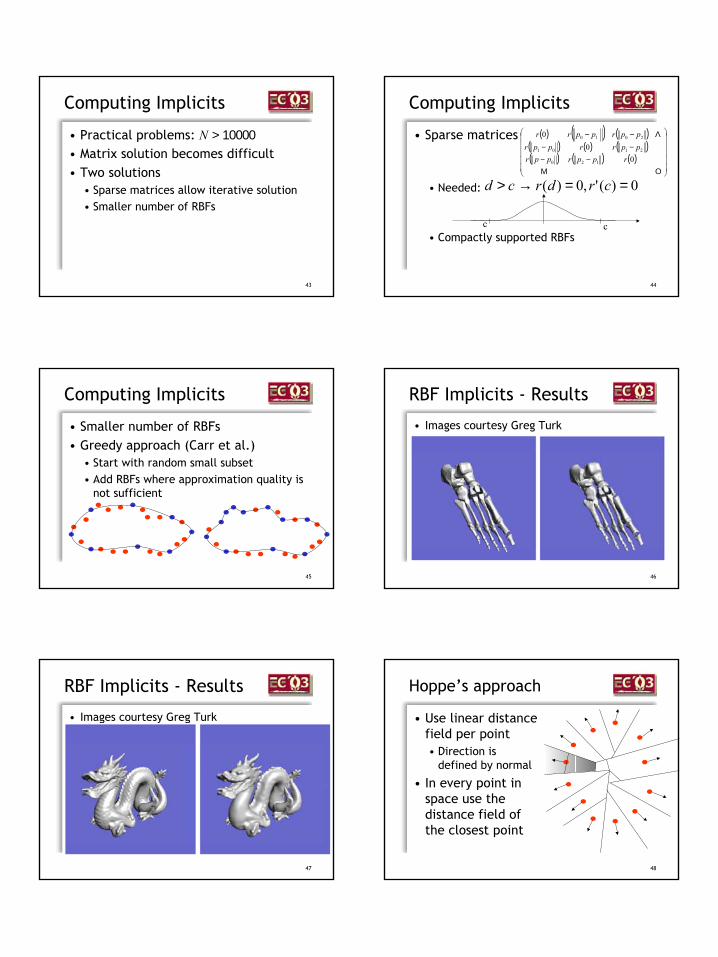
RBF Implicits - Results
• Images courtesy Greg Turk
47
RBF Implicits - Results
• Images courtesy Greg Turk
48
Hoppe’s approach
• Use linear distancefield per point• Direction is
defined by normal
• In every point inspace use thedistance field ofthe closest point
9
49
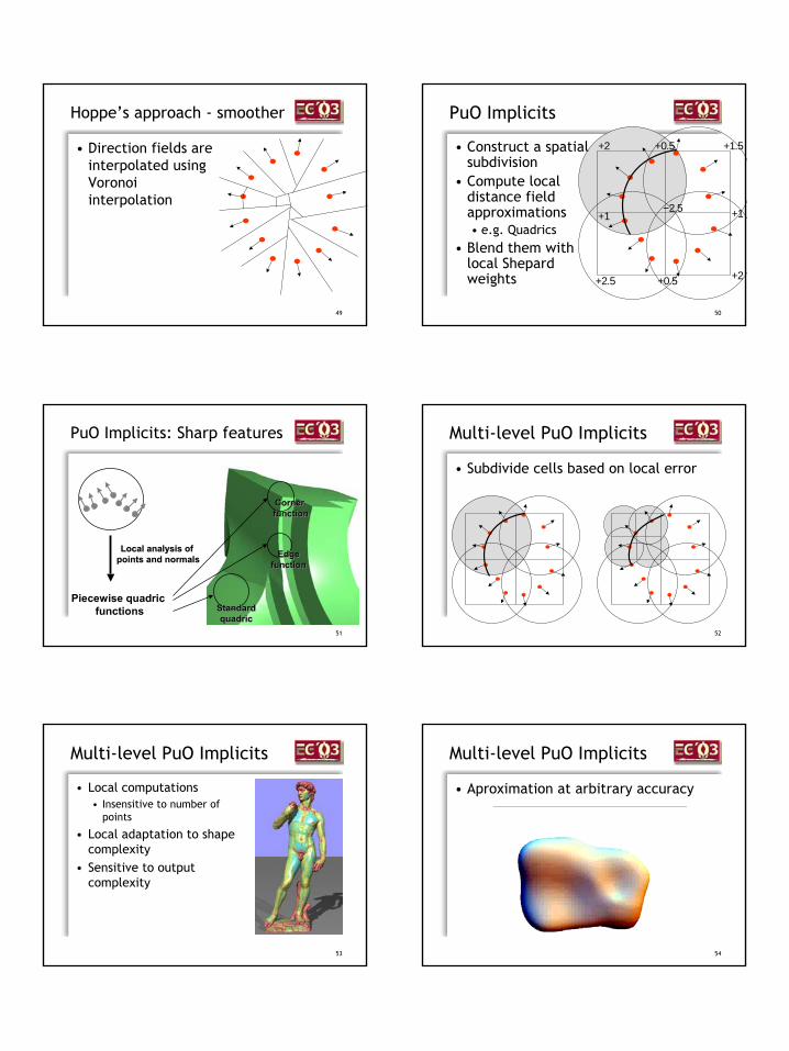
Hoppe’s approach - smoother
• Direction fields are interpolated using Voronoi interpolation
50
PuO Implicits
• Construct a spatial subdivision
• Compute local distance field approximations• e.g. Quadrics
• Blend them withlocal Shepard weights
−2.5
+0.5
+1 +1
+0.5+2.5 +2
+2 +1.5
51
CornerCornerfunctionfunction
Edge Edge functionfunction
Standard Standard quadricquadric
Piecewise quadric functions
Local analysis of Local analysis of points andpoints and normalsnormals
PuO Implicits: Sharp features
52
Multi-level PuO Implicits
• Subdivide cells based on local error
53
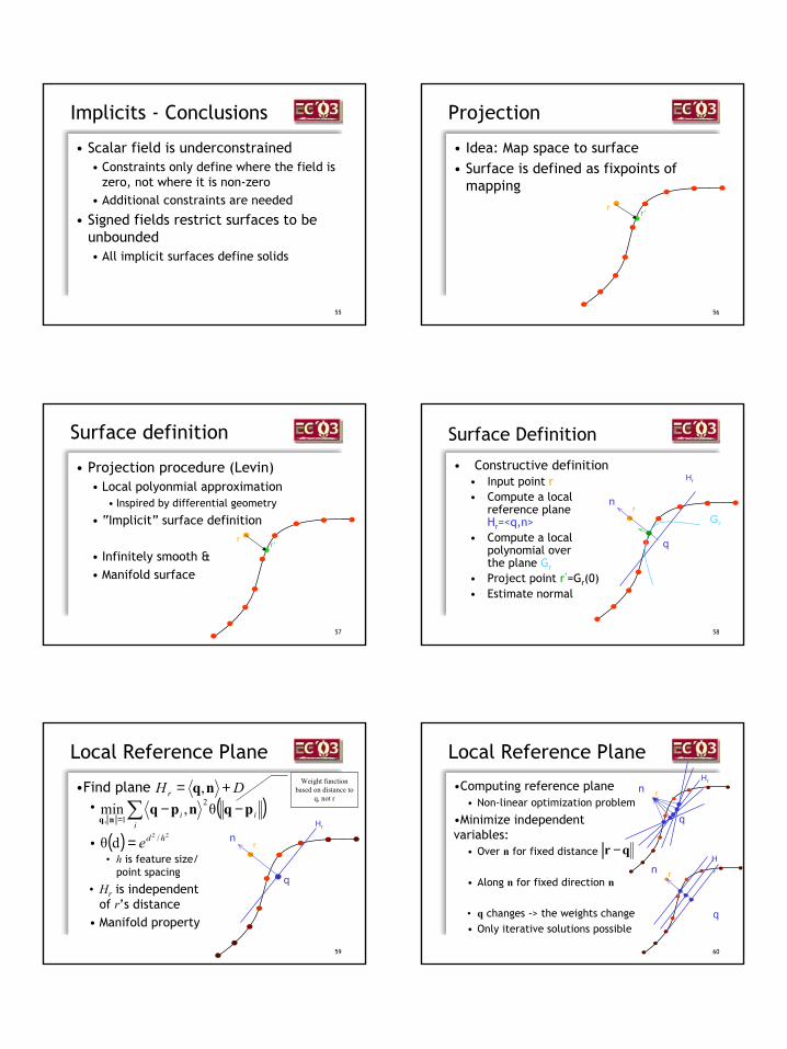
Multi-level PuO Implicits
• Local computations• Insensitive to number of
points
• Local adaptation to shape complexity
• Sensitive to output complexity
54
Multi-level PuO Implicits
• Aproximation at arbitrary accuracy
10
55
Implicits - Conclusions
• Scalar field is underconstrained• Constraints only define where the field is
zero, not where it is non-zero• Additional constraints are needed
• Signed fields restrict surfaces to be unbounded• All implicit surfaces define solids
56
Projection
• Idea: Map space to surface• Surface is defined as fixpoints of
mappingr
r’
57
Surface definition
• Projection procedure (Levin)• Local polyonmial approximation
• Inspired by differential geometry
• “Implicit” surface definition
• Infinitely smooth &• Manifold surface
rr’
58
Surface Definition
• Constructive definition• Input point r• Compute a local
reference planeHr=<q,n>
• Compute a localpolynomial overthe plane Gr
• Project point r’=Gr(0)• Estimate normal
rGr
Hr
q
n
59
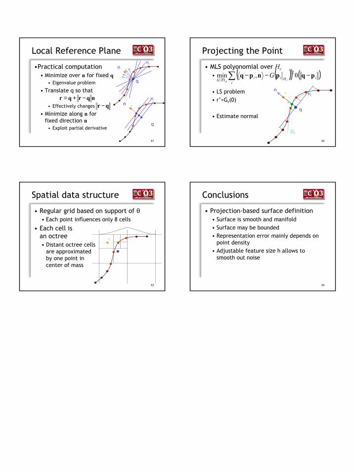
Local Reference Plane
•Find plane•
•• h is feature size/
point spacing
• Hr is independentof r’s distance
• Manifold property
r
Hr
q
n
Weight function based on distance to
q, not rDHr += nq,
( )∑ −−= i
ii pqnpqnq
θ,min 2
1,
( ) 22 /dθ hde=
60
Local Reference Plane
•Computing reference plane• Non-linear optimization problem
•Minimize independent variables:
• Over n for fixed distance
• Along n for fixed direction n
• q changes -> the weights change• Only iterative solutions possible
r
Hr
q
n
r
Hr
q
n
qr −
11
61
Local Reference Plane
•Practical computation• Minimize over n for fixed q
• Eigenvalue problem
• Translate q so that
• Effectively changes
• Minimize along n forfixed direction n
• Exploit partial derivative
r
Hr
q
n
r
Hr
q
nnqrqr −+=
qr −
62
Projecting the Point
• MLS polyonomial over Hr•
• LS problem• r’=Gr(0)
• Estimate normal
r
Gr
Hr
q
n
( )( ) ( )∑ −−−Π∈ i
iHiiG rd
G pqpnpq θ,min 2
63
Spatial data structure
• Regular grid based on support of θ• Each point influences only 8 cells
• Each cell isan octree• Distant octree cells
are approximatedby one point incenter of mass
r
64
Conclusions
• Projection-based surface definition• Surface is smooth and manifold• Surface may be bounded• Representation error mainly depends on
point density• Adjustable feature size h allows to
smooth out noise
1
Point-Based Rendering
Matthias ZwickerComputer Graphics Lab
ETH Zürich
2
Point-Based Rendering
• Introduction and motivation• Surface elements• Rendering• Antialiasing• Hardware Acceleration• Conclusions
3
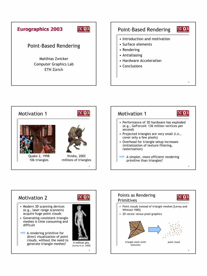
Motivation 1
Quake 2, 199810k triangles
Nvidia, 2002 millions of triangles
4
Motivation 1
• Performance of 3D hardware has exploded(e.g., GeForce4: 136 million vertices per second)
• Projected triangles are very small (i.e., cover only a few pixels)
• Overhead for triangle setup increases(initialization of texture filtering, rasterization)
A simpler, more efficient renderingprimitive than triangles?
5
Motivation 2
• Modern 3D scanning devices(e.g., laser range scanners) acquire huge point clouds
• Generating consistent triangle meshes is time consuming and difficult
A rendering primitive fordirect visualization of pointclouds, without the need togenerate triangle meshes? 4 million pts.
[Levoy et al. 2000]
6
Points as RenderingPrimitives• Point clouds instead of triangle meshes [Levoy and
Whitted 1985]• 2D vector versus pixel graphics
triangle mesh (with textures)
point cloud
2
7
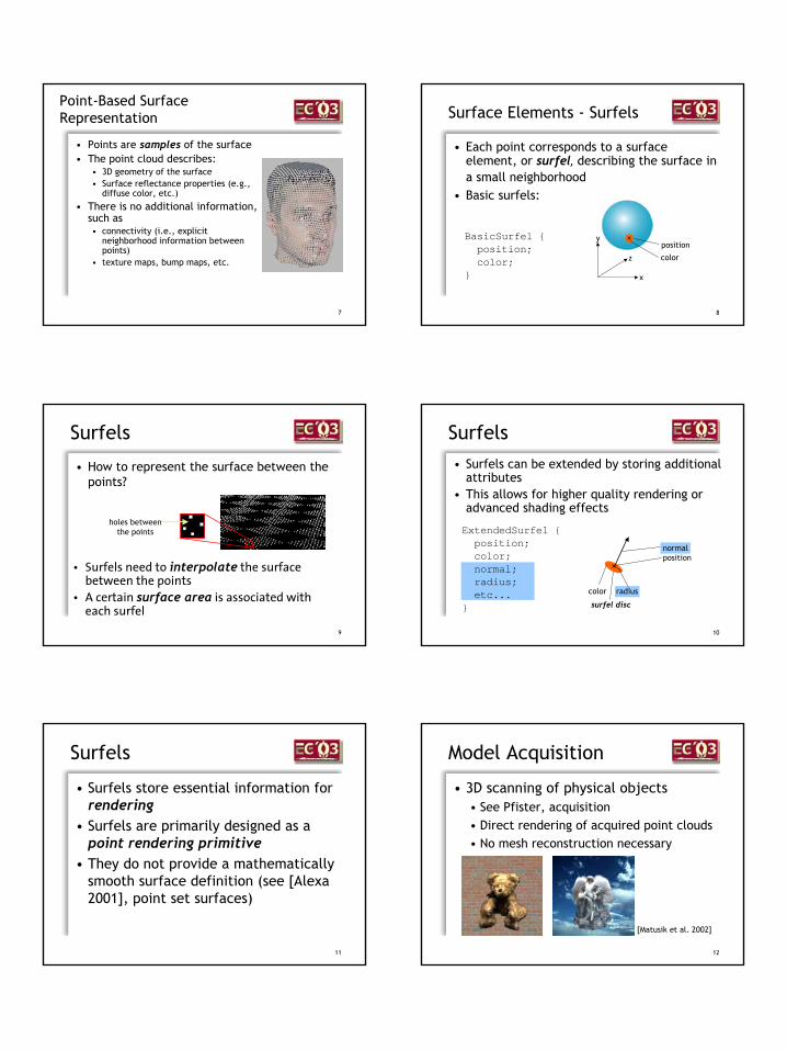
Point-Based Surface Representation
• Points are samples of the surface• The point cloud describes:
• 3D geometry of the surface• Surface reflectance properties (e.g.,
diffuse color, etc.)
• There is no additional information, such as• connectivity (i.e., explicit
neighborhood information between points)
• texture maps, bump maps, etc.
8
Surface Elements - Surfels
• Each point corresponds to a surface element, or surfel, describing the surface in a small neighborhood
• Basic surfels:
BasicSurfel position;color;
position
color
x
y
z
9
Surfels
• How to represent the surface between the points?
• Surfels need to interpolate the surface between the points
• A certain surface area is associated with each surfel
holes between the points
10
ExtendedSurfel position;color; normal;radius;etc...
Surfels• Surfels can be extended by storing additional
attributes• This allows for higher quality rendering or
advanced shading effects
normalposition
color radius
surfel disc
11
Surfels
• Surfels store essential information for rendering
• Surfels are primarily designed as a point rendering primitive
• They do not provide a mathematically smooth surface definition (see [Alexa 2001], point set surfaces)
12
Model Acquisition
• 3D scanning of physical objects• See Pfister, acquisition• Direct rendering of acquired point clouds• No mesh reconstruction necessary
[Matusik et al. 2002]
3
13
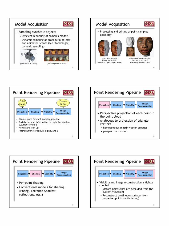
Model Acquisition
• Sampling synthetic objects• Efficient rendering of complex models• Dynamic sampling of procedural objects
and animated scenes (see Stamminger, dynamic sampling)
[Zwicker et al. 2001] [Stamminger et al. 2001]
14
Model Acquisition
• Processing and editing of point-sampled geometry
point-based surface editing[Zwicker et al. 2002]
(see Pauly, Pointshop3D)
spectral processing[Pauly, Gross 2002]
(see Gross, spectral processing)
15
Visibility ImageReconstructionShadingProjection
• Simple, pure forward mapping pipeline• Surfels carry all information through the pipeline
(„surfel stream“)• No texture look-ups• Framebuffer stores RGB, alpha, and Z
PointCloud
Frame-buffer
Point Rendering Pipeline
16
• Perspective projection of each point in the point cloud
• Analogous to projection of triangle vertices• homogeneous matrix-vector product• perspective division
Point Rendering Pipeline
Visibility ImageReconstructionShadingProjection
17
• Per-point shading• Conventional models for shading
(Phong, Torrance-Sparrow, reflections, etc.)
Point Rendering Pipeline
Visibility ImageReconstructionShadingProjection
18
• Visibility and image reconstruction is tightly coupled• Discard points that are occluded from the
current viewpoint• Reconstruct continuous surfaces from
projected points (antialiasing)
Point Rendering Pipeline
Visibility ImageReconstructionShadingProjection
4
19
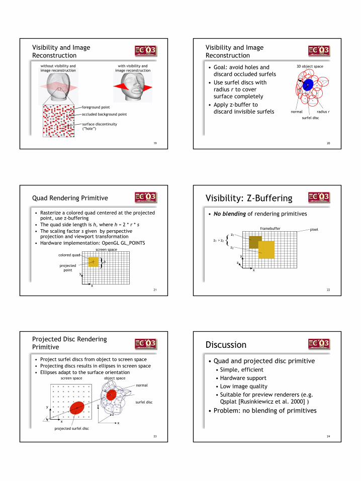
Visibility and Image Reconstruction
with visibility and image reconstruction
without visibility and image reconstruction
foreground point
occluded background point
surface discontinuity (“hole”)
20
• Goal: avoid holes and discard occluded surfels
• Use surfel discs with radius r to cover surface completely
• Apply z-buffer to discard invisible surfels radius r
3D object space
surfel disc
normal
Visibility and Image Reconstruction
21
• Rasterize a colored quad centered at the projectedpoint, use z-buffering
• The quad side length is h, where h = 2 * r * s• The scaling factor s given by perspective
projection and viewport transformation• Hardware implementation: OpenGL GL_POINTS
x
y
screen space
h
colored quad
projected point
Quad Rendering Primitive
22
Visibility: Z-Buffering
• No blending of rendering primitives
y
framebuffer
x
z2
z1
z
z1 > z2pixel
23
• Project surfel discs from object to screen space• Projecting discs results in ellipses in screen space• Ellipses adapt to the surface orientation
screen space object space
x
y y
z
x
normal
surfel disc
projected surfel disc
Projected Disc Rendering Primitive
24
Discussion
• Quad and projected disc primitive• Simple, efficient• Hardware support• Low image quality• Suitable for preview renderers (e.g.
Qsplat [Rusinkiewicz et al. 2000] )
• Problem: no blending of primitives
5
25
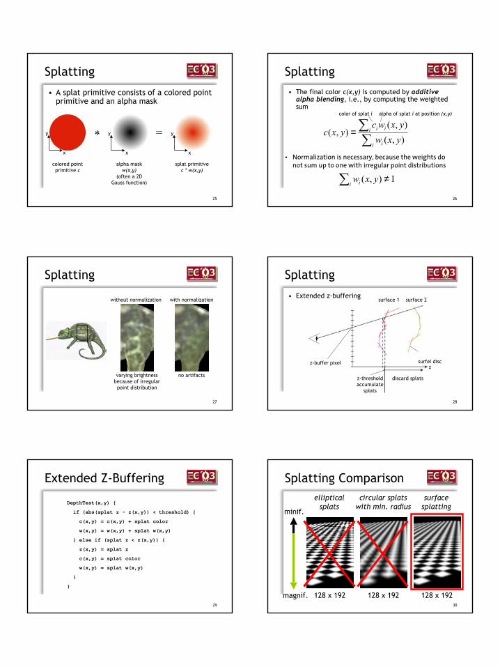
Splatting
• A splat primitive consists of a colored point primitive and an alpha mask
colored point primitive c
alpha mask w(x,y)
(often a 2D Gauss function)
splat primitivec * w(x,y)
y
x
y
x
y
x
* =
26
∑∑=
i i
i ii
yxwyxwc
yxc),(),(
),(
Splatting
• Normalization is necessary, because the weights do not sum up to one with irregular point distributions
• The final color c(x,y) is computed by additive alpha blending, i.e., by computing the weighted sum
color of splat i alpha of splat i at position (x,y)
1),( ≠∑i i yxw
27
Splatting
varying brightness because of irregular
point distribution
without normalization with normalization
no artifacts
28
Splatting
• Extended z-buffering
zz-buffer pixel surfel disc
surface 2surface 1
z-thresholdaccumulate
splats
discard splats
29
Extended Z-Buffering
DepthTest(x,y)
if (abs(splat z – z(x,y)) < threshold)
c(x,y) = c(x,y) + splat color
w(x,y) = w(x,y) + splat w(x,y)
else if (splat z < z(x,y))
z(x,y) = splat z
c(x,y) = splat color
w(x,y) = splat w(x,y)
30
Splatting Comparison
minif.
magnif. 128 x 192
ellipticalsplats
128 x 192
circular splatswith min. radius
128 x 192
surfacesplatting
6
31
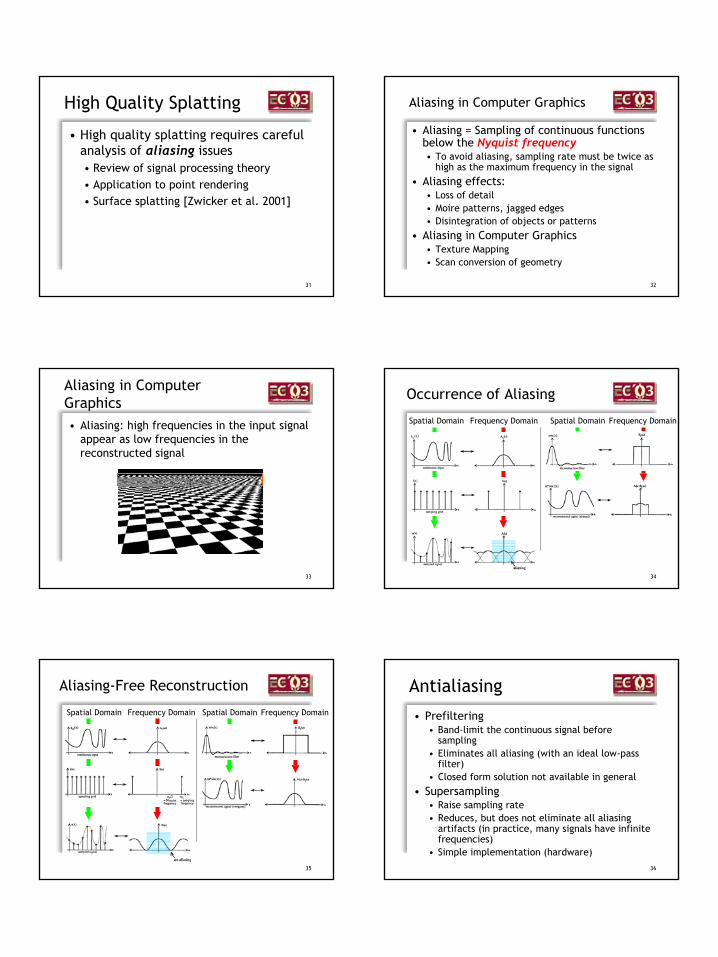
High Quality Splatting
• High quality splatting requires careful analysis of aliasing issues• Review of signal processing theory• Application to point rendering• Surface splatting [Zwicker et al. 2001]
32
Aliasing in Computer Graphics
• Aliasing = Sampling of continuous functions below the Nyquist frequency• To avoid aliasing, sampling rate must be twice as
high as the maximum frequency in the signal
• Aliasing effects:• Loss of detail• Moire patterns, jagged edges• Disintegration of objects or patterns
• Aliasing in Computer Graphics• Texture Mapping• Scan conversion of geometry
33
Aliasing in Computer Graphics• Aliasing: high frequencies in the input signal
appear as low frequencies in the reconstructed signal
34
Occurrence of Aliasing
Spatial Domain Frequency Domain Spatial Domain Frequency Domain
35
Aliasing-Free Reconstruction
Spatial Domain Frequency Domain Spatial Domain Frequency Domain
36
Antialiasing
• Prefiltering• Band-limit the continuous signal before
sampling• Eliminates all aliasing (with an ideal low-pass
filter)• Closed form solution not available in general
• Supersampling• Raise sampling rate• Reduces, but does not eliminate all aliasing
artifacts (in practice, many signals have infinite frequencies)
• Simple implementation (hardware)
7
37
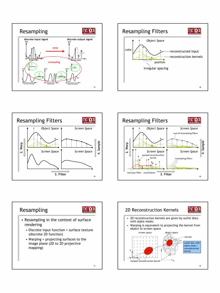
Resampling
1.
warp
2. 3.
4.
discrete input signal discrete output signal
resampling
38
Resampling Filters
Object Space
reconstruction kernels
reconstructed input
position
color
irregular spacing
39
Resampling FiltersObject Space
3. Filter
Screen Space2. W
arp
Screen Space
4. S
ampl
e
Screen Space
40
Resampling FiltersObject Space
3. Filter
Screen Space2. W
arp
Screen Space
4. S
ampl
e
Screen Space
low-pass filter convolution
resampling filters
sum of resampling filters
warped reconstruction kernel
41
Resampling
• Resampling in the context of surface rendering• Discrete input function = surface texture
(discrete 2D function)• Warping = projecting surfaces to the
image plane (2D to 2D projective mapping)
42
2D Reconstruction Kernels
• 2D reconstruction kernels are given by surfel discs with alpha masks
• Warping is equivalent to projecting the kernel from object to screen space
screen space object space
x
y y
z
x
normal
surfel disc with alpha mask = reconstruction kernel
warped reconstruction kernel
8
43
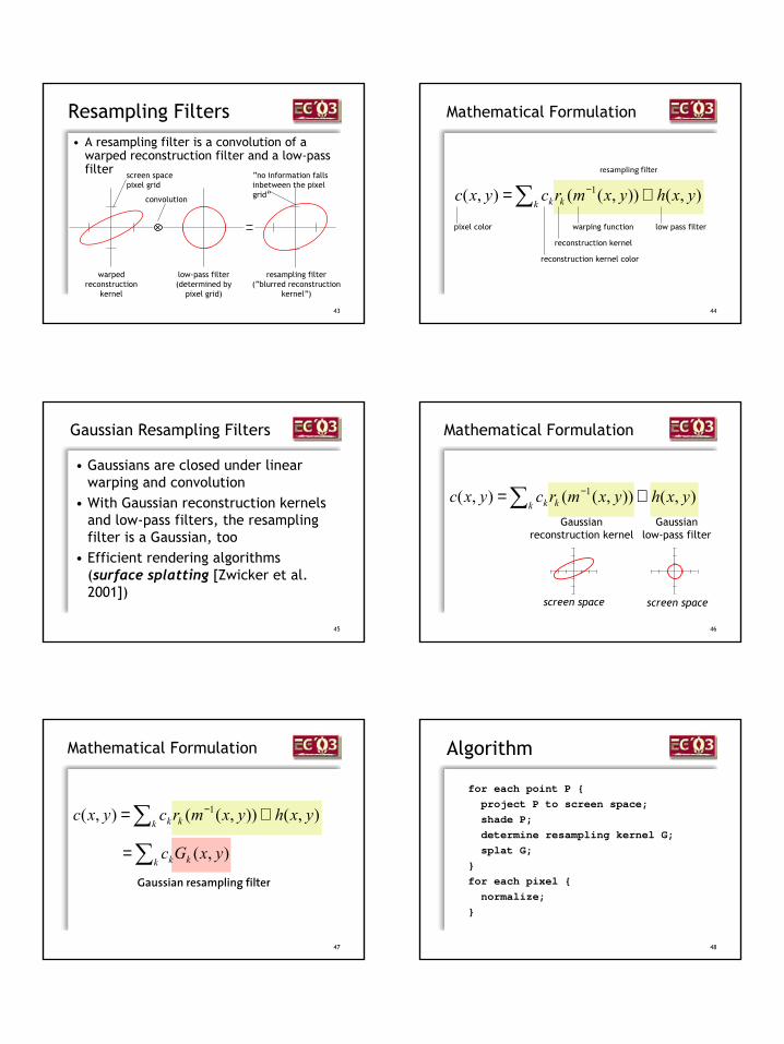
Resampling Filters• A resampling filter is a convolution of a
warped reconstruction filter and a low-pass filter
warped reconstruction
kernel
low-pass filter (determined by
pixel grid)
resampling filter(“blurred reconstruction
kernel”)
screen space pixel grid
“no information falls inbetween the pixel grid”convolution
44
resampling filter
Mathematical Formulation
∑ ⊗= −k kk yxhyxmrcyxc ),()),((),( 1
pixel color
reconstruction kernel
warping function low pass filter
reconstruction kernel color
45
Gaussian Resampling Filters
• Gaussians are closed under linear warping and convolution
• With Gaussian reconstruction kernelsand low-pass filters, the resampling filter is a Gaussian, too
• Efficient rendering algorithms(surface splatting [Zwicker et al. 2001])
46
Mathematical Formulation
Gaussianreconstruction kernel
Gaussianlow-pass filter
∑ ⊗= −k kk yxhyxmrcyxc ),()),((),( 1
screen space screen space
47
Mathematical Formulation
∑ ⊗= −k kk yxhyxmrcyxc ),()),((),( 1
∑=k kk yxGc ),(
Gaussian resampling filter
48
Algorithm
for each point P
project P to screen space;
shade P;
determine resampling kernel G;
splat G;
for each pixel
normalize;
9
49
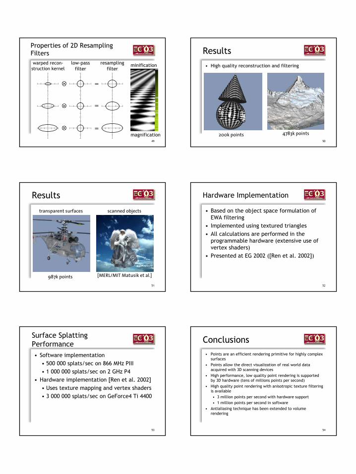
Properties of 2D ResamplingFilterswarped recon-
struction kernellow-pass
filterresampling
filterminification
magnification50
Results
• High quality reconstruction and filtering
200k points 4783k points
51
Results
987k points
transparent surfaces scanned objects
[MERL/MIT Matusik et al.]
52
Hardware Implementation
• Based on the object space formulation of EWA filtering
• Implemented using textured triangles• All calculations are performed in the
programmable hardware (extensive use of vertex shaders)
• Presented at EG 2002 ([Ren et al. 2002])
53
Surface Splatting Performance• Software implementation
• 500 000 splats/sec on 866 MHz PIII• 1 000 000 splats/sec on 2 GHz P4
• Hardware implementation [Ren et al. 2002]• Uses texture mapping and vertex shaders• 3 000 000 splats/sec on GeForce4 Ti 4400
54
Conclusions• Points are an efficient rendering primitive for highly complex
surfaces• Points allow the direct visualization of real world data
acquired with 3D scanning devices• High performance, low quality point rendering is supported
by 3D hardware (tens of millions points per second)• High quality point rendering with anisotropic texture filtering
is available • 3 million points per second with hardware support• 1 million points per second in software
• Antialiasing technique has been extended to volume rendering

10
55
Applications
• Direct visualization of point clouds• Real-time 3D reconstruction and rendering
for virtual reality applications• Hybrid point and polygon rendering systems• Rendering animated scenes• Interactive display of huge meshes• On the fly sampling and rendering of
procedural objects
56
Future Work
• Dedicated rendering hardware• Efficient approximations of exact EWA
splatting• Rendering architecture for on the fly
sampling and rendering
57
Acknowledgments
• Hanspeter Pfister, Jeroen van Baar(MERL, Cambridge MA)
• Markus Gross, Mark Pauly, CGL• Liu Ren
http://graphics.ethz.ch/surfelshttp://graphics.ethz.ch/pointshop3d
58
References• [Levoy and Whitted 1985] The use of points as a display primitive,
technical report, University of North Carolina at Chapel Hill, 1985• [Heckbert 1986] Fundamentals of texture mapping and image warping,
Master‘s Thesis, 1986• [Grossman and Dally 1998] Point sample rendering, Eurographics
workshop on rendering, 1998• [Levoy et al. 2000] The digital Michelangelo project, SIGGRAPH 2000• [Rusinkiewicz et al. 2000] Qsplat, SIGGRAPH 2000• [Pfister et al. 2000] Surfels: Surface elements as rendering primitives,
SIGGRAPH 2000• [Zwicker et al. 2001] Surface splatting, SIGGRAPH 2001• [Zwicker et al. 2002] EWA Splatting, to appear, IEEE TVCG 2002• [Ren et al. 2002] Object space EWA splatting: A hardware accelerated
approach to high quality point rendering, Eurographics 2002
1
Point-Based Computer Graphics
Marc Alexa, Carsten Dachsbacher, Markus Gross, Mark Pauly,
Hanspeter Pfister, Marc Stamminger, Matthias Zwicker
2
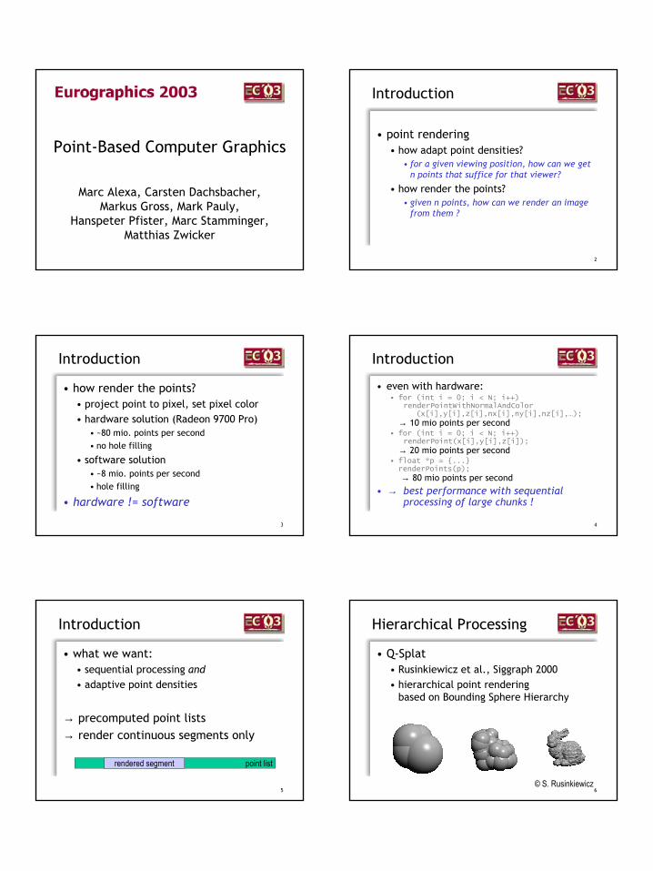
Introduction
• point rendering• how adapt point densities?
• for a given viewing position, how can we getn points that suffice for that viewer?
• how render the points?• given n points, how can we render an image
from them ?
3
Introduction
• how render the points?• project point to pixel, set pixel color• hardware solution (Radeon 9700 Pro)
• ~80 mio. points per second• no hole filling
• software solution• ~8 mio. points per second• hole filling
• hardware != software
4
Introduction
• even with hardware:• for (int i = 0; i < N; i++)
renderPointWithNormalAndColor(x[i],y[i],z[i],nx[i],ny[i],nz[i],…);
→ 10 mio points per second• for (int i = 0; i < N; i++)
renderPoint(x[i],y[i],z[i]);
→ 20 mio points per second• float *p = ...renderPoints(p);
→ 80 mio points per second
• → best performance with sequentialprocessing of large chunks !
5
Introduction
• what we want:• sequential processing and• adaptive point densities
→ precomputed point lists→ render continuous segments only
point listrendered segment
6
Hierarchical Processing
• Q-Splat• Rusinkiewicz et al., Siggraph 2000• hierarchical point rendering
based on Bounding Sphere Hierarchy
© S. Rusinkiewicz
2
7
Hierarchical Processing
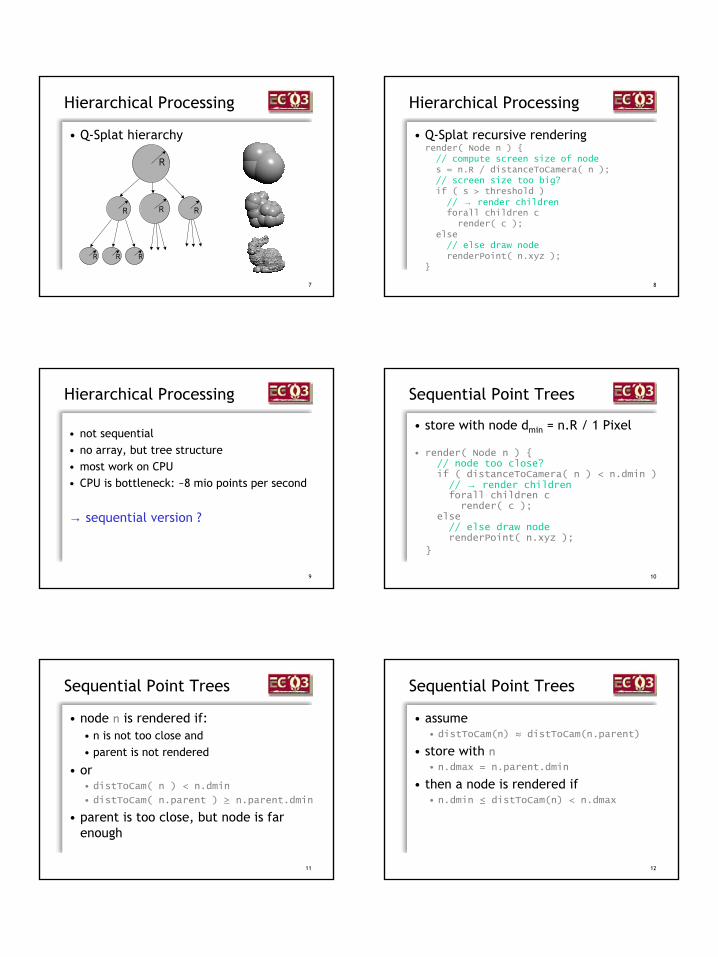
• Q-Splat hierarchy
R
R R R
R R R
8
Hierarchical Processing
• Q-Splat recursive renderingrender( Node n ) // compute screen size of nodes = n.R / distanceToCamera( n );// screen size too big?if ( s > threshold )// → render childrenforall children crender( c );
else// else draw noderenderPoint( n.xyz );
9
Hierarchical Processing
• not sequential• no array, but tree structure• most work on CPU• CPU is bottleneck: ~8 mio points per second
→ sequential version ?
10
Sequential Point Trees
• store with node dmin = n.R / 1 Pixel
• render( Node n ) // node too close?if ( distanceToCamera( n ) < n.dmin )
// → render childrenforall children c
render( c );else
// else draw noderenderPoint( n.xyz );
11
Sequential Point Trees
• node n is rendered if:• n is not too close and• parent is not rendered
• or• distToCam( n ) < n.dmin
• distToCam( n.parent ) ≥ n.parent.dmin
• parent is too close, but node is far enough
12
Sequential Point Trees
• assume• distToCam(n) ≈ distToCam(n.parent)
• store with n
• n.dmax = n.parent.dmin
• then a node is rendered if• n.dmin ≤ distToCam(n) < n.dmax
3
13
Sequential Point Trees
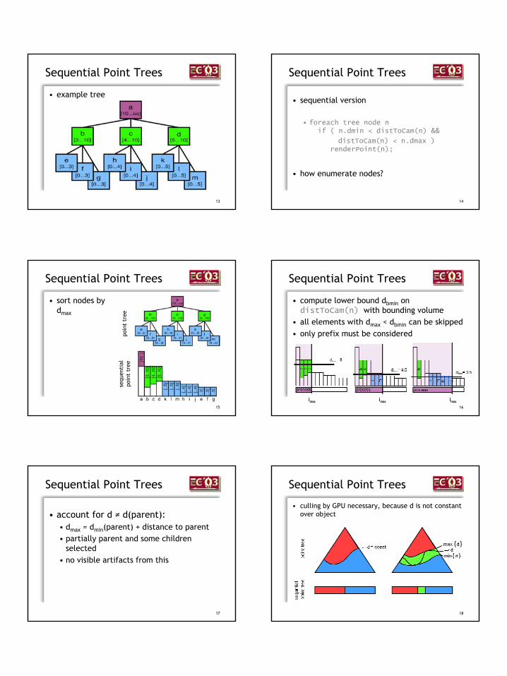
• example tree
14
Sequential Point Trees
• sequential version
• foreach tree node nif ( n.dmin < distToCam(n) &&
distToCam(n) < n.dmax )renderPoint(n);
• how enumerate nodes?
15
Sequential Point Trees
• sort nodes bydmax
poin
t tr
eese
quen
tial
poin
t tr
ee
16
imax
Sequential Point Trees
• compute lower bound dbmin on distToCam(n) with bounding volume
• all elements with dmax < dbmin can be skipped• only prefix must be considered
imax imax
17
Sequential Point Trees
• account for d ≠ d(parent):• dmax = dmin(parent) + distance to parent• partially parent and some children
selected• no visible artifacts from this
18
Sequential Point Trees
• culling by GPU necessary, because d is not constantover object
4
19
Sequential Point Trees
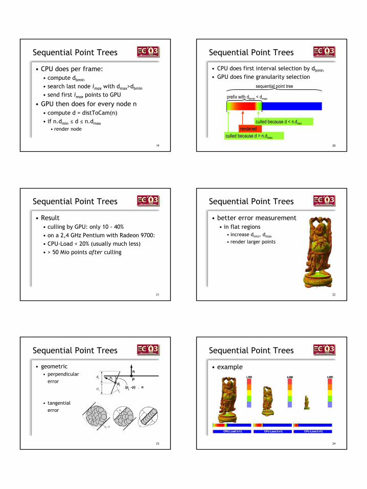
• CPU does per frame:• compute dbmin
• search last node imax with dmax>dbmin
• send first imax points to GPU
• GPU then does for every node n• compute d = distToCam(n)• if n.dmin ≤ d ≤ n.dmax
• render node
20
Sequential Point Trees
• CPU does first interval selection by dbmin
• GPU does fine granularity selection
sequential point tree
prefix with dbmin < dmax
culled because d > n.dmax
renderedculled because d < n.dmin
21
Sequential Point Trees
• Result• culling by GPU: only 10 - 40%• on a 2,4 GHz Pentium with Radeon 9700:• CPU-Load < 20% (usually much less)• > 50 Mio points after culling
22
Sequential Point Trees
• better error measurement• in flat regions
• increase dmin, dmax
• render larger points
23
Sequential Point Trees
• geometric• perpendicular
error
• tangentialerror
24
Sequential Point Trees
• example
5
25
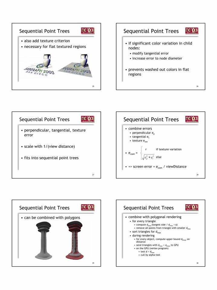
Sequential Point Trees
• also add texture criterion• necessary for flat textured regions
26
Sequential Point Trees
• if significant color variation in childnodes:• modify tangential error• increase error to node diameter
• prevents washed out colors in flatregions
27
Sequential Point Trees
• perpendicular, tangential, textureerror
• scale with 1/(view distance)
• fits into sequential point trees
28
Sequential Point Trees
• combine errors• perpendicular ep
• tangential et
• texture etex
• ecom =
• => screen error = ecom / viewDistance
r if texture variation
else22tp ee +
29
Sequential Point Trees
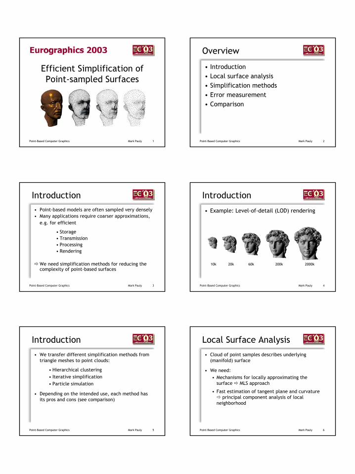
• can be combined with polygons
30
Sequential Point Trees
• combine with polygonal rendering• for every triangle
• compute dmax (longest side / dmax = ε)• remove all points from triangle with smaller dmax
• sort triangles for dmax
• during rendering• for every object, compute upper bound dbmax on
distance• send triangles with dmax < dbmax to GPU• on the GPU (vertex program)
• test d < dmax
• cull by alpha-test

6
31
Sequential Point Trees
• pros• very simple!• CPU-load low• most work moved to GPU• GPU runs at maximum efficiency
• cons• no view frustum culling• currently: bad splatting support by GPU
1
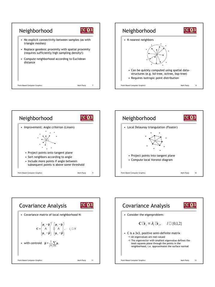
Point-Based Computer Graphics Mark Pauly 1
Efficient Simplification of Point-sampled Surfaces
Point-Based Computer Graphics Mark Pauly 2
Overview
• Introduction• Local surface analysis• Simplification methods• Error measurement• Comparison
Point-Based Computer Graphics Mark Pauly 3
Introduction• Point-based models are often sampled very densely• Many applications require coarser approximations,
e.g. for efficient
• Storage• Transmission• Processing• Rendering
We need simplification methods for reducing the complexity of point-based surfaces
Point-Based Computer Graphics Mark Pauly 4
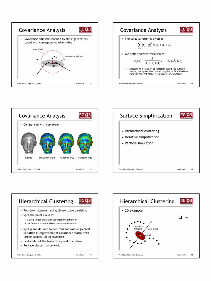
Introduction
• Example: Level-of-detail (LOD) rendering
10k 20k 60k 200k 2000k
Point-Based Computer Graphics Mark Pauly 5
Introduction
• We transfer different simplification methods from triangle meshes to point clouds:
• Hierarchical clustering• Iterative simplification• Particle simulation
• Depending on the intended use, each method has its pros and cons (see comparison)
Point-Based Computer Graphics Mark Pauly 6
Local Surface Analysis
• Cloud of point samples describes underlying (manifold) surface
• We need:• Mechanisms for locally approximating the
surface MLS approach
• Fast estimation of tangent plane and curvature principal component analysis of local
neighborhood
2
Point-Based Computer Graphics Mark Pauly 7
Neighborhood
• No explicit connectivity between samples (as with triangle meshes)
• Replace geodesic proximity with spatial proximity (requires sufficiently high sampling density!)
• Compute neighborhood according to Euclidean distance
Point-Based Computer Graphics Mark Pauly 8
Neighborhood
• K-nearest neighbors
• Can be quickly computed using spatial data-structures (e.g. kd-tree, octree, bsp-tree)
• Requires isotropic point distribution
Point-Based Computer Graphics Mark Pauly 9
Neighborhood
• Improvement: Angle criterion (Linsen)
• Project points onto tangent plane• Sort neighbors according to angle• Include more points if angle between
subsequent points is above some threshold
Point-Based Computer Graphics Mark Pauly 10
Neighborhood
• Local Delaunay triangulation (Floater)
• Project points into tangent plane• Compute local Voronoi diagram
Point-Based Computer Graphics Mark Pauly 11
Covariance Analysis
• Covariance matrix of local neighborhood N:
• with centroid
Ni ji
i
T
i
i
nn
∈
−
−⋅
−
−= ,
11
pp
pp
pp
ppC ΛΛ
∑∈
=Ni
iNpp 1
Point-Based Computer Graphics Mark Pauly 12
Covariance Analysis
• Consider the eigenproblem:
• C is a 3x3, positive semi-definite matrixAll eigenvalues are real-valuedThe eigenvector with smallest eigenvalue defines the least-squares plane through the points in the neighborhood, i.e. approximates the surface normal
2,1,0, ∈⋅=⋅ llll vvC λ
3
Point-Based Computer Graphics Mark Pauly 13
Covariance Analysis
• Covariance ellipsoid spanned by the eigenvectors scaled with corresponding eigenvalue
Point-Based Computer Graphics Mark Pauly 14
Covariance Analysis• The total variation is given as:
• We define surface variation as:
• Measures the fraction of variation along the surface normal, i.e. quantifies how strong the surface deviates from the tangent plane estimate for curvature
210210
0 ,)( λλλλλλ
λσ ≤≤++
=pn
2102 λλλ ++=−∑
∈ Nii pp
Point-Based Computer Graphics Mark Pauly 15
Covariance Analysis
• Comparison with curvature:
original mean curvature variation n=20 variation n=50
Point-Based Computer Graphics Mark Pauly 16
Surface Simplification
• Hierarchical clustering
• Iterative simplification
• Particle simulation
Point-Based Computer Graphics Mark Pauly 17
Hierarchical Clustering
• Top-down approach using binary space partition:
• Split the point cloud if:
• Size is larger than user-specified maximum or
• Surface variation is above maximum threshold
• Split plane defined by centroid and axis of greatest variation (= eigenvector of covariance matrix with largest associated eigenvector)
• Leaf nodes of the tree correspond to clusters• Replace clusters by centroid
Point-Based Computer Graphics Mark Pauly 18
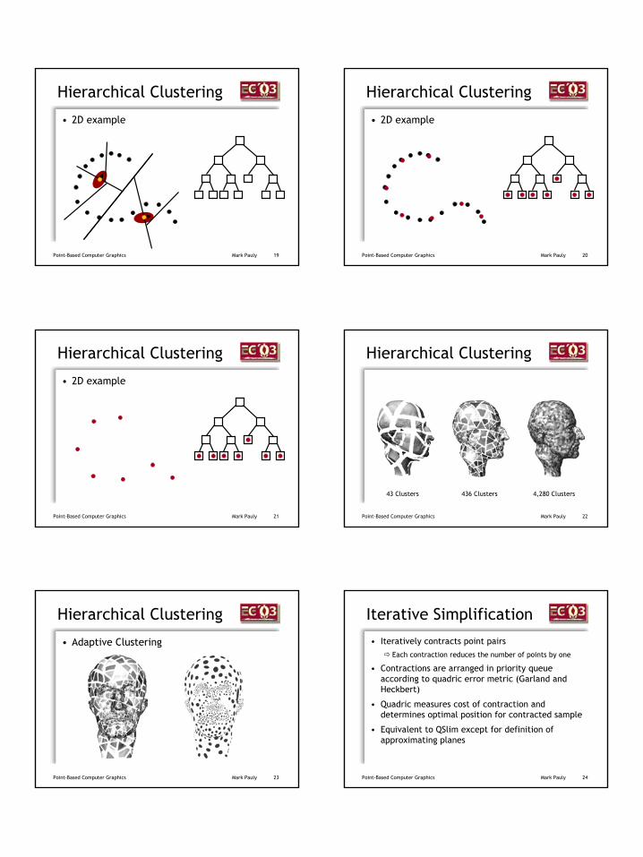
Hierarchical Clustering
• 2D example
covariance ellipsoid split plane
centroid
root
4
Point-Based Computer Graphics Mark Pauly 19
Hierarchical Clustering
• 2D example
Point-Based Computer Graphics Mark Pauly 20
Hierarchical Clustering
• 2D example
Point-Based Computer Graphics Mark Pauly 21
Hierarchical Clustering
• 2D example
Point-Based Computer Graphics Mark Pauly 22
Hierarchical Clustering
4,280 Clusters436 Clusters43 Clusters
Point-Based Computer Graphics Mark Pauly 23
Hierarchical Clustering
• Adaptive Clustering
Point-Based Computer Graphics Mark Pauly 24
Iterative Simplification
• Iteratively contracts point pairsEach contraction reduces the number of points by one
• Contractions are arranged in priority queue according to quadric error metric (Garland and Heckbert)
• Quadric measures cost of contraction and determines optimal position for contracted sample
• Equivalent to QSlim except for definition of approximating planes
5
Point-Based Computer Graphics Mark Pauly 25
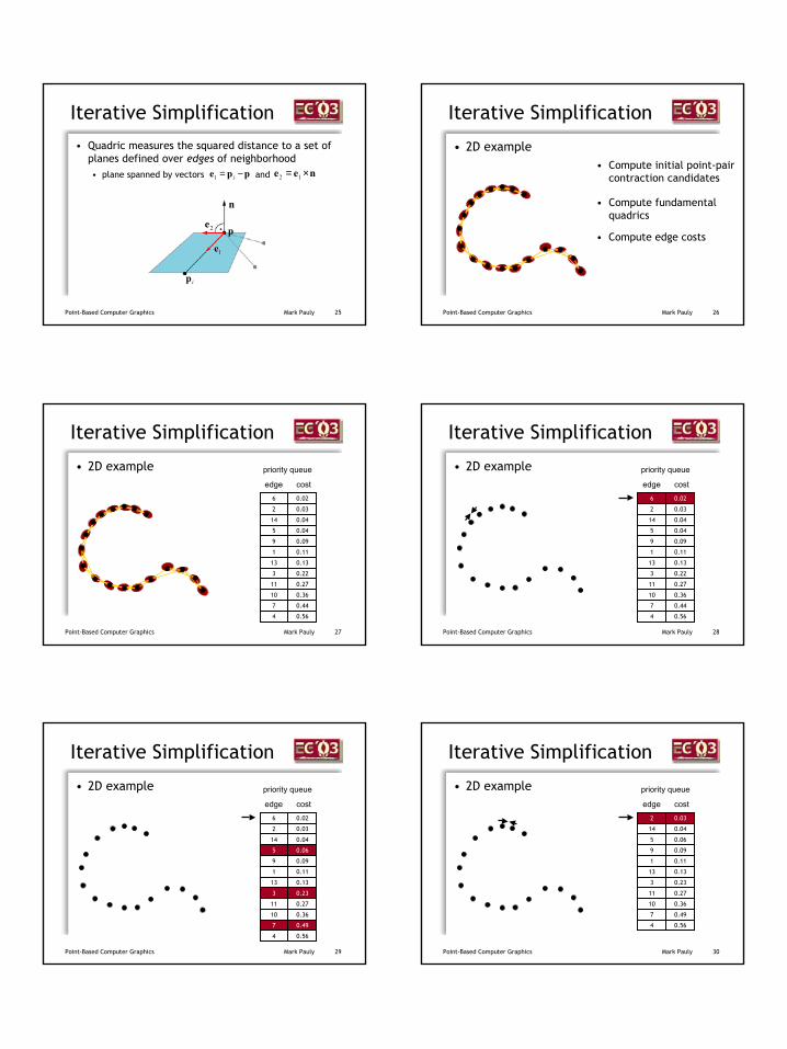
Iterative Simplification
• Quadric measures the squared distance to a set of planes defined over edges of neighborhood• plane spanned by vectors andppe −= i1 nee ×= 12
1e
ip
p2e
n
Point-Based Computer Graphics Mark Pauly 26
Iterative Simplification
• 2D example
• Compute fundamental quadrics
• Compute initial point-pair contraction candidates
• Compute edge costs
Point-Based Computer Graphics Mark Pauly 27
Iterative Simplification
• 2D example
0.564
0.447
0.3610
0.2711
0.223
0.1313
0.111
0.099
0.045
0.0414
0.032
0.026
priority queue
edge cost
Point-Based Computer Graphics Mark Pauly 28
Iterative Simplification
• 2D example
0.564
0.447
0.3610
0.2711
0.223
0.1313
0.111
0.099
0.045
0.0414
0.032
0.026
priority queue
edge cost
Point-Based Computer Graphics Mark Pauly 29
Iterative Simplification
• 2D example
0.564
0.497
0.3610
0.2711
0.233
0.1313
0.111
0.099
0.065
0.0414
0.032
0.026
priority queue
edge cost
Point-Based Computer Graphics Mark Pauly 30
Iterative Simplification
• 2D example
0.564
0.497
0.3610
0.2711
0.233
0.1313
0.111
0.099
0.065
0.0414
0.032
priority queue
edge cost
6
Point-Based Computer Graphics Mark Pauly 31
Iterative Simplification
• 2D example
0.564
0.497
0.3610
0.2711
0.233
0.1313
0.111
0.099
0.065
0.0414
0.032
priority queue
edge cost
Point-Based Computer Graphics Mark Pauly 32
Iterative Simplification
• 2D example
0.564
0.497
0.3610
0.2711
0.233
0.1313
0.111
0.099
0.065
0.0414
priority queue
edge cost
Point-Based Computer Graphics Mark Pauly 33
Iterative Simplification
• 2D example
0.564
0.497
0.3610
0.2711
priority queue
edge cost
Point-Based Computer Graphics Mark Pauly 34
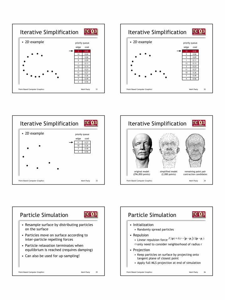
Iterative Simplification
original model (296,850 points)
simplified model (2,000 points)
remaining point pair contraction candidates
Point-Based Computer Graphics Mark Pauly 35
Particle Simulation
• Resample surface by distributing particles on the surface
• Particles move on surface according to inter-particle repelling forces
• Particle relaxation terminates when equilibrium is reached (requires damping)
• Can also be used for up-sampling!
Point-Based Computer Graphics Mark Pauly 36
Particle Simulation
• Initialization• Randomly spread particles
• Repulsion• Linear repulsion force
only need to consider neighborhood of radius r
• Projection• Keep particles on surface by projecting onto
tangent plane of closest point• Apply full MLS projection at end of simulation
)()()( iii rkF ppppp −⋅−−=
7
Point-Based Computer Graphics Mark Pauly 37
Particle Simulation
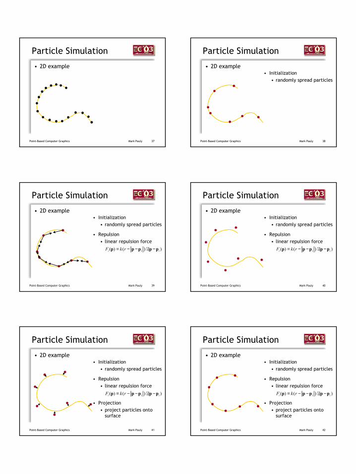
• 2D example
Point-Based Computer Graphics Mark Pauly 38
Particle Simulation
• 2D example• Initialization
• randomly spread particles
Point-Based Computer Graphics Mark Pauly 39
Particle Simulation
• 2D example
• Repulsion• linear repulsion force
)()()( iii rkF ppppp −⋅−−=
• Initialization• randomly spread particles
Point-Based Computer Graphics Mark Pauly 40
Particle Simulation
• 2D example
• Repulsion• linear repulsion force
)()()( iii rkF ppppp −⋅−−=
• Initialization• randomly spread particles
Point-Based Computer Graphics Mark Pauly 41
Particle Simulation
• 2D example
• Repulsion• linear repulsion force
)()()( iii rkF ppppp −⋅−−=
• Initialization• randomly spread particles
• Projection• project particles onto
surface
Point-Based Computer Graphics Mark Pauly 42
Particle Simulation
• 2D example
• Repulsion• linear repulsion force
)()()( iii rkF ppppp −⋅−−=
• Initialization• randomly spread particles
• Projection• project particles onto
surface
8
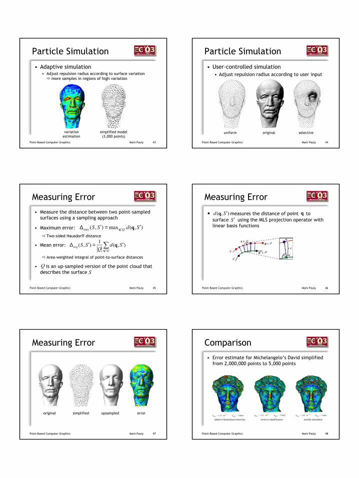
Point-Based Computer Graphics Mark Pauly 43
Particle Simulation
• Adaptive simulation• Adjust repulsion radius according to surface variation
more samples in regions of high variation
variation estimation
simplified model (3,000 points)
Point-Based Computer Graphics Mark Pauly 44
Particle Simulation
• User-controlled simulation• Adjust repulsion radius according to user input
uniform original selective
Point-Based Computer Graphics Mark Pauly 45
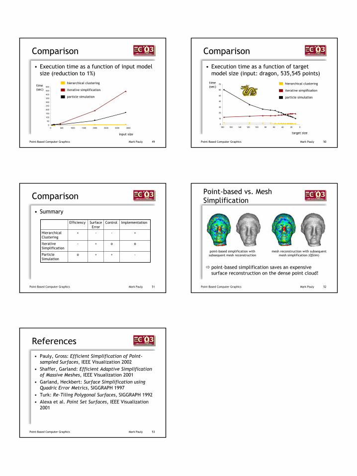
Measuring Error
• Measure the distance between two point-sampled surfaces using a sampling approach
• Maximum error:
Two-sided Hausdorff distance
• Mean error:
Area-weighted integral of point-to-surface distances
• is an up-sampled version of the point cloud that describes the surface
),(max),(max SdSS Q ′=′∆ ∈ qq
∑∈
′=′∆Q
SdQ
SSq
q ),(1),(avg
SQ
Point-Based Computer Graphics Mark Pauly 46
Measuring Error
• measures the distance of point to surface using the MLS projection operator with linear basis functions
),( Sd ′q qS ′
Point-Based Computer Graphics Mark Pauly 47
Measuring Error
original simplified upsampled error
Point-Based Computer Graphics Mark Pauly 48
Comparison
• Error estimate for Michelangelo’s David simplified from 2,000,000 points to 5,000 points
9
Point-Based Computer Graphics Mark Pauly 49
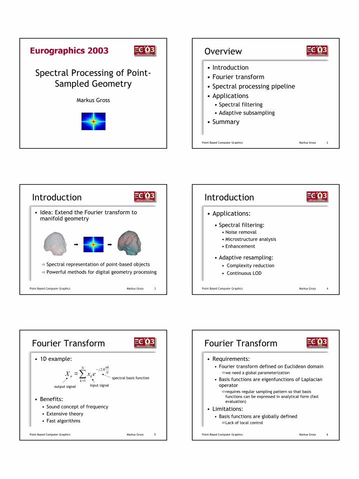
Comparison
• Execution time as a function of input model size (reduction to 1%)
0
50
100
150
200
250
300
350
400
450
500
0 500 1000 1500 2000 2500 3000 3500
hierarchical clustering
iterative simplification
particle simulation
time (sec)
input size
Point-Based Computer Graphics Mark Pauly 50
Comparison
• Execution time as a function of target model size (input: dragon, 535,545 points)
0
10
20
30
40
50
60
70
020406080100120140160180
hierarchical clustering
iterative simplification
particle simulation
target size
time (sec)
Point-Based Computer Graphics Mark Pauly 51
Comparison
• Summary
-
o
+
Implementation
++oParticle Simulation
o+-Iterative Simplification
--+Hierarchical Clustering
ControlSurface Error
Efficiency
Point-Based Computer Graphics Mark Pauly 52
Point-based vs. Mesh Simplification
point-based simplification saves an expensive surface reconstruction on the dense point cloud!
point-based simplification with subsequent mesh reconstruction
mesh reconstruction with subsequent mesh simplification (QSlim)
Point-Based Computer Graphics Mark Pauly 53
References
• Pauly, Gross: Efficient Simplification of Point-sampled Surfaces, IEEE Visualization 2002
• Shaffer, Garland: Efficient Adaptive Simplification of Massive Meshes, IEEE Visualization 2001
• Garland, Heckbert: Surface Simplification using Quadric Error Metrics, SIGGRAPH 1997
• Turk: Re-Tiling Polygonal Surfaces, SIGGRAPH 1992• Alexa et al. Point Set Surfaces, IEEE Visualization
2001
1
Spectral Processing of Point-Sampled Geometry
Markus Gross
2Point-Based Computer Graphics Markus Gross
Overview
• Introduction• Fourier transform• Spectral processing pipeline• Applications
• Spectral filtering• Adaptive subsampling
• Summary
3Point-Based Computer Graphics Markus Gross
Introduction
• Idea: Extend the Fourier transform to manifold geometry
Spectral representation of point-based objects
Powerful methods for digital geometry processing
4Point-Based Computer Graphics Markus Gross
Introduction
• Applications:
• Spectral filtering:• Noise removal • Microstructure analysis• Enhancement
• Adaptive resampling:• Complexity reduction
• Continuous LOD
5Point-Based Computer Graphics Markus Gross
Fourier Transform
• 1D example:
• Benefits:• Sound concept of frequency• Extensive theory• Fast algorithms
∑=
−=
N
k
Nnkj
kn exX1
2π
input signal
spectral basis function
output signal
6Point-Based Computer Graphics Markus Gross
Fourier Transform
• Requirements:• Fourier transform defined on Euclidean domain
we need a global parameterization
• Basis functions are eigenfunctions of Laplacian operator
requires regular sampling pattern so that basis functions can be expressed in analytical form (fast evaluation)
• Limitations:• Basis functions are globally defined
Lack of local control
2
7Point-Based Computer Graphics Markus Gross
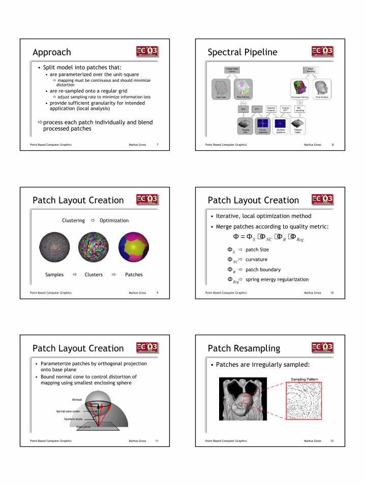
Approach
• Split model into patches that:• are parameterized over the unit-square
mapping must be continuous and should minimize distortion
• are re-sampled onto a regular gridadjust sampling rate to minimize information loss
• provide sufficient granularity for intended application (local analysis)
process each patch individually and blend processed patches
8Point-Based Computer Graphics Markus Gross
Spectral Pipeline
9Point-Based Computer Graphics Markus Gross
Patch Layout Creation
Clustering Optimization
Samples Clusters Patches
10Point-Based Computer Graphics Markus Gross
Patch Layout Creation
• Iterative, local optimization method
• Merge patches according to quality metric:
RegBNCS Φ⋅Φ⋅Φ⋅Φ=Φ
curvature
patch Size
patch boundary
spring energy regularization
NCΦ
BΦ
RegΦ
SΦ
11Point-Based Computer Graphics Markus Gross
Patch Layout Creation
• Parameterize patches by orthogonal projection onto base plane
• Bound normal cone to control distortion of mapping using smallest enclosing sphere
12Point-Based Computer Graphics Markus Gross
Patch Resampling
• Patches are irregularly sampled:
3
13Point-Based Computer Graphics Markus Gross
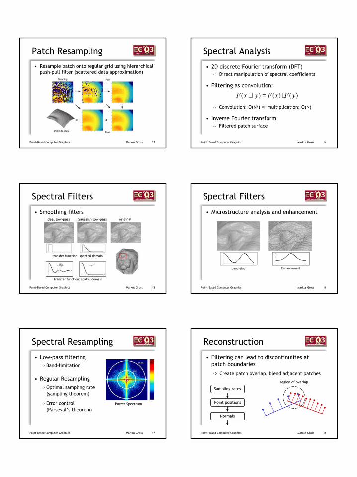
Patch Resampling
• Resample patch onto regular grid using hierarchical push-pull filter (scattered data approximation)
14Point-Based Computer Graphics Markus Gross
Spectral Analysis
• 2D discrete Fourier transform (DFT)Direct manipulation of spectral coefficients
• Filtering as convolution:
Convolution: O(N2) multiplication: O(N)
• Inverse Fourier transformFiltered patch surface
)()()( yFxFyxF ⋅=⊗
15Point-Based Computer Graphics Markus Gross
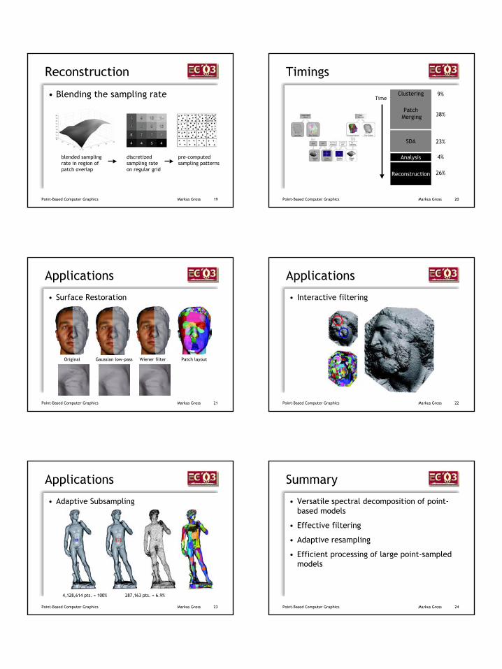
Spectral Filters
ideal low-pass Gaussian low-pass original
transfer function: spectral domain
transfer function: spatial domain
• Smoothing filters
16Point-Based Computer Graphics Markus Gross
Spectral Filters
• Microstructure analysis and enhancement
17Point-Based Computer Graphics Markus Gross
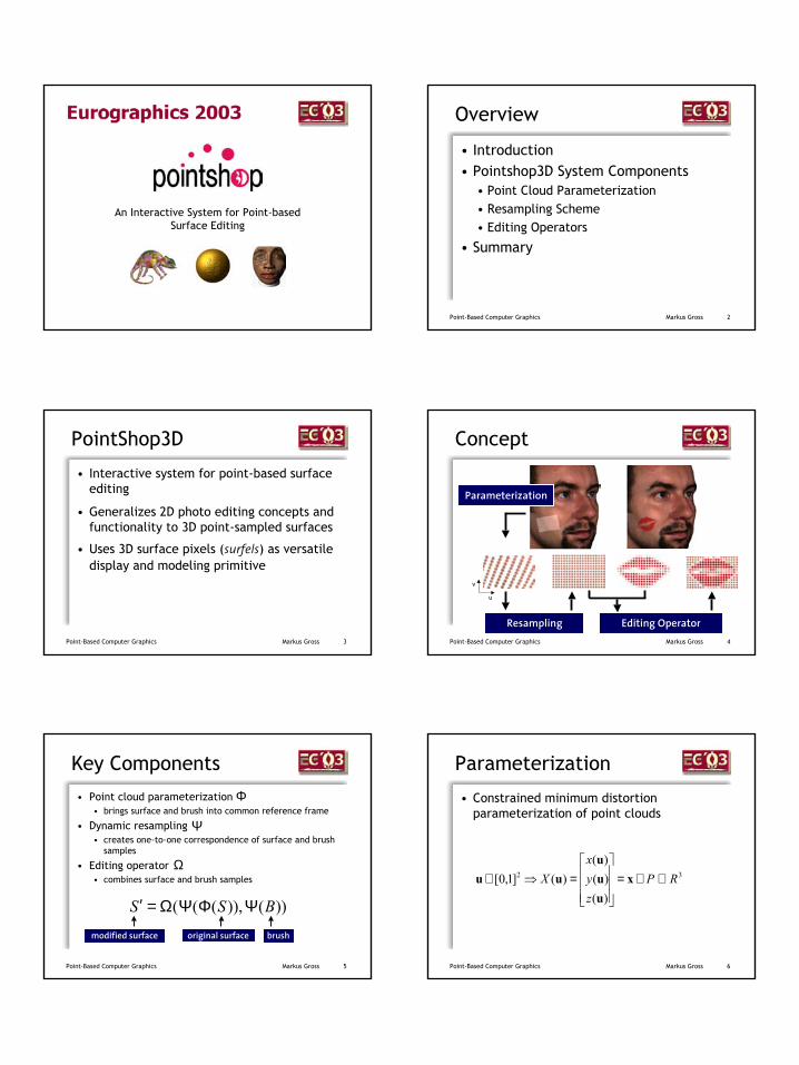
Spectral Resampling
• Low-pass filteringBand-limitation
• Regular ResamplingOptimal sampling rate (sampling theorem)
Error control (Parseval’s theorem)
Power Spectrum
18Point-Based Computer Graphics Markus Gross
Reconstruction
• Filtering can lead to discontinuities at patch boundaries
Create patch overlap, blend adjacent patches
region of overlap
Sampling rates
Point positions
Normals
4
19Point-Based Computer Graphics Markus Gross
Reconstruction
• Blending the sampling rate
blended sampling rate in region of patch overlap
discretizedsampling rate on regular grid
pre-computed sampling patterns
20Point-Based Computer Graphics Markus Gross
Timings
Clustering
PatchMerging
SDA
Analysis
Reconstruction
Time9%
38%
23%
4%
26%
21Point-Based Computer Graphics Markus Gross
Applications
• Surface Restoration
Original Gaussian low-pass Wiener filter Patch layout
22Point-Based Computer Graphics Markus Gross
Applications
• Interactive filtering
23Point-Based Computer Graphics Markus Gross
Applications
• Adaptive Subsampling
4,128,614 pts. = 100% 287,163 pts. = 6.9%
24Point-Based Computer Graphics Markus Gross
Summary
• Versatile spectral decomposition of point-based models
• Effective filtering
• Adaptive resampling
• Efficient processing of large point-sampled models

5
25Point-Based Computer Graphics Markus Gross
Reference
• Pauly, Gross: Spectral Processing of Point-sampled Geometry, SIGGRAPH 2001
1
An Interactive System for Point-based Surface Editing
2Point-Based Computer Graphics Markus Gross
Overview
• Introduction• Pointshop3D System Components
• Point Cloud Parameterization• Resampling Scheme• Editing Operators
• Summary
3Point-Based Computer Graphics Markus Gross
PointShop3D
• Interactive system for point-based surface editing
• Generalizes 2D photo editing concepts and functionality to 3D point-sampled surfaces
• Uses 3D surface pixels (surfels) as versatile display and modeling primitive
4Point-Based Computer Graphics Markus Gross
Concept
Resampling Editing Operator
u
Parameterization
v
5Point-Based Computer Graphics Markus Gross
• Point cloud parameterization• brings surface and brush into common reference frame
• Dynamic resampling• creates one-to-one correspondence of surface and brush
samples
• Editing operator• combines surface and brush samples
Key Components
Φ
))()),((( BSS ΨΦΨΩ=′
Ψ
Ω
brushoriginal surfacemodified surface
6Point-Based Computer Graphics Markus Gross
Parameterization
• Constrained minimum distortion parameterization of point clouds
32
)()()(
)(]1,0[ RPzyx
X ⊂∈=
=⇒∈ x
uuu
uu
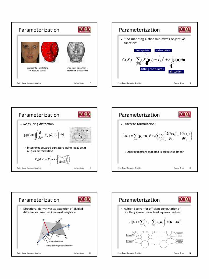
2
7Point-Based Computer Graphics Markus Gross
Parameterization
contraints = matching of feature points
minimum distortion = maximum smoothness
8Point-Based Computer Graphics Markus Gross
Parameterization
• Find mapping X that minimizes objective function:
∑ ∫∈
+−=Mj P
jj dXXC uuxp )())(()( 2 γε
fitting constraintsdistortion
surface pointsbrush points
9Point-Based Computer Graphics Markus Gross
Parameterization
• Measuring distortion
• Integrates squared curvature using local polar re-parameterization
θθγθ
drXr
2
2
2
),()( ∫
∂∂= uu
θ
ur
+=
)sin()cos(
),(θθ
θ rXrX uu
10Point-Based Computer Graphics Markus Gross
Parameterization
• Discrete formulation:
• Approximation: mapping is piecewise linear
2
1
2~)()()()(~ ∑ ∑∑
∈ = ∈
∂∂−
∂∂+−=
Mj
n
i Nj j
i
j
ijj
i
UUUCvx
vxp εu
11Point-Based Computer Graphics Markus Gross
Parameterization
• Directional derivatives as extension of divided differences based on k-nearest neighbors
12Point-Based Computer Graphics Markus Gross
Parameterization
• Multigrid solver for efficient computation of resulting sparse linear least squares problem
22
1,)(~ ubub AaUC
ji
n
iijj −=
−=∑ ∑=
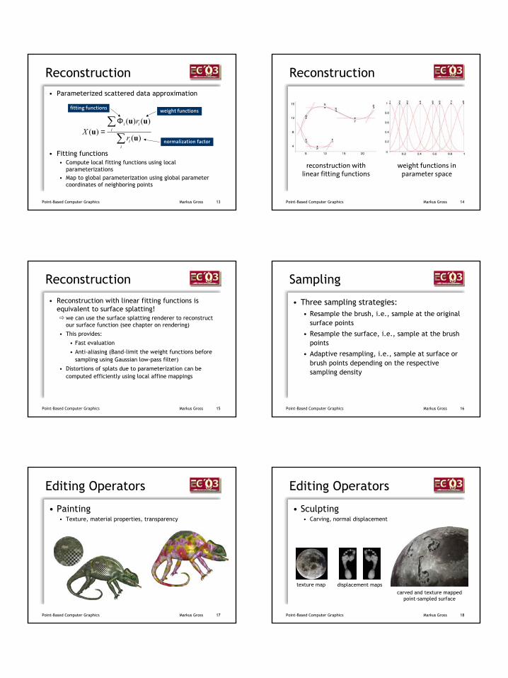
3
13Point-Based Computer Graphics Markus Gross
Reconstruction• Parameterized scattered data approximation
• Fitting functions• Compute local fitting functions using local
parameterizations• Map to global parameterization using global parameter
coordinates of neighboring points
∑∑Φ
=
ii
iii
r
rX
)(
)()()(
u
uuu
fitting functions weight functions
normalization factor
14Point-Based Computer Graphics Markus Gross
Reconstruction
reconstruction with linear fitting functions
weight functions in parameter space
15Point-Based Computer Graphics Markus Gross
Reconstruction
• Reconstruction with linear fitting functions is equivalent to surface splatting!
we can use the surface splatting renderer to reconstruct our surface function (see chapter on rendering)
• This provides:
• Fast evaluation
• Anti-aliasing (Band-limit the weight functions before sampling using Gaussian low-pass filter)
• Distortions of splats due to parameterization can be computed efficiently using local affine mappings
16Point-Based Computer Graphics Markus Gross
Sampling
• Three sampling strategies:• Resample the brush, i.e., sample at the original
surface points
• Resample the surface, i.e., sample at the brush points
• Adaptive resampling, i.e., sample at surface or brush points depending on the respective sampling density
17Point-Based Computer Graphics Markus Gross
Editing Operators
• Painting• Texture, material properties, transparency
18Point-Based Computer Graphics Markus Gross
Editing Operators
• Sculpting• Carving, normal displacement
displacement mapstexture mapcarved and texture mapped
point-sampled surface
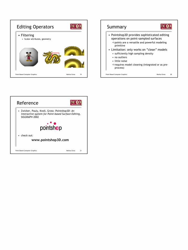
4
19Point-Based Computer Graphics Markus Gross
Editing Operators
• Filtering• Scalar attributes, geometry
20Point-Based Computer Graphics Markus Gross
Summary
• Pointshop3D provides sophisticated editing operations on point-sampled surfaces
points are a versatile and powerful modeling primitive
• Limitation: only works on “clean” models• sufficiently high sampling density• no outliers• little noise
requires model cleaning (integrated or as pre-process)
21Point-Based Computer Graphics Markus Gross
Reference
• Zwicker, Pauly, Knoll, Gross: Pointshop3D: An interactive system for Point-based Surface Editing, SIGGRAPH 2002
• check out:
www.pointshop3D.com
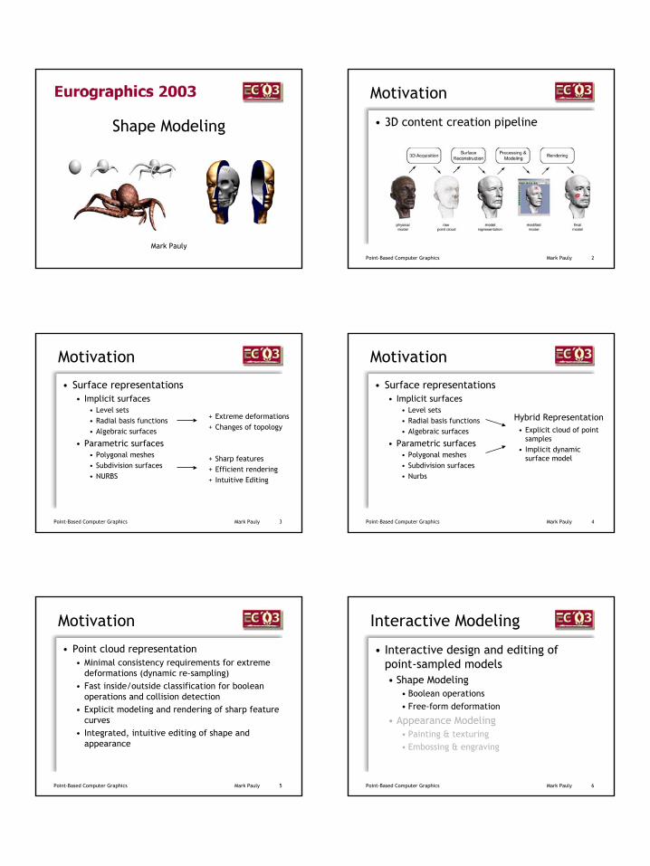
1
Shape Modeling
Mark Pauly
2Point-Based Computer Graphics Mark Pauly
Motivation
• 3D content creation pipeline
3Point-Based Computer Graphics Mark Pauly
Motivation
• Surface representations• Implicit surfaces
• Level sets• Radial basis functions• Algebraic surfaces
• Parametric surfaces• Polygonal meshes• Subdivision surfaces• NURBS
+ Extreme deformations+ Changes of topology
+ Sharp features+ Efficient rendering+ Intuitive Editing
4Point-Based Computer Graphics Mark Pauly
Motivation
• Surface representations• Implicit surfaces
• Level sets• Radial basis functions• Algebraic surfaces
• Parametric surfaces• Polygonal meshes• Subdivision surfaces• Nurbs
Hybrid Representation• Explicit cloud of point
samples• Implicit dynamic
surface model
5Point-Based Computer Graphics Mark Pauly
Motivation
• Point cloud representation• Minimal consistency requirements for extreme
deformations (dynamic re-sampling)• Fast inside/outside classification for boolean
operations and collision detection• Explicit modeling and rendering of sharp feature
curves• Integrated, intuitive editing of shape and
appearance
6Point-Based Computer Graphics Mark Pauly
Interactive Modeling
• Interactive design and editing of point-sampled models• Shape Modeling
• Boolean operations• Free-form deformation
• Appearance Modeling• Painting & texturing• Embossing & engraving
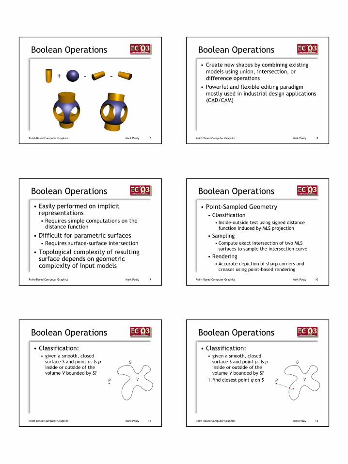
2
7Point-Based Computer Graphics Mark Pauly
Boolean Operations
+ - -
8Point-Based Computer Graphics Mark Pauly
Boolean Operations
• Create new shapes by combining existing models using union, intersection, or difference operations
• Powerful and flexible editing paradigm mostly used in industrial design applications (CAD/CAM)
9Point-Based Computer Graphics Mark Pauly
Boolean Operations
• Easily performed on implicit representations• Requires simple computations on the
distance function
• Difficult for parametric surfaces• Requires surface-surface intersection
• Topological complexity of resulting surface depends on geometric complexity of input models
10Point-Based Computer Graphics Mark Pauly
Boolean Operations
• Point-Sampled Geometry• Classification
• Inside-outside test using signed distance function induced by MLS projection
• Sampling• Compute exact intersection of two MLS
surfaces to sample the intersection curve
• Rendering• Accurate depiction of sharp corners and
creases using point-based rendering
11Point-Based Computer Graphics Mark Pauly
Boolean Operations
• Classification:• given a smooth, closed
surface S and point p. Is p inside or outside of the volume V bounded by S?
S
p V
12Point-Based Computer Graphics Mark Pauly
Boolean Operations
• Classification:• given a smooth, closed
surface S and point p. Is p inside or outside of the volume V bounded by S?
1.find closest point q on S
S
p
q
V
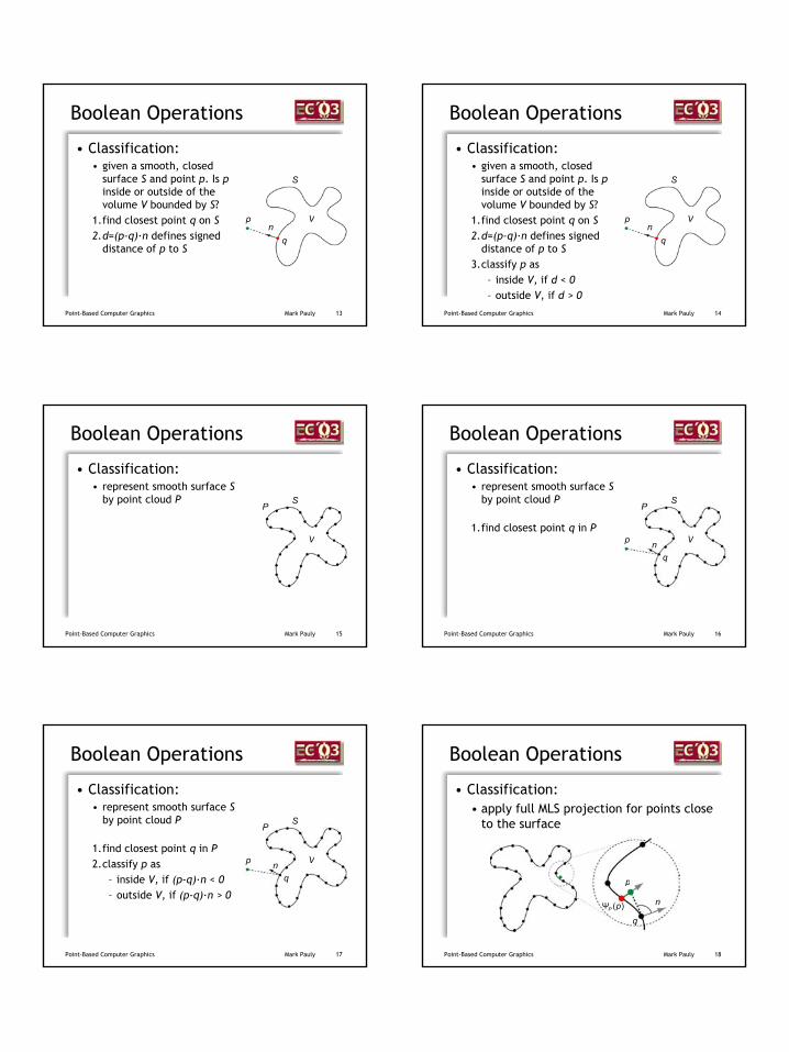
3
13Point-Based Computer Graphics Mark Pauly
Boolean Operations
• Classification:• given a smooth, closed
surface S and point p. Is p inside or outside of the volume V bounded by S?
1.find closest point q on S2.d=(p-q)·n defines signed
distance of p to S
p
qn
S
V
14Point-Based Computer Graphics Mark Pauly
Boolean Operations
• Classification:• given a smooth, closed
surface S and point p. Is p inside or outside of the volume V bounded by S?
1.find closest point q on S2.d=(p-q)·n defines signed
distance of p to S 3.classify p as
– inside V, if d < 0– outside V, if d > 0
p
qn
S
V
15Point-Based Computer Graphics Mark Pauly
Boolean Operations
• Classification:• represent smooth surface S
by point cloud Pm P
S
V
16Point-Based Computer Graphics Mark Pauly
Boolean Operations
• Classification:• represent smooth surface S
by point cloud Pm
1.find closest point q in Pp
P
qn
S
V
17Point-Based Computer Graphics Mark Pauly
Boolean Operations
• Classification:• represent smooth surface S
by point cloud Pm
1.find closest point q in P2.classify p as
– inside V, if (p-q)·n < 0– outside V, if (p-q)·n > 0
p
P
qn
S
V
18Point-Based Computer Graphics Mark Pauly
Boolean Operations
• Classification:• apply full MLS projection for points close
to the surface
q
p
n)(pPΨ
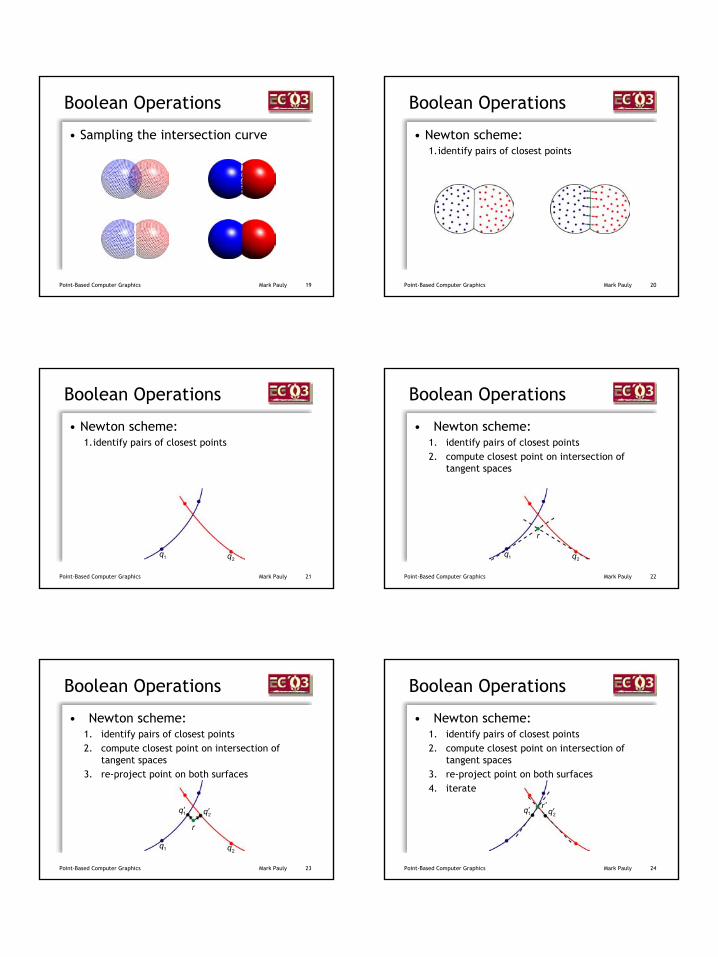
4
19Point-Based Computer Graphics Mark Pauly
Boolean Operations
• Sampling the intersection curve
20Point-Based Computer Graphics Mark Pauly
Boolean Operations
• Newton scheme:1.identify pairs of closest points
21Point-Based Computer Graphics Mark Pauly
Boolean Operations
• Newton scheme:1.identify pairs of closest points
1q 2q
22Point-Based Computer Graphics Mark Pauly
Boolean Operations
• Newton scheme:1. identify pairs of closest points2. compute closest point on intersection of
tangent spaces
r
1q 2q
23Point-Based Computer Graphics Mark Pauly
Boolean Operations
• Newton scheme:1. identify pairs of closest points2. compute closest point on intersection of
tangent spaces3. re-project point on both surfaces
1q′2q′
r
1q 2q
24Point-Based Computer Graphics Mark Pauly
Boolean Operations
• Newton scheme:1. identify pairs of closest points2. compute closest point on intersection of
tangent spaces3. re-project point on both surfaces4. iterate
r ′1q′
2q′
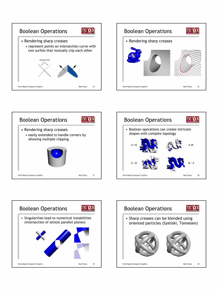
5
25Point-Based Computer Graphics Mark Pauly
Boolean Operations
• Rendering sharp creases• represent points on intersection curve with
two surfels that mutually clip each other
26Point-Based Computer Graphics Mark Pauly
Boolean Operations
• Rendering sharp creases
27Point-Based Computer Graphics Mark Pauly
Boolean Operations
• Rendering sharp creases• easily extended to handle corners by
allowing multiple clipping
28Point-Based Computer Graphics Mark Pauly
Boolean Operations
• Boolean operations can create intricate shapes with complex topology
BA + BA ⋅
BA − AB −
29Point-Based Computer Graphics Mark Pauly
Boolean Operations
• Singularities lead to numerical instabilities (intersection of almost parallel planes)
30Point-Based Computer Graphics Mark Pauly
Boolean Operations
• Sharp creases can be blended using oriented particles (Szeliski, Tonnesen)
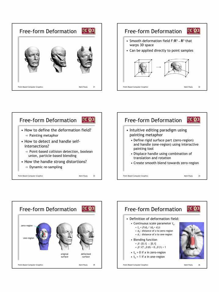
6
31Point-Based Computer Graphics Mark Pauly
Free-form Deformation
32Point-Based Computer Graphics Mark Pauly
Free-form Deformation
• Smooth deformation field F:R3→R3 that warps 3D space
• Can be applied directly to point samples
33Point-Based Computer Graphics Mark Pauly
Free-form Deformation
• How to define the deformation field?Painting metaphor
• How to detect and handle self-intersections?
Point-based collision detection, boolean union, particle-based blending
• How the handle strong distortions?Dynamic re-sampling
34Point-Based Computer Graphics Mark Pauly
Free-form Deformation
• Intuitive editing paradigm using painting metaphor• Define rigid surface part (zero-region)
and handle (one-region) using interactive painting tool
• Displace handle using combination of translation and rotation
• Create smooth blend towards zero-region
35Point-Based Computer Graphics Mark Pauly
Free-form Deformation
one-region
zero-region
originalsurface
deformedsurface
36Point-Based Computer Graphics Mark Pauly
Free-form Deformation
• Definition of deformation field:• Continuous scale parameter tx
• tx = β (d0 / (d0 + d1))• d0 : distance of x to zero-region• d1 : distance of x to one-region
• Blending function • β : [0,1] → [0,1]• β ∈ C0, β (0) = 0, β (1) = 1
• tx = 0 if x in zero-region• tx = 1 if x in one-region
xd0
d1
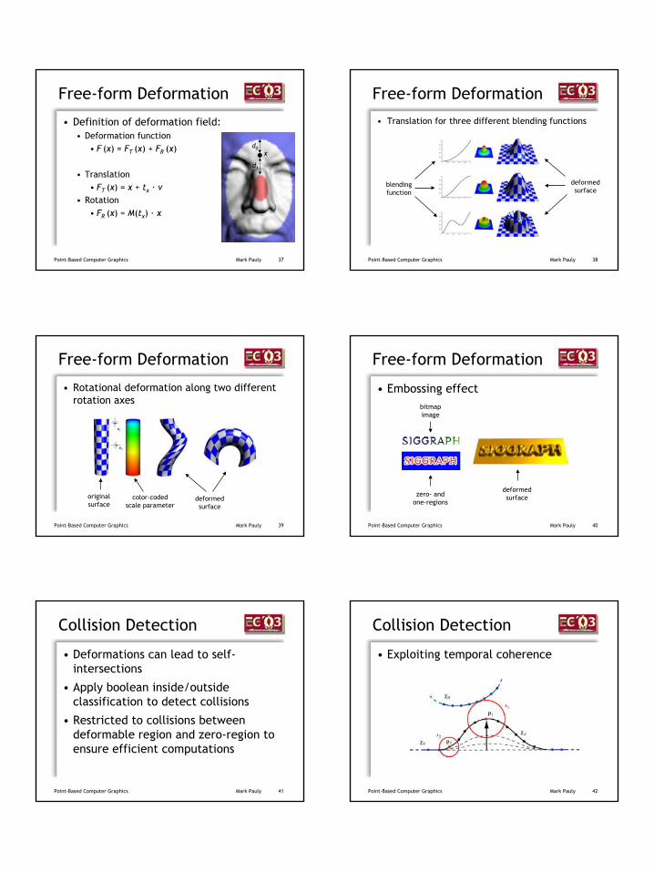
7
37Point-Based Computer Graphics Mark Pauly
Free-form Deformation
• Definition of deformation field:• Deformation function
• F (x) = FT (x) + FR (x)
• Translation• FT (x) = x + tx · v
• Rotation• FR (x) = M(tx) · x
xd0
d1
38Point-Based Computer Graphics Mark Pauly
Free-form Deformation
• Translation for three different blending functions
blendingfunction
deformedsurface
39Point-Based Computer Graphics Mark Pauly
Free-form Deformation
• Rotational deformation along two different rotation axes
deformedsurface
originalsurface
color-codedscale parameter
40Point-Based Computer Graphics Mark Pauly
• Embossing effect
Free-form Deformation
bitmapimage
zero- andone-regions
deformedsurface
41Point-Based Computer Graphics Mark Pauly
Collision Detection
• Deformations can lead to self-intersections
• Apply boolean inside/outside classification to detect collisions
• Restricted to collisions between deformable region and zero-region to ensure efficient computations
42Point-Based Computer Graphics Mark Pauly
Collision Detection
• Exploiting temporal coherence
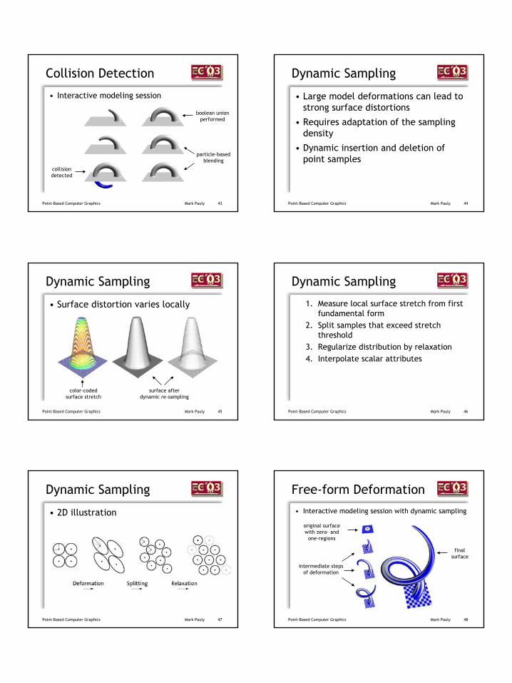
8
43Point-Based Computer Graphics Mark Pauly
Collision Detection
collisiondetected
boolean unionperformed
particle-basedblending
• Interactive modeling session
44Point-Based Computer Graphics Mark Pauly
Dynamic Sampling
• Large model deformations can lead to strong surface distortions
• Requires adaptation of the sampling density
• Dynamic insertion and deletion of point samples
45Point-Based Computer Graphics Mark Pauly
Dynamic Sampling
• Surface distortion varies locally
color-codedsurface stretch
surface afterdynamic re-sampling
46Point-Based Computer Graphics Mark Pauly
Dynamic Sampling
1. Measure local surface stretch from first fundamental form
2. Split samples that exceed stretch threshold
3. Regularize distribution by relaxation4. Interpolate scalar attributes
47Point-Based Computer Graphics Mark Pauly
Dynamic Sampling
• 2D illustration
48Point-Based Computer Graphics Mark Pauly
Free-form Deformation
• Interactive modeling session with dynamic sampling
original surfacewith zero- and
one-regions
intermediate stepsof deformation
finalsurface
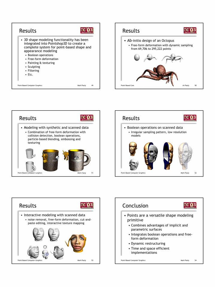
9
49Point-Based Computer Graphics Mark Pauly
Results
• 3D shape modeling functionality has been integrated into Pointshop3D to create a complete system for point-based shape and appearance modeling• Boolean operations• Free-form deformation• Painting & texturing• Sculpting• Filtering• Etc.
50Point-Based Computer Graphics Mark Pauly
Results
• Ab-initio design of an Octopus• Free-form deformation with dynamic sampling
from 69,706 to 295,222 points
51Point-Based Computer Graphics Mark Pauly
Results
• Modeling with synthetic and scanned data• Combination of free-form deformation with
collision detection, boolean operations, particle-based blending, embossing and texturing
52Point-Based Computer Graphics Mark Pauly
Results
• Boolean operations on scanned data• Irregular sampling pattern, low resolution
models
53Point-Based Computer Graphics Mark Pauly
Results
• Interactive modeling with scanned data• noise removal, free-form deformation, cut-and-
paste editing, interactive texture mapping
54Point-Based Computer Graphics Mark Pauly
Conclusion
• Points are a versatile shape modeling primitive• Combines advantages of implicit and
parametric surfaces• Integrates boolean operations and free-
form deformation• Dynamic restructuring• Time and space efficient
implementations

10
55Point-Based Computer Graphics Mark Pauly
Conclusion
• Complete and versatile point-based 3D shape and appearance modeling system• Directly applicable to scanned data • Suitable for low-cost 3D content creation
and rapid proto-typing
56Point-Based Computer Graphics Mark Pauly
References• Pauly: Point Primitives for Interactive Modeling and
Processing of 3D Geometry, PhD Thesis, ETH Zurich, 2003• Pauly, Keiser, Kobbelt, Gross: Shape Modeling with Point-
sampled Geometry, SIGGRAPH 03• Pauly, Kobbelt, Gross: Multiresolution Modeling with Point-
sampled Geometry, ETH Technical Report, 2002• Zwicker, Pauly, Knoll, Gross: Pointshop3D: An Interactive
System for Point-based Surface Editing, SIGGRAPH 02• Adams, Dutre: Boolean Operations on Surfel-Bounded Solids,
SIGGRAPH 03• Szeliski, Tonnesen: Surface Modeling with Oriented Particle
Systems, SIGGRAPH 92• www.pointshop3d.com


![CorelDRAW Graphics Suite 2019 - product.corel.comproduct.corel.com/.../CorelDRAW/...Guide/CorelDRAW-Graphics-Suite-2019.pdf · Schnellstarthandbuch [ 1 ] CorelDRAW Graphics Suite](https://img.pdfslide.tips/doc/110x75/5e0e571ce184e06f630a9a34/coreldraw-graphics-suite-2019-schnellstarthandbuch-1-coreldraw-graphics-suite.jpg)