Post-Hartree-Fock Wave Function Theory

Electron Correlation and Configuration Interaction

Video IV.ii

Electron Correlation How Important is It?

fi =− 1

2∇i2 –

Zkrikk

nuclei∑ + Vi

HF j{ }

The fundamental approximation of the Hartree-Fock method: interactions between electrons are treated in an average way, not an instantaneous way

H

One electron EHF = –0.500 00 a.u. Eexact = –0.500 00 a.u.

He

Two electrons EHF = –2.861 68 a.u. Eexact = –2.903 72 a.u. Error ~ 26 kcal mol–1 !

Infinite basis set results

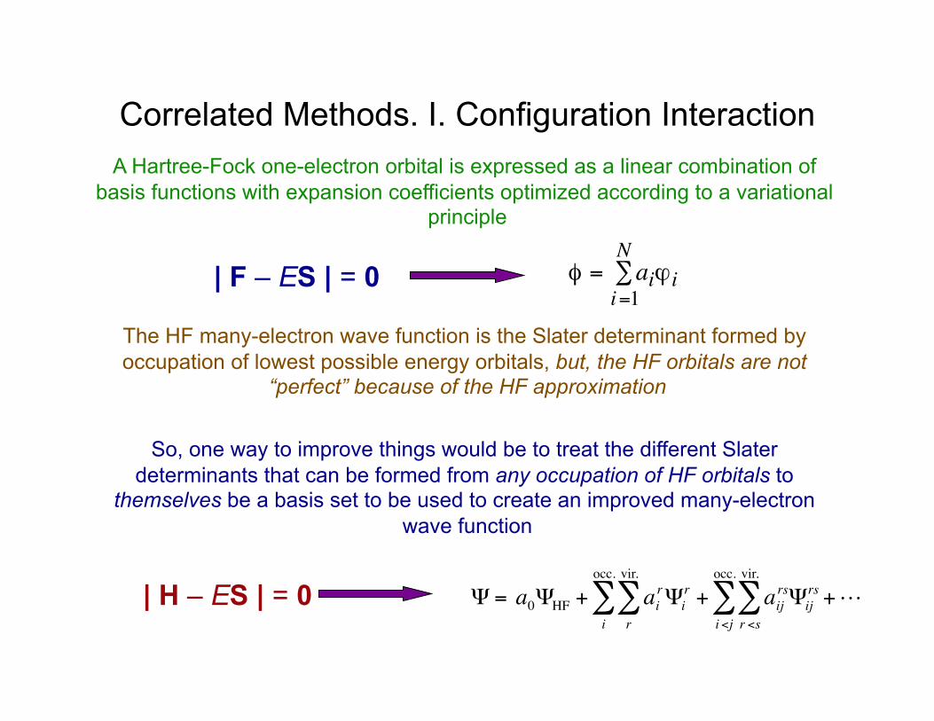
Correlated Methods. I. Configuration Interaction A Hartree-Fock one-electron orbital is expressed as a linear combination of

basis functions with expansion coefficients optimized according to a variational principle

| F – ES | = 0 φ = aiϕii=1

N∑

The HF many-electron wave function is the Slater determinant formed by occupation of lowest possible energy orbitals, but, the HF orbitals are not

“perfect” because of the HF approximation

So, one way to improve things would be to treat the different Slater determinants that can be formed from any occupation of HF orbitals to

themselves be a basis set to be used to create an improved many-electron wave function

| H – ES | = 0

€

Ψ = a0ΨHF + airΨi

r

r

vir.

∑i

occ.

∑ + aijrsΨij

rs

r <s

vir.

∑i<j

occ.

∑ +

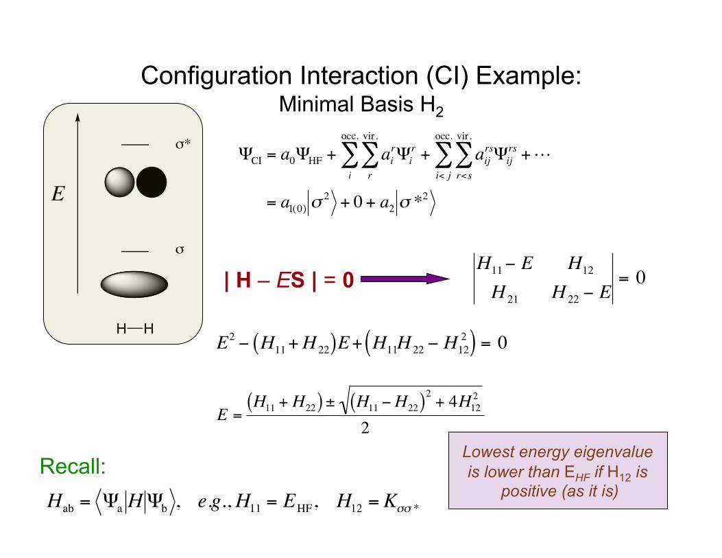
Configuration Interaction (CI) Example: Minimal Basis H2

| H – ES | = 0

€

ΨCI = a0ΨHF + airΨi

r

r

vir.

∑i

occ.

∑ + aijrsΨij

rs

r<s

vir.

∑i< j

occ.

∑ +

= a1(0) σ2 + 0 + a2 σ *

2E

H H

σ

σ*

€

H11− E H12

H 21 H 22 − E= 0

Recall:

€

Hab = Ψa HΨb , e.g.,H11 = EHF, H12 = Kσσ *

€

E2 − H11+H 22( )E+ H11H 22 − H122( ) = 0

€

E =H11 + H22( ) ± H11 −H22( )2 + 4H12

2

2Lowest energy eigenvalue is lower than EHF if H12 is

positive (as it is)

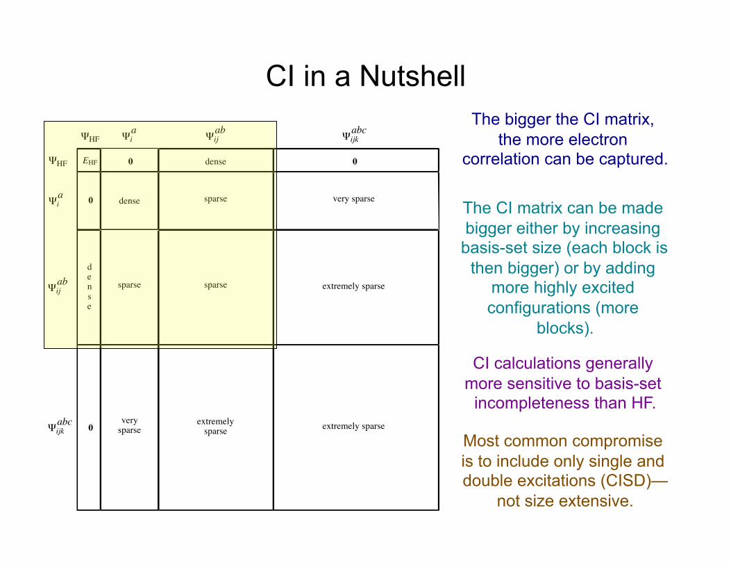
CI in a Nutshell

EHF 0

0

0

0dense

dense

sparse

sparse

extremelysparse

dense

sparse

verysparse

very sparse

extremely sparse

extremely sparse

ΨHF

ΨHF

Ψia

Ψia

Ψijab

Ψijkabc

Ψijab

Ψijkabc

The bigger the CI matrix, the more electron

correlation can be captured.

The CI matrix can be made bigger either by increasing basis-set size (each block is

then bigger) or by adding more highly excited configurations (more

blocks).

CI calculations generally more sensitive to basis-set

incompleteness than HF.

Most common compromise is to include only single and double excitations (CISD)—

not size extensive.

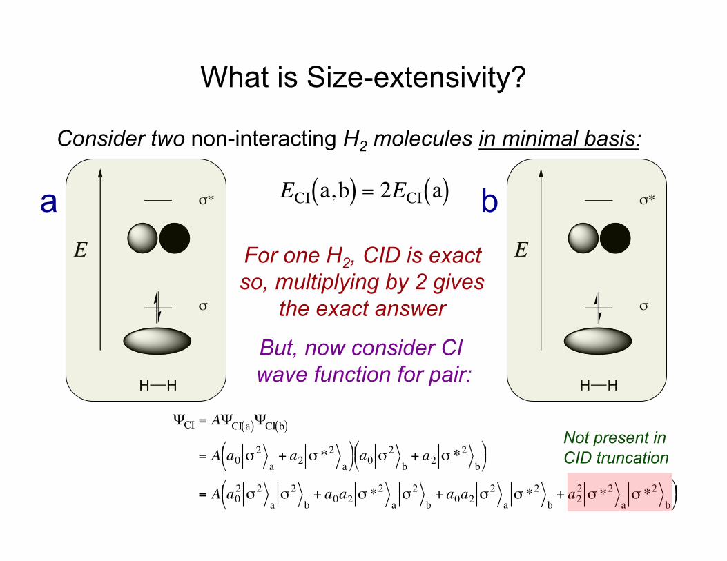
What is Size-extensivity?

Consider two non-interacting H2 molecules in minimal basis:

E

H H

σ

σ*

E

H H

σ

σ*

€

ΨCI = AΨCI a( )ΨCI b( )

= A a0 σ2a

+ a2 σ *2a

⎛ ⎝ ⎜ ⎞

⎠ ⎟ a0 σ

2b

+ a2 σ *2b

⎛ ⎝ ⎜ ⎞

⎠ ⎟

= A a02 σ2

aσ2

b+ a0a2 σ *

2aσ2

b+ a0a2 σ

2aσ *2

b+ a2

2 σ *2aσ *2

b

⎛ ⎝ ⎜ ⎞

⎠ ⎟

a b

€

ECI a,b( ) = 2ECI a( )

For one H2, CID is exact so, multiplying by 2 gives

the exact answer

But, now consider CI wave function for pair:

Not present in CID truncation

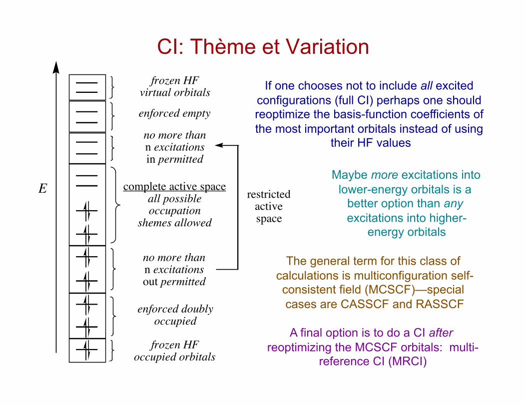
CI: Thème et Variation

If one chooses not to include all excited configurations (full CI) perhaps one should reoptimize the basis-function coefficients of the most important orbitals instead of using

their HF values

Maybe more excitations into lower-energy orbitals is a

better option than any excitations into higher-

energy orbitals

The general term for this class of calculations is multiconfiguration self-consistent field (MCSCF)—special cases are CASSCF and RASSCF

E complete active spaceall possibleoccupation

shemes allowed

no more thann excitationsout permitted

no more thann excitationsin permitted

frozen HFoccupied orbitals

enforced doublyoccupied

frozen HFvirtual orbitals

restrictedactivespace

enforced empty

A final option is to do a CI after reoptimizing the MCSCF orbitals: multi-

reference CI (MRCI)

Conceptual Test

If you compare the geometry of a molecule computed at the Hartree-Fock level compared to the same molecule computed at the CI level, in general, do you expect the bond lengths at the CI level to be longer or shorter than those at the HF level?

Explain your reasoning.

Post-Hartree-Fock Wave Function Theory

Perturbation Theory and Coupled-Cluster Theory

Video IV.iii

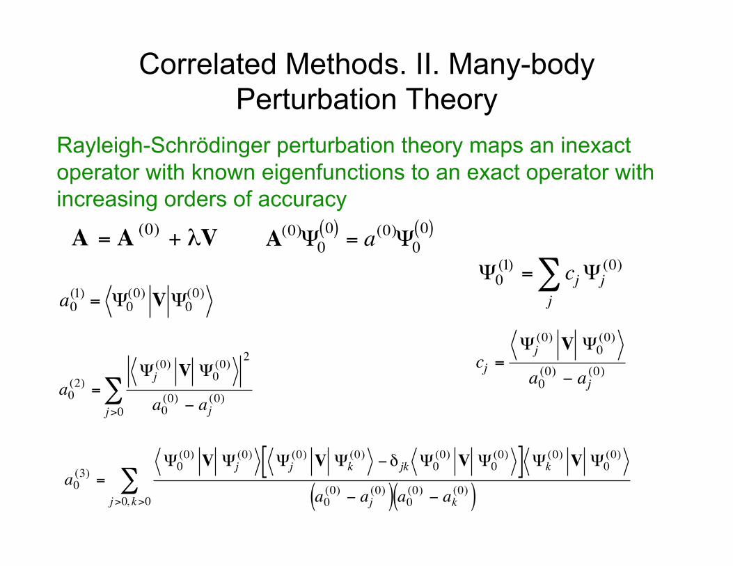
Correlated Methods. II. Many-body Perturbation Theory

Rayleigh-Schrödinger perturbation theory maps an inexact operator with known eigenfunctions to an exact operator with increasing orders of accuracy

€

A = A (0) + λV

€

Ψ0(1) = cjΨj

(0)

j∑

€

cj =Ψj(0) V Ψ0

(0)

a0(0) − aj

(0)

€

a0(1) = Ψ0

(0) V Ψ0(0)

€

a0(2) =

Ψj(0) V Ψ0

(0) 2

a0(0) − aj

(0)j>0∑

€

a0(3) =

Ψ0(0) V Ψj

(0) Ψj(0) V Ψk

(0) −δ jk Ψ0(0) V Ψ0

(0)[ ] Ψk(0) V Ψ0

(0)

a0(0) − aj

(0)( ) a0(0) − ak(0)( )j>0, k>0∑

€

A(0)Ψ00( ) = a(0)Ψ0

0( )

Møller-Plesset (MP) Perturbation Theory

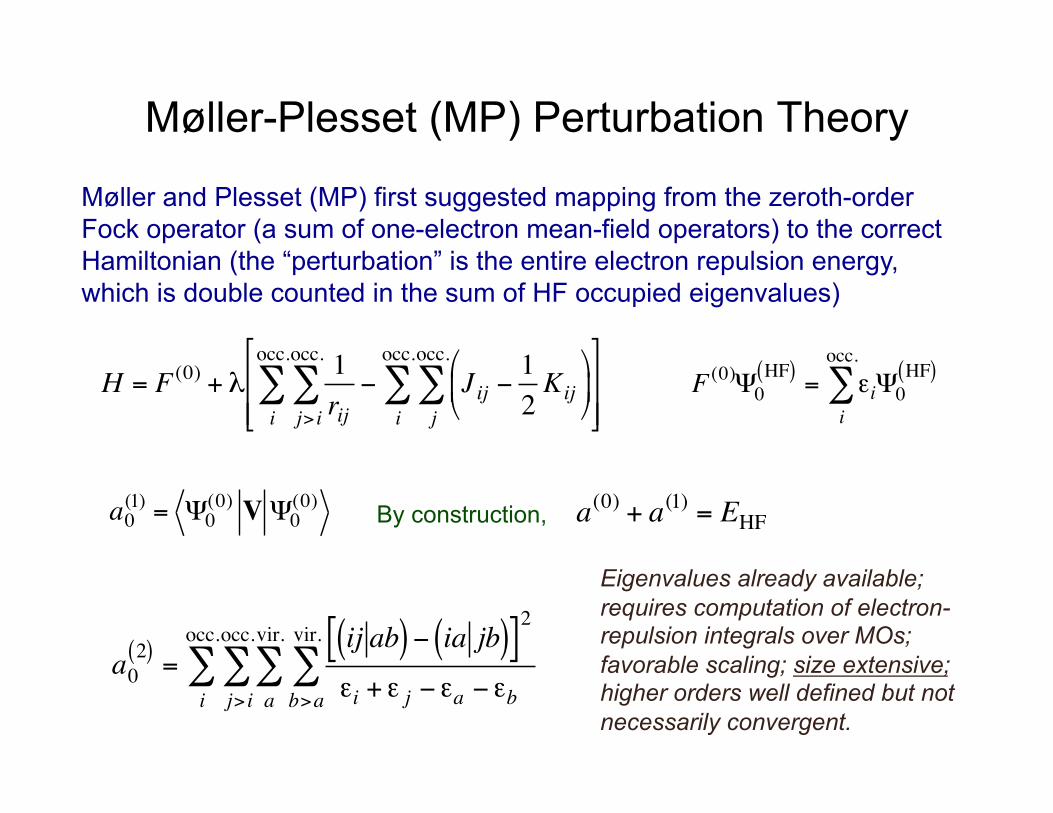
Møller and Plesset (MP) first suggested mapping from the zeroth-order Fock operator (a sum of one-electron mean-field operators) to the correct Hamiltonian (the “perturbation” is the entire electron repulsion energy, which is double counted in the sum of HF occupied eigenvalues)

€

H = F (0) + λ1rijj> i

occ.

∑i

occ.

∑ − Jij −12Kij

⎛

⎝ ⎜

⎞

⎠ ⎟

j

occ.

∑i

occ.

∑⎡

⎣ ⎢ ⎢

⎤

⎦ ⎥ ⎥

€

a0(1) = Ψ0

(0) V Ψ0(0)

€

F (0)Ψ0HF( ) = εi

i

occ.

∑ Ψ0HF( )

By construction,

€

a(0) + a(1) = EHF

€

a02( ) =

ij ab( ) − ia jb( )[ ]2

εi + ε j − εa − εbb>a

vir.

∑a

vir.

∑j> i

occ.

∑i

occ.

∑

Eigenvalues already available; requires computation of electron-repulsion integrals over MOs; favorable scaling; size extensive; higher orders well defined but not necessarily convergent.

Correlated Methods. II. Many-body Perturbation Theory

•  Rayleigh-Schrödinger perturbation theory maps an inexact operator with known eigenfunctions to an exact operator with increasing orders of accuracy

•  Møller and Plesset (MP) first suggested mapping from the zeroth-order Fock operator to the correct Hamiltonian (the “perturbation” is the entire electron repulsion energy…)

•  MP0 double-counts electron repulsion, MP1 = HF, MP2 captures a “good” amount of correlation energy at low cost, higher orders available (up to about MP6 in modern codes—becomes expensive rapidly)

•  Multireference options available: CASPT2, RASPT2, and analogs

•  No guarantee of convergent behavior—pathological cases occur with unpleasant frequency

Correlated Methods. III. Coupled Cluster CI adopts a linear ansatz to improve upon the HF reference

Coupled cluster proceeds from the idea that accouting for the interaction of one electron with more than a single other electron is unlikely to be important. Thus, to the extent that “many-electron” interactions are important, it will be through

simultaneous pair interactions, or so-called “disconnected clusters” An exponential ansatz can accomplish this in an elegant way. If we define

excitation operators, e.g., the double excitation operator as

€

Ψ = a0ΨHF + airΨi

r

r

vir.

∑i

occ.

∑ + aijrsΨij

rs

r <s

vir.

∑i<j

occ.

∑ +

€

T2ΨHF = tijab

a<b

vir.

∑i< j

occ.

∑ Ψijab

Then the full CI wave function for n electrons can be generated from the action of 1 + T = 1 + T1 + T2 + • • • + Tn on the HF reference

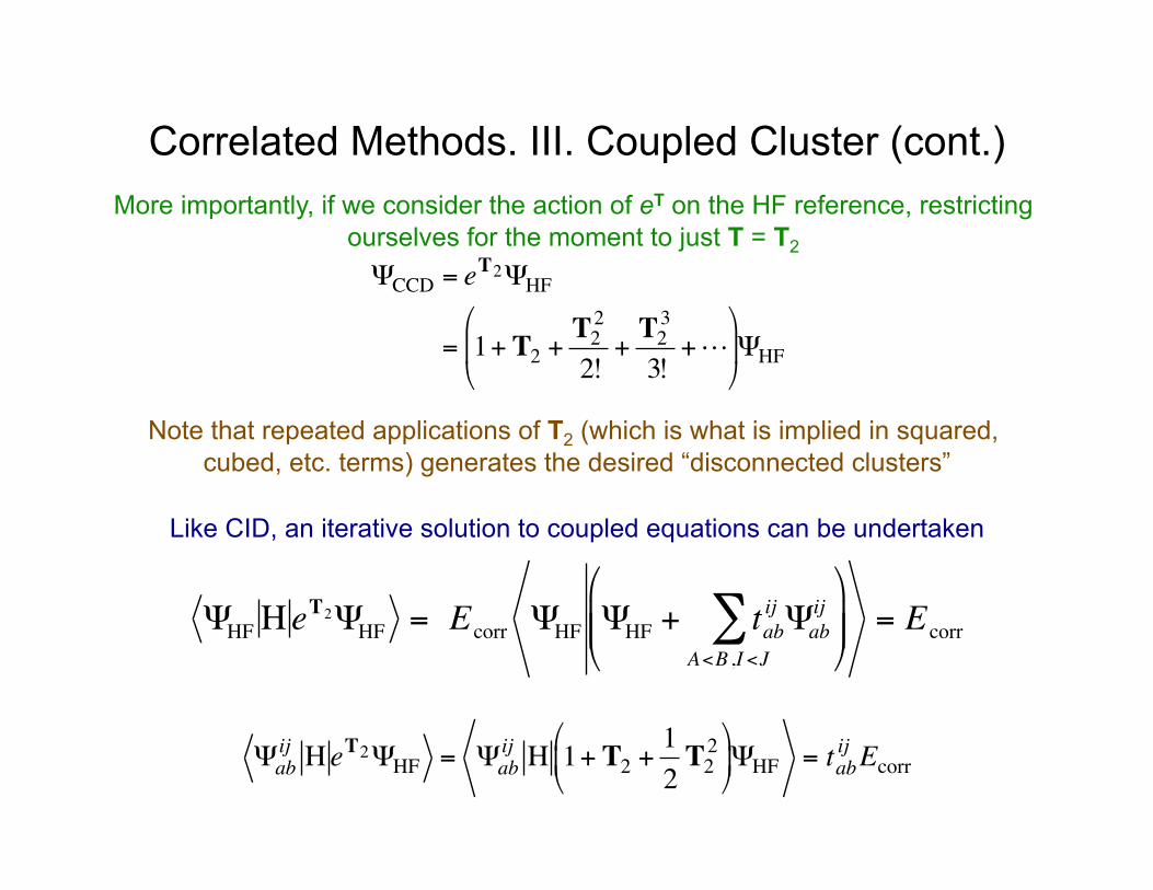
Correlated Methods. III. Coupled Cluster (cont.) More importantly, if we consider the action of eT on the HF reference, restricting

ourselves for the moment to just T = T2

Note that repeated applications of T2 (which is what is implied in squared, cubed, etc. terms) generates the desired “disconnected clusters”

Like CID, an iterative solution to coupled equations can be undertaken

€

ΨCCD = eT2ΨHF

= 1+ T2 +T22

2!+T23

3!+

⎛

⎝ ⎜

⎞

⎠ ⎟ ΨHF

€

ΨHFΗ eT2ΨHF = Ecorr ΨHF ΨHF + tab

ij Ψabij

A<B ,I <J∑

⎛

⎝ ⎜ ⎜

⎞

⎠ ⎟ ⎟ = Ecorr

€

Ψabij Η eT2ΨHF = Ψab

ij Η 1+ T2 +12T22⎛

⎝ ⎜

⎞

⎠ ⎟ ΨHF = tab

ij Ecorr

Correlated Methods. III. Coupled Cluster (cont.) The math is somewhat tedious, but the CC equations can be shown to be size-

extensive for any level of excitation

CCSD (single and double excitations) is convenient but addition of disconnected triples (CCSDT) is very expensive. A perturbative estimate of the effect of triple excitations defines the CCSD(T) method, sometimes called the “gold standard”

of modern single-reference WFT

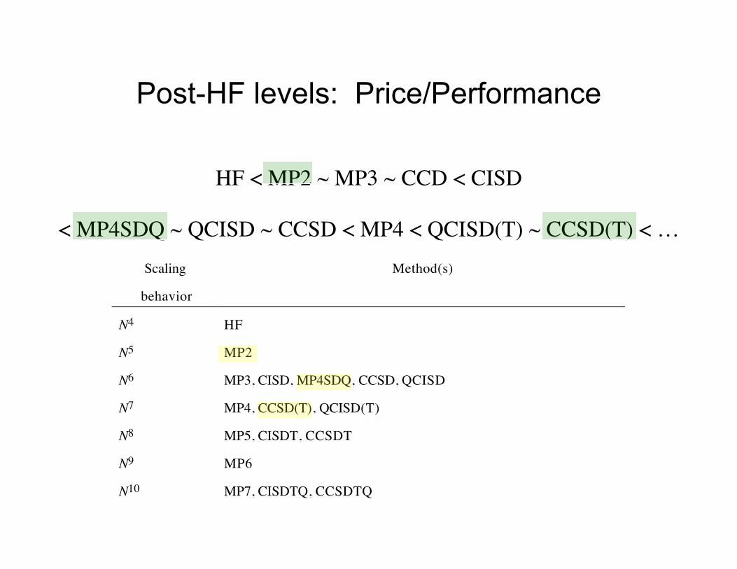
Post-HF levels: Price/Performance

HF < MP2 ~ MP3 ~ CCD < CISD

< MP4SDQ ~ QCISD ~ CCSD < MP4 < QCISD(T) ~ CCSD(T) < … Scaling

behavior

Method(s)

N4 HF

N5 MP2

N6 MP3, CISD, MP4SDQ, CCSD, QCISD

N7 MP4, CCSD(T), QCISD(T)

N8 MP5, CISDT, CCSDT

N9 MP6

N10 MP7, CISDTQ, CCSDTQ

From Electronic Energies to Thermodynamics

The Triumph of Statistical Mechanics (The Ideal-Gas, Rigid-Rotator,

Quantum-Mechanical-Harmonic-Oscillator Approximation)

Video IV.iv

How Does an Electronic Energy Relate to a Thermodynamic Quantity?

•  Electronic energies are unspeakably tiny energies referring to the potential energy of a single molecule at 0 K characterized by classical nuclei (only the electrons are treated quantum mechanically)

•  Chemistry involves an unspeakably large number of molecules whose distribution is governed by Boltzmann statistics at equilibrium

•  Thermodynamic quantities describe the ensemble properties of large numbers of molecules

•  One molecule at 0 K is like a ball on a PES, one mole of molecules at non-zero T is like a dense flock of birds, thinning in all directions from a central point, hovering above that surface and in constant motion with individual birds going up, down, back, and forth…

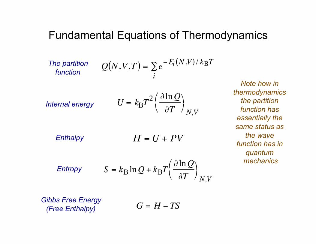
Fundamental Equations of Thermodynamics

Q N ,V,T( ) = e−Ei N ,V( ) / kBT

i∑

U = kBT2 ∂ lnQ

∂T⎛ ⎝

⎞ ⎠ N,V

H =U + PV

S = kBlnQ + kBT∂ lnQ∂T

⎛ ⎝

⎞ ⎠ N,V

G = H − TS

The partition function

Internal energy

Enthalpy

Entropy

Gibbs Free Energy (Free Enthalpy)

Note how in thermodynamics

the partition function has

essentially the same status as

the wave function has in

quantum mechanics

A Convenient Partition Function

Q N ,V,T( ) = e−Ei N ,V( ) / kBT

i∑The partition

function

Identifying all possible energy states available to an arbitrary system is a brobdingnagian task. A simplification is to take the system to be an ideal gas. By definition, the individual molecules of the ideal gas do not interact with one another, so the total energy is the sum of

their individual energies:

Q N ,V,T( ) =1N!

e− ε1 V( )+ε2 V( )++εN V( )[ ]i / kBT

i∑

=1N!

e−ε j 1( ) V( ) / kBT

j 1( )∑

⎡

⎣ ⎢

⎤

⎦ ⎥ e

−ε j 2( ) V( ) / kBT

j 2( )∑

⎡

⎣ ⎢

⎤

⎦ ⎥ e

−ε j N( ) V( ) /kBT

j N( )∑

⎡

⎣ ⎢

⎤

⎦ ⎥

=1N!

gke−εk V( ) / kBT

k

levels∑

⎡

⎣ ⎢ ⎤

⎦ ⎥

N

=q V,T( )[ ]N

N!

The sum

Exponential of sum is product of exponentials

All molecules of ideal gas are identical

q is molecular partition function

What Contributes to the Total Energy of a Molecule?

Electronic energy: (from Schrödinger or Kohn-Sham eqs)

Translational kinetic energy: (dense levels, like classical system; depends only on molecular weight, choice of standard-

state volume, and temperature; 0 at 0 K)

Rotational kinetic energy: (if rigid rotator: dense levels, like classical system; depends only on principal moments of inertia

and temperature; 0 at 0 K)

Vibrational kinetic energy: (if harmonic oscillator: not dense levels, but convergent sum; depends only on

molecular vibrational frequencies (normal modes) and temperature;

not 0 at 0 K for QMHO)

Zero-point vibrational energy (ZPVE)

Practical thermodynamic calculations require only that a geometry and vibrational frequencies be available

How to Reconcile Experimental and Theoretical Standard-State Conventions?

Elemental Standard States0.0

Ener

gy U

nits

spin-orbitcorrected

atomiccalculations

molecularcalculations

ΔGof,298ΔHo

f,298ΔHof,0

+ZPVE

+(H298–H0) –298So298

+(H298–H0)–298So

298

Com

pute

d Δ

E

Com

pute

d Δ

H0

Com

pute

d Δ

H29

8

Com

pute

d Δ

Go 29

8

atomicexperimental

data

atomization energy

Conceptual Test

Calculations at semiempirical levels of theory report heats of formation without ever doing frequency calculations. Explain how the predicted heat of formation is computed and what is involved in foregoing a frequency calculation.

How ‘bout Those Post-HF WFTs?

Benchmarking the Models

Video IV.v

Post-HF levels: Price/Performance

HF < MP2 ~ MP3 ~ CCD < CISD

< MP4SDQ ~ QCISD ~ CCSD < MP4 < QCISD(T) ~ CCSD(T) < … Scaling

behavior

Method(s)

N4 HF

N5 MP2

N6 MP3, CISD, MP4SDQ, CCSD, QCISD

N7 MP4, CCSD(T), QCISD(T)

N8 MP5, CISDT, CCSDT

N9 MP6

N10 MP7, CISDTQ, CCSDTQ

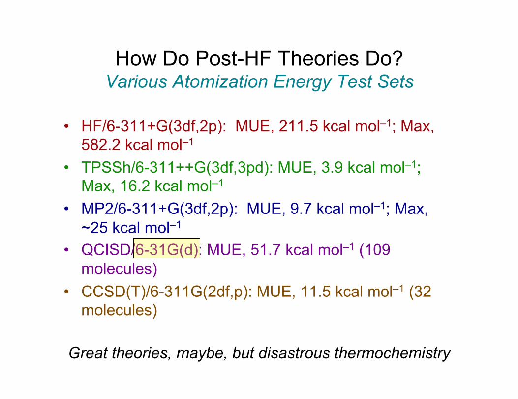
How Do Post-HF Theories Do? Various Atomization Energy Test Sets

•  HF/6-311+G(3df,2p): MUE, 211.5 kcal mol–1; Max, 582.2 kcal mol–1

•  TPSSh/6-311++G(3df,3pd): MUE, 3.9 kcal mol–1; Max, 16.2 kcal mol–1

•  MP2/6-311+G(3df,2p): MUE, 9.7 kcal mol–1; Max, ~25 kcal mol–1

•  QCISD/6-31G(d): MUE, 51.7 kcal mol–1 (109 molecules)

•  CCSD(T)/6-311G(2df,p): MUE, 11.5 kcal mol–1 (32 molecules)

Great theories, maybe, but disastrous thermochemistry

Correlated Methods. IV. Multilevel Protocols

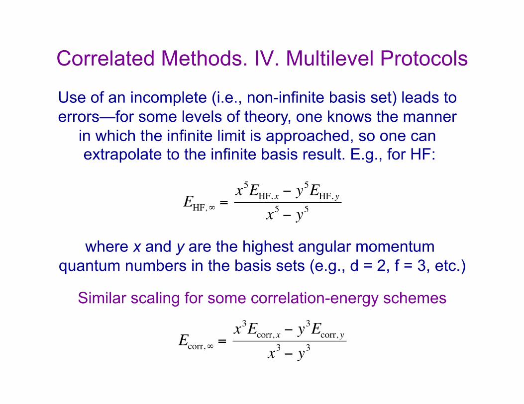
Use of an incomplete (i.e., non-infinite basis set) leads to errors—for some levels of theory, one knows the manner

in which the infinite limit is approached, so one can extrapolate to the infinite basis result. E.g., for HF:

€

EHF,∞ =x5EHF, x − y

5EHF, yx5 − y5

where x and y are the highest angular momentum quantum numbers in the basis sets (e.g., d = 2, f = 3, etc.)

Similar scaling for some correlation-energy schemes

€

Ecorr,∞ =x3Ecorr, x − y

3Ecorr, yx3 − y3

Multilevel Protocols: Tema y Variación

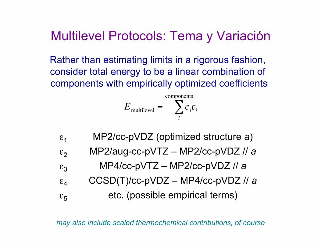
Rather than estimating limits in a rigorous fashion, consider total energy to be a linear combination of components with empirically optimized coefficients

€

Emultilevel = ciεii

components

∑

ε1 MP2/cc-pVDZ (optimized structure a) ε2 MP2/aug-cc-pVTZ – MP2/cc-pVDZ // a ε3 MP4/cc-pVTZ – MP2/cc-pVDZ // a ε4 CCSD(T)/cc-pVDZ – MP4/cc-pVDZ // a ε5 etc. (possible empirical terms)

may also include scaled thermochemical contributions, of course

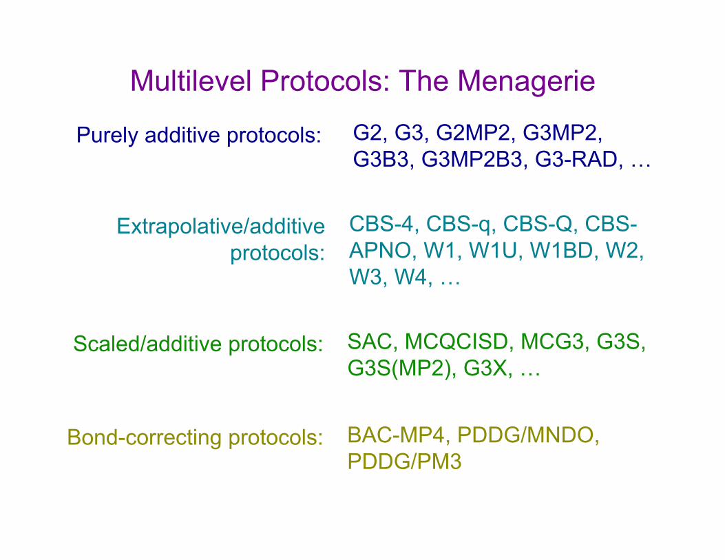
Multilevel Protocols: The Menagerie

Purely additive protocols: G2, G3, G2MP2, G3MP2, G3B3, G3MP2B3, G3-RAD, …

Extrapolative/additive protocols:

CBS-4, CBS-q, CBS-Q, CBS-APNO, W1, W1U, W1BD, W2, W3, W4, …

Scaled/additive protocols: SAC, MCQCISD, MCG3, G3S, G3S(MP2), G3X, …

Bond-correcting protocols: BAC-MP4, PDDG/MNDO, PDDG/PM3

How Do Multilevel Protocols Do? Various Atomization Energy Test Sets

•  HF/6-311+G(3df,2p): MUE, 211.5 kcal mol–1; Max, 582.2 kcal mol–1

•  MP2/6-311+G(3df,2p): MUE, 9.7 kcal mol–1; Max, ~25 kcal mol–1

•  CBS-Q: MUE, 1.2 kcal mol–1; Max, 8.1 kcal mol–1

•  G3: MUE, 1.1 kcal mol–1; Max, 7.1 kcal mol–1

•  W2: MUE, 0.5 kcal mol–1; Max, 1.9 kcal mol–1 (55 molecules—wildly expensive)

What’s the Right Way to Do a Calculation?

•  Solve the Schrödinger equation exactly (full CI, infinite basis)—rarely practical…

•  Use a multilevel approach to get as close as you can to the exact solution

•  Use an isodesmic protocol to foster error cancellation •  Assume error transferability between related known

and unknown systems at an affordable level •  Assume that good results for a known property of the

system will ensure good results for an unknown

•  Indulge in optimism and hope

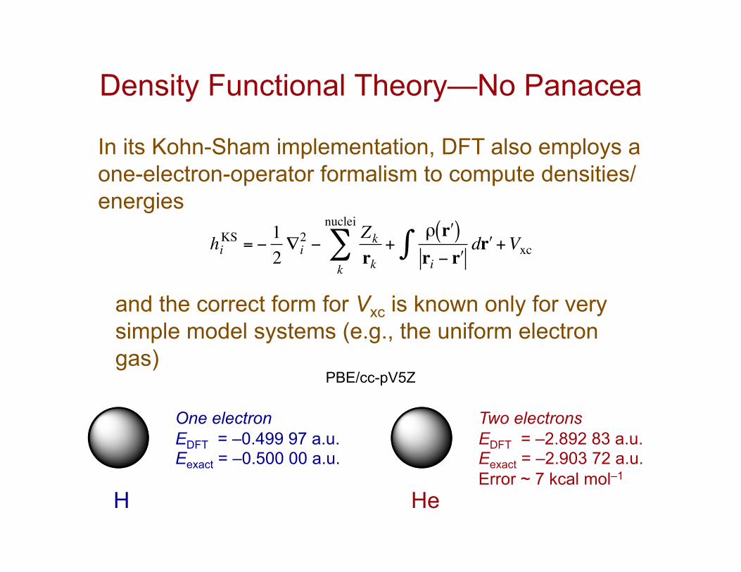
Density Functional Theory—No Panacea

In its Kohn-Sham implementation, DFT also employs a one-electron-operator formalism to compute densities/energies

€

hiKS = −

12∇i2 −

Zkrk

+ρ rʹ′( )ri − rʹ′

drʹ′+Vxc∫k

nuclei

∑

and the correct form for Vxc is known only for very simple model systems (e.g., the uniform electron gas)

H

One electron EDFT = –0.499 97 a.u. Eexact = –0.500 00 a.u.

He

Two electrons EDFT = –2.892 83 a.u. Eexact = –2.903 72 a.u. Error ~ 7 kcal mol–1

PBE/cc-pV5Z

What the Hell is Density Functional Theory?

Hohenberg and Kohn proved that the total energy can be determined exclusively from the electron density

€

E ρ r( )[ ] =T ρ r( )[ ] +V ρ r( )[ ]

conceptually simple but operationally challenging! In practice one employs

€

E ρ r( )[ ] =T ρ * r( )[ ] −ρ r( )Zkr − rk

dr∫k

nuclei

∑ +12

ρ r( )ρ ʹ′ r ( )r − ʹ′ r

drd ʹ′ r +∫∫ Vxc ρ r( )[ ]

where ρ* is the correct density but for non-interacting electrons and Vxc corrects for this approximation and using the classical repulsion energy

How Do One-electron Theories Do? G3/99 Test Set (223 Molecules)

•  HF/6-311+G(3df,2p): MUE, 211.5 kcal mol–1; Max, 582.2 kcal mol–1

•  LDA/6-311+G(2df,p): MUE, 121.9 kcal mol–1; Max, 347.5 kcal mol–1

•  BPW91/6-311++G(3df,3pd): MUE, 9.0 kcal mol–1; Max, 28.0 kcal mol–1

•  TPSS/6-311++G(3df,3pd): MUE, 5.8 kcal mol–1; Max, 22.9 kcal mol–1

•  TPSSh/6-311++G(3df,3pd): MUE, 3.9 kcal mol–1; Max, 16.2 kcal mol–1

Hybrid DFT not bad, but still not really acceptable