PRESSURE DROP MEASUREMENT FOR

SINGLE AND TWO-PHASE FLOWS IN

HORIZONTAL MICRO-FIN TUBES

Paloma Vega-Penichet Domecq paloma.vega-penichetd@alumnos.upm.es

1

“Soy de las que piensan que la ciencia tiene una gran belleza. Un científico en su laboratorio no es solo un técnico: también es un niño colocado ante fenómenos naturales que lo impresionan como un cuento de hadas”

- Marie Curie

Esta tesis esta dedicada a Mi Ni.

2

3

Después de cuatro intensos años acaba esta etapa, aunque solo sea para empezar una nueva. Este logro nunca hubiera llegado de no haber sido por las personas que me han rodeado durante este tiempo. Para empezar, mi queridísimo tutor Luigi Colombo, que no solo me ha enseñado en el ámbito intelectual, sino en el humano, aprendiendo de él, que aún cuando parece que no hay fuerzas, siempre queda un último aliento para una sonrisa. También mi cotutor, Rubén Abbas, que con miles de kilómetros de por medio, siempre ha estado atento. Mi familia, que ha aguantado mis peores momentos de agotamiento. Mis amigas, que siempre han sabido robarme un segundo, incluso cuando creía que no tenerlo. Y todos aquellos que han hecho que la universidad sea como una segunda casa, y no por el tiempo que hemos pasado en ella, que si por eso fuese sería la primera, sino por los ánimos que siempre me han dado.

Gracias a todos, por que no estaría donde estoy si no fuera por vosotros.

4

5

RESUMEN Esta tesis tiene como objetivo el estudio de la caída de presión dentro de dos tipos de tubos, liso y micro-aleteado, con el fin de comparar los resultados obtenidos en ambos.

A día de hoy, el rendimiento es un aspecto muy importante en todos los campos. Es por esta razón por la que nace el tubo micro-aleteado, con el fin de mejorar la eficiencia en el intercambio de calor. Este tipo de tubo tiene las siguientes características: una mayor superficie de intercambio de calor gracias a las micro-aletas que aparecen adheridas a su superficie y un incremento de los distintos mecanismos de intercambio de calor como, promover turbulencia y humectabilidad de la pared, comparado con el tubo liso .

Con el crecimiento del coeficiente de transferencia de calor viene a su vez un incremento en la caída de presión. Por ello, es conveniente definir un coeficiente de mejora de la transferencia de calor y un factor de penalización para la caída de presión. Así, los dos factores serán comparados para entender cuál es la configuración óptima en términos de: altura, forma y número y, finalmente, escoger el tubo adecuado.

Este trabajo se basa en la evaluación del factor de penalización por medio de una caracterización experimental que incluye el flujo adiabático agua-aire. La literatura ha comprobado que estas condiciones de operación son también adecuadas para la determinación de la caída de presión en flujos con intercambio de calor aire-agua. De todas formas, el sistema experimental relacionado con el primero es mucho más simple que el requerido para el segundo. Por ello, es de gran interés el estudio de los flujos adiabáticos, ya que aceleran el proceso de recogida de datos, puesto que, como se ha dicho, el sistema es mucho más simple y por lo tanto más fácil de manejar.

TABLA R1. Datos geométricos de el tubo liso y el tubo micro-aleteado.

Smooth tube L = 1.295 m d = 0.00892 m

Micro-fin tube Internal diameter (di) = 0.00892 m External diameter (de) = 0.0095 m

L = 1.298 m Cross section area (W) = 61.72 mm2

Wet perimeter = 39.9 mm2 Fin type 1 Fin type 2

Number (n) = 27 Number (n) = Height (h) = 0.16 mm Height (h)= 0.23 mm

Fin angle (g) = 40º Fin angle (g) = 40º Helix angle (b) = 18º Helix angle (b) = 18º

6

En esta tesis, se usarán dos tubos, ambos de cobre, uno liso y otro tubo micro-aleteado que tiene aleteada la superficie interior, contando con aletas intercaladas de dos tamaños, que siguen una curva helicoidal. Los datos relacionados con la geometría de ambos tubos son presentados en la Tabla R1.

El montaje experimental (Representado en la Figura R1) está compuesto por dos circuitos: agua y aire, que permiten el flujo monofásico de agua y el bifásico aire-agua que recorreran un camino compuesto por una sección de mezcla (Mixing section) , una sección de prueba (Test section) y una sección de visualización (Visualization section). Por último, el flujo se descarga en el tanque de agua, donde el aire se separa del agua y es expulsado al ambiente.

En la sección de mezcla los flujos de agua y aire se unen y recorren el camino necesario para estabilizar el flujo bifásico.

Después, en la sección de prueba, se encuentra el transductor de presión diferencial (DPT, Diferenctial Pressure Transducer), que es el encargado de tomar las presiones a la entrada y a la salida del tubo de prueba y enviarlas a la unidad de adquisición de datos (DAU, Data Acquisition Unit), que proporcionará los datos recogidos permitiendo así obtener la diferencia de presión en el tubo debida a la fricción. Esto se consigue gracias a una válvula de tres vías conectada al transductor de forma que, para una posición de la válvula el transductor recoge la presión aguas arriba y para la otra la recoge aguas abajo.

Finalmente, a la salida de la sección de prueba se encuentra una sección de visualización compuesta por un tubo horizontal transparente que permite observar el tipo de flujo que tiene lugar.

FIGURA R1. Representación esquemática del sistema experimental del trabajo.

7

En cuanto a las condiciones de operación, estas han sido seleccionadas con la finalidad de obtener flujos turbulentos tanto en el flujo monofásico como en el bifásico, de forma que el flujo másico (G) y el título de vapor (x) quedan definidos en los rangos recogidos en la tabla R2. Además, el rango de operación está limitado por el transductor de presión diferencial, que tiene como máximo una medida relativa de presión de 70kPa.

TABLA R2. Condiciones de operación del experimento.

Definidas las condiciones, el siguiente paso es recoger los datos para los distintos tubos y los distintos flujos.

El procedimiento experimental es distinto para el flujo monofásico y para el bifásico. Pero dentro de un tipo de flujo el procedimiento es el mismo para los dos tipos de tubos.

Para empezar, el procedimiento experimental para el flujo monofásico de agua es el siguiente:

1. Inicio del sistema mediante la apertura de válvulas y la puesta en marcha del motor. 2. Regulación del caudal por medio del caudalímetro. 3. Toma de medidas. Una vez se ha estabilizado el flujo de agua dentro del tubo, se

observa el tipo de flujo a través de la sección de visualización, y se procede a la toma de las medidas. Para cada caudal han de tomarse las presiones a la entrada de la sección de prueba y a la salida. Recordar que esto se consigue por medio de la válvula de tres vías que conecta el tubo a estudiar con el transductor de presión. Además de la presión, se tomará también la temperatura del agua.

4. Variación de caudal. Se volverá al paso 2 estableciendo un nuevo caudal y tomando los datos para este, de forma que todo el rango de condiciones de operación quede cubierto.

5. Reiteración. Una vez el rango de operación queda cubierto se repite diez veces el proceso y así, para cada caudal fijado, existen 10 datos de caída de presión que serán promediados para reducir errores.

En cuanto al flujo bifásico, la complejidad aumenta, y el proceso es el siguiente:

1. Inicio del sistema. Primero se establecerá el flujo de agua, de la misma forma que para el flujo monofásico. Después, el circuito de aire es abierto y comienza así el flujo bifásico.

2. Regulación del caudal. En el flujo aire-agua la complejidad es mayor. Para ello se comienza con la regulación del agua, fijando el caudal con el caudalímetro. Después, se continua con la regulación del aire, se establece la presión del sistema (4 bar) y luego el caudal, teniendo en cuenta que la regulación del caudal de aire afecta a la

Monofásico Bifásico G [kg/(sm2)] G [kg/(sm2)] x [-]

Liso 220-1800 220-1800 0.012-0.515 Micro-aleteado 50-480 50-480 0.012-0.515

8

presión del mismo, por lo tanto se irán comprobando y reajustando estos dos parámetros hasta conseguir los valores deseados. Por último, se comprueba que el caudal del agua no haya variado y se reajusta si es necesario.

3. Toma de medidas. Una vez el flujo se ha estabilizado, se observa el tipo de flujo mediante la sección de visualización. Después se procede a la recolecta de datos. Para ello, como en el flujo monofásico, se hará uso de la válvula de tres vías para recoger presiones aguas arriba y aguas abajo del tubo.

4. Variación de caudal de aire. Lo siguiente es, manteniendo el caudal de agua, variar el caudal de aire de manera que se obtienen medidas para todo el rango de condiciones de operación del aire, para un caudal de agua determinado. Siempre tomando nota del tipo de flujo que se observa mediante la sección de visualización.

5. Variación de caudal de agua. Una vez el rango de condiciones de aire esta cubierto, se reinicia el proceso desde el paso 2, con un nuevo caudal de agua, y se repite cíclicamente hasta que el rango de condiciones de operación del agua quede cubierto.

6. Reiteración. Todo el proceso se repetirá cinco veces, de manera que para pareja de caudal de agua y caudal de aire existan cinco datos de diferencia de caída de presión, que de nuevo, serán promediados para reducir errores..

La recolecta de datos se comienza por el flujo de agua en el tubo liso, que se utiliza para la calibración del sistema, es decir, para fijar el diámetro interior del tubo. De los datos obtenidos, se puede decir que, puesto que los datos siguen con muy poca deviación las dos correlaciones estudiadas (Blasius y Petukhov [1] ), el diámetro proporcionado por el fabricante es el correcto y por lo tanto se mantiene ese valor.

Esto queda reflejado en la Figura R2, que representa el factor de fricción para las dos correlaciones elegidas de la literatura y el experimentalmente obtenido. En Tabla R3 se recogen la desviación media relativa (MRD) y la desviación media absoluta relativa (MARD), definidas como:

En la fórmula, el subíndice ‘pred’ hace referencia al factor de fricción predicho por el modelo (Blasius o Petukhov) mientras que, el subíndice ‘exp’ hace referencia al factor de fricción obtenido experimentalmente.

TABLA R3. MRD y MARD para las correlaciones usadas para la calibración.

𝑀𝑅𝐷 = %&Σ()%& *+,-./01*+,/2-

*+,/2- [%] (R1)

𝑀𝐴𝑅𝐷 = %&Σ()%& 5*+,-./01*+,/2-

*+,/2-5 [%] (R2)

MRD [%] MARD [%]

Blasius -0.512 3.217 Pethukov -0.713 4.192

9

FIGURA R2. Comparación del factor de fricción experimental con dos correlaciones.

Una vez calibrado el sistema, se procede a la recolección de datos para el flujo bifásico dentro del tubo liso y al procesamiento de los mismos para obtener una información más valiosa que la diferencia de presión, que se recuerda que es el dato obtenido mediante la unidad de adquisición de datos, para así poder comprar con distintas correlaciones de la literatura.

En este resumen se presentan únicamente unas breves conclusiones sobre las comparaciones.

Las correlaciones utilizadas para la comparación de los datos recogidos con el flujo bifásico en el tubo liso son: Chisholm [2], Sun and Mishima [3], Wang et al. [4], Muarata [5], Muller-Steinhagen and Heck [6], Tran et al. [7], McAdams , Chen et. Al. [8] and Shannak [9].

Estas correlaciones siguen 2 modelos distintos para el estudio de los flujos bifásicos. Estos modelos son:

1. Modelo de flujo homogéneo. 2. Modelo de flujos separados.

Existen correlaciones basadas en otros tipos de modelos , como por ejemplo, basados en el tipo de flujo (anular, neblina, ondulado…) pero, este tipo de correlaciones no se recogen en este trabajo.

Los resultados obtenidos tras el procesamiento de los datos quedan reflejados en la tabla R4 y las figuras R3, R4, R5, R6, R7, R8, R9, R10 y R11.

Para empezar, en la tabla quedan recogidas las desviaciones medias relativas (MRD) y las desviaciones medias absolutas relativas (MARD), que se presentaron en las ecuaciones R1 y R2.

Después, las figuras, recogen lo que se conoce como gráficas de paridad, en las que en el eje X se encuentran los datos recogidos experimentalmente y en el eje Y los datos obtenidos mediante las distintas correlaciones. A cada correlación utilizada se le asigna una gráfica distinta. Además, en estas gráficas se representan también la bisectriz y dos líneas de 20% de

10

desviación, positiva y negativa. Si los puntos aparecen por encima de la bisectriz esto quiere decir que el modelo sobrestima los datos experimentales, mientras que en el otro caso los subestima.

TABLA R4. Resultados de las comparaciones con las correlaciones para el tubo liso.

FIGURA R3. Gráfica de paridad de McAdams. FIGURA R4. Gráfica de paridad de Chen et. al.

FIGURA R5. Gráfica de paridad de Shannak. FIGURA R6. Gráfica de paridad de Chisholm.

Correlaciones tubo liso MRD% MARD% Chisholm 5.96 17.15 Sun and Mishima -36.81 36.81 Wang et al. -45.23 45.23 Murata -49.16 49.16 Muller Steinhagen and Heck 19.63 21.74 Tran et al. 54.04 54.04 McAdams 2.69 16.99 Chen et al. 85.34 85.34 Shannak 17.03 23.51

11

FIGURA R7. Gráfica de paridad de Sun and Mishima.

FIGURA R8. Gráfica de paridad de Wan et. al.

FIGURA R9. Gráfica de paridad de Murata. FIGURA R10. Gráfica de paridad de Muller-Steinhagen and Heck.

FIGURA R11. Gráfica de paridad de Tran et. al.

12

De los resultados se deduce que las mejores correlaciones para el flujo bifásico dentro del tubo liso, para las condiciones particulares de este trabajo son: McAdams y Chisholm. Seguidas por Shannak y Muller-Steinhagen and Heck.

También es interesante el comportamiento observado en la figura R9, asociada a la correlación de Murata, en la que se pueden distinguir dos ramas divergentes. La que más se acerca a la bisectriz, es decir, la que mejor sigue los datos experimentales, esta relacionada con los datos obtenidos para los flujos más pequeños es decir, de 50 kg/(sm2) a 270 kg/(sm2). Mientras que, la segunda rama, que ofrece una peor aproximación, esta relacionada con los datos tomados para flujos másicos entre 270 kg/(sm2) y 480 kg/(sm2). Por lo tanto, esta correlación será adecuada para flujos másicos bajos.

Una vez estudiado el comportamiento del tubo liso, se cambia este tubo por el micro-aleteado, que es montado en el sistema para llevar acabo su estudio.

De nuevo, se comienza por el flujo monofásico de agua, y una vez recogidos los datos se procesan para obtener la información necesaria.

Del flujo monofásico dentro del tubo micro-aleteado se obtiene una rugosidad relativa, que será después utilizada para la obtención de la caída de presión bifásica mediante la correlación de Shannak.

Esta rugosidad se obtiene comparando los datos experimentales con la correlación de Haaland, desarrollada para flujo monofásico en tubos rugosos [1]:

Donde 𝜀 𝐷⁄ hace referencia a la rugosidad relativa del tubo.

Para cada dato se obtiene la rugosidad relativa experimental y luego se realiza el promedio de las mismas. Como bien refleja la figura R12, los tres primeros datos no se tendrán en cuenta para el promedio puesto que no siguen la tendencia del resto, esto se debe a que para estos el flujo todavía no es anular sino flujo de tipo marea.

FIGURA R12. Factor de fricción experimental junto con la el factor de fricción de Haaland.

%89= −1.8𝑙𝑜𝑔 ABC D⁄

E.FG%.%%

+ I.JKLM;

13

La rugosidad relativa que se obtiene es e/D = 0.006863659 con una desviación estática de 0.001481.

Después del flujo monofásico en el tubo micro-aleteado, se estudia el flujo bifásico. Las correlaciones utilizadas para este tipo de flujo son: Shannak [9], Haraguchi [10], Kedzierski [11], Murata [5] y Cavallini [12].

Como para el tubo liso, se presentan los resultados obtenidos en la tabla R5 y se grafican en las figuras R13, R14, R15, R16 y R17.

Tabla R5. Resultados de las comparaciones con las correlaciones para el tubo micro-aleteado.

Figura R13. Diagrama de paridad de Shannak.

Figura R14. Diagrama de paridad de Haraguchi.

Figura R15. Diagrama de paridad de Kedzierski.

Figura R16. Diagrama de paridad de Murata.

Correlaciones MRD% MARD% Shannak 7.25 16.47 Haraguchi 21.37 29.79 Kedzierski -36.97 45.71 Murata -33.88 45.48 Cavallini -64.93 66.18

14

Figura R17. Diagrama de paridad Cavallini.

De las figuras y la tabla se puede deducir que la correlación que mejor se adapta a las condiciones particulares del trabajo para el tubo micro-aleteado es la de Shannak con la rugosidad relativa obtenida del flujo monofásico de agua.

Por último, se estudia el factor de penalización para los dos flujos, agua y aire-agua. En la figura R18 se observa como el factor de penalización del flujo monofásico se mantiene siempre por encima de este mismo para el flujo bifásico. Este resultado concuerda con el mejor rendimiento de los tubos micro-aleteados con el flujo bifásico.

Además, el factor de penalización para el flujo bifásico alcanza un valor mas o menos constante para flujos de masa mayores que 100 kg/(sm2) de forma que, promediando los valores a partir de los cuales se observa esa constancia, se obtiene un factor de penalización medio de valor 1,23. Mientras que, promediando de nuevo el factor de penalización, pero esta vez para el flujo de agua, el valor obtenido para el valor medio es de 1,326. Confirmando de nuevo, que el tubo micro-aleteado es más adecuada para el uso en flujos bifásicos.

Como se introdujo al principio, para la selección de la mejor opción de tubo micro-aleteado para un sistema determinado, se necesita estudiar el factor de penalización y el factor de mejora de la transferencia de calor. Este último factor si necesita el flujo con transferencia de calor y por lo tanto su obtención es más compleja.

Para concluir, decir que este tema y su ámbito necesitan mayor investigación. De hecho, el tubo micro-aleteado correspondiente a este trabajo esta ahora bajo investigación, esta vez con flujo diabático durante evaporización y condensación de refrigerantes. En este caso, sí se podrá obtener el factor de mejora y así completar el estudio de este tubo micro-aleteado para las condiciones particulares del trabajo. Los datos aportados por este trabajo serán utilizados y comparados con los nuevos obtenidos en el flujo diabático.

15

Figura R18. Variación del factor de penalización con el flujo másico.

Palabras clave: micro-aletas, caída de presión, flujo aire-agua, flujo bifásico, adiabático.

16

17

SUMMARY This thesis is based on the experimental study of the pressure drop inside a smooth tube and a micro-fin tube, aiming to compare the data gathered for the two tubes.

Nowadays, the efficiency in any kind of process is one of the key factors. It is for this reason that the micro-fin tube appears, with the aim of increasing heat transfer performance. These type of tubes are characterized by a larger surface to exchange heat thanks to the fin attached to its surface and by achieving enhanced heat transfer mechanisms such as, promoting turbulence and wettability of the wall, compared with the smooth tube.

With the growth of the heat transfer coefficient also comes an increase in the pressure drop. Then, it is convenient to define a heat transfer enhancement ratio and a pressure drop penalization factor. Accordingly, the two factors have to be compared in order to understand if there is an optimal configuration in terms of fin shape, height, and number, and decide which tube should be used.

This work deals with the evaluation of the penalization factor by means of an experimental characterization involving an adiabatic air-water flow. This operating condition has been proved from the literature to be suitable also for the case of diabatic water-steam flows as far as, the determination of the pressure gradient is involved. However, the experimental set-up required for the former is far simpler than for the latter.

The experimental set-up is composed of two circuits: water and air, that allow the flow of water for the single-phase and air-water mixture for the two-phase. The regulation of the system is achieved by means of flow meters, thermometers and pressure valves, that allow to set the correct flow that will then go through the mixing section, the test section where the data are collected with the differential pressure transducer and finally to the visualization section.

The conditions for the experiment are presented in the following table a:

Table a. Experimental conditions.

After the calibration of the system with single phase flow inside the smooth tube and the obtainment of the relative roughness of the micro-fin tube for the Shannak model, the comparison with literature correlations is done. The figures are grouped depending on the model the correlations are based on and the type of tube where the two-phase flow is running.

Single-phase Two-phase G [kg/(sm2)] G [kg/(sm2)] x [-]

Smooth 220-1800 220-1800 0.012-0.515 Micro-fin 50-480 50-480 0.012-0.515

18

First, the smooth tube results are presented plotting different correlations from literature to the experimental results obtained (Figures a, b and c). Also a table with the deviations is shown below (Table b).

Figure a. Parity plot for liquid multipliers. Figure b. Parity plot for liquid only multipliers.

Figure c. Parity plot for pressure drop.

Looking at the table and the plots, it is clear that the correlations that best match the two-phase flow inside the smooth tube are McAdams and Chisholm.

Table b. Summary of results for smooth tube correlations.

Correlation MRD% MARD% Chisholm 5.96 17.15 Sun and Mishima -36.81 36.81 Wang et al. -45.23 45.23 Murata -49.16 49.16 Muller Steinhagen and Heck 19.63 21.74 Tran et al. 54.04 54.04 McAdams 2.69 16.99 Chen et al. 85.34 85.34 Shannak -61.79 65.06

19

Secondly, results for micro-fin tube are plotted (Figures d and e). Also, as for the smooth tube, a table (Table c) with the deviations accompanies the figures.

Figure d. Parity plot for liquid multiplier. Figure e. Parity plot for pressure drop.

Table c. Summary of results for micro-fin tube correlations.

In this case, the best correlation for the two-phase flow in the smooth tube is Shannak correlation followed by Haraguchi.

Finally, the last thing to study is the pressure drop penalization factor for single and two-phase flow. The value for this ratio seems more or less uniform and its average is always lower for two-phase flow than for single phase-flow, as it can be observed in figure f. This fact confirms why the use of micro-fin tubes is more suitable for two-phase flow systems.

Figure f. Penalization factor variation with mass flux.

Correlations MRD% MARD% Shannak 7.25 16.47 Haraguchi 21.37 29.79 Kedzierski -36.97 45.71 Murata -33.88 45.48 Cavallini -64.93 66.18

20

To conclude, it is to be said that further studies have to be carried in this field. Currently the same tube is under study in diabatic flow for evaluation of evaporation and condensation of refrigerants and the results for this work will be compared with the new measurements taken.

Key words: micro-fin, pressure drop, air-water flow, two-phase flow, adiabatic.

21

ABSTRACT This thesis consists in an experimental analysis on the adiabatic pressure drop inside a smooth and micro-fin tube, that are booth made of copper and placed horizontally.

The experiments are conducted, both in single phase flow of water and two-phase flow air-water inside the two pipes. The data gathered for the two flows is then compared to homogeneous and separated-flow model based correlations.

Some correlations are found to work better than others. Also, the penalization factor is studied, finding that, for sufficiently high mass fluxes the ratio is more or less constant, always being smaller for two-phase flow compared to single-phase flow.

Esta tesis consiste en un análisis experimental de la caída de presión adiabática dentro de un tubo liso y un tubo micro-aleteado, ambos hechos de cobre, para flujo monofásico de agua y bifásico de aire-agua. Los dos tubos se colocarán horizontalmente.

Los datos recogidos son luego analizados, comparándolos con correlaciones basadas en el modelo homogéneo y el modelo de fases separadas.

Se estudia que correlaciones funcionan mejor en las condiciones particulares de este trabajo. Además, el factor de penalización muestra una tendencia constante para casi todo el rango de flujo másico estudiado. Siendo siempre menor el del flujo bifásico que el del monofásico.

22

23

INDEX RESUMEN ......................................................................................................................................... 5 SUMMARY ...................................................................................................................................... 17 ABSTRACT ..................................................................................................................................... 21 CHAPTER 1: INTRODUCTION AND OBJECTIVES ..................................................................... 25 CHAPTER 2: THEORETICAL BACKGROUND ............................................................................ 29

2.1. FUNDAMENTAL QUANTITIES FOR TWO-PHASE FLOWS ................................................................. 29 2.2. GOVERNING EQUATIONS OF TWO-PHASE FLOW .......................................................................... 32 2.3. PRESSURE GRADIENT EVALUATION ......................................................................................... 35

2.3.1. Homogeneous flow model ............................................................................................. 35 2.3.2. Separated flow model ................................................................................................... 36 2.3.3. Flow pattern dependant model....................................................................................... 39

2.4. CORRELATIONS ................................................................................................................... 39 2.4.1. Single-phase flow correlations:...................................................................................... 40 2.4.2. Two-phase flow correlations: ........................................................................................ 41

CHAPTER 3:EXPERIMENTAL SET UP. ....................................................................................... 51 3.1. INSTRUMENTATION DESCRIPTION: .......................................................................................... 51 3.2. UNCERTAINTIES. .................................................................................................................. 53 3.3. EXPERIMENTAL SET-UP ......................................................................................................... 54

3.3.1. Operating conditions .................................................................................................... 54 3.3.2. Experimental procedure: .............................................................................................. 55 3.3.3. System calibration: ...................................................................................................... 58

CHAPTER 4: RESULTS. ................................................................................................................ 61 4.1. SMOOTH TUBE: .................................................................................................................... 61

4.1.1. Homogeneous flow model approach: .............................................................................. 61 4.1.2. Separated flow model approach ..................................................................................... 63 4.1.3. Liquid only and gas only two-phase frictional multipliers. ................................................. 68 4.1.4. Conclusions for two-phase flow air-water inside the smooth tube. ...................................... 70

4.2. MICRO-FIN TUBE: ................................................................................................................. 71 4.2.1. Single-phase water flow:............................................................................................... 71 4.2.2. Two-phase flow air-water: ............................................................................................ 74 4.2.3. Conclusions for the two-phase flow air-water inside the micro-fin tube comparison: ............. 80 4.2.4. Penalization Factor: .................................................................................................... 81

4.3. SINGLE-PHASE FLOW AND TWO-PHASE FLOW COMPARISON: ........................................................ 84 CHAPTER 5: CONCLUSIONS AND FUTURE DEVELOPMENTS ................................................. 87 REFERENCES ................................................................................................................................. 89 LIST OF FIGURES .......................................................................................................................... 91 LIST OF TABLES ............................................................................................................................ 93 SYMBOLS ....................................................................................................................................... 95 SUBSCRIPTS ................................................................................................................................... 99

24

25

CHAPTER 1:

INTRODUCTION AND OBJECTIVES The prediction of frictional pressure drop of two-phase flow inside a pipe is a key factor in the design of the plant in different industries, for example: HVAC (heating, ventilation, and air conditioning).

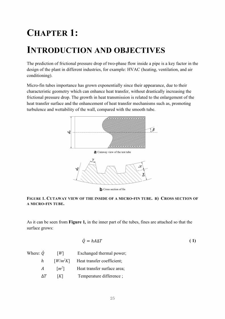
Micro-fin tubes importance has grown exponentially since their appearance, due to their characteristic geometry which can enhance heat transfer, without drastically increasing the frictional pressure drop. The growth in heat transmission is related to the enlargement of the heat transfer surface and the enhancement of heat transfer mechanisms such as, promoting turbulence and wettability of the wall, compared with the smooth tube.

FIGURE 1. CUTAWAY VIEW OF THE INSIDE OF A MICRO-FIN TUBE. B) CROSS SECTION OF A MICRO-FIN TUBE.

As it can be seen from Figure 1, in the inner part of the tubes, fines are attached so that the surface grows:

Where: �̇� [W] Exchanged thermal power;

ℎ [W/m2K] Heat transfer coefficient;

𝐴 [m2] Heat transfer surface area;

Δ𝑇 [K] Temperature difference ;

�̇� = ℎ𝐴Δ𝑇 ( 1)

26

On the one hand, Equation (1) points out that if h grows (due to the enhancement of heat transfer mechanisms), then �̇� increases, this growth is compared to the smooth tube through the enhancement factor:

𝐸 =ℎT9ℎU

( 2)

Where: 𝐸 [-] Enhancement factor; ℎT9 [W/m2K] Micro-fin tube heat transfer coefficient; ℎU [W/m2K] Smooth tube heat transfer coefficient;

On the other hand, it has to be reminded that, as it was said before, the frictional pressure drop also increases and this effect is captured by the penalization factor:

𝑃𝐹 =(𝑑𝑝𝑑𝑧)9,T9

(𝑑𝑝𝑑𝑧)9,U

( 3)

Where: 𝑃𝐹 [-] Penalization factor; (]^]_)9,T9 [Pa/m] Frictional pressure drop for the micro-fin tube;

(]^]_)9,U [Pa/m] Frictional pressure drop for the smooth tube;

These two factors have to be compared to see which tube matches better the particular characteristics of the plant, to obtain the highest increase of efficiency.

The advantages that micro-fin tubes present put them in the spot light of numerous studies. Most of them are related to condensation and evaporation, because they are the main processes taking place in the HVAC industry and because, as it will be corroborated in this work, micro-fin tubes have higher performances in two-phase flows.

These type of studies related to condensation and evaporation involve complex systems that give way to high uncertainty because the apparatus require high number of instruments characterized by non-zero uncertainty.

It is for this reason that, in this work, the frictional pressure drop of air-water flow in a micro-fin tube under adiabatic conditions will be studied, and it will be compared to these same flow inside a smooth-tube with the same inner diameter.

By choosing these particular conditions instead of the complex conditions for condensation or evaporation the uncertainties related to the system will be reduced and also the experiment complexity will be drastically diminished. The operating condition of adiabatic air-water flow

27

has been proved from the literature to be suitable also for the case of diabatic steam-water flow as far as, the determination of the pressure gradient is involved.

So in the end, the aim of this thesis is to find the correlations that best match the experimental data collected with the particular conditions used in this work. Also the penalization factor will be studied, trying to find any relevant information related to this ratio.

28

29

CHAPTER 2:

THEORETICAL BACKGROUND

2.1. FUNDAMENTAL QUANTITIES FOR TWO-PHASE FLOWS For a better comprehension of pressure drop evaluation some fundamental quantities have to be presented:

• Mass flux:

𝐺 [kg/(m2 s)] ;

• Gas mass flow rate:

Γb [kg/s] ;

• Liquid mass flow rate:

Γc [kg/s] ;

• Total mass flow rate of the two-phase flow:

Γ = Γb + Γc[kg/s] ;

• Average mass quality:

�̅� = fgf

[-] ;

• Gas volume flow rate:

𝑄b [m3/s] ;

• Liquid volume flow rate:

𝑄c [m3/s] ;

• Total volume flow rate of the two-phase flow:

𝑄 = 𝑄b + 𝑄c [m3/s] ;

• Average volume quality:

𝑥hiii =jgj

[-]

NOTE : In general 𝑥hiii ≠ �̅�, in fact :

𝑥hiii =1

1 +𝜌b𝜌c1 − �̅��̅�

( 4)

30

FIGURE 2. A) CROSS-SECTION OF A TWO-PHASE FLOW INSIDE A TUBE. B) DIFFERENTIAL CROSS-SECTION AREA 𝐝𝛀OF THE TUBE.

• Void fraction:

𝛼 = ]pg]p

[-] ;

Where: 𝑑Ωb [m3] Gas differential cross-section area; 𝑑Ω [m3] Total differential cross-section area;

• Average void fraction:

𝛼i = pgp

[-] ; Where: Ωb [m3] Gas cross-section area; Ω [m3] Total cross-section area;

• Superficial velocity for: - Gas:

𝑗b =]jg]p

[m/s] ;

- Liquid: 𝑗c =

]js]p

[m/s] ;

• Local velocity for:

- Gas:

𝑢b =]jg]pg

= ]jgu]p

= vgu

[m/s] ;

- Liquid: 𝑢c =

]js]ps

= ]js(%1u)]p

= vs(%1u)

[m/s] ;

• Cross-section average superficial velocity for:

- Gas: 𝚥b̅ =

jgp

[m/s] ; - Liquid:

𝚥c̅ =jsp

[m/s] ;

31

• Mixture velocity:

𝚥̅ = 𝚥b̅ + 𝚥c̅ =jgxjsp

= jp

[m/s] ;

• Cross-section average velocity for: - Gas:

𝑢biii =jguyp

= z̅guy

[m/s] ;

- Liquid: 𝑢cy = js

(%1uy)p= z̅s

(%1uy) [m/s] ;

• Slip ratio:

𝑠 = |g|s

[-] ;

• Average slip ratio:

�̅� = |giiii

|siii [-] ;

• Actual mass flux for:

- Gas: 𝐺b = 𝜌b𝑢ib [kg/m2/s] ;

- Gas: 𝐺c = 𝜌c𝑢ic [kg/m2/s] ;

• Apparent mass flux for: - Gas:

𝐺∗b = 𝜌b𝚥b̅ [kg/m2/s] ; - Liquid:

𝐺∗c = 𝜌c𝚥c̅ [kg/m2/s] ;

NOTE: The superficial velocity refers to the gas ( 𝚥b̅) or the liquid ( 𝚥c̅) flowing ALONE in the tube with their actual volume flow rate.

NOTE: As the apparent mass flux is related to the SUPERFICIAL velocity, it takes into account the phase flowing ALONE in the tube with its actual flow rate.

NOTE: In general 𝛼i ≠ �̅�, in fact :

𝛼i =1

1 + �̅�𝜌b𝜌c1 − �̅��̅�

( 5)

32

• Density of a two-phase mixture:

- Photographic density: 𝜌∗ = 𝛼i𝜌b + (1 − 𝛼i)𝜌c [kg/m3] ;

- Bulk density: 𝜌~ =

%2y�gx(��2y)�s

[kg/m3] ;

2.2. GOVERNING EQUATIONS OF TWO-PHASE FLOW

A study of governing equations has to be done before starting the experimental work on frictional pressure drop measurements, so that the data gathered can be perfectly understood.

First of all, pressure variation inside a pipe occurs due to many factors:

1. Friction: of the fluid with the pipe and of the phases between them.

2. Velocity variations along the pipe: because of variations in density or cross-section.

3. Velocity variations with time.

4. Gravity.

5. Exchange of heat and/or work.

To obtain the pressure drop all these factors have to be taken into account, and it can be achieved through balance equations, but some simplifying assumptions can be introduced to be able to solve these equations:

1. Steady-state conditions: No variation in time, this implies that velocity variations with

time won’t have to be taken into account.

2. One-dimension flow.

3. Constant properties.

4. Uniform cross-section: the term related to velocity variations due to cross-section

changes will not influence the pressure drop.

5. No flow work.

Applying all these simplifying assumptions we can take a differential (dz) of the tube, an example is shown in Figure 3, and study the balance equations that had been mentioned before:

33

FIGURE 3. FORCES APPLIED ON A TUBE DIFFERENTIAL.

The indexes related to the quantities have the following meanings: - g = gas - l = liquid - 1 = position z - 2 = position z+dz

• Mass balance:

𝑚𝑎𝑠𝑠𝑒𝑛𝑡𝑒𝑟𝑖𝑛𝑔 − 𝑚𝑎𝑠𝑠𝑒𝑥𝑖𝑡𝑖𝑛𝑔 = 0

Γb,% + Γc,% − (Γb,� + Γc,�) = 0

𝑑Γb𝑑𝑧 +

𝑑Γc𝑑𝑧 =

𝑑𝑑𝑧�Γb + Γc� =

𝑑Γ𝑑𝑧 = 0

For Γ = Ω𝐺; with Ω = 𝑐𝑡𝑒 :

Ω𝑑𝐺𝑑𝑧 = 0 →

𝑑𝐺𝑑𝑧 = 0 → 𝐺 = 𝑐𝑡𝑒

( 6)

• Momentum balance:

𝑓𝑙𝑜𝑤𝑜𝑓𝑚𝑜𝑚𝑒𝑛𝑡𝑢𝑚𝑒𝑥𝑖𝑡𝑖𝑛𝑔 − 𝑓𝑙𝑜𝑤𝑜𝑓𝑚𝑜𝑚𝑒𝑛𝑡𝑢𝑚𝑒𝑛𝑡𝑒𝑟𝑖𝑛𝑔 =

𝑟𝑒𝑠𝑢𝑙𝑡𝑎𝑛𝑡𝑜𝑓𝑓𝑜𝑟𝑐𝑒𝑠𝑎𝑝𝑝𝑙𝑖𝑒𝑑𝑡𝑜𝑐𝑜𝑛𝑡𝑟𝑜𝑙𝑣𝑜𝑙𝑢𝑚𝑒

Γb,�𝑢ib,� + Γc,�𝑢ic,� − �Γb,%𝑢ib,% + Γc,%𝑢ic,%�

=

𝑝%Ω − 𝑝�Ω − τsdz − 𝜌b𝑔𝑠𝑖𝑛𝜃Ωb𝑑𝑧 − 𝜌c𝑔𝑠𝑖𝑛𝜃Ωc𝑑𝑧

34

−]^]_= %

p]]_�Γb𝑢ib + Γc𝑢ic� + 𝜏

Up+ �𝛼i𝜌b + (1 − 𝛼i)𝜌c�

The term ( * ) can be rewritten as:

(∗) = 𝐺�𝑑𝑑𝑧 �

�̅��

𝛼i1𝜌b+(1 − �̅��)(1 − 𝛼i)

1𝜌c� = 𝐺�

𝑑𝑑𝑧 �

1𝜌Tiiii�

Where it is defined the momentum weighted specific volume:

𝑣Tiiii = �1𝜌Tiiii� = �

�̅��

𝛼i1𝜌b+(1 − �̅��)(1 − 𝛼i)

1𝜌c�

And making use of the definition of photographic density (𝜌∗), the next equation is obtained for the evaluation of the pressure drop:

−𝑑𝑝𝑑𝑧 = 𝐺�

𝑑𝑑𝑧 �

1𝜌T� + 𝜏

𝑠Ω + 𝜌

∗𝑔𝑠𝑖𝑛𝜃

( 7)

Where:

• (a): Accelerative term. • (f): Frictional term. • (g): Gravitational term. • s: Perimeter of the cross-section • 𝜏: sheer stress

We can observe from equation 7 that for the accelerative and gravitational term a model for the void fraction is needed. While for the frictional term a model for the sheer stress has to be applied.

• Energy balance:

𝑒𝑛𝑒𝑟𝑔𝑦𝑜𝑢𝑡𝑓𝑙𝑜𝑤 − 𝑒𝑛𝑒𝑟𝑔𝑦𝑖𝑛𝑓𝑙𝑜𝑤 = 𝑤𝑜𝑟𝑘𝑓𝑙𝑜𝑤 + ℎ𝑒𝑎𝑡𝑓𝑙𝑜𝑤

( * )

(a) (f) (g)

35

And developing the equation above, it is finally obtained:

−𝑑𝑝𝑑𝑧 =

12 �̅�~𝐺

� 𝑑𝑑𝑧 �𝑣b

� �̅�E

𝛼i� + 𝑣c� (1 − �̅�)

E

(1 − 𝛼i)�  + �̅�~𝑑𝑅i~𝑑𝑧 + �̅�~𝑔𝑠𝑒𝑛𝜃

( 8)

Where: ]Ki¡]_

[J/kg/m]: energy transformed into heat due to friction.

In these case ]Ki¡]_

and 𝛼i will have to be estimated.

From the equations obtained by applying momentum and energy balance, it can be observed that the terms referring to accelerative frictional and gravitational pressure drop do not need to coincide, but the sum of the three has to be equal.

2.3. PRESSURE GRADIENT EVALUATION

As it was seen in the previous section some models have to be applied to evaluate some quantities that appear in the pressure drop equation (𝛼i and 𝜏).

In this thesis, only the frictional pressure drop will be studied as the tube is horizontal (so there is no gravitational pressure drop) and the quality is maintained constant in all the tube (so the accelerative term does not contribute to the pressure gradient).

The classic models that are normally used for two-phase flows are the next three ones:

2.3.1. HOMOGENEOUS FLOW MODEL

This model considers the two phase flow as a single phase flow. The properties are assumed to be the mean between the actual phases (in this particular case: air and water).

In the homogeneous flow model it is stablished that gas and liquid have equal velocities (𝑢ib = 𝑢ic), these assumption implies:

�̅� = 1 → 𝛼i = �̅�h → �̅�~ = 𝜌∗

( 9)

(a) (f) (g)

36

So that the equation for pressure drop will be the same for momentum and energy balance:

−]^]_= 𝐺� ]

]_(�̅�~) + 𝜏

Up+ �̅�~𝑔𝑠𝑖𝑛𝜃

( 10)

Accelerative and gravitational terms could be easily obtained, but in this thesis they will be always zero, as it was already explained and only the frictional component will be computed. The frictional pressure drop for the two-phase flow can be rewritten as:

Where: 𝑓¢^ [-] Two-phase friction factor.

This new expression of the pressure drop is obtained through dimensionless study of the sheer stress. The friction factor for the two-phase flow can adopt different expression depending on the model applied and the correlation used [1]. For the homogeneous flow model, the two-phase friction factor is evaluated from single-phase friction factor relationships replacing a suitable defined mean viscosity (�̅�) that will be calculated in different ways depending on the correlation chosen.

Where: A, m [-] constants depending on the model;

𝑅𝑒¢^ =fD¤y

[-] Two-phase Reynolds number;

This model approaches a two-phase flow by a single-phase one, with the same thermodynamical properties. These assumptions can be considered valid if the phases are sufficiently mixed (one of the phases is finely dispersed in the other) and the Reynolds number is sufficiently high (so that velocities are high enough). In this thesis the correlations based on homogeneous flow model are: McAdams et al. (1942) [2], Shannak (2008) [3], Chent et al. (2001) [4].

2.3.2. SEPARATED FLOW MODEL

As the name of the model suggests, this model supposes the two phases flowing separated. This means that the two-phase flow is taken as two single-phase flows. The model is based on the use of the two-phase frictional multiplier 𝜙(�, where the subscript i can be l, g, lo, go with meaning of liquid, gas, liquid-only, gas-only, respectively. In this way the model can be branched in two parts:

B]^¦]_G¢^= 𝜏 U

p=

�9§-f§-¨

©§-D

( 11)

𝑓¢^ = 𝐴𝑅𝑒¢^1T

( 12)

37

FIGURE 4. REPRESENTATION OF THE SEPARATED FLOW MODEL

• Liquid (𝜙c�) and gas (𝜙b�) based two-phase friction multipliers methods. The

frictional multiplier is defined as the ratio of the two-phase frictional pressure gradient over the pressure gradient that would arise if the i-th phase flowed alone in the pipe:

Where the frictional pressure drop for the single-phase is evaluated according to:

The friction factor can be computed with any of the correlations developed for single-phase flow such as: Pethukov or Blasius correlations.

The first one to develop these frictional pressure multiplier were Lockhart and Martinelli (1949) [5], that came up with a parameter that is named after them, the Lockhart-Martinelli parameter X.

This parameter relates liquid pressure drop over gas pressure drop, and the frictional pressure multipliers (𝜙c�𝑎𝑛𝑑𝜙b�) are found to be function of this ratio:

The only inconvenient found in their model was that it was a graphical method and so, it was not very practical.

𝜙c� = B]^¦]_G¢^

B]^¦]_Gc

ª

( 13)

𝜙b� = B]^¦]_G¢^

B]^¦]_Gb

«

( 14)

B]^¦]_G(= �9+f+

¨

©+D where the subscript i is l or g.

( 15)

𝑋� =�0-¦0­ �s

�0-¦0­ �g

( 16)

38

It was then when Chisholm (1967) [6] proposed an empirical correlation between the Lockhart-Martinelli parameter, the two-phase frictional multipliers and a parameter C that is dependent on the flow regime. The relation was no longer graphical and was much more practical.

These model gave way to many other researchers studies and correlations. In this thesis the next correlations will be used: Chisholm (1967), Sun and Mishima (2009) [7], Wang et al. (1997) [8], Murata (1993) [9], Haraguchi (1994) [10], Kedzierski (2004) [11] .

• Liquid-only (𝜙c®� ) and gas-only (𝜙b®� ) based two-phase friction multipliers methods. The frictional multipliers is defined as the ratio of the two-phase frictional pressure gradient over the pressure gradient that would arise if the phase flowed alone in the pipe with the total mass flux of the two-phase flow:

Where the frictional pressure drop for the single-phase is evaluated according to:

The friction factor can be computed with any of the correlations developed for single-phase flow such as: Pethukov or Blasius correlations. In this thesis the next correlations will be used following these model: Muller-Steinhagen and Heck (1986) [12], Tran et al (1999) [13], Cavallini et al (1999) [14].

The separated flow model is completely different from the homogeneous one, in which the phases had to be very mixed. This model will be more suitable for situations in which the phases are more apart.

𝜙c� = 1 + ¯°+ %

°¨

( 17)

𝜙c®� = B]^¦]_G¢^

B]^¦]_Gc®

ª

( 18)

𝜙b®� = B]^¦]_G¢^

B]^¦]_Gb®

«

( 19)

B]^¦]_G(®=

�9+±f§-¨

©+D where i is l or g.

( 20)

39

2.3.3. FLOW PATTERN DEPENDANT MODEL

And last, but not least, the flow pattern dependant models that take into account the type of flow that takes place in the tube (annular, wavy, mist, slug…) and find correlations suitable ONLY for that type of flow.

In this thesis none of the correlations used follow these kind of model, they only follow the two preceding ones.

FIGURE 5. FLOW PATTERNS OF TWO-PHASE FLOWS [15]

2.4. CORRELATIONS

The total pressure drop in a tube is composed by three terms, as it has been said before, and just the frictional pressure drop will remain in these study due to:

• Accelerative pressure drop: There is no variation of quality along the tube, so there

is no accelerative component.

• Gravitational pressure drop: The tube is in a horizontal position so that gravitational forces don’t appear.

• Frictional pressure drop: It is the only component that will last.

40

So the equation for pressure drop in this experimental system will be reduced to:

The frictional pressure drop can be computed through experimental correlations. The correlations used in the thesis are multiple and follow the different models presented in the section above.

It will be observed that for some of the correlations great deviations are found, these is not a surprise as the correlations used might have been obtained for particular systems that do not match perfectly the system of the thesis.

The correlations will be presented grouped by single-phase flow correlations and tow-phase flow correlations.

2.4.1. SINGLE-PHASE FLOW CORRELATIONS:

For single-phase flow pressure drop computation, the Darcy friction factor formulae are needed. They are equations that make possible the computation of the Darcy friction factor (also known as, simply, friction factor), to then calculate the pressure drop inside a pipe.

For the laminar flow, the friction factor is computed as:

While for the turbulent flow, the correlations used for the single phase flow of water are the three next ones [2]:

• Blasius correlation: It is the easiest formula that can be used to compute the friction factor in smooth pipes (as it does not take into account any roughness):

• Petukhov correlation: It is also developed for smooth pipes and the computation is done using the next formula:

�𝑑𝑝9𝑑𝑧  

= �

𝑑𝑝9𝑑𝑧  

²+ �

𝑑𝑝9𝑑𝑧  

b+ �

𝑑𝑝9𝑑𝑧  

9= �

𝑑𝑝9𝑑𝑧  

9

( 21)

𝑓 = I³KL

; ( 22)

𝑓 = 0.316𝑅𝑒1¶.�· ; ( 23)

𝑓 = (0.79 ln(𝑅𝑒) − 1.64)1�; ( 24)

41

• Haaland correlation: Colebrook’s equation expresses the friction factor as a function of the Reynolds number and the relative roughness (as the correlation is developed for smooth and rough tubes). The problem with this equation is that an iterative process is needed to find the Darcy friction factor. Instead, approximations of the Colebrook equation allow calculating the friction factor without the need of iteration. One of the approximations is the Haaland approximation:

2.4.2. TWO-PHASE FLOW CORRELATIONS:

2.4.2.1. Homogeneous flow model correlations:

In homogeneous correlations the key point is the estimation of the two-phase flow Reynolds number to match the single-phase flow friction factor correlations. As it was introduced in section (2.3.1) the frictional pressure drop in this model is obtained as:

Where:

- The two-phase flow density is computed as:

- 𝑓¢^ based on Petukhov correlation (Equation 24), but instead of Re for a single-phase flow, a Retp, for the two-phase flow, will have to be computed.

• McAdams correlation (1942) [2]:

McAdams proposed the computation of the two-phase flow Reynolds number as a single-phase flow Reynolds number with a two-phase flow viscosity, that follows, by analogy, the expression of the two-phase flow density:

%89= −1.8𝑙𝑜𝑔 ABC D⁄

E.FG%.%%

+ I.JKLM; ( 25)

�𝑑𝑝9𝑑𝑧  

¢^=2𝑓¢^𝐺¢^�

𝜌¢^𝐷

( 26)

%©§-

= ½©g+ %1½

©s ( 27)

42

• Chen et al. (2001) [4]: Proposes a modification on the homogeneous flow model correlation using W. W is a parameter obtained from the measured data of air-water and R410A.

Where:

- B]^¦]_G¢^,¾®T

is obtained from McAdams model.

- W parameter depends on Bond number:

Ω ¿1.2 − 0.9 exp(−𝐵𝑜) 𝐵𝑜 < 2.5;

1 +𝑊𝑒¶.�

exp(𝐵𝑜¶.E) − 0.9 exp(−𝐵𝑜) 𝐵𝑜 ≥ 2.5;

Where: 𝐵𝑜 = 𝑔 (©s1©g)(D �⁄ )¨

É and 𝑊𝑒 =

f§-¨ D

É©§- ;

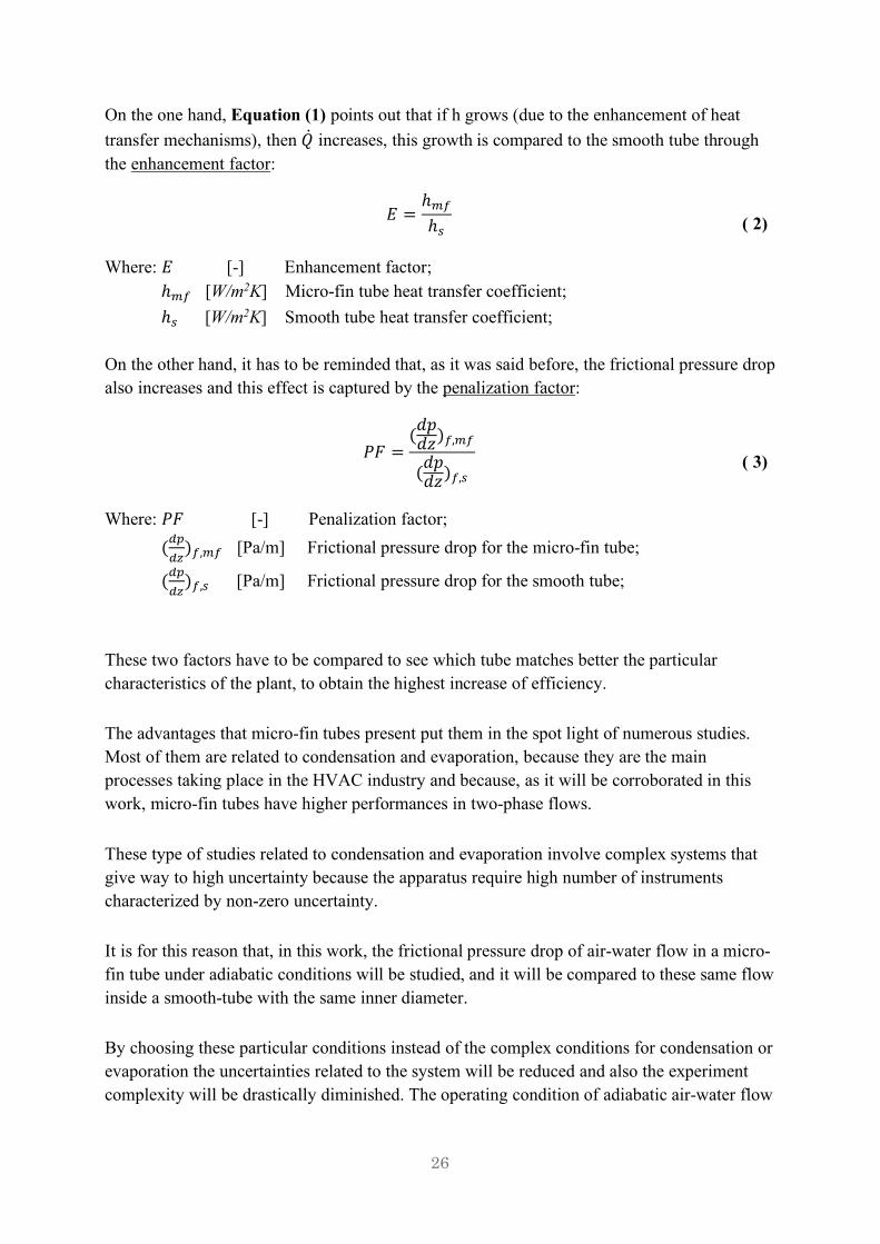
• Shannak (2008) [3]: A new prediction model for pressure drop of two-phase flow in pipes is proposed by Shannak. The model includes a new definition of the friction factor and Reynolds number the for two-phase flow, given as the ratio of the sum of inertial force of each phase and that of the sum of viscous force of each phase.

The correlation is obtained from experimental data gathered from the flow of air water two-phase flow in a vertical and horizontal smooth and relatively rough pipes.

The new Reynolds number for two-phase flow is defined as:

And the new two-phase friction factor:

- 𝑅𝑒¢^ =fD¤§-

;

( 28)

- %¤§-

= ½¤g+ %1½

¤s ;

( 29)

�𝑑𝑝9𝑑𝑧  

¢^= Ω�

𝑑𝑝9𝑑𝑧  

¢^,¾®T

( 30)

𝑅𝑒¢^ =½¨x(%1½)¨�©g ©s⁄ �

�½¨ KLgª �x((%1½)¨ KLs⁄ )�©g ©s⁄ �

( 31)

%89§-

= −2𝑙𝑜𝑔 A %E.F¶I·

C]− ·.¶³·�

KL§-𝑙𝑜𝑔 � %

�.Ê�·FBC]G%.%¶JÊ

+ ·.Ê·¶IKL§-Ë.ÌÍÌ�

�M

( 32)

43

FIGURE 6. REPRESENTATION OF FRICTION FACTOR TO REYNOLD NUMBER FOR DIFFERENT RELATIVE ROUGHNESS [3]

2.4.2.2. Two-phase flow model correlations.

As it was introduced in the theoretical background, the two-phase flow models can adopt two different formulation, liquid and gas frictional multipliers or liquid only gas only frictional multipliers. The correlations will be presented following these two branches.

i. Liquid and gas frictional multipliers.

• Chisholm correlation [6]:

Chisholm transformed Lockhart-Martinelli graphical procedure, into a numerical one by developing the correlation:

Where:

o C [-] Constant that varies with flow regime following Table 1. It is to be remembered that, to know if a gas or liquid is in turbulent o laminar flow the following inequality is used:

- Laminar: 𝑅𝑒( < 2300𝑤𝑖𝑡ℎ𝑖 = 𝑔, 𝑙 ; - Turbulent: 𝑅𝑒( > 2300𝑤𝑖𝑡ℎ𝑖 = 𝑔, 𝑙 ;

Where: 𝑅𝑒( =fD¤+[−]𝑤ℎ𝑒𝑟𝑒𝑖 = 𝑔, 𝑙 Reynolds number for the

liquid (l) and for the gas (g).

𝜙c� = 1 +𝐶𝑋¢¢

+1𝑋¢¢�

( 33)

44

TABLE 1. CONSTANT VARIATION WITH FLOW REGIME.

o 𝑋¢¢� =�0-¦0­ �s

�0-¦0­ �g

= �¤s¤g�¶.%B©g©sG¶.·B%1½̅

½̅G¶.J

[-] Lockhart-Martinelli

parameter for turbulent-turbulent flow.

Once 𝑋¢¢ is found and C is determined through flow regime, 𝜙c� can be computed and with the initial equation:

The frictional pressure drop can be obtained by calculating the pressure drop in the smooth tube of a single-phase flow of liquid:

In this thesis, the friction factor for single-phase flow will be implemented using Pethukov’s correlation (Equation 24). As it will be seen, further in the thesis, Pethukov’s correlation follows the experimental data with MARD% of 4.192, so it is a good correlation for the particular case treated in the work.

• Sun and Mishima correlation (2008) [7]:

A modified Chisholm correlation is proposed, giving a better result than all the correlations evaluated for the data gathered from 18 published papers, of which the working fluids are: different refrigerants (R123, R134a, R22…), CO2, water and air.

The hydraulic diameter ranges from 0.506 to 12mm; Rel from 10 to 37000, and Reg from 3 to 400000. So laminar an turbulent flow are studied in these report.

The correlation proposed is based on the concept that C is not constant, but a parameter that is affected by flow conditions:

- If the flow is laminar (Rel < 2000 or Reg < 2000):

C GAS LIQUID 20 Turbulent Turbulent 12 Turbulent Laminar 10 Laminar Turbulent 5 Laminar Laminar

B]^¦]_G= B]^¦

]_Gc𝜙c�

( 34)

B]^¦]_Gc= �9sfs

¨

©sD ;

( 35)

𝐶 = 26 B1 + KLs%¶¶¶

G Ò1 − 𝑒𝑥𝑝 B 1¶.%·E¶.�FÓ²x¶.Ê

GÔ ; ( 36)

45

- If the flow is turbulent (Rel > 2000 and Reg > 2000):

Where:𝑅𝑒c [-] Reynolds number of the liquid phase;

𝑅𝑒b[-] Reynolds number of the gas phase; 𝐿𝑎 [-] Laplace number;

Once the constant C has been determined, the value of 𝜙c� can be obtained:

Where: n = 1 for laminar condition ( Rel < 2300 );

n = 1.19 for turbulent condition ( Rel > 2300 );

• Wang et. al. correlation (1997) [8]: In this study two-phase flow friction characteristics for R22, R134a and R407c inside a 6.5 mm smooth tube are reported. The range of mass flux is between 50 and 700 kg/m2/s.

Tests were conducted adiabatically. In this report, a dependence of the multipliers with the mass flux was observed, and so the implementation of the pressure drop is divided with dependence on the mass flux:

- For G = 50-100 kg/m2/s:

- For G > 200kg/m2/s:

For the values of G Î (100, 200) kg/m2/s, an average two-phase multiplier was implemented.

𝐶 = 1.79�𝑅𝑒b𝑅𝑒c

�¶.³

�1 − 𝑥𝑥 �

¶.·

( 37)

𝜙c� = 1 + ¯°Ö+ %

° ;

( 38)

𝐶 = 4.566 × 101I𝑋¶.%�Ê𝑅𝑒c®¶.JEÊ �©s©g�1�.%·

�¤s¤g�·.%

; ( 39)

𝜙b� = 1 + 𝐶𝑋 + 𝑋� ; ( 40)

𝜙b� = 1 + 9.397𝑋¶.I� + 0.564𝑋�.³· ; ( 41)

46

• Murata correlation (1993) [9]: Forced convective boiling of nonazeotropic mixtures inside horizontal tubes was investigated in this report. R123 and a mixture of R123 and R134a were measured in both a smooth tube and a spirally grooved tube. A correlation was proposed for smooth tubes and grooved tubes:

- For smooth tubes:

- For the grooved tube:

Also the pressure drop for the liquid flow is defined as:

• Haraguchi correlation [10]: Condensation experiments on horizontal smooth and micro-fin tubes have been performed with two-phase refrigerant flow. Mass flux varies from 90 to 400 kg/m2/s, and heat is also provided in the range of 3 to 33 kW/m2. The developed correlation is related to the gas frictional multiplier:

Where the geometrical parameters of the micro-fin tube are accounted by the equivalent diameter (De) present in the correlation. This diameter is implemented using Ac that is the cross sectional area taking into account the variations due to the fins. The subscript e, refers to equivalent.

𝜙c = 1 + 2.1(1 𝑋¢¢)⁄ ¶.J ;

( 42)

𝜙c = 1 + 2.5(1 𝑋¢¢)⁄ ¶.J ;

( 43)

−B]^¦]_Gc= ¶.%ʳ

KLsË.¨

{f(%1½)}¨

�𝐷(𝜌c where: 𝑅𝑒c =

f(%1½)D+¤s

;

( 44)

𝜙b = 1.1 + 1.3 Ú °§§f

ÛbD/©g(©s1©g)ÜË.ÝÞ

¶.E· ;

( 45)

𝑓L,b = 0.046𝑅𝑒L.b1¶.� ;

( 46)

𝐷L = ß³àáâ

;

( 47)

𝑅𝑒L,b =fD/½¤g

; ( 48)

47

• Kedzierski correlation (2004) [11]:

This paper presents a study of pressure drops during condensation inside a smooth tube, a helical micro-fin tube and a herringbone micro-fin tube. Experiment was carried with refrigerants (R22, R407C and R134a) flowing through the tube of a concentric heat exchanger at a saturation temperature of 40ºC. Mass fluxes ranged from 400 to 800 kg/m2/s. The correlation proposed by this report is a modification of a helical micro-fin correlation to suit a herringbone micro-fin tube.

Where: B ààÖG = 1 − ³¾ã¢

âD+¨ä®Uå

A is the actual cross-sectional flow are of the tube and An the nominal flow area based on the fin-root diameter, h represents the fin height, n the number of fins, t the fin thickness and b the helix angle of the fins.

ii. Liquid and gas only Frictional multipliers

• Muller-Steinhagen and Heck correlation (1986) [12] : The papers proposes a new correlation for two-phase flow in smooth pipes:

Where: 𝑌� = B]^¦]_Gc®

B]^¦]_Gb®

« ;

x [-] air mass quality;

To calculate the pressure drop for liquid and gas only, it is to be remembered an equation already presented:

𝜙c� = 1.376 + F.�³�°§§�.çÝÝ

; ( 49)

B]^¦]_G= B]^¦

]_Gc®𝜙c� ; ( 50)

B]^¦]_Gc®= �9s±f¨(%1½)¨

©sD+ ; ( 51)

𝑓c® = 0.046𝑅𝑒c1¶.� BD+D/G B à

àÖG¶.·(𝑠𝑒𝑐𝛽)¶.F·

( 52)

𝜙c®� = 𝑌�𝑥E + (1 − 𝑥)%/E[1 + 2𝑥(𝑌� − 1)]

( 53)

48

Where the subscript i is to be substituted by l or g.

• Tran et. al. correlation (2000) [13]:

Three refrigerants (R134a,R12 and R113) were tested at different pressures in two sizes of round tubes and one rectangular channel. With the data collected a new correlation for two-phase pressure drop during boiling was obtained for small channels:

Where: La [-] LaPlace number ;

x [-] air mass quality ;

• Cavallini correlation (1999 [14]):

Condensation phenomena is studied, and pressure drop is collected for refrigerants inside commercially available tubes with enhanced surfaces of different types.

A new correlation is proposed for adiabatic flow:

B]^¦]_G(®=

�9+±f§-¨

©+D ( 54)

𝜙c®� = 1 + (4.3𝑌� − 1){[𝑥(1 − 𝑥)]¶.ÊF·𝐿𝑎 + 𝑥%.F·}

( 55)

𝜙c®� = 𝐸 + (3.23𝐹𝐻) 𝐹𝑟¶.¶³·𝑊𝑒¶.¶E·⁄ ; ( 56)

𝐸 = (1 − 𝑥)� + 𝑥� (𝜌c𝑓b®) (𝜌b𝑓c®)⁄ ; ( 57)

𝐹 = 𝑥¶.FÊ(1 − 𝑥)0.224 ; ( 58)

𝐻 = �𝜌c 𝜌b⁄ �¶.J%�𝜇b 𝜇c⁄ �¶.%J(1 − 𝜇b 𝜇c⁄ )¶.F ; ( 59)

𝐹𝑟 = 𝐺� (𝑔𝐷𝜌T)⁄ ; ( 60)

𝑊𝑒 = 𝐺�𝑑 (𝜌T𝜎)⁄ ; ( 61)

𝜌T = 𝜌c𝜌b/Û𝑥𝜌c + (1 − 𝑥)𝜌bÜ ; ( 62)

49

TABLE 2. FORMULATION OF FRICTION FACTOR FOR CAVALLINI CORRELATION.

Where the relative roughness is defines as:

Finally once 𝜙c®� is computed the pressure drop can be obtained by the usual

equation:

Flow 𝒇𝒍𝒐 = 𝒎𝒂𝒙(𝒇𝒍𝒐𝟏, 𝒇𝒍𝒐𝟐) 𝒇𝒈𝒐 = 𝒎𝒂𝒙(𝒇𝒈𝒐𝟏, 𝒇𝒍𝒈𝟐)

Turb 𝑓c®% = 0.079(𝑅𝑒c®)1¶.�· 𝑓b®% = 0.079(𝑅𝑒b®)1¶.�·

Lam 𝑓c®% = 16/𝑅𝑒c® 𝑓b®% = 16/𝑅𝑒b®

(4𝑓c®�)1¶.· = 1.74 − 2𝑙𝑜𝑔%¶ �2𝑒𝐷 � (4𝑓b®�)1¶.· = 1.74 − 2𝑙𝑜𝑔%¶ �

2𝑒𝐷 �

LD= 0.18 B¾

DG (0.1 + 𝑐𝑜𝑠𝛽)ª ;

( 63)

𝜙c®� = �𝑑𝑝9𝑑𝑧  

¢^�𝑑𝑝9𝑑𝑧  

c®«

( 64)

50

51

CHAPTER 3:

EXPERIMENTAL SET UP.

3.1. INSTRUMENTATION DESCRIPTION:

The system is composed of different instrumentations that allow the realization of the experimental analysis. As the experiment is based on a two phase flow, the test section will have to be provided of both: water and air.

First of all, the water circuit, which will also be in charge of providing the single-phase flow for the calibration of the system and the water-flow in the micro-fin tube. The water is pumped from the storage tank with a centrifugal pump that guides the water through the: thermometer, pressure gauge and volume flow rate measurement section, to the mixing section (with air) and finally to the test section, from which the water flows back to the tank where it is separated from air.

The volume flow rate of water can be adjusted thanks to the volume flow meters already mentioned, which are in fact three rotameters in parallel that work for different flow rates:

- Small volume flow meter: 𝑄 ∈ (10 − 100)[𝑙/ℎ] ; - Intermediate volume flow meter: : 𝑄 ∈ (40 − 400)[𝑙/ℎ] ; - Big volume flow meter:𝑄 ∈ (0.25 − 2.5)[𝑚𝑐/ℎ] ;

Secondly, the air circuit, that works similarly to the water circuit.

The compressed air is provided from the building auxiliary supply system and again goes through the thermometer, pressure gauge and volume flow meters. The air pressure is controlled with a pressure control valve to set the desired pressure of 4 bar before entering the air volume flow meters which, again, are three rotameters in parallel for different flow rates:

- Small volume flow meter: 𝑄 ∈ (10 − 190)[𝑛𝑙/ℎ] ; - Intermediate8 volume flow meter: : 𝑄 ∈ (100− 850)[𝑛𝑙/ℎ] ; - Big volume flow meter:𝑄 ∈ (400 − 4000)[𝑛𝑙/ℎ] ;

But in this case there is also a bypass in parallel with the three lines to prevent breaks in the rotameters due to sudden peaks of pressure in the starting-up of the system.

After the rotameters, the air is already adjusted and it is ready to enter the mixing section. Once it is mixed with water, the two-phase flow enters the test section. When coming out of the test section the air flow with the water into the tank, there the air is separated from water and vented into the environment .

52

The mixing section is common of the two circuits, it is composed of the two entries, water and air, and a transparent tube that gives time for the two fluids to mix and stabilize.

The test section is a copper tube which will be different for the different experiments.

First of all, a smooth tube will be used and the geometric characteristics of these tube are represented on Table 3.

Smooth tube L = 1.295 m d = 0.00892 m

TABLE 3. GEOMETRIC CHARACTERISTICS OF THE SMOOTH TUBE.

Secondly, for the micro-fin tube, geometric characteristics are presented in Table 4. It can be observed from the table that, the micro-fin tube has two type of fins with different heights as it is shown in Figure 7.

FIGURE 7. SCHEME OF THE TYPES OF FINS IN THE MICRO-FIN TUBE.

TABLE 4. GEOMETRIC CHARACTERISTICS OF THE MICRO-FIN TUBE

The final but most important part of the test section is the pressure transducer, that measures the pressure at the start of the test section and the end of that same one. This is achieved by two small plastic tubes filled with water that hydraulically conduct the pressure to the pressure transducer, one at the beginning and other at the end of the test section. As the pressure transducer measures only one pressure at a time the ducts are joint in a three way valve, so that only the upstream or downstream pressure is measured.

Micro-fin tube

Internal diameter (di) = 0.00892 m

External diameter (de) = 0.0095 m

L = 1.298 m

Cross section area (W) = 61.72 mm2

Wet perimeter = 39.9 mm2

Fin type 1 Fin type 2

Number (n) = 27 Number (n) =

Height (h) = 0.16 mm Height (h)= 0.23 mm

Fin angle (g) = 40º Fin angle (g) = 40º

Helix angle (b) = 18º Helix angle (b) = 18º

53

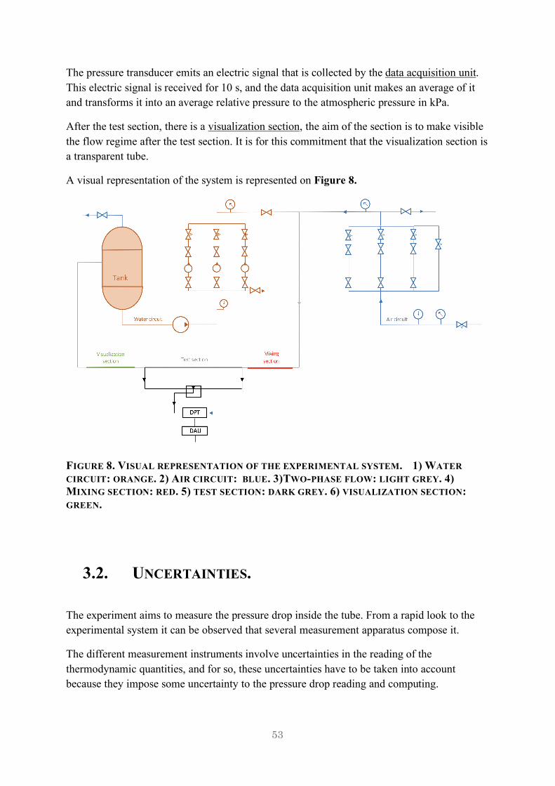
The pressure transducer emits an electric signal that is collected by the data acquisition unit. This electric signal is received for 10 s, and the data acquisition unit makes an average of it and transforms it into an average relative pressure to the atmospheric pressure in kPa.

After the test section, there is a visualization section, the aim of the section is to make visible the flow regime after the test section. It is for this commitment that the visualization section is a transparent tube.

A visual representation of the system is represented on Figure 8.

FIGURE 8. VISUAL REPRESENTATION OF THE EXPERIMENTAL SYSTEM. 1) WATER CIRCUIT: ORANGE. 2) AIR CIRCUIT: BLUE. 3)TWO-PHASE FLOW: LIGHT GREY. 4) MIXING SECTION: RED. 5) TEST SECTION: DARK GREY. 6) VISUALIZATION SECTION: GREEN.

3.2. UNCERTAINTIES.

The experiment aims to measure the pressure drop inside the tube. From a rapid look to the experimental system it can be observed that several measurement apparatus compose it.

The different measurement instruments involve uncertainties in the reading of the thermodynamic quantities, and for so, these uncertainties have to be taken into account because they impose some uncertainty to the pressure drop reading and computing.

54

The pressure difference is directly measured by the differential pressure transducer, for this, the uncertainty of the measurement is the uncertainty of the instrument itself.

In the data processing other quantities are needed to compute the experimental pressure drop and pressure drop from the different correlations.

The quantities taken from the system are:

- Water temperature. - Water volume flow rate. - Water pressure. - Air temperature. - Air volume flow rate. - Air pressure.

In Table 5 all the information related to the uncertainties of the measurement apparatus are present.

TABLE 5. INSTRUMENTATION UNCERTAINTIES.

3.3. EXPERIMENTAL SET-UP

The next topic to discuss is the experimental procedure that takes place.

3.3.1. OPERATING CONDITIONS First of all, the operating conditions for the experiment had to be selected and they are presented in Table 6:

- For the smooth tube: The range of operating conditions is selected with the Mandhane Map, in order to have annular flow practically through all the experiment. It was also taken into account the limiting condition of the differential pressure transducer, which has a maximum measurement of 70 kPa.

- For the micro-fin tube: The flow range of gas chosen to match the typical mass flux (G) for HVAC plants chillers and condensers, that characterised by an annular flow.

UNCERTAINTIES Three water flow-rates ±3% f.e.

Three air flow-rates ±3% f.e. Differential pressure transducer ±1.5% f.e.

55

Even though the aim was to obtain all the points related to this range, some points would not be obtained because, as it was said, the limit of the pressure transducer inhibits the acquisition of some high mass flux flows.

Single-phase Two-phase G [kg/(sm2)] G [kg/(sm2)] x [-]

Smooth 220-1800 220-1800 0.012-0.515 Micro-fin 50-480 50-480 0.012-0.515

TABLE 6. OPERATING CONDITIONS OF THE EXPERIMENT.

3.3.2. EXPERIMENTAL PROCEDURE: The thesis proceeds with 4 experiments:

i. Single-phase flow of water inside a smooth tube (Calibration experiment). ii. Two-phase flow air-water inside a smooth tube.

iii. Single-phase flow of water inside a micro-fin tube. iv. Two-phase flow air-water inside a micro-fin tube.

The experiments for single-phase follow one procedure, while for two-phase flow, another scheme is put in practice so, the explanation will be grouped as single-phase procedures and two-phase procedures.

3.3.2.1. Experimental procedure for single-phase flow: In this section the procedure for single-phase flow measurements will be explained. This procedure applies equally to the smooth tube and micro-fin tube.

The smooth tube single-phase flow will be used for the calibration of the system.

The system is started by opening the valves to let the water run inside the circuit and by turning on the water pump.

Once the system is started, the following steps have to be followed to collect the data:

1. The water flow has to be fixed to the desired value by making use of the different volume flow meters. In this case, as the range of water flow for single-phase flow goes from 50 to 400 l/h, the small and the intermediate flow meter will be used.

56

2. Once the flow of water is checked to be at the desired value, the next step is to measure the pressure difference. For this activity, the differential pressure transducer is the key instrument.

When steady-flow is reached, the data can be taken by telling the control unit to obtained the data measured by the pressure transducer.

It is important to remember that, the pressure transducer does NOT measure pressure difference, but the pressure at the inlet and outlet of the tube separately by making use of the three way valve. So, once a pressure is collected, the three way valve has to be shifted to the other end so that the other pressure is taken by the control unit.

3. After taking the two pressures for the specific volume flow rate, the next step is to re-start the process (by going back to 1) with a new volume flow rate, so that the pressure difference is obtained for all the volume flow rates from 50 to 400 l/h with steps of 25 l/h.

4. When the whole data for the range is obtained, the same procedure will be done 10 times to obtain 10 pressure difference data for each volume flow rate, an average of these data is made to reduce errors.

To reduce any type of induced errors due to human operation, the procedure will be changed by swapping the starting point from 50 to 400 l/h, so that one time the procedure is started from the bottom and going up, and the next time it is started from 400 and going down to 50 l/h.

In the end, as the procedure is repeated 10 times and the pressure difference is obtained for 15 volume flow rates in each sequence, the total data collected for the single-phase flow will be 150 (without taking into account any limitations by the pressure transducer’s maximum value).

When all the measurements needed for the data processing have been collected, the last thing to do is turning of the system. For that, the water pump will be turned off and the valves related to water flow meters will be closed, the air system will be started to dry the tube from any water that was attached to the wall to prevent the tube from fouling.

Once the mixing section, the test section and the visualization section are dried, the air circuit can be turned off and the single-phase flow experiment gets to its end.

3.3.2.2. Experimental procedure for two-phase flow: The experiment in this thesis will be run, first on the smooth tube and secondly on the micro-fin tube, but the procedure for both is the same.

57

First thing to do is to start up the system. The two-phase flow is set by opening: the water circuit first and then the air circuit.

Once an stable two-phase flow is achieved and taking care that the small tubes that connect the test section with the differential pressure transducer are filled completely with water (no bubbles of air, as they would perturb the measurements) the data collection can start:

1. The water flow is fixed at the level required (starting, for example, from the lowest range of Ql=10 l/h).

2. The air flow is to be adjusted (starting, for example, also from the bottom

Qg=500 l/h). In this step the regulation is very important.

As the air volume flow rate is changed, the pressure of the air (that is to be kept constant at 4 bars at the pressure measurement device at the exit of the volume flow meters) will change. This phenomena occurs because, at higher flow rates the pressure drop is also higher, and so for air entering the flow meters at a constant pressure, it is obvious, that the pressure at the exit will change.

The regulation can be achieved by varying the pressure entering the air circuit with the pressure valve, so that the pressure shown in the pressure measurement device is constant an equal to 3 bars (which is relative pressure compared to the atmospheric one, so the real pressure is 4 bars).

3. Once the air flow rate is fixed, the water flow rate has to be checked and

adjusted if any variations have appeared due to the fluctuations in the air flow rate.

4. After the first three steps, the two-phase flow wanted is obtained and the

next thing to do is measure. As it was said before, to measure the pressure, a differential pressure transducer is used. The information that the experiment looks to obtain is the pressure drop, and implies measuring pressure at the inlet and at the outlet, to obtain pressure difference that will then be transformed into pressure drop. The data are subtracted by changing the three way valve position, letting the data acquisition unit obtain the information from upstream and downstream the test section. Top and bottom pressures will be taken 5 times each, to obtain in this way a better measurement by doing the average. While all of the pressure data points are being taken, also temperature of air and water has to be collected.

58

5. The following step will be repeating points 2, 3 and 4 for all the air volume flow rate range, with jumps of 500 l/h. These would be: 500 l/h, 1000 l/h, 1500 l/h… and so on, until 4000 l/h is reached.

These means 7 different air flow rate data points obtained for each water flow rate.

6. Last but not least, once the data for all the air flow rates are collected, all

the steps have to be repeated (1-6) for the next water flow rate. Water flow rate range varies from 10-100 l/h, with steps of 10 l/h. These means: 10 l/h, 20 l/h, 30 l/h… and so on, until 100 l/h is reached.

This means that there are 10 different water flow rates points, for which there are 7 air flow rates, that makes a number of 70 data points for each experiment.

The last statement would be real if the differential pressure transducer did not have a limit pressure measurement of 70 kPa, that will imply some data at high water and air mass flow rate will not be able to be taken.

Once all the data have been collected the system has to be turned off by closing the water circuit and then the air circuit, leaving it open a few minutes to dry the system and prevent fouling.

3.3.3. SYSTEM CALIBRATION:

Before starting the actual experiment a calibration of the system needs to be done to see if the system works properly and to adjust the inner diameter of the tube which tolerance is unknown as it was not specified by the producer.

For the calibration, a single-phase flow of water is used with the smooth tube being mounted on the system.

The water circuit is opened and the water starts to flow through the smooth pipe.

In this case, the water flow rate range will be adjusted to have a turbulent flow and as the pressure of single-phase water is much smaller than two-phase water-air flow, no problems will appear with the differential pressure transducer.

The range of water volume flow rate (Ql) for these experiment will go from 50 l/h to 400 l/h, with steps of 25 l/h. In this way the small and the intermediate flow meter will be used.

59

For each volume flow rate, 10 measurements of pressure difference will be collected (which means 20 data for the data acquisition unit, as upstream and downstream pressures have to be taken). With the 10 pressures obtained an average will be made so that the information about the pressure drop is more accurate.

By this procedure 15 data points will be collected and the calibration can then be made by processing the data and comparing these experimental points with some empirical correlations.

First of all the pressure difference (Dpexp [kPa]) has to be processed to obtain a more valuable information:

From the equation above the experimental friction factor for the water flow inside the smooth tube can be obtained:

Once the experimental data has been processed, the comparison can be done by implementing some correlations.

Correlations of Blasius and Pethukov have been used for the turbulent flow in this thesis [1]:

- Blasius:

- Pethukov:

While for the laminar flow:

Where: 𝑅𝑒 = fD¤s

[-] Reynolds number of water.

Even though the Reynolds number goes from 2311-18494 (what should be turbulent flow, as Re>2300), laminar friction factor is obtained because 2311 is very close to

�∆𝑝9∆𝑧 �L½^

=∆𝑝L½^[𝑘𝑃𝑎]

𝐿[𝑚] 1000 A𝑃𝑎𝑚 M =

2𝑓c,L½^𝐺�

𝜌𝐷

( 65)

𝑓c,L½^ = �∆𝑝9∆𝑧 �L½^

�2𝐺�

𝜌𝐷  1%

( 66)

𝑓 = 0.316𝑅𝑒1¶.�· ; ( 67)

𝑓 = (0.79 ln(𝑅𝑒) − 1.64)1�; ( 68)

𝑓 = 64/𝑅𝑒 ; ( 69)

60

laminar flow, so the flow will be in the transition zone (Figure 9 clearly reflects these phenomena of transition as the first data with Reynolds number 2311 belongs to the laminar flow and, from then on the data follow the correlations for turbulent flow).

For the comparison with the correlations some statistics numbers have to be implemented:

Where the subscript pred refers to the predicted value, while exp refers to the experimental value. N being the total number of data collected.

These values are presented on Table 7. Taking into account that, observing Figure 9, the first data point related to Ql 50 l/h approaches much better the laminar flow and so it has been eliminated.

TABLE 7. MRD AND MARD RELATED TO THE EXPERIMENTAL WATER FRICTION FACTOR IN A SMOOTH TUBE.

When the MRD% and MRAD% have been computed, conclusion can be taken. Table 7 shows the numbers obtained for the two correlations, and the deviations shown (3.2% and 4.2%) are sufficiently small to consider that the diameter given by the producer is the actual diameter of the tube used for this thesis. So the number given by the producer (D=8.92 mm) was kept equal and no adjustments had to be made.

FIGURE 9. EXPERIMENTAL FRICTION FACTOR FOR SINGLE-PHASE FLOW.

𝑀𝑅𝐷 = %&Σ()%& *+,-./01*+,/2-

*+,/2- [%] ( 70)

𝑀𝐴𝑅𝐷 = %&Σ()%& 5*+,-./01*+,/2-

*+,/2-5 [%] ( 71)

MRD [%] MARD [%] Blasius -0.512 3.217

Pethukov -0.713 4.192

61

CHAPTER 4:

RESULTS. In this chapter the correlations presented in Chapter 3 are analysed. The predicted data will be compared to the experimental results to evaluate the performances of the different correlations.

The correlation capability to predict experimental data is evaluated studying:

- MRD % , equation (72). - MRAD%, equation (73).

4.1. SMOOTH TUBE:

In this section, the pressure drop of the two-phase flow inside the smooth tube will be evaluated as the single-phase flow of water was already evaluated in the calibration of the system.

This analysis uses correlations following the two approaches already mentioned, separated flow model and homogeneous flow model.

4.1.1. HOMOGENEOUS FLOW MODEL APPROACH:

Starting with the homogeneous flow model, the correlations used for the predicted data are: McAdams [2], Chen et. al. (2001) [4], Shannak (2008) [3].

Of all these correlations the one that follows better the experimental data is the McAdams correlation with MRD of 2.69% and MARD of 16.99%.

All the figures gathering the comparison information are presented in Figures 10, 11 and 12.

The figures represent parity plots between model and experimental data. The bisector and +20% -20% lines are also represented in the plots.

62

FIGURE 10. PARITY PLOT OF MCADAMS CORRELATION.

FIGURE 11. PARITY PLOT OF CHEN ET. AL. CORRELATION.

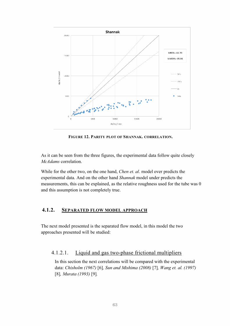
63

FIGURE 12. PARITY PLOT OF SHANNAK. CORRELATION.

As it can be seen from the three figures, the experimental data follow quite closely McAdams correlation.

While for the other two, on the one hand, Chen et. al. model over predicts the experimental data. And on the other hand Shannak model under predicts the measurements, this can be explained, as the relative roughness used for the tube was 0 and this assumption is not completely true.

4.1.2. SEPARATED FLOW MODEL APPROACH

The next model presented is the separated flow model, in this model the two approaches presented will be studied:

4.1.2.1. Liquid and gas two-phase frictional multipliers In this section the next correlations will be compared with the experimental data: Chisholm (1967) [6], Sun and Mishima (2008) [7], Wang et. al. (1997) [8], Murata (1993) [9].

64

FIGURE 13. PARITY PLOT OF CHISHOLM CORRELATION.

FIGURE 14. REPRESENTATION OF 𝝓𝒍𝟐FOR EXPERIMENTAL DATA AND

CHISHOLM MODEL TO XTT.

65

FIGURE 15. PARITY PLOT OF CHISHOLM CORRELATION.

FIGURE 16. REPRESENTATION OF 𝝓𝒍𝟐FOR EXPERIMENTAL DATA AND SUN

AND MISHIMA MODEL TO XTT.

66

FIGURE 17. PARITY PLOT OF WANG ET. AL. CORRELATION.

FIGURE 18. REPRESENTATION OF 𝝓𝒍𝟐FOR EXPERIMENTAL DATA AND WANG

ET. AL. MODEL TO XTT.

67

FIGURE 19. PARITY PLOT OF MURATA CORRELATION.

FIGURE 20. REPRESENTATION OF 𝝓𝒍𝟐FOR EXPERIMENTAL DATA AND

MURATA MODEL TO XTT.

68

Figures 13, 14, 15, 16, 17, 18, 19 and 20 represent the parity plot and the liquid or gas two-phase flow multiplier to the Lockhart-Martinelli parameter. From these figures it can be observed that the correlation that best suits the predicted data is the Chisholm correlation, followed by Sun and Mishima.

Wang et. al. and Murata have bigger deviations. This result can be explained by the conditions in which the correlations where obtained, that do not fit the particular conditions of this experiment. Firstly, Wan et. al. was obtained for refrigerants instead of air-water two-phase flow and the diameter was slightly smaller than the one studied in this thesis. Secondly, for Murata’s correlation forced convective boiling of nonazeotropic mixtures was used, that differs from the experiment conditions of this study.

4.1.3. LIQUID ONLY AND GAS ONLY TWO-PHASE FRICTIONAL MULTIPLIERS.

Now the liquid only/gas only two-phase flow multiplier will be used for comparison by the implementation of the next models: Muller-Steinghagen and Heck (1986) [16] and Tran et. al. (1999) [13].

As it was done in the previous section, parity plots and liquid only two-phase multiplier to Lockhart-Martinelli parameter graphs are presented and collected in Figures 21, 22, 23 and 24.

FIGURE 21. REPRESENTATION OF 𝝓𝒍𝟐FOR EXPERIMENTAL DATA AND

MURATA MODEL TO XTT.

69

FIGURE 22. PARITY PLOT OF MULLER-STEINHAGEN AND HECK CORRELATION.

FIGURE 23. REPRESENTATION OF 𝝓𝒍𝟐FOR EXPERIMENTAL DATA AND TRAN

ET. AL. MODEL TO XTT.

70

FIGURE 24. PARITY PLOT OF TRAN ET. AL. AND HECK CORRELATION.

From the figures, it can be said that Muller-Steinghagen and Heck correlation works better than Tran et. al., also from Table 8 the difference between correlations in MRD and MRAD corroborates the information taken from the graphs.

4.1.4. CONCLUSIONS FOR TWO-PHASE FLOW AIR-WATER INSIDE THE SMOOTH TUBE.

The MRD% and MARD% for all the correlations used in this comparison are presented con Table 8.

As the table shows, the best predictions for the data collected for the particular conditions of this thesis are given by Chisholm and McAdams correlations.

They are closely followed by Muller-Steinghagen and Heck correlation.

71

TABLE 8. MRD% AND MRAD% FOR CORRELATIONS USED IN THE COMPARISON OF TWO-PHASE FLOW AIR-WATER INSIDE THE SMOOTH PIPE.

4.2. MICRO-FIN TUBE:

The pressure drop for single-phase of water and two-phase air-water flow inside the micro-fin tube will be studied.

4.2.1. SINGLE-PHASE WATER FLOW:

As it had been defined in previous section the volume flow rate of water will vary from 50-400 l/h, with steps of 25 l/h.

The data gathered will be analysed and compared with existing correlation and with the data obtained from the single-phase flow of water inside the smooth tube, to study the penalization factor of the insertion of the micro-fins.

4.2.1.1. Obtaining the relative roughness:

Through a comparison of the experimental data with the Haaland formulation [6], already introduced, the relative roughness can be obtained for a later use in the Shannak model for two-phase flow.

As Figure 26 shows, for a sufficiently high Reynolds number (Re > 5000), the experimental friction factor for single-phase flow of water reaches a nearly constant value following the trend of Haaland’s friction factor for a determined relative roughness.

To determine this relative roughness, the three first points obtained are discarded, as their Reynolds number is not sufficiently high, and the flow is characterized by being a slug flow (Figure 25). And for the rest of the

MRD% MARD% McAdams 2.69 19.99 Chen et. al. 85.34 85.34 Shannak -61.79 65.06 Chisholm 5.96 17.15 Sun and Mishima -36.81 36.81 Wang et. al. -45.23 45.23 Murata -49.16 49.16 Muller-Steinghagen and Heck 19.63 21.74 Tran et. al. 54.04 54.04

72

measurements the relative roughness is found accordingly to Haaland’s correlation. Then the average value obtained for this parameter is:

e/D = 0.006863659 with an static deviation of 0.001481.

This number will be used in Shannak’s correlation for two-phase flow of air-water.

FIGURE 25. VISUALIZATION SECTION SHOWING THE SLUG FLOW.

FIGURE 26. REPRESENTATION OF HAALAND FRICTION FACTOR TO THE REYNOLDS NUMBER FOR DIFFERENT RELATIVE ROUGHNESS AND WITH THE EXPERIMENTAL FRICTION FACTOR DATA GATHERED.

Exp. data

Slug

73

4.2.1.2. Penalization factor

The penalization factor, already introduced, takes into account the increase of pressure drop due to the insertion of the micro-fins for the heat transfer enhancement, comparing it to the one that would exist if the tube was smooth:

𝑃𝐹 =(𝑑𝑝𝑑𝑧)9,T9

(𝑑𝑝𝑑𝑧)9,U

( 72)

Where:

𝑃𝐹 [-] Penalization factor; (]^

]_)9,T9 [Pa/m] Frictional pressure drop for the micro-fin tube;

(]^]_)9,U [Pa/m] Frictional pressure drop for the smooth tube;

FIGURE 27. EXPERIMENTAL FRICTION FACTOR FOR SMOOTH TUBE AND MICRO-FIN TUBE TO REYNOLDS NUMBER OF WATER.

Figure 27 presents the experimental friction factor obtained for the smooth and the micro-fin tube. The graph clearly shows the bigger friction factor attained to the flow in the micro-fin tube, that increases with the Reynolds number of water.

74

FIGURE 28. PENALIZATION FACTOR FOR SINGLE-PHASE FLOW OF WATER.

Figure 28 shows the Penalization Factor, some conclusions can be extracted, such as the increase of the Penalization factor with the Reynold number.

Lastly, the mean PF was calculated, obviously excluding the first point that is related to the slug flow (that was already showed in Figure 25).

𝑃𝐹iiii = 1.326 ;

This number will be latter compared to the one obtained for two-phase flow of air-water.

4.2.2. TWO-PHASE FLOW AIR-WATER: This last section of data processing is devoted to air-water flow in the micro-fin tube. The structure used will be the same used for the smooth tube, grouping the correlations according to the models they follow.

4.2.2.1. Homogeneous flow model application: The correlation studied for the comparison with the gathered data of air-water flow is the Shannak correlation.

This correlation was already used for the two-phase flow inside the smooth tube. Now for the micro-fin tube application, a relative roughness has to be consider.

In the single-phase flow of water inside the micro-fin tube a relative roughness of: e/D = 0.006863659 was found applying Haaland’s correlation.

75

Figure 29 shows a good agreement of the correlation with the experimental data, as the MRD% and MARD% are small and nearly all the measurements are positioned within the boundaries bounded by the ± 20 % lines.

FIGURE 29. PARITY PLOT OF SHANNAK’S CORRELATION FOR THE MICRO-FIN TUBE.

4.2.2.2. Separated flow-model approach: Again, the study will be branched in the two different approaches suggested by the separated flow model: liquid/gas two-phase frictional multiplier and liquid only/gas only two-phase frictional multiplier.

i. Liquid/Gas two-phase frictional multipliers correlations: In this section the correlations used for the comparison of the measurements obtained from the two-phase air-water flow inside the micro-fin tube will be: Haraguchi [10], Kedzierski [11] and Murata [9].

Figures 30, 31, 32, 33, 34 and 35 represent the parity plot and the liquid or gas two-phase flow multiplier to the Lockhart-Martinelli parameter.

In the parity plot figures MRD% and MARD% are presented. Comparing these parameters for the three studied models it can be said

76

that, Haraguchi is the best correlation for the approximation of the measurements as it has the smallest MRD% and MRAD%.

For the other two correlations, Kedzierski and Murata, apart from the bigger MRD% and MRAD%, there is another thing that calls the attention, the dispersion in the parity plot.

Both Figures 31 and 33 show that the measurements, even though the MRD% and MRAD% are not so big, don´t follow the trend of the correlation.

Murata’s correlation failure was already expected, as it did not match the two-phase flow in smooth tube. This is because the conditions of Murata’s experiment differ from the ones in this thesis.

While for Kedzierski, the main difference may be found on the different mass fluxes, as his range starts where this thesis ends, again not matching the particular conditions of this work.

FIGURE 30. PARITY PLOT OF HARAGUCHI’S CORRELATION FOR THE MICRO-FIN TUBE.

77

FIGURE 31. REPRESENTATION OF 𝝓𝒍𝟐 FOR EXPERIMENTAL DATA AND HARAGUCHI. MODEL

TO XTT.

FIGURE 32. PARITY PLOT OF KEDZIERSKI’S CORRELATION FOR THE MICRO-FIN TUBE.

78

FIGURE 33. REPRESENTATION OF 𝝓𝒍𝟐FOR EXPERIMENTAL DATA AND KEDZIERSKI MODEL

TO XTT.

FIGURE 34. PARITY PLOT OF MURATA’S CORRELATION FOR THE MICRO-FIN TUBE.

79

FIGURE 35. REPRESENTATION OF 𝝓𝒍𝟐FOR EXPERIMENTAL DATA AND MURATA MODEL TO

XTT.

ii. Liquid/Gas only two-phase frictional multipliers correlations:

In this final comparison section only one correlation will be studied: Cavallini (1999) [14].

FIGURE 36. PARITY PLOT OF CAVALLINI’S CORRELATION FOR THE MICRO-FIN TUBE.

80

This last parity plot shows how Cavallini’s correlation under predicts the experimental data, but even though the MRD% and MARD% are higher than in other correlations the dispersion of the data is very small.

The correlation could be fixed to move the data inside the boundaries delimited by the ± 20% lines.

4.2.3. CONCLUSIONS FOR THE TWO-PHASE FLOW AIR-WATER INSIDE THE MICRO-FIN TUBE COMPARISON: From Table 9 it can be said that the best correlation is Shannak, with (MARD% 16.47), followed by Haraguchi ( MARD% 29.79 ).

TABLE 9. MRD% AND MRAD% FOR CORRELATIONS USED IN THE COMPARISON OF TWO-PHASE FLOW AIR-WATER INSIDE THE MICRO-FIN PIPE.

The rest of the correlations have bigger deviations and so their approach to the measured data is worst. Also as it has been said, some of them are characterized by big dispersions. The fact that Haraguchi’s correlation works for the measurements taken, even though it was developed for boiling two-phase flow, encourages the thesis idea of predicting the pressure drop of boiling and condensation systems by testing adiabatic two-phase flow. This idea came out with the purpose of not having to implement the complex systems that involve testing boiling and condensation pressure drop, which lead to a system characterized by high uncertainties. Instead, adiabatic pressure drop of air-water could be measured, as these type of testing systems require less complexity than the one mentioned before. This assumption was already corroborated by the literature, stating that the pressure drop for diabatic two-phase flow can be taken from adiabatic two-phase flow.

MRD% MARD% Shannak 7.25 16.47 Haraguchi 21.37 29.79 Kedzierski -36.97 45.71 Murata -33.88 45.48 Cavallini -64.93 66.18

81

4.2.4. PENALIZATION FACTOR: As it was done for the single-phase flow, the penalization factor has to be studied to take into account how much do the micro-fins increase the pressure drop inside the tube for the two-phase flow.

For this purpose the data from the two-phase flow inside the smooth tube and micro-fin tube will be used.

First, two graphs are presented to show the pressure drop dependence on the air quality. In these figures, the variation of pressure drop (computed with the model that best fitted de experimental data) with Gtp for different constant qualities is presented. For the smooth tube, the correlation chosen was Muller-Steinghagen and Heck, while for the micro-fin tube Shannak’s correlation was implemented.

From the figures it can be seen that both depend equally, that is, increasing pressure drop for increasing quality (positive relation). Of course the pressure drop of Figure 37 (smooth tube) is smaller than for Figure 38 (micro-fin tube).

FIGURE 37. PRESSURE DROP VARIATION, FOR THE SMOOTH TUBE, WITH GTP FOR DIFFERENT CONSTANT QUALITIES.

FIGURE 38. PRESSURE DROP VARIATION, FOR THE MICRO-FIN TUBE, WITH GTP FOR DIFFERENT CONSTANT QUALITIES.

82

The two pressure drops will be plotted in the same graph for the different volume flow rates of water, to see their variation with Gtp.

FIGURE 39 FIGURE 40

FIGURE 41

FIGURE 42

FIGURE 43 FIGURE 44

83

FIGURES 39, 40, 41, 42, 43, 44, 45, 46, 47 and 48. Pressure drop variation for smooth (s) and micro-fin (mf) tubes with Gtp (mass flux), each one for a different volume flow rate.

The figures above show that, for all the volume flow rates studied the pressure drop inside the micro-fin tube is higher than this one inside the smooth tube. This conclusion was already predicted and what needs to be studied is the proportion of this increase in pressure drop.

The dimensionless increase is measured by the already known PF (Penalization factor).

As it can be observed in Figure 49 the penalization factor, for Gtp high enough, reaches a steady state. This steady state is characterized by a mean value of:

𝑃𝐹iiii = 1.23 with a standard deviation of 0.1.

Recalling information from single-phase water flow section, the average penalization factor in this case was 1.326, which is clearly above the one just calculated for two-phase flow.

This difference will be studied in the next section where the two flows are compared.

FIGURE 45

FIGURE 46

FIGURE 47

FIGURE 48

84

FIGURE 49. PENALIZATION FACTOR FOR THE TWO-PHASE FLOW AIR-WATER.

4.3. SINGLE-PHASE FLOW AND TWO-PHASE FLOW COMPARISON:

As this is the last section of the chapter, the two flows will be compared. The difference in the PF (Penalization Factor) was already presented and will be studied more deeply now.

Figure 50 shows the two penalization factor (single-phase water and two-phase air-water) variation with G.

First of all, it can be seen that the range of mass flux for the two-phase flow (40-440 kg/s/m2) is smaller than the single-phase flow (200-1700 kg/s/m2). This fact, already explained, is due to the limiting condition imposed by the differential pressure transducer, that only allows a maximum measure of 70kPa. As the two-phase flow has a greater pressure drop the range will be narrower.

Secondly, from the plot, it can be observed that the penalization factor for the two-phase flow is smaller than for the water-flow, as the two-phase flow reaches a steady-state, while the single phase flow reaches a minimum around 750 kg/s/m2, and then increases again with G.

The last conclusion favours two-phase flow inside micro-fin tubes as their penalization factor is lower than single-phase flow, which explains the greater use of these tubes in two-phase flows. This doesn´t mean that the pressure drop is higher for single-phase flow, because as it was already said, the pressure drop in the air-water flow is bigger than the water-flow, but

85

means that compared to the smooth tube the increase in pressure drop is higher than for the two-phase.

FIGURE 50. PENALIZATION FACTOR VARIATION WITH G FOR SINGLE-PHASE AND TWO-PHASE FLOW.

86

87

CHAPTER 5:

CONCLUSIONS AND FUTURE DEVELOPMENTS

In this last chapter, the conclusion made throughout the thesis will be presented.

First of all, this work has shown that some correlations work better than others for this particular system. As it was said, the best correlations for the two-phase flow inside the smooth tube were Chisholm and McAdams. While for the micro-fin tube Shannak model was the best approach (using the relative roughness obtained from the single-phase flow).

Secondly, the penalization factor study also gave some information. It could be observed that for both flows the penalization factor reached a more or less constant value. This ratio showed that the average value of the two-phase flow (1.23) was always below the one for the single-phase flow (1.326), which confirms the better performance of the micro-fin tube with the two-phase flow.

To conclude, it has to be said, that more investigation on this subject has to be done, and also on the topics related to it, such as heat transfer coefficient for micro-fin tubes, to obtain the enhancement factor and complete the study of the effect of micro-fins. Actually, further studies will be continued with this micro-fin tube in diabatic flow, where the data obtained in this work will be used for comparison with the new measurements obtained.

88

89

REFERENCES

[1] G. H. Hand book of multiphase systems, 1982.

[2] X. F. X. S. Z. Z. W. C. Yu Xu, “Evaluation of frictional pressure drop correlation for two-phase flow in pipes,” Elsevier, 9 August 2012.

[3] B. A. Shannak, “Frictional pressure drop of gas liquid two-phase flow in pipes,” Nuclear engineering and design 238, 3277-3284 December 2008.

[4] K.-S. Y. C.-C. W. Ing Youn Chen, “Two-phase pressure drop of air-water in small horizontal tubes,” International Journal of Multiphase flow 27, pp. 1293-1299, October 2001.

[5] R. Lockhart and R. M. , “Porposed correlation of Data for Isothermal Two-Phase, Two-Component flow in pipes,” Chemical Engineering Progress, 45, pp. 38-48, 1949.

[6] D. C. “A theoretical basis for the Lockhart-Martinelli correlation for two-phase flow,” International Journal of Heat and Mass Tranfer 10, pp. 1767-1778, July 1967.

[7] K. M. Licheng Sun, “Evaluation analysis of prediction methods for two-phase flow pressure drop in mini-channels,” International Journal of Multiphase flow 35, pp. 47-54, August 2008.

[8] C.-C. Wang, C.-S. Chiang and D.-C. Lu, “Visual observation of two-phase flow pattern of R-22, R-134a, and R-407C in a 6.5-mm smoth tube,” Experimental Thermal and Fluid Sience 15, pp. 395-405, November 1997.

[9] K. M. and K. H. , “Forced Convective boiling of nonazeotropic refrigerant mixtures inside tubes,” Journal of Heat Tranfer 115, pp. 680-690, August 1993.

[10] H. Haraguchi and a. T. F. Shigeru Koyama, “Condensation of refrigerants hcfc 22, hfc 134a and hcfc 123 in a horizontal smooth tube,” Nihon Kikai Gakkai Ronbunshu, B Hen/Transactions of the Japan Society of Mechanical Engineers, Part B, pp. 2111-2116, June 1994.

[11] L. L. J. A. O. a. J. P. M. Mark a. Kedzierski, “Pressure drop during refrigerant condensation inside horizontal smooth, helical micro-fin, and herringbone micro-fin tubes,” Journal Heat Transfer 126(5), pp. 687-696, November 2004.

[12] K. H. Muller-Steinhagen, “A simple friction pressure drop correlation for two-phase flow in pipes,” Chem. Eng. Prog. 20, pp. 297-308.

90

[13] T. C. M. W. M. D. Tran, “Two-phase pressure drop of refrigerants during flow boiling in small channels: an experimental investigation and correlation development,” Journal of multiphase flow 26, pp. 1739-1754, 2000.

[14] D. D. C. L. D. A. Cavallini, “Heat transfer and pressure drop during condensation of refrigerants inside horizontal enhanced tubes.,” International Journal of Refrigeration 23(1), pp. 4-25, January 2000.

[15] “https://www.researchgate.net/publication/313130434_CFD_investigation_of_air-water_separation_using_a_cavity_separator_in_vertical_slug_and_churn_flow/figures?lo=1,” [Online].

[16] H. M.-S. a. K. Heck., “A simple friction pressure drop correlation for two-phase flow in pipes.,” Chemical Engineering and Processing: Peocess Intensification, pp. 297-308, 1986.

[17] Flow condensation pressure drop characteristics of R410A–oil mixture inside small diameter horizontal microfin tubes. [Art].

91

LIST OF FIGURES

FIGURE 1. CUTAWAY VIEW OF THE INSIDE OF A MICRO-FIN TUBE. B) CROSS SECTION OF A

MICRO-FIN TUBE. ............................................................................................................ 25 FIGURE 2. A) CROSS-SECTION OF A TWO-PHASE FLOW INSIDE A TUBE. B) DIFFERENTIAL CROSS-

SECTION AREA 𝐝𝛀OF THE TUBE. ................................................... 30 FIGURE 3. FORCES APPLIED ON A TUBE DIFFERENTIAL. ........................................................... 33 FIGURE 4. REPRESENTATION OF THE SEPARATED FLOW MODEL ............................................... 37 FIGURE 5. FLOW PATTERNS OF TWO-PHASE FLOWS [15] .......................................................... 39 FIGURE 6. REPRESENTATION OF FRICTION FACTOR TO REYNOLD NUMBER FOR DIFFERENT

RELATIVE ROUGHNESS [3] .............................................................................................. 43 FIGURE 7. SCHEME OF THE TYPES OF FINS IN THE MICRO-FIN TUBE. ......................................... 52 FIGURE 8. VISUAL REPRESENTATION OF THE EXPERIMENTAL SYSTEM. 1) WATER CIRCUIT:

ORANGE. 2) AIR CIRCUIT: BLUE. 3)TWO-PHASE FLOW: LIGHT GREY. 4) MIXING SECTION: RED. 5) TEST SECTION: DARK GREY. 6) VISUALIZATION SECTION: GREEN. .......................... 53

FIGURE 9. EXPERIMENTAL FRICTION FACTOR FOR SINGLE-PHASE FLOW. .................................. 60 FIGURE 10. PARITY PLOT OF MCADAMS CORRELATION. ......................................................... 62 FIGURE 11. PARITY PLOT OF CHEN ET. AL. CORRELATION. ...................................................... 62 FIGURE 12. PARITY PLOT OF SHANNAK. CORRELATION. .......................................................... 63 FIGURE 13. PARITY PLOT OF CHISHOLM CORRELATION. .......................................................... 64 FIGURE 14. REPRESENTATION OF 𝝓𝒍𝟐FOR EXPERIMENTAL DATA AND CHISHOLM MODEL TO XTT.

...................................................................................................................................... 64 FIGURE 15. PARITY PLOT OF CHISHOLM CORRELATION. .......................................................... 65 FIGURE 16. REPRESENTATION OF 𝝓𝒍𝟐FOR EXPERIMENTAL DATA AND SUN AND MISHIMA MODEL

TO XTT. ........................................................................................................................... 65 FIGURE 17. PARITY PLOT OF WANG ET. AL. CORRELATION. ..................................................... 66 FIGURE 18. REPRESENTATION OF 𝝓𝒍𝟐FOR EXPERIMENTAL DATA AND WANG ET. AL. MODEL TO

XTT................................................................................................................................. 66 FIGURE 19. PARITY PLOT OF MURATA CORRELATION.............................................................. 67 FIGURE 20. REPRESENTATION OF 𝝓𝒍𝟐FOR EXPERIMENTAL DATA AND MURATA MODEL TO XTT.67 FIGURE 21. REPRESENTATION OF 𝝓𝒍𝟐FOR EXPERIMENTAL DATA AND MURATA MODEL TO XTT.68 FIGURE 22. PARITY PLOT OF MULLER-STEINHAGEN AND HECK CORRELATION. ....................... 69 FIGURE 23. REPRESENTATION OF 𝝓𝒍𝟐FOR EXPERIMENTAL DATA AND TRAN ET. AL. MODEL TO

XTT................................................................................................................................. 69 FIGURE 24. PARITY PLOT OF TRAN ET. AL. AND HECK CORRELATION. ..................................... 70 FIGURE 25. VISUALIZATION SECTION SHOWING THE SLUG FLOW. ............................................ 72 FIGURE 26. REPRESENTATION OF HAALAND FRICTION FACTOR TO THE REYNOLDS NUMBER FOR

DIFFERENT RELATIVE ROUGHNESS AND WITH THE EXPERIMENTAL FRICTION FACTOR DATA

GATHERED. .................................................................................................................... 72 FIGURE 27. EXPERIMENTAL FRICTION FACTOR FOR SMOOTH TUBE AND MICRO-FIN TUBE TO

REYNOLDS NUMBER OF WATER. ...................................................................................... 73

92

FIGURE 28. PENALIZATION FACTOR FOR SINGLE-PHASE FLOW OF WATER. ................................ 74 FIGURE 29. PARITY PLOT OF SHANNAK’S CORRELATION FOR THE MICRO-FIN TUBE. ................. 75 FIGURE 30. PARITY PLOT OF HARAGUCHI’S CORRELATION FOR THE MICRO-FIN TUBE............... 76 FIGURE 31. REPRESENTATION OF 𝝓𝒍𝟐 FOR EXPERIMENTAL DATA AND HARAGUCHI. MODEL TO

XTT................................................................................................................................. 77 FIGURE 32. PARITY PLOT OF KEDZIERSKI’S CORRELATION FOR THE MICRO-FIN TUBE. ............. 77 FIGURE 33. REPRESENTATION OF 𝝓𝒍𝟐FOR EXPERIMENTAL DATA AND KEDZIERSKI MODEL TO

XTT................................................................................................................................. 78 FIGURE 34. PARITY PLOT OF MURATA’S CORRELATION FOR THE MICRO-FIN TUBE.................... 78 FIGURE 35. REPRESENTATION OF 𝝓𝒍𝟐FOR EXPERIMENTAL DATA AND MURATA MODEL TO XTT.

...................................................................................................................................... 79 FIGURE 36. PARITY PLOT OF CAVALLINI’S CORRELATION FOR THE MICRO-FIN TUBE. ............... 79 FIGURE 37. PRESSURE DROP VARIATION, FOR THE SMOOTH TUBE, WITH GTP FOR DIFFERENT

CONSTANT QUALITIES. .................................................................................................... 81 FIGURE 38. PRESSURE DROP VARIATION, FOR THE MICRO-FIN TUBE, WITH GTP FOR DIFFERENT

CONSTANT QUALITIES. .................................................................................................... 81 FIGURE 39............................................................................................................................. 82 FIGURE 40............................................................................................................................. 82 FIGURE 41............................................................................................................................. 82 FIGURE 42............................................................................................................................. 82 FIGURE 43............................................................................................................................. 82 FIGURE 44............................................................................................................................. 82 FIGURE 45............................................................................................................................. 83 FIGURE 46............................................................................................................................. 83 FIGURE 47............................................................................................................................. 83 FIGURE 48............................................................................................................................. 83 FIGURE 49. PENALIZATION FACTOR FOR THE TWO-PHASE FLOW AIR-WATER. ........................... 84 FIGURE 50. PENALIZATION FACTOR VARIATION WITH G FOR SINGLE-PHASE AND TWO-PHASE

FLOW. ............................................................................................................................ 85

93

LIST OF TABLES

TABLE 1. CONSTANT VARIATION WITH FLOW REGIME. ............................................................ 44 TABLE 2. FORMULATION OF FRICTION FACTOR FOR CAVALLINI CORRELATION. ....................... 49 TABLE 3. GEOMETRIC CHARACTERISTICS OF THE SMOOTH TUBE. ............................................ 52 TABLE 4. GEOMETRIC CHARACTERISTICS OF THE MICRO-FIN TUBE .......................................... 52 TABLE 5. INSTRUMENTATION UNCERTAINTIES. ....................................................................... 54 TABLE 6. OPERATING CONDITIONS OF THE EXPERIMENT. ........................................................ 55 TABLE 7. MRD AND MARD RELATED TO THE EXPERIMENTAL WATER FRICTION FACTOR IN A

SMOOTH TUBE. ............................................................................................................... 60 TABLE 8. MRD% AND MRAD% FOR CORRELATIONS USED IN THE COMPARISON OF TWO-PHASE

FLOW AIR-WATER INSIDE THE SMOOTH PIPE. .................................................................... 71 TABLE 9. MRD% AND MRAD% FOR CORRELATIONS USED IN THE COMPARISON OF TWO-PHASE

FLOW AIR-WATER INSIDE THE MICRO-FIN PIPE. ................................................................ 80

94

95

SYMBOLS

Latin symbols:

𝐴 [m2] Actual cross-sectional flow are of the tube. 𝐴 [-] Constants depending on the model.

𝐴ä [m2] Cross-sectional area taking into account the variations due to the fins.

𝐴ã [m2] The nominal flow area based on the fin-root diameter

𝐵𝑜 [-] Bond number.

D [m] Diameter.

De [m] Equivalent diameter.

Di [m] Internal diameter.

𝐸 [-] Enhancement factor;

𝑓c [-] Liquid friction factor.

𝑓c® [-] Liquid only friction factor.

𝑓b [-] Gas friction factor.

𝑓b® [-] Gas only friction factor.

𝑓¢^ [-] Two-phase friction factor.

g [m/s2] Gravitational acceleration.

𝐺c [kg/m2/s] Actual mass flux for liquid.

𝐺∗c [kg/m2/s] Apparent mass flux for liquid.

𝐺b [kg/m2/s] Actual mass flux for gas.

𝐺∗b [kg/m2/s] Apparent mass flux for gas.

ℎ [m] Fin height.

ℎT9 [W/m2K] Micro-fin tube heat transfer coefficient.

ℎU [W/m2K] Smooth tube heat transfer coefficient.

𝚥 ̅ [m/s] Mixture velocity.

𝑗c [m/s] Superficial velocity for the liquid.

𝚥c̅ [m/s] Cross-section average superficial velocity for the gas.

𝑗b [m/s] Superficial velocity for the gas.

𝚥b̅ [m/s] Cross-section average superficial velocity for the liquid.

𝐿𝑎 [-] Laplace number.

m [-] Constant depending on the model.

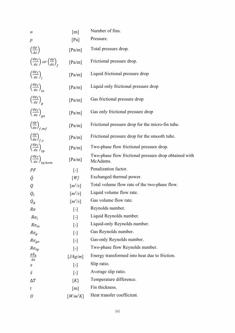
96

n [m] Number of fins.

p [Pa] Pressure.

B]^]_G [Pa/m] Total pressure drop.

B]^¦]_G or B]^

]_G9

[Pa/m] Frictional pressure drop.

B]^¦]_Gc [Pa/m] Liquid frictional pressure drop

B]^¦]_Gc®

[Pa/m] Liquid only frictional pressure drop

B]^¦]_Gb

[Pa/m] Gas frictional pressure drop

B]^¦]_Gb®

[Pa/m] Gas only frictional pressure drop

B]^]_G9,T9

[Pa/m] Frictional pressure drop for the micro-fin tube.

B]^]_G9,U

[Pa/m] Frictional pressure drop for the smooth tube.

B]^¦]_G¢^ [Pa/m] Two-phase flow frictional pressure drop.

B]^¦]_G¢^,¾®T

[Pa/m] Two-phase flow frictional pressure drop obtained with McAdams.

𝑃𝐹 [-] Penalization factor.

�̇� [W] Exchanged thermal power.

𝑄 [m3/s] Total volume flow rate of the two-phase flow.

𝑄c [m3/s] Liquid volume flow rate.

𝑄b [m3/s] Gas volume flow rate.

𝑅𝑒 [-] Reynolds number.

𝑅𝑒c [-] Liquid Reynolds number.

𝑅𝑒c® [-] Liquid-only Reynolds number.

𝑅𝑒b [-] Gas Reynolds number.

𝑅𝑒b® [-] Gas-only Reynolds number.

𝑅𝑒¢^ [-] Two-phase flow Reynolds number. ]Ki¡]_

[J/kg/m] Energy transformed into heat due to friction.

𝑠 [-] Slip ratio.

�̅� [-] Average slip ratio.

Δ𝑇 [K] Temperature difference.

t [m] Fin thickness.

𝑈 [W/m2K] Heat transfer coefficient.

97

𝑢c [m/s] Local velocity for the liquid.

𝑢cy [m/s] Cross-section average velocity for the gas.

𝑢b [m/s] Local velocity for the gas.

𝑢biii [m/s] Cross-section average velocity for the gas.

𝑣Tiiii [m3/kg] Momentum weighted specific volume.

𝑊𝑒 [-] Weber number.

𝑋 [-] Lock-hart Martinelli parameter.

𝑥 [-] Air mass quality.

�̅� [-] Average mass quality.

Greek symbols:

𝛼 [-] Void fraction.

𝛼i [-] Average void fraction.

b [-] Helix angle of the fins.

Γ [kg/s] Total mass flow rate of the two-phase flow.

Γc [kg/s] Liquid mass flow rate.

Γb [kg/s] Gas mass flow rate.

𝜙c� [-] Liquid two-phase multiplier.

𝜙c®� [-] Liquid only two-phase multiplier.

𝜙b� [-] Gas two-phase multiplier.

𝜙b®� [-] Gas only two-phase multiplier.

𝜇 [kg/m/s] Viscosity.

�̅� [kg/m/s] Two-phase viscosity.

𝜇c [kg/m/s] Liquid viscosity.

𝜇b [kg/m/s] Gas viscosity.

𝜌 [kg/m3] Density.

𝜌∗ [kg/m3] Photographic density. 𝜌~ [kg/m3] Bulk density.

𝜌c [kg/m3] Liquid density.

𝜌b [kg/m3] Gas density.

𝜎 [N/m] Surface tension.

𝜏 [Pa] Sheer stress.

98

Ω [m3] Total cross-section area.

W [-] Parameter depends on Bond number.

Ωc [m3] Liquid cross-section area.

Ωb [m3] Gas cross-section area.

99

SUBSCRIPTS

1 = position z.

2 = position z+dz.

a = Accelerative term.

e = equivalent.

f = Frictional term.

g = Gravitational term.

g = gas

l = liquid.

s = Perimeter of the cross-section.