Embed Size (px)
DESCRIPTION
Pricing Maturity Guarantee with Dynamic Living Benefit. 숭실대학교 정보통계 보험수리학과 고방원 [email protected]. I-1. Dynamic Fund Protection. 풋옵션을 업그레이드한 보증유형 (A Strengthened Version of Put Option) 계약기간 동안 펀드 계좌의 금액이 보증수준 K 이하로 떨어지지 않도록 보증 펀드 계좌의 금액이 K 이하가 되면 보증 판매자는 적당한 금액을 즉시 펀드에 추가하도록 설계 - PowerPoint PPT Presentation
Citation preview

I-1. Dynamic Fund Protection
• 풋옵션을 업그레이드한 보증유형 (A Strengthened Version of Put Option)
- 계약기간 동안 펀드 계좌의 금액이 보증수준 K 이하로 떨어지지 않도록 보증
- 펀드 계좌의 금액이 K 이하가 되면 보증 판매자는 적당한 금액을 즉시 펀드에 추가하도록 설계
- 흔히 Reset Guarantee 라 불림

I-2. Dynamic Fund Protection
• F(t) : 시간 t 에서의 unprotected 펀드계좌의 잔고
• 시간 t 에서의 DFP 펀드계좌의 잔고
•
:)(~
tF
Protection Level K
Time t
)(~
tF
F(t)
F(0)
I-3. Dynamic Fund Protection
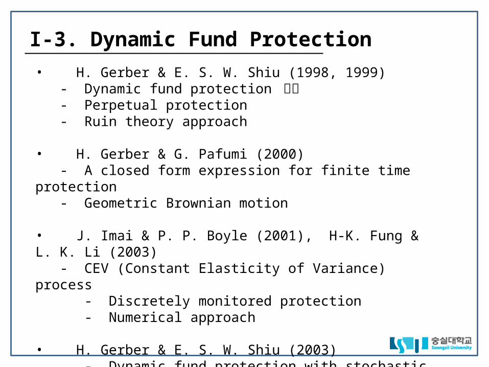
• H. Gerber & E. S. W. Shiu (1998, 1999) - Dynamic fund protection 도입- Perpetual protection- Ruin theory approach
• H. Gerber & G. Pafumi (2000) - A closed form expression for finite time protection- Geometric Brownian motion
• J. Imai & P. P. Boyle (2001), H-K. Fung & L. K. Li (2003)- CEV (Constant Elasticity of Variance) process
- Discretely monitored protection- Numerical approach
• H. Gerber & E. S. W. Shiu (2003)- Dynamic fund protection with stochastic barrier- Optimal exercise strategy
I-4. Dynamic Fund Protection
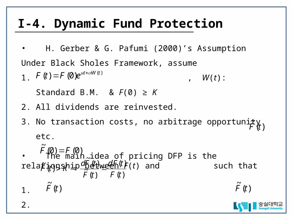
• H. Gerber & G. Pafumi (2000)’s Assumption
Under Black Sholes Framework, assume
1. , W(t): Standard B.M. & F(0) ≥ K
2. All dividends are reinvested.
3. No transaction costs, no arbitrage opportunity etc.
• The main idea of pricing DFP is the relationship between F(t) and such that
1.
2.
3. If drops to K, just enough money will be added so that
does not fall below K.
)()0()( tWteFtF
)(~
tF
)0()0(~
FF
)(
)(
)(~
)(~
)(~
tF
tdF
tF
tFdKtF
)(~
tF )(~
tF

I-5. Dynamic Fund Protection
More precisely,
Why?
1. Consider as the number of fund units.
2. Note that n(0) = 1 & n(t) is nondecreasing.
3.
4. The equal sign is chosen to minimize the guarantee cost.
See Gerber & Shiu (2003).
)(
max,1max)()(~
0 sF
KtFtF
ts
tssF
KsntsKsnsFsF 0,
)()(0,)()()(
~
)(max)(0 sF
Ksn
ts
)(
max,1max)(0 sF
Ktn
ts

I-6. Dynamic Fund Protection
• An interpretation of the process
Consider when
After simple algebra,
By Graversen and Shiryaev (2000), we recognize as
a reflecting Brownian motion with drift = μ, volatility = σ, started at
0)(~
ttF
0
)(~
ln
tK
tF.)0()( )(tWteFtF
.)(max,)0(
lnmax)()(
~ln
0
sWs
K
FtWt
K
tFts
0
)(~
ln
tK
tF
.)0(
lnK
F

I-7. Dynamic Fund Protection
• A useful result about a reflecting B. M. with drift from Graversen and
Shiryaev (2000)
For any
where satisfies the stochastic differential equation
• Sometimes, |μt + W(t)| is called a reflecting B. M. with drift.
,)()(max,max)(0
tYsWsytWtlaw
ts
,, RR y
0)( ttY
.)0(),()(sign)( yYtdWdttYtdY

( )t W t
0 0
)(max,max0
sWsyts
y y
I-8. Dynamic Fund Protection
)(tY
t t

I-9. Dynamic Fund Protection
• For a reflecting B. M. with drift, an explicit expression of the transi-
tion density is available.
- See Cox & Miller (1965) for the derivation.
Let denote the probability that a reflecting B.M.
started at will be observed in the interval between x and
x + dx after time T.
dxTK
Fxp
,)0(
ln;
K
F )0(ln
T
TKFxe
TTK
Fxn
F
KTT
K
FxnT
K
Fxp
x
/)0(ln1
2
,)0(
ln;)0(
,)0(
ln;,)0(
ln;
2
2
2
2
2
2
2

I-10. Dynamic Fund Protection
• Pricing formula for DFP – Gerber & Pafumi (2000)
By the fundamental theorem of asset pricing,
And,
After some tedious calculation, one may obtain the following formula:
cost. guarantee DFP)0()(~
EQ FTFe rT
.,)0(
ln;E)(~
E0
/)(~
lnQQ
dxT
K
FxpeKeeKeTFe xrTKTFrTrT

I-11. Dynamic Fund Protection
• Pricing formula for DFP – Gerber & Pafumi (2000)
T
TFKe
rKe
T
TeF
K
F
KrK
T
TeF
K
F
KrK
T
TFKe
FT
TFKe
rKe
rT
rTrT
r
rTr
rTrT
rT
22
22
2
22
2
222
21
)0(ln
221
)0(ln
)0(
2
Price)Put Scholes-(Black BSP
21
)0(ln
)0(
2
21
)0(ln
)0(21
)0(ln
21cost guarantee DFP
2
2

I-12. Dynamic Fund Protection
• Esscher Transform
Discussion paper by Y-C. Huang and E. S. W. Shiu (2000, NAAJ) derives
the pricing formula by using the reflection principle and the method
of Esscher Transforms.

I-13. Dynamic Fund Protection
• Numerical Illustration – Table 3 from Gerber & Pafumi (2000)
When F(0) = 100, T = 1, σ = 0.2, r = 0.04
• Interesting Fact
One may verify that
K 80 85 90 95 100
European Put Price 0.7693 1.4654 2.5315 4.0325 6.0040
DFP Price 1.7709 3.4239 6.0120 9.7476 14.7931
Ratio 2.30 2.34 2.37 2.42 2.46
.)0(any for 2BSP
Price Guarantee DFPlim
0KF
T

II-1. Maturity Guarantee with DLB
• Maturity Guarantee with Dynamic Living Benefit 의 제안
- 펀드의 잔고가 미리 정한 일정 수준 (B) 을 넘어가면 그 초과액을 고객에게 배당금과 같은 형태로 바로 지급하고 만약 만기일에 펀드잔고가 보장수준 (K) 이하로 떨어지면 부족한 부분을 보장
• Maturity Guarantee with Dynamic Living Benefit 의 제안 배경
- 변액연금에서 GLB (Guaranteed Living Benefit) 상품인 GMWB, GMIB, GMAB 의 선택비율이 높음
- Dynamic Fund Protection 의 쌍대 (Dual) 문제로 명시적 가격 결정공식 유도가 가능
- B 와 K 를 동시에 조정 , Dynamic Fund Protection 보다 Cheap

F(0)
Protection Level K
Deficit covered by protection issuer
B
DLB payment level
II-2. Maturity Guarantee with DLB

II-3. Maturity Guarantee with DLB
• F(t) : 시간 t 에서의 펀드계좌의 잔고
• 시간 t 에서의 DLB 를 지급하는 펀드계좌의 잔고
• F(t) 와 의 관계식
이 성립함
:)(ˆ tF
)(ˆ tF
)(
min,1min)()(ˆ0 sF
BtFtF
ts

II-4. Maturity Guarantee with DLB
• Under the same framework with Gerber and Pafumi (2000),
1.
2. 0 < K ≤ F(0) = 1 ≤ B
3. Denote k = ln K, b = ln B (k ≤ 0 ≤ b)
4. VL(B, T): time-0 value of the aggregate DLB payments
5. VP(K, B, T): time-0 value of the maturity guarantee with payoff
6. Investor pays 1 + VP(K, B, T) at the beginning of the contract.
)(ˆ tFK
1)0( F

II-5. Maturity Guarantee with DLB
• Similarly in DFP,
Thus, the process is a reflecting B. M. started at b with
drift (– μ), volatility σ, and reflecting barrier at 0.
• The pricing formulas for VL(B, T) and VP(K, B, T) can be found
by using the transition density.
.)(max,max)()(ˆ
ln0
sWsbtWttF
Bts
)(ˆ/ln tFB
II-6. Maturity Guarantee with DLB
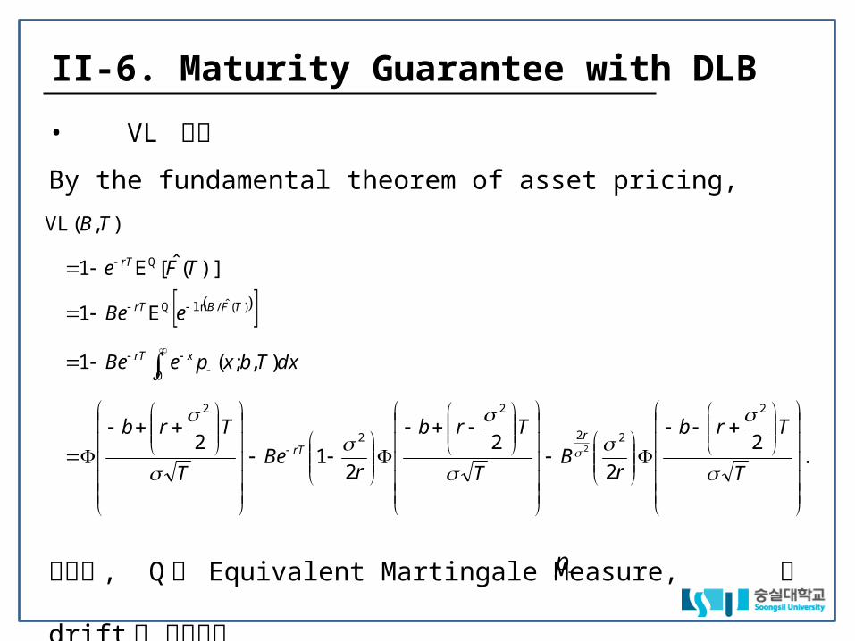
• VL 공식
By the fundamental theorem of asset pricing,
여기서 , Q 는 Equivalent Martingale Measure, 은 drift 가
반대부호
.2
2
2
21
2
),;(1
E1
)](ˆ[E1
),(VL
2
22
2
2
2
0
)(ˆ/lnQ
Q
2
T
Trb
rB
T
Trb
rBe
T
Trb
dxTbxpeBe
eBe
TFe
TB
rrT
xrT
TFBrT
rT
p

II-7. Maturity Guarantee with DLB
• VP 공식
T
Trbk
rB
T
Trbk
re
B
KK
T
Trk
T
Trk
Ke
dxTbxpBeKe
BeKeTFKe
TBK
rrT
r
rT
KB
xrT
TFBrTrT
2
2
2
22
2
22
),;(
E)(ˆE
),,(VP
2
212
2
212
22
)/ln(
)(ˆ/lnQQ
22

II-8. Maturity Guarantee with DLB
• In the derivation of the pricing formulas, we have used two extensions from
Gerber and Pafumi (2000, NAAJ):
• Similarly with DFP,
Because VP ≥ BSP, the sum of the last terms should always be positive.
.11
1
,,;
22
22
2
1
22
12
ae
c
ae
cdx
xe
caedxxne
ccac
a
cx
cc
a
cx
T
Trbk
rB
T
Trbk
re
B
KKTBK
rrT
r
22
2
22
2BSP),,(VP
2
212
2
212
22

II-9. Maturity Guarantee with DLB
• The pricing formulas can be derived by using the method of Esscher
Transforms.
• The pricing formulas can be easily extended to the case with exponen-
tially varying barriers.

• Numerical Illustration – 1 (r = 5%, σ = 20%)
0
0.2
0.4
0.6
0.8
1.0
20 40 60 80 Maturity (Years)
: B = 1.0
: B = 1.5
: B = 2.0
: B = 2.5
II-10. Maturity Guarantee with DLB
VL(B, T)

0
0.02
0.04
0.06
0.08
20 40 60 80 Maturity (Years)
0.10 K = 1.0
K = 0.9
K = 0.8
K = 0.7
K = 0.6
• Numerical Illustration – 2 (r = 5%, σ = 20%)
II-11. Maturity Guarantee with DLB
VP(K, B, T)
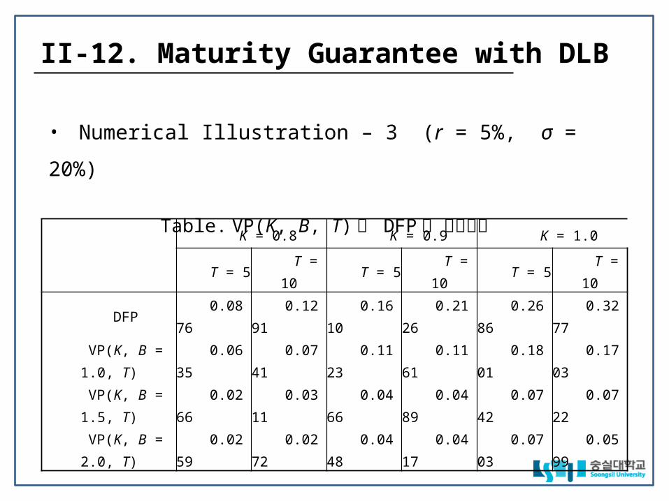
• Numerical Illustration – 3 (r = 5%, σ = 20%)
Table. VP(K, B, T) 와 DFP 의 가격비교
K = 0.8 K = 0.9 K = 1.0
T = 5 T = 10 T = 5 T = 10 T = 5 T = 10
DFP 0.0876 0.1291 0.1610 0.2126 0.2686 0.3277
VP(K, B = 1.0, T) 0.0635 0.0741 0.1123 0.1161 0.1801 0.1703
VP(K, B = 1.5, T) 0.0266 0.0311 0.0466 0.0489 0.0742 0.0722
VP(K, B = 2.0, T) 0.0259 0.0272 0.0448 0.0417 0.0703 0.0599
II-12. Maturity Guarantee with DLB

0
1
2
3
4
Maturity (Years)8 12 16
B = 1.2
B = 1.1
B = 1.0
: K = 1.0
: K = 0.9
: K = 0.8
• Numerical Illustration – 4 (r = 5%, σ = 20%)
VP(K, B, T) 와 European Put Price 의 가격비
II-13. Maturity Guarantee with DLB

II-14. Maturity Guarantee with DLB
• Asymptotic Result
By the asymptotic formula in Abramowitz and Stegun (1972), it can
be shown that for 0 < K ≤ 1,
.1),(BSP
),1,(VPlim
,2),(BSP
),1,(VPlim
0
0
TK
TBK
TK
TBK
T
T

0
0.1
1 2 3 4
0.2
0.3
0.4
K = 1.0
K = 0.9
K = 0.8
VL(B, T = 5)
VP(K, B, T = 5)
B
Break-even if B = 2.01
• Numerical Illustration – 5 (r = 5%, σ = 20%)
II-15. Maturity Guarantee with DLB

II-16. Maturity Guarantee with DLB
• Future Research
1. For reflected processes more general than Brownian Motion, see Linetsky (2005).
2. What if reflection is replaced by refraction? See, for example, Gerber & Shiu
(2006).
Withdrawal Level
Protection Level

참고문헌
• Abramowitz, M. and Stegun, I. (1972) Handbook of Mathematical Functions. Dover
Publications: New York
• Cox, D. R. and Miller, H. (1965) The Theory of Stochastic Processes. Chapman &
Hall
• Fung, H-K. and Li, L. K. (2003) Pricing Discrete Dynamic Fund Protections. North
American Actuarial Journal 7(4): 23-31.
• Graversen, S. E. and Shiryaev, A. N. (2000) An Extension of P. Lévy’s Distributional
Properties to the Case of a Brownian Motion with Drift. Bernoulli 6(4): 615-620.
• Gerber, H. U. and Pafumi, G. (2000) Pricing Dynamic Investment Fund Pro-
tection. North American Actuarial Journal 4(2): 28-37. Discussion Paper by
Huang, Y-C. & Shiu, E. S. W.

• Gerber, H. U. and Shiu, E. S. W. (1998) Pricing Perpetual Options for Jump
Processes. North American Actuarial Journal 2(3): 101-107.
• Gerber, H. U. and Shiu, E. S. W. (1999) From Ruin Theory to Pricing Reset
Guarantees and Perpetual Put Options. Insurance: Mathematics and Econom-
ics 24(1): 3-14.
• Gerber, H. U. and Shiu, E. S. W. (2003) Pricing Perpetual Fund Protection with
Withdrawal Option. North American Actuarial Journal 7(2): 60-92.
• Gerber, H. U. and Shiu, E. S. W. (2006) On Optimal Dividends: From Reflection
to Refraction. Journal of Computational and Applied Mathematics 186: 4-22.
• Imai, J. and Boyle, P. P. (2001) Dynamic Fund Protection. North American Actuarial
Journal 5(3): 31-51.
• Linetsky, V. (2005) On the Transition Densities for Reflected Diffusions. Advances
in Applied Probability 37: 435-460.