Quantum State Tomographyof the 6 qubit photonic symmetric Dicke State

Alexander Niggebaum

München 2011

Quantum State Tomographyof the 6 qubit photonic symmetric Dicke State

Alexander Niggebaum

Masterarbeit

an der Fakultät für Physik

der Ludwig�Maximilians�Universität

München

vorgelegt von

Alexander Niggebaum

aus Fürstenfeldbruck

München, den 27.10.2011

Written in the group of Prof. Dr. Harald Weinfurter

Contents

1 Introduction 1

2 State description in quantum mechanics 3

2.1 Quantum mechanical states . . . . . . . . . . . . . . . . . . . . . . . . . . 3

2.1.1 Multipartite states . . . . . . . . . . . . . . . . . . . . . . . . . . . 5

2.1.2 Entanglement . . . . . . . . . . . . . . . . . . . . . . . . . . . . . . 6

2.1.3 Density matrices . . . . . . . . . . . . . . . . . . . . . . . . . . . . 6

2.1.3.1 Structure of a density matrix . . . . . . . . . . . . . . . . 8

2.1.3.2 Entanglement between systems . . . . . . . . . . . . . . . 9

2.1.4 Measures . . . . . . . . . . . . . . . . . . . . . . . . . . . . . . . . . 9

2.2 Measurements . . . . . . . . . . . . . . . . . . . . . . . . . . . . . . . . . . 10

2.3 Measuring photonic qubits . . . . . . . . . . . . . . . . . . . . . . . . . . . 12

3 Quantum State Tomography 15

3.1 Tomography of a single qubit . . . . . . . . . . . . . . . . . . . . . . . . . 15

3.2 Multiqubit Tomography . . . . . . . . . . . . . . . . . . . . . . . . . . . . 17

3.3 Permutationally Invariant Quantum State Tomography . . . . . . . . . . . 19

4 Maximum Likelihood Estimation 27

5 Experiment 31

5.1 Entangled State Production via Spontaneous Parametric Down Conversion 31

5.2 The Symmetric Dicke State . . . . . . . . . . . . . . . . . . . . . . . . . . 33

5.3 Production of a Symmetric Dicke State . . . . . . . . . . . . . . . . . . . . 34

5.4 Higher order noise of D36 . . . . . . . . . . . . . . . . . . . . . . . . . . . . 37

5.5 Laser System . . . . . . . . . . . . . . . . . . . . . . . . . . . . . . . . . . 39

6 State Tomography of the 6 qubit symmetric Dicke State 45

6.1 Symmetric Overlap . . . . . . . . . . . . . . . . . . . . . . . . . . . . . . . 45

6.2 Reconstructed density matrices . . . . . . . . . . . . . . . . . . . . . . . . 46

6.3 Fidelity . . . . . . . . . . . . . . . . . . . . . . . . . . . . . . . . . . . . . 51

6.4 Noise analysis . . . . . . . . . . . . . . . . . . . . . . . . . . . . . . . . . . 51

ii CONTENTS

7 Alignment Errors 557.1 Symmetry of |Φ+〉 . . . . . . . . . . . . . . . . . . . . . . . . . . . . . . . . 587.2 Reconstructed o�sets for measured data . . . . . . . . . . . . . . . . . . . 607.3 E�ects on Eigenvalues and Fidelity . . . . . . . . . . . . . . . . . . . . . . 627.4 Summary . . . . . . . . . . . . . . . . . . . . . . . . . . . . . . . . . . . . 62

8 Conclusion and Outlook 63

A Overlap with the symmetric subspace 65

B Density matrix contributions 69

C Counts for |Ψ+〉 = 1√2

(|HH〉+ |VV〉) 71

D Symmetries 73D.1 The 2 qubit symmetric Dicke State . . . . . . . . . . . . . . . . . . . . . . 73D.2 The Bell States . . . . . . . . . . . . . . . . . . . . . . . . . . . . . . . . . 74

E Additional simulation results 75

F Additional density matrices 77

Nomenclature

APD Avalanche Photo Diode

BBO β-Barium-Borate. Crystal material used to create entangled photons in Sponta-neous Parametric Down Conversion (SPDC)

CW Continuous Wave (Laser)

FPGA Field Programmable Gate Array

HWP Half Wave Plate or λ2plate

LBO Lithium Triborate. Crystal used for upconversion.

MLE Maximum Likelihood Estimation

PBS Polarizing Beam Splitter

PI Permutationally Invariant

QWP Quarter Wave Plate or λ4plate

SPDC Spontaneous Parametric Down Conversion

iv CONTENTS

1 Introduction

Entanglement of particles or systems has been widely investigated in recent years[15, 25,42]. Small 2 qubit systems are easy to produce and observe. Entanglement itself becomesvisible if the system is well isolated from external in�uences. Otherwise interaction with theenvironment will lead to what is called decoherence and is the generic term for quantummembers loosing coherency by interaction with other systems that are not part of theinvestigation. Thus isolation is crucial. In case of atoms this can be done in magneto opticaltraps[30] where counter propagating laser beams along the generic three dimensional axesin combination with a magnetic �led gradient are used. Experimental requirements arein general very high[36]. A convenient system consists of photons because of no e�ectiveinteraction among each other and easy production in large quantities. Any quantum statehowever is destroyed during a measurement because the photon must be absorbed in theactive material of the detector to generate an electric pulse. There are schemes thatdemonstrate the realization of quantum non demolition measurements on photons[32] butperformance is still not optimal compared to destructive methods. If the state is notsubject to reutilization, standard techniques su�ce.

A problem with larger systems is the increasing number of parameters needed to de-scribe it. Full information include relations between every member with each other. Tomeasure the state of a system, generic schemes were developed[22]. For reliable informa-tion of every parameter in the system, su�cient amount of data need to be collected, sothe overall measurement time increases as well. In addition, most multiqubit states areeither hard to create or store, so measurement time must be kept as short and e�ective aspossible. In this thesis the general tomographic scheme for qubit quantum systems will beintroduced. In a bright laser system the Symmetric Dicke State[11] consisting of 6 pho-tonic qubits, each entangled with every other, can be created and observed. Experimentalconditions impose low production rates that render the generic approach impossible.

Permutational invariant state tomography, a scheme that exploits the symmetry of thestate is used to reduce the amount of data needed for reconstruction. Time and amountof data can be reduced by 96.2% while still reproducing full information on the state. Ana priori check ensures that the state follows the necessary symmetry. Gathered data canbe reused in the later process. This makes permutational invariant tomography highlye�ective on symmetric states.

2 1. Introduction

2 State description in quantum me-

chanics

In this work, experimental creation and observation of a genuine 6 partite entangled stateare described. The basic framework to describe quantum mechanical states will be summa-rized in this chapter. In addition, basic measures used to compare measured with theoret-ically expected states are motivated. The choice of topics relies on aspects needed for thelater description of the experiment; in depth derivation and also motivation of the mathe-matical framework of quantum mechanics are presented in textbooks, e.g. [34, 18, 12, 38].

2.1 Quantum mechanical states

In analogy to the basic unit of information in computer science, the state of a quantumsystem is called a �quantum bit� or short �qubit�, as coined by Schumacher[37]. Likeits digital analogue it is a 2 level system that can be in the excited or unexcited state.Implementations can vary, dependent the carrier system chosen1. Basic requirement forall is long time stability to perform operations with the bits or even store them. Somesystems are better suited to meet this prerequisite, other require great experimental e�ort(e.g. trapped ions).

In contrast to a bit, a qubit can exist in superposition of its two states. However asingle readout will show it to be in either one state. Consecutive measurements will mapthe superposition on the recorded statistics2, but the individual outcome is not predictable.For their nonexistent interaction with each other and easy experimental implementation,photons are used here. We de�ne horizontal polarization as the excited |H〉 and verticalpolarization |V〉 as the unexcited state. The general superposition reads

|ψ〉 = cos

(θ

2

)|H〉+ eiφ sin

(θ

2

)|V〉

1For example ions use metastable atom levels and superconducting qubits the �ux quantization ofsquids[7].

2For example from 100 measurements, 50 will result in the excited, 50 in the unexcited state, leading tothe conclusion that the qubit was in a 50/50 superposition. This deduction is made under the assumptionthat the qubit can be created in the same state over and over again, if the readout process changes thesystems state.

4 2. State description in quantum mechanics

where the angle θ can be seen as the mixture of |H〉 and |V〉, φ as the phase between them.Any vectors or matrices are written in the |H〉, |V〉 basis, if not stated otherwise. In vector

representation they are chosen |H〉 =

(10

)and |V〉 =

(01

). Other polarization states

can be expressed through these

|P〉 =1√2

(|H〉+ |V〉)

|M〉 =1√2

(|H〉 − |V〉)

|R〉 =1√2

(|H〉+ i|V〉)

|L〉 =1√2

(|H〉 − i|V〉)

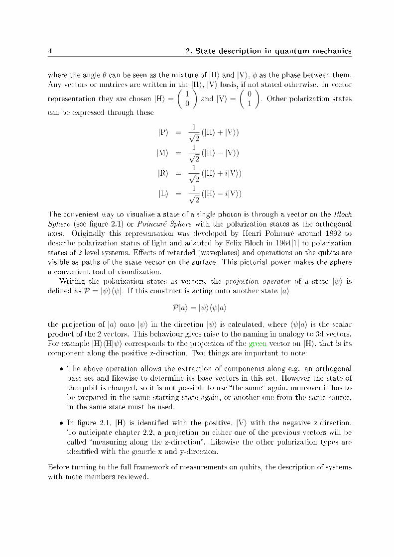
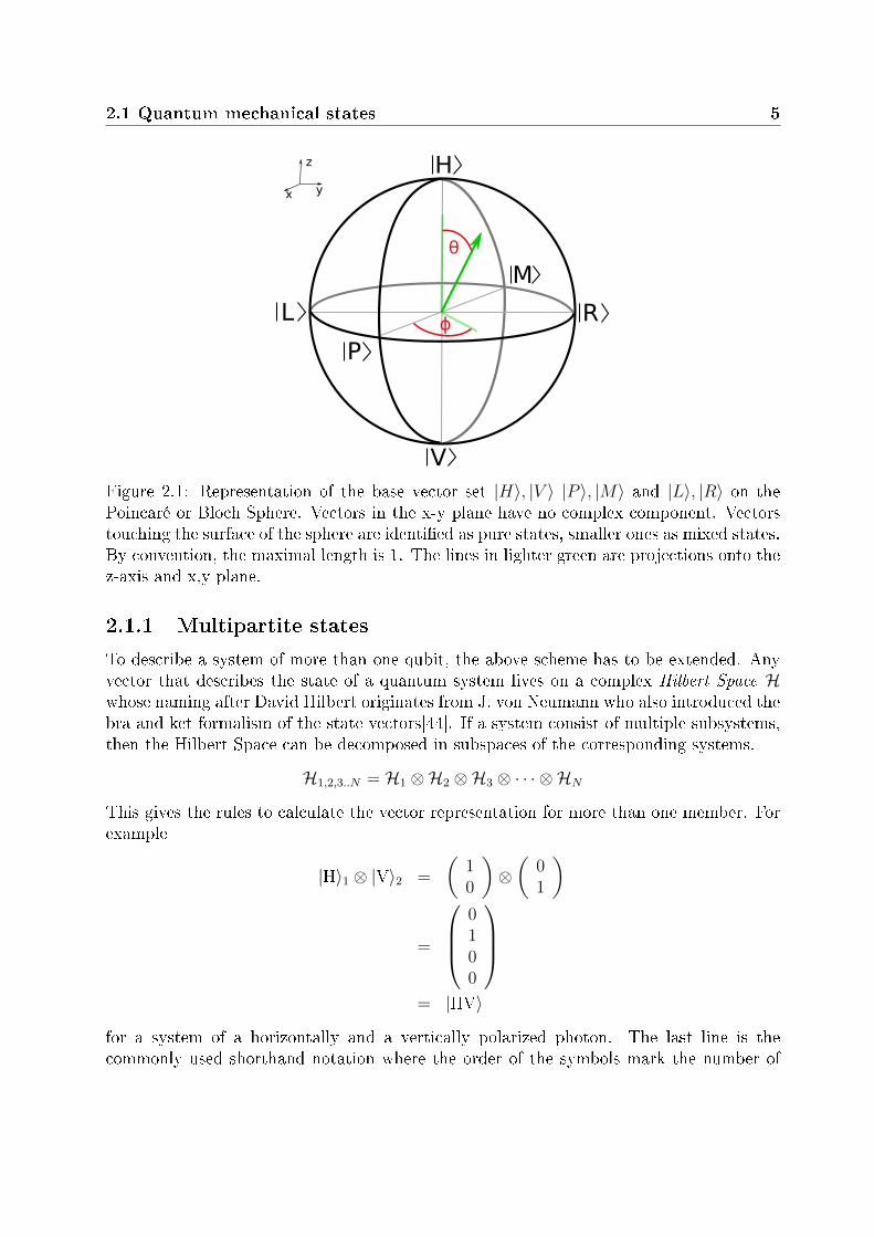
The convenient way to visualize a state of a single photon is through a vector on the BlochSphere (see �gure 2.1) or Poincaré Sphere with the polarization states as the orthogonalaxes. Originally this representation was developed by Henri Poincaré around 1892 todescribe polarization states of light and adapted by Felix Bloch in 1964[1] to polarizationstates of 2 level systems. E�ects of retarded (waveplates) and operations on the qubits arevisible as paths of the state vector on the surface. This pictorial power makes the spherea convenient tool of visualization.

Writing the polarization states as vectors, the projection operator of a state |ψ〉 isde�ned as P = |ψ〉〈ψ|. If this construct is acting onto another state |a〉

P|a〉 = |ψ〉〈ψ|a〉

the projection of |a〉 onto |ψ〉 in the direction |ψ〉 is calculated, where 〈ψ|a〉 is the scalarproduct of the 2 vectors. This behaviour gives raise to the naming in analogy to 3d vectors.For example |H〉〈H|ψ〉 corresponds to the projection of the green vector on |H〉, that is itscomponent along the positive z-direction. Two things are important to note:

� The above operation allows the extraction of components along e.g. an orthogonalbase set and likewise to determine its base vectors in this set. However the state ofthe qubit is changed, so it is not possible to use �the same� again, moreover it has tobe prepared in the same starting state again, or another one from the same source,in the same state must be used.

� In �gure 2.1, |H〉 is identi�ed with the positive, |V〉 with the negative z-direction.To anticipate chapter 2.2, a projection on either one of the previous vectors will becalled �measuring along the z-direction�. Likewise the other polarization types areidenti�ed with the generic x and y-direction.

Before turning to the full framework of measurements on qubits, the description of systemswith more members reviewed.

2.1 Quantum mechanical states 5

H

V

L R

P

M

x y

z

θ

ϕ

Figure 2.1: Representation of the base vector set |H〉, |V 〉 |P 〉, |M〉 and |L〉, |R〉 on thePoincaré or Bloch Sphere. Vectors in the x-y plane have no complex component. Vectorstouching the surface of the sphere are identi�ed as pure states, smaller ones as mixed states.By convention, the maximal length is 1. The lines in lighter green are projections onto thez-axis and x,y plane.

2.1.1 Multipartite states

To describe a system of more than one qubit, the above scheme has to be extended. Anyvector that describes the state of a quantum system lives on a complex Hilbert Space Hwhose naming after David Hilbert originates from J. von Neumann who also introduced thebra and ket formalism of the state vectors[44]. If a system consist of multiple subsystems,then the Hilbert Space can be decomposed in subspaces of the corresponding systems.

H1,2,3..N = H1 ⊗H2 ⊗H3 ⊗ · · · ⊗ HN

This gives the rules to calculate the vector representation for more than one member. Forexample

|H〉1 ⊗ |V〉2 =

(10

)⊗(

01

)

=

0100

= |HV〉

for a system of a horizontally and a vertically polarized photon. The last line is thecommonly used shorthand notation where the order of the symbols mark the number of

6 2. State description in quantum mechanics

the qubit so qubit 1 is said to be horizontally, qubit 2 vertically polarized. This space savingnotation is kept during this work. Generally for 2 systems with the basis decomposition|ψ〉 =

∑j

aj|ej〉 and |φ〉 =∑k

bk|fk〉 any product state can be written

|Ψ〉 =∑j

aj|ej〉 ⊗

(∑k

bk|fk〉

)=

∑j,k

cj,k|ej〉 ⊗ |fk〉

where the elements cj,k = aj · bk form a tensor. Another way to see this value is as a vectorwith the dimension of subsystem 1 where each element is again a vector with dimension ofsubsystem 2. The above way of writing a quantum state is called Schmidt Decomposition,named after Erhard Schmidt. The number of cj,k is called the Schmidt Rang. Not allquantum states have high ranks as the above formula might suggest. A special group,named entangled states, has rang 1.

2.1.2 Entanglement

As soon as a qubit state is a superposition of di�erent states, the claim that the HilbertSpace of a system can be decomposed in the subspaces of the subsystems does not holdany more. For example

|a〉 =1√2

(|HV〉+ |VH〉)

cannot be split in a state for each qubit. The 2 qubits are then called entangled [14]. Thegeneral de�nition reads[17]

A pure state |ψ〉 is called a product state or separable, if there are 2 states |φA〉and |φB〉 such that

|ψ〉 = |φA〉 ⊗ |φB〉

If this is not the case, |ψ〉 is called entangled.

The above state is a version of the famous EPR-Bohm-source state, where an atom changingfrom the excited into the unexcited state emits 2 photons of orthogonal polarization inopposing directions. Measuring horizontal polarization in the �rst direction it is clear thatthe other photon must be vertically polarized or vice versa. The correlation between statesis the essence of entanglement and cannot be described in mixtures.

2.1.3 Density matrices

The density operator or density matrix of a state |ψ〉is de�ned as ρ = |ψ〉〈ψ| and formallythe projector onto this state. What is known as the density matrix formalism [44] can

2.1 Quantum mechanical states 7

describe mixture of di�erent states. In quantum mechanics, the di�erence between super-position and mixture is crucial. Superpositions of states e.g. |H〉+ |V〉 form again a state(in this case |P〉) but a source can produce a certain number of |H〉, |V〉 and |P〉 photonsthat must be described by their proper polarization. The state of the complete system isdescribed as a (statistical) mixture of all contained states

ρ =∑i

pi|ai〉〈ai|

with∑i

pi = 1. Given that only a single pi is nonzero the state is said to be a pure state

and ρ2 = ρ holds. In this case the expression reduces to the above projector on the onlycontained state.

This also illustrates that the density matrix describes a quantum mechanical stateproduced by a source or setup in total. Extracting this operator is equivalent to having fullinformation on the state. However there are some requirements for the matrix to describea physical state. For example calculations that lead to expected outcome probabilitiesof more than 100% are not considered physical and therefore the matrix leading to suchresults cannot describe a system that can possibly exist. Such e�ects are excluded if thematrix obeys:

Hermiticity: The density operator is a hermitian operator

ρ = ρ†

This means that the hermitian conjugate3 or adjoint of the operator is again theoperator

Proof: (ρ)† =

(∑i

pi|ψi〉〈ψi|)†

=∑i

pi (|ψ〉〈ψ|)† =∑i

pi|ψi〉〈ψi| = ρ

Trace unity: The trace of any density operator is 1

Tr (ρ) = 1

Proof: Tr (ρ) =∑i,j

pj〈ψi|ψj〉〈ψj|ψi〉 =∑j

pj = 1

This can be understood as normalization of probability. The diagonal elements of adensity matrix represent the probability to measure the system in the state of thebase vector of the corresponding row and column. The space of the complete operatoris spanned by all base vectors, so the sum over the probabilities of all these must beunity.

3which is equivalent to transposing the matrix and taking the complex conjugate

8 2. State description in quantum mechanics

Positivity: The operator ρ is a positive operator

〈ψ|ρ|ψ〉 ≥ 0 ∀|ψ〉

Proof: 〈φ|ρ|φ〉 =∑i

pi〈φ|ψi〉〈ψi|φ〉 =∑i

pi |〈φ|ψi〉|2 ≥ 0

This is again a consequence of the probability interpretation. There are no negativeprobabilities.

2.1.3.1 Structure of a density matrix

Density operators of N qubit systems are 2N times 2N complex tensors. Values in the ma-trix depend on the basis vectors chosen. Standard bases are the bra end kets of horizontaland vertical polarization, in case of more than 1 member all permutations of them (seefollowing example 2.1). They can be generated by counting in binary numbers from 0 to2N −1 and identifying |H〉 with 0 and |V〉 with 14. In a 2 qubit example, the di�erent rowsand columns of the density matrix correspond to:

ρ =

〈HH| 〈HV| 〈VH| 〈VV|

|HH〉 ρ11 ρ12 · · ·|HV〉 ρ21 ρ22

|VH〉 .... . .

|VV〉 ...

(2.1)

Entries on the diagonal re�ect the probability for the system to be in the state of therow, respectively the column base vector. For |HH〉 this would be ρ11 = 〈HH|ρ|HH〉. O�-diagonal elements show correlations between those state. For example an entry in the�rst row and last column, 〈HH|ρ|VV〉, shows that |HH〉 and |VV〉 are present in a certainratio. An example would be the the state |ψ〉 = 1√

2(|HH〉+ |VV〉). The density operator

is calculated as

|ψ〉 =1√2

(|H〉 ⊗ |H〉+ |V〉 ⊗ |V〉) =1√2

1000

+

0001

=

1√2

1001

⇓

ρ = |ψ〉〈ψ| =1

2

1 0 0 10 0 0 00 0 0 01 0 0 1

4For example 42 corresponds to 101010 which gives |HVHVHV〉

2.1 Quantum mechanical states 9

Elements show that with equal probability either |HH〉 or |VV〉 will be measured and the

state to be a superposition. A mixture of the same states would lead to ρ = 12

1 0 0 00 0 0 00 0 0 00 0 0 1

missing the o�-diagonal elements.

2.1.3.2 Entanglement between systems

Not only single qubits but complete systems can be entangled, so the de�nition for entan-glement can be extended to density operators[45].

A state described by ρ is a product state, if two states ρA and ρB exist, suchthat

ρ = ρA ⊗ ρB

The state is separable if

ρ =∑i

pi (ρA)i ⊗ (ρB)i

with complex parameters pi. Otherwise the state is entangled.

It might seem that entanglement is solely of academic interest, because most experimentsuse well isolated systems. There are experiments that demonstrate entanglement in macro-scopic systems[23] but the e�ect is small and short-lived. However it can be used to pushthe so called �classical limits�. An example would be the Rayleigh di�raction limit[4] whichstates that a structures smaller than half the illuminating wavelength, cannot be resolvedand likewise exposed to light. Entangled photons allow the engineering of even smallerstructures[5] or increased accuracy in interferometers[27].

2.1.4 Measures

Having reconstructed a density matrix from measurements, one could ask how good thestate was prepared in comparison to the expected version or if it is a pure state. There areseveral measures for this

Purity Gives a measure if the density operator describes a pure state or a mixed one.

P (ρ) = Tr (ρ · ρ)

By de�nition of the idempotency of pure states and the constraint of trace unity it isclear that a pure state will have trace 1. A complete mixture will result in a value of1dwhere d are dimensions of ρ. Calculating the purity will show whether a mixture

has been observed or not.

10 2. State description in quantum mechanics

Fidelity Is a distance measure between 2 states and commonly used to characterizes thequality of a produced state. For this the measured state is compared to the expectedone. The �delity between 2 states ρ and φ is calculated as

F (ρ, φ) = Tr

(√√ρφ√ρ

)and is part of the Bures Distance[8] that is the �nite version of the original Buresmetric. Because ρ2 = ρ holds for pure states , the expression reduces to

F (ρ, φ) = Tr (ρ φ) = 〈φ|ρ|φ〉

which is the expectation value of one state with respect to the other. Accordinglythe �delity is 1 if the density operators describe the same state. This is the standardtool when density matrices, recovered from data are compared to expected states.

Another distance measure is the

Trace distance also called the Kolmogorov Distance or trace norm distance[16]

δ (ρ, φ) =1

2Tr (ρ− φ)

The original distance measure was developed for probability distributions in gen-eral, but as density operators describe the probability distribution for a state, theexpression can be cast into this form for such operators.

There exist a lot more types of measures but for a general inspection of the results, theabove su�ce.

2.2 Measurements

In quantum mechanics, observables are represented by hermitian operators. A state beingin a superposition |ψ〉 =

∑i

ci|ai〉 will be forced into an eigenstate (any |ak〉) of the operator

when the corresponding observable is measured. This is also why measurements are oftencalled projective measurements, as they project the original state onto another one.

ρa|ψ〉 = |a〉〈a|ψ〉 = c|a〉

where c = 〈a|ψ〉 is the projection of |ψ〉 along |a〉.The expectation value of an observable O with respect to a state |a〉 is de�ned as

〈a|O|a〉 =∑i

〈a|i〉〈i|O|a〉

=∑i

〈i|O|a〉〈a|i〉

=∑i

〈i|O ρa|i〉

= Tr (O ρa) (2.2)

2.2 Measurements 11

This expression already occurred in the de�nition of the �delity for pure states.For photonic qubits a generic observable reads

O (θ, φ) = cos (θ)σz + cos (φ) sin (θ)σx + sin (φ) cos (θ)σy (2.3)

where the angles θ and φ identify an axis through the origin of the Bloch Sphere. ThePauli Spin Matrices5

σx =

(1 00 −1

)σy =

(0 −ii 0

)σz =

(0 11 0

)form the orthogonal basis set that spans the space. The polarization states of the photonicqubit can be identi�ed with the eigenstates of the Pauli Matrices

σx|P/M〉 = ±|P/M〉σy|R/L〉 = ±|R/L〉σz|H/V〉 = ±|H/V〉

This justi�es the previous geometric interpretation of an axis through the sphere and iden-ti�es σx,y,z as the 3 generic and orthogonal directions x,y and z. Measuring the expectationvalue of, for instance σy, is equivalent to project the state onto the y-axis and the processwill just be called �measuring along the y-axis�.

In an experiment, one does not aim to project along an axis but merely on a speci�cstate. A handy expression for the projector on a polarization state in terms of its PauliMatrix is6

Pi,± =1

2(1± σi) (2.4)

where the sign is equal to the one of the eigenvalue one wants to project onto. Thisexpression is only valid for systems of 2 members and used to calculate the probability tomeasure the qubit in a certain polarization state via Tr (Pi,±ρ).

Observables for systems with more than one qubit, can be calculated in a similar wayusing the tensor product. Acting only on qubit 1 in a 2 qubit system, the operator of theobservable is written as O1 ⊗ 1 or likewise 1 ⊗ O2 for qubit 2. The combined operatorreads O1 ⊗ O2. Also e�ects of wave plates are described by operators (see chapter 2.3 forexpressions), consecutive operations by products of the operators. Combined with tensorproducts, operators act only on their subspace and so do successive operations

(A1 ⊗ A2) · (B1 ⊗B2) = (A1 ·B1)⊗ (A2 ·B2)

5There is a fourth Pauli Matrix, the unit matrix σ0 =

(1 00 1

)that is left out here, but is needed int

he following formulas to reconstruct the density matrix. Often instead of {x, y, z} the labels {1, 2, 3} areused

6Any pauli matrix can be decomposed as σi = |+〉〈+|−|−〉〈−| with |+〉 the positive eigenvector and |−〉the negative eigenvector. Also 1 = |+〉〈+|+ |−〉〈−| and therefore 1 = |+〉〈+|+ |+〉〈+|−σi = 2|+〉〈+|−σi→ |+〉〈+| = 1

2 (1+ σi) and analogue for |−〉〈−|

12 2. State description in quantum mechanics

In general, multiplication of operators is not commutative, but associative

A (B · C) = (A ·B)C 6= (B · A)C

Their commutation behaviour is described by the commutator, de�ned as [A,B] = AB −BA. If it is zero, they commute, otherwise they commute as stated. For example the paulimatrices obey

[σi, σj] = 2 i εijkσk

with the Levi-Civita symbol εijk. This would lead to σxσy = σyσx − 2iσz.

This relation re�ects the surprising fact that certain measurements in quantum me-chanics are order sensitive. The outcome will change depending on the order they areperformed, something not known from macroscopic systems. The previous section showsthat this is a result of the state being projected onto an eigenstate of the observable andtherefore being subject to change.

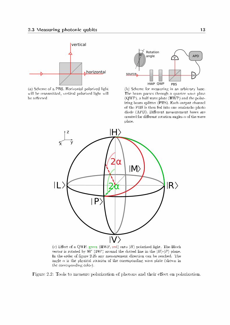
2.3 Measuring photonic qubits

To analyze the polarization of a photonic qubit, a polarizing beam splitter (PBS), a quarterwave plate (QWP or λ

4-plate), a half wave plate (HWP or λ

2-plate) and a single photon

counting module (here Avalanche Photo Diodes) are arranged to a polarization analysisblock (�g. 2.2b).

The PBS will split an unpolarized light beam into its horizontal and vertical component(see �gure 2.2a) or likewise distribute photons according to their projection onto the |H〉,|V〉(or z) axis (base). For example P polarized photons will be detected with equal probabilityin either the horizontal or vertical output channels. H polarized ones on the other side with100% (for an ideal PBS) in the horizontal one. Because the probability depends on theprojection onto the z base, a PBS will experimentally implement the operation Tr (σzρ).If one is interested in the probabilities for a detection in either output channel, one has tocalculate Tr (Pz,+ρ) for |H〉 or Tr (Pz,−ρ) for |V〉. Detection in the APD absorbs the photon,so the source used needs to produce the same state with high reliability because consecutivemeasurements are necessary to collect enough data. To realize arbitrary measurementdirections (see eq. 2.3), the combination of a HWP, QWP and a PBS is necessary.

A HWP rotates the state vector by 180° around an axis in the |H〉|V〉-|P〉|M〉 plane,given by 2 times the physical rotation (α) (in the plane perpendicular to the incident beam)of the crystal itself. The 0° position is de�ned as the position where horizontal polarizedlight stays horizontal and vertical polarized stays vertical or in other words the rotationaxis concurs with the z-axis in the Bloch Sphere. The operator for a HWP reads

HWP (α) =

(cos (2α) sin (2α)sin (2α) − cos (2α)

)= sin (2α) σ̂x + cos (2α) σ̂z (2.5)

2.3 Measuring photonic qubits 13

horizontal

vertical

(a) Scheme of a PBS. Horizontal polarized lightwill be transmitted, vertical polarized light willbe re�ected

source

QWPHWP PBS

APD

H

Vα

Rotationangle

(b) Scheme for measuring in an arbitrary base.The beam passes through a quarter wave plate(QWP), a half wave plate (HWP) and the polar-izing beam splitter (PBS). Each output channelof the PBS is then fed into one avalanche photodiode (APD). Di�erent measurement bases arecreated for di�erent rotation angles α of the waveplate.

H

V

L R

P

M2α

x y

z

2α

(c) E�ect of a QWP, green (HWP, red) onto |H〉 polarized light. The Blochvector is rotated by 90° (180°) around the dotted line in the |H〉-|P 〉 plane.In the order of �gure 2.2b any measurement direction can be reached. Theangle α is the physical rotation of the corresponding wave plate (shown inthe corresponding color).

Figure 2.2: Tools to measure polarization of photons and their e�ect on polarization.

14 2. State description in quantum mechanics

The e�ect on a vertically polarized photon propagating through a HWP rotated by 45°is that it will become horizontally polarized or likewise plus polarized when incident on a22.5° rotated HWP (red line in �gure 2.2c).

A QWP rotates the state vector by 45° around an axis with the same de�nition as inthe HWPs' case. The operator reads

QWP (α) =

(cos2 (α)− i sin2 (α) (1 + i) cos (α) sin (α)

(1 + i) cos (α) sin (α) −i cos2 (α) + sin2 (α)

)=

1

2[(1− i) 1 + 2 (1− i) cos (α) sin (α) σ̂x + (1 + i) cos (2α) σ̂z] (2.6)

and will rotate a right polarized photon into horizontal polarization for a wave plate rota-tion of 45° (green line in �gure 2.2c).

When measuring in arbitrary bases, the idea is to rotate the positive eigenvector (|R〉 or|+〉) onto |H〉 and the negative one (|L〉 or |−〉) onto |V〉. This way, the PBS will e�ectivelyproject onto the positive or negative eigenvector of the desired direction. The angles of thewave plates for the 3 standard directions are

measurement direction HWP QWP

X (σx) 22.5° 0°

Y (σy) 0° 45°

Z (σz) 0° 0°

To measure along an arbitrary direction, the relation

σ̂z = [QWP (α2) · HWP (α1)] σ̂ (θ, φ) [QWP (α2)HWP (α1)]† (2.7)

has to be solved. The solutions are ambiguous but will result in the correct outgoingpolarization.

A complete setup for the analysis of a single photonic qubit state is shown in �gure2.2b. This scheme is however not the only possible one. Another implementation wouldexchange the PBS by a polarizer[22]. Downside of this approach is the loss in count rate,because photons that are projected onto the orthogonal state for which the polarizer istransmittive, are lost. In the later chapters it will become clear that high count rates arecrucial, thus the version with a PBS is chosen.

3 Quantum State Tomography

Tomography originates from the Greek word �tomos� that means �part� and �graphein�what can be translated as �to write�. From a set of images that contain reduced informa-tion about the object, the complete object is reconstructed. For example the 3D contentof a picture can be extracted from several 2D pictures taken from di�erent directions. Thisis also the basic idea for quantum state tomography where the state is projected on a setof di�erent bases, called the tomographic set. Instead of extracting just a single propertyvia so called witnesses e.g. entanglement[17], state tomography aims to extract all possi-ble information about the state that are contained in the density operator. Section 2.1.3motivated the structure of the density matrix and showed that knowledge of this operatorsu�ces to describe a system in total. Behaviour under certain operations and measurementoutcomes can be calculated. This means that from the measurement of selected propertiesof a system, other can be inferred and this is what tomography is about. In the follow-ing sections, state tomography of single qubits will be introduced and later on extendedarbitrary qubit numbers. Because the amount of data that need to be measured scalesexponentially in the number of qubits, a di�erent and more e�ective but more restrictivetomography method is presented. In this new scheme the data increase can be reduced toa quadratic scaling of the qubit number.

3.1 Tomography of a single qubit

The state of a qubit, represented by a vector in the Bloch Sphere, is �xed by 3 parameters.Either 2 angles and the length of the vector, like in spherical coordinates, or 3 valuesthat are the projections on a set of 3 orthogonal axes, like the standard x,y and z-axisconvention. Previously it was shown that measuring the expectation values of σx, σy andσz is the equivalent to a projection on the generic x,y and z directions.

Descriptions of polarized light have a longer history than states of qubits and weredeveloped for light beams rather than individual photons. Nevertheless, the same schemecan be used for qubits. The commonly used parameters were introduced by G. G. Stokesin 1852 and are therefore called the Stokes Parameter. They are de�ned in terms ofelectric �eld amplitudes for di�erent types of polarization[4] and originally motivated the

16 3. Quantum State Tomography

H

V

L R

P

Ms3

2s

1sx y

z

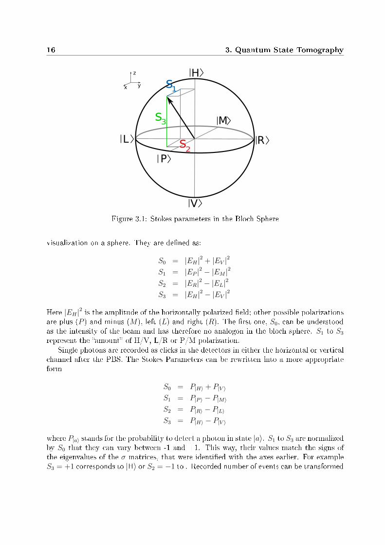
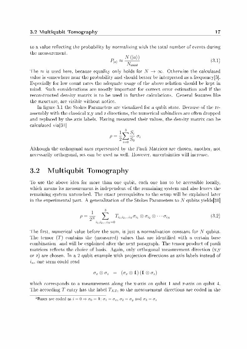
Figure 3.1: Stokes parameters in the Bloch Sphere

visualization on a sphere. They are de�ned as:

S0 = |EH |2 + |EV |2

S1 = |EP |2 − |EM |2

S2 = |ER|2 − |EL|2

S3 = |EH |2 − |EV |2

Here |EH |2 is the amplitude of the horizontally polarized �eld; other possible polarizationsare plus (P ) and minus (M), left (L) and right (R). The �rst one, S0, can be understoodas the intensity of the beam and has therefore no analogon in the bloch sphere. S1 to S3

represent the �amount� of H/V, L/R or P/M polarization.Single photons are recorded as clicks in the detectors in either the horizontal or vertical

channel after the PBS. The Stokes Parameters can be rewritten into a more appropriateform

S0 = P|H〉 + P|V 〉

S1 = P|P 〉 − P|M〉S2 = P|R〉 − P|L〉S3 = P|H〉 − P|V 〉

where P|a〉 stands for the probability to detect a photon in state |a〉. S1 to S3 are normalizedby S0 that they can vary between -1 and +1. This way, their values match the signs ofthe eigenvalues of the σ matrices, that were identi�ed with the axes earlier. For exampleS3 = +1 corresponds to |H〉 or S2 = −1 to . Recorded number of events can be transformed

3.2 Multiqubit Tomography 17

to a value re�ecting the probability by normalizing with the total number of events duringthe measurement.

P|a〉 ≈N (|a〉)Ntotal

(3.1)

The ≈ is used here, because equality only holds for N → ∞. Otherwise the calculatedvalue is somewhere near the probability and should better be interpreted as a frequency[3].Especially for low count rates the adequate usage of the above relation should be kept inmind. Such considerations are mostly important for correct error estimation and if thereconstructed density matrix is to be used in further calculations. General features likethe structure, are visible without notice.

In �gure 3.1 the Stokes Parameters are visualized for a qubit state. Because of the re-assembly with the classical x,y and z directions, the numerical subindices are often droppedand replaced by the axis labels. Having measured their values, the density matrix can becalculated via[31]

ρ =1

2

3∑i=0

SiS0

σi

Although the orthogonal axes represented by the Pauli Matrices are chosen, another, notnecessarily orthogonal, set can be used as well. However, uncertainties will increase.

3.2 Multiqubit Tomography

To use the above idea for more than one qubit, each one has to be accessible locally,which means its measurement is independent of the remaining system and also leaves theremaining system untouched. The exact prerequisites to the setup will be explained laterin the experimental part. A generalization of the Stokes Parameters to N qubits yields[31]

ρ =1

2N

3∑i1,i2,...iN=0

Ti1,i2,...iNσi1 ⊗ σi2 ⊗ · · ·σiN (3.2)

The �rst, numerical value before the sum, is just a normalization constant for N qubits.The tensor (T ) contains the (measured) values that are identi�ed with a certain basecombination1 and will be explained after the next paragraph. The tensor product of paulimatrices re�ects the choice of basis. Again, only orthogonal measurement direction (x,yor z) are chosen. In a 2 qubit example with projection directions as axis labels instead ofin, one term could read

σx ⊗ σz = (σx ⊗ 1) (1⊗ σz)

which corresponds to a measurement along the x-axis on qubit 1 and z-axis on qubit 4.The according T entry has the label TXZ , so the measurement directions are coded in the

1Bases are coded as i = 0⇒ σ0 = 1; σ1 = σx, σ2 = σy and σ3 = σz

18 3. Quantum State Tomography

order and label of the subindex. When for a single qubit the orthogonal bases, including the(normalized) intensity parameter, had to be measured, for multiple qubits all combinationsfor all members are needed. For example the element TX1 with the corresponding operator

σx ⊗ 1 or T1Y with 1⊗ σy. Normalization is done with respect to T11···1!

= 1, so there arein general 2N × 2N − 1 entries that have to be determined through measurements.

The use of the PBS allows a so called overcomplete measurement. For this, it is instruc-tive to have a look at the T entries and how they relate to the one qubit Stokes Parameters.In a small 2 qubit example, one could naively write

TZY = TZ ⊗ TY= S3 ⊗ S2

=(P|H〉 − P|V 〉

)⊗(P|R〉 − P|L〉

)= P|HR〉 − P|HL〉 − P|V R〉 + P|V L〉 (3.3)

where the tensor product is used here to discriminate between measurements on qubit 1and qubit 2 and should not be regarded as a mathematical operation. The last line showsthat the needed values are for example the probability to measure qubit 1 in state |H〉 andsimultaneously qubit 2 in state |R〉 (P|HR〉) and the other permutations for the used bases.If a �1 measurement� is involved, the expression reads

T1Y = T1 ⊗ TY= S0 ⊗ S2

=(P|H〉 + P|V 〉

)⊗(P|R〉 − P|L〉

)(3.4)

= P|HR〉 − P|HL〉 + P|V R〉 − P|V L〉

so the same values as for the previous expression can be used. To make use of the PBS,events in all channels have not only to be recorded, but also concurrent events. Theanalysis of a single qubit requires the measurement of H and V events. Already for 2qubits, simultaneous events in channel H on qubit 1 and channel V on qubit 2 (and allother permutations) are possible. Although one settings (like TZX or T1Y ) is said to be onemeasurement, 2N values are recorded: the concurrent detections of photons in di�erentPBS output con�gurations (like HH, HV, VH and VV). A scheme of a 2 qubit example isshown in �gure 5.3, illustrating possible combinations. Because a large number of recordedvalues is reduced to fewer T entries, this scheme is called overcomplete.

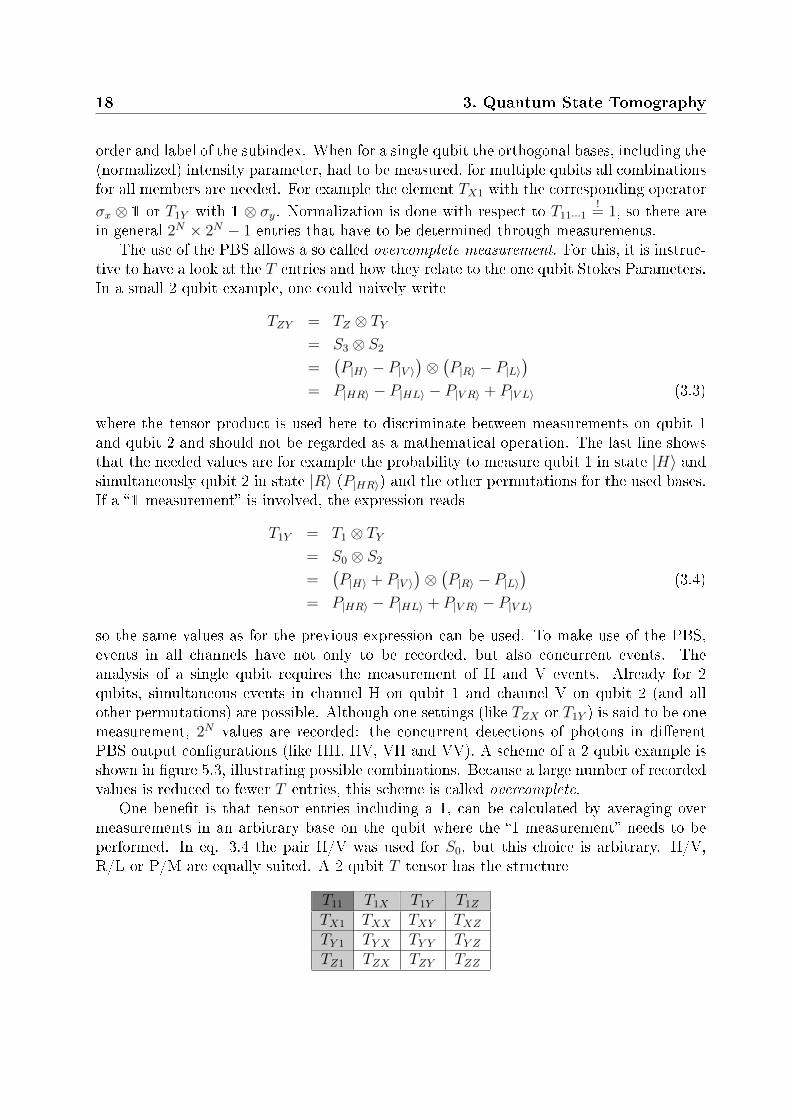
One bene�t is that tensor entries including a 1, can be calculated by averaging overmeasurements in an arbitrary base on the qubit where the �1 measurement� needs to beperformed. In eq. 3.4 the pair H/V was used for S0, but this choice is arbitrary. H/V,R/L or P/M are equally suited. A 2 qubit T tensor has the structure

T11 T1X T1Y T1ZTX1 TXX TXY TXZTY 1 TY X TY Y TY ZTZ1 TZX TZY TZZ

3.3 Permutationally Invariant Quantum State Tomography 19

with the T11 = 1 normalized entry marked in dark gray and the ones that are calculatedfrom values in the corresponding row or column in lighter gray. Instead of 2N × 2N − 1 =4N − 1, only 3N − 1 unique settings (combinations of measurement bases) need to bedetermined, if correlations in the outputs of the PBS are recorded.

There are no restrictions to the state analyzed via this scheme, so it is called Full To-mography. A major problem of multiqubit states produced by most sources and is the lowcount rate, if one seeks states with large numbers of genuine entangled qubits. Becausecorrelation information are important to detect entanglement, the number of terms in thestandard tomography scheme increases exponentially in the number of qubits (3N − 1).For reasonable statistics, time needed for the measurement increases with the same rate.This combination of exponential increase in time and exponential decrease in brightnessimmediately leads to problems. For the described experiment, the analysis of the 6 qubitsymmetric Dicke State, full tomography is already out of reach. Good statistics wouldrequire a month of 24h a day, 7 days a week non-stop measurement, what is not possiblewith the used setup. Using symmetries in the states allows a reduction to 24h of measure-ment time with the same precision. The vast di�erence in the necessary time re�ects thereduction of individual measurement settings from O

(3N)to O (N2).

3.3 Permutationally Invariant Quantum State Tomog-

raphy

Most states of interest show certain symmetries. They can be chosen on purpose, becausethe state is more tolerant against loss of entanglement if individual photons are lost, orthe process in the source impresses its symmetry. The following is designed for permu-tationally invariant (PI) states. Such states are invariant under exchange of arbitraryqubits. A simple example would be the bell state 1√

2(|HV〉+ |VH〉); summation ensures

that exchange of qubit 1 and 2 will just change the order, with no e�ect for the overallstate. |Ψ−〉 = 1√

2(|HV〉 − |VH〉) on the other hand does not obey this symmetry because

the phase factors in front of the polarization states are not recovered.The formal de�nition of PI symmetry is[40]

ρPI =1

N !

∑k

ΠkρΠk

where Πk are the permutations of all qubits. Any density operator has a part that ful�llsthe above equation, but the state it describes does not necessarily lie in this subspace. Withthis in mind, one can state that any density operator has a part that is permutationallyinvariant, and a part that is not:

ρ = ρnonPI + ρPI

The downside of PI tomography is, that the ρnonPI part will not be visible. Fortunatelywhite noise, which is of most interest when characterizing an experiment in terms of per-formance, is PI symmetric and will therefore be visible.

20 3. Quantum State Tomography

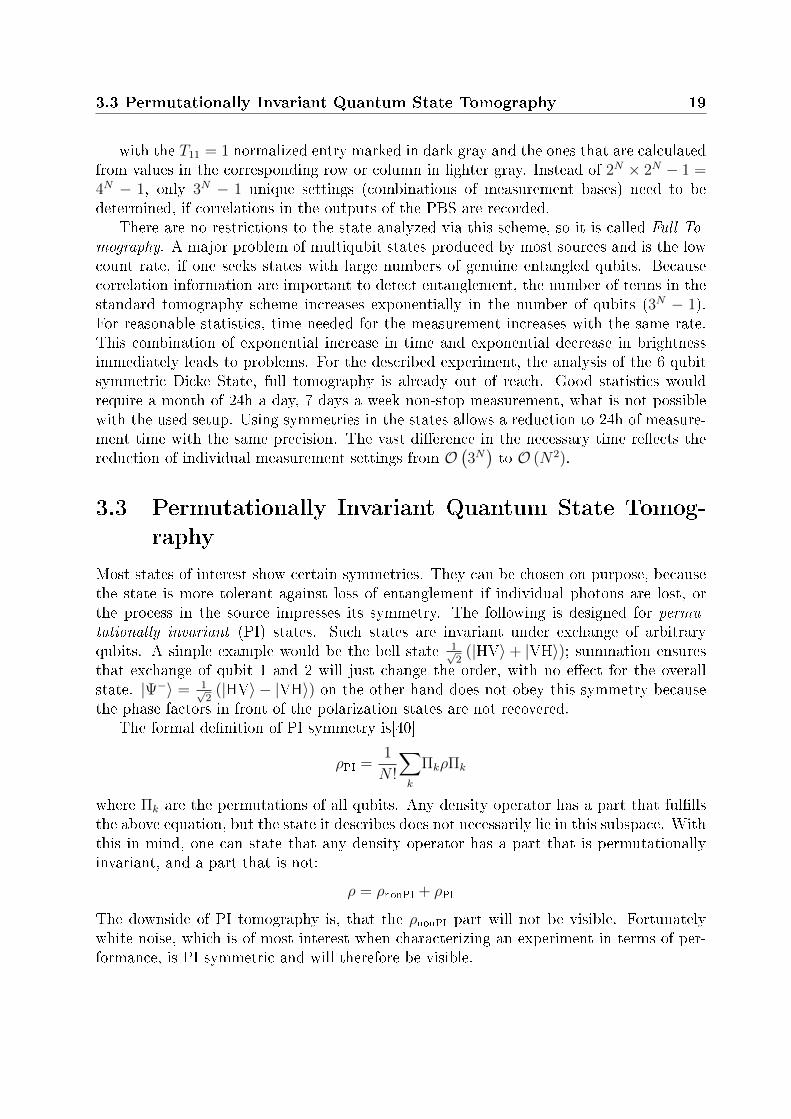
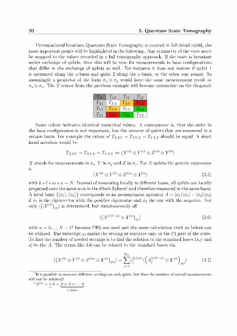
Permutational Invariant Quantum State Tomography is covered in full detail in[40], themost important points will be highlighted in the following. Any symmetry of the state mustbe mapped to the values recorded in a full tomography approach. If the state is invariantunder exchange of qubits, then this will be true for measurements in base con�gurationsthat di�er in the exchange of qubits as well. For instance it does not matter if qubit 1is measured along the x-basis and qubit 2 along the y-basis, or the other way round. Soassumingly a projector of the form σx ⊗ σy would have the same measurement result asσy ⊗ σx. The T tensor from the previous example will become symmetric on the diagonal:

T11 T1X T1Y T1ZTX1 TXX TXY TXZTY 1 TY X TY Y TY ZTZ1 TZX TZY TZZ

Same colour indicates identical numerical values. A consequence is, that the order inthe base con�guration is not important, but the amount of qubits that are measured in acertain basis. For example the values of TXXY = TXYX = TY XX should be equal. A shorthand notation would be

TXXY = TXYX = TY XX ⇔ 〈X⊗2 ⊗ Y ⊗1 ⊗ Z⊗0 ⊗ 1⊗0〉

X stands for measurements in σx, Y in σy and Z in σz. For N qubits the generic expressionis

〈X⊗k ⊗ Y ⊗l ⊗ Z⊗m ⊗ 1⊗n〉 (3.5)

with k+l+m+n = N . Instead of measuring locally in di�erent bases, all qubits are locallyprojected onto the same axis in the Bloch Sphere2 and therefore measured in the same basis.A local basis {|φ1〉, |φ2〉} corresponds to an measurement operator A = |φ1〉〈φ1| − |φ2〉〈φ2|if φ1 is the eigenvector with the positive eigenvalue and φ2 the one with the negative. Notonly 〈

(A⊗N

)PI〉 is determined, but simultaneously all

〈(A⊗(N−n) ⊗ 1

⊗n)PI〉 (3.6)

with n = 0, ..., N − 13 because PBS are used and the same calculation trick as before canbe utilized. The subscript PI marks the setting as sensitive only to the PI part of the state.To �nd the number of needed settings is to �nd the relation to the standard bases (x,y andz) to the A. The terms like 3.6 can be related to the standard bases via

〈(X⊗k ⊗ Y ⊗l ⊗ Z⊗m ⊗ 1

⊗n)PI〉 =

DN∑j=1

c(k,l,m)j 〈

(A⊗(N−n)j ⊗ 1

⊗n)PI〉 (3.7)

2It is possible to measure di�erent settings on each qubit, but then the number of overall measurementswill not be minimal!

3A⊗n = ⊗nA = A⊗A⊗ · · ·A︸ ︷︷ ︸

n times

3.3 Permutationally Invariant Quantum State Tomography 21

DN then is the number of settings that are needed to calculate ρ, with a small detour overthe 3.5 terms. Its value is found by some combinatorial considerations, �nding the spacespanned by 3.5.

The most exact information about a vector is given in terms of an orthogonal base set.If projective measurements of a qubit are just performed onto the H/V,P/M plane, thereis no chance to determine a state correctly that has contributions in the R/L direction.Merely its projection onto the plane is measured. The result space then can be consideredto be of lower dimension than the source space. To determine DN , the dimension of thespace spanned by 3.5 needs to be found4, because eq. 3.7 states that the same space isspanned by DN directions of type 3.6.

Overall there are

DN−n =

(N − n+ 2N − n

)possibilities where k+ l+m+n = N holds and a previously unknown direction is covered.In other word the term describes the expectation value of a measurement direction thatis orthogonal to all previous ones. All terms of type 3.5 contribute one expectation value,because the state can be projected along each counted dimension. For n > 0 DN−ndecreases, so to map the full tomographic set to the new directions Aj, DN settings mustbe chosen. Otherwise less dimensions could be covered and not the full state but theprojection on a subspace is measured. The necessary number can then be calculated via

DN =

(N + 2N

)=

1

2

(N2 + 3N + 2

)(3.8)

From the afore shown decomposition the values of T for eq. 3.2 can be calculated. Whatis left now is to �nd a set of Aj and cj. The overall statistical uncertainty needs to beminimized, which is the sum of the variances of the Bloch vector

(Etotal)2 =∑

k+l+m+n=N

E2[(X⊗k ⊗ Y ⊗l ⊗ Z⊗m ⊗ 1

⊗n)] N !

k!l!m!n!

where the variance of a single element is

E2[(X⊗k ⊗ Y ⊗l ⊗ Z⊗m ⊗ 1

⊗n)] =

DN∑j=1

∣∣∣c(k,l,m)j

∣∣∣2 E2 [(A⊗(N−n)j ⊗ 1⊗n)PI

]︸ ︷︷ ︸

∗

The variance of expression * depends on the statistic of the experiment. For the followingphotonic setup, a Poissonian distribution can be assumed

E2[(A⊗(N−n)j ⊗ 1

⊗n)PI

]=

[∆(A⊗(N−n)j ⊗ 1

⊗N)PI

]2ρ0

λj − 1

4This is valid because these terms are known from full tomography to span the full result space

22 3. Quantum State Tomography

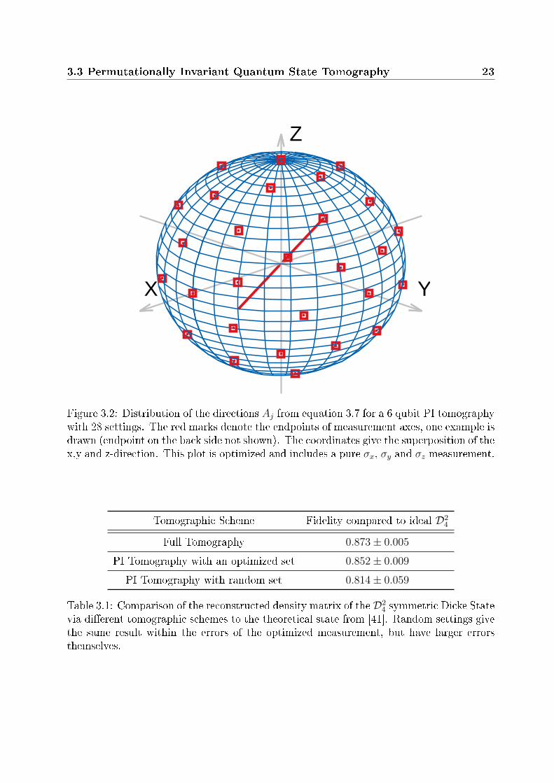
with the Poisson Parameter λj and (∆A)2ρ0 = 〈A2〉ρ0 − 〈A〉2ρ0 with respect to a state ρ0of the system that has to be guessed. In the best case information about the estimatedstate is known and plugged in here, otherwise a complete mixture can be used. This wouldcorrespond to no knowledge on the state at all. From these formulas an expression foroptimal cj for a set of given Aj can be cast. To minimize the uncertainties with respectto the Aj, an equal distribution on the Bloch Sphere should be chosen. Alternatively arandom set will work as well, but the errors will increase[40]. An example distributionis plotted in �gure 3.2 where each point on the surface of the Bloch Sphere marks theintersection of a measurement axes of the form A = x · σx + y · σy + z · σz. The continuousline is an example where 2 endpoints are connected. Because the same basis is measuredon all qubits, it can be visualized on the Bloch Sphere of a single qubit. Together with theset of cj's the state can be reconstructed. In the later performed 6 qubit tomography, thecj's form a tensor of dimension 28x83. The index j �xes the �rst dimension, the seconddepends on possible combinations of k+ l+m. There is a block of values for k+ l+m = N ,a block for k + l + m = N − 1, for k + l + m = N − 2 etc until k + l + m = 1 is reached.In Matlab, the following code will calculate this number.

dim = 0 ;for i=NQubits :−1:1

dim = dim + nchoosek ( i +2, i ) ;end

The above described blocks are iterated for �NQubits� qubits in the system and thenumber of possible distributions is summed up. The function nchoosek(n,k) calculates(nk

). In the case for NQubits=6, the result will be 83. This is also the number of

〈(X⊗k ⊗ Y ⊗l ⊗ Z⊗m ⊗ 1⊗n

)PI〉 type expectation values that are calculated and describe

unique correlations from which the density operator is calculated. Full tomography woulduse 3N (= 729 for 6 qubits) correlations and therefore more measured values contribute toindividual entries in the density matrix. This is quanti�ed in appendix B and shows thatindeed the average number of values for an entry is lowered by a factor 5.44 compared toFull Tomography.

Table 3.1 gives the results from[40] for a 4 qubit measurement and illustrates the be-haviour of PI tomography with an optimized and random set to a full tomographic mea-surement. Although the �delity is smaller for both PI schemes, the optimized versionachieves good results.

Overlap with with the symmetric subspace

Any tomography is performed to gain information about an previously unknown state butPI tomography requires the state to be PI symmetric. With the relation

P (6)s ≥

2

225

(J2x + J2

y + J2z

)− 1

90

(J4x + J4

y + J4z

)+

1

450

(J6x + J6

y + J6z

)(3.9)

3.3 Permutationally Invariant Quantum State Tomography 23

X Y

Z

Figure 3.2: Distribution of the directions Aj from equation 3.7 for a 6 qubit PI tomographywith 28 settings. The red marks denote the endpoints of measurement axes, one example isdrawn (endpoint on the back side not shown). The coordinates give the superposition of thex,y and z-direction. This plot is optimized and includes a pure σx, σy and σz measurement.

Tomographic Scheme Fidelity compared to ideal D24

Full Tomography 0.873± 0.005

PI Tomography with an optimized set 0.852± 0.009

PI Tomography with random set 0.814± 0.059

Table 3.1: Comparison of the reconstructed density matrix of the D24 symmetric Dicke State

via di�erent tomographic schemes to the theoretical state from [41]. Random settings givethe same result within the errors of the optimized measurement, but have larger errorsthemselves.

24 3. Quantum State Tomography

an estimation to the overlap with the symmetric subspace can be made. Jx = 12

∑k

Xk,

Jy = 12

∑k

Yk and Jz = 12

∑k

Zk and Xk are the σx operator on the kth qubit5. The space

is the one of the symmetric Dicke State[11], that will be introduced later. Values of theJi can be extracted from measurements along the X,Y and Z-direction on all qubits. Aderivation of the exact relation is done in appendix A.

To use this estimation, 3 measurement directions have to be �xed but fortunatelyPI Tomography gives some freedom in choosing the Aj in eq. 3.7. Finding a set ofmeasurement directions that includes X,Y and Z is then straightforward and the recordeddata can be used for the state reconstruction as well.

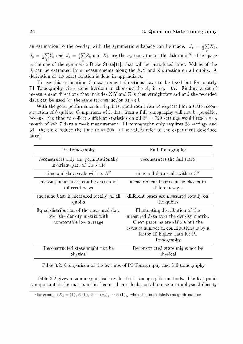
With the good performance for 4 qubits, good result can be expected for a state recon-struction of 6 qubits. Comparison with data from a full tomography will not be possible,because the time to collect su�cient statistics on all 36 = 729 settings would reach ≈ amonth of 24h 7 days a week measurement. PI tomography only requires 28 settings andwill therefore reduce the time to ≈ 20h. (The values refer to the experiment describedlater)

PI Tomography Full Tomography

reconstructs only the permutationallyinvariant part of the state

reconstructs the full state

time and data scale with ∝ N2 time and data scale with ∝ 3N

measurement bases can be chosen indi�erent ways

measurement bases can be chosen indi�erent ways

the same base is measured locally on allqubits

di�erent bases are measured locally onthe qubits

Equal distribution of the measured dataover the density matrix withcomparable low average

Fluctuating distribution of themeasured data over the density matrix.

Clear patterns are visible but theaverage number of contributions is by a

factor 10 higher than for PITomography

Reconstructed state might not bephysical

Reconstructed state might not bephysical

Table 3.2: Comparison of the features of PI Tomography and full tomography

Table 3.2 gives a summary of features for both tomographic methods. The last pointis important if the matrix is further used in calculations because an unphysical density

5for example Xk = (1)1 ⊗ (1)2 ⊗ · · · (σx)k · · · ⊗ (1)N when the index labels the qubit number

3.3 Permutationally Invariant Quantum State Tomography 25

matrix can lead to unreasonable result in some measures. Reconstructed stays for a directuse of formulae 3.2 and 3.7 with the recorded values and without taking any statistics intoaccount.

26 3. Quantum State Tomography

4 Maximum Likelihood Estimation

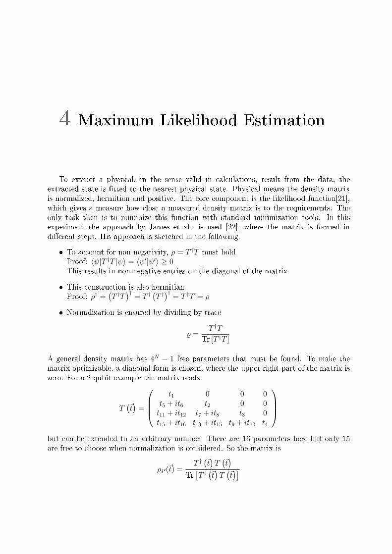
To extract a physical, in the sense valid in calculations, result from the data, theextracted state is �tted to the nearest physical state. Physical means the density matrixis normalized, hermitian and positive. The core component is the likelihood function[21],which gives a measure how close a measured density matrix is to the requirements. Theonly task then is to minimize this function with standard minimization tools. In thisexperiment the approach by James et al. is used [22], where the matrix is formed indi�erent steps. His approach is sketched in the following.

� To account for non negativity, ρ = T †T must holdProof: 〈ψ|T †T |ψ〉 = 〈ψ′|ψ′〉 ≥ 0This results in non-negative entries on the diagonal of the matrix.

� This construction is also hermitianProof: ρ† =

(T †T

)†= T †

(T †)†

= T †T = ρ

� Normalization is ensured by dividing by trace

% =T †T

Tr [T †T ]

A general density matrix has 4N − 1 free parameters that must be found. To make thematrix optimizable, a diagonal form is chosen, where the upper right part of the matrix iszero. For a 2 qubit example the matrix reads

T(~t)

=

t1 0 0 0

t5 + it6 t2 0 0t11 + it12 t7 + it8 t3 0t15 + it16 t13 + it15 t9 + it10 t4

but can be extended to an arbitrary number. There are 16 parameters here but only 15are free to choose when normalization is considered. So the matrix is

ρP (~t) =T †(~t)T(~t)

Tr[T †(~t)T(~t)]

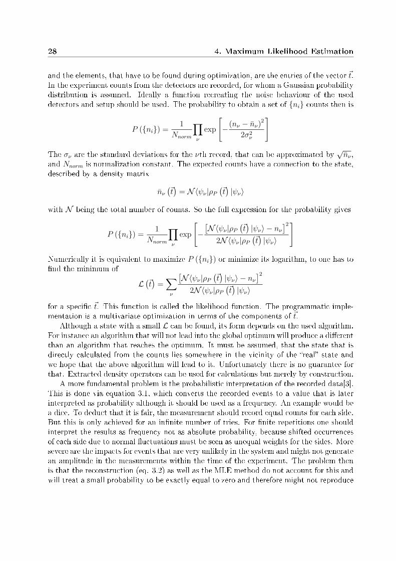
28 4. Maximum Likelihood Estimation

and the elements, that have to be found during optimization, are the entries of the vector ~t.In the experiment counts from the detectors are recorded, for whom a Gaussian probabilitydistribution is assumed. Ideally a function recreating the noise behaviour of the useddetectors and setup should be used. The probability to obtain a set of {ni} counts then is

P ({ni}) =1

Nnorm

∏ν

exp

[−(nν − n̄ν)2

2σ2ν

]

The σν are the standard deviations for the νth record, that can be approximated by√n̄ν ,

and Nnorm is normalization constant. The expected counts have a connection to the state,described by a density matrix

n̄ν(~t)

= N〈ψν |ρP(~t)|ψν〉

with N being the total number of counts. So the full expression for the probability gives

P ({ni}) =1

Nnorm

∏ν

exp

[−[N〈ψν |ρP

(~t)|ψν〉 − nν

]22N〈ψν |ρP

(~t)|ψν〉

]

Numerically it is equivalent to maximize P ({ni}) or minimize its logarithm, to one has to�nd the minimum of

L(~t)

=∑ν

[N〈ψν |ρP

(~t)|ψν〉 − nν

]22N〈ψν |ρP

(~t)|ψν〉

for a speci�c ~t. This function is called the likelihood function. The programmatic imple-mentation is a multivariate optimization in terms of the components of ~t.

Although a state with a small L can be found, its form depends on the used algorithm.For instance an algorithm that will not lead into the global optimum will produce a di�erentthan an algorithm that reaches the optimum. It must be assumed, that the state that isdirectly calculated from the counts lies somewhere in the vicinity of the �real� state andwe hope that the above algorithm will lead to it. Unfortunately there is no guarantee forthat. Extracted density operators can be used for calculations but merely by construction.

A more fundamental problem is the probabilistic interpretation of the recorded data[3].This is done via equation 3.1, which converts the recorded events to a value that is laterinterpreted as probability although it should be used as a frequency. An example would bea dice. To deduct that it is fair, the measurement should record equal counts for each side.But this is only achieved for an in�nite number of tries. For �nite repetitions one shouldinterpret the results as frequency not as absolute probability, because shifted occurrencesof each side due to normal �uctuations must be seen as unequal weights for the sides. Moresevere are the impacts for events that are very unlikely in the system and might not generatean amplitude in the measurements within the time of the experiment. The problem thenis that the reconstruction (eq. 3.2) as well as the MLE method do not account for this andwill treat a small probability to be exactly equal to zero and therefore might not reproduce

29

H

∆ P/M=18.1 10-3

∆ R/L=19.2 10-3

(a) Scattering due to Poisson statistics

H

∆ P/M=1.447 10-3

∆ R/L=1.448e-3

(b) Scattering due to di�erent starting vectors ~t

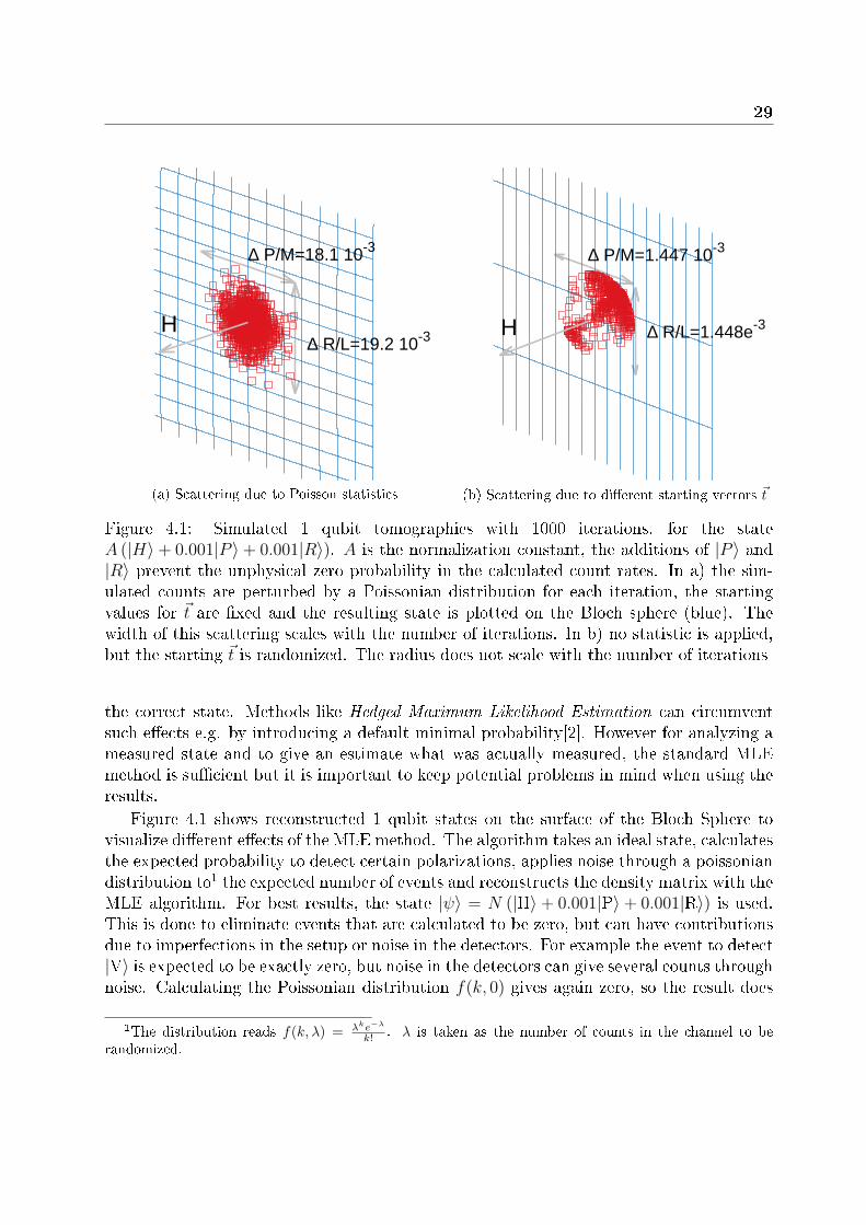
Figure 4.1: Simulated 1 qubit tomographies with 1000 iterations, for the stateA (|H〉+ 0.001|P 〉+ 0.001|R〉). A is the normalization constant, the additions of |P 〉 and|R〉 prevent the unphysical zero probability in the calculated count rates. In a) the sim-ulated counts are perturbed by a Poissonian distribution for each iteration, the startingvalues for ~t are �xed and the resulting state is plotted on the Bloch sphere (blue). Thewidth of this scattering scales with the number of iterations. In b) no statistic is applied,but the starting ~t is randomized. The radius does not scale with the number of iterations

the correct state. Methods like Hedged Maximum Likelihood Estimation can circumventsuch e�ects e.g. by introducing a default minimal probability[2]. However for analyzing ameasured state and to give an estimate what was actually measured, the standard MLEmethod is su�cient but it is important to keep potential problems in mind when using theresults.

Figure 4.1 shows reconstructed 1 qubit states on the surface of the Bloch Sphere tovisualize di�erent e�ects of the MLE method. The algorithm takes an ideal state, calculatesthe expected probability to detect certain polarizations, applies noise through a poissoniandistribution to1 the expected number of events and reconstructs the density matrix with theMLE algorithm. For best results, the state |ψ〉 = N (|H〉+ 0.001|P〉+ 0.001|R〉) is used.This is done to eliminate events that are calculated to be zero, but can have contributionsdue to imperfections in the setup or noise in the detectors. For example the event to detect|V〉 is expected to be exactly zero, but noise in the detectors can give several counts throughnoise. Calculating the Poissonian distribution f(k, 0) gives again zero, so the result does

1The distribution reads f(k, λ) = λke−λ

k! . λ is taken as the number of counts in the channel to berandomized.

30 4. Maximum Likelihood Estimation

not re�ect a real experiment. This is why a state with small admixtures is chosen.The plots show di�erent types of scattering in the reconstructed states. First, there is

scattering that results from the applied statistic, and there is scattering depending on howthe start values of the afore described ~t vector are chosen. Figure 4.1a shows endpointsafter MLE when poissonian noise is added and ~t is kept �x for each run. Compared to thestate vectors that were not optimized through MLE, the overall distance to the ideal statedecreases so the recovered state is on average closer to the original one than the perturbedmeasured. This shows that MLE helps to recover a state that is subject to noise. Figure4.1b shows result where the state was not perturbed by any statistic on the counts butthe starting parameters for the vector ~t are randomized. The overall spread is smaller bya factor 10 compared to the �rst plot so this e�ect will have neglectable impact but itillustrates the dependence of the result on input parameters in the MLE algorithm.

The simulations demonstrate that �tting a state with the above method has e�ectson the recovered state. Despite the previously mentioned problems of the probabilisticinterpretation the routine is able to move all directly (un�tted) state vectors closer to the�real� state, thus creating an improvement over states that are reconstructed without anyoptimization. There are other approaches that try to eliminate the remaining �aws, butso far the relatively simple assumptions and easy formulation make the MLE approach thetool of choice.

5 Experiment

In this part the experimental setup and the underlying processes to create and measurethe 6 qubit symmetric Dicke State are explained.

5.1 Entangled State Production via Spontaneous Para-

metric Down Conversion

The basic process exploited to create entangled photons is Spontaneous Parametric DownConversion (SPDC). Descriptions of this process were �rst published by Madge and Mahr[29] and more elaborate by Byer and Harris [9]. In a nonlinear crystal an incoming photonwith energy ~ω can split in 2 photons with half the energy that have a �xed polariza-tion relation and are therefore entangled. Depending on the crystal type and orientation,di�erent types of polarization and emission directions can be constructed.

Any electromagnetic �eld inside a nonlinear crystal will induce a local polarization ofthe form [43]

P = ε0(χ(1)E + χ(2)E2 + χ(3)E3 + · · ·

)with the permittivity ε0 and χ(n), the nonlinear susceptibility of order n in the medium.Depending on the incident power and the type of material, higher order χ(n) will contribute.If the standard ansatz for an electric �eld E (t) = A cos (ωt) is inserted, the polarizationup to second order in χ becomes

P (t) = ε0χ(1)A cos (ωt) +

1

2ε0χ

(2)A2 [1 + cos (2ωt)]

Considering the �eld in a quantum mode description, the expression shows that a �eld offrequency ω will create another �eld with frequency 2ω. The �rst one (later called pump�eld) will induce local movements of charges which will produce the second �eld, that canbe detected as 2 photons in the distance. The nonlinearity can also be used to generatephotons of de�ned frequencies in up- or down-conversion. Arti�cially imposing 2 �elds, thecreation of photons that have the sum or di�erence in frequency can be stimulated[35].

In this setup light with 390 nm wavelength will be used to create entangled photons of780 nm, so just a single pump �eld is injected in the crystal. In this case, down conversionhappens randomly what gives raise to the �spontaneous� in SPDC. In terms of photons, a

32 5. Experiment

single one of frequency ωp (pump), will decay in 2 photons with frequency ωs (signal) andωi (idler)

1. Energy conservation must hold

ωp = ωs + ωi

as does momentum conservation~kp = ~ks + ~ki (5.1)

The second requirement is also a phase matching condition that needs to be ful�lled tohave output at all[43]. Eventually the centers of 2 creation processes are separated byodd multiples of the wavelength, that would correspond to a phase di�erence of π, sono resulting �eld exits the crystal. Any other phase di�erence than 2π between creationcenters will average out the overall �elds. Thus it is mandatory to have the signal and

idler photons phase matched. Using∣∣∣~k∣∣∣ = ωn

cthe expression

np − ns = (ni − np)ωiωs

(5.2)

can be found. Commonly the refractive index is a function of the frequency ni = n (ωi) andfor the case of normal dispersive media ni ≤ ns ≤ np holds. This shows that (np − ns) ≥ 0and (ni − np) ≤ 0. Therefore there is no general solution to 5.2. There are crystals hathave an increasing refractive index for lower frequencies but due to large energy losses thecommon method is to use birefringent crystals. In the simplest type, the refractive indexdi�ers only for a single propagation direction. This axis is called the optical axis and lightpropagating in this direction experiences the extraordinary refractive index, whereas light inthe perpendicular plane is subject to the ordinary refractive index. There is a discriminationbetween uniaxial positive (ne > no) and uniaxial negative (ne < no) crystals. The pumpphoton must be polarized along the direction with the lowest refractive index. In casesignal and idler photon have the same polarization, the phase matching scheme is calledType I, if they are orthogonal polarized Type II.

Birefringence requires phase matching (eq. 5.1) for all 3 propagation directions sep-

arately. E.g. ωpnp~k = ωini~k + ωsns~k must hold for any ~k ∈{~kp, ~ks, ~ki

}. Calculations

show that the emission of signal and idler photon for Type II phase matching (which isused here) is only full�lled if the emission lies on 2 cones[43](see �gure 5.1). Aperture andcenter can be in�uenced by the angle of the crystal relative to the pump beam. Tilting,also called angle tuning, allows �ne adjustment of the matching condition. If the onlyintersection is a single line, the setup is called collinear, con�gurations with 2 intersectionsare called non-collinear. Because the signal photon is emitted on the surface of one cone,the idler on the other, collecting the light that the intersection of both will result in anentangled state of the type

1√2

(|HV〉+ eiφ|VH〉

)1The nomenclature has historical reasons

5.2 The Symmetric Dicke State 33

ω1= 2ω

2

ω2

ω2

Type II BBO

H

V

entangledphotons

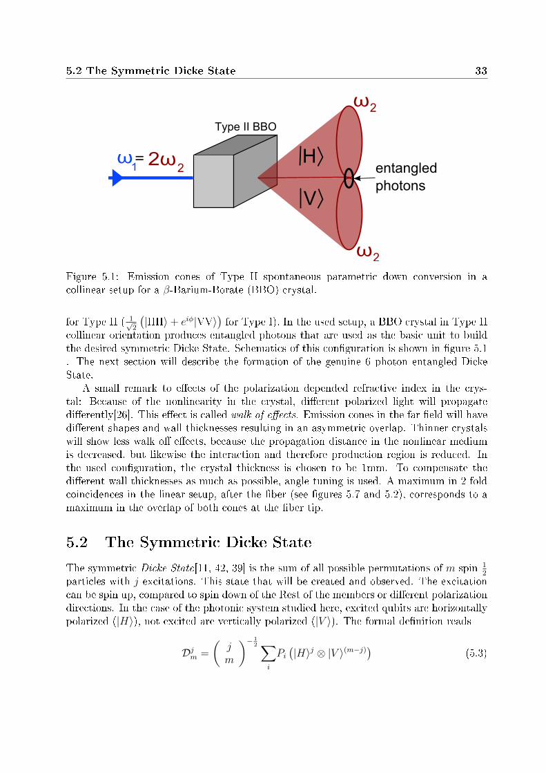
Figure 5.1: Emission cones of Type II spontaneous parametric down conversion in acollinear setup for a β-Barium-Borate (BBO) crystal.

for Type II ( 1√2

(|HH〉+ eiφ|VV〉

)for Type I). In the used setup, a BBO crystal in Type II

collinear orientation produces entangled photons that are used as the basic unit to buildthe desired symmetric Dicke State. Schematics of this con�guration is shown in �gure 5.1. The next section will describe the formation of the genuine 6 photon entangled DickeState.

A small remark to e�ects of the polarization depended refractive index in the crys-tal: Because of the nonlinearity in the crystal, di�erent polarized light will propagatedi�erently[26]. This e�ect is called walk of e�ects. Emission cones in the far �eld will havedi�erent shapes and wall thicknesses resulting in an asymmetric overlap. Thinner crystalswill show less walk o� e�ects, because the propagation distance in the nonlinear mediumis decreased, but likewise the interaction and therefore production region is reduced. Inthe used con�guration, the crystal thickness is chosen to be 1mm. To compensate thedi�erent wall thicknesses as much as possible, angle tuning is used. A maximum in 2 foldcoincidences in the linear setup, after the �ber (see �gures 5.7 and 5.2), corresponds to amaximum in the overlap of both cones at the �ber tip.

5.2 The Symmetric Dicke State

The symmetric Dicke State[11, 42, 39] is the sum of all possible permutations of m spin 12

particles with j excitations. This state that will be created and observed. The excitationcan be spin up, compared to spin down of the Rest of the members or di�erent polarizationdirections. In the case of the photonic system studied here, excited qubits are horizontallypolarized (|H〉), not excited are vertically polarized (|V 〉). The formal de�nition reads

Djm =

(jm

)− 12 ∑

i

Pi(|H〉j ⊗ |V 〉(m−j)

)(5.3)

34 5. Experiment

where {Pi} are all permutations of the expression in the brackets and |H〉n = |H〉⊗n =⊗n|H〉. In this experiment, the state D3

6 will be crate and observed. Its terms have he

polarization con�gurations

HHHVVV HHVHVV HHVVHV HHVVVH

HVHHVV HVHVHV HVHVVH HVVHHV

HVVHVH HVVVHH VHHHVV VHHHVV

VHHVHV VHHVVH VHVHVH VHVVHH

VVHHHV VVHHVH VVHVHH VVVHHH

It is chosen, because a loss of photons is not equivalent with the loss of entangle-ment, and common other states, like the W-state or GHZ state can be created by localprojections[13]. This allows a general experiment that can easily been expanded to otherstates.

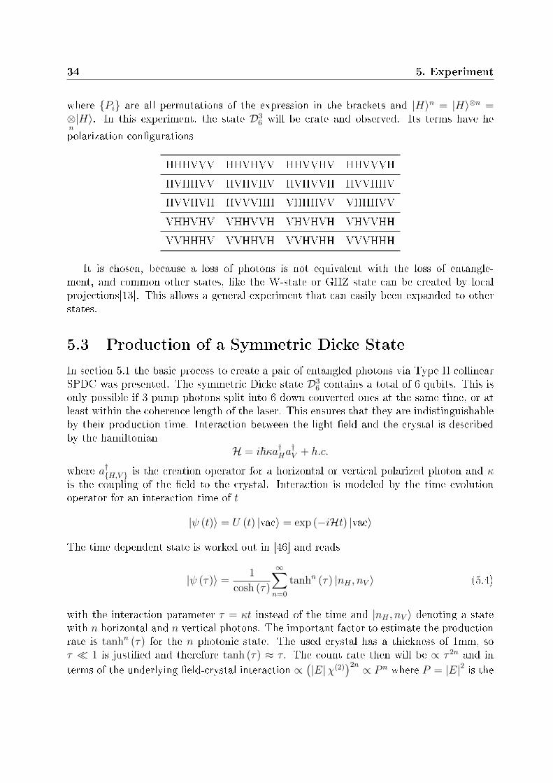
5.3 Production of a Symmetric Dicke State

In section 5.1 the basic process to create a pair of entangled photons via Type II collinearSPDC was presented. The symmetric Dicke state D3

6 contains a total of 6 qubits. This isonly possible if 3 pump photons split into 6 down converted ones at the same time, or atleast within the coherence length of the laser. This ensures that they are indistinguishableby their production time. Interaction between the light �eld and the crystal is describedby the hamiltonian

H = i~κa†Ha†V + h.c.

where a†{H,V } is the creation operator for a horizontal or vertical polarized photon and κis the coupling of the �eld to the crystal. Interaction is modeled by the time evolutionoperator for an interaction time of t

|ψ (t)〉 = U (t) |vac〉 = exp (−iHt) |vac〉

The time dependent state is worked out in [46] and reads

|ψ (τ)〉 =1

cosh (τ)

∞∑n=0

tanhn (τ) |nH , nV 〉 (5.4)

with the interaction parameter τ = κt instead of the time and |nH , nV 〉 denoting a statewith n horizontal and n vertical photons. The important factor to estimate the productionrate is tanhn (τ) for the n photonic state. The used crystal has a thickness of 1mm, soτ � 1 is justi�ed and therefore tanh (τ) ≈ τ . The count rate then will be ∝ τ 2n and in

terms of the underlying �eld-crystal interaction ∝(|E|χ(2)

)2n ∝ P n where P = |E|2 is the

5.3 Production of a Symmetric Dicke State 35

interferencefilter

50:50

66:33

66:33

50:50

50:50

from source

16.6%

16.6%

16.6%

16.6%

16.6%16.6%

(a) Ideal splitting ratio

interferencefilter

1.08

0.49

0.51

0.95

0.90

from source

17%

15.8%

17.5%

15.8%

15%

15%

(b) Measured splitting ratio in the experiment.

Figure 5.2: Linear setup to prepare the Symmetric Dicke State in its ideal and real form.From the source a bunch of 6 entangled photons is fed into the setup. The (ideal) polar-ization independent beam splitters distribute equal beam intensity into each arm. For thecase that each photon splits into a di�erent arm, the state can be observed. The triggeris a simultaneous photon event in each of the blue analysis blocks. a) shows the idealsplitting ratio with an expected intensity of 16.6% of the original in each arm. b) showsthe measured splitting ratios and intensity distributions. 33 : 66 = 0.5 and 50 : 50 = 1would be expected; overall 3.73% are lost.

power of the �eld inside the crystal. More power will help dramatically. For example anincrease of the power by 1% will result in 6% higher production rates, 2% in 12% moreand so on; the high exponent has a big impact here.

To observe the Symmetric Dicke State, the 6 photons that form the state have tobe separated spatially, otherwise the above described tomographic scheme would not beapplicable, as local measurements are not possible. In addition the coherence length mustbe longer than the depth of the crystal, that the place of production cannot be resolved[24].This is achieved by a narrow bandgab �lter that reduces the uncertainty of the wavelengthand increases the coherence length.

Spatial separation is realized through probabilistic splitting of light from the source inseparated arms. Such a setup is called a linear optical setup. In the case of 6 qubits, 6arms are needed as illustrated in �gure 5.2a . Ideally, the beam splitters are polarizationmaintaining and distribute equal intensity (16.6̄%) into all arms. This is achieved with 350:50, and 2 33:66 splitters. A Field Programmable Gate Array (FGPA) counts concurrentevents in the arms. If 6 photons were detected simultaneously in all arms, the eventcan be counted to be a 6 photon event. This method is called post selection, becausemore data are recorded than used. For example all 4 fold events are stored as well butdiscarded in the evaluation. Also, all arms must have the same length, because otherwise

36 5. Experiment

HWP QWP

Source

50:50 PBS

CoincidenceLogic

H

H

V

V

2

1

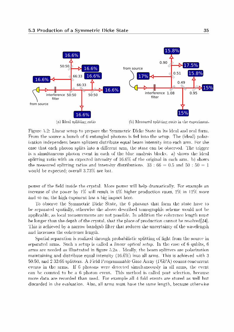
Figure 5.3: Analysis of a 2 qubit state. If a photon is detected in arm 1 and 2 simultane-ously, a 2 photon state has been detected.

photons entering the setup concurrently, will be detected at di�erent times, destroying the6 fold event pattern. To extract probabilities of the type P|XY ZXY Z〉, the counts from theFPGA are used. An example wiring for 2 qubits is shown in �gure 5.3. The part that ishighlighted by blue surroundings is an analysis block like in 5.3. In the example, possiblecounts originate from HH, HV, VH and VV events for which P|HH〉, P|HV 〉, P|V H〉 and P|V V 〉can be calculated. For an arbitrary state of N qubits, 2N coincidence combinations arepossible.

A downside of the linear setup is its e�ciency in distributing the photons �correctly�.From the produced packs of 6 photons, only 6!

66≈ 1.54% can be detected via coincidences

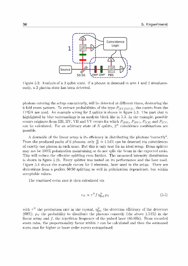
of exactly one photon in each arms. But this is only true for an ideal setup. Beam splittermay not be 100% polarization maintaining or do not split the beam in the expected ratio.This will reduce the e�ective splitting even further. The measured intensity distributionis shown in �gure 5.2b. Every splitter was tested on its performance and the best used.Figure 5.4 shows the example curves for 2 elements, later used in the setup. There arederivations from a perfect 50:50 splitting as well in polarization dependence, but withinacceptable values.

The combined event rate is then calculated via

eN ∝ τNf ηNDet

pN (5.5)

with τN the production rate in the crystal, ηNDet

the detection e�ciency of the detectors(60%), pN the probability to distribute the photons correctly (the above 1.54%) in thelinear setup and f , the repetition frequency of the pulsed laser (80.8Hz). From recordedevent rates, the proportionality factor within τ can be calculated and then the estimatedevent rate for higher or lower order events extrapolated.

5.4 Higher order noise of D36 37

0.44

0.46

0.48

0.5

0.52

0.54

0.56

0.58

H 20 40 60 80 V 100 120 140 160 H 0.44

0.46

0.48

0.5

0.52

0.54

0.56

0.58

Tra

nsm

issi

on [

% o

f bea

m]

Ref

lexi

on [%

of ]

Incomming polarization [degrees]

Splitting dependence on the incident polarization

Transmission BS 1Reflexion BS 1

Transmission BS 2Reflexion BS 2

Figure 5.4: Transmission and Re�exion of the �rst beam splitter in 5.2 and another samplefrom the same batch for di�erent incident polarizations. Although the splitting is not ideal50 : 50, the polarization is preserved. The di�erences between the 2 samples are small butthe ones used in the setup are chosen to be the best in terms of polarization stability andsplitting ratio.

5.4 Higher order noise of D36

Noise can be produced by imperfections in the detectors that lead to counts when no photonwas present or a photon was present but no event was triggered. In case of symmetric states,a special type is produced through loss of photons. Formula 5.4 shows that the number ofphotons in a produced state depends on the laser power inside the crystal. Besides 2 foldstates, also 4,6,8 etc. ones are created, although with much lower probability.

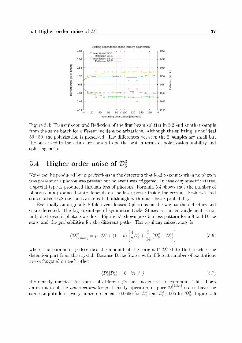
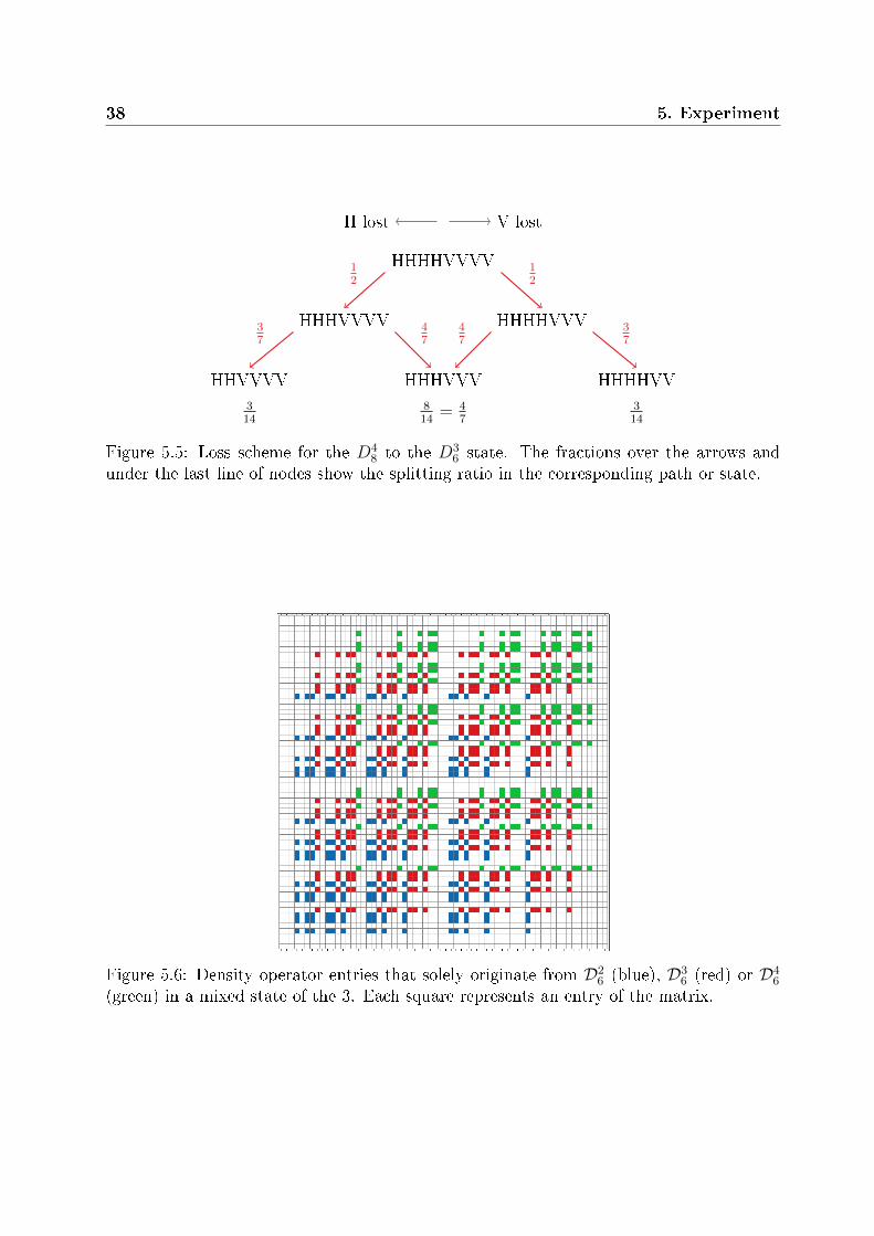
Eventually an originally 8 fold event looses 2 photons on the way to the detectors and6 are detected. The big advantage of symmetric Dicke States is that entanglement is notfully destroyed if photons are lost. Figure 5.5 shows possible loss pattern for a 8 fold Dickestate and the probabilities for the di�erent paths. The resulting mixed state is

(D3

6

)noisy

= p · D36 + (1− p)

[4

7D3

6 +3

14

(D2

6 +D46

)](5.6)

where the parameter p describes the amount of the �original� D36 state that reaches the

detection part from the crystal. Because Dicke States with di�erent number of excitationsare orthogonal on each other

〈Di6|Dj6〉 = 0 ∀i 6= j (5.7)

the density matrices for states of di�erent j's have no entries in common. This allowsan estimate of the noise parameter p. Density operators of pure D{2,3,4}6 states have thesame amplitude in every nonzero element; 0.0666̄ for D2

6 and D46, 0.05 for D3

6. Figure 5.6

38 5. Experiment

HHHHVVVV

HHHVVVV HHHHVVV

HHHVVVHHVVVV HHHHVV

H lost V lost

12

12

37

47

47

37

314

814

= 47

314

Figure 5.5: Loss scheme for the D48 to the D3

6 state. The fractions over the arrows andunder the last line of nodes show the splitting ratio in the corresponding path or state.

Figure 5.6: Density operator entries that solely originate from D26 (blue), D3

6 (red) or D46

(green) in a mixed state of the 3. Each square represents an entry of the matrix.

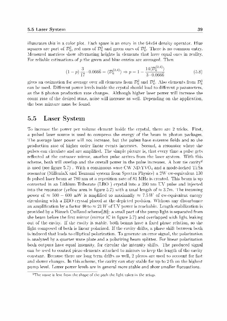
5.5 Laser System 39

illustrates this in a color plot. Each spare is an entry in the 64x64 density operator. Bluesquares are part of D2

6, red ones of D36 and green ones of D4

6. There is no common entry.Measured matrices show alternating heights in elements that have equal ones in reality.For reliable estimations of p the green and blue entries are averaged. Then

(1− p) 3

17· 0.0666̄ = 〈D{2,4}6 〉 ⇒ p = 1− 14〈D{2,4}6 〉

3 · 0.0666̄(5.8)

gives an estimation for average over all elements from D26 and D4

6. Also elements from D36

can be used. Di�erent power levels inside the crystal should lead to di�erent p parameters,as the 8 photon production rate changes. Although higher laser power will increase thecount rate of the desired state, noise will increase as well. Depending on the application,the best mixture must be found.

5.5 Laser System

To increase the power per volume element inside the crystal, there are 2 tricks. First,a pulsed laser source is used to compress the energy of the beam in photon packages.The average laser power will not increase, but the pulses have extreme �elds and so theproduction rate of higher order linear events increases. Second, a resonator where thepulses can circulate and are ampli�ed. The simple picture is, that every time a pulse getsre�ected at the entrance mirror, another pulse arrives from the laser system. With thisscheme, both will overlap and the overall power in the pulse increases. A bow tie cavity2

is used (see �gure 5.7) . With a continuous wave CW ND:YVO4 and a mode-locked Ti:Saresonator (MilleniaX and Tsunami system from Spectra Physics) a 2W cw-equivalent 130fs pulsed laser beam at 780 nm at a repetition rate of 81 MHz is created. This beam is upconverted in an Lithium Triborate (LBO ) crystal into a 390 nm UV pulse and injectedinto the resonator (yellow area in �gure 5.7) with a total length of ≈ 3.7m. The incomingpower of ≈ 500 − 600 mW is ampli�ed to maximally ≈ 7.5W of cw-equivalent energycirculating with a BBO crystal placed at the depicted position. Without any disturbancean ampli�cation by a factor 40 to ≈ 21W of UV power is reachable. Length stabilization isprovided by a Hänsch Cuillaud scheme[20]: a small part of the pump light is separated fromthe beam before the �rst mirror (mirror IC in �gure 5.7) and overlapped with light leakingout of the cavity. If the cavity is stable, both beams have a �xed phase relation, so thelight composed of both is linear polarized. If the cavity drifts, a phase shift between bothis induced that leads to elliptical polarization. To generate an error signal, the polarizationis analyzed by a quarter wave plate and a polarizing beam splitter. For linear polarizationboth outputs have equal intensity, for circular the intensity shifts. The produced signalcan be used to control piezo elements attached to mirrors to keep the length of the cavityconstant. Because there are long term drifts as well, 2 piezos are used to account for fastand slower changes. In this scheme, the cavity can stay stable for up to 24h on the highestpump level. Lower power levels are in general more stable and show smaller �uctuations.

2The name is lent from the shape of the path the light takes in the setup.

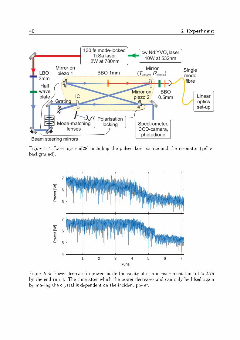
40 5. Experiment

130 fs mode-lockedTi:Sa laser

2W at 780nm

LBO3mm

Beam steering mirrors

BBO 1mmSinglemodefibre

Grating

Mirror onpiezo 1

Mirror onpiezo 2

Polarisationlocking

Halfwaveplate

( , )T R780nm 390nm

BBO0.5mm

Mode-matchinglenses

IC

Spectrometer,CCD-camera,

photodiode

cw Nd:YVO laser

10W at 532nm4

Mirror

Linearopticsset-up

Figure 5.7: Laser system[28] including the pulsed laser source and the resonator (yellowbackground).

5

6

7

Pow

er [W

]

4

5

6

7

1 2 3 4 5 6 7

Pow

er [W

]

Runs

Figure 5.8: Power decrease in power inside the cavity after a measurement time of ≈ 2.7hby the end run 4. The time after which the power decreases and can only be lifted againby moving the crystal is dependent on the incident power.

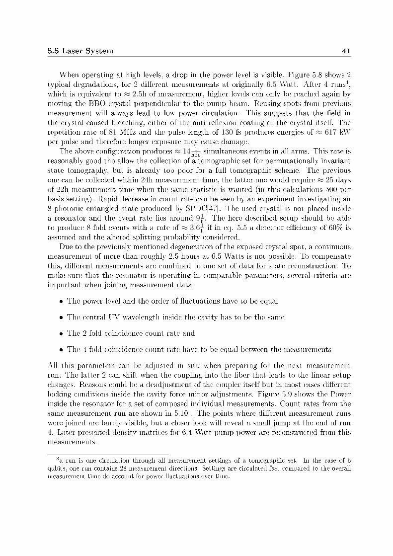
5.5 Laser System 41

When operating at high levels, a drop in the power level is visible. Figure 5.8 shows 2typical degradations, for 2 di�erent measurements at originally 6.5 Watt. After 4 runs3,which is equivalent to ≈ 2.5h of measurement, higher levels can only be reached again bymoving the BBO crystal perpendicular to the pump beam. Reusing spots from previousmeasurement will always lead to low power circulation. This suggests that the �eld inthe crystal caused bleaching, either of the anti re�exion coating or the crystal itself. Therepetition rate of 81 MHz and the pulse length of 130 fs produces energies of ≈ 617 kWper pulse and therefore longer exposure may cause damage.

The above con�guration produces ≈ 14 1min

simultaneous events in all arms. This rate isreasonably good tho allow the collection of a tomographic set for permutationally invariantstate tomography, but is already too poor for a full tomographic scheme. The previousone can be collected within 24h measurement time, the latter one would require ≈ 25 daysof 22h measurement time when the same statistic is wanted (in this calculations 500 perbasis setting). Rapid decrease in count rate can be seen by an experiment investigating an8 photonic entangled state produced by SPDC[47]. The used crystal is not placed insidea resonator and the event rate lies around 9 1

h. The here described setup should be able

to produce 8 fold events with a rate of ≈ 3.6 1hif in eq. 5.5 a detector e�ciency of 60% is

assumed and the altered splitting probability considered.Due to the previously mentioned degeneration of the exposed crystal spot, a continuous

measurement of more than roughly 2.5 hours at 6.5 Watts is not possible. To compensatethis, di�erent measurements are combined to one set of data for state reconstruction. Tomake sure that the resonator is operating in comparable parameters, several criteria areimportant when joining measurement data:

� The power level and the order of �uctuations have to be equal

� The central UV wavelength inside the cavity has to be the same

� The 2 fold coincidence count rate and

� The 4 fold coincidence count rate have to be equal between the measurements

All this parameters can be adjusted in situ when preparing for the next measurementrun. The latter 2 can shift when the coupling into the �ber that leads to the linear setupchanges. Reasons could be a deadjustment of the coupler itself but in most cases di�erentlocking conditions inside the cavity force minor adjustments. Figure 5.9 shows the Powerinside the resonator for a set of composed individual measurements. Count rates from thesame measurement run are shown in 5.10 . The points where di�erent measurement runswere joined are barely visible, but a closer look will reveal a small jump at the end of run4. Later presented density matrices for 6.4 Watt pump power are reconstructed from thismeasurements.

3a run is one circulation through all measurement settings of a tomographic set. In the case of 6qubits, one run contains 28 measurement directions. Settings are circulated fast compared to the overallmeasurement time do account for power �uctuations over time.

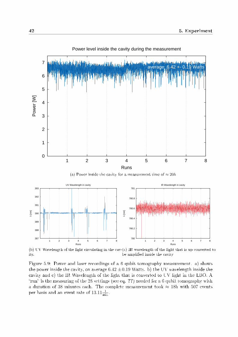
42 5. Experiment

0

1

2

3

4

5

6

7

1 2 3 4 5 6 7 8

Pow

er [W

]

Runs

Power level inside the cavity during the measurement

average: 6.42 +- 0.19 Watts

(a) Power inside the cavity for a measurement time of ≈ 20h

387

388

389

390

391

392

393

1 2 3 4 5 6 7 8

λ [n

m]

Runs

UV Wavelength in cavity

(b) UV Wavelength of the light circulating in the cav-ity.

780

780.2

780.4

780.6

780.8

781

1 2 3 4 5 6 7 8

λ [n

m]

Runs

IR Wavelength in cavity

(c) IR wavelength of the light that is up converted tobe ampli�ed inside the cavity

Figure 5.9: Power and laser recordings of a 6 qubit tomography measurement. a) showsthe power inside the cavity, on average 6.42 ±0.19 Watts. b) the UV wavelength inside thecavity and c) the IR Wavelength of the light that is converted to UV light in the LBO. A�run� is the measuring of the 28 settings (see eq. ??) needed for a 6 qubit tomography witha duration of 38 minutes each. The complete measurement took ≈ 18h with 507 eventsper basis and an event rate of 13.11 1

min.

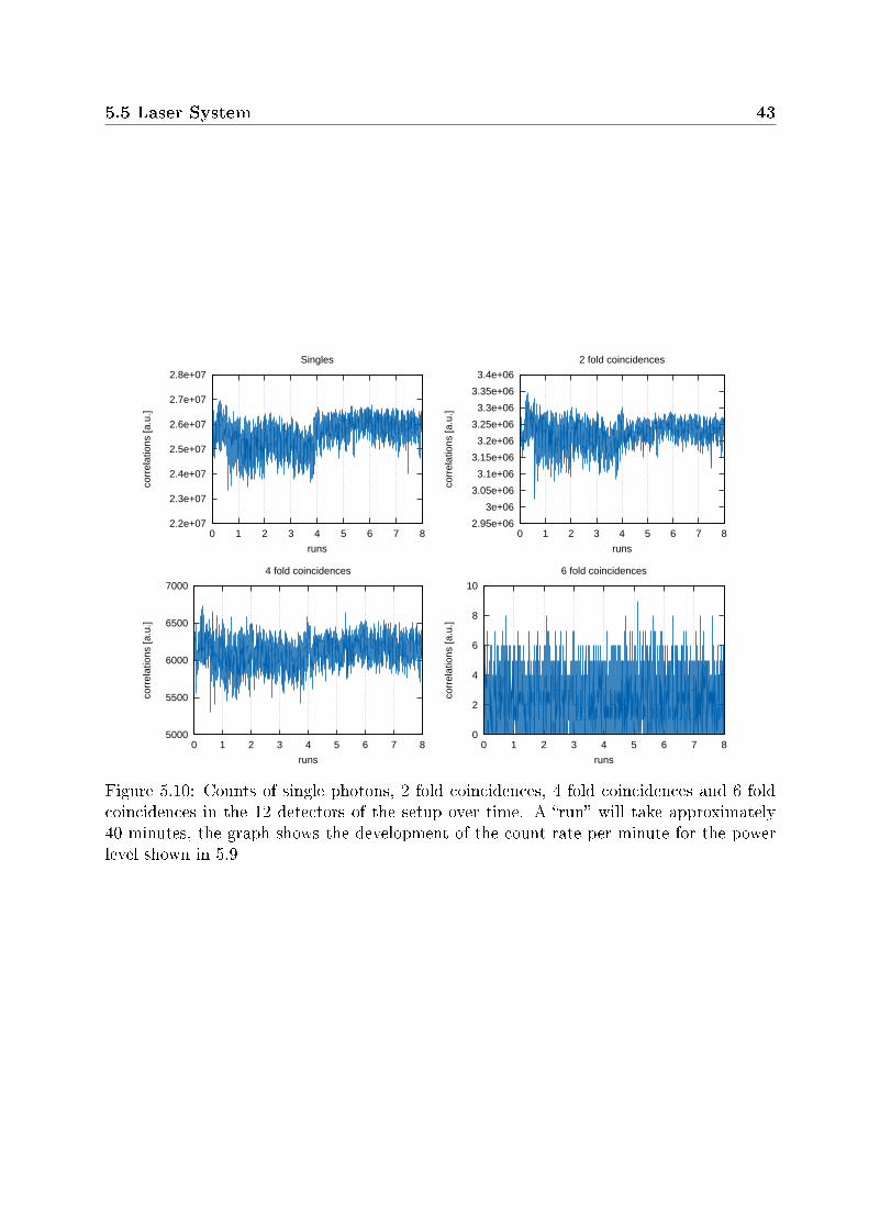
5.5 Laser System 43

2.2e+07

2.3e+07

2.4e+07

2.5e+07

2.6e+07

2.7e+07

2.8e+07

0 1 2 3 4 5 6 7 8

corr

elat

ions

[a.u

.]

runs

Singles

2.95e+06

3e+06

3.05e+06

3.1e+06

3.15e+06

3.2e+06

3.25e+06

3.3e+06

3.35e+06

3.4e+06

0 1 2 3 4 5 6 7 8

corr

elat

ions

[a.u

.]

runs

2 fold coincidences

5000

5500

6000

6500

7000

0 1 2 3 4 5 6 7 8

corr

elat

ions

[a.u

.]

runs

4 fold coincidences

0

2

4

6

8

10

0 1 2 3 4 5 6 7 8

corr

elat

ions

[a.u

.]

runs

6 fold coincidences

Figure 5.10: Counts of single photons, 2 fold coincidences, 4 fold coincidences and 6 foldcoincidences in the 12 detectors of the setup over time. A �run� will take approximately40 minutes, the graph shows the development of the count rate per minute for the powerlevel shown in 5.9

44 5. Experiment

6 State Tomography of the 6 qubit

symmetric Dicke State

This section discusses the results investigating the symmetric Dicke State produced bythe described laser system and linear setup. The above explained methods are used toextract the density matrix from measured counts and to compare the observed state to anexpected, ideal Dicke State.

6.1 Symmetric Overlap

For PI tomography, a set of 28 measurement directions (see eq. 3.8 and �gure 3.2) needs tobe measured. To make an estimate on the overlap with the (PI) symmetric subspace of thestate, directions X⊗6, Y ⊗6 and Z⊗6 are included to make use of eq. 22. In the following, 2measurements, one at 6.4 the other at 3.7 Watt laser power, are discussed. Their overlapwith the symmetric subspace is calculated to be

overlap

P = 3.7 Watt 0.9162

P = 6.4 Watt 0.8868

It is important to note that eq. 3.9 is designed to give 1 for D36 and behave like a distance

measure for other states. To be precise, not a general overlap with the (PI) symmetricsubspace is calculated, but the overlap with the symmetric subspace of D3

6. In chapter 5.4noise that is created from higher order events in the crystal is analyzed. This e�ects willlead to a mixed Dicke State, which has contributions from D2

6 and D46. Using eq. 3.9 on

these states gives 0.75 each and therefore the estimate for the complete state will decrease.Anticipating results for the amount of noise from chapter 6.4, values of 0.916 for 3.7 Wattand 0.925 for 6.4 Watt are expected. This is in good agreement with the measured one.Because D2

6 and D46 are PI symmetric, the 28 basis scheme can be used.

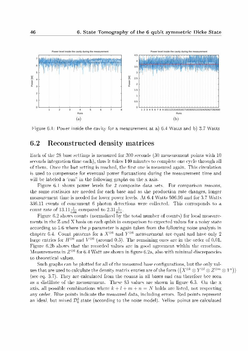
46 6. State Tomography of the 6 qubit symmetric Dicke State

0

1

2

3

4

5

6

7

1 2 3 4 5 6 7 8

Pow

er [W

]

Runs

Power level inside the cavity during the measurement

average: 6.42 +- 0.19 Watts

(a)

0

0.5

1

1.5

2

2.5

3

3.5

4

4.5

1 2 3 4 5 6 7 8 9 101112131415161718192021222324252627282930

Pow

er [W

]

Runs

Power level inside the cavity during the measurement

average: 3.73 +- 0.2 Watts

(b)

Figure 6.1: Power inside the cavity for a measurement at a) 6.4 Watts and b) 3.7 Watts

6.2 Reconstructed density matrices

Each of the 28 base settings is measured for 300 seconds (30 measurement points with 10seconds integration time each), thus it takes 140 minutes to complete one cycle through allof them. Once the last setting is reached, the �rst one is measured again. This circulationis used to compensate for eventual power �uctuations during the measurement time andwill be labeled a �run� in the following graphs on the x axis.

Figure 6.1 shows power levels for 2 composite data sets. For comparison reasons,the same statistics are needed for each base and as the production rate changes, longermeasurement time is needed for lower power levels. At 6.4 Watts 506.96 and for 3.7 Watts336.11 events of concurrent 6 photon detections were collected. This corresponds to acount rate of 13.11 1

mincompared to 2.31 1

min.

Figure 6.2 shows counts (normalized by the total number of counts) for local measure-ments in the Z and X basis on each qubit in comparison to expected values for a noisy stateaccording to 5.6 where the p parameter is again taken from the following noise analysis inchapter 6.4. Count patterns for a X⊗6 and Y ⊗6 measurement are equal and have only 2large entries for H⊗6 and V ⊗6 (around 0.3). The remaining ones are in the order of 0.01.Figure 6.2b shows that the recorded values are in good agreement within the errorbars.Measurements in Z⊗6 for 6.4 Watt are shown in �gure 6.2a, also with minimal discrepanciesto theoretical values.

Such graphs can be plotted for all of the measured base con�gurations, but the only val-ues that are used to calculate the density matrix entries are of the form 〈

(X⊗k ⊗ Y ⊗l ⊗ Z⊗m ⊗ 1

n)〉

(see eq. 3.7). They are calculated from the counts in all bases and can therefore bee seenas a distillate of the measurement. These 83 values are shown in �gure 6.3. On the xaxis, all possible combinations where k + l + m + n = N holds are listed, not respectingany order. Blue points indicate the measured data, including errors. Red points representan ideal, but mixed D3

6 state (according to the noise model). Yellow points are calculated

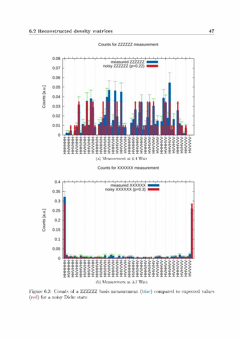
6.2 Reconstructed density matrices 47

0

0.01

0.02

0.03

0.04

0.05

0.06

0.07

0.08H

HH

HH

HH

VH

HH

HH

HV

HH

HH

VV

HH

HH

HH

VH

HH

VH

VH

HH

HV

VH

HH

VV

VH

HH

HH

HV

HH

VH

HV

HH

HV

HV

HH

VV

HV

HH

HH

VV

HH

VH

VV

HH

HV

VV

HH

VV

VV

HH

HH

HH

VH

VH

HH

VH

HV

HH

VH

VV

HH

VH

HH

VH

VH

VH

VH

VH

HV

VH

VH

VV

VH

VH

HH

HV

VH

VH

HV

VH

HV

HV

VH

VV

HV

VH

HH

VV

VH

VH

VV

VH

HV

VV

VH

VV

VV

V

Cou

nts

[a.u

.]Counts for ZZZZZZ measurement

measured ZZZZZZnoisy ZZZZZZ (p=0.22)

(a) Measurement at 6.4 Watt

0

0.05

0.1

0.15

0.2

0.25

0.3

0.35

0.4

HH

HH

HH

HV

HH

HH

HH

VH

HH

HV

VH

HH

HH

HV

HH

HV

HV

HH

HH

VV

HH

HV

VV

HH

HH

HH

VH

HV

HH

VH

HH

VH

VH

HV

VH

VH

HH

HV

VH

HV

HV

VH

HH

VV

VH

HV

VV

VH

HH

HH

HV

HV

HH

HV

HH

VH

HV

HV

VH

HV

HH

HV

HV

HV

HV

HV

HH

VV

HV

HV

VV

HV

HH

HH

VV

HV

HH

VV

HH

VH

VV

HV

VH

VV

HH

HV

VV

HV

HV

VV

HH

VV

VV

HV

VV

VV

Cou

nts

[a.u

.]

Counts for XXXXXX measurement

measured XXXXXXnoisy XXXXXX (p=0.3)

(b) Measurement at 3.7 Watt

Figure 6.2: Counts of a ZZZZZZ basis measurement (blue) compared to expected values(red) for a noisy Dicke state

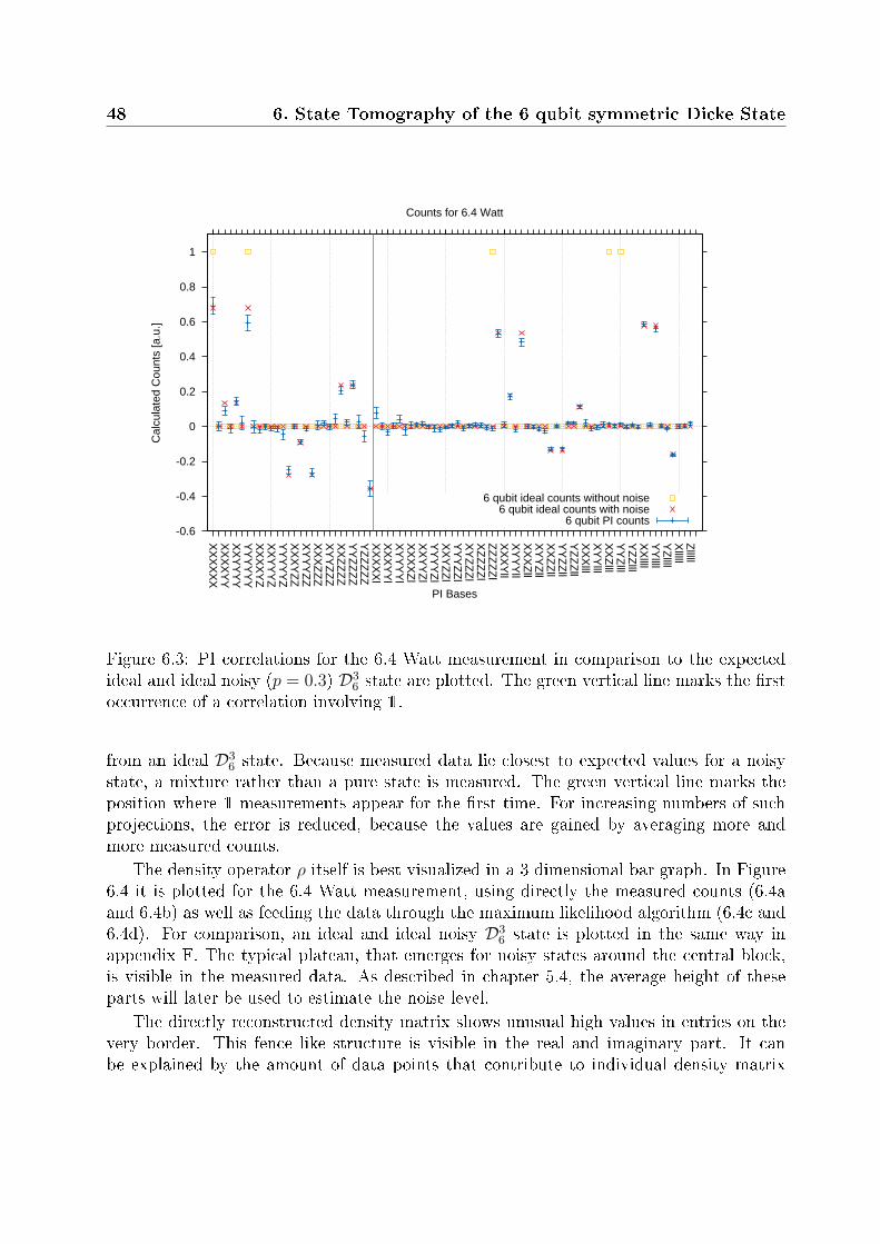
48 6. State Tomography of the 6 qubit symmetric Dicke State

-0.6

-0.4

-0.2

0

0.2

0.4

0.6

0.8

1

XX

XX

XX

XX

XX

YY

XX

YY

YY

YY

YY

YY

XX

XX

YZ

XX

YY

YZ

YY

YY

YZ

XX

XY

ZZ

XY

YY

ZZ

XX

XZ

ZZ

XY

YZ

ZZ

XX

ZZ

ZZ

YY

ZZ

ZZ

YZ

ZZ

ZZ

XX

XX

Xl

XX

XY

Yl

XY

YY

Yl

XX

XX

Zl

XX

YY

Zl

YY

YY

Zl

XX

YZ

Zl

YY

YZ

Zl

XY

ZZ

Zl

XZ

ZZ

Zl

ZZ

ZZ

Zl

XX

XY

llX

YY

Yll

XX

XZ

llX

YY

Zll

XX

ZZ

llY

YZ

Zll

YZ

ZZ

llX

XX

lllX

YY

lllX

XZ

lllY

YZ

lllY

ZZ

lllX

Xllll

YY

llllY

Zllll

Xlllll

Zlllll

Cal

cula

ted

Cou

nts

[a.u

.]

PI Bases

Counts for 6.4 Watt

6 qubit ideal counts without noise6 qubit ideal counts with noise

6 qubit PI counts

Figure 6.3: PI correlations for the 6.4 Watt measurement in comparison to the expectedideal and ideal noisy (p = 0.3) D3

6 state are plotted. The green vertical line marks the �rstoccurrence of a correlation involving 1.

from an ideal D36 state. Because measured data lie closest to expected values for a noisy

state, a mixture rather than a pure state is measured. The green vertical line marks theposition where 1 measurements appear for the �rst time. For increasing numbers of suchprojections, the error is reduced, because the values are gained by averaging more andmore measured counts.

The density operator ρ itself is best visualized in a 3 dimensional bar graph. In Figure6.4 it is plotted for the 6.4 Watt measurement, using directly the measured counts (6.4aand 6.4b) as well as feeding the data through the maximum likelihood algorithm (6.4c and6.4d). For comparison, an ideal and ideal noisy D3

6 state is plotted in the same way inappendix F. The typical plateau, that emerges for noisy states around the central block,is visible in the measured data. As described in chapter 5.4, the average height of theseparts will later be used to estimate the noise level.

The directly reconstructed density matrix shows unusual high values in entries on thevery border. This fence like structure is visible in the real and imaginary part. It canbe explained by the amount of data points that contribute to individual density matrix

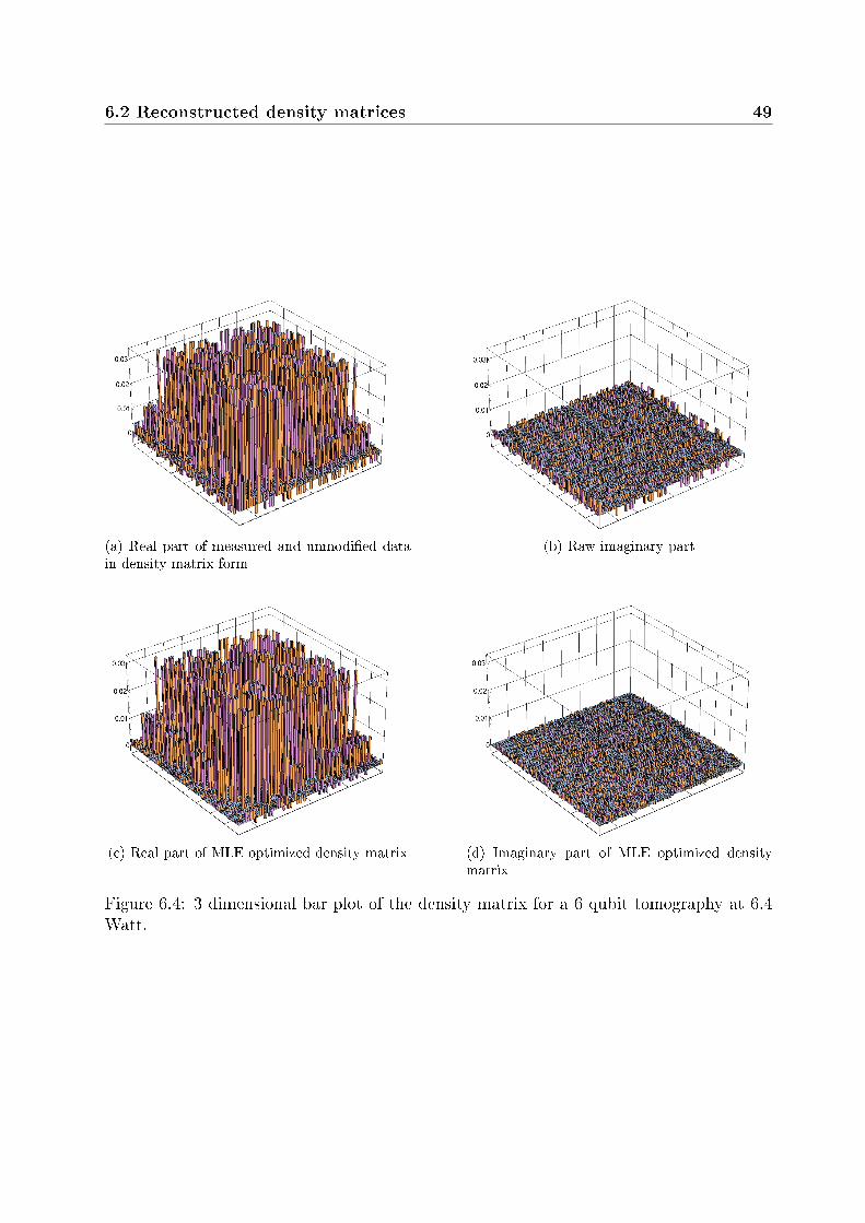
6.2 Reconstructed density matrices 49

(a) Real part of measured and unmodi�ed datain density matrix form

(b) Raw imaginary part

(c) Real part of MLE optimized density matrix (d) Imaginary part of MLE optimized densitymatrix

Figure 6.4: 3 dimensional bar plot of the density matrix for a 6 qubit tomography at 6.4Watt.

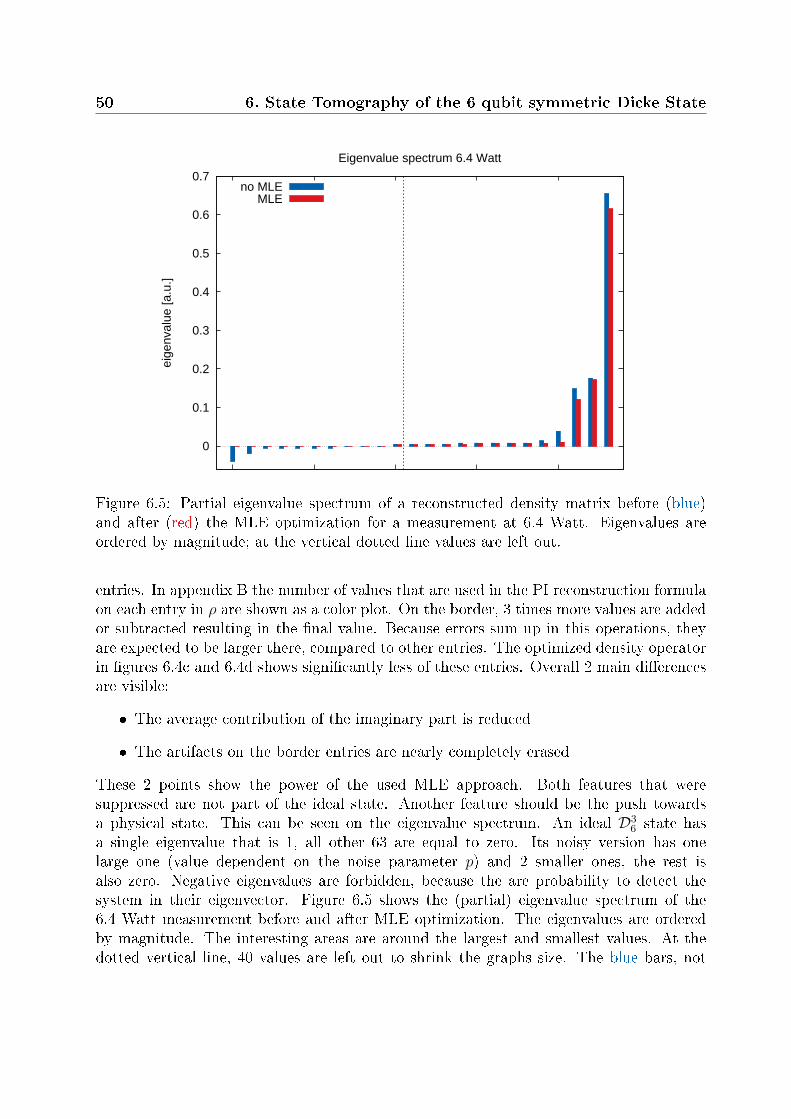
50 6. State Tomography of the 6 qubit symmetric Dicke State

0

0.1

0.2

0.3

0.4

0.5

0.6

0.7ei

genv

alue

[a.u

.]Eigenvalue spectrum 6.4 Watt

no MLEMLE

Figure 6.5: Partial eigenvalue spectrum of a reconstructed density matrix before (blue)and after (red) the MLE optimization for a measurement at 6.4 Watt. Eigenvalues areordered by magnitude; at the vertical dotted line values are left out.

entries. In appendix B the number of values that are used in the PI reconstruction formulaon each entry in ρ are shown as a color plot. On the border, 3 times more values are addedor subtracted resulting in the �nal value. Because errors sum up in this operations, theyare expected to be larger there, compared to other entries. The optimized density operatorin �gures 6.4c and 6.4d shows signi�cantly less of these entries. Overall 2 main di�erencesare visible:

� The average contribution of the imaginary part is reduced

� The artifacts on the border entries are nearly completely erased

These 2 points show the power of the used MLE approach. Both features that weresuppressed are not part of the ideal state. Another feature should be the push towardsa physical state. This can be seen on the eigenvalue spectrum. An ideal D3

6 state hasa single eigenvalue that is 1, all other 63 are equal to zero. Its noisy version has onelarge one (value dependent on the noise parameter p) and 2 smaller ones, the rest isalso zero. Negative eigenvalues are forbidden, because the are probability to detect thesystem in their eigenvector. Figure 6.5 shows the (partial) eigenvalue spectrum of the6.4 Watt measurement before and after MLE optimization. The eigenvalues are orderedby magnitude. The interesting areas are around the largest and smallest values. At thedotted vertical line, 40 values are left out to shrink the graphs size. The blue bars, not

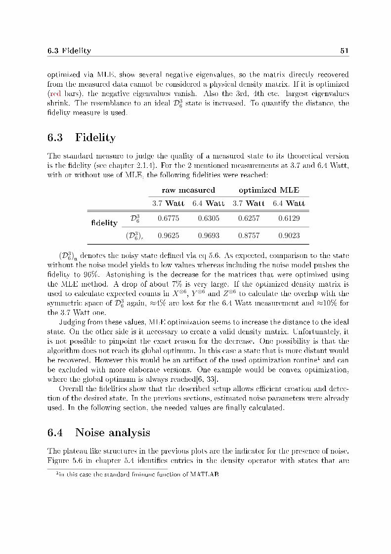
6.3 Fidelity 51

optimized via MLE, show several negative eigenvalues, so the matrix directly recoveredfrom the measured data cannot be considered a physical density matrix. If it is optimized(red bars), the negative eigenvalues vanish. Also the 3rd, 4th etc. largest eigenvaluesshrink. The resemblance to an ideal D3

6 state is increased. To quantify the distance, the�delity measure is used.

6.3 Fidelity

The standard measure to judge the quality of a measured state to its theoretical versionis the �delity (see chapter 2.1.4). For the 2 mentioned measurements at 3.7 and 6.4 Watt,with or without use of MLE, the following �delities were reached:

raw measured optimized MLE

3.7 Watt 6.4 Watt 3.7 Watt 6.4 Watt

�delityD3

6 0.6775 0.6305 0.6257 0.6129

(D36)

n0.9625 0.9693 0.8757 0.9023

(D36)

ndenotes the noisy state de�ned via eq 5.6. As expected, comparison to the state

without the noise model yields to low values whereas including the noise model pushes the�delity to 96%. Astonishing is the decrease for the matrices that were optimized usingthe MLE method. A drop of about 7% is very large. If the optimized density matrix isused to calculate expected counts in X⊗6, Y ⊗6 and Z⊗6 to calculate the overlap with thesymmetric space of D3

6 again, ≈4% are lost for the 6.4 Watt measurement and ≈10% forthe 3.7 Watt one.

Judging from these values, MLE optimization seems to increase the distance to the idealstate. On the other side is it necessary to create a valid density matrix. Unfortunately, itis not possible to pinpoint the exact reason for the decrease. One possibility is that thealgorithm does not reach its global optimum. In this case a state that is more distant wouldbe recovered. However this would be an artifact of the used optimization routine1 and canbe excluded with more elaborate versions. One example would be convex optimization,where the global optimum is always reached[6, 33].

Overall the �delities show that the described setup allows e�cient creation and detec-tion of the desired state. In the previous sections, estimated noise parameters were alreadyused. In the following section, the needed values are �nally calculated.

6.4 Noise analysis

The plateau like structures in the previous plots are the indicator for the presence of noise.Figure 5.6 in chapter 5.4 identi�es entries in the density operator with states that are

1in this case the standard fminunc function of MATLAB

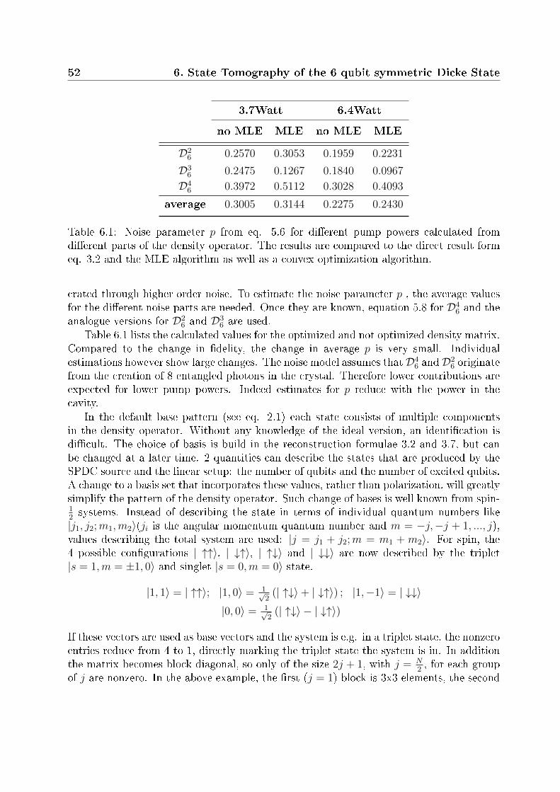
52 6. State Tomography of the 6 qubit symmetric Dicke State

3.7Watt 6.4Watt

no MLE MLE no MLE MLE

D26 0.2570 0.3053 0.1959 0.2231

D36 0.2475 0.1267 0.1840 0.0967

D46 0.3972 0.5112 0.3028 0.4093

average 0.3005 0.3144 0.2275 0.2430

Table 6.1: Noise parameter p from eq. 5.6 for di�erent pump powers calculated fromdi�erent parts of the density operator. The results are compared to the direct result formeq. 3.2 and the MLE algorithm as well as a convex optimization algorithm.

crated through higher order noise. To estimate the noise parameter p , the average valuesfor the di�erent noise parts are needed. Once they are known, equation 5.8 for D4

6 and theanalogue versions for D2

6 and D36 are used.

Table 6.1 lists the calculated values for the optimized and not optimized density matrix.Compared to the change in �delity, the change in average p is very small. Individualestimations however show large changes. The noise model assumes thatD4

6 andD26 originate

from the creation of 8 entangled photons in the crystal. Therefore lower contributions areexpected for lower pump powers. Indeed estimates for p reduce with the power in thecavity.

In the default base pattern (see eq. 2.1) each state consists of multiple componentsin the density operator. Without any knowledge of the ideal version, an identi�cation isdi�cult. The choice of basis is build in the reconstruction formulae 3.2 and 3.7, but canbe changed at a later time. 2 quantities can describe the states that are produced by theSPDC source and the linear setup: the number of qubits and the number of excited qubits.A change to a basis set that incorporates these values, rather than polarization, will greatlysimplify the pattern of the density operator. Such change of bases is well known from spin-12systems. Instead of describing the state in terms of individual quantum numbers like|j1, j2;m1,m2〉(ji is the angular momentum quantum number and m = −j,−j + 1, ..., j),values describing the total system are used: |j = j1 + j2;m = m1 + m2〉. For spin, the4 possible con�gurations | ↑↑〉, | ↓↑〉, | ↑↓〉 and | ↓↓〉 are now described by the triplet|s = 1,m = ±1, 0〉 and singlet |s = 0,m = 0〉 state.

|1, 1〉 = | ↑↑〉; |1, 0〉 = 1√2

(| ↑↓〉+ | ↓↑〉) ; |1,−1〉 = | ↓↓〉|0, 0〉 = 1√

2(| ↑↓〉 − | ↓↑〉)

If these vectors are used as base vectors and the system is e.g. in a triplet state, the nonzeroentries reduce from 4 to 1, directly marking the triplet state the system is in. In additionthe matrix becomes block diagonal, so only of the size 2j + 1, with j = N

2, for each group

of j are nonzero. In the above example, the �rst (j = 1) block is 3x3 elements, the second

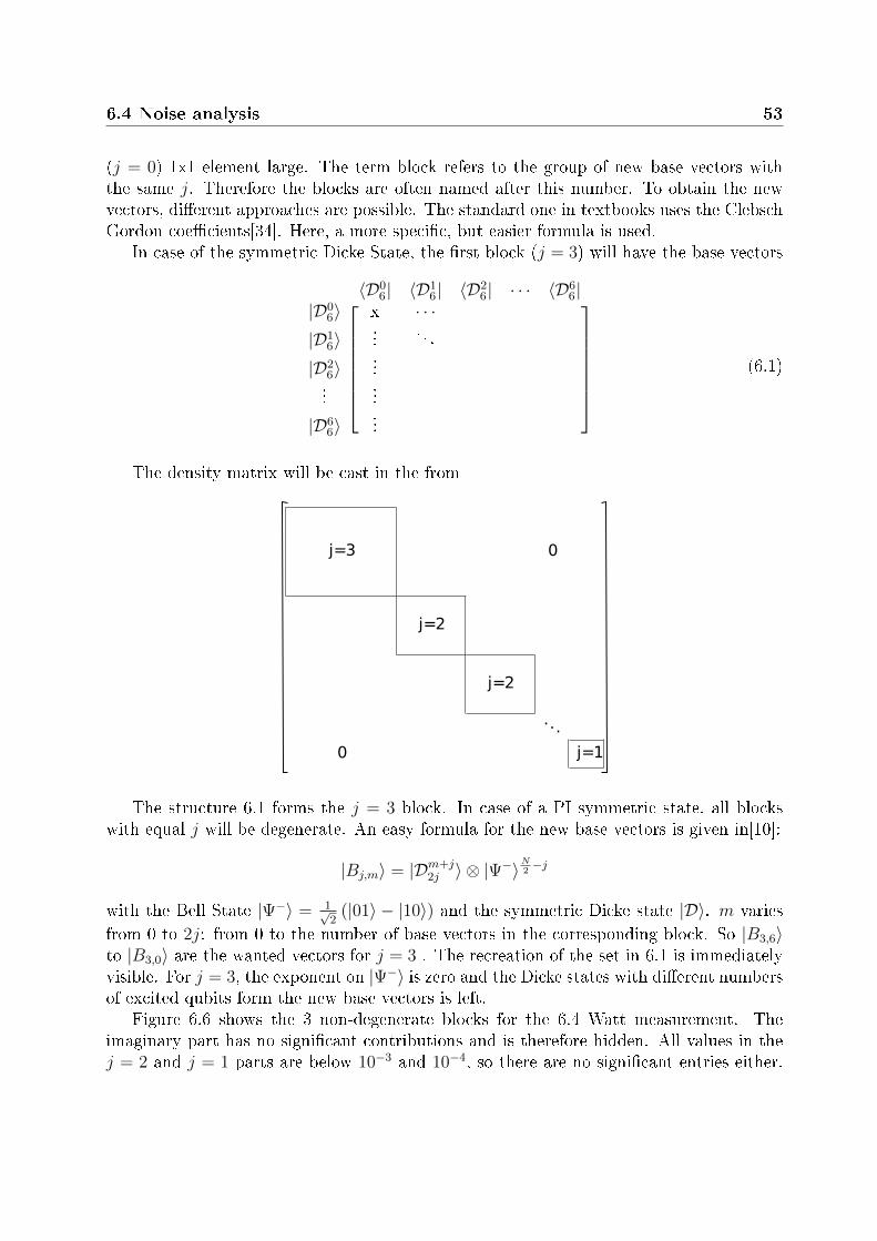
6.4 Noise analysis 53

(j = 0) 1x1 element large. The term block refers to the group of new base vectors withthe same j. Therefore the blocks are often named after this number. To obtain the newvectors, di�erent approaches are possible. The standard one in textbooks uses the ClebschGordon coe�cients[34]. Here, a more speci�c, but easier formula is used.

In case of the symmetric Dicke State, the �rst block (j = 3) will have the base vectors

〈D06| 〈D1

6| 〈D26| · · · 〈D6

6|

|D06〉 x · · ·

|D16〉

.... . .

|D26〉

......

...

|D66〉

...

(6.1)

The density matrix will be cast in the from

j=3 0

j=2

j=2

...

0 j=1

The structure 6.1 forms the j = 3 block. In case of a PI symmetric state, all blockswith equal j will be degenerate. An easy formula for the new base vectors is given in[10]:

|Bj,m〉 = |Dm+j2j 〉 ⊗ |Ψ−〉

N2−j

with the Bell State |Ψ−〉 = 1√2

(|01〉 − |10〉) and the symmetric Dicke state |D〉. m varies

from 0 to 2j: from 0 to the number of base vectors in the corresponding block. So |B3,6〉to |B3,0〉 are the wanted vectors for j = 3 . The recreation of the set in 6.1 is immediatelyvisible. For j = 3, the exponent on |Ψ−〉 is zero and the Dicke states with di�erent numbersof excited qubits form the new base vectors is left.

Figure 6.6 shows the 3 non-degenerate blocks for the 6.4 Watt measurement. Theimaginary part has no signi�cant contributions and is therefore hidden. All values in thej = 2 and j = 1 parts are below 10−3 and 10−4, so there are no signi�cant entries either.

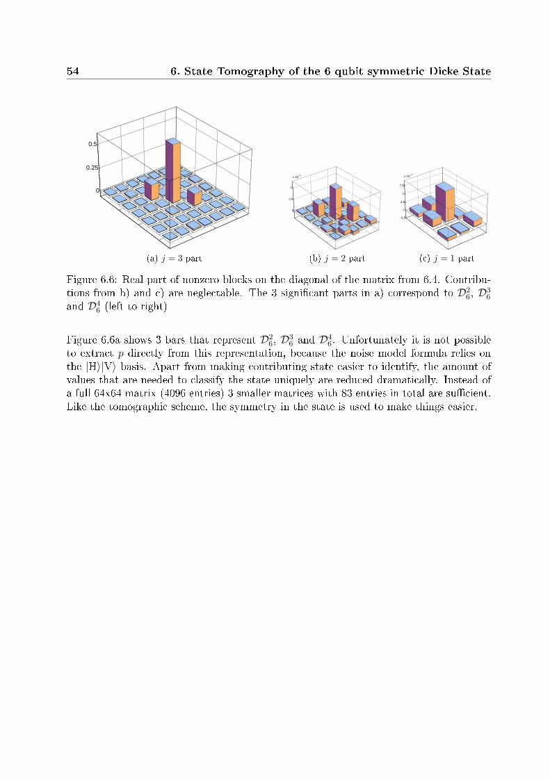
54 6. State Tomography of the 6 qubit symmetric Dicke State

0

0.25

0.5

(a) j = 3 part

0

2.5

5

x 10−3

(b) j = 2 part

−2.5

0

2.5

5

7.5

x 10−4

(c) j = 1 part

Figure 6.6: Real part of nonzero blocks on the diagonal of the matrix from 6.4. Contribu-tions from b) and c) are neglectable. The 3 signi�cant parts in a) correspond to D2

6, D36

and D46 (left to right)

Figure 6.6a shows 3 bars that represent D26, D3

6 and D46. Unfortunately it is not possible

to extract p directly from this representation, because the noise model formula relies onthe |H〉|V〉 basis. Apart from making contributing state easier to identify, the amount ofvalues that are needed to classify the state uniquely are reduced dramatically. Instead ofa full 64x64 matrix (4096 entries) 3 smaller matrices with 83 entries in total are su�cient.Like the tomographic scheme, the symmetry in the state is used to make things easier.

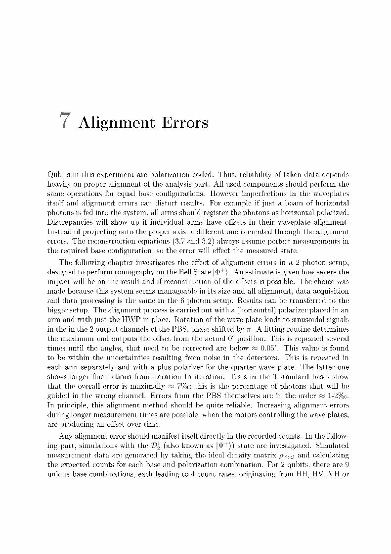
7 Alignment Errors

Qubits in this experiment are polarization coded. Thus, reliability of taken data dependsheavily on proper alignment of the analysis part. All used components should perform thesame operations for equal base con�gurations. However imperfections in the waveplatesitself and alignment errors can distort results. For example if just a beam of horizontalphotons is fed into the system, all arms should register the photons as horizontal polarized.Discrepancies will show up if individual arms have o�sets in their waveplate alignment.Instead of projecting onto the proper axis, a di�erent one is created through the alignmenterrors. The reconstruction equations (3.7 and 3.2) always assume perfect measurements inthe required base con�guration, so the error will e�ect the measured state.

The following chapter investigates the e�ect of alignment errors in a 2 photon setup,designed to perform tomography on the Bell State |Φ+〉. An estimate is given how severe theimpact will be on the result and if reconstruction of the o�sets is possible. The choice wasmade because this system seems manageable in its size and all alignment, data acquisitionand data processing is the same in the 6 photon setup. Results can be transferred to thebigger setup. The alignment process is carried out with a (horizontal) polarizer placed in anarm and with just the HWP in place. Rotation of the wave plate leads to sinusoidal signalsin the in the 2 output channels of the PBS, phase shifted by π. A �tting routine determinesthe maximum and outputs the o�set from the actual 0° position. This is repeated severaltimes until the angles, that need to be corrected are below ≈ 0.05°. This value is foundto be within the uncertainties resulting from noise in the detectors. This is repeated ineach arm separately and with a plus polarizer for the quarter wave plate. The latter oneshows larger �uctuations from iteration to iteration. Tests in the 3 standard bases showthat the overall error is maximally ≈ 7�; this is the percentage of photons that will beguided in the wrong channel. Errors from the PBS themselves are in the order ≈ 1-2�.In principle, this alignment method should be quite reliable. Increasing alignment errorsduring longer measurement times are possible, when the motors controlling the wave plates,are producing an o�set over time.

Any alignment error should manifest itself directly in the recorded counts. In the follow-ing part, simulations with the D1

2 (also known as |Ψ+〉) state are investigated. Simulatedmeasurement data are generated by taking the ideal density matrix ρideal and calculatingthe expected counts for each base and polarization combination. For 2 qubits, there are 9unique base combinations, each leading to 4 count rates, originating from HH, HV, VH or

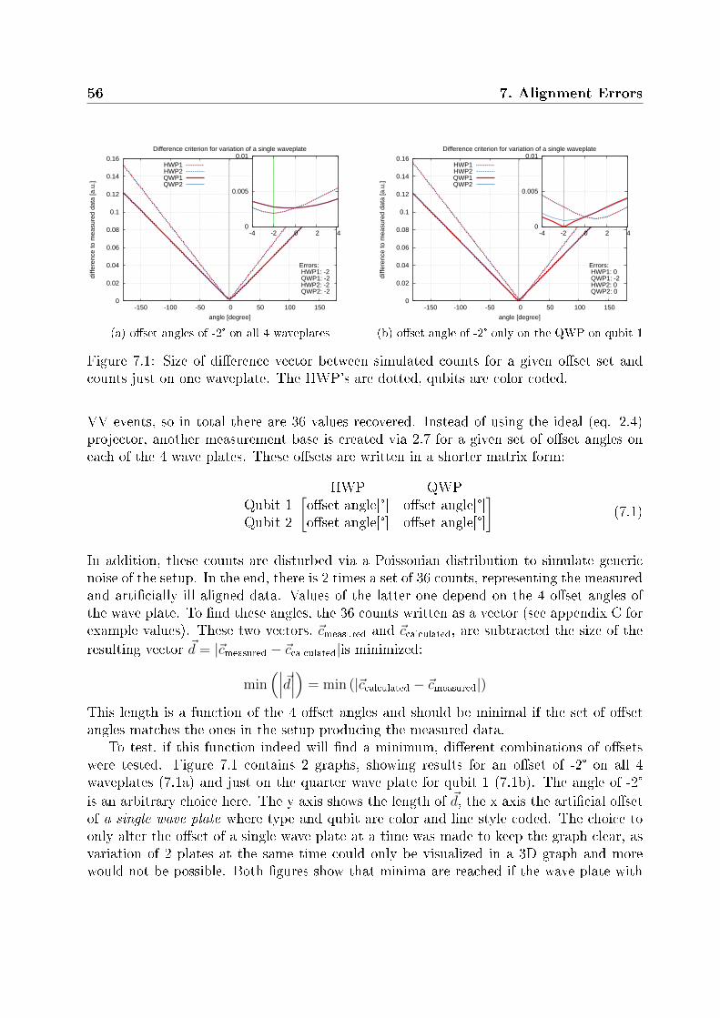
56 7. Alignment Errors

0

0.02

0.04

0.06

0.08

0.1

0.12

0.14

0.16

-150 -100 -50 0 50 100 150

diffe

renc

e to

mea

sure

d da

ta [a

.u.]

angle [degree]

Difference criterion for variation of a single waveplate

HWP1HWP2QWP1QWP2

0

0.005

0.01

-4 -2 0 2 4

Errors: HWP1: -2 QWP1: -2 HWP2: -2 QWP2: -2

(a) o�set angles of -2° on all 4 waveplates

0

0.02

0.04

0.06

0.08

0.1

0.12

0.14

0.16

-150 -100 -50 0 50 100 150

diffe

renc

e to

mea

sure

d da

ta [a

.u.]

angle [degree]

Difference criterion for variation of a single waveplate

HWP1HWP2QWP1QWP2

0

0.005

0.01

-4 -2 0 2 4

Errors: HWP1: 0 QWP1: -2 HWP2: 0 QWP2: 0

(b) o�set angle of -2° only on the QWP on qubit 1

Figure 7.1: Size of di�erence vector between simulated counts for a given o�set set andcounts just on one waveplate. The HWP's are dotted, qubits are color coded.

VV events, so in total there are 36 values recovered. Instead of using the ideal (eq. 2.4)projector, another measurement base is created via 2.7 for a given set of o�set angles oneach of the 4 wave plates. These o�sets are written in a shorter matrix form:

HWP QWP[ ]Qubit 1 o�set angle[°] o�set angle[°]Qubit 2 o�set angle[°] o�set angle[°]

(7.1)

In addition, these counts are disturbed via a Poissonian distribution to simulate genericnoise of the setup. In the end, there is 2 times a set of 36 counts, representing the measuredand arti�cially ill aligned data. Values of the latter one depend on the 4 o�set angles ofthe wave plate. To �nd these angles, the 36 counts written as a vector (see appendix C forexample values). These two vectors, ~cmeasured and ~ccalculated, are subtracted the size of the

resulting vector ~d = |~cmeasured − ~ccalculated|is minimized:

min(∣∣∣~d∣∣∣) = min (|~ccalculated − ~cmeasured|)

This length is a function of the 4 o�set angles and should be minimal if the set of o�setangles matches the ones in the setup producing the measured data.

To test, if this function indeed will �nd a minimum, di�erent combinations of o�setswere tested. Figure 7.1 contains 2 graphs, showing results for an o�set of -2° on all 4waveplates (7.1a) and just on the quarter wave plate for qubit 1 (7.1b). The angle of -2°

is an arbitrary choice here. The y axis shows the length of ~d, the x axis the arti�cial o�setof a single wave plate where type and qubit are color and line style coded. The choice toonly alter the o�set of a single wave plate at a time was made to keep the graph clear, asvariation of 2 plates at the same time could only be visualized in a 3D graph and morewould not be possible. Both �gures show that minima are reached if the wave plate with

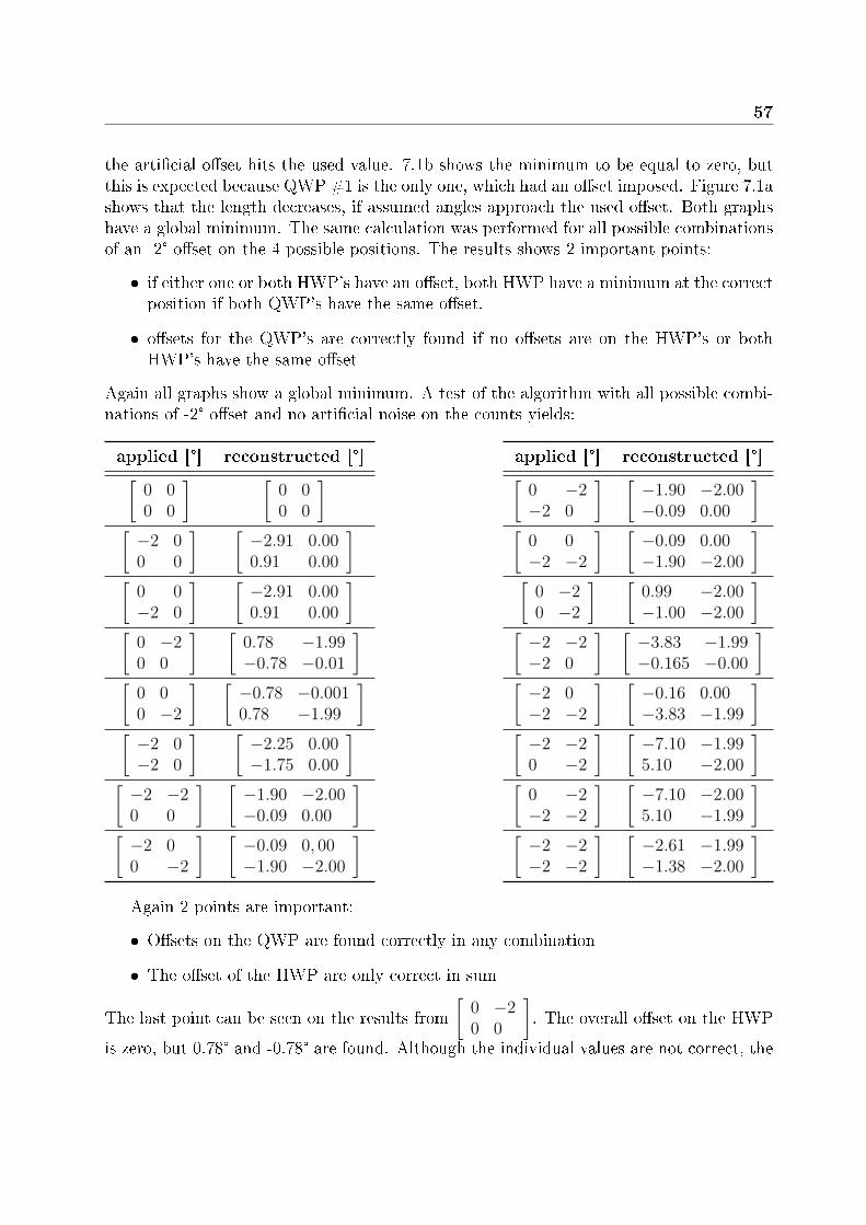
57

the arti�cial o�set hits the used value. 7.1b shows the minimum to be equal to zero, butthis is expected because QWP #1 is the only one, which had an o�set imposed. Figure 7.1ashows that the length decreases, if assumed angles approach the used o�set. Both graphshave a global minimum. The same calculation was performed for all possible combinationsof an -2° o�set on the 4 possible positions. The results shows 2 important points:

� if either one or both HWP's have an o�set, both HWP have a minimum at the correctposition if both QWP's have the same o�set.

� o�sets for the QWP's are correctly found if no o�sets are on the HWP's or bothHWP's have the same o�set

Again all graphs show a global minimum. A test of the algorithm with all possible combi-nations of -2° o�set and no arti�cial noise on the counts yields:

applied [°] reconstructed [°][0 00 0

] [0 00 0

][−2 00 0

] [−2.91 0.000.91 0.00

][

0 0−2 0

] [−2.91 0.000.91 0.00

][

0 −20 0

] [0.78 −1.99−0.78 −0.01

][

0 00 −2

] [−0.78 −0.0010.78 −1.99

][−2 0−2 0

] [−2.25 0.00−1.75 0.00

][−2 −20 0

] [−1.90 −2.00−0.09 0.00

][−2 00 −2

] [−0.09 0, 00−1.90 −2.00

]

applied [°] reconstructed [°][0 −2−2 0

] [−1.90 −2.00−0.09 0.00

][

0 0−2 −2

] [−0.09 0.00−1.90 −2.00

][

0 −20 −2

] [0.99 −2.00−1.00 −2.00

][−2 −2−2 0

] [−3.83 −1.99−0.165 −0.00

][−2 0−2 −2

] [−0.16 0.00−3.83 −1.99

][−2 −20 −2

] [−7.10 −1.995.10 −2.00

][

0 −2−2 −2

] [−7.10 −2.005.10 −1.99

][−2 −2−2 −2

] [−2.61 −1.99−1.38 −2.00

]Again 2 points are important:

� O�sets on the QWP are found correctly in any combination

� The o�set of the HWP are only correct in sum

The last point can be seen on the results from

[0 −20 0

]. The overall o�set on the HWP

is zero, but 0.78° and -0.78° are found. Although the individual values are not correct, the

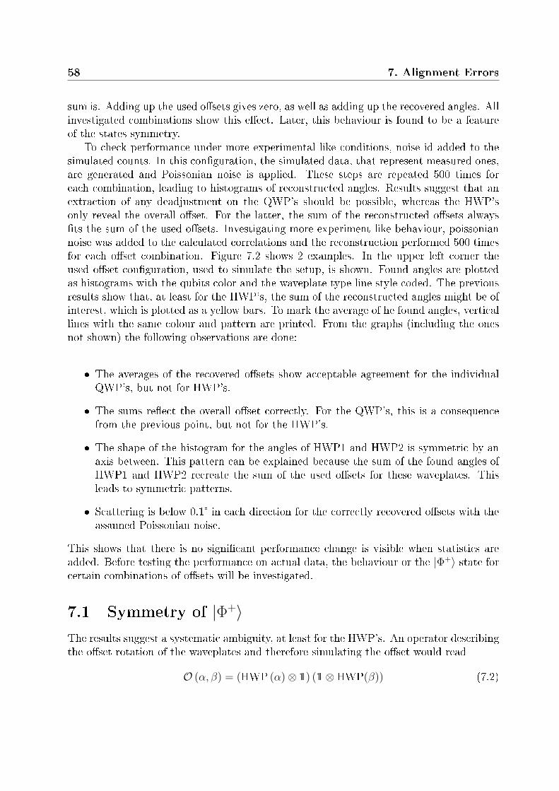
58 7. Alignment Errors

sum is. Adding up the used o�sets gives zero, as well as adding up the recovered angles. Allinvestigated combinations show this e�ect. Later, this behaviour is found to be a featureof the states symmetry.

To check performance under more experimental like conditions, noise id added to thesimulated counts. In this con�guration, the simulated data, that represent measured ones,are generated and Poissonian noise is applied. These steps are repeated 500 times foreach combination, leading to histograms of reconstructed angles. Results suggest that anextraction of any deadjustment on the QWP's should be possible, whereas the HWP'sonly reveal the overall o�set. For the latter, the sum of the reconstructed o�sets always�ts the sum of the used o�sets. Investigating more experiment like behaviour, poissoniannoise was added to the calculated correlations and the reconstruction performed 500 timesfor each o�set combination. Figure 7.2 shows 2 examples. In the upper left corner theused o�set con�guration, used to simulate the setup, is shown. Found angles are plottedas histograms with the qubits color and the waveplate type line style coded. The previousresults show that, at least for the HWP's, the sum of the reconstructed angles might be ofinterest, which is plotted as a yellow bars. To mark the average of he found angles, verticallines with the same colour and pattern are printed. From the graphs (including the onesnot shown) the following observations are done:

� The averages of the recovered o�sets show acceptable agreement for the individualQWP's, but not for HWP's.

� The sums re�ect the overall o�set correctly. For the QWP's, this is a consequencefrom the previous point, but not for the HWP's.

� The shape of the histogram for the angles of HWP1 and HWP2 is symmetric by anaxis between. This pattern can be explained because the sum of the found angles ofHWP1 and HWP2 recreate the sum of the used o�sets for these waveplates. Thisleads to symmetric patterns.

� Scattering is below 0.1° in each direction for the correctly recovered o�sets with theassumed Poissonian noise.

This shows that there is no signi�cant performance change is visible when statistics areadded. Before testing the performance on actual data, the behaviour or the |Φ+〉 state forcertain combinations of o�sets will be investigated.

7.1 Symmetry of |Φ+〉The results suggest a systematic ambiguity, at least for the HWP's. An operator describingthe o�set rotation of the waveplates and therefore simulating the o�set would read

O (α, β) = (HWP (α)⊗ 1) (1⊗ HWP(β)) (7.2)

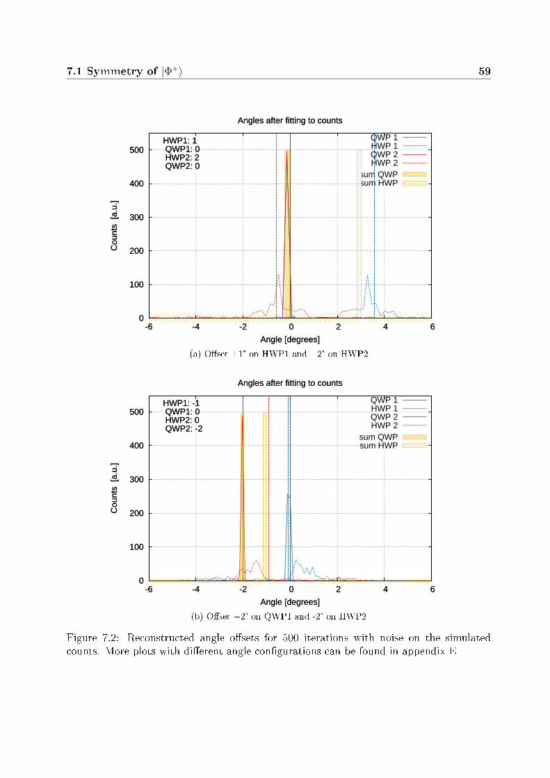
7.1 Symmetry of |Φ+〉 59

0

100

200

300

400

500

-6 -4 -2 0 2 4 6

Cou

nts

[a.u

.]

Angle [degrees]

Angles after fitting to counts

HWP1: 1 QWP1: 0 HWP2: 2 QWP2: 0

sum QWPsum HWP

0

100

200

300

400

500

-6 -4 -2 0 2 4 6

Cou

nts

[a.u

.]

Angle [degrees]

Angles after fitting to counts

HWP1: 1 QWP1: 0 HWP2: 2 QWP2: 0

QWP 1HWP 1QWP 2HWP 2

(a) O�set +1° on HWP1 and +2° on HWP2

0

100

200

300

400

500

-6 -4 -2 0 2 4 6

Cou

nts

[a.u

.]

Angle [degrees]

Angles after fitting to counts

HWP1: -1 QWP1: 0 HWP2: 0 QWP2: -2

sum QWPsum HWP

0

100

200

300

400

500

-6 -4 -2 0 2 4 6

Cou

nts

[a.u

.]

Angle [degrees]

Angles after fitting to counts

HWP1: -1 QWP1: 0 HWP2: 0 QWP2: -2

QWP 1HWP 1QWP 2HWP 2

(b) O�set +2° on QWP1 and -2° on HWP2

Figure 7.2: Reconstructed angle o�sets for 500 iterations with noise on the simulatedcounts. More plots with di�erent angle con�gurations can be found in appendix E

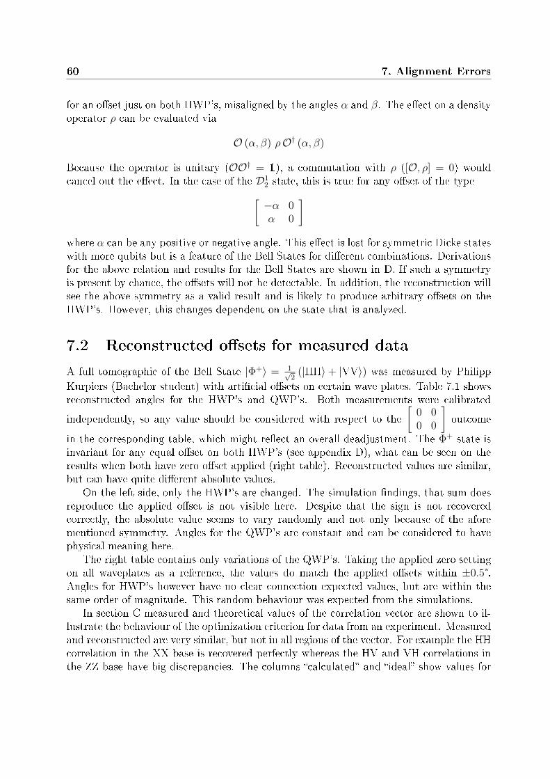
60 7. Alignment Errors

for an o�set just on both HWP's, misaligned by the angles α and β. The e�ect on a densityoperator ρ can be evaluated via

O (α, β) ρO† (α, β)

Because the operator is unitary (OO† = 1), a commutation with ρ ([O, ρ] = 0) wouldcancel out the e�ect. In the case of the D1

2 state, this is true for any o�set of the type[−α 0α 0

]where α can be any positive or negative angle. This e�ect is lost for symmetric Dicke stateswith more qubits but is a feature of the Bell States for di�erent combinations. Derivationsfor the above relation and results for the Bell States are shown in D. If such a symmetryis present by chance, the o�sets will not be detectable. In addition, the reconstruction willsee the above symmetry as a valid result and is likely to produce arbitrary o�sets on theHWP's. However, this changes dependent on the state that is analyzed.

7.2 Reconstructed o�sets for measured data

A full tomographic of the Bell State |Φ+〉 = 1√2

(|HH〉+ |VV〉) was measured by Philipp

Kurpiers (Bachelor student) with arti�cial o�sets on certain wave plates. Table 7.1 showsreconstructed angles for the HWP's and QWP's. Both measurements were calibrated

independently, so any value should be considered with respect to the

[0 00 0

]outcome

in the corresponding table, which might re�ect an overall deadjustment. The Φ+ state isinvariant for any equal o�set on both HWP's (see appendix D), what can be seen on theresults when both have zero o�set applied (right table). Reconstructed values are similar,but can have quite di�erent absolute values.

On the left side, only the HWP's are changed. The simulation �ndings, that sum doesreproduce the applied o�set is not visible here. Despite that the sign is not recoveredcorrectly, the absolute value seems to vary randomly and not only because of the aforementioned symmetry. Angles for the QWP's are constant and can be considered to havephysical meaning here.

The right table contains only variations of the QWP's. Taking the applied zero settingon all waveplates as a reference, the values do match the applied o�sets within ±0.5°.Angles for HWP's however have no clear connection expected values, but are within thesame order of magnitude. This random behaviour was expected from the simulations.

In section C measured and theoretical values of the correlation vector are shown to il-lustrate the behaviour of the optimization criterion for data from an experiment. Measuredand reconstructed are very similar, but not in all regions of the vector. For example the HHcorrelation in the XX base is recovered perfectly whereas the HV and VH correlations inthe ZZ base have big discrepancies. The columns �calculated� and �ideal� show values for

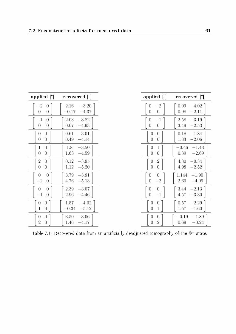
7.2 Reconstructed o�sets for measured data 61

applied [°] recovered [°][−2 00 0

] [2.16 −3.20−0.17 −4.37

][−1 00 0

] [2.03 −3.820.07 −4.93

][

0 00 0

] [0.61 −3.010.49 −4.14

][

1 00 0

] [1.8 −3.501.63 −4.59

][

2 00 0

] [0.12 −3.951.12 −5.20

][

0 0−2 0

] [3.79 −3.914.76 −5.13

][

0 0−1 0

] [2.39 −3.072.96 −4.46

][

0 01 0

] [1.57 −4.02−0.34 −5.12

][

0 02 0

] [3.50 −3.061.46 −4.17

]

applied [°] recovered [°][0 −20 0

] [0.09 −4.020.98 −2.11

][

0 −10 0

] [2.58 −3.193.49 −2.53

][

0 00 0

] [0.18 −1.841.33 −2.06

][

0 10 0

] [−0.46 −1.430.39 −2.69

][

0 20 0

] [4.30 −0.344.98 −2.52

][

0 00 −2

] [1.144 −1.902.60 −4.09

][

0 00 −1

] [3.44 −2.134.57 −3.30

][

0 00 1

] [0.57 −2.291.57 −1.60

][

0 00 2

] [−0.19 −1.890.69 −0.24

]Table 7.1: Recovered data from an arti�cially deadjusted tomography of the Φ+ state.

62 7. Alignment Errors

the ideal o�set just on a single waveplate and of the ideal state without any perturbation.In comparison, only a few entries di�er, the majority is the same. This is expected, becausean o�set on any HWP will just alter any results measured in the X basis. This featurecould be exploited in a di�erent optimization result where only parts of the correlationvector are investigated that actually would change for the considered waveplates.

7.3 E�ects on Eigenvalues and Fidelity

O�sets on di�erent waveplates lead to di�erent behaviour of the eigenvalues and �delities.

The smallest eigenvalue (−0.0726) was found for the combination

[0 −20 −2

]. The numeric

value depends on the value (it will increase for bigger o�sets) but this pattern immediatelyproduces large negative eigenvalues. Alignment errors only on the HWP's result in eigen-values in the order of −1 · 10−16 what can be considered to be in machine precision ando�sets on HWP's and QWP's simultaneously produces values in the order of −1 · 10−2, soroughly an order in magnitude less than the above.

Fidelity on the other hand does severely depend on the HWP's. The smallest ones were

found for

[α 0α 0

]type patterns (roughly 98% for a = ±2°). If the state is a mixture,

typical �delities are in the order of ≈ 60% for a mixture of D12, D0

2 and D22. This shows

that general statements on sources for low �delity or the occurrence of negative eigenvalueshare hard to be made, especially for larger systems where more combinations are possible.

7.4 Summary

Results in this chapter can be seen as a starting point to develop more sophisticated meth-ods for �nding alignment errors of wave plates. The used method relies on the knowledgeof the real state, but this is not a good ansatz, as the calculated o�sets will �t the expectedcounts. This is forced by the algorithm, but there is no guarantee for a connection to thereal state that was measured in the setup. For example the wave plates could adapt toother alignment errors. If the 2 emission cones of the SPDC are coupled into the �ber witha di�erent ratio, the counts will shift as well. An ideal scheme should be independent onknowledge of the state.

During alignment, the wave plates should be balanced relative to each other, that thesame data will be measured for the same polarization state. In case of the 6 photonic linearsetup from chapter 5.3, not only 6fold but any lower number is recorded. These eventscould be used to develop a scheme that allows an alignment of the wave plate relative toeach other. This way, an overall o�set cannot be excluded de�nitely, but such an alignmenterror will result in a global rotation of the state and this is quite easy to detect.

8 Conclusion and Outlook

In conclusion it was shown that exploiting symmetries in states can be used to reducethe e�ort to 3.8% compared to the generic tomographic scheme. This allowed the inves-tigation of a 6 photonic state that would be inaccessible through the standard approach.Information about noise was preserved in the measurement and supported the expectednoise model. The symmetric Dicke State was produced and observed with high accuracywhile demonstrating the power of permutationally invariant quantum state tomography.Although the scheme is kept as general as possible, only a subspace of all possible densitymatrices is accessible; the space which ful�lls the symmetry requirement.

If the observed state lies in this subspace, the scheme is equivalent to generic tomog-raphy. Another approach uses a method known as compressed sensing[19] for state to-mography. This technique is originally known from signal processing and allows the guessof a signal from a certain amount of information. In state tomography, the informationcorresponds to local measurement settings. The expected number of sets that are neededfor reliable estimation is in the same order as for permutationally invariant tomography,although slightly higher. Another bene�t is that the reconstruction of the density operatoralready includes optimization routines. They make use of convex optimization[33] and willtherefore reach the global optimum.

In the last chapter, the e�ect of o�set in the wave plate rotations due to alignmenterrors is investigated. For the used 2 qubit examples, consistent results could be achieved.Performance and behaviour depends on symmetries of the observed state, because o�setscan cancel out for special sign combinations. Starting with these �ndings, a method toinvestigate the linear optic setup used for 6 qubit tomography could be developed. Insteadof relying on the knowledge of the ideal state, a relative scheme should be possible. Relativemeans that analysis blocks show o�sets relative to each other rather than absolute ones toan assumed state.

64 8. Conclusion and Outlook

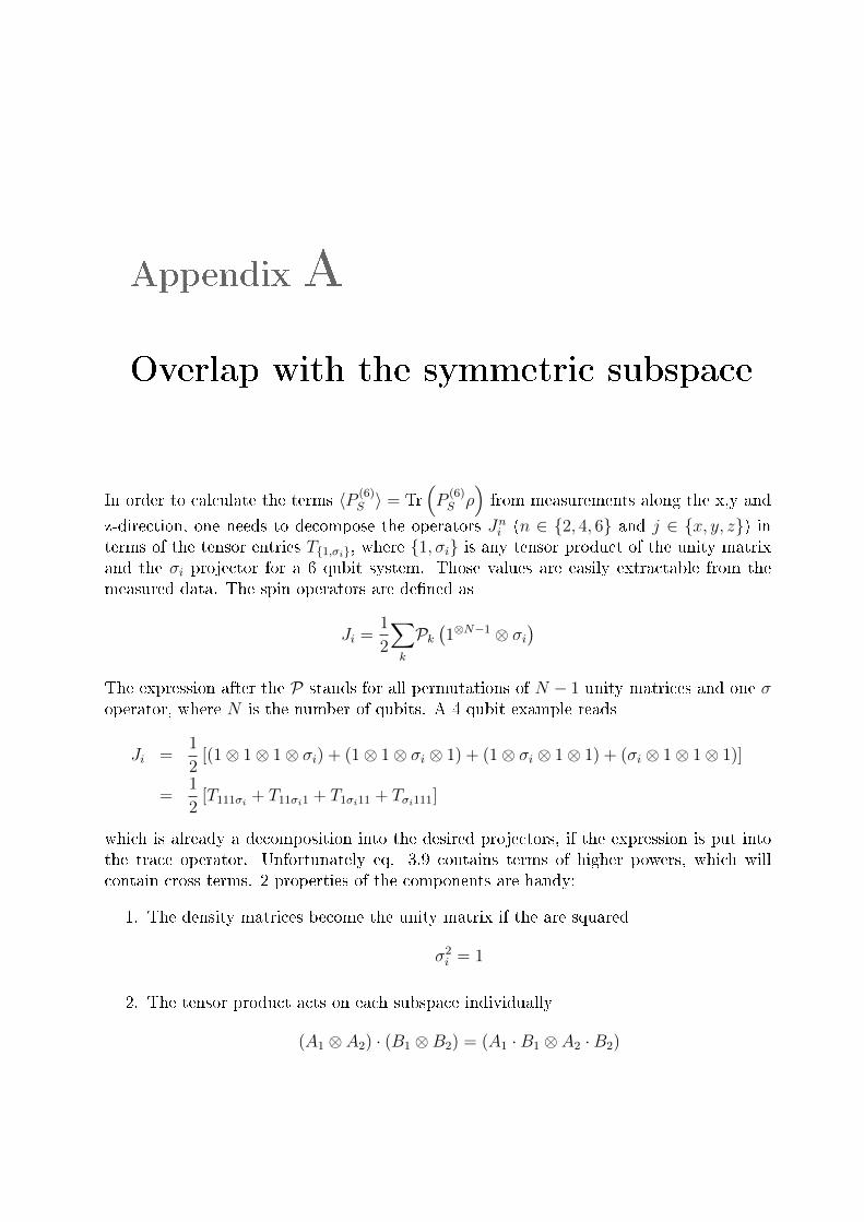
Appendix A

Overlap with the symmetric subspace

In order to calculate the terms 〈P (6)S 〉 = Tr

(P

(6)S ρ

)from measurements along the x,y and

z-direction, one needs to decompose the operators Jni (n ∈ {2, 4, 6} and j ∈ {x, y, z}) interms of the tensor entries T{1,σi}, where {1, σi} is any tensor product of the unity matrixand the σi projector for a 6 qubit system. Those values are easily extractable from themeasured data. The spin operators are de�ned as

Ji =1

2

∑k

Pk(1⊗N−1 ⊗ σi

)The expression after the P stands for all permutations of N − 1 unity matrices and one σoperator, where N is the number of qubits. A 4 qubit example reads

Ji =1

2[(1⊗ 1⊗ 1⊗ σi) + (1⊗ 1⊗ σi ⊗ 1) + (1⊗ σi ⊗ 1⊗ 1) + (σi ⊗ 1⊗ 1⊗ 1)]

=1

2[T111σi + T11σi1 + T1σi11 + Tσi111]

which is already a decomposition into the desired projectors, if the expression is put intothe trace operator. Unfortunately eq. 3.9 contains terms of higher powers, which willcontain cross terms. 2 properties of the components are handy:

1. The density matrices become the unity matrix if the are squared

σ2i = 1

2. The tensor product acts on each subspace individually

(A1 ⊗ A2) · (B1 ⊗B2) = (A1 ·B1 ⊗ A2 ·B2)

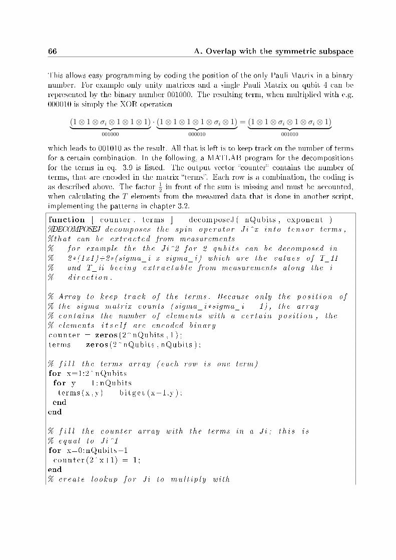
66 A. Overlap with the symmetric subspace

This allows easy programming by coding the position of the only Pauli Matrix in a binarynumber. For example only unity matrices and a single Pauli Matrix on qubit 4 can berepresented by the binary number 001000. The resulting term, when multiplied with e.g.000010 is simply the XOR operation

(1⊗ 1⊗ σi ⊗ 1⊗ 1⊗ 1)︸ ︷︷ ︸001000

· (1⊗ 1⊗ 1⊗ 1⊗ σi ⊗ 1)︸ ︷︷ ︸000010

= (1⊗ 1⊗ σi ⊗ 1⊗ σi ⊗ 1)︸ ︷︷ ︸001010

which leads to 001010 as the result. All that is left is to keep track on the number of termsfor a certain combination. In the following, a MATLAB program for the decompositionsfor the terms in eq. 3.9 is listed. The output vector �counter� contains the number ofterms, that are encoded in the matrix �terms�. Each row is a combination, the coding isas described above. The factor 1

2in front of the sum is missing and must be accounted,

when calculating the T elements from the measured data that is done in another script,implementing the patterns in chapter 3.2.

function [ counter , terms ] = decomposeJ ( nQubits , exponent )%DECOMPOSEJ decomposes the sp in opera tor J i^x in t o t ensor terms ,%tha t can be e x t r a c t e d from measurements% fo r example the the J i^2 f o r 2 q u b i t s can be decomposed in% 2*(1 x1 )+2*( sigma_i x sigma_i ) which are the va l u e s o f T_11% and T_ii bee ing e x t r a c t a b l e from measurements a long the i% d i r e c t i o n .

% Array to keep t rack o f the terms . Because on ly the p o s i t i o n o f% the sigma matrix counts ( sigma_i* sigma_i = 1) , the array% conta ins the number o f e lements wi th a c e r t a i n pos i t i on , the% elements i t s e l f are encoded b inarycounter = zeros (2^nQubits , 1 ) ;terms = zeros (2^nQubits , nQubits ) ;

% f i l l t he terms array ( each row i s one term )for x=1:2^nQubitsfor y = 1 : nQubitsterms (x , y ) = b i t g e t (x−1,y ) ;

endend

% f i l l t he counter array wi th the terms in a Ji ; t h i s i s% equa l to J i^1for x=0:nQubits−1counter (2^x+1) = 1 ;

end% crea t e lookup f o r J i to mu l t i p l y wi th

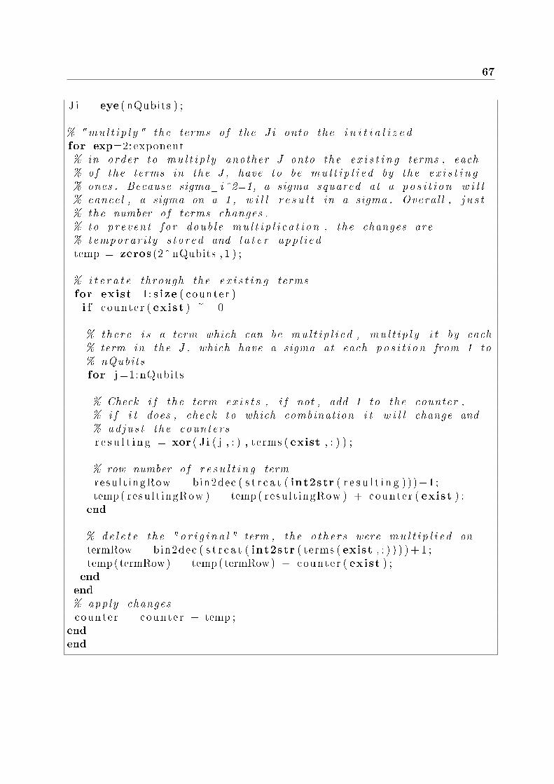
67

J i = eye ( nQubits ) ;

% "mu l t i p l y " the terms o f the J i onto the i n i t i a l i z e dfor exp=2: exponent% in order to mu l t i p l y another J onto the e x i s t i n g terms , each% of the terms in the J , have to be mu l t i p l i e d by the e x i s t i n g% ones . Because sigma_i^2=1, a sigma squared at a p o s i t i o n w i l l% cance l , a sigma on a 1 , w i l l r e s u l t in a sigma . Overa l l , j u s t% the number o f terms changes .% to prevent f o r doub le mu l t i p l i c a t i o n , the changes are% temporar i l y s t o r ed and l a t e r app l i e dtemp = zeros (2^nQubits , 1 ) ;

% i t e r a t e through the e x i s t i n g termsfor exist=1: s ize ( counter )i f counter ( exist ) ~= 0

% there i s a term which can be mu l t i p l i e d , mu l t i p l y i t by each% term in the J , which have a sigma at each po s i t i o n from 1 to% nQubitsfor j =1: nQubits

% Check i f the term e x i s t s , i f not , add 1 to the counter ,% i f i t does , check to which combination i t w i l l change and% ad ju s t the countersr e s u l t i n g = xor ( J i ( j , : ) , terms ( exist , : ) ) ;

% row number o f r e s u l t i n g termresult ingRow = bin2dec ( s t r c a t ( int2str ( r e s u l t i n g ) ) )+1 ;temp( result ingRow ) = temp( result ingRow ) + counter ( exist ) ;end

% de l e t e the " o r i g i n a l " term , the o the r s were mu l t i p l i e d ontermRow = bin2dec ( s t r c a t ( int2str ( terms ( exist , : ) ) ) )+ 1 ;temp(termRow) = temp(termRow) − counter ( exist ) ;endend% app ly changescounter = counter + temp ;

endend

68 A. Overlap with the symmetric subspace

Appendix B

Density matrix contributions

To develop an idea how full tomography and PI tomography build up the density matrix, itis helpful to have a look at the number of elements that are summed up or subtracted at thedi�erent entries. Especially to gauge the impact of measurement errors this informationis useful because elements with more contributions are likely to have smaller errors thanones with less ones. A color plot is shown in �gure B.1. The statistics give

Full Tomography PI Tomography

Minimum 64 4

Maximum 64 63

Average 64 11.75

As expected, PI Tomography has less contributions per matrix element and insteadof a homogeneous distribution patterns are visible. To develop an understanding of theerror,it is not only useful to know the number of contributors, but how values are added orsubtracted. If the same value is added and subtracted again that they drop out, the errorbecomes large.

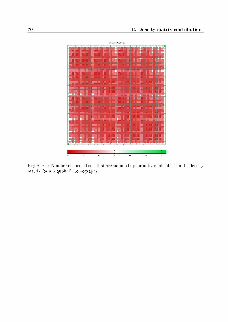
70 B. Density matrix contributions

Figure B.1: Number of correlations that are summed up for individual entries in the densitymatrix for a 6 qubit PI tomography.

Appendix C

Counts for |Ψ+〉 = 1√2

(|HH〉 + |VV〉)

In Chapter 7 results from a 2 qubit tomography are used to extract possible o�set an-gles for the waveplates, but do not lead to reasonable results. Here, the measured and

theoretical correlations are shown. The calculated values assume an error of

[−2 00 0

]what should correspond to the physical error as well; the reconstruction algorithm outputs[

2.16 −3.20−0.17 −4.37

]which are used in the �reconstructed� column. Ideal is a |Ψ+〉 state

without any error. Measured correlations are not away from the calculated, but the dis-tance between calculated and ideal is surprisingly low. The �ne discrepancies in only afew entries is absorbed by the statistical �uctuations. On the other side, entries in thereconstructed column are somewhere between measured and calculated. Distance to mea-sured and calculated values seems low. It is important to note that for the 0° o�set on all

waveplates the con�guration

[0.61 −3.010.49 −4.14

]was found, what might explain the angles of

the quarter wave plates as a global error in addition to the arti�cial created.

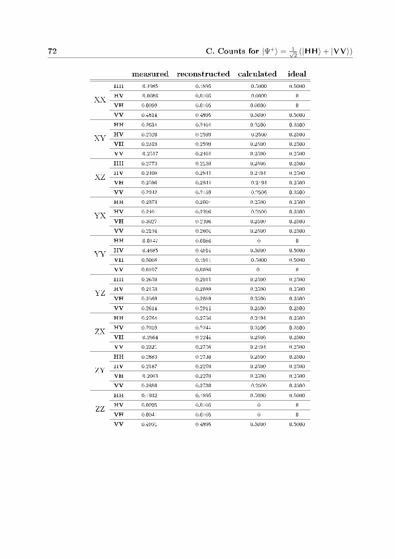
72 C. Counts for |Ψ+〉 = 1√2

(|HH〉+ |VV〉)

measured reconstructed calculated ideal

HH 0.4985 0.4895 0.5000 0.5000

XXHV 0.0086 0.0105 0.0000 0

VH 0.0099 0.0105 0.0000 0

VV 0.4814 0.4895 0.5000 0.5000

HH 0.2634 0.2401 0.2500 0.2500

XYHV 0.2520 0.2599 0.2500 0.2500

VH 0.2319 0.2599 0.2500 0.2500

VV 0.2517 0.2401 0.2500 0.2500

HH 0.2773 0.2159 0.2506 0.2500

XZHV 0.2400 0.2841 0.2494 0.2500

VH 0.2596 0.2841 0.2494 0.2500

VV 0.2242 0.2159 0.2506 0.2500

HH 0.2373 0.2604 0.2500 0.2500

YXHV 0.2401 0.2396 0.2500 0.2500

VH 0.3027 0.2396 0.2500 0.2500

VV 0.2194 0.2604 0.2500 0.2500

HH 0.0147 0.0086 0 0

YYHV 0.4685 0.4914 0.5000 0.5000

VH 0.5066 0.4914 0.5000 0.5000

VV 0.0107 0.0086 0 0

HH 0.2659 0.2911 0.2500 0.2500

YZHV 0.2153 0.2089 0.2500 0.2500

VH 0.2569 0.2089 0.2500 0.2500

VV 0.2614 0.2911 0.2500 0.2500

HH 0.2764 0.2756 0.2494 0.2500

ZXHV 0.2259 0.2244 0.2506 0.2500

VH 0.2664 0.2244 0.2506 0.2500

VV 0.2321 0.2756 0.2494 0.2500

HH 0.2883 0.2730 0.2500 0.2500

ZYHV 0.2187 0.2270 0.2500 0.2500

VH 0.2063 0.2270 0.2500 0.2500

VV 0.2880 0.2730 0.2500 0.2500

HH 0.4932 0.4895 0.5000 0.5000

ZZHV 0.0025 0.0105 0 0

VH 0.0041 0.0105 0 0

VV 0.4991 0.4895 0.5000 0.5000

Appendix D

Symmetries

In chapter 7, it was found that symmetric errors in the position of the HWP's and QWPcan cancel out.

D.1 The 2 qubit symmetric Dicke State

The results from the simulations suggest that errors on the HWP's on qubit 1 and 2 cancancel out. The density matrix for D1

2 reads

|D12〉 =

1√2

(|HV〉+ |VH〉)⇒ ρD12

=1

2

0 0 0 00 1 1 00 1 1 00 0 0 0

Rotations of the state by the 2 HWP's is done via the operator

O (α, β) = HWP (α)⊗ HWP (β)

for the operations to cancel

O (α, β) ρD12O (α, β)† = ρD1

2

must hold. With γ = 2α + 2β

O (α, β) ρD12O (α, β)† =

1

2

sin (γ)2 − sin (γ) cos (γ) − sin (γ) cos (γ) − sin (γ)2

− sin (γ) cos (γ) cos (γ)2 cos (γ)2 cos (γ) sin (γ)

− sin (γ) cos (γ) cos (γ)2 cos (γ)2 cos (γ) sin (γ)

− sin (γ)2 cos (γ) sin (γ) cos (γ) sin (γ) sin (γ)2

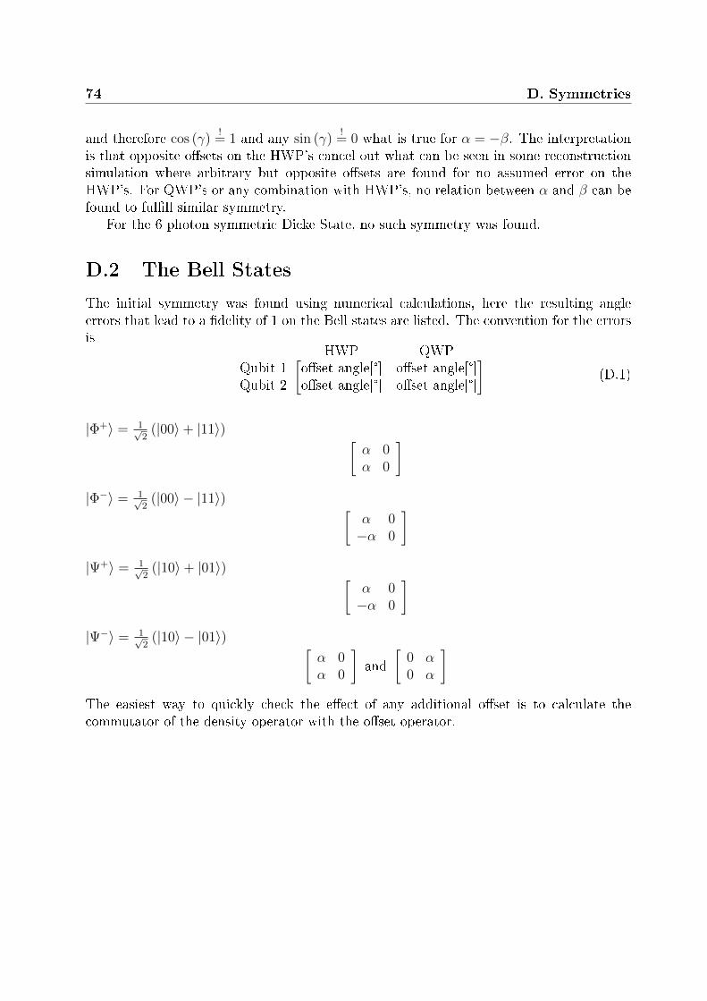
74 D. Symmetries

and therefore cos (γ)!

= 1 and any sin (γ)!

= 0 what is true for α = −β. The interpretationis that opposite o�sets on the HWP's cancel out what can be seen in some reconstructionsimulation where arbitrary but opposite o�sets are found for no assumed error on theHWP's. For QWP's or any combination with HWP's, no relation between α and β can befound to ful�ll similar symmetry.

For the 6 photon symmetric Dicke State, no such symmetry was found.

D.2 The Bell States

The initial symmetry was found using numerical calculations, here the resulting angleerrors that lead to a �delity of 1 on the Bell states are listed. The convention for the errorsis

HWP QWP[ ]Qubit 1 o�set angle[°] o�set angle[°]Qubit 2 o�set angle[°] o�set angle[°]

(D.1)

|Φ+〉 = 1√2

(|00〉+ |11〉) [α 0α 0

]|Φ−〉 = 1√

2(|00〉 − |11〉) [

α 0−α 0

]|Ψ+〉 = 1√

2(|10〉+ |01〉) [

α 0−α 0

]|Ψ−〉 = 1√

2(|10〉 − |01〉) [

α 0α 0

]and

[0 α0 α

]The easiest way to quickly check the e�ect of any additional o�set is to calculate thecommutator of the density operator with the o�set operator.

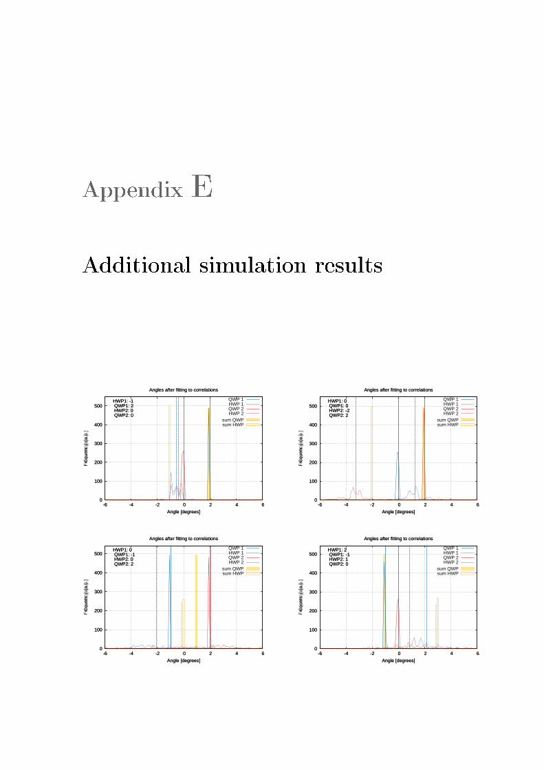
Appendix E

Additional simulation results

0

100

200

300

400

500

-6 -4 -2 0 2 4 6

Cou

nts

[a.u

.]

Angle [degrees]

Angles after fitting to correlations

HWP1: -1 QWP1: 2 HWP2: 0 QWP2: 0

sum QWPsum HWP

0

100

200

300

400

500

-6 -4 -2 0 2 4 6

Fre

quen

cy [

a.u.

]

Angle [degrees]

Angles after fitting to correlations

HWP1: -1 QWP1: 2 HWP2: 0 QWP2: 0

QWP 1HWP 1QWP 2HWP 2

0

100

200

300

400

500

-6 -4 -2 0 2 4 6

Cou

nts

[a.u

.]

Angle [degrees]

Angles after fitting to correlations

HWP1: 0 QWP1: 0 HWP2: -2 QWP2: 2

sum QWPsum HWP

0

100

200

300

400

500

-6 -4 -2 0 2 4 6

Fre

quen

cy [

a.u.

]

Angle [degrees]

Angles after fitting to correlations

HWP1: 0 QWP1: 0 HWP2: -2 QWP2: 2

QWP 1HWP 1QWP 2HWP 2

0

100

200

300

400

500

-6 -4 -2 0 2 4 6

Cou

nts

[a.u

.]

Angle [degrees]

Angles after fitting to correlations

HWP1: 0 QWP1: -1 HWP2: 0 QWP2: 2

sum QWPsum HWP

0

100

200

300

400

500

-6 -4 -2 0 2 4 6

Fre

quen

cy [

a.u.

]

Angle [degrees]

Angles after fitting to correlations

HWP1: 0 QWP1: -1 HWP2: 0 QWP2: 2

QWP 1HWP 1QWP 2HWP 2

0

100

200

300

400

500

-6 -4 -2 0 2 4 6

Cou

nts

[a.u

.]

Angle [degrees]

Angles after fitting to correlations

HWP1: 2 QWP1: -1 HWP2: 1 QWP2: 0

sum QWPsum HWP

0

100

200

300

400

500

-6 -4 -2 0 2 4 6

Fre

quen

cy [

a.u.

]

Angle [degrees]

Angles after fitting to correlations

HWP1: 2 QWP1: -1 HWP2: 1 QWP2: 0

QWP 1HWP 1QWP 2HWP 2

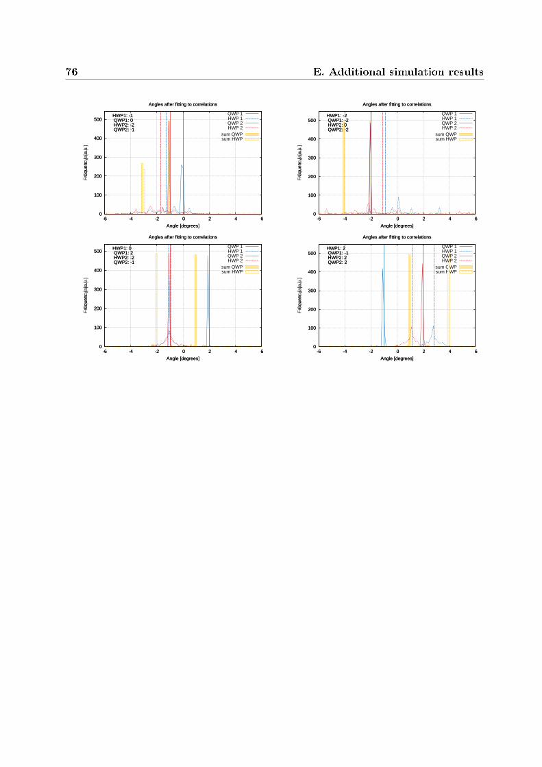
76 E. Additional simulation results

0

100

200

300

400

500

-6 -4 -2 0 2 4 6

Cou

nts

[a.u

.]

Angle [degrees]

Angles after fitting to correlations

HWP1: -1 QWP1: 0 HWP2: -2 QWP2: -1

sum QWPsum HWP

0

100

200

300

400

500

-6 -4 -2 0 2 4 6

Fre

quen

cy [

a.u.

]

Angle [degrees]

Angles after fitting to correlations

HWP1: -1 QWP1: 0 HWP2: -2 QWP2: -1

QWP 1HWP 1QWP 2HWP 2

0

100

200

300

400

500

-6 -4 -2 0 2 4 6

Cou

nts

[a.u

.]

Angle [degrees]

Angles after fitting to correlations

HWP1: -2 QWP1: -2 HWP2: 0 QWP2: -2

sum QWPsum HWP

0

100

200

300

400

500

-6 -4 -2 0 2 4 6

Fre

quen

cy [

a.u.

]

Angle [degrees]

Angles after fitting to correlations

HWP1: -2 QWP1: -2 HWP2: 0 QWP2: -2

QWP 1HWP 1QWP 2HWP 2

0

100

200

300

400

500

-6 -4 -2 0 2 4 6

Cou

nts

[a.u

.]

Angle [degrees]

Angles after fitting to correlations

HWP1: 0 QWP1: 2 HWP2: -2 QWP2: -1

sum QWPsum HWP

0

100

200

300

400

500

-6 -4 -2 0 2 4 6

Fre

quen

cy [

a.u.

]

Angle [degrees]

Angles after fitting to correlations

HWP1: 0 QWP1: 2 HWP2: -2 QWP2: -1

QWP 1HWP 1QWP 2HWP 2

0

100

200

300

400

500

-6 -4 -2 0 2 4 6

Cou

nts

[a.u

.]

Angle [degrees]

Angles after fitting to correlations

HWP1: 2 QWP1: -1 HWP2: 2 QWP2: 2

sum QWPsum HWP

0

100

200

300

400

500

-6 -4 -2 0 2 4 6

Fre

quen

cy [

a.u.

]

Angle [degrees]

Angles after fitting to correlations

HWP1: 2 QWP1: -1 HWP2: 2 QWP2: 2

QWP 1HWP 1QWP 2HWP 2

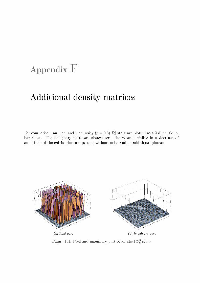
Appendix F

Additional density matrices

For comparison, an ideal and ideal noisy (p = 0.3) D36 state are plotted as a 3 dimensional

bar chart. The imaginary parts are always zero, the noise is visible in a decrease ofamplitude of the entries that are present without noise and an additional plateau.

(a) Real part (b) Imaginary part

Figure F.1: Real and imaginary part of an ideal D36 state

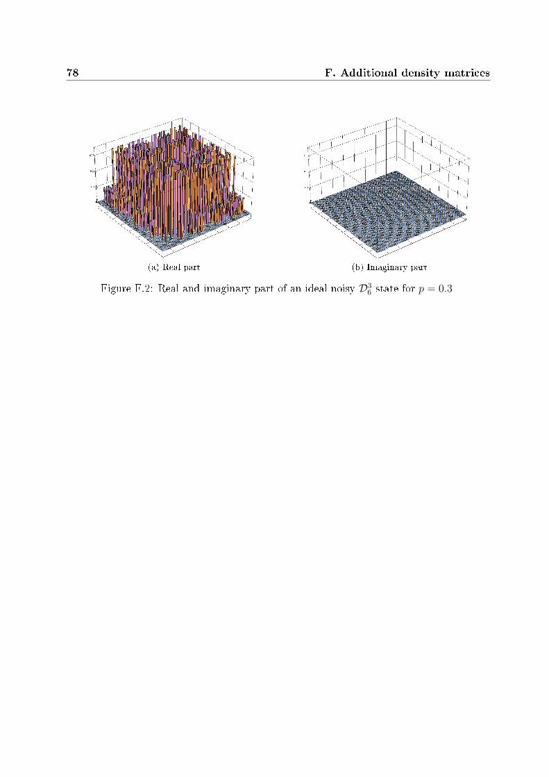
78 F. Additional density matrices

(a) Real part (b) Imaginary part

Figure F.2: Real and imaginary part of an ideal noisy D36 state for p = 0.3

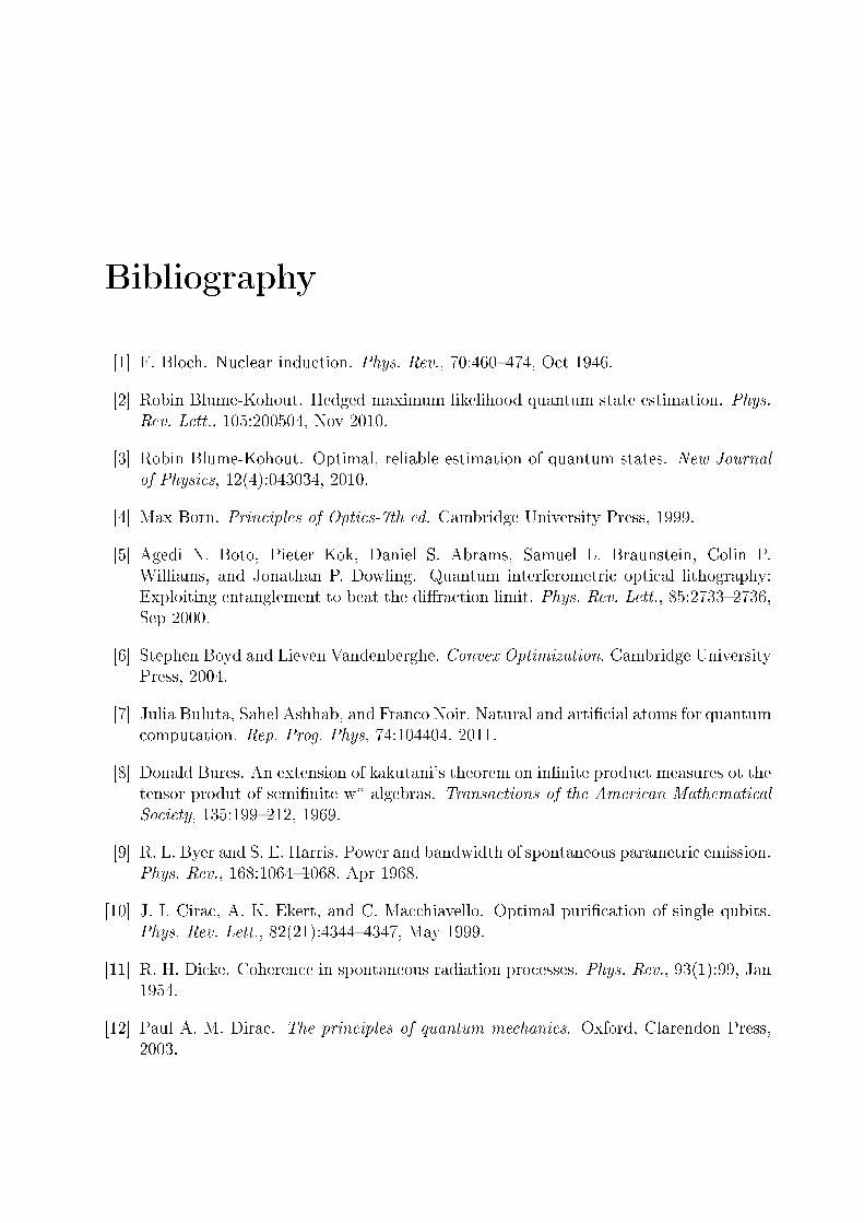
Bibliography

[1] F. Bloch. Nuclear induction. Phys. Rev., 70:460�474, Oct 1946.

[2] Robin Blume-Kohout. Hedged maximum likelihood quantum state estimation. Phys.Rev. Lett., 105:200504, Nov 2010.

[3] Robin Blume-Kohout. Optimal, reliable estimation of quantum states. New Journalof Physics, 12(4):043034, 2010.

[4] Max Born. Principles of Optics-7th ed. Cambridge University Press, 1999.

[5] Agedi N. Boto, Pieter Kok, Daniel S. Abrams, Samuel L. Braunstein, Colin P.Williams, and Jonathan P. Dowling. Quantum interferometric optical lithography:Exploiting entanglement to beat the di�raction limit. Phys. Rev. Lett., 85:2733�2736,Sep 2000.

[6] Stephen Boyd and Lieven Vandenberghe. Convex Optimization. Cambridge UniversityPress, 2004.

[7] Julia Buluta, Sahel Ashhab, and Franco Noir. Natural and arti�cial atoms for quantumcomputation. Rep. Prog. Phys, 74:104404, 2011.

[8] Donald Bures. An extension of kakutani's theorem on in�nite product measures ot thetensor produt of semi�nite w* algebras. Transactions of the American MathematicalSociety, 135:199�212, 1969.

[9] R. L. Byer and S. E. Harris. Power and bandwidth of spontaneous parametric emission.Phys. Rev., 168:1064�1068, Apr 1968.

[10] J. I. Cirac, A. K. Ekert, and C. Macchiavello. Optimal puri�cation of single qubits.Phys. Rev. Lett., 82(21):4344�4347, May 1999.

[11] R. H. Dicke. Coherence in spontaneous radiation processes. Phys. Rev., 93(1):99, Jan1954.

[12] Paul A. M. Dirac. The principles of quantum mechanics. Oxford, Clarendon Press,2003.

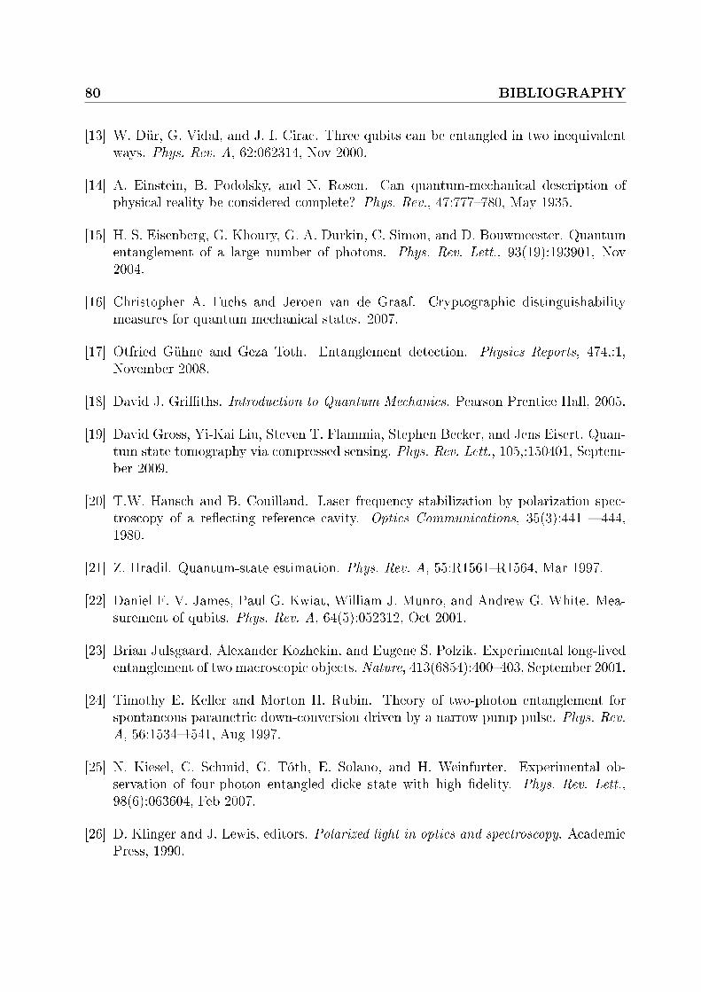
80 BIBLIOGRAPHY

[13] W. Dür, G. Vidal, and J. I. Cirac. Three qubits can be entangled in two inequivalentways. Phys. Rev. A, 62:062314, Nov 2000.

[14] A. Einstein, B. Podolsky, and N. Rosen. Can quantum-mechanical description ofphysical reality be considered complete? Phys. Rev., 47:777�780, May 1935.

[15] H. S. Eisenberg, G. Khoury, G. A. Durkin, C. Simon, and D. Bouwmeester. Quantumentanglement of a large number of photons. Phys. Rev. Lett., 93(19):193901, Nov2004.

[16] Christopher A. Fuchs and Jeroen van de Graaf. Cryptographic distinguishabilitymeasures for quantum mechanical states. 2007.

[17] Otfried Gühne and Geza Toth. Entanglement detection. Physics Reports, 474,:1,November 2008.

[18] David J. Gri�ths. Introduction to Quantum Mechanics. Pearson Prentice Hall, 2005.

[19] David Gross, Yi-Kai Liu, Steven T. Flammia, Stephen Becker, and Jens Eisert. Quan-tum state tomography via compressed sensing. Phys. Rev. Lett., 105,:150401, Septem-ber 2009.

[20] T.W. Hansch and B. Couillaud. Laser frequency stabilization by polarization spec-troscopy of a re�ecting reference cavity. Optics Communications, 35(3):441 � 444,1980.

[21] Z. Hradil. Quantum-state estimation. Phys. Rev. A, 55:R1561�R1564, Mar 1997.

[22] Daniel F. V. James, Paul G. Kwiat, William J. Munro, and Andrew G. White. Mea-surement of qubits. Phys. Rev. A, 64(5):052312, Oct 2001.

[23] Brian Julsgaard, Alexander Kozhekin, and Eugene S. Polzik. Experimental long-livedentanglement of two macroscopic objects. Nature, 413(6854):400�403, September 2001.

[24] Timothy E. Keller and Morton H. Rubin. Theory of two-photon entanglement forspontaneous parametric down-conversion driven by a narrow pump pulse. Phys. Rev.A, 56:1534�1541, Aug 1997.

[25] N. Kiesel, C. Schmid, G. Tóth, E. Solano, and H. Weinfurter. Experimental ob-servation of four-photon entangled dicke state with high �delity. Phys. Rev. Lett.,98(6):063604, Feb 2007.

[26] D. Klinger and J. Lewis, editors. Polarized light in optics and spectroscopy. AcademicPress, 1990.

BIBLIOGRAPHY 81

[27] Roland Krischek, Christian Schwemmer, Witlef Wieczorek, HaraldWeinfurter, PhilippHyllus, Luca Pezzé, and Augusto Smerzi. Useful multiparticle entanglement and sub-shot-noise sensitivity in experimental phase estimation. Phys. Rev. Lett., 107:080504,Aug 2011.

[28] Roland Krischek, Witlef Wieczorek, Akira Ozawa, Nikolai Kiesel, Patrick Michel-berger, Thomas Udem, and Harald Weinfurter. Ultraviolet enhancement cavity forultrafast nonlinear optics and high-rate multiphoton entanglement experiments. NatPhoton, 4(3):170�173, March 2010.

[29] Douglas Magde and Herbert Mahr. Study in ammonium dihydrogen phosphate ofspontaneous parametric interaction tunable from 4400 to 16 000 å. Phys. Rev. Lett.,18:905�907, May 1967.

[30] Harold Metcalf. Magneto-optical trapping and its application to helium metastables.J. Opt. Soc. Am. B, 6(11):2206�2210, Nov 1989.

[31] M.G.A Paris and J Rehacek, editors. Quantum State Estimation. Springer, 2004.

[32] G. J. Pryde, J. L. O'Brien, A. G. White, S. D. Bartlett, and T. C. Ralph. Measuringa photonic qubit without destroying it. Phys. Rev. Lett., 92:190402, May 2004.

[33] Michael Reimpell. Quantum Information and Convex Optimization. PhD thesis,Technische Universität Carolo-Wilhelmina, 2008.

[34] Jun J. Sakurai. Modern Quantum Mechanics. Addison-Wesley, 2005.

[35] B.A.E. Saleh and M.C. Teich. Fundamentals of Photonics. J. Wiley & Sons, 1991.

[36] Marek Sasura and Vladimír Buzek. Cold trapped ions as quantum information pro-cessors. Journal of Modern Optics, 49(10):1593 � 1647, 2002.

[37] Benjamin Schumacher. Quantum coding. Phys. Rev. A, 51:2738�2747, Apr 1995.

[38] Franz Schwabel. Quantum Mechanics. Springer, 2007.

[39] John K. Stockton, J. M. Geremia, Andrew C. Doherty, and Hideo Mabuchi. Charac-terizing the entanglement of symmetric many-particle spin-1

2systems. Phys. Rev. A,

67(2):022112, Feb 2003.

[40] G. Toth, W. Wieczorek, D. Gross, R. Krischek, C. Schwemmer, and H. Weinfurter.Permutationally invariant quantum tomography. Phys. Rev. Lett., 105(25):250403,Dec 2010.

[41] G. Toth, W. Wieczorek, D. Gross, R. Krischek, C. Schwemmer, and H. Weinfurter.Permutationally invariant quantum tomography (supplement). Phys. Rev. Lett.,105(25):250403, Dec 2010.

82 BIBLIOGRAPHY

[42] Geza Toth. Detection of multipartite entanglement in the vicinity of symmetric dickestates. J. Opt. Soc. Am. B, 24,:275, 2007.

[43] Pavel Trojek. E�cient Generation of Photonic Entanglement and Multiparty QuatumCommunication. PhD thesis, Ludwig Maximilians Universität München, 2007.

[44] J. von Neumann. Mathematische begründung der quantenmechanik. Nachrichtenvon der Gesellschaft der Wissenschaften zu Göttingen, Mathematisch-PhysikalischeKlasse, 1927.

[45] Reinhard F. Werner. Quantum states with einstein-podolsky-rosen correlations ad-mitting a hidden-variable model. Phys. Rev. A, 40:4277�4281, Oct 1989.

[46] Witlef Wieczorek. Multi-Photon Entanglement: Experimental Observation, Charac-terization, and Application of up to Six-Photon Entangled States. PhD thesis, LudwigMaximilians Universität München, 2009.

[47] Xing-Can Yao, Tian-Xiong Wang, Ping Xu, He Lu, Ge-Sheng Pan, Xiao-Hui Bao,Cheng-Zhi Peng, Chao-Yang Lu, Yu-Ao Chen, and Jian-Wei Pan. Observation ofeight-photon entanglement. May 2011.

Erklärung:

Hiermit erkläre ich, die vorliegende Arbeit selbständig verfasst zu haben und keineanderen als die in der Arbeit angegebnene Quellen und Hilfsmittel benutzt zu haben.

München den 27.10.2011