Embed Size (px)
Citation preview
Reentry Flows in Chemical Non-Equilibrium in Three-Dimensions
EDISSON SÁVIO DE GÓES MACIEL(1) and AMILCAR PORTO PIMENTA(2)
IEA- Aeronautical Engineering Division ITA – Aeronautical Technological Institute
Praça Mal. Eduardo Gomes, 50 – Vila das Acácias – São José dos Campos – SP – 12228-900 BRAZIL
(1)[email protected] and (2)[email protected] Abstract: - This work presents a numerical tool implemented to simulate inviscid and viscous flows employing the reactive gas formulation of thermal equilibrium and chemical non-equilibrium in three-dimensions. The Euler and Navier-Stokes equations, employing a finite volume formulation, on the context of structured and unstructured spatial discretizations, are solved. These variants allow an effective comparison between the two types of spatial discretization aiming verify their potentialities: solution quality, convergence speed, computational cost, etc. The aerospace problem involving the hypersonic flow around a blunt body, in three-dimensions, is simulated. The reactive simulations will involve an air chemical model of five species: N, N2, NO, O and O2. Seventeen chemical reactions, involving dissociation and recombination, will be simulated by the proposed model. The Arrhenius formula will be employed to determine the reaction rates and the law of mass action will be used to determine the source terms of each gas species equation. Key-Words: Euler and Navier-Stokes equations, Reactive formulation, Chemical non-equilibrium, Hypersonic flow, Van Leer algorithm, Three-dimensions. 1 Introduction
In several aerodynamic applications, the atmospheric air, even being composed of several chemical species, can be considered as a perfect thermal and caloric gas due to its inert property as well its uniform composition in space and constancy in time. However, there are several practical situations involving chemical reactions, as for example: combustion processes, flows around spatial vehicles in reentry conditions or plasma flows, which do not permit the ideal gas hypothesis ([1]). As described in [2], since these chemical reactions are very fast such that all processes can be considered in equilibrium, the conservation laws which govern the fluid become essentially unaltered, except that one equation to the general state of equilibrium has to be used opposed to the ideal gas law. When the flow is not in chemical equilibrium, one mass conservation law has to be written to each chemical species and the size of the equation system increases drastically.
Hypersonic flows are primary characterized by a very high level of energy ([3]). Through the shock wave, the kinetic energy is transformed in enthalpy. The flow temperature between the shock wave and the body is very high. Under such conditions, the air
properties are considerably modified. Phenomena like vibrational excitation and molecular dissociation of O2 and N2 frequently occur. The energy is stored under a form of free energy and the flow temperature is extremely reduced as compared with the temperature of an ideal gas flow. The thermodynamic and transport coefficients are not more constants. In summary, the ideal gas hypothesis is not truer and such flow is called the hypersonic flow of reactive gas or “hot gas flow”.
During the reentry and the hypersonic flights of aerospace vehicles in the atmosphere, reactive gas effects are present. The analysis of such hypersonic flows is critical to an appropriated aerodynamic and thermal project of such vehicles. The numerical simulation of reactive-gas-hypersonic flows is a very complex and disputed task. The present work emphasizes the numerical simulation of hypersonic flow in thermal equilibrium and chemical non-equilibrium. Some examples of works involving reactive gas flow are described below:
[1] developed upwind schemes based on residual distribution to the numerical simulation of inviscid flows of arbitrary mixtures of gases thermally perfect and in chemical non-equilibrium. They derived a multidimensional conservative
WSEAS TRANSACTIONS on MATHEMATICS Edisson Sávio De Góes Maciel, Amilcar Porto Pimenta
E-ISSN: 2224-2880 262 Issue 3, Volume 11, March 2012
linearization of the Euler equations to gas mixtures. After that, a transformation to a group of symmetrization variables was defined, which uncoupled the flow equations in “ns” scalar convection equations and a coupled 3x3 system. Several alternatives of discretization of the source terms were presented. Tests were accomplished with reactive and non-reactive flows.
[3] developed a computational code to the solution of the Reynolds averaged Navier-Stokes equations, employing an improved flux differencing splitting scheme of [4], which was more robust and did not require the implementation of an entropy condition. The code was developed to a structured finite difference context of spatial discretization. It was simulated the reactive-gas-hypersonic flow around a cylinder. Five chemical species were considered in the air chemical model: N, N2, NO, O and O2. It was considered seventeen chemical reactions, involving molecular dissociation and shuffle or exchange reactions. The law of mass action was employed aiming to determine the source terms to each chemical species in the expanded Navier-Stokes equations.
This work presents a numerical tool implemented to simulate inviscid and viscous flows employing the reactive gas formulation of thermal equilibrium and chemical non-equilibrium flow in three-dimensions. The Euler and Navier-Stokes equations, employing a finite volume formulation, on the context of structured and unstructured spatial discretizations, are solved. These variants allow an effective comparison between the two types of spatial discretization aiming verify their potentialities: solution quality, convergence speed, computational cost, etc. The aerospace problem of the “hot gas” hypersonic flow around a cylindrical blunt body is studied, in three-dimensions.
To the simulations with unstructured spatial discretization, a structured mesh generator developed by the first author ([5]), which create meshes of hexahedrons (3D), will be employed. After that, as a pre-processing stage ([6]), such meshes will be transformed in meshes of tetrahedrons. Such procedure aims to avoid the time which would be waste with the implementation of an unstructured generator, which is not the objective of the present work, and to obtain a generalized algorithm to the solution of the reactive equations.
The reactive simulations will involve an air chemical model of five species: N, N2, NO, O and
O2. Seventeen chemical reactions, involving dissociation and recombination ones, will be simulated by the proposed model. The Arrhenius formula will be employed to determine the reaction rates and the law of mass action will be used to determine the source terms of each gas species equation.
The algorithm employed to solve the reactive equations is the [7], first- and second-order accurate. The second-order numerical scheme is obtained by a “MUSCL” extrapolation process in the structured case (details in [8]). In the unstructured case, tests with the reconstruction linear process (details in [9]) did not yield converged results and, therefore, will not be presented. The algorithm will be implemented in a FORTRAN77 programming language, using the software Microsoft Developer Studio. Simulations in three microcomputers (one desktop and two notebooks) will be accomplished: one with processor Intel Celeron of 1.5 GHz of clock and 1.0 GBytes of RAM (notebook), one with processor AMD-Sempron of 1.87 GHz of clock and 512 MBytes of RAM (desktop) and the third one with processor Intel Celeron of 2.13 GHz of clock and 1.0 GBytes of RAM (notebook). The results have demonstrated that the most critical pressure field was obtained by the [7] scheme, first-order accurate, viscous and in its structured version. Moreover, in this case, the peak temperature reaches its maximum in this case. The cheapest algorithm was the [7] scheme, inviscid, first-order accurate and in its unstructured version. It is 115.51 % cheaper than the most expensive. The shock position determined by the thermal equilibrium and chemical non-equilibrium case is closer to the configuration nose than in the ideal gas case, ratifying the expected behavior highlighted in the CFD literature. 2 Formulation to Reactive Flow in Thermal Equilibrium and Chemical Non-Equilibrium
The Navier-Stokes reactive equations in thermal equilibrium and chemical non-equilibrium in the three-dimensional case, on a context of finite volumes, in integral and conservative forms can be expressed by:
∫ ∫∫ =•+∂∂
V VC
S
dVSdSnFQdVt
, (1)
with:
WSEAS TRANSACTIONS on MATHEMATICS Edisson Sávio De Góes Maciel, Amilcar Porto Pimenta
E-ISSN: 2224-2880 263 Issue 3, Volume 11, March 2012
( ) ( ) ( )kGGjFFiEEF veveve
−+−+−= , (2)
where Q is the vector of conserved variables, V is the computational cell volume, F
is the complete flux vector, n is the unit vector normal to the flux face, S is the flux area, SC is the chemical source term, Ee, Fe and Ge are the convective flux vectors or Euler flux vectors in the x, y and z direction, respectively, and Ev, Fv and Gv are the viscous flux vectors in the x, y and z directions, respectively. The i
, j
and k
unit vectors define the Cartesian coordinate system. Nine (9) conservation equations are solved: one of general mass conservation, three of linear momentum conservation, one of total energy and four of species mass conservation. Therefore, one of the species is absent of the solution algorithm. The CFD (“Computational Fluid Dynamics”) literature recommends that the species to be omitted of the formulation should be that of biggest mass fraction of the gaseous mixture, aiming to result in the minimum numerical error accumulated, corresponding to the biggest constituent of the mixture (in the case, air). To the present study, in which is chosen an air chemical model composed of five (5) species (N, N2, NO, O and O2) and seventeen (17) chemical reactions, being fifteen (15) dissociation reactions (endothermic reactions), this species can be the N2 or the O2. The O2 was chosen as the absent species to the simulation. The Q, Ee, Fe, Ge, Ev, Fv, Gv and SC vectors can, so, be defined conform below ([3]).
,
4
3
2
1
=
ρρρρewρvρuρρ
Q ,
4
3
2
1
2
+
=
uρuρuρuρ
Huρuwρuvρ
puρuρ
Ee )2(;
4
3
2
1
2
+
=
vρvρvρvρ
Hvρvwρ
pvρuvρvρ
Fe
,
4
3
2
1
2
+=
wρwρwρwρ
Hwρpwρ
vwρuwρwρ
Ge )3(,
0
Re1
44
33
22
11
a
vρvρvρvρ
φqwτvτuττττ
E
x
x
x
x
xxxzxyxx
xz
xy
xx
v
−−−−
−−++=
,
0
Re1
44
33
22
11
−−−−
−−++=
y
y
y
y
yyyzyyxy
yz
yy
xy
v
vρvρvρvρ
φqwτvτuττττ
F )3(;
0
Re1
44
33
22
11
b
vρvρvρvρ
φqwτvτuττττ
G
z
z
z
z
zzzzyzxz
zz
yz
xz
v
−−−−
−−++=
and { }TC ωωωωS 432100000 = , (4)
where: ρ is the mixture density; u, v and w are the Cartesian velocity components in the x, y and z directions, respectively; p is the fluid static pressure; e is the fluid total energy; ρ1, ρ2, ρ3 and ρ4 are the densities of the N, N2, NO and O, respectively; H is the mixture total enthalpy; the τ’s are the components of the viscous stress tensor; qx, qy and qz are the components of the Fourier heat flux vector in the x, y and z directions, respectively; Re is the flow laminar Reynolds number; ρsvsx, ρsvsy and ρsvsz represent the species diffusion flux, defined according to the Fick law; φx, φy and φz are the mixture diffusion terms; and sω is the chemical source term of each species equation, defined by the law of mass action.
The viscous stresses, in N/m2, are determined, according to a Newtonian fluid model, by:
∂∂
+∂∂
+∂∂
−∂∂
=zw
yv
xuμ
xuμτ xx 3
22 ,
∂∂
+∂∂
=xv
yuμτ xy ,
∂∂
+∂∂
=xw
zuμτ xz ,
∂∂
+∂∂
+∂∂
−∂∂
=zw
yv
xuμ
yvμτ yy 3
22 ; (5)
∂∂
+∂∂
=yw
zvμτ yz ,
∂∂
+∂∂
+∂∂
−∂∂
=zw
yv
xuμ
zwμτ zz 3
22 , (6)
in which µ is the fluid molecular viscosity.
The components of the Fourier heat flux vector, which considers only thermal conduction, are determined by:
WSEAS TRANSACTIONS on MATHEMATICS Edisson Sávio De Góes Maciel, Amilcar Porto Pimenta
E-ISSN: 2224-2880 264 Issue 3, Volume 11, March 2012
xTkqx ∂∂
−= , yTkqy ∂∂
−= and zTkqz ∂∂
−= . (7)
The laminar Reynolds number is defined by:
∞
∞∞=μ
LVρRe , (8)
where “∞” represents freestream properties, V∞ represents the flow characteristic velocity and L is a characteristic length of the studied configuration.
The species diffusion terms, defined according to the Fick law, to a thermal equilibrium condition, are determined by ([3]):
xY
Dρvρ ssxs ∂
∂−= ,
yY
Dρvρ ssys ∂
∂−= and
z
YDρvρ s
szs ∂∂
−= , (9)
with “s” referent to a given species, Ys being the species mass fraction and D the binary diffusion coefficient of the mixture. The chemical species mass fraction “s” is defined by:
ρρY ss = (10)
and the binary diffusion coefficient of the mixture is defined by:
Cpρ
kLeD = , (11)
where: k is the mixture thermal conductivity; Le is the Lewis number, kept constant to thermal equilibrium, with value 1.4; and Cp is the mixture specific heat at constant pressure; and vsx, vsy and vsz are the diffusion velocities of the “s” species in the x, y and z directions, respectively. The mixture k is determined by the transport model and the mixture Cp is determined in the thermodynamic model.
The φx, φy and φz diffusion terms which appear in the energy equation are defined by ([3]):
∑=
=ns
sssxsx hvρφ
1
, ∑=
=ns
sssysy hvρφ
1
and
∑=
=ns
ssszsz hvρφ
1
, (12)
being hs the specific enthalpy (sensible) of the “s” chemical species. The thermodynamic model, the transport model and the chemical model are presented in [10]. However, in the thermodynamic model some complement definitions are necessary to the three-dimensional space. The mixture total energy is determined by:
( )
++++= ∑∑
==
222
1
0
1
21 wvuhYTCvYρens
sss
ns
sss , (13)
in the three-dimensional case, where:
ρ is the mixture density;
ns is the total number of chemical species;
Cvs is the specific heat at constant volume to each “s” chemical species, in J/(kg.K);
ss RCv 23= , to monatomic gas, in J/(kg.K); (14)
ss RCv 25= , to diatomic gas, in J/(kg.K); (15)
sunivs MRR = , gas specific constant of the “s” chemical species, in J/(kg.K); (16)
sM is the molecular weight of the species “s”;
T is the translacional/rotacional temperature;
∑=
=ns
ssshYh
1
00 is the mixture formation enthalpy;
(17)
0sh is the formation enthalpy of each “s”
chemical species (with value 0.0 to diatomic gases of the same species). The mixture total enthalpy is determined by:
)(5.0 222 wvuhH +++= , in the three-dimensions. (18)
The mixture translational/rotational temperature is obtained from Eq. (13), in the three-dimensional case:
( )
++−−= ∑∑
==
ns
sss
ns
sss CvYwvuhYρeT
1
222
1
0 21 . (19)
WSEAS TRANSACTIONS on MATHEMATICS Edisson Sávio De Góes Maciel, Amilcar Porto Pimenta
E-ISSN: 2224-2880 265 Issue 3, Volume 11, March 2012
3 Structured Algorithm of [7] in Three-Dimensions
The numerical procedure to the solution of the convective flux consists of decouple the Euler equations in two parts ([11]). One convective part associated with the dynamic flux of the reactive Euler equations and another convective part associated with the chemical flux of the reactive Euler equations. The decoupling is described below.
The approximation of the integral equation (1) to a hexahedral finite volume yields a system of ordinary differential equations with respect to time defined by:
kjikjikji RdtdQV ,,,,,, −= , (20)
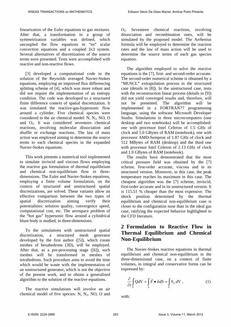
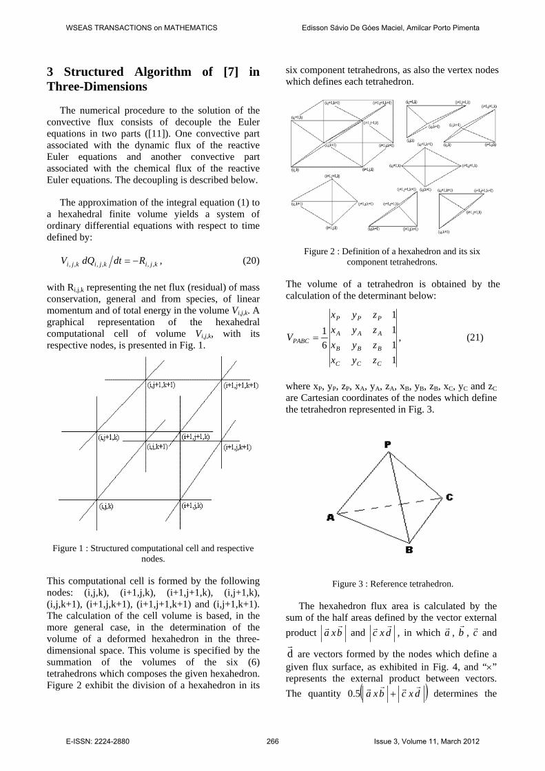
with Ri,j,k representing the net flux (residual) of mass conservation, general and from species, of linear momentum and of total energy in the volume Vi,j,k. A graphical representation of the hexahedral computational cell of volume Vi,j,k, with its respective nodes, is presented in Fig. 1.
Figure 1 : Structured computational cell and respective nodes.
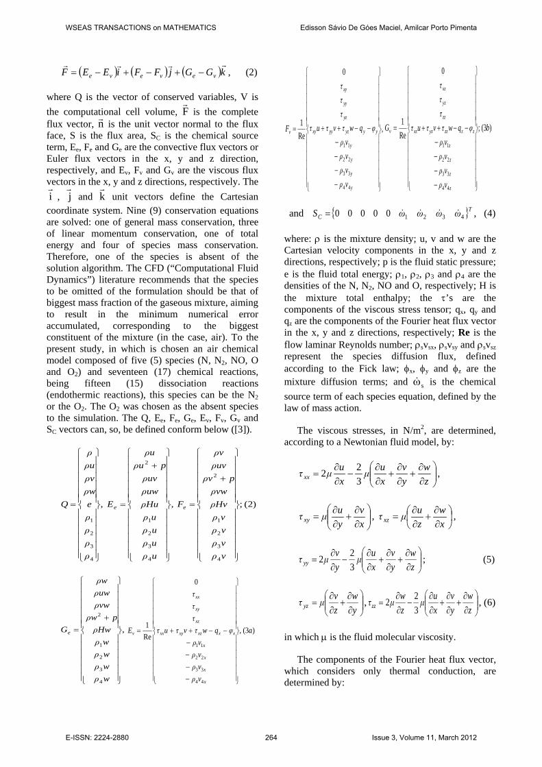
This computational cell is formed by the following nodes: (i,j,k), (i+1,j,k), (i+1,j+1,k), (i,j+1,k), (i,j,k+1), (i+1,j,k+1), (i+1,j+1,k+1) and (i,j+1,k+1). The calculation of the cell volume is based, in the more general case, in the determination of the volume of a deformed hexahedron in the three-dimensional space. This volume is specified by the summation of the volumes of the six (6) tetrahedrons which composes the given hexahedron. Figure 2 exhibit the division of a hexahedron in its
six component tetrahedrons, as also the vertex nodes which defines each tetrahedron.
Figure 2 : Definition of a hexahedron and its six component tetrahedrons.
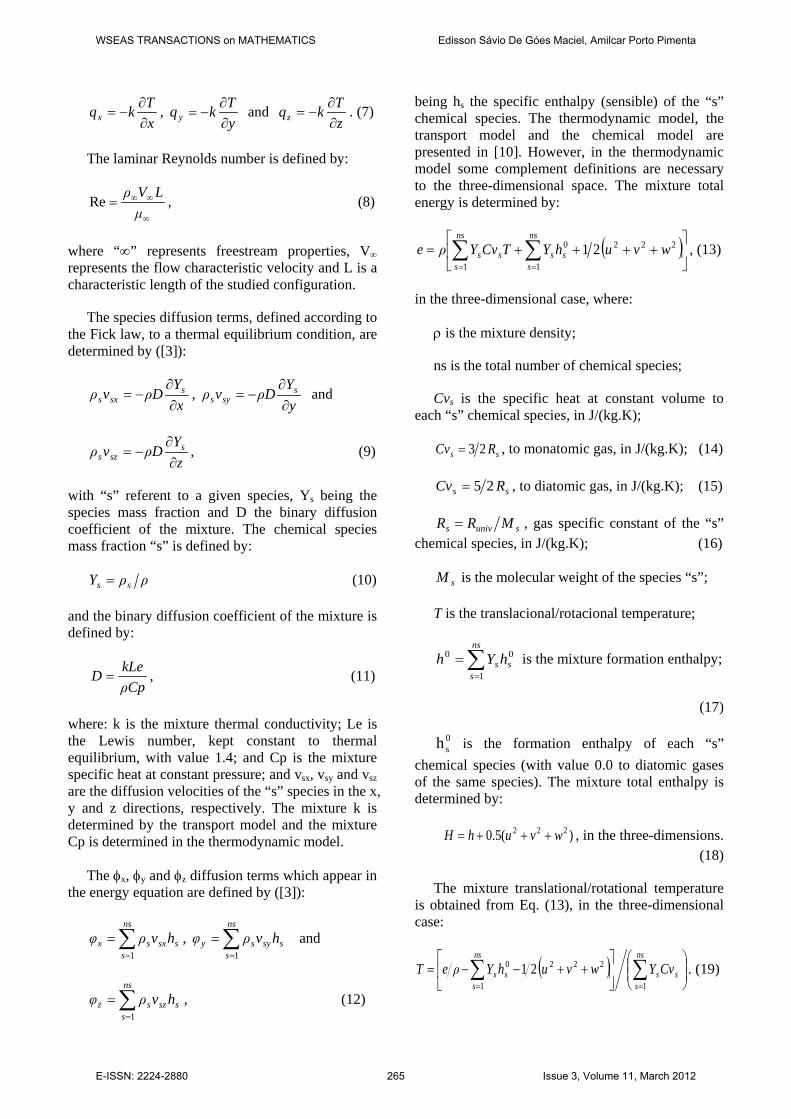
The volume of a tetrahedron is obtained by the calculation of the determinant below:
1111
61
CCC
BBB
AAA
PPP
PABC
zyxzyxzyxzyx
V = , (21)
where xP, yP, zP, xA, yA, zA, xB, yB, zB, xC, yC and zC are Cartesian coordinates of the nodes which define the tetrahedron represented in Fig. 3.
Figure 3 : Reference tetrahedron.
The hexahedron flux area is calculated by the sum of the half areas defined by the vector external product bxa
and dxc
, in which a , b
, c and
d
are vectors formed by the nodes which define a given flux surface, as exhibited in Fig. 4, and “×” represents the external product between vectors. The quantity ( )dxcbxa
+5.0 determines the
WSEAS TRANSACTIONS on MATHEMATICS Edisson Sávio De Góes Maciel, Amilcar Porto Pimenta
E-ISSN: 2224-2880 266 Issue 3, Volume 11, March 2012
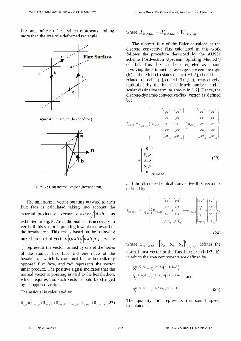
flux area of each face, which represents nothing more than the area of a deformed rectangle.
Figure 4 : Flux area (hexahedron).
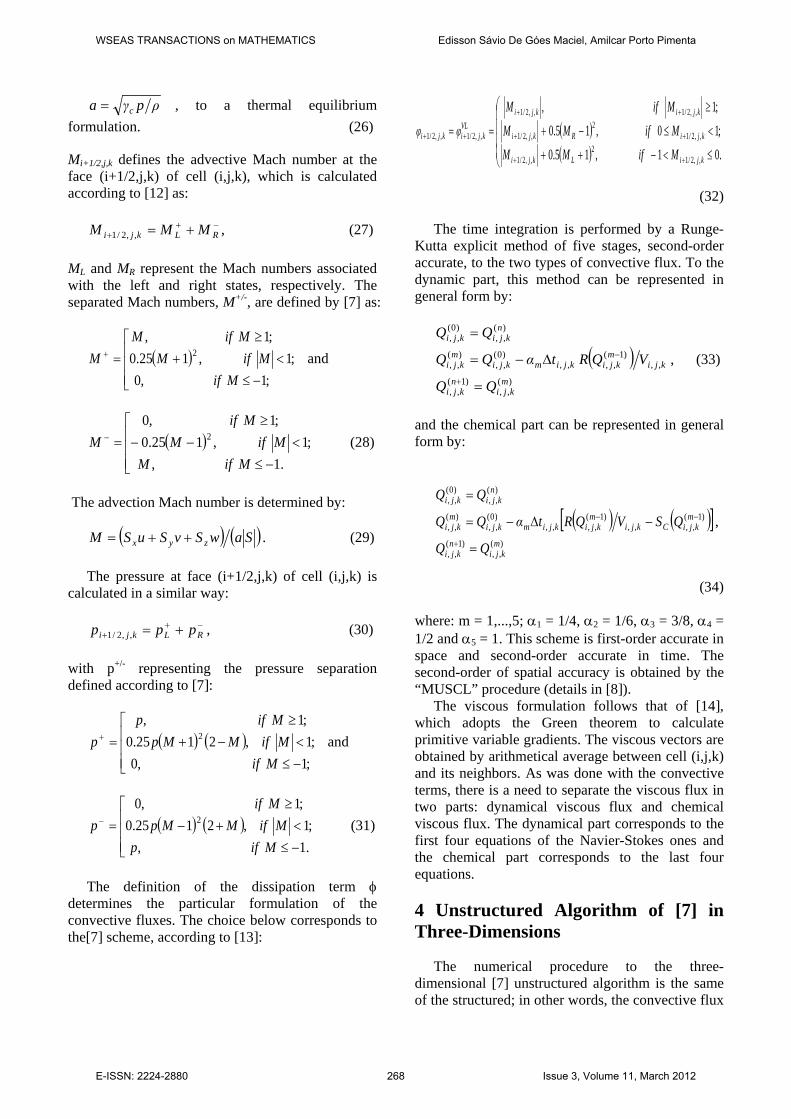
Figure 5 : Unit normal vector (hexahedron).
The unit normal vector pointing outward to each flux face is calculated taking into account the external product of vectors bxabxan
= , as
exhibited in Fig. 5. An additional test is necessary to verify if this vector is pointing inward or outward of the hexahedron. This test is based on the following mixed product of vectors [ ] fbxabxa
•)( , where
f
represents the vector formed by one of the nodes of the studied flux face and one node of the hexahedron which is contained in the immediately opposed flux face, and “•” represents the vector inner product. The positive signal indicates that the normal vector is pointing inward to the hexahedron, which requires that such vector should be changed by its opposed vector.
The residual is calculated as:
2/1k,j,i2/1k,j,ik,j,2/1ik,2/1j,ik,j,2/1ik,2/1j,ik,j,i RRRRRRR +−−++− +++++= , (22)
where vkj21i
ekj21ikj21i RRR ,,/,,/,,/ +++ −= .
The discrete flux of the Euler equations or the discrete convective flux calculated in this work follows the procedure described by the AUSM scheme (“Advection Upstream Splitting Method”) of [12]. This flux can be interpreted as a sum involving the arithmetical average between the right (R) and the left (L) states of the (i+1/2,j,k) cell face, related to cells (i,j,k) and (i+1,j,k), respectively, multiplied by the interface Mach number, and a scalar dissipative term, as shown in [12]. Hence, the discrete-dynamic-convective-flux vector is defined by:
−
−
+
= ++++
LR
kji
RL
kjikjikji
aHρawρavρauρaρ
aHρawρavρauρaρ
φ
aHρawρavρauρaρ
aHρawρavρauρaρ
MSR ,,2/1,,2/1,,2/1,,2/1 21
21
kji
z
y
x
pSpSpS
,,2/10
0
+
+ (23)
and the discrete-chemical-convective-flux vector is defined by:
,21
21
4
3
2
1
4
3
2
1
,,2/1
4
3
2
1
4
3
2
1
,,2/1,,2/1,,2/1
−
−
+
= ++++
LR
kji
RL
kjikjikji
aρaρaρaρ
aρaρaρaρ
φ
aρaρaρaρ
aρaρaρaρ
MSR ,
(24)
where [ ]Tkjizyxkji SSSS
,,2/1,,2/1 ++ = defines the
normal area vector to the flux interface (i+1/2,j,k), in which the area components are defined by:
( )kjikjix
kjix SnS ,,2/1,,2/1,,2/1 +++ = ,
( )kjikjiy
kjiy SnS ,,2/1,,2/1,,2/1 +++ = and
( )kjikjiz
kjiz SnS ,,2/1,,2/1,,2/1 +++ = . (25)
The quantity “a” represents the sound speed, calculated as:
WSEAS TRANSACTIONS on MATHEMATICS Edisson Sávio De Góes Maciel, Amilcar Porto Pimenta
E-ISSN: 2224-2880 267 Issue 3, Volume 11, March 2012
ρpγa c= , to a thermal equilibrium formulation. (26)
Mi+1/2,j,k defines the advective Mach number at the face (i+1/2,j,k) of cell (i,j,k), which is calculated according to [12] as:
−++ += RLkji MMM ,,2/1 , (27)
ML and MR represent the Mach numbers associated with the left and right states, respectively. The separated Mach numbers, M+/-, are defined by [7] as:
( ) ;1;1,0
,125.0;1,
2 <
−≤+
≥=+
MifMifM
MifMM and
( ) ;1.1,
,125.0;1,0
2 <
−≤−−
≥=−
MifMMifM
MifM (28)
The advection Mach number is determined by:
( ) ( )SawSvSuSM zyx ++= . (29)
The pressure at face (i+1/2,j,k) of cell (i,j,k) is calculated in a similar way:
−++ += RLkji ppp ,,2/1 , (30)
with p+/- representing the pressure separation defined according to [7]:
( ) ( )
−≤<−+
≥=+
;1,0;1,2125.0
;1,2
MifMifMMp
Mifpp and
( ) ( )
−≤<+−
≥=−
.1,;1,2125.0
;1,02
MifpMifMMp
Mifp (31)
The definition of the dissipation term φ determines the particular formulation of the convective fluxes. The choice below corresponds to the[7] scheme, according to [13]:
( )( )
≤<−++
<≤−+
≥
==
++
++
++
++
.01,15.0;10,15.0
;1,
,,2/12
,,2/1
,,2/12
,,2/1
,,2/1,,2/1
,,2/1,,2/1
kjiLkji
kjiRkji
kjikjiVL
kjikji
MifMMMifMM
MifMφφ
(32)
The time integration is performed by a Runge-Kutta explicit method of five stages, second-order accurate, to the two types of convective flux. To the dynamic part, this method can be represented in general form by:
( ))(,,
)1(,,
,,)1(
,,,,)0(,,
)(,,
)(,,
)0(,,
mkji
nkji
kjim
kjikjimkjim
kji
nkjikji
VQRtαQQ
=
∆−=
=
+
− , (33)
and the chemical part can be represented in general form by:
( ) ( )[ ])(,,
)1(,,
)1(,,,,
)1(,,,,
)0(,,
)(,,
)(,,
)0(,,
mkji
nkji
mkjiCkji
mkjikjimkji
mkji
nkjikji
QSVQRtαQQ
=
−∆−=
=
+
−− ,
(34)
where: m = 1,...,5; α1 = 1/4, α2 = 1/6, α3 = 3/8, α4 = 1/2 and α5 = 1. This scheme is first-order accurate in space and second-order accurate in time. The second-order of spatial accuracy is obtained by the “MUSCL” procedure (details in [8]). The viscous formulation follows that of [14], which adopts the Green theorem to calculate primitive variable gradients. The viscous vectors are obtained by arithmetical average between cell (i,j,k) and its neighbors. As was done with the convective terms, there is a need to separate the viscous flux in two parts: dynamical viscous flux and chemical viscous flux. The dynamical part corresponds to the first four equations of the Navier-Stokes ones and the chemical part corresponds to the last four equations. 4 Unstructured Algorithm of [7] in Three-Dimensions
The numerical procedure to the three-dimensional [7] unstructured algorithm is the same of the structured; in other words, the convective flux
WSEAS TRANSACTIONS on MATHEMATICS Edisson Sávio De Góes Maciel, Amilcar Porto Pimenta
E-ISSN: 2224-2880 268 Issue 3, Volume 11, March 2012
consists in decoupling the Euler equations in two parts ([11]). One convective part associated with the dynamic flux of the reactive Euler equations and the other convective part associated with the chemical flux of the reactive Euler equations. The decoupling follows the description below.
The approximation of the integral equation (1) to a tetrahedron finite volume yields a system of ordinary differential equations with respect to time defined by:
iii RdtdQV −= , (35)
with Ri representing the net flux (residual) of mass conservation, general and of the species, of linear momentum and of total energy at volume Vi.
A given computational cell in structured notation is composed by the following nodes: (i,j,k), (i+1,j,k), (i+1,j+1,k), (i,j+1,k), (i,j,k+1), (i+1,j,k+1), (i+1,j+1,k+1) and (i,j+1,k+1). Figure 1 exhibits a representation of the computational cell, which is a hexahedron in three-dimensions. A computational cell on an unstructured context is formed by the decomposition of the given hexahedron in its six tetrahedrons. Figure 2 exhibits the division of one hexahedron in its six tetrahedrons, as also the vertex nodes which define each tetrahedron and Fig. 6 shows the isolated computational cell.
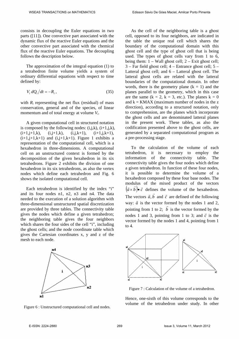
Each tetrahedron is identified by the index “i” and its four nodes n1, n2, n3 and n4. The data needed to the execution of a solution algorithm with three-dimensional unstructured spatial discretization are provided by three tables. The connectivity table gives the nodes which define a given tetrahedron; the neighboring table gives the four neighbors which shares the four sides of the cell “i”, including the ghost cells; and the node coordinate table which gives the Cartesian coordinates x, y and z of the mesh to each node.
Figure 6 : Unstructured computational cell and nodes.
As the cell of the neighboring table is a ghost cell, opposed to its four neighbors, are indicated in the table the unique real cell which shares the boundary of the computational domain with this ghost cell and the type of ghost cell that is being used. The types of ghost cells vary from 1 to 6, being them: 1 – Wall ghost cell; 2 – Exit ghost cell; 3 – Far field ghost cell; 4 – Entrance ghost cell; 5 – Latteral ghost cell; and 6 – Latteral ghost cell. The latteral ghost cells are related with the latteral boundaries of the computational domain. In other words, there is the geometry plane (k = 1) and the planes parallel to the geometry, which in this case are the same (k = 2, k = 3, etc.). The planes k = 0 and k = KMAX (maximum number of nodes in the z direction), according to a structured notation, only to comprehension, are the planes which incorporate the ghost cells and are denominated latteral planes in the present work. These tables, as also the codification presented above to the ghost cells, are generated by a separated computational program as a pre-processing stage.
To the calculation of the volume of each tetrahedron, it is necessary to employ the information of the connectivity table. The connectivity table gives the four nodes which define a given tetrahedron. In function of these four nodes, it is possible to determine the volume of a hexahedron composed by these four base nodes. The modulus of the mixed product of the vectors ( ) cba
•× defines the volume of the hexahedron. The vectors ba
, and c are defined of the following way: a is the vector formed by the nodes 1 and 2, pointing from 1 to 2; b
is the vector formed by the nodes 1 and 3, pointing from 1 to 3; and c is the vector formed by the nodes 1 and 4, pointing from 1 to 4.
Figure 7 : Calculation of the volume of a tetrahedron.
Hence, one-sixth of this volume corresponds to the volume of the tetrahedron under study. In other
WSEAS TRANSACTIONS on MATHEMATICS Edisson Sávio De Góes Maciel, Amilcar Porto Pimenta
E-ISSN: 2224-2880 269 Issue 3, Volume 11, March 2012
words, the hypothesis is that this hexahedron is composed by six tetrahedrons equal to that formed by the nodes 1, 2, 3 and 4. The graphic representation of this procedure is exhibited in Fig. 7. The same result to the calculation of the tetrahedron volume is obtained by the calculation of the following determinant:
1zyx1zyx1zyx1zyx
61V
444
333
222
111
1234 = , (36)
where x1, y1, z1, x2, y2, z2, x3, y3, z3, x4, y4 and z4 are the Cartesian coordinates of the nodes which define the tetrahedron represented in Fig. 7.
The flux area of a given tetrahedron is calculated by half of the norm of the external product bxa
, as indicated in Fig. 8. In this figure, it is possible to percept that the vector a is formed by the nodes 1 and 2, pointing from 1 to 2, and the vector b
is formed by the nodes 2 and 3, pointing from 2 to 3.
Figure 8 : Flux area (tetrahedron).
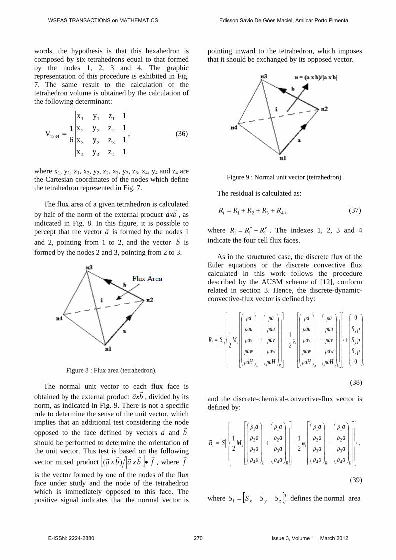
The normal unit vector to each flux face is obtained by the external product bxa
, divided by its norm, as indicated in Fig. 9. There is not a specific rule to determine the sense of the unit vector, which implies that an additional test considering the node opposed to the face defined by vectors a and b
should be performed to determine the orientation of the unit vector. This test is based on the following vector mixed product [ ] fbxabxa
•)( , where f
is the vector formed by one of the nodes of the flux face under study and the node of the tetrahedron which is immediately opposed to this face. The positive signal indicates that the normal vector is
pointing inward to the tetrahedron, which imposes that it should be exchanged by its opposed vector.
Figure 9 : Normal unit vector (tetrahedron).
The residual is calculated as:
4321 RRRRRi +++= , (37)
where ve RRR 111 −= . The indexes 1, 2, 3 and 4 indicate the four cell flux faces.
As in the structured case, the discrete flux of the Euler equations or the discrete convective flux calculated in this work follows the procedure described by the AUSM scheme of [12], conform related in section 3. Hence, the discrete-dynamic-convective-flux vector is defined by:
l
z
y
x
LR
l
RL
lll
pSpSpS
aHρawρavρauρaρ
aHρawρavρauρaρ
φ
aHρawρavρauρaρ
aHρawρavρauρaρ
MSR
+
−
−
+
=
0
0
21
21
(38)
and the discrete-chemical-convective-flux vector is defined by:
−
−
+
=
LR
l
RL
lll
aρaρaρaρ
aρaρaρaρ
φ
aρaρaρaρ
aρaρaρaρ
MSR
4
3
2
1
4
3
2
1
4
3
2
1
4
3
2
1
21
21 ,
(39)
where [ ]Tlzyxl SSSS = defines the normal area
WSEAS TRANSACTIONS on MATHEMATICS Edisson Sávio De Góes Maciel, Amilcar Porto Pimenta
E-ISSN: 2224-2880 270 Issue 3, Volume 11, March 2012
vector to the flux interface “l”. Ml defines the advective Mach number at the face “l” of cell “i”, which is calculated according to Eqs. (27) and (28). The advection Mach number is defined conform Eq. (29). The pressure at face “l” of cell “i” is calculated according to Eqs. (30) and (31).
The definition of the dissipation term φ determines the particular formulation of the convective fluxes. The choice below, as in the structured case, corresponds to the [7] scheme, according to [13]:
( )( )
≤<−++<≤−+≥
==.01,15,0;10,15,0
;1,
2
2
lLl
lRl
llVLll
MifMMMifMM
MifMφφ
(40)
The time integration is performed employing an explicit Runge-Kutta method of five stages, second-order accurate in time, to the two types of convective flow. To the dynamic part, this method can be represented in general form by:
( ))()1(
)1()0()(
)()0(
mi
ni
im
iimim
i
nii
VQRtαQQ
=
∆−=
=
+
− , (41)
and the chemical part can be represented in the general form by:
( ) ( )[ ])()1(
)1()1()0()(
)()0(
mi
ni
miCi
miimi
mi
nii
QSVQRtαQQ
=
−∆−=
=
+
−− , (42)
where m = 1,...,5; α1 = 1/4, α2 = 1/6, α3 = 3/8, α4 = 1/2 and α5 = 1. This scheme is first-order accurate in space and second-order in time. The viscous formulation follows that of [14], reported in section 3 of the present work. They adopt the Green theorem to calculate primitive variable gradients. The viscous vectors are obtained by arithmetical average between cell i and its neighbors. As was done with the convective terms, there is a need to separate the viscous flux in two parts: dynamical viscous flux and chemical viscous flux. The dynamical part corresponds to the first four equations of the Navier-Stokes ones and the chemical part corresponds to the last four equations.
5 Spatially Variable Time Step
A spatially variable time step was employed in this work. This technique has provided excellent convergence gains as demonstrated in [15-16] and is implemented in the codes presented in this work.
The basic idea of such procedure consists in keeping a constant CFL number in all computational domain, allowing, hence, that appropriated time steps to each specific mesh region can be used during the convergence process. Hence, according to the definition of the CFL number, it is possible to write:
( ) cellcellcell csCFLt ∆=∆ , (43)
where: CFL is the number of “Courant-Friedrichs-Lewy” to provide numerical stability to the scheme;
( )cell
cell awvuc
+++=
5.0222 is the maximum
characteristic velocity of propagation of information in the calculation domain; and ( )cells∆ is the characteristic length of propagation of information. On the context of finite volumes, ( )cells∆ is chosen as the minimum value found between the baricenter distance, involving the cell under study and its neighbors, and the minimum cell side length. 6 Results
Tests were performed in three microcomputers: one with INTEL CELERON processor, 1.5 GHz of clock and 1.0 GBytes of RAM (notebook), the second with an AMD SEMPRON (tm) 2600+ processor, 1.83 GHz of clock and 512 MBytes of RAM (desktop) and the third with an INTEL CELERON processor, 2.13 GHz of clock and 1.0 GBytes of RAM (notebook). As the interest of this work is steady state problems, it is necessary to define a criterion which guarantees the convergence of the numerical method. The criterion adopted was to consider a reduction of no minimal three (3) orders of magnitude in the value of the maximum residual in the calculation domain, a typical CFD community criterion. The residual of each cell was defined as the numerical value obtained from the discretized conservation equations. As there are nine (9) conservation equations to each cell, the maximum value obtained from these equations is defined as the residual of this cell. Hence, this residual is compared with the residual of the other cells, calculated of the same way, to define the
WSEAS TRANSACTIONS on MATHEMATICS Edisson Sávio De Góes Maciel, Amilcar Porto Pimenta
E-ISSN: 2224-2880 271 Issue 3, Volume 11, March 2012
maximum residual in the calculation domain. In the three-dimensional simulations, the angles at the perpendicular plane to the configuration, α, and at the longitudinal plane to the configuration, ψ, were considered equal to zero.
6.1 Initial and boundary conditions to the studied problem
The reactive flow in thermal equilibrium and chemical non-equilibrium to the cylindrical blunt body problem in three-dimensions was studied in this work. Table 1 presents the initial conditions to the problem of the cylindrical blunt body submitted to a reactive flow. The Reynolds number was calculated based on data from [17]. The boundary conditions to this problem of reactive flow are detailed in [18], as well the geometry in study, the meshes employed in the simulations and the description of the computational configuration. The geometry is a blunt body with 1.0 m of nose ratio and inclined rectilinear walls. The angle of inclination of the geometry walls is 10°. The far field is located at 20.0 times the nose ratio in relation to the configuration nose.
Table 1 : Initial conditions to problem of the blunt body.
Property Value
M∞ 8.78
ρ∞ 0.00326 kg/m3
p∞ 687 Pa
U∞ 4,776 m/s
T∞ 694 K
altitude 40,000 m
YN 10-9
2NY 0.73555
YNO 0.05090
YO 0.07955
l 3.76 m
Re∞ 4.4905x10⁶
The nondimensionalization employed in the Euler and Navier-Stokes equations in this study is also described in [18].
6.2 Studied cases
Table 2 presents the studied cases in this work, the mesh characteristics and the order of accuracy of the [7] scheme.
6.3 Results in thermal equilibrium and chemical non-equilibrium
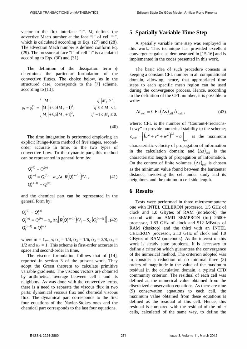
6.3.1 Inviscid, structured and first-order accurate case Figure 10 presents the pressure contours around the cylindrical blunt body in the three-dimensional computational domain. As can be observed, the contours curves are the same at planes k = constant, which represents the correct solution, because of the flow is effectively two-dimensional. However, the shock should be closer to the blunt body nose due to the dispersion effect inherent to the third dimension (z).
Table 2. Studied cases, mesh characteristics and accuracy order.
Case Mesh Accuracy order
Inviscid – 3D 63x60x10 Firsta
Viscous – 3D 63x60x10 (7.5%)c
Firsta
Inviscid – 3D 63x60x10 Seconda
Viscous – 3D 63x60x10 (7.5%)
Seconda
Inviscid – 3D 43x50x10 Firstb
Viscous – 3D 43x50x10 (3.0%)
Firstb
a Structured spatial discretization; b Unstructured spatial discretization; c Exponential stretching.
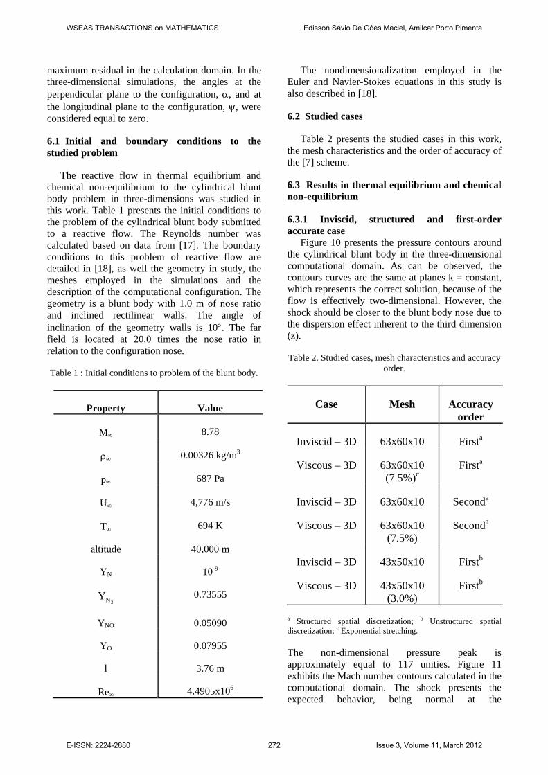
The non-dimensional pressure peak is approximately equal to 117 unities. Figure 11 exhibits the Mach number contours calculated in the computational domain. The shock presents the expected behavior, being normal at the
WSEAS TRANSACTIONS on MATHEMATICS Edisson Sávio De Góes Maciel, Amilcar Porto Pimenta
E-ISSN: 2224-2880 272 Issue 3, Volume 11, March 2012
configuration nose, oblique along the body wall and a Mach wave far from the blunt body geometry. The Mach number contours at plane k = 1 is repeated in the other planes k = constant.
Figure 10 : Pressure contours.
Figure 11 : Mach number contours.
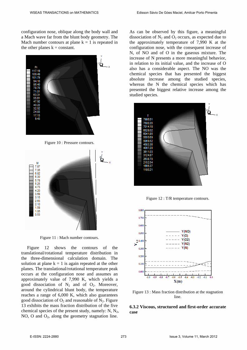
Figure 12 shows the contours of the translational/rotational temperature distribution in the three-dimensional calculation domain. The solution at plane k = 1 is again repeated at the other planes. The translational/rotational temperature peak occurs at the configuration nose and assumes an approximately value of 7,990 K, which yields a good dissociation of N2 and of O2. Moreover, around the cylindrical blunt body, the temperature reaches a range of 6,000 K, which also guarantees good dissociation of O2 and reasonable of N2. Figure 13 exhibits the mass fraction distribution of the five chemical species of the present study, namely: N, N2, NO, O and O2, along the geometry stagnation line.
As can be observed by this figure, a meaningful dissociation of N2 and O2 occurs, as expected due to the approximately temperature of 7,990 K at the configuration nose, with the consequent increase of N, of NO and of O in the gaseous mixture. The increase of N presents a more meaningful behavior, in relation to its initial value, and the increase of O also has a considerable aspect. The NO was the chemical species that has presented the biggest absolute increase among the studied species, whereas the N the chemical species which has presented the biggest relative increase among the studied species.
Figure 12 : T/R temperature contours.
Figure 13 : Mass fraction distribution at the stagnation line.
6.3.2 Viscous, structured and first-order accurate case
WSEAS TRANSACTIONS on MATHEMATICS Edisson Sávio De Góes Maciel, Amilcar Porto Pimenta
E-ISSN: 2224-2880 273 Issue 3, Volume 11, March 2012
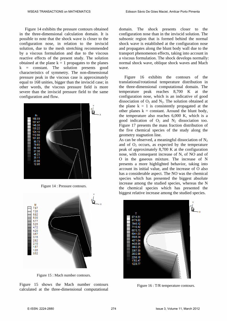
Figure 14 exhibits the pressure contours obtained in the three-dimensional calculation domain. It is possible to note that the shock wave is closer to the configuration nose, in relation to the inviscid solution, due to the mesh stretching recommended by a viscous formulation and due to the viscous reactive effects of the present study. The solution obtained at the plane k = 1 propagates to the planes k = constant. The solution presents good characteristics of symmetry. The non-dimensional pressure peak in the viscous case is approximately equal to 168 unities, bigger than the inviscid case; in other words, the viscous pressure field is more severe than the inviscid pressure field to the same configuration and flow.
Figure 14 : Pressure contours.
Figure 15 : Mach number contours.
Figure 15 shows the Mach number contours calculated at the three-dimensional computational
domain. The shock presents closer to the configuration nose than in the inviscid solution. The subsonic region that is formed behind the normal shock wave is established at the configuration nose and propagates along the blunt body wall due to the transport phenomenon effects, taking into account in a viscous formulation. The shock develops normally: normal shock wave, oblique shock waves and Mach wave.
Figure 16 exhibits the contours of the translational/rotational temperature distribution in the three-dimensional computational domain. The temperature peak reaches 8,700 K at the configuration nose, which is an indicative of good dissociation of O2 and N2. The solution obtained at the plane k = 1 is consistently propagated at the other planes k = constant. Around the blunt body, the temperature also reaches 6,000 K, which is a good indication of O2 and N2 dissociation too. Figure 17 presents the mass fraction distribution of the five chemical species of the study along the geometry stagnation line. As can be observed, a meaningful dissociation of N2 and of O2 occurs, as expected by the temperature peak of approximately 8,700 K at the configuration nose, with consequent increase of N, of NO and of O in the gaseous mixture. The increase of N presents a more highlighted behavior, taking into account its initial value, and the increase of O also has a considerable aspect. The NO was the chemical species which has presented the biggest absolute increase among the studied species, whereas the N the chemical species which has presented the biggest relative increase among the studied species.
Figure 16 : T/R temperature contours.
WSEAS TRANSACTIONS on MATHEMATICS Edisson Sávio De Góes Maciel, Amilcar Porto Pimenta
E-ISSN: 2224-2880 274 Issue 3, Volume 11, March 2012
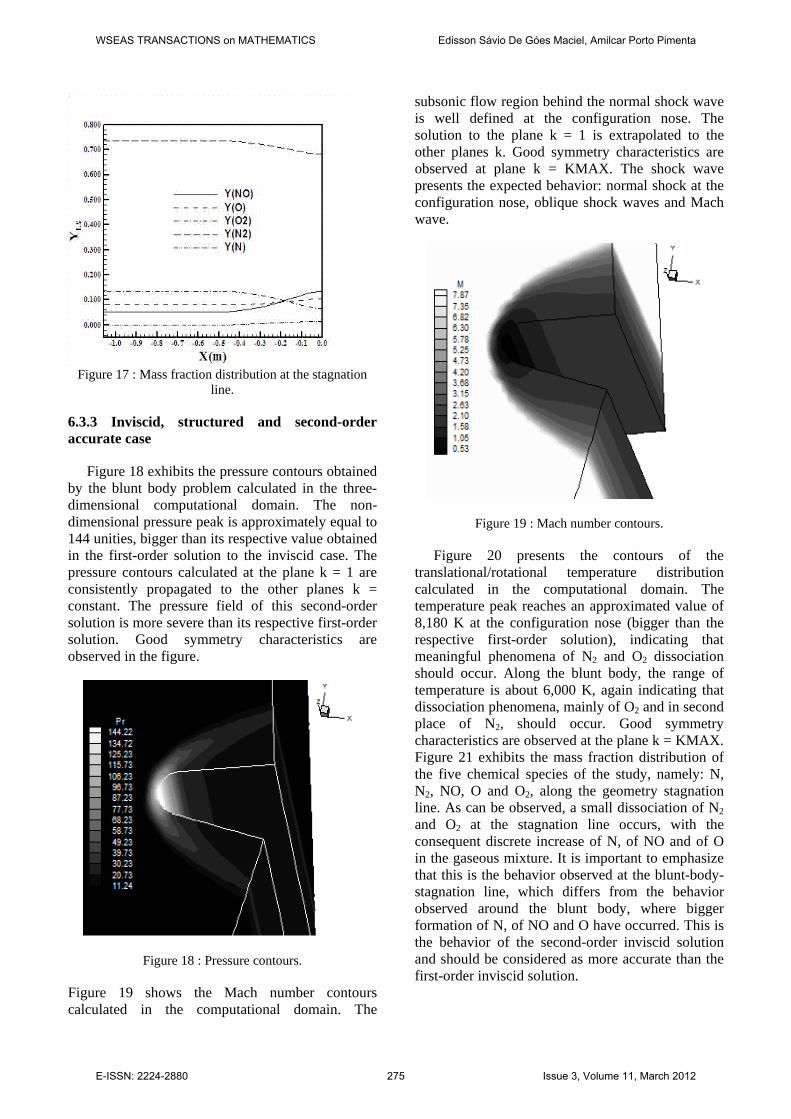
Figure 17 : Mass fraction distribution at the stagnation
line.
6.3.3 Inviscid, structured and second-order accurate case
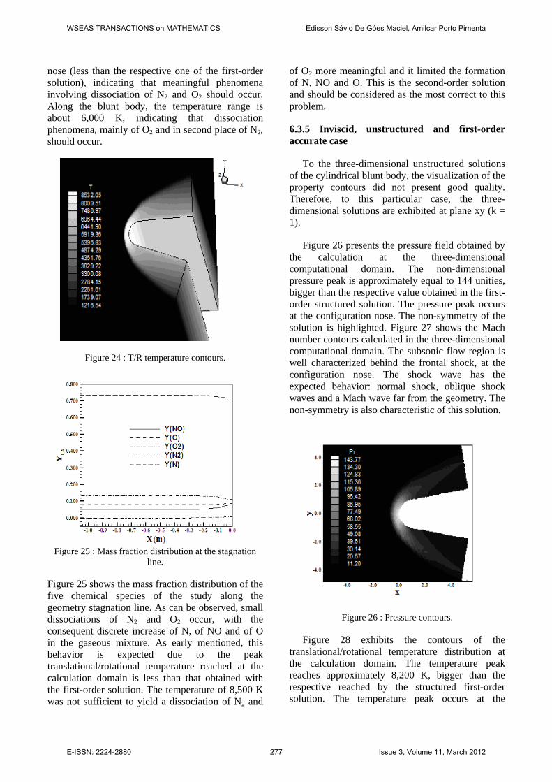
Figure 18 exhibits the pressure contours obtained by the blunt body problem calculated in the three-dimensional computational domain. The non-dimensional pressure peak is approximately equal to 144 unities, bigger than its respective value obtained in the first-order solution to the inviscid case. The pressure contours calculated at the plane k = 1 are consistently propagated to the other planes k = constant. The pressure field of this second-order solution is more severe than its respective first-order solution. Good symmetry characteristics are observed in the figure.
Figure 18 : Pressure contours.
Figure 19 shows the Mach number contours calculated in the computational domain. The
subsonic flow region behind the normal shock wave is well defined at the configuration nose. The solution to the plane k = 1 is extrapolated to the other planes k. Good symmetry characteristics are observed at plane k = KMAX. The shock wave presents the expected behavior: normal shock at the configuration nose, oblique shock waves and Mach wave.
Figure 19 : Mach number contours.
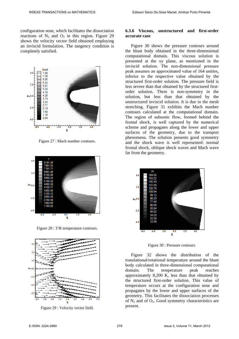
Figure 20 presents the contours of the translational/rotational temperature distribution calculated in the computational domain. The temperature peak reaches an approximated value of 8,180 K at the configuration nose (bigger than the respective first-order solution), indicating that meaningful phenomena of N2 and O2 dissociation should occur. Along the blunt body, the range of temperature is about 6,000 K, again indicating that dissociation phenomena, mainly of O2 and in second place of N2, should occur. Good symmetry characteristics are observed at the plane k = KMAX. Figure 21 exhibits the mass fraction distribution of the five chemical species of the study, namely: N, N2, NO, O and O2, along the geometry stagnation line. As can be observed, a small dissociation of N2 and O2 at the stagnation line occurs, with the consequent discrete increase of N, of NO and of O in the gaseous mixture. It is important to emphasize that this is the behavior observed at the blunt-body-stagnation line, which differs from the behavior observed around the blunt body, where bigger formation of N, of NO and O have occurred. This is the behavior of the second-order inviscid solution and should be considered as more accurate than the first-order inviscid solution.
WSEAS TRANSACTIONS on MATHEMATICS Edisson Sávio De Góes Maciel, Amilcar Porto Pimenta
E-ISSN: 2224-2880 275 Issue 3, Volume 11, March 2012
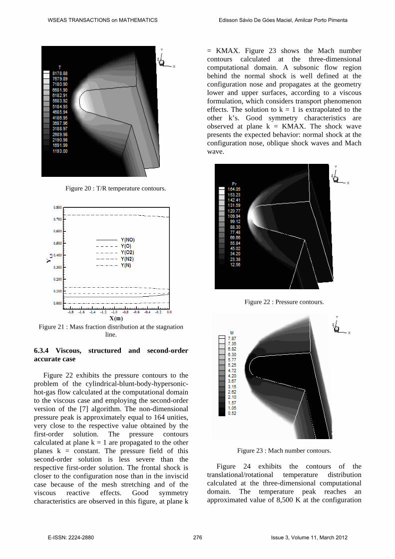
Figure 20 : T/R temperature contours.
Figure 21 : Mass fraction distribution at the stagnation
line.
6.3.4 Viscous, structured and second-order accurate case
Figure 22 exhibits the pressure contours to the problem of the cylindrical-blunt-body-hypersonic-hot-gas flow calculated at the computational domain to the viscous case and employing the second-order version of the [7] algorithm. The non-dimensional pressure peak is approximately equal to 164 unities, very close to the respective value obtained by the first-order solution. The pressure contours calculated at plane k = 1 are propagated to the other planes k = constant. The pressure field of this second-order solution is less severe than the respective first-order solution. The frontal shock is closer to the configuration nose than in the inviscid case because of the mesh stretching and of the viscous reactive effects. Good symmetry characteristics are observed in this figure, at plane k
= KMAX. Figure 23 shows the Mach number contours calculated at the three-dimensional computational domain. A subsonic flow region behind the normal shock is well defined at the configuration nose and propagates at the geometry lower and upper surfaces, according to a viscous formulation, which considers transport phenomenon effects. The solution to k = 1 is extrapolated to the other k’s. Good symmetry characteristics are observed at plane k = KMAX. The shock wave presents the expected behavior: normal shock at the configuration nose, oblique shock waves and Mach wave.
Figure 22 : Pressure contours.
Figure 23 : Mach number contours. Figure 24 exhibits the contours of the translational/rotational temperature distribution calculated at the three-dimensional computational domain. The temperature peak reaches an approximated value of 8,500 K at the configuration
WSEAS TRANSACTIONS on MATHEMATICS Edisson Sávio De Góes Maciel, Amilcar Porto Pimenta
E-ISSN: 2224-2880 276 Issue 3, Volume 11, March 2012
nose (less than the respective one of the first-order solution), indicating that meaningful phenomena involving dissociation of N2 and O2 should occur. Along the blunt body, the temperature range is about 6,000 K, indicating that dissociation phenomena, mainly of O2 and in second place of N2, should occur.
Figure 24 : T/R temperature contours.
Figure 25 : Mass fraction distribution at the stagnation
line. Figure 25 shows the mass fraction distribution of the five chemical species of the study along the geometry stagnation line. As can be observed, small dissociations of N2 and O2 occur, with the consequent discrete increase of N, of NO and of O in the gaseous mixture. As early mentioned, this behavior is expected due to the peak translational/rotational temperature reached at the calculation domain is less than that obtained with the first-order solution. The temperature of 8,500 K was not sufficient to yield a dissociation of N2 and
of O2 more meaningful and it limited the formation of N, NO and O. This is the second-order solution and should be considered as the most correct to this problem.
6.3.5 Inviscid, unstructured and first-order accurate case
To the three-dimensional unstructured solutions of the cylindrical blunt body, the visualization of the property contours did not present good quality. Therefore, to this particular case, the three-dimensional solutions are exhibited at plane xy (k = 1).
Figure 26 presents the pressure field obtained by the calculation at the three-dimensional computational domain. The non-dimensional pressure peak is approximately equal to 144 unities, bigger than the respective value obtained in the first-order structured solution. The pressure peak occurs at the configuration nose. The non-symmetry of the solution is highlighted. Figure 27 shows the Mach number contours calculated in the three-dimensional computational domain. The subsonic flow region is well characterized behind the frontal shock, at the configuration nose. The shock wave has the expected behavior: normal shock, oblique shock waves and a Mach wave far from the geometry. The non-symmetry is also characteristic of this solution.
Figure 26 : Pressure contours.
Figure 28 exhibits the contours of the translational/rotational temperature distribution at the calculation domain. The temperature peak reaches approximately 8,200 K, bigger than the respective reached by the structured first-order solution. The temperature peak occurs at the
WSEAS TRANSACTIONS on MATHEMATICS Edisson Sávio De Góes Maciel, Amilcar Porto Pimenta
E-ISSN: 2224-2880 277 Issue 3, Volume 11, March 2012
configuration nose, which facilitates the dissociation reactions of N2 and O2 in this region. Figure 29 shows the velocity vector field obtained employing an inviscid formulation. The tangency condition is completely satisfied.
Figure 27 : Mach number contours.
Figure 28 : T/R temperature contours.
Figure 29 : Velocity vector field.
6.3.6 Viscous, unstructured and first-order accurate case
Figure 30 shows the pressure contours around the blunt body obtained in the three-dimensional computational domain. This viscous solution is presented at the xy plane, as mentioned in the inviscid solution. The non-dimensional pressure peak assumes an approximated value of 164 unities, inferior to the respective value obtained by the structured first-order solution. The pressure field is less severe than that obtained by the structured first-order solution. There is non-symmetry in the solution, but less than that obtained by the unstructured inviscid solution. It is due to the mesh stretching. Figure 31 exhibits the Mach number contours calculated at the computational domain. The region of subsonic flow, formed behind the frontal shock, is well captured by the numerical scheme and propagates along the lower and upper surfaces of the geometry, due to the transport phenomena. The solution presents good symmetry and the shock wave is well represented: normal frontal shock, oblique shock waves and Mach wave far from the geometry.
Figure 30 : Pressure contours.
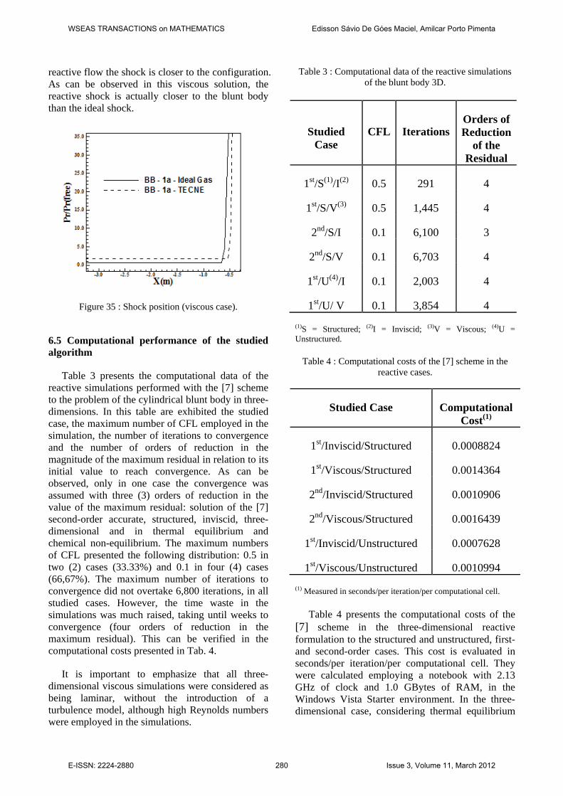
Figure 32 shows the distribution of the translational/rotational temperature around the blunt body calculated in three-dimensional computational domain. The temperature peak reaches approximately 8,200 K, less than that obtained by the structured first-order solution. This value of temperature occurs at the configuration nose and propagates by the lower and upper surfaces of the geometry. This facilitates the dissociation processes of N2 and of O2. Good symmetry characteristics are present.
WSEAS TRANSACTIONS on MATHEMATICS Edisson Sávio De Góes Maciel, Amilcar Porto Pimenta
E-ISSN: 2224-2880 278 Issue 3, Volume 11, March 2012
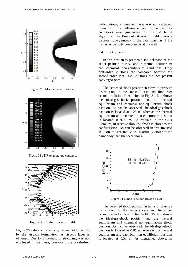
Figure 31 : Mach number contours.
Figure 32 : T/R temperature contours.
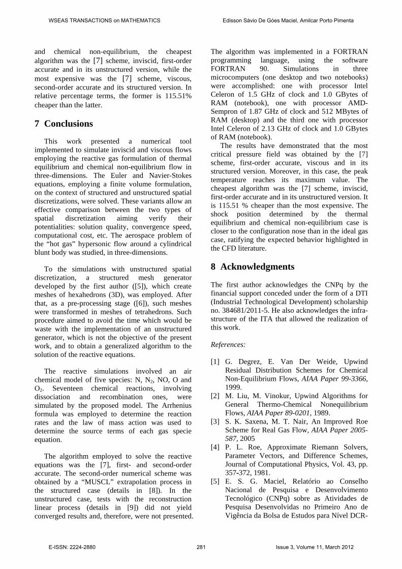
Figure 33 : Velocity vector field.
Figure 33 exhibits the velocity vector field obtained by the viscous formulation. A viscous layer is obtained. Due to a meaningful stretching was not employed in the mesh, preserving the tetrahedron
deformations, a boundary layer was not captured. Even so, the adherence and impermeability conditions were guaranteed by the calculation algorithm. The flow-velocity-vector field presents discrete non-symmetry in the determination of the Cartesian velocity components at the wall.
6.4 Shock position
In this section is presented the behavior of the shock position in ideal and in thermal equilibrium and chemical non-equilibrium conditions. Only first-order solutions are compared because the second-order ideal gas solutions did not present converged ones.
The detached shock position in terms of pressure distribution, in the inviscid case and first-order accurate solution, is exhibited in Fig. 34. It is shown the ideal-gas-shock position and the thermal equilibrium and chemical non-equilibrium shock position. As can be observed, the ideal-gas-shock position is located at 1.25 m, whereas the thermal equilibrium and chemical non-equilibrium position is located at 0.95 m. As referred in the CFD literature, in reactive flow the shock is closer to the configuration. As can be observed in this inviscid solution, the reactive shock is actually closer to the blunt body than the ideal shock.
Figure 34 : Shock position (inviscid case).
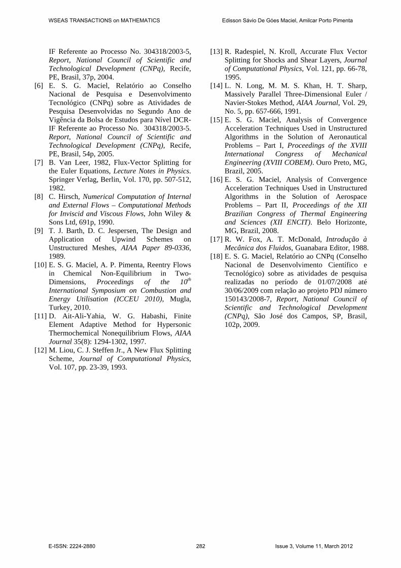
The detached shock position in terms of pressure
distribution, in the viscous case and first-order accurate solution, is exhibited in Fig. 35. It is shown the ideal-gas-shock position and the thermal equilibrium and chemical non-equilibrium shock position. As can be observed, the ideal-gas-shock position is located at 0.65 m, whereas the thermal equilibrium and chemical non-equilibrium position is located at 0.50 m. As mentioned above, in
WSEAS TRANSACTIONS on MATHEMATICS Edisson Sávio De Góes Maciel, Amilcar Porto Pimenta
E-ISSN: 2224-2880 279 Issue 3, Volume 11, March 2012
reactive flow the shock is closer to the configuration. As can be observed in this viscous solution, the reactive shock is actually closer to the blunt body than the ideal shock.
Figure 35 : Shock position (viscous case).
6.5 Computational performance of the studied algorithm
Table 3 presents the computational data of the reactive simulations performed with the [7] scheme to the problem of the cylindrical blunt body in three-dimensions. In this table are exhibited the studied case, the maximum number of CFL employed in the simulation, the number of iterations to convergence and the number of orders of reduction in the magnitude of the maximum residual in relation to its initial value to reach convergence. As can be observed, only in one case the convergence was assumed with three (3) orders of reduction in the value of the maximum residual: solution of the [7] second-order accurate, structured, inviscid, three-dimensional and in thermal equilibrium and chemical non-equilibrium. The maximum numbers of CFL presented the following distribution: 0.5 in two (2) cases (33.33%) and 0.1 in four (4) cases (66,67%). The maximum number of iterations to convergence did not overtake 6,800 iterations, in all studied cases. However, the time waste in the simulations was much raised, taking until weeks to convergence (four orders of reduction in the maximum residual). This can be verified in the computational costs presented in Tab. 4.
It is important to emphasize that all three-dimensional viscous simulations were considered as being laminar, without the introduction of a turbulence model, although high Reynolds numbers were employed in the simulations.
Table 3 : Computational data of the reactive simulations of the blunt body 3D.
Studied Case
CFL
Iterations Orders of Reduction
of the Residual
1st/S(1)/I(2) 0.5 291 4
1st/S/V(3) 0.5 1,445 4
2nd/S/I 0.1 6,100 3
2nd/S/V 0.1 6,703 4
1st/U(4)/I 0.1 2,003 4
1st/U/ V 0.1 3,854 4
(1)S = Structured; (2)I = Inviscid; (3)V = Viscous; (4)U = Unstructured.
Table 4 : Computational costs of the [7] scheme in the reactive cases.
Studied Case Computational Cost(1)
1st/Inviscid/Structured 0.0008824
1st/Viscous/Structured 0.0014364
2nd/Inviscid/Structured 0.0010906
2nd/Viscous/Structured 0.0016439
1st/Inviscid/Unstructured 0.0007628
1st/Viscous/Unstructured 0.0010994
(1) Measured in seconds/per iteration/per computational cell. Table 4 presents the computational costs of the [7] scheme in the three-dimensional reactive formulation to the structured and unstructured, first- and second-order cases. This cost is evaluated in seconds/per iteration/per computational cell. They were calculated employing a notebook with 2.13 GHz of clock and 1.0 GBytes of RAM, in the Windows Vista Starter environment. In the three-dimensional case, considering thermal equilibrium
WSEAS TRANSACTIONS on MATHEMATICS Edisson Sávio De Góes Maciel, Amilcar Porto Pimenta
E-ISSN: 2224-2880 280 Issue 3, Volume 11, March 2012
and chemical non-equilibrium, the cheapest algorithm was the [7] scheme, inviscid, first-order accurate and in its unstructured version, while the most expensive was the [7] scheme, viscous, second-order accurate and its structured version. In relative percentage terms, the former is 115.51% cheaper than the latter. 7 Conclusions
This work presented a numerical tool implemented to simulate inviscid and viscous flows employing the reactive gas formulation of thermal equilibrium and chemical non-equilibrium flow in three-dimensions. The Euler and Navier-Stokes equations, employing a finite volume formulation, on the context of structured and unstructured spatial discretizations, were solved. These variants allow an effective comparison between the two types of spatial discretization aiming verify their potentialities: solution quality, convergence speed, computational cost, etc. The aerospace problem of the “hot gas” hypersonic flow around a cylindrical blunt body was studied, in three-dimensions.
To the simulations with unstructured spatial discretization, a structured mesh generator developed by the first author ([5]), which create meshes of hexahedrons (3D), was employed. After that, as a pre-processing stage ([6]), such meshes were transformed in meshes of tetrahedrons. Such procedure aimed to avoid the time which would be waste with the implementation of an unstructured generator, which is not the objective of the present work, and to obtain a generalized algorithm to the solution of the reactive equations.
The reactive simulations involved an air chemical model of five species: N, N2, NO, O and O2. Seventeen chemical reactions, involving dissociation and recombination ones, were simulated by the proposed model. The Arrhenius formula was employed to determine the reaction rates and the law of mass action was used to determine the source terms of each gas specie equation.
The algorithm employed to solve the reactive equations was the [7], first- and second-order accurate. The second-order numerical scheme was obtained by a “MUSCL” extrapolation process in the structured case (details in [8]). In the unstructured case, tests with the reconstruction linear process (details in [9]) did not yield converged results and, therefore, were not presented.
The algorithm was implemented in a FORTRAN programming language, using the software FORTRAN 90. Simulations in three microcomputers (one desktop and two notebooks) were accomplished: one with processor Intel Celeron of 1.5 GHz of clock and 1.0 GBytes of RAM (notebook), one with processor AMD-Sempron of 1.87 GHz of clock and 512 MBytes of RAM (desktop) and the third one with processor Intel Celeron of 2.13 GHz of clock and 1.0 GBytes of RAM (notebook). The results have demonstrated that the most critical pressure field was obtained by the [7] scheme, first-order accurate, viscous and in its structured version. Moreover, in this case, the peak temperature reaches its maximum value. The cheapest algorithm was the [7] scheme, inviscid, first-order accurate and in its unstructured version. It is 115.51 % cheaper than the most expensive. The shock position determined by the thermal equilibrium and chemical non-equilibrium case is closer to the configuration nose than in the ideal gas case, ratifying the expected behavior highlighted in the CFD literature. 8 Acknowledgments The first author acknowledges the CNPq by the financial support conceded under the form of a DTI (Industrial Technological Development) scholarship no. 384681/2011-5. He also acknowledges the infra-structure of the ITA that allowed the realization of this work. References: [1] G. Degrez, E. Van Der Weide, Upwind
Residual Distribution Schemes for Chemical Non-Equilibrium Flows, AIAA Paper 99-3366, 1999.
[2] M. Liu, M. Vinokur, Upwind Algorithms for General Thermo-Chemical Nonequilibrium Flows, AIAA Paper 89-0201, 1989.
[3] S. K. Saxena, M. T. Nair, An Improved Roe Scheme for Real Gas Flow, AIAA Paper 2005-587, 2005
[4] P. L. Roe, Approximate Riemann Solvers, Parameter Vectors, and Difference Schemes, Journal of Computational Physics, Vol. 43, pp. 357-372, 1981.
[5] E. S. G. Maciel, Relatório ao Conselho Nacional de Pesquisa e Desenvolvimento Tecnológico (CNPq) sobre as Atividades de Pesquisa Desenvolvidas no Primeiro Ano de Vigência da Bolsa de Estudos para Nível DCR-
WSEAS TRANSACTIONS on MATHEMATICS Edisson Sávio De Góes Maciel, Amilcar Porto Pimenta
E-ISSN: 2224-2880 281 Issue 3, Volume 11, March 2012
IF Referente ao Processo No. 304318/2003-5, Report, National Council of Scientific and Technological Development (CNPq), Recife, PE, Brasil, 37p, 2004.
[6] E. S. G. Maciel, Relatório ao Conselho Nacional de Pesquisa e Desenvolvimento Tecnológico (CNPq) sobre as Atividades de Pesquisa Desenvolvidas no Segundo Ano de Vigência da Bolsa de Estudos para Nível DCR-IF Referente ao Processo No. 304318/2003-5. Report, National Council of Scientific and Technological Development (CNPq), Recife, PE, Brasil, 54p, 2005.
[7] B. Van Leer, 1982, Flux-Vector Splitting for the Euler Equations, Lecture Notes in Physics. Springer Verlag, Berlin, Vol. 170, pp. 507-512, 1982.
[8] C. Hirsch, Numerical Computation of Internal and External Flows – Computational Methods for Inviscid and Viscous Flows, John Wiley & Sons Ltd, 691p, 1990.
[9] T. J. Barth, D. C. Jespersen, The Design and Application of Upwind Schemes on Unstructured Meshes, AIAA Paper 89-0336, 1989.
[10] E. S. G. Maciel, A. P. Pimenta, Reentry Flows in Chemical Non-Equilibrium in Two-Dimensions, Proceedings of the 10th International Symposium on Combustion and Energy Utilisation (ICCEU 2010), Mugla, Turkey, 2010.
[11] D. Ait-Ali-Yahia, W. G. Habashi, Finite Element Adaptive Method for Hypersonic Thermochemical Nonequilibrium Flows, AIAA Journal 35(8): 1294-1302, 1997.
[12] M. Liou, C. J. Steffen Jr., A New Flux Splitting Scheme, Journal of Computational Physics, Vol. 107, pp. 23-39, 1993.
[13] R. Radespiel, N. Kroll, Accurate Flux Vector Splitting for Shocks and Shear Layers, Journal of Computational Physics, Vol. 121, pp. 66-78, 1995.
[14] L. N. Long, M. M. S. Khan, H. T. Sharp, Massively Parallel Three-Dimensional Euler / Navier-Stokes Method, AIAA Journal, Vol. 29, No. 5, pp. 657-666, 1991.
[15] E. S. G. Maciel, Analysis of Convergence Acceleration Techniques Used in Unstructured Algorithms in the Solution of Aeronautical Problems – Part I, Proceedings of the XVIII International Congress of Mechanical Engineering (XVIII COBEM). Ouro Preto, MG, Brazil, 2005.
[16] E. S. G. Maciel, Analysis of Convergence Acceleration Techniques Used in Unstructured Algorithms in the Solution of Aerospace Problems – Part II, Proceedings of the XII Brazilian Congress of Thermal Engineering and Sciences (XII ENCIT). Belo Horizonte, MG, Brazil, 2008.
[17] R. W. Fox, A. T. McDonald, Introdução à Mecânica dos Fluidos, Guanabara Editor, 1988.
[18] E. S. G. Maciel, Relatório ao CNPq (Conselho Nacional de Desenvolvimento Científico e Tecnológico) sobre as atividades de pesquisa realizadas no período de 01/07/2008 até 30/06/2009 com relação ao projeto PDJ número 150143/2008-7, Report, National Council of Scientific and Technological Development (CNPq), São José dos Campos, SP, Brasil, 102p, 2009.
WSEAS TRANSACTIONS on MATHEMATICS Edisson Sávio De Góes Maciel, Amilcar Porto Pimenta
E-ISSN: 2224-2880 282 Issue 3, Volume 11, March 2012